Durham E-Theses

Forced response prediction for industrial gas turbine

blades

Mo�att, Stuart

How to cite:

Mo�att, Stuart (2006) Forced response prediction for industrial gas turbine blades, Durham theses, DurhamUniversity. Available at Durham E-Theses Online: http://etheses.dur.ac.uk/2692/

Use policy

The full-text may be used and/or reproduced, and given to third parties in any format or medium, without prior permission orcharge, for personal research or study, educational, or not-for-pro�t purposes provided that:

• a full bibliographic reference is made to the original source

• a link is made to the metadata record in Durham E-Theses

• the full-text is not changed in any way

The full-text must not be sold in any format or medium without the formal permission of the copyright holders.

Please consult the full Durham E-Theses policy for further details.

Academic Support O�ce, Durham University, University O�ce, Old Elvet, Durham DH1 3HPe-mail: e-theses.admin@dur.ac.uk Tel: +44 0191 334 6107

http://etheses.dur.ac.uk

Forced Response Prediction for Industrial Gas Thrbine Blades

Stuart Moffatt

The copyright of this thesis rests with the author or ths university to which It was submitted. No quotation from It, or

Information derived from It may ba published without tha prior written consent of the author or university, and any Information derived from It should ba acknowladged.

A Thesis presented for the degree of

Doctor of Philosophy

School of Engineering

University of Durham

Durham, UK

November 2006

1 2 DEC 2006

Forced Response Prediction for Industrial Gas Turbine Blades

Stuart Moffatt

Abstract

A highly efficient aeromechanical forced response system is developed for pre­

dicting resonant forced vibration of turbomachinery blades with the capabilities of

fully 3-D non-linear unsteady aerodynamics, 3-D finite element modal analysis and

blade root friction modelling.

The complete analysis is performed in the frequency domain using the non­

linear harmonic method, giving reliable predictions in a fast turnaround time. A

robust CFD-FE mesh interface has been produced to cope with differences in mesh

geometries, and high mode shape gradients. A new energy method is presented,

offering an alternative to the modal equation, providing forced response solutions

using arbitrary mode shape scales. The system is demonstrated with detailed a

study of the NASA Rotor 67 aero engine fan rotor. Validation of the forced response

system is carried out by comparing predicted resonant responses with test data for

a 3-stage transonic Siemens industrial compressor.

Two fully-coupled forced response methods were developed to simultaneously

solve the flow and structural equations within the fluid solver. A novel closed-loop

resonance tracking scheme was implemented to overcome the resonant frequency

shift in the coupled solutions caused by an added mass effect. An investigation

into flow-structure coupling effects shows that the decoupled method can accurately

predict resonant vibration with a single solution at the blade natural frequency.

Blade root-slot friction damping is predicted using a modal frequency-domain ap­

proach by applying linearised contact properties to a finite element model, deriving

cont~ct pr()R~rties_ frpm a!l adya~ced ~~l!!i-an~yt~~aJ ~l~ro~iP_rno<ieL An_~§_et!s_-_~----- _____ ,

ment of Coulomb and microslip approaches shows that only the microslip model is

suitable for predicting root friction damping.

Declaration

The work in this thesis is based on research carried out in the Thermo-fluid Dynamics

Group, School of Engineering, University of Durham, Durham, UK. No part of this

thesis has been submitted elsewhere for any other degree or qualification and it all

my own work unless referenced to the contrary in the text.

Copyright © 2006 by Stuart Moffatt.

"The copyright of this thesis rests with the author. No quotation from it should be

published in any format, including electronic and the internet, without the author's

prior written consent. All information derived from this thesis must be acknowledged

accordingly".

lll

Acknowledgements

I would like to thank Prof. Li He for his continual support during the course of

this project and for sharing his extensive knowledge. His guidance and contagious

enthusiasm for the subject have been greatly appreciated.

The non-linear harmonic method has been developed at Durham University by

Prof. Li He, Dr. Wei Ning, Dr. Tie Chen and Dr. Parthasarathy Vasanthakumar

under sponsorship from Alstom UK.

I would also like to thank Dr. Haidong Li, Prof. Grant Steven and Dr. Jon

Trevelyan from the School of Engineering, Durham University, for their advice and

technical support.

This work has been done in close cooperation with Siemens, Lincoln. Many

thanks to Mr. Roger Wells, Dr. Wei Ning and Dr. Yansheng Li for their help and

support.

This research was sponsored by the European Union Framework V R&D project

"Development of Innovative Techniques for Compressor Aeromechanical Design (D IT­

CAD)", contract number ENK5-CT-2000-00086.

This document has been produced in ~'lEX-using a template created by M. Imran.

Many thanks to my brother lain for the crash course and the (extended) loan of the

manuals.

lV

Contents

Abstract

Declaration

Acknowledgements

1 Introduction

1.1 Motivation . .............

1.2 Background to the Physical System

1.2.1 Tur bomachinery Configurations

1.2.2 Aeroelastic Phenomena . .

1.2.3 Vibration Characteristics .

1.2.4 Unsteady Flow in Turbomachinery

1.2.5 Friction Damping

1.3 Research Objectives .

1.4 Overview of Thesis

1.5 Figures .....

2 Literature Review

2.1 Introduction ..

2.2 Computational methods for unsteady turbomachinery flows .

2.2.1 Governing flow equations .

2.2.2 Spatial discretisation . . .

2.2.3 Numerical integration techniques

2.3 Advances in unsteady aerodynamic methods

v

ii

iii

iv

1

1

3

3

4

9

12

14

16

18

20

23

23

24

24

25

25

26

Contents vi

20301 Time-marching methods 26

20302 Linearised methods 0 0 0 28

20303 Non-linear harmonic method 0 30

204 Structural Modelling ...... 31

2.401 Finite Element Analysis 32

2.402 Reduced Order Modelling 33

20403 FEA in Turbomachinery 35

205 Aeroelastic Modelling 0 0 0 0 0 0 37

20501 Decoupled Aeroelastic Methods 38

20502 Fully Coupled Aeroelastic Methods 42

206 Blade Root Friction Modelling 0 45

20601 Macroslip Models 45

20602 Microslip Models 47

20603 Application of Friction Models in Turbomachinery 0 48

207 Current State-of-Art •••••••• 0 • 0 •••••••••• 50

3 Computational Models and Methods 52

301 Non-linear Harmonic Method 52

301.1 Description •••• 0 • 52

301.2 Time-Averaged Equations 55

301.3 Harmonic Perturbation Equations 0 58

301.4 Boundary Equations 60

301.5 Solution Method 0 0 61

301.6 The TF3D Flow Solver 0 62

302 Structural Modelling 0 ••••• 64

30201 Finite Element Modelling 64

30202 Modal Reduction Method 65

303 Friction Damping Modelling 70

30301 Macroslip Models 70

30302 Microslip Model 0 74

30303 Implementation of Friction Models 77

3.4 Figures 0 0 0 0 0 0 0 0 0 0 0 0 0 0 0 0 0 0 0 0 80

Contents vii

4 Decoupled Forced Response System 89

401 Overview of Methodology 89

402 FE-CFD Mesh Interface 93

40201 Problem Description 93

40202 Metholology 0 0 0 0 0 94

40203 Mathematical Formulation 95

403 Modal Equation Method 99

4.4 Energy Method 0 101

405 Figures 0 0 0 0 0 0 105

5 Verification of the Decoupled System 108

501 Introduction 0 0 0 0 0 0 0 0 0 0 0 0 108

502 NASA Rotor 67 Transonic Fan 0 0 109

50201 Case Description 0 109

50202 Results 0 0 0 0 0 0 0 111

503 Siemens Three-Stage Transonic Compressor 0 114

50301 Case Description 0 114

50302 Results 0 . 117

5.4 Conclusions 0 0 0 119

5.401 NASA Rotor 67 'I\oansonic Fan 0 119

50402 Siemens Three-Stage Transonic Compressor 0 120

505 Figures 0 0 0 0 0 0 0 0 . 0 0 0 0 0 0 0 0 0 0 . ..... 0 122

6 Fully-Coupled Forced Response Methods 130

601 Introduction 0 0 0 0 0 0 0 0 0 0 130

602 Frequency Domain Method 0 0 131

603 Hybrid Frequency-Time Domain Method 0 133

604 Comparison with Decoupled Method 0 134

605 Resonance Tracking 0 0 0 0 136

606 Convergence Behaviour 0 0 138

607 Summary 0 139

608 Figures. 0 0 141

Contents viii

7 Fluid-Structure Coupling Effects 144

7.1 Introduction .... 144

7.2 Added Mass Effect 145

7.3 Modified Decoupled Method 146

7.3.1 Formulation . . . . . 146

7.3.2 Comparison of Coupling Methodologies . 147

7.3.3 Impact of Frequency Shift .... 148

7.4 Decoupled Prediction of Frequency Shift 149

7.5 Coupled Prediction of Frequency Shift 150

7.6 Sensitivity to Frequency Shift 152

7.7 Summary 155

7.8 Figures .. . 156

8 Friction Damping Analysis 161

8.1 Introduction ........ 161

8.1.1 Conventional FE approach 162

8.1.2 Overview of Adaptive Constraint Method . 163

8.2 Methodology .................... 164

8.2.1 Integration with decoupled forced response system . 164

8.2.2 Finite Element representation of friction contact . . 165

8.2.3 Adaptive Constraint Method . 166

8.2.4 Friction damping calculation . 168

8.3 Implementation . . . . . 168

8.3.1 Case description . 168

8.3.2 Calculation of contact stiffness . 169

8.4 Results .................. 171

8.4.1 Implied friction damping from forced response analysis 171

8.4.2 Coulomb friction results . 172

8.4.3 Microslip friction analysis . 177

8.5 Conclusions . 179

8.6 Figures ... . 181

Contents

9 Conclusions and Recommendations

9.1

9.2

Conclusions .. . .

9.1.1 Decoupled forced response system

9.1.2 Verification Cases . . ..

9.1.3 Fully-coupled forced response systems .

9.1.4 Fluid-structure coupling effects

9.1.5 Friction Modelling .. . .

Recommendations for Future Research

9.2.1 Forced response system .

9.2.2 Root Friction Modelling

Bibliography

ix

189

189

189

190

191

. 192

. 192

. 194

. 194

. 195

198

List of Figures

1.1

1.2

1.3

1.4

1.5

3.1

3.2

3.3

Collar's triangle of aeroelastic forces . . . . . . . .

Campbell diagram for a typical turbojet fan rotor

Interaction of aerodynamic excitation forces, aerodynamic damping

forces and mechanical damping forces with blade vibration

Compressor flutter map

Local stress concentrations at asperity junctions

Brick representation of Rigid Coulomb friction model

Rigid Coulomb friction force for increasing displacement

Rigid Coulomb friction force for sinusoidal displacement

20

21

21

22

22

80

80

81

3.4 Rigid Coulomb hysteresis curve . . . . . . . . . . . . . . 81

3.5 Variation of Rigid Coulomb friction work and damping ratio with

displacement amplitude. . . . . . . . . . . . . . . . . . 82

3.6 Brush representation of Elastic Coulomb friction model 82

3. 7 Elastic Coulomb friction force for increasing displacement . 83

3.8 Elastic Coulomb hysteresis curves for various amplitudes of displace-

ment .................................... 84

3.9 Variation of Elastic Coulomb friction work and damping ratio with

displacement amplitude . . . . . . . . . . . .

3.10 Microslip friction force during initial loading

3.11 Microslip friction hysteresis curve .

3.12 Microslip friction work at slip limit

3.13 Graphical representation of microslip and sliding work

3.14 Friction work predicted by the microslip model . . . . .

X

85

85

86

86

86

87

List of Figures xi

3.15 Variation in microslip damping ratio with displacement amplitude 87

3.16 Calculation of tangential stiffness using various positions on microslip

force curve . . . . . . . . . . . . . . . . . . . . . . . . . . . . . . . . . 88

4.1

4.2

4.3

Decoupled forced response system

Possible interpolation planes for a rectangular FE element face

2D interpolation at projection onto FE mesh surface

4.4 Calculation of orthogonal projection point ..... .

4.5 Transformation of interpolation points into local 2D geometrical axis

system ................... .

4.6 Equilibrium of forcing and damping work .

4. 7 Response phase for maximum forcing work

5.1 NASA Rotor 67 fan rotor geometry with contour plot of 2-node inlet

distortion . . . . . . . . . . .

105

105

105

106

106

106

107

122

5.2 Mode shape axial components 122

5.3 Comparison of natural frequencies with results of Marshall, 1996 123

5.4 Comparison of original and interpolated modeshape (axial component) 123

5.5 CFD mesh section and steady solution plotted at Ya span) 124

5.6 Inlet axial velocity and density distortion ..

5. 7 Inlet total pressure perturbation of solution

125

126

5.8 Mode 3, imaginary component of axial force and work in axial direction126

5.9 Cross section of Siemens 3-stage transonic compressor .

5.10 Strain gauge location on Rotor 2 blade

5.11 FE mesh of compressor blade . . . . .

5.12 Campbell diagram around 32E.O. crossing point with modes 8, 9 and

10 .......................... .

5.13 Axial modeshape components of modes 8,9 and 10 .

5.14 Comparison of original and interpolated modeshape for mode 9 axial

component .......................... .

5.15 Comparison of predicted and measured performance maps

6.1 Frequency-domain fully coupled system . . . . . . . . . . .

127

127

127

128

128

129

129

141

List of Figures xii

6.2 Hybrid fully coupled system 141

6.3 Coupled and decoupled solutions around resonant peaks for Mode 7 142

6.4 Resonance tracking using parabolic curve fitting . . . . 142

6.5 Convergence in frequency of resonance tracking scheme 143

7.1 Argand diagrams of modal amplitude of vibration-induced complex

modal damping force ......... .

7.2 Frequency response curves for Mode 7.

156

157

7.3 Frequency response curves for coupled and decoupled calculations 158

7.4 Argand diagrams of forces at solutions around resonance for Mode 3 . 159

7.5 Variation of combined excitation and damping aerodynamic force

with excitation frequency . . . . . 160

7.6 Sensitivity of coupled solutions at natural frequencies to fluid-structure

coupling effect ............................... 160

8.1 Application of friction calculation into decoupled forced response system 181

8.2 Friction contact nodes on surfaces of root flanks . . . . . . . . . . . 182

8.3 Spring representation of 3-D contact stiffness at each contact node . 182

8.4 Adaptive Constraint Method of FE friction modelling 183

8.5 Derivation of tangential stiffness from microslip curve 183

8.6 Nodal pressures after each static solution, showing convergence of

static contact analysis . . . . . . . . . . . . . . . 184

8. 7 Blade modal frequencies using Coulomb approach 184

8.8 Comparison of mode shapes for various methods of root constraint . 185

8.9 Tangential contact displacements at modal forced response solutions . 185

8.10 Mode 8 tangential contact displacements normalised to elastic limit . 186

8.11 Variation of damping ratio with response amplitude for mode 8, show-

ing individual node stick-slip transition points ............. 186

8.12 Comparison of microslip calculation with original calculation of Olof-

sson, 1995 ................................. 187

8.13 Variation of predicted microslip friction damping with position of

effective stiffness calculation for Mode 8 187

List of Figures xiii

8.14 Variation of predicted damping with response amplitude for Mode 8 . 188

List of Tables

5.1 Natural frequencies and modeshapes ..

5.2 Target inlet conditions and solution modal force

5.3 Aerodynamic damping . . . ..... .

5.4 Forced response solutions using modal method

5.5 Forced response solutions using energy method .

5.6 Natural frequencies . . . . . . . . . .

5.7 Aerodynamic and mechanical damping ratios.

5.8 Forced response solutions . . . . . . . . . .

6.1 Resonant conditions

111

112

113

114

114

117

118

119

135

6.2 Decoupled and coupled response predictions at blade natural frequency136

7.1 Comparison of decoupled and coupled resonant peaks ......... 148

7.2 Frequency shift due to viscous and inertial damping force components 151

8.1 Rigid and Elastic Coulomb friction damping predictions . . . . . . . . 173

8.2 Variation of predicted Elastic Coulomb friction damping with contact

stiffness . . . . . . . . . . . . . . . . . . . . . . . . . . . . . . . . . . 175

8.3 Variation of predicted Elastic Coulomb friction damping with normal

contact stiffness . . . . . . . . . . . . . . . . . . . . . . . . . . . . . . 175

8.4 Variation of predicted Elastic Coulomb friction damping with friction

coefficient . . . . . . . . . . . . . . . . . . . . . . . . . .

8.5 Rigid and Elastic Coulomb friction damping predictions .

XIV

176

177

Chapter 1

Introduction

1.1 Motivation

It is becoming widely accepted that forced response analysis must be integrated into

the design phase of all modern turbomachinery blades in aero-engine, industrial and

marine applications. Fluid flow through turbomachinery is inherently unsteady,

where strong periodic flow disturbances can cause high levels of blade vibration

for certain unavoidable resonant conditions. Flow-induced vibration has long been

recognised as the primary source of High Cycle Fatigue (HCF) blade failure a

problem regularly experienced throughout the gas turbine industry. The scale of the

problem is demonstrated by Kielb [1], who highlights that fluid-structure interaction

problems continuously arise during the development of each new machine, with every

jet engine development program experiencing 2.5 serious HCF problems on average.

Fransson [2] mentions that problems which are not discovered during development

are responsible for over 25% of all engine distress cases, accounting for almost 30%

of total development costs. Putting these costs into perspective, Wisler [3] states

that total development costs for an aero-engine can exceed $1 billion, with the

development of an aero-derivative engine costing up to $400 million. Additionally,

Kielb [4] indicates that HCF-related development and field usage costs incurred by

the US military could exceed $2 billion over the 20 years leading up to 2020.

The driving force to eliminate vibration problems is high for all turbomachinery

applications. Aero-engines are subject to stringent weight and size limitations and

1

1.1. Motivation 2

operate at a wide range of operating conditions, making them highly susceptible

to HCF problems - particularly for military jet engines. The process of achieving

airworthiness certification requires very vigorous testing, ensuring that most HCF

problems are uncovered during the development stage before potential failures can

arise in service. However, catastrophic engine failure with loss of life is not unknown

in civil and defence aerospace. Industrial and marine turbomachinery is subject

to less stringent safety regulations and weight and size limitations, allowing more

conservative designs to be adopted. These machines generally operate within a

less-demanding operating range, with some exceptions such as industrial pumps,

which can operate at off-design conditions for long periods of time. However, no

turbomachines are immune to blade vibration problems and the expense of a plant

shut-down can be very high, creating losses of up to £1 million per day in the case

of the shut down of an electrical power generation plant. Development budgets of

industrial turbomachines are normally much smaller than those of aero-engines, and

the expense of remedial redesign action following the discovery of a blade vibration

problem during testing can significantly increase the total development cost of a new

machine.

The occurrence of HCF problems is expected to increase in the future with cur­

rent trends in modern blade designs. In search of improved efficiency and reduced

engine size and weight, commercial pressures are demanding higher blade loading

and closer axial spacing, making modern blades more prone to high vibration levels.

Conventional design methodologies based on empirical design rules can not confi­

dently predict vibration levels and the assessment of aeromechanical performance is

achieved through rigorous engine testing. Analytical prediction methods are gener­

ally too costly for routine design use and are currently limited to the larger aero­

engine manufacturers. With increasing demands on aeromechanical performance

and without an early predictive capability, manufacturers run the risk of moving

towards a passive 'repair philosophy', using an iterative method of eliminating HCF

problems in new projects by redesigning blades based on engine test results. In or­

der to reduce lead times and development costs of new projects using modern blade

designs, there is a great need for a fast and reliable design tool for the prediction of

1.2. Background to the Physical System 3

flow-induced vibration levels. Such capabilities will allow blade designers to assess

vibration performance early in the design stage and eliminate potential HCF failures

before the first test is performed.

The work presented in this thesis involves the development and assessment

of aeromechanical forced response analysis methodologies based on finite element

analysis and computational fluid dynamics for the calculation of resonant blade

vibration levels. The methodologies are intended for routine design use with the

capability of accurately assessing resonant stress levels and predicting blade fatigue

life with minimal computational costs.

1.2 Background to the Physical System

1.2.1 Turbomachinery Configurations

A turbomachine is a rotating device for the purpose of either extracting energy

from a continuously flowing working fluid (turbine) or applying energy to the fluid

(compressor). Energy transfer in a turbine or compressor is made by respectively

decreasing or increasing the pressure of the fluid by the dynamic action of mov­

ing blades. The common elements of most turbomachines are a) a rotor, containing

blades, buckets or an impellor to decelerate or accelerate the flow; b) a shaft to trans­

fer mechanical power to or from the rotor; c) a casing to direct the fluid around rotor;

and d) stator blades in the form of inlet guide vanes or downstream blades to control

flow swirl around the annulus. Thrbomachines are categorised by the orientation of

the flow path: axial flow machines employ flow wholly or partially parallel to the

axis of the rotor; radial or centrifugal machines involve a flow path mainly normal to

the axis of rotation; and mixed flow machines contain significant amounts of radial

and axial flow components. Flow can be compressible or incompressible and is not

always enclosed within a casing, for example in the case of some fans, wind turbines

and tidal turbines.

Gas turbines are a common configuration of turbomachinery, which combine a

compressor and a turbine with the addition of heat to the fluid (normally air) in

order to generate shaft power or thrust. Incoming air is compressed and fed into a

1.2. Background to the Physical System 4

combustion chamber, where fuel is injected and burned. The resulting combustion

gases pass through a turbine to drive the compressor and the remaining high en­

ergy exhaust gases are used to provide useful power in the form of thrust or shaft

power from a secondary power turbine. Axial turbomachines are most commonly

used in aero-engine, industrial and marine gas turbine applications, mainly due to

the higher efficiency over their radial counterparts. Axial machines have relatively

thin blades and high aerodynamic loads and are more prone to aeroelastic prob­

lems than radial machines, which have fairly sturdy impellors. Axial turbomachines

usually comprise of several stages in order to achieve the necessary pressure ratios,

which can be up to around 20 stages for compressors and 5 stages for turbines, with

each stage comprising of one stator and one rotor bladerow. Whilst the analytical

methodologies described in this thesis can theoretically be applied to most turbo­

machinery configurations, the work contained herein focuses on air-breathing axial

gas turbines.

1.2.2 Aeroelastic Phenomena

Aeroelasticity is concerned with the static or dynamic interaction between the de­

formation of an elastic body and behaviour of a surrounding fluid. The study of

aeroelasticity is best described by Collar's triangle of forces (Figure 1.1), showing

the various levels of interaction between the fluid and structure. The interaction

of elastic and inertial forces is involved purely with mechanical vibration without

the influence of the surrounding fluid. The interaction between aerodynamic forces

and the inertia of a structure represents a rigid body subject to a fluid flow and is

typical of the type of problem encountered in aircraft stability and control appli­

cations. The interaction of fluid forces with the elastic deformation of a structure

neglects structural acceleration and is considered to be a static problem. Static

aeroelasticity is experienced by turbomachinery blades, where the steady-state fluid

loads of the mean flow result in the static deformation of the blades, varying the

aerofoil geometry. Combined with the effects of centrifugal and temperature load­

ing, the static deformation is known as blade untwist and small variations in blade

shape can have a significant impact on machine performance. The analysis of sta-

1.2. Background to the Physical System 5

tic blade deformation is very important in turbomachinery design, where the blade

must be manufactured to a certain profile, accounting for untwist to ensure that

the blade conforms to the correct geometry under normal operating conditions. Dy­

namic aeroelasticity provides the focus of the work within this thesis and relates to

flow-induced vibration problems, combining the effects of aerodynamic, inertial and

elastic forces. Dynamic aeroelastic analysis in turbomachinery poses a challenging

problem due to the complex interaction between high-speed fluid flow and the dy­

namic response of the blade structure. Whilst many forms of dynamic aeroelastic

behaviour exist throughout a range of engineering sectors, two of the most important

dynamic aeroelastic phenomena in turbomachinery applications are forced response

and flutter. This thesis primarily deals with the analysis of forced response, but as

discussed later, the methodologies can also be applied to flutter prediction.

Forced Response

Aeroelastic forced vibration is caused by periodic flow disturbances passing through

the blade passages, resulting in an unsteady pressure field acting on the blade sur­

faces. The aerodynamic excitation forces are primarily due to circumferential varia­

tions in the flow, normally caused by blades passing through the wakes of upstream

blades, potential interaction from upstream or downstream blades, non-uniform inlet

flow or from fluctuations in the back pressure. Resonant vibration occurs when the

frequency of the incoming flow disturbances matches a blade mode natural frequency,

which can lead to excessive blade stress amplitudes and eventual HCF failure. The

frequency of the flow disturbances in such synchronous excitation is normally pro­

portional to the speed of the rotor, denoted by the engine order (EO), giving the

integer number of disturbances experienced during one complete rotor revolution.

For example, a bladerow consisting of 32 blades will impart 32 EO wake disturbance

on the downstream bladerow, where the downstream rotor will experience an exci­

tation frequency equal to 32 times the frequency of rotation. The inlet distortion of

an aero fan subject to a cross wind will result in a 1 EO excitation at the frequency

of rotation.

An important tool for visualising when the flow disturbances cause resonant

1.2. Background to the Physical System 6

vibration is the Campbell diagram shown in Figure 1.2. This example maps the

frequencies and engine speeds of a large aero fan, showing where resonance is en­

countered from the individual engine orders. Such resonant conditions are named

crossing points, indicating where the frequency of a given EO coincides with a blade

natural frequency. It can be seen that the modal frequencies increase with engine

speed, which is due to centrifugal stiffening of the blade. Centrifugal stiffening oc­

curs when the blade is deformed out the plane of rotation or in the circumferential

direction. For a rotating beam, where the centre of gravity ( CG) of each section is

radially aligned, the radial centrifugal load will be reacted by a purely radial shear.

However, when the blade is deformed and the sections are deflected away from the

radial alignment, the blade shear reaction to the centrifugal load will provide a com­

ponent acting to re-align the section CG 's. This restoring force provides a stiffening

effect, thus increasing the frequencies of vibratory modes with engine speed.

The Campbell diagram can either be obtained analytically from a finite element

analysis (FEA) or experimentally in a rotating engine test using strain gauges placed

on the blades. In blade design, the Campbell diagram is used to place natural fre­

quencies either above the maximum engine speed or below the normal operating

range with the aim of avoiding continuous resonant excitation during operation.

However, crossing points at speeds below the operating range are always encoun­

tered during the start-up and shut down of each operational cycle, resulting in

resonant vibration contributing to HCF. Since resonance in turbomachines can not

be avoided, the vibration levels at all encountered crossing points must be evaluated

to determine the risk of fatigue failure during the service life of the machine.

Aeroelastic forced response prediction poses a challenging problem due to the

complex interaction between the fluid flow and blade structure. As illustrated in

Figure 1.3, blade vibration is caused by incoming flow disturbances creating a pe­

riodic pressure distribution over the blade surface. Consequently, the vibration of

the blade within the surrounding fluid induces a local unsteady pressure field in

the fluid around the blade surfaces. In forced response cases, the motion of the

blade through the vibration-induced pressure field results in energy dissipation to

the fluid, creating an aerodynamic damping effect. Combined with any mechanical

1.2. Background to the Physical System 7

damping present in the system, the total damping forces limit the amplitude of vi­

bration. Due to the high level of computation required by unsteady computational

fluid dynamic flow solvers, routine forced vibration analysis remains prohibitively

expensive for most manufacturers. Instead, designers rely on empirical design rules

and full-scale engine tests to evaluate vibration performance.

Designers have a number of options to reduce resonant vibration levels in the

eventuality that a particular crossing point creates a HCF risk. This can be done

either by moving the synchronous vibration frequency, reducing the aerodynamic

forcing function or incorporating friction dampers into the blading. Varying the

frequency of the crossing point can be done by either modifying the blade natural

frequency or by varying the blade count to change the forcing EO. A shift in natural

frequency can be achieved by varying the blade shape, changing parameters such

as thickness versus span, aspect ratio, taper, solidity and radius ratio. A drastic

method of increasing frequencies is the addition of a tip or part-span shroud to

stiffen the blades, usually with a secondary friction damping effect. Moving syn­

chronous frequencies outside the operating range is not always possible, particularly

for aero-engines, which operate within a wide range of speeds and conditions. An

additional point of interest regarding geometry change is that the resulting variation

in modeshape may have a significant effect on both the sensitivity of the mode to a

particular forcing function and the aerodynamic damping of that mode. This is due

to the positioning of the force distribution in relation to areas of high motion of the

modeshape.

The strength of the aerodynamic forcing function is strongly influenced by the

axial spacing between adjacent bladerows and the strength of upstream wakes can

generally be reduced by increasing the axial spacing. However, this action contra­

dicts the aims of modern designs which aim to minimise spacing to reduce engine

weight.

Flutter

Unlike forced response where blade excitation is provided by incoming flow distur­

bances, flutter is a self-excited phenomenon and is not caused by incoming external

1.2. Background to the Physical System 8

disturbances. Flutter occurs, when small levels of blade vibration are amplified

by the vibration-induced pressures giving rise to further blade excitation. Flutter

analysis can be considered in a similar manner to aerodynamic damping in forced

response problems, where the blade motion through the local induced pressure field

results in an energy transfer between the fluid and structure. The fundamental dif­

ference is that flutter causes the addition of energy to the blade instead of energy

dissipation. Flutter can therefore be considered as negative aerodynamic damp­

ing. As the self-exciting aerodynamic forces increase with blade motion, flutter can

quickly lead to escalating vibration levels causing fatigue failure within a short space

of time.

In flutter analysis, blade designers are interested in the flutter stability of the

system, determined by the direction of energy transfer between the blade and the

fluid. The system is stable when the vibration-induced pressures result in energy

dissipation (positive aerodynamic damping) and a decay of vibration amplitude.

Flutter instability occurs with energy application to the blade from the fluid, indi­

cated by a negative damping value. It can be argued that a system is stable with

small flutter forces, providing that sufficient mechanical damping is present to bal­

ance the destabilising fluid work. Under this condition, equilibrium will be achieved

and the blade will vibrate with a finite amplitude.

Flutter is predominantly seen in fans, front compressor blades and low pressure

turbine blades, and usually occurs above a critical flow velocity or when a high in­

cidence angle causes large flow separation. Since the 1940's when flutter was first

encountered in turbomachinery, the most important design parameters safeguard­

ing against flutter have been the reduced frequency and the incidence angle. The

reduced frequency is a non-dimensional parameter relating flow velocity with vibra­

tion frequency by comparing the period of one vibratory cycle with the time taken

for a fluid particle to travel a representative distance (i.e. chord length). The angle

of incidence is concerned with the degree of fluid loading on the blade, where flow

separation occurs at high values. In practice, the reduced frequency and the inci­

dence angle can only be used as a rough guide to indicate flutter stability since many

other critical factors often come into play, for example modeshape, nodal diameter

1.2. Background to the Physical System 9

pattern, and operating conditions such as pressure ratio and flow.

Flutter in turbomachinery applications is categorised into different areas, each

showing different characteristics and physical reasoning. The most important flutter

regions in a compressor are indicated on the performance map shown in Figure 1.4.

This figure also briefly introduces the main physical mechanisms behind stall, su­

personic and choke flutter. The details of various flutter are mechanisms beyond the

scope of this thesis and more in-depth descriptions are provided by Marshall [5] and

Fransson [6]. Ideally, flutter boundaries are placed at locations on the compressor

map that can not be reached during normal operation, a technique commonly called

"stall protection". Most modern engines have a relatively large stall margin, leav­

ing a sufficient margin to account for engine-to-engine variations, altitude effects,

transient operation and engine deterioration.

1.2.3 Vibration Characteristics

In turbomachinery applications, the vibration characteristics of a structure are

largely independent of the aerodynamic loads and are generally determined from

the mass and stiffness properties of the blade, together with any mechanical damp­

ing. This simplification is primarily due to the high density of blades compared

to the surrounding fluid, represented by the mass ratio. The mass ratio is defined

as the ratio of the mass per unit span of the structure divided by the mass per

unit span of a cylinder circumscribing the leading and training edges. Unlike the

aeroelastic analysis of aerofoils of lower density such as aircraft wings and helicopter

blades, forced response and flutter of turbomachinery blades usually involves the vi­

bration of a single mode, with very little mode interaction and a minimal variation

in modeshapes and natural frequencies by aerodynamic loading.

U nshrouded blades

Unshrouded blades, with their slender aerofoils, exhibit similar vibration charac­

teristics to beams and plates, particularly for low-order modes. Beam-type modes

give rise to flapwise, edgewise and torsional modes, but without chordwise bending.

The blade root can influence aerofoil modeshapes, particularly the constraints at

1.2. Background to the Physical System 10

the root / disk interface which effectively determine the stiffness of the lower part

of the blade. Unshrouded blades without under-platform dampers require a rigid

disk to avoid mechanical inter-blade coupling between blades, with coupling consid­

ered to be only provided by aerodynamic loading. The mechanically independent

nature of such blades greatly eases vibration analysis, usually allowing aeroelastic

calculations to be performed using a single blade analysis without the influence of

structural nonlinearities or disk dynamics.

Disc flexibility

The flexibility of the disk itself can have a significant effect on the overall char­

acteristics of the blades. A relatively rigid disk, such as used in a fan assembly,

will provide little influence on the individual blades, which will tend to vibrate in

their individual mode shapes. However, a flexible bladed disk assembly will include

the characteristics of the individual blades and the disk itself. Disk vibration is

characterised by nodal diameter modes, usually consisting of double modes. These

modes arise from the circular symmetry, where two consecutive modes possess the

same natural frequency with different orientations of modeshape. These modes oc­

cur in axial, radial and tangential directions. Disk vibration is characterised by

groups of nodal diameters, where each group is associated with a nodal circle. As

the mode number and natural frequency increase, the number of nodal circles in­

creases. Without the effect of additional friction dampers, the strong mechanical

coupling between the flexible disk and the blades effectively combines the assembly

into one structure, combining the natural frequencies of the blades and disk. For a

disk-dominated mode, the individual blade will vibrate in a mode with a significant

degree of general plane motion.

Shrouded blades

Shrouded blades offer greater rigidity with the mechanical coupling of adjacent

blades, resulting in significant disk vibration characteristics. The interlocking shrouds

provide a significant degree of friction damping and can be optimised for the de­

sired damping performance. However, the non-linear damping behaviour of friction

1.2. Background to the Physical System 11

damping creates difficulty in the aeroelastic analysis of shrouded blades.

The structural analysis of blade static and dynamic vibrational behaviour is gen­

erally finite element based. Cantilevered blades with rigid disks are often modelled

individually, neglecting disk dynamics and assuming that all blades are identical.

Analysis of flexible disk and shrouded assemblies take advantage of the cyclic sym­

metry, allowing the structure to be modelled as a segment with cyclic symmetric

boundary conditions and reducing computational effort. Other approaches model

the entire bladed disk and can include the effects of structural non-linearities and

variation in the properties of individual blades, but at the expense of high compu­

tational effort. It has also been known to use multi-stage models to capture the

mechanically coupling between stages.

Mistuning

A structural characteristic that can have a significant impact on the aeroelastic per­

formance of blades is mistuning. Blade mistuning arises when the cyclic symmetry

is broken by small geometric and structural variations in individual blades, resulting

from manufacturing processes or wear in service, causing a significant variation in

the aeroelastic performance of a system. Flutter stability has been reported to be

improved with blade mistuning, backed up by experimental and numerical evidence.

However, mistuning generally has a detrimental effect on forced vibration behav­

iour with the effect of amplifying the vibration levels of certain blades. Whereas a

tuned bladed disk assembly will show a single nodal diameter modeshape at a single

frequency, a mistuned assembly can simultaneously contain components of several

nodal diameters with slight variations in blade modeshapes and natural frequencies.

Therefore, the frequency response curve of a mistuned assembly will show a number

of resonant peaks around a particular crossing point, increasing the chance of being

excited by another excitation order. Hence, amplification in forced response can be

caused by secondary resonance from a disturbance of another excitation orders or

due to the variation in blade modeshape causing higher sensitivity to aerodynamic

forces. Forced vibration amplitudes of mistuned blades can be 100% higher than

vibration levels predicted for tuned blades (Ewins [7]). This so-called stress ampli-

1.2. Background to the Physical System 12

fication effect is caused by highly-localised bladed disc modeshapes amplifying the

responses of a small number of blades. The sensitivity of bladed disks to mistuning

has been found to be dependant on a number of parameters, including the amount

of interblade coupling present in the system and the densities in natural frequencies

of adjacent mistuned blades.

1.2.4 Unsteady Flow in Turbomachinery

Fluid passing through turbomachinery experiences strong time-dependant distur­

bances due to the complex nature of high-speed flow and the relative motion of

adjacent bladerows. Flow through a blade passage is subject to potential and

convective disturbances propagating from upstream sources, potential fields from

downstream bladerows and local vibration-induced pressures from the motion of the

blades themselves.

Bladerow Interaction

Bladerow interaction between relatively moving bladerows occurs due to the prop­

agation of wakes from upstream blades and the potential interaction between adja­

cent rows. Due to the high numbers of blades found in turbomachinery bladerows,

bladerow interaction normally involves high-frequency excitation of the higher-order

modes. In the case of a compressor wake, the wake produced by a blade is primarily

a reduction in the flow velocity. Therefore, a downstream blade passing through the

wake experiences a sharp perturbation in flow velocity due to the deficit in wake

velocity. In the case of a turbine blade wake, the velocity deficit in the wake is seen

by the passing blade primarily as a perturbation in the flow velocity but without

a significant change in the flow angle. In the past, wakes were determined by ex­

perimental measurements, yielding actual wake data or empirical correlations, but

modern methods often rely on steady CFD calculations.

Unlike blade wakes, potential disturbances have the capability to propagate up­

stream and interfere with convective disturbances and potential reflections. Poten­

tial interaction involves the propagation of a potential field created by an aerofoil,

which can travel both upstream and downstream in axially subsonic flow. Bladerow

1.2. Background to the Physical System 13

interaction can also involve the upstream propagation of shock disturbances, which

can cause strong shock excitation of upstream blades. In a transonic stage, a shock

can become detached from the blade passages, resulting in a leading edge shock that

can propagate upstream to reach the neighbouring bladerow. This type of shock ex­

citation has been known to create problems with the guide vanes of military fans. In

addition to leading-edge shock propagation, the trailing edge shocks of high-speed

vaneless HP turbine blades have been reported by Kielb [1], to reach the leading

edge of the LP turbine blades. The effects of potential and wake interaction are not

independent and the presence of the two disturbances can cause interference, either

amplifying or cancelling the effects of one-another.

Inlet Distortion

Another major source of blade excitation is inlet distortion, which describes dis­

turbances approaching the first stage due to circumferential non-uniformities in the

inlet flow. Inlet distortion is often encountered in aero fans and is seen in first

stages of compressors and high-pressure turbines. Unlike bladerow interaction, inlet

distortion usually provides a low EO excitation, affecting only the low-order modes

intersecting the first few engine orders.

Inlet distortion can be a significant problem for aero fans which often have non­

symmetric inlets and can operate with a non-zero angle of attack. Significantly high

angles of attack can result from high cross-winds and aircraft manoeuvres, including

take-off. Such conditions can cause a large region of flow separation at the inlet,

leading to substantial excitation of the fan. Inlet distortion is a particular problem

for military jet engines, which can have highly non-symmetric inlets and undertake

high agility manoeuvres. Land and marine-based compressors are subject to inlet

distortion from the non-uniformity of inlet ducts and the inclusion of struts in the

inlet. Gas turbine HP stages are subject to excitation from inlet temperature distor­

tions, provided by the hot streaks exiting the combustor cans. Due to the relatively

high number of combustor cans, temperature distortion provides an excitation EO

typically between 10 and 20. Inlet distortion can also be experienced by steam

turbines under partial flow conditions.

1.2. Background to the Physical System 14

1.2.5 Friction Damping

Background to Friction Modelling

Solid surfaces are inherently rough on a microscopic scale, causing the actual area of

contact between two solids to be much smaller than the apparent area of contact. It

is described by Bowden and Tabor [8] that "Putting two solids together is rather like

turning Switzerland upside down and standing it on Austria- the area of intimate

contact will be small". When two macroscopically fiat surfaces with microscopic

roughness are put in contact under a normal force, the load is transmitted through

a number of asperities of varying shape, size and height, as illustrated in Figure 1.5.

Local contact pressures are much greater than the average nominal pressure, giving

elastic or plastic deformation at the asperity junctions.

When the contact surfaces are subject to a relative tangential displacement, the

contact stress in each asperity is further increased until the elastic limit is reached

and the plastic flow of the asperity junction occurs. At this point, the asperity

is said to reach the transition from stick to slip. The result is a tangential force

opposing the motion, which increases with displacement until the yield stress is

reached, after which, the force remains constant as the asperity flows plastically.

The resulting effect is a tangential force opposing the direction of motion, which

increases with displacement up to a maximum value when the asperity reaches the

stick-slip transition. Since asperities vary in size, height and loading, each individual

asperity reaches plastic yield at different points on the loading cycle. Whereas

highly-loaded asperities can each yield with normal loading alone and slip with any

given tangential displacement, lightly-loaded asperities withstand a degree of elastic

deformation before slip. Under very small tangential displacements, lightly-loaded

asperities may not reach yield and will remain stuck. Friction forces are considered

to be the combined tangential forces of all individual asperity junctions acting over

the entire contact surface, where all asperities are subject to individual loading

conditions at various states in the stick-slip transition.

Due to the highly complex geometries of engineering surfaces at microscopic level

and the random nature of individual asperity properties, friction models simplify

1.2. Background to the Physical System 15

the underlying asperity mechanics to varying extents. Three friction models are

considered in this thesis: two macroslip friction models, which account only for

the net effects of two contacting surfaces; and a microslip friction approach, which

calculates the net effects based on the contributions of individual asperities.

Friction Damping in Turbomachinery

The sources of damping in turbomachinery blades are from vibration-induced fluid

pressures, friction at the blade root attachment, hysteretic material damping or any

additional friction dampers. Whilst damping data for root friction and hysteretic

damping is scarce, Kielb [9] provides a brief comparison for blades without addi­

tional friction dampers. He states that aerodynamic damping usually dominates for

the 1st bending, 1st torsion and 2nd torsion modes and that root friction normally

dominates for the 2nd and 3rd bending modes, whilst hysteretic damping is negli­

gible. Where additional friction dampers are used, Kielb states that well-designed

platform dampers can produce a critical damping ratio above 2%.

Friction damping occurs in regions of relative motion between contacting surfaces

in blade attachments or at the contact interface of friction dampers. The most

common type of damper is the platform damper, which usually takes the form of a

wedge-shaped piece of metal. Platform dampers can either rest against two adjacent

blades (blade-blade damper) or be placed between each individual blade and the

disk (blade-ground dampers). Blade-blade dampers utilise the relative movement

between adjacent blades, causing a sliding motion between the contact points of

the damper and each blade. The friction force is strongly dependant on the inter­

blade phase angle (IBPA) of the blade movement and causes a degree of mechanical

coupling between each blade. Blade-ground dampers are attached to the disk, with

frictional forces caused by the blade motion in relation to the disk without interaction

between neighbouring blades. Platform dampers are used on most high-pressure

turbine blades and some fan, compressor and low pressure turbine blades. Some

gas turbine manufacturers make it mandatory to include platform dampers on all

high-pressure turbine blades to allow for low-order blade excitation from flow non­

uniformities created with the ageing of the machines, such as partial vane burnout.

1.3. Research Objectives 16

Other methods of providing friction damping incorporate tip shrouds, part-span

shrouds or split-ring dampers. Shrouds normally have the primary intention of

increasing the natural frequencies of high aspect ratio blades, such as aero fan blades

and LP turbine stages. The nature of the interlocking shrouds can provide useful

levels of friction damping and damping performance is becoming an integral part of

shroud design. Split-ring dampers in the form of metal rings can be used between

blisk stages for the damping of the low nodal diameter nodes.

1. 3 Research 0 bjectives

The objective of the project is to develop effective methodologies to integrate the

non-linear harmonic aerodynamic method with structural dynamics for blade forced

response predictions. The intention of the research is to provide a complete aerome­

chanical analysis tool capable of providing routine resonant forced response calcula­

tions for turbomachinery blade designers under the commercial restraints of solution

times and computing resources. Various coupling strategies are to be implemented

for the purpose of evaluating the capabilities of decoupled and fully-coupled methods

to capture important flow-structure coupling effects. In addition, the effects of fric­

tion damping within 'fir tree'-type blade root attachments is to be investigated, with

the development of a friction analysis method and a study on the overall sensitivity

of the aeroelastic system to friction.

The non-linear harmonic method has been developed by the University of Durham,

providing an efficient frequency-domain unsteady flow solution, capable of dealing

with significant flow non-linearities. The method has been previously validated for

both rotor-stator interaction and oscillating blade cases. Further validation of the

fluid solver has been done in parallel with this project by members and industrial

partners of the University.

The basic strategy for the blade structural dynamics is to take a standard com­

mercial finite element (FE) package as the baseline analysis method to produce

detailed mode shapes and natural frequencies for all the blade vibration modes of

interest. The FE package used is Ansys 7.1, a standard code commonly used by

1.3. Research Objectives 17

turbomachinery designers. The modal reduction technique will be used to decouple

the structural equations, reducing the forced response calculation to a single degree­

of-freedom (DoF) for each mode of interest. The forced response calculation for each

mode of interest is performed in modal space based on the CFD mesh.

An FE-CFD mesh interface is to be developed for the interpolation of mode

shape data onto the CFD mesh. The interface must accurately interpolate mode­

shapes from an unstructured FE mesh to a structured CFD mesh and be capable of

dealing with a variety of element types and shapes. The interface must prove to be

sufficiently robust in order to deal with the complexities of industrial use, such as

high modeshape gradients with low density meshes and slight variations in geometry

between meshes.

The interaction between fluid and structure will be performed in the frequency

domain for compatibility with the flow solver. A separate analysis is conducted for

each mode of interest at the operating points given by the respective crossing points

of the Campbell diagram. Two distinct coupling philosophies are to be implemented:

• Decoupled approach. Fluid and structure are calculated separately, forming

an open-loop system with minimal interaction. Two separate executions of

the fluid calculations provide the aerodynamic excitation and damping terms,

which are subsequently used to solve the decoupled forced response equation.

• Fully-coupled approach. Fluid and structure are integrated simultaneously

within the CFD code, forming a closed loop system with tight coupling between

the aerodynamic forces and structural response.

The blade root friction damping analysis is to be carried out using an FE model

of the blade and the methodology must be compatible with the frequency-domain

aeroelastic calculations to provide friction damping predictions with minimal user

effort and computational time. The approach is to linearise the friction contact and

allow the highly-efficient modal reduction approach to be exploited. Both Elastic

Coulomb friction and microslip friction are to be considered and an evaluation of

the sensitivity of damping predictions to the fidelity of contact modelling will be

carried out.

1.4. Overview of Thesis 18

The NASA Rotor 67 transonic fan rotor will be used as the primary test case

during the development of the methodologies due to the relative simplicity of the

case and the availability of published data. This case will be used to demonstrate

the application of the forced response systems and provide a basis for further inves­

tigations into fluid-structure interaction.

Validation of the forced response system is carried out on the last stage rotor

of a Siemens three-stage industrial transonic compressor. Initial verification on the

accuracy of the forced vibration predictions will be checked against strain gauge data

obtained from full-scale rotating compressor tests, provided by Siemens. This case

is to be used for the analysis of root friction damping, where damping predictions

will be compared with damping measurements from test data.

1.4 Overview of Thesis

This thesis is divided into eight chapters, including this introductory chapter. The

literature review is given in Chapter 2, starting with a fairly comprehensive overview

of CFD developments and leading to an overview of structural modelling techniques

with an emphasis on FE analysis. A description of FE-CFD coupling methodolo­

gies then follows, and the chapter concludes after a review of friction modelling in

turbomachinery applications.

Chapter 3 introduces the computational models and methods employed, starting

with a summary of the non-linear harmonic method used in the fluid calculations,

followed by a overview of the finite element method and a detailed description of the

modal method further developed in this thesis. An overview of the current Coulomb

and microslip friction models is given with an explanation of how such models can

be implemented into the aeroelastic analysis.

Chapter 4 provides a detailed explanation of the decoupled forced response sys­

tem and the major components, in particular, the FE-CFD mesh interface, and the

modal reduction theory used in the aerodynamic forcing, damping and forced re­

sponse solution. Additionally, a new energy method of forced response solution is

presented. A demonstration and validation of the decoupled forced response system

1.4. Overview of Thesis 19

and system components is provided in Chapter 5, using case studies of the NASA

Rotor 67 transonic aero fan and a Siemens 3-stage transonic test compressor.

Two fully coupled forced response methods are presented in Chapter 6, based

on a frequency-domain and a hybrid frequency-time domain approach, leading to

an evaluation against the decoupled method, the implementation of a closed loop

resonance tracking scheme and an investigation into the convergence behaviour of

the coupled solution. Significant fluid-structure coupling effects were found in the

coupled solution due to a fluid added mass effect, which is further investigated in

Chapter 7, based on a variation of the decoupled method. An investigation into the

sources of resonant frequency shift in both decoupled and fully-coupled methods is

performed, leading to a study of sensitivity of a solution to frequency shift. The

chapter concludes with an evaluation of the use of decoupled and fully-coupled

methods for forced response prediction.

Chapter 8 describes a method for predicting blade root friction damping in the

frequency domain based on an advanced microslip friction model, to provide the

highest degree of compatibility with the aeroelastic forced response system. Im­

plementation of Coulomb and microslip models into ANSYS are described, and an

evaluation of the suitability of such friction models for predicting root friction damp­

ing is given. Initial validation of the friction damping predictions is given for the

Siemens test compressor.

The thesis concludes with Chapter 9, summarising the conclusions and providing

recommendations for future research.

1.5. Figures

1.5 Figures

Rigid Body Aerodynamics

Aeroelasticity

Mechanical Vibration

Figure 1.1: Collar's triangle of aeroelastic forces

20

1.5. Figures

~----------------------------------------,

300

¥ "-'200 ~ c u :::s 150 !" u..

100

--n _.2F --18

---0 ~~------------------------------------~

0 500 1 000 1500 2000 2500 3000 3500 4000 4500 5000

Rotor Speed (RPM)

Figure 1.2: Campbell diagram for a typical turbojet fan rotor

Unsteady q Blade ¢::)

Aero Flow Vibration Damping

Upstream disturbances fr Vibration-induced

• Inlet distortion Mechanical pressures

• Blade wakes Damping

• Material damping

• Friction

21

Figure 1.3: Interaction of aerodynamic excitation forces, aerodynamic damping

forces and mechanical damping forces with blade vibration

1.5. Figures

Mass Flow

1 Subsonic stall flutter

2 Transonic stall flutter

3 Choke flutter

4 Supersonic started flutter at low back pressure

5 Supersonic started flutter at high back pressure

Figure 1.4: Compressor flutter map

Elastic or plastic deformation at asperit junctions

Figure 1.5: Local stress concentrations at asperity junctions

22

Chapter 2

Literature Review

2.1 Introduction

Aeroelasticity in turbomachinery is a multidisciplinary subject based around struc­

tural mechanics and unsteady fluid dynamics, usually involving the integration of

finite element analysis (FEA) and advanced CFD methods. Due to the high com­

putational demands of unsteady CFD calculations, the development of aeroelastic

methods in recent years has generally progressed with advances in CFD. Much of

the research on CFD has been focused on reducing the computational demands of

the direct solution of the unsteady flow equations, which is normally prohibitively

expensive for multistage turbomachinery applications. Similarly, advances in FEA

have resulted in a number of techniques for reducing computational effort using var­

ious mathematical approaches and model techniques. For a particular application,

the choice of structural modeling technique and the strategy for flow-structure cou­

pling are largely dictated by the type of flow solver used, where methods of coupling

have been established for specific types of CFD analysis. Whilst friction modelling

has been used for many years in structural analysis, the use of friction models within

aeroelastic calculations is starting to emerge, driven by the need to optimise friction

damper design. Such friction models involve modelling contact surfaces at micro­

scopic level to varying degrees, which vary significantly from empirical relationships

based on experiment to advanced analytical calculations. Integration techniques be­

tween friction models and aeroelastic calculations are relatively immature and levels

23

2.2. Computational methods for unsteady turbomachinery flows 24

of integration are subject to large variation.

This chapter starts with a fairly comprehensive overview of developments in un­

steady CFD methods, which have had the strongest influence in the progress of

turbomachinery flutter and forced response calculations. An outline of significant

developments in structural modelling is given, with a particular emphasis on FE

analysis and the common approaches for reducing computational effort. An outline

of flow-structure coupling methodologies is given, describing the common config­

urations for integrating FEA with CFD. The chapter concludes with a review of

the development of various friction models and implementation into structural and

aeroelastic calculations.

2.2 Computational methods for unsteady turbo-

machinery flows

2.2.1 Governing flow equations

The governing system equations for a CFD model are obtained from the Conserva­

tion Laws of fluid flow through a discretised computational domain. These laws can

be condensed into a compact form to give the full system of Navier-Stokes equations,

providing the general description of fluid flow. The Reynolds-averaged Navier-Stokes

equations with turbulence modelling can predict viscous flow in great detail and can

include the mechanisms of aerodynamic losses and vortices. However, the high

accuracy of the Navier-Stokes equations is at the expense of high computational

demands. By making the assumption of inviscid, isentropic flow and neglecting the

viscous stress terms in the Navier-Stokes equations, a simplified system of equations

is derived - the Euler Equations, which are less computationally demanding. This

simplification provides an accurate description of a fluid with highly turbulent flow

with high Reynolds number, where the effects of boundary layers can be neglected.

Traditionally, the Navier-Stokes and Euler equations were used to perform the - --. ~ -~ -- -- - -

steady flow analysis, which forms the basis of turbomachinery blade design. How­

ever, unsteady flow analysis is a more complex problem due to the temporal variation

2.2. Computational methods for unsteady turbomachinery flows 25

in the flow field. Both the Navier-Stokes and Euler equations can be applied to un­

steady flow where the time-dependent variables are represented discretely either in

the time-domain or in the frequency-domain as Fourier coefficients.

2.2.2 Spatial discretisation

Spatial discretisation techniques currently used for CFD analysis largely fall into

two categories: finite difference and finite volume. The finite difference scheme

is the oldest method used to obtain solutions of differential equations and is the

simplest to apply. However, it is not commonly used in turbomachinery analysis,

instead being mainly used in external aerodynamics. The finite difference scheme

requires an orthogonal mesh with uniform spacing. For analysis of realistic cases, a

transformation from the physical mesh to a computational mesh is required. Trans­

formation is difficult for complex geometries, such as that of turbomachinery, but is

more straightforward for more common profiles, as used in external aerodynamics,

where transformation procedures and corresponding grids are used routinely.

The finite volume scheme, widely used in turbomachinery analysis, involves the

discretisation of the fluid domain as a continuum, divided into a finite number of

control volumes. The discretised equations are represented in integral form as fluxes

through the control volumes, satisfying the conservation laws. This approach allows

calculations to be performed in the physical domain and since no transformation

is required, the method can be used for complex 3D geometries of any mesh type.

Mesh types fall into one of two categories: structured finite difference meshes and

unstructured finite volume meshes.

2.2.3 Numerical integration techniques

Time-marching is commonly adopted for high speed compressible flow. The flow

equations are integrated in time and solved at each time step using either an explicit

or implicit time-marching scheme. The implicit scheme couples every point of the

domain simultaneously at each time step. Whilst the solution of a large number of

linear simultaneous equations may seem undesirable, this method is unconditionally

2.3. Advances in unsteady aerodynamic methods 26

stable and can be used for large time-steps. The simplest of these to implement is

the explicit scheme, where each point on the mesh is solved in turn at each time

step. The simplicity of this method therefore arises due to the lack of simultaneous

equations. However, the scheme is only stable for small time step length, requiring

large numbers of steps and longer computing times.

2.3 Advances in unsteady aerodynamic methods

Numerous schemes for the solution of the Euler or Navier-Stokes equations have been

developed for calculating steady flow through blade passages or unsteady flow due to

blade vibration and propagating aerodynamic disturbances from adjacent bladerows

or unsteady inlet conditions. Steady flow calculations currently provide the basis

for new turbomachinery designs. However, it is now realised that the calculation of

unsteady flow is becoming more important to ensure further improvements in aero­

dynamic performance and structural integrity. A great deal of progress has been

made in the use of numerical methods for the calculation of unsteady flows. U n­

steady CFD schemes can generally be divided into non-linear time-marching schemes

and time-linearised frequency-domain methods.

2.3.1 Time-marching methods

The most popular approach for solving the steady and unsteady non-linear flow

equations is the time-marching technique, where the equations are discretised on

a computational grid and marched until all transients have decayed to achieve ei­

ther a steady-state steady solution or a periodic unsteady solution. Computational

difficulties arise in time-marching solutions due to large size of system equations,

which can be up to the order of 106 . Additional difficulties arise due to the need

for a sufficiently small time-step to capture the important flow disturbances as well

as meeting the stability requirements for explicit schemes. Whilst non-linear time­

marching provides a powerful insight into complex flow phenomena, it is usually too

time-consuming for routine industrial use. Nevertheless, with increases in comput­

ing resources, many techniques have been made to maximize accuracy and reduce

2.3. Advances in unsteady aerodynamic methods 27

computational requirements.

The early explicit MacCormack scheme (MacCormack [10]) dominated practi­

cal CFD use until the early 1980's, solving the 2D Euler equations. Jameson [11]

developed the popular explicit central difference scheme, a method similar to that

of MacCormack which utilised the finite volume discretisation. Several 2D Euler

codes have since been developed, such as those used by Fransson and Pandolfi [12];

Gerolymos [13]; and He [14] for the calculation of flows around oscilating blades, and

by Giles [15] for bladerow interaction calculations. However, the use of 2D meth­

ods have been shown to be inadequate for aeroelastic applications (Namba [16];

Chi [17] and Hall & Lorence [18], where significant 3D effects have been found to

be present. The fully-3D calculation of the Euler equations have been reported by

Gerolymos [19], Hall and Lorence [18] and Marshall and Giles [20] for the use in

flutter and forced response calculations. Inviscid flow calculations are often used

in turbomachinery design but are not always suitable for aeroelastic calculations

for cases with significant viscous effects, such as flow separation, recirculation and

shock-boundary layer interaction can greatly affect blade response. Under these

circumstances, a viscous solution is required. The solution of the 3D Navier-Stokes

equations has been reported by He and Denton [21] for flow around vibrating blades

and Rai [22] and Chen et al. [23] for bladerow interaction problems.

The modelling of unsteady flow with temporal and circumferential periodic dis­

turbances has created computational difficulties as multi passage or whole annulus

solutions are often required. The implementation of phase-shifted boundary condi­

tions reduces computational effort by allowing a whole annulus to be represented by

a single passage. Erdos [24] was first to implement phase-shifted boundary condi­

tions for the 2D Euler equations by developing the direct store method, which was

used by Gerolymos [13] in 2D inviscid flutter calculations. The direct store method

requires vast computer storage and is prone to convergence issues. Rai [25] proposed

an alternative to periodic boundary conditions by modifying the blade numbers of

a rotor-stator turbine stage to allow a directly repeating boundary condition in a

small number of passages. The time-inclined method proposed by Giles [15] imple­

mented phase-shifted boundary conditions by transforming the flow equations into

2.3. Advances in unsteady aerodynamic methods 28

a computational time-domain, but is subject to limitations on the rotor-stator pitch

ratio and inter-blade phase angle (IBPA). The Fourier shape correction method of

He [26, 27] allows single passage domains to be used with phase-shifted boundary

conditions, overcoming problems with storage requirements. However, for complex

flow and multi-stage calculations, direct periodicity does not exist and multi-passage

or whole annulus domains must be used.

2.3.2 Linearised methods

Compared with the high level of computation associated with non-linear time­

accurate solutions, time-linearised methods provide a highly efficient means of un­

steady flow calculation. This frequency-domain approach eliminates the need for

high temporal resolution and allows a single passage calculation to be performed

without the difficulties in implementing phase-shifted boundary conditions, as seen

in time-accurate methods. In time-linearised methods, unsteady flow is decomposed

into steady and unsteady parts, where linear harmonic flow perturbations are super­

imposed onto a steady flow solution. Introducing a pseudo-time derivative into the

time-linearised Euler ro Navier-Stokes equations, the system can be solved using a

range of well-established time-marching schemes to give the steady-state harmonic

amplitudes. The harmonic perturbation equation is based on the nonlinear steady

solution and is solved in the frequency domain independently of the steady part to

yield the harmonic amplitude of the perturbation. The perturbation equation rep­

resents a single frequency and a more general solution can be obtained by combining

individual solutions at multiple frequencies. However, forced response analysis usu­

ally only requires a single flow harmonic at the blade natural frequency of interest,

based on the assumption that all frequencies outside the natural frequency have no

effect on the steady state vibration amplitude.

Classicallinearised methods, such as that of Whitehead [28] were based on tables

of flow data of unloaded flat plate cascades, where flow coefficients could be derived

for standard geometries for use in analytical flat plate theory. The introduction

of computers allowed semi-analytical formulations to be solved, normally with the

assumptions of inviscid, irrotational and incompressible flow. Developments of this

2.3. Advances in unsteady aerodynamic methods 29

type were applied to subsonic flow by Whitehead [29], transonic flow by Namba [30]

and supersonic flow by Verdon and McCune [31]. Whilst these methods could have

been useful in the aerodynamic design, they are not suitable for practical aero­

dynamic or aeromechanical analysis. These methods do produce accurate results

for the conditions in which they are intended and provide an invaluable bench­

mark for the validation of modern CFD solvers. An important development of the

method is the computer program LIN SUB by Whitehead [32], which can calculate

several important types of unsteady inviscid flow around a fiat plate cascade, such

as wake/rotor interaction, potential interaction and blade vibration.

The development of time-linearised potential flow methods, such as those of

Whitehead [33] and Verdon and Caspar [34], enabled the analysis of real aerofoils,

where the steady flow is based on the solution of the non-linear potential equations.

A later development of the potential method by Hall and Verdon [35] includes the

effects of incoming vertical and entropic disturbances to allow the calculation of

wake-rotor interaction. The need to capture transonic flow details with higher ac­

curacy led to the time--linearised Euler method of Ni [36]. This approach was later

developed by Hall and Crawley [37], who solved the linearised unsteady 2D Euler

equations using shock fitting giving accurate results, but this proved difficult for

complex three-dimensional shocks. Lindquist and Giles [38] showed that shock cap­

turing schemes could accurately model three-dimensional shocks with greater ease.

Linearised schemes have subsequently been developed into fully-3D methods by Hall

et al. [39] and Marshall and Giles [20].

The efficient linearised Euler methods were very successful but were limited to

flow conditions with insignificant viscous effects. Viscous effects can be significant

in aeroelastic problems which often occur at off-design conditions, for example at

part-speeds, where viscous flows become important. One of the first time--linearised

Navier-Stokes solvers was the 2D hybrid viscous-inviscid approach of Cizmas and

Hall [40]. Holmes et al. [41] were amongst the first to extend the linearised Navier­

Stokes to a fully-3D analysis, but using a turbulence model that limited the scheme

to flows with a thin attached boundary layer. Clark and Hall [42] produced a 2D

linearised Navier-Stokes solver using a turbulence model capable of dealing with

2.3. Advances in unsteady aerodynamic methods 30

large flow separations in stall flutter and Sbardalla and Imregun [43] reported a 3D

viscous linearised method capable of dealing with off-design conditions. Typically

being of two orders of magnitude faster than the equivalent time-domain solutions,

time-linearised methods offer a powerful unsteady flow prediction tool for blade

designers. However, the non-linear effects are neglected, which can reduce accuracy

for cases with features such as shock oscillation and flow separation.

2.3.3 Non-linear harmonic method

Until recently, CFD analysts were limited to the use of expensive non-linear time­

marching methods or efficient, but less accurate linearised methods. Whilst lin­

earised methods were developed as an efficient alternative to time-marching schemes,

they are limited to linear flow conditions. The non-linear harmonic method relieves

this limitation, exploiting the efficiency of the linearised frequency-domain methods,

whilst capturing some important non-linear effects of the time-accurate solutions.

Giles [44] devised a linearised Euler method that recognised changes in the non­

linear steady flow field due to the linear unsteadiness by introducing quadratic source

terms to the steady solution. He [45] adopted the idea of updating the steady so­

lution and proposed the non-linear harmonic method. Instead of using the steady

solution as a base, He included the deterministic stress terms, due to the unsteadi­

ness, to produce the time-averaged solution. Unsteady flow is modelled by superim­

posing the unsteady harmonic perturbations onto the time-averaged flow. The use

of pseudo-time-marching allows the use of well-established efficient algorithms to

be used. Non-linear interaction between the time-averaged and flow perturbations

is included by solving the perturbation equations together with the deterministic

stress terms to modify the time-averaged flow. Non-linearity between the individ­

ual perturbation harmonics can be included by simultaneously solving the harmonic

equations in a strongly coupled manner.

The non-linear capability is further improved by increasing the number of har­

monics of the perturbation equation to give a higher-order representation of the

flow unsteadiness. A method developed by Hallet al. [46] uses a harmonic balance

technique, representing the flow variables by a Fourier series in time with spatially

2.4. Structural Modelling 31

varying coefficients, in a similar fashion to the Fourier shape correction method of

He [26, 27]. The method can be applied to the Euler or Navier-Stokes equations

and is shown by Hall et al. to provide reasonable predictions for strongly nonlinear

flow. This approach has been adopted by Vasanthakumar [47] and implemented into

the non-linear harmonic method to provide a system where both the deterministic

stress terms of the time-averaged flow and cross-coupling terms of the individual

harmonics are solved simultaneously with flow perturbation equations.

The non-linear harmonic method has been extended to the three-dimensional

solution of the Navier-Stokes equations and used for the accurate prediction of flow

due to blade vibration (Vasanthakumar et al. [48]) and Stator-Rotor interaction

(Chen et al [49]). It has been shown to produce results with comparable accuracy to

three-dimensional viscous non-linear time-marching schemes, but with a consider­

able saving of processing time and storage requirements. Validation of the baseline

solver against semi-analytical solutions is given by Vasanthakumar et al. [48] for

inviscid flow through unloaded 2-D and 3-D vibrating flat plate cascades and by

Chen et al. [49] for wake blade interaction in a uniform steady flow past an un­

loaded flat blade cascade. Chen et al. also verify the non-linear capability of the

non-linear harmonic method for a single stage compressor by comparing the deter­

ministic stresses with those obtained from non-linear time marching in both 2-D

and 3-D. Verification on the use of the linear method for bladerow interaction in a

subsonic turbine stage and a transonic counter-rotating prop fan is provided by Ning

et al. [50], who showed qualitative and quantitative agreement with test data and

non-linear time-accurate solutions. The ability of the method to predict bladerow

interaction is further verified against test data for a transonic turbine stage by Ning

et al. [51].

2.4 Structural Modelling

Much of the earlier work on turbomachinery structural dynamics focussed purely

on predicting the natural frequencies of bladed disc assemblies for the intention of

designing the machines to operate outside resonant conditions. The early pioneer of

2.4. Structural Modelling 32

turbomachinery vibration was Campbell [52], who identified the characteristics of

vibrational modes of steam turbine bladed discs, and discovered the importance of

mistuning, resulting from blade-blade variations in material properties and geome­

tries. The first attempts at modelling the dynamic response of bladed discs involved

the analytical solutions of continuous models. Bishop and Johnson [53] used recep­

tance coupling substructure analysis, modelling the blades with Euler beam theory

and then coupling them to the disc by combining the frequency responses. Con­

tinuous models were also solved by energy conservation principles, using the well­

established Rayleigh-Ritz method. Whilst these methods have since been replaced

with discrete modelling, they are often used in the validation of numerical schemes.

2.4.1 Finite Element Analysis

The Finite Element (FE) method is a numerical technique for solving a range of phys­

ical problems, where the governing equations are represented by algebraic, differen­

tial or integral equations. Often being the first choice for detailed structural analy­

sis, finite element analysis (FEA) discretises the distribution of a variable through

a complex geometry by dividing the region into small elements of simple geome­

tries. The elements are interconnected mathematically at the nodes, ensuring that

the boundary of each element is compatible with its neighbour whilst satisfying the

global boundary conditions. The simple geometry of the elements allows the distri­

bution of the variable through the element to be defined by a simple shape function

- usually polynomial or trigonometric. The discretisation of the body allows the

governing equations for each element to be calculated and assembled into matrix

form to give the system equations. The manner in which the element equations are

constructed and the physical variables required in the analysis are dependent on

the nature of the physical problem, but always involves the specification of nodal

coordinates material properties and loading conditions. All physical problems are

broken down into a series of matrix equations, where the governing equations of the

system take a specific form for the type of problem to be solved.

Finite element analysis, therefore, breaks down a complex problem into a series

of coupled equations in matrix form, which are normally solved using general pur-

2.4. Structural Modelling 33

pose solvers. Due to fact that most structural properties are linear, most dynamic

structural calculations are performed in the frequency domain to save computa­

tional effort. Any non-linearities such as friction damping can be incorporated into

the forcing functions of the right-hand side of the dynamic equations. Frequency

domain solutions are usually solved using eigenvalue methods, but other approaches

include the harmonic balance method and the state-space method. Problems incor­

porating high non-linearity or complicated forcing functions can be solved using one

of the many time-integration schemes available in commercial solvers. Such time­

marching schemes are usually much more time-consuming than frequency-domain

approaches. The size of FE matrices can easily reach sizes of 106 square, providing

a large computational task and a number of methods can be adopted for reducing

the computational effort.

2.4.2 Reduced Order Modelling

Various techniques have been adopted in order to reduce computational costs of

FEA, particularly for dynamic analyses. There are numerous strategies for improv­

ing efficiency, and common techniques approach the problem by either conditioning

or reducing the element matrices.

Modal Reduction

Modal reduction provides a convenient method for solving the coupled dynamic

equations by expressing the displacements of the masses within a structure as a

linear combination of normal system modes. The dynamic response to a harmonic

disturbance of arbitrary frequency is considered to be a combination of the contri­

butions of all modes of the structure in the vicinity of the disturbance frequency.

Based on the results of a modal analysis, the response of each mode under consider­

ation is calculated individually, to yield the modal amplitudes. During this process,

the contribution of each individual mode to the disturbance is calculated separately

before being superimposed to give the total system response.

It has been previously discussed that the resonant response of a structure to a

harmonic disturbance at a particular natural frequency is characterised by the mode

2.4. Structural Modelling 34

shape, where the motion of every point on the structure vibrates harmonically and

in phase at the excitation frequency, and with a specific relative amplitude. The

motion of the structure is therefore 'locked' into that particular mode, where the

motion of the entire structure can be defined by a single representative amplitude.

Analogous to a single-DoF oscillator, the modal reduction technique calculates the

response of each mode in modal space, governed by a series of single DoF modal equa­

tions. The modal transformation therefore uncouples the large number of coupled

dynamic equations of the FE model to a series of uncoupled second-order differential

equations, which are easily solved.

Since modal reduction is a linear approach, it is suitable for systems where the

mass and stiffness matrices are constant. The major cost of modal methods is in

the calculation of the individual modes, so the method is better suited to cases that

can be modelled using a small number of modes.

Lumped Mass

The mass of a standard FE model is consistently defined throughout each element,

with the mass distribution defined by the element shape function. This results in a

non-diagonal mass matrix, which is difficult to include in the dynamic solution. A

common method for obtaining a diagonal mass matrix is to place discrete masses

at each node, resulting in a diagonal lumped mass matrix. The mass distribution is

discontinuous through the element and each discrete mass is calculated to preserve

the total element mass. The lumped mass method used by Ballhaus & Goorjian [141]

is the most computationally efficient and has been used for aeroelastic calculations

where reduced computational requirements take priority. In addition to the gain

in efficiency, it is also recognised that the lumped mass matrix results in higher

accuracy for the analysis of thin structures such as blade aerofoils.

Static Condensation

In many circumstances, some degrees of freedom do not significantly contribute to

the behaviour of the system and it is not necessary to solve the model using every

DoF. The process of static condensation simplifies the problem with the selection

2.4. Structural Modelling 35

of 'master' and 'slave' DoF to eliminate the unwanted DoF from the solution. For

example, the in-plane displacements of a thin aerofoil may be selected as slaves,

then condensed out of the system using the technique commonly known as Guyan

reduction (Guyan [55]). The resulting order of the mass and stiffness matrices are

reduced by the number of slave DoF.

2.4.3 FEA in Turbomachinery

Multistage turbomachines consist of several mechanically-coupled bladed disk as­

semblies, subject to various effects of disk dynamics, rotor dynamics, inter-stage

coupling and bearing effects. Without some sort of model simplification of such

large systems, the structural analysis alone would give rise to excessively large FE

models for aeromechanical analysis. Early structural analysis was concerned only

with predicting the natural frequencies of the blades or bladed disk assemblies to

allow blade designers to avoid resonant crossing points on the Campbell diagram.

More recent aeromechanical methods involve a similar approach including the cal­

culation of the blade modeshapes, which are usually prescribed onto the CFD mesh

based on the assumed modes method.

Tuned Systems

The simplest approach to finite element modelling is to model only one blade within

the bladerow, exploiting the cyclic symmetry of the geometry and neglecting the

mechanical coupling between blades through the disk structure. A single blade is

modelled either as a cantilevered aerofoil constrained at the hub, neglecting mechan­

ical coupling between blades or the disk. This method is appropriate for capturing

flow-structure coupling effects in most turbomachinery problems.

For cases with significant inter-blade mechanical coupling, such as for shrouded

bladed discs, it is more common to model the structure using cyclic symmetry,

reducing the whole bladed disk to a single sector model. Each sector consists of

one blade, a portion of disk and any shrouds, which is subject to complex boundary

conditions at the periodic boundaries of the sector-sector interfaces. In aeroelastic

calculations utilising multi-passage CFD solutions, the cyclic symmetry approach

2.4. Structural Modelling 36

allows the full assembly modal mass to be derived, which can not be done using

a single blade FE model. An additional consideration is that the modes change

smoothly between adjacent blades, instead of the step changes would occur between

blades if the sector modes were expanded from a single blade.

The tuned approach has been used in decoupled aeroelastic calculations of tuned

bladed disks by Chiang and Kielb [56], Manwaring and Kirkeng [57], Green and

Marshall [59], Filsinger et al. [60] and Tran et al. [61] and fully-coupled calculations

by Gerolymos [62], Marshall [5], Tran et al. [61].

Mistuned Systems

The assumption of cyclic symmetry allows highly detailed FE models of bladed disks

to be produced using a single blade sector, but this approach implies that all blades

are identical without the effects of mistuning. Mistuning results from blade-blade

variations in geometry and material properties caused by manufacturing tolerances

and in-service wear. The result typically has a detrimental effect in forced response

cases, where vibration is concentrated to a small number of blades, amplifying stress

levels beyond those of a tuned system in a phenomenon known as localisation. The

direct approach to mistuning would be to run several full whole-bladed-disk FE

models with randomly mistuned blades, but this would be too costly in terms of

terms of CPU time and storage space. Predicting the effects of mistuning requires

computationally efficient methods of performing free-vibration and forces response

calculations of full assembly models. Several methods have been developed to reduce

the size of large FE models of industrial bladed disk assemblies.

Early methods using lumped parameter models were reported by Ewins [63],

Griffin and Hoosac [64], Wei and Pierre [65]. Such models were used in the first inves­

tigations of mistuning, when the implications of mistuning were not well-understood

and the amplification effect was loosely described in terms of complex modes. The

mode localisation behaviour was realised by Wei and Pierre using a singe-DoF model

per blade sector based on modal reduction of the spring-mass system. By represent­

ing the system as an eigenvalue problem, Wei and Pierre also revealed that sensitivity

to mistuning increases with mode density.

2.5. Aeroelastic Modelling 37

The component mode synthesis method of Craig and Bampton [66] reduces the

number of DoF of the bladed disk, by considering each blade sector as a separate FE

model, represented by a summation of the sector eigenvalues and eigenvectors using

modal reduction. Based on the FE solution of a single blade sector, the modes and

frequencies of each individual sector component are mistuned, then assembled to

allow the complete mistuned assembly to be analysed. Variation between the prop­

erties of sectors is usually given randomly and a series of reduced-order solutions

can be analysed statistically. Craig-Bampton approaches have been implemented

by Irretier [67], Zheng and Wang [68] and Castanier et al. [69]. In a similar manner,

Yang and Griffin [70] combine the frequency response functions using receptance

techniques. A further development in the use of the component mode synthesis

method is by Bladh et al. [71] who investigates the effects of mechanical inter-stage

coupling between adjacent bladerows on the sensitivity to mistuning. Moyroud et

al. [72] provide a comparison of the Craig-Bamton method and a modal decompo­

sition of a full assembly against an unreduced full FE analysis of for tuned and

mistuned cases, including a shrouded transonic fan assembly. Monte-Carlo simula­

tions using statistical methods provide an alternative approach to the modelling of

mistuning, as described by Myhre et al. [73]. However, whilst various methods have

been developed to attempt to model mistuning, the mechanisms behind mistuning

and the implications on blade vibration are not yet fully understood and no reliable

prediction method is currently available.

2.5 Aeroelastic Modelling

Dynamic aeroelastic modelling techniques for forced vibration and flutter calcula­

tions involve the integration of unsteady aerodynamics with structural dynamics.

Various levels of fluid-structure coupling can be employed, depending on the cou­

pling strategy adopted. The type of coupling approach chosen for a particular

application is generally determined by the availibility of computing resources, the

type of fluid solver used and the need to include fluid or structural non-linearities.

At a fundamental level, aeroelastic methods are divided into decoupled and coupled

2.5. Aeroelastic Modelling 38

categories.

Decoupled approaches are based on an open-loop architecture, where the fluid

and structure are solved separately with uni-directional transfer of information on

a linear basis. Whilst decoupled approaches were originally developed for linearised

aerodynamic methods, the method allows a wide range of aerodynamic solutions

to be incorporated. The decoupled method is the most common choice for typical

turbomachinery cases due to its high computing efficiency.

Fully-coupled schemes are based on closed-loop architecture. The fluid and struc­

ture are normally integrated simultaneously in time, exchanging instantaneous forces

and displacements at each step in the solution. Modern fully-coupled schemes are

usually associated with non-linear time-accurate CFD solvers, which are capable

of intrinsically capturing flow and structural non-linearities. However, the com­

putational costs of time-accurate CFD codes are usually too high for routine use,

resulting in fully-coupled methods being limited mainly to research and diagnostic

applications.

2.5.1 Decoupled Aeroelastic Methods

Decoupled methods treat the fluid and structure in a linearised manner with a min­

imal degree of interaction between the two domains. The approach is based on

the assumptions of linear aerodynamic damping and that blade natural frequencies

and mode shapes are not affected by aerodynamic loading. These assumptions are

generally valid for turbomachinery blades, which are of high density and stiffness in

relation to the surrounding fluid and vibrate with low amplitudes. This unidirec­

tional approach allows the aerodynamic calculations to be performed independently

to the blade dynamics, offering considerable savings in computing requirements. It

is commonly accepted that mode shapes effectively remain unchanged for lightly

damped turbomachinery blades, and this assumption has been widely adopted i.e.

Kielb [9]; Marshall and Imregun [5]). Linear damping has been observed for tran­

sonic fan rotors by Li and He [74] and Schmitt et al. [75].

In a decoupled aeroelastic analysis, blade structural dynamics are firstly obtained

with a free vibration calculation to provide the blade modeshapes and natural fre-

2.5. Aeroelastic Modelling 39

quencies. The analysis is then done for a single mode at the corresponding natural

frequency. Traditionally, the decoupled method has been used for flutter prediction

and has been extended to forced response calculations in more recent years. Flutter

calculations are concerned with determining the aeroelastic stability of the system,

indicated by the direction of energy flow resulting from the blade vibrating in the

fluid. A decoupled flutter prediction therefore involves calculating the vibration­

induced pressures due to blade motion in the specified mode shape. In a forced

response analysis, the aerodynamic analysis involves the calculation of aerodynamic

damping for the given mode, in a similar manner to a flutter calculation; and the

calculation to the aerodynamic forcing terms, providing blade excitation from the

incoming flow disturbances.

Flutter

The flutter phenomenon has been experienced since the advent of the earliest air­

craft soon after the turn of the 20th century, leading to the first aeroelastic prediction

methods. Some of the first flutter calculations of isolated aerofoils were performed

by Theodorsen and Garrick [76], who modelled the bending and torsion of an aero­

foil section in incompressible potential flow; and by Goland [77], who applied a

known aerodynamic load to the differential equation solution of a uniform cantilever

beam. An important early development in turbomachinery aeroelastic analysis was

by Lane [78], who provided the general solution for a tuned cascade and showed that

a linear system of identical blades can be represented by a single equivalent blade,

where the vibration of all blades are assumed to occur with the same amplitude and

with a fixed interblade phase angle.

A significant advance in the prediction of flutter boundaries was the Energy

Method proposed by Carta [79], which calculates the net energy transfer between a

vibrating body and the flow-induced pressures of the surrounding fluid. Based on

the isolated flat plate theory of Theodorsen [80], Carta evaluated the logarithmic

decrement of a shrouded bladed disc as the ratio of work done by fluid pressures

to the average kinetic energy of the system. The energy method is based on the

assumption that the flutter occurs in a single natural mode of vibration, neglecting

2.5. Aeroelastic Modelling 40

the effect of mode modification by aerodynamic forces. The energy method was

further developed by Mikolajczak et al. [81], who generalised Carta's method to

include mechanical damping and drag force based on fiat plate cascade theories.

The assumed modes approach provides the basis of all decoupled aeroelastic

methods for flutter and forced response calculations. The eigensolution approach

provides a very flexible method of combining a variety of aerodynamic methods with

structural dynamics using an assumed mode approach, where the simplified struc­

tural representation in the frequency domain allows significant savings in solution

times. The aerodynamic forces can be obtained from almost any source, either di­

rectly frequency domain or transformed from the time-domain into the frequency

domain by means of Fourier analysis. The eigensolution method was introduced

into turbomachinery applications by Bendiksen and Friedmann [82] who combined

Theosdorsen's model with Lane's assumption to predict the effect of bending and

torsion on the flutter stability of a tuned cascade. Kaza and Kielb [83] developed

the method to predict mistuned cascade flutter, and Kielb and Ramsey [84] went

on to model supersonic fan flutter using fiat plate cascade theory.

The solution of the 2-D potential equations in decoupled flutter analysis has

been done by Verdon and Caspar [85], Whitehead [86] and Hall [87]. The solution

of the Euler equations has been done in 2-D by Takahara et al. [88], and Hall and

Crawley [37]; and in 3-D by Hall and Lorence [18]. The solution of the Navier-Stokes

equations in decoupled flutter calculations has been reported for 2D calculations by

Giles and Haimes [89]; and for 3D calculations by Siden [90], He and Denton [21],

Clark and Hall [92], and Chassaing and Gerolymos [93].

Forced Response

The main difference between a forced response analysis and a flutter analysis is the

inclusion of the incoming flow disturbances providing blade forced vibration and the

calculation of resulting blade response. Whereas a flutter analysis is concerned with

the direction of energy flow between a vibrating blade and the induced fluid forces,

a forced response analysis involves the calculation of: a) incoming flow disturbances;

b) aerodynamic damping; and c) blade modal response. The decoupled approach

2.5. Aeroelastic Modelling 41

allows the aerodynamic excitation and damping loads to be derived independently

from a wide range of sources, such as from flow measurements, empirical models or

CFD calculations.

Early forced response calculations of fiat plate cascades were based on the frozen

gust assumption of Whitehead [29], where a vortical inlet disturbance is assumed to

be convected downstream without being distorted by the flow field. An extension to

this approach by Goldstein and Atassi [94] introduced a degree of wake distortion for

an isolated aerofoil in incompressible flow. Aerodynamic damping calculations us­

ing similar fiat plate cascade theory were given for subsonic flow by Whitehead [28],

transonic flow by Namba [30], and supersonic flow by Verdon and McCune [31]. The

use of measured wake data to determine incoming flow disturbances is described by

Manwaring and Fleeter [95] who carried out extensive experimental studies of un­

steady loading of compressor blades under distortions, wakes and potential fields.

Examples of empirical modes include Mugridge and Morfey [96] and Raj and Lak­

shminarayana [97].

Modern decoupled forced response methods are based around CFD calculations,

usually solving the linearised 3-D Euler equations (Giles [44]; Hall et al. [39]). An

early example is by Chiang and Kielb [56], who produced a forced response system

combining both semi-empirical and analytical fluid calculations in order to minimise

computing costs of the CFD calculations. The incoming inlet flow disturbances

providing blade excitation were modelled using a semi-empirical rotor wake-vortex

model, measured data from the inlet distortion and a quasi-3D Euler solver for the

pressure disturbances. This work demonstrated both the flexibility of the decoupled

forced response method and the ability to efficiently predict vibration levels on a

routine basis.

The use of linearised CFD calculations of both aerodynamic damping and forcing

terms is described by Kielb [98], who presents a resonant forced vibration analysis of

an aeroengine fan rotor under inlet distortion subject to aerodynamic and structural

damping. Manwaring and Kirkeng [57] describe the forced response of a low pressure

turbine blade due to circumferential pressure distortion involving the 3-D solution

of the linearised Euler equations. Campobasso and Giles [99] describe an extension

2.5. Aeroelastic Modelling 42

of the decoupled method to the analysis of mistuned systems, where the decoupling

of aerodynamic loads allows a detailed investigation on mistuning effects.

The use of non-linear time-marching CFD schemes is less popular with the de­

coupled method and a flexible interfacing technique has been reported by Moyroud

et al. [100]. Additionally, Schmitt et al. [75] use a variation of the decoupled ap­

proach based on the the superposition of aerodynamic forces to evaluate the use of

both decoupled and fully-coupled forced response methodologies. Rather than the

traditional consideration of aerodynamic damping as an equivalent viscous damping

ratio, Schmitt et al. directly apply the vibration-induced pressures to the modal

equation.

The decoupled method is particularly suited for resonance tracking schemes,

where a number of forced response calculations are needed to capture large shifts

in resonant frequency due to friction dampers. Green and Marshall [59] present

a method of modelling a rotor acceleration of a high pressure turbine blade with

under-platform dampers. Aerodynamic forcing and damping terms obtained from

a linearised 3-D Euler solver are interpolated and scaled over the frequency range,

before being passed to a non-linear transient dynamics solver. In a similar manner,

Breard et al. [101], describe a decoupled frequency sweep with friction damping

using a 3-D viscous time-marching scheme, neglecting aerodynamic damping.

2.5.2 Fully Coupled Aeroelastic Methods

Whilst aeroelastic behaviour remains fairly linear under many operating conditions,

the need to model more complex flow-structure coupling effects with significant non­

linerities has lead to the development of fully coupled methods. With the rise in

popularity of time-marching CFD schemes in the 1980's, fluid-structure coupling

methodologies soon emerged that solved the fluid and structural equations simul­

taneously, usually in the time domain. In fully-coupled approaches, the level of

interaction between the fluid and structural domains can vary from partially in­

tegrated schemes to fully integrated schemes. Partially integrated schemes solve

the fluid and structural domains separately, exchanging information at each step

in the solution. Inter-grid interpolation is required at each step and one of several

2.5. Aeroelastic Modelling 43

interfacing schemes can be used to transfer data between the fluid and structural

meshes (i.e. Steger and Benek [104]; Rai [105]; and Moyroud [100]). Fully inte­

grated methods combine the fluid and structural equations into a single numerical

integration scheme, solving the entire system without the need to transfer informa­

tion between meshes at each step. Whilst fully-coupled methods involve a greater

degree of computation, they allow the inclusion of most nonlinear effects, with the

capability of providing less conservative flutter stability boundaries where limit cycle

behaviour is experienced. A second benefit of the fully-coupled method is that the

inter-blade phase angle providing the greatest instability automatically comes out

of the solution, rather than being an input requirement to the decoupled solution.

Flutter

The partially-integrated flutter method, developed by BaUhaus and Goorjian [141],

involves the simultaneous solution of the fluid and structure, each of which are

considered separately. Structural dynamics are usually based on the free-vibration

modal properties of the structure, which can be obtained numerically from a finite

element or analytical model, or from experiment. The modal representation greatly

reduces computational effort by reducing the structural equations to a small number

of orthogonal modal equations which can be integrated in time. Alternatively, a full

finite element model can be integrated in time in parallel with the CFD solver, where

the fluid pressure distribution at each time step is fed back to the FE package. A wide

variety of aerodynamic models can therefore be incorporated with little restriction

on the choice of fluid solver used.

Early investigations of stall flutter m linear cascades were done by Sisto et

al. [106] and Abdel-Rahim et al. [107] based on a 20 vortex and boundary layer

method for incompressible flow. Each 2D blade section was represented by a 2

DoF spring model, solving the bending and torsion equations of motion. Bakhle et

al. [108] utilised a similar rigid blade structural model, coupled with a 3D nonlinear

potential flow model. He [109] performed flutter and rotating stall calculations on

a cascade in two structural degrees of freedom using a 2D Navier-Stokes solver. A

number of more sophisticated methods based on 3D Euler and Navier-Stokes solvers,

2.5. Aeroelastic Modelling 44

integrated with FE models have been developed by Vahdati and Imregun [110], Mar­

shall [5], Chew et al. [111] and Hwang and Fang [112].

Fully integrated methods consider both the fluid and structure as a single con­

tinuum, where the fluid and structural equations are discretised such that they can

be integrated in time using a single numerical scheme. The method was pioneered

for flutter by Bendiksen [113], who integrated the Lagrangian-Eulerian formulation

of the aeroelastic equations in time using a 5-stage Runge-Kutta time-marching

scheme. The simultaneous solution of the flow and structural equations eliminates

any possible time lag in the coupling between the two domains, and is claimed to

predict energy transfer with greater accuracy than partially integrated schemes.

The disadvantage of fully coupled methods is the high computing costs associated

with integrating the fluid and structure. One method of reducing computational

demands is to implement a hybrid approach, such as the method of Gerolymos [19].

In this approach, the time-domain solution of the 3D Euler equations is coupled

with the frequency-domain modal solution of the structural dynamics. Based on a

free vibration modal analysis, the motion of a blade mode shape and a given inter­

blade phase angle is prescribed onto the CFD mesh and the aerodynamic solution

is marched for one period. After each period, the blade mode shape is recalculated

based on the aerodynamic coefficients and the cycle is repeated until convergence

of the blade mode in the frequency domain is achieved. This method improves the

computing efficiency over fully coupled methods whilst maintaining the ability to

model the nonlinear effect of aerodynamic forces on mode shape.

Forced Response

The development of fully coupled forced response methods has occurred only fairly

recently with advances in computing power. Providing the most realistic simula­

tion of fluid-structure coupling effects, fully coupled schemes normally involve the

time-accurate representation of the viscous compressible flow. Fully-coupled forced

response analyses usually involve the linear modal solution of the blade dynamics for

the purpose of reducing computation. Sayama et al. [114] solve the Favre-averaged

unsteady Navier-Stokes equations by means of non-linear time-marching, where the

2.6. Blade Root Friction Modelling 45

fluid mesh is deformed at each step according to the structural motion such that

changes in aerodynamic damping and flow unsteadiness are accommodated. Based

on a linear modal analysis, structural non-linearities, such as friction dampers are

included through an iterative modal solution. The application of the scheme for in­

let distortion and bladerow interaction cases for compressor fans and turbine stages

with the inclusion of friction damping are described by Vahdati et al. [115] and

Breard et al. [101]. In addition, a similar approach based on linear structural dy­

namics is applied to a counter-rotating prop fan by Schmitt et al. [75] for the purpose

of evaluating decoupled methodologies.

2.6 Blade Root Friction Modelling

Friction is defined as the tangential force opposing the relative motion of two sur­

faces in contact that are subject to a normal pressure. Frictional forces are often

very difficult to calculate accurately as they depend on many physical properties

of the surface topography, materials, loading conditions and the presence of any

contaminants. The evolution of friction models over the last century has yielded

a variety of approaches that can be placed into two categories: macroslip and mi­

croslip. Macroslip models offer the most simple approach, based on the classical

Coulomb friction theory and assuming rigid motion of a body over a contact sur­

face. Microslip models offer greater fidelity for conditions with small displacements

and high pressures, by incorporating the effects of local deformation of the contact

surfaces on a microscopic scale.

2.6.1 Macroslip Models

The most common understanding of friction is Coulomb friction, developed by

Amontons and Coulomb during the late 17th and 18th centuries, respectively. Coulomb

friction corresponds to dry, unlubricated surfaces, and states that the whole friction

surface is either stuck or sliding. The frictional force is determined by either a static

or dynamic coefficient of friction, relating to the ratio of the tangential frictional

2.6. Blade Root Friction Modelling 46

force to the normal force, ie,

(2.1)

The static coefficient of friction relates to the maximum tangential force the

contact interface can withstand without relative motion, whilst the dynamic fric­

tion coefficient corresponds to the tangential load sustained during relative motion

(sliding). In practice, the static friction coefficient is higher than the dynamic co­

efficient due to adhesion (chemical bonding) between the surfaces, which can be

particularly high for clean surfaces of similar chemical composition. A character­

istic of the Coulomb friction model is that it does not allow sliding to take place

until the critical tangential force is reached, after which point the frictional force

remains constant. In terms of displacement, the frictional force is of constant am­

plitude and opposes the motion for any sliding displacement. One of the earlier

studies of dynamic systems with Coulomb friction was by den Hartog [116], who

obtained the exact steady-state response of a SDOF system, where friction damping

was calculated based on a piecewise linear hysteresis curve.

An extension to this approach is to incorporate a degree of flexibility in the con­

tact surface before slip takes place, to form an elastic Coulomb model, commonly

known as macroslip. Macroslip assumes the bulk material around the surfaces re­

main rigid when subject to a tangential load, but allows a degree of elastic motion

of the contact surface before the critical tangential force is reached and sliding takes

place. Such an approach was implemented by Caughey [117], and Menq and Grif­

fin [118], who added a series damper stiffness to a Coulomb under-platform friction

element to provide a system with a bilinear hysterestis curve. The application of

the macroslip model to a bladed disc assembly was reported by Muszynska and

Jones [119]. Further development of the macroslip model has been done by Menq et

al. [120], who investigated the effect of varying the normal force on friction damping

behaviour.

The popularity of the Coulomb macroslip model is due to the simplicity of the

method, which is easy to implement and requires only a small amount of empirical

contact data. The approach is fairly robust and it has been shown by Griffin [121]

that predictions made by the macroslip approach correlate reasonably well with

2.6. Blade Root Friction Modelling 47

experimental data. However, the rigid approximation of the macroslip model is not

valid under conditions of high normal contact pressure or very small amplitudes of

vibration. Under such conditions, the Coulomb approach predicts sticking behaviour

with no sliding, resulting in purely elastic tangential motion of the contact surfaces.

In reality, small regions of localised slip occur at low displacements whilst the rest

of the surface remains stuck, hence a degree of hysteretic friction damping is always

encountered. In these cases, a microslip model is required to predict the contact

behaviour before gross sliding occurs where macroslip models predict lock-up.

2.6.2 Microslip Models

Microslip models consider the contact surfaces at a microscopic level, where the

influence of surface roughness plays a crucial role. Surfaces of apparently flat surfaces

are represented by a series of asperities of varying geometry. Under a given normal

pressure, a proportion of the asperities will be in contact, resulting in local contact

pressures that are much higher than the nominal pressure. Highly loaded asperities

are either close to or at the plastic yield stress, where further tangential loading

results in plasic flow, or sliding, immediately. Lightly loaded asperities require higher

tangential loading to reach the yield stress, where plastic flow occurs with higher

deformation. Due to the variation in asperity geometry, the load carried by each

asperity varies and, hence the stick-slip transition occurs at a range of conditions.

The global effect results in a smooth hysteresis curve, which is representative of

hysteresis curves measured experimentally for small amplitude and high-pressure

cases.

Analytical microslip friction models have been developed since the late 1940's,

with early methods produced by Mindilin [122] and Courtney-Pratt and Eisner [123].

Courtney-Pratt and Eisner explained microslip in terms of elastic and plastic defor­

mation, where high local stresses are encountered from normal loading and friction

is provided by plastic flow at contact asperity junctions. Multi-asperity contact

models were pioneered by Greenwood and Williamson [124], who considered as­

perities as being spherical near the summits with constant tip radius and random

height distribution. FUrther work of Greenwood and Tripp [125], showed that the

2.6. Blade Root Friction Modelling 48

contact of two surfaces can be represented by a single rough body on a smooth

surface, thus allowing the simplification of mathematical models. An alternative

approach to microslip was developed by Burdekin et al. [126], who developed an

elastic analysis based on prismatic rods of equal stiffness and linear height distri­

bution, analogous to brush bristles. Chang et al. [127], devised an elastic-plastic

asperity model for normal loading based on volume conservation, in a similar man­

ner to Greenwood and Williamson, but with the conservation of a control volume

of plastically-deformed asperities. Chang et al. [128], also developed a method of

calculating the static coefficient of friction, assuming no additional tangential load

can be carried once asperities reach von Mises yield criterion and plastic flow occurs.

A theoretical study of microslip based on the random modelling of asperity height

distribution and asperity deformation was developed by Bjorklund, [129].

A very useful publication of an analytical microslip model is by Olofsson [130],

who extended the spherical asperity model of Hagman [131], to include cyclic dis­

placement under constant normal load. The model is shown to agree well with

experimental results. The model was subsequently adapted to model the friction of

ansiotropic materials using ellipsoidal asperities to allow for changes in surface prop­

erties in different orientations, which typically occur in machined materials (Hagman

and Olofsson [132].

In recent years, two-dimensional microslip models for planar oscillating motion

have emerged. Sanliturk and Ewins [133], developed 2D models for both macroslip

and microslip, based on the work of Menq et al. [134]. The advanced friction mod­

elling techniques of Petrov and Ewins [135] are now capable of dealing with arbitrary

variation of normal loads, variation in surface properties and multi-harmonic planar

motion.

2.6.3 Application of Friction Models in Turbomachinery

Friction models are difficult to solve analytically due to the highly non-linear nature

of friction contact, with the main difficulty caused by the transition from stick to slip.

An early analytical method produced by den Hartog [116] is based on the piecewise

linear behaviour of a rigid Coulomb friction model to obtain the analytical solution

2.6. Blade Root Friction Modelling 49

for steady-state vibration. However, such analytical models become impractical for

complex problems and have difficulty in predicting resonant responses. Forced re­

sponse calculations incorporating friction are, therefore, usually solved by numerical

methods in the time or frequency domain.

The numerical integration of friction models in the time domain provides a sim­

ple, robust approach, where solutions are usually obtained using standard finite

difference schemes. The major benefit of this approach is that it overcomes the diffi­

culty of dealing with the transition from stick to slip in the macroslip model, where

the state of the system is determined at every step in time. Additional sources of

nonlinearity that are readily incorporated into time-integration schemes are multi­

harmonic motion, and time-dependent variation in contact properties and normal

loading (i.e. Petrov and Ewins [135]). The greatest disadvantage of time integra­

tion is the length in computing time required to reach steady-state solutions after

initial transients have decayed. This is particularly significant for lightly-damped

structures, such as turbomachinery blades. It is therefore more common to solve

friction models in the frequency domain.

The most popular frequency domain approach is the Harmonic Balance Method

(HBM), where harmonic friction forces are assumed to result from harmonic motion.

The friction forces for any given amplitude of vibration are obtained through time­

marching to yield the nonlinear force over one period of oscillation. The force

is then linearised by taking the Fourier transform to give only the first harmonic

amplitudes, assuming that the structural response filters out higher order harmonics.

The fundamental terms in the Fourier series represent the in-phase and out-phase

forcing components, where the in-phase component effectively represents a spring

stiffness and the out-phase component represents an equivalent viscous damping

term. The fundamental Fourier components are often combined in the form of a

complex stiffness, where the real and imaginary components represent the stiffness

and damping terms respectively. The fundamental harmonic representation has been

shown to be valid for a wide range of cases in several studies, for example Menq

and Griffin [118], Csaba [136], and . As discussed by Griffin [137], special cases

where the single harmonic assumption becomes invalid are when the the friction

2.7. Current State-of-Art 50

interface is stuck for large parts of the cycle or if there is a natural frequency at

an integer multiple of the excitation frequency. The linearised force corresponds to

a single amplitude of vibration, which can be applied to the structural model in

its linearised form. The forced response of the structure is then calculated and the

friction calculation is repeated at the new amplitude to yield the updated friction

force. The process is repeated until convergence is reached between the structural

and friction models.

An alternative frequency-domain approach to the HBM is Lazan's Method, or the

Equivalent Energy Balance Method. Lazan's method is used in the same manner

as the HBM, with the only difference being in the calculation of the equivalent

linearised hysteresis loop. Also being elliptical in shape, the loop is calculated to

satisfy two conditions: 1) the area of the ellipse is equal to the area of enclosed

within the nonlinear hysteresis curve, ensuring consistant energy dissipation; and 2)

the peak amplitude of both curves are equal. A study by Csaba [136] shows close

agreement between the two linearised approaches.

In turbomachinery applications, research into friction modelling has focused on

applications where friction is intentionally included, such as under-platform dampers

and blade shrouds, rather than blade root friction itself, which is not intentionally

designed into blades. In blade design, friction damping analysis is usually performed

for the optimisation of friction dampers. With the requirement for fast solutions

within optimiser codes, the integration of various friction models with finite ele­

ment models is usually performed in the frequency domain, employing the HBM

with the modal superposition technique. Examples of friction damper optimisation

techniques are given by Csaba [138], Sanliturk et al. [139], and Panning et al. [140].

2. 7 Current State-of-Art

Many advanced time-accurate CFD methods are currently available solving the 3D

unsteady Euler or Navier-Stokes equations, providing reliable means of predicting

highly complex flows through turbomachinery blade passages. However, the high

computing demands of such schemes means that time-accurate flow solvers are gen-

2.7. Current State-of-Art 51

erally too expensive for routine aeromechanical analysis and are usually used for

research and diagnostic purposes. Linearised frequency domain approaches offer a

highly efficient solution of 3D viscous and inviscid unsteady flow for cases with­

out strong non-linearities, providing a popular basis for forced response and flutter

calculations. Non-linear frequency domain solvers, such as the nonlinear harmonic

method, exploit the efficiency of linearised methods, whilst retaining the ability to

include significant non-linear effects.

Fully-integrated flutter and forced response methods involve the simultaneous

solution of the fluid and structural domains in the time-domain and are usually

associated with non-linear time-marching fluid solvers. The structural response is

often solved in modal space, but the fully integrated solution of a full finite element

model is quite common, particulary when structural non-linearities are included.

Decoupled methods are the most common choice for routine forced response and

flutter analysis due to their high efficiency. Decoupled methods can be used with

any unsteady flow solution, but are normally used with time-linearised flow solvers

for reasons of efficiency. Decou pled methods are particularly suited to the majority of

aeromechanical analysis cases which do not show significant non-linear flow-structure

coupling effects.

Blade friction analysis in turbomachinery applications have focused on blade

damper components for the purposes of optimising damper designs, rather than

predicting root damping at the blade-disk interface. The development of friction

methods has provided advanced generic contact models capable of predicting mi­

croslip, multi-directional and multi-harmonic friction forces. In turbomachinery,

recent research has applied various advanced contact models to complex damper

geometries and blade finite element models. In terms of aeromechanical analysis,

optimisation techniques have incorporated less advanced friction mechanics to sim­

plified blade models, subject to decoupled aerodynamic modal forces to evaluate

damper designs. The application of advanced friction models in turbomachinery

flutter and forced response analysis is currently immature.

Chapter 3

Computational Models and

Methods

3.1 Non-linear Harmonic Method

3.1.1 Description

The nonlinear harmonic method aims to exploit the CPU efficiency of time-linearised

frequency-domain approaches, whilst retaining the ability to capture significant non­

linear effects. Solving the fully 3D Navier-Stokes equations, the unsteady flow field

is modelled by superimposing unsteady harmonic perturbations onto time-averaged

variables. The system is solved in the frequency-domain using a pseudo-time march­

ing scheme, therefore eliminating the need for temporal resolution, increasing effi­

ciency over time-accurate methods. The use of phase-shifted boundary conditions

allows each bladerow to be modelled using a single-passage domain, further re­

ducing the computational effort. The rotor-stator interface treatment follows a

flux-averaged characteristic-based mixing plane approach, resulting in the contin­

uous passing of all flow parameters across the interface. Spatial discretisation is

performed using a cell-centred finite volume approach and blade deformation is fa­

cilitated by a spring-analogous deforming mesh [48].

The deformation of each point within the CFD mesh is specified using a two-stage

process based on the modal analysis of an FE structural mesh. The first stage is

52

3.1. Non-linear Harmonic Method 53

described in detail later in Chapter 4 and involves interpolating the modal displace­

ments from the surface of the FE mesh to the blade surface boundaries of the CFD

mesh. Whereas the upper and lower surfaces of the FE mesh correspond to adjacent

blade passages, the surface displacements of the upper and lower blade boundaries of

the single-passage CFD mesh are specified based on the periodic boundary condition

defined later by Equation 3.2. The modal displacements are subsequently scaled to

provide the displacement amplitudes of the CFD mesh surface nodes about a steady

mean position for the single harmonic in question. The second stage involves the

distribution of the displacement amplitudes throughout the CFD mesh. With the

mesh boundaries at inlet, outlet, hub and casing constrained to having zero displace­

ment, the CFD nodal displacements are distributed throughout the mesh using a

spring analogy.

The governing flow equations are the fully 3D Reynolds-averaged N avier-Stokes

equations applied to a cylindrical coordinate system (x, (), r) in an absolute frame

of reference. Over a moving finite volume, ~V, the full unsteady flow equation in

integral form is given by

:tJ J J ~vVdV+ fJA[(F-Fv)fix+(G-Gv)fio+(H-Hv)fir]dA

= J J J ~vSdV (3.1)

where p pu- pug

pu puu + p- puu9

U= pvr ' F= r (puv - pvu9 )

pw puw- pwu9

pe (pe + p) u - peu9

pv- pv9 pw- pwg

puv + p- puv9 puw+ p- puw9

G= r (pvv- pvv9 ) ' H= r (pvw- pvw9 )

pvw- pwv9 pww- pww9

(pe + p) v - pev9 (pe + p) w - pew9

3.1. Non-linear Harmonic Method

0 0

Fv = rToo

Txr

UTxx + VTxO + WTxr + Qx UTox + VToo + WTor + Qo

0 0

0

' S=

Trr

UTrx + VTrO + WTrr + Qr

0

pv2 /r

0

In the above expressions,

Txx = ~1-L [2~- &;:: - ~~] - pu'u', 2 [218v 8u 8w] -,-, TOO = 3/-L r 80 - 8x - 8r - pv V '

T =~II. [28w _ .!_8v _ 8u] _ pw'w' rr 3r-- 8r r 80 8x '

_ _ [8v 1 8u] -,-, TxO - Tox - /-L 8x - r 80 - pu V '

_ _ [I8w 8v] -,-, Tor - TrO - /-L r 80 - 8r - pv W '

_ _ [8x 8w] -,-, Trx - Txr - /-L 8r - 8x - pw U '

and

54

the continuity, momentum and energy conservation variables are represented by the

field vector U, the inviscid fluxes in the x, () , and r directions are represented by

the vectors F, G and H, and the viscous fluxes are represented by the vectors Fv,

Gv and Hv. The grid velocities u9 , v9 and w9 used in the flux expressions account

for the motion of the vibrating blade. The viscosity is taken as the sum of the

laminar and turbulent viscosity. The laminar viscosity is taken from Sutherland's

Law. Turbulence is accounted for by the turbulence viscosity using the Baldwin­

Lomax [141] mixing length model, assuming that the random effect of turbulence

can be treated in the same manner as in a steady flow. The coefficient of heat

conductivity is linked to viscosity by the Prandtl number and the flow equations are

closed by expressing pressure in terms of an assumed ideal gas.

3.1. Non-linear Harmonic Method 55

3.1.2 Time-Averaged Equations

In the non-linear harmonic method, the flow equation is solved assuming that the

unsteady flow field comprises of a time-averaged flow plus an unsteady perturbation,

represented by

U (x, (), r, t) = D (x, (), r) + U' (x, (), r, t)

In contrast to linear harmonic methods, which superimpose the flow perturbation

onto the steady solution, the nonlinear harmonic method bases the perturbation

on a time-averaged flow, which is itself dependent on the unsteadiness. The time­

averaged and unsteady conservative variables are therefore represented by

p p'

(pu) (pu)'

U= r (fYU) and U'= r (fYU )'

(rrw) (rrw )'

(pe) (pe)'

where D is the vector of time-averaged conservative variables and U' is the vector

of perturbation conservative variables. Similarly, the displacements and velocities

of the computational mesh are separated into mean and unsteady parts, given by

and

Applying the equations to the unsteady nonlinear Navier-Stokes equation results in

the time-averaged Navier-Stokes equation

f}A (F- Fv) dA:" + (G- Gv) d}fo" + (H- Hv) dAr+ (F'dA'x) + (G'dA'8)

+ (H'dA'r)- (F'vdA'x)- (G'vdA'8)- (H'vdA'r)

= ffiv (SdV + S'dV')

3.1. Non-linear Harmonic Method

where the inviscid and viscous vectors are given by

pu- pug

(pu- pu9)u + p + (pu) 1u 1- (pu9)1u1

F = r [(pu- pu9 )v + (pu) 1v1- (pu9 )

1v1]

(pu- pu9 )w + (pu) 1w 1- (pu9 ) 1w 1

(pu- pu9 )e + pu + p1u 1 + (pu) 1e1- (pu9 )

1e1

pv- pvg

(pv- pv9 )u + (pv) 1u1- (pv9 ) 1u1

G = r [(pv- pv9 )v + p + (pv) 1v1- (pv9 )

1v1J

(pv- pv9 )w + (pv) 1w 1- (pv9 ) 1w 1

(pv- pv9 )e + pv + p'v1 + (pv) 1e1- (pv9 )

1e1

pw- pwg

(pw- pw9 )u + (pw)1u 1- (pw9 ) 1u1

H = r [(pw- pw9 )v + (pw)1v1- (pw9 )'v1

]

(pw- pw9 )w + p + (pw) 1w 1- (pw9 )'w1

(pw- pw9 )e + pw + p'w1 + (pw)'e1- (pw9 )

1e1

0

Fv = r-r e X

- +- +- +-~-~-+ I I +-1 -1 -UTxx VTxe WTxr u rxx v rxe w TXT- qx

0

'fox

Gv = r'fee

'Fer

urex + vree + wrer + U1T~x + V1T~e + W1T~r - Qe

56

3.1. Non-linear Harmonic Method

and

0

Hv = r-T 0 r

- +- +- +-,-,-+-,-, +-,-,- -UTrx VTr() WTrr U Trx V Tro W Trr- qr

0

0

S= o [pvv + (pv)'v'] / r

0

Txx = ~/1 [20u- aw-! av] Too= ~/1 [2! av- au- aw] 3 ax ar r ae ' 3 r ae ax ar

[1 &w av-] [au &w]

~=~=M;oo+&,~=~=f-1&+&

OT laT aT lix = -k ax' lio = -k; ae ' lir = -k ar

57

The laminar and turbulent viscosity coefficients are based on the steady flow solution

and are assumed to remain unchanged by the flow perturbations. This results in

linear viscous terms in the momentum equations and non-linear terms in the energy

equation.

A comparison between the time-averaged and the basic unsteady formulation

shows that time-averaging produces additional terms in the momentum and energy

equations due to non-linearity. The additional deterministic stress terms in the

flux vectors are similar to the turbulence stress terms and are caused by the non­

linear influence of the flow perturbations on the time-averaged flow. The non-linear

harmonic method features an option to solve the deterministic stress terms in the

solution, which is not implemented in the forced response calculations included in

this thesis. The inclusion of the deterministic stress terms offers the basis of incorpo­

rating non-linearity into the analysis, marking the fundamental difference between

3.1. Non-linear Harmonic Method 58

the non-linear harmonic method and time-linearised approaches. The extra terms

shown in the time-averaged equation arise from non-linearities due to the movement

of the computational mesh. Aeroelastic vibration amplitudes are generally of very

small amplitude, so the additional terms in the time-averaged equation are assumed

to be of negligible quantity, allowing them to be neglected in the analysis. The

time-averaged equation is therefore simplified and written in the form

3.1.3 Harmonic Perturbation Equations

Unsteady flows of interest in turbomachinery are generally periodic in nature, where

perturbations can be represented by Fourier series. In aeroelastic applications, only

the flow harmonic at the respective blade resonant frequency needs to be calculated,

assuming that flow harmonics outside the resonant frequency have no effect on the

steady state dynamic response. This allows the flow perturbation to be modelled

using the fundamental harmonic at the resonant frequency,

U' = fJeiwt

Similarly, the mesh moving velocities u9 , v9 and w9 are represented in harmonic

form

- - iwt Vg = Vg + V9 e ,

where

il9 = iwx, v9 = iwO, w9 = iwf

and the mesh is assumed to vibrate harmonically about its steady position

X= X+ xeiwt, () = iJ + Oeiwt, r = f + feiwt

The full unsteady perturbation equations are defined by the difference between the

original full equation and the time-averaged equation . The full perturbation equa­

tions containing high-order derivatives can not easily be solved in the frequency

domain, therefore the first-order terms are assumed to dominate in order to sim­

plify the calculation. Retaining only the first-order terms of the full unsteady flow

3.1. Non-linear Harmonic Method 59

equations, the unsteady perturbation equations are given by

ffA [(F-Fv)dAx + (G- Gv)dAo + (H- Hv)dAr + (F- Fv)dAx

+ (G- Gv)dAo + (H- Hv)dAr] = Jfiv (SdV + SdV)- iw Jfiv (UdV + UdV)

where (pu) - (pug)

(pu- pug)u + [(pu)- (pug)] u + ii F = r [(pu- pug)v + [(/)U)- (pug)] v]

(pu- pug)w + [(pu)- (pug)] w

(pe + p)u +[(,De)+ P1 u- peiig- (,De)ug

(pv)- (pvg)

(pv- pvg)u + [(/JV)- (pvg)J u

G = r [(pv- pvg)v + [(pv)- (pvg)] v + P1 (pv- pvg)w + [(pv)- (pvg)] w

(pe + p)v +[(,De)+ P1 v- peiiy- (,De)vg

(pw)- (pwg)

(pw- pwg)u + [(pw)- (pwg)] u

H = r [(pw- pwg)v + [(pw)- (pwg)]v]

(pw- pwg)w + [(,O:W)- (pwg)] w + p (pe + p)w +[(,De)+ P1 w- pewg- (pe)wg

0

Fv = rTxo

u~ + vT;O + wi; + UTxx + VTxB + WTxr - iix

0

Gv = rToo

UTox + viio + wiir + UTox + VToo + WTor - iio

3.1. Non-linear Harmonic Method

0

Hv = rTre

UTrx + VTre + WTrr + UTrx + VTre + WTrr - iJr

0

0

S= 0

[(pv)v + (pv)Vl/r

0

3.1.4 Boundary Equations

60

The analysis is performed for a single blade-blade passage, which requires the flow

conditions to be defined for inlet, outlet, periodic and blade surface boundaries.

Conventional steady flow boundary conditions are applied in the time-averaged so­

lution. For the time-averaged equations, the flow variables at the upper and lower

periodic boundaries are subject to a direct repeating condition, enforcing an identi­

cal time-averaged flow in all passages in the bladerow. The first-order perturbation

equations are subject to phase-shifted periodic boundary conditions, where identi­

cal flow disturbances are experienced by each passage subject to a phase difference

defined by the interblade phase angle. For example, a harmonic perturbation on the

upper boundary, iJ u, is expressed in terms of the perturbation seen on the lower

boundary, iJ L, by

(3.2)

where rJ is the interblade phase angle. For the time-averaged flow, stagnation pres­

sure, stagnation temperature and flow angle are specified at inlet and static pressure

is defined at outlet. Non-reflecting boundary conditions are defined at inlet and out­

let using either the one-dimensional condition of Giles [142] or the two-dimensional

condition of Saxer and Giles [143]. Two different conditions can be used for the

solid wall boundary for inviscid and viscous calculations using either a no slip wall

boundary or a slip wall boundary treatment. Both approaches apply zero flux across

3.1. Non-linear Harmonic Method 61

the solid boundary. The no-slip wall condition sets the velocities on the blade sur­

face to zero and the wall shear stress is calculated using the local velocity gradients,

requiring a fine mesh resolution around the boundary. The slip wall condition ap­

proximates the wall shear stress by the log law formulation of Denton [144].

3.1.5 Solution Method

The unsteady solution is performed by pseudo-time marching the flow equations

in order to take advantage of the efficient time-marching schemes that have been

extensively developed for steady flows. A pseudo-time variable, t, is introduced

into both the time-averaged and first order perturbation equations, in a similar

manner to conventional steady flow and linearised methods. The time-averaged and

perturbation equations, therefore become

and

:, Jflv (UdV) + ffA [(F- Fv)dAx + (G- Gv)dA0 + (H- Hv)dAr]

= fflv(SdV)

:, fflv (UdV) + ffA [(F- Fv )dAx + (G- Gv )dAo + (H- Hv )dAr

+ (F- Fv)dAx + (G- Gv)dAo + (H- Hv)dAr]

= Jflv (SdV + SdV)- iw Jflv (UdV + UdV)

The pseudo-time derivatives disappear after convergence, recovering the original

time-averaged and perturbation equations. The flow equations are effectively trans­

formed into two steady state equations, allowing standard steady solution accel­

eration techniques to be adopted, such as local time stepping and multiple grid

techniques.

The spatial discretisation of the equations is made using the cell-centred finite

volume method, which is a spatial second-order central difference scheme. A 2nd and

4th order adaptive smoothing method is implemented in order to reduce numerical

oscillations and capture shock waves in the time-averaged flow.

The time-averaged and perturbation equations are solved in a coupled manner

in order to capture the non-linear interaction between the time-averaged flow and

3.1. Non-linear Harmonic Method 62

unsteady disturbances. The entire system of equations and are solved simultaneously

using a 4-stage Runge-Kutta pseudo-time marching scheme. For the solution of

the time-averaged equations at each fractional step in the Runge-Kutta scheme,

the deterministic stress terms must be resolved. For periodic unsteady flow, the

deterministic stress terms are evaluated directly from the phase and amplitude of the

perturbations, obtained from the complex components of the 1st harmonic velocity

perturbations.

3.1.6 The TF3D Flow Solver

The nonlinear harmonic method is carried out by the 3D CFD code TF3D, which has

the additional ability to run as a purely time-linearised solver. The TF3D code has

been developed by the University of Durham and validated for a range of oscillating

blade and bladerow interaction applications, including:

• 2D wake/blade interaction in a uniform inviscid steady flow past an unloaded

flat plate cascade, discussed by Chen et al [49]. The validity of the basic linear

unsteady perturbation solver is demonstrated with a comparison against the

results of LINSUB, a widely-used linear inviscid analytic program.

• 3D oscillating flat plate cascade, proposed by He and Denton [21]. The test

case consists of a simple linear flat plate cascade, with vibration in the 1st

torsion mode with uniform subsonic flow a zero incidence. Calculated results

for unsteady pressure coefficient at 2D radial sections are compared with the

3D semi-analytical lifting surface method of Namba and Ishikawa [145].

• 3D bladerow interaction for the Alstom 2~ stage transonic compressor case, as

reported by He et al. [146]. The 2~ stage steady viscous solution using mixing

plane treatment is compared with experimental data. The effects of rotor-rotor

interaction are investigated with the 3D unsteady multi-stage calculation.

• Bladerow interaction of the VKI BRITE-EURAM transonic turbine stage, as

reported by Ning et al. [50]. The unsteady flow in the vane-rotor stage at

3.1. Non-linear Harmonic Method 63

normal operating condition is calculated, solving the time-linearised Navier­

Stokes equations. Predicted pressures over the rotor blade surfaces are vali­

dated against test data.

3.2. Structural Modelling 64

3.2 Structural Modelling

3.2.1 Finite Element Modelling

As discussed in Section 2.4.1, FEA discretises the distribution of a variable through

a complex geometry by dividing the region into small elements of simple geome­

tries, interconnected mathematically at the nodes. The governing equations for

each element are assembled into matrix form to give the system equations. The

manner in which the element equations are constructed is dependant on the nature

of the physical problem, which fall into the following three categories for structural

mechanics:

(1) Steady-state problems. Steady state or equilibrium problems are the most

commonly-used aspect of the FE method. In structural mechanics, the elastic analy­

sis of a body under equilibrium provides the static displacements of the body due

to the applied loads. This is used for stress analysis, where the resulting material

stresses are derived from the nodal displacements. Such problems are governed by

a matrix equation of the form

[K] {X}= {F}

where [K] is the stiffness matrix, found by summing all the element matrices, {X}is

the vector of nodal displacements and { F} is the vector of applied nodal forces.

(2) Dynamic problems. Dynamic problems include the effects of inertial force,

obeying Newtons 2nd law, introducing a time-dependency into the system equa­

tions. Dynamic problems usually contain dissipative non-conservative forces and

are represented by the matrix equation

[M] {X} + [ C] {X} + [ K] {X} = { F( t)}

where [M] and [C] are the total mass and damping matrices of the structure and

{X}, {X}, and {X} are the nodal accelerations, velocities and displacements. The

solution of the system equations yields a time-varying or dynamic response of the

system.

(3) Eigenvalue problems. Eigenvalues describe the values of a certain important

parameter that cause the system to fall into a characteristic type of behaviour. In

3.2. Structural Modelling 65

structural dynamics, the natural frequencies and mode shapes of free vibration are

given by the solution of the eigenvalue problem in a modal analysis. Here, the

dynamic equation reduces to

[M] {X} + [K] {X} = {0} (3.3)

which is solved to yield the natural frequencies and modeshapes of the system. The

resulting eigenvectors and eigenfrequencies form the basis for subsequent calculations

based on Modal Reduction.

3.2.2 Modal Reduction Method

As discussed in section 2.4.2, forced vibration at an arbitrary frequency can be

modelled with the modal superposition technique by superimposing the dynamic

response of several modes in the relevant frequency range. This approach decouples

the large system of coupled equations in the FE model to a series of individual modal

equations.

The forced response analysis of gas turbine blades is generally concerned with

resonant vibration at frequencies very close to the natural frequency of interest. It is

generally accepted that resonant vibration of lightly-damped blades is characterised

by harmonic motion in the corresponding mode shape with virtually no contribution

from any other mode. This allows the response to be calculated using the modal

reduction method in a similar manner to the modal superposition technique, with

the difference being that only the single mode of interest included in the analysis.

The modal reduction method is based on the results of the eigenvalue solution

provided by a FE modal analysis, where the natural frequencies relate to the eigen­

values and the modeshapes are given by the eigenvectors. The analysis is performed

in modal space, where all FE matrix coefficients and force vectors are converted

into modal values before being applied to the single-DoF modal equation. The so­

lution of the modal equation yields the modal amplitude which is used to scale the

eigenvector, providing the physical response amplitudes of all nodes on the FE mesh.

3.2. Structural Modelling 66

Natural Frequencies and Modeshapes

The basis for the modal reduction technique is a modal analysis performed on the

FE model, yielding the natural frequencies and modeshapes of free vibration. The

modal analysis involves the solution of the eigenvalue problem (Equation 3.3) to pro­

vide the natural frequencies (eigenvalues) and modeshapes (eigenvectors). Assuming

harmonic forcing and motion, the eigensolution is given by the linear equation

(3.4)

For a system of n degrees of freedom, Equation 3.4 represents a coupled series

of n linear homogeneous equations, where both the eigenvalue, wi and eigenvector

{ ¢i} of any eigensolution, i, are unknown. For any non-zero eigensolution, the

determinant of the eigenvector coefficient must reduce to zero, i.e.

IlK- w?MII = {0}

giving a series of n eigenvalues. If all the eigenvalues are distinct, there exists a non­

trivial solution to Equation 3.4 in { ¢i}. The modeshape eigenvector for any specific

natural frequency is then given by substituting the frequency into Equation 3.4.

The resulting eigenvector has an arbitrary amplitude and the modeshape values

are relative, describing only the shape of vibration for an arbitrary scale. Thus, the

equation can be solved for the relative modeshape once any one of the displacements

has been specified at an arbitrary value. It is most convenient to choose a scale such

that the modal mass is set to unity, given by

(3.5)

then the modal stiffness is intrinsically set to a value of ki = wl, where,

(3.6)

This mass-normalising of the modeshape greatly simplifies the implementation of

modal reduction in forced response analysis, where the mass and stiffness variables

are subsequently eliminated from the modal equation.

3.2. Structural Modelling 67

Modal Superposition

The eigenvectors are orthogonal with respect to the mass and stiffness matrices,

thus for any eigenvalue, r, in relation to another eigenvalue, s, the orthogonality

condition can be shown as

(3.7)

The orthogonality of eigenvectors means that the dynamic responses of individual

modes can be calculated independently, then linearly superimposed. In a forced

response analysis, the solution of each mode yields the modal amplitude which is

subsequently used to scale each eigenvector to give the physical modal displacements.

The modal responses can then be superimposed, providing the total structural re­

sponse. The finite element dynamic equations of the full model are written in the

form

[M] { X(t)} + [C] { X(t)} + [K] {X(t)} = {F(t)} (3.8)

where {X} is the vector of nodal displacements and { F} is the vector of ex­

citation forces. The principle of linear modal superposition allows the structural

response to be made up of a combination of natural modes, each multiplied by the

modal amplitude in the form

{X(t)} = [</>] {q(t)} = Qt(t) {</>h + Q2(t) {</>)h + · · · + Qn(t){<f>}n (3.9)

where {q} is the vector of the individual modal amplitudes, Qi, and[</>] is the eigen­

vector matrix, the columns of which represent each eigenvector. Substituting 3.9

into 3.8 and pre-multiplying by [</>]T gives

[<f>JT [Mj [</>] {ij} + [<f>JT [Cj [</>] {q} + [<f>JT [Kj [</>] {q} = [<f>JT {F} (3.10)

Both the mass and stiffness matrices are diagonal due to the orthogonality con­

ditions 3. 7, but the damping matrix is not generally diagonal. Considering damping

in the form of a modal damping ratio, (i , for each mode allows Equation 3.10 to be

expressed as a series of decoupled scalar modal equations

i = 1, 2, ... , n

3.2. Structural Modelling 68

with the modal mass of unity and the modal stiffness of wi, defined by Equations

3.5 and 3.6. The modal force is then obtained from the physical force vector by

(3.11)

The modal equations are solved in either the time or frequency domain to give the

modal amplitudes of all modes included in the analysis. The solution is subsequently

transformed into physical space using Equation 3.9.

Single Degree of Freedom Modelling

As previously discussed, resonant vibration very close to a natural frequency is dom­

inated by the corresponding mode, allowing the influence of all other modes to be

neglected from the analysis. From the mode orthogonality condition (Equation 3.7),

the series of decoupled of equations can be further condensed to one single-DoF

modal equation for that particular mode. To simplify algebraic notation, the sub­

script, i, defining mode number is omitted from the remainder of this text, as the

following aeromechanical methods consider only one mode during any analysis. The

format of the modal equation for any given mode is, therefore

ij(t) + 2(wiq(t) + wiq(t) = f(t)

where

q(t) = {</J}T {X(t)}, and f(t) = {</J}T {F(t)}.

The modal equation can be directly solved in its current form by means of

numerical integration in the time domain. However, it is more convenient to make

the assumption of harmonic forcing and motion,

and expressing the modal equation in terms of complex amplitudes

(3.12)

which can be rewritten as

3.2. Structural Modelling 69

(3.13)

allowing the solution to be solved analytically, or indeed by numerical integration

techniques.

The application of aerodynamic forces to the modal equation is described in detail

in Section 4.3 and is summarised here. The aerodynamic excitation forces from the

CFD forcing calculation are transformed from the complex force distribution over

the blade into a single complex modal force using

n

j = L {<Pi · ( Fr + iF}1)} (3.14)

j=l

Aerodynamic damping can be considered in terms of an equivalent viscous damp­

ing ration (aero, which is calculated from the work done on the blade by the fluid

in a CFD damping calculation. Work is calculated in physical terms by integrating

the aerodynamic damping force distribution, to give

n

W cfd _ '""""'(D\:l' ·)cfd d - 7r ~ j XJ ' (3.15)

j=l

where x1d is the absolute displacement amplitude at a given point on the blade

surface. The aerodynamic damping ratio is calculated from the work based on the

principle of equivalent viscous damping,

wGtd

(aero = 27r:T ( ;cfd) 2 (3.16)

3.3. Friction Damping Modelling 70

3.3 Friction Damping Modelling

3.3.1 Macroslip Models

Macroslip friction models, commonly known as Coulomb friction models, treat the

two bodies in contact as perfectly rigid, disallowing any flexibility of the bulk mate­

rial around the contact surfaces. This results in the entire contact surface behaving

as a solid block, which is either in a state of gross stick or gross slip. The friction

behaviour of the surface is described by the coefficient of friction, which is defined

as the force required to initiate or maintain sliding of a friction surface, and is given

by the ratio of the tangential to the normal force, as

(3.17)

The friction coefficient is therefore used to determine the point at which slip

occurs and the maximum tangential friction force that can be sustained by the con­

tact. In other words, sliding motion can only be achieved after a critical tangential

force is applied and the maximum friction force is exceeded. Two variations of the

macroslip friction approach are considered: Rigid Coulomb and Elastic Coulomb.

Rigid Coulomb is the most commonly-known representation of friction, which ne­

glects the elastic behaviour of the contact surface and permits tangential motion

only after the critical tangential force is applied. Elastic Coulomb friction, however,

encompasses the gross elastic deformation of the asperity junctions with the inclu­

sion of an elastic contact stiffness. The elastic model provides a degree of tangential

displacement before the critical tangential load is applied and gross slip occurs.

Whilst the rigid Coulomb model offers a simple approximation suitable for dynamic

problems with large sliding displacements, the Elastic Coulomb model offers a better

approximation for cases with relatively low tangential motion.

Rigid Coulomb Friction

The rigid Coulomb model neglects any elastic tangential deformation of the contact

surface, permitting gross sliding of the entire surface only after the elastic limit is

reached. This approach can be visualised by considering a brick on a rough surface,

3.3. Friction Damping Modelling 71

as illustrated in Figure 3.1. The contact surface has friction coefficient, p,, is subject

to a normal force Fn- If a tangential load, F, of increasing magnitude is gradually

applied to the brick, it initially remains stuck and does not move until the tangential

force reaches a critical value. Below the critical value, the contact surface imposes a

friction shear force on the brick, maintaining equilibrium with the applied force and

preventing motion. Once the critical tangential force is exceed, the friction force

reaches a maximum value, given by

(3.18)

after which, equilibrium is lost and the brick slides.

Now considering the brick to be subject to a tangential displacement, it is seen in

Figure 3.2 that the friction force remains constant for any given sliding displacement,

with the direction opposing motion. Applying a harmonic tangential displacement

at the friction surface gives a friction force in the form of a square wave, as shown

in Figure 3.3. Plotting the friction force against tangential displacement provides

the hysteresis curve provided in Figure 3.4. The friction work done over one cycle

is considered as the area enclosed within the hysteresis curve, given by

(3.19)

The equivalent viscous damping ratio is obtained in a similar manner to aerody­

namic damping in Equation 4.23, to give

-w, (aero = 2 2 ( )2 ·

7CW xmax (3.20)

A note of caution is given when the friction damping is represented by the viscous

model. It can be seen in Equation 3.19 that the friction damping work is propor­

tional to the displacement amplitude. However, it is discussed later in Section 4.4

that viscous damping work is proportional to the square of the displacement ampli­

tude. This means that friction damping can not be accurately represented by the

viscous model, with the consequence that the equivalent viscous damping ratio cal­

culated at one vibration amplitude is not valid at any other amplitude. This point

3.3. Friction Damping Modelling 72

is illustrated in Figure 3.5, where the equivalent viscous damping ratio is plotted

against displacement amplitude, to show that the effect of rigid Coulomb damping

decays with increasing displacement. It is therefore highlighted that a great deal of

caution must be used when friction is expressed in terms of an equivalent viscous

damping ratio.

Elastic Coulomb Friction

The Elastic Coulomb model is an extension to the rigid model that incorporates

a linear elastic contact stiffness to represent the elastic deformation of the contact

asperities before the elastic limit is reached. The Elastic Coulomb model can be

visualised by considering the contact surface as a brush on a flat surface with uni­

form bristles and rigid body, which is subject to a normal force. As illustrated in

Figure 3.6, the bristles of the brush deform elastically for a small applied tangential

load, giving a small amount of tangential defloection of the brush body. If the tan­

gential load is gradually increased, the bristles will deform elastically until a critical

point, after which gross sliding occurs. This initial elastic motion is representative

of the elastic deformation experienced by the contact asperities before the yield

stresses are reached and plastic deformation takes place.

The Elastic Coulomb model therefore behaves a similar same way to the Rigid

Coulomb model, with the exception that contact surface deforms elastically during

gross stick. Considering the contact surface to be subject to an increasing tangential

displacement, Figure 3. 7 shows the friction force as the surface is displaced from an

initial position. For tangential loads below the critical value, the contact surface

deforms with an elastic contact stiffness, kt. Once the elastic limit is reached, the

friction force remains fixed and gross sliding occurs. Defining the elastic contact

stiffness as

(3.21)

the displacement given by a tangential force under elastic conditions is given by

(3.22)

It is known that the maximum friction force, given by Equation 3.18, is achieved at

3.3. Friction Damping Modelling 73

the point of slip. Therefore, the displacement at the elastic limit is given by

lim J-LFn X =---,;;;· (3.23)

For any tangential displacement less than than the critical value, the friction sur­

face will behave like a spring with purely elastic deformation. Once the elastic limit

is exceeded, gross sliding will occur as in the Rigid Coulomb Model. The resulting

hysteresis curves for a range of displacement amplitudes are shown in Figure 3.8.

The first graph shows the purely elastic behaviour, for small displacements below the

elastic limit; the second graph shows the hysteresis curve for a displacement slightly

greater than the elastic limit; whilst the third graph shows the behaviour for very

large displacements relative to the elastic limit. From these three graphs, it can be

seen that: a) zero damping is achieved for the purely elastic case with very small

amplitudes; and b) the elastic model behaves similarly to the rigid model for large

displacements, where the elastic part of the curve becomes less significant. This

highlights the limitation of the Elastic Coulomb model for small displacements and

also explains why the simpler rigid model is used in most engineering applications,

where sliding displacements are usually far greater than the elastic limit.

Knowing that the area of a parallelogram is equal to the product of the base and

height, the work done by the Elastic Coulomb model is therefore equal to

(3.24)

where xslip is the slip displacement, which is non-zero when the elastic limit is

exceeded and is defined by

(3.25)

Expressing the friction work in Equation 3.27 in this form gives

(3.26)

Substituting the expressions for plim and xlim in Equations 3.18 and 3.23 into

3.3. Friction Damping Modelling 74

the above expression defines the Elastic Coulomb friction work as

(3.27)

The equivalent viscous damping ratio is gained by substituting the work into Equa­

tion 3.20 giving

(3.28)

Figure 3. 9 provides a graphical representation of the Elastic Coulomb friction

work and equivalent viscous damping ratio as functions of displacement amplitude.

Here it can be seen that the work is zero for small displacements, but increases lin­

early once the elastic limit is exceeded. The damping ratio remains at zero for small

displacements, increases to a maximum value soon after as gross slip is achieved,

then decays towards zero as the displacements are further increased.

3.3.2 Microslip Model

Microslip models predict friction due to small-scale displacements with greater ac­

curacy than the Coulomb models by accounting for the contributions of individual

asperities before gross sliding occurs. Representing asperity geometries as statistical

distribution allows the population of highly-loaded asperities to deform plastically

and contribute to damping before gross slip is achieved. This approach does not

assume a rigid bulk material, thus allowing some regions of the contact surface

to remain stuck, whilst other parts achieve sliding. The result of this method is

that a degree of plastic sliding, and therefore hysteretic damping, is achieved before

gross sliding is predicted by the Coulomb models, thus providing a more realistic

representation of the physical problem.

The microslip model implemented in this project was proposed by Hagman [131]

and applied by Olofsson [130], who provides a detailed description of the model

with examples. In this thesis, the original friction equations derived by Hagman

and Olofsson are further extended for use in a linear FE friction model.

3.3. Friction Damping Modelling 75

In the microslip model, the shape of the asperities is assumed to be spherical,

with equal radii and uniform height distribution. The elastic behaviour of each

individual asperity is determined by Hertz theory, which states that the compound

elastic modulus for two spheres under normal loading is given by

1 1 - v2 1 - v2 -=--1+ __ 2 E* E1 E2

(3.29)

where E and v are the elastic modulus and Poisson's ratio of each material. Similarly,

the compound shear modulus is stated as

1 2 - vi 2 - v~ G* = -----a;- + -----a;- (3.30)

For a contact surface under an applied normal load, the number of asperities in

contact is assumed to increase linearly with the normal approach of the surfaces.

The expression

N=Cz (3.31)

relates the number of asperity junctions per unit area, N, to the normal approach,

z, by the surface contact parameter, C. The normal approach is the deformation of

the bulk material in the normal direction due to an applied normal pressure, and is

given by the expression

( 15P )

0·4

z = 8E*CA0R! (3.32)

The total friction load over the contact surface is taken to be the sum of the forces

from all asperities in elastic and plastic contact, given by

(3.33)

where Fspring is the friction force of each contact asperity under elastic Hertzian

contact and Fslip is the friction force of each asperity undergoing plastic flow. The

force during initial loading with an increasing tangential displacement from the

rest position is shown in Figure 3.10. During the range of microslip from the rest

position up to the slip limit, xlim, the total frictional load is obtained by integrating

the contribution of each individual asperity over the whole surface, which is stated

by Olofsson (130] to be given by

F1 ~ 1

8

51'CA0E•R! [z!- (z- ~~) ll (3.34)

3.3. Friction Damping Modelling 76

Equation 3.34 is valid up to the slip limit given by

lim ZJ-LE* X =--

4G* (3.35)

After the slip limit is exceeded and gross slip occurs, the friction force is given by

Equation 3.17 in an identical manner to the Coulomb models.

The hysteresis curve for cyclic tangential displacement from an initial rest point

is provided in Figure 3.11. After the peak tangential displacement, xmax, is reached

after the initial loading, the direction of motion is reversed. The residual slip strain is

unloaded, before reloading occurs in the opposite direction. The size of the microslip

region during unloading and reloading is equal to twice the size of the microslip

displacement of the initial loading condition. The friction force during microslip in

the reverse part of the cycle, returning from a maximum positive displacement of

xmax to a maximum negative displacement of -xmax is given by

F _ pmax 16 CA E*Rl [ 2 ( 2G* (xmax- x)) ~] J- 1 - -J-t o 2 Z 2 - z-15 J-LE*

(3.36)

where pmax is the peak friction force at the maximum positive displacement, xlim.

If the elastic limit is exceeded on the return stroke and gross slip occurs then the

friction force is given by - Ffim.

Similarly, once the maximum negative displacement on the return stroke is

reached and the forward motion recommences, the signs of pmax and xmax in Equa­

tion 3.36 are reversed and the friction force is given using Equation 3.36.

The dissipated work done by the friction force over one vibratory cycle is given

by the area enclosed within the hysteresis curve. The work done within the microslip

region for displacement amplitudes up to the slip limit, as shown in Figure 3.12, is

calculated by integrating the microslip force over one cycle. The microslip work is

stated by Olofsson [130] to be

(3.37)

~Equation 3.37 is only valid' within the microslip range for displacement amplitudes

up to the slip limit, given by Equation 3.35. Figure 3.13 shows graphically the

work done during both microslip and gross sliding regions when the displacement

3.3. Friction Damping Modelling 77

amplitude exceeds the slip limit. The areas are divided up into a parallelogram of

equal area to the sliding work, and two microslip regions of combined area equal to

the microslip work shown in Figure 3.12. The microslip work is equal to value given

by Equation 3.37 for a displacement amplitude of xmax = xlim at the slip limit. The

sliding work is calculated in a similar manner to the Elastic Coulomb sliding work

given in Equation 3.26 to give

[ 5] 8 I 5 4G*xlim 2 = -J-LCA0E* R2 z2- (z- )

15 J-LE* '

(3.38)

The work calculated by the microslip model for arbitrary displacement amplitude is

therefore given by

(3.39)

Figure 3.14 shows the damping work predicted by the microslip model for a range

of displacement amplitudes, together with the work contribution due to microslip

and gross sliding. The graph shows a smooth continuous curve as the displacement

is increased from the microslip range into gross sliding, giving a much more realis­

tic representation of damping behaviour over such small displacement levels. The

resulting damping ratios are plotted in Figure 3.15, showing that the damping ratio

remains finite and continuous over the microslip-gross sliding range.

3.3.3 Implementation of Friction Models

The above friction models are implemented into the forced response analysis based

on an FE modal approach for compatibility with the blade forced response meth­

ods. The strategy is to incorporate the flexibility of the friction surface into the

blade mode shape, allowing the consideration of friction damping into the modal

forced response calculation. For any given modal amplitude, the small-scale sliding

~"' • -~ --~- ~-~·---displacements· atcthe'i·oot-'slot -inteHace areo"obtl'tined' fro:rilthe" mode~shape:allowirig· ---~~_,,_,_ -,~ -

the damping work to be calculated over one vibratory cycle, which is subsequently

used to calculate the equivalent viscous damping ratio.

3.3. Friction Damping Modelling 78

The nonlinear force-displacement relationship is approximated in a linear fashion

to allow the stiffness and damping effects of the friction interface to be separated,

allowing an effective contact stiffness to be included in the modal analysis. The

inclusion of contact sliding displacements into the modeshape is based on the as­

sumption that that friction forces do not significantly change the modeshape for

the light levels of damping commonly observed in practice. The assumption of lin­

ear contact stiffness is a good approximation for small displacements of the Elastic

Coulomb and Microslip models, as shown in Figures 3.7 and 3.10. For Coulomb fric­

tion, the contact stiffness remains constant up to the slip limit, given by rearranging

Equation 3.23 to give

(3.40)

Normal stiffness is taken as a factor of the tangential stiffness. This relationship has

been discussed in the friction literature to be fairly reliable, with the stiffness ratio

typically being around 'J: = 100 for machined metal surfaces.

For the microslip model, the tangential stiffness varies with sliding displacement

in a nonlinear manner, as shown in Figure 3.10, where the gradient reduces with

displacement. The force-displacement curve is linearised by approximating the stiff­

ness to a constant equivalent value. Since the absolute displacements are unknown

in the modal analysis, the equivalent stiffness is calculated at a specified position

along the microslip curve, as illustrated in Figure 3.16. The equivalent stiffness is

therefore given by

(3.41)

Here, 1 defines the position along the microslip curve relative to the slip limit (for

example 1 = 0.5 sets the displacement at half the slip displacement).

Normal stiffness is calculated based on the normal pressure and normal displace­

ment, given by

(3.42)

where z is the normal displacement obtained using Equation 3.32.

The equivalent normal and tangential contact stiffnesses are applied to the FE

model by connecting each contact node on the root flank surfaces to ground via

3.3. Friction Damping Modelling 79

three perpendicular spring elements in the planar and normal orientations. The

modal analysis is then run to yield the contact modeshape over the flexible contact

surfaces. For any given modal amplitude, the absolute displacement at each contact

node is obtained by scaling the mode shape by the modal amplitude, allowing the

friction forces to be determined.

The friction damping work done at each contact node over one vibratory cycle

is calculated using Equation 3.19 for the Rigid Coulomb model, Equation 3.27 or

Equation 3.39 for the microslip model. The work done at each node is summed

over the blade root surface to give the total friction work and the equivalent viscous

damping ratio is calculated from

r Vl'fric O.,fric = 2 2 2 ·

'TrW q (3.43)

The damping ratio provides a linearised equivalent of the friction damping effect and

is only applicable for the modal amplitude given. Due to the nonlinear characteristics

of friction, the work must be re-evaluated to provide the damping ratio for any

different vibration amplitude.

Further discussion and implementation of the root friction modelling approach

for an industrial compressor blade are provided in Chapter 8.

3.4. Figures

3.4 Figures

Figure 3.1: Brick representation of Rigid Coulomb friction model

a) e 0 -c 0 u ·c lL

Tangential displacement, x,

Figure 3.2: Rigid Coulomb friction force for increasing displacement

80

3.4. Figures

c Cl)

E ~ J! Q. .!a ,

~ 0 u.

time

f

time

-F. lim

Figure 3.3: Rigid Coulomb friction force for sinusoidal displacement

F1

11m

Xt

F1

11m

-Xmax X max

81

3.4. Figures

.Q

~ Cl r::: ·a.

~

82

Rigid Coulomb friction work

Displacement amplitude

Rigid Coulomb friction damping ratio

Displacement amplitude

Figure 3.5: Variation of Rigid Coulomb friction work and damping ratio with dis­

placement amplitude

Rest position

elastic deformation

F\ t--r--r-r-r-,...-r-t

With tangential loading

- Figure 3:6:- Brush representation ofElastic "Coulorrd:tfriCtiori'model·~

3.4. Figures

-oi e 0 -c 0 :g ·-= u.

. .ft.~ ..... ,_, ____________ _

Tangential displacement, x

stick slip

Figure 3. 7: Elastic Coulomb friction force for increasing displacement

83

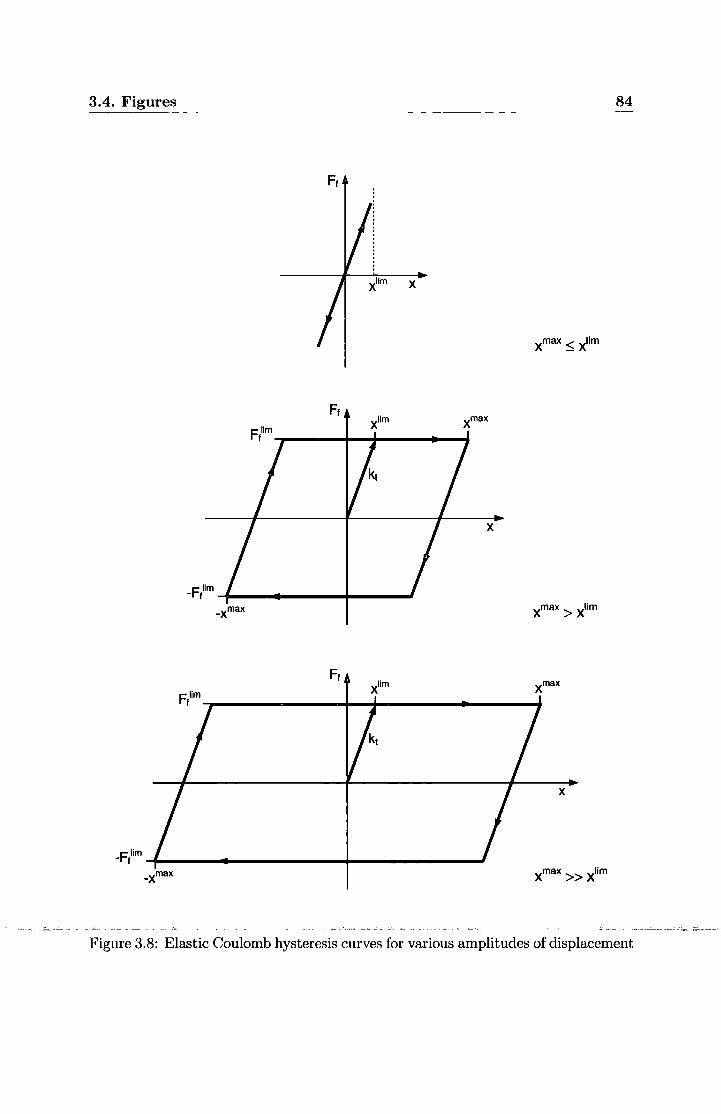
3.4. Figures 84

Fl

X

X

F lim - I ~--------------P-------J

Fl

X

F lim

- I ~--------~------------~----------------#

------=---- ___ .: ___ :;._.._..~-~

Figure 3.8: Elastic Coulomb hysteresis curves for various amplitudes of displacement

3.4. Figures 85

Elastic Coulomb friction work

elastic t: limit

~

Displacement amplitude

Elastic Coulomb friction damping ratio

Displacement amplitude

Figure 3.9: Variation of Elastic Coulomb friction work and damping ratio with

displacement amplitude

microslip gross slip

Tangential displacement, x

Figure 3.10: Microslip friction force during initial loading

3.4. Figures

X max

~-----:::::-'"--11----11- F/im

Figure 3.11: Microsli p friction hysteresis curve

Figure 3.12: Microslip friction work at slip limit

X max

J-.""7'""-----~1- Ftlim

X

X

Figure 3.13: Graphical representation of rnicroslip and sliding work

86

--~--------~

3.4. Figures

- - Microslip work

• • ·Slip Work

--Total work

,

, , , , , , , , , , ,

Displacement amplitude

Figure 3.14: Friction work predicted by the rnicroslip model

0

~ a: C) c ·a. E «< Q

Displacement amplitude

87

3.4. Figures 88

0.25 xlim 0.5 xlim J(im

Tangential displacement

Figure 3.16: Calculation of tangential stiffness using various positions on microslip

force curve

Chapter 4

Decoupled Forced Response

System

4.1 Overview of Methodology

Linearised decoupled methods provide a highly efficient frequency domain approach

for aeroelastic calculations. Fluid-structure interaction is dealt with in a loosely

coupled linear manner, assuming that mode shapes and natural frequencies of the

blade are not affected by aerodynamic loading. This assumption is valid for typical

compressor blades, which are of high density and stiffness and vibrate with low

amplitude. Efficient forced response methods based on the decoupled approach

are usually preferred over time-accurate methods due to the relative simplicity of

implementation, fast solution times and flexibility over choice of aerodynamic and

structural methods.

The methodology of the decoupled approach is illustrated in Figure 4.1. This

represents an open-loop system which requires only a single execution of the fluid

and structural calculations. The resonant vibration of a single mode is calculated

to give the steady-state blade vibration amplitude. Blade excitation is provided

by unsteady aerodynamic forces of the corresponding harmonic and the system is

__ SJtbj~c_t __ t_o ~:~,~r_QdY-IlJ!·IDiCJ:tpd __ s_tr,ucturaL damping.",.Blad(3_modeshapes,_are obtained __

from an FE modal analysis, one of which is selected for analysis and interpolated

onto the CFD mesh. The CFD analysis is simplified by decomposing the forcing

89

4.1. Overview of Methodology 90

and damping calculations into two separate parts to yield the aerodynamic forcing

function and the aerodynamic damping ratio. The forced response solution is then

calculated using a modal approach for the given forcing and damping terms to give

the resonant vibration amplitudes and stresses.

Finite Element Modal Analysis

Mode shapes and natural frequencies are provided by the modal analysis of a finite

element model of the blade structure. The FE software used in the analysis was

chosen to be Ansys, a typical commercial general-purpose package. The blade is

modelled as a single isolated blade, fully constrained at the root and assuming no

mechanical coupling between blades. Additionally, the method retains the capability

of modelling a bladed disk based on cyclic symmetry, where the complex modeshape

of a single blade segment is used. The stress stiffening effect of centrifugal loading

is accounted for by performing a preliminary static analysis at the specified engine

speed. Although less significant, steady fluid loading can be included in the static

analysis if desired by approximating the steady fluid pressures as a small series of

spanwise equivalent forces on the FE model. The result of the pre-stressing calcu­

lation is a modification to the system stiffness matrix used in the modal analysis.

The result of the modal analysis is a set of real mode eigenvectors, such that the

modal response of every point of the blade moves in phase, with relative amplitude

determined by the mode shape. If the blade is visualised to be repeated around the

annulus to represent the entire disc, then the modal response of each blade will be

seen to vibrate with a discrete interblade phase angle between neighbouring blades.

Whilst this approach is commonly accepted in the literature for unshrouded blades,

the decoupled approach is also capable of dealing with the analysis of shrouded

bladed disc assemblies utilising cyclic symmetry in the modal analysis. In this case,

a set of complex modes for the disc sector mode will result, representing a continuous

travelling wave of blade motion around the disc.

A single mode for investigation is selected from the set at the resonant crossing

point of interest on the Campbell diagram, dictating the mode, frequency and engine

speed. The modeshape is subsequently interpolated onto the CFD mesh as a distri-

4.1. Overview of Methodology 91

bution of real modeshape amplitudes over the aerofoil surfaces. The aerodynamic

boundary conditions are obtained from the performance map of the machine.

Aerodynamic Forcing

The unsteady aerodynamic excitation forces are obtained from either a single or

multi-stage CFD calculation which models the flow disturbances due to inlet distor­

tion or bladerow interaction. The forcing analysis is done with non-vibrating blades

to yield the unsteady harmonic pressure distribution over the blade surfaces due to

incoming flow disturbances. The unsteady pressure harmonic at the blade natural

frequency is integrated over the blade surfaces to provide the complex modal exci­

tation force. Forcing harmonics outside the natural frequency are assumed to have

an insignificant effect on the steady-state resonant response and are neglected. The

formulation of the modal excitation force is given later in Section 4.3.

Aerodynamic Damping

Aerodynamic damping is calculated based on the assumption that vibration-induced

pressures increase linearly with vibration amplitude. Whilst linear aerodynamic

damping behaviour for two transonic fan rotors has been observed by Li and He [74]

and Schmitt et al. [75], no evidence has yet been reported showing significant non­

linear damping for high frequency forced response cases with small blade deforma­

tion. The CFD damping calculation is performed on an isolated bladerow in clean

flow with the blade vibrating in the mode at the blade natural frequency. The am­

plitude of vibration is specified at a realistic level and the interblade phase angle is

determined by the wavelength of the aerodynamic disturbance. The induced har­

monic forces resulting from the blade vibrating in the fluid are calculated to give the

pressure distribution at the vibration harmonic. The harmonic pressures and blade

displacements are integrated over the blade surfaces to provide the work done on

the fluid by the blade over one vibratory cycle. An equivalent aerodynamic modal

. . . dampingiJ!·t.io is then~G.al~ulat~d_frpm th~ work, Q~~g Ql! theprinG.iple of_~quiva- . _ _ _____ _ •-~~--~--·-•--•~-'--. • • --"• • •••·~-- =• • T • • ·- '-. ·---"---·-•••------~~<---'·.-- --- ·---=----· --~ __ .:___ .• :-'""'- - • •"- ·-·-- ••··---------------......- -.•--.,..

lent viscous damping. The formulation for the aerodynamic damping calculation is

provided in Section 4. 3.

4.1. Overview of Methodology 92

Forced Response Solution

Once the aerodynamic forcing and damping terms are known, the forced response

is calculated very efficiently using a single DoF equation based on the CFD mesh.

Linear mechanical damping is included as a prescribed damping ratio, based on

the principal of equivalent viscous damping. Two methods of obtaining the forced

response solution are used: 1) the modal equation method; and 2) a new energy

method. The modal reduction method is the standard approach, involving the trans­

formation of physical variables into modal space before solving the modal equation.

The resulting modal amplitude is then expanded into physical space to give the

actual blade response. The energy method provides an alternative forced response

solution to the modal equation method and performs the calculations directly on the

CFD mesh using actual vibratory displacements. Here, the mode shape is directly

scaled to balance destabilising and stabilising work due to forcing and damping to

provide the blade motion at equilibrium .

.::: .. ..:...::__.~.---· -· -- . ---- -·-·· .

4.2. FE-CFD Mesh Interface 93

4.2 FE-CFD Mesh Interface

4.2.1 Problem Description

The modal displacements from the FE modal analysis are interpolated from the FE

mesh to the CFD mesh to allow the aerodynamic modal forcing to be calculated

using the fluid pressures on the CFD mesh. The calculation of modal forcing on

the CFD mesh requires only a single interpolation process for each mode under

consideration, providing an efficient forced response process. The alternative to this

approach would be to interpolate fluid pressures onto the FE mesh, where the modal

forcing would be calculated. The disadvantage of this alternative would be that fluid

pressures would need to be transferred to the FE mesh every time the CFD solver

is employed for the forcing and damping calculations. The calculation of modal

forcing on the CFD mesh is therefore a much simpler approach.

The FE-CFD interface is a major component of the forced response prediction

system, which must accurately interpolate the mode shape from the Ansys FE mesh

to the CFD mesh. The interface must be capable of interpolating with high accuracy,

whilst being robust enough to deal with the demands of industrial use. A large part

of the problem is due to the unstructured nature of FE meshes and the need to

facilitate the use of different structural element shapes. Whereas FE meshes may

take on the appearance of structured meshes, looking similar to structured CFD

meshes, the mesh data in Ansys is stored in an unstructured manner.

Further complications arise due to likelihood of slight variations between the

mesh geometries, resulting in non-coincident boundary surfaces of the two meshes.

The primary cause of this issue is due to the blade unrunning of the FE mesh, where

structural analysts "undo" the effects of centrifugal, static gas and temperature

loading of the blade to give the cold blade geometry. The cold shape is usually used

for subsequent structural analysis, leading to a significant difference in geometry

if the static deformation is not reapplied to the blade shape. The magnitude of

---· __ -'~~},s}ljJ!~Ee.~ce a~ .1~~ ~~!:' _c~':l21Lqf -'~!~ilaL~~e _ _!.~)~~~~%!~-t~i£~-~~1?~:"' ~e__c~ll~~ry __ --~~"'--'-"--~ differences in geometry are due to the planar nature of the element surfaces, which

do not conform exactly to the curved blade profile. Since the FE and CFD meshes

4.2. FE-CFD Mesh Interface 94

are not identical, the nodes of one mesh will not necessarily intersect the planar

surfaces of the other mesh. Such differences are relatively small, but the implication

on interpolation accuracy can be significant for low density meshes.

4.2.2 Metholology

A method of interpolation was developed to transfer the mode shape from an un­

structured FE mesh comprising of tetrahedral, hexahedral, prismatic and wedge el­

ements to a CFD structured mesh, based on the assumption of noncoincident mesh

boundary surfaces. The harmonic amplitudes of the mode shape are transferred to

the CFD mesh by 2D linear interpolation over the 3D FE mesh surface. For each

point on the CFD mesh boundary surface, a plane on the FE mesh boundary is

chosen. The plane is defined by three corner FE nodes on an external element face,

giving a single plane per triangular face and a selection of four planes per rectangu­

lar face, as shown in Figure 4.2. Forming a triangle, the three nodes are selected to

provide the closest centroid to the CFD point, thus defining the best interpolation

plane to provide maximum accuracy.

Interpolation of the mode shape components is performed at the orthogonal

projection of the CFD point onto the plane, as shown in Figure 4.3. The mode

shape data for the CFD point is taken at the projection point in order to minimise

errors caused by the mesh surfaces not coinciding. Methods of 3D interpolation are

expected to reduce accuracy by introducing errors for non-coincident surfaces.

Misalignment of the FE and CFD meshes is common due to differences in coordi­

nate systems, origins and orientation between the two meshes. Axial and rotational

alignment of the FE mesh to the CFD mesh is incorporated based on the specifi­

cation of reference nodes. The tip leading edge is normally taken as the reference

point, as it is often the most flexible part of the aerofoil with the highest strain

gradients, where interpolation accuracy is the most important.

At positions where the aero point lies close to an element-element boundary, noise

in the interpolated values can be seen due to the step change in plane orientation

from one element face to another. This effect is particularly noticeable in low­

density meshes or in areas of high modeshape gradients. The interpolation quality

4.2. FE-CFD Mesh Interface 95

is improved by averaging the interpolated data over the two adjacent elements if the

interpolation point lies within a specified proximity to an element-element boundary.

An additional source of error occurs when interpolation planes are not aligned

with the pressure and suction surfaces, such as the tip, leading and trailing edges

of typical, blunted FE meshes. Such surfaces lie normal to the desired interpolation

planes and can cause significant interpolation errors for low density FE meshes

around these regions. The errors are avoided by specifying the element and face

numbers on the FE mesh and preventing these surfaces from being used to define

interpolation planes. Fortunately, this edge effect does not provide concern for high­

density meshes and can be neglected.

CFD meshes incorporating tip clearance cells require further attention to define

the blade motion of the clearance cells above the blade tip. Since these cells lie

outside the FE mesh geometry, the axial and tangential mode shape components

are set equal to those at the tip. In order to prevent penetration of the blade mesh

into the casing, radial motion at the tip is linearly reduced through the clearance

cells to zero at the casing.

4.2.3 Mathematical Formulation

Orthogonal Projection onto Surface

As described above every combination of three adjacent FE mesh nodes is considered

to define the interpolation points used for each surface CFD grid point. The actual

three nodes chosen create a triangle with the closest centroid to the CFD point,

provided that the face is valid for interpolation. With the three points defining a

plane, 2D interpolation is performed at the orthogonal projection of the CFD point

on the plane to allow for small deviations of the CFD mesh surface from the FE

mesh surface.

Figure 4.4 shows three FE nodes A, Band C, defined relative to a global origin

by the position vectors a, b and c. The vectors of B and C relative to C are defined

as AB and AV. A vector ii noriri3J_clo~theABC.plane i~tootaineiftromtlle-cross ----'-'~-~-

4.2. FE-CFD Mesh Interface 96

product

ii=ABxAc ( 4.1)

The equation of the plane is therefore given by

(4.2)

where r is the position vector of an arbitrary point on the plane. The scalar A

is obtained from

(4.3)

Considering a point D positioned outside of the ABC plane, the orthogonal

projection of the point onto the plane defines a single point, E, such that the vector

DE is orthogonal to the plane. The parallel alignment of DE with the normal vector

ii gives the relationship

(4.4)

which is rewritten in the form

(4.5)

Substituting e into the plane equation ( 4.2) gives

(4.6)

which is expanded and rearranged to give

A- ( J. n) t = Iii 12 (4.7)

Substituting t into Equation 4.5 gives the orthogonal projection of the CFD

point, D, onto the plane, given by

____ (A-(d·n)) __ e = d + Iii 12 n (4.8)

4.2. FE-CFD Mesh Interface 97

Transformation into Local Coordinate System

Before interpolation takes place, the four planar points A,B,C and E are transformed

from the global X,Y,Z axes into a local i,j coordinate system. Figure 4.5 shows the

four points on the local i,j axis, together with the field variable ¢. The origin is

taken at point A and the i-axis is aligned with the vector AB, where the the unit

vector of the i-axis is defined in 30 space by

~ AB 'l=---

IABI (4.9)

The j-axis lies orthogonal to both the i-axis and the plane normal defined as

~ n xi

J=lfixil (4.10)

Points C and E are defined in the local 20 axes by taking the projection of each

point in the direction of each axis. The local 20 coordinates of each of the four

points is therefore given by

Interpolation Function

Aii = (0, 0)

Bij = (I A:B I, o) ni = ((AC · i), (AC · 3))

Eii = ((AE · i), (AE · J))

(4.11)

The linear interpolation function is calculated using the shape function of a 20

simplex triangular finite element based on an identical formulation to the ANSYS

element, which can be found in the ANSYS literature. The three modeshape OoFs

are interpolated using three individual interpolation functions where the linear in­

terpolation function for a single field value is given by

(4.12)

4.2. FE-CFD Mesh Interface

the positions of the three FE nodes A, B and C from the expressions

ct1 = (sAcPA + SBcPB + scc/Jc)/2A

ct2 = (tAcPA + tBcPB + tcc/Jc)/2A

ct3 = (uAcfJA + UBcPB + Ucc/Jc)/2A

where A is the area of the triangle ABC given by

A= ibjc 2

and the coefficients s, t and u are given by

SA= ~B)c

Sc = ~A]B- ~B]A

tB = jc- jA

tc = jA- jB

UA = ic- iB

Uc = ~B- ~A

98

( 4.13)

( 4.14)

(4.15)

Once a 1, a 2 and a 3 are known, the mode shape component ¢ is interpolated at

position E by solving Equation 4.12.

4.3. Modal Equation Method 99

4.3 Modal Equation Method

The modal equation method is based on the single-DoF modal equation outlined in

Section 3.2.2, where the forced response is obtained from the analytical solution of

the modal equation in the frequency domain.

Modal forcing is calculated on the CFD mesh, which avoids the need to inter­

polate fluid pressures from the CFD mesh to the FE mesh for each modal force

calculation. The modal force calculation is done using the modal displacements on

the CFD mesh which are interpolated only once from the FE mesh to the CFD mesh

in the manner described in Section 4.2.

The aerodynamic modal force is considered in terms of Lagrangian mechanics to

be the virtual work done by the fluid integrated over the blade surface. The ampli­

tude of translational displacement for each CFD mesh node on the blade surface is

defined in the axial, radial and azimuthal directions, which are combined in a single

vector { Xcfd} to provide all the nodal degrees of freedom of blade displacement. Each

nodal DoF is denoted by the index, j, giving a total, n, equal to three times the

number of surface nodes.

The vector of aerodynamic force amplitudes acting on the nodal DoFs is defined

as {F}, where the force amplitude acting on each individual DoF is given by

( 4.16)

Here, the force acting in the direction of the nodal DoF, j, is the product of the

fluid pressure, Pi, at the surface position of DoF j and Ai is the projection of the

effective nodal surface area in the direction of the DoF. The effective nodal surface

area is a summation of a proportion of the areas of neighboring surface cells.

The mesh displacements in each DoF are related to the mode shape in the same

manner as in Equation 3.9 to give

( 4.17)

for the single mode in question on the CFD mesh. The aerodynamic modal force

is then obtained from the summation of the virtual work done by the fluid at each

nodal DoF on the CFD mesh surface, given by

4.3. Modal Equation Method 100

( 4.18)

Considering the aerodynamic forces in terms of their real and imaginary compo­

nents, the modal force expression is written as

n

J = L { (ct>c1d)j (Fr + iFj~)} (4.19) j=l

The aerodynamic damping ratio (aero is calculated from the work done on the

blade by the fluid, obtained from the CFD damping calculation. Work is calculated

in physical terms by integrating the aerodynamic damping force distribution and

blade displacements over one vibratory cycle, using

n

wJJd = 1f L (Djxf- Dfx?rfd (4.20) j=l

where D'R and D~ are the complex components of the physical damping force vector

D and x'R and x~ are the complex components of the blade displacement vector x. However, if the blade motion in the damping calculation is specified to be entirely

real with zero imaginary component, the above work expression is reduced to

n

W cfd _ '""" (D~ ·)cfd d - 1f L..J j XJ (4.21)

j=l

Alternatively, if the modal damping force dis known, the work can be calculated

in modal space using

(4.22)

Values relating to the CFD damping calculation are based on the specified vi­

bration amplitude xcfd, and are denoted by the superscript cfd_ The aerodynamic

damping ratio is calculated from the work based on the principle of equivalent vis-

cous damping, wcJd

(aero = 21f:; ( ;cfd)2 ( 4.23)

The modal amplitude of the CFD damping calculation is simply given by the

-ratio bet~e~ll- the c:FJ5-'-blade motion xcfd and the mass~n~rmalised mode shape, ¢,

(4.24)

4.4. Energy Method 101

Mechanical damping, (mech, can be estimated or calculated separately and is added

to the aerodynamic damping to give total system damping (tot·

The modal equation (Equation 3.12) is analytically solved in the frequency do­

main to provide the solution of the modal equation for excitation at arbitrary fre­

quency, w, given by

lql = III J(w?- w2

)2 + (2(totWiw)

2 (4.25)

Since resonant vibration with excitation at the blade natural frequency, w = wi, is

only considered, the analytical solution to the modal equation reduces to,

lqfrl = 1{1 2wi (tot

(4.26)

yielding the magnitude of the modal amplitude of the forced response solution. The

resulting modal amplitude is then used to scale the modeshape by

(4.27)

transforming the modal amplitude into the physical response amplitudes of the

blade. Blade stresses and strains can be obtained in a similar manner, where modal

values from the FE mesh are scaled by the modal amplitude.

4.4 Energy Method

The energy method is a simple approach to obtaining the forced response solution

that requires less knowledge of structural dynamics than modal reduction method.

It eliminates the use of modal reduction theory for purely aeroelastic forced response

calculations. The method is based on an energy balance applied directly on the CFD

mesh in physical space. The major benefit of this approach is that the scale of the

mass-normalised mode shape is not required for the CFD calculations, therefore

eliminating a potential practical issue. Instead, modeshapes can be scaled freely,

- --disregarding- original modeshape~scales-arid_cunits·,c-allowing-modeshapecfiles-to be­

passed freely between analysts and designers with minimal communication about

how the modeshapes were created.

-------.-----·-~

4.4. Energy Method 102

Considering a system undergoing forced vibration in terms of work transfer,

steady-state vibration occurs at the amplitude where the forcing work ( destabilising)

applied to the blade per cycle balances the dissipated damping work (stabilising).

Based on a linear increase of forcing work with vibration amplitude and a quadratic

increase of damping work, a single point of equilibrium can be found, giving the

forced response solution, as shown in Figure 4.6. Firstly, forcing work and damping

work are calculated at a specified amplitude of vibration, then the work values are

scaled to achieve equilibrium to provide the vibration amplitude at the point of

steady-state forced vibration.

The calculation of the damping work is the most straightforward task, knowing

that the relative phase between the blade motion and damping forces remains con­

stant for a given vibration amplitude. The damping work is simply taken as the

value given by the CFD damping calculation using Equation 4.21.

Forcing work is calculated knowing that: 1) aerodynamic excitation forces remain

fixed and are not affected by blade motion; and 2) the vibration will lag the force

distribution with the phase providing the maximum destabilising effect. For example,

the response of a simple spring-mass system undergoing resonant forced vibration

will lag the excitation force by exactly goo. In other words, the blade motion lags

the forcing by the angle providing the maximum work to the blade. Similarly, for

a multi-DoF system undergoing resonance from an excitation force distribution,

the modeshape lags the forces by the phase angle providing the maximum work.

However, since individual forces in the distribution may be out of phase with one-­

another, no datum forcing phase is defined, so the response phase can not be defined

by a goo lag. Instead, the response phase is defined at the angle providing the

maximum forcing work. As illustrated in Figure 4.7, the forcing work follows a

sinusoidal variation with vibration phase. A simple iterative approach calculates

the work done on the blade at discrete angles varying between 0 and 27r to obtain

the work done for all possible phase angles. The forcing work is simply taken to be

the maximum value.

Once the aerodynamic forcing and damping work is known, the point of equilib­

rium at the amplitude of steady-state vibration is found by scaling the linear forcing

4.4. Energy Method 103

term and quadratic damping term to yield the forced response solution. Firstly aero­

dynamic forcing work, W 1, and aerodynamic damping work, Wad, over one cycle are

expressed as functions of modal amplitude, where forcing work is linearly propor­

tional to modal amplitude and damping work is proportional to the square of modal

amplitude. Representing the relationships using constant coefficients {31 and f3ad for

the forcing and damping terms respectively, gives

However, all work calculations are initially based on the scale of the blade motion

used in the CFD damping calculation, where { xcfd} is the displacement amplitude

vector of the CFD mesh. Any value corresponding to this vibration scale is denoted

by the superscript cfd, and the above work expressions are written as

w.:fd = /3 qcfd. wcfd = /3 (qcfd)2 f f ' ad ad ·

Secondly, mechanical damping is included as

where the work is calculated from the structural damping ratio , (mech, at the same

modal amplitude by

W cfd _ 2 I" 2 ( cfd)2 m:l - 1r'-,mech W q ·

If the actual value of qcfd is unknown at this stage, it can be calculated by comparing

the blade motion of the CFD mesh in the damping calculation to the original mass­

normalised eigenvector for any DoF, j, of the blade using

cfd X·

q cfd = _J_ c/>j .

The work coefficients, fJJ, f3ad and !3md can be used to determine the work at arbitrary

vibration amplitude, in particular, the equilibrium amplitude, qeq, of the forced

response solution;

wcfd weq wcfd weq w.:fd weq

/3- f_ f ,q ad ad/3 md md

f - qcfd - qeq ' fJad = ( qcfd)2 = ( qeq)2' md = ( qcfd)2 = ( qeq)2 · (4.28)

4.4. Energy Method 104

The forcing and damping work is then scaled to find the point of equilibrium,

where destabilising work input equals stabilising work dissipated, given by

-weq = weq + weq f ad md•

or in terms of vibration amplitude by substituting the relationships from Equa­

tion 4.28,

Factorising for qeq and substituting f3 terms for the expressions of the known values

of work (Equation 4.28) gives

wcfd f wad wmd eq ---

(

cfd cfd )

( qcfd)2 + ( qcfd? q ' qcfd

when rearranged gives

(

-wcfd ) eq_ f cfd q - wcJd + wcJd q

ad md

Expressing the equilibrium blade motion as

(4.29)

allows the equilibrium modal amplitude to be eliminated from the above expression,

where the energy balance equation expressed in terms of work, i.e.

(

wcfd ) { Xeq} = - f {xcfd}

wcJd + wcJd ad md

(4.30)

Here, the actual blade motion of the CFD mesh used in the damping calculation

is scaled to yield the harmonic amplitudes of the response solution. If mechanical

damping is neglected, the calculation requires no knowledge of the eigenvector scale.

Where mechanical damping is included, the eigenvector scale is needed but the

method still avoids the use of modal algebra, providing a useful alternative to the

modal equation method.

4.5. Figures 105

4.5 Figures

Figure 4.1: Decou pled forced response system

A B A B

N0 D . C D . . C • Centroid

Figure 4.2: Possible interpolation planes for a rectangular FE element face

FE nodes

Figure 4.3: 2D interpolation at projection onto FE mesh surface

4.5. Figures

-n

A

CFD D point

B

Figure 4.4: Calculation of orthogonal projection point

106

Figure 4.5: Transformation of interpolation points into local 2D geometrical axis

system

Vibration Amplitude

' ' ' ' !response !amplitude ' ' :

Figure 4.6: Equilibrium of forcing and damping work

4.5. Figures

\

aero forces \,

I mag

(fixed) \\,

---- ~\

blade motion (all DoF in phase)

hase Real

107

Work

W ctd F::~r:_Cif!g_~ork I I

I--+--~-~---Vibration Phase

Figure 4. 7: Response phase for maximum forcing work

Chapter 5

Verification of the Decoupled

System

5.1 Introduction

The NASA Rotor 67 transonic fan rotor was used as the preliminary case study

during the development of the components of the forced response system. The rotor

provides a relatively simple case to demonstrate the forced response methodologies,

involving only a single bladerow calculation. Four modes are considered in sepa­

rate forced response analyses to demonstrate the implementation of the decoupled

method and provide a basis for further investigation of alternative fluid-structure

coupling strategies.

The system is evaluated for a challenging industrial study of a Siemens 3-stage

transonic test compressor, where the forced response predictions of three high fre­

quency crossing points on the Campbell diagram are compared with strain gauge

test data. This case offers a good benchmark for the forced response system, provid­

ing many of the difficulties encountered in an industrial environment, whilst allowing

the validation of predictions against engine test data. This case study has been done

in cooperation with Siemens, who assisted in the analysis and provided test data.

108

5.2. NASA Rotor 67 Transonic Fan 109

5.2 NASA Rotor 67 Transonic Fan

5.2.1 Case Description

The NASA Rotor 67 transonic fan is typical of modern low-aspect ratio transonic

fan design and consists of 22 unshrouded blades of 93mm chord length at tip. The

details of the rotor aerodynamics are available in the public domain and there have

been several published studies on its unsteady aerodynamic and aeromechanical per­

formance. Publications on the aero mechanical analysis of NASA Rotor 67 have in­

cluded the flutter calculations of Marshall and Imregun [5] and Srivastava et al. [147]

based on time-accurate CFD codes. The fan is designed to produce a total pressure

ratio of 1.63 for a mass flow rate of 32.25 kg/ sec with a tip inlet relative Mach

number of 1.38 at the design point of speed 16,043 rpm.

For each of the four resonant operating conditions investigated, blade excitation

is provided by hypothetical inlet distortions to simulate inlet flow conditions typi­

cally encountered in inlet distortion and bladerow interaction problems. The number

of nodal diameters of the distortions are chosen to provide excitation for each mode

at crossing points close to 100% design speed. The aim is to provide forced response

calculations for a fairly wide range of resonant conditions from the fundamental

modes typical of inlet distortion cases, to a high frequency mode typical of bladerow

interaction problems. The crossing points of the 1st and 2nd bending, 1st torsion

and the rh modes with the 2nd, 5th, rh and 15th excitation orders, respectively, are

investigated. To illustrate the physical representation of this case study, the rotor

geometry with a 2-node inlet flow distortion pattern is shown in Figure 5.1.

Structural Modelling

Due to the fact that only aerodynamic data was available, the FE mesh was con­

structed based on the geometry of the CFD mesh, giving a model comprising of 806

quadratic 20-node brick elements. The FE and CFD meshes can be seen later in this

. J~~~tiQ!l. inJ~)gw:e 5.4. S_i!lc~t_ll,(l.ge()pi~tu.cPf tll,~ .blag~tf.QQt~W~cno_t!<~o~n,tl!e bla.de~ ~--.c.=.cc..:.,_c .

was modelled as an aerofoil cantilevered at the hub. The material properties of the

blade were not known and typical properties for titanium were assumed (density,

5.2. NASA Rotor 67 Transonic Fan 110

4110 kgjm3; Young's modulus of elasticity, 125 CPa, Poisson's ratio, 0.27).

The stress stiffening effect of the centrifugal loading is incorporated based on a

static analysis at 100% speed. For simplicity, the influence of steady gas loads on

the modal solution are assumed to be negligible. The blade static twisting effect did

not need to be included since the FE mesh already conformed to the hot running

shape of the CFD mesh.

CFD Modelling

The fluid H-mesh consisting of 110x25x29 results in a single-passage 3-D compu­

tational domain of approximately 73k cells, on which the linearised Navier-Stokes

equations are solved in the frequency domain. A blade-blade view of the mesh can

be seen in Figure 5.5 and a portion of the mesh over the blade surface is shown in

Figure 5.4. For reasons of convenience, the blade count is modified from 22 to 21

in order to verify results against the previous work of Li and He [74]. Since a single

passage approach is used in the CFD analysis, no computational benefits are gained

from this change.

Flow conditions are taken close to the design load and the strength of the inlet

distortion is specified by perturbing the steady flow solution at the inlet plane.

Once the steady solution is achieved, a perturbation of the axial velocity at the inlet

plane is prescribed. Assuming that all other flow conditions remain unchanged, the

density is adjusted accordingly to ensure constant static pressure at the inlet. The

strength of the axial velocity perturbation is set such that the relative dynamic

head perturbation at inlet is at a realistic level of approximately 10%. The forcing

calculation is performed through a single passage of non-vibrating blades subject to

the prescribed inlet distortion to yield the resulting unsteady pressure distribution

over the blade surfaces caused by the incoming flow disturbances.

The damping calculation is carried out with vibration in the specified modes,

with the modeshapes scaled to provide a leading edge tip deflection equal to 1% blade

chord. In each damping calculation, the blade is set to oscillate with fixed amplitude _: :;_,_-~_,~ -•~...:.·-"--------- • ~----- •.:_·.~·- -- • e" .··_ =--~""··:.· ' -·-- .___..:::...::.' :::" ",_, ,_:_::.___,~ .. ::::: ____ ;_,;,'-'.,.:2"_=·-: __ ,____:._:_::_- _..:.,;-~---:....:_ "•_:!_..:. :_ ~-;- ·_:::_:_:: -"'_:=-=--.-=.--'- -· .J .-.:--~ .=..: .• :.· '"'- •;o,:_•'-' "--·- -. --·~---=-~- .,_:C--o..;·,~~--

and phase, subject to clean, undisturbed inlet flow. The resulting unsteady pressure

distribution is integrated over the moving pressure and suction surfaces to provide

5.2. NASA Rotor 67 Transonic Fan 111

Mode Frequency (Hz) Description

1 601.0 1st flap

2 1307.9 2nd flap

3 1913.2 1st torsion

4 2740.6 1st edgewise

5 3148.6 Combined

6 3520.0 Combined

7 4198.4 Combined

Table 5.1: Natural frequencies and modeshapes

the work done on the blade.

5.2.2 Results

Modal Analysis

The modal analysis yielded the first seven natural frequencies listed in Table 5.1 and

four modes of interest are illustrated in Figure 5.2. The predicted frequencies were

compared to the work of Marshall, 1996, and were found to differ slightly, as shown

in Figure 5.3. The almost linear difference does not cause concern because many of

the parameters used by Marshall are unspecified. The quality of the FE mesh was

confirmed by checking the sensitivity of the natural frequencies to mesh density and

element type. The results were compared against the frequencies of two additional

models constructed with 195 and 806 linear 8-node brick elements. The effects of

mesh refinement were found to be negligible, indicating the fidelity of the mesh.

The interpolation of the modeshape onto the CFD mesh was verified by super­

imposing the modeshape contour plots of the two meshes using Tecplot. Excellent

interpolation accuracy was observed, and no visible difference was observed between

the two meshes. The contour plots of the mode 7 axial component are provided in

_figu!:~ __ 5.4.lt sho!lld be not~d __ th~t t~ iD.J;em_ola:tiqn __ ~CUJ.:!l-CY- w~ expe~t~dtQ_g~e_

very high between the two meshes, since the blade shapes are identical and a high

proportion of nodes coincide.

5.2. NASA Rotor 67 Transonic Fan 112

Mode Nodal Vx Distortion Engine Modal No. Diameters Amplitude Speed(%) Force

1 2 1% 112.4% 13.8

2 5 5% 97.8% 10.6

3 7 15% 102.2% 41.6

7 15 15% 104.7% 15.4

Table 5.2: Target inlet conditions and solution modal force

Aerodynamic Forcing

The first step in the aerodynamic analysis yielded the steady flow solution, on which

the unsteady calculations were based. A contour plot of the Mach number and

entropy at 33% span is provided in Figure 5.5. A thick boundary layer can be seen

due to the relatively low mesh resolution, the effects of which are not a significant

concern in this case.

The prescribed "target" inlet conditions for the forcing calculation are given in

Table 5.2, representing light, but realistic cases. As mentioned in Section 3.1.4,

only the stagnation pressure, stagnation temperature and flow angle are specified

at the inlet and it is not possible to prescribe all inlet properties. Target properties

such as density and velocity are specified as initial conditions at the start of the

calculation but are subject to change during the course of the solution. Contour plots

of the 7-node inlet axial velocity and density are shown in Figure 5.6 for the steady

solution, target inlet conditions and actual inlet conditions achieved at solution. It

can be seen that the solution inlet profile differs from the desired prescribed inlet

conditions of 15% axial velocity. Smearing of the velocity and density perturbations

can be seen towards the tip, together with a reduction in perturbation amplitude.

In addition, Figure 5. 7 shows that high pressure amplitudes have developed around

the tip, caused by upstream travelling pressure disturbances. The resulting modal

excitation force for each distortion case is given in Table 5.2.

5.2. NASA Rotor 67 Transonic Fan 113

Mode Frequency Modal Work Damping No. (Hz) Amplitude (Jjcycle) Ratio

1 601.0 1.212 x w-4 -0.00486 0.369%

2 1307.9 8.657 x w-5 -0.00415 0.130%

3 1913.2 4.860 x w-5 -0.0119 0.568%

7 4198.4 4.073 x w-5 -0.0111 0.153%

Table 5.3: Aerodynamic damping

Aerodynamic Damping

The solutions of the damping calculations at the specified modal amplitudes are

summarised in Table 5.3, where the damping ratio is given by Equation 4.23. It can

be seen that aerodynamic damping is very dependent on modeshape, with relatively

high damping of the 1st bending and torsion modes. This behaviour is typical for

turbomachinery blades and the predicted trend agrees fairly well with Kielb and

Imregun [9] for an unshrouded damperless blade. Figure 5.8 shows the imaginary

component of the damping force distribution over the pressure surface induced by

blade motion in the 1st torsion mode and the work done over one cycle due to motion

in the axial direction. Negative work represents areas of positive damping. This

representation of damping forces can provide a useful tool for blade designers who

wish to fine-tune aerofoil designs to maximise aerodynamic damping for a particular

mode.

Forced Response Solution

The modal equation (4.26) is solved for each crossing point in Table 5.4 using the

aerodynamic forcing and damping values obtained above. The mode 3 calculation is

repeated using a mechanical damping ratio of 0.1% for comparison with the energy

method below. The resulting response of each mode is expressed in terms of modal

amplitude and tip leading edge amplitude normalised to chord length.

The solutions of the energy equation ( 4.30) are provided in Table 5.5, where it

can be seen that the energy method produces identical results to the modal solution

5.3. Siemens Three-Stage Transonic Compressor 114

Mode 171 (aero (mech qfr Tip L.E. Amp. No. (%chord)

1 13.8 0.369% 0 1.131 x w-4 1.096

2 10.6 0.130% 0 6.011 x w-5 0.691

3 41.6 0.568% 0 2.532 x w-5 0.521

3 41.6 0.568% 0.1% 2.153 x w-5 0.443

7 15.4 0.153% 0 0.121 x w-5 0.164

Table 5.4: Forced response solutions using modal method

Mode (mech wcJd

I wcfd

ad wcfit

md Tip L.E. Amp. No. (Jjcycle) (J /cycle) (J /cycle) (%chord)

1 0% 0.005265 -0.00486 0 1.096

2 0% 0.02876 -0.00415 0 0.691

3 0% 0.00635 -0.0122 0 0.521

3 0.1% 0.00635 -0.0122 -0.00214 0.443

7 0% 0.00197 -0.00111 0 0.164

Table 5.5: Forced response solutions using energy method

shown in Table 5.4. To verify the energy method used with mechanical damping,

the mode 3 calculation is repeated with an assumed damping ratio of 0.1 %, giving

full agreement with the modal solution. The energy equation has, therefore, been

shown to produce identical results to the modal method for resonant vibration cases

both with and without the effect of mechanical damping.

5.3 Siemens Three-Stage Transonic Compressor

5.3.1 Case Description

The Siemens three-stage transonic test compressor shown in Figure 5.9 is a modern

·liigh ~performance niooerii-machiiie,~aeliverrlig;c~tliiglicspecifi'E1low witli a: mass flow--~"--·· oc_.='--- ~-- ·

rate of 26.3kg /sec and a pressure ratio of 3:1 at a rotating speed of 18, 650 rpm.

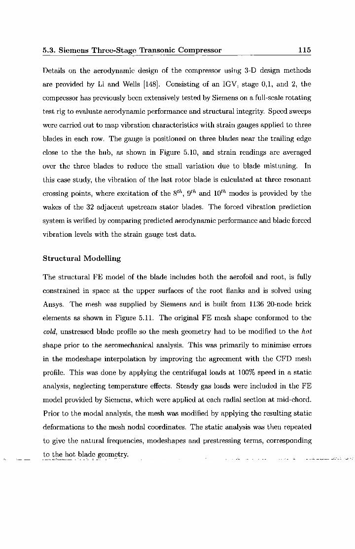
5.3. Siemens Three-Stage Transonic Compressor 115

Details on the aerodynamic design of the compressor using 3-D design methods

are provided by Li and Wells [148]. Consisting of an IGV, stage 0,1, and 2, the

compressor has previously been extensively tested by Siemens on a full-scale rotating

test rig to evaluate aerodynamic performance and structural integrity. Speed sweeps

were carried out to map vibration characteristics with strain gauges applied to three

blades in each row. The gauge is positioned on three blades near the trailing edge

close to the the hub, as shown in Figure 5.10, and strain readings are averaged

over the three blades to reduce the small variation due to blade mistuning. In

this case study, the vibration of the last rotor blade is calculated at three resonant

crossing points, where excitation of the 8th, gth and lOth modes is provided by the

wakes of the 32 adjacent upstream stator blades. The forced vibration prediction

system is verified by comparing predicted aerodynamic performance and blade forced

vibration levels with the strain gauge test data.

Structural Modelling

The structural FE model of the blade includes both the aerofoil and root, is fully

constrained in space at the upper surfaces of the root flanks and is solved using

Ansys. The mesh was supplied by Siemens and is built from 1136 20-node brick

elements as shown in Figure 5.11. The original FE mesh shape conformed to the

cold, unstressed blade profile so the mesh geometry had to be modified to the hot

shape prior to the aeromechanical analysis. This was primarily to minimise errors

in the modeshape interpolation by improving the agreement with the CFD mesh

profile. This was done by applying the centrifugal loads at 100% speed in a static

analysis, neglecting temperature effects. Steady gas loads were included in the FE

model provided by Siemens, which were applied at each radial section at mid-chord.

Prior to the modal analysis, the mesh was modified by applying the resulting static

deformations to the mesh nodal coordinates. The static analysis was then repeated

to give the natural frequencies, modeshapes and prestressing terms, corresponding

_0_ !~~~~_9t ~l8;de geom~try. _ _ _ _ __ _ _ _ _ "" _c..c- -'--'-'==c.

5.3. Siemens Three-Stage Transonic Compressor 116

Modeshape Interpolation

The interpolation of the modeshape onto the CFD mesh poses a challenging problem,

where the interpolation of high-order modeshapes from a low resolution FE mesh

raises several issues, including mesh alignment, shape mismatch, low mesh density

and high modeshape gradients. Axial rotational and translational alignment due to

differences in the coordinate systems is done by specifying the tip leading edge node

indices of the both meshes, then bringing the FE reference node into alignment with

the CFD node. An additional axial offset is specified to account for the blunted

leading and trailing edges of the FE mesh. Aligning the meshes at the tip leading

edge ensures the best possible interpolation accuracy around this critical region with

highly localised blade motion.

Modeshapes are interpolated onto the tip clearance region of the CFD mesh,

as outlined in Section 4.2.2. Axial and tangential motion of the clearance cells are

set equal to blade tip and radial motion is linearly reduced to zero at the casing

boundary.

CFD Modelling

The CFD calculations for the 3-stage compressor were performed by Dr. Wei Ning,

Siemens, hence only a brief overview of the CFD calculations is provided herein.

The steady solution is firstly obtained from a multi-stage analysis through the seven

bladerows of the 3-stage machine, upon which, the unsteady flow is calculated from

the linearised Navier-Stokes equations. Each blade passage is modelled by about

200,000 mesh points, giving around 1.5 million mesh points for the complete model.

The forcing calculation is done through the 7 bladerows to provide the wakes passing

through the rotor passages, and the damping calculation involves a single bladerow

analysis.

5.3. Siemens Three-Stage Transonic Compressor 117

Mode 8 9 10

Frequency (Hz) 8556 8823 10100

Table 5.6: Natural frequencies

5.3.2 Results

Modal Analysis

The calculated natural frequencies of modes 8, 9 and 10 at 100% speed are given in

Table 5.6. The FE analysis was repeated at zero rotational speed and the Campbell

diagram shown in Figure 5.12 was constructed around the crossing points of the

32-E.O. line with the three modes of interest. Here, it can be seen that the 32-

E.O. interference from the upstream stator row intersects blade modes 8,9, and 10

at between 70% and 105% engine speed. Included in Figure 5.12 are the modal

frequencies of the strain gauge measurements, where it can be seen that the FE

modal analysis agrees reasonably well with the test data. As shown in Figure 5.13,

the three modes are mainly aerofoil-dominated modes with very little motion at the

hub and root, particularly for mode 9.

Modeshape Interpolation

A comparison between the original and interpolated axial component of the mode­

shape data is given in Figure 5.14. The interpolation accuracy is very high for all

three modes, regardless of a small degree of shape mismatch caused by the 'unload­

ing' and 'reloading' of the FE mesh geometry. Whereas the tip L.E. of both meshes

are perfectly aligned, the slight difference in blade twist between the meshes causes a

misalignment at the tip T.E. of approximately half the blade thickness. In addition

to verifying the interpolation accuracy for a challenging case, this also demonstrates

that the mesh interface is very robust to differences in mesh shape.

The steady flow calculations are compared with measurements at 90% and 100%

design speed in Figure 5.15, showing a good overall level of agreement between

5.3. Siemens Three-Stage Transonic Compressor 118

Mode 8 Mode 9 Mode 10

(tot 0.35% 0.17% 0.13%

(aero 0.11% 0.17% 0.13%

(mech 0.24% Negligible Negligible

Table 5. 7: Aerodynamic and mechanical damping ratios

prediction and measurements, but with a slight under-prediction in efficiency. The

resulting modal force and damping ratio from the CFD forcing and damping calcu­

lations are provided in Table 5.8.

To compare aerodynamic with mechanical damping, the total system damping,

(tot. was obtained from the test data using the half-power rule on the strain gauge

frequency response. Mechanical damping, (mech, is then taken as the difference

between system and aerodynamic damping, (aero· The comparison in Table 5. 7 shows

significant mechanical damping for mode 8 and negligible mechanical damping for

modes 9 and 10. The mechanical damping for mode 8 is thought to be primarily due

to friction at the blade root-disk interface, where a greater degree of root motion is

apparent from the modeshape contours. The very small levels of displacement near

the root for modes 9 and 10 explain the negligible damping for those modes.

Forced Response Solution

The resulting predicted modal force is used together with the predicted aerody­

namic damping and mechanical damping to calculate the resonant displacements

and strains for each mode. Table 5.8 lists the modal forcing, 171, total modal sys­

tem damping ratios, (tot. and the resulting forced response modal amplitude, qfr.

The modal solution was verified by checking the results against the energy method

solution, which gave identical responses. Included in the table is the relative er­

ror between predicted strains at the gauge position and the measured strain gauge

readings.

---o_ ------'------·--- ---- - The-m.oae- 8 arid 10 J>reaictiorissnow-verfgood -agreement: -Tlie~greateraisagree=- ~----

ment of mode 9 is believed to be due to the poor positioning of the strain gauge for

5.4. Conclusions 119

Mode Modal Force Damping Ratio Modal Amp. Relative Error No. (171) ((tot) (qfr) with Test

8 11.17 0.35% 5.51 x 10-7 8%

9 5.25 0.17% 5.02 x 10-7 65%

10 1.79 0.13% 1.11 x 10-7 4%

Table 5.8: Forced response solutions

that particular mode (shown in Figure 5.10), raising the question about the accuracy

of the mode 9 measurement. Originally positioned to capture the low order modes,

the gauge is positioned over a region of high modeshape gradient, as visible in the

mode shape contour plots in Figure 5.13. This causes a significant change in strain

over the area of the gauge, reducing the accuracy of the strain measurement. Ad­

ditionally, the strain gauge sensitivity factor, defined as the percentage of the local

strain at the gauge location to the maximum strain on the blade, is at a satisfactory

level of around 25% for mode 8, but is lower than desired for modes 9 and 10 due

to the low modal displacements towards the blade root.

5.4 Conclusions

5.4.1 NASA Rotor 67 Transonic Fan

A case study of the NASA Rotor 67 transonic fan has been reported, providing

a detailed demonstration of the complete forced response prediction system, and a

basis for the validation of the individual system components. The resonant vibration

of a range of modes is modelled with excitation provided by inlet distortions of low

and high frequencies to simulate realistic aerodynamic conditions encountered in

inlet distortion and bladerow interaction problems.

The FE modal analysis was undertaken with ANSYS using a 20-node brick

element mesh, constrained as a cantilevered aerofoil. Mode shapes and natural

frequencies are in reasonable agreement with published FE results and were found

to be adequately insensitive to mesh resolution.

5.4. Conclusions 120

Very high mode shape interpolation accuracy of the FE-CFD interface was ob­

served by comparing the contours of the original mode shapes on the FE mesh with

interpolated mode shapes on the CFD mesh.

The CFD steady solution is in agreement with previous work of the research

group by Li and He [74]. The inlet axial velocity and density distortions show a

smearing of the target distortion pattern, which is likely to be due to upstream­

travelling pressure waves. Aerodynamic damping calculated with blade motion in

each of the prescribed modes shows reasonable damping predictions.

The decoupled forced response solution has been successfully implemented in

a hypothetical but realistic case study. Forced vibration levels are within the ex­

pected order of magnitude, with the l 8 t bending mode giving a tip deflection of

approximately 1% chord.

The energy method is shown to provide identical results to the solution of the

modal equation when implemented both with and without mechanical damping,

demonstrating that the energy method provides a simple alternative to the solution

of the modal equation.

5.4.2 Siemens Three-Stage Transonic Compressor

The forced response system was applied to predict the vibration of the last stage

rotor of the Siemens three-stage transonic test compressor, caused by high frequency

interference from the upstream stator wakes at three crossing points on the Campbell

diagram. The system was validated by comparing predictions with aerodynamic

performance and strain gauge measurements from a full-scale rotating engine test.

The FE mesh includes the root and originally conformed to the cold, unloaded

shape. The mesh geometry was modified to match the hot, running shape based

on a static FE analysis incorporating centrifugal and steady gas loads. Agreement

in shape with the hot shape of the CFD mesh boundary was significantly improved

but a visible difference in tip twist remained. Predicted natural frequencies agreed

_ --~------'- welLwith.the measuredo blade frequencies.~~--- __ , ____ , ---~ _ _ _ _ ____ ---'----"-------~-=c.-

The modeshape interpolation for this industrial case provided a challenging prob-

lem, raising several practical issues, including mesh alignment, shape mismatch, low

5.4. Conclusions 121

mesh density and high mode shape gradients. Mode shapes were interpolated with

very high accuracy, overcoming the above complications. The interpolation method

was found to be surprisingly robust to mismatching meshes, where a large difference

in twist at the tip trailing edge caused no reduction in interpolation accuracy.

The 7-bladerow CFD calculation predicted the compressor performance maps

with good agreement with measured data, but gave a slight under-prediction of effi­

ciency. Predicted aerodynamic damping compared well with total measured system

damping, for modes 9 and 10. An under-prediction in damping for mode 9 suggests

significant mechanical damping due to a greater amount of movement at the root

providing friction damping at the root-disk interface.

The forced response strain predictions, calculated using system damping, agreed

within 10% of strain gauge readings for modes 8 and 10. The mode 9 result gave

a discrepancy of 65%. However, the mode 9 result is inconclusive due to the poor

positioning of the strain gauge for that mode.

It has been demonstrated that the forced response system is capable of predicting

resonant strains with acceptable accuracy. The high efficiency of the unsteady multi­

stage calculation enables the the system to be used routinely in the blade design

process to tackle aeromechanical issues, where the turnaround time for each mode

is a few hours on a single processor workstation.

5.5. Figures 122

5.5 Figures

Figure 5.1: NASA Rotor 67 fan rotor geometry with contour plot of 2-node inlet

distortion

Figure 5.2: Mode shape axial components

5.5. Figures

8000 ~--------------------------------~

7000

6000

•Marshall (1996)

IJ26x31 Quadratic Grid

1!1 26x31 Linear Grid N' c 5000 -j--l~l!l~1~3x~1~5_.::L~in~ea~r_::G:'_'_n~·d _ _j------ --lr---.->-

~ 4000 -1------------------, :::J

w 3000 +--------------­u.. 2000 +------------

2 3 4 5 6 7 8

Mode

123

Figure 5.3: Comparison of natural frequencies with results of Marshall, 1996

ux 15 0.000765307 14 0 .000672379 13 0.000579452 12 0 .000486524 11 0.000393596 10 0.000300668 9 0.00020774 8 0.000114812 7 2.18844E-05 6 -7.10434E-05 5 -0.000163971 4 -0.000256899 3 -0.000349827 2 -0.000442755 1 -0.000535683

Figure 5.4: Comparison of original and interpolated modeshape (axial component)

5.5. Figures 124

Number

Figure 5.5: CFD mesh section and steady solution plotted at %span)

5.5. Figures

Target Axial Velocity Perturbation

VX!J 188.345 179.883 171.421 162.958 154.496 146.034 137.572 129.109 120.647 112.185

UWAKEpert 11 .5661 8.98958 6.41307 3.83656 1.26005

-1.31645 -3.89296 ~.46947 -9.04598 -11 .6225

Solution Axial Velocity Perturbation

VX.,ert 15.5198 12.0439 8.56809 5.09225 1.61642

-1 .85942 ~.33525

~.81109

-12.2869 -15.7628

125

Steady Solution Density

Target Density Perturbation

Solution Density Perturbation

Figure 5.6: Inlet axial velocity and density distort ion

RO,a 1.08792 1.08056 1.07319 1.06583 1.05846 1.051 1 1.04373 1.03637 1.029 1.02164

RWAKEpert 0.0168414 0.0130894 0.00933752 0.00558559 0.00183366 ~.00191826 ~ .00567019

~ .00942212

~.013174 ~ .016926

RO ert 0.0231283 0.0178693 0.0126103 0.00735126 0.00209226 ~.00316675 -0.00842576 -0.0136848 -0.0189438 -0.0242028

5.5. Figures

p 429.601 326.166 222.73 119.295 15.859

-87.5766 -1 91.012 -294.448 -397.883

Figure 5. 7: Inlet total pressure perturbation of solution

Axial Force Distribution (lmag Component)

Fx(lm) 0.0236987 0.0164939 0.00928915 0.00208435

-0.00512044 -0.0123252 -0.01953 -0.0267348 -0.0339396 -0.0411444

Work

126

Work X 5.67601 E-06 7.63908E-07

-4.14819E-06 -9.06029E-06 -1.39724E-05 -1.88845E-05 -2.37966E-05 -2.87087E-05 -3.36208E-05 -3.85329E-05

Figure 5.8: Mode 3, imaginary component of axial force and work in axial direction

5.5. Figures

Figure 5.9: Cross section of Siemens 3-stage transonic compressor

Gauge position

Figure 5.10: Strain gauge location on Rotor 2 blade

_l_j

u

I-- 1----1-

~ J-=ftl-117

I I

I;;

Figure 5.11: FE mesh of compressor blade

127

5.5. Figures

N' J: -->-u c Q) ::I C" ~ LL

Marks from strain gauge measurements 70%

Mode 10

Mode 9

ModeS

SPEED (RPM)

128

100%

32EO

Figure 5.12: Campbell diagram around 32E.O. crossing point with modes 8, 9 and

10

Mode 8 Mode 9 Mode 10

Figure 5.13: Axial modeshape components of modes 8,9 and 10

5.5. Figures 129

FE mesh

Figure 5.14: Comparison of original and interpolated modeshape for mode 9 axial

component

--·

0 Measurement

""""""'"""""""""" -·---l

0 "iii a: Q)

:; Ul Ul

~ a.. (ij 0 1-

-+-Prediction ~ )

t

0~ ~

~ H ......

&1 0

100% Speed

90% Speed

I Normalized Mass Flow

>. u c Q) ·c:; :e w

a: ~ 0

T

~~ p ~

90% Speed ~

100% Speed

Normalized Mass Flow

Figure 5.15: Comparison of predicted and measured performanc maps

! I

I !

I I I I I I

Chapter 6

Fully-CoupJled Forced Response

Methods

6.1 Introduction

Two fully-coupled methodologies have been developed with the original intention of

halving the solution time of the decoupled method by combining the aerodynamic

forcing and damping calculations into a single solution. The two fully-coupled

methodologies simultaneously solve the structural and fluid equations within the

CFD solver to yield the steady-state blade response at the resonant crossing of

interest. The introduction of a fluid-structure coupling effect in the fully-coupled

solution creates a significant frequency shift effect, allowing an evaluation on the use

of both decoupled and fully-coupled methods for forced response calculations.

Conventional fully-coupled methods involve the time-accurate solution of the

fluid and structural equations, with the exchange of instantaneous fluid pressures

and structural displacements taking place in the time domain. Based on the non­

linear harmonic unsteady aerodynamic solution in the frequency domain, two ap­

proaches for flow-structure coupling have been developed based on the solution of

the modal equation in both the frequency-domain and the time-domain. Both the

fluid and structural equations are solved numerically, with an exchange of pressure

and displacement amplitudes passed across the fluid-structure boundary at each step

in the solution.

130

6.2. Frequency Domain Method 131

6.2 Frequency Domain Method

The frequency domain method solves both the fluid and structural equations si­

multaneously by numerically integrating the equations in pseudo-time. Shown in

Figure 6.1, the fluid and structural domains are combined into a tightly coupled

system. An exchange of information after each solution step provides the continu­

ous feedback of aerodynamic loads and blade vibration levels between the fluid and

structure. A single aerodynamic solution includes the effects of blade vibration, inlet

distortion and bladerow interaction to provide the combined aerodynamic forcing

and damping loads.

Structural modelling is based on modal reduction theory, with the FE modal

analysis and mode shape interpolation implemented in an identical manner to the

decoupled method described in Chapter 4. However, the difference in the coupled

structural solution is the numerical formulation of the modal equation to deal with

the combined solution of aerodynamic excitation and damping loads. Whereas the

aerodynamic damping ratio in the decoupled calculation is known before the analyt­

ical solution of the modal equation, the aerodynamic damping loads in the coupled

solution only become apparent during the course of the solution and must be treated

as forcing terms on the right-hand side of the modal equation, which is solved nu­

merically. The modal equation is therefore expressed in the form

ij(t) + 2(mech Wnq(t) + W~q(t) = (j(t) + d(q, t)), (6.1)

where f(t) + d(q, t) is the combined aerodynamic modal force output from the

fluid solver. Representing the modal velocity as v = q and assuming harmonic

motion and forcing gives

v= veiwt. ' (6.2)

d=

The modal equation ( 6.1) is then represented by the two equations

V = iwq and (2(mech Wn + iw) V + w~q = (J + d(q)) , (6.3)

where the complex damping force is a function of the modal amplitude. Letting

6.2. Frequency Domain Method 132

(6.4)

and introducing the pseudo-time derivatives Rq = ~ and Rv = ~, into Equa­

tion 6.3 gives

and (6.5)

The pseudo-time derivatives for each stage m of step n in the 4-stage Runge­

Kutta solution are expressed as

fl~n,m> = v<n,m> _ aq~;<n,m)

R~n,m) = (1 +d) (n) - iivV(n,m) - w~q(n,m) (6.6)

(n=1,2,3 ... ; m=0,1,2,3}

The modal displacement and velocity terms at each stage of a Runge-Kutta step

are given by q(n,O) = q<n-1,4)

V(n,O) = V(n-1,4)

1 q(n,l) = q(n,O) + -dT R(n,O)

2 q

v<n,l) = v<n,O) + ~dT R(n,O) 2 v

1 q(n,2) = q(n,l) + -dT R(n,l)

2 q

v<n,2) = v<n,l) + ~dT R(n,l) 2 v

q(n,3) = q(n,2) + dr R~n,2)

v<n,3) = v<n,2) + dr R(n,z) v

where dr is pseudo-time step size.

(6.7)

6.3. Hybrid Frequency-Time Domain Method 133

The last stage of the current pseudo-time step taken as a combination of the

previous four stages using

q(n,4) = q(n,O) + dr{~_R(n,O) + ~_R(n,l) + ~_R(n,2) + ~_R(n,3)} 6 q 3 q 3 q 6 q

V(n,4) = V(n,O) + dr{~_R(n,O) + ~_R(n,l) + ~_R(n,2) + ~_R(n,3)} 6 v 3 v 3 v 6 v

(6.8)

After convergence of the pseudo-time marching solution, the R~n,m) and mn,m)

terms on the left-hand side of Equation 6.6 disappear, recovering the original modal

equation and definition of velocity given in Equation 6.3.

6.3 Hybrid Frequency-Time Domain Method

An alternative hybrid approach is based on the continuous time-domain solution

of the modal equation with periodic updating of the aerodynamic modal force.

The fluid calculations are performed in an identical manner to the previous ap­

proach, with the exchange of fluid and structural boundary conditions at each step

in the fluid solution. The difference from the frequency domain method is the time­

marching of the modal equation. As shown in Figure 6.2, the harmonic modal force

from the previous fluid step is reconstructed and the modal equation is marched in

time over one forcing period. A Fourier transform of the response over the period

is taken to yield the complex modal amplitude for feedback to the fluid solver in

the frequency-domain. The modal equation experiences continuous time-marching

over the entire coupled solution with periodic updating of the combined aerody­

namic forcing and damping terms from the fluid solver. This approach is suitable

for lightly damped cases, where blade transient effects take many periods to decay,

thus allowing the fluid solver to react sufficiently to the blade dynamics.

The coupled modal equation (6.1) is solved by direct time integration using the

4-stage Runge-Kutta scheme. Defining the modal velocity as v = q, the modal

equation is represented in the time domain by the two equations

V = Q and V + 2(mech WnV + W~q =(/+d)· (6.9)

6.4. Comparison with Decoupled Method

The displacement and velocity derivatives are taken as

q=dq=Rq dt

dv iJ = dt = Ru.

134

(6.10)

At each each stage of a Runge-Kutta time step, the time derivatives are given

by R(n,m) = v<n,m)

q

R~n,m) = (! + d)(n)- 2(mech WnV(n,m) - w~q(n,m)

leading to the modal displacement and velocity terms at each stage

q(n,O) = q(n-1,4)

v(n,O) = v<n-1,4)

1 q(n,1) = q(n,O) + -dt R(n,O)

2 q

v(n,1) = v(n,O) + !dt R(n,O) 2 v

1 q(n,2) = q(n,1) + 2,dt R~n,1)

v<n,2) = v<n,1) + !dt R(n,1) 2 v

q(n,3) = q(n,2) + dt R~n,2)

v<n,a) = v<n,2) + dt R(n,2) v

The last stage of the time step is then given by

q (n,4) = q(n,O) + dt -R(n,O) + -R(n,1) + -R(n,2) + -R(n,3) {

1 1 1 1 } 6 q 3 q 3 q 6 q

v<n,4) = v<n,O) + dt - R(n,O) + - R(n,l) + - R(n,2) + - R(n,3) {

1 1 1 1 } 6 v 3 v 3 v 6 v

6.4 Comparison with Decoupled Method -- - ~- _. ~----~·- . .__,~-'-..:- "' ~,:-~ _:.:;-:;,_. __ ,-=-Z -· - --.

(6.11)

(6.12)

(6.13)

The NASA Rotor 67 transonic fan rotor described in Section 5.2 is used as a test

case to provide a comparison of the coupled methods with the decoupled method.

6.4. Comparison with Decoupled Method 135

Mode Mode Frequency No. Nodal Vx Distortion No. Type (Hz) Diameter Amplitude

1 1st bend 601.0 2 1%

2 2nd bend 1307.9 5 5%

3 1st torsion 1913.2 7 15%

7 combined 4198.4 15 15%

Table 6.1: Resonant conditions

The coupled solutions of the forced response amplitudes are obtained for modes

1,2,3 and 7 at identical operating conditions to the decoupled calculations, allowing

an accurate comparison of the methodologies.

Modes 1, 2, 3 and 7 are chosen to provide forced response studies typical of low

frequency inlet distortion and high frequency bladerow interaction problems. Blade

excitation is provided by hypothetical inlet distortions with the number of nodal

diameters chosen to provide resonant forcing at a frequency close to design speed.

Inlet flow conditions are based on the steady solution close to design load, where

the inlet flow perturbation is determined by specifying the amplitude of variation

in axial velocity, Vx, and applying a variation in density to ensure isentropic inlet

conditions. A summary of the resonant conditions is provided in Table 6.1 and a

more detailed description of the case is given in Section 5.2.

The forced response predictions given by the coupled and decoupled methods at

the blade natural frequencies without mechanical damping are listed in Table 6.2.

The solution amplitudes are expressed in terms of the absolute blade vibration

amplitude at the tip leading edge, normalised by chord length. Whilst a very high

level of agreement is seen between the two coupled methods, the responses predicted

by the coupled solutions of all modes were found to be significantly lower than the

decoupled solutions. By repeating the coupled calculations at frequencies around

the natural frequency, it can be observed in Figure 6.3 that the resonant peak of

the coupled solution is subject to a frequency shift. Conversely, the peak of the

decoupled solution does not show any noticeable frequency shift.

Whilst the decoupled solution encounters resonance at the natural frequency,

6.5. Resonance Tracking 136

Decoupled Coupled (freq. domain) Coupled (hybrid) Response Mode No. Tip L.E. Amp. Tip L.E. Amp. Tip L.E. Amp. Drop

(%Chord) (%Chord) (%Chord) (%)

1 1.096 0.949 0.949 13.81

2 0.691 0.628 0.628 8.03

3 0.521 0.498 0.498 4.37

7 0.164 0.116 0.116 29.03

Table 6.2: Decoupled and coupled response predictions at blade natural frequency

the coupled solution is excited slightly off-resonance at the natural frequency and

experiences a lower amplitude of vibration. The peak amplitudes given by the

coupled and decoupled methods at their respective frequencies can be seen to agree

very closely. It is evident that both methods are capable of predicting peak forced

vibration levels with a high level of agreement, providing that the coupled calculation

is performed at the correct frequency. Whereas both methods have been shown to

be capable of predicting the magnitude of the blade response at the resonant peak,

it has been demonstrated that the decoupled method accurately predicts the peak

vibration from a single solution without consideration for frequency shift. However,

in the coupled solution the resonant frequency is unknown and must be found to

avoid the risk of under-predicting the response at an off-resonant condition.

6.5 Resonance Tracking

The dependency on solution frequency creates an additional DoF into the coupled

calculation, which can not be obtained directly from the governing equations. As

discussed later in Section 7.5, the resonant frequency can not be calculated from

a coupled solution at any one frequency due to the limited information that can

be obtained from the combined aerodynamic force. Instead, the coupled solution

must be repeated at a number of discrete frequencies around the resonant peak to

reveal the frequency response curve, which can be done with an open-loop frequency

sweep or by implementing a closed-loop resonance tracking algorithm. Whilst the

6.5. Resonance Tracking 137

fully-coupled method models the physical system in a more realistic manner, this

case suggests that a higher degree of modelling is required in the coupled solution

to include the effects of the additional phenomena captured in the analysis. The

sources of the frequency shift and the implications on the coupled method are now

discussed in detail.

An efficient resonance tracking scheme is implemented to direct the solution

towards the resonant frequency, hence avoiding the excessive computation of a fre­

quency sweep. Exploiting the fact that the frequency-domain fluid solution can be

efficiently restarted at a new frequency, the scheme was developed with the inten­

tion of minimising computing time. By approximating portions of the bell-shaped

frequency response curve by the parabola

aw2 + bw + c = q (6.14)

it is possible to accurately predict the resonant frequency with a small number of

iterations. Starting with the coupled solution at the blade natural frequency, the

solution is restarted twice to obtain a further two solutions at frequencies close to

the natural frequency. Fitting a parabolic curve to the three points on the response

curve enables an estimate of the resonant frequency, as shown in Figure 6.4. De­

pending where the three points lie on the response curve, the quadratic coefficient,

a, of the parabola will be either positive or negative. Negative values result in an

upturned parabola approximating the top of the bell-shaped response curve close to

the resonant peak. This allows the resonant frequency to be estimated by simply

calculating the stationary point of the curve, giving the frequency corresponding at

the peak. If desired, the solution can be repeated at the estimated peak to verify

the resonant frequency.

Positive values of the quadratic coefficient approximate the lower parts of the

bell-shaped response curve at frequencies either above or below the resonant peak.

Here, the stationary point will not correspond to the resonant peak and an iteration

in solution frequency is required. In this situation, the solution frequency is updated

by a pre-defined step size. A step increase or decrease is determined by comparing

response amplitudes of the previous solutions to find whether the current frequency

is above or below resonance, indicated by the sign of the slope. The coupled solution

6.6. Convergence Behaviour 138

is restarted at the new frequency and a new parabola is calculated using the latest

three frequencies. The frequency updating is repeated until a negative parabola

is achieved and the resonant peak can be calculated at the stationary point. In

order to speed up convergence, the frequency step size is reduced if oscillation in

solution frequency is detected. This allows a relatively large initial frequency step be

specified, which is then automatically reduced in the eventuality that the algorithm

overshoots the natural frequency.

The fully-coupled solution with resonance tracking was performed for Mode 3,

giving a frequency shift of 3.5 Hz and peak amplitude at tip L.E. of 1.098% chord.

The coupled resonant frequency is in agreement with the analytical calculation

shown in Table 7.1 which is derived later in Section 7.3.2. Using an initial step

size of 1.0 Hz and a step reduction factor of 0.4, convergence in frequency was

achieved after around six solutions, as shown graphically in Figure 6.5. Whilst the

fluid calculation was performed six times, the restart capability of the frequency do­

main CFD solver resulted in the total computing time being approximately double

that of a single complete coupled calculation. This results in the total computing

time of the coupled solution with resonance tracking being roughly equal to the

decoupled solution.

6.6 Convergence Behaviour

In order to avoid instability and excessive solution times in the coupled solution, the

convergence rate of the modal equation must be similar to that of the fluid equations.

Whilst the convergence rate of the CFD calculation dominates the solution time, the

rate of the modal solution must be adjusted to match that of the fluid. Instability

occurs when the modal equation converges at a faster rate than the fluid, where the

aerodynamic damping forces cannot respond to the blade motion. Under such con­

ditions, the relatively unresponsive damping force will effectively cause further blade

excitation and the motion will tend to incorrectly lag the combined aerodynamic

force by 90° with excessive amplitude, until the flow equations react accordingly.

In other words, the system will behave in an undamped fashion, wrongly forced by

6.7. Summary 139

the total aerodynamic loads at the current stage of the aerodynamic solution. A

high degree of oscillation will occur and the overall solution will diverge. Slowing

the modal convergence adds stability to the system, but a modal equation that con­

verges much slower than the fluid equations gives a sluggish response, increasing the

overall solution time.

For a situation where it is desirable to minimise the coupled solution time, it

would be necessary to optimise the convergence rate of the modal equation. A

rate too fast will cause oscillation and increase solution time; and a rate too slow

will also prolong the converged solution. The methods of controlling the modal

convergence rate are different for frequency-domain and the hybrid approaches. For

the frequency-domain approach, the convergence rate is controlled by adjusting the

pseudo-time step size, which is determined independently to the step size used in the

flow equations. In the hybrid approach, stability is ensured by averaging the current

solution modal amplitude over a number of previous values, effectively smoothing the

structural response that is fed back to the fluid solver. Conversely, convergence can

be accelerated by increasing the number of periods the modal equation is marched

per solution step.

6.7 Summary

Two fully coupled forced response methods have been developed with the intention

of increased efficiency over the decoupled method, where the calculation of aero­

dynamic forcing and damping loads are combined into a single calculation. Based

on the frequency-domain nonlinear harmonic method, the modal equation is fully

integrated into the flow solver and solved using two approaches: directly in the fre­

quency domain; and by time-marching using a hybrid approach. The coupled and

decoupled solutions were obtained for three low order modes and one high order

mode of the NASA Rotor 67 transonic aero fan. Blade excitation is given by hy­

pothetical inlet distortions in order to provide a realistic test case that is typical of

inlet distortion and bladerow interaction problems.

The results show that both coupled approaches produce identical results to one

6. 7. Summary 140

another, but are significantly lower than the decoupled solution at the natural fre­

quency. It has been identified that this is due to the coupled solutions being subject

to a shift in resonant frequency, causing the solution at the natural frequency to be

moved slightly off-resonance. In contrast, the decoupled solution inherently assumes

no such shift from the blade natural frequency.

The coupled calculations always under-predict resonant vibration levels unless

a frequency sweep or resonance tracking scheme is implemented. The coupled and

decoupled solutions agree only when the coupled analysis is performed at the reso­

nant frequency, which is found by repeating the coupled calculation for a range of

frequencies. A novel resonance tracking scheme is implemented, based on parabolic

curve fitting to the frequency response curve, enabling the resonant frequency of

the coupled solution to be found with very high efficiency. However, the need for

resonance tracking increases the overall computational effort of the coupled solution,

and the gain in efficiency of a single solution over the decoupled approach is lost.

Therefore a coupled solution will be more time-consuming than a decoupled solution

for resonant forced response prediction.

Whereas the coupled solution frequency shift has been clearly demonstrated,

there are questions regarding the source of the frequency shift and the implications

on the accuracy on decoupled and fully coupled methods that are yet to be an­

swered. Chapter 7 provides an analytical investigation into the mechanics behind

the frequency shift to provide an explanation of the cause of the coupling effects and

the influence on decoupled and fully coupled predictions.

6.8. Figures

6.8 Figures

n

n

Step fluid equations

Step modal equation

Combined aero n+1

Figure 6.1: Frequency-domain fully coupled system

reconstruct fluid modal force

march modal equation

1 period

Fourier transform of

response

Figure 6.2: Hybrid fully coupled system

141

n+1

6.8. Figures 142

B.OE-06 Wn

?.OE-06 Q) -. 'tJ

6.0E-06 ~ Q.

~ E 5.0E-06 -< iii • , AI 'tJ 4.0E-06 0 - + - Decoupled :iS ••

3.0E-06 ---Coupled

2.0E-06

4184 4189 4194 4199 Frequency (Hz)

Figure 6.3: Coupled and decoupled solutions around resonant peaks for Mode 7

a=+ve

a=-ve w near stationary point

(predict w)

' incremental a=+ve

incremental decrease \ increase

' ' q ....... t__.: , , ,

Figure 6.4: Resonance tracking using parabolic curve fitting

6.8. Figures 143

12023 Resonance Tracking - Frequency History

12021

12019 u 12017 ~ ~ 12015 >-u 12013 c Ql ::J

w 12011 LL.

12009

"\ \

\ \

\ r-w \ ~ --~~---------~----------- -·~- ---......

12007

12005 2 3 4 5 6 7

Solution Number

Figure 6.5: Convergence in frequency of resonance tracking scheme

Chapter 7

Fluid-Structure Coupling Effects

7.1 Introduction

It was demonstrated in Chapter 6 that decoupled systems can accurately predict

resonant vibration amplitudes from a single calculation at the blade natural fre­

quency, whilst fully-coupled forced response solutions are subject to a shift in reso­

nant frequency and require multiple solutions. The obvious impact on the coupled

solution is the additional computational cost of the resonance tracking to avoid

under-predicting vibration levels if the resonant peak is not sufficiently captured.

Whilst a single coupled calculation is preferable to multiple calculations, the need for

resonance tracking is indicated by the level of agreement between a single coupled

calculation at the natural frequency and the resonant peak.

This chapter explains the reasons behind the frequency shift with an investigation

into fluid-structure coupling effects and a detailed look at the way in which fluid­

structure interaction is incorporated into decoupled and fully coupled methods. The

principles behind the coupling effect are discussed to identify the main source of the

frequency shift and to provide a basis to evaluate the impact on decoupled and

coupled methods.

The decoupled method is adapted to represent the combined aerodynamic forc­

ing and damping loads in a similar manner to coupled methods. This allows the

analytical breakdown of the mechanics behind the decoupled and coupled solutions,

providing an understanding of the source of frequency shift. The basic flow-structure

144

7.2. Added Mass Effect 145

coupling effects are then investigated, leading to an evaluation of the use of decou­

pled and fully-coupled forced response methods in practical situations.

7.2 Added Mass Effect

The difference in behaviour between the decoupled and fully-coupled methods is

due to the fluid-structure coupling effect present in the coupled solution resulting

from the aerodynamic damping forces. For a specific blade motion, the induced

pressures acting on the blade result in a modal damping force which lags the blade

motion for forced response cases (modal force will lead the motion for flutter cases),

as illustrated on the Argand diagrams in Figure 7.1. Here, a complex aerodynamic

modal damping force is induced by a real modal displacement amplitude. In a

dynamic situation, the modal amplitude will vary in phase and magnitude and the

damping force will lag by a fixed relative phase angle with the magnitude increasing

in a linear manner, based on the assumption of linear aerodynamic damping. In

the coupled solution, the real and imaginary damping force components have two

distinct effects on the dynamic response of the system. Damping is provided solely

by the imaginary (out-phase) force component due to the fact that no work can be

done by the real (in-phase) component. However, the real component is aligned with

the blade inertial forces, therefore, causing a variation of the blade dynamic mass.

The result is an added mass effect, leading to a change in the dynamic resonant

frequency. In this thesis, the real and imaginary components are referred to as

inertial and viscous components respectively. The viscous component is named as

such for the reason that it provides the disspiative aerodynamic damping effect to

the blade, and is not to be confused with the viscous fluid forces. The viscous and

inertial components of the complex modal force are determined by the interaction

of pressure fluctuations with the mode shape and are not directly related to the

viscous terms of the flow equations.

The decoupled method considers the damping force as an equivalent viscous

damping ratio based on the damping work, as shown in Equation 4.23. The inertial

component of the damping force is subsequently neglected, removing the capability

7.3. Modified Decoupled Method 146

of the decoupled method to include the added mass effect. Since the dynamic mass of

the system is unchanged, the decoupled solution does not experience any significant

frequency shift. In contrast, the inertial and viscous components in the coupled

solution can not be separated due to the fact that excitation and damping forces are

combined and cannot be identified. The added mass effect is therefore an integral

part of the coupled solution.

7.3 Modified Decoupled Method

7.3.1 Formulation

An investigation into the coupling effect is carried out using an adapted version of the

decoupled method to model the added mass effect based on the analytical solution of

the coupled equation (6.1). The decoupled method considers aerodynamic damping

as an equivalent viscous damping ratio, where the analytical solution at arbitrary

excitation frequency given in Equation 4.25 is expressed as

- f q = (w;- W 2 ) + j (2 ((aero+ (mech) WnW).

(7.1)

Considering the formulation of the aerodynamic damping ratio given by Equations

4.22 and 4.23, it can be seen that the real (in-phase) component of the damping

force is neglected in the decoupled solution. Taking Equations 4.22 and 4.23 into

account, Equation 7.1 can be re-written in the form

- j q = (w;- w2 ) + i (2(mechWnW- d'fv)

(7.2)

illustrating the contribution from the aerodynamic damping force. Here, d'J. rep­

resents the imaginary component of the aerodynamic damping force normalised by

the modal amplitude used in the damping calculation, where

(7.3)

To emulate the coupled solution, both the inertial and viscous components of the

decoupled damping force are applied to the right-hand side of the coupled modal

7 .3. Modified Decou pled Method 147

equation ( 6.1). The normalised damping force provided in Equation 7.3 is scaled by

the modal amplitude to yield the damping load for any given response,

d(q) = q (d~ + id~). (7.4)

Taking the decoupled aerodynamic forcing and damping loads as excitation terms,

the coupled modal equation is resolved to give the analytical solution,

- 1 q = ( 2 2 d!R) . (2~" d~). Wn - W - N + 1 ':,mechWnW - N

(7.5)

This equation describes the decoupled solution with added mass, provided by the

inertial damping force component, and is used in this chapter to resemble the coupled

solution. This approach is equivalent to the "superposition" method discussed by

Schmitt et al. [75], which has been shown to closely resemble the coupled solution

for typical cases without significant non-linear damping characteristics.

Based on the decoupled aerodynamic forces calculated at the blade natural fre­

quency, the frequency response curve is extrapolated around the resonant peak using

Equation 7.5 to simulate the forced response solution of a fully-coupled system. The

coupled response is compared with the decoupled frequency response curve, given

by Equation 7.1.

7.3.2 Comparison of Coupling Methodologies

A comparison of the two decoupled methods is made for the Mode 7 resonant crossing

point of the NASA Rotor 67 fan case described in Section 5.2. Figure 7.2 shows

the two frequency response curves around resonance, where the frequency shift of

the decoupled method with added mass is clearly visible. The extrapolated curves

are compared with the fully-coupled solutions at a range of frequencies for each

of the four modes in Figure 7.3. It can be seen that the decoupled solution with

added mass agrees very well with the coupled method, verifying the ability of the

decoupled method to predict vibration levels at frequencies slightly different from

the solution frequency. This is due to the fact that the aerodynamic solutions do not

vary significantly over such a small frequency range; therefore, variation in vibration

amplitude is caused primarily by blade structural dynamic effects.

7 .3. Modified Decou pled Method 148

Decoupled Resonant Peak Coupled Resonant Peak

Mode No. Frequency Tip L.E. Amp. Frequency Tip L.E. Amp. (Hz) (%Chord) (Hz) (%Chord)

1 601.0 1.096 602.29 1.099

2 1307.9 0.691 1307.2 0.688

3 1913.2 0.521 1909.7 0.511

7 4198.4 0.164 4192.0 0.164

Table 7.1: Comparison of decoupled and coupled resonant peaks

Table 7.1 shows the high level of agreement between the resonant peaks of the

decoupled and coupled solutions at their respective frequencies. The important point

to note is that the exclusion of the added mass effect in the decoupled solution makes

little difference in the height of the resonant peak. This is due to the fact that the

aerodynamic and structural dynamic behaviour do not vary significantly over such

a narrow frequency range. Both aerodynamic excitation and damping forces were

found to be insensitive to frequency within the ranges of the resonant peaks. In

addition, Srivastava et al. [147] reported that aerodynamic damping varied very

little within a surprisingly large frequency range for the 1st bending mode of a

transonic fan.

In terms of structural dynamics, the resonant response amplitude for a given

excitation source is determined by the level of total viscous damping, which is equal

for both approaches. Regardless of whether or not added mass is included, the

denominators of the forced response solutions in Equations 7.1 and 7.5 reduce to

i2(mechWiW at resonance. Therefore, for a given damping ratio, the resonant response

amplitude is inversely proportional to the frequency, which does not significantly

vary over such a narrow range.

7.3.3 Impact of Frequency Shift

For any single DoF forced oscillator, the phase angle at which the response will lag

the excitation force will be very small for low frequencies and will approach 180°

7.4. Decoupled Prediction of Frequency Shift 149

for high frequencies. At resonance, the response will lag the force by goo, when the

maximum work is applied to the blade. The response phase lag is very sensitive to

frequency around the resonance and will change very quickly for small deviations

around the resonant frequency. In Equation 7.5 it can be seen that resonance occurs

when the denominator is purely imaginary, hence w[- w2- d%- = 0. This condition

is only seen with excitation at the resonant frequency, since wi and d%- do not vary

significantly around the narrow resonant peak. The decoupled method simplifies the

response solution by neglecting the d%- term, ensuring that the resonant condition

of goo phase lag always occurs at the blade natural frequency.

The flow-structure coupling effect can also have a reduced mass effect, resulting

in a positive frequency shift, such as experienced by Mode 1. In fluid-structure

coupling applications, added mass is usually considered as a region of fluid attached

to the moving solid boundary, which requires an inertial force to accelerate the

attached fluid with the structure (Liu [14g]). It is evident that this interpretation

does not hold for turbomachinery cases, which involve the high speed flow of low­

density fluids with thin boundary layers and often include shock oscillation. The

apparent inertial force results from the phase of the complex flow phenomena acting

on the blade in relation to the mode shape displacements, rather than the physical

oscillation of an attached region of fluid. However, it is now shown that the vibration­

induced aerodynamic force component which is in phase with the blade motion can

be considered as an added (or reduced) mass for blade forced response analysis.

7.4 Decou pled Prediction of Frequency Shift

In this section, it is shown how a single decoupled solution can be used to accurately

predict the resonant peak with the option of either including or disabling the blade

added mass effect. An evaluation of the added mass effect and the implications of

the frequency shift on the coupled solution are presented, starting with a comparison

of the frequency shift due to viscous damping and the added mass effect. It is well - -- ··------ -- -~

known that the damped resonant frequency due to viscous damping wd is given by

(7.6)

7.5. Coupled Prediction of Frequency Shift 150

The dynamic resonant frequency due to the added mass effect alone is calculated

by considering the added mass in terms of the inertial damping force component.

The decoupled modal equation with added mass (Equation 7.5) is written in the

form

{ -w2

( 1 + ~~) + W~ + i ( 2(mechWnW - d~) } if = J (7.7)

it is evident that the dynamic mass, m', of the system at resonance can be given

by the expression d'R

m'=l+ ~· w

(7.8)

The dynamic natural frequency, wdyn, is therefore given in terms of dynamic

mass by

(7.9)

where w; is the modal stiffness. To avoid the simultaneous solution of Equations

7.8 and 7.9 at the unknown frequency Wdyn, the excitation frequency, w, in Equa­

tion 7.8 can be substituted for the blade natural frequency, wi, since the frequency

shift is relatively low.

Based on the decoupled damping calculation, the frequency shifts due to the vis­

cous damping and added mass effects given by Equations 7.6 and 7.9 are compared

for each of the four modes of the NASA Rotor 67 case. The calculated frequency

shifts for the four modes listed in Table 7.2 show that the added mass effect dom-

inates the viscous damping effect by 2-3 orders of magnitude. It can therefore be

deduced that the frequency shift can be considered to be solely determined by the

added mass effect.

7.5 Coupled Prediction of Frequency Shift

Unlike the decoupled method, a single coupled calculation can not be used to ex­

trapolate the frequency response function, therefore the resonant peak can not be

identified based on the solution at any one frequency. This is due to the fact that the

aerodynamic excitation and damping forces are combined and can not be separated,

7.5. Coupled Prediction of Frequency Shift 151

Mode Frequency Shift, ~wd(Hz)

No. Viscous Effect Inertial Effect

1 -0.0041 +1.31

2 -0.0011 -0.728

3 -0.0309 -3.32

7 -0.00493 -6.383

Table 7.2: Frequency shift due to viscous and inertial damping force components

resulting in the need for multiple solutions to find the resonant frequency. The aero­

dynamic modal forces of the Mode 3 solution are plotted on the Argand diagrams

in Figure 7.4, together with the response phase angles for a range of frequencies

around resonance. For simplicity, no mechanical damping is present. To clarify the

terminology, the damping force refers to the total vibration-induced aerodynamic

force, consisting of the "viscous" out-phase component and the "inertial" in-phase

component. The excitation force is due to incoming aerodynamic disturbances and

is independent of blade motion; and the combined force is the sum of the aero­

dynamic damping and excitation forces. It can be seen that the excitation force

remains constant over the narrow resonant frequency range and the damping force

lags the blade motion with constant relative phase. An important point to note

is that the resulting combined aerodynamic force is zero only when solved at the

natural frequency, at which point the aerodynamic damping force exactly balances

the excitation force.

Figure 7.5 shows the variation of the combined excitation and damping aerody­

namic force with solution frequency for Mode 3 when mechanical damping is both

included and excluded. At the natural frequency, the combined aerodynamic force

is equal and opposite to any mechanical damping force. For solutions outside the

natural frequency (including the resonant frequency), the resulting combined aero-­

dynamic force is always non-zero and in phase with the blade motion, and hence

this resultant force does not do any work. The only unique feature to be observed

at resonance is the exactly 90° phase lag of the blade motion behind the excitation

force. An important point to note is that this exact phase relation is assumed by

7.6. Sensitivity to Frequency Shift 152

the decoupled method at the natural frequency. Since only the combined force is

available, the phase of the excitation force can not be determined, hence, the re­

sponse phase remains unknown. Outside the natural frequency, no deductions can

be made from the combined force, which is non-zero in magnitude and always in

phase with blade motion. Therefore, due to the lack of knowledge of the individ­

ual damping and excitation forces, a single coupled solution at a given excitation

frequency can not be used to predict the response for any other frequency. Hence,

multiple solutions in the form of a frequency sweep or a frequency tracking routine

are needed to predict the peak response of the coupled solution due to the existance

of the frequency shift.

7.6 Sensitivity to Frequency Shift

When choosing between a coupled or decoupled forced response analysis for a par­

ticular case, a consideration is the sensitivity to the added mass effect, which will

determine the level of agreement between the coupled solutions at the blade natural

frequency and the resonant peak. A coupled solution at the natural frequency will

provide a vibration amplitude close to the resonant peak for cases that are insen­

sitive to frequency shift, whilst the more sensitive cases require resonance tracking.

Whilst it has previously been shown that the frequency shift is caused by the in­

ertial aerodynamic damping component, the sensitivity of the coupled solution to

frequency shift depends on the sharpness of the resonant peak, which is determined

by the overall system damping.

A generalised approach is presented to evaluate the accuracy in which a single

coupled solution at the blade natural frequency approximates the resonant peak for

cases subject to aerodynamic and mechanical damping. As shown in Equation 7.5,

the coupled solution can be emulated by considering both the inertial and viscous

terms of the decoupled aerodynamic damping force, where the magnitude of the

coupled solution is given by

lticptl = Ill . J (w~- w2- d~) 2 + (2(totWnw)

2 (7.10)

7.6. Sensitivity to Frequency Shift 153

Similarly, the magnitude of the decoupled solution from Equation 7.2 is given by

(7.11)

The validity of representing the resonant peak amplitude by the decoupled solu­

tion at the natural frequency was shown in Table 7.1. With forcing at the natural

frequency, an expression for the accuracy of the coupled solution is given by the

ratio of the coupled and decoupled solutions,

qcpl 2(mechW~ - d1Jt

qdec J ( d1Jt) 2 + ( 2(mechw; - d1Jt) 2 (7.12)

Representing the aerodynamic damping force components in terms of phase lag

behind the modal displacement as d1ft = dN cos(O) and d'fv = dN sin(O), and taking

r as the ratio of mechanical to aerodynamic damping

(mech r=--

(aero (7.13)

results in an expression for the accuracy of the coupled solution at the blade

natural frequency in terms of the phase lag, -0, of the aerodynamic damping force:

qcpl (r + 1) sin( -0)

qdec J[cos( -0)] 2 + [(r + 1) sin( -0)] 2 (7.14)

Shown in Figure 7.6 is an indication of the sensitivity of the fully coupled solution

at the blade natural frequency to the coupling effect. Plotted on the graph is the

agreement between the coupled solution and the decoupled resonant peak given by

Equation 7.14, against the phase lag -0 of the aerodynamic damping force. The

magnitude of the aerodynamic damping force remains fixed and the phase lag is

varied. The !!.£E!:.. ratio is plotted for values of r = 0, 1, and 2 to show the influence Qdec

of mechanical damping.

Included on the graph are the coupled solutions of the four modes, repeated

with varying levels of mechanical damping. The coupled solution is insensitive to

-thecfrequency-shift for cases with' a dampirig- force "phase lag close tO goo- \vlier(r'Uie'­

inertial damping force component is small, but such cases are not common in reality.

Cases with a higher inertial component become more sensitive due to the increase

7.6. Sensitivity to Frequency Shift 154

in frequency shift. Mechanical damping plays an important role in the sensitivity

to frequency shift by influencing the sharpness of the resonant peak. For cases

subject to very low mechanical damping, the sensitivity is high, and the inclusion

of mechanical damping can dramatically reduce the sensitivity of the system.

It is shown that the coupled solution at the natural frequency can predict the

resonant peak with reasonable accuracy for cases with significantly high mechanical

damping or when the aerodynamic damping force phase lag is known to be close

to goo. For example, the coupled solutions for the four modes predict the resonant

peak with gs% accuracy when the mechanical damping ratio is set to be twice that

of the aerodynamic damping. However, it has been shown that the phase of the

aerodynamic damping force can vary significantly for each individual mode and the

position any particular case on the graph can not be determined without knowing

the aerodynamic damping forces. Therefore, it can be dangerous to assume that

a single coupled solution will accurately predict the resonant peak for cases where

mechanical damping does not dominate.

Whilst mechanical damping prediction methods are immature, the work of Ning

et al [51], indicates that mechanical damping of typical compressor blades without

friction dampers is greatly reduced for high-order modes, where blade motion is

concentrated within the aerofoil. It can therefore be deduced that the sensitivity

to frequency shift is likely to be high for bladerow interaction problems, where

high-order modes result in low mechanical damping. It has been shown that the

aerodynamic damping forces induced by high-order modes can produce high inertial

components, which further highlights the potential for high sensitivity in such cases.

It has been demonstrated that the coupled method can significantly under­

predict the resonant peak when solved only at one frequency for any lightly-damped

blade, with a particular emphasis on high-frequency bladerow interaction problems.

The decoupled method correctly assumes a goo phase lag of the modal response

behind the modal excitation force and has been shown to be insensitive to solution

frequency for a range of frequency shifts that are likely to be encountered.

7.7. Summary 155

7.7 Summary

In the previous chapter, it was shown that decoupled systems can accurately pre­

dict resonant vibration amplitudes from a single calculation at the blade natural

frequency, whilst fully-coupled forced response solutions are subject to a shift in

resonant frequency, thus requiring multiple solutions. This chapter investigates the

mechanics behind the flow-structure coupling effect, providing an explanation of the

cause of frequency shift and an evaluation on the implications of frequency shift for

decoupled and fully coupled methods.

The decoupled method is modified in order to simulate the coupled solution,

providing an analytical solution to the coupled frequency response curve from a

single decoupled solution. A study into the fluid-structural coupling effect identified

the source of the frequency shift in the coupled solution to be due to the inertial

effect of the aerodynamic damping force causing a change in the blade dynamic mass.

Conversely, the decoupled method simplifies the solution by neglecting the inertial

damping force component, thus eliminating the cause of the frequency shift. Any

shift in frequency caused by the effect of viscous damping is shown to be negligible.

It is not possible to predict resonance from a single coupled solution at any

frequency; hence coupled methods must rely on multiple solutions to find the res­

onant peak. A investigation into the sensitivity of coupled solutions to frequency

shift shows that the need for resonance tracking with coupled methods is especially

important for high-frequency bladerow interaction problems, where low mechanical

damping and strong fluid-structure coupling effects are likely to be encountered.

The decoupled method is identified as the preferred approach to bladerow interac­

tion problems due to the ability to accurately predict the resonant peak with high

efficiency from a single solution.

7 .8. Figures

7.8 Figures

lm

----~--------_.~-Re modal amp, q

viscous component

156

Figure 7.1: Argand diagrams of modal amplitude of vibration-induced complex

modal damping force

7.8. Figures 157

8.0E-Q6

7.0E-06

6.0E-06

-8 5.0E-Q6 .e - - - - - Decoupled a. E 4.0E-Q6 c(

Decoupled with added mass

:a 0 3.0E-Q6 ::!!

2.0E-Q6

1.0E-Q6

O.OE+OO 4050 4100 4150 4200 4250 4300 4350

Excitation Frequency (Hz)

Figure 7.2: Frequency response curves for Mode 7

'Tj c)q' .:: "'l ('C

~ c..J

~ ('C

.0 .:: ('C

::l Q

rn "0 0 ::l 00 ('C

n .:: "'l

cg 00

0' "'l

n 0 .:: "0 -('C

0... ~ ::l 0... 0... ('C n 0 .:: "0 ~ 0... n ~ n .:: ~ 5' ::l 00

1.4E-<J4 1 Mode 1

1.2E-<l4 "' Ill , ......

~ 1.0E-<l4 a. "' .. E "' cr: 8.0E-<l5 "' ii , ~ 6.0E-<l5

4.0E-<l5 ~

2.0E-<l5

598

2.6E-Q5

Mode3 2.5E-<l5

Cl) "Q ~ 2.4E-<l5

a.

,,-- ...... _ .........__ ..

"' '

',',,,~ ----Decoupled ........

--Decoupled with Added Mass

~

600

, ..

Fully-Coupled

602 604

&citation Frequency (Hz)

"' "' , "' "

__ ,

"

-" ... ------

..... --.....

606

-..... .....

~ 2.3E-<J5 " iii

'g 2.2E-<l5 :iE

2.1 E-<l5 / .. " /

/ / ..

----Decoupled

--Decoupled with Added Mass

.t. Fully Coupled

2.0E-<l5 +-------.---.-----.----r------.--1905.5 1907.5 1909.5 1911.5 1913.5 1915.5

Excitation Frequency (Hz)

6.0E-05

Cl) "Q .a Q. 5.0E-<l5

~ iii '8 :iE 4.0E-<l5

Mode2

,.. , .. "' "' , "' "'

"' "' /

"'

, .. "'

_, "' ,

-- --Decoupled

..... ..... ...

' '

--Decoupled with Added Mass

.._ Fully Coupled

' ' ' ' ' ' '

3.0E-05 +--------,-----.-----r----------, 1306

8.0E-06

7.0E-06

~ 6.0E-06 .a =a_ 5.0E-06 E < iii 4.0E-06

'8 :E 3.0E-06

2.0E-06

Mode7

_ ........ __ ...

1307 1308 1309

Excitation Frequency (Hz)

; ,

"' "' /

"' ,"'

/ ,/ "'

,/ /

-- -- Decoupled

----" ..... " ...... ,

' '

--Decoupled with Added Mass .._ Fully Coupled

' '

1310

' ....

1.0E-06 +-------,----.-----,.-------.------.-4181 4186 4191 4196 42>1 4206

Excitation Frequency (Hz)

~

00

~ oti' = ., ([) 00

'"" 01 00

7.8. Figures

/

/

/response // phase

Real

Below resonance

response phas~ _

..... --Real

At natural frequency

At resonance

159

response phase

Real

- iesponse Real

phase

Above natural frequency

Figure 7.4: Argand diagrams of forces at solutions around resonance for Mode 3

7.8. Figures

16

i ii 12

"8 E e Cl) 8 ca "C Cl)

.5

.a 4

~ (.)

--I

I I

I

I "' ,

--- Mech Damp= 0% ----- Mech Damp=0.4%

0 ~0~.9~6~~~~0~.9~8~~~~-+1~~~~~1~.0~2~~~~~1.~04~~

Normalised excitation frequency (w/wn)

160

Figure 7.5: Variation of combined excitation and damping aerodynamic force with

excitation frequency

100%

90%

c:: 80% :8 :::1

~ 70%

i a 60% 6 (.)

0 50%

~ ~

40%

30%

. · .· ·' .· /'

I I

I

/ I

I

... /'

....... ·;:.::...::::g.:~,. .... ---~ _..,. .... ....

/

--Mech I Aero Damp = 0 --- - Mech I Aero Damp = 1 · · · · · · · Mech I Aero Damp = 2

¢ Mode 1 o Mode2 A Mode3 • Mode7

Added Mass Wres decrease

Reduced Mass wres increase

•.

20%+--------,--------.--------.----r---.--------.---------,--------. 20 40 80 100 120 140

Perc Damping Force Phase Lag (deg)

·- - "-- - -~-- '·F'igure-7;6:c Sensitivity of coupled ·solutions at natural ·frequencies- to-fluid-structure­

coupling effect

160

Chapter 8

Friction Damping Analysis

8.1 Introduction

A new approach to friction modelling for use with the finite element method was in­

troduced in Section 3.3 which was developed to provide the maximum compatibility

with the existing methods and models used in the aeromechanical forced response

analysis. As for the forced response system, the friction damping methodology has

been developed with industrial blade designers in mind. The friction damping pre­

diction tool was therefore subject to the following wish list:

• low solution times

• minimal modification of existing FE models

• compatibility with modal solution of the aeromechanical forced response sys­

tem

• low user interaction

• decoupled friction calculation from FE solution

• ability to deal with the range of vibration amplitudes typical of turbomachin­

ery blade forced response .~ --- •:... ~ ~-=---· '=---

The intention of the friction damping analysis is to model the friction behaviour

of an FE model using a modal approach to linearise the friction damping, allowing

161

8.1. Introduction 162

ease of use with the existing modal forced response system. The displacements

of the contact surfaces are incorporated into the blade modes by linearising the 3D

contact flexibility of the root-slot interface. An initial static analysis is performed to

establish the regions of the blade root under compressive contact load due to static

centrifugal and fluid loading, together with the compressive contact pressures. A

modal analysis is performed to yield the modal displacements of the friction surfaces.

The absolute tangential contact displacements for a single mode are then obtained

at a specified modal amplitude, from which the friction forces are derived using

three distinct friction models: a) a Rigid Coulomb model; b) an Elastic Coulomb

model; and c) an advanced Microslip model. The friction forces are integrated over

one vibratory cycle to give the damping work per cycle, which is used to calculate

an equivalent viscous damping ratio for the specified modal amplitude.

8.1.1 Conventional FE approach

Conventional friction modelling approaches in FE analysis are based on non-linear

time-marching to deal with the non-linear nature of the contact mechanics. The

standard FE modelling approach within ANSYS is to represent the friction surfaces

as two separate bodies, connected by tetrahedral contact elements. Contact is estab­

lished by a non-structural contact element, where the base is connected to one body

and the tip is connected to the second body. Contact occurs when the surfaces of the

bodies penetrate, causing the tip of the tetrahedron to penetrate its base, effectively

turning the element inside-out. When this condition is reached, the contact forces

are applied by the element to the connecting nodes on the bodies. This procedure

is repeated for each time step in the solution. A friction damping analysis in the

time-domain can possibly be done in one of two ways. The first possible approach

is to set an initial deformation of the blade in the mode shape of interest, then start

the transient analysis from the point when the blade is released. The rate of decay

of the blade motion over the relevant vibration amplitude can be used to derive the

. _ -~ ____ C-:".modaL.damping.ratio. The,second,possibility.-isto introduce .friction-ccontactJoads~ _

into a full time-accurate aeroelastic forced response solution. Based on the existing

frequency domain CFD solver, the harmonic fluid excitation and damping forces are

8.1. Introduction 163

reconstructed on a FE model at each time step of the solution to be considered with

the friction forces to forcing terms in the structural equations. The aerodynamic

damping forces are continually updated and the solution is run to a steady state,

yielding the forced response solution.

The conventional approach to FE friction modelling, however, does not meet up

very well to the requirements listed in the bullets above. The need for time-marching

significantly increases the computational time of the solution. This is not only due

to the need to solve the model at a large number of discrete time steps, but the

time-accurate results gained for one particular condition are not easily transferred

to a different condition. This suggests that a separate time accurate solution will

be required for each mode, which is likely to be computationally expensive. Con­

ventional contact approaches involve the complexities of including a second body

connected by an interface mesh of contact nodes, which is not desirable to a designer

whose primary interest is blade aeromechanics rather than root friction. Such an

approach may be time-consuming, and automated mesh generation may be difficult

to program. The solution of the FE model in the time-domain does not fit in with

the existing strategy of solving the aeromechanical analysis in the frequency do­

main. It is desirable to keep to one frequency-domain approach in order to maintain

continuity in the analytical models and to avoid possible complexities when pass­

ing information between the friction and aeroelastic calculations. A full transient

forced response analysis with aerodynamics seems pointless when an analytical so­

lution can be achieved in the frequency-domain. The current capability of ANSYS

is to model Coulomb friction only and the inclusion of a microslip model may not be

easily achievable using standard ANSYS capabilities. The new method introduced

in Chapter 3 overcomes the problems outlined above for a standard friction analy­

sis by providing a CPU-efficient alternative, based in the frequency domain that is

implemented with a high level of automation.

8.1.2 Overview of Adaptive Constraint Method

A new method of friction damping prediction, the Adaptive Constraint Method, is

therefore proposed that uses the existing linear static and modal solvers of ANSYS

8.2. Methodology 164

to model the non-linear behaviour of the friction surfaces. The Adaptive Constraint

Method is named as such since it models the non-linear contact mechanics using the

linear solvers in an iterative manner by adapting the model constraints to match the

non-linear characteristics of the contact regions for the relevant displacement levels.

Contact is modelled using a series of linear springs attached to ground, the stiffnesses

of which are adjusted to account for contact/non-contact, normal contact stiffness,

tangential contact stiffness and tangential friction forces. The analysis is based on

an initial static analysis to determine the regions of the root in compressive contact

resulting from blade centrifugal and steady fluid loads. A subsequent modal analysis

provides the mode shape at the friction surfaces, taking the non-linear tangential

properties into account. The contact modeshape and modal amplitude define the

contact displacements, allowing the modal damping ratio to be calculated. The

method allows either the Coulomb or microslip friction models to be implemented

within ANSYS for a given blade vibration amplitude to provide a friction damping

ratio independently to the forced response calculation.

8.2 Methodology

8.2.1 Integration with decoupled forced response system

The Adaptive Constraint Method calculates the normal contact pressures and modal

contact displacements on a linearised FE model, which are used in the friction

damping calculation to provide the damping at the specified level of blade vibration.

Friction damping is calculated based on a detailed modal analysis of the blade root,

in a separate analysis to the modal analysis used for the blade aeroelastic forced

response calculation. It is assumed that the root friction forces at the root do not

significantly affect the mode shapes and frequencies of the aerofoil due to the high

relative stiffness of the blade structure.

Due to the non-linear variation of friction damping with vibration amplitude as

discussed in- Section 3;3, the damping "ratio must,·bwcalculated simultaneously-with­

the forced response solution. In other words, a degree of coupling is always required

between the calculation of the forced response amplitude and the friction damping

8.2. Methodology 165

ratio. Figure 8.1 illustrates how the friction calculation is intended to be incor­

porated into the existing decoupled forced response method. The forced response

solution is firstly calculated using the decoupled aerodynamic forcing and damping

terms without mechanical damping or using an assumed value. The resulting modal

amplitude is subsequently passed to the Adaptive Constraint Method, which returns

the friction damping ratio.

8.2.2 Finite Element representation of friction contact

Friction contact is modelled on the ANSYS FE mesh by a series of linear springs

connecting the blade root to ground to represent the 3-D contact stiffness of the

root-slot interface. The friction contact is modelled at each node on the interface,

as shown in Figure 8.2. Three perpendicular springs are attached to each node on

the root flank surfaces to represent the contact with the slot in the manner shown

in Figure 8.3. The spring endpoint nodes are fully restrained, effectively neglecting

the flexibility of the disk material. The two springs aligned on the surface plane

represent the tangential stiffness acting on the node in the friction plane, whilst

the spring normal to the surface represents the normal contact stiffness under a

compressive normal load. The spring elements are applied to all nodes on the root

surface that are likely to be in contact with the slot. The actual root surface nodes

in contact due to the applied static load are identified as part of the static solution.

The normal and tangential contact stiffness of the springs are derived from the

semi-analytical microslip model given by Olofsson [130]. The stiffness values are

varied in the solution to account for the effect of static loading on the friction in­

terface. Contact stiffness is dependent on the compressive load transmitted through

the contact interfaces. Consequently, the static load distribution over the contact

surfaces is affected by the normal stiffness of the contact regions.

An important property of the contact interface is the inability to transmit tensile

loads. Any contact nodes on the root surface that result in tensile contact loads are

jdentified,to_be~out ,oLcontact and,subsequently have the contact spring elements

disabled. An iterative approach is therefore adopted to identify the contact nodes

and resolve the contact parameters.

8.2. Methodology 166

8.2.3 Adaptive Constraint Method

The solution of the FE model is performed using ANSYS in two stages: an iterative

static analysis and a single modal analysis, as shown in Figure 8.4.

Static analysis

The static analysis identifies the areas of the blade root transmitting the compressive

reactions to the centrifugal and steady fluid loading, and determines the contact

stiffness values based on the normal contact pressures. When setting up the FE

model, it is not valid to simply assume that the entire upper surfaces of the root

flanks remain in contact and transmit a compressive contact load, whilst the lower

and side surfaces of the flanks remain out of contact. Due to the fluid shear and

moment loading of the blade and the deformation of the flanks from centrifugal

loading, complex reaction load distributions result over the upper, side and lower

surfaces of the root flanks. Based on the current linear representation of the contact

mechanics, it is not possible to determine which regions transmit reaction loads

using a single static analysis. The static analysis is therefore performed iteratively to

identify the nodes under compressive normal loading and to determine the pressure­

dependant normal pressures and tangential contact stiffness values used in the modal

analysis and friction models.

The static analysis assumes a dither effect, where all reaction loads are transmit­

ted in the normal direction to the contact surfaces with no tangential contribution.

This assumption is based on the relatively high normal stiffness, which is typically

2 orders of magnitude greater than the tangential stiffness. The dither condition is

ensured by reducing the stiffness of all tangential springs to a very small value for

the static analysis.

The first iteration is done using estimated values of normal spring stiffness values

based on an estimated average contact pressure. The details for determining the

spring stiffness values are dependant on the particular friction approach chosen and

·are,discussed,,later"'iwSection"8.3;2,·-The,'rotational'velocityandc'steady-=fluid'loads'

on the blade are applied and the ANSYS static structural solver is executed. The

static contact loads are given by the reactions at the endpoint nodes of the normal

8.2. Methodology 167

spring elements. The normal contact pressures are then given by the product of each

reaction force and the effective nodal area of the surface node, which is intrinsically

calculated by ANSYS.

The resulting sign of the normal pressure determines whether the node is in

contact with the disk. Nodes with negative normal pressure correspond to contact

loads in tension, and can not be sustained. Such nodes are flagged to be out of

contact and subsequently have the adjoining spring elements set to a very small

value, thus eliminating the tensile contact. The reason a small value is used, rather

than zero is to maintain the ability to detect contact pressures in the subsequent

iterations, and to avoid numerical problems with the FE matrices.

Nodes associated with positive normal pressures are in compressive contact and

have the normal spring stiffness maintained. Such contact nodes are flagged as

active. Normal contact stiffness is calculated as a function of the normal load, and

the normal stiffness values of the active normal springs are updated accordingly.

The static solution is redone using the updated spring properties and the process

of activating and deactivating the contact nodes is repeated until convergence is

achieved. The result of the static analysis is the compressive normal pressures of all

active contact nodes.

Modal analysis

The modal analysis is clone after the converged static solution. The rotational

velocity and steady fluid loads are removed and the prestressing terms from the

static solution are enabled. Tangential spring stiffness is now applied to the active

contact nodes in addition to the existing normal stiffness. The values of tangential

stiffness are calculated based on the normal pressures. Surface nodes identified as

inactive, non-contact nodes have the normal and tangential spring stiffness values

set very small. A single execution of the modal solver yields the modeshapes of the

blade at the active contact nodes.

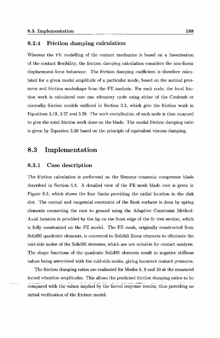
8.3. Implementation 168

8.2.4 Friction damping calculation

Whereas the FE modelling of the contact mechanics is based on a linearisation

of the contact flexibility, the friction damping calculation considers the non-linear

displacement-force behaviour. The friction damping coefficient is therefore calcu­

lated for a given modal amplitude of a particular mode, based on the normal pres­

sures and friction modeshape from the FE analysis. For each node, the local fric­

tion work is calculated over one vibratory cycle using either of the Coulomb or

microslip friction models outlined in Section 3.3, which give the friction work in

Equations 3.19, 3.27 and 3.39. The work contribution of each node is then summed

to give the total friction work done on the blade. The modal friction damping ratio

is given by Equation 3.20 based on the principle of equivalent viscous damping.

8.3 Implementation

8.3.1 Case description

The friction calculation is performed on the Siemens transonic compressor blade

described in Section 5.3. A detailed view of the FE mesh blade root is given in

Figure 8.2, which shows the four flanks providing the radial location in the disk

slot. The normal and tangential constraint of the flank surfaces is done by spring

elements connecting the root to ground using the Adaptive Constraint Method.

Axial location is provided by the lip on the front edge of the fir tree section, which

is fully constrained on the FE model. The FE mesh, originally constructed from

Solid95 quadratic elements, is converted to Solid45 linear elements to eliminate the

mid-side nodes of the Solid95 elements, which are not suitable for contact analysis.

The shape functions of the quadratic Solid95 elements result in negative stiffness

values being associated with the mid-side nodes, giving incorrect contact pressures.

The friction damping ratios are evaluated for Modes 8, 9 and 10 at the measured

forced vibration amplitudes. This allows the predicted friction damping ratios to be •--·- c,:, ""._'_!._, __ - - • ·:;:_, ----•7 - .....,;:_~ ---~·.o.:__ -~- ~·--J-. ,:__._:;, • ·--· -~~--· -·~ - "'___!~--::= : - - ••

compared with the values implied by the forced response results, thus providing an

initial verification of the friction model.

8.3. Implementation 169

8.3.2 Calculation of contact stiffness

The values of normal and tangential contact stiffness are derived from the microslip

friction model reported by Olofsson [130]. Two approaches to implementing the

Adaptive Constraint Method are presented, which represent the friction behaviour

in terms of the Coulomb and microslip models.

Coulomb friction analysis

The Coulomb friction model adopts constant values of normal and tangential spring

stiffness to represent the average contact properties over the whole contact area.

This approach demonstrates how the contact stiffness parameters can be be derived

either from experimental data or from a simple empirical or semi-analytical model.

The average contact pressure of the Siemens blade is calculated from the blade

centrifugal reaction load and the estimated contact area to give an estimated normal

contact pressure of Pn = 160M Pa. The tangential stiffness has been derived from

experimental data by Olofsson [130] and is obtained from the displacement-friction

load graph in Figure 9 of Olofsson [130]. This graph is based on the model described

in Section 3.3.2 and refers to stainless steel on stainless steel at a normal pressure of

125M Pa with contact parameters of C = 1.0 x 1010 contactsjm2 jm, R = lO.OJ.Lm

and J.L = 0.122. These values represent contact properties typical of unlubricated

engineering surfaces, and the case corresponds well with the conditions of the blade

root interface in terms of pressure and materials. Figure 8.5 shows how the tangential

stiffness is calculated from the graph of Olofsson. The stiffness is taken as the

gradient of the graph for the initial linear part of the microslip curve, giving a

tangential stiffness of 2.09 x 1012Njm3 •

Normal stiffness is taken as a factor of the tangential stiffness. It is discussed in

the friction literature that the ratio of normal to tangential stiffness is commonly

around 100 for machined metal surfaces. A value of }f,- = 100 is therefore used to t

define the normal stiffness.

, - ~- ~- ~-~ The· influence· ofthe~contact~parameters -on~the Elastic Coulomb damping~pre-- -~ -

dictions is investigated by repeating the calculations using a range of values in a

parametric study. The calculations are repeated with the following variations:

8.3. Implementation 170

P.' Contact stiffness (constant }if) P; = 2.09 x 1011 N/m3 , 2.09 x 1013N/m3

t

P.' Normal contact stiffness }it = 10, 1000 t

Friction coefficient jJ, = 0.2

The influence of the vibration amplitude on the predicted damping is also investi­

gated by repeating the Elastic Coulomb calculation at a range of modal amplitudes.

Microslip friction analysis

The microslip analysis uses the semi-analytical solution of Olofsson [130], to deter­

mine the normal and tangential contact stiffness as functions of normal pressure,

thus removing the assumption of constant stiffness properties made in the Coulomb

analysis. The microslip model uses the same parameters used to produce the graph

used in the above Coulomb friction approach, corresponding to Figure 9 of Olofsson.

A summary of the microslip parameters is given as

Surface contact parameter C = 1.0 x 1010

Spherical asperity radius R = 10JJ,m

Friction coefficient jJ, = 0.122

Young's modulus of elasticity E = 210GPa

Shear modulus G = 81G Pa

Poisson's ratio v = 0.3

The initial static analysis is performed using an average normal contact stiffness

in an identical manner to the Coulomb approach discussed previously. The stiffness

of each normal contact spring element in compression is then calculated at each

subsequent step, given by

(8.1)

Here, z is the normal deflection of the surface node, given by Equation 3.32, under

the-tesulting""notmal pressure, P.:t; and A0 is the effective nodal 'area of the -sur::

face node calculated by ANSYS. The stiffness values of the compressive springs are

updated and the tensile springs are deactivated before the static solution is repeated.

8.4. Results 171

Once the static analysis has reached convergence, the tangential stiffness proper­

ties are calculated for use in the modal analysis. The tangential stiffness is calculated

for each point in contact using the static normal pressure. Due to the non-linear

variation of friction force with tangential displacement, an equivalent linear stiffness

is derived for each active contact node. As shown in Figure 3.16, the equivalent

tangential stiffness is calculated at a defined position along the microslip curve. The

equivalent tangential stiffness is therefore given by the expression

(8.2)

where F1 is the microslip friction force given by Equation 3.34 at the specified

tangential displacement, x. The tangential displacement is specified as a fraction

of the of the slip displacement, xlim, which is given by Equation 3.35. A value of

xl~m = 0.5 is used as the datum value in the following friction calculations. In a

second analysis, the values of xl~m are varied for the Mode 8 calculation to assess

the influence on the predicted friction.

8.4 Results

8.4.1 Implied friction damping from forced response analy-.

SIS

In Section 5.3.2, the expected friction damping ratios of the three modes were calcu­

lated by subtracting the predicted aerodynamic damping from the measured system

damping. The expected friction damping ratios are listed in Table 5.7, showing

a value of 0.24% for Mode 8, whilst Modes 9 and 10 provide little or no friction

damping. This expected behaviour is characterised by the mode shape plots in Fig­

ure 5.13, where a significant level of root motion can be seen for Mode 8, whereas

the root motion of Modes 9 and 10 is much lower.

8.4. Results 172

8.4.2 Coulomb friction results

Static results

The convergence of the static contact analysis was reached in four steps, yielding the

compressive contact pressures for the contact nodes identified as active. Figure 8.6

plots the nodal reaction loads of each ANSYS static solution at each of the four

steps in the solution. The x-axis on each graph represents the node number of

each contact node, the ordering of which is arbitrary. The y-axis represents the

contact pressures, with negative values being compressive. It can be seen that the

normal stiffness for nodes in tensile contact are deactivated at the end of each step,

thus changing the distribution of the contact loads, and causing a small amount of

oscillation in the overall solution. Starting with normal stiffness applied to all 430

nodes around the root flanks, the number of active nodes at the end of the static

analysis is reduced to 204. The static contact analysis was repeated from a different

starting point, with only the nodes on the upper surfaces of the root flanks being

activated. The second analysis produced an identical end result, demonstrating that

the convergence is independent of starting point.

Modal result

Tangential spring stiffness is then applied to the springs of the active contact nodes

for the modal analysis. The resulting first 15 natural frequencies of the modal analy­

sis are plotted in Figure 8.7, together with the frequencies of the fully-constrained

root model used to provide the aerofoil modes in the forced response calculation.

The results of an additional analysis are included, where the modal analysis is done

without tangential stiffness to demonstrate the behaviour of freely-sliding contact.

Figure 8.8 compares the mode shape contours of three models. The comparison of

the elastic contact model with the original fixed root model shows that the natural

frequencies of the high-order modes vary a small amount with the change in root

constraints. However, the frequencies of the freely-sliding root model show signifi-

~--~'~"~'-- ~·-- c~nt -cfiffe~eil~es. The larg~st difference is the ·apparent addition of~ new lOth -mo,de,

characterised by the longitudinal vibration of the root along the slot due to the lack

8.4. Results 173

Modal Expected Rigid Coulomb Elastic Coulomb Mode Amplitude (jric (jric (jric

8 5.519 x 10-7 0.24% 22% 0.0027%

9 5.70 x 10-7 0.03% 5.9% 0.0000%

10 1.713 x 10-7 nil 40% 0.0001%

Table 8.1: Rigid and Elastic Coulomb friction damping predictions

of tangential constraint at the flank surfaces. This high level of mode shape sensi­

tivity demonstrates the importance of modelling the root contact mechanics with

the greatest possible accuracy.

The tangential displacement amplitudes at the contact surfaces for the three

modes at the forced response solution modal amplitudes are shown in Figure 8.9.

Here, it can be seen that the contact motion of Mode 8 is an order of magnitude

higher than Modes 9 and 10, agreeing well with the expected behaviour.

Friction calculation

The friction damping ratio of each mode is calculated using the Rigid Coulomb and

Elastic Coulomb models, based on 11 = 0.122, ~ = 100 and Pf = 2.09 x 1012.

t

The actual tangential displacements of each mode are gained from the product of

the contact surface mode shape and the modal amplitude of the forced response

solution. A summary of the friction results is given in Table 8.1, where the Rigid

and Elastic calculations can be seen to give remarkably different predictions. The

Rigid coulomb model predicts unrealistically high damping - especially for Mode

10, where a 40% damping ratio is predicted instead of the expected 0%. Conversely,

the Elastic Coulomb model predicts virtually no damping for all three modes.

Figure 8.10 shows the tangential displacement of each active friction contact

node, normalised to the elastic limit of the Elastic Coulomb model. Here, it can be

seen that only two nodes of a possible 204 active nodes achieve slip in the elastic

calculation.--. The Elastic- Coulomb dampingeoequation-{Equation 3;-281- states·- that

damping work can only be done by nodes in slip, therefore neglecting the contri­

butions from the 99% of active contact nodes that remain within the elastic limit.

8.4. Results 174

However, it is observed in practical applications that contact regions that do not

achieve gross sliding still contribute to friction damping due to microslip. It is

therefore apparent that the root contact displacements are generally too small to be

effectively modelled using the Elastic Coulomb approach.

The rigid model takes the opposite extreme by assuming that the all the tangen­

tial motion from every active node provides the maximum contribution to damping

for a given friction damping ratio. This approach vastly overestimates the contri­

butions from the regions with small-scale displacements, which make up the bulk of

the contact surfaces.

The behaviour of the Coulomb models for small displacements was illustrated

previously in Figures 3.5 and 3.9 for a simple 1 DoF case. Figure 3.5 shows that

very high damping ratios are predicted by the Rigid Coulomb model for very small

displacements. Whilst the Rigid Coulomb work increases linearly with displacement

amplitude, Equation 3.20 dictates that the damping ratio increases inversely propor­

tionally with the square of displacement amplitude. For very small displacements,

the squared term in the denominator dominates and the damping ratio becomes

very large, as seen in the case above. For the Elastic calculation, Figure 3.9 shows

that the damping work, and hence damping ratio is zero for displacements within

the elastic limit. Since 99% of the nodes in the above elastic calculation remain

within the elastic limit, the resulting damping ratio is very small.

Sensitivity to contact parameters

A parametric study was performed in order to investigate the sensitivity of the

friction predictions to the input friction contact parameters. The variation in the

predicted modal damping ratios with the contact stiffness is given in Table 8.2,

where the ratio of normal-tangential contact stiffness is held constant. Whilst the

friction is underpredicted, it can be seen that the stiffer contact stiffness gives higher

damping values. The higher tangential stiffness results in a reduced elastic limit,

allowing more nodes to achieve slip ~~dcontribute,to dampii1g:

Table 8.3 shows the variation of predicted damping with normal stiffness, which

is specified by varying the normal-tangential stiffness ratio, ~, for a constant P:. t

8.4. Results 175

Mode Expected (mech Predicted (mech

No. P! = 2.09 X 1011 P! = 2.09 X 1012 P! = 2.09 X 1013

8 0.24% 0% 0.0027% 0.0082%

9 0.03% 0% 0% 0%

10 0% 0% 0.0001% 0.050%

Table 8.2: Variation of predicted Elastic Coulomb friction damping with contact

stiffness

Mode Expected (mech Predicted (mech

No. .!:4- = 10 p ~ = 100 Pf .!:4- = 1000 p

8 0.24% 0.037% 0.0027% 0%

9 0.03% 0% 0% 0%

10 0% 0.02% 0.0001% 0%

Table 8.3: Variation of predicted Elastic Coulomb friction damping with normal

contact stiffness

This shows that the damping is slightly increased with reduced normal stiffness.

This is caused by a more uniform distribution of normal pressure over the contact

surfaces due to the higher contact flexibility. The increased pressure acting on the

lightly loaded nodes brings more nodes into slip by reducing the elastic limits.

The dependence on friction coefficient is shown in Table 8.4, where the calculation

is repeated using a value of J.t = 0.2. The increase in J.t allows a higher tangential

force to be sustained elastically, causing the elastic limit to be increased above

the displacements of all nodes. The elimination of all nodes in slip results in zero

damping.

The graph in Figure 8.11 shows the variation in damping ratio with modal am­

plitude for Mode 8 as the response amplitude is increased from zero to an order of

magnitude above the forced response amplitude. Marked on the graph are a series of

vertical lines,- whieh repi'esent the transition- point when an individual contact node

changes from stick to slip. These slip transition markers can be compared with the

normalised node displacements shown in Figure 8.10. At the forced response am-

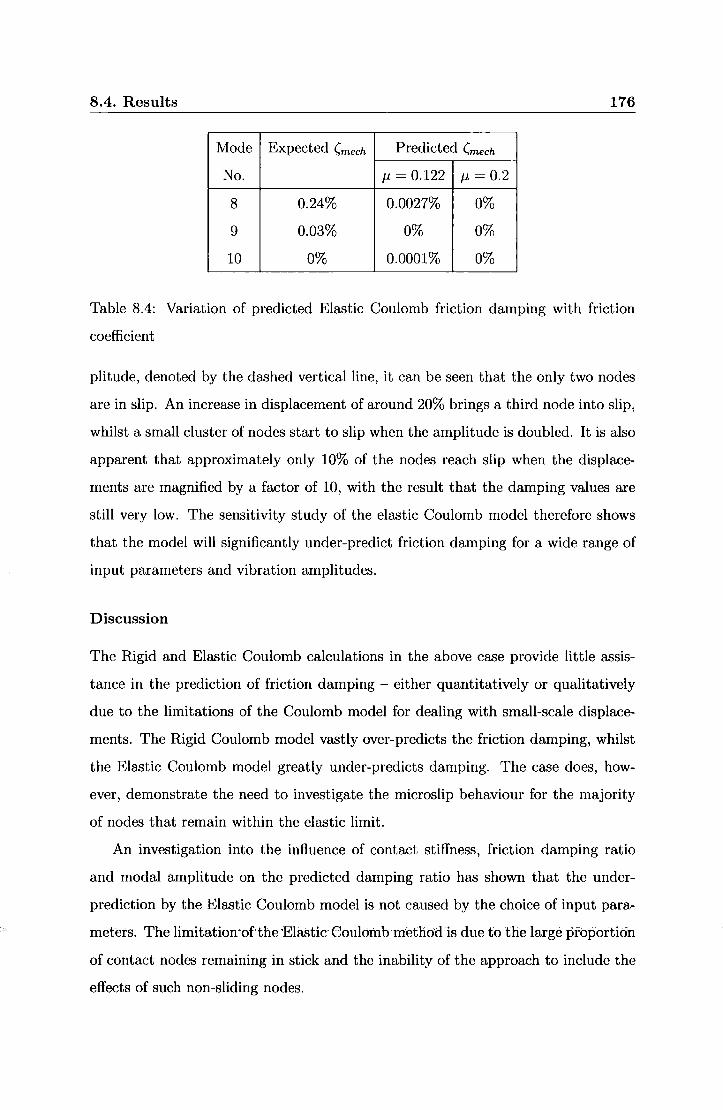
8.4. Results 176

Mode Expected (mech Predicted (mech

No. J-l = 0.122 J-l = 0.2

8 0.24% 0.0027% 0%

9 0.03% 0% 0%

10 0% 0.0001% 0%

Table 8.4: Variation of predicted Elastic Coulomb friction damping with friction

coefficient

plitude, denoted by the dashed vertical line, it can be seen that the only two nodes

are in slip. An increase in displacement of around 20% brings a third node into slip,

whilst a small cluster of nodes start to slip when the amplitude is doubled. It is also

apparent that approximately only 10% of the nodes reach slip when the displace­

ments are magnified by a factor of 10, with the result that the damping values are

still very low. The sensitivity study of the elastic Coulomb model therefore shows

that the model will significantly under-predict friction damping for a wide range of

input parameters and vibration amplitudes.

Discussion

The Rigid and Elastic Coulomb calculations in the above case provide little assis­

tance in the prediction of friction damping - either quantitatively or qualitatively

due to the limitations of the Coulomb model for dealing with small-scale displace­

ments. The Rigid Coulomb model vastly over-predicts the friction damping, whilst

the Elastic Coulomb model greatly under-predicts damping. The case does, how­

ever, demonstrate the need to investigate the microslip behaviour for the majority

of nodes that remain within the elastic limit.

An investigation into the influence of contact stiffness, friction damping ratio

and modal amplitude on the predicted damping ratio has shown that the under­

prediction by the Elastic Coulomb model is not caused by the choice of input para­

meters. The limitatioil~ofthe 'Elastic· Coulomb method is due to the large proportion

of contact nodes remaining in stick and the inability of the approach to include the

effects of such non-sliding nodes.

8.4. Results 177

Modal Expected Microslip (J-L = 0.122) Microslip (J-L = 0.2) Mode Amplitude (Jric (Jric (Jric

8 5.519 X 10-7 0.24% 0.11% 0.066%

9 5.70 X 10-7 0.03% 0% 0%

10 1.713 X 10-7 0% 0.01% 0.007%

Table 8.5: Rigid and Elastic Coulomb friction damping predictions

8.4.3 Microslip friction analysis

Results

The microslip model is verified by reproducing the force-displacement curve given

in Figure 9 of Olofsson [130], using the microslip parameters outlined above. Fig­

ure 8.12 shows a superposition of the original graph of Olofsson with the solution

reproduced using a spreadsheet. The excellent agreement between the analytical

solution of the microslip model with the original verifies that the calculation is done

correctly.

The resulting microslip damping predictions for the three modes using the datum

values outlined above in Section 8.3.2 are given in Table 8.5. It can be seen that the

microslip calculation agrees fairly well with the expected friction damping, where

only Mode 8 provides a significant amount of damping. Whilst the Mode 8 damping

ratio is under-predicted by 50%, this result captures the dependance of friction on

modeshape very well.

Sensitivity to input parameters

Included in Table 8.5 is the predicted damping ratios calculated using a different

friction coefficient of J-t = 0.2. Here, it can be seen that an increase in friction

coefficient reduces the damping ratio, whilst the trend of mode shape dependence

is maintained. Equation 3.35 states that the slip limit is proportional to friction

coefficient, giving an increased slip limit with ~n ~~c~ease in friction coefficient.

For a given displacement, the contact motion will be reduced in relation to the

microslip curve, giving less damping. Conversely, the increased slip limit gives a

8.4. Results 178

reduced effective tangential contact stiffness, resulting in an increased amount of

contact motion in the modes. The overall effect is highly non-linear, as shown by

the damping ratio-displacement curve in Figure 3.15. The result in this case is

reduced damping with increased friction coefficient.

A major simplification in the microslip approach is the assumption that the

effective tangential stiffness does not vary with the tangential displacement. The

approximation of the tangential stiffness of each node in the above calculations is

done using the microslip friction force at half the slip displacement. The sensitivity of

damping predictions to the choice of position along the microslip curve is assessed by

repeating the Mode 8 calculation using a range of positions. The resulting damping

ratios plotted in Figure 8.13 shows a reasonable variation in damping due to the

change in effective tangential stiffness. Calculating the tangential stiffness at very

small displacements gives the highest stiffness and lowest damping ratios, whereas

calculating the stiffness at the slip limit results in lower stiffness and higher damping.

The variation of predicted microslip damping with blade vibration levels is as­

sessed by repeating the Mode 8 calculation at a range of modal amplitudes above

and below the forced response solution. Figure 8.14 shows an almost linear increase

of damping ratio with an increase in response, where all nodes contribute to damp­

ing before they reach gross slip, preventing the sudden changes seen in the Elastic

Coulomb results presented earlier. The damping behaviour of this multi-DoF prob­

lem can be compared to the graph of the single-DoF system provided in Figure 3.15.

Both microslip systems are seen to provide an almost linear increase of damping ra­

tio with response amplitude for the very low contact displacements seen at the blade

root.

Discussion

The microslip damping predictions agree very well with the expected values for

all three modes. The dependence on mode shape is well-captured, with Mode 8

providing a significant amount of damping and Modes 9 and 10 providing almost no ·---·~··__:· __ ;.._,_:-=:o""'·:.._:._""·ro,: .7;:..•:.,,;:_.-•· " -·"··· _, ,:_- _;_· <-'·-~0 -- .:.-; .• •• •• -~--~" •• • -~--~~ ;',,.,_- • -~ -~ o'.

damping. The Mode 8 damping was predicted within around 50% of the expected

value using published input parameters that have been verified for the same materials

8.5. Conclusions 179

under similar contact conditions.

The friction behaviour does not show a high sensitivity to the input parameters,

displaying a smooth variation in damping as the parameters are varied. Similarly,

the method of calculating the effective tangential stiffness does not cause a large

variation in results.

The microslip calculation predicts an almost linear increase of damping ratio

with modal amplitude around the range of the forced response solution. This is

due to the fact that the large majority of nodes in compressive contact are subject

to very small tangential displacements that are much lower than the elastic limits.

The near-linear behaviour for small displacements is also seen in the solution of a

simple single-DoF microslip system, shown in Figure 3.15. However, experimental

measurements of mechanical damping of fixed root blades can often suggest that

damping remains fairly constant over typical ranges of blade vibration. Whereas the

predicted blade microslip damping shows a similar linear characteristic to a simple

1-D brick-type object undergoing pure microslip, the comparison with experimental

behaviour suggests that either a) more complex physical mechanisms are present;

or b) the linearisation process is not capturing some important non-linear effects.

8.5 Conclusions

A new Adaptive Constraint Method for modelling blade root friction has been de­

veloped and successfully implemented for an industrial compressor blade. Based on

an advanced microslip model, the friction predictions agree with the damping values

derived from test data.

The new method meets many of the requirements for use in industry. The

frequency-domain solution allows the modal friction damping ratios to be calculated

based on a single FE analysis with high computing efficiency. User interaction is

very low, with a high level of automation provided by a series of ANSYS macros to

modify the existing FE model and perform the analysis. The only area of significant

user effort is in the identification of nodes on the root surface, resulting in an overall

effort that is much less demanding than a standard time-accurate ANSYS contact

8.5. Conclusions 180

analysis.

It has been demonstrated that the Rigid and Elastic Coulomb friction models

are not suitable for the prediction of friction damping at the blade root due to their

inability to deal with the very low displacements. The Elastic Coulomb analysis of

Mode 8, shows that only 2 nodes out of the 204 nodes in contact actually reach slip,

with the result that the damping contributions of the remaining 99% of the contact

nodes are neglected and the friction damping is vastly under-predicted. Conversely,

the Rigid model greatly over-predicts damping by assuming that the entire friction

surface achieves gross sliding.

Whilst the friction behaviour predicted by the Coulomb approaches has been

shown to be sensitive to the model parameters, the microslip model is much more

robust and does not show any sudden changes with contact parameters or response

amplitude. An additional observation is the linear increase of damping ratio with

response amplitude predicted by the microslip model. An area of question is the

method of calculating the effective tangential stiffness using the microslip model,

where stiffness is calculated using a fixed point on the microslip curve. A variation

in the assumed displacement produces a change in damping, hence an area for

improvement could be to calculate the effective tangential stiffness as a function of

actual displacement.

8.6. Figures

8.6 Figures

I

frequency, mode shape

I ...

CFD Damping Calculation

I aerodynamic

ADAPTIVE CONSTRAINT METHOD damping

-----------1 FE Model I. J Friction Model 1 I

------------contact sttffnesses,

surface mode shape modal am p,

friction damping

181

FE Modal Analysis

~ FE-CFD I Interpolation

I ...

CFD Forcing Calculation

I

l aerodynamic forcing

Forced Response Analysis

Figure 8.1: Application of friction calculation into decoupled forced response system

8.6. Figures 182

Figure 8.2: Friction contact nodes on surfaces of root flanks

Figure 8.3: Spring representation of 3-D contact stiffness at each contact node

8.6. Figures

FE Model with Contact Springs

Modal Analysis

contact surface mode shape

Friction Damping 14----t Modal Amplitude Calculation

Figure 8.4: Adaptive Constraint Method of FE friction modelling

2000

z 1500

~ .9 -;;; c 1000 .g

.\,! .. u..

500

7.5

1922 I ---------T--:... -~""'""::~~~,.....,.,_ I //.

I/. /.

oL---~----~----L---~----~----~--_.--~ 0 5 10 15

Displacement ( >' m)

Figure 8.5: Derivation of tangential stiffness from microslip curve

183

8.6. Figures

'C

~ c 0

~ e iii 'C 0 c

184

Figure 8.6: Nodal pressures after each static solution, showing convergence of static

contact analysis

16000

14000

12000 N" ~ 10000 >-0

8000 c: Gl :>

~ 6000 u_

4000

2000

0

Results of modal analysis

DFixed root

• Elastic root (ACM)

Freely sliding root

2 3 4 5 6 7 8 9 10 11 12 13 14 15

Mode

Figure 8. 7: Blade modal frequencies using Coulomb approach

8.6. Figures

Root constraint method · · · · · · ··· · freely sliding ----·elastic

rigid

ModeS Mode9

185

Mode 10

Figure 8.8: Comparison of mode shapes for various methods of root constraint

600 !Jm 441Jm

ModeS Mode9 Mode 10

Figure 8.9: Tangential contact displacements at modal forced response solutions

8.6. Figures 186

1.40 ~--------------------------------------------------~

c 1.20 +------------------------------f Q)

E Q)

SLIP

~ 1 .oo ~~~~~~~~~~~~~~~~~~~~~~~~~~~~

a. en '6

STICK

Q) 0 .80 +---------------------------~ '0 0 c

al 0.60 +----------------------------­.!!! (ij E 0 0.40 +---------------------------c

I a. U5 0.20 +--------------------------

0.00 _t_ ______ _ ___________ ...

Ranked Nodes

Figure 8.10: Mode 8 tangential contact displacements normalised to elastic limit

0.030

- 0.025 eft -;- 0.020 iii '; 0.015 c

·~ 0.010 \U

Q 0.005

0.000

Solution Amplitude

{ !---"

I

DAMPING RATIO Vs. DISPLACEMENT (with slip transition markers)

I ----I

v I

O.OOE+OO 1.00E-06 2.00E-06 3.00E-06 4.00E-06 5.00E-06 6.00E-06 ?.OOE-06

Modal Amp

Figure 8.11: Variation of damping ratio with response amplitude for mode 8, showing

individual node stick-slip transit ion points

8.6. Figures

-- Microslip (Moffatt) - - Microslip (Oiofsson) .......-vv Experiment (Oiofsson)

0~--~~--~-----L----~----L---~~--~--0 5 10

Displacement (~ m) 15

187

Figure 8.12: Comparison of microslip calculation with original calculation of Olofs­

son, 1995

0.25

~ 0.2 0 ~ 0.15 .... Cl

·8. 0.1 E ~ 0.05

0 0.25 0.5 0.75

Position along microslip curve (X/XIim)

Figure 8.13: Variation of predicted microslip friction damping with position of ef­

fective-stiffness calculation for Mode 8

8.6. Figures

0.15

2 0.1 <1S ... 0) c ·a. 0.05 E <1S a

0~---,--------,-----,------,

O.OE+OO 2.0E-Q7 4.0E-07 6.0E-07 S.OE-07

Modal amplitude

188

Figure 8.14: Variation of predicted damping with response amplitude for Mode 8

Chapter 9

Conclusions and

Recommendations

9.1 Conclusions

The objective of this project was to develop an efficient and accurate aeromechanical

analysis tool capable of providing reliable resonant forced response predictions for

turbomachinery blade designers under the commercial restraints of solution times

and computing resources. Both decoupled and fully-coupled approaches for the mod­

elling of flow-structure interaction have been developed and the capabilities of such

methods to capture important coupling effects have been evaluated. In addition, a

method of predicting the friction damping of fir-tree type blade root attachments

has been developed, leading to an evaluation of the mode shape dependence and the

importance of microslip behaviour.

9.1.1 Decoupled forced response system

The decoupled method represents an open loop system, requiring only a single execu­

tion of the flow and structural equations. Blade mode shapes and natural frequencies

are assumed to remain unchanged by aerodynamic loads due to the high relative

densfty ana' stiffness of turbomachlnery blades. The -FE- modal analysis is evaluated

independently to the fluid calculations, where blade mode shapes are accurately

189

9.1. Conclusions 190

translated onto the CFD mesh to enable a forced response solution in modal space

based on the CFD mesh.

A method for interpolating the modeshapes from the FE to CFD mesh has been

produced, based on 2D linear interpolation over the blade surface. The capabilities

of the method are demonstrated with an industrial case, where difficulties of mesh

alignment, non-coincident mesh surfaces, low mesh resolution and high mode shape

gradients are overcome and excellent accuracy of mode shape interpolation is seen.

Flow is modelled by the nonlinear harmonic method, solving the unsteady Navier­

Stokes equations in the frequency-domain using a single-passage approach, whilst

maintaining the ability to include important non-linear effects. With single degree­

of-freedom structural modelling based on modal reduction, the system can predict

resonant vibration levels 30-100 times faster than direct time-domain schemes.

Fluid-structure interaction is modelled on a linear basis, assuming that aerody­

namic damping loads increase linearly with vibration amplitude. This allows the

calculation of aerodynamic forcing and damping to be done separately from one­

another, and independently to the forced response solution.

The decoupled forced response solution is calculated using conventional modal

reduction theory, reducing the structural FE model to a single degree-of~freedom

modal equation. In addition, a new energy method provides an alternative to the

solution of the modal equation, which solves the response directly on the CFD mesh

without the knowledge of original modeshape scaling. Both methods are shown to

give identical results.

9.1.2 Verification Cases

A detailed demonstration of the forced response system and an initial verification

of the individual system components has been done using a case study of the NASA

Rotor 67 transonic aero engine fan. The resonant excitation of three low order

modes and one high order mode is given by hypothetical inlet distortions, to pro­

vide a realistic test case that is typical of inlet distortion and bladerow interaction

problems.

Validation of the forced response system has been done against the Siemens 3-

9.1. Conclusions 191

stage transonic industrial compressor, where predicted resonant strains and damp­

ing levels are compared with measured strain gauge data from a full-scale rotating

test. The vibration of three high-order modes of the last rotor stage is predicted,

with excitation caused by interference from the upstream stator wakes. The damp­

ing calculations have shown that aerodynamic damping is strongly influenced by

modeshape and a comparison with strain gauge data also indicates a strong corre­

lation between mechanical damping and modeshape. Predicted resonant strains for

the three crossing points compare reasonably well with strain gauge measurements,

demonstrating the ability of the method to predict resonant vibration levels. The

high efficiency of the unsteady multi-stage calculation also demonstrates the system

can be used routinely in the blade design process to tackle aeromechanical issues,

where the 3D unsteady viscous CFD analysis of the 3-stage compressor was achieved

in under a week on a single CPU.

9.1.3 Fully-coupled forced response systems

Two fluid-structure fully-coupled forced response methods have been developed with

the intention of increasing computational efficiency over the decoupled method by

combining the calculation of aerodynamic excitation and damping forces into a single

calculation. The modal equation is fully integrated into the flow solver and solved

either directly in the frequency domain or by time-marching using a hybrid approach.

The frequency-domain method simultaneously solves the fluid and modal equa­

tions by pseudo-time integration using the 4-stage Runge-Kutta scheme, where aero­

dynamic forcing and blade displacement amplitudes are exchanged at each step.

The hybrid approach solves the fluid equations in the frequency domain, but

marches the modal equation in time with periodic updating of the reconstructed

aerodynamic modal force. A Fourier transform of the continuous time trace of the

modal displacement is taken after each forcing period to give the response modal

amplitude. The resulting blade displacement amplitudes are then fed back into the

< fluid, equations to close theJeedbackJoop. Both,Jully-coupled systems are shown

produce identical results, serving a cross-checking purpose.

9.1. Conclusions 192

9.1.4 Fluid-structure coupling effects

An investigation into the characteristics of decoupled and fully-coupled methods

was undertaken using the four modes of the NASA Rotor 67 transonic fan case. It

was shown that decoupled systems can accurately predict resonant vibration ampli­

tudes from a single calculation at the blade natural frequency, whilst fully-coupled

forced response solutions are subject to a shift in resonant frequency, thus requiring

multiple solutions. A novel closed-loop resonance tracking algorithm was incorpo­

rated into the coupled solution to adjust the solution frequency and obtain the peak

vibration amplitude at the new resonant condition. Due to the need for multiple

solutions, the computational efficiency of the coupled solution showed no gain over

the decoupled method. In contrast, the decoupled method is shown to be insensi­

tive to frequency shift, maintaining resonance at the blade natural frequency and

capturing the resonant peak with one solution.

A study into the fluid-structural coupling effect identified the source of the fre­

quency shift in the coupled solution to be due to the added mass effect of the

vibration-induced aerodynamic damping forces. A single coupled solution at any

frequency can not be used to predict resonance; hence coupled methods must rely

on multiple solutions to find the resonant peak. The need for resonance tracking

with coupled methods is especially important for high-order modes, which are often

associated with low mechanical damping and strong fluid-structure coupling effects.

The decoupled method is identified as the preferred approach to bladerow inter­

action problems due to the ability to accurately predict the resonant peak with high

efficiency from a single solution.

9.1.5 Friction Modelling

A new Adaptive Constraint Method for predicting blade root friction has been de­

veloped and implemented for the Siemens industrial compressor blade. The model

is based entirely in the frequency domain using a FE modal approach to maximise

coiiiputing efficiency and maintain high c6nipatib1lity with the existing forced re­

sponse system.

9.1. Conclusions 193

Contact mechanics are represented using traditional Coulomb friction models and

an advanced semi-analytical microslip model. Normal and tangential contact loads

are linearised on an FE blade model by a series of spring elements. Non-linearity

in the contact mechanics is incorporated by performing the FE static analysis in

an iterative manner, where the stiffness values are updated at each step. A modal

analysis is performed to provide the mode shape over the contact surfaces, allowing

the friction damping calculation to be done separately.

The Coulomb and microslip contact behaviour is derived from a published mi­

croslip model, where input parameters were fitted to test data for similar contact

conditions. The predicted damping ratios are compared with the mechanical damp­

ing values derived from test data.

It was found that the damping predictions of the Rigid and Elastic Coulomb

friction models were very inaccurate due to their inability to deal with the very low

displacements involved. Neither Coulomb approach predicted the trend with mode

shape, with the Rigid model vastly over-predicting damping and the Elastic model

predicting almost no damping. The under-prediction of the Elastic approach is due

to the very small proportion of contact nodes reaching slip, where the contributions

from 99% of all contact nodes are neglected. The very high prediction by the Rigid

model is due to the assumption that the entire contact surface achieves gross slip.

The Coulomb predictions are very sensitive to variations in contact parameters due

to the small proportion of nodes reaching slip, where the contribution from a single

node reaching slip causes a sudden change in the overall behaviour.

The microslip damping predictions showed good agreement with the expected

behaviour, where the dependence on mode shape was captured well and the damping

levels were predicted within 50%. The microslip model is well suited to small dis­

placement applications where very little gross slip is achieved. The method includes

the contribution of each individual contact node, based on the knowledge that a de­

gree of damping is always encountered before gross slip takes place. The microslip

model is much more robust than the Coulomb models and does not produce sudden

changes in damping with variations in contact parameters or vibration amplitude.

The Adaptive Constraint Method has achieved the original objective of providing

9.2. Recommendations for Future Research 194

a qualitative prediction of friction damping for the three modes of the Siemens

compressor case, together with a quantitative indication of the damping levels. The

scheme meets many of the requirements for routine use in an industrial environment,

allowing the efficient prediction of all modes with a single analysis. User interaction

is low due to the high level of automation using ANSYS macros, greatly reducing

the manual processing time needed for conventional time-domain solutions.

9.2 Recommendations for Future Research

9.2.1 Forced response system

Further Evaluation

It is recognised that further evaluation of the forced response system using realistic

test cases is necessary for full validation of the methodology. Whilst the aerodynamic

solver has been validated for a number of academic and industrial cases, further

assessment of the complete forced response system against detailed strain gauge

measurements in full-scale rotating engine tests would be beneficial.

Modal Interaction

Further research could look at the effects of increasing the number modes used in

the forced vibration analysis. The current system uses only a single flow harmonic

applied to a single mode for the crossing point in question, based on the assumption

that all frequencies outside resonance have a negligible effect on vibration ampli­

tudes. This assumption is generally adequate for cases where the modal frequencies

are placed sufficiently far from one another, such that the effects of modal coupling

can be ignored. It is possible that a forced response approach that accounts for

modal coupling could provide greater accuracy in predictions for modes 8 and 9 of

the Siemens compressor case study given in Section 5.3.

For cases where two modes are placed close to a resonant frequency, modal

coupling may have a significant effect on both the dynamics and forced response of

the system. The close proximity of two modes introduces a coupling effect, where

9.2. Recommendations for Future Research 195

the modal properties of the two individual modes begin to share characteristics as

they come closer in frequency. Consider a blade where the 2nd flap mode (F2 ) lies

close to the 1st torsion mode ( T1). The flap mode will display a degree of twist in

the tip and the torsion mode will contain an amount of F2 mode shape. A result

of this modal coupling is that the presence of the T1 mode shape in the F2 mode

causes the F2 mode to be influenced by any forcing distribution similar to the T1

modal force. Similarly, the T1 mode will be influenced by the F2 forcing. Therefore,

any blade motion caused by the the forced response in one mode will contribute to

the motion from the other mode, with the subsequent increase in modal strains.

It may be possible to provide a simple two-mode evaluation using the decoupled

method with a frequency sweep. For each of the two modes, the decoupled responses

are calculated individually at a single frequency, with a linear superposition of the

resulting modal displacements and strains. The process is repeated around the two

natural frequencies to find the peak responses. Using the coupled approach, the two

modal equations are solved simultaneously by the frequency-domain CFD solver,

subject to unsteady pressures calculated at the solution frequency.

9.2.2 Root Friction Modelling

Whilst the friction prediction method shows very promising results, the develop­

ment of the Adaptive Constraint Method is relatively immature and further work is

required to improve the methodology and provide further validation.

Full FE transient analysis

At this stage, it is important to have a benchmark friction prediction method ca­

pable of producing reliable results, thus providing a comparison for the results of

new methodologies. A suggestion for the benchmark method would be an ANSYS

transient analysis, where the friction forces are resolved in the time-domain and the

linearisation of contact loads is avoided. Such an approach would be useful for eval-

0 uating the general behaviour of the Adaptive Constraint Method in both Coulomb

and microslip applications for varying levels of displacement amplitudes. The pro­

cedure for Coulomb friction calculations is standardised and is well documented.

9.2. Recommendations for Future Research 196

The microslip model given by Olofsson [130] implemented in this work has previ­

ously been incorporated into ANSYS by the developers of the model, as discussed

by Sellgren and Olofsson [150]. This time-accurate microslip model integrated into

the FE solver would provide a good ground for further evaluation of the Adaptive

Constraint Method.

Simple test case

Preliminary test cases do not need to include the complexities of a blade fir-tree root

and simplified models may provide a useful insight into the underlying characteristics

of the methods. A good starting point may be the analysis of a flexible brick­

type structure of low mesh density on a rigid, flat friction surface. Subject to a

simple static loading condition, the friction damping can be calculated for a range of

conditions to isolate individual characteristics of the solution methods. For example

a variation in the tangential displacement amplitude or normal pressure distribution

will provide an evaluation of the limiting boundaries of the Coulomb and microslip

models. A simplified model will also allow the assessment of input parameters

against any published test data.

Linearisation of tangential stiffness

A possible area for future investigation is in the calculation of effective tangential

stiffness in the microslip analysis. The tangential stiffness remains fairly constant

from zero to around 50% of the gross slip limit. After this, the effective stiffness is

reduced as the surface starts to slip. In order to model the tangential stiffness with

the greatest possible fidelity within the linear framework could be to incorporate

an iterative modal analysis, to linearise the effective stiffness for a given modal

amplitude. The inclusion of the response modal amplitude in modal analysis would

therefore allow each tangential stiffness to be calculated as a function of absolute

displacement. The modification of the tangential stiffness will be incorporated in the

ana,Jy~is by performjng the modal analysis in an iterativ~ manqer in a silllilar ~ay _to

the static analysis. An area of concern with this method is the convergence stability

of the modal analysis due to the updating of the effective tangential stiffness. Whilst

9.2. Recommendations for Future Research 197

the normal stiffness is increased with increasing pressure (and normal deflection),

the effective tangential stiffness is reduced with displacement, as the force curve

levels off. The implications of this softening effect are currently unknown.

Bibliography

[1] Kielb, R.E. (1999), Forced Response Analysis- 1, Aeroelasticity in Axial Flow

Thrbomachines, Lecture Series 1999-05, von Karmen Institute for Fluid Dy­

namics, May 3-7, 1999.

[2] Fransson, T. (1999), Basic Introduction to Aeroelasticity, Aeroelasticity in

Axial Flow Thrbomachines, Lecture Series 1999-05, von Karmen Institute for

Fluid Dynamics, May 3-7, 1999.

[3] Wisler, D. C. (2003), Engineering What You Dont Necessarily Learn in School,

ASME paper GT2003-38761.

[4] Kielb, R.E. (1999), Aeroelastic Models, Aeroelasticity in Axial Flow TUrbo­

machines, Lecture Series 1999-05, von Karmen Institute for Fluid Dynamics,

May 3-7, 1999.

[5] Marshall, J.G. (1996), Prediction of Turbomachinery Aeroelasticity Effects Us­

ing A 3D Non-Linear Integrated Method, PhD Thesis, Imperial College of

Science Technology and Medicine, University of London, 1996.

[6] Fransson, T. (1999), Important Parameters, Aeroelasticity in Axial Flow Thr­

bomachines, Lecture Series 1999-05, von Karmen Institute for Fluid Dynamics,

May 3-7, 1999.

[7] Ewins, D.J. (1991), The Effect of Blade Mistuning on Vibration Response -

A Survey, IFToMM 4th International Conference on Rotordynamics, Prague,

Czechoslovakia, 1999.

198

Bibliography 199

[8] Bowden, F.P. and Tabor, D., 1974, An Introduction to Tribology, Heinemann

Educational.

[9] Kielb, R.E. and Imregun, M., (1999), Damping Characteristics, Aeroelasticity

in Axial Flow Turbomachines, Lecture Series 1999-05, von Karmen Institute

for Fluid Dynamics, May 3-7, 1999.

[10] MacCormack, R. W. (1969), The Effect Of Viscosity In Hypervelocity Impact

Cratering, AIAA Paper No. 69-0354, 1969.

[11] Jameson, A Et Al (1983), Numerical Solutions Of The Euler Equation By Fi­

nite Volume Method Using Runge-Kutta Time-Stepping Scheme, AIAA Jour­

nal, Vol 32, No. 1, pp46-53, 1983.

[12] Fransson, T. and Pandolfi, M. (1986), Numerical Investigation of Unsteady

Subsonic Compressible Flows Through an Oscillating Cascade, ASME Paper

86-GT-304, 1986.

[13] Gerolymos, G. A. (1988), Numerical Integration of the Blade-Blade Surface

Euler Equations in Vibrating Cascades AIAA Journal, Vol. 26, No.12, pp1483,

1988.

[14] He, L. (1990), An Euler Solutionfo Unsteady Flows Around Oscillating Blades,

Journal of Turbomachinery, Vol. 112, pp. 714, 1990.

[15] Giles, M.B. (1988), Calculation of Unsteady Wake/Rotor Interaction, AIAA

Journal of Propulsion, Vol. 4, No.4, pp.356, 1988.

[16] Namba, M. (1977), Three-Dimensional Analysis of Blade Force and Sound

Generation for an Annular Cascade in Distorted Flows, Journal of sound and

Vibration, Vol. 50, pp. 479-508, 1977.

[17] Chi, R.M. (1991), An Unsteady Lifting Surface Theory for Ducted Fan Blades,

ASME Paper 91-GT-131, 1991.

Bibliography 200

[18] Hall, K.C. and Lorence, C.B. (1992), Calculation of Three-Dimensional Un­

steady Flows in Turbomachinery Using the Lineazed Harmonic Euler Equa­

tions, ASME Paper, 92-GT-136, 1992.

[19] Gerolymos, G.A. (1992), Advances in the Numerical Integration of of the 3-D

Euler Equations in Vibrating Cascades, ASME Paper 92-GT-170, 1992.

[20] Marshall, J.G and Giles, M.B. (1997), Some Applications of a Time-Linearised

Euler Method to Flutter and Forced Response in Turbomachinery, Proceedings

of the 8th International Symposium on Unsteady Aerodynamics and Aeroelas­

ticity of Turbomachines, Stockholm, Sweden, 1997.

[21] He, L., Denton, J.D. (1994), Three-Dimensional Time-Marching Inviscid And

Viscous Solutions For Unsteady Flows Around Vibrating Blades, ASME Jour­

nal Of Turbomachinery, July 1994, Vol 116, pp469-475, 1994.

[22] Rai, M.M. (1987), Unsteady Three-Dimensional Navier-Stokes Simulations of

Turbine Rotor-Stator Interaction, AIAA-87-2058, 1987.

[23] Chen, J.P., Celestina, M.L. and Adamczyk, J.J. (1994), A New Procedure for

Simulating Unsteady Flows Through Turbomachinery Blade Pasasges, ASME

Paper 94-GT-151, 1994.

[24] Erdos, J. I. And Alzner, E. (1978), Computation Of Unsteady Transonic Flows

Through Rotating And Stationary Cascade, NASA Cr-2900, 1978.

[25] Rai, M.M. (1985, Navier-Stokes Simulations of Rotor-Stator Interaction Using

Patched and Overlaid Grids, AIAA Paper 85-1519, 1985.

[26] He, L. (1989), An Euler Solution For Unsteady Flows Around Oscillating

Blades, ASME Journal, Vol. 112, 1989.

[27] He, L. (1992), A Method of Simulating Unsteady Turbomachinery Flows with

Multiple Perturbations, AIAA Journal, Vol. 30, No. 12, 1992.

Bibliography 201

[28] Whitehead, D.S. (1960), Force and Moment Coefficients for Vibrating Aero­

foils in Cascades, Reports and Memoranda No. 3254, Aeronautical Research

Council, London, 1960.

[29] Whitehead, D.S. (1970), Vibration and Sound Generation in a Cascade of Flat

Plates in Subsonic Flow, A.R.C. R&M, No. 3876, 1970

[30] Namba, M. (1972), Lifting Surface Theory for a Rotating Subsonic or Tran­

sonic Bladerow, A.R.C. R&M, No. 3740, 1972.

[31] Verdon, J.M. and McCune, J.E. (1975), Unsteady Supersonic Cascade in Sub­

sonic Axial Flow, AIAA Journal, Vol. 13, No. 2, pp. 193-201, 1975.

[32] Whitehead, D.S. (1987), Classical Two-Dimensional Methods, AGARD Man­

ual on Aeroelasticity in Axial-Flow Thrbomachines, Unsteady Thrbomachin­

ery Aerodynamics, Vol. 1, AGARD-AG-298, 1987.

[33] Whitehead, D.S. (1982), The Calculation of Steady and Unsteady Transonic

Flow in Cascades, University of Cambridge, Department of Engineering Re­

port CUED/ A-Thrbo/TR118, 1982.

[34] Verdon, J.M. and Caspar, J.R. (1984), A Linearised Unsteady Aerodynamic

Analysis For Transonic Cascades, J. Fluid Mechanics, 149 pp 403-429, 1984.

[35] Hall, K.C. and Verdon, J.M. (1991), Gust Response Analysis for Cascades in

Non-Uniform Mean Flow, AIAA Journal, Vol. 29, No.9, pp. 1463-1471, 1991.

[36] Ni, R.H. (1974), Nonstationary Aerodynamics of Arbitrary Cascades in Com­

pressible Flow, PhD Thesis, Stevens Institute of Technology, June, 1974.

[37] Hall, K.C. and Crawley, E.F. (1989), Calculation of Unsteady flows in Turbo­

machinery Using the Linearised Euler Equations, AIAA Journal, Vol. 27, pp.

777-787, 1989.

--[38]-I:;indqiiist, D.R. and Giles, M.B. (1991), On the Validity of Linearised Euler

Equations With Shock Capturing, AIAA 91-1598-CP, 1991.

Bibliography 202

[39] Hall, K.C., Clark, W.S. and Lorence, C.B. (1994), A Linearised Euler Analysis

of Unsteady Transonic Flows in Turbomachinery, Journal of Turbomachinery,

Vol. 116, No. 3, July, pp477-488, 1994.

[40] Cizmas, P.G.A. and Hall, K.C. (1995), A Viscous-Inviscid Model of Unsteady

Small-Disturbance Flows in Cascades, AIAA Paper No. 95, pp. 2655, 1995.

[41] Holmes, D.C. Mitchell, B.E. and Lorence, C.B. (1997), Three-Dimensional

Linearised Navier-Stokes Equations for Flutter and Forced Response, Pro­

ceedings of the 8th International Symposium on Unsteady Aerodynamics and

Aeroelasticity of Turbomachines, Stockholm, Sweden, 1997.

[42] Clark, W.S. and Hall, K.C. 2000, A Time-Linearized Navier-Stokes Analysis

of Stall Flutter, ASME Journal of Turbomachinery, Vol. 122, pp. 467-4 76,

2000.

[43] Sbardella, L. and Imregun, M. (2001), Linearised Unsteady Viscous Turboma­

chinery Flows Using Hybrid Grids, ASME Journal of Turbomachinery, Vol.

123, July, pp. 568-582, 2001.

[44] Giles, M.B. (1992), An Approach for Multi-stage Calculations Incorporating

Unsteadiness, ASME 92-GT-282, 1992.

[45] He, L. (1996), Modelling Issues for Computation of Unsteady Turbomachinery

Flows, Unsteady Flows in Turbomachines VKI Lecture Series, March 1996.

[46] Hall, K.C., Thomas, J.P. and Clark, W.S. (2002), Computation of Unsteady

Nonlinear Flows in Cascades using a Harmonic Balance Technique, AIAA

Journal, Vol. 40, No, 5, pp. 477-886, 2002.

[47] Vasanthakumar, P. (2003), Three dimensional Frequency-domain Solution

Method for Unsteady Turbomachinery Flows, PhD Thesis, University of

Durham, 2003.

[48] Vasanthakumar, P., Chen, T. and He, L. (2000), Three-Dimensional Viscous

Computation of Blade Flutter and Forced Response using Nonlinear Harmonic

Bibliography 203

Approach, The 9th International Symposium on Unsteady Aerodynamics and

Aeroelasticity of Turbomachines, September 4-8 2000, Editors Ferrand, P. and

Aubert, S., Published by Presses Universitaires de Grenoble, 2000.

[49] Chen, T., Vasanthakumar, P. and He, L. (2001), Analysis of Unsteady

Bladerow Interaction Using Non-Linear Harmonic Approach, AIAA Journal

of Power and Propulsion, Vol. 17, No. 3, May 2001; also ASME Paper 2000-

GT-431, 2000.

[50] Ning, W., Li, Y.S. and Wells, R.G. (2003), Predicting Bladerow Interactions

Using a Multistage Time-Linearised Navier-Stokes Solver, Journal of Turbo­

machinery, Jan 2003, Vol. 125, Issue 1, pp. 25-32, 2003; ASME Paper 2002-

GT-30309, 2002.

[51] Ning, W., Moffatt, S., Li, Y., Wells, R.G. (2003), Blade Forced Response

Prediction for Industrial Gas Turbines, Part 2: Verification and Application,

ASME GT2003-38642, 2003.

[52] Campbell, W. (1924), The Protection of Steam Turbine Wheels from Axial

Vibration, Proceedings of the Cleveland Spring Meeting, ASME, May 1924.

[53] Bishop, R.E.D. and Johnson, D.C. (1960), Mechanics of Vibration, Cambridge

University Press, 1960.

[54] Ballhouse, W.F. and Goorjan, P.M. (1978), Computation of Unsteady Tran­

sonic Flows by the Indica[ Method, AIAA Journal Vol. 16, No. 2, pp. 117,

1978.

[55] Guyan, R.J. (1965), Reduction of Stiffness and Mass Matrices, AIAA Journal,

Vol. 3, No. 2, pp. 380, 1965.

[56] Chiang, H-W.D. and Kielb, R.E. (1992), An Analysis System for Blade Forced

Response, ASME Paper, 92-GT-172, 1992.

[57] Manwaring, S~R. ahd Kh~keng, K.E. (1997), Forced Response Vibrations of a

Low Pressure Turbine Due to Circumferential Temperature Distirtions, 8th

ISUAAAT Symposium, Stockholm, 1997.

Bibliography 204

[58] Schmitt, S., Nurnberger, D. and Carstens, V. (2003), Evaluation of the Prin­

ciple of Aerodynamic Superposition in Forced Response Calculations, lOth In­

ternational Symposium on Unsteady Aerodynamics and Aeroelasticity of Thr­

bomachines Symposium, Duke University, Durham, NC, USA, Sept 7-11 2003.

[59] Green, J.S. and Marshall, J.G. (1999), {it Forced Response Prediction Within

The Design Process, 3rd European Conference on Turbomachinery, London,

March 1999.

[60] Filsinger, D., Szwedowicz, J., and Schafer, 0. (2001), Approach to Unidi­

rectional Coupled CFD-FEM Analysis of Axial Turbocharger Turbine Blades,

ASME Paper 2001-GT-288, 2001.

[61] Tran, D.-M., Liauzun, C. and Labaste, C. (2003), Methods of Fluid-Structure

Coupling in Frequency and Time Domains using Linearised Aerodynamics for

Turbomachinery, Journal of Fluids and Structures, Vol. 17, pp.1161-1180,

2003.

[62] Gerolymos, G.A. (1993), Coupled Three-Dimensional Aeroelastic Stability of

Bladed Disks, Journal of Thrbomachinery, Vol. 115, pp.791-799, Oct. 1993.

[63] Ewins, D. J. (1969), The Effects of Detuning Upon the Forced Vibrations of

Bladed Disks, Journal of Sound and Vibration, Vol. 9, No. 1, pp. 65-79, 1969.

[64] Griffin, J. H. and Hoosac, T. M. (1984), Model Development and Statisti­

cal Investigation of Turbine Blade Mistuning, ASME Journal of Vibration,

Acoustics, Stress, and Reliability in Design, Vol. 106, pp. 204-210, 1984.

[65] Wei, S.T. and Pierre, C. (1988), Localization Phenomena in Mistuned As­

semblies with Cyclic Symmetry, Part II: Forced Vibrations, ASME Journal

of Vibration, Acoustics, Stress and Reliability in Design, Vol. 110, No.4, pp.

439-449, 1988.

[6'6rCraig, RR., and Bampton, M.C.C. {1968), Coupling of Substructures for Dy­

namics Analysis, AIAA Journal, Vol. 6, pp. 1313-1319, 1968.

Bibliography 205

[67] Irretier, H. (1983), Spectral Analysis of Mistuned Bladed Disk Assemblies by

Component Mode Synthesis in Vibrations of Bladed Disk Assemblies, Proceed­

ings of the ASME 9th Biennial Conference on Mechanical Vibration and Noise,

Dearborn, Michigan, pp. 115-125, 1983.

[68] Zheng, Z.-c. and Wang, F.-R. (1985), Dynamic Analysis of Blade Groups Us­

ing Component Mode Synthesis in Vibrations of Blades and Bladed Disk As­

semblies, Proceedings of the ASME lOth Biennial Conference on Mechanical

Vibration and Noise, Cincinnati, Ohio, pp. 97-103, 1985.

[69] Castanier, M. P., Ottarsson, G., and Pierre, C. (1997), A Reduced-Order Mod­

eling Technique for Mistuned Bladed Disks, ASME Journal of Vibration and

Acoustics, Vol. 119, No. 3, pp. 439-447, 1997.

[70] Yang, M.-T. and Griffin, J. H. (1997), A Reduced Order Approach for the

Vibration of Mistuned Bladed Disk Assemblies, ASME Journal of Engineering

for Gas Turbines and Power, Vol. 119, pp. 161-167, 1997.

[71] Bladh, R., Castanier, M.P. and Pierre, C. (2001), Reduced Order Modelling

Techniques for Dynamic Analsis of Mistuned Multi-Stage Turbomachinery Ro­

tors, ASME Paper, 2001-GT-0276, 2001.

[72] Moyroud, F., Fransson, T.H. and Jacquet-Richardet, G. (2002), A Compari­

son of Two Finite Element Reduction Techniques for Mistuned Bladed Disks,

Journal of Engineering for Gas Thrbines and Power, Vol. 124, No. 4, pp. 942-

952, 2002; also ASME Paper 2000-GT-0362, 2000.

[73] Myhre, M., Moyroud, F. and Fransson, T.H. (2003), Numerical Investigation

of the Sensitivity of Forced Response Characteristics of Bladed Disks to Mis­

tuning, ASME Paper GT-2003-38007, 2003.

[74] Li, H-D. and He, L. (2002), Single Passage Analysis of Unsteady Flows Around

VibratingBja.,d,es of a Transonic Fan Unsler Inlet DistortiQon, ASME Jo11rQ.al of

Thrbomachinery, Vol. 124, pp. 285-292, 2002; also ASME Paper 2001-GT-272,

2001.

Bibliography 206

[75] Schmitt, S., Nrnberger, D. and Carstens, V. (2003), Evaluation of the Principle

of Aerodynamic Superposition in Forced Response Calculations, lOth Interna­

tional Symposium on Unsteady Aerodynamics and Aeroelasticity of Turbo­

machines Symposium, Duke University, Durham, NC, USA, Sept 7-11, 2003.

[76] Theodorsen, T. and Garrick, I.E. (1940), Mechanism of Flutter: A Theoretical

and Experimental Investigation of the Flutter Problem, NACA Report 685,

1940.

[77] Goland, M. (1945), The Flutter of a Uniform Cantelever Wing, Journal of

Applied Mechanics, Vol. 12, No. 4, December 1945.

[78] Lane, F. (1957), Supersonic Flow Past an Oscillating Cascade with Supersonic

Leading Edge Locus, Journal of the Aeronautical Sciences, Vol. 24, No. 1, pp.

54-66, 1957.

[79] Carta, F. 0. (1967), Coupled Blade-Disc-Shroud Flutter Instabilities in Turbo­

jet Engine Rotors, Journal of Engineering for Power, Vol. 89, No. 3, 1967, pp.

419-426.

[80] Theodorsen, T. (1935), General Theory of Aerodynamic Instability and the

Mechanism of Flutter, NACA Report 496, 1935.

[81] Mikolajczak, A.A., Arnoldi, R.A., Snyder, L.E. and Stargardter, H. (1975),

Advances in Fan and Compressor blade Flutter Analysis and Predictions, Jour­

nal of Aircraft, Vol. 12, No. 4, pp. 325-332, April, 1975.

[82] Bendiksen, 0. and Friedmann, P. (1982), The Effect of Bending and Torsion

Coupling on Fan and Compressor Blade Flutter, ASME Journal of Engineering

for Gas Turbines and Power, Vol. 104, pp. 617-623.

[83] Kaza, K.R.V. and Kielb, R.,E. (1982), Flutter and Response of a Mistuned

Cascade in Incompressible Flow, AIAA Journal, Vol. 20, pp. 1120-1127, 1982.

[84] Kielb, R.E. and Ramsey, J.K. (1989), Flutter of a Fan Blade in Supersonic

Axial Flow, ASME Journal of Thrbomachinery, Vol. 111, pp. 462-467, 1989.

Bibliography 207

[85] Verdon, J.M. and Caspar, J.R. (1982), Development of a linear Unsteady

Aerodynamic Analysis for Finite-Deflection Subsonic Cascades, AIAA Jour­

nal, Vol. 20, No. 9, pp. 1259-1267, 1982.

[86] Whitehead, D.S. (1990), A Finite Element Solution of Unsteady Two­

Dimensional Flow in Cascades, International Journal for Numerical Methods

in Fluids, Vol. 10, No. 1, pp.13-34, 1990.

[87] Hall, K.C. (1993), Deforming Grid Variational Principle for Unsteady Small

Disturbance Flows in Cascades, AIAA Journal, Vol. 31, No. 5, pp. 540-550,

1993.

[88] Takahara, S., Adachi, T. and Kadiya, Y. (1980), On the Numerical Analysis

of Stall Flutter in Turbine Cascades, Proceedings of the 2nd International

Symposium on Aeroelasticity in Turbomachines, 1980.

[89] Giles, M. and Haimes, R. (1991), Validation of a Numerical Method for Un­

steady Flow Calculations, ASME Paper 91-GT-271, 1991.

[90] Siden, L.D.G. (1991), Numerical Simulation of Unsteady Viscous Compressible

Flows Applied to a Blade Flutter Analysis, ASME Paper 91-GT-203, 1991.

[91] He, L. and Ning, W. (1998), Efficient Approach for Analysis of Unsteady

Viscous Flows in Turbomachines, AIAA Journal, Vol. 36, pp. 2005-2012, 1998.

[92] Clark, W.S. and Hall, K.C. (1999), A Time-Linearized Navier-Stokes Analysis

of Stall Flutter, Presented at the International Gas Turbine and Aeroengine

Congress and Exhibition, Indianapolis, Indiana, June 7-10, 1999.

[93] Chassaing, J.-C. and Gerolymos, G.A. (2000), Compressor Flutter Analysis

using Time-nonlinear and Time-linearized 3-D Navier-Stokes Methods, The

9th International Symposium on Unsteady Aerodynamics and Aeroelasticity

of Turbomachines, September 4-8 2000, Editors Ferrand, P. and Aubert, S.,

Published by Presses Univetsitairesde Gi·enobH~-, 2000.

Bibliography 208

[94] Goldstein, M.E. and Atassi, H. (1976), A Complete Second-Order Theory for

the Unsteady Flow About an Airfoil Due to a Periodic Gust, Journal of Fluid

Mechanics, Vol. 74, No. 4, pp. 741-765, 1976.

[95] Manwaring, S.R. and Fleeter, S., (1990), Inlet distortion generated periodic

aerodynamic rotor response, ASME Journal of Thrbomachinery, Vol.112, 298-

307.

[96] Mugridge, B.D. and Morfey, C.L. (1972), Sources of Noise in Axial Flow Fans,

Journal of the Acoustical Society of America, Vol. 51, No.5, Part 1, pp. 1411-

1426, 1972.

[97] Raj, R. and Lakshminarayana, B. (1973), Characteristics of the Wake Behind

a Cascade of Airfoils, Journal of Fluid Mechanics, Vol. 61, Pt. 4, pp. 707-730,

1973.

[98] Kielb, R.E. (1999), Forced Response Analysis - 2, Aeroelasticity in Axial Flow

Thrbomachines, Lecture Series 1999-05, von Karmen Institute for Fluid Dy­

namics, May 3-7, 1999.

[99] Campobasso, M.S. and Giles, M.B. (2000), Flutter and Forced Response of

Mistuned Turbomachinery, Report NA-00/20, Oxford University Computing

Laboratory, 2000.

[100] Moyroud, N., Cosme, N., Jker, M., Fransson, T.H., Lornage, D. and Jacquet­

Richardet, G., 2000, A Fluid-Structure Interfacing Technique for Computa­

tional Aeroelastic Simulations, The 9th International Symposium, September

4-8, 2000, Editors Ferrand, P. and Aubert, S., Published by Presses Universi­

taires de Grenoble.

[101] Breard, C., Green, J.S., Vahdati, M. and Imregun, M., (2000), A Resonance

Tracking Algoritm for the Prediction of Turbine Forced Response with Friction

----~-"--<--;;_ o_ __ }}Jl1T!-Pers, ASME f.a~er 2QQO-QJ'-037f, __ 2PQO.

Bibliography 209

[102] Adamczyk, J.J., Stevans, W. and Jutras, R. (1982), Supersonic Stall Flutter

of High Speed Fans, ASME Journal of Engineering for Power, Vol. 104, 1982,

pp. 675-682. Equations, ASME Paper 92-GT-136, 1992.

[103] Bendiksen, 0. and Friedmann, P. (1979), Coupled Bending-Torsion Flutter in

Cascades, AIAA Journal, Vol. 18, No. 2, pp. 194-201, 1979.

[104] Steger, J. and Benek, J. (1987), On the Use of Composite Grid Schemes in

Computational Aerodynamics, Computational Methods in Applied Mechanics

and Engineering, Vol.64, No. 1-3, 1987.

[105] Rai, M. (1987), Unsteady 3D Navier-Stokes Simulations of Turbine Rotor­

Stator Interaction, AIAA Paper 87-2038, 1987.

[106] Sisto, F., Thangam, S. and Abdel-Rahim, A., (1991), Computational Predic­

tion of Stall Flutter in Cascaded Airfoils, AIAA Journal, Vol. 29, pp. 1161-

1167.

[107] Abdel-Rahim, A., Sisto, F. and thangam, F., (1993), Computational Study

of Stall Flutter in Cascaed Airfoils, Journal of Turbomachinery, Vol. 115, pp.

157-166.

[108] Bakhle, M.A., Reddy, T.S.R. and Keith, T.G., (1992), Time Domain Flutter

Analyis of Cascades Using a Full-potential Solver, AIAA Journal, Vol. 30,

npp.163-170.

[109] He, L., (1992), Integration of 2-D Fluid/Structure Coupled System for Cal­

culations of Turbomachinery Aerodynamic/ Aerlelastic Instabilities, Computa­

tional Fluid Dynamics, 1994, Vol. 3., pp. 217-231.

[110] Vahdati, M. and Imregun, M., (1994), Non-linear Aeroelastic Analyses Using

Unstructured Dynamic Meshes, Proceedings of the 7th International Sym­

posium on Unsteady Aerodynamics and Aeroelasticity of Turbomachines,

_ ---~- _ f,:tikl.!okfl.

[111] Chew, J.W., Marshall, J.G., Vahdati, M. and Imregun, M., (1997), Part-speed

Flutter Analysis of Wide-chord Fan Blade, Proceedings of the 8th International

Bibliography 210

Symposium on Unsteady Aerodynamics and Aeroelasticity of Turbomachines,

Stockholm, Sweden, 1997.

[112] Hwang, C.J. and Fang, J.M., (1999), Flutter Analysis of Cascades Using an

Euler/Navier-Stokes Solution-Adaptive Approach, Journal of Propulsion and

Power, Vol. 15, pp. 54-63.

[113] Bendiksen, 0.0., (1991), A New Approach to Computational Aeroelasticity,

AIAA Paper 91-0939, 31st Structural Dynamics and Materials Conference,

Baltimore, USA, 1991, pp. 1712-1727.

[114] Sayama, A.I., Vahdati, M. and Imregun, M., (2000), An Integrated Nonlinear

Approach for Turbomachinery Forced Response Prediction. Part I: Formula­

tion, Journal of Fluids and Structures (2000), Vol. 14, pp. 87-101.

[115] Vahdati, M., Sayama, A.I. and Imregun, M., (2000), An Integrated Nonlin­

ear Approach for Turbomachinery Forced Response Prediction. Part II: Case

Studies, Journal of Fluids and Structures (2000), Vol. 14, pp. 103-125.

[116] den Hartog, J.P., (1931), Forced Vibrations with Combined Coulomb and Vis­

cous Damping, Transactions of the ASME, Vol 53, pp. 107-115, 1931.

[117] Caughey, T.K. and Griffin, J.H., (1960), Sinusoidal Excitation of a System with

Bilinear Hysteresis, Transactions of the ASME, Journal of Applie Mechanics,

Vol 27, pp.640-643, 1960.

[118] Menq, C.-H. and Griffin, J.H., (1985), A Comparison of Transient and Steady­

State Finite Element Analyses of the Forced Response of a Frictionally Damped

Beam, Journal of Vibration, Acoustics, Stress and Reliability in Design, Vol.

107, pp.19-25, 1985.

[119] Muszynska, A. and Jones, D.I.G, (1983), On Tuned Bladed Disc Dynamics:

Some Aspects of Friction Related Mistuning, Journal of Sound and Vibration,

~- --- -~ -· -~vor86(1), pp. 101-f28; 1983:

Bibliography 211

[120] Menq, C.-H. and Bielak, J., (1986), The Influence of a Variable Normal Load

on the Forced Vibration of a Frictionally Damped Structure, ASME Journal of

Engineering for Gas Turbines and Power, Vol. 108, April 1986, pp. 300305.

[121] Griffin, J.H., (1980), Friction Damping of Resonant Streses in Gas Turbine

Engine Aero foils, ASME Journal of Engineering for Power, Vol. 102, pp. 329~

333, 1980.

[122] Mindilin, R. D., (1949) Compliance of Elastic Bodies in Contact, Journal of

Applied Mechanics, Vol. 16, pp. 259-268, 1949.

[123] Courtney-Pratt, J.S. and Eisner, E., (1957), The Effect of a Tangential Force

on the Contact of Metallic Bodies, Proceedings of the Royal Society: Series

A, Vol 238, pp. 529-550, 1957.

[124] Greenwood, J.A. and Williamson, J.B.P., (1966), Contact of Nominally Flat

Surfaces, Proceedings of the Royal Society: Series A, Vol 295, pp. 300-319,

1966.

[125] Greenwood, J.A. and Tripp, J.H., (1971), The Contact of Two Nominally Flat

Rough Surfaces, Proceedings of the Institution of Mechanical Engineers, Vol.

185, pp. 625-633, 1971.

[126] Burdekin, M., Cowley and Back, N., (1978), An Elastic Mechanism for the

Micro-Sliding Characteristics Between Contacting Machined Surfaces, !MechE

Journal of Mechanical Engineering Science, Vol. 20, No. 3, pp. 121-127, 1978.

[127] Chang, R.W., Etsion, I. and Bogy, D.B., (1987), An Elastic-Plastic Model

for the Contact of Rough Surfaces, ASME Journal of Tribology, Vol. 109, pp.

257-263, 1987.

[128] Chang, R.W., Etsion, I. and Bogy, D.B., (1988), Static Friction Coefficient

Model for Metallic Rough Surfaces, ASME Journal of Tribology, Vol. 110, pp.

-'-~-~~-'- _f?J-:63, 19~8/

[129] Bjorklund, S., (1997), A Random Model for Micro-Slip Between Nominally

Flat Surfaces, Transactions of the ASME, Vol. 119, pp. 726-732, October 1997.

Bibliography 212

[130] Olofsson, U,. (1995), Cyclic Microslip Under Unlubricated Conditions, 'fribol­

ogy International, Vol. 28, No. 4, pp. 207-217, 1995.

[131] Hagman, L., (1993), Micro-slip and Surface Deformation, Licentiate Thesis,

Royal Institute of Technology, Stockholm, Sweden, 1993, TRITA-MAE 1993:5.

[132] Hagman, L. and Olofsson, U., (1998), A Model for Macro-slip Between Flat

Surfaces Based on Deformation of Ellipsoidal Elastic Asperities-Parametric

Study and Experimental Investigation, Tribology International, Vol. 31, No. 4,

pp. 209-217, 1988.

[133] Sanliturk, K.Y. and Ewins, D.J., (1996), Modelling Two-Dimensional Friction

Contact and its Application using Harmonic Balance Method, Journal of Sound

and Vibration, Vol. 193, No. 2, pp. 511-523, 1996.

[134] Menq, C.-H., Chidamparam, P. and Griffin, J.H., (1991), Friction Damping of

Two-Dimensional Motion and its Application in Vibration Control, Journal of

Sound and Vibration, Vol. 144, pp. 427-447, 1991.

[135] Petrov, E.P. and Ewins, D.J., (2003), Generic Friction Models for the Time­

Domain Analysis of Bladed Disks, ASME Paper GT-2003-38475, 2003.

[136] Csaba, G., (1998), Modelling Microslip Friction Damping and its Influence on

Turbine Blade Vibrations,Dissertation No. 519, Division of Machine Design,

Dept. of Mechanical Engineering, Linkoping University, Sweden, 1998.

[137] Griffin, J.H, 1990), A Review of Friction Damping of Turbine Blade Vibration,

International Journal of Turbo and Jet Engines, Vol. 7, pp. 297-307, 1990.

[138] Csaba, G., (1998), Forced Response Analysis in Time and Frequency Domains

of a Tuned Bladed Disk with Friction Dampers, Journal of Sound and Vibra­

tion, Vol. 214, No. 3, pp. 395-412, 1998.

_ j1_3JJ_""~~~P!urk, K.Y., Ewins, D.J. ~t;l~ -~~~~brjql?;~'- A.B., (1999), Underplatform

dampers for turbine blades: Theoretical Modelling, Analysis and Comparison

with Experimental Data, ASME Paper 99-GT-335.

Bibliography 213

[140] Panning, L., Sextro, W. and Popp, K., (2002), Optimisation of the Contact

Geometry Between Turbine Blades and Underplatform Dampers with Respect

to Friction Damping, ASME Paper GT-2002-30429.

[141] Baldwin, B.S. and Lomax, H., (1978), Thin Layer Approximation and Alge­

braig Model for Seperated Turbulent Flows, AIAA Paper 78-257.

[142] Giles, M.B., (1990), Nonrefiecting Boundary Conditions for the Euler Equa­

tions, AIAA Journal, Vol. 28, No. 12, pp. 2050-2058.

[143] Saxer, A.P. and Giles, M.B., (1993), Quasi-Three-Dimensional Nonrefiect­

ing Boundry Conditions for Euler Equation Calculations, AIAA Journal of

Propulsion and Power, Vol. 9, No. 2, pp. 263-271.

[144] Denton, J.D., (1992), The Calculation of Three-Dimensional Viscous Flow

Through Multistage Turbomachines, ASME Journal of Turbomachinery, Vol.

114, No. 1, pp. 18-26.

[145] Namba, M., and Ishikawa, A., (1983), Three-dimensional Aerodynamic Char­

acteristics of Oscillating Supersonic and Transonic Annular Cascades, ASME

Journal of Engineering for Power, Vol. 105, pp. 138-146.

[146] He, L., Chen, T., Wells, R.G., Li,Y.S., and Ning, W., (2002), Analysis of

Rotor-Rotor and Stator-Stator Interferences in Multi-Stage Turbomachines,

ASME Paper GT-2002-30355.

[147] Srivastava, R., Bakhle, T.G., Keith, T.G., Jr., (2002), Flutter Analysis of a

Transonic Fan, ASME Paper GT-2002-30319.

[148] Li, Y. S. and Wells, R. G.,(1999), The Three-Dimensional Aerodynamic Design

and Test of a Three-Stage Transonic Compressor, ASME 99-GT-068.

[149] Liu, B.-L., (1994) High Frequency Flow/ Structure Interaction in Dense Sub-

---·-~· ___ s,or;icFluids, Nasa Contractor -!l~P_()E!1 Su~qp NAS 1.26:194007/ NAS8-38187,

Rockwell

Bibliography 214

[150] Sellgren, U. and Olofsson, U., (1999), Application of Constitutive Model for

Micro Slip in Finite Element Analysis, Computer Methods in Applied Me­

chanics and Engineering, Vol. 70, pp. 65-77.