Embed Size (px)
Citation preview

Dry and Wet Periods in the Northwestern Maghreb 1
Dry and Wet Periods in the Northwestern Maghreb for Present
Day and Future Climate Conditions
K. Born(1)
, A. H. Fink(1)
and H. Paeth(2)
(1) Institute for Geophysics and Meteorology, University Cologne, Germany.
(2) Institute for Geography, University Würzburg, Germany.
Contact
Dr. Kai Born (corresponding author)
Institut für Geophysik und Meteorologie der Universität zu Köln
Kerpener Str. 13
50937 Köln
e-mail: [email protected]
Tel.: +49 221 4703686
Dr. habil. Andreas H. Fink
Institut für Geophysik und Meteorologie der Universität zu Köln
Kerpener Str. 13
50937 Köln
e-mail: [email protected]
Tel.: +49 221 4703819
Prof. Dr. Heiko Paeth
Institut für Geographie
Am Hubland
97074 Würzburg
e-mail: [email protected]
Tel.: +49 931 8884688

Dry and Wet Periods in the Northwestern Maghreb 2
Abstract
One urgent issue of climate research is the regional downscaling of global-scale climate scenarios. The present
study, which is part of the research of the IMPETUS West-Africa project, shows an analysis of wet and dry
periods in north-western Africa both from observed rainfall and from scenarios obtained from an ensemble study
of the regional climate model REMO. One question is how different sources of data with different quality and
different statistical characteristics can be interpreted with respect to the future development of rainfall
variability. The Köppen climate classification of the very heterogeneous investigation area reveals a bias of the
regional model climate scenarios towards dryer conditions. Three regions of similar rainfall variability are
marked by a principal component analysis of rainfall data. For these three regions, homogenization is achieved
by calculation of standardized precipitation indices (SPI). The SPI series are evaluated with respect to return
times of sufficiently high/low values. For this purpose, an extreme value analysis using a fit of the generalized
Pareto distribution (GPD) is compared with return values from empirical rainfall distributions. Despite the
model bias, both analysis methods reveal a persistence and intensification of the observed climate shift towards
shorter return times of stronger dry periods in climate scenarios under greenhouse gas forcing.
1. Introduction
Morocco is located between the arid regions of the western Sahara and the moderate Mediterranean
and Atlantic regions. The arid regions are marked by weak seasonal variations with episodic rainfall,
whereas in the Mediterranean and Atlantic regions moderate, wet winters and hot, dry summers prevail
(Griffiths, 1972; Griffiths and Soliman, 1972). Landscape types cover agricultural areas with seasonal
varying productivity and vegetation canopy in a flat or moderately hilly environment in the north-
western part, high mountain areas in the Atlas and Rif regions and semi-desert shrub land, grassland
and desert in the southern part. In these climatic zones, agricultural production and local economy
depend very much on water availability, and thus, is expected to be subject to the impact of ongoing
and future climate changes. In the past, periods of successive dry years have repeatedly shown the
vulnerability to water scarcity, which results in threatened livelihoods of farmers and nomad families
living from pasturing. In order to counteract the peril of water scarcity, regional planning greatly
benefits from information on future climate variability. Of course, the provision of reliable future
climate scenarios in this very heterogeneous region is still a challenge for the climate research
community. In particular the regional characteristics of climate change cannot be derived from global
climate model (or general circulation model, GCM) studies due to their coarse grid sizes. The
necessary next step is a downscaling of global climate model scenarios to the region of interest. In this
study, results of a dynamical downscaling of ECHAM GCM scenarios (Roeckner et al.,2003) using
the regional climate model (RCM) REMO (Jacob et al., 2001) in 0.5°x0.5° lat.-lon. resolution are
analyzed in order to asses possible climate change for the time up to the year 2050.
It should be mentioned that the term “drought” in general is understood in its socio-economic and
agricultural context. Droughts have a lot of forcing factors and indicators which are not connected to
weather or climate. Commonly used definitions of drought periods have subjective aspects and
depend, among others, on economic conditions. From that point of view it is clear that drought

Dry and Wet Periods in the Northwestern Maghreb 3
detection is not possible solely from atmospheric observations. This study, however, focuses simply on
dry and wet periods which can easily be detected from rainfall observations, instead on a more
complex definition of drought.
Among the studies on climate in Morocco, some historical attempts do not utilize only atmospheric
observational data for climate classification. Comparable to Köppens climate classification (Köppen,
1936), Emberger (1930 and 1955) defined a biogeographical climate classification for the south-west
Mediterranean and Morocco, by considering plant populations and the seasonal march of temperature
and rainfall. Since the impact of climate variability and change on vegetation is one of the most
important topics in climate change assessment, this approach may be quite useful for identifying
regional climate patterns. But unfortunately, vegetation is also influenced by anthropogenic activities
and thus, is no longer a clear indicator for climate conditions. Therefore, studies using a bioclimatic
approach are extremely labour intensive in order to assess non-disturbed vegetation (see e. g. Finckh et
al., 2007).
Recent studies mostly use the meteorological-climatological approach and concentrate on rainfall
variability and atmospheric forcing. A general overview of observed rainfall variability in Africa is
given in Nicholson (2000). Focussing on northwest Africa, the influence of teleconnection
mechanisms like the North Atlantic Oscillation (NAO) or El Niño/Southern Oscillation (ENSO) on
rainfall have been primarily investigated (Lamb and Peppler, 1987; Lamb et al., 1997; Portis et al.,
2001). Ward et al (1999) analyze the climate of northern Africa with more meteorological methods and
describe an interaction between Sahel droughts and rainfall variability north of the Sahara. The forcing
of wintertime rainfall in north-western Africa has been examined in Knippertz (2004). The tropical-
extratropical link has also been examined by Jung et al. (2006), but from the other point of view: The
study focuses on the forcing of Sahelian rainfall by the extreme conditions in the Mediterranean in
summer 2003. Seasonal predictability of rainfall in the Maghreb has been examined by El Hamly et al.
(1998) using the NAO as predictor, which shows acceptable forecast skill only north of the Atlas
Mountains.
The observational data used in the present study have been introduced in Knippertz et al. (2003), along
with an analysis of larger scale weather conditions leading to wet and dry periods in Morocco. The
NAO index is, at least for interannual and longer time scales, connected to northern Atlantic SST. Li et
al. (2003) have studied statistical modes of Atlantic sea surface temperature (SST) and its influence on
seasonal variations of rainfall in north-west Africa using NCEP/NCAR reanalysis data and results
from the NCEP GCM in an ensemble of 100 runs, each of eight months duration. Existing studies
which emphasize sophisticated statistical methods to characterize dry and wet periods focus on the
Mediterranean region but not on the north-western Maghreb. An analysis of rainfall data from NCEP
reanalysis in Europe which allows for an interpretation in the Mediterranean has been carried out by
Bordi and Sutera (2001). The techniques used in that study are similar to the methods used here, but
are applied on NCEP reanalysis data and focus more on the larger scale forcing of wet and dry

Dry and Wet Periods in the Northwestern Maghreb 4
conditions by the flow pattern of the northern hemispheric atmosphere. An extreme value analysis in
the Mediterranean area with respect to the impact of global warming on extreme values of daily
rainfall is presented in Paeth and Hense (2005). In fact, Paeth and Hense (2005) analyzed data from a
former RCM study using REMO (Paeth et al., 2005), which consisted of a present day climate model
run from 1979 to 2003 and of time-slices for the future scenarios. This model data base did not allow
for an investigation of the frequency and relevance of dry and wet periods. Thus, their study has been
extended and now contains the ensemble of present-day and future climate scenarios used in the
present study. A more detailed description of the model setup and results is given in Paeth et al., 2008.
An example of dry and wet period analysis of observational data on a longer-term scale in the
Mediterranean has been given by Bordi et al. (2006) for Sicily. That study demonstrates state-of-the-
art statistical methods for the identification of extreme wet and dry conditions in a very heterogeneous
environment.
A particular problem of research on future climate change is that data available for comparison are
often not consistent. For present day conditions, direct observations and gridded data like reanalyses
are used; from the outset these two sources have different characteristics. For future climate, climate
models show a reasonable bias for present day conditions and have both physical and conceptual
shortcomings, because they represent an approximation of the climate system. The problems become
worse when looking on smaller scales. The question is now: Are we able to make reliable statements
on regional patterns of future climate despite these problems? Although this question has been
addressed quite often, there is no commonly used recipe to solve this problem. Among the variety of
techniques used, we have chosen the idea to formulate a normalized index in order to omit both spatial
and model-based heterogeneities.
In this study, the regional climate of the north-western Maghreb is analyzed from observations and
from regional climate model data. The focus of the study is solely on rainfall, although temperature
changes will also have an effect on future drought conditions. It consists of four chapters: First, data
and methods are introduced briefly. In the second part, a general overview of present day and future
climate conditions from regional climate modelling are presented. The Köppen climate classification is
deployed in order to asses a possible impact on the vegetation. A principal component analysis (PCA)
is applied on observed rainfall at stations in order to define regions of similar rainfall characteristics.
In the third part, the recurrence of wet and dry years in observations and climate scenarios for three
characteristic regions which were detected by the PCA is examined. For that purpose, an extreme
value analysis is applied on time series of the standardized precipitation index (SPI) after McKee et al.
(1993). Finally, a summary of the results is presented. Details of the used statistical methods are
described in the Appendices.
2. Data and Methods

Dry and Wet Periods in the Northwestern Maghreb 5
Observations
Analysis of climate and climate variability always starts with the acquisition of observational
information in the region of interest. In Morocco, the density and quality of observations is better than
in most other parts of northern Africa, but still relatively sparse compared to Europe. The first and
most important source of information stems from SYNOP weather stations, which contribute to the
WMO network and have delivered data of a relatively high quality standard for several decades now.
The data set used in this study is part of the Global Historical Climatology Network (GHCN) and was
originally provided by the Office of Climatology of the Arizona State University (Vose et al., 1992).
The GHCN data has already been utilized in the same region by Knippertz et al. (2003) and has, for
the present study, been extended to cover the period 1841-2007. For the present study, only monthly
rainfall sums have been used. Unfortunately, most stations in Morocco and the western parts of Algeria
are located north of the Atlas Mountains (see Fig. 1). This leaves a lack of information in the southern
region, where the impact of a climate shift is expected to be very strong. In principle, the GHCN data
can be extended by information from individual climate stations operated mainly by regional water
management facilities, but the quality standard and temporal completeness of these data is not as high
as for GHCN data. Therefore, we use only three additional climate stations located at the southern
slope of the High Atlas Mountains in order to enhance the reliability of the assessment south of the
Atlas at least a little bit. These additional stations are checked carefully and are able to improve the
description of rainfall in the semi-arid region between the Atlas Mountains and the Sahara.
For climate classification, the rainfall data have to be accompanied by temperature observations. Thus,
we also used the gridded version of historical climate data provided by the Climate Research Unit of
the University of East Anglia, hereafter referred to as CRU TS2.1 (Mitchell and Jones, 2005). These
data also contain near-surface temperature and cover the period 1901-2002. Their quality standard is
very high, but precipitation is estimated for grid boxes using correlations between stations in order to
conserve the statistical properties of the rainfall. As a consequence, we were not certain if rainfall
variability from stations lying far away is able to distort the behaviour of our characteristic regions we
define by the PCA. To omit this uncertainty we decided to take GHCN data for the PCA and CRU
TS2.1 for climate classification and comparison with RCM data. The CRU TS2.1 has been
supplemented with rainfall data from a data set obtained from the VASCLIMO (Variability Analysis of
Surface Climate Observations) project (Beck et al., 2005).
RCM data
In order to assess future climate conditions, data of a RCM was used. The RCM study has been
undertaken with the mesoscale atmospheric model REMO of the Max-Planck Institute for
Meteorology (MPIfM) Hamburg. REMO is based on the hydrostatic approximated set of
hydrodynamic equations. The package of physical parameterizations is similar to the one of the
ECHAM5 GCM in order to produce consistent results when REMO is nested into ECHAM5. The

Dry and Wet Periods in the Northwestern Maghreb 6
model area for this RCM application contains North Africa and the Mediterranean (15°S-45°N, 30°W-
60°E). Further details of model physics are described in Jacob et al. (2001), the application of REMO
for RCM studies in the Mediterranean and Africa has been presented in Paeth (2004), Paeth et al.
(2005), and Paeth and Hense (2005). REMO has been applied in ensemble mode for the periods 1960-
2000 (3 Control runs, C20) and for 2001-2050 (6 scenario runs, 3 x SRES A1B and 3 x SRES B1) in
order to study the possible future development of climate in Northern Africa. The large-scale
atmospheric forcing was provided by scenario runs of the ocean-atmosphere general circulation model
(OAGCM) ECHAM5/MPI-OM (Roeckner et al., 2003), which participated in the 4th IPCC report
(IPCC, 2007). The climate forcing in REMO consists of the anthropogenically enhanced greenhouse
gas (GHG) effect and SST changes, mainly inferred from the GCM, as well as land cover changes
(LCC), which were assessed on the basis of FAO (Food and Agriculture Organization of the United
Nations) studies. LCC is limited to Sub-Saharan Africa and contains the impacts of deforestation,
desertification and the transition of natural vegetation into arable lands. Details and results of the RCM
study are presented in Paeth et al. (2008). It has to be kept in mind that the SST variability simulated
by the OAGCM is not in phase with observed SST anomalies on shorter time scales. As a
consequence, present day climate simulated with the OAGCM is not expected to coincide with
observations of single years. Only the statistical characteristics of OAGCM simulations and
observations on typical climatic scales should be reproduced.
Statistical methods
This article will not cover the whole spectrum of climatic aspects; instead we concentrate on rainfall
variability. For the overview of climate in north-western Africa and of RCM performance, the Köppen
climate classification (Köppen, 1936) is applied to observed and model data. Because rainfall is very
heterogeneous in space and time, a preliminary principal component analysis (PCA) is performed in
order to find regions in which rainfall observations are statistically connected. The PCA technique is
very often used in climate research; originally it was introduced by Pearson (1901) and has been
refined by Hotelling (1933). Preisendorfer (1988) gives a comprehensive overview on the PCA
application. The PCA is briefly described in Appendix B.
The spatial heterogeneity of rainfall observations demands a standardization of rainfall data. One
method, performed in the former study of Knippertz et al. (2003) is to calculate a quintile index (QI,
WMO, 1983). Five equally spaced rainfall classes are defined from observed rainfall distributions in
time. According to its value, each observation is located in one of the classes. The number of the class
(1-5) is the QI. One disadvantage is that QI values are integer numbers and do not really permit an
extreme value analysis. In order to overcome this disadvantage, in the present study the standardized
precipitation index (SPI) following McKee et al. (1993) and Guttmann (1999) is used. The goal of
formulating the SPI is to transform the usually heavily skewed probability density function (PDF) of
rainfall data into a Gaussian normal distributed parameter. Large negative or positive values of the SPI

Dry and Wet Periods in the Northwestern Maghreb 7
correspond with extreme dry and wet conditions, respectively. The calculations performed to obtain
the SPI series is described in Appendix C. SPI values closely follow a Gaussian normal distribution,
although still problems in regions with considerable amounts of zero values may occur.
The frequency of dry and wet periods is then analyzed with an extreme value analysis. In the simple
approach return values are calculated directly from the empirical cumulative distribution (ECD) and
from Gaussian kernel estimation. The tail of a distribution above/below a certain threshold is fitted by
a Generalized Pareto Distribution (GPD). The GPD parameters are used to calculate return times and
levels. Further details of statistical methods used here are described more detailed in Appendix D.
3. Present Day and Future Moroccan Climate: An Overview
Köppen climate classification
Climate variability affects vegetation in both natural and agricultural environments. Therefore, our
first view focuses on the well-known Köppen climate classification, which is based on thresholds
relevant for special vegetation types. We want to demonstrate the climate shift in the late 20th century
by comparison of climate classes obtained from a reduced version of Köppens classification scheme,
which has already proven its practicability in other applications (Guetter and Kutzbach, 1990,
Fraedrich et al. 2001, Kottek et al., 2006). Using the same data, Fraedrich et al. (2001) have shown
that the – in a statistical sense – optimal length of time spans for detecting changes in the Köppen
classification is 15 years. Therefore, classification is applied to the 15-year periods 1951-65 and 1986-
2000. Figure 2 shows the classification results for the entire Mediterranean basin; in Table 1 the
climate classes are listed. In northern Africa we can clearly see a shift towards dryer and warmer
climates; at the borders to Steppe and Desert a number of pixels shift from moderate and summer dry
(Cs) to Steppe climates. The results are in accordance with the above-mentioned studies from
Fraedrich et al. (2001) and Kottek et al. (2006). For future climate, Fig. 3 shows the same
classification for the RCM data for the periods 1986-2000 and 2036-2050 of the SRES A1B scenario.
First, the RCM bias can be seen clearly: in the south-western Atlantic region, model climate is shifted
towards Steppe and desert climates (cf. Fig. 2, lower panel and Fig.3, upper panel). Since the climate
system is highly complex, this existence of a bias is not astonishing. For assessment of the future
climate change, only relative changes between present-day model climate and future model climate
should be taken into account. The relative changes between 1986-2000 and 2036-2050 – also in other
parts of northern Africa, which are not shown here – show a warming and drying trend similar to the
observed changes in the 20th century, albeit a little stronger.
In summary, the REMO model reveals a continuing and strengthening climate change towards dryer
and warmer conditions all over Morocco. The warming is in accordance both with 20th century
observations and with global temperature changes simulated by GCM climate scenarios.
Köppens climate classification is too rough to examine differences between different data sources. Of

Dry and Wet Periods in the Northwestern Maghreb 8
course, GHCN observations, CRU TS2.1 and VASCLIMO show considerable differences especially in
semi-arid regions. Nevertheless, due to the sparse observation data it can not be determined which of
the data sets is more reliable.
Regions of similar rainfall characteristics
The comparison between CRU TS2.1, VASCLIMO and GHCN data hints that there is good reason to
use direct observations for defining characteristic regions with similar rainfall behaviour. In order to
capture a complete rainy season in one SPI value, the GHCN data was accumulated for hydrological
years, which cover the months Aug-Dec of the preceding year and Jan-Jul of the current year. The SPI
values can be collected over different time periods in order to examine time-scale dependent
behaviour, but in the north-western Maghreb, a rain season consists usually of maximum 10-14 single
rainfall events, thus, series of monthly values, for example, quite often contain zero precipitation and
reduce the quality of the SPI algorithm. Additionally, dry conditions in north-western Africa are in
general only seen as dangerous, when they persist over two or more years. For these practical
considerations, we focus only on annual sums of hydrological years.
A PCA has been applied to the SPI values. Figures 4 and 5 show the results. After Preisendorfers Rule
N (Preisendorfer, 1988) only the first three principal patterns (PP) can be distinguished from random
noise (Fig. 5). These PPs represent the Atlantic (ATL, PP01), the semi-arid/desert region south of the
Atlas Mountains (SOA, PP02) and the Mediterranean (MED, PP03).
For the following steps, rainfall indices were constructed for these three regions for all data sets. For
that purpose, rainfall was accumulated in the region and then SPI values were calculated. The first
observations in GHCN data started – in the MED region – in 1841, but are neither reliable nor
complete. It turned out that, in principle, GHCN data before 1931 are critical for further analyses.
Despite this fact, we have chosen the period 1901-2007 of the GHCN data in order to compare the SPI
series to CRU TS2.1. Results of the SPI calculation are presented in Fig. 6 (GHCN), Fig. 7 (CRU
TS2.1) and Fig. 8 (REMO). An outstanding feature of the SPI series is the decrease of the index in the
MED region since the mid-1970s. This has already been stated in Knippertz et al. (2003) and seems
not to be induced by inhomogeneous or corrupt data, since it is also visible from independent climate
station data, which contributed also to CRU TS2.1 (Fig.7). In general, GHCN and CRU TS2.1 are in
good agreement.
In Fig. 8, SPI values from REMO climate scenario data are shown. In order to increase the reliability
of the statistical procedure, all data were collected into one 422-years data set. Here, year 1-41 belong
to the first 1961-2000 experiment, year 42-88 to the second, year 83-123 to the third, year 124-173 to
the first 2001-2050 A1B-experiment and so on. This is also necessary because SPI values can not be
compared when calculated from different time periods, since changes in the median of the distribution
of rainfall values would be omitted. Fig. 8 shows an overview over the time series. The partly different
behaviour of the scenario experiments can be clearly seen. A1B-1 and A1B-2 seem to show a strong

Dry and Wet Periods in the Northwestern Maghreb 9
rainfall decrease; and the B1 scenarios are in general wetter but still have a drying trend. This is in
good agreement of what one would expect from the results of the climate classification.
4. Results: Occurrences of wet and dry periods
The SPI series of GHCN stations, of CRU TS2.1 and of REMO are analyzed with respect to return
values in the ATL, MED and SOA regions. First, the technique is elucidated using the GHCN data as
an example, then only the results of the application on the other data are shown.
A fit to the data by a theoretical function is of interest, if the length of a data series is not sufficient to
describe higher return times or values. In our case, the data permit the direct estimation of return times
using empirical cumulative distributions (ECD and kernel estimated cumulative distribution, KCD) at
a maximum of about 100 years, which allows for a comparative evaluation of the GPD based return
time estimates.
The length of the SPI series determines the limits of maximum and minimum extremes. If we assume
that the SPI follows perfectly a Gaussian normal distribution, the maximum absolute value of the SPI
of a series of length 100 would be about 2.3, series with 1000 members would allow an extreme value
of 3. In practice, the SPI distribution is a random sample and never perfect, thus, slightly larger values
may occur or the limits may even not be reached. Nevertheless, SPI values of longer time series,
which exceed the limits of a shorter series, should occur with higher return periods as can be derived
from the shorter series.
The method we use for extreme value analysis is the so-called peak-over-threshold (POT) method.
Any data from the tail of a distribution above a certain threshold are treated as a sample of Pareto-
distributed data. Only for the purpose of uniform depiction, we changed the sign of dry SPI from
negative to positive in the diagrams. GPD fits and estimates of return times and values are very
sensitive to the threshold chosen. Sometimes, even subjective criteria like the by-eye-fit are used. One
of the most preferred methods is the analysis of the mean excess function (also known as mean
residual life, MRL, function), which is given in eq. (A.17) and is plotted in our results in order to
estimate the quality of the threshold choice. The threshold was chosen by minimizing the mean
integrated standard error (MISE. eq. A.18) of the quantile-quantile-plot. Figure 9 shows the GPD fit
and the estimation of return times for the GHCN data. It contains three types of plots: the MRL and
MISE functions in order to elucidate the choice of the threshold value. In the second column, the EDF,
ECD, and the related kernel estimation distributions are plotted together with scaled GPD-fits of the
tails. The right two columns show return value plots for extreme SPI values. In addition to the
calculation of return values from a GPD fit, the more conventional method of inverting the Gaussian
kernel estimation is undertaken. The results show clearly, that the GPD-based estimates of the return
times contain large uncertainty even in the range where still data values are present (between 20 and
80 years) in the sample data. This is due to the fact that the estimated error of GPD parameters in eq.
(A.15) is increasing with smaller numbers of available data. Possibly, longer time series would

Dry and Wet Periods in the Northwestern Maghreb 10
improve the GPD estimate. The return values obtained from ECD and KCD coincide surprisingly well.
A simple extrapolation of the KCD return values seems to be more reliable than the GPD-based
estimation. On the other hand, we see that the SPI values of the GHCN data is not perfectly Gaussian
distributed; mainly due to the shortness of the series accompanied by a large interannual variability.
The large error of the GPD fit advises against overestimating the statistical quality of the data used. By
comparison, the extreme value analysis shows that dry excesses with a SPI level of 1.3 (ATL) to 1.7
(SOA) occur every 10 years. SPI values of 2.5 occur in observations every 100 years, because this is
the maximum value in original data due to the limited number of observations. In dry cases, the
optimum choice of the threshold of the GPD corresponds to a return value of about 20 years, only in
the wet case and for MED and SOA it is below 10 years. This indicates that wet period recurrences
have a larger uncertainty in these two regions. The 95% uncertainty range at the 100 years return value
of the SPI is between 1.7-3 (SOA dry) and 1.5-4 (ATL dry, ATL wet and MED wet).
The same procedure has been applied to CRU TS2.1 and to RCM data. The RCM data were analyzed
in subsets for three periods: 1962-2050, 1962-2000, and 2031-2050. Remember that we have always
used the hydrological year, i.e. the month Aug-Dec of the preceding year and Jan-Jul of the present
year. The results are presented in Fig. 10. Three outstanding features result from this graph: (1) The
return values of the SPI from the whole RCM time series are very similar to GHCN return values. This
is a consequence of the normalization; the model SPI data may represent another absolute rainfall
value. Thus, the model bias is hidden. (2) For the 1961-2000 data, the REMO model dry bias results
not in an enhancement of dry periods or in a weakening of wet periods; in fact dry SPI values have
smaller return times than observational SPI values. This is not surprising, because the SPI mean shifts
with the dry bias towards smaller rainfall rates. (3) For wet SPI values, observation data and model
scenarios do not show large deviations for both present day and climate scenarios.
Although the model bias is hidden due to the SPI calculation, one has to keep in mind that SPI values
of the RCM may represent totally different absolute rainfall amounts. In principle, rainfall sums are a
nonlinear function of the SPI values and can be calculated. But the variability of both SPI and absolute
rainfall inside the regions is very large, thus, we forego presenting such values because they are
difficult to interpret.
The future assessment of return values presented in the right two panels of Fig. 10 reveals a
pronounced enhancement of the frequency of dry periods, whereas the occurrence of wet periods is in
general unchanged. When we look at absolute values, the differences of return times are quite large. In
example, the recurrence time for a dry SPI value of 2.0 in the ATL region is from RCM runs for
present day condition 100 years (GPD estimation) or and 110 years from kernel estimation. In the
climate scenario for 2031-2050, the same SPI value has a recurrence time of 15 years in both GPD and
kernel estimation. The other two regions show the same magnitude in differences of present day and
future return times of the dry SPI values. Thus, the climate change represented by the RCM scenarios
has to be called dramatic, at least with respect to interannual rainfall variability. Once more, this shows

Dry and Wet Periods in the Northwestern Maghreb 11
clearly that the climate change due to GHG forcing results not solely in a reduction of rainfall and in
near surface warming, but also in a modification of rainfall variability, which results most likely from
changes in occurrences of weather regimes. However, from this merely statistical analysis we cannot
delve into deeper detail here.
Conclusions
The actual climate in the north-western Maghreb, mainly in Morocco, has been examined with respect
to dry and wet periods in the 20th century. The data used were GHCN rainfall observations and CRU
TS2.1 gridded rainfall. The future climate conditions, also focussing on the occurrence of dry and wet
conditions, have been assessed using regional climate model data obtained by SRES A1B and B1
climate scenarios and present day model runs with REMO. It has been found by Köppen climate
classification that the tendency towards dryer and warmer climates, which has been observed in the
20th century, is continuing and amplified in the climate scenarios. The climate classification also
revealed a remarkable model bias of REMO towards dryer conditions.
For assessing wet and dry conditions in somewhat heterogeneous regions, areas with similar rainfall
characteristics have been defined using a PCA. Three regions emerged from first three eigenvectors
(principal patterns) of the PCA: The Atlantic (ATL), the Mediterranean (MED) and the semi-arid and
arid region south of the Atlas Mountains (SOA). The remaining principal patterns do not emerge from
random noise.
In order to compare results from our different sources, a normalization of rainfall data using the
standardized precipitation index (SPI) has been undertaken. The occurrences of wet and dry periods
have been examined using extreme value analysis using a fit of the general Pareto distribution to the
SPI values above a certain threshold. The GPD fit was compared to simple approaches like direct
inversion of empirical distributions and distribution obtained from Gaussian kernel estimation. The
study revealed that CRU TS2.1 and GHCN data were – as expected – in good agreement. Return times
of the SPI obtained from the complete data of the REMO RCM scenarios are similar to the values of
observed data, which is a consequence of the normalization. Present day RCM data showed reasonably
larger recurrence times of dry SPI values than future scenarios and GHCN observations. The future
scenario data for 2031-2050 clearly showed more frequent occurrences of dry periods in all regions
and nearly unchanged wet period occurrences in the ATL and SOA regions. In the MED region, the
wet period frequencies seem reduced in RCM scenarios. The comparison of GPD analysis with kernel
estimation showed the strong uncertainty of GPD approaches. Even for “known” conditions, where the
kernel estimation is relatively reliable, the error of GPD fits is very large. On the other hand, this
might suggest that any climatic rainfall data has strong random noise and that even kernel estimates
are not as statistically reliable as they may seem. Nevertheless, the good agreement of return values
obtained by the EDF and the kernel estimated distribution, which is regardless to the large standard
error between them, supports the clear statement that the kernel estimated return values are at least in

Dry and Wet Periods in the Northwestern Maghreb 12
the range covered by the EDF more reliable than a GPD fit. One reason for the poor quality of GPD
fits is that the SPI data may not be perfectly Gaussian distributed, although they underwent a rough
process of normalization. For example, higher frequencies of a low number of characteristic weather
regimes may result in a multimodal distribution.
Nevertheless, estimated return values of RCM and observational data are in good agreement. This fact
justifies the statement that the GHG forcing of climate change will result in a strengthening of the
present stress conditions due to water shortcomings, both from the extrapolation of observed trends
and from RCM data.
The results of our study have to be slightly qualified. Since no other set of RCM scenarios covering
Northern Africa with such a high resolution exists, the issue of future climate research on regional
climate variability is to corroborate or refute the results of this RCM approach using other models. In
addition, the coincidence of weather regimes and dry/wet conditions, which has been documented in
Knippertz et al. (2003) has to be extended to RCM data. Separating SPI series according to different
weather regimes into different, perfectly unimodal distributions might enhance the reliability of the
GPD-based extreme value analysis.
Appendix
For the present study, some standard data analysis techniques were applied. Although most of these
techniques are commonly used and have been described several times in the literature, details of the
application differ very often. Therefore, in some studies it may be difficult to replicate the findings. In
order to facilitate the recalculation, the statistical techniques used are briefly explained.
A. Distribution Functions
Three methods for describing randomly distributed data suggest themselves. The first is simply to
calculate a histogram by collecting data in bins and subsequent normalization. In this article, we refer
to the resulting distributions from this technique as empirical probability distribution (EPD) or
empirical cumulative distribution (ECD). An EPD can be quite irregular and multimodal due to
random characteristics. If we have a rough idea about the theoretical probability distribution function
(PDF) of the basic population, we can try appropriate kernel density estimation. In the histogram,
every data point increases the value of a corresponding bin by 1. Kernel density estimation adds for
one data point an arbitrary shaped function to the distribution. The result is a smoother distribution
than the EPD. In this article, Gaussian kernel density is estimated for the SPI by using a bell-shaped
weight function. The distributions found by kernel density estimation are referred to as kernel
estimated probability distribution (KPD) and kernel estimated cumulative distribution (KCD). In order
find the best balance between smoothed and noisy distribution, optimal weight function widths are
usually gained by minimizing the mean integrated squared error between KPD and EPD. But for our
presentations the kernel density estimates were intentionally a little bit “oversmoothed”, because the

Dry and Wet Periods in the Northwestern Maghreb 13
inverse KCD was used to calculate return values.
The third method to define a PDF from random data is to fit the distribution to a known theoretical
distribution. This always involves approximation and special methods like the maximum likelihood
estimation (MLE) or probability weighted moments like the L-moments (see Appendix D).
B. The principal Component Analysis (PCA)
Principal component analysis has been widely adapted in climate research. The intention is to define
coherent patterns of variability of a data set in either time or space. The PCA defines a set of – in a
statistical sense – independent (orthogonal) patterns of variability. The technique of PCA has been
introduced by Pearson (1901). Hotelling (1933) improved the PCA, since about 30 years it has
frequently been used in climate research. Preisendorfer (1988) gives a detailed overview over PCA
techniques. The PCA in this study was implemented using a freely available software package from
Murtagh (2007).
The central issue of the PCA is the diagonalization of a symmetric covariance or correlation matrix.
For that purpose, data are stored in a matrix D with the elements {dij, i (1,…,N), j (1,…,M)} with
time-series of N points in time, stored in columns, at M locations in space. In the following, upper case
letters describe 2-dimensional tensors, the superscript T behind the matrix denotes the transformation
(changing rows and columns) of a matrix. The covariance matrix of the time series is now
DDC T
t (A.1)
and the covariance matrix in space is
T
s DDC (A.2)
Ct and Cs are symmetric matrices of dimension M and N, respectively. Note that if D is built from
standardized anomalies, DTD and DD
T contain correlations. The next step is the solution of the
eigenvalue-problem
BBCorBDBD t
T (A.3)
or, by solving the adjoint problem
AACorAADD s
T (A.4)
Here, is the diagonal matrix which contains in the i-th diagonal element the eigenvalue
{i,i(1,…,min(N,M)}. The columns of A and B contain a set of orthogonal eigenvectors in space and
a set of eigenvectors in time, respectively. i is attached to the i-th eigenvector e. g. {bki,
k(1,…,min(N,M)} of B. Interestingly, Eq. (A.4) can be derived by multiplying D from the left to
both sides of Eq. (A.3), thus, the eigenvalues of in (A.3) and (A.4) are identical. The solution of a
properly posed eigenvalue problem, i. e. det(DTD) > 0, is unique except to a scalar factor for each
eigenvector. Usually, one of the eigenvector-matrices is normalized, so that the length of the vectors in
columns is 1. In case B is normalized, we have BTB = IM (unity matrix) and AA
T = . In this case, the
relation between time- and space-eigenvectors is

Dry and Wet Periods in the Northwestern Maghreb 14
BADorDBA T 1 (A.5)
The eigenvalues in are ordered by value. The relative portion ( i / ∑i ) represents the explained
variance of the i-th eigenvector. An advantage of the freedom of choice between the eigenvalue
systems (A.3) and (A.4) is that one can take the form of the problem with smaller dimensions, since
the rank of DTD and DD
T is at maximum min(N,M). If the data is highly correlated – what is desirable
in order to detect patterns of variability – the rank can even be smaller, which makes the system
possibly not uniquely solvable. Fortunately, this in practice is no problem for the most solvers;
eigenvalues connected to dimensions which are not contained in the image of DTD or DD
T contain just
numerical noise. This can be detected easily because they are very often negative, what should not
happen because covariance/correlation matrices are symmetric and, thus, have only positive
eigenvalues. Usually, only a part of the eigenvectors represents significant correlation patterns. A
general and objective identification of significant patterns is not as easy, thus, for this purpose Monte-
Carlo-Experiments are used. In this study, 1000 experiments with uncorrelated, gamma-distributed
data series computed with the same parameters of the Gamma distribution as the rainfall observations
were conducted. Eigenvalues were calculated using the same PCA technique as for observational data.
We know that the resulting eigenvalues represent random noise. Preisendorfer (1988) has formulated
the so-called Rule N, which says that only these eigenvectors represent significant patterns whose
eigenvalues emerge clearly from random eigenvalues. In our application, Fig. 5 shows that only three
eigenvectors seem to emerge from random noise.
C. The Standardized Precipitation Index (SPI)
Rainfall is very heterogeneous in time and space. Therefore, e. g. temporal variations of rainfall series
at different locations are not directly comparable. One method to overcome this problem is to
normalize the data. Since rainfall distributions are in general skewed, normalization with mean,
variance or standard deviations is often insufficient. Some different indices have been found to be
acceptable in the science community. The WMO (1983) recommends using the Quintile index (QI)
defined as Knippertz et al. (2003) did, but the QI is a discrete index value and its variability depends,
when spatial averages are calculated, too much on the number of available stations. One of the more
prominent indices is the Palmer drought severity index (Palmer, 1965). The only drawback of the
Palmer index is that it needs additional information like evaporation and temperature, which is not
always achievable. For that reason, we decided to use the SPI, which was first introduced by McKee et
al. (1993) and is used widely for drought detection. The SPI is calculated solely from rainfall values.
A motivation for defining the SPI was that especially dry periods are hard to detect from direct rainfall
observations. Rainfall PDFs are usually skewed with a shorter tail at smaller values. Additionally, the
lower values are bound by zero precipitation. Therefore, the gamma distribution is often used to
describe time series of cumulative rainfall on scales of weeks to years. The basic idea of the SPI is to
define an index which follows a Gaussian normal distribution. Such index fulfils two requirements: It
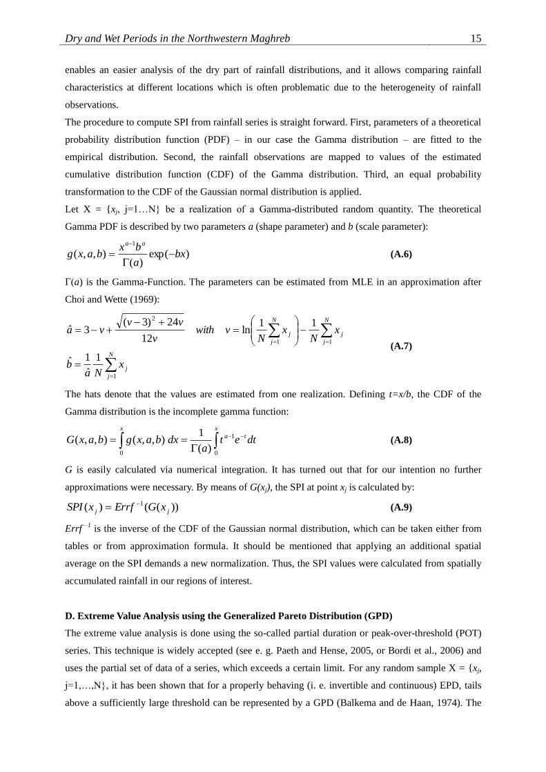
Dry and Wet Periods in the Northwestern Maghreb 15
enables an easier analysis of the dry part of rainfall distributions, and it allows comparing rainfall
characteristics at different locations which is often problematic due to the heterogeneity of rainfall
observations.
The procedure to compute SPI from rainfall series is straight forward. First, parameters of a theoretical
probability distribution function (PDF) – in our case the Gamma distribution – are fitted to the
empirical distribution. Second, the rainfall observations are mapped to values of the estimated
cumulative distribution function (CDF) of the Gamma distribution. Third, an equal probability
transformation to the CDF of the Gaussian normal distribution is applied.
Let X = {xj, j=1…N} be a realization of a Gamma-distributed random quantity. The theoretical
Gamma PDF is described by two parameters a (shape parameter) and b (scale parameter):
)exp()(
),,(1
bxa
bxbaxg
aa
(A.6)
Γ(a) is the Gamma-Function. The parameters can be estimated from MLE in an approximation after
Choi and Wette (1969):
N
j
j
N
j
j
N
j
j
xNa
b
xN
xN
vwithv
vvva
1
11
2
1
ˆ
1ˆ
11ln
12
24)3(3ˆ
(A.7)
The hats denote that the values are estimated from one realization. Defining t=x/b, the CDF of the
Gamma distribution is the incomplete gamma function:
x
ta
x
dteta
dxbaxgbaxG0
1
0)(
1),,(),,( (A.8)
G is easily calculated via numerical integration. It has turned out that for our intention no further
approximations were necessary. By means of G(xj), the SPI at point xj is calculated by:
))(()( 1
jj xGErrfxSPI (A.9)
Errf—1
is the inverse of the CDF of the Gaussian normal distribution, which can be taken either from
tables or from approximation formula. It should be mentioned that applying an additional spatial
average on the SPI demands a new normalization. Thus, the SPI values were calculated from spatially
accumulated rainfall in our regions of interest.
D. Extreme Value Analysis using the Generalized Pareto Distribution (GPD)
The extreme value analysis is done using the so-called partial duration or peak-over-threshold (POT)
series. This technique is widely accepted (see e. g. Paeth and Hense, 2005, or Bordi et al., 2006) and
uses the partial set of data of a series, which exceeds a certain limit. For any random sample X = {xj,
j=1,…,N}, it has been shown that for a properly behaving (i. e. invertible and continuous) EPD, tails
above a sufficiently large threshold can be represented by a GPD (Balkema and de Haan, 1974). The

Dry and Wet Periods in the Northwestern Maghreb 16
GPD is a three-parameter distribution with probability density
01
011
),,,(
1
aforeb
aforb
cxa
bcbaxf
b
cx
a
a
(A.10)
and the cumulative distribution function
01
0)(
11),,(
1
afore
aforb
cxa
baxF
b
cx
a
(A.11)
The GPD is described by the location parameter c, the scale parameter b and the shape parameter a. It
is defined for any value x > c for a > 0 and c x c - b/a. F(x,a,b,c) is the probability that a value in
the tail of an EPD is larger than c and smaller than or equal to x. The GPD is an exponential
distribution for a = 0, a type II Pareto distribution for a < 0 and an ordinary Pareto distribution for
a > 0. The estimation of parameters of the GPD is not analytically possible; a brief overview of
methods is given in Singh and Guo (1995). In this study, the method of L-moments (Hosking and
Wallis, 1987) has been used. For that purpose, probability weighted moments m, m=0,..,2 were
calculated:
N
mj
jm
N
j
j
xrNNN
rjjj
N
xN
1
1
0
))...(2)(1(
))...(2)(1(1
1
(A.12)
From these moments, the L-moments have been computed:
0123
012
01
66
2
(A.13)
The parameters of the GPD were estimated by:
a
bc
aab
a
1
)2)(1(
3
1
2
32
32
(A.14)
The location parameter c is usually, except from numerical fluctuations, identical with the lowest value
of {X|xj > c}. Hosking and Wallis (1987) proved that for a large number of samples maximum
likelihood estimates of a and b are normally distributed. The estimation error a and b is expressed in
the approximated covariance matrix of a and b:

Dry and Wet Periods in the Northwestern Maghreb 17
22
22
2
2
2
2
)1(2)1(
)1()1(1
bab
aba
abab
aba
Nbba
baa
(A.15)
Here, the overbar denotes an average over the sample of (a,b). This error estimate may be a little bit
smaller for L-moments, but has been used to ensure that we are on the safe side. The error of the GPD
can now easily be derived from multivariate error propagation of the GPD f:
22
2
2
2
2 2 abbafb
f
a
f
b
f
a
f
(A.16)
The estimation of the optimum threshold for the GPD fit is very important for reliable results. It has
been shown that the mean residual life function (MRL, also known as mean excess function) has a
linear shape for sufficiently high thresholds. The MRL function is defined as:
)()(
1)(
)(
1
exN
i
i
ex
xN
MRL (A.17)
is the threshold, Nex() is the number of values exceeding . Because the fit is – in a statistically
sense – better when using more data, the threshold should be chosen to be in the linear range of the
MRL function, but as near to the centre of the distribution as possible. This is a somehow arbitrary
criterion, thus, the MRL was used in this study merely to control the estimation of the optimum
threshold.
Another method to estimate the threshold is based on the so-called quantile-quantile plot (QQ-plot). In
a QQ-plot, empirical cumulative probabilities are plotted against the GPD fit based on this threshold.
Supposed we have sufficiently GPD distributed sample data, the perfect fit would result in a straight
line of identity. A quality measure for the GPD fit is the mean integrated standard error (MISE):
)(
1
2))(),,(()(
exN
i
ii xECDbaxFMISE (A.18)
Here, ECD is the empirical cumulative distribution function. The MISE is – except to a constant factor
– a measure for the distance of the points from the line marking the identity. In our estimation of , the
threshold according to the minimum value of MISE for moving has been chosen.
The return levels are calculated from the inverse of the cumulative GPD Function. The probability,
that a random value xj taken from our sample in size N exceeds the threshold c is
N
NcxPp ex
jc )( (A.19)
The probability, that values in a GPD fit exceed an arbitrary value s >= x is
a
jjb
cxacxsxP
1
1)|(
(A.20)
This can be converted to

Dry and Wet Periods in the Northwestern Maghreb 18
a
cjb
cxapsxP
1
1)(
(A.21)
The level xt that in average is exceeded once in a time interval of t is the inversion of eq. (A.21):
1)( a
ct tpa
bcx (A.22)
Again, the standard error of xt obtained from error propagation in eq. (A.16).
22
2
2
2
2 2 ab
tt
b
t
a
t
xb
x
a
x
b
x
a
xt
(A.23)
with
1)(1
)(1
)log(1
a
ct
a
cct
tpaa
x
tpa
tpaa
b
a
x
(A.24)
The programs used in the present study to calculate the GPD fit are freely available under
https://wiki.uni-koeln.de/kerschgens/index.php/Kai_Born.
E. List of Abbreviations and Acronyms
The list is in alphabetical order.
ATL Atlantic coast region
CDF Cumulative distribution function
CRU Climate research unit of the university of East Anglia
CRU TS2.1 An observational climate data set provided by the CRU
ECD Empirical cumulative distribution
ECHAM European Center for Medium Ragne Weather forecast model – Hamburg version
ENSO El Niño-Southern Oscillation
EPD Empirical distribution function
FAO Food and Agriculture Organization of the United Nations
GCM General circulation model
GHCN Global historical climatology network, produced jointly by the National Climatic Data
Center and Carbon Dioxide Information Analysis Center at Oak Ridge National Laboratory
GHG Greenhouse gas
GPD Generalized distribution function
IMPETUS Integratives Management-Projekt für einen effizienten und tragfähigen Umgang mit
Süßwasser in Westafrika
An Integrated Approach to the Efficient Management of Scarce Water Resources in West
Africa
IPCC Intergovernmental Panel on Climate Change
KCD Kernel estimated cumulative probability distribution
KPD Kernel estimated probability distribution
LCC Land cover changes
MED Mediterranean cost region
MISE Mean integrated standard error
MLE Maximum likelihood estimation
MPIfM Max Planck Institute for Meteorology, Hamburg
MRL Mean residual life function
NAO North Atlantic Oscillation
NCAR National Center for Atmospheric Research, Boulder, Colorado, USA
NCEP National Centers for Environmental Predictions, Camp Springs, Maryland ,USA

Dry and Wet Periods in the Northwestern Maghreb 19
OAGCM Ocean-Atmosphere general circulation model
PCA Principal component analysis
PDF Probability distribution function
POT Peak-over-threshold method: only values exceeding a fixed threshold are taken into
consideration
PP Principal pattern
QI Quintile index
QQ-plot Quantile-quantile plot
RCM Regional climate model
REMO Regional Model: A meso-sale amospheric model for regional climate modelling applications
SOA South of the Atlas region
SPI Standardized precipitation index
SRES Special Report on Emissions Scenarios of the IPCC
SST Sea Surface Temperature
SYNOP Synoptic weather observations
VASCLIMO Variability Analysis of Surface Climate Observations: A joint project between the German
Weather Service DWD and the Institute for Meteorology and Geophyiscs, Johann Wolgang
Goethe University Frankfurt
Acknowledgements
This work was part of the IMPETUS West-Africa project and was supported by the Federal German Ministry of
Education and Research (BMBF) under grant No. 01 LW 06001A in the GLOWA programme and by the
Ministry of Innovation, Science, Research and Technology (MIWFT) of the federal state of Northrhine-Westfalia
under grant No. 313-21200200.
The observational data were collected and maintained under the participation of Tim Brücher and Kristina Piecha
from the Institute for Geophysics and Meteorology of the University Cologne. The SPI analysis has been
supported by the work of Rabea Haas, University of Cologne. Robin Girmes and Kai-Oliver Heuer, who were
involved in the IMPETUS project, have supplied model data management. Daniela Jacob and Ralf Podzun, Max-
Panck-Institute for Meteorology in Hamburg, have realized the RCM model runs at the Deutsches
Klimarechenzentrum. We are grateful to two anonymous reviewers for their rewarding comments.

Dry and Wet Periods in the Northwestern Maghreb 20
References
Beck, C., J. Grieser, B. Rudolf, 2005: A New Monthly Precipitation Climatology for the Global Land Areas for
the Period 1951 to 2000. Published in Climate Status Report 2004, pp. 181 - 190, German Weather Service,
Offenbach, Germany.
Balkema, A. A., L. de Haan, 1974: Residual life time at great age. -- Annals of Probability 2, 792-804.
Bordi, I., A. Sutera, 2001: Fifty years of precipitation: Some spatially remote teleconnections. -- Water Res.
Management, 15, 247-280.
Bordi, I., K. Fraedrich, M. Petitta, A. Sutera, 2006: Extreme value analysis of wet and dry periods in Sicily. --
Theor. Appl. Climatol. (2006), DOI 10.1007/s00704-005-0195-3.
Choi, S. C., R. Wette, 1969: Maximum Likelihood Estimation of the Parameters of the Gamma Distribution and
Their Bias. -- Technometrics, 11(4), 683-690-
El Hamly, M., Sebbari, R., Lamb, P. J., Ward, M. N., D. H. Portis, 1998: Towards the seasonal prediction of
Moroccan precipitation and its implication for water resources management. -- Water Resources Variabilty in
Africa during the XXth century, Proceedings of the Abidjan 1998 Conference, Abidjan, Côte d’Ivoire, 1998.
IAHS Publ. No. 252, 79-87.
Emberger, L., 1930 : La végétation de la région méditerranéenne; essai de classification des groupements
végétaux. 1930. -- Rev. Gen. de Bot., 42, 641-662.
Emberger, L., 1955 : Une classification biogéographique des climats. -- Recueil Trav. Lab. Bot. Géol. Zool. Fac.
Sci. Univ. Montpellier, Serie Bontanique, 7, 3-43.
Finckh, M., A. Augustin, N. Jürgens, 2007: Monitoring biodiversity on the Saharan slopes of the High Atlas,
Morocco. -- Mountain Forum Bulletin 2007 (1), 3-4.
Fraedrich, K., F.-W. Gerstengarbe, P. C. Werner, 2001: Climate shift during the last century. --Climatic Change,
50, 405-417.
Griffiths, F., 1972: The Mediterranean Zone. -- Chapter 2 in World Survey of Climatology Vol 10: Climates of
Africa. Ed. H. E. Landberg. Elsevier Publishing Company Amsterdam – London – New York, 37-74.
Griffiths, F., K. H. Soliman, 1972: The Northern Desert (Sahara). -- Chapter 3 in World Survey of Climatology,
Vol 10: Climates of Africa. Ed. H. E. Landberg. Elsevier Publishing Company Amsterdam – London – New
York, 75-132.
Guetter, P. J., Kutzbach, J. E., 1990: A modified Koeppen classification applied to model simulations of glacial
and interglacial climates. -- Clim. Change, 16, 193-215.
Guttmann, N. B., 1999: Accepting the standardized precipitation index: a calculation algorithm. -- J. Amer. Water
Resources Assn., 35, 311-322.
Hosking, J., J. Wallis, 1987: Parameter and quantile estimation for the generalized Pareto distribution. --
Technometrics, 29, 339-349.
Hotelling, H., 1933: Analysis of a complex of statistical variables into principal components. -- J. Educ.
Psychol., 24, 417-441.
IPCC, 2007: IPCC Fourth Assessment Report (AR4) Working Group I Report "The Physical Science Basis",
available online http://ipcc-wg1.ucar.edu/wg1/wg1-report.html (Sep 16, 2007).
Jacob, D., Van den Hurk, B.J.J.M., Andrae, U., Elgered, G., Fortelius, C., Graham, L.P., Jackson, S.D., Karstens,
U., Koepken, C., Lindau, R., Podzun, R., Rockel, B., Rubel, F., Sass, B.H., Smith, R., Yang, X., 2001, A
comprehensive model intercomparison study investigating the water budget during the PIDCAP period. --
Meteorol. Atmos. Phys. 77, 19-44.
Jung, T., L. Ferranti, A. M. Tompkins, 2006: Response of the Summer of 2003 Mediterranean SST Anomalies
over Europe and Africa. -- J. Climate 19, 5439-5454.
Knippertz, P.; Christoph, M.; Speth, P., 2003: Long-term precipitation variability in Morocco and the link to the
large-scale circulation in recent and future climates. -- Meteorology and Atmospheric Physics, 83, 67–88.
Knippertz, P., 2004: A simple identification scheme for upper-level troughs and its application to winter
precipitation variability in Northwest Africa. -- J. Climate, 17, pp. 1411-1418.
Köppen, W., 1936: Das geographische System der Klimate. -- In: Handbuch der Klimatologie, Vol. 1, Part C,
Gebr. Bornträger Verlag Berlin, 388 pp. (in German)

Dry and Wet Periods in the Northwestern Maghreb 21
Kottek, M., J. Grieser, C. Beck, B. Rudolf, F. Rubel, 2006: World map of the Köppen-Geiger climate
classification updated. -- Meteorol. Z., 15, 259-263.
Lamb, P.J., R. A. Peppler, 1987: North Atlantic Oscillation: concept and application. -- Bull. Amer. Met. Soc. 68,
1218–1225.
Lamb P.J, M. El Hamly, D. H. Portis DH, 1997: North-Atlantic Oscillation. -- Géo Observateur 7, 103–113.
Li, S., W. A. Robinson, S. Peng, 2003: Influence of the North Atlantic SST tripole on northwest African rainfall.
-- J. Geophys. Res. 108(D19), ACL 3, 1-20, doi: 10.1029/2002JD003130.
McKee, T. B., N. J. Doesken, J. Kleist, 1993: The relationship of drought frequency and duration to time scales. -
- Preprints, 8th
Conference on Applied Climatology, Jan. 17-22, Anaheim, CA, 179-184.
Mitchell, T. D., P. D. Jones, 2005: An improved method of constructing a database of monthly climate
observations and associated high resolution grids. -- Int. J. Climatol. 25, 693-712.
Murtagh, F., 2007: Multivariate Data Analysis Software and Resources. -- Available under http://astro.u-
strasbg.fr/~fmurtagh/mda-sw/, 25.8.2007.
Nicholson, S. E., 2000: The nature of rainfall variability over Africa on time scales of decades to millennia. --
Global and Planetary Change 26, 137-158.
Paeth, H., 2004: Key factors in African climate change evaluated by a regional climate model. -- Erdkunde 58,
290-315.
Paeth, H., K. Born, R. Podzun, D. Jacob, 2005, Regional dynamic downscaling over West Africa: Model
evaluation and comparison of wet and dry years. -- Meteorol. Z. 14, 349-367.
Paeth, H., Hense, A., 2005: Mean versus extreme climate in the Mediterranean region and its sensitivity to future
global warming conditions. -- Meteorol. Z. 14, 329-347.
Paeth, H., K. Born, R. Girmes, R. Podzun, D. Jacob, 2008: Regional Climate change in tropical and northern
Africa due to greenhouse forcing and land use changes. -- Accepted in J. Climate.
Palmer, W., 1965: Meteorological Drought. -- Tech. Rep. 45, U.S. Weather Bureau, Washington D.C., 58 pp.
Pearson, K., 1901: On lines and planes of closest fit to systems of points in space. -- Philos. Magazine 2, 559-
572.
Portis D. H., J. E. Walsh, M. El Hamly, P. J. Lamb, 2001: Seasonality of the North Atlantic Oscillation. -- J.
Climate 14, 2069–2078
Preisendorfer, R. W., 1988: Principal component analysis in meteorology and oceanography. -- In: C. D. Mobly
(ed.), Developments in Atmospheric Sciences, 17, 425 pp.
Roeckner, E. et al., 2003. The atmospheric general circulation model ECHAM 5. PART I: Model description.--
MPI-Report 349, 127pp (2003).
Singh, V, P., H. Guo, 1995: Parameter estimation for 3-parameter generalized pareto distribution by the principle
of maximum entropy (POME). -- Hydrological Sciences Journal 40, 165-181.
Vose R. S., R. L. Schmoyer, P. M. Steurer, T. C. Peterson, R. Heim, T. R. Karl, J. K. Eischeid, 1992: The Global
Historical Climatology Network: Long-term monthly temperature, precipitation, sea level pressure, and station
pressure data. -- NDP-041. Carbon Dioxide Information Analysis Center, Oak Ridge National Laboratory, Oak
Ridge, Tennessee
Ward, M. N., P. J. Lamb, D. H. Portis, M. El Hamly, R. Sebbari, 1999: Climate variability in northern Africa:
understanding droughts in the Sahel and the Maghreb. -- Chapter 6 in: Beyond El Niño – decadal and
interdecadal climate variability. Ed.: A. Navarra. Springer Verlag, 119-140.
WMO, World Meteorological Organization, 1983: Guide to climatological practices. Secretariat of the World
Meteorological Organization, Geneva, Switzerland. -- WMO No. 100, Second Edition 1983, 198 pp.

Dry and Wet Periods in the Northwestern Maghreb 22
Fig.1: SYNOP Stations in the north-western Maghreb. Circles represent the locations of the
stations, numbers the observed 1951-2000 mean annual rainfall sum in mm.

Dry and Wet Periods in the Northwestern Maghreb 23
Fig. 2: Climate classification after a reduced Köppen scheme applied to the CRU TS2.1 data. The maps compare
the climate classes for 1951-1965 to 1986-2000 and reveal a trend towards dryer and warmer climates in the
second half of the 20th
century. Classification criteria are listed in Table 1.

Dry and Wet Periods in the Northwestern Maghreb 24
Fig. 3: Climate classification after Köppen for simulated climate scenarios from REMO.

Dry and Wet Periods in the Northwestern Maghreb 25
Fig. 4: The leading eight principal patterns (PP) of the PCA for the period 1951-2000.
Continuous contour lines and light grey shading indicate positive, dashed lines and darker
grey shading negative values. The numbers in the upper left corners show the explained
variance (EV) and the cumulative explained variance (CV) of the first PPs. The PPs are
multiplied with the root of the according eigenvalue, so that they represent the correlation
patterns. From the first three patterns three characteristic regions are defined: PP01->ATL
(Atlantic region), PP02-> SOA (south of the Atlas Mountains) and PP03-> MED
(Mediterranean region).

Dry and Wet Periods in the Northwestern Maghreb 26
Fig. 5: Eigenvalues of the PCA (grey circles with error estimates) vs. randomly generated
eigenvalues (straight line with broken lines for error estimates). The application of
Preisendorfers Rule N shows that only the first three PPs emerge from random noise.

Dry and Wet Periods in the Northwestern Maghreb 27
Fig. 6: Time series of annual SPI values obtained from GHCN station data for the period
1901/2-2006/7 for the Atlantic (ATL), Mediterranean (MED) on southern (SOA) regions. Grey
bars: Index values, white bars: number of available stations for each region. As a measure of
variability within the regions, the vertical lines centred at the grey bars denote the standard
deviation of SPI values of single stations inside each region.

Dry and Wet Periods in the Northwestern Maghreb 28
Fig. 7: Same as Fig. 6, for CRU TS2.1. In the lower part of the panels, time-series of the
correlation between SPI values calculated from CRU TS2.1 and GHCN data in a shifting 31-
year-window are shown.

Dry and Wet Periods in the Northwestern Maghreb 29
Fig. 8: Annual SPI values from RCM model runs. In order to enhance the quality of the
statistical procedure, all data were collected into one time series of 422 years length. Vertical
straight lines mark the intersection between experiments; the labels at bottom axis denote the
names of the experiments. C20-1 is the first 1961-2000 experiment, A1B-1 the first scenario
SRES A1B experiment and so on. Basis for the SPI calculation was the whole dataset.

Dry and Wet Periods in the Northwestern Maghreb 30
Fig. 9: Exemplary results of the extreme value analysis for the GHCN data for the period
1901/2-2006/7, for the three regions ATL, MED and SOA.
Top row: The MRL functions and MISE calculated from EDF and from Gaussian kernel
estimation. Vertical axes show on the left side MRL in SPI units, on the right side MISE in SPI
units.
Second Row: Distributions, EDF and KDF from SPI data. In addition, the scaled GPD fit to
the tails has been added together with the estimated 95% uncertainty. The vertical axis shows
probability.
The two bottom rows: Return values obtained from ECD (squares), kernel estimated KCD
(broken line) and from GPD analysis (thick lines with broken lines showing the 95%
uncertainty range). On the horizontal axes, years are shown, on the vertical SPI units. For the
graphics, dry SPI values are changed in sign.

Dry and Wet Periods in the Northwestern Maghreb 31
Fig. 10: Return values of the SPI estimated from RCM compared to values from GHCN
observations. For the graphics, the dry SPI values are changed in sign.
Two upper rows: Wet and dry return values from calculations using empirical and kernel
estimated return values on SPI time series. Shown are empirical GHCN observations (1902-
2007), kernel estimated GHCN observations (1902-2007), CRU TS2.1, REMO all (1961-
2050), REMO C20 (1961-2000) present day climate simulations and REMO A1B and B1
combined scenarios (2031-2050). The two bottom rows show return values obtained from
extreme value analysis using the GPD fit, only for REMO C20 and the combined scenarios
A1B and B1, again for 2031-2050. The broken lines in the left two columns mark the 95%
uncertainty levels.

Dry and Wet Periods in the Northwestern Maghreb 32
Table 1: Definition of classes of the reduced Köppen climate classification. T is the mean monthly temperature in
2m hight above ground, Prec is the annual precipitation sum. Max / Min T indicate the warmest and coldest
month in the mean annual cycle.
Name Climate Criterion 1 Criterion 2
E Ice Max T < 10°C
D Snow Max T > 10°C and Min T < -3°C
Cs Moderate -3°C < Min T < 18°C summer dry
Cf Wet
Cw winter dry
Af Tropical Min T > 18°C Wet
Am Monsoon climate*
Aw/s
winter/summer dry
BSk Steppe {Mean T} < {Prec} < 2 {Mean T} cold (Mean T < 18°C)
BSh warm (Mean T > 18°C)
BWk Desert cold with Mean T < 18°C
BWh warm with Mean T > 18°C
* In monsoon climates, the dry period is compensated by annual rainfall: let pmin be the rainfall of the driest month, then pmin is
compensated if Prec > 2500-500*(pmin / 20)
Table 2: Short description of SRES scenario families. The scenarios chosen for future climate scenarios in
IMPETUS are shaded.
A
Rapid economic growth
B
Environmental sustainable development
Glo
ba
l
A1 Globally uniform development:
Rapid economic growth, low population
growth and rapid introduction of more
efficient technologies
B1 As A1, but with rapid changes in
economic structures toward a service and
information economy, with reductions in
material intensity, and the introduction of
clean and resource-efficient technologies. A1B As A1, but with a future energy source mix
which does not depend on one particular
energy source.
Reg
ion
al
A2 Regional heterogeneous development:
High population growth. Economic
development primarily regionally oriented.
Economic growth and technological
change are more fragmented and slower
than in A1.
B2 Emphasis is on local solutions to
economic, social, and environmental
sustainability. Moderate population
growth, intermediate economic
development, less rapid and more diverse
technological change. Focussing on local
and regional levels.