Institutionen för systemteknikDepartment of Electrical Engineering

Examensarbete

Double Differential TOA Positioning for GSM

Examensarbete utfört i Kommunikationssystemvid Tekniska högskolan vid Linköpings universitet

av

Andreas Nordzell

LiTH-ISY-EX--13/4681--SE

Linköping 2013

Department of Electrical Engineering Linköpings tekniska högskolaLinköpings universitet Linköpings universitetSE-581 83 Linköping, Sweden 581 83 Linköping

Double Differential TOA Positioning for GSM

Examensarbete utfört i Kommunikationssystemvid Tekniska högskolan vid Linköpings universitet

av

Andreas Nordzell

LiTH-ISY-EX--13/4681--SE

Handledare: Mirsad Čirkic, Doktorandisy, Linköpings universitet

Anders Johansson, PhDFOI

Examinator: Danyo Danevisy, Linköpings universitet

Linköping, 17 juni 2013

Avdelning, InstitutionDivision, Department

Division for Communication SystemsDepartment of Electrical EngineeringSE-581 83 Linköping

DatumDate

2013-06-17

SpråkLanguage

� Svenska/Swedish

� Engelska/English

�

�

RapporttypReport category

� Licentiatavhandling

� Examensarbete

� C-uppsats

� D-uppsats

� Övrig rapport

�

�

URL för elektronisk version

http://urn.kb.se/resolve?urn=urn:nbn:se:liu:diva-94162

ISBN

—

ISRN

LiTH-ISY-EX--13/4681--SE

Serietitel och serienummerTitle of series, numbering

ISSN

—

TitelTitle

Dubbel Differentiell TOA Positionering för GSM

Double Differential TOA Positioning for GSM

FörfattareAuthor

Andreas Nordzell

SammanfattningAbstract

For most time-based positioning techniques, synchronization between the objects in the sys-tem is of great importance. GPS (global positioning system) signals have been found veryuseful in this area. However, there are some shortcomings of these satellite signals, makingthe system vulnerable. The aim of this master thesis is to investigate an alternative methodfor synchronization, independent of GPS signals, which could be used as a complement. Theproposed method takes advantage of the broadcast signals from telecommunication towers,and use them for calculation of the synchronization error between two receivers. By lookingat the time difference between arrival times at the receivers, and compare it to the true timedifference, the synchronization error can be found. A precondition is that the locations ofthe receivers as well as the tele tower are known beforehand, so that the true time differencecan be calculated using geometry.

The arrival times are determined through correlation between the received signals andknown training bits, which are a part of the transmission sequence. For verification, ex-periments were made on localization of a mobile phone in the GSM (global system of mobilecommunications) network.

This research was a collaboration with FOI, the Swedish Defense Research Agency, wheremost of the work was done.

NyckelordKeywords TOA, TDOA, Mobile Positioning, GSM

Till Maja, Sanna, Jonas, Vedran, Björn och Johan.Utan er hade det nog gått ändå...

iii

Abstract

For most time-based positioning techniques, synchronization between the objectsin the system is of great importance. GPS (global positioning system) signalshave been found very useful in this area. However, there are some shortcomingsof these satellite signals, making the system vulnerable. The aim of this masterthesis is to investigate an alternative method for synchronization, independent ofGPS signals, which could be used as a complement. The proposed method takesadvantage of the broadcast signals from telecommunication towers, and use themfor calculation of the synchronization error between two receivers. By looking atthe time difference between arrival times at the receivers, and compare it to thetrue time difference, the synchronization error can be found. A precondition isthat the locations of the receivers as well as the tele tower are known beforehand,so that the true time difference can be calculated using geometry.

The arrival times are determined through correlation between the received sig-nals and known training bits, which are a part of the transmission sequence. Forverification, experiments were made on localization of a mobile phone in theGSM (global system of mobile communications) network.

This research was a collaboration with FOI, the Swedish Defense Research Agency,where most of the work was done.

v

Acknowledgments

My sincere and most grateful thank you goes to ...

...my supervisor Anders Johansson and project manager Patrik Hedström at FOI,for the countless hours you have spent helping me through insightful discussions,with cables and wires, with report reflections and last but not least, to execute thefield experiment. Without your help and support, I would never have reached mygoal.

...my supervisor Mirsad Čirkić, for constructive critics during the work with thisreport, as well as the long repetition course in Gaussian distribution calculationsand the Q-function.

...my examiner Danyo Danev, for many inspiring courses in the field of com-munication systems, and for helping me become a Master of science in AppliedPhysics and Electrical Engineering.

Linköping, June 2013Andreas Nordzell

vii

Content

Symbols xi

Abbreviations xiii

1 Introduction 11.1 Thesis Description . . . . . . . . . . . . . . . . . . . . . . . . . . . . 11.2 Synchronization and the Importance of Accuracy . . . . . . . . . . 21.3 Restrictions . . . . . . . . . . . . . . . . . . . . . . . . . . . . . . . . 31.4 The Matter of No GPS . . . . . . . . . . . . . . . . . . . . . . . . . . 31.5 Previous Work . . . . . . . . . . . . . . . . . . . . . . . . . . . . . . 31.6 Outline . . . . . . . . . . . . . . . . . . . . . . . . . . . . . . . . . . 4

2 Theory 52.1 GSM . . . . . . . . . . . . . . . . . . . . . . . . . . . . . . . . . . . . 5

2.1.1 General Information . . . . . . . . . . . . . . . . . . . . . . 52.1.2 Transmission Rate and Bandwidth . . . . . . . . . . . . . . 52.1.3 Time Division Multiple Access . . . . . . . . . . . . . . . . 72.1.4 Frame Structure . . . . . . . . . . . . . . . . . . . . . . . . . 72.1.5 Burst Structure . . . . . . . . . . . . . . . . . . . . . . . . . 72.1.6 Frequency Hopping . . . . . . . . . . . . . . . . . . . . . . . 82.1.7 Transmission and Reception . . . . . . . . . . . . . . . . . . 82.1.8 Modulation . . . . . . . . . . . . . . . . . . . . . . . . . . . 9

2.1.8.1 Gaussian Minimum Shift Keying . . . . . . . . . . 92.1.8.2 Differential Encoding . . . . . . . . . . . . . . . . 92.1.8.3 Gaussian Filtering . . . . . . . . . . . . . . . . . . 102.1.8.4 Phase Function . . . . . . . . . . . . . . . . . . . . 10

2.1.9 Relevant Information . . . . . . . . . . . . . . . . . . . . . . 112.1.10 Training Sequences . . . . . . . . . . . . . . . . . . . . . . . 11

2.2 Time-Based Localization . . . . . . . . . . . . . . . . . . . . . . . . 122.2.1 Time Difference of Arrival . . . . . . . . . . . . . . . . . . . 122.2.2 Time of Arrival . . . . . . . . . . . . . . . . . . . . . . . . . 132.2.3 Double Differential Time of Arrival . . . . . . . . . . . . . . 14

2.2.3.1 Calculating the Time Difference . . . . . . . . . . 15

ix

x CONTENT

2.2.3.2 Evaluation of Bound for Synchronization Error . . 16

3 Method 193.1 Correlation . . . . . . . . . . . . . . . . . . . . . . . . . . . . . . . . 19

3.1.1 Mathematical Description . . . . . . . . . . . . . . . . . . . 203.1.2 Comments on Accuracy . . . . . . . . . . . . . . . . . . . . 22

3.2 Curve Fitting . . . . . . . . . . . . . . . . . . . . . . . . . . . . . . . 233.3 Averaging . . . . . . . . . . . . . . . . . . . . . . . . . . . . . . . . . 233.4 Implementation . . . . . . . . . . . . . . . . . . . . . . . . . . . . . 23

3.4.1 Demodulation and Frequency Correction . . . . . . . . . . 233.4.2 Practical Aspects . . . . . . . . . . . . . . . . . . . . . . . . 243.4.3 Discrete Correlation . . . . . . . . . . . . . . . . . . . . . . 243.4.4 Interpolation . . . . . . . . . . . . . . . . . . . . . . . . . . . 253.4.5 Modulated Training Sequence . . . . . . . . . . . . . . . . . 253.4.6 Algorithms . . . . . . . . . . . . . . . . . . . . . . . . . . . . 26

4 Simulation 294.1 System Model . . . . . . . . . . . . . . . . . . . . . . . . . . . . . . 294.2 Calculations . . . . . . . . . . . . . . . . . . . . . . . . . . . . . . . 294.3 Results . . . . . . . . . . . . . . . . . . . . . . . . . . . . . . . . . . 31

5 Laboratory Trials and Field Test 375.1 Receiver Hardware . . . . . . . . . . . . . . . . . . . . . . . . . . . 375.2 TEMS Mobile Phone . . . . . . . . . . . . . . . . . . . . . . . . . . . 385.3 Execution . . . . . . . . . . . . . . . . . . . . . . . . . . . . . . . . . 38

5.3.1 Laboratory Setup . . . . . . . . . . . . . . . . . . . . . . . . 405.3.2 Field Test Setup . . . . . . . . . . . . . . . . . . . . . . . . . 41

5.4 Results . . . . . . . . . . . . . . . . . . . . . . . . . . . . . . . . . . 435.4.1 Received Signals . . . . . . . . . . . . . . . . . . . . . . . . . 435.4.2 Laboratory Trials . . . . . . . . . . . . . . . . . . . . . . . . 435.4.3 Field Test . . . . . . . . . . . . . . . . . . . . . . . . . . . . . 475.4.4 Comments on Results . . . . . . . . . . . . . . . . . . . . . . 48

6 Conclusions 536.1 Results . . . . . . . . . . . . . . . . . . . . . . . . . . . . . . . . . . 536.2 Suggested Improvements . . . . . . . . . . . . . . . . . . . . . . . . 536.3 Future Developments . . . . . . . . . . . . . . . . . . . . . . . . . . 546.4 Final Comments . . . . . . . . . . . . . . . . . . . . . . . . . . . . . 54

List of Figures 55

List of Tables 58

Bibliography 59

Symbols

In order of appearance

Notation Descriptions(t) Signal sentt, τ Time variableEb Bit (symbol) energyT Symbol period (≈ 3.69 microseconds)fc Carrier frequencyϕ(t) Phase functionb Information bitd Differential encoded bitα Information symboli, j Indexg(t) Gaussian filter (frequency function)h(t) Gaussian distribution

rect(t) Rectangle functionexp(t) Exponential functionσ Standard deviationBh 3 dB bandwidth of h(t)µ Modulation indexw White Gaussian noisex(t) Received signal∆, δ Time delayr(τ) Cross correlation functionS(f ) Cross spectraE[ · ] Expected valueF { · } Fourier transformf Frequency variablec Propagation speed of light in air

Px Position of object x

xi

xii Symbols

Notation DescriptionMs Mobile station (transmitter to be located)Bs Base station (reference source)Rx1 Receiver 1Rx2 Receiver 2ρ Circle radiusτx,y The time instant for when a signal sent from object x

arrives at object y (Time Of Arrival)TP Time period between two consecutive training se-

quencesεsync Synchronization errory(t) Random signalL Length of a training sequenceB Bandwidth

sinc(t) Sinc function (normalized)a constantM Number of TOA estimations used for averagingr[n] Discrete time estimation of the cross correlation func-

tionn Discrete time variableN Number of recorded samplesσ2 Standard deviationΛ Oversampling rate

xtr[n] Complex baseband representation of the modulatedtraining sequence

Imaginary unit (2 = −1)foffset Frequency offsetx[n] Training sequence with added WGNτerror TOA errorεtoa RMS for the TOA estimationNest Number of estimations used for a RMS calculation

∆error DDTOA errorξ Normal distribution variableχ Normal distribution variable

εddtoa RMS for the DDTOA estimationFd Downlink carrier frequencyFs Sample frequencyFu Uplink carrier frequency

Abbreviations

In alphabetic order

Acronym DescriptionAM Amplitude ModulationALE Adaptive Line EnhancerAOA Angle Of Arrival

ARFCN Absolute Radio Frequency Channel NumberAWGN Addative White Gaussian Noise

A/D Analog/DigitalBCC Base station Color CodeBSIC Base Station Identity CodeCCH Control ChannelCPM Continuous Phase ModulationDDC Digital Downconverter

DDTOA Double Differential Time Of Arrival (!)DL Downlink

DTOA Differential Time Of ArrivalEDGE Enhanced Data rates for GSM evolutionETSI European Telecommunications Standards Institute

FCCH Frequency Correction ChannelFN TDMA Frame NumberFOI Totalförsvarets Forskningsinstitut (Swedish Defense

Research AgencyGMSK Gaussian Minimum Shift KeyingGPRS General Packet Radio ServiceGPS Global Positioning SystemGSM Global System of Mobile communication

I IdleIF Intermediate Frequency

I/Q In-phase/Quadrature-phase

xiii

xiv Abbreviations

Acronym DescriptionLOS Line Of SightNCC Network Color CodePPS Pulse Per SecondRF Radio Frequency

RMS Root Mean Square errorRSS Received Signal StrengthSCH Synchronization ChannelSNR Signal to Noise Ratio

TDMA Time Division Multiple AccessTDOA Time Difference Of ArrivalTEMS Test Mobile SystemTOA Time Of ArrivalTS0 Time Slot 0 in a TDMA frameUL Uplink

UWB Ultra-Wideband

1Introduction

Everybody who has been trying to find their way in an unfamiliar city by car,knows how useful it can be with a GPS (global positioning system) device. It iseasy to update the map, and you don’t have to stop every other turn to have alook at your directions. However, what happens when you drive into a tunnel?The author certainly knows from a few years back when he was working in Oslo,the capital of Norway, as a delivery man. Oslo has a lot of long tunnels withmany different exit points. And how will you know what exit to take when theGPS stops working as soon as you get underground? This is not the questionto be answered in this master thesis, yet, it gives a good example of one of theshortcomings of a GPS; namely the importance of a line of site (LOS) signal fromthe satellites. It can be difficult to use a GPS device indoor, or even in an urbanenvironment with a lot of adjacent buildings and high skyscrapers.

From an electronic warfare point of view, which is the main field for this masterthesis, the GPS signals can also easily be jammed or "spoofed" by the enemy. Thiscan cause trouble with self-positioning and time synchronization.

This master thesis will be dealing with the troubles of time synchronization whentrying to localize the origin of a radio signal. The time difference of arrival(TDOA) system normally use GPS signals for synchronization of the receivers.Here, a variation of TDOA will be introduced and analyzed, that uses signals ofopportunity instead of a GPS for time synchronization.

1.1 Thesis Description

The system setup can be seen in Figure 1.1. It consists of two receivers, one ref-erence source and one transmitter to be located. More precise, the target in this

1

2 1 Introduction

Figure 1.1: Overview of the system.

case will be a mobile phone, and the reference source is a telecommunicationstower (base station). The goal will be to find the location of the mobile using thedifference in time of arrival (TOA)1 at the receivers. Signals from the telecom-munications tower will be used for the synchronization. More on this in Section2.2.

The signals will be analyzed in the global system for mobile communication(GSM) standard. The reason for this choice over the maybe more up to datechoices 3G or 4G is due to the authors prior knowledge of GSM, and also becauseof its less complex structure.

The exact location will not be of interest, instead only the hyperbola (Section 2.2)of possible positions will be calculated and the positioning error will be examinedwith respect to this curve.

1.2 Synchronization and the Importance of Accuracy

Since radio signals are traveling in the speed of light in air, it is easy to show theimportance of accurate calculations of the time differences and thereby the timeof arrival. The same argument also explains the reason for the time synchroniza-tion. This will be illustrated with an example.

1.1 ExampleImagine that two receivers, A and B, are located 400 m apart, and the mobile 300m away from A in an orthogonal direction of B. The distance to B is then 500m by Pythagoras’. The difference in distance is 200 m, and the time differenceapproximately 0.67 µs when dividing by the speed of light. This indicates thatan error in time of arrival by the size of only 0.1 µs is enough to end up far fromthe true difference in distance.

1TOA means the time instant (or time stamp) for when the signal is detected at the receiver.

1.3 Restrictions 3

How accurate one can determine the time of arrival is a matter of available band-width, the signal to noise ratio (SNR), the length of the signal and the receiverhardware. More on this in Chapter 3.

1.3 Restrictions

The system will only deal with the direct LOS signals. The reflected ones, as wellas the attenuation factor, will be considered as noise in the model. Moreover, allpositions, except for the transmitter, are assumed to be known beforehand. Theyare also seen as stationary, meaning, none of the objects in the system are moving.

Calculations of the time differences will not be done in real time, making thematter of fast and efficient algorithms less important. The signals will be storedon file, and then processed. In an actual electronic warfare situation, the commu-nication between the two receivers (or between a receiver and a third party) aresupposed to be minimal. This fact is noted, but will not be of great importancefrom a practical point of view.

1.4 The Matter of No GPS

Although the whole point of this master thesis is to reduce the dependency of aGPS for time synchronization, the GPS will be used when collecting data duringthe field test. First, to determine the exact location of the receivers, the referencesource and also for verification of the mobile position. Second, to be able toanalyze the accuracy of the calculations.

The author is well aware of the irony in this, but the use of a GPS simplifiesthe work a lot. Approaches on self-positioning without GPS can be found in[Vidyarthi, 2012] or [Yan and Fan, 2008].

1.5 Previous Work

A large number of articles and technical reports have been written in the fieldof localization techniques. In [Gustafsson and Gunnarsson, 2005], the most com-mon methods, such as TOA, TDOA, angle of arrival (AOA) or received signalstrength (RSS), are briefly described and compared. The article is a few years old,but gives a good overview of mobile positioning, both in the static and in the dy-namic case (through filter estimation). [Gezici et al., 2005] also gives a good gen-eral description (although in Ultra-wideband (UWB) systems), along with someperformance bounds.

[Shahabi et al., 2011] show a way of improving the performance in a TDOA sys-tem, by the use of an adaptive line enhancer (ALE). ALE is a way of reducing thenoise and thereby increasing the SNR.

In [Yan and Fan, 2008], a way of co-locating a number of asynchronous receivers

4 1 Introduction

is presented. This TDOA system is also independent of GPS and relies on signalsof opportunity. The performance is tested using both digital TV signals and AM(amplitude modulation) signals as a reference source.

As a contrast to the asynchronous systems, [Yoon et al., 2012] presents a methodfor synchronizing the receivers in a TDOA system. This method uses a GPS to-gether with high performance oscillators and efficient signal processing to createprecise time synchronization. This article can be good for comparing synchro-nized and non-synchronized systems.

1.6 Outline

After this introduction, an overview of GSM is presented. It describes the nec-essary parts for this thesis work. Chapter 2 also includes the theory behind thepositioning system, together with the equation used to calculate the time delaybetween the two receivers. Chapter 3 continues by describing the methods tocalculate the time of arrivals, and how to implement them. In Chapter 4, somesimulation results are presented. These, quite simple, simulations were mademostly in order to test the methods. The laboratory trials and the field test areintroduced in Chapter 5. It describes the equipment that was used and the setup,together with the outcome and comments on the results. The final chapter sum-marizes the thesis, and a short section is given about the future work.

2Theory

This chapter describes the necessary theory. To start with, the basics of the GSMprotocol i presented, followed by different approaches on time-based localiza-tion.

2.1 GSM

In order to determine the time of arrivals, some basic knowledge about the GSMprotocol is needed, which will be presented in this section. It includes the partsof GSM that are closely related to the theory behind and implementation of thismaster thesis. The chapter should be considered as background information tohelp understand the rest of the thesis. Sections 2.1.9 and 2.1.10 are of specialinterest. For a deeper insight in GSM, see [3GPP, 2013].

2.1.1 General Information

The global standard for mobile communications, originally groupe spécial mo-bile, is the second generation protocol for mobile cellular networks. It was devel-oped by the european telecommunications standards institute (ETSI) in the late80’s and 90’s, to replace the analog first generation standard with a digital one.It was later expanded to include data communications via GPRS (general packetradio service) and EDGE (enhanced data rates for GSM evolution).

2.1.2 Transmission Rate and Bandwidth

The rate for which information is sent is 260’833 symbols/s, and the availablebandwidth is 200 kHz per carrier [3GPP, 2013].

5

6 2 Theory

0 1 2 3 4 204720462045

0 1 2 49 50

0 1 25

5049480 1 2 30 1 2 252423

0 1 2 3 4 5 6 7

1 burst

1 hyperframe = 2 048 superframes = 2 715 648 TDMA frames

1 superframe = 1 326 TDMA frames

1 (26-frame) multiframe 1 (51-frame) multiframe

1 TDMA frame

1 time slot = 156.25 symbols = 15/26 ms

(a) Overview

5049480 1 2 3

TS0 1 2 3 4 5 6 7

1 TDMA frame

TS0 1 2 3 4 5 6 7

1 TDMA frame

1 (51-frame) multiframe

TS0 1 2 3 4 5 6 7

1 TDMA frame

Control channel multiframe

0 1 2 3 504948

F S F S F SF S F S I

. . .

. . .

. . . . . . . . . . . . . . .

(b) CCH multiframe

Figure 2.1: (a) An overview of the frame structure of GSM. (b) Every 0’thslot in each TDMA frame is put together to create one control channel (CCH)multiframe. F = FCCH burst, S = SCH burst and I = Idle.

2.1 GSM 7

2.1.3 Time Division Multiple Access

The access scheme used in GSM is time division multiple access (TDMA). EachTDMA frame contains eigth physical channels (or time slots) per carrier. Onetime slot has a duration of 15/26 ms (≈ 576.9µs), and includes 156.25 symbols(in this case the same as bits, and the 1/4 bit is included in the guard period).These 156.25 bits are put together in a bit frame, known as a burst.

2.1.4 Frame Structure

The longest cycle of TDMA frames is called a hyperframe, and lasts for 3 h 28min 53 s and 760 ms. This hyperframe is divided into 2 715 648 TDMA frames,each with a specific TDMA frame number (FN).

The hyperframe contains 2048 superframes, which in turn contains 26 (51-frame)multiframes for the control channel and 51 (26-frame) multiframes for the traf-fic channels. The multiframes includes 51 respectively 26 TDMA frames. Anoverview of this can be seen in Figure 2.1a.

The control channel is always located on the first time slot of the TDMA frame,often refered to as TS0. 51 consecutive TS0’s create the control channel (CCH)multiframe. The structure of this multiframe can be seen in Figure 2.1b. The im-portant parts for this project are the frequency correction channel (FCCH) burstand the synchronization channel (SCH) burst. There are five of each in one CCHmultiframe.

2.1.5 Burst Structure

There are three different kind of bursts of relevance: the FCCH burst, SCH burstand the normal burst. The first two are used in parts of the downlink (frombase station to mobile) broadcast communication, and the last one on the traf-fic channel. All of them consist of 148 bits of information plus a guard periodcorresponding to 8.25 bits in time (the time it takes to transmit 8.25 bits).

The FCCH burst contains 142 consecutive zeros, apart from the tailbits, whichcreates a pure sine after modulation. This burst is used to correct for the fre-quency offset, which can be induced by the receiver hardware. See Figure 2.2.

The structure of the SCH burst can be seen in Figure 2.3. This burst is used fortime synchronization between the mobile and the base station. The data part con-tains information about the FN and also the BSIC (Section 2.1.9). The training

3 tail bits 3 tail bits142 zeros

Figure 2.2: Structure of an FCCH burst.

8 2 Theory

3 tail bits 39 data bits 64 training bits 39 data bits 3 tail bits

Figure 2.3: Structure of an SCH burst.sequence here will also be used when calculating the time of arrival of the down-link reference signal.

The structure of the normal burst is similar to that of the SCH burst, but with ashorter training sequence and longer data sequences. See Figure 2.4. This train-ing sequence will be used when calculating the time of arrival for the signal fromthe mobile station.

2.1.6 Frequency Hopping

Frequency hopping can be used optionally in GSM. This is determined by theoperators. The hopping is a predetermined sequence of shifts in carrier frequency.Each jump is made in the guard period between two time slots.

Frequency hopping will not be relevant for the time of arrival calculations, it isonly mentioned as a fact to help understand the appearance of the signals. Aswill be seen in Chapter 5, sampling will only be done for one carrier frequencyper phone call.

2.1.7 Transmission and Reception

The two most common frequency bands for GSM communication are the GSM 900and GSM 1800. For GSM 900, the downlink carrier frequency is in the band of935-960 MHz, and uplink (from mobile to base station) communication is be-tween 890-915 MHz. For GSM 1800, the system operates in 1805-1880 MHz fordownlink, and 1710-1785 MHz for uplink.

Each carrier frequency is separated by 200 kHz, creating 124 different frequencychannels for GSM 900 and 374 channels for GSM 1800. The channel numberis called Absolute Radio Frequency Channel Number (ARFCN). An overview isgiven in Table 2.1.

Further on in this report, when mentioning for example "channel 45", it will referto ARFCN 45.

3 tail bits 58 data bits 26 training bits 58 data bits 3 tail bits

Figure 2.4: Structure of a normal burst.

2.1 GSM 9

Table 2.1: Frequency bands for GSM 900 and GSM 1800.

GSM ARFCN Uplink [MHz] Downlink [MHz]

900 1 ≤ i ≤ 124 890 + 0.2 · i Uplink + 451800 512 ≤ i ≤ 885 1710.2 + 0.2 · (i − 512) Uplink + 95

2.1.8 Modulation

The modulation technique most frequently used in GSM is Gaussian minimumshift keying (GMSK). This section gives a brief introduction to GMSK along withthe GSM specified parameters, and also the symbol mapping. Later on, in Chap-ter 3, a derivation of a more implementation-friendly expression for the phasefunction ϕ(t) will be given.

2.1.8.1 Gaussian Minimum Shift Keying

GMSK is a type of continuous phase modulation (CPM). The general appearanceof such signals is

s(t) =

√2EbT

cos(2πfct + ϕ(t))

where Eb is the bit (symbol) energy, T the bit period, fc the carrier frequencyand ϕ(t) the phase function. What ϕ(t) looks like depends on the type of CPM.Gaussian MSK differs from normal MSK by passing the modulated data througha filter with a Gaussian impulse response. This is done to reduce the sidelobelevels in its power spectral density function.

GMSK is an attractive modulation scheme due to its power and spectral effiency[Ahlin and Zander, 1996]. However, it introduces intersymbol interference. Moreon CPM and GMSK can be found in [Ahlin and Zander, 1996; Madhow, 2008].

2.1.8.2 Differential Encoding

The first step of the modulation process is differential encoding. The bits bi ∈{0, 1} in a burst are encoded as

di = bi ⊕ bi−1 (di ∈ {0, 1})

where < ⊕ > denotes addition modulo 2 [3GPP, 2013]. The differential encodedbits are then mapped onto symbols according to

αi = 1 − 2di (αi ∈ {−1, 1})

where αi is the input to the modulator.

10 2 Theory

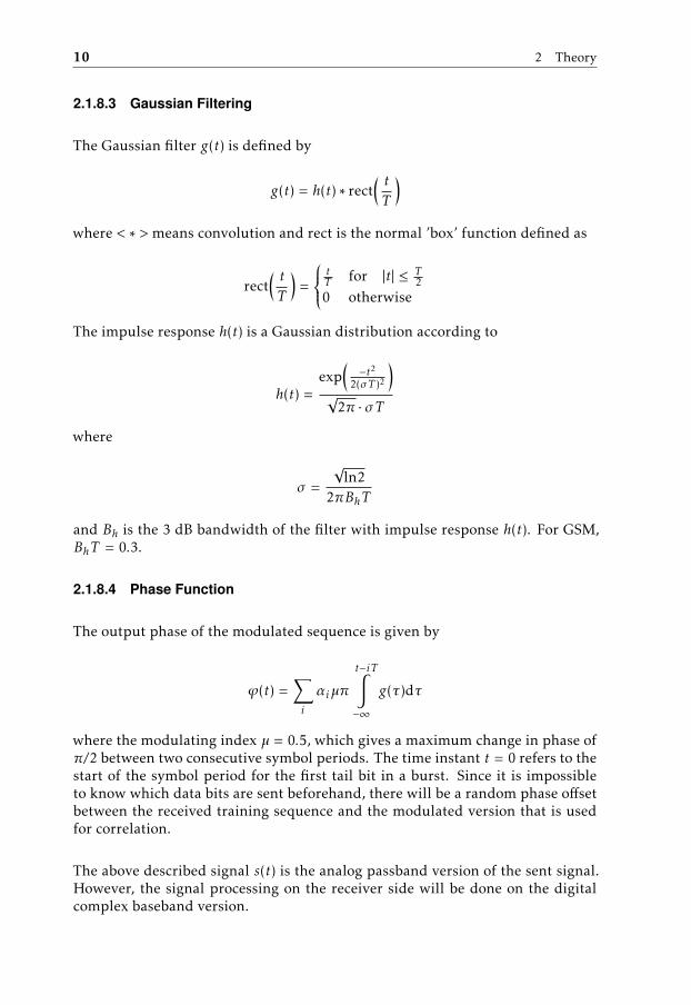
2.1.8.3 Gaussian Filtering

The Gaussian filter g(t) is defined by

g(t) = h(t) ∗ rect( tT

)where < ∗ > means convolution and rect is the normal ’box’ function defined as

rect( tT

)=

tT for |t| ≤ T

20 otherwise

The impulse response h(t) is a Gaussian distribution according to

h(t) =exp

(−t2

2(σT )2

)√

2π · σT

where

σ =

√ln2

2πBhT

and Bh is the 3 dB bandwidth of the filter with impulse response h(t). For GSM,BhT = 0.3.

2.1.8.4 Phase Function

The output phase of the modulated sequence is given by

ϕ(t) =∑i

αiµπ

t−iT∫−∞

g(τ)dτ

where the modulating index µ = 0.5, which gives a maximum change in phase ofπ/2 between two consecutive symbol periods. The time instant t = 0 refers to thestart of the symbol period for the first tail bit in a burst. Since it is impossibleto know which data bits are sent beforehand, there will be a random phase offsetbetween the received training sequence and the modulated version that is usedfor correlation.

The above described signal s(t) is the analog passband version of the sent signal.However, the signal processing on the receiver side will be done on the digitalcomplex baseband version.

2.1 GSM 11

Table 2.2: List of different possible training sequences depending on BCC[3GPP, 2013].

BCC Training Sequence

0 (0,0,1,0,0,1,0,1,1,1,0,0,0,0,1,0,0,0,1,0,0,1,0,1,1,1)1 (0,0,1,0,1,1,0,1,1,1,0,1,1,1,1,0,0,0,1,0,1,1,0,1,1,1)2 (0,1,0,0,0,0,1,1,1,0,1,1,1,0,1,0,0,1,0,0,0,0,1,1,1,0)3 (0,1,0,0,0,1,1,1,1,0,1,1,0,1,0,0,0,1,0,0,0,1,1,1,1,0)4 (0,0,0,1,1,0,1,0,1,1,1,0,0,1,0,0,0,0,0,1,1,0,1,0,1,1)5 (0,1,0,0,1,1,1,0,1,0,1,1,0,0,0,0,0,1,0,0,1,1,1,0,1,0)6 (1,0,1,0,0,1,1,1,1,1,0,1,1,0,0,0,1,0,1,0,0,1,1,1,1,1)7 (1,1,1,0,1,1,1,1,0,0,0,1,0,0,1,0,1,1,1,0,1,1,1,1,0,0)

2.1.9 Relevant Information

Within the data part of the SCH burst (see Figure 2.3), there is some informationwhich can be useful when trying to find the time of arrivals. After demodulationand decoding, one can retrieve the TDMA frame number (FN) and the base sta-tion identity code (BSIC) [3GPP, 2013]. FN tells you which TDMA frame yourSCH burst belongs to (i.e. TS0 in that TDMA frame). This number can be usedto make sure that both receivers correlate with the same training sequence, if thesynchronization error is assumed relatively large.

The BSIC consists of two separate, 3-bit parts: the network color code (NCC) andthe base station color code (BCC). The primary purpose of these color codes is todistinguish between different operators and base stations if they transmit on thesame frequency. However, in this case, the BCC information is used to determinewhich training sequence is used in the normal burst.

2.1.10 Training Sequences

There are eight different training sequences that can be used, depending on oper-ator and base station. These are listed in Table 2.2.

The longer training sequence used in the SCH burst look like:

(1, 0, 1, 1, 1, 0, 0, 1, 0, 1, 1, 0, 0, 0, 1, 0, 0, 0, 0, 0, 0, 1, 0, 0, 0, 0, 0, 0, 1, 1, 1, 1, 0, 0, 1, 0, 1, 1...

...0, 1, 0, 1, 0, 0, 0, 1, 0, 1, 0, 1, 1, 1, 0, 1, 1, 0, 0, 0, 0, 1, 1, 0, 1, 1)

12 2 Theory

2.2 Time-Based Localization

This section gives a detailed view of the localization technique on which thismaster thesis is built upon, called double differential time of arrival (DDTOA).First, some well-known variations are presented, namely TDOA and TOA. Thesetechniques are closely related to DDTOA, and are therefore fit as an introduction.

2.2.1 Time Difference of Arrival

Normal TDOA uses the difference in time of arrival of a signal at two receivers,who are separated by some distance. The absolute time when the signal left thetransmitter is not important, nor the time when the signal arrives at the two re-ceivers. However, the synchronization between the receivers is vital for a correctcalculation of the time difference. In practice, the signal to be located is recordedat both receivers. Then, the two versions are compared with each other to find thetime delay [Arbring and Hedström, 2010]. The received signals can be describedin the following way:

x1(t) = s(t) + w1(t)

x2(t) = s(t + ∆) + w2(t)

x1 is the signal recorded at receiver 1 and x2 the same signal recorded at receiver 2with some delay ∆. w1 and w2 represent addative white Gaussian noise (AWGN).Since the signals are recorded simultaneously, and the receivers being (to some ex-tent) fully synchronized, ∆ can be determined by calculating the cross-correlationfunction rx1x2

.

rx1x2(τ) = E[x1(t)x2(t + τ)] (2.1)

∆ is determined as the τ that maximizes the absolute value of the correlationfunction. The calculations can also be done in the frequency domain, and in thiscase ∆ is found as the gradient of the angle part of the cross spectra Sx1x2

(f ) =

F{rx1x2

(τ)}.

The time difference ∆ is then used together with the constant propagation speedof radio signals to calculate a hyperbola of possible possitions for the origin ofthe signal.

|PMs − P

Rx1| − |PMs − PRx2| = c∆ (2.2)

PRx1, P

Rx2 and PMs represent the positions in Cartesian coordinates of receiver

1, receiver 2 and the mobile, and c the speed of light. Figure 2.5 shows someexamples of hyperbolas for different ∆. The receivers are represented by the largedots in the figure. To get an exact location of the transmitter, at least one more

2.2 Time-Based Localization 13

Figure 2.5: The possible locations (one hyperbola) for the transmitter, for anumber of different values of the time delay ∆. A smaller value of ∆ gives ahyperbola closer to the midpoint between the two receivers.

receiver is needed in order to calculate an intersection point. The position of thereceivers is important in order to get good accuracy, but also to avoid false mirrorlocations as could appear if the receivers are located on a line.

2.2.2 Time of Arrival

TOA1 is a technique that, as the name implies, uses the time instant for which thesignal arrives at the receiver [Gezici et al., 2005]. In this case, synchronization aswell as communication between the receiver and the transmitter is crucial.

The time (∆) it takes for the signal to travel from transmitter to receiver, againtogether with the speed of light, gives the radius (ρ) for a circle of possible loca-tions of the source. Information about when the signal was sent is required inorder to get the propagation time (this is the necessary communication betweentransmitter and receiver). Three or more calculations from different receivers de-termines the exact position, through regular triangulation. See Figure 2.6.

ρ = c∆ (2.3)

1In this case, TOA is refered to both the name of the method, as well as the time of arrival for asignal.

14 2 Theory

���

�1

�2

�3

Figure 2.6: Positioning using TOA. The arrow marks the spot of the transmit-ter Ms.

TOA is a technique that can not be used in an electronic warfare situation (interms of finding enemy forces), due to the fact that communication and synchro-nization between receiver and transmitter is needed. However, it is possible tocalculate the position of the transmitter without the knowledge of when the sig-nal was sent. By comparing the TOA values at the three receivers, the location ofthe transmitter can be found by solving an optimization problem; in contrary tocalculating the intersection point of the three circles. This is known as differentialTOA (DTOA).

2.2.3 Double Differential Time of Arrival

The technique presented and examined in this master thesis is called double dif-ferential time of arrival (DDTOA). The idea with this method is to determine thetime delay ∆ between two receivers, just like in TDOA but without the need forsynchronization. The synchronization is instead done using a reference signal,where the origin of the signal is known. Also, instead of correlating the receivedsignals, the time delays are calculated using the difference between the time ofarrival values, as in DTOA.

Two signals are recorded at the receivers, one from the transmitter to be located,and one from the reference source.

In DDTOA, the double represents the added reference signal examined at eachreceiver to compensate for time synchronization errors. The differential standsfor the difference between two time of arrival values of the same signal at two re-ceivers, unlike normal TDOA which compare the signal recorded at two receivers(Equation 2.1).

The calculations to determine the actual position will be the same as for normalTDOA, it is the method of finding the time difference ∆ that differs. Hence, thereason for only presenting a method to find one hyperbola, on which the user islocated, in this thesis. The rest of the positioning is pure geometry and nothingnew.

2.2 Time-Based Localization 15

���

���

���1 ���2

Figure 2.7: Overview of the system.

2.2.3.1 Calculating the Time Difference

The system setup is again shown in Figure 2.7. PRx1, P

Rx2, PMs and P

Bs repre-sents the positions of receiver 1 and 2, the mobile to be located and the referencesource (base station). The time difference is given as

∆ = τMs,Rx1 − τMs,Rx2 + δ − (τ

Bs,Rx1 − τBs,Rx2) (2.4)

where τx,y is the time of arrival at location y for a signal sent from location x. δ isthe true time difference for a signal traveling from the reference source to receiver1 and 2 respectively. As mentioned in Chapter 1, the positions of receiver 1, 2 andthe reference source are known beforehand, so δ can be determined by geometrycalculations.

The righthand side of equation 2.4 can be divided into two parts:

(τMs,Rx1 − τMs,Rx2)︸ ︷︷ ︸

Time diff. part

+ (δ − (τBs, Rx1 − τBs,Rx2))︸ ︷︷ ︸

Synchronization part (error)

In the case where the receivers are synchronized, the reference source and therebythe synchronization part would not be required. This corresponds to

δ − (τBs, Rx1 − τBs,Rx2) = 0 (2.5)

which of course goes hand in hand with the fact that the calculated reference timedifference should be equal to the predetermined value δ, according to

τBs,Rx1 − τBs,Rx2 = δ (2.6)

16 2 Theory

Equation 2.6 will be used in the field experiment as a verification on how accuratethe measurements are, by using synchronized receivers.

In the aspect of keeping a low profile in war, the communication between friendlyforces must be kept to a minimum. Therefor, the terms in Equation 2.4 are re-ordered according to

∆ = (τMs,Rx1 − τBs,Rx1) − (τ

Ms,Rx2 − τBs,Rx2) + δ (2.7)

In this way, it is possible to subtract the time stamps at a specific receiver beforesending the values to a third party for the ∆-calculation. This comes in handywhen averaging over a larger number of signals for one time difference calcula-tion. An illustrative picture is shown in Figure 2.8.

Synchronization error

� 0 � 8 � 22

�2 0 �2 6

3

�2 29

,

, 2

� ,

� , 2

^ ^

^^

5

t

t2

Time for Rx1

Time for Rx2

Figure 2.8: Example of time stamps. The numbers are given in time units.According to Equation 2.4, the time difference will be ∆ = (22 − 29) + (−3) −(8 − 6) = −7 − 3 − 2 = −12. The sign of ∆ and δ is determined by Rx2 sub-tracted from Rx1.

2.2.3.2 Evaluation of Bound for Synchronization Error

As mentioned in Section 2.1.5, it is the training sequences within the burst thatwill be used for the time stamps. They are sent with some time period TP sepa-rated from each other. TP is approximately 4.6 ms for the uplink communication,and approximately 46.2 ms for downlink communication. To be sure that thetime stamps from the same transmitted training sequence are being compared,the synchronization error εsync needs to be below a certain limit.

2.2 Time-Based Localization 17

To start with, lets assume that

∆� TP and δ � TP

This is a reasonable assumption, since the lower value on TP , 4.6 ms, correspondsto a propagation distance of 1380 km for a radio signal. This is a distance muchlarger than that possible for mobile communication. Using this assumption, thesynchronization error will be bounded by

|εsync| <TP2

Figure 2.9 shows the area for which the synchronization error can drift, withoutthe possibility of comparing two different training sequences.

��

��−1 ��+1 �� ^ ^ ^

Area for

synchronization error

Figure 2.9: Synchronization error.

In the case when the synchronization error is bigger than half the training se-quence repetition period, some kind of extra information about the training se-quence is required. This is where the TDMA frame number (FN) can be used. Thedata part of an SCH burst contains a number specific for the TDMA frame whichthe burst belongs to. This makes it possible to attach a number to each SCH train-ing sequence, and in this way make sure that the same training sequence is usedfor the time stamp at both receivers, regardless of how large the synchronizationerror is.

To make sure that the same training sequences are used for the uplink commu-nication, the synchronization error is first calculated and then compensated for.After this, it is possible to pair two matching uplink training sequences and cal-culate the time difference ∆. In this case, the advantage gained from Equation 2.7is lost, since both TOA values needs to be sent to the third party instead of onlythe difference between the values.

3Method

This chapter describes the method used to implement the theory from Section2.2.

3.1 Correlation

To determine the time stamps for which the signals arrives at the receivers, corre-lation is used. How good two signals correlate with each other can be seen as ameasurement on how closely related they are to each other. The recorded signalsare therefore correlated with the known training sequences. The highest values(i.e. the peaks) in this correlation function should thereby point out where thereceived training sequences are located within the recorded signals. The timestamps for these peak values are then used as the time of arrival for the signal.See Figure 3.1 and 3.2.

Cross

Correlation

Peak

Detection

Received Signal

Known Training Sequence

Arrival Time

Figure 3.1: Cross correlation between the received signal and the knowntraining sequence, together with peak detection, gives the time of arrivalvalue.

19

20 3 Method

Figure 3.2: Correlation peak gives the time of arrival value.

3.1.1 Mathematical Description

To get a better understanding of why this works, we use the squared Euclideandistance between two signals [Larsson, 2012], for example y1(t) and y2(t). TheEuclidean distance is zero only if y1(t) = y2(t) for all t1. Hence, the shorter thesquared Euclidean distance is, the more similar the signals are.

A simple model of the system is

x(t) = s(t − τ) + w(t)

where x(t) is the received signal which is described as a time delayed version ofthe sent signal s(t) with some added noise w(t). Determine time of arrival willcorrespond to finding the time delay, if the receiver knows the time the signalwas sent. Note that this is only true if transmitter and receiver are synchronized,which they are not in this case. However, the actual propagation time delay is notof interest here, only the differential time delay between two receivers.

Without the influence of noise, x(t) and s(t − τ) would be equal, and the squaredEuclidean distance zero. Thus, minimizing the squared Euclidean distance be-tween x(t) and s(t − τ) should give the best approximation of the time delay. Thiscan be mathematically described as

1With some restrictions on the signals

3.1 Correlation 21

∞∫−∞

(x(t) − s(t − τ)

)2dt =

∞∫−∞

(x2(t) + s2(t − τ) − 2x(t)s(t − τ)

)dt (3.1)

=

∞∫−∞

x2(t)dt +

∞∫−∞

s2(t − τ)dt − 2

∞∫−∞

x(t)s(t − τ)dt

=

∞∫−∞

x2(t)dt +

∞∫−∞

s2(t)dt − 2

∞∫−∞

x(t)s(t − τ)dt

In this way it is possible to see that minimizing the squared Euclidean distance isthe same as maximizing the expression

rx,s(τ) =

∞∫−∞

x(t)s(t − τ)dt =

∞∫−∞

x(t + τ)s(t)dt (3.2)

with respect to the time delay τ . We now formulate the formal definition of(deterministic) cross correlation between two, possibly complex, signals:

3.1 Definition. Cross Correlation

ry1y2(τ) =

∞∫−∞

y∗1(t)y2(t + τ)dt

where < ∗ > denotes complex conjugate.

The τ-value which gives the highest value of |rx,s(τ)| will be the estimated time ofarrival (τ) for the training sequence.

To summarize, the received signal is correlated with the known training sequence.The parts in the received signal where the training sequence is located shouldgive the highest values for the correlation function, according to Equation 3.1(they are likely most similar, so the euclidean distance is minimized). The timestamp for these peak values are used as the time of arrivals. In this way, it ispossible for two receivers to compare time of arrivals of the same transmittedtraining sequence. The added noise can be seen as a way of distorting the peaks.

In reality, there exists no infinitely long signals. The practical aspects of imple-menting the correlation function will be given later in this chapter.

22 3 Method

3.1.2 Comments on Accuracy

How accurate the calculation of the time stamp can be, comes down to essen-tially three different things: how high the signal to noise ratio (SNR) is, how longthe overlapping correlation sequence is (meaning, the length of the training se-quence, L) and also how much bandwidth (B) the transmitted signal occupies?The first thing is easy to get a grip on. The higher the noise levels are, the more af-fected by the noise will the received training sequence be. This will influence thesimilarity between the received training sequence and the real one that is usedfor correlation, and there by the sharpness of the peak. If the noise is too high, itcould even be impossible to distinguish the peak from the rest of the correlateddata.

The reaction on the peak due to longer or shorter training sequences is also quiteintuitive. The more unique information you have available, the more reliablewill the outcome be, whatever it is. A longer training sequence should thereforegive a better estimation of the time of arrival. As seen in Chapter 2, the twoavailable types of training sequences are 26 respectively 64 bits long. In mobilecommunication, these are used for detection and demodulation, as a way of es-timating the channel. The shorter one is used in a burst whose main purposeis to transmit data, while the longer one is used in a burst for synchronization.There is of course always a trade-off between good channel estimation and highdata throughput. The 64 bits sequence will be used for the signals sent fromthe base station since these bursts are broadcast. The 26 bits sequence will beused for the signals transmitted from the mobile station. Hence, the accuracy ofthe TOA from the base station should be better than the one from the mobile. Itshould also be noted that the training sequences are designed to have good autocorrelation properties, i.e. high peaks.

The connection between available bandwidth and the sharpness of the correla-tion peak is perhaps not as intuitive. Approximately, the width of the peak isinversely proportional to the bandwidth of the signal [Larsson, 2012]. This isdue to the uncertainty principle of the Fourier transform. The idea of this prin-ciple states that is impossible for a signal to have all its energy within a certaintime interval, and at the same time only occupy a limited number of frequencies[Du]. One way to exemplify this is to consider the Fourier transform of the sincfunction, which is a rectangular function:

y(t) = sinc(at)→ F{y(t)

}=

1/a if |f | ≤ a/20 if |f | > a/2

A higher value of a provides a more narrow peak in the time domain, but a widerbox in the frequency domain. This implies that the more bandwidth you haveavailable, the more accurate will the calculation of the time of arrival be. Also,the energy should be spread out as evenly as possible over the bandwidth. Ameasure of this is known as the effective bandwidth.

3.2 Curve Fitting 23

L and B are predefined values of the GSM standard, and thereby constant in thiscase. The SNR is hard to influence, apart from choosing a good receiver positionrelative to the base station and using a good antenna high above the ground. How-ever, there is one thing that can increase the accuracy of the calculations; namelythe use of sample interpolation.

3.2 Curve Fitting

Sample interpolation, or curve fitting, is a method which estimates a larger num-ber of function values given a smaller, discrete set of values. In this case, thecorrelation peaks will be approximated by a polynomial of the second order. In-stead of only letting the maximum value of the peak represent the position forthe time of arrival, several neighbouring samples are interpolated to a second de-gree curve. The zero-root of the derivative of this curve is then used as the timestamp. See Figure 3.3.

3.3 Averaging

Since one single phone call includes a large number of training sequences (M), itis possible to decrease the estimation error by averaging over several TOA mea-surements. This gives

∆ =1M

M∑i=1

τMs,Rx1[i] − τ

Ms,Rx2[i] + δ − (τBs,Rx1[i] − τ

Bs,Rx2[i]) (3.3)

where τ[i] is a vector containing M different TOA values from one telephone call.

3.4 Implementation

All of the implementation has been done in Matlab.

3.4.1 Demodulation and Frequency Correction

Demodulating and decoding the downlink broadcast signals is a field big enoughto be a master thesis of its own. It includes subjects as time synchronization,frequency correction, equalization, demodulating symbols into bits and decodingthe raw data bits into readable information. Therefore, the theory behind thispart is left out of this report. For the interested, [Pathak] and [Bapat et al., 2005]are suggested. Frequency correction is sometimes needed because of receiverhardware limitations (unstabilized oscillators).

The code used for the demodulation as well as the frequency correction in theimplementation has been taken from [Ekstrøm and Mikkelsen, 1997].

24 3 Method

−2.5 −2 −1.5 −1 −0.5 0 0.5 1 1.5 2 2.5−3

−2

−1

0

1

2

3

4

5

t

y(t)

Figure 3.3: The figure shows the function y(t) = −t2 + 2, and ’*’ marks theavailable samples around the peak (t = 0). By only using the maximum value,the time of arrival would be -0,2. However, by interpolating the samples as asecond degree curve, and calculate an estimate of the value t where y′(t) = 0,the time of arrival will become approximately 0 (using Matlab’s functionpolyfit).

3.4.2 Practical Aspects

When talking into a mobile phone, the amplitude of the signal goes up and downdepending on when you are speaking and when you are silent between the words.Because of this, some graphical observations of the correlation plots were done,to chose the part of the signal with the highest amplitude.

3.4.3 Discrete Correlation

For the discrete implementation of the cross correlation function, Matlab’s xcorrwas used [Mathworks, 2013]. It estimates the true value as

3.4 Implementation 25

ry1y2[n] =

N−n−1∑m=0

y1[m + n]y∗2[m] for n = 0, ..., N − 1

r∗y2y1[−n] for n = −(N − 1), ...,−1

where N is the number of samples for the longer signal (i.e. the received signal).

3.4.4 Interpolation

The interpolation was implemented using Matlab’s function polyfit, and thecalculation of the zero-root of the derivative by using polyder followed by roots.

3.4.5 Modulated Training Sequence

To get a better understanding of how to implement the modulated baseband ver-sions of the training sequences, a different expression for the frequency functiong(t) was derived.

The frequency function g(t) can be approximated as a Guassian distribution ac-cording to

g(t) = h(t) ∗ rect( tT

)(3.4)

=1

√2πσT

∞∫−∞

exp( −τ2

2(σT )2

)rect

( t − τT

)dτ

=/− T

2≤ t − τ ≤ T

2⇒ τ ≥ t − T

2andτ ≤ t +

T2

/

=1T

1√

2πσT

t+T /2∫t−T /2

exp( −τ2

2(σT )2

)dτ

=1T

1√

2πσT

∞∫t−T /2

exp( −τ2

2(σT )2

)dτ −

∞∫t+T /2

exp( −τ2

2(σT )2

)dτ

=

1T

Q( t − T /2σT

)− Q

( t + T /2σT

)≈ 1T

T 1√

2πσ2exp

( −t22σ2

2

) =1

√2πσ2

exp( −t2

2σ22

)Note that the last row in the expression is only an approximation, where σ2 =1.957002 · 10−6. This gives the following appearance of the phase function ϕ(t):

26 3 Method

ϕ(t) =∑i

αiµπ

t−iT∫−∞

1√

2πσ2exp

(−τ2

2σ22

)dτ (3.5)

=∑i

αiµπ

∞∫−∞

1√

2πσ2exp

(−τ2

2σ22

)dτ −

∞∫t−iT

1√

2πσ2exp

(−τ2

2σ22

)dτ

=

∑i

αiµπ

1 − Q( t − iTσ2

)To get the discrete values of the phase function, ϕ(t) is sampled for t = nT , withsome possible oversampling:

ϕ[n] = ϕ(t =nTΛ

) for n = 1, 2, 3, ..., L ·Λ (3.6)

where L is the number of modulated symbols and Λ the oversampling rate. Thebaseband representation of the modulated training sequence can then be imple-mented as

xTR

[n] = eϕ[n] (3.7)

3.4.6 Algorithms

Figures 3.4 - 3.7 show block diagrams over the implementation algorithms, in cor-rect sequence of execution order. They give a rough description on the differentsteps and the input and output parameters.

fOFFSET

BCC

FN

Demodulationx[n]

Figure 3.4: The received downlink signal is first demodulated to retrieve thefrequency offset foffset, the BCC and the FN. Finding the frequency offset isseen as a part of the demodulation process.

3.4 Implementation 27

Modulation

Training Sequence

Bits

BCC

xTR[n]

Figure 3.5: Modulation of the training sequences. Input is bits and output isthe complex baseband representation. BCC is used when modulating the 26bit sequence (uplink).

x[n]

xTR[n]

fOFFSET

Frequency

CorrectionFind

Approximate

Position

Cross

Correlation

Peak

Detection

FN

�k^

Figure 3.6: Block digram showing the algorithm to find the TOA for thereceived signal. The process is iterated over the number of available corre-lation peaks (M) in the signal. FN is used for the downlink signal, to pin aspecific number to the TOA value.

SubtractionSubtraction

Subtraction

Addition

Mean

τRx1,Bs^

τRx2,Bs^

τRx1,Ms^

τRx2,Ms^

Figure 3.7: Block diagram showing the calculations of ∆, given the true timedelay δ and the TOA values as input. The result is averaged over the availablenumber of peaks (M).

4Simulation

Simulations were done in order to test the method. It should be noted that themodel used for the simulations is quite simple. It doesn’t say much about the realcase, since difficulties like for example multipath propagation is avoided. Also,the available size of the bandwidth is neglected. However, it is a good way oftesting the correlation and interpolation, with respect to SNR and the length ofthe training sequence.

4.1 System Model

The positions for the nodes in the simulation model can be seen in Figure 4.1. Theimaginary receivers, base station and mobile station are placed in the corners ofa square. Hence, both ∆ and δ are equal to zero.

The signals used in the model are the modulated baseband version of the knowntraining sequences, together with the imaginary received signal created as thetraining sequence with added white gaussian noise.

xtr[n] Modulated training sequence

x[n] = xtr[n] + w[n] Training sequence with added noise

4.2 Calculations

The idea is to first get an estimation of the error of the TOA values by correlatingthe modulated training sequence with the noisy version, determine the locationof the peak value by interpolation, and finally comparing it with the expected

29

30 4 Simulation

���

���

���1

���2

Figure 4.1: The hypothetical locations in the simulation model. Both ∆ andδ are equal to zero due to the symmetry between the four nodes.

value zero. See Figure 4.2. Correlation between the two signals without addingnoise gives the auto correlation function for the training sequence, which in the-ory is symmetric around zero. Hence, comparing the TOA estimate with respectto the zero value shows how the peak detection is influenced by the noise.

The TOA error, τerror, is then used to calculate the root mean square error (RMS)of the estimation, according to

εtoa =

√√√√1

Nest

Nest∑j=1

(τerror[j]

)2(4.1)

Nest = 1000 is the number of estimated TOA errors. By doing this for a number ofdifferent values on the noise energy and for both training sequences, it is possibleto compare RMS with respect to SNR and signal length.

The RMS values from the TOA estimation are then used in Equation 3.3 to get arelationship between SNR and the RMS for the time delay ∆. A single value ofthe DDTOA error, ∆error, is estimated as

xTR[n]

x [n]~

�ERROR

^

Cross

Correlation

Peak

Detection

Figure 4.2: Correlation between the two signals used in the model, followedby peak detection gives the error of the TOA estimate.

4.3 Results 31

∆error =1M

M∑i=1

χul[i] − ξul[i] − (χdl[i] − ξdl[i]

) (4.2)

where the TOA values are implemented as normally distributed variables withzero mean and a standard deviation equal to the RMS from the TOA estimation:

χul, ξul ∼ N (0, εtoa,ul)

χdl, ξdl ∼ N (0, εtoa,dl)

The subscripts ul and dl indicates downlink and uplink communication. Equa-tion 4.2 gives an estimation of the DDTOA error since the true values of ∆ andδ in the model are both equal to zero. The RMS of the DDTOA estimation canfinally be calculated according to

εddtoa =

√√√√1

Nest

Nest∑j=1

(∆error[j]

)2(4.3)

4.3 Results

First, the RMS value for a TOA estimation were calculated without adding anynoise, to see that the location of the peak actually is zero. This gives

εtoa = 2.245 · 10−22 s

which in this case very well can be approximated with zero. The sampling fre-quency, i.e. the inverse of the time between two samples, used in the model isthe same as in the laboratory trials and is equal to 4’333’328 Hz (the symbol rateoversampled by 16).

Figures 4.3 and 4.4a show the correlation functions for the 64 bit and the 26 bittraining sequences respectively, while Figure 4.4b shows a zoomed in version of4.4a. In the latter, it is possible to see how the noise affects the location of thecorrelation peak.

32 4 Simulation

−2 −1.5 −1 −0.5 0 0.5 1 1.5 2 2.5

x 10−4

0.1

0.2

0.3

0.4

0.5

0.6

0.7

0.8

0.9

1

Time [s]

Abs

olut

e va

lue

of th

e co

rrel

atio

n fu

nctio

n

Figure 4.3: Plot of the (normalized) correlation function for the 64 bit train-ing sequence, without noise. The function is symmetric around zero.

4.3 Results 33

−1 −0.8 −0.6 −0.4 −0.2 0 0.2 0.4 0.6 0.8 1

x 10−4

0

0.1

0.2

0.3

0.4

0.5

0.6

0.7

0.8

0.9

1

Time [s]

Abs

olut

e va

lue

of th

e co

rrel

atio

n fu

nctio

n

SNR = −5 dBzero valueno noise

(a) Correlation function

−4 −3 −2 −1 0 1 2 3 4 5

x 10−6

0.2

0.3

0.4

0.5

0.6

0.7

0.8

Time [s]

Abs

olut

e va

lue

of th

e co

rrel

atio

n fu

nctio

n

SNR = −5 dBzero valueno noise

(b) Zoom in

Figure 4.4: (a) Plot of the (normalized) correlation function for the 26 bittraining sequence (BCC = 1). Both without the impact of noise and withadded noise (SNR = -5 dB). (b) Zoom in on the correlation function. Thepeak is located some what to the right of the zero value, due to the influenceof the noise.

34 4 Simulation

The RMS from the TOA estimations can be found in Figure 4.5. The figure clearlyshows how the error decreases as the SNR increases, and also that the longertraining sequence gives better results than the shorter one. All according to theargumentation on accuracy in Chapter 3.

Figure 4.6 shows the result of the DDTOA estimation. This time, the RMS ismultiplied by c to get the error in meters instead of seconds. Simulations wheredone using different values onM for the averaging. The plot shows that averagingcan be very useful when the SNR is low, but of less importance when the SNR ishigh.

The RMS value connected to a specific SNR in Figure 4.5 were used in the calcu-lation of the RMS value in Figure 4.6, connected to the same SNR.

It should be noted that the error values presented here are not the distance errorfrom the actual mobile station position, but the error from one ∆ calculationbetween two receivers, at the baseline (the line intersecting with both receivers).

−5 0 5 10 15 20 2510

−9

10−8

10−7

10−6

RM

S [s

]

SNR [dB]

64 bit training sequence26 bit training sequence

Figure 4.5: Plot showing the RMS due to the impact of noise.

4.3 Results 35

−5 0 5 10 15 20 250

10

20

30

40

50

60

70

80

90

100

RM

S [m

]

SNR [dB]

M = 1M = 10M = 100

Figure 4.6: The RMS for the estimation of ∆, when averaging over 1, 10 and100 of each TOA value.

5Laboratory Trials and Field Test

This chapter describes the trials that have been done to examine the DDTOAsystem, along with their results. Experiments were made in both a laboratory andin a field test. In the laboratory, the two receivers Rx1 and Rx2 were connectedto the same antenna, meaning, the receivers are located at the same position. Nolocalization of the mobile signal is possible in this case, since the time delay ∆

always will be zero, no matter where the mobile station is located. However, itis possible to test the implementation and the accuracy of the calculations. Sinceboth ∆ and δ is zero in this case, you can calculate the time delay for a phone call,compensate for the synchronization error with the help from a reference signaland then compare it to the zero value. This provide an indication of the errormargin for the system.

For the field experiment, one of the receivers was put in a car and driven awayfrom the laboratory. This setup made it possible to test the system in an actualpositioning situation.

First, the equipment is described, then the system setups and finally the resultsof the trials.

5.1 Receiver Hardware

A block diagram of the receiver can be seen in Figure 5.1. In short, it is madeof an antenna, a tuner, an A/D-converter, a DDC (digital down converter) and astorage system. The tuner moves the RF (radio frequency) signal from the 900MHz band down to an IF (intermediate frequency) signal centered around 10.7MHz. The A/D-converter together with the DDC converts the analog signal to adigital baseband signal (I/Q data) and stores it on a file. The DDC has multiple

37

38 5 Laboratory Trials and Field Test

Tuner

A/D

DDCRF IF I/Q

Storage

Figure 5.1: Components of the receiver. The tuner is a Rohde&SchwarzEB200 Miniport Receiver, and the A/D-DDC system is manufactured byPentek, Inc. (Model 7152) and programmed by FOI staff.

inputs making it possible to record the signal from the mobile and the signalfrom the base station at the same time.

5.2 TEMS Mobile Phone

In order to simplify the experiments, a special kind of mobile phone was used. Ithas an operation mode called TEMS (test mobile system), which makes it possi-ble to choose between GSM and 3G, see the available frequency cells (channels)and also to force the mobile to transmit and receive on a particular channel. Inthis way, the receivers can tune in on the correct frequency from the beginning,instead of searching through the entire frequency band. Since these trials are notmade in real time, searching for the mobile signal is not even an option. Further,one can be sure that it is the signal from the correct mobile that is being local-ized. If more than one mobile should use the same frequency channel, it will benoticed since more than one time slot will be occupied.

5.3 Execution

A phone call made from the TEMS mobile was recorded using the receivers. Therecording time was set to 6 s (longer recording time is possible but creates prob-lems with large data files). The downlink frequency Fd was set to 952.4 MHz,corresponding to channel 87. The analog signal is sampled with a frequency of160 MHz. After the signal processing in the DDC, the signal is downsampled to5 MHz, to extract unnecessary information and reduce the size of the file. Finally,the digital signals are reshaped in Matlab to a sample frequency Fs = 4’333’328Hz, to match an oversampling of the symbol rate by 16 (for simplicity, the over-sampling should be a multiple of 4, since the guard periods in the bursts have aduration of 8.25 bits).

To induce a synchronization error within the system, one receiver (Rx1) was run-ning with a GPS clock reference, while the other (Rx2) used a floating clock ref-erence. This setup created a synchronization error between 0 and 1 s. A detailedblock diagram of the links and wires can be found in Figure 5.2. Two EB200

5.3 Execution 39

32

32

DD

CD

DC

EB

20

0E

B2

00

10 M

Hz

(GP

S)

1 P

PS

(GP

S)

160 M

Hz

RE

FR

EF

RE

F

32

32

DD

CD

DC

EB

200

EB

200

10

MH

z

(Flo

ating)

1 P

PS

(Flo

ating)

16

0 M

Hz

RE

FR

EF

RE

F

Rx

1R

x2

Figure 5.2: A detailed view of how the components in the receivers are con-nected, in the case for the laboratory trials. For the field experiment, thesetup was the same, except for the receivers having their own antenna. Thetuners, as well as the 160 MHz signal generator, uses a 10 MHz clock ref-erence as a stabilizer. The 1 PPS (pulse per second) is used to trigger therecording. Since Rx1 uses a GPS as reference while Rx2 uses a floating refer-ence, the recordings are triggered at different times within the same second,creating a synchronization error between 0 and 1 s.

40 5 Laboratory Trials and Field Test

tuners were used together with each receiver; one tuned in on the downlink fre-quency and the other on the uplink frequency.

Some attempts were also made using a GPS reference in both receivers, to see ifthere would be any difference in the performance.

5.3.1 Laboratory Setup

For the laboratory trials, the two receivers were connected to the same antenna,which was placed on the roof of the building. Figure 5.3 shows the positions forthe four object. Two different locations were tested for the mobile, one close tothe antenna (to provide better SNR) and one further a way.

Bs

Rx1, Rx2

A B

Figure 5.3: Positions for the laboratory trials. a and b marks the spots forthe mobile stations. The antenna connected to the two receivers is located onthe roof of the laboratory. The area is located south of Linköping University,Linköping, Sweden.

As mentioned before, the true values on ∆ and δ in this case are both zero. Table

5.3 Execution 41

Table 5.1: Parameters for the laboratory attempts. Fu is the uplink fre-quency.

Attempt Position Fu [MHz] BCC

i B 907.4 1ii B 913 5iii A 907.4 1

5.1 shows the parameters for the attempts using the laboratory setup.

5.3.2 Field Test Setup

Figure 5.4 shows the positions for the field test. The location for the mobile sta-tion was chosen to give approximately the same distance to both receivers, andin this way provide equal signal strength at both receivers. The true values on∆ and δ was determined using the GPS coordinates for the objects, convertingthem to RT90 (Rikets nät or Swedish grid ) coordinates followed by geometricalcalculations of the distances between the objects. Rx2 had a large bias due to along cable between the antenna and the tuner. However, this bias is the same for∆ and δ, so it will not effect the result.

Table 5.2 below gives the parameters for the attempts in the field test.

Table 5.2: Parameters for the attempts in the field experiments.

Attempt Fu [MHz] BCC

iv 909.4 7v 909.4 7vi 909.4 7vii 909.4 7viii 907.4 1ix 907.4 1

42 5 Laboratory Trials and Field Test

Bs

Rx2

Ms

Rx1

Figure 5.4: Positions for the field experiment. The position for the mobilestation (Ms) is approximately the same as the one used for the laboratorytrials (b).

5.4 Results 43

5.4 Results

5.4.1 Received Signals

First, two examples of received signals are shown to illustrate the difference be-tween the laboratory results and the field experiment results. Figure 5.5 showsthe received uplink signals from Attempt i. In this case, the recorded signals lookthe same in terms of amplitude variations. It is possible to get a rough estimationof the synchronization error just by looking at the plot.

Figure 5.6 shows the received uplink signals from Attempt iv. The signal recordedat Rx1 is a little bit stronger than the one recorded at Rx2, and the amplitude vari-ations are not the same.

5.4.2 Laboratory Trials

The results of the calculation of ∆error from Attempt i, ii and iii can be seenin Figures 5.7, 5.8 and 5.9. The results are given in meters after multiplyingthe time delay with the speed of light. The histograms shows how the values of∆error are distributed. All attempts gave quite good results, as the figures show.The three distributions are centered around zero, with most of the values close tothe true value and a few less accurate. The sign of the error is determined by Rx2subtracted from Rx1.

The outcome after averaging can be found in Table 5.3. When calculating themean value of ∆error, the error is below 1 m in all three attempts.

Figures 5.10 and 5.11 shows the calculated differences between the TOA values,for downlink and uplink respectively. In these plots, it is possible to see how thesynchronization error drift in time due to the floating time reference. They alsoshow that the accuracy from the downlink signal seems somewhat better thanthat of the uplink signal. Finally, both signals indicates the same synchronizationerror, as they should since both ∆ and δ are zero.

Table 5.3: Results from the laboratory trials. M is the number of peaks usedfor TOA calculations during the call (the number used for averaging).

Attempt M (Uplink) M (Downlink) ∆error [m] Synchronization

i 169 100 -0.77 Noii 75 74 +0.78 Noiii 1000 120 -0.94 Yes

44 5 Laboratory Trials and Field Test

0 1 2 3 4 5 60

1

x 10−4

Time [s]

Abs

olut

e va

lue

of I/

Q−

data

0 1 2 3 4 5 60

1

x 10−4

Time [s]

Abs

olut

e va

lue

of I/

Q−

data

Figure 5.5: Absolute value of the received uplink signals from Attempt i.The upper signal is from receiver 1, and the lower from receiver 2. It ispossible to see how the amplitude variates in time. Due to this, only thepart from approximately 3 - 4.5 s were used to calculate the TOA values.Compare with Figure 5.10.

0 1 2 3 4 5 60

2

4

6

8x 10

−4

Time [s]

Abs

olut

e va

lue

of I/

Q−

data

0 1 2 3 4 5 60

1

x 10−4

Time [s]

Abs

olut

e va

lue

of I/

Q−

data

Figure 5.6: Absolute value of the received uplink signals from Attempt iv.The upper signal is from receiver 1, and the lower from receiver 2.

5.4 Results 45

−100 −50 0 50 100 1500

5

10

15

20

25

30

35

40

Delta Error [m]

Num

ber

of D

elta

Err

ors

Figure 5.7: Histogram over the ∆error values for Attempt i. The values of∆error are multiplied by c to get the results in meters. The mean value is-0.77 m after averaging. The correct value is zero (no error).

−300 −200 −100 0 100 200 3000

2

4

6

8

10

12

Delta Error [m]

Num

ber

of D

elta

Err

ors

Figure 5.8: Histogram over the ∆error values for Attempt ii. The mean valueis 0.78 m.

46 5 Laboratory Trials and Field Test

−300 −250 −200 −150 −100 −50 0 50 100 150 2000

50

100

150

200

250

Delta [m]

Num

ber

of D

elta

Val

ues

Figure 5.9: Histogram over the ∆error values for Attempt iii. The meanvalue is -0.94 m.

0 0.5 1 1.5 2 2.5 3 3.5 4 4.5 50.3099

0.3099

0.3099

0.3099

0.3099

0.3099

0.3099

0.3099

0.3099

0.3099

Time [s]

TO

A D

iffer

ence

s [s

]

UplinkDownlink

Figure 5.10: The TOA differences for Attempt i. The uplink signal is thesignal from the mobile, and the downlink signal is the signal from the basestation. As can be seen in the figure, the synchronization error drift in time.Due to this fact, the synchronization error was interpolated as a first orderpolynomial, instead of the normal averaging.

5.4 Results 47

0 0.5 1 1.5 2 2.5 3 3.50.2538

0.2538

0.2538

0.2538

0.2538

0.2538

Time [s]

TO

A D

iffer

ence

[s]

DownlinkUplink

Figure 5.11: The TOA differences for Attempt ii.

5.4.3 Field Test

The results of the calculation of ∆ from the field experiments can be found inFigures 5.13-5.18, in the end of this chapter. The results are given in meters aftermultiplying the time delay with the speed of light. These figures also show howthe values of ∆ are distributed during one phone call (attempt). The true valueof ∆ was calculated to -59 m (Rx1 - Rx2). Table 5.4 shows the outcome afteraveraging.

Table 5.4: Results from the field experiments. The number of training se-quences (M) used in one attempt depends on the appearance of the signal;only the parts with high amplitude (relative the noise) were used.

Attempt M (Uplink) M (Downlink) ∆ [m] ∆errror [m] Synchronization

iv 650 93 -70 -11 Nov 620 117 -140 -81 Novi 525 120 -169 -110 Yesvii 75 120 -100 -41 Yesviii 200 110 -256 -197 Noix 125 110 -120 -61 No

48 5 Laboratory Trials and Field Test

0 100 200 300 400 500 600 700−9

−8

−7

−6

−5

−4

−3

−2

−1x 10

−7

Delta Number

Del

ta [s

]

Figure 5.12: The ∆ values from Attempt v. The values seem to oscillateoutside the variation in accuracy. The part used for the calculations is about3 s long.

5.4.4 Comments on Results

There is a lot of things that can be said about the results from the laboratory trialsand the field test. Yet, it is hard to draw any good conclusions from the outcome.To start with, the results from the trials that were made in the laboratory are quitegood; all of the attempts have an error below 1 meter. This is perhaps even betterthan expected, given the available bandwidth that GSM signals provide and thecomments on accuracy from Section 3.1.2. However, there are single error valuesthat are larger than 200 m. Without the averaging over several ∆-calculationsfrom the same phone call, the result would in most cases be poor.

On the other hand, the outcome of the field experiments was not as good. Bylooking at the histograms from Attempt iv-ix, the error distribution seems tobe quite similar to that of Attempt ii (ranging from about -150 m to +150 m),but unfortunately not centered around the correct value. This could have beenexplained by a bias in the calculations or in the equipment setup, if it wasn’tfor the fact that the bias differs from one attempt to another. It was also notedduring the calculations that the result differs within one attempt depending onwhich part of the signal that was used1.

Figure 5.12 shows an example of how the ∆ values oscillates during one phonecall. The values are from Attempt v.

What this floating bias depends on is hard to say. The first thing that comes tomind is multipath propagation, since it is one thing that clearly differs between

1It should be noted that the results shown in the previous chapter are not chosen as the best ones.The part of the signal with the highest correlation peaks was always chosen for the calculations, nomatter the outcome.

5.4 Results 49

the laboratory trials and the field test. In the first case, since both receivers areconnected to the same antenna, the effect of multiple paths is the same for bothreceivers. This means that the error caused by this phenomena will be avoidedby the differential calculation of TOA values. In the latter case though, the ra-dio waves from the mobile station can take different paths when traveling to thereceivers. However, this error should be rather constant, but perhaps the smallwavelengths and the strong winds (> 10 m/s) during the field test can cause thesefluctuations.

−250 −200 −150 −100 −50 0 50 100 1500

10

20

30

40

50

60

70

80

90

100

Delta [m]

Num

ber

of D

elta

Val

ues

Figure 5.13: Histogram over the ∆ values from Attempt iv. The mean valueis -70 m. The correct value is -59 m. The sum of the bars is the number oftraining sequences (M, uplink) used for averaging, in this case 650. Comparewith Table 5.4.

50 5 Laboratory Trials and Field Test

−300 −250 −200 −150 −100 −500

10

20

30

40

50

60

70

80

90

Delta [m]

Num

ber

of D

elta

Val

ues

Figure 5.14: Histogram over the ∆ values from Attempt v. The mean valueis -140 m.

−350 −300 −250 −200 −150 −100 −500

10

20

30

40

50

60

70

80

90

100

Delta [m]

Num

ber

of D

elta

Val

ues

Figure 5.15: Histogram over the ∆ values from Attempt vi. The mean valueis -169 m.

5.4 Results 51

−200 −150 −100 −50 0 500

2

4

6

8

10

12

14

Delta [m]

Num

ber

of D

elta

Val

ues

Figure 5.16: Histogram over the ∆ values from Attempt vii. The mean valueis -100 m.

−400 −350 −300 −250 −200 −150 −1000

5

10

15

20

25

Delta [m]

Num

ber

of D

elta

Val

ues

Figure 5.17: Histogram over the ∆ values from Attempt viii. The mean valueis -256 m.

52 5 Laboratory Trials and Field Test

−250 −200 −150 −100 −50 0 50 1000

2

4

6

8

10

12

14

16

18

20

Delta [m]

Num

ber

of D

elta

Val

ues

Figure 5.18: Histogram over the ∆ values from Attempt ix. The mean valueis -120 m.

6Conclusions

This chapter summarizes the work and gives some suggestions on future work.

6.1 Results

The final conclusion of the results is that it will be difficult to locate the mobilestation using the current state of the implementation. Still, there is some poten-tial in the possibilities of averaging over large number of training sequences fora single calculation. More research needs to be done to find out what is causingthe big errors, before anything concrete can be said about the accuracy of themethod.

6.2 Suggested Improvements

The first step in the improvements would be to find out what causes the floatingbias. To be able to do this, more efficient algorithms for analyzing the data shouldbe developed. At this stage, it is to much manual work, giving long calculationtimes. This makes it hard to evaluate large amounts of data. Also, more robustequipment can be used, e.g. directional antennas. The location of the base stationis always known, so it is possible to aim the antenna at its direction. This willimprove the SNR. To overcome the problems due to multipath propagation, thereare various methods of super-resolution techniques that could be worth lookinginto.

53

54 6 Conclusions

6.3 Future Developments

To further investigate in the possibilities of DDTOA, there are a lot of other sig-nals of opportunity that can be used for synchronization. For example, radioAM-signals or wireless television signals. Another idea could be to create yourown reference signal. In this way, it is possible to use long training sequenceswith good auto-correlation properties. The drawback of this method would bethe need of an additional object in the system, and also the extra "unnatural"communication that can be detected by the opponent.

A variation of the method could be to only use the synchronization part of theequation, since the reference signals are generally stronger and easier to handlethan those from the cell phone. When the synchronization error is found, it canbe used together with the technique for normal TDOA.

6.4 Final Comments

During the field experiment, some additional positions were tested, further awayfrom the receivers. The signals from these locations were in most cases very weak.A problem with the mobile phone is its power control. Since the reception to thebase station is very good, the mobile lowers the power for transmitting, makingit hard for the receivers to detect the signals (the base station uses much biggerantennas with more gain than the ones used in the field test). The idea fromthe beginning was to compare the stronger signals with the weaker, too see ifthere would be any difference in performance. However, since the outcome fromthe strong signals were poor, the result from the weak signals were only brieflyexamined and excluded from the report.

The starting point for this thesis was the problems with synchronizing receiversin a positioning system. Normal TDOA is dependent on GPS signals, so the ideawas to create a system that could be used if the connection to the satellites is lost.In retrospect, the focus should perhaps have been more towards the synchroniza-tion part of this method, and less on the actual positioning. In this way, maybethe outcome would have been more satisfying.

List of Figures

1.1 Overview of the system. . . . . . . . . . . . . . . . . . . . . . . . . 2

2.1 (a) An overview of the frame structure of GSM. (b) Every 0’th slotin each TDMA frame is put together to create one control channel(CCH) multiframe. F = FCCH burst, S = SCH burst and I = Idle. . 6

2.2 Structure of an FCCH burst. . . . . . . . . . . . . . . . . . . . . . . 72.3 Structure of an SCH burst. . . . . . . . . . . . . . . . . . . . . . . . 82.4 Structure of a normal burst. . . . . . . . . . . . . . . . . . . . . . . 82.5 The possible locations (one hyperbola) for the transmitter, for a

number of different values of the time delay ∆. A smaller valueof ∆ gives a hyperbola closer to the midpoint between the two re-ceivers. . . . . . . . . . . . . . . . . . . . . . . . . . . . . . . . . . . 13

2.6 Positioning using TOA. The arrow marks the spot of the transmit-ter Ms. . . . . . . . . . . . . . . . . . . . . . . . . . . . . . . . . . . 14

2.7 Overview of the system. . . . . . . . . . . . . . . . . . . . . . . . . 152.8 Example of time stamps. The numbers are given in time units.

According to Equation 2.4, the time difference will be ∆ = (22 −29) + (−3) − (8 − 6) = −7 − 3 − 2 = −12. The sign of ∆ and δ isdetermined by Rx2 subtracted from Rx1. . . . . . . . . . . . . . . . 16

2.9 Synchronization error. . . . . . . . . . . . . . . . . . . . . . . . . . 17

3.1 Cross correlation between the received signal and the known train-ing sequence, together with peak detection, gives the time of ar-rival value. . . . . . . . . . . . . . . . . . . . . . . . . . . . . . . . . 19

3.2 Correlation peak gives the time of arrival value. . . . . . . . . . . . 203.3 The figure shows the function y(t) = −t2 + 2, and ’*’ marks the

available samples around the peak (t = 0). By only using the max-imum value, the time of arrival would be -0,2. However, by in-terpolating the samples as a second degree curve, and calculatean estimate of the value t where y′(t) = 0, the time of arrival willbecome approximately 0 (using Matlab’s function polyfit). . . 24

3.4 The received downlink signal is first demodulated to retrieve thefrequency offset foffset, the BCC and the FN. Finding the frequencyoffset is seen as a part of the demodulation process. . . . . . . . . . 26

55

56 LIST OF FIGURES

3.5 Modulation of the training sequences. Input is bits and output isthe complex baseband representation. BCC is used when modulat-ing the 26 bit sequence (uplink). . . . . . . . . . . . . . . . . . . . . 27

3.6 Block digram showing the algorithm to find the TOA for the re-ceived signal. The process is iterated over the number of availablecorrelation peaks (M) in the signal. FN is used for the downlinksignal, to pin a specific number to the TOA value. . . . . . . . . . . 27

3.7 Block diagram showing the calculations of ∆, given the true timedelay δ and the TOA values as input. The result is averaged overthe available number of peaks (M). . . . . . . . . . . . . . . . . . . 27

4.1 The hypothetical locations in the simulation model. Both ∆ and δare equal to zero due to the symmetry between the four nodes. . . 30

4.2 Correlation between the two signals used in the model, followedby peak detection gives the error of the TOA estimate. . . . . . . . 30

4.3 Plot of the (normalized) correlation function for the 64 bit trainingsequence, without noise. The function is symmetric around zero. . 32

4.4 (a) Plot of the (normalized) correlation function for the 26 bittraining sequence (BCC = 1). Both without the impact of noiseand with added noise (SNR = -5 dB). (b) Zoom in on the correla-tion function. The peak is located some what to the right of thezero value, due to the influence of the noise. . . . . . . . . . . . . . 33

4.5 Plot showing the RMS due to the impact of noise. . . . . . . . . . . 344.6 The RMS for the estimation of ∆, when averaging over 1, 10 and

100 of each TOA value. . . . . . . . . . . . . . . . . . . . . . . . . . 35

5.1 Components of the receiver. The tuner is a Rohde&Schwarz EB200Miniport Receiver, and the A/D-DDC system is manufactured byPentek, Inc. (Model 7152) and programmed by FOI staff. . . . . . . 38

5.2 A detailed view of how the components in the receivers are con-nected, in the case for the laboratory trials. For the field experi-ment, the setup was the same, except for the receivers having theirown antenna. The tuners, as well as the 160 MHz signal generator,uses a 10 MHz clock reference as a stabilizer. The 1 PPS (pulseper second) is used to trigger the recording. Since Rx1 uses a GPSas reference while Rx2 uses a floating reference, the recordings aretriggered at different times within the same second, creating a syn-chronization error between 0 and 1 s. . . . . . . . . . . . . . . . . . 39

5.3 Positions for the laboratory trials. a and b marks the spots forthe mobile stations. The antenna connected to the two receivers islocated on the roof of the laboratory. The area is located south ofLinköping University, Linköping, Sweden. . . . . . . . . . . . . . . 40

5.4 Positions for the field experiment. The position for the mobile sta-tion (Ms) is approximately the same as the one used for the labo-ratory trials (b). . . . . . . . . . . . . . . . . . . . . . . . . . . . . . 42

5.5 Absolute value of the received uplink signals from Attempt i. Theupper signal is from receiver 1, and the lower from receiver 2. Itis possible to see how the amplitude variates in time. Due to this,only the part from approximately 3 - 4.5 s were used to calculatethe TOA values. Compare with Figure 5.10. . . . . . . . . . . . . . 44

5.6 Absolute value of the received uplink signals from Attempt iv. Theupper signal is from receiver 1, and the lower from receiver 2. . . 44

5.7 Histogram over the ∆error values for Attempt i. The values of∆error are multiplied by c to get the results in meters. The meanvalue is -0.77 m after averaging. The correct value is zero (no error). 45

5.8 Histogram over the ∆error values for Attempt ii. The mean valueis 0.78 m. . . . . . . . . . . . . . . . . . . . . . . . . . . . . . . . . . 45

5.9 Histogram over the ∆error values for Attempt iii. The mean valueis -0.94 m. . . . . . . . . . . . . . . . . . . . . . . . . . . . . . . . . 46

5.10 The TOA differences for Attempt i. The uplink signal is the signalfrom the mobile, and the downlink signal is the signal from thebase station. As can be seen in the figure, the synchronization er-ror drift in time. Due to this fact, the synchronization error wasinterpolated as a first order polynomial, instead of the normal av-eraging. . . . . . . . . . . . . . . . . . . . . . . . . . . . . . . . . . 46

5.11 The TOA differences for Attempt ii. . . . . . . . . . . . . . . . . . 47

5.12 The ∆ values from Attempt v. The values seem to oscillate out-side the variation in accuracy. The part used for the calculations isabout 3 s long. . . . . . . . . . . . . . . . . . . . . . . . . . . . . . . 48

5.13 Histogram over the ∆ values from Attempt iv. The mean valueis -70 m. The correct value is -59 m. The sum of the bars is thenumber of training sequences (M, uplink) used for averaging, inthis case 650. Compare with Table 5.4. . . . . . . . . . . . . . . . . 49

5.14 Histogram over the ∆ values from Attempt v. The mean value is-140 m. . . . . . . . . . . . . . . . . . . . . . . . . . . . . . . . . . . 50

5.15 Histogram over the ∆ values from Attempt vi. The mean value is-169 m. . . . . . . . . . . . . . . . . . . . . . . . . . . . . . . . . . . 50

5.16 Histogram over the ∆ values from Attempt vii. The mean value is-100 m. . . . . . . . . . . . . . . . . . . . . . . . . . . . . . . . . . . 51

5.17 Histogram over the ∆ values from Attempt viii. The mean value is-256 m. . . . . . . . . . . . . . . . . . . . . . . . . . . . . . . . . . . 51

5.18 Histogram over the ∆ values from Attempt ix. The mean value is-120 m. . . . . . . . . . . . . . . . . . . . . . . . . . . . . . . . . . . 52

57

58 LIST OF TABLES

List of Tables

2.1 Frequency bands for GSM 900 and GSM 1800. . . . . . . . . . . . . 92.2 List of different possible training sequences depending on BCC

[3GPP, 2013]. . . . . . . . . . . . . . . . . . . . . . . . . . . . . . . 11

5.1 Parameters for the laboratory attempts. Fu is the uplink frequency. 415.2 Parameters for the attempts in the field experiments. . . . . . . . . 415.3 Results from the laboratory trials. M is the number of peaks used

for TOA calculations during the call (the number used for averag-ing). . . . . . . . . . . . . . . . . . . . . . . . . . . . . . . . . . . . . 43

5.4 Results from the field experiments. The number of training se-quences (M) used in one attempt depends on the appearance ofthe signal; only the parts with high amplitude (relative the noise)were used. . . . . . . . . . . . . . . . . . . . . . . . . . . . . . . . . 47

Bibliography

3GPP, April 2013. URL http://www.3gpp.org/ftp/Specs/html-info/45-series.htm. Cited on pages 5, 9, 11, and 58.

Lars Ahlin and Jens Zander. Principles on Wireless Communications. Studentlit-teratur, second edition, 1996. Cited on page 9.

Joel Arbring and Patrik Hedström. On Data Compression for TDOA Localization.Master thesis, Linköping University, May 2010. ISRN {LiTH-ISY-EX--10/4352--SE}. Cited on page 12.

Manoj Bapat, Dov Levenglick, and Odi Dahan. GSM Channel Equalization, De-coding, and SOVA on the MSC8126 Viterbi Coprocessor (VCOP) . Technicalreport, Freescale Semiconductor, Inc., 2005. Cited on page 23.

Wenfei Du. Fourier Analysis and the Uncertainty Principle. Technical report,Department of Mathematics, University of Chicago, Chicago. Cited on page22.

Arne Norre Ekstrøm and Jan Hvolgaard Mikkelsen. GSMsim: a Matlab Imple-mentation of a GSM Simulation Platform. Technical report, Aalborg Univer-sitetsforlag, Aalborg University, 1997.Note: To get access to the Matlab code, contact with the authors is suggested.The URL is not working. Cited on page 23.

Sinan Gezici, Zhi Tian, Gergios B. Giannakis, Hisashi Kobayashi, Andreas F.Molisch, H. Vincent Poor, and Zafer Sahinaglu. Localization via Ultra-Wideband Radios. IEEE Signal Processing Magazine, 22(4):70–84, July 2005.Cited on pages 3 and 13.

Fredrik Gustafsson and Fredrik Gunnarsson. Mobile Positioning Using WirelessNetworks. IEEE Signal Processing Magazine, 22(4):41–53, July 2005. Cited onpage 3.

Erik G. Larsson. Signals, Information and Communications. LiU-Press, first edi-tion, 2012. Cited on pages 20 and 22.

59

60 Bibliography

Upamanyu. Madhow. Fundamentals of Digital Communication. Cambridge Uni-versity Press, first edition, 2008. Cited on page 9.

Mathworks, April 2013. URL http://www.mathworks.se/help/matlab/index.html. Cited on page 24.

Viphin Pathak. MLSE Based Equalization and Fading Channel Modeling forGSM . Technical report, Hughes Software Systems, Digital Signal ProcessingGroup, Electronic City, Gurgaon, India. Cited on page 23.

Pariha Shahabi, Mardeni Roslee, Mohsen Riahi Manesh, and Teong Chee Chuah.Adaptive Line Enhancement for Improved Uplink Time Difference of ArrivalLocalization. Modern Applied Science, 5(5):204–213, 2011. Cited on page 3.

Ananta Vidyarthi. Digital AM Radio Navigation using differential Time Differ-ence of Arrival Principle. Master thesis, University of Cincinnati, April 2012.Cited on page 3.

Shunpeng Yan and Howard H. Fan. Asynchronous Differential TDOA for Non-GPS Navigation Using Signals of Opportunity. In 2008 IEEE international con-ference on acoustics, speech, and signal processing, pages 5312–5315, 2008.Cited on page 3.

Jun-Yong Yoon, Jae-Wan Kim, Woo-Yong Lee, and Doo-Seop Eom. A TDoA-BasedLocalization Using Precise Time-Synchronization. In International conferenceon advanced communication technology, pages 1266–1277, 2012. Cited onpage 4.