DOSY and Diffusion by NMR - Chemistry | University of ... · reproduction of manual contents, without written permission of the publishers, or translation ... Tutorial: DOSY and Diffusion

DOSY and Diffusion

by NMR

A Tutorial for TopSpin 1.3Version 1.3.0

The information in this manual may be altered without notice

BRUKER accepts no liability for any mistakes contained in the manual, leading to coincidental damage, whether during installation or operation of the instrument. Unauthorized reproduction of manual contents, without written permission of the publishers, or translation into another language, either in full or in part, is forbidden.

This manual was written by:

Rainer Kerssebaum, NMR Application Lab, Bruker BioSpin GmbH, Rheinstetten, Germany.Email: [email protected]

© 2002-2006: Bruker BioSpin GmbH, Rheinstetten, Germany

2

Tutorial: DOSY and Diffusion by NMR

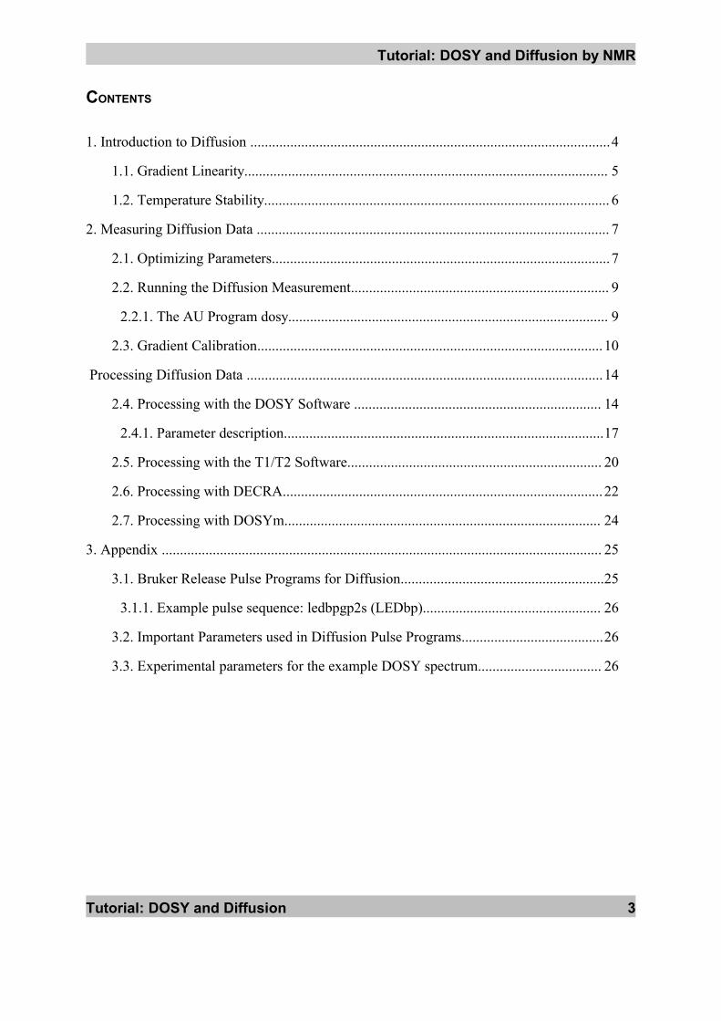
CONTENTS

1. Introduction to Diffusion ...................................................................................................4

1.1. Gradient Linearity.................................................................................................... 5

1.2. Temperature Stability............................................................................................... 6

2. Measuring Diffusion Data ................................................................................................. 7

2.1. Optimizing Parameters.............................................................................................7

2.2. Running the Diffusion Measurement....................................................................... 9

2.2.1. The AU Program dosy........................................................................................ 9

2.3. Gradient Calibration...............................................................................................10

Processing Diffusion Data ..................................................................................................14

2.4. Processing with the DOSY Software .................................................................... 14

2.4.1. Parameter description........................................................................................17

2.5. Processing with the T1/T2 Software...................................................................... 20

2.6. Processing with DECRA........................................................................................22

2.7. Processing with DOSYm....................................................................................... 24

3. Appendix ......................................................................................................................... 25

3.1. Bruker Release Pulse Programs for Diffusion........................................................25

3.1.1. Example pulse sequence: ledbpgp2s (LEDbp)................................................. 26

3.2. Important Parameters used in Diffusion Pulse Programs.......................................26

3.3. Experimental parameters for the example DOSY spectrum.................................. 26

Tutorial: DOSY and Diffusion 3

Introduction to Diffusion

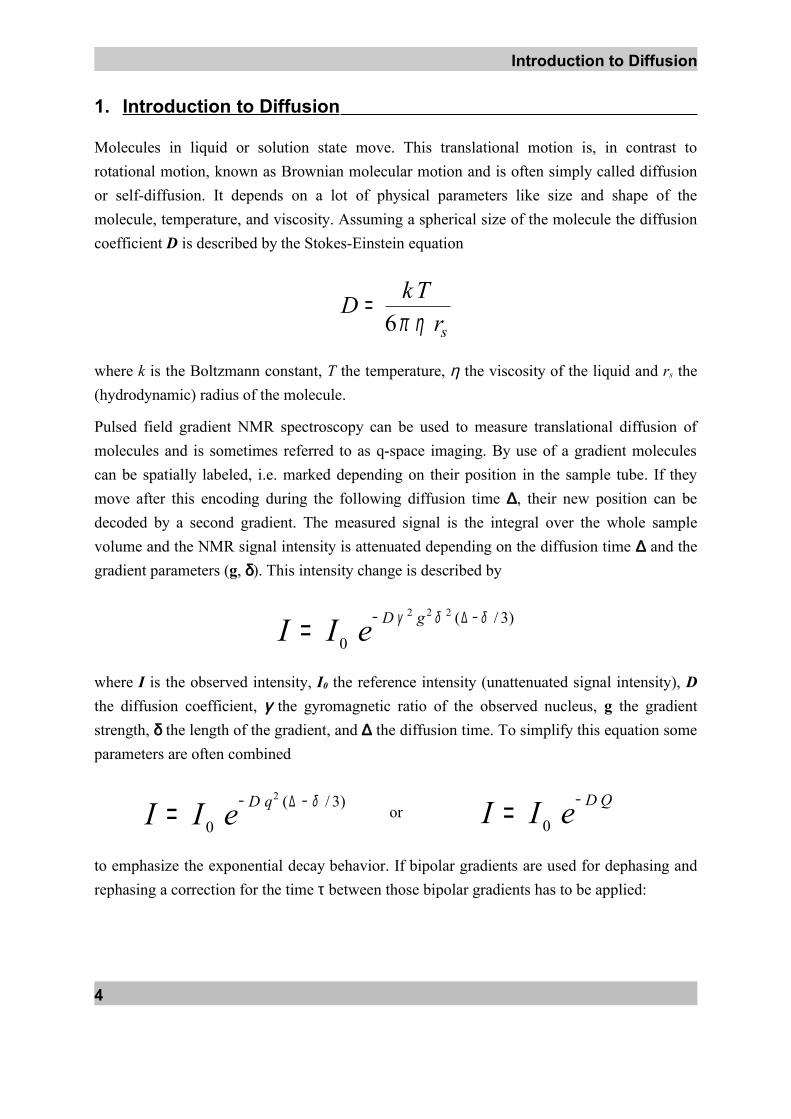
1. Introduction to Diffusion

Molecules in liquid or solution state move. This translational motion is, in contrast to rotational motion, known as Brownian molecular motion and is often simply called diffusion or self-diffusion. It depends on a lot of physical parameters like size and shape of the molecule, temperature, and viscosity. Assuming a spherical size of the molecule the diffusion coefficient D is described by the Stokes-Einstein equation

srTkDηπ6

=

where k is the Boltzmann constant, T the temperature, η the viscosity of the liquid and rs the (hydrodynamic) radius of the molecule.

Pulsed field gradient NMR spectroscopy can be used to measure translational diffusion of molecules and is sometimes referred to as q-space imaging. By use of a gradient molecules can be spatially labeled, i.e. marked depending on their position in the sample tube. If they move after this encoding during the following diffusion time ∆, their new position can be decoded by a second gradient. The measured signal is the integral over the whole sample volume and the NMR signal intensity is attenuated depending on the diffusion time ∆ and the gradient parameters (g, δ). This intensity change is described by

eII gD0

)3/(222

= −∆− δδγ

where I is the observed intensity, I0 the reference intensity (unattenuated signal intensity), D the diffusion coefficient, γ the gyromagnetic ratio of the observed nucleus, g the gradient strength, δ the length of the gradient, and ∆ the diffusion time. To simplify this equation some parameters are often combined

eII qD0

)3/(2

= −∆− δor eII QD

0= −

to emphasize the exponential decay behavior. If bipolar gradients are used for dephasing and rephasing a correction for the time τ between those bipolar gradients has to be applied:

4

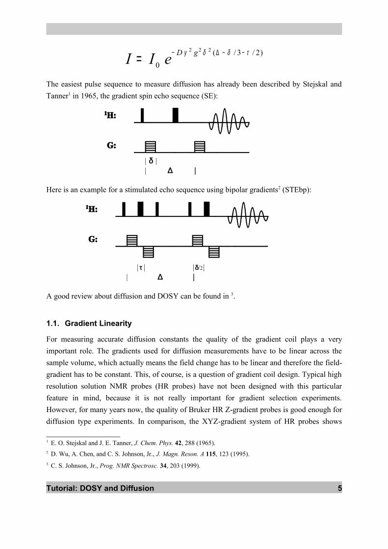
eII gD0

)2/3/(222

= −−∆− τδδγ

The easiest pulse sequence to measure diffusion has already been described by Stejskal and Tanner1 in 1965, the gradient spin echo sequence (SE):

¾ $U'UVWWOÈ V›UU›WWUU

| δ || ∆ |

Here is an example for a stimulated echo sequence using bipolar gradients2 (STEbp):

¾ $'$U$'UWOÈ V›¡UU›¡VWUU

| τ | |δ/2|| ∆ |

A good review about diffusion and DOSY can be found in 3.

1.1. Gradient Linearity

For measuring accurate diffusion constants the quality of the gradient coil plays a very important role. The gradients used for diffusion measurements have to be linear across the sample volume, which actually means the field change has to be linear and therefore the field-gradient has to be constant. This, of course, is a question of gradient coil design. Typical high resolution solution NMR probes (HR probes) have not been designed with this particular feature in mind, because it is not really important for gradient selection experiments. However, for many years now, the quality of Bruker HR Z-gradient probes is good enough for diffusion type experiments. In comparison, the XYZ-gradient system of HR probes shows

1 E. O. Stejskal and J. E. Tanner, J. Chem. Phys. 42, 288 (1965).2 D. Wu, A. Chen, and C. S. Johnson, Jr., J. Magn. Reson. A 115, 123 (1995).3 C. S. Johnson, Jr., Prog. NMR Spectrosc. 34, 203 (1999).


Introduction to Diffusion

some restrictions. The necessary linear range is smaller than the RF-coil height. This limitation can easily be overcome by using a restricted volume, for example with a Shigemi®

tube. A volume of about 1 cm height placed in the center of the RF-coil leads to a NMR signal coming from the most linear area of this gradient system. The difference in quality between a Z-gradient and an XYZ-gradient probe can easily be understood by the limited space in the probe available for the gradient coil(s). This available space can either be used for a single gradient coil or compromises have to be accepted to fit 3 gradient coils into the same space.

1.2. Temperature Stability

One very important experimental parameter when you run a diffusion measurement is a good temperature stability. Having a bad temperature stability easily leads to a temperature gradient along the sample tube, i.e. you have different temperatures at the bottom and the top of the tube. Depending on the viscosity of the solvent and the actual temperature this may introduce convection in your tube: you generated a flow of the solvent. This has the same effect as diffusion, the molecules are moving, but most often much faster than they would do due to diffusion.

If you use low viscosity solvents (like CDCl3) a similar effect occurs if the temperature is too close to the boiling point of the solvent. The solvent strongly evaporates, will condense at the top of the sample tube and either solvent drops will fall down or run down along the tube walls back into the solution. This reflux introduces a flow, which is very similar to convection and will disturb the diffusion measurement.

6

2. Measuring Diffusion Data

To run a diffusion measurement it is necessary to optimize the parameters that determine the decay function described in the previous chapter. To keep the timing constant throughout the whole experiment, we have chosen the gradient strength (g) to be the variable parameter, the diffusion time big delta ∆ and the diffusion gradient length little delta δ are kept constant. All Bruker supplied pulse programs and AU programs are based on this choice. Nevertheless, the processing tools support the evaluation of data acquired by varying either one of the three possible parameters.

2.1. Optimizing Parameters

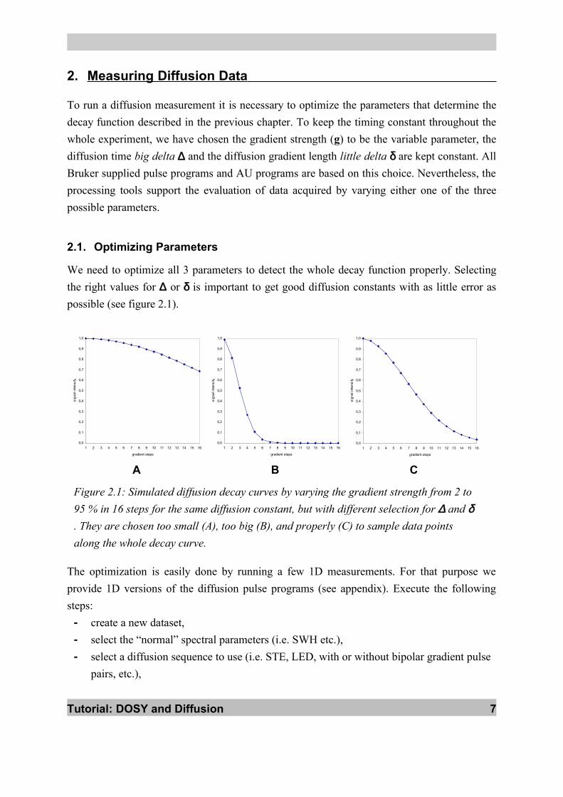
We need to optimize all 3 parameters to detect the whole decay function properly. Selecting the right values for ∆ or δ is important to get good diffusion constants with as little error as possible (see figure 2.1).

0,0

0,1

0,2

0,3

0,4

0,5

0,6

0,7

0,8

0,9

1,0

1 2 3 4 5 6 7 8 9 10 11 12 13 14 15 16

gradient steps

sign

al in

tens

ity

0,0

0,1

0,2

0,3

0,4

0,5

0,6

0,7

0,8

0,9

1,0

1 2 3 4 5 6 7 8 9 10 11 12 13 14 15 16

gradient steps

sign

al in

tens

ity

0,0

0,1

0,2

0,3

0,4

0,5

0,6

0,7

0,8

0,9

1,0

1 2 3 4 5 6 7 8 9 10 11 12 13 14 15 16

gradient steps

sign

al in

tens

ity

A B C

Figure 2.1: Simulated diffusion decay curves by varying the gradient strength from 2 to 95 % in 16 steps for the same diffusion constant, but with different selection for ∆ and δ. They are chosen too small (A), too big (B), and properly (C) to sample data points along the whole decay curve.

The optimization is easily done by running a few 1D measurements. For that purpose we provide 1D versions of the diffusion pulse programs (see appendix). Execute the following steps:- create a new dataset,- select the “normal” spectral parameters (i.e. SWH etc.),- select a diffusion sequence to use (i.e. STE, LED, with or without bipolar gradient pulse

pairs, etc.),


Measuring Diffusion Data

- run a 1D spectrum with start values of 50 – 100 ms for ∆ (d20) and 1 ms for δ (p30) with 2 % (gpz6) amplitude. This spectrum will be used as a reference for the optimization process, so you should store this, for example, in procno 2 (wrp 2). It is important to start with a gradient strength bigger than 0, because you may get unwanted echoes when you don’t apply a gradient. We recommend a start value of 1 to 5 %.

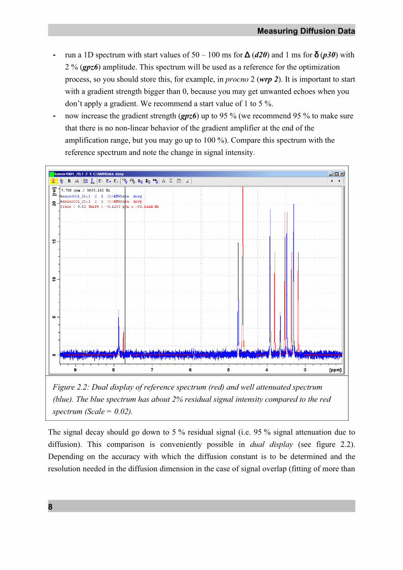
- now increase the gradient strength (gpz6) up to 95 % (we recommend 95 % to make sure that there is no non-linear behavior of the gradient amplifier at the end of the amplification range, but you may go up to 100 %). Compare this spectrum with the reference spectrum and note the change in signal intensity.

Figure 2.2: Dual display of reference spectrum (red) and well attenuated spectrum (blue). The blue spectrum has about 2% residual signal intensity compared to the red spectrum (Scale = 0.02).

The signal decay should go down to 5 % residual signal (i.e. 95 % signal attenuation due to diffusion). This comparison is conveniently possible in dual display (see figure 2.2). Depending on the accuracy with which the diffusion constant is to be determined and the resolution needed in the diffusion dimension in the case of signal overlap (fitting of more than

8

1 component), this value may have to be even smaller. The further you can attenuate the NMR signal, the better is the resolution you can achieve in the resulting DOSY spectrum.

The observable residual signal intensity is, of course, dependent on the signal-to-noise ratio (S/N). For bad S/N you may have to increase the number of scans (NS) or go with less signal attenuation. The smallest signal to be detected (i.e. at highest gradient strength) has to be above the noise. If the signal intensity is already totally gone, reduce the gradient strength (gpz6). If the signal is still to big, you have to increase either the diffusion time ∆ (d20) or the gradient length δ (p30). Increasing δ is favorable, because it results in a bigger effect. δ2 is determining the signal attenuation, while ∆ is only affecting the exponential decay function linearly (see chapter 1). If you change ∆, you have to take the relaxation into account (T1 relaxation for all STE type sequences).

2.2. Running the Diffusion Measurement

After optimizing the parameters you can run the actual diffusion measurement, which is executed as a pseudo-2D acquisition. Instead of incrementing a delay you would do in a “normal” 2D spectrum, the gradient strength is incremented for the indirect dimension. You can easily generate this 2D dataset from the 1D dataset you used for the optimization procedure: - create a new expno with new or edc- switch to a 2D dataset by changing the dimension to 2D (in eda or AcquPars click

on ) - select a 2D pulse program instead of the 1D you used for the optimization

All other parameters are already set correctly, only the gradient ramp has to be generated. For this purpose we provide the AU program dosy.

2.2.1. The AU Program dosy

The AU program dosy is used to calculate the gradient ramp and needs some input parameters that define this ramp. These parameters are the start and the final value of the gradient ramp (0-100), the number of steps (i.e. number of increments = TD1), and the type of ramp (linear l, squared q or exponential e). The program will ask whether the acquisition should be started immediately or not. For automation purposes it is possible to call the AU program non-interactively by passing all parameters on the command line and giving a “y” to start the acquisition. In this case an additional 6th parameter is available, which enables to execute rga before the acquisition is started.



example: xau dosy 2 95 16 l y ystart value 2%, final value 95%, 16 steps, linear ramp, start acquisition, execute rga first.

dosy calculates the gradient ramp file Difframp and stores it in TOPSPINHOME/exp/stan/nmr/lists/gp†. This file is used by the acquisition and contains the gradient strength values in percent gradient amplitude; 100% means maximum current, typically 10 A for the standard high resolution gradient amplifiers (GAB, GREAT 1/10, GREAT 3/10, ACUSTAR, BGPA). To have all the values used by dosy available as status parameters, the start and final value are stored as constants 20 and 21 (CNST20/21) and the ramp is converted into real gradient strength (in G/cm, see below) and stored in the expno of the dataset under the name difflist. This file is necessary for the processing later.

Diffusion experiments don’t have an imaginary part in the diffusion dimension, therefore the acquisition is setup like an QF experiment (FnMODE = QF). dosy requires this parameter to be set and the Bruker pulse programs are written this way. dosy uses the parameter FnMODE in the case of a 3D experiment to try to detect the diffusion dimension. In general, 3D diffusion measurements (i.e. 2 spectroscopic and 1 diffusion dimension) are setup just like any other 3D acquisition. It is strongly recommended to determine the diffusion parameters using a 2D measurement. This is basically the same as running a 2D plane out of the 3D first.

The way to setup, optimize and run a diffusion measurement, as described above, is always the same and is independent from the way the data is processed afterwards using the different methods DOSY, fitting, DECRA or DOSYm. The only important difference: for DECRA it is necessary to select the square ramp type, otherwise you can’t use DECRA as processing method.

2.3. Gradient Calibration

As mentioned above, the AU program dosy calculates the gradient ramp to be used during the diffusion measurement. For the acquisition we specify the gradient strength in percent of the maximum current provided by the gradient amplifier. For high resolution instruments this is typically 10 A, i.e. 100% means 10 A current through the gradient coil. In addition to this typical high resolution instrumentation, stronger amplifiers delivering higher currents and different probes with specialized gradient coils (“diffusion probe”, etc.) are also available.

† TOPSPINHOME (or XWINNMRHOME) is the directory where TopSpin is installed (typically

C:\Bruker\TOPSPIN under Windows and /opt/topspin under Linux).

10

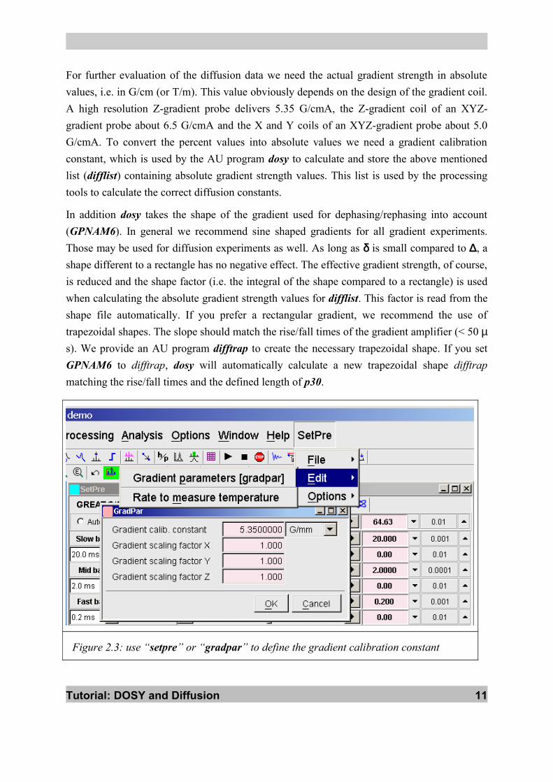
For further evaluation of the diffusion data we need the actual gradient strength in absolute values, i.e. in G/cm (or T/m). This value obviously depends on the design of the gradient coil. A high resolution Z-gradient probe delivers 5.35 G/cmA, the Z-gradient coil of an XYZ-gradient probe about 6.5 G/cmA and the X and Y coils of an XYZ-gradient probe about 5.0 G/cmA. To convert the percent values into absolute values we need a gradient calibration constant, which is used by the AU program dosy to calculate and store the above mentioned list (difflist) containing absolute gradient strength values. This list is used by the processing tools to calculate the correct diffusion constants.

In addition dosy takes the shape of the gradient used for dephasing/rephasing into account (GPNAM6). In general we recommend sine shaped gradients for all gradient experiments. Those may be used for diffusion experiments as well. As long as δ is small compared to ∆, a shape different to a rectangle has no negative effect. The effective gradient strength, of course, is reduced and the shape factor (i.e. the integral of the shape compared to a rectangle) is used when calculating the absolute gradient strength values for difflist. This factor is read from the shape file automatically. If you prefer a rectangular gradient, we recommend the use of trapezoidal shapes. The slope should match the rise/fall times of the gradient amplifier (< 50 µs). We provide an AU program difftrap to create the necessary trapezoidal shape. If you set GPNAM6 to difftrap, dosy will automatically calculate a new trapezoidal shape difftrap matching the rise/fall times and the defined length of p30.

Figure 2.3: use “setpre” or “gradpar” to define the gradient calibration constant



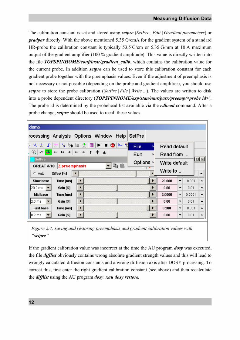
The calibration constant is set and stored using setpre (SetPre | Edit | Gradient parameters) or gradpar directly. With the above mentioned 5.35 G/cmA for the gradient system of a standard HR-probe the calibration constant is typically 53.5 G/cm or 5.35 G/mm at 10 A maximum output of the gradient amplifier (100 % gradient amplitude). This value is directly written into the file TOPSPINHOME/conf/instr/gradient_calib, which contains the calibration value for the current probe. In addition setpre can be used to store this calibration constant for each gradient probe together with the preemphasis values. Even if the adjustment of preemphasis is not necessary or not possible (depending on the probe and gradient amplifier), you should use setpre to store the probe calibration (SetPre | File | Write ...). The values are written to disk into a probe dependent directory (TOPSPINHOME/exp/stan/nmr/parx/preemp/<probe id>). The probe id is determined by the probehead list available via the edhead command. After a probe change, setpre should be used to recall these values.

Figure 2.4: saving and restoring preemphasis and gradient calibration values with “setpre”

If the gradient calibration value was incorrect at the time the AU program dosy was executed, the file difflist obviously contains wrong absolute gradient strength values and this will lead to wrongly calculated diffusion constants and a wrong diffusion axis after DOSY processing. To correct this, first enter the right gradient calibration constant (see above) and then recalculate the difflist using the AU program dosy: xau dosy restore.

12

Processing Diffusion Data

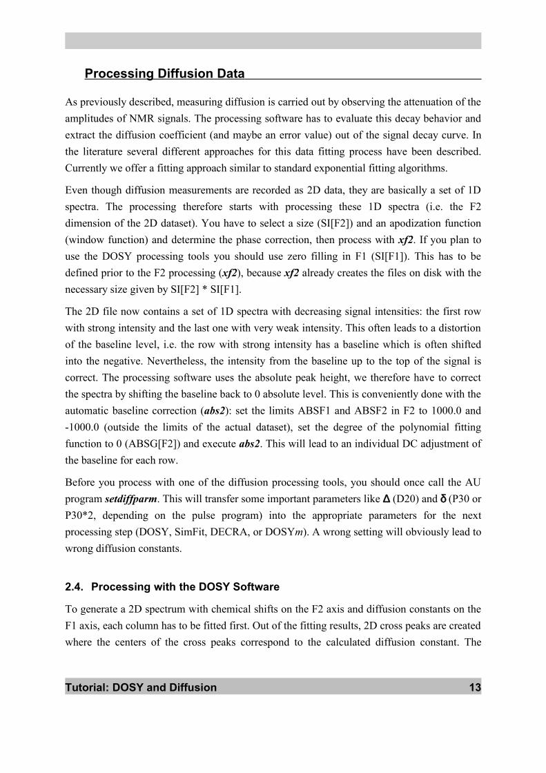
As previously described, measuring diffusion is carried out by observing the attenuation of the amplitudes of NMR signals. The processing software has to evaluate this decay behavior and extract the diffusion coefficient (and maybe an error value) out of the signal decay curve. In the literature several different approaches for this data fitting process have been described. Currently we offer a fitting approach similar to standard exponential fitting algorithms.

Even though diffusion measurements are recorded as 2D data, they are basically a set of 1D spectra. The processing therefore starts with processing these 1D spectra (i.e. the F2 dimension of the 2D dataset). You have to select a size (SI[F2]) and an apodization function (window function) and determine the phase correction, then process with xf2. If you plan to use the DOSY processing tools you should use zero filling in F1 (SI[F1]). This has to be defined prior to the F2 processing (xf2), because xf2 already creates the files on disk with the necessary size given by SI[F2] * SI[F1].

The 2D file now contains a set of 1D spectra with decreasing signal intensities: the first row with strong intensity and the last one with very weak intensity. This often leads to a distortion of the baseline level, i.e. the row with strong intensity has a baseline which is often shifted into the negative. Nevertheless, the intensity from the baseline up to the top of the signal is correct. The processing software uses the absolute peak height, we therefore have to correct the spectra by shifting the baseline back to 0 absolute level. This is conveniently done with the automatic baseline correction (abs2): set the limits ABSF1 and ABSF2 in F2 to 1000.0 and -1000.0 (outside the limits of the actual dataset), set the degree of the polynomial fitting function to 0 (ABSG[F2]) and execute abs2. This will lead to an individual DC adjustment of the baseline for each row.

Before you process with one of the diffusion processing tools, you should once call the AU program setdiffparm. This will transfer some important parameters like ∆ (D20) and δ (P30 or P30*2, depending on the pulse program) into the appropriate parameters for the next processing step (DOSY, SimFit, DECRA, or DOSYm). A wrong setting will obviously lead to wrong diffusion constants.

2.4. Processing with the DOSY Software

To generate a 2D spectrum with chemical shifts on the F2 axis and diffusion constants on the F1 axis, each column has to be fitted first. Out of the fitting results, 2D cross peaks are created where the centers of the cross peaks correspond to the calculated diffusion constant. The



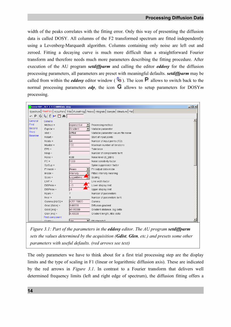
width of the peaks correlates with the fitting error. Only this way of presenting the diffusion data is called DOSY. All columns of the F2 transformed spectrum are fitted independently using a Levenberg-Marquardt algorithm. Columns containing only noise are left out and zeroed. Fitting a decaying curve is much more difficult than a straightforward Fourier transform and therefore needs much more parameters describing the fitting procedure. After execution of the AU program setdiffparm and calling the editor eddosy for the diffusion processing parameters, all parameters are preset with meaningful defaults. setdiffparm may be called from within the eddosy editor window ( ). The icon allows to switch back to the normal processing parameters edp, the icon allows to setup parameters for DOSYm processing.

Figure 3.1: Part of the parameters in the eddosy editor. The AU program setdiffparm sets the values determined by the acquisition (Gdist, Glen, etc.) and presets some other parameters with useful defaults. (red arrows see text)

The only parameters we have to think about for a first trial processing step are the display limits and the type of scaling in F1 (linear or logarithmic diffusion axis). These are indicated by the red arrows in Figure 3.1. In contrast to a Fourier transform that delivers well determined frequency limits (left and right edge of spectrum), the diffusion fitting offers a

14

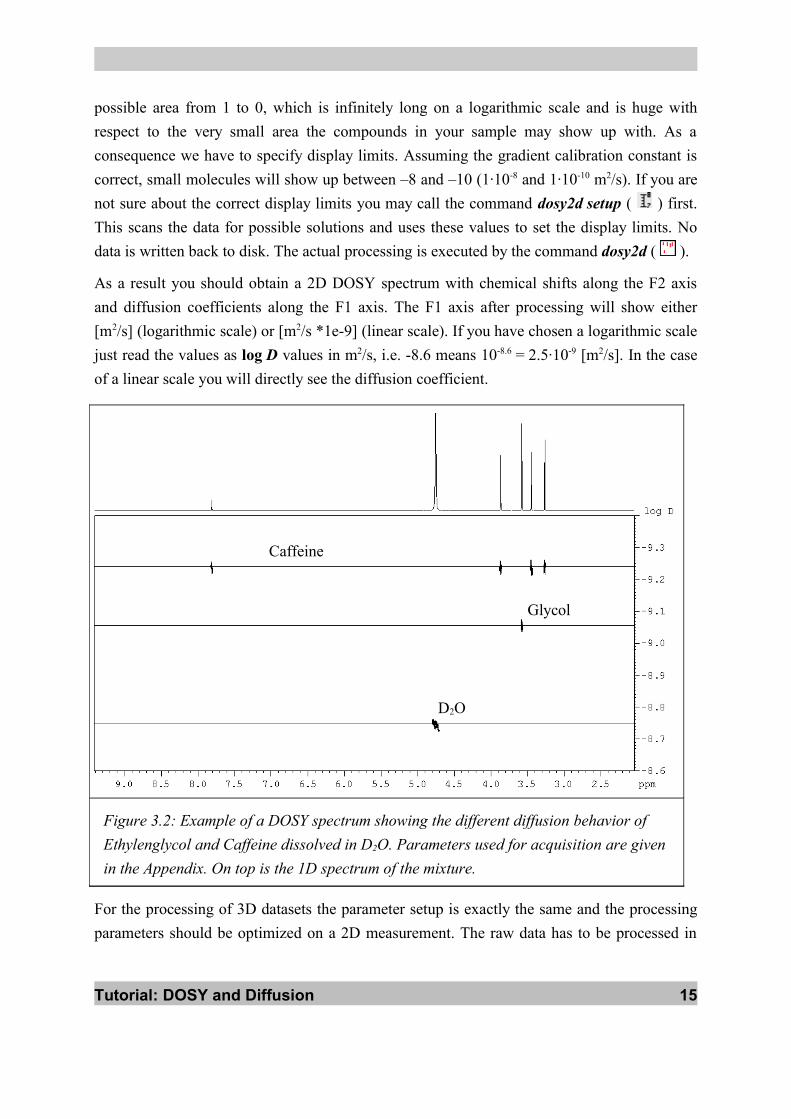
possible area from 1 to 0, which is infinitely long on a logarithmic scale and is huge with respect to the very small area the compounds in your sample may show up with. As a consequence we have to specify display limits. Assuming the gradient calibration constant is correct, small molecules will show up between –8 and –10 (1·10-8 and 1·10-10 m2/s). If you are not sure about the correct display limits you may call the command dosy2d setup ( ) first. This scans the data for possible solutions and uses these values to set the display limits. No data is written back to disk. The actual processing is executed by the command dosy2d ( ).

As a result you should obtain a 2D DOSY spectrum with chemical shifts along the F2 axis and diffusion coefficients along the F1 axis. The F1 axis after processing will show either [m2/s] (logarithmic scale) or [m2/s *1e-9] (linear scale). If you have chosen a logarithmic scale just read the values as log D values in m2/s, i.e. -8.6 means 10-8.6 = 2.5·10-9 [m2/s]. In the case of a linear scale you will directly see the diffusion coefficient.

Figure 3.2: Example of a DOSY spectrum showing the different diffusion behavior of Ethylenglycol and Caffeine dissolved in D2O. Parameters used for acquisition are given in the Appendix. On top is the 1D spectrum of the mixture.

For the processing of 3D datasets the parameter setup is exactly the same and the processing parameters should be optimized on a 2D measurement. The raw data has to be processed in


Caffeine

Glycol

D2O


both spectroscopic dimensions first, i.e. tf3 and tf2 or tf3 and tf1, depending on which direction is the diffusion dimension. The processing for a pseudo-3D DOSY is executed with dosy3d.

2.4.1. Parameter description

ExpVar - variable parameter: This parameter defines the experimental variable. It can take values of "Gradient", "Grad_distance", or "Grad_length", corresponding to the variable gradient strength g (= gradient amplitude), diffusion time big delta ∆ (= gradient distance) and diffusion gradient length little delta δ. It is used to select the proper fitting formula.

Xlist - variable parameter values file name: The values of the experimental variable ExpVar are kept in the specified file <disk>/data/<user>/nmr/<name>/<expno>/<Xlist>. The default value for Xlist is "difflist".

Nstart - start of input points: In some cases, a few data points at the beginning of the curve to be fitted may have wrong values. Nstart allows to exclude them to produce better results.

Ndata - number of input points: Number of points actually used for the fitting. Ndata must be bigger than the number of the fittable parameters Nvar. Nstart+Ndata must not be bigger than TDeff.

Maxiter - maximum number of iterations: Defines the stop condition for the Levenberg-Marquardt iteration loop. Default value is 100.

EPS – tolerance: Another stop condition for the iteration loop. The loop breaks when the RMS deviation of the fit decreases by a value less then EPS. One may understand EPS as "minimal average improvement of fitted point" to be accepted. As we deal with integer data, EPS = 1 is a good candidate for the default value. EPS and Maxiter work together to limit the total processing time. Typically, it takes 20-50 iterations to achieve acceptable convergence and the loop breaks by the EPS condition. But for slowly converging cases, iteration stops after Maxiter cycles.

Nexp - number of exponents to fit: DOSY fitting is able to discover up to three simultaneous decays in the experimental data. This allows overlapping peaks in the spectrum to be resolved in the DOSY dimension. The

16

Nexp parameter defines how many of In and Dn (see below) are taken into account by the fitting.

Noise - noise level calculated by xf2. This parameter cannot be changed by the user and is displayed for convenience only.

PC - noise sensitivity factor: If all intensity values of a data column are smaller than PC * Noise, the column is qualified as pure noise and zeroed on output. Default value is 4.

SpiSup - spike suppression factor: Occasionally, the fit produces unlikely good convergence for some columns resulting in sharp spikes in the DOSY spectrum. The parameter SpiSup allows to set the minimal allowed peak width to a reasonable value = SpiSup * Noise.

F1mode - F1 output data mode: The default value "Peaks" means that the F1 data will be generated as gaussian shaped peaks with the intensities, positions and linewidths corresponding to the fitted intensities, diffusion values and their standard deviations using the Scale as defined by the user. If F1mode has the value "Decays", then the Stejskal-Tanner decays along F1 will be generated corresponding to the fitted parameters. These results may be further fitted by dosy again. The main feature of this mode is the ability to generate simulated diffusion decays with known properties to test the quality of the data.

Imode - fitted intensity meaning: This switch determines whether the calculated peaks in the 2D spectrum will have correct integrals (Imode = Integral, by default) or correct intensities (i.e. peak heights) corresponding to the fitted intensities In (Imode = Intensities).

Scale - scaling in DOSY direction: Sets the axis to linear or logarithmic scale in the DOSY direction.

LWF - line width factor: Allows to adjust the peak width in the DOSY direction by multiplying the calculated width with LWF. This is similar to a line broadening window function (exponential multiplication). A special case is setting LWF = 0. This produces peaks with one pixel width, i.e. the fitting error will not correspond to the width of a cross peak. The default value is 1.



DISPmin, DISPmax - lower and upper display limits for F1: Reasonable values depend on the chosen scale. Can be preset automatically by dosy2d setup.

Npars - number of parameters: Shows the number of parameters used by the fitting, equal to five (Gamma, Grad, Gdist, Glen, Bline) plus two for each fitted decay (In, Dn).

Nvar - number of parameters to fit: Number of fittable parameters with the "vary" tag set to "Yes".

Gamma - gyromagnetic ratio of current nucleus: 4257.64 Hz/G for protons, is preset by the AU program setdiffparm.

Grad - diffusion gradient. Gdist - gradient distance (big delta ∆).Glen - gradient length (little delta δ).

These three values are experimental variables, one of them, defined by ExpVar, had been varied in the experiment. This value is ignored, instead we use Xlist as the source. The other two values were experimental constants.

I1vary - fit intensity: Yes/No I1 - intensity of component 1.I1min - minimum intensity of component 1. I1max - maximum intensity of component 1.

This block of four parameters defines the properties of the first component intensity. I1vary = Yes means this parameter should be fitted, otherwise it is fixed. I1 defines the start value for the fitting. I1min and I1max define limits for the search.

D1vary - fit diffusion coefficient: Yes/No.D1 - diffusion coefficient. D1min - minimum diffusion coefficient. D1max - maximum diffusion coefficient.

Like I1*, define the properties of the first component diffusion coefficient.

18

I2*,I3*,D2*,D3* parameters have the same meaning as I1* and D1* for the second and the third component, respectively.

Bvary,Bline,Bmin,Bmax deal with baseline fitting in the same way as the In* and Dn* parameters. Generally, we recommend to adjust the baseline with TopSpin tools (such as abs2) before the DOSY fitting and set Bvary = No and Bline = 0. The free baseline fitting during the DOSY processing is much less stable.

Note: The user should not overestimate the ability of DOSY to resolve decays with similar constants, especially in presence of noise. Simulations show that the algorithm fails to resolve exponents of the form exp(-x)+2 * exp(-2x) when there is more than 5% noise in the data.

The parameters ExpVar, Xlist, Scale, Gamma, Grad, Gdist, Glen must be set by the user in order to obtain proper results. Other parameters may be automatically preset by the command dosy2d setup. dosy2d setup changes the parameters only, it does not alter the data.

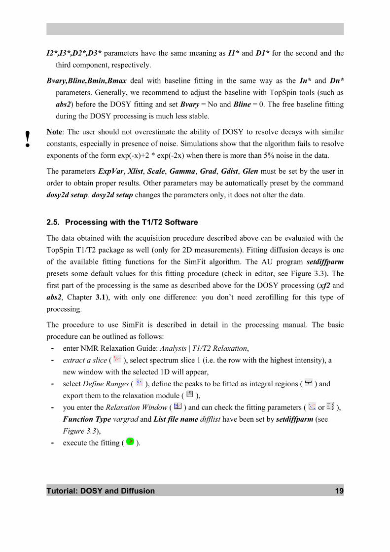
2.5. Processing with the T1/T2 Software

The data obtained with the acquisition procedure described above can be evaluated with the TopSpin T1/T2 package as well (only for 2D measurements). Fitting diffusion decays is one of the available fitting functions for the SimFit algorithm. The AU program setdiffparm presets some default values for this fitting procedure (check in editor, see Figure 3.3). The first part of the processing is the same as described above for the DOSY processing (xf2 and abs2, Chapter 3.1), with only one difference: you don’t need zerofilling for this type of processing.

The procedure to use SimFit is described in detail in the processing manual. The basic procedure can be outlined as follows:- enter NMR Relaxation Guide: Analysis | T1/T2 Relaxation,- extract a slice ( ), select spectrum slice 1 (i.e. the row with the highest intensity), a

new window with the selected 1D will appear,- select Define Ranges ( ), define the peaks to be fitted as integral regions ( ) and

export them to the relaxation module ( ),- you enter the Relaxation Window ( ) and can check the fitting parameters ( or ),

Function Type vargrad and List file name difflist have been set by setdiffparm (see Figure 3.3),

- execute the fitting ( ).


!


Figure 3.3: Part of the parameters in the relaxation parameters editor. The AU program setdiffparm sets the values determined by the acquisition (LITDEL, BIGDEL, etc.) and presets some other parameters with useful defaults.

20

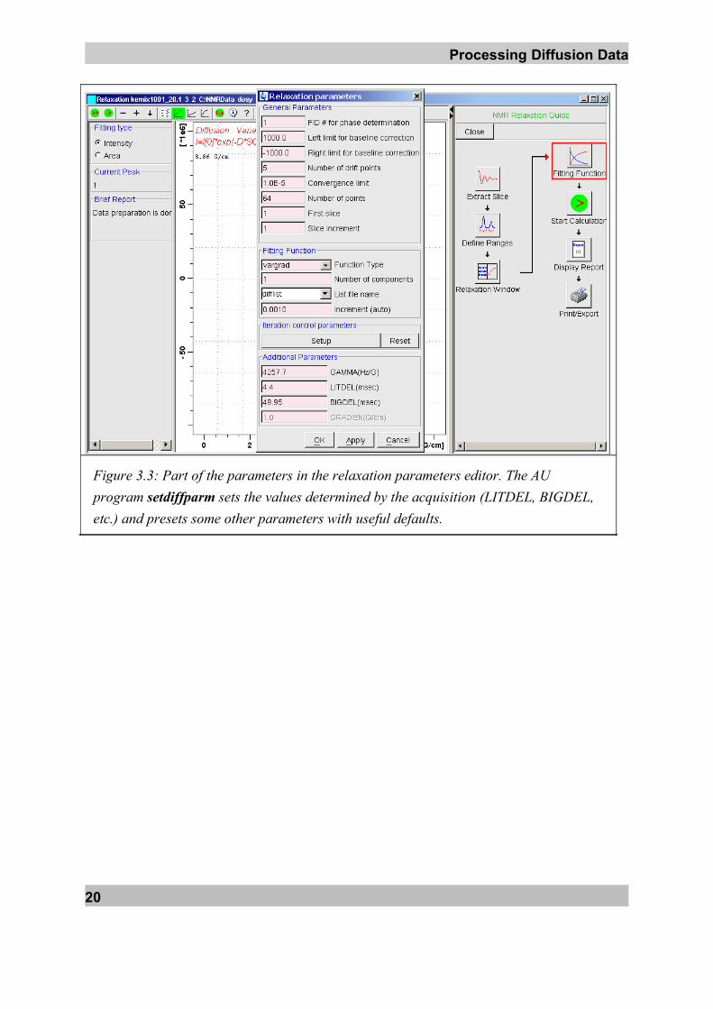
Figure 3.4: TopSpin display after fitting with SimFit (T1/T2 Analysis). The fitting curve for the peak at 3.87 ppm (Caffeine) is shown.

Figure 3.4 shows a typical result after processing with SimFit. The calculated diffusion constant (5.8e-10 m2/s) is the same a shown in the DOSY spectrum (see Figure 3.2):-9.24 [(log)m2/s] ⇒ 10-9.24 = 5.75·10-10 [m2/s].

2.6. Processing with DECRA

DECRA or Direct Exponential Curve Resolution Algorithm is implemented as an AU program named decra. DECRA is based on algorithms described in the original papers by B. Antalek and W. Windig#.

The algorithm provides another means to the analysis of diffusion spectra: instead of nonlinear fitting each 2D column separately, DECRA processes the 2D spectrum as a whole. The result are the 1D subspectra corresponding to the components of the mixture separated

W. Windig, B. Antalek, Chemometrics and Intelligent Laboratory Systems, 37, 241-254 (1997),

B. Antalek, Concepts in Magnetic Resonance, 14 (4), 225-258 (2002).



from each other (almost as LC-NMR, but without LC). In addition to the spectra of the separated components the diffusion constants and the relative amounts of the components are calculated. The present implementation of DECRA as an AU program and the part of the algorithm concerning autodetection of the number of components has been developed by Georgy Salnikov+. Many Thanks to him for this nice work.

The program is easy to use. It requires less parameters than dosy2d, no special setup or prior knowledge is necessary (unlike “dosy2d setup”), and therefore less user experience. Although the resulting 1D spectra might be not as visual as a DOSY spectrum, DECRA produces rather fool-proof results. The short usage instructions one can find, as usual, in the comments at the beginning of the AU program source. Typically you just call decra. You will be asked in which procno the first component spectrum should be saved (it will use the following numbers to save further component spectra). The second question is how many components you expect, the default answer is auto.

From the theory DECRA outperforms dosy2d in the following aspects:- It evaluates the 2D data as a whole thus reducing the probability of artifacts due to bad

data in some particular columns. Particularly, overestimating the number of components in DECRA should be impossible, and the reliability of the results for overlapped peaks is much higher compared to the multiexponential dosy2d fitting. The DECRA algorithm is also more stable than fitting in the presence of big noise.

- In principle, it can achieve better separation of components than DOSY, in particular if the components have similar diffusion coefficients and/or massive regions of overlapped peaks.

- The 1D spectra of separated components produced by DECRA can be integrated and/or phase corrected (if imaginary data were available) after the DECRA processing. The intensities of the distinct subspectra are even comparable with each other so that the concentrations of the components may be estimated.

- The quality of high resolution multiplets in the subspectra separated by DECRA is much better compared to dosy2d, as the DECRA multiplets have undistorted relative intensities.

- In the present implementation, DECRA can in most cases automatically detect the actual number of resolvable components and generate all the corresponding subspectra.

- DECRA is fast: a typical 2D spectrum (32 rows, 16K words each) is processed by DECRA in several seconds. This is independent from the number of components to

+ NMR Group, Novosibirsk Institute of Organic Chemistry SB Russian Academy of Science, Lavrentjeva 9,

630090 Novosibirsk, Russia; [email protected]

22

separate, a monoexponential fitting by dosy2d may take about 10 seconds, a multiexponential fitting even much longer.

- DECRA requires no preset of diffusion limits and therefore no setup phase.

However, DECRA has also a few disadvantages in comparison with dosy2d:- The main drawback is the requirement that data must be acquired using a squared

gradient ramp. Therefore, if the diffusion coefficients of the components differ a lot, several measurements may be necessary to get the best separation of subspectra of all components.

- As DECRA has to load the whole data matrix into memory, it is restricted to 2D processing only (very big spectra can overload the computer resources). Memory requirements are therefore much bigger than for DOSY.

- The sensitivity to systematic errors (incomplete relaxation, inaccurate gradients, etc.) resulting in the unability to resolve some of the components may be higher. But how sensitive it really is in comparison with dosy2d, is not yet tested.

In practice, as quite often observed, the reality does not show what the theory promised. You will not always get subspectra with clear separation of different components of a mixture.

2.7. Processing with DOSYm

DOSYm (Diffusion Ordered SpectroscopY module) is an efficient, easy to use, processing module especially designed for Bruker TopSpin NMR Software. Similar to the above described DOSY processing (chapter 3.1.), it delivers DOSY spectra. Instead of a plain fitting method, it uses a maximum entropy algorithm to obtain the result. For a complex mixture of small molecules with highly overlapping signals, maximum entropy processing typically is able to distinguish much better between the different compounds. Further information is available in the DOSYm manual. TopSpin provides the interface to use this module, but the module is not part of the TopSpin program suite, you have to buy a license separately. Bruker is able to deliver an evaluation version to you.

DOSYm is a trademark of NMRtec S.A.S., France: http://www.nmrtec.com


Appendix

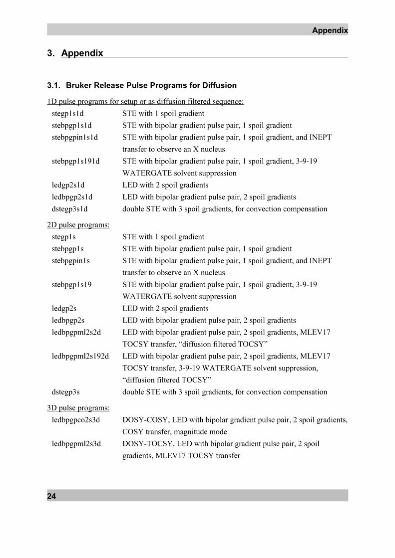
3. Appendix

3.1. Bruker Release Pulse Programs for Diffusion

1D pulse programs for setup or as diffusion filtered sequence:stegp1s1d STE with 1 spoil gradientstebpgp1s1d STE with bipolar gradient pulse pair, 1 spoil gradientstebpgpin1s1d STE with bipolar gradient pulse pair, 1 spoil gradient, and INEPT

transfer to observe an X nucleusstebpgp1s191d STE with bipolar gradient pulse pair, 1 spoil gradient, 3-9-19

WATERGATE solvent suppressionledgp2s1d LED with 2 spoil gradientsledbpgp2s1d LED with bipolar gradient pulse pair, 2 spoil gradientsdstegp3s1d double STE with 3 spoil gradients, for convection compensation

2D pulse programs:stegp1s STE with 1 spoil gradientstebpgp1s STE with bipolar gradient pulse pair, 1 spoil gradientstebpgpin1s STE with bipolar gradient pulse pair, 1 spoil gradient, and INEPT

transfer to observe an X nucleusstebpgp1s19 STE with bipolar gradient pulse pair, 1 spoil gradient, 3-9-19

WATERGATE solvent suppressionledgp2s LED with 2 spoil gradientsledbpgp2s LED with bipolar gradient pulse pair, 2 spoil gradientsledbpgpml2s2d LED with bipolar gradient pulse pair, 2 spoil gradients, MLEV17

TOCSY transfer, “diffusion filtered TOCSY”ledbpgpml2s192d LED with bipolar gradient pulse pair, 2 spoil gradients, MLEV17

TOCSY transfer, 3-9-19 WATERGATE solvent suppression, “diffusion filtered TOCSY”

dstegp3s double STE with 3 spoil gradients, for convection compensation

3D pulse programs:ledbpgpco2s3d DOSY-COSY, LED with bipolar gradient pulse pair, 2 spoil gradients,

COSY transfer, magnitude modeledbpgpml2s3d DOSY-TOCSY, LED with bipolar gradient pulse pair, 2 spoil

gradients, MLEV17 TOCSY transfer

24

ledbpgpno3s3d DOSY-NOESY, LED with bipolar gradient pulse pair, 2 spoil gradients, NOESY transfer

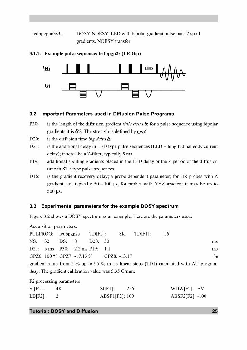
3.1.1. Example pulse sequence: ledbpgp2s (LEDbp)

LED¾ $'$UU$'$V$WOÈ V›¡V³VU›¡W³WVUUW

3.2. Important Parameters used in Diffusion Pulse Programs

P30: is the length of the diffusion gradient little delta δ; for a pulse sequence using bipolar gradients it is δ/2. The strength is defined by gpz6.

D20: is the diffusion time big delta ∆. D21: is the additional delay in LED type pulse sequences (LED = longitudinal eddy current

delay); it acts like a Z-filter; typically 5 ms.P19: additional spoiling gradients placed in the LED delay or the Z period of the diffusion

time in STE type pulse sequences.D16: is the gradient recovery delay; a probe dependent parameter; for HR probes with Z

gradient coil typically 50 – 100 µs, for probes with XYZ gradient it may be up to 500 µs.

3.3. Experimental parameters for the example DOSY spectrum

Figure 3.2 shows a DOSY spectrum as an example. Here are the parameters used.

Acquisition parameters:PULPROG: ledbpgp2s TD[F2]: 8K TD[F1]: 16NS: 32 DS: 8 D20: 50 msD21: 5 ms P30: 2.2 ms P19: 1.1 msGPZ6: 100 % GPZ7: -17.13 % GPZ8: -13.17 %gradient ramp from 2 % up to 95 % in 16 linear steps (TD1) calculated with AU program dosy. The gradient calibration value was 5.35 G/mm.

F2 processing parameters:SI[F2]: 4K SI[F1]: 256 WDW[F2]: EMLB[F2]: 2 ABSF1[F2]: 100 ABSF2[F2]: -100


Appendix

ABSG[F2]: 0execute xf2 followed by abs2.

DOSY processing parameters (only non-default values given):PC: 10 Scale: Logarithmic LWF: 5DISPmin: -10 DISPmax: -8 Gdist: 49.95 msGlen: 4.4 msexecute dosy2d.

26

Documents

DOSY and Diffusion by NMR - Chemistry | University of ... · reproduction of manual contents, without written permission of the publishers, or translation ... Tutorial: DOSY and Diffusion