CETSA

Linear Model Walkthrough

Sigmoidal Model Walkthrough

DOSCHEDA Manual

CETSA

Linear Model Walkthrough

Sigmoidal Model Walkthrough

DOSCHEDA 1.0 Manual andWalkthroughBruno Contrino and Piero Ricchiuto

February 2017

In this document there are three chapters:

1. DOSCHEDA Manual

2. CETSA Manual

3. Linear Model Walkthrough

4. Sigmoidal Model Walkthrough

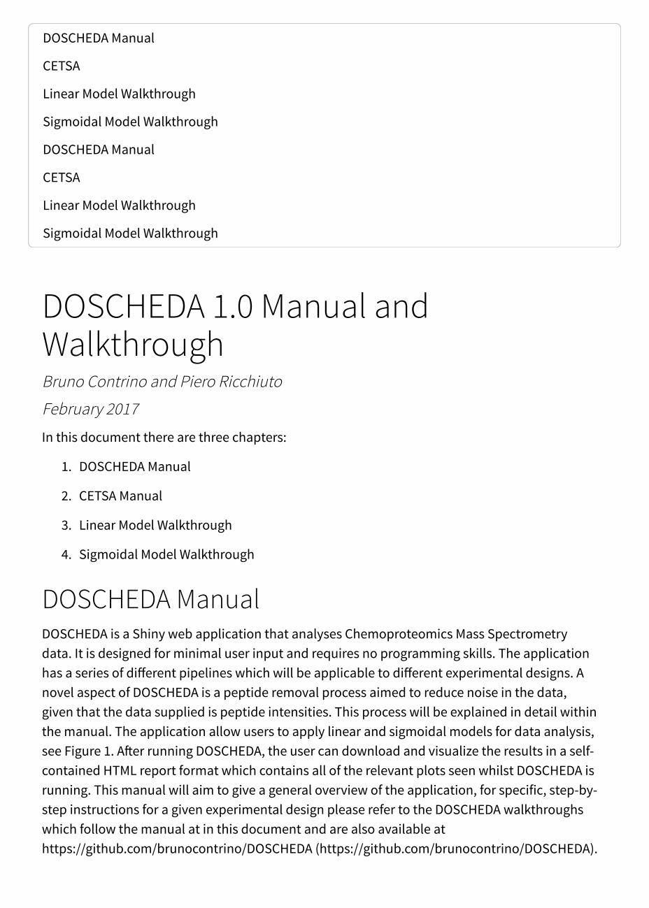
DOSCHEDA ManualDOSCHEDA is a Shiny web application that analyses Chemoproteomics Mass Spectrometrydata. It is designed for minimal user input and requires no programming skills. The applicationhas a series of different pipelines which will be applicable to different experimental designs. Anovel aspect of DOSCHEDA is a peptide removal process aimed to reduce noise in the data,given that the data supplied is peptide intensities. This process will be explained in detail withinthe manual. The application allow users to apply linear and sigmoidal models for data analysis,see Figure 1. After running DOSCHEDA, the user can download and visualize the results in a self-contained HTML report format which contains all of the relevant plots seen whilst DOSCHEDA isrunning. This manual will aim to give a general overview of the application, for specific, step-by-step instructions for a given experimental design please refer to the DOSCHEDA walkthroughswhich follow the manual at in this document and are also available athttps://github.com/brunocontrino/DOSCHEDA (https://github.com/brunocontrino/DOSCHEDA).

DOSCHEDA Manual

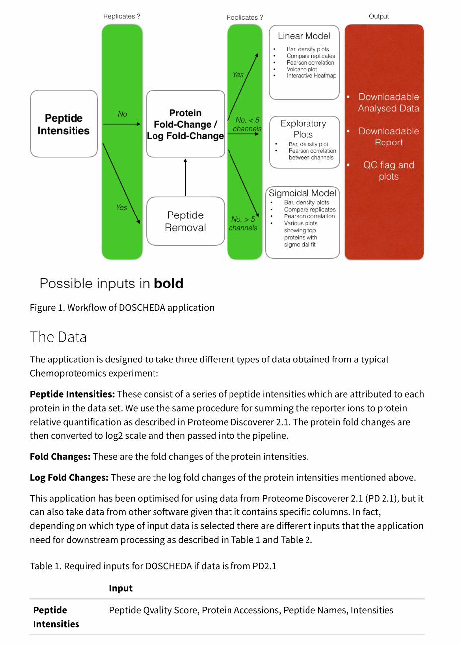
Figure 1. Workflow of DOSCHEDA application

The DataThe application is designed to take three different types of data obtained from a typicalChemoproteomics experiment:

Peptide Intensities: These consist of a series of peptide intensities which are attributed to eachprotein in the data set. We use the same procedure for summing the reporter ions to proteinrelative quantification as described in Proteome Discoverer 2.1. The protein fold changes arethen converted to log2 scale and then passed into the pipeline.

Fold Changes: These are the fold changes of the protein intensities.

Log Fold Changes: These are the log fold changes of the protein intensities mentioned above.

This application has been optimised for using data from Proteome Discoverer 2.1 (PD 2.1), but itcan also take data from other software given that it contains specific columns. In fact,depending on which type of input data is selected there are different inputs that the applicationneed for downstream processing as described in Table 1 and Table 2.

Table 1. Required inputs for DOSCHEDA if data is from PD2.1

Input

PeptideIntensities

Peptide Qvality Score, Protein Accessions, Peptide Names, Intensities

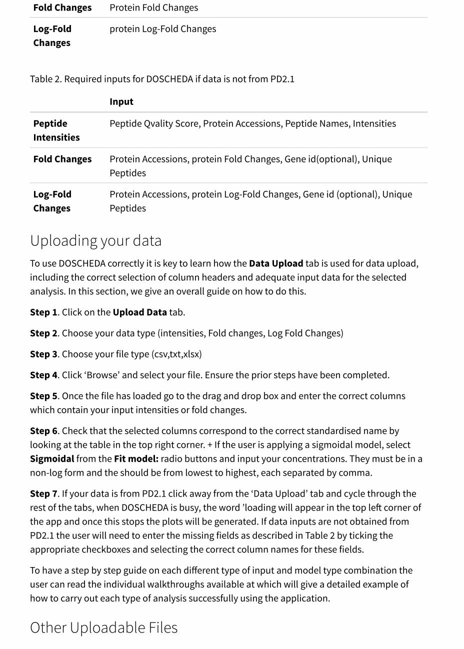
Fold Changes Protein Fold Changes

Log-FoldChanges

protein Log-Fold Changes

Table 2. Required inputs for DOSCHEDA if data is not from PD2.1

Input

PeptideIntensities

Peptide Qvality Score, Protein Accessions, Peptide Names, Intensities

Fold Changes Protein Accessions, protein Fold Changes, Gene id(optional), UniquePeptides

Log-FoldChanges

Protein Accessions, protein Log-Fold Changes, Gene id (optional), UniquePeptides

Uploading your dataTo use DOSCHEDA correctly it is key to learn how the Data Upload tab is used for data upload,including the correct selection of column headers and adequate input data for the selectedanalysis. In this section, we give an overall guide on how to do this.

Step 1. Click on the Upload Data tab.

Step 2. Choose your data type (intensities, Fold changes, Log Fold Changes)

Step 3. Choose your file type (csv,txt,xlsx)

Step 4. Click ‘Browse’ and select your file. Ensure the prior steps have been completed.

Step 5. Once the file has loaded go to the drag and drop box and enter the correct columnswhich contain your input intensities or fold changes.

Step 6. Check that the selected columns correspond to the correct standardised name bylooking at the table in the top right corner. + If the user is applying a sigmoidal model, selectSigmoidal from the Fit model: radio buttons and input your concentrations. They must be in anon-log form and the should be from lowest to highest, each separated by comma.

Step 7. If your data is from PD2.1 click away from the ‘Data Upload’ tab and cycle through therest of the tabs, when DOSCHEDA is busy, the word ’loading will appear in the top left corner ofthe app and once this stops the plots will be generated. If data inputs are not obtained fromPD2.1 the user will need to enter the missing fields as described in Table 2 by ticking theappropriate checkboxes and selecting the correct column names for these fields.

To have a step by step guide on each different type of input and model type combination theuser can read the individual walkthroughs available at which will give a detailed example ofhow to carry out each type of analysis successfully using the application.

Other Uploadable Files

There are two other possible upload files that DOSCHEDA has a functionality for, a proteinaccession to gene symbol ID (two columns file) and a list of custom gene symbol IDs(e.g. Kinases “CDK9”) to compare with the pull-down proteome in your data, the default is a listof kinases that have been taken from the literature.

DOSCHEDA uses Intermine to map Uniprot accession number to gene symbol ID. Should theuser wish to by-pass DOSCHEDA mapping it can be done by uploading a custom 2 columns file(accession to gene symbol ID). Intermine files are updated regularly and should be able toprovide the user with the most up-to-date conversions.

The Include file check box visible in the Venn tab within the Box and Density plots tab willsimply let the user visualise the intersection between the uploaded custom list of proteins andthe pull-down proteome in your data. This is not crucial to the DOSCHEDA pipeline and shouldonly be used if the user has this specific requirement.

Downloading your ResultsFrom the ‘Downloads’ tab users can save their processed data by clicking on the ‘DownloadData’ button. Also in the same tab, the ‘Download Report’ button enables users to download anHTML report containing all the plots seen in the analysis with descriptions as well as otherimportant information such as the options the user has used during the workflow including thenumber of channels (e.g. concentrations), replicates and the statistical fit applied for the dataanalysis.

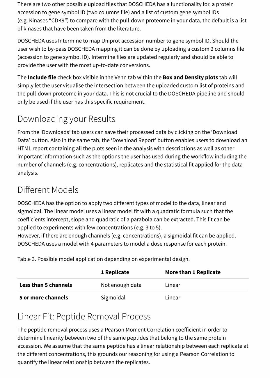
Different ModelsDOSCHEDA has the option to apply two different types of model to the data, linear andsigmoidal. The linear model uses a linear model fit with a quadratic formula such that thecoefficients intercept, slope and quadratic of a parabola can be extracted. This fit can beapplied to experiments with few concentrations (e.g. 3 to 5).However, if there are enough channels (e.g. concentrations), a sigmoidal fit can be applied.DOSCHEDA uses a model with 4 parameters to model a dose response for each protein.

Table 3. Possible model application depending on experimental design.

1 Replicate More than 1 Replicate

Less than 5 channels Not enough data Linear

5 or more channels Sigmoidal Linear

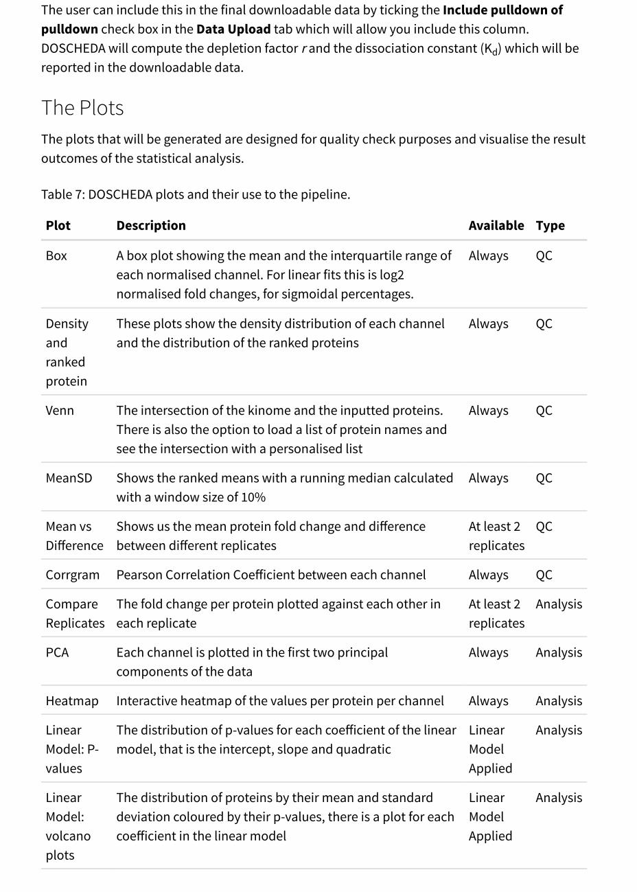
Linear Fit: Peptide Removal ProcessThe peptide removal process uses a Pearson Moment Correlation coefficient in order todetermine linearity between two of the same peptides that belong to the same proteinaccession. We assume that the same peptide has a linear relationship between each replicate atthe different concentrations, this grounds our reasoning for using a Pearson Correlation toquantify the linear relationship between the replicates.

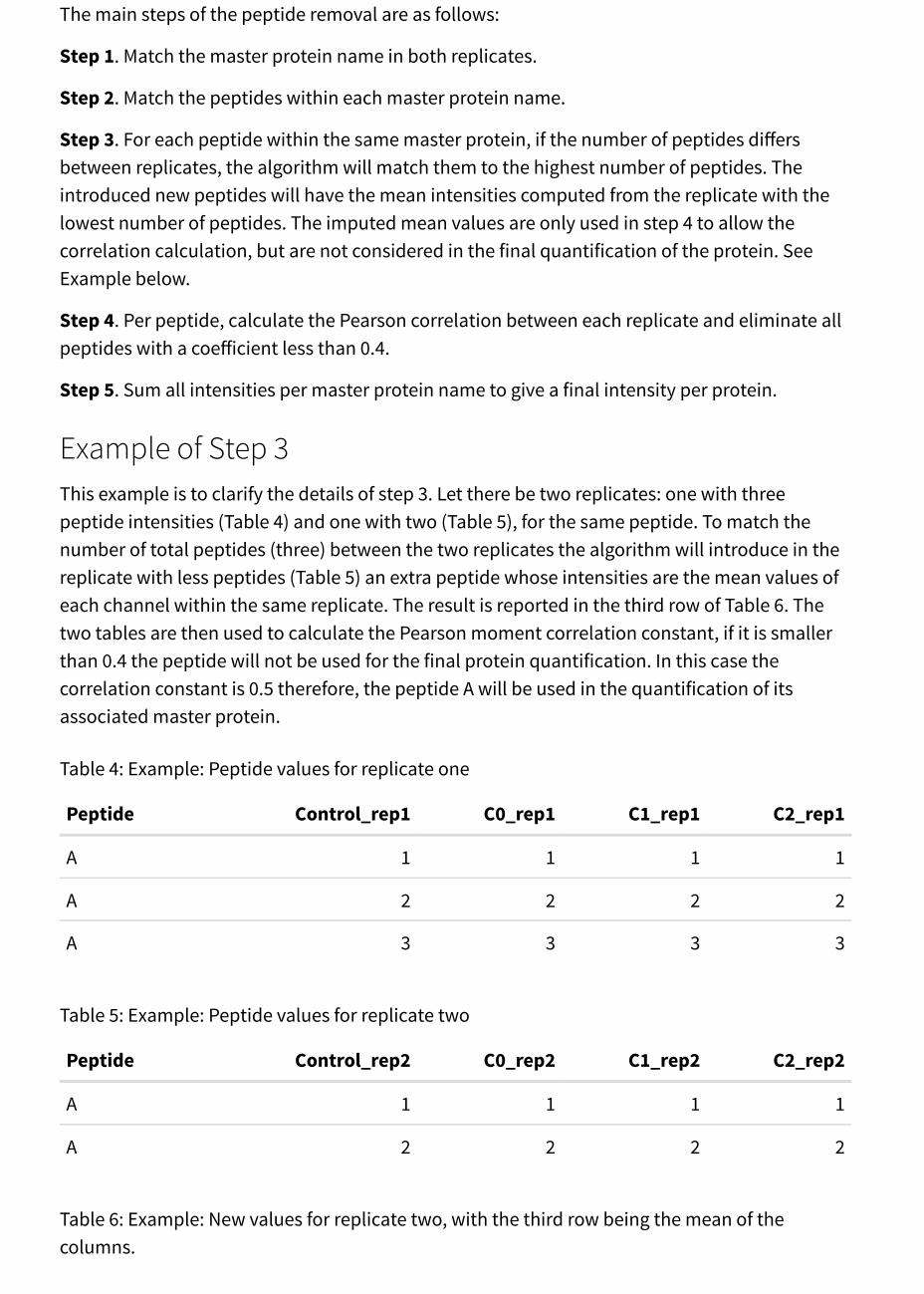
The main steps of the peptide removal are as follows:

Step 1. Match the master protein name in both replicates.

Step 2. Match the peptides within each master protein name.

Step 3. For each peptide within the same master protein, if the number of peptides differsbetween replicates, the algorithm will match them to the highest number of peptides. Theintroduced new peptides will have the mean intensities computed from the replicate with thelowest number of peptides. The imputed mean values are only used in step 4 to allow thecorrelation calculation, but are not considered in the final quantification of the protein. SeeExample below.

Step 4. Per peptide, calculate the Pearson correlation between each replicate and eliminate allpeptides with a coefficient less than 0.4.

Step 5. Sum all intensities per master protein name to give a final intensity per protein.

Example of Step 3This example is to clarify the details of step 3. Let there be two replicates: one with threepeptide intensities (Table 4) and one with two (Table 5), for the same peptide. To match thenumber of total peptides (three) between the two replicates the algorithm will introduce in thereplicate with less peptides (Table 5) an extra peptide whose intensities are the mean values ofeach channel within the same replicate. The result is reported in the third row of Table 6. Thetwo tables are then used to calculate the Pearson moment correlation constant, if it is smallerthan 0.4 the peptide will not be used for the final protein quantification. In this case thecorrelation constant is 0.5 therefore, the peptide A will be used in the quantification of itsassociated master protein.

Table 4: Example: Peptide values for replicate one

Peptide Control_rep1 C0_rep1 C1_rep1 C2_rep1

A 1 1 1 1

A 2 2 2 2

A 3 3 3 3

Table 5: Example: Peptide values for replicate two

Peptide Control_rep2 C0_rep2 C1_rep2 C2_rep2

A 1 1 1 1

A 2 2 2 2

Table 6: Example: New values for replicate two, with the third row being the mean of thecolumns.

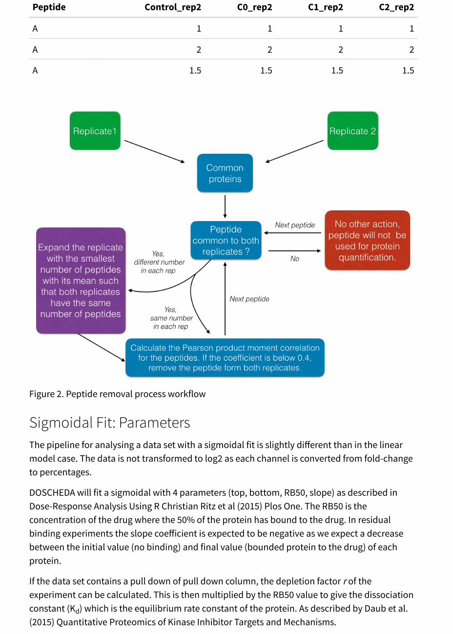
Peptide Control_rep2 C0_rep2 C1_rep2 C2_rep2

A 1 1 1 1

A 2 2 2 2

A 1.5 1.5 1.5 1.5

Figure 2. Peptide removal process workflow

Sigmoidal Fit: ParametersThe pipeline for analysing a data set with a sigmoidal fit is slightly different than in the linearmodel case. The data is not transformed to log2 as each channel is converted from fold-changeto percentages.

DOSCHEDA will fit a sigmoidal with 4 parameters (top, bottom, RB50, slope) as described inDose-Response Analysis Using R Christian Ritz et al (2015) Plos One. The RB50 is theconcentration of the drug where the 50% of the protein has bound to the drug. In residualbinding experiments the slope coefficient is expected to be negative as we expect a decreasebetween the initial value (no binding) and final value (bounded protein to the drug) of eachprotein.

If the data set contains a pull down of pull down column, the depletion factor r of theexperiment can be calculated. This is then multiplied by the RB50 value to give the dissociationconstant (K ) which is the equilibrium rate constant of the protein. As described by Daub et al.(2015) Quantitative Proteomics of Kinase Inhibitor Targets and Mechanisms.

d

The user can include this in the final downloadable data by ticking the Include pulldown ofpulldown check box in the Data Upload tab which will allow you include this column.DOSCHEDA will compute the depletion factor r and the dissociation constant (K ) which will bereported in the downloadable data.

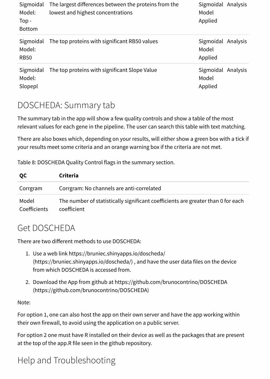
The PlotsThe plots that will be generated are designed for quality check purposes and visualise the resultoutcomes of the statistical analysis.

Table 7: DOSCHEDA plots and their use to the pipeline.

Plot Description Available Type

Box A box plot showing the mean and the interquartile range ofeach normalised channel. For linear fits this is log2normalised fold changes, for sigmoidal percentages.

Always QC

Densityandrankedprotein

These plots show the density distribution of each channeland the distribution of the ranked proteins

Always QC

Venn The intersection of the kinome and the inputted proteins.There is also the option to load a list of protein names andsee the intersection with a personalised list

Always QC

MeanSD Shows the ranked means with a running median calculatedwith a window size of 10%

Always QC

Mean vsDifference

Shows us the mean protein fold change and differencebetween different replicates

At least 2replicates

QC

Corrgram Pearson Correlation Coefficient between each channel Always QC

CompareReplicates

The fold change per protein plotted against each other ineach replicate

At least 2replicates

Analysis

PCA Each channel is plotted in the first two principalcomponents of the data

Always Analysis

Heatmap Interactive heatmap of the values per protein per channel Always Analysis

LinearModel: P-values

The distribution of p-values for each coefficient of the linearmodel, that is the intercept, slope and quadratic

LinearModelApplied

Analysis

LinearModel:volcanoplots

The distribution of proteins by their mean and standarddeviation coloured by their p-values, there is a plot for eachcoefficient in the linear model

LinearModelApplied

Analysis

d

SigmoidalModel:Top -Bottom

The largest differences between the proteins from thelowest and highest concentrations

SigmoidalModelApplied

Analysis

SigmoidalModel:RB50

The top proteins with significant RB50 values SigmoidalModelApplied

Analysis

SigmoidalModel:Slopepl

The top proteins with significant Slope Value SigmoidalModelApplied

Analysis

DOSCHEDA: Summary tabThe summary tab in the app will show a few quality controls and show a table of the mostrelevant values for each gene in the pipeline. The user can search this table with text matching.

There are also boxes which, depending on your results, will either show a green box with a tick ifyour results meet some criteria and an orange warning box if the criteria are not met.

Table 8: DOSCHEDA Quality Control flags in the summary section.

QC Criteria

Corrgram Corrgram: No channels are anti-correlated

ModelCoefficients

The number of statistically significant coefficients are greater than 0 for eachcoefficient

Get DOSCHEDAThere are two different methods to use DOSCHEDA:

1. Use a web link https://bruniec.shinyapps.io/doscheda/(https://bruniec.shinyapps.io/doscheda/) , and have the user data files on the devicefrom which DOSCHEDA is accessed from.

2. Download the App from github at https://github.com/brunocontrino/DOSCHEDA(https://github.com/brunocontrino/DOSCHEDA)

Note:

For option 1, one can also host the app on their own server and have the app working withintheir own firewall, to avoid using the application on a public server.

For option 2 one must have R installed on their device as well as the packages that are presentat the top of the app.R file seen in the github repository.

Help and Troubleshooting

Please feel free to contact us at piero.ricchiuto@astrazeneca.com(mailto:piero.ricchiuto@astrazeneca.com) for feedbacks or unexpected isssues.

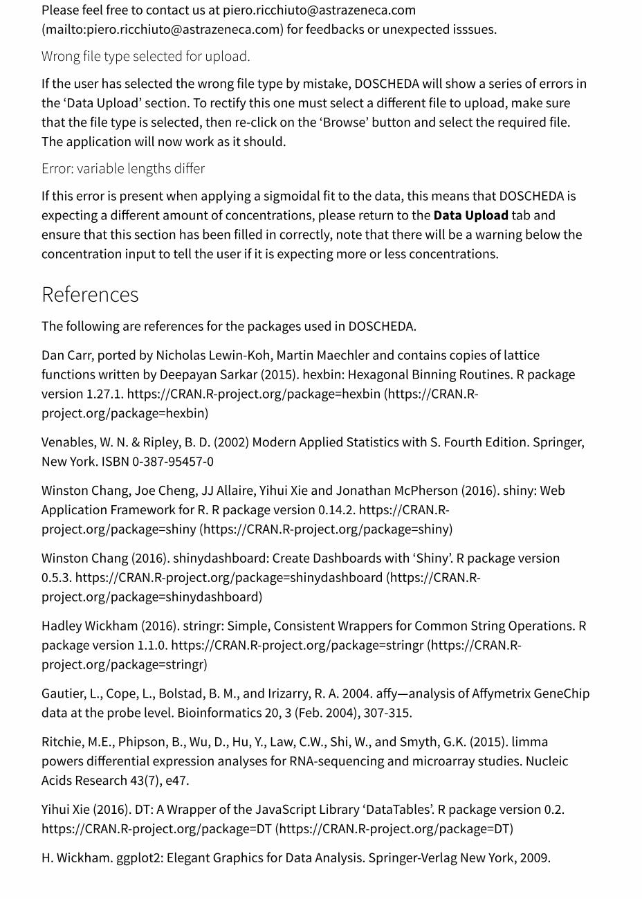
Wrong file type selected for upload.

If the user has selected the wrong file type by mistake, DOSCHEDA will show a series of errors inthe ‘Data Upload’ section. To rectify this one must select a different file to upload, make surethat the file type is selected, then re-click on the ‘Browse’ button and select the required file.The application will now work as it should.

Error: variable lengths differ

If this error is present when applying a sigmoidal fit to the data, this means that DOSCHEDA isexpecting a different amount of concentrations, please return to the Data Upload tab andensure that this section has been filled in correctly, note that there will be a warning below theconcentration input to tell the user if it is expecting more or less concentrations.

ReferencesThe following are references for the packages used in DOSCHEDA.

Dan Carr, ported by Nicholas Lewin-Koh, Martin Maechler and contains copies of latticefunctions written by Deepayan Sarkar (2015). hexbin: Hexagonal Binning Routines. R packageversion 1.27.1. https://CRAN.R-project.org/package=hexbin (https://CRAN.R-project.org/package=hexbin)

Venables, W. N. & Ripley, B. D. (2002) Modern Applied Statistics with S. Fourth Edition. Springer,New York. ISBN 0-387-95457-0

Winston Chang, Joe Cheng, JJ Allaire, Yihui Xie and Jonathan McPherson (2016). shiny: WebApplication Framework for R. R package version 0.14.2. https://CRAN.R-project.org/package=shiny (https://CRAN.R-project.org/package=shiny)

Winston Chang (2016). shinydashboard: Create Dashboards with ‘Shiny’. R package version0.5.3. https://CRAN.R-project.org/package=shinydashboard (https://CRAN.R-project.org/package=shinydashboard)

Hadley Wickham (2016). stringr: Simple, Consistent Wrappers for Common String Operations. Rpackage version 1.1.0. https://CRAN.R-project.org/package=stringr (https://CRAN.R-project.org/package=stringr)

Gautier, L., Cope, L., Bolstad, B. M., and Irizarry, R. A. 2004. affy—analysis of Affymetrix GeneChipdata at the probe level. Bioinformatics 20, 3 (Feb. 2004), 307-315.

Ritchie, M.E., Phipson, B., Wu, D., Hu, Y., Law, C.W., Shi, W., and Smyth, G.K. (2015). limmapowers differential expression analyses for RNA-sequencing and microarray studies. NucleicAcids Research 43(7), e47.

Yihui Xie (2016). DT: A Wrapper of the JavaScript Library ‘DataTables’. R package version 0.2.https://CRAN.R-project.org/package=DT (https://CRAN.R-project.org/package=DT)

H. Wickham. ggplot2: Elegant Graphics for Data Analysis. Springer-Verlag New York, 2009.

Wolfgang Huber, Anja von Heydebreck, Holger Sueltmann, Annemarie Poustka and MartinVingron. Variance Stabilization Applied to Microarray Data Calibration and to the Quantificationof Differential Expression. Bioinformatics 18, S96-S104 (2002).

Baptiste Auguie (2016). gridExtra: Miscellaneous Functions for “Grid” Graphics. R packageversion 2.2.1. https://CRAN.R-project.org/package=gridExtra (https://CRAN.R-project.org/package=gridExtra)

Sarkar, Deepayan (2008) Lattice: Multivariate Data Visualization with R. Springer, New York.ISBN 978-0-387-75968-5

Kevin Wright (2016). corrgram: Plot a Correlogram. R package version 1.9. https://CRAN.R-project.org/package=corrgram (https://CRAN.R-project.org/package=corrgram)

Jan Graffelman (2013). calibrate: Calibration of Scatterplot and Biplot Axes. R package version1.7.2. https://CRAN.R-project.org/package=calibrate (https://CRAN.R-project.org/package=calibrate)

Hadley Wickham (2007). Reshaping Data with the reshape Package. Journal of StatisticalSoftware, 21(12), 1-20. URL http://www.jstatsoft.org/v21/i12/(http://www.jstatsoft.org/v21/i12/).

Hadley Wickham (2016). readxl: Read Excel Files. R package version 0.1.1. https://CRAN.R-project.org/package=readxl (https://CRAN.R-project.org/package=readxl)

Hadley Wickham (2016). lazyeval: Lazy (Non-Standard) Evaluation. R package version 0.2.0.https://CRAN.R-project.org/package=lazyeval (https://CRAN.R-project.org/package=lazyeval)

Ritz, C., Baty, F., Streibig, J. C., Gerhard, D. (2015) Dose-Response Analysis Using R PLOS ONE,10(12), e0146021

Hadley Wickham (2016). httr: Tools for Working with URLs and HTTP. R package version 1.2.1.https://CRAN.R-project.org/package=httr (https://CRAN.R-project.org/package=httr)

Jeroen Ooms (2014). The jsonlite Package: A Practical and Consistent Mapping Between JSONData and R Objects. arXiv:1403.2805 [stat.CO] URL http://arxiv.org/abs/1403.2805(http://arxiv.org/abs/1403.2805)

JJ Allaire, Joe Cheng, Yihui Xie, Jonathan McPherson, Winston Chang, Jeff Allen, HadleyWickham, Aron Atkins and Rob Hyndman (2016). rmarkdown: Dynamic Documents for R. Rpackage version 1.1. https://CRAN.R-project.org/package=rmarkdown (https://CRAN.R-project.org/package=rmarkdown)

Hadley Wickham and Romain Francois (2016). dplyr: A Grammar of Data Manipulation. Rpackage version 0.5.0. https://CRAN.R-project.org/package=dplyr (https://CRAN.R-project.org/package=dplyr)

Joe Cheng and Tal Galili (2016). d3heatmap: Interactive Heat Maps Using ‘htmlwidgets’ and‘D3.js’. R package version 0.6.1.1. https://CRAN.R-project.org/package=d3heatmap(https://CRAN.R-project.org/package=d3heatmap)

Thomas A. Gerds (2015). prodlim: Product-Limit Estimation for Censored Event History Analysis.R package version 1.5.7. https://CRAN.R-project.org/package=prodlim (https://CRAN.R-project.org/package=prodlim)

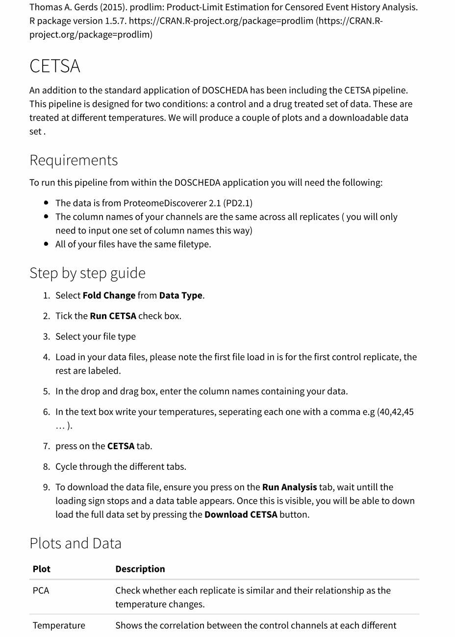
CETSAAn addition to the standard application of DOSCHEDA has been including the CETSA pipeline.This pipeline is designed for two conditions: a control and a drug treated set of data. These aretreated at different temperatures. We will produce a couple of plots and a downloadable dataset .

RequirementsTo run this pipeline from within the DOSCHEDA application you will need the following:

The data is from ProteomeDiscoverer 2.1 (PD2.1)The column names of your channels are the same across all replicates ( you will onlyneed to input one set of column names this way)All of your files have the same filetype.

Step by step guide1. Select Fold Change from Data Type.

2. Tick the Run CETSA check box.

3. Select your file type

4. Load in your data files, please note the first file load in is for the first control replicate, therest are labeled.

5. In the drop and drag box, enter the column names containing your data.

6. In the text box write your temperatures, seperating each one with a comma e.g (40,42,45… ).

7. press on the CETSA tab.

8. Cycle through the different tabs.

9. To download the data file, ensure you press on the Run Analysis tab, wait untill theloading sign stops and a data table appears. Once this is visible, you will be able to download the full data set by pressing the Download CETSA button.

Plots and DataPlot Description

PCA Check whether each replicate is similar and their relationship as thetemperature changes.

Temperature Shows the correlation between the control channels at each different

CorrelationControl

temperature and replicate.

TemperatureCorrelation Drug

Shows the correlation between the drug channels at each differenttemperature and replicate.

Protein Search Shows the protein profile for a selected protein.

The downloadable data is an excel sheet with three different sheets:

Sheet Description

Only_IC50_shift The value and associated p-values for the IC50 shift

IC50&bottom_shift The value and associated p-values for the IC50 and the bottom parametershift

Failed_to_model Gives a list of the failed proteins

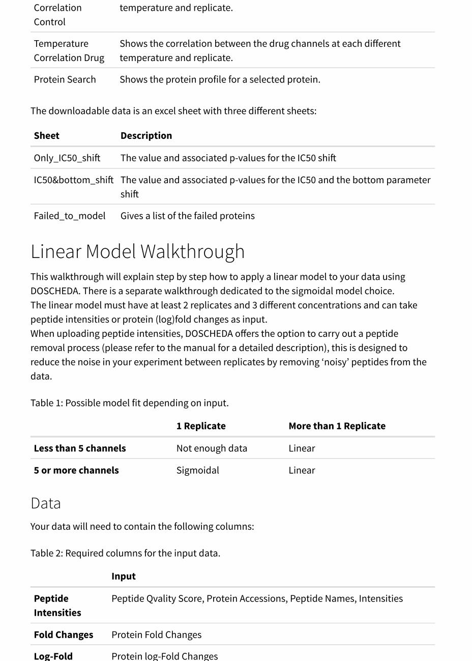
Linear Model WalkthroughThis walkthrough will explain step by step how to apply a linear model to your data usingDOSCHEDA. There is a separate walkthrough dedicated to the sigmoidal model choice.The linear model must have at least 2 replicates and 3 different concentrations and can takepeptide intensities or protein (log)fold changes as input.When uploading peptide intensities, DOSCHEDA offers the option to carry out a peptideremoval process (please refer to the manual for a detailed description), this is designed toreduce the noise in your experiment between replicates by removing ‘noisy’ peptides from thedata.

Table 1: Possible model fit depending on input.

1 Replicate More than 1 Replicate

Less than 5 channels Not enough data Linear

5 or more channels Sigmoidal Linear

DataYour data will need to contain the following columns:

Table 2: Required columns for the input data.

Input

PeptideIntensities

Peptide Qvality Score, Protein Accessions, Peptide Names, Intensities

Fold Changes Protein Fold Changes

Log-Fold Protein log-Fold Changes

Log-FoldChanges

Protein log-Fold Changes

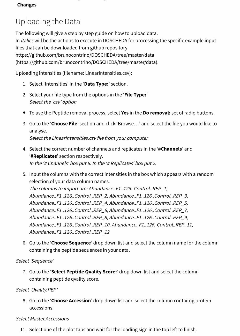
Uploading the DataThe following will give a step by step guide on how to upload data.In italics will be the actions to execute in DOSCHEDA for processing the specific example inputfiles that can be downloaded from github repositoryhttps://github.com/brunocontrino/DOSCHEDA/tree/master/data(https://github.com/brunocontrino/DOSCHEDA/tree/master/data).

Uploading intensities (filename: LinearIntensities.csv):

1. Select ‘Intensities’ in the ‘Data Type:’ section.

2. Select your file type from the options in the ‘File Type:’Select the ‘csv’ option

To use the Peptide removal process, select Yes in the Do removal: set of radio buttons.

3. Go to the ‘Choose File’ section and click ‘Browse…’ and select the file you would like toanalyse.Select the LinearIntensities.csv file from your computer

4. Select the correct number of channels and replicates in the ‘#Channels’ and‘#Replicates’ section respectively.In the ‘# Channels’ box put 6. In the ‘# Replicates’ box put 2.

5. Input the columns with the correct intensities in the box which appears with a randomselection of your data column names.The columns to import are: Abundance..F1..126..Control..REP_1,Abundance..F1..126..Control..REP_2, Abundance..F1..126..Control..REP_3,Abundance..F1..126..Control..REP_4, Abundance..F1..126..Control..REP_5,Abundance..F1..126..Control..REP_6, Abundance..F1..126..Control..REP_7,Abundance..F1..126..Control..REP_8, Abundance..F1..126..Control..REP_9,Abundance..F1..126..Control..REP_10, Abundance..F1..126..Control..REP_11,Abundance..F1..126..Control..REP_12

6. Go to the ‘Choose Sequence’ drop down list and select the column name for the columncontaining the peptide sequences in your data.

Select ‘Sequence’

7. Go to the ‘Select Peptide Qvality Score:’ drop down list and select the columncontaining peptide qvality score.

Select ‘Qvality.PEP’

8. Go to the ‘Choose Accession’ drop down list and select the column contaitng proteinaccessions.

Select Master.Accessions

11. Select one of the plot tabs and wait for the loading sign in the top left to finish.

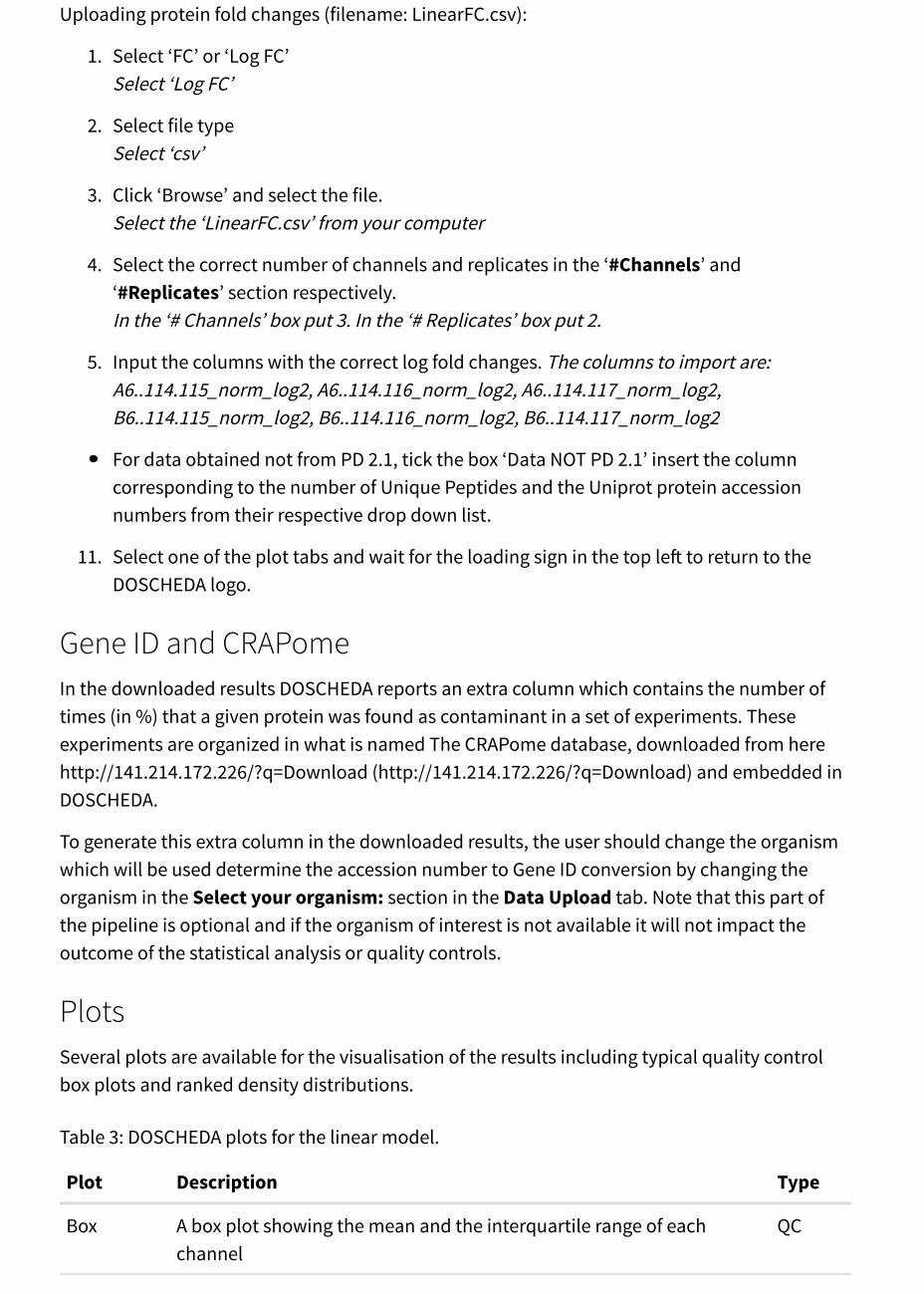
Uploading protein fold changes (filename: LinearFC.csv):

1. Select ‘FC’ or ‘Log FC’Select ‘Log FC’

2. Select file typeSelect ‘csv’

3. Click ‘Browse’ and select the file.Select the ‘LinearFC.csv’ from your computer

4. Select the correct number of channels and replicates in the ‘#Channels’ and‘#Replicates’ section respectively.In the ‘# Channels’ box put 3. In the ‘# Replicates’ box put 2.

5. Input the columns with the correct log fold changes. The columns to import are:A6..114.115_norm_log2, A6..114.116_norm_log2, A6..114.117_norm_log2,B6..114.115_norm_log2, B6..114.116_norm_log2, B6..114.117_norm_log2

For data obtained not from PD 2.1, tick the box ‘Data NOT PD 2.1’ insert the columncorresponding to the number of Unique Peptides and the Uniprot protein accessionnumbers from their respective drop down list.

11. Select one of the plot tabs and wait for the loading sign in the top left to return to theDOSCHEDA logo.

Gene ID and CRAPomeIn the downloaded results DOSCHEDA reports an extra column which contains the number oftimes (in %) that a given protein was found as contaminant in a set of experiments. Theseexperiments are organized in what is named The CRAPome database, downloaded from herehttp://141.214.172.226/?q=Download (http://141.214.172.226/?q=Download) and embedded inDOSCHEDA.

To generate this extra column in the downloaded results, the user should change the organismwhich will be used determine the accession number to Gene ID conversion by changing theorganism in the Select your organism: section in the Data Upload tab. Note that this part ofthe pipeline is optional and if the organism of interest is not available it will not impact theoutcome of the statistical analysis or quality controls.

PlotsSeveral plots are available for the visualisation of the results including typical quality controlbox plots and ranked density distributions.

Table 3: DOSCHEDA plots for the linear model.

Plot Description Type

Box A box plot showing the mean and the interquartile range of eachchannel

QC

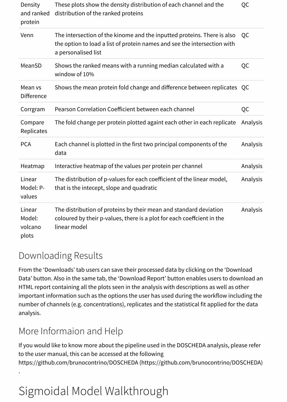
Densityand rankedprotein

These plots show the density distribution of each channel and thedistribution of the ranked proteins

QC

Venn The intersection of the kinome and the inputted proteins. There is alsothe option to load a list of protein names and see the intersection witha personalised list

QC

MeanSD Shows the ranked means with a running median calculated with awindow of 10%

QC

Mean vsDifference

Shows the mean protein fold change and difference between replicates QC

Corrgram Pearson Correlation Coefficient between each channel QC

CompareReplicates

The fold change per protein plotted againt each other in each replicate Analysis

PCA Each channel is plotted in the first two principal components of thedata

Analysis

Heatmap Interactive heatmap of the values per protein per channel Analysis

LinearModel: P-values

The distribution of p-values for each coefficient of the linear model,that is the intecept, slope and quadratic

Analysis

LinearModel:volcanoplots

The distribution of proteins by their mean and standard deviationcoloured by their p-values, there is a plot for each coeffcient in thelinear model

Analysis

Downloading ResultsFrom the ‘Downloads’ tab users can save their processed data by clicking on the ‘DownloadData’ button. Also in the same tab, the ‘Download Report’ button enables users to download anHTML report containing all the plots seen in the analysis with descriptions as well as otherimportant information such as the options the user has used during the workflow including thenumber of channels (e.g. concentrations), replicates and the statistical fit applied for the dataanalysis.

More Informaion and HelpIf you would like to know more about the pipeline used in the DOSCHEDA analysis, please referto the user manual, this can be accessed at the followinghttps://github.com/brunocontrino/DOSCHEDA (https://github.com/brunocontrino/DOSCHEDA).

Sigmoidal Model Walkthrough

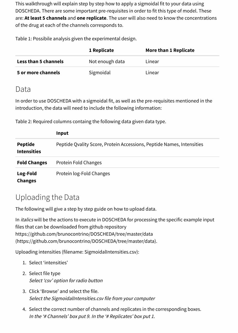
This walkthrough will explain step by step how to apply a sigmoidal fit to your data usingDOSCHEDA. There are some important pre-requisites in order to fit this type of model. Theseare: At least 5 channels and one replicate. The user will also need to know the concentrationsof the drug at each of the channels corresponds to.

Table 1: Possibile analysis given the experimental design.

1 Replicate More than 1 Replicate

Less than 5 channels Not enough data Linear

5 or more channels Sigmoidal Linear

DataIn order to use DOSCHEDA with a sigmoidal fit, as well as the pre-requisites mentioned in theintroduction, the data will need to include the following information:

Table 2: Required columns containg the following data given data type.

Input

PeptideIntensities

Peptide Qvality Score, Protein Accessions, Peptide Names, Intensities

Fold Changes Protein Fold Changes

Log-FoldChanges

Protein log-Fold Changes

Uploading the DataThe following will give a step by step guide on how to upload data.

In italics will be the actions to execute in DOSCHEDA for processing the specific example inputfiles that can be downloaded from github repositoryhttps://github.com/brunocontrino/DOSCHEDA/tree/master/data(https://github.com/brunocontrino/DOSCHEDA/tree/master/data).

Uploading intensities (filename: SigmoidalIntensities.csv):

1. Select ‘intensities’

2. Select file typeSelect ‘csv’ option for radio button

3. Click ‘Browse’ and select the file.Select the SigmoidalIntensities.csv file from your computer

4. Select the correct number of channels and replicates in the corresponding boxes.In the ‘# Channels’ box put 9. In the ‘# Replicates’ box put 1.

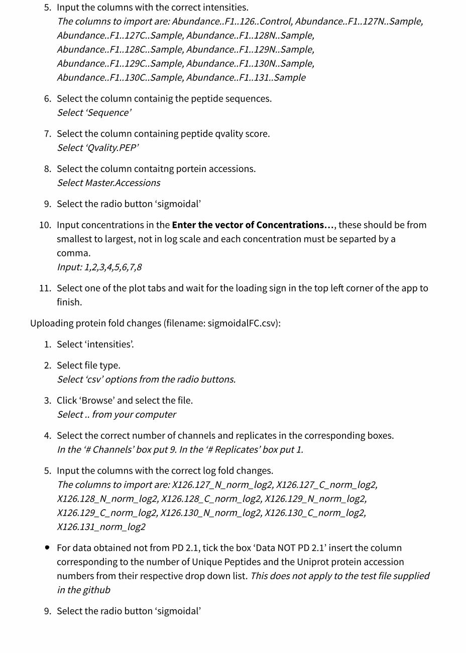
5. Input the columns with the correct intensities.The columns to import are: Abundance..F1..126..Control, Abundance..F1..127N..Sample,Abundance..F1..127C..Sample, Abundance..F1..128N..Sample,Abundance..F1..128C..Sample, Abundance..F1..129N..Sample,Abundance..F1..129C..Sample, Abundance..F1..130N..Sample,Abundance..F1..130C..Sample, Abundance..F1..131..Sample

6. Select the column containig the peptide sequences.Select ‘Sequence’

7. Select the column containing peptide qvality score.Select ‘Qvality.PEP’

8. Select the column contaitng portein accessions.Select Master.Accessions

9. Select the radio button ‘sigmoidal’

10. Input concentrations in the Enter the vector of Concentrations…, these should be fromsmallest to largest, not in log scale and each concentration must be separted by acomma.Input: 1,2,3,4,5,6,7,8

11. Select one of the plot tabs and wait for the loading sign in the top left corner of the app tofinish.

Uploading protein fold changes (filename: sigmoidalFC.csv):

1. Select ‘intensities’.

2. Select file type.Select ‘csv’ options from the radio buttons.

3. Click ‘Browse’ and select the file.Select .. from your computer

4. Select the correct number of channels and replicates in the corresponding boxes.In the ‘# Channels’ box put 9. In the ‘# Replicates’ box put 1.

5. Input the columns with the correct log fold changes.The columns to import are: X126.127_N_norm_log2, X126.127_C_norm_log2,X126.128_N_norm_log2, X126.128_C_norm_log2, X126.129_N_norm_log2,X126.129_C_norm_log2, X126.130_N_norm_log2, X126.130_C_norm_log2,X126.131_norm_log2

For data obtained not from PD 2.1, tick the box ‘Data NOT PD 2.1’ insert the columncorresponding to the number of Unique Peptides and the Uniprot protein accessionnumbers from their respective drop down list. This does not apply to the test file suppliedin the github

9. Select the radio button ‘sigmoidal’

10. Input concentrations in the Enter the vector of Concentrations…, these should be fromsmallest to largest, not in log scale and each concentration must be separted by acomma.Input: 1,2,3,4,5,6,7,8,9

11. Select one of the plot tabs and wait for the loading sign in the top left to finish.

GeneID and CRAPomeTo generate this extra column in the downloaded results, the user should change the organismwhich will be used determine the accession number to Gene ID conversion by changing theorganism in the Select your organism: section in the Data Upload tab. Note that this part ofthe pipeline is optional and if the organism of interest is not available it will not impact theoutcome of the statistical analysis or quality controls.

PlotsSeveral plots are available for the visualisation of the results including typical quality controlbox plots and ranked density distributions.

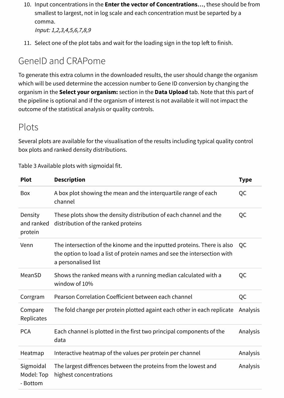
Table 3 Available plots with sigmoidal fit.

Plot Description Type

Box A box plot showing the mean and the interquartile range of eachchannel

QC

Densityand rankedprotein

These plots show the density distribution of each channel and thedistribution of the ranked proteins

QC

Venn The intersection of the kinome and the inputted proteins. There is alsothe option to load a list of protein names and see the intersection witha personalised list

QC

MeanSD Shows the ranked means with a running median calculated with awindow of 10%

QC

Corrgram Pearson Correlation Coefficient between each channel QC

CompareReplicates

The fold change per protein plotted againt each other in each replicate Analysis

PCA Each channel is plotted in the first two principal components of thedata

Analysis

Heatmap Interactive heatmap of the values per protein per channel Analysis

SigmoidalModel: Top- Bottom

The largest diffrences between the proteins from the lowest andhighest concentrations

Analysis

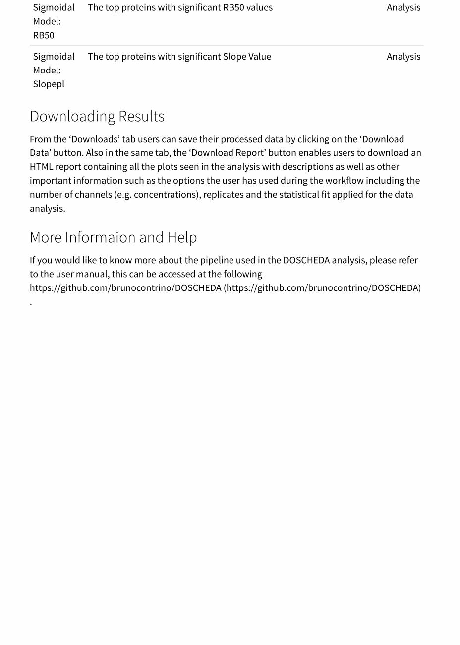
SigmoidalModel:RB50

The top proteins with significant RB50 values Analysis

SigmoidalModel:Slopepl

The top proteins with significant Slope Value Analysis

Downloading ResultsFrom the ‘Downloads’ tab users can save their processed data by clicking on the ‘DownloadData’ button. Also in the same tab, the ‘Download Report’ button enables users to download anHTML report containing all the plots seen in the analysis with descriptions as well as otherimportant information such as the options the user has used during the workflow including thenumber of channels (e.g. concentrations), replicates and the statistical fit applied for the dataanalysis.

More Informaion and HelpIf you would like to know more about the pipeline used in the DOSCHEDA analysis, please referto the user manual, this can be accessed at the followinghttps://github.com/brunocontrino/DOSCHEDA (https://github.com/brunocontrino/DOSCHEDA).