Embed Size (px)
Citation preview
Does Piped Water Reduce Diarrhea
for Children in Rural India?
Jyotsna Jalan and Martin Ravallion1
Indian Statistical Institute and World Bank
August 2001
Abstract: The impacts of public investments that directly improve children’s health are theoretically
ambiguous given that the outcomes also depend on parentally-provided inputs. Using propensity
score matching methods, we find that the prevalence and duration of diarrhea among children under
five in rural India are significantly lower on average for families with piped water than for
observationally identical households without piped water. However, our results indicate that the
health gains largely by-pass children in poor families, particularly when the mother is poorly
educated. Our findings point to the importance of combining infrastructure investments with
effective public action to promote health knowledge and income poverty reduction.
1 These are the views of the authors and should not be attributed to their employers, including the World Bank. We thank the National Council of Applied Economic Research for allowing us the use of their data, and the World Bank’s South Asia Poverty Reduction and Economic Management Group for their support. We are also grateful to Alok Bhargava, John Briscoe, Valerie Kozel, Mead Over, Jennifer Sara, Arijit Sen, Dominique van de Walle, seminar participants at the World Bank.
2
1. Introduction
The World Health Organization estimates that four million children under the age of five die
each year from diarrhea, mainly in developing countries.2 Unsafe drinking water is widely thought to
be a major cause, and this has motivated public programs to expand piped water access.
In this paper, we estimate the impacts on child health of piped water in a developing country.
We argue that expanding piped water is not a sufficient condition to improve child health status in
this setting. The source of ambiguity lies in the uncertainty about how public and private inputs
interact in the production of health conditional on the heterogeneous quality of public inputs.
The private inputs relevant to diarrhea prevalence and duration include hygienic water
storage, boiling water, oral re-hydration therapy, medical treatment, sanitation and nutrition. With the
right combination of these public and private inputs, diarrhoeal disease is almost entirely preventable.
However, behavior is known to play an important role. Public inputs such as access to a piped water
network can either displace parentally chosen private inputs or be complementary to them. Even
when there are child-health benefits (factoring in parental spending effects) the gains could well by-
pass children in poor families, taking account of parental behavioral responses to poverty.
For example, if piped water increases the marginal health benefit for parents of spending
more on their children’s health, and such spending is a normal good, then the health gains from piped
water will tend to rise with income. This is not implausible on a priori grounds. Piped water in rural
areas of developing countries is no doubt safer than many alternative sources, but it is often the case
that it still needs to be boiled or filtered and stored properly to be safe to drink. This can be a burden
for a poor family; a poor, or poorly educated mother may reasonably think that there are better uses
of time and money needed to provide this complementary input to piped water.
2 http://www.who.int/aboutwho/en/preventing/diarrhoeal.htm
3
It is plausible that there are private inputs that are cooperant with piped water in determining
child health. However, it can also be argued that such private inputs have positive income effects in
this setting, and there is supportive evidence. For example, it is estimated that 29% of the poorest
quintile (in terms of a composite wealth index) of families in rural India in 1992/93 used oral
rehydration therapy when a child had diarrhea, as compared to 50% in the richest quintile (Gwatkin
et al., 2000). Similarly, 52% of those in the poorest quintile sought medical treatment, as compared
to 78% in the richest.
The upshot of all this is that being connected to a piped water network may well be of limited
relevance to the poor from an epidemiological standpoint. Income poverty and lack of education and
knowledge may well constrain the potential health gains from water infrastructure improvements.
The incidence of health gains need not favor children from poor families even when facility
placement is pro-poor.
This paper looks for evidence of child-health gains from access to piped water. We use a
large, representative cross-sectional survey for rural India implemented in 1993-94. India
undoubtedly accounts for more child deaths due to unsafe water than any other single country. Parikh
et al. (1999) quote an estimate of 1.5 million child deaths per year in India due to diarrhea and other
diseases related to poor water quality. Moreover, estimates indicate that one fifth of the population of
rural India do not have access to safe drinking water (World Bank, 2000). Expanding access to piped
water is considered an important development action in India.
Our aim is not to model the effect of contaminated water on child health in this setting.
Rather we attempt to quantify the child health gains in terms of diarrhoeal disease from policy
interventions that expand access to piped water, and to see how the gains vary with household
circumstances, notably income and education. The main questions we ask are: Is a child less
vulnerable to diarrhoeal disease if he/she lives in a household with access to piped water? Do
4
children in poor, or poorly educated, households realize the same health gains from piped water as
others? Does income matter independently of parental education?
The following section establishes the theoretical ambiguity in the effect of access to piped
water on child health. Section 3 discusses the methodology we propose to test for child health gains
from piped water. Section 4 describes our data for rural India. The results are given in section 5,
while section 6 concludes.
2. A behavioral model of child health
We examine the impact on child health of an exogenous increase in access to piped water,
allowing for parental responses in the provision of other inputs to child health. The increase in
access could arise from an extension of the piped-water network into a community that had relied
previously on a well or stream. We show that once one allows for privately provided health inputs,
and assuming that parents care about more than just their children’s health, even the direction of the
effect on children’s health is theoretically ambiguous, and becomes an empirical question.
Let the health status (h) of a child depend on its access to piped water (w), parental spending
(s) on private inputs to child health, and a vector of personal and environmental characteristics (x).
The latter could include parental education, which could well enter non-separably with w; for
example, a well-educated mother knows how to make piped water safe to drink and how to treat
illnesses such as diarrhea. The health production function for the i’th child is:
),,( iiii xwsh h = (1)
The function h is assumed to be strictly increasing and twice differentiable in both s and w and to be
at least weakly concave in s (ruling out increasing returns to s). While w is likely to be a discrete
variable, for analytic convenience we treat it as a continuous variable in this section.
In choosing the level of private spending on child health, the family takes account of its lost
opportunity for consumption of other private goods , treated as a composite. We assume that spending
5
on child health has no intrinsic value to parents beyond its contribution to child health. However,
access to piped water also raises parental welfare. For example, having piped water reduces the time
spent collecting water from a well or stream. Exogenous income is y and sy − is left for parents’
consumption after deducting purchased inputs to child health. This gives parents utility
),,( xwsy u − in which the function u is strictly increasing and concave in sy − and strictly
increasing in w. Child health matters directly to parental welfare, but separably to their utility from
consumption. Thus the level of s is chosen by parents to maximize:
),,(),,( xwshxwsyu +− (2)
The solution equates the marginal impact of spending on child health with the marginal utility of own
consumption, ),,(),,( xwshxwsyu sy =− (using subscripts to denote partial derivatives), which can
also be written as:
),,( xyws s = (3)
This yields a maximum utility to parents of:
≡),,( xywv ),,( xywH + ],),,,([ xwxywsyu − (4)
where child health when parental inputs are optimal is given by:
],),,,([),,( xwxywshxywH = (5)
By the envelope theorem, ),,( xywv must be increasing in w. However, this need not hold for both
the components of parental utility. The effect of w on child health in a neighborhood of the
equilibrium in which private inputs are optimal is given by:
wwsw hshH += (6)
where:
yyss
swyww uh
hu s
+
−= (7)
6
It can be seen that ws has the same sign as ywsw uh − which could be positive, negative or zero.
Since the direct health effect is positive ( 0>wh ), it can be seen from (6) that 0≥− ywsw uh is
sufficient for piped water to improve child health.
Now consider the income effect on the health gain from piped water. This is given by:
wyssswswywy shhshsH ++= )( (8)
where
1≤+
=<yyss
yyy uh
u s0 (9)
In the special case in which there are no interaction effects in parental utility between piped water
and income or spending on child health ( 0== ywsw uh ), we find that 0=wyH ; the child health gain
from piped water is independent of household income. More generally however the direction of the
income effect could go either way. Consider the case in which parental direct utility is additively
separable between consumption and piped water ( 0=ywu ) and piped water does not alter the
marginal propensity to spend on private inputs to child health ( 0=yws ). Then swywy hsH 2= (using
(7) and (9)). So in this special case, the child health benefit from piped water will increase (decrease)
with income if the piped water is a complement (substitute) for the private inputs.
So far we have taken piped-water placement to be exogenous. In the empirical work we will
allow placement to be a function of a wide range of observable characteristics at household and
village level. Here we can think (quite generally) of the placement as maximizing some weighted
sum of ),,( iii yxwv over all i, with weights determined by a vector of characteristics of the
individual and his or her socio-political environment. (This might also include any variables
affecting the costs of service provision.) The solutions take the form ),( λii xww = where λ denotes
one or more multipliers on the constrain ts, including on resources available for providing the public
7
inputs. The task of the empirical work is then to measure the welfare gains from higher w,
recognizing that the observed levels of w in the cross-sectional data reflect purposive placement,
assuming that the relevant x’s are observable.
3. Identifying health impacts in cross-sectional data
We use propensity-score matching (PSM) methods to estimate the causal effects of piped
water on child health in a cross-sectional sample without random placement. PSM balances the
distributions of observed covariates between a treatment group and a control group based on
similarity of their predicted probabilities of having a given facility (their “propensity scores”). The
method does not require a parametric model linking facility placement to outcomes, and thus allows
estimation of mean impacts (including impacts conditional on income, for example) without arbitrary
assumptions about functional forms and error distributions. We exploit this flexibility to test for the
presence of potentially complex interaction effects as discussed in theoretical terms in the last
section. In this section we first outline the method, and then summarize its differences with other
methods found in the literature.
3.1 Propensity score matching
Two groups are identified: those households that have piped water (denoted Di =1 for
household i) and those that do not (Di=0). Units with piped water (the “treated” group) are matched
to households without (control group) on the basis of the propensity score:
P(xi) = Prob(Di =1| xi) (0< P(xi)<1) (10)
where xi is a vector of pre-exposure control variables. It is known from Rosenbaum and Rubin (1983)
that if (i) the Di’s are independent over all i, and (ii) outcomes are independent of participation given
xi, then outcomes are also independent of participation given P(xi), just as they would be if
8
participation were assigned randomly. 3 PSM uses P(x) (or a monotone function of P(x)) to select
controls for each of those treated. Exact matching on P(x) implies that the resulting matched control
and treated subjects have the same distribution of the covariates. PSM thus eliminates bias in
estimated treatment effects due to observable heterogeneity.
In practice the propensity score must be estimated. Here we follow the common practice in
PSM applications of using the predicted values from standard logit models to estimate the propensity
score for each observation in the participant and the comparison-group samples.4 Using the estimated
propensity scores, )(ˆ xP , matched-pairs are constructed on the basis of how close the scores are
across the two samples. The nearest neighbor to the i’th participant is defined as the non-participant
that minimizes [p(xi)- p(xj )]2 over all j in the set of non-participants, where p(xk) is the predicted odds
ratio for observation k i.e., p(xk)= )(ˆkxP /(1- )(ˆ
kxP ). Matches were only accepted if [p(xi)- p(xj )]2
was less than 0.001 (an absolute difference in odds less than 0.032).5
Letting jH∆ denote the gain in health status for the j’th child attributable to access to piped
water, the estimator of mean impact is:
∑∑==
=∆C
iijij
T
jjj hWh H
10
11 ) - (ω (11)
where hj1 is the post-intervention health indicator, hij0 is the outcome indicator of the ith non-treated
matched to the jth treated, T is the total number of treatments, C is the total number of non-treated
3 Assumption (ii) is sometimes referred to in the literature as the “conditional independence” assumption, and sometimes as “strong ignorability.” 4 Dehejia and Wahba (1999) report that their PSM results are robust to alternative estimators and alternative specifications for the logit regression. 5 We experimented with more stringent tolerance limits and the results were robust. However, with more stringent limits we also had to discard many more participants while calculating our impacts. Given that we already run into small sample problems for certain cells even with this tolerance limit when we categorize the sample on the basis of income and the level of female education (discussed later), we chose to report the results pertaining to a tolerance limit of 0.001.
9
households, ωj 's are the sampling weights used to construct the mean impact estimator, and the Wij’s
are the weights applied in calculating the average income of the matched non-participants.
Conditional mean impact estimators can be similarly defined by calculating equation (11) conditional
on observed characteristics. For example, comparing the conditional mean yH∆ across different
incomes y gives us a discrete estimator of the cross-partial derivative in equation (8).
There are several weights that one can use, ranging from “nearest neighbor” weights to non-
parametric weights based on kernel functions of the differences in scores (Heckman et al., 1997).6
We use the nearest five neighbors estimator, which takes the average outcome measure of the closest
five matched non-participants as the counter-factual for each participant.7
Following Rubin (1973) we also use a regression-adjusted estimator. This assumes a
conventional linear model for outcomes in the matched comparison group, 00 µβ += x h0 in obvious
notation. (The regression is only run for the matched comparison group, so it is not contaminated by
access to piped water.) The impact estimator in this case is then defined as:
∑∑==
−−=∆C
iiijij
T
jjjj xhW - xh H
100
101 )]ˆ()ˆ[( ββω (12)
where 0β̂ is the OLS estimate for the comparison group sample. 3.3 Other non-experimental methods
When feasible, pure randomization clearly dominates non-experimental methods such as
PSM. Unlike randomization, PSM still requires the conditional independence assumption (such that
participation and outcomes are independent given x). How does PSM compare to commonly used
non-experimental methods in this context?
6 Jalan and Ravallion (2000b) discuss the choice further, and find that their results for estimating income gains from an anti-poverty program are reasonably robust to the choice. 7 Rubin and Thomas (2000) use simulations to compare the bias in using the nearest five neighbors to just the nearest neighbor; no clear pattern emerges.
10
There are two main methods of assessing infrastructure impacts found in the literature. The
first is to compare average outcome indicators between villages (or other geographic units) that have
the facility and those that do not. Past methods of assessing health gains from water and sanitation
have often compared villages with piped water and those without (Esrey et al., 1991, review
numerous studies). The outcome indic ators have sometimes been at village level and sometimes at
household or individual level. Diverse methods have been used to control for heterogeneity; in some
cases no controls are used, but often some form of matched comparison is made. Clearly failure to
control for differences in village characteristics could severely bias such comparisons. Unlike some
commonly used matching estimates, PSM at village level would optimally balance the observed
covariates. To the extent that there is heterogeneity within villages, the aggregation could make it
hard to identify impact. Against this effect, aggregation to village level may well reduce
measurement error or household-specific selection bias. Moreover, since typically available village-
level data are less comprehensive than individual survey-based data, village-level matching will be
prone to greater bias due to unobserved covariates. We will compare our results using individual
PSM versus village PSM.
The second method found in the literature is to run a regression of the outcome indicators on
dummy variables for facility placement, allowing for the observable covariates entering as linear
controls.8 The widely used OLS regression method requires the same conditional independence
assumption as PSM, but they also impose (typically arbitrary) functional form assumptions
concerning the treatment effects and the control variables. Interaction effects have sometimes been
allowed; for example, Merrick (1985) included interactions between piped water and income and
education in regressions for child mortality in Brazil.
8 Early examples include Rosenzweig and Wolpin (1982), Wolfe and Behrman (1982) and Merrick (1985); recent examples include Lavy et al. (1996), Hughes and Dunleavy (2000) and Wagstaff (2000). Strauss and Thomas (1995) survey the large literature following this approach in studying health outcomes in micro data.
11
A variation on this second method is to use an instrumental variables estimator (IVE) treating
placement as endogenous. This method does not avoid an untestable conditional independence
assumption; in the case of IVE this is the exclusion restriction that the instrumental variable is
independent of outcomes given participation. And again the validity of causal inferences rests on the
ad hoc functional form assumptions required by standard (parametric ) IVE. Under these assumptions,
IVE identifies the causal effect robustly to unobserved heterogeneity.
The validity of the exclusion restriction required by IVE is questionable with only a single
cross-sectional data set; while one can imagine many variables that are correlated with placement,
such as geographic characteristics of an area, it is questionable on a priori grounds that those
variables are uncorrelated with outcomes given placement. There is more potential for identification
with longitudina l (panel) data, using methods that allow for latent (household and geographic)
heterogeneity (Rosenzweig and Wolpin, 1986; Pitt et al., 1995; Jalan and Ravallion, 2000a).
PSM also differs from commonly-used regression methods with respect to the sample used.
In PSM one confines attention to the matched sub-samples; unmatched comparison units are
dropped. By contrast, the regression methods commonly found in the literature use the full sample.
The simulations in Rubin and Thomas (2000) indicate that impact estimates based on full
(unmatched) samples are generally more biased, and less robust to miss-specification of the
regression function, than those based on matched samples.
A further difference relates to the choice of control variables. In the standard regression-
based method one naturally looks for predictors of the outcome measure, and preference is usually
given to variables that one can argue are exogenous to outcomes. In PSM one is looking instead for
covariates of participation, possibly including variables that are poor predictors of outcomes. Indeed,
analytic results and simulations indicate that variables with weak predictive ability for outcomes can
still help reduce bias in estimating causal effects using PSM (Rubin and Thomas, 2000).
12
4. Data
We use a household survey conducted by India’s National Council of Applied Economic
Research in 1993-94. This is a nationally representative survey collecting detailed information on
education and health status of 33,000 rural households from 1765 villa ges covering 16 states of India.
Multi-stage sampling design was used where income from agriculture and rural female literacy rates
were the variables used to form homogeneous strata. From these strata a certain number of districts
were selected with proba bility of selection proportional to the rural population in the district. The
survey collected detailed information on health status of household members. The income survey
used 12 questions to arrive at a total income, comprising income from allied agricultural activities,
artisan/independent work, petty trade/small business, organized trade/business, salaried employment,
qualified profession, cattle tending, rent, interest, dividends, other sources, imputed income from
agriculture, annual income of the household from agricultural work and annual income of the
household from non-agricultural work.
We aim to measure the child-health effects of access to piped water. The latter is indicated by
whether the household reports access to piped water from a tap eit her inside or outside the house.
Applying the household weights in the data, 24.8% of households had piped water (7.6% inside the
house and 17.3% outside). The proportion of households with piped water varies little with income
(Table 1). In the main analysis we do not distinguish whether the tap is inside or outside the house,
on the grounds that this difference only matters to health outcomes via parental behavior, so the
difference is subsumed in studying the relationship between access to a piped water and child health.
However, it is still of interest to test for differences in impact according to whether the piped water is
a tap inside the house or a public tap, given the obvious possibilities for stored water contamination.
We provide such a test.
13
We examine impact on the prevalence of diarrhea among children under five years of age and
the reported illness duration. And we assess incidence against household income per person and by
the highest education level of any female in the household.
The sample includes 9,000 households with piped water and 24,000 without. Table 1 gives
sample sizes for those with piped water stratified by income and female education. Unlike standard
matching techniques we match "treatment" group with "non-treatment" group from the same
household survey. This means that standard requirements of getting better matches are easily met,
such as that treatment and counterfactual groups have the same questionnaire administered to them
and that they belong to the same economic environment.
5. Impact estimates
5.1 Estimated child-health impacts using PSM at household level
Table 2 reports the estimates of the logit regression where the binary outcome takes a value
one if the household has access to piped water and zero otherwise. The regressors comprised a wide
range of village and household characteristics including seemingly plausible proxies for otherwsie
omitted variables. The village variables included agricultural modernization, and measures of
educational and social infrastructure. The household variables included demographics, education,
religion, ethnicity, assets, housing conditions, and state dummy variables.
While we saw little sign of correlation between households with piped water and income in
Table 1, there are a number of significant explanatory variables of piped water placement in Table 2.
The results are generally unsurprising. Households living in larger villages (in terms of population),
villages with a high school, a “pucca” (“sealed”) road, a bus stop, a telephone, a bank, and a market
were more likely to have piped water. The probability of scheduled tribe (but not scheduled caste)
households having access to piped water was lower compared to the non-minority population.
Christian households were more likely to have access to piped water. Owning a home made it less
14
probable; this is unlikely to be a (perverse) wealth effect, but to be related to the fact that demand for
rental housing tends to come from relatively well-off people in rural India, and so this type of
housing tends to be better equipped. Other housing characteristics have the expected effects, such as
living in a pucca house and having electricity. Female -headed households are more likely to have
piped water. A positive wealth effect controlling for these other characteristics is indicated by the
fact that the more land one owns the greater the probability that one has access to piped water.
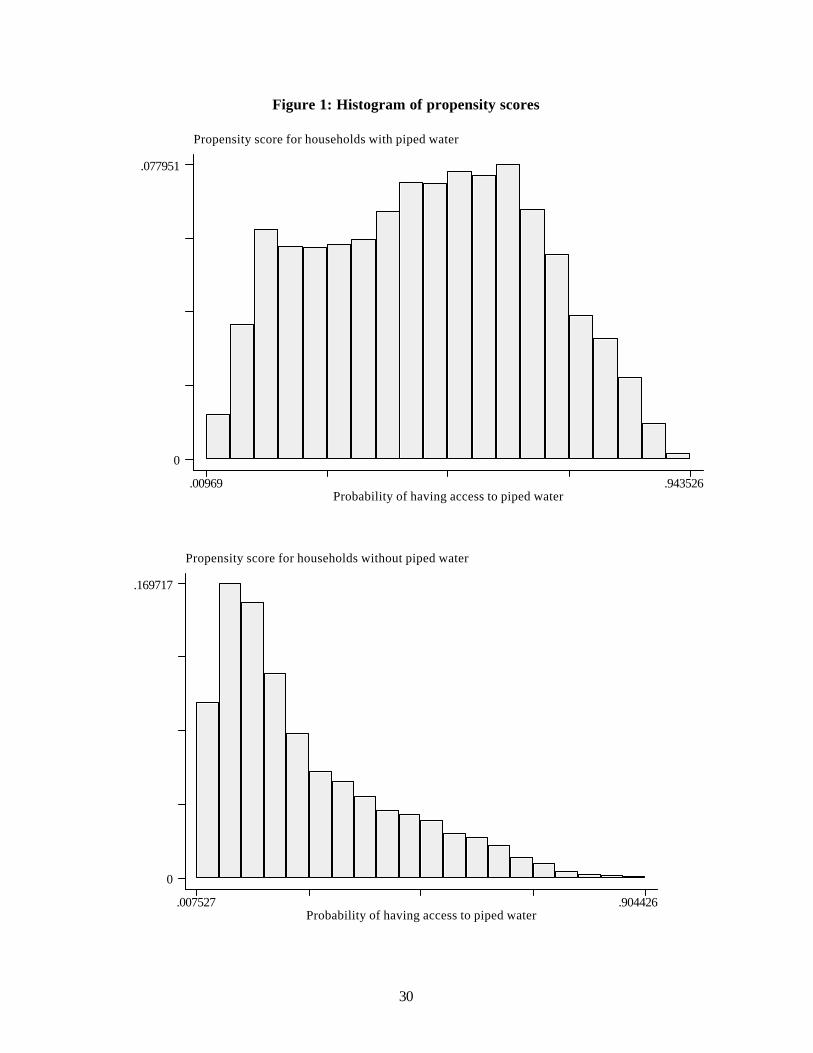
Prior to matching, the estimated propensity scores for those with and without piped water
were respectively 0.5495 (standard error of 0.285) and 0.1933 (0.184). Figure 1 reports the
histograms of the estimated propensity scores for the two groups. From the original sample, we lose
approximately 650 treatment households due to our inability to find a sufficiently good match. After
matching there was negligible difference in the mean propensity scores of the two groups (0.3743,
with a standard error of 0.189, for those with piped water versus 0.3742, with a standard error of
0.189, for the matched control group).
Table 3 reports descriptive statistics for the full sample of households with piped water as
well as when the sample is stratified by both income and the highest level of education among female
members. (Here and elsewhere we use the sampling weights provided in the data). The overall
prevalence of diarrhea is 1.1% in the sample, with an average of 0.33 days of illness and a mean
expenditure of 0.74 rupees per episode of diarrhea. Disease prevalence and length of illness fall with
higher income and education. For example, diarrhea prevalence amongst infants in families with
piped water is twice as high for those in the poorest quintile than the richest.
The estimated mean impacts on the child-health indicators are also given in Table 3. The
results for mean impact indicate that access to piped water significantly reduces diarrhea prevalence
and duration. Disease prevalence amongst those with piped water would be 21% higher without it.
Illness duration would be 29% higher. The regression-adjusted impact estimator (equation 12) gave
very similar results (using the full set of regressors in Table 2 as the x vector). The impact estimator

15
for diarrhea prevalence was –0.0023 (with a standard error of 0.053) and for diarrhea duration it was
–0.1005 (standard error of 0.021).
Once we stratify the sample by quintiles based on income per capita, we find no significant
child-health gains amongst the poorest two quintiles (roughly corresponding to the poor in India, by
widely used poverty lines). However, from the 40th quintile onwards there are very significant
impacts on child health in households with piped water. We see that the income gradient amongst
those with piped water is almost entirely attributable to piped water. For example, we can infer that
without piped water there would be no difference in infant diarrhea prevalence between the poorest
quintile and the richest. Health impacts from piped water tend to be larger and more significant in
families with better educated women. We found a similar pattern when we stratified instead by the
highest education of the household head.
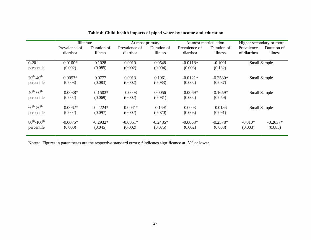
In Table 4 we report the joint effects of income and female education to test the hypothesis
that income and female education interact jointly with piped water in determining child health. When
we stratify by both income and education, we find that even in the bottom two quintiles, if a woman
in the household has more than primary school then the household extracts significant gains from
piped water in terms of lower preva lence and duration of diarrhea among children. However, these
gains are not visible if the highest level of education among female members in the household is at
most primary school. The effect of education is absent in the upper quintiles. Irrespective of the
education levels of the female members in the household, there are significant gains to child health
in households with access to piped water. These results suggest that among poorer households, the
education of women matters greatly to achieving the child-health benefits from piped water.
We have defined a household with piped water to be one with access either via a tap in the
premises of the household or from a public tap nearby. A concern with this broad definition is that
perhaps it disguises the differences in impacts of having the facility inside the house versus outside.
To test for such differences we analyze the sub-sample of households with access to either source of
16
piped water and compare the health outcomes (prevalence and duration of diarrhea) of children
among households with a tap in the household to those who rely on public tap to get drinking water.
Our results are reported in Tables 5 and 6.
There is little overall difference in the impact on the prevalence of diarrhea between
households with piped water inside the home versus those using a public tap (Table 5). However,
illness duration is nearly 40% higher in households where the source of drinking water is a public tap
rather than a tap within the household premises, suggesting less contamination due to storage and
hence less severe illness in the latter case.
We find a very strong differential impact of a private tap on both the duration and the
prevalence of diarrhea among households where the female member is uneducated. With some
education, however, there is no difference in the health outcomes of children across households
categorized on the basis of source of piped water. Finally, when we stratify the sample with respect
to income and education, we find that it is only among households where the female member is
illiterate that there are strong impacts of having the piped water source inside the household.
5.2 Village-level estimator
We compared the above results to village-level matching, as might be done with only village-
level data. For the purpose of comparison, we confine the matching to village-level data from a
village survey (not using village aggregates formed from the household data). Out of 1624 villages in
the sample, 324 had piped water. Far fewer control variables were available at village level; we
included 20 variables, instead of the 90 variables used for household -level matching. The control
variables for estimating the propensity score at village level were (log)village size, share of land
irrigated in gross cropped area, schools in the village, female to male student ratio, proportion of
people belonging to a scheduled caste/tribe, and (agricultural and non-agricultural) wages and prices
in the village. Only the wage rate variables were individually significant, though the LR test
17
indicated the explanatory variables were jointly significant and the pseudo-R2 was 0.2294. After
checking for common support, we could estimate impact for 262 villages against a matched control
group of nearest neighbors in terms of the propensity score. We used the nearest neighbor as opposed
to nearest five neighbors to match villages because it was difficult to find matches which satisfied
our tolerance limit criterion in terms of the metric distance between the propensity score ratios of the
treated and the controls for a large number of observations.
We found that diarrhea prevalence and duration were not significantly different in the
villages with piped water compared to the matched control villages. The impact estimates were
0.0012 for diarrhea prevalence and 0.1001 for duration and neither was significantly different from
zero at even the 10% level (standard errors of 0.024 and 0.1001 respectively).
6. Conclusions
It can be expected that parental choices about private inputs to child health will respond to
changes in the household environment. This has implications for understanding the incidence of
child-health benefits from local infrastructure development. Potential health benefits may not be
realized in practice. For example, there may be little benefit to children in poor families if private
inputs (with positive income effects) and public inputs have cooperant effects on health. Or the
incidence of child-health gains could be decidedly pro-poor if the private and public inputs are in fact
substitutes.
To investigate this issue we have used the propensity score matching method to quantify the
expected health gains to children from piped water, and to examine how those gains vary according
to income and education. This method is well suited to the present application since it allows a
flexible (nonparametric) description of the interaction effects with income and education. While the
method does not require ad hoc assumptions about the functional for m of impacts and exclusion
restrictions, it only eliminates selection bias due to observable differences between those with piped

18
water and those without it. While we have used a rich data, allowing us to match on a wide range of
characteristics, the possibility remains of latent factors correlated with both access to piped water and
child health.
We have estimated impacts on diarrhea prevalence and duration in children under five. We
find significantly lower prevalence and duration of the disease for children living in households with
piped water as compared to a comparison group of households matched on the basis of their
propensity scores. However, matching at village level instead does not indicate lower diarrhea
prevalence or duration.
There are striking differences in the child-health gains from piped water according to family
income and adult female education. While there are significant health gains overall from access to
piped water, we find no evidence of significant gains for the poorest 40% in terms of incomes.
Indeed, the income gradient in disease prevalence and duration is attributable to piped water; no
income effect is found for the matched control group. Health gains from piped water tend to be lower
for children with less well-educated women in the household. Here education is no doubt proxying
for knowledge about how to assure that water is safe to drink and how best to treat illness. The
income effect on the child-health benefits from piped water is also found at given levels of education,
though it is not as pronounced.
When we look at only the sub-sample of households with access to either source of piped
water and compare the prevalence and duration of diarrhea among children under five across
households with access from a tap inside the house versus access via a public tap we find two
striking effects: first the duration of illness is reduced significantly if households have drinking water
source within the premises. Second, the impact is greater in households where the female member is
illiterate.
A number of messages for policy emerge from this study. We confirm that there are
statistically significant, and quantitatively non-negligible, mean impacts of piped water on an
19
important aspect of child health. However, we also find that the average impact is a deceptive
indicator for inferring gains to children in poor families. Policy makers trying to reach children in
poor families—who are typically the most prone to disease—will need to do more that relying on
making facility placement pro-poor, such as by locating interventions in poor areas. The incidence of
health gains need not favor children from poor families even when placement favors the poor. The
evident weakness of the impacts we find amongst the income poor, and poorly educated, points to the
importance of combining public investments in this type of infrastructure with other interventions in
education and income-poverty reduction.
20
References
Dehejia, Rajeev H., and Sadek Wahba, 1999, “Causal Effects in Non-Experimental Studies: Re-
Evaluating the Evaluation of Training Programs”, Journal of the American Statistical
Association, 94: 1053-1062.
Esrey, S.A., J.B. Potash, L. Roberts, and C. Shiff, 1991, “Effects of Improved Water Supply and
Sanitation on Ascariasis, Diarrhoea, Dracunculiasis, Hookworm Infection, Schistosomiasis
and Trachoma,” Bulletin of the World Health Organization 69(5): 609-621.
Gwatkin, Davidson R., Shea Rustein, Kiersten Johnson, Rohini P. Pande and Adam Wagstaff, 2000,
“Socio-Economic Differences in Health, Nutrition, and Population in India,” World Bank.
http://www.worldbank.org/poverty/health/data/india/india.pdf
Heckman, J., H. Ichimura, and P. Todd, 1997, “Matching as an Econometric Evaluation Estimator:
Evidence from Evaluating a Job Training Programme”, Review of Economic Studies, 64: 605-
654.
Heckman, J., H. Ichimura, J. Smith, and P. Todd, 1998, “Characterizing Selection Bias using
Experimental Data”, Econometrica , 66: 1017-1099.
Hughes, Gordon and Meghan Dunleavy, 2000, “Why do Babies and Young Children Die in India?
The Role of the Household Environment,” mimeo, the World Bank and MCP Hahnemann
School of Medicine.
Jalan, Jyotsna and Martin Ravallion, 2000a, “Geographic Poverty Traps? A Micro Model of
Consumption Growth in Rural China,” mimeo, Development Research Group, World Bank.
Jalan, Jyotsna and Martin Ravallion, 2000b, “Estimating Benefit Incidence for an Anti-Poverty
Program Using Propensity Score Matching,” mimeo, Development Research Group, World
Bank.
21
Lavy, Victor, John Strauss, Duncan Thomas, and Philippe de Vreyer, 1996, “Quality of Health Care,
Survival and Health Outcomes in Ghana”, Journal of Health Economics 15: 333-357.
Merrick, Thomas W., 1985, “The Effect of Piped Water on Early Childhood Mortality in Urban
Brazil,” Demography 22(1): 1-24.
Parikh, Kirit S., Jyoti Parikh, and Tata L. Raghu Ram, 1999, “Air and Water Quality
Management: New Initiatives Needed” in Kirit S. Parikh (ed.) India Development Report
1999-2000, Oxford University Press.
Pitt, Mark, Mark Rosenzweig, and Donna Gibbons, 1995, "The Determinants and
Consequences of the Placement of Government Programs in Indonesia", in D. van
de Walle and K. Nead (eds) Public Spending and the Poor: Theory and Evidence ,
Baltimore: Johns Hopkins University Press for the World Bank.
Rosenbaum, P. and D. Rubin, 1983, “The Central Role of the Propensity Score in Observational
Studies for Causal Effects,” Biometrika, 70: 41-55.
Rosenzweig, Mark R. and K.I. Wolpin (1982), “Governmental Interventions and Household
Behavior in a Deve loping Country. Anticipated and Unanticipated Consequences of Social
Programs,” Journal of Development Economics 10: 209-225.
Rosenzweig, Mark R. and K.I. Wolpin (1986), "Evaluating the Effects of Optimally
Distributed Public Programs: Child Health and Fa mily Planning Interventions",
American Economic Review, 76: 470-82.
Rubin, Donald B. (1973), "The use of matched sampling and regression adjustment
to remove bias in observational studies" Biometrics, 29, 159-183.
Rubin, Donald B., and Neal Thomas (2000), “Combining Propensity Score Matching
with Additional Adjustments for Prognostic Covariates,” Journal of the American
Statistical Association 95: 573-585.
Strauss, John, and Duncan Thomas, 1995, “Human Resources: Empirical Modeling of
22
Household and Family Decisions,” in J. Behrman and T.N. Srinivasan (eds),
Handbook of Development Economics, Volume 3, Amsterdam: North-Holland.
Todd, Petra, 1995, “Matching and Local Linear Regression Approaches to Solving the Evaluation
Problem with a Semiparametric Propensit y Score”, mimeo, University of Chicago.
Wagstaff, Adam, 2000, “Unpacking the Causes of Inequalities in Child Survival: The Case of Cebu,
The Philippines,” Development Research Group, World Bank.
Wolfe, Barbara L., and Jere R. Behrman, 1982, “Determinants of Child Mortality,
Health and Nutrition in a Developing Country”, Journal of Development
Economics 11: 163-193.
Table 1: Access to piped water across the income distribution and by education
Households with piped water stratified by highest education of female members
Income quintiles (stratified by household income per person)
Number of observations
Percentage of people with piped water Illiterate At most
primary At most
matriculation Higher secondary
or more Full sample
Bottom 20th percentile 6581 27.18 768 655 251 33 1707 20th-40th percentile 6508 25.40 674 590 274 29 1567 40th-60th percentile 6543 26.96 667 560 371 60 1658 60th-80th percentile 6694 29.62 660 602 462 90 1814 Top 20th percentile 6904 33.63 665 593 638 185 2081 Full sample 33230 28.62 3434 3000 1996 397 8827
Table 2 Logit regression for piped water
Coefficient t-statistic Village variables
Village size (log) 0.08212 4.269 Proportion of gross cropped area which is irrigated: >0.75 -0.04824 -1.185 Proportion of gross cropped area which is irrigated: 0.5-0.75 0.19399 4.178 Whether village has a day care center -0.07249 -2.225 Whether village has a primary school -0.08136 -1.434 Whether village has a middle school -0.09019 -2.578 Whether village has a high school 0.26460 7.405 Female to male students in the village 0.10637 3.010 Female to male students for minority groups -0.07661 -2.111 Main approachable road to village: pucca road 0.19441 3.637 jeepable/kuchha road -0.00163 -0.033 Whether bus-stoop is within the village 0.11423 2.951 Whether railway station is within the village 0.00920 0.179 Whether there is a post-office within the village 0.02193 0.550 Whether the village has a telephone facility 0.33059 9.655 Whether there is a community TV center in the village 0.09859 2.661 Whether there is a library in the village -0.04153 -1.116 Whether there is a bank in the village 0.19084 4.655 Whether there is a market in the village 0.31690 6.092 Student teacher ratio in the village 0.00242 5.295
Household variables Whether household belongs to the Scheduled Tribe -0.21288 -4.203 Whether household belongs to the Scheduled Caste -0.01045 -0.288 Whether it is a Hindu household -0.24195 -1.709 Whether it is a Muslim household -0.21631 -1.427 Whether it is a Christian household 0.40367 2.426 Whether it is a Sikh household -0.86645 -4.531 Household size 0.00337 0.571 Utilization of landholdings: used for cultivation? 0.17109 1.914 Whether the house belongs to the household -0.18988 -2.854 Whether the household owns other property 0.00181 0.044 Whether the household has a bicycle -0.26514 -8.243 Whether the household has a sewing machine 0.01183 0.252 Whether the household owns a thresher -0.05790 -0.577 Whether the household owns a winnower 0.21842 1.820 Whether the household owns a bullock-cart -0.25900 -5.430 Whether the household owns a radio 0.01036 0.251 Whether the household owns a TV 0.08095 1.335 Whether the household owns a fan 0.01336 0.321 Whether the household owns any livestock -0.07780 -2.339 Nature of house: kuchha -0.10004 -2.775 Pucca 0.12039 2.709 Condition of house: good 0.00230 0.036 Livable 0.09268 1.756
25
Rooms in house: one -0.10771 -1.371 Two 0.06822 0.952 three to five 0.07514 1.112 Whether household has a separate kitchen -0.01993 -0.533 Whether the kitchen is ventilated 0.08103 2.212 Whether the household has electricity 0.40641 11.217 Occupation of the head: cultivator -0.02425 -0.481 agricultural wage labor 0.02432 0.429 Non-agricultural wage labor 0.14628 2.254 Self-employed -0.06921 -0.955 Whether male members listen to radio 0.20089 3.484 Whether female members listen to radio -0.12415 -2.177 Whether male members watch TV 0.09365 1.291 Whether female members watch TV 0.03863 0.493 Whether male members read newspapers 0.08950 1.813 Whether female members read newspapers -0.04066 -0.631 Proportion of household members who are 60+ -0.11370 -1.067 Proportion of females among adults 0.04646 0.331 Proportion of males among children 0.08436 0.779 Proportion of females among children 0.05498 0.498 Whether household head is male -0.18041 -2.321 Whether household head is single -0.16659 -1.268 Whether household head is married -0.02603 -0.422 Whether household head is illiterate -0.13048 -1.454 Whether household head is primary school educated -0.03694 -0.416 Whether household head is matriculation educated -0.03364 -0.385 Whether household head is higher secondary -0.05545 -0.475 Gross cropped area -0.00020 -0.666 Gross irrigated area -0.00050 -1.342 Landholding size: landless -0.32849 -3.996 marginal -0.31056 -3.987 small -0.22129 -2.916 Constant -1.49531 -5.396 Log-likelihood function -16236.565 Number of observations 33216 Notes: In addition to the above variables 15 dummies were included to control for state specific effects.
26
Table 3: Impacts of piped water on diarrhea prevalence and duration for children under five
Prevalence of diarrhea Duration of illness Mean for those
with piped water
(st.dev.)
Impact of piped water
(st.error)
Mean for those with piped
water (st.dev.)
Impact of piped water
(st.error)
Full sample
0.0108 (0.046)
-0.0023* (0.001)
0.3254 (1.650)
-0.0957* (0.021)
Stratified by household income per capita Bottom 20th percentile
0.0155 (0.055)
0.0032* (0.001)
0.4805 (2.030)
0.0713 (0.053)
20th-40th percentile
0.0136 (0.051)
0.0007 (0.001)
0.4170 (1.805)
0.0312 (0.051)
40th-60th percentile
0.0083 (0.038)
-0.0039* (0.001)
0.2636 (1.418)
-0.1258* (0.042)
60th -80th percentile
0.0100 (0.044)
-0.0036* (0.001)
0.3195 (1.703)
-0.1392* (0.048)
Top 20th percentile
0.0076 (0.042)
-0.0068* (0.001)
0.1848 (1.254)
-0.2682* (0.036)
Stratified by highest education level of a female member Illiterate
0.0131 (0.053)
-0.0000 (0.001)
0.3588 (1.710)
-0.0904* (0.036)
At most primary school educated
0.0112 (0.045)
-0.0015 (0.001)
0.3502 (1.739)
-0.0465 (0.036)
At most matriculation educated
0.0074 (0.038)
-0.0065* (0.001)
0.2573 (1.476)
-0.1708* (0.039)
Higher secondary or more
0.0050 (0.027)
-0.0080* (0.002)
0.1880 (1.158)
-0.2077* (0.076)
Notes: *indicates significance at the 5% level or lower
27
Table 4: Child-health impacts of piped water by income and education
Illiterate At most primary At most matriculation Higher secondary or more Prevalence of
diarrhea
Duration of illness
Prevalence of diarrhea
Duration of illness
Prevalence of diarrhea
Duration of illness
Prevalence of diarrhea
Duration of illness
0-20th percentile
0.0100* (0.002)
0.1028 (0.089)
0.0010 (0.002)
0.0548 (0.094)
-0.0118* (0.003)
-0.1091 (0.132)
Small Sample
20th-40th percentile
0.0057* (0.003)
0.0777 (0.083)
0.0013 (0.002)
0.1061 (0.083)
-0.0121* (0.002)
-0.2580* (0.087)
Small Sample
40th-60th percentile
-0.0038* (0.002)
-0.1503* (0.069)
-0.0008 (0.002)
0.0056 (0.081)
-0.0069* (0.002)
-0.1659* (0.059)
Small Sample
60th-80th percentile
-0.0062* (0.002)
-0.2224* (0.097)
-0.0041* (0.002)
-0.1691 (0.070)
0.0008 (0.003)
-0.0186 (0.091)
Small Sample
80th-100th percentile
-0.0075* (0.000)
-0.2932* (0.045)
-0.0051* (0.002)
-0.2435* (0.075)
-0.0063* (0.002)
-0.2578* (0.008)
-0.010* (0.003)
-0.2637* (0.085)
Notes: Figures in parentheses are the respective standard errors; *indicates significance at 5% or lower.
28
Table 5: Differential impacts of piped water inside the house (rather than outside) on diarrhea prevalence and duration for children under five
Prevalence of diarrhea Duration of illness
Mean for those with piped water
(st.dev.)
Impact of piped water inside the
house (st.error)
Mean for those with piped water
(st.dev.)
Impact of piped water inside the
house (st.error)
Full sample
0.0162 (0.058)
-0.0018 (0.002)
0.4865 (2.065)
-0.1991* (0.062)
Stratified by household income per capita
Bottom 20th percentile
0.0246 (0.069)
0.0027 (0.005)
0.7189 (2.555)
0.0499 (0.175)
20th-40th percentile
0.0207 (0.062)
0.0006 (0.004)
0.6825 (2.568)
-0.1577 (0.178)
40th-60th percentile
0.0132 (0.050)
-0.0055**
(0.003)
0.4907 (2.251)
-0.2849**
(0.172) 60th -80th percentile
0.0148 (0.053)
-0.0018 (0.003)
0.4647 (1.767)
-0.2360**
(0.126) Top 20th percentile
0.0113 (0.054)
-0.0035 (0.058)
0.2452 (1.307)
-0.2898* (0.082)
Stratified by highest education level of a female member
Illiterate
0.0208 (0.065)
-0.0051**
(0.003)
0.5711 (2.173)
-0.5060* (0.117)
At most primary school educated
0.0163 (0.056)
0.0007 (0.003)
0.6210 (2.541)
0.0565 (0.128)
At most matriculation educated
0.0102 (0.046)
-0.0015 (0.003)
0.2640 (1.252)
-0.1178 (0.076)
Higher secondary or more
0.0122 (0.053)
0.0031 (0.004)
0.2198 (1.078)
-0.0389 (0.107)
Notes: *indicates significance at the 5% level or lower, ** indicates significance between 5%-10%
29
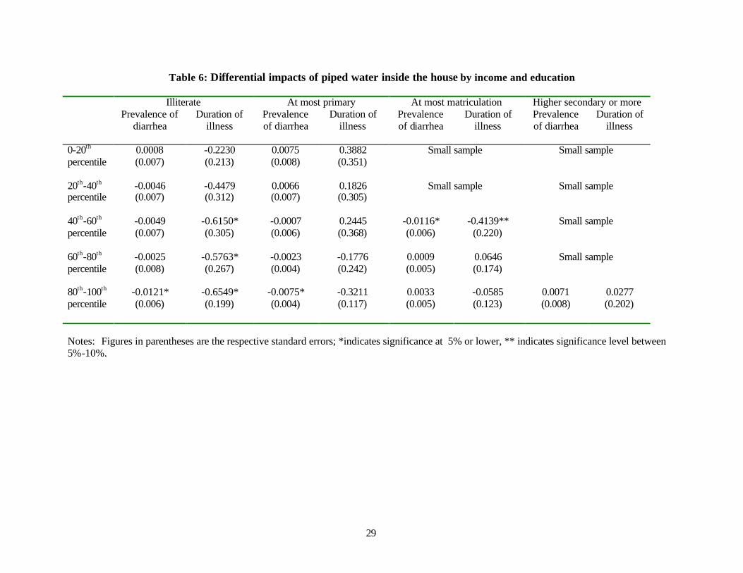
Table 6: Differential impacts of piped water inside the house by income and education
Illiterate At most primary At most matriculation Higher secondary or more Prevalence of
diarrhea
Duration of illness
Prevalence of diarrhea
Duration of illness
Prevalence of diarrhea
Duration of illness
Prevalence of diarrhea
Duration of illness
0-20th percentile
0.0008 (0.007)
-0.2230 (0.213)
0.0075 (0.008)
0.3882 (0.351)
Small sample
Small sample
20th-40th percentile
-0.0046 (0.007)
-0.4479 (0.312)
0.0066 (0.007)
0.1826 (0.305)
Small sample Small sample
40th-60th percentile
-0.0049 (0.007)
-0.6150* (0.305)
-0.0007 (0.006)
0.2445 (0.368)
-0.0116* (0.006)
-0.4139** (0.220)
Small sample
60th-80th percentile
-0.0025 (0.008)
-0.5763* (0.267)
-0.0023 (0.004)
-0.1776 (0.242)
0.0009 (0.005)
0.0646 (0.174)
Small sample
80th-100th percentile
-0.0121* (0.006)
-0.6549* (0.199)
-0.0075* (0.004)
-0.3211 (0.117)
0.0033 (0.005)
-0.0585 (0.123)
0.0071 (0.008)
0.0277 (0.202)
Notes: Figures in parentheses are the respective standard errors; *indicates significance at 5% or lower, ** indicates significance level between 5%-10%.
30
Figure 1: Histogram of propensity scores
Propensity score for households with piped water
Probability of having access to piped water.00969 .943526
0
.077951
Propensity score for households without piped water
Probability of having access to piped water.007527 .904426
0
.169717