Doctoral Dissertation Comparative Analysis of …...Doctoral Dissertation Comparative Analysis of Convergence on Regional Economic Integration: The Eurozone and ASEAN ZAENAL MUTAQIN

Doctoral Dissertation

Comparative Analysis of Convergence on Regional Economic Integration:

The Eurozone and ASEAN

ZAENAL MUTAQIN

Graduate School for International Development and Cooperation

Hiroshima University

September 2013



D102422

ZAENAL MUTAQIN

A Dissertation Submitted to

the Graduate School for International Development and Cooperation

of Hiroshima University in Partial Fulfillment

of the Requirement for the Degree of

Doctor of (Enter the name of your degree)

September 2013

iv

TABLE OF CONTENTS

Table of Contents ..................................................................................................................... iv

List of Tables ............................................................................................................................. x

Lists of Figures ....................................................................................................................... xiii

Acknowledgements ............................................................................................................... xvii

Summary ................................................................................................................................ xix

Chapter 1 Introduction ............................................................................................................... 1

1.1 Background ....................................................................................................................... 1

1.2 Research Objective ........................................................................................................... 9

1.2.1 Objective .................................................................................................................... 9

1.2.2 Research Questions .................................................................................................. 10

1.3 Significance and Contributions of Study ........................................................................ 11

1.3.1 Non-Technical Aspects ............................................................................................ 11

1.3.2 Technical Aspects .................................................................................................... 12

1.4 Scope of Study ................................................................................................................ 12

1.5 Outline of Dissertation.................................................................................................... 13

Chapter 2 The Eurozone and ASEAN: Basic Facts, Figures, and Macroeconomic Indicators 15

2.1 Regional Economic Integration ...................................................................................... 15

v

2.2 The Eurozone .................................................................................................................. 15

2.2.1 Basic Facts ............................................................................................................... 15

2.2.2 Time Table ............................................................................................................... 18

2.3 ASEAN ........................................................................................................................... 22

2.3.1 Basic Facts ............................................................................................................... 22

2.3.2 Timetable ................................................................................................................. 24

Chapter 3 Literature Review .................................................................................................... 31

3.1 Economic Integration ..................................................................................................... 31

3.2 Economic Crisis .............................................................................................................. 37

3.2.1 Asian Crisis .............................................................................................................. 41

3.2.2 The Eurozone Crisis ................................................................................................. 45

3.3 Convergence ................................................................................................................... 49

3.3.1 Real Convergence .................................................................................................... 50

3.3.2 Nominal Convergence ............................................................................................. 53

3.4 Optimum Currency Area and Maastricht Criteria .......................................................... 53

3.5 International Trade and Economic Integration ............................................................... 66

3.5.1 Classical Theory of Trade ........................................................................................ 66

3.5.2 Neoclassical Trade Theory ...................................................................................... 69

vi

3.5.3 New Trade Theory ................................................................................................... 72

3.5.4 Trade Policy ............................................................................................................. 74

3.5.5 International Trade and Economic Integration ........................................................ 76

Chapter 4 Analysis of Eurozone Crisis in Comparison with Asian Crisis ............................... 77

4.1 Introduction .................................................................................................................... 77

4.2 The EU and EMU: Development at a Glance ................................................................ 79

4.3 Asian Economic Crisis as Comparison .......................................................................... 80

4.4 Identifying the Crisis in the Eurozone ............................................................................ 90

4.5 Difference-in-Difference Analysis ............................................................................... 104

4.6 Result ............................................................................................................................ 107

4.7 Discussion ..................................................................................................................... 114

4.8 Conclusion .................................................................................................................... 116

Chapter 5 Applying Maastricht Criteria as Nominal Convergence Criteria .......................... 118

5.1 Introduction .................................................................................................................. 118

5.2 Economic Integration in Brief: European Monetary Union (EMU) and ASEAN ....... 121

5.2.1 European Monetary Union (EMU) ........................................................................ 121

5.2.2 ASEAN .................................................................................................................. 122

5.2.3 Differences in GDP Per Capita and Population ..................................................... 125

vii

5.3 Maastricht Convergence Criteria and Cronbach‘s Coefficient ..................................... 126

5.4 Maastricht Convergence Criteria and Cronbach‘s Coefficient ..................................... 130

5.4.1 Maastricht Criteria ................................................................................................. 131

5.4.2 The Cronbach‘s Coefficient ................................................................................... 132

5.4.3 Data Specifications ................................................................................................ 132

5.5 Main Results and Findings ........................................................................................... 134

5.5.1 The Eurozone ......................................................................................................... 134

5.5.2 ASEAN .................................................................................................................. 135

5.6 Conclusion .................................................................................................................... 141

Chapter 6 Assessing Determinants on Real Convergence and Growth ................................. 143

6.1 Introduction .................................................................................................................. 143

6.2 Productivity, Unemployment, and Maastricht Variables ............................................. 147

6.3 Descriptive DiD and Decomposition ............................................................................ 154

6.4 Theoretical Framework, Data and Model Specification ............................................... 162

6.4.1 Convergence .......................................................................................................... 162

6.4.2 Maastricht Criteria ................................................................................................. 165

6.4.3 Relation Demographic Variables with Growth and Unemployment ..................... 170

6.4.4 Data ........................................................................................................................ 173

viii

6.4.5 Model Specifications ............................................................................................. 173

6.5 Results .......................................................................................................................... 176

6.5.1 Income Convergence ............................................................................................. 176

6.5.2 Productivity Convergence ...................................................................................... 179

6.5.3 Unemployment Convergence ................................................................................. 183

6.6 Conclusion .................................................................................................................... 187

Chapter 7 Augmented Analysis of Economic Integration Impact on Trade .......................... 195

7.1 Introduction .................................................................................................................. 195

7.2 The Significance of Bilateral Trade within Economic Integration............................... 206

7.3 Empirical Methodology and Data ................................................................................. 210

7.4 Empirical Results .......................................................................................................... 218

7.4.1 The Eurozone ......................................................................................................... 218

7.4.2 ASEAN .................................................................................................................. 221

7.4.3 Comparative Results .............................................................................................. 225

7.5 Conclusion and Policy Implication............................................................................... 233

Chapter 8 General Conclusions .............................................................................................. 243

8.1 Overall Summary .......................................................................................................... 244

8.1.1 Analysis of Eurozone Crisis in Comparison with Asian Crisis ............................. 244

ix

8.1.2 Applying Maastricht Convergence Criteria in ASEAN ......................................... 245

8.1.3 Assessing Determinants of Macroeconomic Policy and Demographic Conditions on

Real Convergence and Growth ....................................................................................... 247

8.1.4 Augmented Analysis of Economic Integration Impact on Trade .......................... 252

8.2 Overall Conclusions and Policy Recommendations ..................................................... 255

8.2.1 Findings .................................................................................................................. 255

8.2.2 Limitations ............................................................................................................. 257

8.2.3 Policy Recommendations ....................................................................................... 257

References ............................................................................................................................ 259

x

LIST OF TABLES

Table 1. Selected Basic Eurozone Indicators ........................................................................... 16

Table 2. Selected Basic Eurozone Macroeconomic Indicators (1): 2011 ................................ 16

Table 3. Selected Basic Eurozone Macroeconomic Indicators (2): 2011 ................................ 17

Table 4. EU and EMU Timetable ............................................................................................. 21

Table 5. Selected Basic ASEAN Indicators ............................................................................. 23

Table 6. Selected Basic ASEAN Macroeconomic Indicators (1): 2011 .................................. 23

Table 7. Selected Basic ASEAN Macroeconomic Indicators (2): 2011 .................................. 24

Table 8. ASEAN Timetable ..................................................................................................... 27

Table 9. Descriptive DiD Results: The Impact of the Asian Crisis on Original ASEAN States:

1991–2004 ................................................................................................................................ 87

Table 10. Maastricht Criteria and Peripheries: Prior to euro Introduction ............................... 99

Table 11. Maastricht Criteria and Peripheries: Prior to 2009 Eurozone Crisis ...................... 100

Table 12. Summary of Crisis Indicator in Peripheries ........................................................... 102

Table 13. Definitions and Source of Variables ...................................................................... 104

Table 14. Descriptive DiD Results: The Impact of the euro on Peripheries in 1991–2000 ... 108

Table 15. Descriptive DiD Results: The Impact of Crisis on Peripheries in 2001–10 ......... 109

Table 16. The Impact of euro on Economic Variables (OLS Model) .................................... 109

Table 17. The Impact of euro on Economic Variables (Fixed Effects Model) ....................... 110

Table 18. The Impact of euro on Economic Variables (Augmented OLS Model).................. 110

Table 19. The Impact of euro on Economic Variables (Augmented Fixed Effects Model) .... 111

Table 20. EMU Timetable ...................................................................................................... 121

xi

Table 21. Population and GDP per capita in the Eurozone (1992) ........................................ 125

Table 22. Population and GDP per capita: ASEAN, 2009 ..................................................... 126

Table 23. Maastricht Criteria and Benchmark Value ............................................................. 131

Table 24. Measurement Results: Eurozone in 1983-1992 ..................................................... 134

Table 25. Measurement Results: Eurozone (2002-2009) ....................................................... 135

Table 26. Measurement Result: ASEAN (1990-2009) .......................................................... 136

Table 27. Measurement Result: ASEAN Countries (1998-2009) .......................................... 138

Table 28. MC in the Eurozone (2002–10) .............................................................................. 153

Table 29. Descriptive DID Estimates of the Impact of the Euro on Income, Productivity, and

Unemployment Growth .......................................................................................................... 155

Table 30. Real Per-Capita GDP Decomposition .................................................................... 158

Table 31. Productivity Decomposition: 2001–08 .................................................................. 161

Table 32. Relevant Data and Sources ..................................................................................... 173

Table 33. Real Per-capita GDP Estimates: Eurozone and ASEAN (1990–2010).................. 177

Table 34. Labor Productivity Estimates: Eurozone and ASEAN (1990–2010) ..................... 180

Table 35 Unemployment Estimates: Eurozone and ASEAN (1991–2010) ........................... 185

Table 36. Average CEPT Rates, By Country, 1993-2003 ..................................................... 206

Table 37. Data and Sources .................................................................................................... 217

Table 38. Panel Estimates for the Eurozone, 1990-2009 ....................................................... 219

Table 39. Panel Estimates for ASEAN, 1990-2009 ............................................................... 223

Table 40. Bilateral Import over Total Import: ASEAN-6 Countries (1990-2009) ................ 224

Table 41. Comparing this Research with Previous Studies ................................................... 243

xii

Table 42. Comparative DiD Results: Impact of the Euro on the Peripheries ........................ 244

Table 43. Indicators of Crisis: Asian Crisis versus the Eurozone Crisis................................ 245

Table 44. Comparing the Eurozone and ASEAN Related to MC Variables and Cronbach‘s

Coefficient .............................................................................................................................. 246

Table 45. Comparing Previous Studies: Applying Maastricht Convergence Criteria ........... 247

Table 46. Comparing the Eurozone and ASEAN: Real Convergence ................................... 249

Table 47. Comparing with Previous Studies: Real Convergence .......................................... 251

Table 48. Comparing the Eurozone and ASEAN: Regional Integration on Trade ................ 252

Table 49. Comparing with Previous Studies: The Impact of Regional Integration on Trade 254

xiii

LIST OF FIGURES

Figure 1. Real GDP Growth of ASEAN Countries .................................................................. 81

Figure 2. Real per Capita GDP Growth of ASEAN Countries ................................................ 81

Figure 3. Investment Growth of ASEAN Countries ................................................................ 82

Figure 4. Trade Balance to GDP Ratio of ASEAN Countries ................................................. 83

Figure 5. Inflation Rate of ASEAN Countries ......................................................................... 83

Figure 6. Interest Rate of ASEAN Countries ........................................................................... 84

Figure 7. Nominal Exchange Rate of ASEAN Countries ........................................................ 84

Figure 8. Deficit-to-GDP Ratio of ASEAN Countries ............................................................. 85

Figure 9. Debt-to-GDP Ratio of ASEAN Countries ................................................................ 86

Figure 10. Size of Peripheries: Real GDP and Population (Eurozone = 100) ......................... 92

Figure 11. Real Per-capita GDP and Productivity (Germany = 100)....................................... 93

Figure 12. Income Growth ....................................................................................................... 93

Figure 13. Unemployment and Youth Unemployment Rates .................................................. 94

Figure 14. Investment-Saving Gap-to-GDP Ratio, and Consumption-to-GDP Ratio ............. 95

Figure 15. Trade Balance-to-GDP Ratio .................................................................................. 97

Figure 16. Growth of Unit Labor Cost ..................................................................................... 98

Figure 17. Real Exchange Rate ................................................................................................ 98

Figure 18. Inflation Rate: ASEAN (1990-2009) .................................................................... 122

Figure 19. Interest Rates: ASEAN (1990-2009) .................................................................... 123

Figure 20. Nominal Exchange Rate: ASEAN (1990-2009) ................................................... 123

Figure 21. Deficit-to-GDP Ratio: ASEAN (1990-2009) ....................................................... 124

xiv

Figure 22. Public Debt-to-GDP Ratio: ASEAN (1990-2009)................................................ 124

Figure 23. Productivity and Unemployment Rate: Eurozone and ASEAN (1990-2010) ...... 147

Figure 24. Growth of Productivity and Unemployment Rate: Eurozone and ASEAN (1991-

2010) ....................................................................................................................................... 148

Figure 25. Labor Productivity in the Eurozone (1980-2010) ................................................. 149

Figure 26. Labor Productivity in ASEAN (1980-2010) ......................................................... 150

Figure 27. Unemployment Rate in the Eurozone (1991-2010) .............................................. 151

Figure 28. Unemployment Rate in ASEAN (1991-2010) ...................................................... 152

Figure 29. Bilateral Trade over Total Trade: ASEAN and Eurozone (1990-2009) ............... 201

Figure 30. Percentage Share of EU Trade by Trading Partner (1993-2009) .......................... 202

Figure 31. Percentage Share of ASEAN Trade by Trading Partner (1993-2009) .................. 203

Figure 32. Average Intra-Eurozone Bilateral Trade by percentage (1990-2009) .................. 204

Figure 33. Average Intra-ASEAN Bilateral Trade by percentage (1990-2009) .................... 205

xv

ACKNOWLEDGEMNT

This dissertation would not be possible without contributions and support from many

people. I would like to express my deepest and most sincere gratitude to my main supervisor,

Professor Masaru ICHIHASHI, for his invaluable guidance, suggestion, and support

throughout the course of this study. I am also very grateful to my sub-supervisors Professor

Shinji KANEKO, and Associate Professor Daisaku GOTO for their valuable comments and

suggestions to improve this dissertation. I am also very grateful to examiners, Professor

Yuichiro YOSHIDA, and Professor Hiroaki MIYAMOTO, for their valuable comments and

suggestions. I am indebted to Professor SISIRA Jayasuriya from Monash Universtiy and

Professor Nachrowi D. Nachrowi from University of Indonesia.

My grateful thanks are also extended to the Indonesian Government, Ministry of

National Planning Agency (Bappenas), and AsiaSEED for providing me the scholarship to

study in Japan, to experience the Japanese culture, and to meet many great people.

In addition, I would like to thank all of my friends for their support and encouragement

throughout the three years studying in IDEC, Hiroshima University. Special thanks to my

close friends Chansomphou Vatthanamixay, PhD; Anna Triana Falentina; and Siti Fajriyah,

all Indonesian students, and many others, too numerous to list here, who provided support,

assistance, and discussions that made my student life joyful.

I would like to thank my late mother and father, as well as my brothers and sisters, who

gave me endless support and tremendous encouragement for my entire life.

xvi

Finally, I am deeply indebted and thankful to my wife, Tri Lestari, who has been the

motivational force of my life, thanks to her understanding, invaluable support, patience, and

love that make my life so meaningful. Also, I am especially grateful for my children, Kaevlin

Fadla Taqia, and Kanza Haura Taqia, who light my life with joy and happiness.

xvii

SUMMARY

There was a fundamental change in international relations after World War II;

regionalization as a part of economic integration among neighboring countries has since

become a trend, with the goal of improving the welfare of all citizens concurrently. Instilling

deeper economic integration, according to Baldwin and Wyplosz (2006), will contribute to

medium- and long-term economic performance. Generally speaking, economic integration

will improve efficiency, increase GDP per worker, and provide more investment per worker.

From this point, the capital per labor ratio starts to rise towards new, higher-equilibrium value

and faster growth of output per worker. Long-term effects from economic integration are

faster knowledge creation and absorption.

Since the economic crisis in 1997, ASEAN has shown interest in developing policies to

set up greater regional exchange rate stability (Bayoumi, Eichengreen and Mauro, 2000) and

the Eurozone was seen as the ideal example. The story of crisis however repeated in the area

of most developed countries situated or Eurozone. A decade after the Euro, the crisis has

erupted in the Eurozone, suggesting that common currency might be less attractive. Before

being pulled into the crisis that exploded in 2007, the Eurozone demonstrated stability;

however, fallout from the crisis made it clear that the euro had been unprepared for such

severe conditions (Lapavitsas et al, 2010).

Based on Jovanovich‘s (2006) degrees of integration, the Eurozone has achieved half of

an economic union and has ASEAN almost reached a free-trade area. While the Eurozone has

xviii

been implementing the European Monetary Union (EMU), ASEAN is still struggling to

implement the ASEAN Economic Community (AEC) and has only started building the

ASEAN Free Trade Area (AFTA).

Geographically, ASEAN is one of the most important crossroads of world trade.

However, it is difficult to create ASEAN economic integration, because of differences in the

size and development of member states, as well as social issues like language, history,

religion, and culture (Jovanovic, 2005). AFTA, established in Southeast Asiain 1992, was one

of the most important regional trade arrangements (RTA) in Asia, aiming to eliminate tariff

barriers among member countries by agreement on the Common Effective Preferential Tariff

(CEPT) scheme. Eliminating tariffs was expected to induce higher intra-regional trade among

ASEAN members, and AFTA was expected to become a full free-trade area by the year 2008

(ASEAN Secretariat).

In 1999, the EU first introduced the euro with the Maastricht Treaty (MT) for guidance.

Regardless pessimistic and doomed to failure (De Grauwe, 2005), it gained a reputation as a

strong currency and a stable financial anchor. Some countries expressed interest in applying

such monetary arrangements. with attraction of euro lies in its success demonstration than

hollowing out hypothesis (Wyplosz, 2001). The primary objectives of creating a common

currency, as explained by Eichengreen (1992), are to reduce transaction costs associated with

the elimination of national currencies, increase the credibility of the participating

governments, create price stability, achieve more efficient resource allocation through the

elimination of exchange rate uncertainty, and promote market integration. The Maastricht

Criteria (MC) was a policy designed to maximize benefit and reduce potential outlay,

xix

allowing countries joining a common currency to weigh the potential benefit of joining

against the inevitable cost (Mico, Stein and Ordonez, 2003).

ASEAN, intending to implement a full AEC by 2015, as announced at the Cebu Summit

in January 2007, should consider the relevant macroeconomic policy lessons offered by the

Eurozone, including the implementation of MC there as a guidance policy for implementing a

common currency. The analysis in this paper primarily uses macroeconomic policy variables

associated with MC to compare the effectiveness for both regions. After ASEAN countries

suffered the exchange-rate crisis in 1998, encouraging the region to improve regional

exchange-rate stability.

In this regard, this dissertation takes various approaches to comparatively measure

regional economic integration between a developed, economically integrated area (the

Eurozone, in the 6th

stage of economic integration) and a developing one (ASEAN, in the 3rd

stage of economic integration).

The objectives of this dissertation are as follows:

1. To investigate the importance of Euro with MC as a guidance policy for crisis in the

Eurozone.

2. To examine the nominal convergence in term of MC variables in both the Eurozone and

ASEAN;

3. To examine the real convergence (income, productivity, and unemployment rate) and

growth in both regions; and

4. To investigate the impact of different degrees of economic integration on trade;

xx

The dissertation consists of eight chapters. Four of eight (Chapters 4, 5, 6, and 7) are the

primary analytical studies.

Chapter 1 provides a general overview of regional economic integration and MC policy.

This chapter also provides the objective, scope, and outline of this dissertation.

Chapter 2 describes the figures and the facts of the Eurozone and ASEAN. It presents

basic facts about the integration process of both regions.

Chapter 3 first discusses regional integration theory, then convergence theory, optimum

currency area theory (OCA), international trade theory, and financial crisis theory.

In Chapter 4, by considering the Asian crisis, we track the Eurozone crisis by

investigating the significant of Euro with MC on peripheral Eurozone countries. The results of

descriptive and difference-in-difference analyses show that the pure effect was positive.

Unfortunately, sharing a common currency restrains high per-capita GDP growth, and can

create a higher deficit trade balance. The euro was not the main culprit in the current

Eurozone crisis, since the debt crisis mainly derived from budget deficits, the inability to meet

MC, trade imbalances between core and peripheral countries, the lack of a fund-transfer

mechanism, and the lack of an institution by which to control capital mobility.

Chapter 5 describes the first research question, an empirical analysis of whether ASEAN

satisfies MC criteria with the Eurozone as the benchmark. The study also measures the degree

of convergence of MC variables in both the Eurozone and ASEAN. It was determined that

ASEAN has high convergence of interest rates, and most countries met the budget criteria.

High nominal convergence, price stability, and the Euro‘s evolution to become an anchor

currency were signs that the modeling policy by the MC is a step in the right direction.

xxi

Chapter 6 examines the role of macroeconomic MC policy variables, using various

approaches to analyze whether macroeconomic policy coordination in the Eurozone has

improved the region‘s economic performance, compared to a region that does not have such a

policy. Based on these results, convergence was found to be conditional rather than

unconditional, except with respect to unemployment and productivity in the Eurozone.

Imposing macroeconomic MC policy variables on convergence and growth in the Eurozone

and ASEAN makes it possible to determine any significant influence.

Chapter 7 investigates the impact of different level of economic integration on bilateral

trade. Applying an augmented gravity equation, the deepening impact on bilateral trade was

positive if incorporates all Eurozone members. In ASEAN, AFTA generates positive results

only among ASEAN-6 countries. A policy related to MC variables has a small influence on

reciprocal trade in both regions. Horizontal integration improved in both regions, showing a

positive coefficient for size and similarity. Intra-industry trade was a phenomenon in the

Eurozone. For ASEAN, different factors determined higher bilateral trade when Cambodia,

Laos, Myanmar, and Vietnam (CLMV) were included.

Finally, Chapter 8 reports the main findings in each analytical chapter. It provides

further insight into which regional integration policies are most effective, followed by

summaries and policy implications.

1

Chapter 1 Introduction

1.1 Background

ASEAN will usher in a new era of deepening economic integration by 2015. At the 13th

ASEAN Summit on 20 November 2007 in Singapore, ASEAN leaders adopted the ASEAN

Economic Blueprint to guide the establishment of the ASEAN Economic Community (AEC)

by 2015, with following characteristics: a single market and production base, a highly

competitive economic region, and a region of equitable economic development (ASEAN

secretariat). The main challenge of AEC is diminishing barriers to free production across

member countries.

Since the economic crisis in 1997-98, ASEAN has shown interest in developing policies

encouraging regional exchange rate stability. Given this goal, ASEAN policy-makers are

considering a regional monetary arrangement for ASEAN that provides flexibility with regard

to the three main global currencies (the dollar, Euro, and yen). For its importance in

diversified direction of trade, ASEAN provides no obvious single currency against which to

peg (Bayoumi, Eichengreen and Mauro, 2000).

Economic crisis related to a unified currency, however, was shown partially in most

developed in the Eurozone. A decade after introducing the Euro, crises erupting in the

Eurozone suggest that a common currency might be less attractive. Before the 2007 economic

exploded, the Eurozone demonstrated stability; however, fallout from the crisis made it clear

that the euro had been unprepared for such severe conditions (Lapavitsas et al, 2010). Darvas

2

(2010) highlighted that the current crisis suffered by the Eurozone is the consequence of MC,

with associated weaknesses:

First, this is an asymmetric problem. Once a country is inside the Eurozone, MC and

Strong Growth Pact (SGP), in principle, limited the scope of government action inside

the Eurozone.

Second, business cycle dependence implies that most countries can join only in positive

economic circumstances, which does not make much sense, since this does not tell much

about long-term sustainability.

Third, the high stack sanction was not effective since only naming and shaming were

applicable for member unsatisfied.

Since the fundamental change in international relations after World War II,

regionalization and economic integration among neighboring countries has been a trend. Its

goal is to improve the welfare of all member state concurrently. The most successful cases of

regionalization in the world are the European Union (EU), which almost reaches an economic

union, and ASEAN, which was the second highest rapid-growth area in the world in the

1990s, second only to East Asia (Japan, South Korea, Taiwan, and Hong Kong). Although the

developmental stages and the process were different, ASEAN‘s intention of creating deeper

economic integration can benefit from the lessons of the EU. When evaluating the success of

international economic integration between at least two countries, Jovanovic (2006) identifies

seven stages of evelopment to reach full integration:

1. A preferential tariff agreement (lowering tariffs among members compared to non-

members)

3

2. A partial customs union (retaining tariffs among members and introducing common

external tariff)

3. A free trade area (eliminating tariffs and quantitative restrictions)

4. A custom union (removing all tariffs and quantitative restrictions among members and

introducing common external tariffs for non-members)

5. A common market (free mobility of factors of production among members, with common

regulations or restrictions for non-members)

6. An economic union (synchronization of fiscal, monetary, industrial, regional, transport,

and other economic policies)

7. A total economic union (a union with a single economic policy and a supranational

government with great economic authority)

Based on those different steps toward integration, the Eurozone was categorized as ―half

of an economic union‖ and ASEAN almost reached ―free-trade area‖ status.

Deeper economic integration, according to Baldwin and Wyplosz (2012), will contribute

to medium- and long-term economic performance. In the medium-term, economic integration

will improve efficiency, increase GDP per worker, and provide more investment per worker.

From this point, the capital per labor ratio starts to rise towards new, higher-equilibrium value

and faster growth of output per worker. Long-term effects from economic integration are

faster knowledge creation and absorption.

This result arises from an increase in investment in knowledge, leading to a permanent

increase in the growth rate. Agenor (2001) highlighted some benefits of economic integration

as follows:

4

Consumption smoothing (a country can borrow money in recession and lend money when

booming),

Domestic investment and growth (openness provides access to domestic investment,

further contributing to growth),

Enhanced macroeconomic discipline (free flow of capital will punish bad policy and

reward good policy), and

Increased banking system efficiency and financial stability (foreign banks will improve the

overall quality of the financial system).

On the other hand, possible costs may also arise from concentration of capital flows and

lack of access; domestic misallocation of capital flows; loss of macroeconomic stability; pro-

cyclicality of short-term flows; herding; corruption and volatility of capital flows; and risk of

entry by foreign banks.

There have been many efforts to enhance the cooperation of the EU member states,

whose vision of a united Europe was primarily guided by political and economic

considerations. Established in 1957 by six original members (Belgium, Germany, France,

Italy, Luxembourg, and Netherlands), those who signed the Rome treaty, the current 27-

member EU almost achieves full economic integration since January 1, 2007. The signing of

The Treaty of Maastricht (MT) in 1992 introduced a new form of cooperation among its

member states. Its primaryaim was pushing member countries into nominal convergence,

which would transform gradually into real convergence (Marelly and Signorelly, 2010). MT,

signed on February 7, 1992, states five convergence conditions (Afxentiou, 2000):

5

The country‘s inflation rate is not more than 1.5% higher than the average of the three

lowest inflation rates in the European monetary system.

Its long-term interest rate is not more than 2% higher than the average experiential in the

three lowest-inflation countries.

It has not practiced devaluation during the two years preceding entrance into the Union,

and its government budget deficit is not higher than 3% of its Gross Domestic Product (if

it is, it should be declining continuously and substantially and come close to the 3% norm,

or the deviation from the reference value (no more than 3%) should be exceptional and

temporary and remain close to the reference value.

Its government debt should not be exceeding 60% of Gross Domestic Product (if it does, it

should diminish sufficiently and approach the reference value [60%] at a satisfactory

speed.

Implementing these five criteria will ensure the sustainability of EU to absorb

asymmetric shocks.

These criteria guided the introduction of a common currency in line with the principle

―One Market, One Currency.‖ The convergence criteria in the MT are needed since the

macroeconomic situation differed widely from one country to another (De Grauwe, 2005).

Therefore, the Treaty described, in detail, how the system was expected to work, including the

statute of the ECB and the conditions under which a monetary union would be initiated1. In

1 http://europa.eu/scadplus/leg/en/lvb/l25007.htm

6

line with this criteria, by signing a stability growth pact (SGP),2 Eurozone members agreed to

continuously satisfy the MC, following the logic that wherever the Euro is used, there must be

consistent, and parallel between fiscal and monetary policy. The final goal of the EU is, as

clearly specified in Article 2 of the MT, ―convergence of economic performance and

economic and social cohesion‖ (Marelli and Signorelli, 2010).

While the EU has been implementing the EMU, ASEAN is still struggling to execute

the AEC and has only started to realize the portential of AFTA. Geographically, ASEAN is

one of the most important crossroads of world trade. However, it is difficult to create an

ASEAN economic integration because of the huge differences in size and development

among member states, as well as social issues like language, history, religion, and culture

(Jovanovic, 2005).

Kawai (2005) acknowledges the limitations of institutional support for deeper

integration in ASEAN. However, ASEAN has great potential for further economic integration

through various types of institutional cooperation: the establishment of an Asian FTA,

stronger tools for regional financial stability, relative stability of intra-regional exchange rates,

and providing various types of regional public goods.

In 1999, EU first introduced the euro with MT as guide; to many the project was

deemed unrealistic and doomed to failure, but it gained a reputation as a strong currency and

stable anchor. Soon, other countries expressed interest in applying such a monetary

arrangement in other regions. The attraction of the euro lies in its demonstrated success

2 There is an agreement among the Eurozone countries to ensure the stability of the EMU by stressing the implementation of MC in the Eurozone (http://ec.europa.eu/economy_finance/sgp/index_en.htm).

http://ec.europa.eu/economy_finance/sgp/index_en.htm

7

(Wyplosz, 2010). The main objectives of creating a common currency, as explained by

Eichengreen (1992), are:

Reducing the transaction cost associated with the elimination of national currencies

Increase the credibility of participating governments to achieve price stability and more

efficient resource allocation by eliminating exchange rate uncertainty, and

Promote market integration.

He also noted the cost incurred as the incidence and magnitude of shocks resulted from

speed of adjustment, wage adjustment, interregional migration, and interregional capital flows.

Thus, the MC was designed to maximize benefit and decrease potential cost. The treaty,

signed in Maastricht, The Netherlands in 1991, meant to push member countries into nominal

convergence, which would transform gradually into real convergence (Marelly and Signorelly,

2010). Thus, the criteria imposed in the MT measured the equalization of nominal variables

based on principles of gradualism, and captured optimum currency area (OCA) properties.

Any regional cooperation was aimed at increasing the welfare of less deleoped member

states, by closing the gap among their nominal and real economic conditions. Both the EU

and ASEAN maintained the policy of narrowing the development gap between member

countries to encourage solidarity and togetherness, and to avoid further conflict between

members.

The data show that on average in 1990–2010, the real per capita GDP and labor

productivity of the Eurozone were US$29,054 and US$68,112, respectively—much higher

than ASEAN‘s figures of US$1,437 and US$19,957 (as calculated from the Unstat and Total

Economic Database). However, ASEAN‘s real per capita GDP grew three times faster (3.54%

8

compared to the Eurozone‘s 1.2%), and its labor productivity grew twice as fast (2.85%

compared to 1.35%). Regarding unemployment rates, ASEAN‘s performance was better, as

seen in the data: during this period, it was 5.1% (WDI data), compared to 7.8% in the

Eurozone (OECD data).

Countries joining a common currency must weigh the potential benefit of joining

against the inevitable cost (Mico, Stein and Ordonez, 2003). The benefits include a reduction

in the transaction cost associated with trading goods and services between countries with

different currencies. Countries heavily involved in international trade potentially benefit

greatly from joining. On the other hand, some costs may arise from the possibility of

dampening business cycle through counter cyclic monetary policy.

The adoption of the common currency in Europe in 1999, followed by releasing the euro

coin, concluded the European convergence process. Trade barriers between member states the

in Eurozone had already been removed during the 1990s; sharing a common currency further

deepened real economic integration—directly, through reduced trade costs, and indirectly,

through intensified competition due to enhanced price transparency (Belke and Spies, 2008).

The most notable study of the impact of common currency on trade was initiated by Rose

(2000).

AFTA, initiated in Asia in 1992, aimed to eliminate tariff barriers among member

countries through the Common Effective Preferential Tariff (CEPT) scheme. Eliminating

tariffs should stimulate higher intra-regional trade among ASEAN members, and AFTA was

expected to become a full free-trade area by the year 2008 (ASEAN Secretariat).

9

In spite of oxymoron between the proposed AEC and the European Economic

Community, individual ASEAN countries are reluctant to give up national economic policies

vis-à-vis non-members. The AEC will not include a common external tariff. This is not too

surprising, as there are huge discrepancies between member states in average external tariff

rates (Cuyvers, Lombaerde and Verherstraeten 2005).

ASEAN, intending to implement a full ASEAN economic community (AEC) by 2015—

as announced at the Cebu Summit in January 2007—should consider the relevant

macroeconomic policy lesson offered by the Eurozone, including the implementation of the

MC as the core policy when using a common currency.

1.2 Research Objective

1.2.1 Objective

Only a few studies focused on comprehensive investigation of the effectiveness of

economic integration in the Eurozone versus ASEAN, a region still struggling in FTA. This

analysis mainly uses macroeconomic policy variables associated with the MC to compare the

effectiveness between these regions, because the MC was the guidance policy behind the Euro.

ASEAN countries suffered from an exchange rate crisis in 1998; this induced them to

encourage greater regional exchange rate stability. The Euro, launched January 1, 1999 under

the provisions of the MC was seen ideal for upcoming ASEAN integration; however, the

financial crisis that erupted in 2007 raises the question of the Euro‘s future.

Many researchers claimed that the policy was beneficial for both nominal and real

convergences, and contributing to increased development and better stability in the area.

10

Many others suggested that the policy would restrain growth and sustain a high

unemployment rate. The euro in the Eurozone, AFTA in ASEAN, and diminishing

differences among policy variables associated with the MC were seen by many researchers as

welfare facilitators.

Regardless of benefits or costs consequent to these policies, many researchers suspect

that the MC was a culprit in the current Eurozone crisis .This dissertation takes various

approaches to comparatively measure the effectiveness of regional economic integration

between a developed, economically integrated area (the Eurozone; 6th

stage of full economic

integration) and a developing one (ASEAN; 3rd

stage of full economic integration).

The overall objectives of this research are:

1. To investigate the recent Eurozone crisis by considering the Asian 97 crisis.

2. To examine the nominal convergence of variables associated with MC in both the

Eurozone and ASEAN.

3. To examine the real convergence (income, productivity, and unemployment rate) and

growth in both regions.

4. To investigate the impact of different degrees of economic integration on trade.

1.2.2 Research Questions

Based on the above objectives, this paper will address the following research questions:

1. Is the Euro, driven by the MC as policy, the main cause of the current Eurozone crisis, and

what is about the Asian crisis?

11

2. Is the current condition of ASEAN favorable to creating a common monetary arrangement,

measured by MT criteria, as compared with Eurozone conditions?

3. What are the real convergence and growth conditions in both regions?

4. What is the impact of augmenting regional integration on trade at different stages of

economic integration?

1.3 Significance and Contributions of Study

This dissertation contributes to the body of regional economic integration research in

many respects, including those below.

1.3.1 Non-Technical Aspects

1. The Eurozone suffered from a financial crisis in 1997; this study analyzes the pure effect

of common currencies in the Eurozone and ASEAN countries, since few studies analyze

this phenomenon.

2. This study explores which regional integration policies were most effective by evaluating

crisis, convergence, and trade.

3. Most previous studies on real convergence issues focused on one region without applying

any benchmarks for analysis.

4. Both regions deep, and broad, experience; however, very limited study has been

undertaken comparing the impact of trade intensity from both micro and macro

perspectives.

12

1.3.2 Technical Aspects

1. The study explores the pure effect of the common currency on the recent European crisis,

in order to explore whether or not the euro was a main culprit, with consideration of the

Asian crisis.

2. In order to comprehensively understand the real convergence and growth in both regions,

this analysis employed the decomposition and difference-in-difference approaches.

3. This research combined micro variables (H-O) with macro variables associated with MC,

to explore the impact of different phases of economic integration on trade.

1.4 Scope of Study

This study compares the effectiveness of regional economic integration between the

Eurozone and ASEAN, from the following perspectives:

1. Eurozone Crisis analysis: the study focuses on the Eurozone countries which are classified

into ―Peripheries‖ (Greece, Ireland, Italy, Portugal, and Spain), and ―Cores‖ (Austria,

Belgium, France, Germany, and the Netherlands), as well as benchmarking the Asian

crisis.

2. Nominal Convergence analysis: samples are split into the Eurozone members integrating

prior to the MT, and those in the current period, as well as current ASEAN members.

3. Real Convergence and Growth analysis: samples are split into the Eurozone and ASEAN,

focusing on variables associated with the MC, production factor variables, and

demographic variables.

4. Trade analysis: samples in both regions are classified into original member states and new

member states, to capture the effects of deepening and widening economic integration.

13

5. The period of study ranges from 1980 to 2010.

1.5 Outline of Dissertation

The dissertation consists of eight chapters. Four out of eight (Chapter 4, 5, 6, and 7)

were the main analytical studies. All chapters investigate the effectiveness of different phases

of regional economic integration.

Chapter 1 is a general overview of regional economic integration and MC policies. This

chapter also provides the objective, the scope, and the outline of this dissertation.

Chapter 2 presents basic facts and figures about the Eurozone and ASEAN, as well as

the integration process of both regions.

Chapter 3 discusses regional integration theory, followed by convergence theory, OCA

theory, international trade theory, and financial crisis theory.

Chapter 4 tracks the Eurozone crisis by investigating the Euro‘s impact on peripheral

Eurozone countries, Euro by applying descriptive and difference-in-difference analyses in

relation to the Asian crisis experience.

Chapter 5 investigates whether ASEAN satisfies the criteria determined in the MC,

using the Eurozone as benchmark. The study also measures the degree of convergence in

terms of MC variables in both the Eurozone and ASEAN.

Chapter 6 examines real convergence and growth using various approaches to analyze

whether macroeconomic policy coordination in the Eurozone has influenced and improved the

region‘s economic performance, compared to a region that does not have such a policy.

Chapter 7 investigates the impact of different level of economic integration on bilateral

trade, applying augmented gravity model.

14

Finally, Chapter 8 reports the main findings from each analytical chapter, and provides

further insight into which regional integration policies are most effective, as well as drawing

policy implication.

15

Chapter 2 The Eurozone and ASEAN: Basic Facts, Figures, and Macroeconomic

Indicators

2.1 Regional Economic Integration

Both theoretical and empirical works have been motivated by regional development

issues with the EU, ASEAN, the North America Free Trade Area (NAFTA), and others.

Jovanovic (2006) defines the economic integration process as a means by which a group of

countries attempts to engage strong partnerships to improve social welfare. It is hoped that the

integration process will encourage member states to be concerned about each other more than

non-members. De Rosa (1998) defines economic integration broadly as ―the equalization of

relative prices for traded goods among countries.‖

2.2 The Eurozone

2.2.1 Basic Facts

The Eurozone now has 17 members, since Estonia joined in 2011. The area of the

Eurozone covers 2.6 million square km, with a total population of more than 330 million

people in 2011. The GDP is more than US$13,114 million, but unfortunately, shows low GDP

growth (1.4%). The Eurozone was the most developed area for its high per capita GDP, as

well as its trade.

16

Table 1. Selected Basic Eurozone Indicators

Indicators Unit 2010 2011

Total land area km2 2,578,868 2,624,094

Total population Thousand 329,030 330,139

Gross domestic product at current prices US$ billion 12,182 13,114

GDP growth Percent 2.00 1.40

Gross domestic product per capita at current prices US$ 32,721 33,795

International merchandise trade US$ billion 9,840 11,377

Export US$ billion 5,010 5,792

Import US$ billion 4,830 5,585

Foreign direct investments infow US$ billion 104 225

Sources: Eurostat

By country, France has the largest land area, but in terms of population, Germany is

largest.

Table 2. Selected Basic Eurozone Macroeconomic Indicators (1): 2011

Country

Total land

area

Total

population

Annual

population

growth

Unemp.

rate GDP Per Capita GDP

km2 thousand percent percent US$ billion US$ US$ PPP

Austria 28,252 2,124 9.83 4.20 813.31 82,920 14,550

Belgium 89,549 49,354 4.92 7.18 148.15 88,499 81,124

Cyprus 3,259 202 2.02 7.78 28.12 41,513 21,524

Estonia 15,220 4,819 9.99 12.48 21.84 2,312 29,813

Finland 881,989 5,194 9.12 7.78 431.81 23,211 85,324

France 511,989 08,422 9.51 9.63 2,248.12 22,583 85,902

Germany 851,924 24,113 9.98 5.98 8,448.38 23,382 82,911

Greece 484,319 44,431 9.49 17.33 238.31 40,200 20.251

Ireland 19,229 1,524 2.10 14.39 421.93 81,013 19,282

Italy 894,289 09,020 9.11 8.43 4,210.32 28,545 89,101

Luxembourg 2,520 541 4.52 5.70 14.15 05,041 29,553

Malta 840 128 9.14 6.50 49.28 48,941 25,532

Netherlands 14,520 40,039 9.15 4.43 194.81 88,899 12,928

Portugal 32,834 49,081 -9.94 12.74 212.54 41,325 28,808

Slovak 12,215 5,110 9.29 13.53 420.34 44,181 28,891

Slovenia 29,218 2,924 9.45 8.21 52.89 42,950 22,218

Spain 591,122 10,425 9.44 21.65 4,195.13 22,122 89,112

Eurozone ,20,226,2* 336203,* 6600** ,699** 002,50690** 3225,2** **33,051

Note: * is total summation and ** is average

Source: Unstat.

In the Eurozone, Cyprus (2.62%) followed by Ireland (2.46%), have the highest

population growth; Portugal shows negative growth (0.01%). By unemployment rates, Spain

17

(21.65%) has the highest, followed by Greece (17.33%); Austria was lowest (4.2%). Germany

has the largest GDP (US$ 3.1 billion) and Malta has the smallest. Luxembourg was the

wealthiest country in the Eurozone with a per capita GDP of US$ 65,617; by contrast,

Estonia was the poorest at US$ 8,978.

Table 3. Selected Basic Eurozone Macroeconomic Indicators (2): 2011

Country Infl.

rate

Exchange rate

at end of period1/

Exports Imports Total

trade

Export/

GDP

Import/

GDP

Trade/

GDP

%

Nat.curr

per US$ Curr US$ mil. US$ mil US$ mil % % %

Austria 3.40 0.72 Euro 192,142 173,176 365,318 51.23 54.08 492.32

Belgium 3.21 0.72 Euro 345,485 332,338 677,823 21.03 24.10 400.45

Cyprus 4.16 0.72 Euro 8,608 9,294 17,902 11.31 12.58 38.11

Estonia 4.14 0.72 Euro 14,440 13,574 28,014 35.28 23.52 421.10

Finland 2.61 0.72 Euro 91,132 85,510 176,641 18.10 19.12 21.25

France 2.14 0.72 Euro 613,032 666,006 1,279,038 21.80 23.18 51.93

Germany 2.27 0.72 Euro 1,534,070 1,336,669 2,870,738 59.82 18.21 31.40

Greece 2.20 0.72 Euro 52,920 68,032 120,952 28.81 89.95 58.12

Ireland 1.42 0.72 Euro 198,935 147,084 346,018 31.11 19.91 401.28

Italy 3.65 0.72 Euro 504,279 500,511 1,004,790 22.11 22.28 50.01

Luxembourg 3.41 0.72 Euro 70,102 60,675 130,777 401.41 411.00 844.24

Malta 1.47 0.72 Euro 6,432 6,080 12,512 31.15 23.50 421.84

Netherlands 2.35 0.72 Euro 551,720 486,741 1,038,461 13.39 19.13 459.83

Portugal 3.50 0.72 Euro 66,288 73,896 140,184 81.81 82.82 12.03

Slovakia 4.65 0.72 Euro 56,521 51,149 107,670 34.90 22.14 418.11

Slovenia 2.07 0.72 Euro 29,025 27,700 56,724 18.31 19.53 411.50

Spain 2.36 0.72 Euro 352,455 353,771 706,226 23.11 23.22 53.00

Eurozone 2.88 0.72 Euro 4,687,583 4,392,204 9,079,787 05.38 04.40 421.93

Note: For Eurozone figure, exports, imports, and total trade are summation of all members; while others are average value

Source: Unstat.

Concerning selected macroeconomic indicators, the inflation rate in Slovakia was

highest at 4.65%, and Ireland was the lowest at 1.42%. Germany is the dominant force in

trade activity by export or import value. Luxembourg, as the wealthiest country in the

Eurozone, has the highest trade dependency: trade-to-GDP ratio is three time the total GDP.

Greece, Italy, France, and Spain show trade-to-GDP ratios lower than 60%.

18

2.2.2 Time Table

Baldwin & Wyplosz (2012) explain that the story of the euro started in 1957 by six

countries: Belgium, Luxembourg, The Netherlands, France, Germany ,and Italy. The Rome

Treaty served as the agreement for coordinating economic policy. In 1964, the European

Economic Community (EEC) was established as a driving force behind a coordinated

European monetary policy. This body spurred an economic and currency union by releasing

―The Werner Plan,‖ phasing in a common currency. Subsequently, in 1979, the European

Currency System introduced the basket of currency as a new European currency unit and an

exchange rate mechanism. In 1989, Delor‘s report mandated three stages to implement the

Euro:

1. Liberalization of capital flows (as from 1 July 1990)

2. Establishment of European System of Central Banks (ESCB)

3. Independent central bank in the framework of the ESCB, introduction of a common

currency, and binding rules for fiscal policy.

Following these stages, in 1991, the MT was signed; committing member states

complete the process by 1999. The Maastricht Criteria was required to ensure the stability and

outlook of a single currency:

1. Price Stability. The rate of inflation should not exceed the average rate of the three best

performers by more than 1½ percentage points.

2. Soundness of public finance. The deficit of the general government budget should not be

excessive.

19

3. Exchange rate stability. The exchange rate should have been kept within the normal band

of the Exchange Rate Mechanism (ERM) for at least two years, without a devaluation

against any other member‘s currency.

4. Durability. The long-term interest rate should not exceed the average rate of the three

countries with the best inflation performance by more than 2 percentage points.

To fully implement the EMU, Delors‘ report divided Maastricht treaty implementation

into three stages as described below (http://www.ecb.int/ecb/history/emu/html/index):

The first stage of the economic and monetary union began on 1 July 1990.

The second stage established the European Monetary Institute (EMI) on 1 January 1994, to

strengthen central bank cooperation and monetary policy coordination, to make the

preparations required for the establishment of the European System of Central Banks

(ESCB), to perform as the agent of the single monetary policy, for the creation of a single

currency in the third stage, and to carry out preparatory work on future monetary and

exchange rate relationships between the Eurozone and other EU countries.

The third stage began on 1 January 1999, commencing with the irrevocable fixing of

currency exchange rates among the 11 initial Member States in the Monetary Union, and

by creating a single monetary policy under the responsibility of the ECB.

To complement and specify Treaty provisions for the EMU, the European Council

adopted the Stability and Growth Pact in June 1997, aiming to ensure budgetary discipline

with respect to the EMU, supplemented by a Declaration of the Council in May 1998. On 2

May 1998, the Council of the European Union—represented by Heads of State or

20

Government—unanimously decided that 11 Member States (Belgium, Germany, Spain,

France, Ireland, Italy, Luxembourg, the Netherlands, Austria, Portugal, and Finland) had

satisfied the criteria to participate in the third stage of the EMU, adopting the single currency

on 1 January 1999.

With the establishment of the ECB on 1 June 1998, the EMI had completed its tasks. All

preparatory work entrusted to the EMI was approved by the ECB for final testing of systems

and procedures. In order to manage monetary policy, The ECB has set the overriding

objective of keeping inflation low.

According to De Grauwe (2009), the ECB generally stabilizes too little, from the point

of view of the individual members. To meet price stability objectives, the ECB uses three

types of instruments: open market operations, the most important instruments for buying and

selling of securities to increase or reduce money market liquidity; standing facilities,

providing and absorbing overnight liquidity from the NCBs; and minimum reserve

requirements, the imposition of minimum reserves for banks.

Regarding membership extension, the signing of the Copenhagen Treaty

(http://europa.eu/legislation_summaries/glossary/accession_criteria_copenhague_en.htm)

paved the way for EU membership by compliance with the following criteria:

A functioning market economy with the capacity to cope with competitive pressures and

market forces within the community;

Stability of institutions guaranteeing democracy, the rule of law, human rights, and respect

for and protection of minorities; and

http://europa.eu/legislation_summaries/glossary/accession_criteria_copenhague_en.htm

21

Ability to take on the obligations of membership, including adherence to the aims of the

political and economic and monetary union.

Before this process, economic integration in the EU achieved some criteria for an

effective economic union. However, the introduction of the euro as a single currency for some

members was a phenomenon in economic history; the last stage of this European currency

union will not be forgotten by the European people.

Table 4. EU and EMU Timetable 1957 The Treaties of Rome

1964 European Economic Community

1970 Werner Plan

1972 The European Currency Snake

1979 European Currency System

1987 The Single European Act

1989 1st of Economic and Currency Union

1991 The Signing of Maastricht Treaty

1993 European Single Market

1993 The Copenhagen Treaty

1993 The MT Enter Into Force

1994 2nd

of Economic and Currency Union

1997 The Stability and Growth Pact

1998 Membership Decision

1998 Creation of ECB

1999 Introduction of The Euro

2000 Establishing Lisbon Agenda

2001 Greece Join

2002 Introduction euro cash and coin

2004 Ten New Members of EU

2007 Slovenia Joined

2007 Eurozone Debt Crisis

2008 Malta and Cyprus Joined

2009 Slovakia Joined

2011 Estonia Joined

2012 The Treaty on ESM

2012 The Treaty on Stability, Coordination and Governance in the EMU Source: Adapted mainly from Baldwin and Wyplosz (2012)

In response to financial crises in the Eurozone, the European Council released two

important treaties in 2012. On December 17, 2010, the Treaty on Establishing the European

Stability Mechanism (ESM) addressed the need for Eurozone countries to establish a

22

permanent stability mechanism to provide financial assistance to Eurozone members when

needed, mobilizing funding and providing stability support, under strict conditions, for

members experiencing, or threatened by, severe financial problems

(http://www.eurozone.europa.eu/media/migrated/596968/treaty_establishing_the_esm_2012_

final.pdf).

Following the ESM treaty, Eurozone members also agreed to discharge the Treaty on

Stability, Coordination and Governance in the Economic and Monetary Union. The treaty

addressed the need for governments to maintain sound and sustainable public finance and to

prevent excessive government deficit. This treaty introduced a balanced budget rule:

government deficit may not exceed 3% of GDP at market prices, and government debt does

not exceed, or is sufficiently declining towards, 60% of GDP at market prices, in line with the

agreed SGP (http://www.eurozone.europa.eu/media/304649/st00tscg26_en12.pdf).

2.3 ASEAN

2.3.1 Basic Facts

In 2011, ASEAN consisted of 10 member countries situated southeastern Asia. The land

area covered almost 4.5 million km2, with population numbering more than 600 million.

ASEAN was seen as the most dynamic area in the world for growth durability; in 2010 and

2011, this region showed7.8% and 4.7% growth, with a per capita GDP of US$3,601 in 2011.

Its trade volume showed a surplus, with total trade reaching more than US$2.4 trillion and an

FDI inflow of US$114 billion.

23

Table 5. Selected Basic ASEAN Indicators

Indicators Unit 2010 2011

Total land area km2 4,435,670 4,435,674

Total population thousand 597,176 604,803

Gross domestic product at current prices US$ million 1,882,700 2,178,148

GDP growth percent 7.8 4.7

Gross domestic product per capita at current prices US$ 3,153 3,601

International merchandise trade US$ million 2,045,731 2,388,592

Export US$ million 1,070,941 1,242,286

Import US$ million 974,790 1,146,306

Foreign direct investments infow US$ million 92,279 114,111

Sources: ASEAN Secretariat

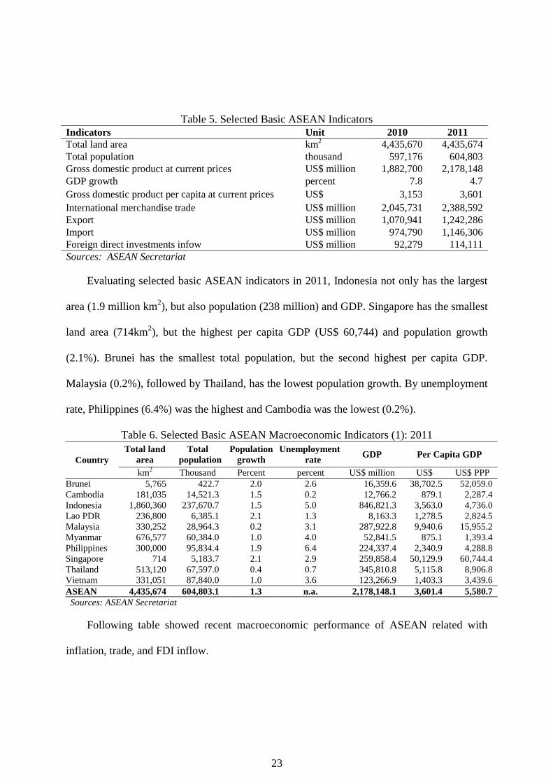
Evaluating selected basic ASEAN indicators in 2011, Indonesia not only has the largest

area (1.9 million km2), but also population (238 million) and GDP. Singapore has the smallest

land area (714km2), but the highest per capita GDP (US$ 60,744) and population growth

(2.1%). Brunei has the smallest total population, but the second highest per capita GDP.

Malaysia (0.2%), followed by Thailand, has the lowest population growth. By unemployment

rate, Philippines (6.4%) was the highest and Cambodia was the lowest (0.2%).

Table 6. Selected Basic ASEAN Macroeconomic Indicators (1): 2011

Country

Total land

area

Total

population

Population

growth

Unemployment

rate GDP Per Capita GDP

km2 Thousand Percent percent US$ million US$ US$ PPP

Brunei 5,765 422.7 2.0 2.6 16,359.6 38,702.5 52,059.0

Cambodia 181,035 14,521.3 1.5 0.2 12,766.2 879.1 2,287.4

Indonesia 1,860,360 237,670.7 1.5 5.0 846,821.3 3,563.0 4,736.0

Lao PDR 236,800 6,385.1 2.1 1.3 8,163.3 1,278.5 2,824.5

Malaysia 330,252 28,964.3 0.2 3.1 287,922.8 9,940.6 15,955.2

Myanmar 676,577 60,384.0 1.0 4.0 52,841.5 875.1 1,393.4

Philippines 300,000 95,834.4 1.9 6.4 224,337.4 2,340.9 4,288.8

Singapore 714 5,183.7 2.1 2.9 259,858.4 50,129.9 60,744.4

Thailand 513,120 67,597.0 0.4 0.7 345,810.8 5,115.8 8,906.8

Vietnam 331,051 87,840.0 1.0 3.6 123,266.9 1,403.3 3,439.6

ASEAN 4,435,674 604,803.1 1.3 n.a. 2,178,148.1 3,601.4 5,580.7


Following table showed recent macroeconomic performance of ASEAN related with

inflation, trade, and FDI inflow.

24

Table 7. Selected Basic ASEAN Macroeconomic Indicators (2): 2011

Country Inflation

rate

Exchange rate

at end of period1 Exports Imports

Total

Trade

Exp/

GDP

Imp/

GDP

Trade/

GDP

Percent

National

Curr./US$ Currency US$ mill US$ mill US$ mill % % %

Brunei 2.0 1.26 Dollar (B $) 12,362.3 2,460.0 14,822.3 75.6 15.0 90.6

Cambodia 5.5 4,079 Riel 6,710.6 6,133.6 12,844.1 52.6 48.0 100.6

Indonesia 3.8 8,775 Rupiah (Rp) 203,496.7 177,435.6 380,932.3 24.0 21.0 45.0

Lao PDR 7.6 8,011 Kip 1,746.5 2,209.4 3,955.9 21.4 27.1 48.5

Malaysia 3.2 3.06 Ringgit (RM) 228,179.1 187,542.8 415,721.9 79.3 65.1 144.4

Myanmar 5.0 766.59 Kyat 8,119.2 6,805.9 14,925.1 15.4 12.9 28.2

Philippines 4.6 43.39 Peso (PhP) 48,042.2 63,709.4 111,751.6 21.4 28.4 49.8

Singapore 5.2 1.26 Dollar (S $) 409,443.5 365,709.1 775,152.6 157.6 140.7 298.3

Thailand 3.8 30.49 Baht 228,820.7 230,083.6 458,904.4 66.2 66.5 132.7

Vietnam 18.6 20,510 Dong 95,365.6 104,216.5 199,582.1 77.4 84.5 161.9

ASEAN n.a. n.a. n.a. 1,242,286.4 1,146,305.9 2,388,592.3 57.0 52.6 109.7

Note: For ASEAN figure, exports, imports, and total trade are summation of all members; while others are average value


Vietnam has the highest inflation rate (18.6%) in ASEAN, and also, the least valued

currency. Singapore has the strongest currency, the highest FDI inflow, and the highest degree

of openness compared with other countries. Brunei has the lowest inflation rate (2%), and in

terms of trade, Myanmar has the lowest degree of openness (28.2%).

2.3.2 Timetable

Indonesia, Malaysia, the Philippines, Singapore, and Thailand established ASEAN on 8

August 1967. Later, Brunei Darussalam joined on 8 January 1984, Vietnam on 28 July 1995,

Laos and Myanmar on 23 July 1997, and Cambodia on 30 April 1999 (www.aseansec.org).

The main goals of ASEAN were long-lasting peace and common security in Southeast Asia.

The ASEAN Declaration states that the aims and purposes of the Association

(www.aseansec.org) are:

1. To accelerate economic growth, social progress, and cultural development in the region.

http://www.aseansec.org/

25

2. To promote regional peace and stability through abiding respect for justice and the rule of

law in the relationship among countries in the region and adherence to the principles of the

United Nations Charter.

Hill and Menon (2010) defined ASEAN by four broad characteristics:

1. It is a region of great diversity in economic, political, cultural, and linguistic diversity,

related with colonial experiences;

2. Most countries achieved rapid economic development over the past 25 years, longer in

some cases;

3. Diplomacy and cooperation have been characterized by caution, pragmatism, and

consensus-based decision-making;

4. ASEAN has never been, and probably will never be, an EU-type organization, nor a

NAFTA-type economic bloc.

The economic collaboration among ASEAN member states began in the 1970s. The

signing of the Preferential Trading Agreement (PTA) in 1977 was the first step in economic

integration. The impact, however, was not significant, since the countries were not ready to

open national borders and the development gap among countries was considerable.

According to Vanderon (2005), the key development phase was concluded in January

1992, when ASEAN leaders decided to take their trade liberalization efforts to a higher level.

To do so, they established the AFTA to promote the region‘s competitive advantage as a

single production unit and to eliminate tariff and non-tariff barriers among member countries.

Moreover, in 1995, they also concluded the supplementary ASEAN Framework Agreement

26

on Services (AFAS), and in 1998, ASEAN ministers established the ASEAN Investment Area

(AIA). Other major integration-related economic activities of ASEAN include the following

(Vanderon, 2005):

The Roadmap for Financial and Monetary Integration of ASEAN, addressing four areas,

namely, capital market development, capital account liberalization, liberalization of

financial services, and currency cooperation;

A trans-ASEAN transportation network consisting of major interstate highway and

railway networks, including the Singapore to Kunming Rail-Link; principal ports and sea

lanes for maritime traffic; inland waterway transport; and major civil aviation links

The Roadmap for Integration of the Air Travel Sector;

Interoperability and interconnectivity of national telecommunications equipment and

services, including the ASEAN Telecommunications Regulators Council-Mutual

Recognition Arrangement (ATRC-MRA) on Conformity Assessment for

Telecommunications Equipment;

Trans-ASEAN energy networks, specifically the ASEAN Power Grid and the Trans-

ASEAN Gas Pipeline Projects;

The Initiative for ASEAN Integration (IAI), focusing on infrastructure, human resource

development, information and communications technology, and regional economic

integration, primarily in the CLMV countries;

The Visit ASEAN Campaign and the private sector-led ASEAN Hip-Hop Pass to promote

intra-ASEAN tourism; and

Agreement on the ASEAN Food Security Reserve.

27

The ASEAN Vision 2020 was adopted in Kuala Lumpur by ASEAN leaders on the 30th

Anniversary of ASEAN. This set forth a shared vision of ASEAN as ―a concert of Southeast

Asian nations, outward looking, living in peace, stability and prosperity, bonded together in

partnership in dynamic development and in a community of caring societies‖

(www.aseansec.org). ASEAN Vision 2020 defines the AEC end goal as economic integration,

establishing ASEAN as a single market and production base, turning characteristic diversity

into complementary business opportunities, and making ASEAN more dynamic, a stronger

part of the global supply chain. In 2003, ASEAN leaders resolved that an ASEAN community

should be established with three pillars: the ASEAN Security Community, the AEC, and the

ASEAN Socio-Cultural Community.

Table 8. ASEAN Timetable 1961 Maphilindo and ASA

1967 Establishment

1971 Reorganizing in Bali

1976 ASEAN Concord I

1977 ASEAN swap arrangement

1978 Trade Preference Arrangement

1979 Security Reserve Agreement

1980 Industrial Project

1981 Finance Corporation

1984 Brunei joins

1992 AFTA and CEPT

1995 Vietnam joins

1997 Laos and Myanmar join

1999 Cambodia joins

2003 Concord II+3, AEC by 2020

2003 AFTA&CEPT start

2005 ASEAN Charter

2007 FTA with China, Japan, South Korea, Australia, India, New Zealand

2007 Accelerating AEC by 2015 Source : Adapted mainly from ASEAN Secretariat.

AEC goals fall in four market areas (four freedoms): goods, services, investment and

capital, and (skilled) labor. Thus, targets were based on AEM modalities. Current AEC

http://www.aseansec.org/64.htm

28

specifications refer mostly to border measures3 concerning regional trade and factor mobility,

factor movements (at the border), beyond- (or inside-) the-border measures4

, regional

standardization and harmonization of technical regulations, standards and conformance

assessment requirements of competition policies, business taxes and regulations of financial

and capital regimes and standards, and use of a common currency5 (www.aseansec.org).

According to Wattanapruttipaisan (2006), in a bid to achieve the AEC‘s targets, ASEAN

will face some risks and challenges. First, Intra-regional:

A large development divide and slow income convergence in ASEAN over time

Persistence of big gaps in institutional development and implementation capacity within

ASEAN

Crisscrossing FTAs by ASEAN and ASEAN Member Countries

Low levels of IP creativity and innovation

Persistent, heavy dependence on low-value-added external technologies, and FDI

Natural disasters and environmental degradation

Mass outbreaks of communicable diseases, and

Terrorism and crimes.

Their second set of challenges will be Extra-regional:

Interruptions in oil supply and persistence of high oil prices

Increasing market competition from China and India

3 removal of tariffs and a variety of non-tariff barriers (NTBs) on regional trade

4 no discrimination regarding regional sources of traded goods, services, and factor inputs inside member

countries‘ borders and across-the-border measures 5 a single (regional) market does not necessarily require or imply the use of a single currency or monetary union

29

Natural and financial resources and off-shore services

On-going advances in ―disruptive‖ technologies, and commercial breakthroughs in

consumer and producer goods

Ever-rising thresholds for performance and productivity from producers, service suppliers,

and workers

More sophisticated, exacting, and fickle consumer and market demands

Delayed negotiations and/or modest achievements under the Doha Development Agenda

Geo-political problems, including those in East Asia

Regional terrorism and crime.

The AEC‘s goal is to create a stable, prosperous, and highly competitive ASEAN

economic region, where there is a free flow of goods, services, and investment capital,

resulting in equitable economic development and reduced poverty and socio-economic

disparities by 2020. The AEC establishes ASEAN as a single market and production base,

using the region‘s characteristic diversity to develop opportunities for business cooperation,

making ASEAN a more dynamic and stronger contributor to the global supply chain.

ASEAN‘s strategy consists of the integration of ASEAN and enhancements to ASEAN‘s

economic competitiveness. To move toward implementation of an ASEAN Economic

Community, ASEAN‘s members agreed on the following (www.aseansec.org):

Instituting new mechanisms and measures to strengthen the implementation of its existing

economic initiatives, including the AFTA, the ASEAN Framework Agreement on

Services (AFAS), and the ASEAN Investment Area (AIA);

30

Accelerating regional integration in the following priority sectors by 2010: air travel,

agro-based products, automotives, e-commerce, electronics, fisheries, healthcare, rubber-

based products, textiles and apparels, tourism, and wood-based products.

Facilitating movement of business persons, skilled labor and talent; and

Strengthening the institutional mechanisms of ASEAN, including improvement of the

existing ASEAN Dispute Settlement Mechanism, ensuring expeditious and legally-

binding resolution of any economic disputes.

At the 13th ASEAN Summit in Singapore, ASEAN leaders committed to the ASEAN

Economic Blueprint as a coherent master plan guiding the establishment of the ASEAN

Economic Community by 2015. In Brunei, at the 22nd ASEAN Summit, ASEAN leaders

emphasized the importance of human resources as a central element of a post-2015 vision and

agreed to intensify work toward an ASEAN Community (www.asean.org).

31

Chapter 3 Literature Review

3.1 Economic Integration

Regional integration has become a global trend, resulting in greater reliance on market

forces, increased openness, and deeper integration into the world economy. These same forces

are expected to generate faster economic growth, especially for poorer countries, and lead to

the convergence of neighboring countries‘ income. Integration among neighboring countries

has been characterized by loose and speculative discourse. According to Agenor (2003), the

primary reason for the increase in integration around world is the concurrent increase in

globalization spurred by investors seeking the highest return.

Until recently, economic integration has generated important debate among economists.

Both theoretical and empirical works have been motivated by regional development issues

within the EU, ASEAN, NAFTA, and others. Jovanovic (2006) defines economic integration

as a process, the means by which a group of countries attempts to increase their communal

welfare, creating strong partnerships to more easily achieve common goals. The integration

process encourages communication and concern among member states, more than nations

outside any proposed union. De Rosa (1998) defines economic integration broadly as the

equalization of relative prices for traded goods among countries.

Jovanovic (2006) isolates international economic integration between at least two

countries into seven stages:

32

1. PTA

This trading bloc gives preferential access to certain products from participating countries,

by reducing tariffs, not removing them fully. A PTA can be established through a trade

pact, with the goal of a free-trade area.

2. Partial Customs Union

This type of trading bloc retains tariffs among members, introduces common external

tariff policy, and changes import quotas. These steps are meant to increase economic

efficiency and establish closer political and cultural ties among member countries.

3. Free-Trade Area

A free-trade agreement eliminates tariffs, quantitative restrictions, and purchasing

preferences on most goods and services traded among trade bloc members. If economic

structures are complementary, countries are most likely to choose this type of economic

integration, with a customs union the second choice.

4. Customs Union

Member countries remove all tariffs and quantitative restrictions among members and

introduce common external tariff with non-members, and also agree to common external

trade policy.

5. Common Market

This type of trade bloc is based on free mobility of factor production among members, and

common regulations and restrictions on non-members, to encourage easy movement of

factor production. Physical, technical, and fiscal barriers among member states are

removed to the maximum extent possible.

33

6. Economic Union

Trade bloc encompasses a common market, a customs union, and a monetary union. It is

established through a currency-related trade pact synchronizing monetary, fiscal,

industrial, transport, and other economic policies.

7. Total Economic Union

In the final stage of economic integration, a supranatural government is created, with

common economic policy and considerable economic authority. Integrated units have

negligible, or no, control over economic policy, including the harmonization of the

monetary union and fiscal policy.

Baldwin and Forslid (2000) proposed two major mechanisms by which economic

integration dynamically influences the evolution of an economy:

A scale-effect channel resulting from positive spill-over and the growth rate of the

integrated economic area.

A factor-reallocation channel resulting from the share of resources allocated to dynamic

economic sectors, changing the growth rate.

Integration can also be evaluated through the agglomeration effect, first developed by

Lösch in 1944 (in Neibuhr and Stiller, 2002). In his work, he develops a consistent, albeit

rather unknown, model dealing with spatial effects of economic integration. According to his

model, consumers and production factors are assumed immobile and equally distributed in

space. Lösch considers economies of scale and imperfect competition, by which firms

relocate where spatially dispersed demand can be best, served, while maximizing potential

34

profit. Therefore, transportation costs for goods should be proportional to the distance

between consumers and producers.

Hoover (in Niebuhr and Stiller 2002) discusses the significance of borders in traditional

location theory. He shows that tariffs and other restraints on international trade raise

transportation costs, distort market areas and supply networks, and increase the costs of

producers located near borders. Therefore, producers will avoid territory near a trade barrier

that might restrict their market or supply area, preferring to choose an area more central to

domestic markets. This border effect theorizes that firms orientate towards the interior of an

area enclosed by borders, since demand-and-supply relationships are denser in the

geographical center of a country than in its periphery.

Hoover suggests that the aperture of a border for trade may dramatically change the

economic situation in border regions. Border regions become more attractive to investors

through the reduction of international trade barriers and low-cost access to foreign markets.

Such conditions will spur relocation of firms to areas closer to a national border. When the

national market is not large, new products can be supplied profitably by a firm located near

the center of the common market. Therefore, through the process of integration, regions at the

boundaries of domestic and the foreign markets attract production.

Viner (1950) shows that integration will reduce trade barriers and increase international

trade, which affects international specialization in production. Intra-country reallocation of

production will drive economic adjustment, since production factors are assumed to be mobile

within countries and among sectors, though immobile internationally. Thus, countries develop

fixed-factor endowments, and trade serves as a substitute for factor mobility. Transportation

35

costs, whether on a national or international level, are treated as a single geographic location.

The assumption that spatial distance is irrelevant for the intensity of trade relations strongly

contrasts empirical estimations of gravity models proving that distance is a very important

determinant of international bilateral trade volume. As long as trade models neglect

international factor mobility, the value of this inherent element of integration is lost.

Krugman (1991) proposes new economic geography to address the distribution of

economic activities across space, explaining regional disparities by entirely endogenous

location decisions. Krugman‘s model is called the ―core-periphery model.‖ This model uses a

combination of elements from both traditional regional science and new trade theory.

Krugman‘s models were typified by explicit spatial structure, interregional trade costs,

economies of scale in production, and monopolistic competition. Since spatial equilibrium

results from the location decisions of firms, workers, and consumers, the balanced distribution

of workers and firms across space depends on the relative strength of centripetal forces

(promoting the geographic concentration of economic activities) and centrifugal forces

(promoting the geographic dispersion of economic activities). If centripetal forces dominate,

workers and firms will be unequally distributed. Therefore, he suggests that there are

agglomerations with a high density of economic activities, as well as regions with only a few

firms, or no industry at all.

Niebuhr and Stiller (2001), studying the spatial impact of integration, showed two highly

relevant economic geography hypotheses:

Eliminating international trade costs and liberalizing the movement of cross-border labor

will affect the balance of centripetal and centrifugal forces on the international level. This

36

integration will change the distribution of population, production factors, and firms

among countries. Therefore, the spatial impact of integration may increase labor

migration among countries. This labor migration will alter both national factor

endowments and the international location of industrial activities.

Eliminating international trade costs will change the balance of centripetal and centrifugal

forces on a national level, since foreign markets become more important for buyers and

suppliers. Thus, integration will change the distribution of population, production factors,

and firms within countries. This implies that opening goods markets might affect the

economic geography within a country because the location of economic activities within

a closed economy is strongly inward-oriented, so such changes move toward an outward

orientation in an open economy. The domestic market becomes less important and less

attractive, which may cause reallocation of economic resources within a country away

from previous centers to new locations.

Niebuhr and Stiller theorize that integration has a positive impact on foreign demand,

potential markets, and cross-border backward and forward linkages. But these developments

favoring economic activity in border regions are countered by forces intending to preserve

pre-integration geography of economic activities. Hence, economic theory only allows very

vague conclusions about the spatial effects of integration. The relative weight of these

counteracting forces is ambiguous from the theoretical perspective. Results depend on

specific circumstances, under which border regions might see benefits, losses, or no effect

from integration.

37

Baldwin and Wyplosz (2012) define integration effects of growth into medium- and long-

term. Medium-term effects, they say, are sequential economic integrationimproving efficiency,

higher GDP per worker, and higher investment per worker. From this point, the capital-per-

labor ratio shows higher value and faster growth of output per worker. Long-term effects are

faster knowledge creation and absorption. This arises from increased investment in

knowledge, leading to a permanent increase in growth.

In the case of financial integration, Agenor (2001) defined some benefits : consumption

smoothing, whereby a country can borrow money in recession and lend money when

booming; domestic investment and growth, whereby openness provides access for domestic

investment, contributing to growth; enhanced macroeconomic discipline, whereby free flow

of capital will punish bad policy and reward good policy; and increased banking system

efficiency and financial stability, since foreign banks will improve the overall quality and

resources of the financial system).

On the other hand, Agenor writes that costs may also arise from: concentration of capital

flows and lack of access, domestic misallocation of capital flows, loss of macroeconomic

stability, pro-cyclicality of short-term flows, herding, corruption and volatility of capital flows,

and risks of entry by foreign banks.

3.2 Economic Crisis

According to Stiglitz (2010), integration of global markets was supposed to lead to

greater financial stability, as risks were spread around the world; however, recent financial

crises have thrown doubt on this conclusion; in the absence of appropriate government

intervention, private transactions for profit may lead to systemic risk. The crisis suffered by

38

the Eurozone repeated the story of crises experienced by Latin America and Asia; however,

the Eurozone was, of the three, by far the most developed area, well-known for its global

economic and political power. The crisis happens in the area which all member countries had

surrendered their currency policy to ECB avoiding them to adjust the nominal currency.

Palley (2011) followed a Minskian framework, hypothesizing that the Eurozone crisis

resulted from instability of capitalist economic processes. Thus, Minsky (1977) emphasized

the importance of adequate governmental constraint on private institutions to stabilize the

economy.

Radelet and Sachs (2000) defined the five main types of financial crisis as:

1. Macroeconomic Policy-Induced Crisis, a balance-of-payment crisis involving currency

depreciation, loss of foreign exchange reserve, or collapse of a pegged exchange rate.

2. Financial Panic, an adverse equilibrium outcome in which short-term creditors suddenly

withdraw their loans from a solvent borrower.

3. Bubble Collapse, occuring when speculators purchase financial assets at a price above their

fundamental value in order to realize capital gain.

4. Moral-Hazard Crisis, wherein banks borrow funds on the basis of implicit or explicit public

guarantees of bank liabilities.

5. Disorder Workout, in which an illiquid or insolvent borrower provokes a creditor grab race

and forced liquidation, even though the borrower is worth more as an ongoing enterprise.

Stiglitz (2000) theorized that capital market liberalization was responsible for the

Eurozone crisis, based on standard efficiency arguments, employing a conventional

neoclassical model and ignoring differences between financial and capital markets and

39

markets for ordinary goods and services. He ignored distributional consequences, presumably

believing that if gains are large enough, benefits will trickle down to the poor. He argues that

international competition for funds requires countries to create an attractive environment to

business. He also proposes that open capital markets help stabilizes the economy through

diversification and funding for needed investment projects. Stiglitz‘s empirical study stressed

that there exists no strong relation between growth and liberalization stability, that capital

market liberalization mainly produces instability, not growth, since financial and capital

markets are different from markets for ordinary goods and services. Furthermore, he writes,

financial openness only facilitates the flow of capital, rather than providing another channel

for adverse effects.

The cause of the Eurozone crisis might also be explained by Minsky‘s financial

instability hypothesis, which states that inadequate controls by the government on private

industry led to natural capital instability (Minsky, 1977). Tse (2001) depicted big government

and big banks as the two most important economic institutions, applying Minsky‘s analysis to

the current situation in Europe. Palley (2011) proposed that capitalism demonstrates an

inevitable tendency toward instability. This view might be expressed as: “success breeds

excess breeds failure (Minsky, 1977).‖ Evolutionary factors are present because an economy

evolves through stages that breed successive stages. Instability is present because the system

periodically ends in failure and collapse. This hypothesis defined two cyclical processes:

1. Basic cycle

The basic cycle considered consumer psychology about market conditions, beginning

with progressive optimism, when optimistic valuations of assets and investment revenue

40

streams are combined with an increased willingness to take on risk. The situation was critical

that urges weakening market discipline, and emphasizing the emergence of gradually more

fragile corporate balance sheets. It was marked by either reduced liquidity or higher debt-

equity ratio. The chronicle stages were as follows:

a. Hedge Finance, or financial tranquility. At this stage, all agents can fulfill their

contractual payment obligations by their cash flows. This condition tends to be associated

with higher equity financing in the liability structure.

b. Speculative Finance, or financial fragility. At this stage, agents can fulfill their payment

commitments through income accounts on their liabilities. In this stage, they unable to

repay loan principle out of cash flows.

c. Ponzi Finance, or financial bust. The agents in this stage recognize that their cash flows

from operations are not sufficient to fulfill either the repayment of principle or the

interest due on outstanding debts by their cash flows from operation. The only ways to

achieve liquidity are selling assets or borrowing.

2. Super cycle

The super cycle is a process of transforming business institutions, business practices,

conventions, and the structures governing the market in a fashion that eventually gives rise to

a major financial crisis. Palley‘s major concern was that the governmental structures were

required to ensure the stability of capitalist economies, both public and private, with the goal

of constraining outcomes, even when instability might not be observed.

Generally, the process of erosion and transformation was characterized by a super cycle

taking several cycles simultaneous to the basic cycle. By this definition, financial busts only

41

happen once a generation, when Minsky‘s super cycles erode the economy‘s regulating

institutions. At this stage, systemic stability is threatened by expanded risk taking, systemic

exuberance, and the systemic vulnerability that occurs with excessive risk. This cycle

demonstrates twin developments which are regulatory relaxation and increased risk-taking.

3.2.1 Asian Crisis

As demonstrated by the Asian financial crisis of 1997 year, Kaminsky and Reinhart

(1998) pointed out that financial crises occur as an economy enters a recession, following a

prolonged boom in economic activity fueled by credit creation and surges in capital inflow.

Miskhin (1999) emphasized the Asian financial crisis was not only disastrous regionally, but

also placed the global financial system under tremendous stress.

Wade (1998) demancated four steps leading to the Asian crisis:

1. The exchange collapse

2. An upsurge of bank failures and company bankruptcies resulting from the costs of

unhedged foreign debt

3. A domestic recession resulting from falls in consumption and investment, as well as

rising unemployment; and

4. Political reaction from the economic slump.

Wade‘s detailed chronology of the Asian crisis explores the underlying reasons for the

economic downturn:

42

1. A capital push in 1985, when Japanese companies sought a new, cheaper manufacturing

base in a US-dollar zone. Southeast Asia was the obvious choice—close to Japan,

currency pegged to the US dollar, and cheap, well-educated workers.

2. Very cheap credit in Japan and strong Japanese government support helped to stimulate a

Japanese investment and export boom. Rising exports sustained more borrowing, more

equity issues, and more FDI.

3. Additionally, capital liberalization occurred when Asian countries operated a fixed

exchange rate pegged to the US dollar. Concurrently, radical financial deregulation in the

1990s removed restrictions on the inflow and outflow of mobile capital.

4. The deregulation happened with little attention to the new kinds of regulations that would

be required and with only a thin base of financial skills.

5. The deregulated financial systems enabled inexperienced private domestic banks and

firms to take out large, dollar-denominated loans from foreign lenders and on-lend with

generous spreads, especially in Thailand.

6. Before the huge inflow of capital, Asian households saved money. Gross Domestic

Savings are typically one-third of GDP. East and Southeast Asia are low-income regions,

however, where capital is more abundant than in the higher-income regions of North

America and Europe.

7. A very high rate of domestic savings intermediated from households to firms via banks,

creating a deep structure of domestic debt.

43

8. The crisis started with inflationary pressure; the inflow of financial capital, combined with

a fixed exchange rate, forced an increase in domestic money supply, fuelling inflation at

around 6%.

9. Then came major shifts in the exchange rate when the US dollar appreciated against other

currencies. The appreciation of the dollar, coupled with domestic inflation at rates higher

than trading partners, created a squeeze on exports and devaluation of imports.

10. Responding to high savings, domestic inflation higher than trading partners, and reduced

prospects for export-oriented manufacturing, investors in Southeast Asia invested in real

estate.

11. Property speculation flourished continually as foreign currency continued to pour in and

domestic money supply continued to expand.

12. As consumers expected continued inflation, property investments appeared to be the best

hedge.

13. As a result, Thailand‘s private sector property bubble burst in 1995, and the stock market

crashed in 1996.

14. In May 1997, Japanese officials hinted that they might raise interest rates. The threat of a

rise in Japanese interest rates, plus concerns about Thailand‘s currency, raised fears

among commercial bankers, investment bankers, and others.

15. The contagion effect of the crisis finally spread across East and Southeast Asia.

Radelet and Sachs (2000) showed the reasons for the severe crisis in Asia:

Large-scale, unanticipated, involved, unguaranteed lending to debtors, leading to lack of

credit for viable enterprises

44

Positive market reaction to initiate that bring creditors and debtors together for orderly

workouts

Triggering events leading to the sudden withdrawal of investor funds.

According to Radelet and Sachs (2000), the Asian crisis would not have been so severe

if certain conditions had been met:

If Japan had addressed its banking problem earlier

If the Japanese government had pledged 10 billion rather 4 billion

If the US Congress had been less isolationist

If developing countries liberalized their financial systems more slowly

If developing country political leaders had been prepared to check wild real estate

investment and speculation in junk bonds

If there had been sand in the wheels of the international financial system, such as a tax on

international currency transactions, and

If the IMF stuck to its mandate of helping countries to cope with temporary foreign

exchange shortages.

Radelet and Sachs (2000) also concluded that the Asian crisis was unpredictable. Since

capital inflows remained strong, risk premiums were attached to loans to emerging market

economies. The assessments from credit-rating agencies were good, as were and investment

forecasts. These conditions were supported a government debt in surplus and very high

domestic saving and investment rates. The strong world market did not portend a crisis.

However, the crisis emerged after risk expanded through growth of current account deficits,

45

an overvalued exchange rate, slowing export growth, and increasingly fragile financial

institutions, deteriorating throughout the 1990s.

3.2.2 The Eurozone Crisis

The current Eurozone crisis, which began in the USA, now spread through the

Eurozone—in fact, the entire world. The sovereign debt crisis in the euro zone is a symptom

of failures and deficiencies in fiscal policy coordination (Schuknecht, et. al, 2011). The

inception of EMU in the early 1990s followed a period characterized by big public

expenditure, chronic budget deficits, and rapidly rising public debt ratios in many of the

future EU countries.

The crisis suffered by the Eurozone resembled similar crises experienced by Latin

America and Asia; however, this crisis was in one of the most developed areas in the world.

The Eurozone maintains a very high level of global economic and political power, due to its

relative stability. Until the crisis erupted in 2007, the euro gained a reputation as a stable

anchor and strong currency. However, according to Obstfeld and Rogoff (2009), three trends

of unsustainability appeared increasingly:

1. Real estate values were rising at a high rate in many countries, including the USA, the

world‘s largest economy.

2. A number of countries were simultaneously running high, and rising, current account

deficits.

3. Leverage had built up to extraordinary levels in many sectors across the globe.

46

Debate among economists arises around the responsible factors for the crisis in Europe.

Some economists argue that external imbalances, or financial regulatory failures and policy

errors, were responsible, but others believe there is a cross-relation between them. Among

researchers, Obstfeld and Rogoff (2009) believed that global imbalances and the financial

crisis are intimately connected. The relationship between Germany and peripheral nations

resembled the trade imbalance between the US and China.

Perez-Caldentey and Vernengo (2012) explained that the original source of external

crisis was a domestic debt crisis, combined with self-fulfilling expectations and financial

sector imbalances. They showed that the stylized crisis depicted in the Keynesian framework

indicated an inability to keep labor cost growth in the peripheral countries of Europe. This led

to a loss of competitiveness and increasing external problems when combined with a financial

crisis, resulted in a collapse of output and a fiscal crisis. The problem of competitiveness

festered, because there was no depreciation mechanism for the nominal exchange rate, and

there was an absence of supra-national fiscal authority to transfer resources. The only possible

solution for external imbalances was fiscal contraction.

Bellofiore, Garibaldo, and Halevi (2010) charged that China and Germany conducted

neo-mercantilist behavior, a biased policy to maintain a foreign trade surplus. In the Eurozone,

German behavior during the crisis has been consistent with its traditional economic stance—

non-cooperative at the global and European levels, relying on domestic price stability and

export-led growth. Devaluation of the Euro improved German export competitiveness.

Unfortunately, Germany profited from its neighbors‘ sacrifice. Peripheries couldn‘t recover

47

due to tightening fiscal policy encouraging price stability, and a lack of full control of

monetary policy.

Germany‘s behavior before and during the crisis has also been consistent with neo-

mercantilism behavior as described by Cesaratto and Stirati (2011):

Taking advantage of a fixed exchange rate by pursuing a domestic inflation rate lower

than competitors to foster exports;

Relying on other countries‘ stimuli to aggregate demand, and taking advantage of their

ensuing inflationary bias;

Compensating with conservative domestic fiscal (and monetary) policy and possible

labor market overheating, maintaining the external competitive hedge; and

Replying to foreign criticism with moralistic tones, blaming their lack of discipline and

proposing itself as a model.

Based on this study, monetary mercantilism is defined as price stability guaranteed by

an independent central bank in the context of fixed exchange rates., and thus, the opportunity

to gain competitiveness by keeping domestic inflation lower than competitors in the context

of a fixed exchange rate regime. Hidden behind the centrality of price stability, the trade

surplus became the central target of German policy.

Later, Germany obtained the same combination of lower domestic inflation and fixed

exchange rates through the adoption of the EMU. Fiscal policy sustained the mercantilist

strategy both in macroeconomic terms, by repeatedly posting budget surpluses to help tamp

down domestic demand, and in microeconomic terms, by fiscal support to the export sector.

48

Whyte (2010) highlighted that the combination of trade surplus stemming from export-

led growth, wage moderation, and domestic demand compression became the benchmark of

Germany‘s long-term advantage over competitors. Therefore, Germany can be considered a

mercantilist country.

Schuknecht (2011) showed that policy failures and deficiencies—particularly fiscal

policy coordination—were the primary main causes of the recent crisis. The first nine years of

the euro were not used effectively to improve public finances, and the Stability and Growth

Pact (SGP) was neglected.

According to Vines (2011), inappropriate policy-making system was adopted has a

direct consequence of the crisis. Launching the euro coin and paper currency for new

members was based on the nation in question having fulfilled convergence criteria, including

benchmarks for inflation, interest rates, exchange rates, deficits, and debt.

After the euro was introduced, interest and inflation rates converged at lower levels,

which led to rapid mobilization of financial flows across borders, accelerating inflation rate

and interest rate convergence. The ECB successfully accomplished its monetary goals. Low

inflation and interest rates fueled a credit boom from 2003 to 2007, thereby increasing

business-cycle fragility.

Credibility of ECB on inflation targeting accompanied by economic growth, induced

optimism in financial market and the euro seen as a stable common currency. Investment

soared as currency risk dramatically diminished, and competition boosted financial innovation,

since firms and financial institutions could borrow easily from abroad. Investment growth in

Peripheries was concentrated mainly in the housing sector, encouraging rapid growth of

49

construction and financial services, and a property boom. Credit growth translated into a

buildup of debt. Faster growth experienced by peripheries increased consumption and demand

for imports, and resulted in larger current account deficits. High economic growth meant rapid

expansion of credit and property valuation. Without enough control of the private sector, as

predicted by Minsky‘s hypothesis (Palley, 2011), mortgages, as well as banks relying heavily

on wholesale external borrowing, created a state of financial fragility. Consequently, property

prices crashed in 2009. Governments were not able to overcome large losses without outside

support.

In response to the global financial crisis of mid-2007, the European Commission

launched European Economic Recovery Reform (EERP). This plan coordinated short-term

budgetary stimulus for fiscal stabilization, in order to strengthen demand by 1.5% of GDP.

The reform also included capital injections for weak financial institutions. Unfortunately,

given current fiscal deficits, debt dynamics, and additional contingent and implicit liabilities,

major fiscal adjustments will be needed in almost all Eurozone countries over a long period of

time to ensure fiscal sustainability (Schuknecht, et. al, 2011).

3.3 Convergence

The term ―convergence,‖ according to many authors, is not without certain ambiguity.

Broadly, convergence can be defined two ways:

First, the process in which less-developed countries can catch up to developed countries

in terms of economic productivity and growth

Second, the equality of long-term forecasts at a fixed time (Bernard and Durlauf, 1996).

50

According to Zdaarek and Sindel (2009), convergence is a process approaching a

certain level or decreasing the difference between two values over time (the difference

between the two variables reduces over time toward a zero value).

In this research we focus mainly on the terms ―nominal‖ and ―real‖ convergence.

3.3.1 Real Convergence

The neoclassical growth theory is the foundation of the real convergence concept,

assuming convergence toward a steady status (identical for all economies), influenced by a

variety of characteristics and parameters of the relevant economies (savings, population

growth, degree of depreciation of capital assets, and so on). Basically, real convergence could

be defined as advancement of one country‘s economic standard towards the level of another

developed country or a group of countries (within an integrated group). This is commonly

measured by GDP per capita (Zdarek and Sindel, 2009).

Real convergence realizes different outcomes in long-run economic evolution and

convergence, such as per capita income, productivity, and the labor market (Marelli and

Signorelli, 2010). A long-run view of real convergence implies the narrowing of differences

in the structural condition of different countries (or regions), thus allowing the achievement of

similar performance of real variables or, more precisely, a catching-up in the transition period

of backward countries, in terms of standard of living, productivity, etc. A short-run view

stresses the business cycle features of economic growth of different countries.

Expanding on these definitions, two other broad analyses apply, which are

complementary, but not excludable:

51

1. , or sigma convergence, which measures the dispersion of per capita income or

productivity among different economies (regions or countries) over time. The

convergence, or variance convergence, implies that wealth differences are diminishing

among a set of countries or regions over time. These data are useful for observing periods

of convergence or divergence through time.

2. , or beta convergence, predicts the inverse relationship between the growth of per capita

income or productivity, and their initial levels. These dataexplicitly show the rate of

convergence across economies, implying that poor regions or countries grow faster than

richer ones. This concept is expanded to two further theories:

a. Absolute, or unconditional, convergence comes from standard neoclassical theory,

based on diminishing returns to capital properties. Free trade and perfect factor

mobility will guarantee the convergence result through the equalization of variables.

Under these circumstances, policies have no role in shaping long-term economic

growth. Empirical studies support the absolute convergence hypothesis only as a

special case, when the sample involves economies with a high degree of homogeneity.

b. Conditional convergence stems from ―new endogenous‖ growth theory, which

emphasizes the importance of human capital and innovation as the condition factors

for convergence. This theory relaxes the assumption of diminishing returns to

reproducible factors and states the possibility of constant, or even increasing, returns

to scale emanating from human and physical capital accumulation. With constant or

increasing returns to broad capital, the long-term rate of growth becomes endogenous,

52

depending on investment decisions, in turn influenced by policies and institutions.

Conditional convergence (conditional on the steady state) implies that there is a

negative partial correlation between the growth rate and the initial level of per capita

income. In this context, absolute convergence is not the rule. Economies converge to a

different steady state point, which depends mostly on human capital stock and capital

accumulation, among other structural factors. When the underlying differences in

technological progress and other factors are controlled in the convergence equation,

the initial value of per capita income turns out to be strong and significantly negative.

De la Fuente (2002) stated that the necessary conditions for convergence are: the

presence of decreasing return to scale of capital, and the presence of technological progress.

The fundamental factordetermining the level of convergence is investment in physical and

technological capital. Once a country suffers from a divergence in fundamental factors, it will

be difficult for this country to catch up to the growth process experienced by the higher-

income country. This view was supported by Ben-David (1998), who divides the world into

its wealthiest countries (the convergence requires catch-up by poorer countries) and its

poorest countries (the convergence requires downward movement by richer countries). This

division results from a positive relation between the savings rate and level of development.

The richer the country is, the higher the rate of savings, and the higher the level of

development will be.

53

3.3.2 Nominal Convergence

Nominal convergence, as defined by Zdarek and Sindel (2009), is a broader process as it

relates to the convergence of absolute values and growth rate in connection with Maastricht

Criteria (interest rate, inflation rate, deficit and public debt, and exchange rate criteria), and a

narrower process as it relates to the convergence of individual economies through their price

(and economic) levels. The relationship between real and nominal convergence, for example,

the relationship between the economic standard achieved (GDP per capita) and the price level,

is bilateral and mutually influential and determinative. Normally, countries at a lower

economic level have lower prices and wages. As standard of living increases, the price level

tends to rise (due to inflation and a rising exchange rate). This process gradually leads to the

elimination of cost-based competitiveness among local companies. If the economy is to retain

its dynamism, progress toward non-price competition is necessary.

According to the EU Commission, nominal convergence gradually leads to real

convergence, providing advantages like macroeconomic stability (price stability and fiscal

discipline), the removal of exchange risk, reduction of uncertainty concerning inflation and

interest rates, and stimulus of investment and international trade, all leading to stronger

economic growth. Because these benefits may be more important for deviating economies or

lagging countries, a real EU convergence is likely to occur in the long run.

3.4 Optimum Currency Area and Maastricht Criteria

Countries joining a common currency weigh the potential benefit of joining against the

inevitable cost (Mico, Stein and Ordonez, 2003). Benefits like a reduction in transaction cost

when trading goods and services between countries with different currencies will tend to

54

benefit countries heavily involved in international trade. On the other hand, costs may arrive

from the possibility of dampening business cycle fluctuation through independent, counter-

cyclic monetary policy.

In order to increase benefits and decrease costs, some economists suggest using an

optimum currency area (OCA) framework as the background theory. MT, with convergence

criteria, emphasizes the usefulness of the theory that a common currency will lead optimality

of the currency area, as stated by Mundel (1973).

Mundel (1961) defined OCA as: ―an economic unit composed of regions affected

symmetrically by disturbances and between which labor and other factors of production flow

freely.‖ Tavlas (1994) defines OCA as: ―a group of countries that maintain either a single

currency or though maintaining separate currencies, have rigidly fixed exchange rate among

themselves and full convertibility of the respective currencies into one another.‖ Mongelli

(2002) suggested that OCA was:

“The optimal geographic domain of a single currency, or of several currencies

whose exchange rates are irrevocably pegged and might be unified.”

Mongelli (2002), based on his survey study on OCA, demarcated four phases of OCA:

1. The Pioneering Phase (1960-1970) covered the foundation of theory, debated borders of a

currency area, and introduced OCA properties.

2. The Reconciliation Phase (1970-1980) examined OCA properties and additional Meta

OCA properties (business-cycle synchronization), and created a structural analysis of

costs and benefits.

55

3. The Reassessment Phase (1980-1990) introduced new OCA theory, reconsidering the

costs and benefits of monetary integration, and continuing debate on the size and timing

of currency areas.

4. The Empirical Phase (1990-present) reviewed all OCA properties in great detail to find

out how their interpretations have changed. In this phase, it was concluded that the

underpinnings of OCA theory were remarkably strong. Researchers also assessed why

specific groups of countries may form an optimum currency area.

Mongelli (2002) also differentiated the properties of OCA as:

1. Price and wage flexibility: When flexible, adjustment following a disturbance is less

likely to be associated with sustained unemployment in one country and/or inflation in

another.

2. The mobility of labor and other factor production: High factor market integration can

reduce the need to alter real factor prices and the nominal exchange rate in response to

disturbances.

3. Financial market integration: Such integration can reduce the need for exchange rate

adjustment.

4. The degree of economic openness: Higher degrees of openness translate to more changes

in international prices of tradable goods. This increases domestic cost of living and

reduces the potential for money and/or exchange rate illusion by wage earners.

5. Diversification in production and consumption: This will dilute the potential impact of a

shock on any particular sector.

56

6. Similarity in inflation rates: When inflation rates between countries are similar or lower

over time, terms of trade will also remain fairly stable. This will, in turn, foster more

equilibrated current account transactions and trade, and reduce the need for nominal

exchange rate adjustment.

7. Fiscal integration: Countries sharing a supra-national fiscal transfer system, which allows

them to redistribute funds to a member country affected by an adverse asymmetric shock,

also facilitate adjustments to such shocks and might require a lower nominal exchange

rate adjustment.

8. Political integration: Political will fosters compliance with joint commitments, sustains

co-operation on various economic policies, and encourages more institutional linkage.

Similarity of policy approaches is relevant in turning a group of countries into a successful

currency area.

9. Similarity in shocks: When shocks are more symmetrical, the benefit will be larger than

the cost of a common currency.

In Mundel (1961), policymakers balanced the savings in transaction cost from the

creation of a common currency against the consequences of diminished policy autonomy. The

loss of autonomy follows from the loss of exchange rate and of independent monetary policy

as instruments of adjustment. The costs are greater when macroeconomic shocks are more

asymmetric, when monetary policy is a more powerful instrument for offsetting them, and

when other adjustment mechanisms, like relative wages and labor mobility, are less effective.

The theoretical question—whether a single currency is beneficial for the participating

countries—dates back to Mundell (1961), who proposed that a single medium of exchange

57

should reduce transaction costs, and thereby facilitate international trade, but he also stated

that a single currency may be problematic in the case of coexisting asymmetric shock and

nominal rigidity. Therefore, he suggested perfect labor mobility as an indispensable condition

to lowering the stability losses associated with giving up monetary independence.

Mundell himself challenged his earlier proposal of a small currency union by

introducing the foreign exchange market and international risk sharing. In his later model

(Mundell, 1973), he suggested that the greater the number of countries involved, the better

they can mitigate shocks by reserve pooling and portfolio diversification. Warin, Wunnava,

and Janicki (2009) concluded that in the 1960s, Mundel argued that an economic area has to

be optimal before using a common currency or a fixed exchange-rate mechanism; however,

the causality was reversed in the 1970s—using a common currency or joining a fixed

exchange-rate mechanism may help an economic area become optimal. McKinnon (2004)

stated that a country could not participate in a common-currency regime if its own public

financial system was too weak, no sufficiently stable monetary standard exists in the rest of

the world.

Standard OCA theory explained that the net benefit of a monetary union is an increasing

function of the magnitude of trade, since trade creates opportunities for reaping efficiency

gains from currency unification (Kumakura, 2006). According to Eichengreen (1993), Europe

at the time was clearly not an OCA. Consequently, the Maastricht Treaty was implemented in

1993, in order to force convergence to an OCA prior to adoption of a common currency. Five

economic proxies were devised to ensure the convergence on the three public policy

dimensions: (1) monetary policy (in a closed- and open-economy perspective); (2) fiscal

58

policy; and (3) structural policy. The proxies were respectively: inflation, exchange rate,

national debt, public deficit, and long-term interest rates.

Schiavo (2006) summarized the effect of introducing a common currency for OCA,

identifying the following three characteristics:

1. It will sweep away one of the main determinants of market segmentation, increase asset

substitutability, and improve capital mobility.

2. It will encourage more tightly correlated cycles.

3. It provides better insurance for production risk and enhances specialization.

According to De Grauwe and Mongelli (2011), monetary integration has at least two

ways to foster endogeneity from market-based and institutional forces. Mongelli (2002)

summarized the benefits of a common currency as:

Microeconomic Efficiency: Liquidity serviced from common currency.

Macroeconomic Stability: Price stability and transparency.

Positive External Effect: From savings on transaction costs.

He determined the costs to be:

Microeconomic Inefficiency: Costs of switching to a new currency

Declining Macroeconomic Stability: Narrowing the menu of policy instruments

External Cost Effects: If a country suffers from a deteriorating position, it will impact on

other members

Preparing for deeper integration with a common currency, in 1991, heads of EU states

signed the MT. The Treaty was a strategy for moving towards a monetary union based on two

59

principles: the transition would be gradual, and entry into the union was conditioned upon

satisfying the following four convergence criteria:

1. Price Stability. The rate of inflation should not exceed the average rate of the three best

performers by more than 1½ percentage points.

2. Soundness of public finance. The deficit of the general government budget should not be

excessive.

3. Exchange rate stability. The exchange rate should have been kept within the normal band

of the Exchange Rate Mechanism (ERM) for at least two years, without a devaluation

against any other member‘s currency.

4. Durability. The long-term interest rate should not exceed the average rate of the three

countries with the best inflation performance by more than 2 percentage points.

This treaty stated that admission to the monetary union would not be automatic; therefore,

convergence criteria were needed (De Grauwe, 2009):

1. Inflation Convergence

This required criterion was based on the fear that a future monetary union would have

inflationary bias, if two countries were assumed to be identical except for their authorities‘

preferences, vis-à-vis inflation. Before the EU started, the candidate member countries

were asked to prove that their interest in having an inflation rate as low as those of the

low-inflation member countries. During this process, a temporary increase in

unemployment was inevitable (i.e., a movement along the short-term Philips curve). Self-

imposed suffering served as additional evidence that countries were committed to

lowering inflation. Once they achieved low inflation rates, they could be safely granted

60

membership. When a common central bank captures the monetary policy of each member,

it should reflect the average preference of the participating countries.

2. Interest Rate Convergence

The justification for this criterion is that excessively large differences in interest rates

could lead to large capital gains and losses. Suppose a country wanted to enter the

monetary union, but at the moment of entry, its interest rate was higher than that of the

monetary union zone. As a result, it would be quite attractive for bondholders to sell low-

yield monetary union bonds and buy high-yield candidate country bonds. Thus, economic

agents holding monetary union bonds would see capital losses, and economic agents

holding candidate members‘ bonds would see capital gains; either could create

disturbances in national capital markets.

3. Exchange Rate Convergence

The main motivation for this criterion is to prevent countries from manipulating their

exchange rates so as to force entry at a more favorable exchange rate (i.e., a depreciated

one, which could increase their competitive position).

4. Budgetary Convergence

High government debt creates an incentive to engineer surprise inflation. Suppose a

member country has long-term bonds with an interest rate fixed in a previous period,

based on prevailing inflation expectations. If the government were to create unexpectedly

higher inflation rates, the real value of these bonds would erode and the bondholders

would derive insufficient compensation, because the interest rate on their bonds does not

reflect this inflation upsurge. A monetary union between low- and high-debt countries

61

creates a problem for the low-debt country. In the union, the low-debt country will be

confronted with a partner who will have a tendency to push for more inflation. As long as

one country has a higher debt-to-GDP ratio, it will have an incentive to create surprise

inflation. As a result, the low-debt country stands to lose and force the high debt-to-GDP

ratio country to reduce it. Once this is achieved, the incentives to produce inflation

disappear, and the candidate country can be safely allowed into the union.

Perez-Caldentey and Vernengo (2012) highlighted the necessity of exchange rate

convergence criteria to avoid the manipulation of the exchange rate to achieve improved

competitiveness; inflation and budget convergence avoided of an inflationary bias. They

stated that fiscal criteria should require members have balanced budgets or be in a surplus

position in the medium-run, in order to offset deficits in times of economic downturn, and

interest rate criteria should limit opportunities for capital gains and losses prior to entry.

In managing monetary policy, The ECB set theoverriding objective of keeping inflation

low. It can certainly be concluded that the macroeconomic management conducted by ECB

has been successful from the initial stage of Euro, in the period before the crisis, and during

the early stages of the crisis. Inflation rates and interest rates were very low to help reverse the

downturn, and liquidity was injected.

The ECB‘s major problem was how to conduct monetary policies in a union where

asymmetric shocks occur. The ECB was responsible for maintaining price stability and

stabilizing the EU economy as a whole. In the extreme case of a pure asymmetric shock, the

ECB will never stabilize; it will experience complete economic paralysis. Thus, the

effectiveness of the ECB in stabilizing output in individual countries depends on whether

62

shocks are symmetric or asymmetric. However, in practice, shocks are always some mixture

of symmetric and asymmetric movements.

According to De Grauwe (2009), the ECB generally stabilizes too little from the point of

view of individual members. To reach price stability objectives, the ECB uses three types of

instruments: open market operations, implying buying and selling of securities with the aim of

increasing or reducing money market liquidity; standing facilities, aimed to provide and

absorb overnight liquidity from NCBs; and minimum reserve requirements, the imposition of

minimum reserves for banks.

The basic insight of this view is that a country that finds itself on an unsustainable path

of increasing government debt creates negative spillover effects for the rest of the monetary

union. A country that allows its debt to-GDP ratio to increase continuously will have increase

resources to the capital market of the union, thereby driving the union‘s interest rate upward.

The increase in the union‘s interest rate, in turn, increases the burden of the government debts

of the other countries. If the governments of these countries choose to stabilize their debt-to-

GDP ratios, they will be forced to follow more restrictive fiscal policies.

Thus, an unsustainable increase in the debt of one country forces other countries to

follow more deflationary policies. It will, therefore, be in the interest of these other countries

that a control mechanism should exist restricting the size of budget deficits in the member

countries. Based on the theory of optimum currency areas, this suggests that national fiscal

authorities should maintain a sufficient amount of flexibility and autonomy. The second found

its reflection in the MT and SGP. The conduct of fiscal policy in a monetary union has to be

disciplined by explicit rules on the size of the national budget deficits.

63

The OCA view is probably over-optimistic about national budgetary authorities using

budget deficits as instruments to absorb negative shocks. Although there are situations in

which countries will need the freedom to allow the budget to accommodate for these negative

shocks, the sustainability of these policies limit their effectiveness.

However, MT and SGP regulations on the size of national government deficits are weak,

with little evidence that the rules are enforceable. In addition, national governments in a

monetary union do not have the same access to monetary financing as most had before entry

in the union. This ‗hardens‘ budget constraints and reduces the incentive to run large budget

deficits. The fear that national authorities will be less disciplined in a monetary union than in

other monetary regimes does not seem to be well founded.

De Grauwe (1996) states that the convergence criteria in the Maastricht treaty are

neither necessary nor sufficient to create a successful monetary union, since the economic

structure in each member country may be similar. Therefore, not only asymmetric shock will

not be happen but also the interest rate convergence and no devaluation two years before entry

in the union are neither necessary nor sufficient to form a successful monetary union.

The reason for this is that if the monetary union does not involve some degree of

centralization of national budgets, imposing budgetary convergence requirements will

deteriorate the management of the union. De Grauwe suggests that the Maastricht requirement

for initial inflation convergence is a technique that maximizes the cost of convergence—

without guaranteeing success.

For example, Italy was forced to reduce its inflation rate before joining the union.

Economic agents were skeptical and inflationary expectations were hard to overcome.

64

Suppose the Italian government failed to attain the same low inflation reputation as the

German government? The Maastricht Treaty would require Italy to peg its exchange rate.

Therefore, the lira experienced and increase in real appreciation during the transition. This led

to doubts that the disinflation process could be sustained.

In criteria related to debt, De Grauwe demonstrates howpressures on the central bank

can create surprise inflation and reduce the real burden of the debt. When two countries intend

to form a monetary union, this causes a problem. As an example, the Italian government has

the same preference for low inflation as the German government. However, Italy will have a

stronger incentive to create surprise inflation because Italy‘s debt exceeds Germany‘s.

The need for budgetary convergence criteria is a different question. In the

aforementioned example of Germany and Italy, even if preferences with respect to inflation

are identical, budgetary convergence criteria ensures low inflation in the union and gives

Germany an incentive to join the union.

However, these convergence conditions also bring greater risks that could split the

European Union apart. The division of the EU will create problems not only for excluded

countries, but also for original member states, since the breakup will be volatile, creating

distortions in trade flows and undermining the single market program.

Imposing membership criteria will encourage these countries to reduce their budget

deficits to a level closer to the 3% Maastricht norm. However, imposing the Maastricht

conditions makes convergence difficult. Letting highly indebted countries, like Italy and

Belgium, into the European Union would put price stability at risk, and will require them to

reduce government debt to eliminate the risk of a deep division of the EU.

65

De Grauwe suggests shifting the focus from convergence requirements towards

institutional strengthening of Europe‘s future monetary institutions. The future EMU will be

in a zone of monetary stability, which will reduce the risk of a great and permanent division

of the European Union. Such a division would not be in the interests of those who are allowed

into the monetary union, let alone those who are left out.

Artus (1993) supports De Grauwe‘s argument: although imposing MC may restrict

membership for countries with a demonstrated commitment to price stability and fiscal

responsibility, and may postpone the beginning of the union to give adequate time for all

members of the EC to demonstrate their commitment, a greater chance of success applies to

countries that have already converged.

The treaty also does not adequately encourage the integration and flexibility of labor

markets. Although legal obstacles to labor mobility have largely been removed, linguistic and

cultural differences are bound to keep mobility relatively low, since the structure and strength

of labor unions and institutional aspects of wage negotiations differ widely in the various EU

Countries.

The fundamental issue is that some countries could still qualify for membership by

cutting inflation through a severe recession without fundamentally changing their inflationary

proclivity. If the transformation does not take place, the monetary union, or at least its

objective of price stability, will be endangered.

Krugman (1992) argues that the MC entry criteria are quite unusual. Although proposed

to constrict the exchange rate band, it essentially tests the discipline and effectiveness of each

66

country‘s central bank. It also tests the ability of governments to do the one thing that they

will never need to do again.

In effect, under Stage 2, countries will have no independent monetary policies; their

inflation rates will have nothing to do with monetary policy. Therefore, the criterion on

inflation is also somewhat doubtful. The obvious concern is that countries will be penalized

for success, since a country whose booming economy attracts large voluntary capital inflows

will produce a real appreciation.

The deficit and debt criteria, both of which relate to fiscal policy, make somewhat more

sense. But Krugman remains somewhat vague about the reasons that fiscal probity is a key

issue for a monetary union. He points to the adverse effects of the German reunification

deficit as a demonstration that fiscal policy carries strong externalities; however, the German

case is an outlier the Bundesbank is in the peculiar position of making European monetary

policy while serving only German interests. Under the EMU, no nation will be in that position,

so the case for collectively policed fiscal policy will be much weaker.

3.5 International Trade and Economic Integration

3.5.1 Classical Theory of Trade

The earliest theories of international trade are referred to as the Mercantilist school of

thought, which came into existence in Europe during 1500 to 1750, often referred to as “the

political economy of state building” (Appleyard, Field, and Cobb, 2006). Central to

Mercantilist theory is the concept that national wealth is reflected in holdings of precious

67

metals, and economic activity can be viewed as a zero-sum game, in which one country‘s

economic gain was always at the expense of another.

Mercantilists divided the economic system into three sectors: manufacturing, rural

(agriculture), and foreign colonies. The mercantilists employed a labor theory of values in

which commodities were valued in terms of their relative labor content, and emphasized the

need to maintain surplus as favorable balance of trade; therefore, the role of the government

in the mercantilist view is to prohibit the export of gold, silver, and other precious metals by

individuals (Heckscher, 1935). Mercantilist conventions also call for maximizing a positive

trade balance and keep wages and production costs low, to make sure a country‘s products are

more competitive in world markets.

Hume (1752 in of the Balance of Trade book, 1955) proposed a price-specie-flow

mechanism, challenging the Mercantilist view that nations could continue to accumulate

specie without any repercussions to its international competitive position. He stressed that the

accumulation of gold (trade surplus) would lead to an increase in the money supply and,

therefore, to an increase in prices and wages, reducing competitiveness. The classical price-

specie-flow mechanism rests on several assumptions.

1. There must be some formal link between money and prices as provided in the quantity

theory of money when full employment is assumed:

MsV = P Yd

Where: Ms = the supply of money; V = the velocity of money, or the rate at which money

changes hands; P = the price level; and Y = the level of real output.

2. Demand for traded goods is price elastic.

68

3. Perfect competition in both product and factor markets is assumed in order to establish the

necessary link between price behavior and wage behavior, as well as to guarantee that

prices and wages are flexible in both an upward and a downward direction.

4. It is assumed that a gold standard exists.

If all assumptions hold, the automatic adjustment mechanism will, allowing time for

responses to occur, restore balanced trade any time it is disrupted.

The second critique of mercantilism came from Adam Smith, who propose the

alternative ―absolute advantage‖ theory (Irwin, 1996). He concluded that countries should

specialize in and export those commodities for which they have an absolute advantage, and

should import those commodities for which the trading partner has an absolute advantage.

Each country should export those commodities it produced most efficiently, because the

absolute labor required per unit was less than that of the prospective trading partner. In

contrast with Mercantilism, international trade, according to Adam Smith, is a positive-sum

game (all players can receive a positive payoff), a powerful argument for expanding trade and

reducing government‘s role in controlling international trade.

Inspired by Smith‘s absolute advantage, David Ricardo proposed ―comparative

advantage‖ theory (Irwin, 1996). Although Adam Smith argued trade can only occur on the

basis of absolute advantage, given the international immobility of the factors of production,

gains from trade can be generated on the basis of comparative advantage. The essence of

Ricardo‘s argument is that international trade does not require different absolute advantages

and that is possible and desirable to trade when a comparative advantage exists. A

comparative advantage exists whenever relative labor requirements differ between the two

69

commodities. When relative labor requirements are different, the internal opportunity cost of

the two commodities is different in the two countries; that is, the internal price ratios are

different between the two countries prior to trade. With new prices determined by trade,

producers will necessarily increase production of the goods with a comparative advantage,

because these products command a relatively higher price on the world market than in autarky.

Complete specialization means that all resources are devoted to the production of one product.

Both countries now alter their production patterns and engage in complete specialization in

the commodities in which they have a comparative advantage.

Although the classical model seems limited in today‘s world of complex trade,

economists are still interested in the extent to which its general conclusions are even now

realized in international trade.

3.5.2 Neoclassical Trade Theory

Theoretically, there are two principal sources of relative price variation between two

countries: difference in supply conditions and differences in demand conditions. The most

important thing to keep in mind is that the opening of a country to international trade means

exposing the country to a new set of relative prices. When these different prices are available,

the home country‘s producers and consumers will adjust to them by reallocating their

production and consumption patterns. This reallocation leads to gain from trade. The ultimate

source of gain from international trade is the difference in relative prices in autarky between

two countries.

70

According to neoclassical theory, two countries with identical production conditions can

benefit from trade. Different demand in each country, and the presence of increasing

opportunity costs, are the two principal conditions. Relative prices in autarky reflect

underlying supply-and-demand conditions, thus depending jointly on the relative amounts and

quality of available resources, the characteristics of production technologies employed, and

the nature of demand in a country. Different relative prices can therefore exist between

countries as long as one or more of these factors are different.

Applying such minimal conditions suggests a likely basis for trade between the many

countries of the world. It is also clear that the underlying basis for trade can change as

technology changes, as factors grow within or move between countries, and as individual

country demand patterns change in response to economic development and/or increased

exposure to different products and cultures.

Eli Heckscher (1919) and Bertil Ohlin (1933) proposed H-O theory, analyzing the

effects of factor endowments on international theory (Spilimbergo, Londono, and Szekely,

1999). Their analysis makes a number of assumptions: There are two countries, two

homogenous products, and two homogenous factors of production, assumed to be relatively

different for each country; technology is identical; production is characterized by a constant

return to scale for both commodities; the two commodities have different factor intensities;

tastes and preferences are the same in both countries; perfect competition exists; factors are

perfectly mobile within each country; there are no transportation costs; and there are no

restricting policies for mobility between countries.

71

The main tenets of H-O theory are the emergence and structure of trade; different factor

endowments in each country; and commodities that are always intensive in a given factor,

regardless of relative factor price. It might be defined into two ways: the physical definition

(capital or labor) and price definition (price of capital or labor).

A commodity is said to be factor-x-intensive whenever the ratio of factor x to a second

factor y is larger when compared with a similar ratio of factor usage of a second commodity.

The assumptions lead to the conclusion that with identical technology in both countries,

constant return to scale, and a given factor-intensity relationship between final products, the

country with abundant capital will be able to produce relatively more of the capital-intensive

product, while the country with abundant labor will be able to produce relatively more of the

labor-intensive good. Thus, the H-O theory of international trade could be stated:

―A country will export the commodity that uses relatively intensively its relatively

abundant factor of production, and it will import the good that uses relatively

intensively its relatively scarce factor of production”.

The second contribution of H-O theory is the factor price equalization theorem:

“In equilibrium, with both countries facing the same relative (and absolute) product

prices, with both having the same technology, and with constant returns to scale,

relative (and absolute) costs will be equalized. The only way this can happen is if, in

fact, factor prices are equalized”.

This theorem could be observed in practice when the assumptions hold.

The third contribution of H-O regards income distribution effects of trade, and is

explained in the Stolper-Samuelson Theorem:

“With full employment both before and after trade takes place, the increase in the price

of the abundant factor and the fall in the price of the scarce factor because of trade

imply that the owners of the abundant factor will find their real incomes rising and the

owners of the scarce factor will find their real incomes falling.”

72

3.5.3 New Trade Theory

After the Neoclassical emphasis on factor endowment, some other, post H-O theories

explained trade in different ways:

1. The imitation lag hypothesis (Posner, 1961):

This theory relaxes the assumptions in H-O analysis. It assumes that the same technology

is not always available in all countries and that there is a delay in the transmission or

diffusion of technology from one country to another. The imitation lag is defined as the

length of time that elapses between the product‘s introduction in country I and the

appearance of the version produced by firms in country II.

2. Product Cycle Theory or PCT (Vernon, 1966):

It is a life-cycle theory of a new product and its impact on international trade. It divides

the life-cycle of a new product into three stages. In the new product stage, the product is

produced and consumed only in the domestic market. The second stage, the maturing

product stage, some general standards for the product and its characteristics begin to

emerge, and mass production techniques start to be adapted. In the final, standardized

product stage, the characteristics of the product itself and the production process are well

known; the product is familiar to consumers and the production process to producers.

Early, the innovating country exports the product, but then it is displaced by other

developed countries, which, in turn, are ultimately displaced by the developing countries.

3. The Linder theory (Linder, 1961)

The Linder theory proposed that trade will occur in goods that have overlapping demand.

It implies that international trade in manufactured goods will be more intense between

73

countries with similar per capita income levels than between countries with dissimilar per

capita income levels. The gravity models in a multiple regression context have been used

to test of the Linder theory.

4. The Krugman model (Krugman, 1979)

Krugman‘s model rests on two features.First, economies of scale determined by

managerial skill, technology and cost advantage, and second, monopolistic competition.

When two countries are opened to trade, market size is enlarged for each representative

firm in each country, because there are now more potential buyers of any firm‘s good.

When market size is enlarged, economies of scale can come into play and production costs

can be reduced for all goods. Krugman (1983) emphasizes that factor endowments can

determine the broad range of types of goods a country will export and import. Within that

broad range, however, product differentiation and scale economies play a very important

role in generating trade and the gains from trade. Thus, the ―gainer-loser‖ income

distribution aspects of trade do not necessarily occur if trade consists of an exchange of

differentiated manufactured goods produced under conditions of economies of scale.

5. The Gravity Model (Tinbergen, 1962)

Gravity theory attempts to explain the volume of trade, not focusing on trade composition,

but using an equation framework to predict the volume of trade on bilateral basis between

any two countries. It is concerned with selecting economic variables to explain—at least

in a statistical sense—a substantial portion of trade that occurs. The variables nearly

always used in the equation are (for example the export from country A to B). A national

income variable for country B reflects consumer ability to buy which is expected to have a

74

positive relationship. A national income variable for country A reflects the capability to

produce, and some measure of distance as a proxy for transportation costs. Sometimes

other variables are augmented as for example Helpman (1999) included factor

endowments and product differentiation as underlying causes of trade.

6. Intra-Industry Trade (IIT) (Ruffin, 1999)

IIT occurs when a country is both exporting and importing items in the same product

classification category. This differs from inter-industry trade, where a country‘s exports

and imports are in different product classification categories. Traditional trade theory dealt

only with inter-industry trade, but intra-industry trade clearly constitutes an important

segment of international trade. Unfortunately, comparative advantage based on factor

endowments is of little or no help in predicting intra-industry trade. In fact, intra-industry

trade will be relatively greater the more similarities exist between the capital and labor

endowments of the countries being examined. Several possible explanations for intra-

industry trade are: (1) product differentiation; (2) transportation costs; (3) dynamic

economies of scale; (4) degree of product aggregation; (5) differing income distributions

in countries; and (6) differing factor endowments and product variety.

3.5.4 Trade Policy

Government generates different devices for restricting the free flow of goods and services,

such as (Appleyard, Field, and Cobb, 2006):

1. Import tariff

75

a. Specific tariff: an import duty that assigns a fixed monetary (dollar) tax per physical

unit of the good imported.

b. Ad Valorem tariff: levied as a constant percentage of the monetary value of 1 unit of

the imported good.

2. Export taxes and subsidies

Export taxes are levied only on home-produced goods destined for export, not for home

consumption. An export subsidy—a negative export tax or a payment to a firm by the

government when a unit of the good is exported—attempts to increase the flow of trade.

3. Non-tariff barriers to free trade

a. Import quota: specifies that only a certain physical amount of the good will be allowed

into the country during the time period, usually one year.

b. Voluntary Export Restraints: An administrative agreement with a foreign supplier,

whereby that supplier agrees voluntarily to refrain from sending some exports to

importing country.

c. Government procurement provisions: These provisions restrict the purchasing of

foreign products by home government agencies.

d. Domestic content provisions: Attempts to reserve some of the value-added and some

of the sales of product components for domestic suppliers.

e. Administrative classification: Because tariffs on goods coming into a country differ by

type of product, the actual tax charged can vary according to the category into which a

good is classified.

f. Restrictions on services trade: Many non-tariff regulations restrict services trading.

76

g. Trade-related investment measures: Various policies associated with foreign

investment activity within a country.

3.5.5 International Trade and Economic Integration

Economic integration implies differential treatment for member countries as opposed to

non-member countries. Jacob Viner (1950) proposed two static effects of economic

integration, trade creation and trade diversion, suggesting that they occur upon formation of

any integration project. Trade creation occurs when economic integration leads to a shift in

product origin from a domestic producer, whose resource costs are higher, to a member

producer, whose resource costs are lower. Trade diversion happens when there is a shift in

product origin from a non-member producer, whose resource costs are lower, to a member-

country producer, whose resource costs are higher.

In addition to these static effects, there are dynamic effects. According to Viner,

reducing trade barriers in economic integration will bring about a more competitive

environment and possibly reduce the degree of monopoly power present prior to integration.

It also might contribute to larger markets, allowing economies of scale to be realized in

certain export goods. It is also possible to stimulate greater investment in member countries

from both internal and foreign sources, and increasing levels of integration may lead to

dynamic benefits from increased factor mobility.

77

Chapter 4 Analysis of Eurozone Crisis in Comparison with Asian Crisis

4.1 Introduction

The Lisbon Agenda6 in 2000 was considered laudable when, in 2010, the European

Union (EU) members agreed to make the EU the most competitive economy in the world, in

terms of employment, growth, social cohesion, and environmental sustainability. Based on the

Balassa model, which explains the stages of economic integration,7—the Eurozone has been

designated one-half of an economic union.

Starting with the signing of the Maastricht Treaty (MT) in 1991, 11 members committed

to the surrender of their monetary policy and the tightening of their fiscal policy, in order to

meet the convergence requirements dictated in the Maastricht criteria (MC). In 1999, the euro

was first introduced, quickly gaining a reputation as a strong currency and stable anchor.

Before the crisis in 2007, the Eurozone was stable; however, fallout from the crisis made

it clear that the monetary union had been unprepared for such severe conditions. Lapavitsas et

al. (2010b) suggest that the recent Eurozone crisis was caused by including as members

certain peripheral countries8—henceforth, ―Peripheries‖—despite the fact that those countries

had clearly not satisfied the relevant criteria, and Greece had been found to be manipulating

its economic statistics. The Grecian debt crisis was considered extremely toxic, due to the

possible contagion of other countries. The euro was released on the condition that the MC

6 The European Council meeting, held on March 23–24 in Lisbon. Notes available at

http://www.europarl.europa.eu/summits/lis1_en.htm. 7 Free trade area, customs union, common market, economic union, and finally total economic integration

(Baldwin & Wyplosz 2004). 8 Peripheries: Portugal, Ireland, Italy, Greece, and Spain (Lapavitsas et al. 2010a; Perez-Caldentey and Vernengo

2012). Gros and Alcidi (2011) refer to them as ‗PIIGS‘ countries.

http://www.europarl.europa.eu/summits/lis1_en.htm

78

were implemented—conditional criteria to be met prior to entry (Afxentiou, 2000), in the

areas of inflation rate, interest rate, exchange rate, deficit-to-GDP ratio, and debt-to-GDP ratio.

Generally speaking, countries currently suffering from the crisis had been unable to

meet the MC and could not improve their fiscal discipline; following the economic conditions

of 2007–09, the ability of peripheries to meet the criteria was even more doubtful. Hein and

Truger (2009) suggest that an incomplete synchronization of business cycles across the

Eurozone contributed significantly to the crisis, given that the EMU had run the monetary

union in the absence of a fiscal union, preventing the ECB from financing deficits.

Cesaratto and Stirati (2010) note that the Eurozone crisis resulted from a trade

imbalance between the core countries and peripheries, combined with a process of monetary

unification and financial deregulation due to Core Countries9—particularly Germany—

following mercantilistic policies. The imbalance problem became more complicated as

financial fragility resulted from the crisis, as predicted by the Minsky financial instability

hypothesis (Palley 2011). According to Minsky, the economic process will follow

evolutionary factors; an economy will evolve through stages that breed successive stages. The

appearance of instability within the system periodically halted, resulting in failure and

collapse.

Taking the Asian crisis as comparison, this study will track the economic crisis within

the Eurozone by investigating economic indicators both before and after the release of the

Euro, and by comparing the economic performance of peripheries with those of core countries

9 Core countries: Austria, Belgium, France, Germany, and the Netherlands (Perez-Caldentey and Vernengo

2012).

79

(mainly Germany)10

. Using descriptive and difference-in-difference (DiD) analyses in line

with the work of Baskaran (2009), our objective is to capture the causal effect beyond the

economic crisis in the Eurozone. We hypothesize that policies related to the release of the

euro (i.e., fiscal consolidation and no centralized monetary policy power at the country level),

and contrasts between the core countries and peripheries, established a causal relationship and

contributed to the current crisis in the Eurozone.

4.2 The EU and EMU: Development at a Glance

The story of the Euro, summarized by Baldwin and Wyplosz (2012), started in 1957

with six countries (Belgium, Luxembourg, the Netherlands, France, Germany, and Italy)

signing the Rome Treaty to coordinate economic policy. In 1964, the European Economic

Community (EEC) was established as a driving force behind coordinated European monetary

policy. To this end, the EEC released the Werner Plan and established a phased plan to bring

about a common currency. The first step was to liberalize monetary and capital flows among

members in 1989, followed by signing the MT in 1991, committing to complete the process

by 1999.

In 1993, the EU members agreed to implement a single market. The establishment of the

European Monetary Institute (EMI) in 1994 was the second stage of creating an economic and

currency union. To ensure the stability of a common currency from the very start, in 1997, the

European Council released the Stability and Growth Pact (SGP) in Amsterdam. In 1998, the

EMI put forward membership recommendations for 11 initial members, and in that same year,

10

The choice of Germany as the benchmark in descriptive analysis was based on its size and admirable trade

performance in times of crisis (Lapavitsas et al. 2010a).

80

the ECB supplanted the EMI. The introduction of the Euro, on January 1, 1999, was the final

step to creating the European currency union.

In the ten years after the Lisbon Agenda was agreed in 2000, the EU welcomed 6 new

members. euro Greece joined the group in 2001, followed by Slovenia in 2007, Malta and

Cyprus in 2008, Slovakia in 2009, and finally Estonia in 2011. In line with the EU agenda, the

EMU had introduced euro cash and coin in 2002. Table 26 presents the timing of EU and

EMU memberships.

4.3 Asian Economic Crisis as Comparison

The Eurozone crisis is a repetition of the Asian crisis, except that the Eurozone crisis

occurred in one of the most developed areas in the world, and within a union where all

member countries had surrendered their currency policy to the ECB. Miyakoshi (2000) called

the Asian crisis in 1997 a currency crisis, due to nominal depreciation of the local currency, at

least between June 1997 and January 1998. There is no such depreciation in the other any 7

months during January 1994 and May 1999. The low ratio of foreign reserves, and the great

progress of financial liberalization without regularity, was an indicator of financial sector

fragility. Kho and Stulz (2000) found that the Asian crisis was rooted primarily in financial

system vulnerabilities and other structural weaknesses.

Figure 1 shows the real GDP growth of ASEAN members across the years of crisis.

Before 1998, ASEAN, on average, has very high annual GDP growth at 6.8%, with Malaysia

as the leader (9.09%), followed by Vietnam (8.97%). However, the recession was clear even

in 1998, with average negative growth at 7.23%, with Indonesia as the most severely affected

country, with 13.13 negative growth, followed by Thailand at 7.65%. Regardless of the crisis

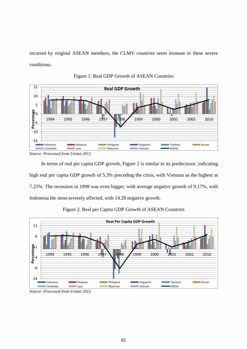
81

incurred by original ASEAN members, the CLMV countries seem immune to these severe

conditions.

Figure 1. Real GDP Growth of ASEAN Countries

Source: Processed from Unstat 2012

In terms of real per capita GDP growth, Figure 2 is similar to its predecessor, indicating

high real per capita GDP growth of 5.3% preceding the crisis, with Vietnam as the highest at

7.25%. The recession in 1998 was even bigger, with average negative growth of 9.17%, with

Indonesia the most severely affected, with 14.28 negative growth.

Figure 2. Real per Capita GDP Growth of ASEAN Countries


-15

-10

-5

0

5

10

15

1994 1995 1996 1997 1998 1999 2000 2001 2002 2010

Pe

rce

nta

ge

Real GDP Growth

Indonesia Malaysia Philippine Singapore Thailand Brunei

Cambodia Laos Myanmar Vietnam ASEAN

-14

-9

-4

1

6

11

1994 1995 1996 1997 1998 1999 2000 2001 2002 2010

Pe

rce

nta

ge

Real Per Capita GDP Growth



82

Looking at investment growth across the years of the crisis in Figure 3, before 1998,

ASEAN on average had very high annual GDP growth of 9.3%, with Myanmar as the highest

with 20.5%, and Malaysia (of ASEAN-6) by 14.1%. However, investment growth became

negative in 1998 at 30.5%, with Thailand as the most severely affected country, with 44%

negative investment growth. After recovering from the crisis, the average investment growth

was positive: 2% (1999-2002).

Figure 3. Investment Growth of ASEAN Countries


Trade balance was a component of economic balance; deterioration of the trade balance

could lead to a country‘s negative economic performance. Figure 4 shows that, on average

before the crisis, ASEAN suffered from a trade-deficit-to-GDP ratio of 0.6%. Brunei has the

highest surplus, 32.3%; by contrast, Laos has the biggest deficit, 20.6%.

During the economic crisis, in 1998, ASEAN had an average surplus of 4.5%. The

surplus increased after the crisis by an average of 6.4%, with Brunei still leading at 43%, and

Laos still the lowest, with a deficit of 14.8%. Miyakoshi (2000) noted two primary triggers of

the Asian crisis: current account deficits and significant progress in financial liberalization.

-45

-25

-5

15

35

55

75

1994 1995 1996 1997 1998 1999 2000 2001 2002 2010Pe

rce

nta

ge

Investment Growth

Indonesia Malaysia Philippine Singapore Thailand Brunei Cambodia Laos Myanmar Vietnam ASEAN

83

Figure 4. Trade Balance to GDP Ratio of ASEAN Countries


Traditionally, ASEAN members have had a high average inflation rate, as has been

shown in Figure 5. On average, prior to the 1998 crisis, the inflation rate was 8.7%. Among

CLMV countries, Myanmar had the highest inflation rate, at 23.8%. Of the original ASEAN

members, Indonesia had the highest at 8%. In 1998, the inflation rate soared dramatically,

especially in Indonesia, 58%, and Laos by almost 100%. After the crisis, generally, the

average inflation rate increased by 10%.

Figure 5. Inflation Rate of ASEAN Countries

Year-on-year change of the consumer price index, end of period Source: IMF, WEO 2012.

-25

-5

15

35

1994 1995 1996 1997 1998 1999 2000 2001 2002 2010Pe

rce

nta

ge

Trade Balance to GDP Ratio



0

50

100

1994 1995 1996 1997 1998 1999 2000 2001 2002 2010

Pe

rce

nta

ge

Inflation Rate



84

Figure 6 shows the interest rate conditions of ASEAN countries around the time of the

crisis. This figure confirms that the average interest rate before the crisis was 8.9%, and in

1999-2002 it decreased to 6.9%. In both periods, Indonesia had the highest interest rates at

16.6% and 17.3%; and responding high inflation rate in last 1997 and early 1998, it has the

highest interest rate in 1998 by 39%.

Figure 6. Interest Rate of ASEAN Countries

Deposit Interest Rate (%) Source: World Bank, WDI

Related to the nominal exchange rate, Figure 7 shows that before the crisis, Vietnam

had the least valued currency, in both before and after crisis by 11,180 and 14,528 over US$.

The strongest currency was held by Singapore and Brunei.

Figure 7. Nominal Exchange Rate of ASEAN Countries

LCU per US$, period average Source: Unstat 2012.

0

20

40

1994 1995 1996 1997 1998 1999 2000 2001 2002 2010

Pe

rce

nta

ge Interest Rate

Indonesia Malaysia Philippine Singapore Thailand BruneiCambodia Laos Myanmar Vietnam ASEAN

0

50

0

10,000

20,000

1994 1995 1996 1997 1998 1999 2000 2001 2002 2010

LCU

/US$

Exchange Rate

Malaysia Philippine Singapore Thailand BruneiMyanmar Indonesia Cambodia Laos Vietnam

85

Kho and Stulz (2000) argued that the Asian crisis was rooted primarily in financial

system vulnerabilities and other structural weaknesses; thus, a sharp depreciation of the

Indonesia rupiah had an adverse effect on Indonesian banks. Furthermore, Miyakoshi (2000)

showed that sharp depreciation of the local currency in 1998 was an indicator that relative

fixed exchange rates and high interest rates showed policy weakness.

Figure 8 shows that the deficit-to-GDP of ASEAN members was relatively low, -2.11%

in 1994-97 and -2.73 in 1999-2002; however, during the 1998 crisis, the deficit doubled.

Figure 8. Deficit-to-GDP Ratio of ASEAN Countries

General Government net lending/borrowing as percent of gross domestic product Resource: IMF, WEO 2012

Figure 9 shows that the debt-to-GDP ratio preceding the crisis was around 62.14%, but

increased to 64.9% after 1998. During the 1998 crisis, the average debt-to-GDP ratio was

70.1%, with Laos as the highest at 196.5%. Chan, Chao and Chuo (2002), also supported by

Kim (2001), argued that economies with trade similarities, and other parallel macroeconomic

fundamentals, are particularly susceptible to the contagion effect of rapidly spawning

currency attacks. This results in increasing economic uncertainty, decreasing public

-35

-25

-15

-5

5

15

1994 1995 1996 1997 1998 1999 2000 2001 2002 2010

Pe

rce

nta

ge

Deficit to GDP ratio



86

confidence in financial institutions, financial liberalization, and a reduction in the corporate

leverage ratio.

Figure 9. Debt-to-GDP Ratio of ASEAN Countries

General government gross debt as percentage of gross domestic product Source: WEO 2012.

Radelet and Sachs (2000) suggested that the Asian crisis was unpredictable.Capital

inflows remained strong, risk premiums were attached to loans to emerging market economies,

and assessments from credit-rating agencies and investment forecasts remained positive. The

conditions were supported by the fact that government debt was in surplus, domestic savings

and investment rates were very high, and world markets did not portend a crisis. However, the

crisis emerged in the 1990s, after risk expanded through current account deficits, overvalued

exchange rates, slowing export growth, and increasingly fragile financial institutions.

To investigate which countries in ASEAN suffered most acutely from the crisis, we

apply descriptive difference-in-difference analysis on various levels of economic performance

among ASEAN-6 members. Indonesia, Malaysia, Philippines, Singapore, Thailand, and

Brunei serve as as the treatment group; the CLMV countries—Cambodia, Laos, Myanmar,

and Vietnam—comprise the control group.

0

50

100

150

200

1994 1995 1996 1997 1998 1999 2000 2001 2002 2010

Pe

rce

nta

ge

Debt to GDP ratio

Indonesia Malaysia Philippine Singapore Thailand BruneiCambodia Laos Myanmar Vietnam ASEAN

87

The periods under examination were those before and after Asian crisis, from 1991 to

2004. As the peak of Asian crisis was in 1998, we established 1997 as the cut-off point.

Following Baskaran (2009), we measured effects using a descriptive DiD method on some

variables of interest (Q): growth in per-capita GDP, inflation and interest rates, deficit-to-

GDP and debt-to-GDP ratios, and trade balance-to-GDP ratio. The descriptive DiD equation

is set down in the following formula:

(4.1) DiD ASEAN=(QAS-6

98 –04 – QAS-6

91 – 97)–(QCLMV

98 – 04 – QCLMV

91 – 00)

Table 9 reports that the growth of real per-capita GDP of ASEAN-6 worsened after the

Asian crisis, in contrast with the performance improvements of CLMV; therefore, the pure

impact of the crisis was most painful for ASEAN-6. Related to inflation and interest rates,

although the per-capita GDP decreased for ASEAN-6, it was lower in comparison with

CLMV members.

Table 9. Descriptive DiD Results: The Impact of the Asian Crisis on Original ASEAN States:

1991–2004

GGDPC Inf Int ER Def Debt TB

ASEAN -6

Post-Crisis 1.43 4.60 6.65 1525.12 -1.81 51.66 15.37

SD 0.78 6.36 5.85 3688.48 3.71 30.23 17.11

N 42 42 42 42 42 42 42

Pre-Crisis 4.86 5.19 8.97 384.27 0.32 44.81 7.16

SD 2.31 2.84 5.41 912.58 10.41 24.29 14.88

N 42 42 42 42 42 42 42

Difference -3.43 -0.59 -2.32 1140.85 -2.13 6.85 8.21

CLMV

Post-Crisis 5.31 18.94 7.81 6854.62 -3.81 82.18 -7.21

SD 4.45 18.50 2.73 6114.53 1.41 45.75 6.06

N 28 28 28 28 28 28 28

Pre-Crisis 2.75 26.52 11.07 3494.17 -4.46 116.29 -9.27

SD 2.11 16.22 3.77 5044.65 2.24 47.58 7.62

N 28 28 28 28 28 28 28

Difference 2.56 -7.59 -3.26 3360.45 0.65 -34.11 2.07

Diff-in-diff -5.99 7.00 0.94 -2219.61 -2.78 40.96 6.14

Note: Pre-Crisis was from 1991 to 1997 and Post-Crisis was from 1998 to 2004.

Source: Author’s calculation

88

Thus, the pure impact of the crisis was still negative. ASEAN countries have employed

an outward-looking strategy, so the depreciation of currency, although not as sharp as during

the crisis, was beneficial in inducing higher exports. The currency depreciation was higher in

CLMV by comparison with ASEAN-6; however, recent currency conditions might be

desirable for ASEAN-6.

Related to fiscal conditions, the deficit-to-GDP ratio rose in ASEAN-6 countries by

2.13, but declined in CLMV; debt-to-GDP ratio was in line with deficit values. Thus, the

fiscal performance deteriorated in ASEAN-6 in after crisis period.

Finally, we evaluated trade balance figures. Although sharp depreciation, mainly in

Indonesia, the Philippines, Malaysia, and Thailand, shocked economic performance, the

general impact on export performance was positive. Table 9 confirms that the trade surplus in

ASEAN-6 was improving by 8.2%, which is higher than the improvement in CLMV, 2.1%.

From these figures, we might conclude that the Asian crisis in 1998 was mainly incurred by

ASEAN-6 countries.

This finding was in line with Sarno and Taylor (1999), who showed that of ASEAN

members, Indonesia, Malaysia, the Philippines, and Thailand had more severe conditions, due

to bursting asset price bubbles fostered by strong capital inflows, moral hazard problems, and

a vicious cycle of asset price deflation.

Radelet and Sachs (2000) suggested different causes for the severity of the crisis in Asia,

as shown in figure 3:

Large-scale, unanticipated, involved, unguaranteed lending to debtors, leading to lack of

credit for viable enterprises

89

Positive market reaction to initiate that bring creditors and debtors together for orderly

workouts

Triggering events leading to the sudden withdrawal of investor funds.

Wade (1998) demarcated four steps in the chronology of the Asian crisis: the exchange

collapse; the upsurge of bank failures and company bankruptcies resulting from the

unavoidable costs of un-hedged foreign debt; a domestic recession resulting from falls of

consumption and investment, combined with rising unemployment; and political reaction

from the slump. It began with inflationary pressure from the combination of financial capital

inflows and fixed exchange rate regimes, ultimately resulting in the property bubble burst of

1995 and the stock market crash of 1996.

According to Radelet and Sachs (2000), the Asian crisis would not have been so severe

developed countries mainly Japan and USA commit to help more and the process of financial

liberalization was slower. Radelet and Sachs (2000) also summarized the five inherent

characteristics of a financial crisis: (1) a macroeconomic policy-induced crisis, (2) a financial

panic, (3) a bubble collapse, (4) a moral hazard crisis, and (5) a disorder workout. Kaminsky

and Reinhart (1998) pointed out that the Asian crisis occurred as economies entered a

recession that followed a prolonged boom in economic activity, which had been fueled by

credit creation and surges in capital inflow.

These conditions were supported by the fact that government debt was in a surplus state

(Fig. 9), domestic savings and investment rates were very high (Fig. 3), and the world market

did not portend a crisis. However, the crisis emerged after risk grew: throughout the 1990s,

there had been growth in current account deficits (Fig. 8), an overvalued exchange rate (Fig.

90

7), slowing export growth (Fig. 4), and increasingly fragile financial institutions. According to

Tse (2001), historically, financial crashes occur when everything seems to be going well—

when economic growth is strong, inflation is low, and optimism is high. In 1997, The

contagion effect of the crisis finally spread in East and Southeast Asia.

Palley (2011), following the Minskian framework, hypothesized that the crisis resulted

from an unstable economic process under financial capitalism. Stiglitz (2000), meanwhile,

believed that capital market liberalization was responsible for the Asian crisis, since it mainly

produces instability, rather than growth. In this vein, Minsky (1977) emphasized the

importance of adequate government constraints on institutions to stabilize the economy.

4.4 Identifying the Crisis in the Eurozone

Various arguments have been made to explain the Eurozone crisis. Perez-Caldentey and

Vernengo (2012) argued that the original source of the crisis in the Eurozone is domestic debt,

combined with self-fulfilling expectations and financial sector imbalances. Based on the

Keynesian framework, the inability to contain labor cost growth within Europe‘s peripheries

led to a loss of competitiveness; furthermore, they argued that more and more external

problems have combined with the financial crisis, resulting in a collapse of output, and finally,

fiscal crisis. The competitiveness problem festered, as there was no depreciation mechanism

with respect to nominal exchange rates, and there was an absence of supranational fiscal

authority that could otherwise transfer resources.

Germany‘s mercantilistic behavior—characterized by the maintenance of a foreign trade

surplus, being non-cooperative at the global and European levels, and relying on domestic

price stability and export-led growth—was accused of contributing to the crisis (Bellofiore,

91

Garibaldo and Halevi 2010). The European crisis led to a devaluation of the Euro, which

improved German export competitiveness; ultimately, Germany profited from its neighbors‘

sacrifice.

The peripheries could not reinforce their economies, due to a fiscal-tightening policy that

was meant to maintain price stability, but led to an inability to fully control monetary policy.

Germany‘s behavior has been consistent with neo-mercantilism (Cesaratto and Stirati 2011),

which includes taking advantage of a fixed exchange rate to increase exports, by pursuing a

domestic inflation rate lower than competitors; relying on other countries‘ stimuli to promote

demand; taking advantage of ensuing inflationary bias, while compensating with conservative

domestic fiscal (and monetary) policy; and responding to foreign critics by blaming their lack

of discipline.

Low wages induced a depressed domestic market and encouraged firms to find external

markets, thus generating export hypertrophy. The combination of trade surplus (as a result of

an export-led growth strategy), wage moderation, and domestic demand compression gave

Germany a long-term advantage over its competitors (Whyte 2010). Regardless of their size

in 1980–2010, the peripheries‘ existence could not be ignored, since any crisis in a small

country like Greece or Ireland could have a contagion effect on others.

Regarding population, the peripheries‘ share was 40% of the Eurozone‘s (308 million

total), larger than their proportion of the GDP. Italy has the biggest share of population

(18.7%), while Ireland has the smallest (1.2%); Germany, meanwhile, accounts for 26.2% of

the Eurozone population. Clearly, the peripheries‘ share of population is not aligned with their

share of GDP within the union.

92

Figure 10. Size of Peripheries: Real GDP and Population (Eurozone = 100)

Note: In percentage; GDP is 2005 constant prices in USD. Source: Unstat.

Figure 11 compares the development of real per-capita GDP between the peripheries and

Germany. In 1980, the average per-capita income in the peripheries was 76% lower than the

Eurozone (91.6%). Italy‘s (90.6%) was higher than the other peripheries, followed by Ireland

(81.2%). Portugal was the poorest country of the peripheries, with only 45% of Germany‘s

per-capita GDP.

A surprising change occurred in 2000, when Ireland (USD42,007) overtook Germany

(USD32,608) by 28.8% in terms of per-capita GDP. In 1980, there was virtually no difference

between the peripheries and Germany, in terms of productivity. In that year, Italy‘s

productivity was the highest, at 115% of Germany‘s. In 1990, Italy and Spain were still

stronger than Germany (by 14% and 2.1%, respectively). Ireland‘s huge leap occurred in 2010,

when its productivity skyrocketed from 77% to 120% of Germany‘s. Portugal had the lowest

position for four decades, around 60% of German productivity.

High per-capita GDP and productivity were supported by high growth rates, as shown in

Figure 20. Ireland enjoyed a 94.4% growth rate relative to Germany, along with a 3.1%

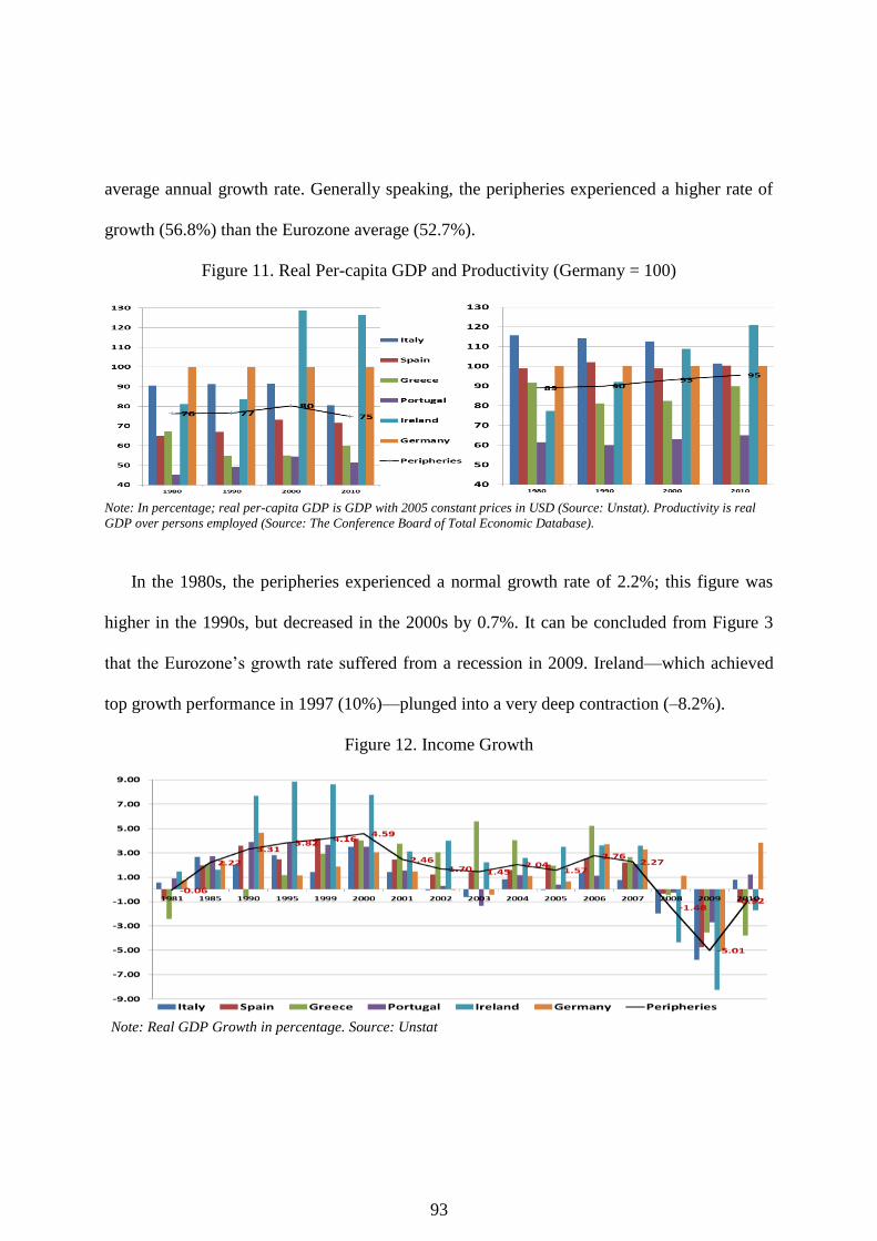
93

average annual growth rate. Generally speaking, the peripheries experienced a higher rate of

growth (56.8%) than the Eurozone average (52.7%).

Figure 11. Real Per-capita GDP and Productivity (Germany = 100)

Note: In percentage; real per-capita GDP is GDP with 2005 constant prices in USD (Source: Unstat). Productivity is real

GDP over persons employed (Source: The Conference Board of Total Economic Database).

In the 1980s, the peripheries experienced a normal growth rate of 2.2%; this figure was

higher in the 1990s, but decreased in the 2000s by 0.7%. It can be concluded from Figure 3

that the Eurozone‘s growth rate suffered from a recession in 2009. Ireland—which achieved

top growth performance in 1997 (10%)—plunged into a very deep contraction (–8.2%).

Figure 12. Income Growth

Note: Real GDP Growth in percentage. Source: Unstat

94

Spain has had the highest average unemployment rate in the Eurozone (17.8%). The other

peripheries have also experienced persistently higher unemployment rates compared to the

core Eurozone countries.

In 1983, Ireland followed Spain in experiencing a high level of unemployment (14.7%).

According to Bentolila and Cahuc (2010), Spain‘s high unemployment rate was caused by a

large gap in firing costs between permanent and temporary contracted workers, the absence of

free collective use among temporary contracts, and the high availability of low-skilled jobs

through very flexible contracts and a huge inflow of low-skilled immigrants.

Figure 13. Unemployment and Youth Unemployment Rates

Note: In percentage (WDI); unemployment: share of the labor force that is without work but available for and

seeking employment. Youth unemployment refers to unemployment among those aged 15–24.

In 1993, Spain‘s unemployment rate exceeded 20%, followed by Ireland at 15.7%.

Portugal, on the other hand, enjoyed the lowest rate of unemployment (5.13%). In 2003,

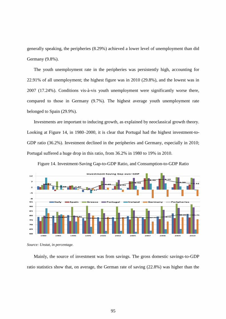
95

generally speaking, the peripheries (8.29%) achieved a lower level of unemployment than did

Germany (9.8%).

The youth unemployment rate in the peripheries was persistently high, accounting for

22.91% of all unemployment; the highest figure was in 2010 (29.8%), and the lowest was in

2007 (17.24%). Conditions vis-à-vis youth unemployment were significantly worse there,

compared to those in Germany (9.7%). The highest average youth unemployment rate

belonged to Spain (29.9%).

Investments are important to inducing growth, as explained by neoclassical growth theory.

Looking at Figure 14, in 1980–2000, it is clear that Portugal had the highest investment-to-

GDP ratio (36.2%). Investment declined in the peripheries and Germany, especially in 2010;

Portugal suffered a huge drop in this ratio, from 36.2% in 1980 to 19% in 2010.

Figure 14. Investment-Saving Gap-to-GDP Ratio, and Consumption-to-GDP Ratio

Source: Unstat, in percentage.

Mainly, the source of investment was from savings. The gross domestic savings-to-GDP

ratio statistics show that, on average, the German rate of saving (22.8%) was higher than the

96

peripheries (19%). In 1980, Portugal achieved the highest rate of saving (31%), but it dropped

sharply in 2010, to only 9%. These conditions are similar to those seen in Ireland, which had a

rate of saving of 19% in 1980, achieved its peak in 2000, but dropped to 11.5% in 2010. The

conditions in Greece were very bad, where the savings ratio started at 21% in 1980, but

dropped continuously until it bottomed out at 4.1% in 2010.

High investment in the peripheries was driven by speculative motives: large capital

inflows in 2002–07 (Figure 14), were quickly fueled by high growth, which had, in turn, been

driven by strong demand for consumption and construction investment. Capital was financed

easily by credit from abroad. When the crisis exploded—especially as investments had not

financed productive sectors—these countries needed to repay their debts, but in the absence of

the support of previous investments. Thus, investment directed to consumption rather than

production had contributed to inflated bubbles that produced temporary, but ultimately

unsustainable, nominal growth.

Financial deficits in Greece, Portugal, and Spain correlated with the collapse of savings,

especially in 2010. Figure 14 shows that, among the peripheries, Greece had the highest

consumption-to-GDP ratio. Ireland has been most effective at lowering its consumption-to-

GDP ratio, and thus, has had the lowest consumption-to-GDP ratio in the Eurozone since the

1990s, even compared to Germany.

Generally speaking, from the 1980s until the early 2000s, the consumption-to-GDP ratios

of the peripheries were lower than that of Germany, but after the 2000s, things changed. With

respect to the trade balance-to-GDP ratio (Figure 15), in 1980, Spain and Italy enjoyed high

surpluses (7.7% and 4.8%, respectively), but the other peripheries suffered from deficits. Italy

97

enjoyed a surplus in 1980, but suffered a deficit in 2010 (–13.64%). Greece suffered persistent

trade deficits, starting with –2.7% in 1980, and later, –20.9% in 2010. By contrast, Germany

and Ireland started with deficits but later had surpluses. The peripheries were showing trends

of growth vis-à-vis international trade. Unfortunately, after the 2000s, the growth of imports

exceeded that of exports, in contrast with the conditions in Germany.

Figure 15. Trade Balance-to-GDP Ratio

Note: Export–Import over GDP, in percentage. Source: Unstat.

We might address the issue of competitiveness to explain trade phenomena; these

phenomena cab be explained in terms of the cost of production, or unit labor cost, as implied

by Cesaratto and Stirati (2011).

In 1980–2010, the average growth of unit labor cost in Germany (1.55%) was very low

compared to the peripheries (6.7%). Among the peripheries, Greece had the highest growth

(10.6%) and Ireland (3.98%) the lowest. Germany‘s strong performance, according to Vines

(2011), derived from its ability to pursue wage moderation and restraint policies vis-à-vis

labor costs. The peripheries did not have the same mechanisms to counteract Germany‘s

98

actions—actions which, in Germany, had compensated for the loss of output associated with a

decline in competitiveness.

Figure 16. Growth of Unit Labor Cost

Note: Total economy unit labor cost (index 2005 = 100). Source: OECD statistics. Measures of the average cost

of labor per unit of output are calculated as the ratio of total labor costs to real output.

Level of trade competitiveness is determined not only by the cost of labor, but also by

exchange rates. Since all Eurozone members fully surrendered their own currencies and

monetary policies to the ECB to make use of the Euro, they became unable to devalue or

depreciate their currency to enhance competitiveness.

Figure 17. Real Exchange Rate

Source: Unstat & WDI, RER = a*b, where a = Nominal exchange rate and b = US CPI/Domestic CPI. After

2002, only b was different among countries.

Figure 17 shows that Germany‘s real exchange rate has always been higher than the

peripheries, which might explain why Germany has had trade surpluses while the peripheries

99

had deficits. The combination of low growth in unit labor costs and a lower real exchange

rate—especially in comparison to the peripheries, as implied by Lapavitsas et al. (2010a)—

has helped Germany enjoy a trade surplus supported by its competitiveness and the

peripheries‘ economic sacrifice.

To clarify the importance of the MC in stabilizing the Eurozone, we divided our period

under analysis into two subperiods: the years before the introduction of the euro in 1999, as

the final stage of monetary union realization, and the time around the Eurozone crisis.

Table 10. Maastricht Criteria and Peripheries: Prior to euro Introduction

MC Italy Spain Greece Portugal Ireland Germany

Inflationa

1996 2.65 3.97* 3.56* 8.20* 3.12* 1.69 1.45

1997 2.76 2.04 1.97 5.54* 2.16 1.44 1.88

1998 2.32 1.96 1.83 4.77* 2.72 2.43 0.94

Interestb

1996 4.90 6.49* 6.12* 13.51* 6.32* 0.29 2.83

1997 5.00 4.83 3.96 10.11* 4.56 0.46 2.69

1998 4.91 3.16 2.92 10.70* 3.37 0.43 2.88

Deficitc

1996 -3.00 -6.96* -4.85* -6.79* -2.87 -0.11 -3.33*

1997 -3.00 -2.68 -3.39* -6.02* -1.69 1.43 -2.65

1998 -3.00 -3.07* -3.21* -3.91* -1.77 2.24 -2.18

Debtc

1996 60.00 113.62* 56.06 101.60* 61.29* 64.70* 22.88

1997 60.00 110.95* 55.28 105.22* 56.24 57.31 24.25

1998 60.00 108.72* 53.56 103.75* 52.99 47.8 26.06 Note: a. Calculated by summing average inflation rate of three lowest inflation rate countries in 1996–98 plus 1.5%; b. Calculated by summing average long-term interest rates in these three low-inflation countries in 1996–98 plus 2%; c.

The exact number determined in Maastricht Treaty; and * Indication of inability to meet the criterion.

The main reason that Greece‘s membership application was rejected in 1998 was that the

country had been unable to meet the MC in 1996–98. Similarly, Italy, Portugal, and Spain

failed to meet the inflation criterion in 1996. Concerning the fiscal criteria, Italy had failed to

control its finances, Spain had been unable to meet the deficit criterion, and Ireland and

100

Portugal followed Germany in meeting almost all criteria required to become an EMU

member.

As a retest of conditions in 2007–09, Table 30 shows that Greece met only the interest

rate criterion; Greece was far from satisfying fiscal criteria, as its public debt was twice that

allowed by the MC, and its deficit was five times higher than the MC criteria. Portugal failed

to meet deficit and debt criteria, and Italy failed to meet the debt criterion. Finally, Ireland and

Spain had huge deficit problems in 2009.

Table 11. Maastricht Criteria and Peripheries: Prior to 2009 Eurozone Crisis

MC Italy Spain Greece Portugal Ireland Germany

Inflationa

2007 3.14 1.82 2.79 2.9 2.81 4.88* 2.29

2008 4.07 3.38 4.07 4.15* 2.59 4.05 2.63

2009 1.07 0.75 -0.4 1.21* -0.83 -4.48 0.31

Interestb

2007 6.31 4.49 4.31 4.5 4.42 4.33 4.22

2008 6.24 4.68 4.36 4.8 4.52 4.55 3.98

2009 6.00 4.31 3.97 5.17 4.21 5.23 3.22

Deficitc

2007 -3.00 -1.49 1.898 -6.69* -3.15* 0.08 0.26

2008 -3.00 -2.69 -4.15* -9.80* -3.54* -7.34* 0.12

2009 -3.00 -5.30* -11.13* -15.51* -10.11* -14.20* -3.06*

Debtc

2007 60.00 95.63* 30.02 105.67* 66.62* 19.83 39.55

2008 60.00 98.09* 33.70 110.62* 68.88* 28.00 39.55

2009 60.00 106.78* 46.03 127.02* 78.73* 47.07 44.21 Note: a. Calculated by summing average inflation rate of three lowest inflation rate countries in 1997–99 plus 1.5%; b.

Calculated by summing average long-term interest rates in these three low-inflation countries in 1997–99 plus 2%; c. The exact number determined in the Maastricht Treaty; and * Indication of inability to meet the criterion.

The ECB was successful in its monetary role, keeping interest rates and inflation low.

Vines (2011) implies that the process of euro adoption, starting from January, 1 1999, led to

rapid cross-border flows of finance and induced inflation and interest rate convergence.

Unfortunately, Greece, Italy, and Portugal each had large fiscal deficits and very high debt-to-

GDP ratios, prompting discretionary policy action.

101

The inability to meet fiscal MC criteria was one of the main causes of the recent crisis in

the peripheries. As the governments were compelled to increase expenditures to mitigate the

impact of the crisis—even as revenues concurrently declined—budget deficits were inevitable

and emerged as a frequently cited cause of the debt crisis.

The success of the ECB in fulfilling its monetary duties fueled a credit boom in 2003–07,

which increased business-cycle fragility. The credibility of the ECB on inflation targeting and

the Euro was seen at a stable currency and optimism in the financial market. Investments

soared as currency risk dramatically diminished and competition boosted financial innovation,

as firms and financial institutions could borrow easily from abroad.

Investment growth in the peripheries concentrated mainly in the housing sector, boosting

rapid growth, and credit growth translated into a build-up of debt. Faster growth experienced

by the peripheries induced consumption, fed demand for imports, and led to a larger current

account deficit. Thus, the twin deficits suffered by Greece finally led the country to a 15.5%

budget deficit-to-GDP ratio and a 127% debt-to-GDP ratio in 2009. For these reasons, Greece

suffered high external debt, and a low rate of national savings plunged the country into a

sovereign debt problem.

Ireland has been an inspiring success story since the late 1990s. Its transformation from a

poor country lacking natural resources to an affluent country was evidenced by its dramatic

growth in terms of per-capita GDP, from USD23,420 in 1990 to USD52,472 in 2007.

Improvements, according to Anand, Gupta, and Dash (2012), were due to intensified global

economic activity, as well as the state‘s policy of encouraging the attainment of high-level

skills and attracting investment in high technology companies.

102

Table 12. Summary of Crisis Indicator in Peripheries

Country Condition Crisis Indicator Type of Crisis*

Greece High growth in 2000s Negative growth BOP crisis

Traditional trade deficit country –15.5% and 127% deficit and debt-to-GDP ratio Bubble collapse

Growth come from consumption High unemployment Moral hazard

Unable to satisfy MC Low real exchange rate

High ULC growth High trade deficit

Ireland High growth induced by investment post-

1990s

Private sector crisis translated into fiscal stress Bubble collapse

–14.2% deficit-to-GDP ratio Financial panic

High unemployment

Recession, –8% real GDP growth

Spain Traditionally high unemployment High general and youth unemployment (20% and

40%)

BOP crisis

Private sector crisis translated into fiscal stress Bubble collapse

–11.3% deficit-to-GDP ratio

High trade deficit

Portugal Lowest per-capita GDP –9.14% and 87.9% deficit and debt-to-GDP ratio BOP crisis

High consumption High deficit trade balance Bubble collapse

Deficit trade country High unemployment

High growth of ULC Low productivity

Italy Chronic low growth –4.5% and 109% deficit and debt-to-GDP ratio BOP crisis

8th highest GDP in world –13.6% high trade deficit-to-GDP ratio

Changing pattern from surplus to deficit trade

Note: *Crisis typology based on Radelet and Sachs (2000).

High economic growth led to a rapid expansion in credit and property valuation, but in the

absence of sufficient control of the private sector, there was an increase in mortgages,

accompanied by the banks‘ overreliance on wholesale external borrowing (i.e., financial

fragility), as predicted by Minsky‘s hypothesis (Palley 2011). Therefore, the property price

crash in Ireland in 2007 resulted from losses in the banking sector (Avellaneda, Dellepiane

and Hardiman 2010). Clearly, a government cannot overcome such large losses without

outside support.

Spain‘s low rates of inflation and interest attracted significant foreign investment,

especially in the real estate sector, which accounts for 16% of its GDP (Anand, Gupta and

Dash 2012). The real estate price collapse in 2007 caused a significant increase in personal

debt. The decline in government tax revenue caused a dramatic increase in the deficit-to-GDP

103

ratio, from –0.86% in 2000 to –5.30% in 2009. Fortunately, its debt-to-GDP ratio (51.7% in

2010) was lower than that demanded by the MC.

As implied by Gros and Alcidi (2011), the main problem in Spain was the dependence of

Spanish banks on foreign finance, accompanied by the structural problem of a persistently

high unemployment rate, which has always been in excess of 10%. Spain, even with its lower

debt and higher rate of savings, plunged into crisis, and financial activities within the country

faced serious liquidity problems.

The financial crisis in Portugal can be viewed in terms of a deterioration in the debt-to-

GDP ratio, from 54% in 2002 to 87.9% in 2010, as well as a sharp fiscal deficit plunge, from

–0.36% in 2007 to –9.14% in 2010. Although the country experienced an investment boom in

the 1990s—leading to a 5.5% rate of growth—after the euro was launched, Portugal suffered

from annual negative investment growth (–2.9%). A significantly large external current

account deficit and external debt have been fueled largely by a combination of private sector

borrowing, low productivity, high unemployment rates, and high growth in unit labor costs.

Portugal, therefore, has a complicated economic problem that features a low rate of national

saving—a problem that has manifested as insolvency and a sovereign debt problem.

The contagion effect of the crisis will become even more serious if it reaches Italy, due to

that country‘s economic size. Among the peripheries, Italy had the lowest annual per-capita

GDP growth (1.1%) in 1980–2010. Low growth, a high deficit (–4.5% in 2010), and a high

debt-to-GDP ratio (109% in 2010) has pushed the country into recession. The problem was

exacerbated by its high trade deficit (–13.6% in 2010).

104

Traditionally, Italy has been able to create surplus foreign trade by devaluing its currency,

and thus maintaining its competitiveness (Bellofiore and Halevi 2011), but by surrendering

the lira and the authority to devaluate the common currency it shares, Italy has been unable to

maintain its competitiveness, largely because it has been unable to maintain labor costs at a

level as low as Germany‘s. Fortunately, Italy had a high saving rate, which helped alleviate

problems relating to its huge public debt.

4.5 Difference-in-Difference Analysis

To investigate the causal impact on the peripheries of the release of the Euro, we applied

the DiD method, which is widely applied in empirical work to establish the causal effect of a

given nonrandom policy intervention.

Table 13. Definitions and Source of Variables

Name Definition Source

Dependent variables

GGDPC Growth of GDP/population Unstat, National Accounts Main Aggregate (SNA) Database

GLP Growth of GDP/persons employed Conference Board Total Economy Database

Unemp Ratio of unemployment/labor force World Bank, WDI

Inf Percentage-change in consumer price index World Bank, WDI

Int Long-term interest rate OECD statistics

Def Revenue–expenditure-to-GDP ratio OECD statistics

PD Public debt-to-GDP ratio OECD statistics

TB Export–Import to GDP ratio Unstat, SNA Database

Institutional variables

DI Dummy = 1 if time of euro introduced is 2001–10 Author‘s calculations

DP Dummy = 1 if belong to peripheries Author‘s calculations

DE Dummy = 1 if in peripheries and in 2001–10 Author‘s calculations

DK Dummy = 1 if time of crisis in 2007–10 Author‘s calculations

Exogenous control variables

Open Export + import-to-GDP ratio Unstat, SNA Database

K Gross of fixed capital formation/GDP Unstat, SNA Database

WA

Percentage of population aged 15–64/total

population World Bank, WDI

Pop Logarithm of population Unstat, SNA Database

ULC Growth of unit labor cost OECD statistics

As a treatment group, we investigated the various levels of economic performance among

the peripheries (Italy, Spain, Greece, Portugal, and Ireland), as countries with the euro as a

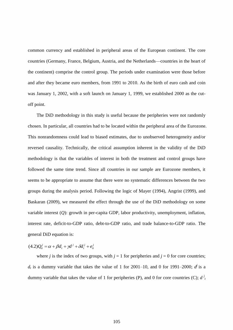
105

common currency and established in peripheral areas of the European continent. The core

countries (Germany, France, Belgium, Austria, and the Netherlands—countries in the heart of

the continent) comprise the control group. The periods under examination were those before

and after they became euro members, from 1991 to 2010. As the birth of euro cash and coin

was January 1, 2002, with a soft launch on January 1, 1999, we established 2000 as the cut-

off point.

The DiD methodology in this study is useful because the peripheries were not randomly

chosen. In particular, all countries had to be located within the peripheral area of the Eurozone.

This nonrandomness could lead to biased estimates, due to unobserved heterogeneity and/or

reversed causality. Technically, the critical assumption inherent in the validity of the DiD

methodology is that the variables of interest in both the treatment and control groups have

followed the same time trend. Since all countries in our sample are Eurozone members, it

seems to be appropriate to assume that there were no systematic differences between the two

groups during the analysis period. Following the logic of Mayer (1994), Angrist (1999), and

Baskaran (2009), we measured the effect through the use of the DiD methodology on some

variable interest (Q): growth in per-capita GDP, labor productivity, unemployment, inflation,

interest rate, deficit-to-GDP ratio, debt-to-GDP ratio, and trade balance-to-GDP ratio. The

general DiD equation is:

where j is the index of two groups, with j = 1 for peripheries and j = 0 for core countries;

dt is a dummy variable that takes the value of 1 for 2001–10, and 0 for 1991–2000; dj is a

dummy variable that takes the value of 1 for peripheries (P), and 0 for core countries (C); d jt

j

it

j

t

j

t

j

it edddQ )2.4(

106

is an interaction dummy that takes the value of 1 for P and in period 2001–10, and 0

otherwise; is the coefficient for C and in 1991–2000; is the coefficient for the dummy

period; is the coefficient value for the dummy group; is the coefficient value for the

interaction dummy group and period (DiD coefficient); and ejit is an error term. The DiD

result can be calculated by using the following formula:

(4.3) (QP

01 – 10 – QP

91 – 00)–(QC

01 – 10 – QC

91 – 00) = ( + )–() = .

We also calculated descriptive DiD for recent conditions in the Eurozone, by using the

following formula:

(4.4) (QP

07 – 10 – QP

01 – 06) – (QC

07 – 10 – QC

01 – 06) = (` + `) – (`) = `.

The DiD estimation is usually determined by regression. The advantages thereof include

the ease of obtaining final estimates, calculating the standard error, or extending the model to

cover more periods, treatments, or additional covariates, without expending much more

computational effort. In this way, the residual variance may be reduced (Meyer 1994). Since

descriptive calculations can offer only preliminary evidence, we re-estimate with the

following model:

itit

eDEDPDIQ itit 5.4 ,

where DI is a dummy that takes the value of 1 for the 2001–10 period, and 0 otherwise;

DP is a dummy variable that takes the value of 1 for peripheries, and 0 otherwise; and DE is a

categorical interaction variable that takes the value of 1 for peripheries and in 2001–10 period,

and 0 otherwise. The estimated coefficient is identical to the estimated coefficient in

equations (4.2) and (4.3). Since many unobservable, country-specific factors (e.g.,

107

geographical position, climate, and technological progress) could correlate with the error term,

ordinary least squares (OLS) results might be biased; thus, we apply the fixed-effect

approach:

itit

eDEQ itti 6.4 ,

where i is country fixed effects, and t is the year fixed effect. The DP and DI dummies

are dropped from this specification, due to perfect collinearity with subsets of the country and

year fixed effects. Since we have a vector of characteristics for each country under

examination, we augmented them as additional vectors of explanatory variables. Thus, the

OLS equation is:

itit

exdkDEDPDIQ kitktitit 7.4 ,

where dk is a dummy for the Eurozone crisis, and it takes the value of 1 for 2006–07, and

0 otherwise; and x (1, 2, …, k) are control variables, as described in Table 5. Equation (7.6)

provides us with a simple way of adjusting differences between the observations in the two

groups. Using this equation may also improve the efficiency of estimation by reducing the

residual variance. The inclusion of explanatory variables might assist in detecting omitted

variables or functional form misspecifications that could otherwise render regression

adjustments inadequate. In fixed-effect regression, the equation is:

itit

exdkDEQ kitktitti 8.4 .

4.6 Result

Table 33 reports that the growth of real per-capita GDP and labor productivity in the

peripheries worsened after the euro was introduced. With the exception of slower growth in

108

per-capita GDP and the deterioration of trade balances, other indicators were more promising.

Following the introduction of the Euro, core countries had higher per-capita GDP growth

figures and lower unemployment rates, but lower labor productivity growth.

Table 14. Descriptive DiD Results: The Impact of the euro on Peripheries in 1991–2000 GGDPC GLP Unemp Inf Int Def Debt TB

Peripheries

Post-Euro (+++) 0.60 0.84 8.63 2.65 4.28 -4.23 70.40 -6.29

N 50 50 50 50 50 50 50 50

Pre-Euro (+) 2.82 1.98 11.41 4.89 7.06 -4.25 75.24 0.83

N 50 50 50 50 50 50 50 50

Difference (+) -2.22 -1.13 -2.78 -2.24 -2.78 0.02 -4.84 -7.12

Core countries

Post-Euro (+) 0.87 0.65 6.64 1.86 3.92 -2.34 58.62 4.18

N 50 50 50 50 50 50 50 50

Pre-Euro () 1.96 1.51 7.46 2.19 3.77 -3.29 57.26 1.52

N 50 50 50 50 50 50 50 50

Difference () -1.09 -0.86 -0.82 -0.33 0.16 0.95 1.36 2.66

DiD () -1.13 -0.27 -1.96 -1.91 -2.93 -0.93 -6.20 -9.78

Note: “Post-Euro” is 2001–10, and “Pre-Euro” is 1991–2000.

The peripheries, on the other hand, followed trends consistent with inflation and deficit.

Adjustments to the MC can cause increases in interest rates and debt-to-GDP ratios. While the

peripheries suffered from very large trade deficits, the core countries enjoyed growing trade

surpluses. The results indicate that the peripheries received benefits upon embracing the Euro,

in the form of lower unemployment rates, inflation rates, interest rates, and deficit- and debt-

to-GDP ratios. Unfortunately, growth in per-capita GDP, labor productivity, and trade

balances worsened.

Suspecting that the peripheries experienced deterioration in some key indicators in 2007–

10, we applied equation 4.4 (Table 15). Not only had the growth of per-capita GDP and labor

productivity worsened during the crisis period, but also, variables associated with MC: either

unemployment or interest rates were increasing, and there was considerable deterioration in

109

deficit- and debt-to-GDP ratios, and trade balances. The pure effect showed that the crisis

occurred mainly in the peripheries in terms of per-capita GDP growth, unemployment, deficit

and debt-to-GDP ratios, and trade balances.

Table 15. Descriptive DiD Results: The Impact of Crisis on Peripheries in 2001–10 GGDPC GLP Unemp Inf Int Def Debt TB

Peripheries

Postcrisis (`+`+`+`) -1.68 0.60 9.83 1.92 4.83 -7.92 76.00 -7.88

N 20 20 20 20 20 20 20 20

Precrisis (`+`) 2.12 1.01 7.83 3.14 3.92 -1.77 66.67 -5.24

N 30 30 30 30 30 30 30 30

Difference (`+`) -3.80 -0.41 2.00 -1.23 0.92 -6.15 9.33 -2.65

Core countries

Postcrisis (`+`) 0.37 0.03 6.35 1.75 3.82 -2.95 60.30 4.58

N 20 20 20 20 20 20 20 20

Precrisis (`) 1.21 1.07 6.84 1.94 3.99 -1.93 57.50 3.91

N 30 30 30 30 30 30 30 30

Difference (`) -0.83 -1.05 -0.50 -0.19 -0.17 -1.02 2.80 0.68

DiD (`) -2.97 0.64 2.50 -1.04 1.09 -5.13 6.53 -3.32

Note: “Post-crisis” is 2007–10, and “pre-crisis” is 2001–06.

Table 16 indicates that the signs and coefficients of the DiD estimation (indicated by DE)

are identical to those derived through descriptive calculations (Table 14).

Table 16. The Impact of euro on Economic Variables (OLS Model)

GGDPC GLP Unemp Inf Int Def Debt TB

C () 1.9610* 1.5028* 7.4620* 2.1920* 3.7658* -3.2922* 57.2626* 1.5156*

DI () -1.0890 -0.8534*** -0.8180** -0.3304 0.1556 0.9520 1.3582 2.6604*

DP () 0.8604*** 0.4122** 3.9520* 2.6946* 3.2952* -0.9622** 17.9790* -0.6876

DE () -1.1312 -0.3242 -1.9640* -1.9062* -2.9350* -0.9274 -6.2022* -9.7834*

N 200 200 200 200 200 200 200 200

F 7.2466 7.7248 16.8450 19.5003 14.0405 2.8330 5.0396 13.3539

R2 0.0861 0.0920 0.1928 0.2181 0.1643 0.0269 0.0574 0.1570

Note:*, **, and *** indicate significance at the 1%, 5%, and 10% significant levels, respectively.

To check for robustness and preclude heterogeneity, we applied a fixed-effect estimation.

The results confirmed the robustness of the signs of the variables of interest, save that the

influence of the euro on reducing growth in per-capita GDP, productivity, and debt was found

110

to be insignificant. The deficit-to-GDP ratio result was inconclusive, due to insignificance

within both models.

Table 17. The Impact of euro on Economic Variables (Fixed Effects Model)


DE (̀ )̀ -2.2202*** -1.1776* -2.7820* -2.2366* -2.7794* 0.0246 -4.8440 -7.1230*

N 200 200 200 200 200 200 200 200

F 3.2656 3.1493 38.6847 11.5749 14.1787 3.4949 109.2464 22.5935

R2 0.1022 0.0975 0.6544 0.3470 0.3984 0.1114 0.8447 0.52041


With additional control variables, the OLS estimation results in Table 18 obviously

confirm our previous results: the euro had an insignificant effect on the growth of labor

productivity and unemployment, and despite the positive influence of the euro in lowering the

inflation rate, interest rate, and public debt, it has also been responsible for higher deficit and

trade deficit-to-GDP ratios. Thus, the euro has had a negative effect on the growth of per-

capita GDP, deficit-to-GDP ratios, and trade balances.

Table 18. The Impact of euro on Economic Variables (Augmented OLS Model)


C 29.2466** 19.6317* 35.5820* -28.4916* -37.9548* 23.8146* 512.7116* -93.4874*

DI -0.2889 -0.6567* -1.7190* 0.1443 0.1991 2.2251* 0.7371 3.4258*

DP 0.3325 0.5037** 5.3739* 2.1632 3.3900* -1.8429* 12.7232* 3.5344***

DE -1.8118* -0.3522 0.0641 -1.6136* -1.9242* -2.5106* -5.2091** -12.4114*

DK -2.1416*** -0.8490** 0.2362 -0.5315 0.3242 -3.0620* 0.2455 -0.7917

OPEN 0.0011 -0.0020 -0.0180* -0.0035** -0.0094* 0.0058** 0.1978* -0.0036

K 35.1365* 3.4554 -33.1109* -14.5512*** -48.8414* 82.3149* -309.1698* 6.1197

WA -0.4305** -0.2272* -0.5855* 0.6188* 0.9018* -0.7257* -3.9462* 1.0080*

POP -0.3096* -0.1872** 1.1441* -0.4800* -0.5189* 0.2888* -8.2690* 1.6045*

ULC -0.1121*** -0.1134** 0.0490 0.1700*** 0.1521 -0.0561 -1.1922* -0.7584*

N 200 200 200 200 200 200 200 200

F 9.5564 5.3440 15.6782 14.2264 17.7692 17.7375 27.5189 9.8883

R2 0.2790 0.1642 0.3990 0.3743 0.4313 0.4308 0.5453 0.2867 Note:*, **, and *** indicate significance at the 1%, 5%, and 10% significant levels, respectively.

The results in Table 19 (fixed-effects estimation) reaffirm those in Table 18 , which

confirmed that the peripheries‘ embrace of the euro was significantly detrimental to growth in

111

per-capita GDP, labor productivity, and trade balances; however, it was good for lowering

unemployment rates and debt-to-GDP ratios.

Table 19. The Impact of euro on Economic Variables (Augmented Fixed Effects Model)


DE -2.4423* -0.8819* -1.5832* 0.4474 -0.0267 -0.4561 -5.0769* -6.3440*

DK -1.5654 -1.0299* -1.5307* 1.4949** 1.5196* -0.7745 -3.9461*** 1.2200

OPEN 0.0209* 0.0018 0.0102** -0.0111* -0.0140* 0.0211*** 0.0380** -0.0055

K 62.4838* -2.4779 -87.1732* 7.3964 -53.0874* 133.9429* -232.2805* -24.3109

WA -0.6224*** -0.1151 -0.8211* 0.8580* 1.1298* -1.0617* -6.6582* 0.7504*

POP -10.7888*** -1.4171 10.8556* -35.2699* -22.7657* -24.0179** 74.9339* -23.9445

ULC -0.1953** -0.1315** -0.0162 0.0920 0.1629 -0.1981* -0.2249 -0.5702*

N 200 200 200 200 200 200 200 200

F 8.5833 3.5144 57.2849 15.6216 18.3094 15.8239 112.0740 15.5506

R2 0.3788 0.1682 0.8190 0.5404 0.5819 0.5438 0.8993 0.5391


In cautiously interpreting the impact of the control variables on the variables of interest,

one can surmise that the crisis suffered by the Eurozone starting in 2007 gave rise to lower

growth in per-capita GDP and in labor productivity, higher unemployment, higher inflation

and interest rates, and lower debt-to-GDP ratios.

Low inflation and interest rates induced excessive borrowing, particularly in the

peripheries. A complete lack of financial mobility controls created a collapse in the real estate

sector (the main target of investment), pushing the Eurozone into recession. In anticipation of

worsening conditions, inflation and interest rates significantly increased, and both were

associated with lower levels of labor productivity. The crisis was mainly incurred by the

peripheries, and it became more severe in 2009; thus, either the unemployment rate or the

debt-to-GDP ratio was still in decline.

As for the impacts of openness, a more open country induces higher production and

production factor mobility. It also induces greater efficiency, and thus a push to higher levels

of per-capita GDP. Openness has been slow to impede production; it has had an indirect

112

impact by leading to higher unemployment rates, as it can produce the inability to compete

with countries that have low unit labor costs.

The role of investment has been vital, as explained by neoclassical theory and as

underscored by Ireland‘s amazing economic performance starting in the 1990s. The impact on

the unemployment rate could not be overlooked, as a higher per-capita GDP is associated with

lower unemployment rates. Higher investment correlated to higher capital availability—which

can push interest rates to lower levels—has been due to easy access to capital resources. High

levels of investment provide greater revenue, in the form of collected taxes, and so the deficit

and debt-to-GDP ratios could be in decline.

Normally, working age contributes positively to per-capita GDP growth; however, we

found an unexpected result. The increase in the working age in the Eurozone may have had a

great impact on capital dilution, related to higher inflation and interest rates. Thus, it may

ultimately have contributed negatively to output.

The change in working age contributed to an increase in government revenue from income

tax, and reduced the share of the budget directed to younger and older people, both of whom

tend to be associated with lower deficit and debt-to-GDP ratios. Population has a negative

impact on lower per-capita GDP, which is related to lower output. Divided among more

people, this leads to an indirect impact on lowering inflation and interest rates.

Since the Eurozone was one of the most prosperous areas in the world, it attracted net

immigration and high population growth, thus inducing lower growth of per-capita GDP.

Whenever job creation is outpaced by population growth, a higher unemployment rate is

113

inevitable. A larger population would also lead to increased needs vis-à-vis public goods and

services provisions, which could spur higher government deficit and debt-to-GDP ratios.

The influence of a higher unit of labor cost on rising production costs could contribute to

lower output; thus, it is essential to keep unit labor costs low. It is also associated with higher

government expenditure, and therefore adversely impacts the deficit-to-GDP ratio. The

essence of Perez-Caldentey and Vernengo‘s (2012) argument is that the unit labor cost‘s

contribution to the deficit trade balance is made by way of lower competitiveness, combined

with each member‘s inability to devaluate the Euro.

The results are robust enough to conclude that for the peripheries, the euro was

detrimental to growth in terms of per-capita GDP and labor productivity. The result of the

ECB‘s commitment to make the Eurozone an area of low inflation and low interest rates has

induced exchange rate and price stability.

With a strong and stable currency, the Eurozone will attract high levels of investment,

which will have the indirect effect of lowering unemployment. Since the peripheries tend to

have low levels of saving (Figure 5), investment will be supported mainly by foreign saving.

Investment in the peripheries has been mostly speculative, thus inducing lower unemployment

rates, but it has failed to support higher growth in per-capita GDP or labor productivity.

The positive impact of investment in the peripheries on growth has been canceled out by

trade balance deterioration and low debt-to-GDP ratios, both of which have been

consequences of joining the Euro. This serves as a possible explanation as to why the euro

was a determinant of growth and the area fell into recession. The high growth in unit labor

cost has been associated with lower per-capita GDP and lower labor productivity, reducing

114

the competitiveness of the peripheries‘ products and giving rise, eventually, to deficit trade

balances.

4.7 Discussion

Macroeconomic management conducted by the ECB was admirably successful in the

initial stages of the Euro, and even during the early stages of the crisis, in terms of keeping

both inflation and interest rates low (as confirmed by our DiD results). The peripheries‘

sacrifice—surrendering their monetary policy and tightening their fiscal policy in exchange

for belonging to the Euro—marks their commitment to keeping inflation and interest rates

low, which has attracted considerable investment.

This relative lack of fiscal unity in the monetary union compels its members to commit to

the SGP, thus constraining government activity to preclude asymmetric shock. Symptoms of

the crisis appeared when the peripheries accepted large savings as great investment

opportunities. Large capital inflows quickly generated high growth driven by a strong demand

for consumption and construction investment, given the ease of foreign credit access. Large

and persistent inflows fundamentally signaled the accumulation of external debt in receiving

countries. In some cases, capital inflows funded consumption and contributed to inflated

bubbles that produced temporary and unsustainable growth.

Low growth in the Eurozone, as indicated by our DiD estimation, is in line with the

prediction of Irvin (2005). Although low growth has been experienced by all Eurozone

members, the pure impact upon embracing the euro was more severe in the peripheries. As

Radelet and Sachs (2000) argue, the output contraction was a consequence not only of the MC

115

and SGP, but also of the debt crisis, resulting in a sort of combination of bubble collapse,

spurred by speculative activity in real estate investment, and moral hazard.

Generally, the euro has been good for the peripheries, in terms of unemployment;

unfortunately, deterioration in the financial market induced higher deficit and debt-to-GDP

ratios. Furceri and Zdzienicka (2012) point out that the bailout costs associated with some

financial institutions gave rise to output contraction, eventually increasing the number of

unemployed individuals, especially in 2007–10.

The pure effect of the euro on trade balance in the peripheries was severe, but the core

countries, particularly Germany, enjoyed surpluses (Figure 15). The imbalance suffered by

the peripheries could be considered a consequence of a common currency, given the

reluctance to correct imbalances by devaluating the Euro. The countries in deficit have no

other alternative but to plunge into recession.

In the peripheries—particularly Greece, Ireland, Portugal, and Spain—governments must

increase their expenditures to mitigate the impact, even as revenues concurrently decline, and

so budget deficits are inevitable. For this reason, deficits have emerged as an oft-cited cause

of the crisis, which is why it has been referred to as a ―debt crisis.‖

The path to the crisis in the Eurozone—prolonged by low inflation and interest rates,

which gave rise to a boom in economic activity—was fueled by ease of access to credit. In

this sense, it is identical to the Asian crisis (Kaminsky and Reinhart 1998). To some extent,

the chronologies of the crises differ; the Asian crisis, as Wade (1998) explains, involved an

exchange rate collapse and subsequent inflationary pressure, while in the Eurozone, the crisis

resulted from private sector pressure, which translated into a large deficit and a large debt-to-

116

GDP ratio. These symptoms are similar to those in Minsky‘s hypothesis, which refers to

historical financial crashes that occurred just when everything seemed to be going well.

4.8 Conclusion

The pure effect of a common currency among the peripheries has been positive, mainly in

terms of a convergence of low inflation rates, interest rates, deficits, and debt-to-GDP ratios,

as well as lower unemployment rates. Thus, the euro itself was not the main culprit of the

recession experienced in the Eurozone.

Having a common currency, as Irvin (2005) suggests, restrains high per-capita GDP

growth as a cost of stability. Unfortunately, the crisis contributed to lower per-capita GDP,

higher unemployment rates, higher deficit and debt-to-GDP ratios, and higher deficit trade

balances. The problems were mainly derived from the toxic US derivative market and more

serious in those countries unable to meet fiscal MC. The crisis was also more severe in the

peripheries, due to a large trade deficit compared to the core countries‘ surpluses.

The absence of an institution to control capital mobility, as well as the lack of a transfer

mechanism by which countries enjoying a surplus could ―redistribute the wealth‖ to those

countries suffering from deficit situations, are two Eurozone weak points. The role of the

ECB—which has only limited responsibility for inflation targeting—and low EU budget

levels caused a deeper crisis. The lack of a ―super government‖ and of a ―big bank,‖ together

with the restrictive fiscal and monetary policy inherent in the MC, pushed the peripheries into

a deep recession. This explains why the recession was more severe in the Eurozone than in the

United States. Since it is difficult to achieve political unification, any policy will be awkward

and bear serious implications.

117

Although austerity reduces public expenditures and weakens private consumption, it is,

perhaps, a rational road to take in steering the peripheries from collapse in the short term. The

transfer of some funds from the surplus (core) countries in order to create job opportunities in

the peripheries will also help reduce the pain in the immediate future. Two possible long-term

means exist to preclude Minsky‘s systemic vulnerability associated with excessive risk:

revising the MC and SGP to create a more unified fiscal policy at the Eurozone level, and

entrusting the ECB with a larger budget so it may act as ―lender of last resort‖ and as a

―checks and balances‖ institution.

118

Chapter 5 Applying Maastricht Criteria as Nominal Convergence Criteria

5.1 Introduction

Regional economic integration has been a global trend, and the most integrated area is the

EU, which almost reaches the status of an economic union. There have been efforts to

enhance European cooperation since the Rome Treaty in 195711

. The 27-member EU almost

achieved full economic integration on January 1, 200712

following the signing of the

Maastricht Treaty (MT), in 1992.

The MT states five convergence conditions (Afxentiou, 2000) for entrance to the EMU.

ASEAN may reflect the EU‘s success story as it deepens its economic integration. The EU

has been implementing the EMU, but ASEAN is still in the process of fully implementing the

ASEAN Free Trade Area (AFTA).

However, it is quite interesting to know whether ASEAN was favorable to form a

common currency as EU did by releasing EMU with MC. Regardless of initial projections,

difficulties emerged from the huge differences in size, level of development, and social issues

among ASEAN member states (Jovanovic, 2005). After being hit by the economic crisis in

1997, ASEAN developed policies to create greater regional exchange rate stability.

Creating a common currency has several objectives, as explained by Eichengreen (1992).

It should reduce the transaction cost associated with the elimination of national currencies,

increase the authority of the participating governments to ensure price stability, achieve

11

The founders are: Belgium, Germany, France, Italy, Luxembourg, and Netherlands 12

European Council Decision determining the enlargement of EU into 27 members available at http://eur-

lex.europa.eu/LexUriServ/LexUriServ.do?uri=OJ:L:2007:001:0011:0012:EN:PDF

http://eur-lex.europa.eu/LexUriServ/LexUriServ.do?uri=OJ:L:2007:001:0011:0012:EN:PDF

http://eur-lex.europa.eu/LexUriServ/LexUriServ.do?uri=OJ:L:2007:001:0011:0012:EN:PDF

119

greater efficiency of resource allocation through the elimination of exchange rate uncertainty,

and promote market integration. He also noted the cost incurred as the incidence and

magnitude of shocks resulted from speed of adjustment, wage adjustment, interregional

migration, and interregional capital flows. Thus, MC was designed to maximize benefit and

decrease potential cost.

The criteria imposed in MT were meant to equalize some nominal variables based on

principles of gradualism, and to capture some OCA properties. These criteria guided the

introduction of a common currency with the principle ―one market, one currency.‖ Of primary

importance was diminishing asymmetric shocks and to increasing similarity in response to

shock.

Perez-Caldentey and Vernengo (2010) argued that prior to establishing a monetary union

exchange rate convergence was designed to avoid manipulation to achieve competitive

position; inflation and budget convergence were barriers for inflationary bias; fiscal criteria

for members were required, such as balanced budget, or budgets in surplus in the medium-run,

in order to offset future deficits; and interest rate criteria were needed to limit arbitrage

opportunities, and prevent capital gains and losses.

Before the Eurozone crisis exploded in 2007, the euro had shown great stability, but the

fallout from the crisis raised questions about the efficiency of the MC. Darvas (2010)

highlighted that the current crisis suffered by the Eurozone is the consequence of MC, with

associated weaknesses: First, this is an asymmetric problem. Once a country is inside the euro

Eurozone, MC and Strong Growth Pact (SGP), in principle, limited the scope of government

action inside the Eurozone. Second, business cycle dependence implies that most countries

120

can join only in positive economic circumstances, which does not make much sense, since

this does not tell much about long-term sustainability. Third, the high stack sanction was not

effective since only naming and shaming were applicable for member unsatisfied.

Buiter, Corsetti, and Roubini (1993) emphasized some limitations of MC. Perhaps most

important to this thesis is the contention that achieving fiscal sustainability prior to adopting

the euro is a necessary, and appropriate, condition for membership, but controlling fiscal

policy only in the time of crisis is insufficient to ensure a country can function in the long-

term. These authors concluded that controlling private sector vulnerabilities.

Before and during the early stages of the crisis, inflation rates and interest rates were very

low to address the downturn, but Perez-Caldentey and Vernengo (2010) implied that the

monetary unification process and financial deregulation fuelled unsustainability during the

global crisis.

Since governments must increase expenditures to mitigate the impact of a recession,

while at same time, revenues tend to decline, budget deficits are inevitable and emerge as a

favourite cause of any debt crisis. Regardless of the importance and limitations of MC, this

study investigates the costs and benefits of applying MC to ASEAN, in comparison with the

EMU. Applying Maastricht criteria and using Cronbach‘s coefficient, we try to answer

whether the MC was significant for the EU, whether the condition of ASEAN states met the

MC, how much the degree of convergence of ASEAN countries was impacted by MC, and

whether a similar treaty is applicable in ASEAN.

121

5.2 Economic Integration in Brief: European Monetary Union (EMU) and ASEAN

5.2.1 European Monetary Union (EMU)

Arguably, Building the EMU to with 17 members is the greatest achievement in the

history of the EU. One of the expected consequences was that member countries had similar

prices for traded goods. The EMU carefully passed the MT, a map that specifies how and

when the single currency would be launched, and laid down a precise set of institutional

arrangements (Baldwin and Wyplosz, 2006).

Table 20. EMU Timetable Toward Maastricht The Transition The single currency

1970 Werner Plan 1994 European Monetary Institute 1999 Monetary Union starts

1979 European Monetary

System starts

1997 Stability and Growth Pact 2001 Greece joins

1989 Delors Committee 1998 Decision on membership 2002 Euro coins and notes

introduced

1991 MT signed 1998 Conversion rates set 2007- Slovenia, Malta, Cyprus,

1993 MT ratified 1998 Creation of ECB 2011 Slovakia, and Estonia Join

Source: Adapted from Baldwin and Wyplosz (2006: 380)

In 1991, the MT was signed, calling for a gradual transition toward a monetary union,

with proposed membership conditioned on satisfying convergence criteria (De Grauwe, 2005).

In May 1998, 11 countries (Austria, Belgium, Finland, France, Germany, Ireland, Italy,

Luxembourg, Netherlands, Spanish and Portugal) joined the EMU and met the MC. Greece

joined in 2002. Recently Slovenia, Malta, Cyprus, Slovakia, and Estonia Joined in 2007-2011.

To fully implement the EMU, the MT was divided into 3 stages13

: the realization of an

economic and monetary union would begin on July 1, 1990; the establishment of the

European Monetary Institute was scheduled for January 1, 1994; and on January 1, 1999, the

irrevocable fixing of the exchange rates among currencies.

13

Available at: http://www.ecb.int/ecb/history/emu/html/index

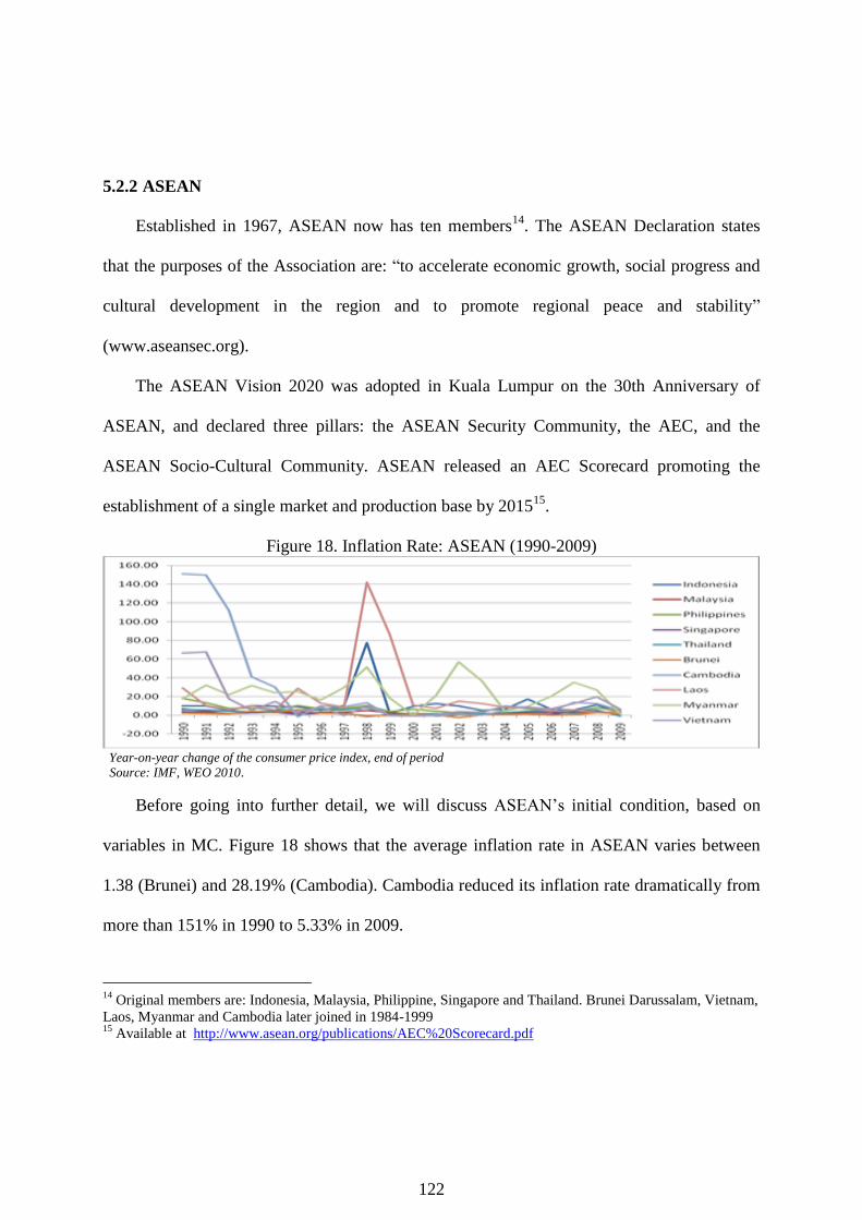
122

5.2.2 ASEAN

Established in 1967, ASEAN now has ten members14

. The ASEAN Declaration states

that the purposes of the Association are: ―to accelerate economic growth, social progress and

cultural development in the region and to promote regional peace and stability‖

(www.aseansec.org).

The ASEAN Vision 2020 was adopted in Kuala Lumpur on the 30th Anniversary of

ASEAN, and declared three pillars: the ASEAN Security Community, the AEC, and the

ASEAN Socio-Cultural Community. ASEAN released an AEC Scorecard promoting the

establishment of a single market and production base by 201515

.

Figure 18. Inflation Rate: ASEAN (1990-2009)

Year-on-year change of the consumer price index, end of period

Source: IMF, WEO 2010.

Before going into further detail, we will discuss ASEAN‘s initial condition, based on

variables in MC. Figure 18 shows that the average inflation rate in ASEAN varies between

1.38 (Brunei) and 28.19% (Cambodia). Cambodia reduced its inflation rate dramatically from

more than 151% in 1990 to 5.33% in 2009.

14

Original members are: Indonesia, Malaysia, Philippine, Singapore and Thailand. Brunei Darussalam, Vietnam,

Laos, Myanmar and Cambodia later joined in 1984-1999 15

Available at http://www.asean.org/publications/AEC%20Scorecard.pdf

http://www.asean.org/publications/AEC%20Scorecard.pdf

123

Figure 19. Interest Rates: ASEAN (1990-2009)

Deposit Interest Rate (%)

Source: World Bank, WDI

Figure 19 shows that Singapore (1.87%) and Cambodia (4.02%) have the lowest interest

rates, while Indonesia (15.41%) and Myanmar (10.46%) have the highest.

Figure 20. Nominal Exchange Rate: ASEAN (1990-2009)

LCU per US$, period average

Source: WDI 2010.

After the Asian economic crisis, ASEAN‘s average exchange rate depreciated sharply,

from 1998 to 2009, it dropped to3753.6. Vietnam (15,330.4) and Brunei (1.64) were the

highest and lowest, respectively. ASEAN countries experienced sharp depreciation in the

exchange rate in 1997-1998.

124

Figure 21. Deficit-to-GDP Ratio: ASEAN (1990-2009)

General Government net lending/borrowing as percent of gross domestic product

Resource: IMF, WEO 2010

In 1990-2009, Singapore experienced an average budget surplus of 9.3%, while Laos (-

5.84%) had the highest budget deficit. In 1990-1997 ASEAN‘s average deficit was -0.55,

lower than 1998-2009, when the deficit averaged -0.94. Laos had the highest deficit in both

periods (-7.52 and -4.72), while Singapore was the lowest (14.78) in the first period, Brunei

(6.11) second.

Figure 22 shows Laos and Vietnam (125.42% and 106.3%) have the highest public debt-

to-GDP ratio, but they both reduced their debts 62.09%, and 50.83% respectively in 2009.

Figure 22. Public Debt-to-GDP Ratio: ASEAN (1990-2009)

General government gross debt as percentage of gross domestic product

Source: WEO 2010.

125

In 1998-2009, the average public debt among ASEAN countries was 57.90, whereas in

1990-1997, this number grew to 77.84. Vietnam (194.75%) had highest public debt in 1990-

1997, Laos (107.48) in 1998-2009. Brunei (-8.97 and 6.80) had the lowest in both periods.

5.2.3 Differences in GDP Per Capita and Population

Compared with ASEAN difference, table 10 shows relatively small differences in GDP

per capita among Eurozone countries in 1992, with an average of 19,361. The highest GDP

per capita was Luxembourg (36,308), 4 times more than Portugal (8,735), which was the

lowest.

Table 21. Population and GDP per capita in the Eurozone (1992)

at Current Price, in Euro Currency

Country Population GDP per capita

(million) Nominal Gap

Austria 7.91 21569 2208

Belgium 10.04 20445 1084

Finland 5.04 18495 -866

France 57.37 20898 1537

Germany 80.59 22536 3175

Ireland 3.56 12002 -7359

Italy 56.86 19275 -86

Luxembourg 0.39 36308 16947

Netherlands 15.18 19228 -133

Portugal 9.83 8735 -10626

Spain 39.01 13481 -5880

Eurozone 285.78 19361

Sources: ECB

Contrary to the EMU, the gap of GDP per capita among nations in ASEAN was huge,

as shown in table 21. The average GDP per capita of ASEAN in 2009 was US$13.679.4.

Singapore had the highest (US$49,765.8), followed by Brunei (US$49,266.8). Both have

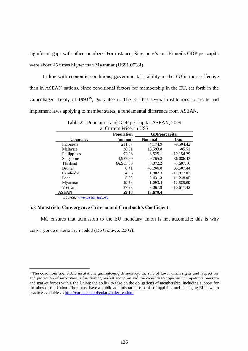
126

significant gaps with other members. For instance, Singapore‘s and Brunei‘s GDP per capita

were about 45 times higher than Myanmar (US$1.093.4).

In line with economic conditions, governmental stability in the EU is more effective

than in ASEAN nations, since conditional factors for membership in the EU, set forth in the

Copenhagen Treaty of 199316

, guarantee it. The EU has several institutions to create and

implement laws applying to member states, a fundamental difference from ASEAN.

Table 22. Population and GDP per capita: ASEAN, 2009

at Current Price, in US$

Countries

Population GDPpercapita

(million) Nominal Gap

Indonesia 231.37 4,174.9 -9,504.42

Malaysia 28.31 13,593.8 -85.51

Philippines 92.23 3,525.1 -10,154.29

Singapore 4,987.60 49,765.8 36,086.43

Thailand 66,903.00 8,072.2 -5,607.16

Brunei 0.41 49,266.8 35,587.44

Cambodia 14.96 1,802.3 -11,877.02

Laos 5.92 2,431.3 -11,248.05

Myanmar 59.53 1,093.4 -12,585.99

Vietnam 87.23 3,067.9 -10,611.42

ASEAN 59.18 13.679.4

Source: www.aseansec.org

5.3 Maastricht Convergence Criteria and Cronbach’s Coefficient

MC ensures that admission to the EU monetary union is not automatic; this is why

convergence criteria are needed (De Grauwe, 2005):

16

The conditions are: stable institutions guaranteeing democracy, the rule of law, human rights and respect for

and protection of minorities; a functioning market economy and the capacity to cope with competitive pressure

and market forces within the Union; the ability to take on the obligations of membership, including support for

the aims of the Union. They must have a public administration capable of applying and managing EU laws in

practice available at: http://europa.eu/pol/enlarg/index_en.htm


http://europa.eu/pol/enlarg/index_en.htm

127

1. Inflation convergence

Fear of inflationary bias in future monetary unions should be avoided that the EMU would

be inclined to inflation. It was assumed that low inflation convergence in the union would

promote economic growth, and limit the risk of destabilizing social conflicts, by decreasing

economic uncertainty .

2. Interest rate convergence

The justification for interest rate convergence was that extreme differences in the interest

rate before joining could lead to large capital gains and losses at the moment of entry.

Hence, if the exchange rate irrevocably fixed, there is no exchange risk until returns on the

euro and other currencies are equalized. Pursuing this similarity in interest rates was meant

to avoid arbitration in financial markets, especially in the period, when there were many

currencies subject to this rigid exchange rate.

3. Exchange Rate Convergence

Exchange rate convergence was intended to prevent countries from manipulating their

exchange rates to force a more favorable exchange rate, with competitiveness as the motive.

Based on the MT, countries should maintain their exchange rate within the normal band of

fluctuation during the two years preceding their entry into the EMU. The upper limit of the

normal band was 2 x 2.25%, and later became 2 x 1.5%).

4. Government Deficit

High budget deficits lead to the crowding-out effect of private expenditures on

consumption and investment, limiting the long-run possibilities of economic growth.

128

5. Public Debt

High government debt creates incentive for surprise inflation, because a large debt will

create a higher default risk. If a country in this state were allowed into the union, the

pressure for a bailout in the event of a default crisis will increase.

Buiter, Corsetti and Roubini (1993) emphasized that fiscal criteria were required to

prevent free riders and spill-over effects, and to ensure fiscal sustainability. This is effective

because such requirements ensure new member states cannot use inflationary measures to

decrease the real value of their public debt, nor devaluate their currency to boost economic

growth.

De Grauwe (2005) explained that the norms of 3% of GDP and 60% budgetary have

been derived from the well-known formula determining the budget deficit needed to stabilize

the government debt: d=gb; Where b is the (steady state) level at which the government debt

will be stabilized (percentage of GDP); g is the growth rate of nominal GDP; and d is the

government budget deficit (percentage of GDP).

The formula shows that to stabilize the government debt at 60%, budget deficits must be

brought to 3% of GDP, if—and only if—the nominal growth rate of the GDP is 5%

(0.03=0.05 x 0.6). This rule is quite arbitrary. It is unclear why debt should be stabilized at

60%, or why this rule is conditioned on the nominal growth rate of the GDP. Seemingly, the

only reason is that 60% was the average of European countries in 1991 (61.7%).

De Grauwe (1996) criticized the MC. He argued that such criteria are neither necessary

nor sufficient to create a successful monetary union. If economic structures in each member

country are similar, asymmetric shocks will not happen. The requirements for interest rate

129

convergence and no devaluation two years before entry into the union are not effective in

forming a successful monetary union. He suggests shifting from convergence requirements

towards institutional development.

Artus (1993) argued a successful economic union is only possible among countries that

have already converged, and has a negligible effect on the integration and flexibility of labor

markets. Krugman (1992) was concerned that economically stronger countries will be

penalized for success, since a country whose booming economy attracts large voluntary

capital inflows will experience more real appreciation. In this case, fiscal criteria make

somewhat more sense, but the question remains: why is fiscal probity a key issue for a

monetary union?

In an empirical study, Artus (1993) showed that in 1992, of 12 EC countries satisfying

all criteria, only France and Luxembourg and other EC countries that could join only

Switzerland satisfies the criteria. Guldager (1996), dividing the criteria of the MT into

inflation and public debt performance, found that five EU Members17

converged towards the

EMU requirements.

Casario and Dadkhah (1998), employing fuzzy18

analysis, found that inflation

convergence fell from 3.8% in 1992 to 3% in 1993 and rose to 3.5% in 1994. Interest rates

have demonstrated significant convergence. Both of these fiscal criteria show that the EU

faces considerable difficulty. The first six years of the period showed a gradual increase in the

degree of budget deficit convergence, and the EU has experienced the least degree of

17

France, Ireland, Spain, Portugal, and the United Kingdom 18

Fuzzy analysis has the potential to aid economic analysis, yet has found most favor with engineers, who have

applied it to a host of forecasting and control problems.

130

convergence in the debt ratio. Some European countries have shown considerable progress

toward meeting the MC.

Green (1994), applying Cronbach‘s coefficient, showed substantial cohesion in nominal

and real exchange rates in ASEAN, little interest rate convergence, and divergent fiscal

variables in the late 1980s. The increasing cohesion, in general, was clear around the same

time.

Xu, Ward and Gan (2007), generated a SVAR model and Kalman Filter19

, concluding

that Singapore, Thailand, and Malaysia are in a favourable position to form a single currency,

due to convergence in nominal exchange rates, inflation rates, positive correlation in external

shocks, and a high degree of correlation in inflation and growth. Azali (2007), using The

Bound Testing Approach on ASEAN-5, found criteria fulfilled in interest rates, inflation rates,

and debt ratio, but not in exchange rates or budget criteria. The findings showed ASEAN-5

countries had the potential to form a single currency.

5.4 Maastricht Convergence Criteria and Cronbach’s Coefficient

Based on previous data, the primary intention of this paper is to investigate whether the

Eurozone and ASEAN met the MC, and to measurethe relative degrees of convergence.

19

An algorithm for sequentially updating a linear projection for a state-space form. When applied to a model in

state-space form, it produces prediction errors ut and prediction error variances Ft.

131

5.4.1 Maastricht Criteria

The Maastricht Treaty agreed that the transition to the final stage of the monetary union

was conditional on a number of convergence criteria20

. Following Artus (1993), we measure

the countries meeting the criteria as follows:

Table 23. Maastricht Criteria and Benchmark Value

Criteria Benchmark of Meeting the Criteria

1. Inflation rate is not more than 1.5% higher than

the average of the three-lowest inflation rates of

EU members.

The countries having average inflation rate value less than or

equal to average of three lowest inflation countries plus 1.5%

015.0)3

( 321

LLL InfInfInf

2. Long-term interest rate is not more than 2%

higher than the average observed in these three

low-inflation countries.

The countries having average interest rate value less than or

equal to average of interest rate value of three lowest inflation

countries plus 2%. Or

02.0)3

( 321

LILILI IntIntInt

3. Has joined the exchange rate mechanism of the

EMS and has not experienced devaluation

during the two years preceding entrance into the

union.

Not Applicable: Since it became obsolete upon transferring

monetary policy to the ECB in the Eurozone; and No

benchmark for criterion for ASEAN.

4. Government budget deficit is not higher than 3%

of its GDP (if it is, it should be declining toward

to the 3%).

The countries having average government deficit-to-GDP

ratio less than or equal to -3%.

5. Government debt should not exceed 60% of

GDP (if it is, it should declining toward the

referenced value).

The countries having average debt-to-GDP ratio less than or

equal to 60%.

Note: InfL1..L3 were inflation rates in three lowest inflation rate countries, and IntLI…L3 were interest rates in three

lowest inflation rate countries.

For ASEAN, the observation period covers 1990-2009. The Asian Crisis in 1997-1998

created severe problems in almost all criteria; therefore, we divided this timeline into 1990-

1997 and 1998-2009. For the Eurozone, the data cover 1983-1992, the period before

ratification of the MT, and 2002-2009, after the euro was introduced.

20

The Maastricht Treaty available at http://www.eurotreaties.com/maastrichtec.pdf

http://www.eurotreaties.com/maastrichtec.pdf

132

5.4.2 The Cronbach’s Coefficient

Following Green (2004), we used Cronbach‘s coefficient21

to analyse the degrees of

convergence among ASEAN and Eurozone members. The estimation model can be seen in

following specification:

k

i

i

k

i

i

x

x

k

k

1

1

var

)var(

11

tCoefficien sCronbach'

Var refers to sample variance; k for numbers of countries; x is variable in MT. The

coefficient value is close to 1 when individual measures convergence and can have large

negative value when divergent22

(Green, 2004). For purposes of measurement, we have

applied these equations to the same periods for each zone as the previous analysis.

5.4.3 Data Specifications

Inflation, in this analysis, refers to the percentage of change in the consumer price index

at the end of each period. The data for ASEAN were from the World Economic Outlook

(WEO) from the IMF. Due to issues with data availability, estimated data still serve as

proxies for historical series. Eurostat data was used for Eurozone analysis; these figures were

designed for international comparison to assess the inflation criterion.

21

Cronbach‘s coefficient measures how well a set of items (or variables) measures a single one-dimensional

latent construct. When data have a multidimensional structure, Cronbach's alpha will usually be low or less than

0.5 (Carmines and Zeller, 1979) and (Cortina, 1993). Instead of alpha, to avoid confusion with other convergent

terminology in this study, we used Cronbach‘s coefficient. 22

It could be happen if the gap between values is very huge for example the huge difference between nominal

exchange rate of Vietnam and nominal exchange rate of Singapore. Since my analysis was consisting of many

countries, multiple years, and more than two countries, the results most probably will be disappearing.

133

Interest rates for both economic zones were taken from deposit interest rate data from

the World Development Indicator (WDI), defined as the rate paid by commercial or similar

banks for demand, time, or savings deposits. Although using deposit interest rate as the proxy

for long-term interest rate was arbitrary, since the sources of data are same, the comparison

will be more reliable.

Nominal exchange rate variables were derived from the WDI, defined as US$ currency /

local currency unit. This proxy was reliable for analysis, as it was relevant to the MC

exchange rate definition.

Deficit data were taken from the WEO for both ASEAN and the Eurozone, with

government net lending/borrowing (percentage of GDP) calculated as revenue minus total

expenditure. The GDP corresponding to each fiscal year was measured at current price (in

national currency). Public debt data were taken from the WEO and is defined as total gross

debt to GDP. Gross debt consists of all liabilities that require payment, or payments of interest

and/or principal, by the debtor to the creditor in the future.

Most data were derived from the WEO, which is comprised of estamated IMF data. To

some extent, the reliability of data for some ASEAN countries , as well as Myanmar, Laos,

Cambodia, was questionable, as was the deficit and debt data of Greece (Lapavitsas, et.al,

2010), which was known to have manipulated statistics to become a member of the EMU.

Regardless of data quality and completeness, these are the data sets we will use as proxies.

Therefore, results should be taken in the context of the limitations of this analysis. Future

analysis may provide more reliable data.

134

5.5 Main Results and Findings

5.5.1 The Eurozone

MC are preconditions that serve as a screening and commitment mechanism, requiring

governments to show their willingness to follow economic policies that do not cost others.

Meeting these goals shows their strong political commitment to mutually beneficial

agreements. Based on table 24, no countries met all criteria during the period from 1983 to

199223

. This result correlates with the findings of Artus (1993), showing that only France and

Luxembourg passed in 1992. The degree of convergence in MC was high (shown by

Cronbach‘s coefficient, except for government deficit).

Table 24. Measurement Results: Eurozone in 1983-1992

Countries Inflation Interest Exchange Deficit Debt

Austria 2.88 3.54 1.06 -2.32 60.14

Belgium 3.49 5.94 1.06 -9.13 61.62

Finland 5.19 7.71 0.81 1.63 55.41

France 4.40 5.34 1.02 -2.80 57.59

Germany 2.31 5.22 1.06 -1.85 60.57

Ireland 4.65 6.19 0.92 -6.53 68.81

Italy 7.39 8.57 0.74 -11.30 63.17

Luxembourg 4.41 5.86 1.06 2.71 -

Netherlands 1.8 3.64 1.06 -4.57 50.14

Portugal 15.07 18.03 0.72 -5.37 45.09

Spain 7.77 10.33 0.77 -4.17 38.12

Maastricht Criteria 3.83 6.13 <-3% <60%

Cronbach’s Coefficient 0.92 0.84 0.98 0.57 0.90 Source: Author’s calculation

23

Austria and Germany failed the debt criterion. France and Luxemburg didn‘t satisfy inflation criteria. Tthe

Netherlands failed the deficit criterion. Ireland and Italy failed almost all criteria.

135

Imposing the MC after the euro launched indicated strong convergence as shown in table

25. Six countries24

met all criteria. The level of nominal convergence based on the MC is very

high (shown by Cronbach‘s coefficient result—almost above 0.9, except for debt criterion).

Coefficient results showed better convergence than in 1983-1992, except for debt criterion,

where the Eurozone was poisoned by the mortgage crisis.

Table 25. Measurement Results: Eurozone (2002-2009)

Countries Inflation Interest Deficit Debt

Austria 1.82 4.13 -1.86 61.03

Belgium 2.01 4.15 -1.28 92.03

Finland 1.57 4.08 2.75 40.70

France 1.89 4.06 -3.73 65.75

Germany 1.64 3.93 -2.42 39.53

Ireland 2.52 4.30 -1.98 34.93

Italy 2.30 4.33 -3.40 98.32

Luxembourg 2.20 3.73 1.08 8.53

Netherlands 1.92 4.06 -1.37 43.50

Portugal 2.35 4.23 -2.35 67.67

Spain 2.93 4.13 -1.43 37.88

Cyprus 2.46 4.90 -2.54 62.55

Greece 3.22 4.47 -6.37 100.59

Malta 2.45 4.81 -4.48 66.04

Slovakia 4.15 4.85 -3.83 35.58

Slovenia 3.96 5.12 -1.44 26.45

Eurozone 2.09 4.11 -2.66 69.92

Maastricht Criteria 3.18 6.05 -3.00 60.00

Cronbach’s Coefficient

(1983-1992, EMU-11) 0.92 0.84 0.57 0.90

Cronbach’s Coefficient

(EMU-16) 0.94 0.95 0.93 0.85 Source: Author’s calculation

5.5.2 ASEAN

Inflation is the core of the MC, due to its risk in causing asymmetric shock. Table 26

shows that in 1990-1997, average inflation criterion was 4.53% and only Malaysia, Singapore,

24

Finland, Germany, Ireland, Luxemburg, Netherlands, and Spain

136

and Brunei met the target figures. From 1998 to 2009, the average was 2.88% and only

Thailand satisfied the requirements. This result seems to correlate with Cronbach‘s coefficient

data from 1998-2009 (0.60), higher than from 1990-1997 (0.51).

Achieving a long-term interest rate is required to convince skeptical financial markets that

inflation rates will stay low. Interest rate data for ASEAN from 1990-1997 shows that MC for

ASEAN is 6.57%. Singapore, Brunei and Cambodia met it. For 1998-2009, the MC for

ASEAN was 5.51%, and Malaysia and Thailand replaced Brunei. This result is in line with

Cronbach‘s coefficient data, which, from 1998-2009 (0.84), is much higher and indicates

better convergence than the period from 1990-1997 (0.58).

Table 26. Measurement Result: ASEAN (1990-2009) Criteria Period MC Average Countries Satisfying Cronbach’s

Coefficient

Inflation Rate 1990-1997 4.53 15.71 Brunei, Singapore, Malaysia 0.51

1998-2009 2.88 8.75 Brunei, Singapore, Malaysia, Thailand 0.60

Interest Rate 1992-1997 6.57 9.22 Brunei, Singapore, Cambodia 0.58

1998-2009 5.51 6.48 Singapore, Malaysia, Thailand, Cambodia 0.84

Exchange Rate 1990-1997 1542.3 0.58

1998-2009 3753.6 0.44

Budget Deficit 1990-1997 <-3% -0.55 Indonesia, Malaysia, The Philippines,

Singapore, Thailand, Vietnam

0.03

1998-2009 <-3% -0.94 Indonesia, Singapore, Thailand, Brunei,

Cambodia, Myanmar

0.40

Public Debt 1990-1997 <60% 77.84 Indonesia, Malaysia, Philippines, Thailand,

Brunei

0.77

1998-2009 <60% 57.90 Indonesia, Malaysia, Philippines, Thailand,

Brunei, Cambodia, Vietnam

0.50

Source: Author’s calculation,

The exchange rate condition in the MT requires member countries to demonstrate the

ability to keep their exchange rate tied to the future monetary union currency. Table 15 shows

that from 1990-1997, ASEAN countries experienced sharp depreciation in 1997-1998.

Cronbach‘s coefficient in 1998-2009 was 0.44, lower than from 1990-1997, indicating weaker

137

convergence. Exchange rate criterion could not be applied since no benchmark currency was

established.

A high government deficit creates an incentive to spur surprise inflation. If a government

borrows to finance its budget deficit, the debt will increase. If it is unchecked, the budget

deficit will create rapid money growth, and eventually, high inflation. For the purposes of

meeting the MC, the deficit must be lower than -3%. From 1990-1997, Indonesia, Malaysia,

the Philippines, Singapore, Thailand, and Vietnam met the criteria; from 1998-2009, Brunei,

Cambodia, and Myanmar replaced the positions of Malaysia, the Philippines, and Vietnam in

satisfying the criteria. Although Cronbach‘s coefficient in 1998-2009 was weak (0.40), it was

better than in the period from 1990-1997 (0.03).

Criteria for the public debt ratio was created to enhance fiscal discipline, to avoid

inflation being lowered temporarily so deficits can be made ―good‖ in any given year. Table

15 shows that ASEAN performance in 1998-2009 was better than that in 1990-1997, in terms

of average public debt and the number of compliant countries. In 1998-2009 the average

public debt was 57.90 and seven countries met the criteria. However, from 1990-1997, the

average public debt reached 77.84 and only five countries were compliant. Five members met

the public debt criteria in the period from 1990-1997, and only Cambodia and Vietnam

satisfied the requirements from 1998-2009. However, Cronbach‘s coefficient in 1998-2009

(0.50) is lower than 0.70 in 1990-1997, indicating weaker convergence.

Overall in the second period, only Thailand met all criteria. Malaysia, Singapore, Brunei,

and Cambodia would probably pass. Malaysia closed to -3.0 in deficit criterion. Singapore

138

must make a concerted effort to meet debt criterion. Brunei and Cambodia were nearly

satisfied the inflation criterion, but the others were far from passing.

The degree of convergence in the Eurozone indicated by Cronbach‘s coefficient data, is

much higher in all criteria except for interest rates. In this area, we achieved the same result

(0.84). Government deficit data (0.57) is comparable to ASEAN (0.40).

Inflation in the Eurozone (0.92) is much higher than that in ASEAN (0.60), as are

exchange rates (0.98 versus 0.44), and debt (0.90 versus 0.50). The reason we see a higher

degree of convergence in the Eurozone in the descriptive analysis, was relatively close figures

in GDP per capita.

Table 27. Measurement Result: ASEAN Countries (1998-2009)

Countries Inflation Interest Exchange Deficit Debt

Indonesia 13.82 14.66 9,289.38 -0.96 53.77

Malaysia 2.43 3.74 3.71 -3.31 42.67

Philippines 5.62 6.58 48.46 -3.43 58.98

Singapore 1.20 1.21 1.64 5.64 91.86

Thailand 2.73 3.38 39.05 -1.79 48.93

Brunei 0.52 5.59 1.64 6.11 6.80

Cambodia 5.21 3.65 3,971.37 -1.64 35.33

Laos 25.77 8.17 8,844.31 -4.72 107.48

Myanmar 23.48 10.56 6.00 -2.05 85.84

Vietnam 6.75 7.25 15,330.4 -3.22 47.33

Total 8.75 6.48 3,753.60 -0.94 57.90

MC 2.88 5.51 -3.00 60

Cronbach’s Coefficient 0.60 0.84 0.44 0.40 0.50 Source: Author’s calculation

Although De Grauwe (1996), Artus (1993) and Krugman (1992) argued the criteria in

MT are neither necessary nor sufficient to create a successful monetary union, the EMU

experienced a higher degree of nominal convergence, and the euro gained an early reputation

for stability as one of the world‘s anchor currencies.

139

The EMU has some weaknesses when facing crises, especially in terms of asymmetric

problems and business-cycle dependence, but the current crisis shows that countries currently

most deeply are the countries in which failed to meet the MC.

Vines (2011) suggested that low inflation and interest rates led to rapid mobilization of

financial flows across borders and induced a debt crisis. This condition was exacerbated by

the limited power of the ECB to control financial circulation. A monetary union on one hand,

without a fiscal union, required members to fall in line with SGP to reduce asymmetric shock.

Thus, fiscal policy imposed constraints for government activity to neutralize the crisis.

Even considering the limitations of the MC, ASEAN can still take significant lessons

from the guiding forces that allowed the euro to emerge as a strong currency and ensure price

stability in the Eurozone. In terms of convergence, ASEAN conditions in 2009 were not as

favorable for introducing a common currency, but this wasn‘t so different from the EU in

1992.

However, seven years after the MT was signed, 11 countries met the MC and the EMU

was able to expand the number of members. Following in the footsteps of the EMU seemed

difficult, because unlike the EU, , ASEAN has much more diversity in income among

countries, a weaker financial sector, and a lack of political preconditions and constitutions

(Madhur, 2002). However, signers of the ASEAN Concord II have committed to form a

single market or reaching AEC by 2015. Based on empirical results, ASEAN in 1998-2009

was not significantly worse than EU in 1983-1992, as shown by Artus (1993) and Guldager

(1996).

140

In terms of the relevant criteria, the inflation criterion will have to be significantly

adapted if it is benchmarked on the ―three best-performing member states in terms of price

stability or lowest inflation rate.‖ The only potential members are Brunei, Singapore,

Malaysia, and Thailand.

Regarding deficit criteria, since ASEAN members were developing countries with the

potential to grow deficits higher than 5%, if the deficit target of 3% were relaxed to 4%, it

would be more applicable to ASEAN.

For the exchange rate criterion, since the currency gap value vis-à-vis the US dollar was

huge, taking the Singapore dollar as the stable anchor was plausible; however, the band

should be determined cautiously.

The current condition of the EMU gives an optimistic perspective for ASEAN, as shown

in the study of Azali (2007). In early stages, to ensure stability, membership should be limited

as suggested by Green (1994) and Xu, Ward and Gan (2007), particularly based on per-capita

GDP.

Creating a monetary union establishes welfare reduction in Brunei and Singapore, as

they should take into account the average preferences of others. For these reasons, MC could

be useful for ASEAN, since it requires candidates to impose uniformity in inflation, interest

rates, exchange rates, and budgets, which will help member countries when facing

asymmetric shock.

The Eurozone crisis indicated that the countries hit hardest by the current crisis were

those unable to meet MC. Clearly, if allowed into the union, the pressure for a bailout of these

nations in the event of a default crisis will increases.

141

5.6 Conclusion

Several critiques addressed by Krugman (1991) and De Grauwe (1996) argue that the

MC had very little to do with convergence and made little economic sense. Seventeen

countries have joined the EMU, and the level of nominal convergence is very high

(Cronbach‘s coefficient above 0.9). Still, it continues expanding as more countries determine

that the benefits outweigh the costs of membership. Despite some limitations in facing the

current crisis (Darvas, 2010), the euro , has evolved into a strong currency; combined with

price stability in the Eurozone, this shows that the monetary and fiscal stability provided by

the MC was a step in the right direction.

ASEAN has high convergence in term of interest rates, but in all criteria, the level of

convergence was below the Eurozone‘s initial position. Given adapted criteria, when

comparing countries satisfying the MC, we find conditions were not much different in the EU

prior to the signing of the MT. Applying the MC to ASEAN countries shows Thailand

meeting all criteria, and most countries satisfying budget criteria, indicating fiscal

sustainability. Thus, the MC was adaptable to ASEAN, with some reformulation of nominal

value, especially in inflation and interest rate criteria (revising the benchmark to average

value).

Adopting the MC can be useful to impose stable macroeconomic performance, if

ASEAN intents to create a deeper integration through a common currency. Similarity in

variables associated with the MC can help member states enhance flexibility in a crisis,

reduce cross-border contagion, and foster growth by promoting financial system soundness.

These efforts must be guided by a strong supranational institution as a binding decision maker.

142

Although some difficulty arises in implementation due to weaker institutions, because of

huge differences in GDP per capita, financial systems, and degree of market liberalization

(Vanderon, 2005), ASEAN should not begin a deeper regional integration abruptly, as the EU

did in the beginning of first stage of the MT.

At this stage, ASEAN still needs a stronger regional surveillance mechanism and should

develop a trigger to accelerate the formation of a common currency. Implementing AFTA,

accelerating the AEC, and increasing economic openness may be the roads to a common

currency, guided by criteria similar to the MC.

143

Chapter 6 Assessing Determinants on Real Convergence and Growth

6.1 Introduction

ASEAN25

may be starting to resemble the EU26

in creating deeper economic integration.

Some members of the EU—which consists of 17 member countries that comprise what is

otherwise known as ―the Eurozone‖27

—have been implementing a European Monetary Union

(EMU) since 1999, while ASEAN‘s 10 member countries are still in the process of achieving

a full free-trade zone.

To create the EMU, EU members needed to agree to surrender their authority over

monetary policy and tighten their respective fiscal policies. Their agreement, signed in

Maastricht, The Netherlands in 1991, had the primary aim of pushing member countries into

nominal convergence, which would transform gradually into real convergence (Marelly and

Signorelly, 2010).

The treaty consisted of several criteria, popularly called the Maastricht Convergence

Criteria (MC). In line with this criteria, by signing a stability growth pact (SGP)28

, Eurozone

members have agreed to continuously satisfy the MC, following the logic that wherever the

euro is applicable, there had to be consistency of fiscal policy to match the single monetary

policy.

25 The Association of Southeast Asian Nations (ASEAN) consists of 10 members: Brunei, Cambodia,Indonesia, Laos, Malaysia, Myanmar,

Philippines, Singapore, Thailand, and Vietnam. 26 The European Union (EU) consists of 27 members. 27 ―The area‖ refers to the countries that use the euro as a common currency. 28 There is an agreement among the Eurozone countries to ensure the stability of the EMU by stressing the implementation of MC in the Eurozone (http://ec.europa.eu/economy_finance/sgp/index_en.htm).

http://ec.europa.eu/economy_finance/sgp/index_en.htm

144

Instilling deeper economic integration by creating a common currency was a good idea

in terms of protecting the Eurozone from financial crisis and economic global uncertainty, and

increasing its level of convergence; however, the recent financial crisis that hit the Eurozone

in 2007-10 raised questions about the future of the EMU and the effectiveness of the criteria

used to achieve convergence and spur growth.

Benassy-Quere and Boone (2010) point out that low growth in the Eurozone resulted

from a lack of enforcement of MC compliance and misguided oversight. However, Irvin

(2005) stresses that in the 1990s growth in the Eurozone was constrained as member countries

tightened their budgets to meet MC, as a condition of joining the Eurozone.

Hein and Truger (2005) note that an incomplete synchronization of the business cycle

across the Eurozone has also contributed to problems. ASEAN, intending to implement a full

ASEAN economic community (AEC) by 2015—as announced at the Cebu Summit in January

2007 (Shimizu, 2010)—should consider the relevant macroeconomic policy lessons offered

by the Eurozone, including the implementation of the MC there.

Among conditional variables determining convergence, changes in demographic

structure played an important role in productivity and growth, as summarized in Bloom and

Williamson (1998). These researchers proposed three main hypotheses about the impact of

demographic variables on growth.

First were ―population pessimists,‖ who believe that rapid population growth is

deteriorating because it tends to overwhelm, and induces technological progress and capital

accumulation. Their second hypothesis centers on ―population optimists,‖ believing that rapid

population growth allows countries to capture economies of scale and promote technological

145

and institutional innovation. The last group they identified was ―population neutralists,‖ who

believe that changes in fertility and mortality imply very different changes in age distribution.

Members of this group argue that population growth affects economic growth insofar as it

affects the ratio of the working-age population to the dependent population.

In looking at the data, we find that generally, in 1990–2010, the real per-capita GDP and

labor productivity of the Eurozone were US$29,054 and US$68,112, respectively—much

higher than the ASEAN‘s figures of US$1,437 and US$19,957 (as calculated from the Unstat

and Total Economic Database). However, ASEAN‘s real per-capita GDP grew three times

faster (3.54%, compared to the Eurozone‘s 1.2%), and its labor productivity grew twice as

fast (2.85%, compared to 1.35%).

Regarding unemployment rates, ASEAN‘s performance was better, as seen in the data:

during this period it was 5.1% (WDI data), compared to 7.8% in the Eurozone (OECD data).

Low income and productivity growth rates, as well as high levels of unemployment in the

Eurozone compared to ASEAN, raises questions about the effectiveness of macroeconomic

policy in the Eurozone, with respect to real convergence and growth.

The purpose of this study is to comparatively reassess the determinants of

macroeconomic policy and demographic variables on convergence and growth, by comparing

the Eurozone and ASEAN. Based on the data and the recent crisis in the Eurozone—more

than a decade after the release of the Euro—we can evaluate the impact of macroeconomic

policy, the MC, on real convergence and economic performance, by comparing a region that

has implemented these criteria with one that has not.

146

To meet this objective, we use the β convergence approach of Barro and Sala-i-Martin

(1992), Solow (1956), and other researchers to review the determinants of convergence and

economic growth.

The study conducted by Soukiazis and Castro (2005) found that the macroeconomic

policy of the MC has made contributions primarily by its restrictive rules vis-à-vis economic

policy and institutional orientation. Castro (2010) addressed the impact of the MC fiscal

criteria on growth, and found that the MC‘s and SGP‘s fiscal roles did not harm growth.

Lombard (2000) confirmed that the enforcement of MC has impeded reductions in

unemployment. Azali et al. (2007), using an autoregressive distributed lag (ARDL) approach,

shows a long-term relationship between variables in the MC and ASEAN growth. Mahmood

and Sial (2012), also using ARDL approach, showed the importance of monetary and fiscal

policies in determining economic growth.

To strengthen estimated results, we compared productivity and unemployment in these

two economic zones. Difference-in-difference (DID) analysis was used to confirm differences

between the Eurozone and ASEAN in the period after the euro was released. We also used

the decomposition approach.

This study breaks research ground in the literature by comparing growth and

convergence in income, productivity, and unemployment between a developed economic

integration area (the Eurozone) and a developing one (ASEAN). Only Soukiazis and Castro

(2005) have examined such issues, and even then, solely within the EU.

As part of a policy evaluation, the current study also seeks to confirm the benefits of

imposing MC on a region, by comparing a region subject to MC to one that is not. Relative to

147

previous empirical studies, some improvements have been made; besides its use of the well-

known β convergence approach, it also uses the DiD and decomposition approaches. The

results will be beneficial in examining the sustainability of regional integration, based mainly

on the Eurozone experience as an ex ante and ex post lesson.

6.2 Productivity, Unemployment, and Maastricht Variables

Before looking in-depth at convergence, it will be helpful to compare the income,

productivity, and unemployment conditions in the Eurozone and ASEAN regions in the

period from 1990–2010.

Figure 23 reports that productivity, or GDP over labor, in these two regions show

upward trends. In the Eurozone, the initial level in 1990 was US$57,878, growing 31% to

US$75,802 in 2010. In ASEAN, the 1990 figure was US$14,274 and the 2010 figure was

US$25,240—a 77% increase.

Figure 23. Productivity and Unemployment Rate: Eurozone and ASEAN (1990-2010)

Note: EZ: Eurozone; P: productivity; and U: unemployment rate. The left axis indicates labor productivity and the right axis unemployment

rate. Sources: Productivity figures were taken from The Conference Board Total Economy Database™, September 2011, http://www.conference-

board.org/data/economydatabase/, and Eurozone unemployment rate figures are from the OECD Stat online database, while those of

ASEAN are from the World Bank, World Development Indicator (WDI).

0

2

4

6

8

10

10000

20000

30000

40000

50000

60000

70000

80000

19

90

19

91

19

92

19

93

19

94

19

95

19

96

19

97

19

98

19

99

20

00

20

01

20

02

20

03

20

04

20

05

20

06

20

07

20

08

20

09

20

10

US$

ASEAN-P

EZ-P

ASEAN-U

EZ-U

http://www.conference-board.org/data/economydatabase/


148

Concerning the unemployment rate, the Eurozone generally had a higher unemployment

rate (7.79%) compared to ASEAN (5.06%). Unemployment rates nonetheless fluctuated, with

those in the Eurozone reaching their highest points in 1994 and 2010, and those in ASEAN

reaching their highest point during the 1997–98 Asian economic crisis.

Figure 24 presents figures pertaining to growth in productivity and unemployment in

these two regions. The increase of productivity in the Eurozone was more stable than ASEAN.

In the Eurozone, the rate of growth ranges from a high of 2.59% in 1994 to a low of –2.47%

in 2009. The ASEAN trend was more erratic: the top per-capita income growth rate was

9.94% in 1995, decreasing sharply to reach the lowest value just three years later (–5.94%).

Figure 24. Growth of Productivity and Unemployment Rate: Eurozone and ASEAN (1991-

2010)

As also seen in Figure 24, unemployment rates were more erratic in the Eurozone than

in ASEAN. ASEAN experienced its highest rate of unemployment growth (1.48%) in 1999,

in line with drops in per-capita GDP and productivity. In the 1990–2008 period, ASEAN‘s

lowest unemployment rate was in 1996 (–0.82%); the Eurozone suffered from high

unemployment while ASEAN saw relatively low unemployment rates. The Eurozone‘s

-6.00

-4.00

-2.00

0.00

2.00

4.00

6.00

8.00

10.00

Pe

rce

nta

ge ASEAN-P

EZ-P

ASEAN-U

EZ-U

149

highest unemployment rate (1.91%) was seen in 2009, in line with the debt crisis the region

experienced.

Figure 25 describes each Eurozone country‘s productivity. The data suggest a growing

trend of productivity in the Eurozone, with slight declines in the last two years, during the

recession suffered by some Eurozone countries.

Figure 25. Labor Productivity in the Eurozone (1980-2010)

Source: The Conference Board Total Economy Database™, September 2011, http://www.conference-

board.org/data/economydatabase/

During 1980-2010, Luxembourg (104,454) enjoyed the highest labor productivity, while

Slovakia (37,534) had the lowest. Ireland demonstrates the highest productivity growth (83%)

and Italy the lowest (26%). The ASEAN data in Figure 26 suggests that Singapore was by far

the highest productive country in ASEAN. On average, ASEAN labor productivity was

15,512; Singapore had the highest (66,506), and Cambodia the lowest (2,612).

This graph shows a huge gap, especially between Singapore and other member countries,

which reflected wide differences among countries in competitiveness, even with similar, and

competing, natural resource endowments and exports, and low technological capabilities. The

graph shows that Vietnam had the highest growth of productivity, starting with only 1,848.

25,00035,00045,00055,00065,00075,00085,00095,000

105,000115,000125,000

1980

1990

2000

2010



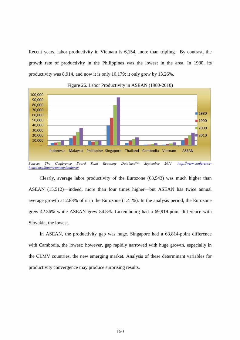
150

Recent years, labor productivity in Vietnam is 6,154, more than tripling. By contrast, the

growth rate of productivity in the Philippines was the lowest in the area. In 1980, its

productivity was 8,914, and now it is only 10,179; it only grew by 13.26%.

Figure 26. Labor Productivity in ASEAN (1980-2010)

Source: The Conference Board Total Economy Database™, September 2011, http://www.conference-

board.org/data/economydatabase/

Clearly, average labor productivity of the Eurozone (63,543) was much higher than

ASEAN (15,512)—indeed, more than four times higher—but ASEAN has twice annual

average growth at 2.83% of it in the Eurozone (1.41%). In the analysis period, the Eurozone

grew 42.36% while ASEAN grew 84.8%. Luxembourg had a 69,919-point difference with

Slovakia, the lowest.

In ASEAN, the productivity gap was huge. Singapore had a 63,814-point difference

with Cambodia, the lowest; however, gap rapidly narrowed with huge growth, especially in

the CLMV countries, the new emerging market. Analysis of these determinant variables for

productivity convergence may produce surprising results.

-

10,000

20,000

30,000

40,000

50,000

60,000

70,000

80,000

90,000

100,000

Indonesia Malaysia Philippine Singapore Thailand Cambodia Vietnam ASEAN

1980

1990

2000

2010



151

Unemployment disparities are often perceived as constant, caused by stable equilibrium

differentials among regional unemployment rates. Labor market adjust toward equilibrium in

the long-run; the convergence of regional unemployment rates was a stabilizer stabilized as

unemployed workers took jobs in other areas, or as capital was infused into a low-wage

region to take advantage of lower labor costs (Blanchard and Katz, 1992). However, if the

speed of adjustment was slow, unemployment disparities might arise as a result of negative

demand shocks, which affect some regions more than others.

Figure 27. Unemployment Rate in the Eurozone (1991-2010)

Source: OECD Stat online database

As seen in Figure 27, the initial Eurozone unemployment rate was 6.20%, with Spain as

the highest (16.24%). On average, Spain has the highest unemployment rate (15.75%) and

Luxembourg the lowest (3.4%); the Eurozone average was 7.9%. This is in line with the

findings of Ljungqvist and Sargent (2008), indicating that in Europe, after the 1970s,

unemployment became persistently higher. Unemployment in Spain and Ireland declined

rapidly at the end of the 1990s, but increased when the crisis hit. Spain reached peaks in its

unemployment rate in 2010 and the early 1990s, both times above 20%.

0.00

5.00

10.00

15.00

20.00

Pe

rce

nta

ge

1990 2000 2010

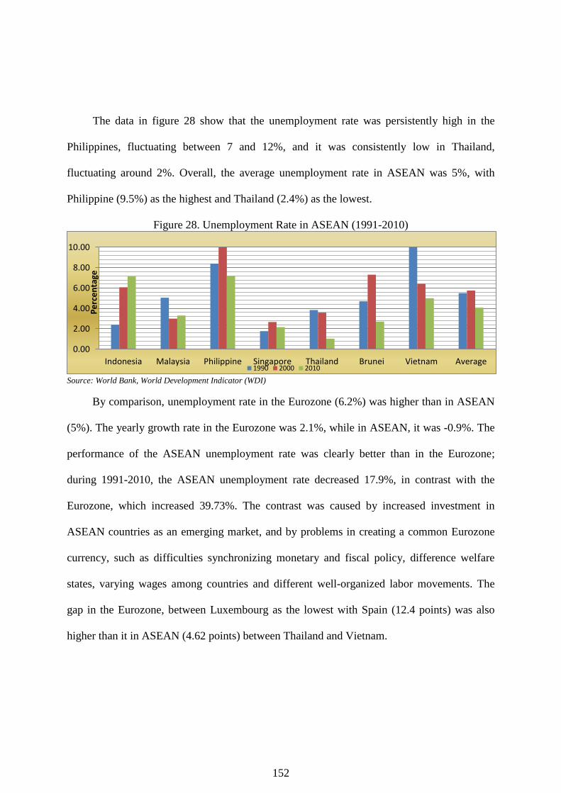
152

The data in figure 28 show that the unemployment rate was persistently high in the

Philippines, fluctuating between 7 and 12%, and it was consistently low in Thailand,

fluctuating around 2%. Overall, the average unemployment rate in ASEAN was 5%, with

Philippine (9.5%) as the highest and Thailand (2.4%) as the lowest.

Figure 28. Unemployment Rate in ASEAN (1991-2010)

Source: World Bank, World Development Indicator (WDI)

By comparison, unemployment rate in the Eurozone (6.2%) was higher than in ASEAN

(5%). The yearly growth rate in the Eurozone was 2.1%, while in ASEAN, it was -0.9%. The

performance of the ASEAN unemployment rate was clearly better than in the Eurozone;

during 1991-2010, the ASEAN unemployment rate decreased 17.9%, in contrast with the

Eurozone, which increased 39.73%. The contrast was caused by increased investment in

ASEAN countries as an emerging market, and by problems in creating a common Eurozone

currency, such as difficulties synchronizing monetary and fiscal policy, difference welfare

states, varying wages among countries and different well-organized labor movements. The

gap in the Eurozone, between Luxembourg as the lowest with Spain (12.4 points) was also

higher than it in ASEAN (4.62 points) between Thailand and Vietnam.

0.00

2.00

4.00

6.00

8.00

10.00

Indonesia Malaysia Philippine Singapore Thailand Brunei Vietnam Average

Pe

rce

nta

ge

1990 2000 2010

153

In January 2002, the Euro was released. The MC became fundamental in ensuring the

stability of this new currency in the region, which meant that compliance among member

countries was essential. In assessing member countries‘ MC compliance, we sought to

measure the current conditions of the Eurozone based on MC requirements. Averaged data

from 2002–10, seen in Table 28, paints a picture of the initial status of each potential member

prior to unification.

Table 28. MC in the Eurozone (2002–10)


Austria 1.85 4.03 –2.38 61.54

Belgium 2.04 4.05 –1.62 92.50

Cyprus 2.68 4.87 –2.86 62.54

Finland 1.43 3.97 2.05 37.82

France 1.72 3.96 –4.12 54.88

Germany 1.51 3.80 –2.51 40.59

Greece 3.31 4.99 –7.97 114.78

Ireland 2.24 4.49 –5.30 31.05

Italy 2.10 4.30 –3.53 99.69

Luxembourg 2.21 3.65 0.76 4.30

Malta 2.35 4.79 –4.47 65.81

Netherlands 1.78 3.94 –1.86 44.39

Portugal 2.24 4.36 –3.32 68.01

Slovakia 4.06 4.74 –4.34 33.12

Slovenia 3.73 4.93 –1.86 27.64

Spain 2.71 4.14 –2.30 39.41

Eurozone 2.37 4.31 –2.85 54.88

MC 3.05 5.90 –3.00 60.00 Source: Author’s calculations

Judging on the inflation criterion, only Slovakia and Slovenia were unable to satisfy the

MC; their inclusion in the zone occurred quite late. In terms of the interest-rate criterion, all

members satisfied it. With respect to fiscal policy, in looking at the deficit criterion, France,

Greece, Ireland, Italy, Malta, Portugal, and Slovakia failed to comply. When evaluating debt,

Belgium, Cyprus, Greece, Italy, Malta, and Portugal satisfied the arbitrary ―60% debt-over-

GDP ratio‖ criterion.

154

Despite the fact that some members were unsuccessful in satisfying various MC, on

average, the Eurozone as a whole satisfied all requirements. However, when looking at the

causes of the most recent crisis in Europe, it is clear that noncompliance with the MC—

especially fiscal criteria—has played a part. For instance, this may explain why Greece had so

much difficulty recovering from the current crisis.

Based on descriptive data, the Eurozone is more stable than ASEAN in terms of

productivity growth, but the former showed more volatile unemployment rates. When

evaluating for MC compliance, almost all members fulfill the monetary criteria, but many

members have been unable to satisfy the fiscal criteria.

6.3 Descriptive DiD and Decomposition

To strengthen the econometric results and best depict income, productivity, and

employment, we employed DiD analysis to determine the impact of deeper regional

integration (i.e. through the introduction of the euro) on productivity and unemployment

growth.

The outcome can be calculated by computing a double difference: one over time (before

and after) and one across subjects (between beneficiaries and non-beneficiaries). This method

is more feasible than any based on a single difference (either over time or between groups),

since examining differences only between beneficiaries and non-beneficiaries will not reveal

the effects of intervention as readily as examining differences in one group across time.

Based on the approach used by Baskaran (2009), we have analyzed the impact of the

release of the euro; however, we have analyzed the period before and after the release, with

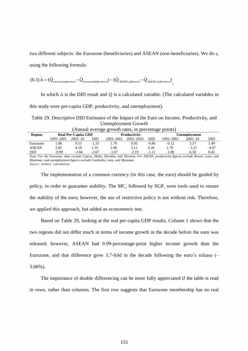
155

two different subjects: the Eurozone (beneficiaries) and ASEAN (non-beneficiaries). We do s,

using the following formula:

)()()1.6(,

_

,

_

,

_

,

_

beforeeuroASEANaftereuroASEANbeforeeuroeurozoneaftereuroeurozoneQQQQ

,

In which is the DID result and Q is a calculated variable. (The calculated variables in

this study were per-capita GDP, productivity, and unemployment).

Table 29. Descriptive DID Estimates of the Impact of the Euro on Income, Productivity, and

Unemployment Growth

(Annual average growth rates, in percentage points) Region Real Per-Capita GDP Productivity Unemployment

1993–2001 2002–10 DID 1993–2001 2002–2010 DID 1993–2001 2002–10 DID

Eurozone 1.86 0.53 –1.33 1.79 0.93 –0.86 –0.12 3.37 3.49

ASEAN 2.85 4.19 1.35 2.86 3.11 0.26 1.76 –3.21 –4.97

DID –0.99 –3.66 –2.67 –1.07 –2.19 –1.11 –1.88 6.58 8.45 Note: For the Eurozone, data exclude Cyprus, Malta, Slovakia, and Slovenia. For ASEAN, productivity figures exclude Brunei, Laos, and

Myanmar, and unemployment figures exclude Cambodia, Laos, and Myanmar.

Source: Authors’ calculations.

The implementation of a common currency (in this case, the euro) should be guided by

policy, in order to guarantee stability. The MC, followed by SGP, were tools used to ensure

the stability of the euro; however, the use of restrictive policy is not without risk. Therefore,

we applied this approach, but added an econometric test.

Based on Table 29, looking at the real per-capita GDP results, Column 1 shows that the

two regions did not differ much in terms of income growth in the decade before the euro was

released; however, ASEAN had 0.99-percentage-point higher income growth than the

Eurozone, and that difference grew 3.7-fold in the decade following the euro‘s release (–

3.66%).

The importance of double differencing can be more fully appreciated if the table is read

in rows, rather than columns. The first row suggests that Eurozone membership has no real

156

benefit: the average income growth in the Eurozone decreased –1.33 percentage points, while

that of ASEAN countries increased by 1.35 percentage points. This results in an overall

difference between the two regions of –2.67 percentage points.

One explanation is that delivering monetary policy to the European Central Bank (ECB),

and tightening fiscal policy, made it difficult for each Eurozone member to avoid the crisis

and induce growth. Fiscal federalism does not allow for addressing regional and structural

asymmetries as stressed in the SGP; therefore, income growth slowed.

ASEAN policy is often used to encourage a free-trade area. One example is the ASEAN

Concord II in 2003, with its goal of forming a single market. Additionally, ASEAN has, in

total, a 2.67-percentage-point higher growth rate than the Eurozone, as a result of not

implementing a common currency—an act that comes with the consequence of policy

constraints.

In the area of productivity growth, Column 2 in Table 29 shows a significant difference

between the two regions in the decade before the euro was released (–1.07 percentage points);

that gap doubled in size in the decade after its release (–2.19 percentage points). If the table is

read by rows, the first row suggests that the release of the euro was relatively ineffective in

promoting productivity: there was a 0.86-percentage-point decrease in the Eurozone, while

ASEAN productivity increased by 0.26 percentage points during that time.

The annual productivity growth in the Eurozone-12 has not successfully increased since

the release of the euro. During the period from 2002-10, it was clear that the countries joining

the Eurozone were significantly less economically successful than the ASEAN countries,

which did not share a common currency—the two areas showed opposing trends. The DID

157

rating is 1.11, showing that ASEAN—which none of the economic policy restrictions that

come with a common currency—performed better in all periods, with a growth rate 1.11-

percentage points higher.

Unemployment conditions are reported in Table 29. Before the release of the euro, the

Eurozone had negative unemployment growth (–0.12 percentage points), higher than ASEAN

(–1.76 percentage points). Later, the opposite condition occurred: the Eurozone suffered from

high growth in unemployment rates and ASEAN experienced large unemployment rate

reductions.

Examining this table by row, we see that the introduction of the euro was painful for the

Eurozone, as economic performance vis-à-vis unemployment worsened (i.e., increasing 3.49

percentage points). The ―big picture‖ of the Eurozone was considerably worse than that of

ASEAN, whose members did not share a common currency. ASEAN performed very well,

with a negative unemployment growth of 3.21 percentage points—quite different from the

4.97 percentage points of the previous period. The overall difference was 8.45 percentage

points, indicating that ASEAN‘s unemployment performance was much better than the

Eurozone.

To acquire a comprehensive understanding of the variables investigated, we use the

same decomposition approach as Bloom et al. (2010) to determine the link between per-capita

GDP (Y/N) and demographic factors:

P

WA

WA

L

L

Y

P

Y

158

In this identity equation, WA represents the working-age population. The identity states

that the level of income per capita equals the level of income per worker times the labor

participation rate (L/WA) times the ratio of working-age to total population (WA/N).

Defining:

So the identity could be:

Totally differentiating the identity, we see that the growth rate of income per capita

equals the growth of income per worker plus the growth of labor participation plus the growth

of the ratio of working-age to total population. That is:

Or

Based on equation (6.2), we divided the analysis into two periods (i.e., 1993–2001 and

2002–09) and compared the Eurozone and ASEAN.

Table 30. Real Per-Capita GDP Decomposition

(Annual average growth rates, in percentage points)

Eurozone ASEAN

1993–2001 2002–09 1993–2001 2002–09

Real per-Capita GDP 2.27 1.19 3.36 3.19

Decomposition

Labor Productivity 1.79 0.78 2.86 2.61

Participation Rate 0.36 0.36 –0.08 –0.04

Working Age to Population 0.13 0.04 0.58 0.62 Note: Authors’ calculations and annual average growth rates in percentage points.

)ln(),ln(),ln(),ln(P

WAwa

WA

Lpr

L

Ylp

P

Yy

waprlpy lnlnlnln

waprlpy lnlnlnln

waprlpy gggg )2.6(

159

Table 30 reports that income growth in ASEAN, as supported in the descriptive and

DID analyses, was higher than that in the Eurozone in all periods. In the first period, the

income growth in ASEAN was higher, supported mainly by productivity. The participation

rate in the labor force declined slightly, since a few subsets of the working-age population

chose education over industry.29

Working age contributed positively, since high population

growth, a result of ASEAN‘s high birth rate in the early 1980s, had translated into a larger

working-age population.

In the second period, income growth in ASEAN decreased slightly due to lower

productivity growth, but it was still higher than the Eurozone. The participation rate improved

by 0.04 percentage points, the same amount as the working-age population.

The growth of per-capita GDP in the Eurozone was also supported by productivity

growth; when productivity growth dropped sharply (by more than half) in the second period,

per-capita GDP also decreased. The participation rate did not change in either period, but the

number of working-age people decreased 0.09 percentage points, contributing to lower

income growth. These results underscore the important contribution of productivity to per-

capita income, as discussed by Bloom et al. (2010).

The decreasing trend in the ASEAN participation rate suggests the development of

middle and higher-level education systems in ASEAN is pushing working-age people to

continue education, rather than joining the workforce. Since the Eurozone faces the long-term

problem of an aging population, the contribution of the working-age population was close to

zero, especially after the 1990s. It will be difficult for any country in this position to support

29

In some cases—for example, Indonesia—policies require individuals to complete a minimum of nine years of schooling.

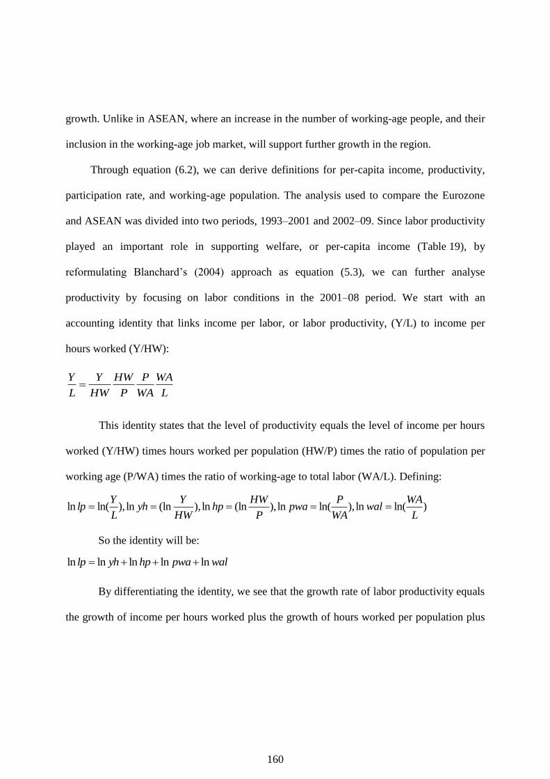
160

growth. Unlike in ASEAN, where an increase in the number of working-age people, and their

inclusion in the working-age job market, will support further growth in the region.

Through equation (6.2), we can derive definitions for per-capita income, productivity,

participation rate, and working-age population. The analysis used to compare the Eurozone

and ASEAN was divided into two periods, 1993–2001 and 2002–09. Since labor productivity

played an important role in supporting welfare, or per-capita income (Table 19), by

reformulating Blanchard‘s (2004) approach as equation (5.3), we can further analyse

productivity by focusing on labor conditions in the 2001–08 period. We start with an

accounting identity that links income per labor, or labor productivity, (Y/L) to income per

hours worked (Y/HW):

This identity states that the level of productivity equals the level of income per hours

worked (Y/HW) times hours worked per population (HW/P) times the ratio of population per

working age (P/WA) times the ratio of working-age to total labor (WA/L). Defining:

So the identity will be:

By differentiating the identity, we see that the growth rate of labor productivity equals

the growth of income per hours worked plus the growth of hours worked per population plus

L

WA

WA

P

P

HW

HW

Y

L

Y

walpwahpyhlp lnlnlnlnln

)ln(ln),ln(ln),(lnln),(lnln),ln(lnL

WAwal

WA

Ppwa

P

HWhp

HW

Yyh

L

Ylp

161

the growth of the ratio of population to working-age and plus working age to total labor. That

is:

Or

Table 31. Productivity Decomposition: 2001–08

(Annual average growth rates, in percentage points)

Eurozone* ASEAN**

Labor Productivity 1.39 5.88

Decomposition

GDP per Hours Worked 1.64 4.11

Hours Worked per Population 0.51 0.47

Population Divided by Working Age –0.02 1.13

Working Age Divided by Labor –0.75 0.16 Note: *Refers to all members of the Eurozone except Malta; **refers to Indonesia, Malaysia, Philippines, and Singapore, due to data limitations.

Looking at the first row, during 2001–08, both regions saw an increase in labor

productivity. The ratio of working-age growth over labor was growing positively in ASEAN,

but it was negative in the Eurozone. The difference could derive from the fact that many

working-age ASEAN people chose to pursue educational opportunities rather than entering

the labor market, the opposite scenario from the aging Eurozone.

Population divided by working age also grew negatively in the Eurozone, but it was

positive in ASEAN, due to a falling mortality rate. In terms of hours worked per population,

ASEAN experienced lower growth. To some extent, this was caused by higher population

growth in ASEAN, as explained previously.

Finally, the increase in labor productivity almost completely accounted for the increase

in GDP per hours worked. We can infer that ASEAN workers enjoyed a very high wage

walpwahpyhlp ggggg )3.6(

walpwahpyhlp lnlnlnlnln

162

increase (4.11 percentage points) compared to their Eurozone counterparts (1.64 percentage

points).

6.4 Theoretical Framework, Data and Model Specification

6.4.1 Convergence

The main purpose of this study is to investigate real convergence in the Eurozone and

ASEAN, as determined by macroeconomic policy related to MC variables. To achieve this

end, we borrow a popular neoclassical model of economic growth, the Solow model.

The study of β convergence is flourishing, as it derives directly from the different rates

of convergence among various countries in the world, indicating that both poor and rich

countries converge toward a steady state (Barro and Sala-i-Martin, 2004). This approach is

used to predict unconditional and conditional convergence.

Unconditional convergence derives from standard neoclassical growth theory, and

relates to diminishing returns on capital properties (Solow, 1956). It occurs when countries

are similar in every respect—with the exception of initial capital stocks, in which case, poorer

countries will grow more quickly than wealthier ones. All countries are assumed to have

access to identical preferences in technology, population, and investment, but differ in their

initial per-capita incomes, and in the access support used to foster the process and grow more

quickly. Under such conditions, there is no suggestion that policies determine economic

growth.

163

Based on some studies, unconditional convergence exists only when countries have the

same level of economic homogeneity. Following Barro and Sala-i-Martin (1992), the typical

unconditional convergence equation could be:

titititi vyyy ,1,1,, lnlnln)4.6(

where y is the real per-capita GDP, is the constant variable, β is the coefficient

indicating convergence, t indicates the time interval, (t – 1) is the initial of the time interval,

and v indicates the error term. To capture the level of unconditional convergence using the β

convergence term, we test the hypothesis that:

10 tgt yeH

where e is the exponential and g is the growth.

1

1

1

ln)1(ln

lnln

lnlnln

tt

tt

ttt

yy

yy

yyygt

The hypothesis suggests that unconditional convergence holds when the coefficient of

the initial dependent variable is negative and between 0 and –1. If β > 0, then yt will increase

enormously, as if β < –1.

Conditional convergence derives from the new endogenous growth theory, which

stresses the importance of not only physical capital, but also human capital and innovation as

determinants of convergence (Barro and Sala-i-Martin, 2004). Conditional convergence

occurs if we control for the determinant of the steady state by relaxing the assumption of

diminishing returns to reproducible factors such as human and physical capital accumulation.

By relaxing the assumption, the growth becomes endogenous, depending on investment

164

decisions that can be determined by policies and institutions. Conditional convergence (i.e.,

conditional on the steady state) implies that there is a negative partial correlation between the

growth rate and the initial level of per-capita income. In this context, unconditional

convergence is not the rule.

When underlying differences in technological progress and other factors are controlled

in the convergence equation, the initial value of per-capita income is found to be strong and

significantly negative, and the theory predicts faster growth for economies that have not yet

reached their steady-state value. Since determinants of economic growth differ across

countries, Barro and Sala-i-Martin (1992) favor the notion of conditional convergence. The

policy and institutional variables in the conditional convergence equation are used as proxies

for differences in country steady-state per-capita GDP level. The general model for analysis

could be:

tititititi vXyyy ,,1,1,, lnlnln)5.6( .

In terms of equation (6.5), a significantly negative β greater than –1 implies that

convergence holds conditionally when γ ≠ 0. Bassanini and Scarpetta (2001), investigating

OECD countries, summarized a number of studies asserting that the condition factors of

convergence include the accumulation of physical and human capital, research and

development, macroeconomic policy-making, financial development, and international trade.

Barro and Sala-i-Martin (1992) concluded that the benchmark rate of convergence

based on cross-country studies is about 2% per year; however, panel analysis has shown that

the rate of growth was actually higher.

165

A vast number of studies investigate income or productivity convergence in either the

Eurozone or ASEAN. Ismail (2008) found conditional convergence in the ASEAN-5 and

showed that ASEAN had a role in improving its own growth. Chowdhury (2005) found an

absence of convergence in ASEAN in a different study period, which was attributed to

missing trade links—a circumstance not conducive to long-term economic growth, and

perhaps a contributor to weak governance among some ASEAN countries.

Vojinovic and Prochniak (2009) confirm the existence of unconditional convergence in

the EU-10 countries, while Kaitila (2005) found conditional convergence of labor

productivity in the EU-15. The latter‘s finding confirms that higher investment, lower public

consumption, and lower inflation each contribute positively to growth, but deeper European

integration is thought to accelerate growth whenever inflation is not part of the equation.

Kaitila (2005) also found conditional convergence among eight central and eastern

European countries in 1993–2002, and suggested that higher investment and public

consumption supported growth in the area. Bijsterbosch and Kolasa (2010), investigating

productivity convergence in Central and Eastern Europe, pinpoint the existence of

convergence and the impact of foreign direct investment inflows.

6.4.2 Maastricht Criteria

The use of the MC as control variables is based on the policy aim of achieving nominal

then, gradually, real convergence (Marelly and Signorelly, 2010). The Maastricht Treaty,

signed in 1991, contains some criteria from the Optimum Currency Area (OCA) theory.

Mongelli (2005) summarizes the properties of OCA, based on many empirical studies: price

166

and wage flexibility, labor market integration, factor market integration, financial market

integration, the degree of economic openness, the diversification of production and

consumption, similarities in inflation rates, fiscal integration, political integration, and

similarity of shocks.

OCA is defined as the optimal geographic domain of a single currency, or of several

currencies whose exchange rates are irrevocably pegged and might be unified. This definition

is based on the work of Mundell (1961), who first introduced the concept of OCA. The

Maastricht Treaty was signed based on the principles of gradualism and convergence criteria.

The criteria capture some of the OCA properties, although the treaty has placed more

emphasis on macroeconomic convergence criteria. The main reason for this emphasis was to

diminish asymmetric shock and increase similarities in policy responses to shock. De Grauwe

(2009) explains:

Inflation Convergence

Inflation Convergence criteria were included in the treaty based on the fear that a future

monetary union would have an inflationary bias. Before the EU started, candidate member

countries were asked to commit to an inflation rate as low as the member countries with the

lowest rate.

During this process, a temporary increase in unemployment was inevitable (i.e., a

movement along the short-term Philips curve). Self-imposed suffering served as additional

evidence that potential member states were serious about fighting inflation. Once they

achieved low inflation rates, they could be safely granted membership. When a common

167

central bank captures the monetary policy of each member, it should reflect the average

preference of the participating countries.

Interest Rate Convergence

The justification for this criterion is that excessively large differences in interest rates

could lead to large capital gains and losses. Suppose a country wanted to enter the monetary

union, but at the moment of entry, its interest rate was higher than the monetary union zone.

As a result, it would be quite attractive for bondholders to sell low-yield monetary union

bonds and buy high-yield candidate country bonds. Thus, economic agents holding monetary

union bonds would see capital losses, and economic agents holding candidate members‘

bonds would see capital gains; either could create disturbances in national capital markets.

Exchange Rate Convergence

The main motivation for this criterion is to prevent countries from manipulating their

exchange rates to force entry at a more favorable exchange rate (i.e., a depreciated one, which

could increase their competitive position).

Budgetary Convergence

High government debt creates an incentive to engineer surprise inflation. Suppose a

member country has long-term bonds with an interest rate fixed in a previous period, based on

prevailing inflation expectations. If the government were to create unexpectedly higher

inflation rates, the real value of these bonds would erode, and the bondholders would derive

insufficient compensation, because the interest rate on their bonds would not reflect this

inflation upsurge.

168

A monetary union between low- and high-debt countries creates a problem for the low-

debt country. In the union, the low-debt country will be confronted with a partner with a

tendency to push for more inflation. As long as one country has a higher debt-to-GDP ratio, it

will have an incentive to create surprise inflation. As a result, the low-debt country stands to

lose, and force the high debt-to-GDP ratio country to reduce it. Once this is achieved, the

incentive to produce inflation disappears, and the candidate country can be safely allowed into

the union.

Relationship between MC and Growth and Convergence

Soukiazis and Castro (2005) investigated the relationships between MC and the

convergence variables of of income, productivity, employment, investment, and

unemployment in the EU-15; they found that for income, there was no absolute convergence;

reducing the deficit was beneficial to the convergence process; and inflation was significant to

growth. As with income, there was no absolute convergence in productivity in the Eurozone,

but conditional convergence existed when the equation was controlled by MC. Together, the

MC have a significant influence on productivity growth and inflation, the latter the only

variable to have a consistent negative influence on productivity growth. Also, in using the MC

as control variables, they found that the EU‘s unemployment converged both unconditionally

and conditionally.

A budget deficit has a negative influence on unemployment growth, and Afxentiou and

Serletis (2000), using the ordinary least squares (OLS) approach, uncovered the significance

of the MC in promoting economic growth. Papaioannou (2010), investigating the influence of

SGP criteria, found that inflation has a significant negative impact on growth; neither deficit

169

nor debt has any impact. He also found that fulfilling SGP criteria has a positive and

significant effect on unemployment.

Savona and Viviani (2003) suggest that an indifferent budget deficit between current

and investment spending limited growth; that public investment contributed positively; that a

high interest rate slowed economic growth; that openness was good for growth; and that

capital formation benefitted growth.

Baskaran (2009), using the DiD approach, found that joining the EMU had an influence

on GDP growth, but no impact on unemployment. Castro (2010), using a dynamic fixed-

effect panel, found conditional convergence in the EU, and that conversion to the euro was

not harmful to growth. He also found that variations in inflation have an impact on growth,

but only in the long term. Lombard (2000) confirms that the imposition of the MC impedes

reductions in unemployment. Finally, Azali et al. (2007), using the ARDL approach, showed

the long-term relationship between variables in the MC and ASEAN growth. Brauninger and

Pannenberg (2002), estimating the relationship between unemployment and productivity

growth by use of an augmented Solow model, found that an increase in unemployment

reduces the long-term productivity level, if unemployment has an effect on labor efficiency.

Some researchers have also tried to estimate the determinants of unemployment.

Ljungqvist and Sargent (2008), investigating the reason for systematically high

unemployment in Europe, found that Europe has strong employment protection and generous

unemployment insurance provisions. Tyrowicz and Wojcik (2010), using the β convergence

approach, found no unconditional unemployment convergence. They also found rural

locations not to be significant, the youth percentage to be significant, and the percentage of

170

individuals over the age of 50 to contribute negatively. Bassanini and Duval (2006), using

panel equations and investigating some macro-level variable shocks, found a significant

impact on unemployment from total factor productivity shock, as well as the terms of trade

shock, interest rate shock, and labor demand shock .

6.4.3 Relation Demographic Variables with Growth and Unemployment

Demographic change has been relatively neglected in the literature. Changes in

demographic structure of the workforce will lead to changes in aggregate human capital, in

the form of experience. Bloom and Williamson (1998)explained thata rise in working age,

brought about by a decline in the fertility rate, can increase income per capita, because output

per worker remains unchanged, but the number of youth dependents declines.

Bloom and Williamson (1998) summarized three main hypotheses about the impact of

demographic variables on growth. First were ―population pessimists,‖ who believe that rapid

population growth is deteriorating because it tends to overwhelm, and induces technological

progress and capital accumulation, as proposed by Coale and Hover (1958) and Ehrlich

(1968).

Their second hypothesis centers on ―population optimists,‖ as proposed by Boserup

(1981), Kuznets (1967) and Simon (1981), who believe that rapid population growth allows

countries to capture economies of scale and promote technological and institutional

innovation.

The last group they identified was ―population neutralists,‖ who believe that changes in

fertility and mortality imply very different changes in age distribution, as discussed by Kelly

171

and Schmidt (1995). Members of this group argue that population growth affects economic

growth insofar as it affects the ratio of the working-age population to the dependent

population.

Population growth attributable to improvements in longevity among the elderly should

have an immediate negative effect on economic growth, implying more elderly dependents to

support. Population growth attributable to a general decline in mortality has no effect, because

the ratio of the economically active population to dependents stays the same. Population

growth attributable to a rise in fertility should have an immediate negative effect on economic

growth given the presence of more mouths to feed, as should population growth stemming

from a fall in infant mortality. These latter demographic effects will, however, have a delayed

positive impact on economic growth, because the economically active population will boom

two decades later.

Bloom, Canning and Sevila (2001) showed that an increase in the working age can

produce deviation to economic growth; Kogel (2001) found a relationship between total factor

productivity and dependency ratio; Persson (2002) found that the age structure of the entire

population affects output; and Sarel (1995) implied the age structure of the population has a

significant effect on output.

Feyrer (2007) indicated that changes in workforce have a strong and significant impact

on the growth rate of productivity, and dependency ratio has no influence on productivity.

Bloom and Finlay (2009) found significant changes in demographics leading to East Asian

growth and labor force growth has a significant and positive influence on growth, as do

working age population and life expectancy. Bloom, et. al, (2010), investigating the impact of

172

demographic change on growth, found that conditional income convergence existed both in

China and India, where working age has a positive impact on growth and life expectancy.

Brauninger and Pannenberg (2002), estimating the relationship between unemployment

and productivity growth with an augmented Solow model, found that an increase in

unemployment reduces the long-run level of productivity, if unemployment has an effect on

labor efficiency.

Some researchers also tried to estimate the determinants of unemployment. Ljungqvist

and Sargent (2008), investigating the reasons for systematic high unemployment in Europe,

found that Europe has strong employment protections and more generous unemployment

insurance. Biagi and Lucifora (2008), using panel estimation, showed a significant

contribution from the 15-24 age group on unemployment.

Tyrowicz and Wojcik (2010), using the β convergence approach, found no

unconditional unemployment convergence. They also found that rural areas were not

significant, the youth percentage was significant, and the percentage of people over 50

contributed negatively. Bassanini and Duval (2006), using a panel equation to investigate

macro variable shocks, found that total factor productivity shock, terms of trade shock,

interest rate shock, and labor demand shock have a significant impact on unemployment. In a

departure from the existing literature, this study intended to address defects and errors, and

provide a clear empirical answer to whether the MC variables, demographic variables, and

typical Barro variables had affected economic growth in ASEAN and the Eurozone.

173

6.4.4 Data

In this analysis, we employed the data shown in Table 32.

Table 32. Relevant Data and Sources Name Definition Source

Per-capita GDP GDP/population Unstat, National Accounts Main Aggregate

Database

Labor Productivity GDP/person employed, in US$ The Conference Board Total Economy

Database

Unemployment Rate Ratio of unemployed to labor force World Development Indicator (WDI) and

World Bank stats for ASEAN; OECD stats for

the Eurozone

Growth of Capital Growth of gross fixed capital formation Unstat, National Accounts Main Aggregate

Database

Openness Ratio of export + import to GDP Unstat, National Accounts Main Aggregate

Database

Working Age Population aged 15–64, as a percentage of total

population

World Bank, WDI

Government

Expenditure

Ratio of government expenditure/GDP World Bank, WDI

Population Growth Percentage derived from birth rate minus death rate,

divided by population

World Bank, WDI

Inflation Percentage of changing consumer price index (CPI) World Bank, WDI

Interest Rate Long-term interest rate WDI and World Bank stats for ASEAN;

OECD stats for Eurozone

Exchange Rate US$ divided by local currency Unstat, National Accounts Main Aggregate

Database

Deficit Deficit ratio divided by GDP WEO stats for ASEAN; OECD stats for

Eurozone

Public Debt Public-debt ratio divided by GDP WEO stats for ASEAN; and OECD stats for

Eurozone

Dependency Ratio Percentage of population -15 and +64 over working

age population

World Bank, WDI

Density People per sq.km. of land area World Bank, WDI

Urban Percentage of population living in urban areas over

total population

World Bank, WDI

Dummy Membership To capture the effect of membership integration: a

member takes a value of 1; all others take a value of 0

www.ecb.int and www.aseansec.org

Dummy Crisis To capture the effect of a crisis in both areas

6.4.5 Model Specifications

Contrary to the existing literature, this study intends to provide a clear empirical

answer to the question of whether the use of MC variables, demographic variables, and

typical Barro variables affects assessments of economic growth in ASEAN and the Eurozone,

using the empirical models below.

174

Real Per-capita GDP

The initial specifications of the equations are consistent with the standard neoclassical

growth model—including the sole convergence factor and the initial level of per-capita GDP.

The first equation tests the hypothesis of unconditional convergence. The extended model

adds the typical input factors, representing investment, openness, population growth, dummy

membership, and dummy crisis. We also follow Soukiazis and Castro (2005) in augmenting

the MC variables and input variables. For income convergence, the equation for the full

model is:

titititi

titititititititititi

vDebtDefER

IntInfOGWAGKDKDMyyya

,,10,9,8

,7,6,5,4,3,2,11,1,, lnlnln)6.6(

where DM is dummy membership, DK is dummy crisis, GK is growth of capital

formation, GWA is growth of working age, O is openness, Inf is inflation rate, Int is interest

rate, ER is exchange rate, Def is the deficit-to-GDP ratio, and Debt is public debt-to GDP

ratio. The countries included in the equation for the Eurozone were all of its members, and the

same was the case for ASEAN.

We captured the impact of demographic variables instead of policy variables, with the

following formula:

titititi

tititititititititi

vUrbanDensDep

GovOGWAGKDKDMyyyb

,,9,8,7

,6,5,4,3,2,11,1,, lnlnln)6.6(

Productivity Convergence

In this study, output per worker is used as a proxy to measure productivity. The

dependent variable is the growth of productivity in relation to its initial level (the convergence

175

factor). Within the real per-capita GDP convergence equation, we induce the same control

variables. The general form of the equation is:

tititititi

tititititititititi

vDebtDefERInt

InfOGPopGKDKDMpppa

,,10,9,8,7

,6,5,4,3,2,11,1,, lnlnln)7.6(

where p is labor productivity and GPop is population growth. The countries included

in the estimation for the Eurozone were all of its member countries. For ASEAN, due to data

limitations, we included only Cambodia, Indonesia, Malaysia, the Philippines, Singapore,

Thailand, and Vietnam.

We also capture the impact of demographic variables instead of policy variables, by

the following formula:

tititititi

tititititititititi

vUrbanDensDepWA

GovOGPopGKDKDMpppb

,,10,9,8,7

,6,5,4,3,2,11,1,, lnlnln)7.6(

Unemployment Convergence

Although the extensive literature of convergence between countries and regions

focuses mostly on per capita income or their related income and productivity measures, this

focus may be fruitfully extended to other areas in economies as Quah (1996) pointed out.

Therefore, in this research I borrow the techniques from the literature on growth convergence.

Theoretical mechanism of convergence process of unemployment is that labor markets adjust

toward equilibrium in the long run, there is convergence of regional unemployment rates

because unemployed workers take jobs in other areas or because capital flows into low-wage

country to take advantage of lower labor costs (Blanchard and Katz, 1992); However if the

speed of adjustment is slow unemployment disparities may arise during adjustment as a result

176

of negative demand shocks affecting some regions more than others (Amsrong and Taylor,

2000).

Following Soukiazis and Castro (2005) which also augmented some Maastricht

Criteria variables on the model as well as other variables, we apply the convergence approach

to test unemployment convergence in both the Eurozone and ASEAN regions. The dependent

variable is the growth of unemployment in relation to its initial level (the convergence factor).

Within the following per-capita GDP convergence equation, we induce the same control

variable. The equation in its general form could be:

tititititi

tititititititititi

vDebtDefERInt

InfOGPopGKDKDMuuua

,,10,9,8,7

,6,5,4,3,2,11,1,, lnlnln)8.6(

where u is the unemployment rate. The countries included in the equation for the

Eurozone are all of its member countries, while for ASEAN, the countries include Brunei,

Indonesia, Malaysia, the Philippines, Singapore, Thailand, and Vietnam.

To estimate productivity, instead of policy variables, we augmented with demographic

variables by using the following formula:

tititititi

tititititititititi

vUrbanDensDepWA

GovOGPopGKDKDMuuub

,,10,9,8,7

,6,5,4,3,2,11,1,, lnlnln)8.6(

6.5 Results

6.5.1 Income Convergence

Using equation (5.6), in line with the findings of Ismail (2008) and Chowdhury (2005)

with respect to ASEAN, and with those of Vojinovic and Prochniak (2009), Castro (2010),

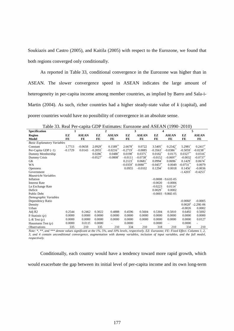
177

Soukiazis and Castro (2005), and Kaitila (2005) with respect to the Eurozone, we found that

both regions converged only conditionally.

As reported in Table 33, conditional convergence in the Eurozone was higher than in

ASEAN. The slower convergence speed in ASEAN indicates the large amount of

heterogeneity in per-capita income among member countries, as implied by Barro and Sala-i-

Martin (2004). As such, richer countries had a higher steady-state value of k (capital), and

poorer countries would have no possibility of convergence in an absolute sense.

Table 33. Real Per-capita GDP Estimates: Eurozone and ASEAN (1990–2010) Specification 1 2 3 4 5

Region EZ ASEAN EZ ASEAN EZ ASEAN EZ ASEAN EZ ASEAN

Model FE FE FE FE FE FE FE FE FE FE

Basic Explanatory Variables

Constant 1.7713 –0.0658 2.0929* 0.1589** 2.6678* 0.0722 3.5405* 0.2542* 5.2981* 0.2417*

Per-Capita GDP (–1) –0.1729 0.0143 –0.2055* –0.0216** –0.2719* –0.0085 –0.3563* –0.0386** -0.5059* -0.0238**

Dummy Membership 0.0286* 0.0480* 0.0198* 0.0375* 0.0182* 0.0175 0.0327** 0.0316* Dummy Crisis –0.0527* –0.0808* –0.0111 –0.0738* –0.0152 –0.0697* -0.0032 -0.0737*

GK 0.2123* 0.0681* 0.0994* 0.0696* 0.1429* 0.0674*

WA –0.0359* 0.0080*** –0.0457* 0.0049 -0.0731** 0.0079 Openness 0.0955 –0.0102 0.1294* 0.0018 0.1456* -0.0036

Government -1.4203* -0.4253*

Maastricht Variables Inflation –0.0008 –9.61E-05

Interest Rate –0.0020 –0.0006

Ln Exchange Rate –0.0223 0.0114* Deficit 0.0029* 0.0002

Public Debt –0.0003 –9.86E-05

Demographic Variables Dependency Ratio -0.0060a -0.0005

Density 0.0020b -2.29E-06

Urban -0.0026 0.0002 Adj R2 0.2544 0.2462 0.3022 0.4888 0.4596 0.5604 0.5304 0.5810 0.6492 0.5692

F-Statistic () 0.0000 0.0000 0.0000 0.0000 0.0000 0.0000 0.0000 0.0000 0.0000 0.0000

L-R Test () 0.0000 0.0000 0.0000 0.0000 0.0000 0.0000 0.0000 0.0000 0.0000 0.0127

Hausmann Test () 0.0000 0.0119 0.0000 – 0.0000 – 0.0000 – 0.0000 -

Observations 335 210 335 210 334 210 318 210 334 210

Note: *, **, and *** denote values significant at the 1%, 5%, and 10% levels, respectively. EZ: Eurozone; FE: Fixed Effect. Columns 1, 2, 3, and 4 contain unconditional convergence, augmentation with dummy variables, inclusion of input variables, and the full model,

respectively.

Conditionally, each country would have a tendency toward more rapid growth, which

would exacerbate the gap between its initial level of per-capita income and its own long-term

178

steady-state per-capita income. Convergence would need to progress considerably to reach a

different steady-state value, especially between old and new members.

Shimizu (2010) shows that some centrifugal forces in intra-ASEAN economic

cooperation—such as an unstable domestic political situation—can also contribute to a slow

convergence speed in the area. The result does not differ markedly from that of Onwuka,

Baharumshah, and Habibullah (2006), who found convergence in ASEAN-5, but not in

ASEAN-10.

The initial release of the euro to initial EU members occurred in 2002, and continued

with each new member until its last release within Slovenia in 2009. Throughout this period,

its was found to have a positive influence on income growth. For its member countries,

joining ASEAN likewise showed consistent positive estimates in all equations.

Both regions suffered from crises—ASEAN in 1998 and the Eurozone in 2009—

although this was found to be insignificant in some equations. When input variables were

inserted into the equation (Column 3), the speed of convergence increased. The Eurozone had

a higher speed (27%) than ASEAN (0.9%).

Individually, growth of capital strongly influenced income growth in both areas and in

all equations, as confirmed by neoclassical theory. Openness correlated positively in the

Eurozone when augmented by the MC, but it was not significant in ASEAN. Increasing the

working age had a negative impact, which confirmed the ―population pessimist‖ view

proposed by Coale and Hover (1958) and in line with Bloom et al. (2010)—tending to

overwhelm and induce a response by technological progress.

179

With respect to the macroeconomic policy variables related to the MC in the Eurozone

only, deficits had an impact on income growth, as indicated by the fact that a one-percentage-

point decrease in deficit pushes growth up by 0.0029 percentage points, as found also by

Soukiazis and Castro (2005).

In ASEAN only, the exchange rate had an influence; a one-percentage-point

depreciation could push growth up by more than 0.01 percentage points. Insignificant public

debt, to some extent, confirmed the finding of Reinhart and Rogoff (2010), who suggested

that the relationship between debt and growth is strong only if debt exceeds 90% in developed

countries or 60% in emerging markets.

On average, the Eurozone countries had achieved nominal convergence (confirmed in

Table 1) and still satisfied the MC and SGP criteria. Although not all MC variables were

significant—also shown by Soukiazis and Castro (2005)—the correlation of all variables was

significant. The result also was in line with Mahmood and Sial (2012), confirming the

importance of monetary and fiscal policy for growth.

6.5.2 Productivity Convergence

Table 34, based on equation (6.7), shows that an unconditional β convergence existed

in the Eurozone, with a convergence rate of 2%, as shown in Column 1; this result aligns with

the findings of Vojinovic and Prochniak (2009).

When augmented with the dummy membership variable, the rate was slower (1.2%),

and joining the economic union had no impact. These findings are in line with Lapavitsas et

al. (2010), who found that Germany enjoys a higher productivity rate, because it has a flexible

180

labor market that attracts cheap labor from countries like Greece, Portugal, Spain, and Italy—

countries with rigid labor markets and strong labor unions.

Table 34. Labor Productivity Estimates: Eurozone and ASEAN (1990–2010)

Specification 1 2 3 4 5


Model RE OLS RE FE RE FE FE FE FE FE

Basic Explanatory Variables

Constant 0.2371* 0.0757** 0.1558* 0.6851* 0.2465* 1.2862* 1.0472* 1.8986* -2.2862 2.6231** Productivity (–1) –0.0201* –0.0048 –0.0125** –0.0743* –0.0214* –0.1385* –0.0930* –0.1972* -0.0630* -0.3314*

Dummy Membership

–0.0029 0.0436** –0.0011 0.0192 0.0009 –0.0273 -0.0005 0.0084**

Dummy Crisis

–0.0364* –0.0891* –0.0248* –0.0687* –0.0348* –0.0525* -0.0341* -0.0548 GK

0.0749* 0.0386* 0.0454* 0.0166 0.0515 0.2881*

GP

–0.0055** –0.0239* –0.0064** –0.0331* -0.0076** -0.0183*

Openness

0.0082* 0.0380** 0.0225* 0.0727* 0.0345* 0.0699* Gov

0.0618 0.0839

Maastricht Variables

Inflation

–0.0026* 0.0005*** Interest Rate

–0.0003 –0.0030*

Ln Exchange Rate

–0.0037 –0.0052

Deficit

–0.0006** 0.0056* Public Debt

–0.0002*** –0.0002

Demographic Variables

Working-Age

0.0335*** 0.0031 Dependency Ratio

0.0132 0.0013

Density

-0.0002** -5.93E-05** Urban

0.0013*** -0.0020

Adj. R-Squared 0.0467 0.0033 0.1873 0.1987 0.3088 0.3004 0.5057 0.4570 0.3192 0.3761

F-Statistic (r) 0.0000 0.2253 0.0000 0.0000 0.0000 0.0000 0.0000 0.0000 0.0000 0.0000 L-R Test (r) 0.0183 0.1883 0.0032 0.0142 0.0003 0.0006 0.0000 0.0000 0.0000 0.0000

Hausmann Test (r) 0.3086 0.038 0.6031 0.0104 0.1425 0.0007 0.0048 - 0.0004 -

Observations 336 147 336 147 334 147 318 147 336 147

Note: *, **, and *** denote values significant at the 1%, 5%, and 10% levels, respectively. EZ: Eurozone; FE: Fixed Effect; RE: Random

Effect; and OLS: Ordinary Least Squares. Columns 1, 2, 3, and 4 contain unconditional convergence, augmentation with dummy

variables, inclusion of input variables, and the full model, respectively.

Incorporating input variables (3), the speed of convergence increased the growth of

capital by 2.1%, and openness encouraged growth. The population took a value of –1, in line

with Coale and Hover (1958). Among macroeconomic policy variables, inflation, as per

Soukiazis and Castro (2005), Papaioannou (2010), and Castro (2010), has an impact on

productivity growth. The result implies that a 1-percentage-point increase in inflation reduces

growth by 0.2 percentage points. A higher debt ratio could restrain productivity growth,

181

although the impact would be relatively small. The impact of the deficit ratio on productivity

growth, in line with the findings of Soukiazis and Castro (2005), was found to be negative.

The speed of convergence increases when we incorporate variables into 9.3% (Column

4). From the result, we determined that macroeconomic policy associated with the MC plays

an important role in determining productivity convergence within a region, given its ability to

explain variations in productivity growth, demonstrated by the adjusted R-squared of 45.7%

and significant joint variables.

The situation with ASEAN is the opposite of the neoclassical assumption: no

unconditional β convergence exists. This result is in line with Chowdhury (2005), and was

significant after incorporating dummy variables.

ASEAN membership had no effect in improving productivity, but the crisis was

significantly painful for members. In applying input variables (Column 3), the speed of

convergence increased, implying that ASEAN conditionally converged at a rate of 13.85%.

The growth of capital formation and openness had positive impacts as a channel for

physical capital and innovation. Population growth had a negative influence, as suggested by

Kelly and Schmidt (1995): the association between population growth and productivity was

negative for the positive effects of scale and induced innovation. Augmentation with policy

variables indicated that inflation, interest rate, and deficit each played a part. A one-

percentage-point increase in inflation promoted productivity by a very small amount, through

the resulting hope of wage increases. The low interest rate served as an incentive for money

circulation to increase by 0.003 percentage points, thus pushing economic activity and

productivity.

182

Comparing all models, we found that policy variables had a great influence in

determining productivity growth, since they had adjusted the R-squared value of 45.7%. The

result was in line with descriptive data showing that the Eurozone had much higher

productivity (US$68,112) than ASEAN (US$29,054). This might be due to a much higher

minimum wage in the Eurozone than in ASEAN, or because the labor–capital ratio is much

higher in ASEAN, reflecting the state of technology there (Blanchard, 2004), attractive to

foreign investment. Although the gap was large (Figure 6), the average growth rate of

productivity in ASEAN (3.5%) was higher than in the Eurozone (1.2%).

Joining the Eurozone had no impact on productivity, but joining ASEAN did have a

positive effect. The inconsequential results of joining the Eurozone are in line with Castro

(2010), who pointed to weak coordination between fiscal and monetary policy, and argued

that there is almost no way of entering a political union that will synchronize fiscal policy,

labor, and the welfare system.

One possible explanation is offered by Ismail (2008): as ASEAN policy improves

openness by implementing AFTA, involving more than 600 million people, it will also

improve the productivity of this emerging market. Therefore, ASEAN has greater potential

for rapid growth than the Eurozone, where the market has already matured.

The impact of economic crisis on productivity was enormous in both areas: the Asian

economic crisis in 1998—as stressed by Mishkin (1999)—was not only economically harmful

but also threw the global financial system into a huge recession. The same was true of the

Eurozone crisis of 2009.

183

These results are consistent with DiD results showing that ASEAN has a higher

productivity growth. A possible explanation is that ASEAN, with its lower capital to labor

ratio, has an incentive for high capital remuneration, and thus, attracts vast capital inflows. As

confirmed by econometric estimations, that physical capital has a significant role in inducing

productivity growth, a complementary factor in the growth of the labor force. This confluence

of circumstances for ASEAN, as an emerging market, has caused an increase in both the rate

of growth and the degree of convergence. On the other hand, the economic role of the euro

has been restrictive, suggesting that stability was causing reductions in the rate of growth.

6.5.3 Unemployment Convergence

Table 35 reports the results for the Eurozone. An unconditional β convergence

(Column 1) exists, since the regression result of initial unemployment did not exceed unity

and was significantly negative. The rate of unconditional convergence was 17.44%, and was

at its highest level when augmented with input variables (12.6%). These results are in line

with the findings of Soukiazis and Castro (2005) and Baskaran (2009).

Eurozone membership has a positive effect on unemployment growth, and the crisis

significantly increased this figure. The growth of investment reduced unemployment. This

finding is in line with neoclassical theory, since it is beneficial for job creation. A one-

percentage-point increase in capital formation can reduce unemployment growth by more than

0.3 percentage points in all equations. Trade openness can also help reduce unemployment,

since a one -percentage-point increase in degree of openness can cause a 0.14-percentage-

point unemployment reduction.

184

The population growth had no significant impact, since it could reflect a general

decline in mortality—as implied by Bloom and Williamson (1998)—and may, therefore, have

no influence. The augmentation of the MC variables into the basic model indicates that

policies adopted to lower the interest rate were responsible for inducing unemployment

growth, and that a deficit reduced it. None of the other variables had a significant role. These

results align with Lombard (2000), who confirms that imposing the MC has impediments that

reduce unemployment. MC variables were explained the fluctuation in unemployment, as the

adjusted-R squared was 50.46%.

Table 35 also reports that ASEAN converged either unconditionally or conditionally,

since the regression result of the previous unemployment rate was negative and does not

exceed unity. This result suggests that the speed of unconditional unemployment convergence

was very high, which is consistent with the homogeneity of unemployment rate among

member countries. When dummy membership was included in the equation, the result

indicated that ASEAN membership had a role in reducing unemployment; ASEAN policies

adopted to induce labor mobility and to increase the degree of cooperation worked to decrease

the unemployment rate.

Economic crisis was insignificant with respect to the growth of unemployment (Figure

24). In times of crisis, ASEAN‘s unemployment rate was relatively stable. This finding

indicates that the Asian crisis in 1998 mainly hit the financial sector and had no real influence

on ASEAN labor, mainly in the agricultural sector.

The highest rates of convergence occurred wherever macroeconomic variables were

inserted into the equation. With the augmentation of input variables, only investment was

185

found to make a significant contribution to reducing the growth of unemployment, since it can

push job creation. The reverse was true in the Eurozone, where openness was not responsible

for fluctuations in the unemployment rate.

Population increases did not contribute to changes in unemployment growth in

ASEAN, as it had in the Eurozone. Among variables related to the MC, we saw that the

exchange rate and public debt each had a significant role in determining unemployment rate.

Single-point currency depreciation was responsible for 0.25 percentage points of

unemployment growth; although the impact was relatively small (0.003), restrictive policy

around public debt has had a positive impact in reducing unemployment.

Table 35 Unemployment Estimates: Eurozone and ASEAN (1991–2010) Specification 1 2 3 4 5


Model RE FE FE FE FE FE FE FE FE FE

Basic Explanatory Variables Constant 0.3544* 0.6030* 0.3047* 0.9028* 0.4250* 1.0302 * 0.3824* –0.1566 12.5030 -2.9600

Unemployment (–

1) –0.1744* –0.4274* –0.1547* –0.4483* –0.1258* –0.4450* –0.1224* –0.5759*

-0.2404* -0.6267* Dummy Membership

0.0039 –0.2820 *** 0.0300*** –0.3512** 0.0427** –0.1161 -0.0007 -0.0884*

Dummy Crisis

0.2106* 0.0828 0.0712** –0.0068 0.0501 –0.0800 0.1335* -0.0501

GK

–0.8063* –0.3754** –0.5164* –0.3200*** -2.4200* -2.2774* GP

–0.0200 –0.0299 0.0018 –0.0154 -0.0145 -0.0674

Openness

–0.1453* 0.012 –0.1489* –0.0026 0.1401** -0.0786 Gov

4.3575* 1.0516


Inflation

–0.0074 –0.0056 Interest Rate

0.0062*** 0.0038

Ln Exchange Rate

0.0161 0.2520*

Deficit

–0.0135* –0.0028

Public Debt

–0.0006 0.0028***


Working-Age

-0.1411 0.0554

Dependency Ratio

-0.0638 -0.0099

Density

-0.0006 0.0008* Urban

0.0029 0.0573*

Adj. R-Squared 0.0896 0.2012 0.1927 0.2108 0.4028 0.2274 0.5046 0.2704 0.3524 0.3228

F-Statistic (r) 0.0001 0.0000 0.0000 0.0000 0.0000 0.0000 0.0000 0.0000 0.0000 0.0000

L-R Test (r) 0.0000 0.0000 0.0327 0.0000 0.0003 0.0001 0.0002 0.0000 0.0000 0.0000

Hausmann Test (r) 0.0000 0.0000 0.0008 0.0000 0.0001 0.0000 0.0000 – 0.0000 - Observations 316 139 316 139 316 139 305 139 330 139

Note: *, **, and *** denote values significant at the 1%, 5%, and 10% levels, respectively. EZ: Eurozone; FE: Fixed Effect; and RE: Random Effect. Columns 1, 2, 3, and 4 contain unconditional convergence, augmentation with dummy variables, inclusion of input

variables, and the full model, respectively.

186

The rate of convergence in ASEAN was higher, both unconditionally and

conditionally. For unconditional convergence, the rates in ASEAN and the Eurozone were

42.7% and 17.4%, respectively. In ASEAN and the Eurozone, the highest rates occurred when

the equation was augmented with policy variables (i.e., 57.6% and 12.2%). Thus, with the

higher rates denoted in Figures 23 and 24 during 1991–2010, the unemployment rate in the

Eurozone was 8%, higher than in ASEAN (5%).

The volatility of unemployment rates also implied that ASEAN was more stable.

Ljungqvist and Sargent (2008) pointed out that after the 1970s, unemployment in the

Eurozone was persistently high, consistent with the generosity of the welfare system. Other

arguments are offered by Lombard (2000) and Bassanini and Duval (2006), who suggested

that the high unemployment rate in the Eurozone was not only the result of generous

unemployment benefits and high minimum wages, but also high hiring and firing costs. Other

perspectives pertain to different wage systems, including the argument that the strength of

labor unions in Europe contributed to a lower degree of unemployment convergence

(Lapavitsas et al., 2010).

ASEAN membership had a negative impact on unemployment, except after being

controlled with MC variables; Eurozone membership, on the other hand, helped explain the

unemployment rate there. The financial crisis was harmful to employment in Eurozone, but

not in ASEAN. In line with this theory, the growth of capital formation was a key factor in

creating job opportunity and lowering the unemployment rate (Soukiazis and Castro, 2005),

as the regression result showed its impact on reductions to unemployment growth in both

areas. For the Eurozone, the growth of capital, openness, the interest rate, and the deficit were

187

determinant variables that explain changes in unemployment growth. For ASEAN, among all

the variables, only the growth of capital, the exchange rate, and public debt influenced

unemployment.

This result aligns with the unemployment DiD result that indicates joining the EU had

no positive impact on unemployment. Again, the restrictive economic policies of the ECB and

the tightening of fiscal policy to stabilize the euro have had a hand in these circumstances.

6.6 Conclusion

This current study addressed the impact of macroeconomic and demographic variables

on growth and convergence in income, productivity, and unemployment in the EU, in the

decade before and the decade after the Euro was introduced.

We presented a comparative study of developed regional integration (i.e., the Eurozone,

which implemented MC) with a developing one (i.e., ASEAN). Data showed that the

Eurozone had a higher per-capita GDP and productivity, but ASEAN performed better in

terms of income growth, productivity growth, and low unemployment levels. Income and

productivity growth were more stable in the Eurozone, but ASEAN had less fluctuation in

unemployment.

Focusing on regression results, convergence was found to be conditional rather than

unconditional, except for the case of unemployment and productivity in the Eurozone. The

ability to explain variation in dependent variables improved substantially when the condition

factor was included as the magnitude of convergence.

Heterogeneity of income and some centrifugal forces in intra-ASEAN economic

cooperation, as noted by Shimizu (2010), also contributed to a slower speed of convergence in

188

ASEAN member countries. A lower capital–labor ratio, combined with higher growth in

productivity, induced a ―catching up‖ process, by which ASEAN derived a comparatively

higher speed of productivity convergence.

Homogeneity in the unemployment rate in ASEAN complemented its different wage

system, and the strength of labor unions in the Eurozone could be a determinant of a faster

speed of unemployment convergence in ASEAN, as also confirmed by Lombard (2000),

Bassanini and Duval (2006), and Lapavitsas et al. (2010).

The augmentation of input variables was essential for all equations. The positive impact

of the growth of fixed capital formation aligned with the neoclassical theory, and the negative

impact of population growth on productivity and working age in per-capita income were in

line with the assertions of Coale and Hoover (1958), indicating that population growth

diminishes growth and induces responses in the form of technological progress and capital

accumulation.

Unfortunately, population growth was found to have no influence on unemployment

volatility. Going deeper into the specific impact of macroeconomic policy (i.e., those relating

to MC) on growth and real convergence, results were mixed in different estimates. In the per-

capita GDP equation, only deficit had a positive influence on growth in the Eurozone, and

depreciation had a positive impact on growth in ASEAN.

The Eurozone‘s productivity estimation results indicated that inflation, deficit, and

public debt had negative effects on productivity growth and on the control of convergence. By

contrast, in ASEAN, inflation and deficit each had a positive impact, and the interest rate

discouraged growth. Looking at unemployment convergence, the interest rate had a positive

189

influence and deficits reduced unemployment. For ASEAN, the exchange rate and debt

contributed positively to unemployment growth.

Due to limitations inherent in the panel estimation, care should be taken with the

interpretation of results, since country-specific effects should differ.Therefore, country-

specific investigations are needed to obtain more robust interpretations. Although individually,

not all variables relating to the MC were significant, in all equations, joint variables were

significant, as indicated by the significance of F-stat results. The results implied that those

macroeconomic policies associated with the MC should not be ignored in promoting

convergence and growth.

Demographic variables were very important relating to productivity in the Eurozone;

however, among included variables, only density had an impact on unemployment. For the

MC variables, the Eurozone‘s policy of keeping inflation low was relevant, since the variable

had the power to reduce productivity and increase unemployment.

For ASEAN, investment was a very important factor for encouraging productivity and

reducing unemployment. Since ASEAN was a new, emerging market, especially after the

CLMV countries joined, providing a good environment was required. For ASEAN, density

had negative impact for productivity and increased unemployment for urban dwellers. In the

case of ASEAN, lower public debt had a negative impact on productivity and increased

unemployment. While the MC as policy variables in both areas appear to play a major role in

shaping productivity and unemployment patterns, demographic conditions are also important.

The result of demographic change in both regions supported the ―population neutralist‖ view

190

that population growth in the short run was not beneficial, but would push the economic

performance in long run.

Economic crisis was painful for both regions, as had been suspected; however, it had no

significance vis-à-vis unemployment. The inclusion of a dummy-membership variable

brought mixed results. It was positive in terms of inducing the growth of per-capita GDP.I It

was beneficial to productivity in ASEAN, but insignificant for the Eurozone. It was beneficial

for reducing ASEAN unemployment growth, but increased the Eurozone‘s figures.

What happened in the Eurozone was implied by Lapavitsas et al. (2011), who asserted

that joining the euro was beneficial for Germany and other core countries, but more peripheral

countries incurred losses when joining the economic union. The data were supported by DID

analysis, the overall results of which showed that ASEAN performed better in terms of

growth of income, productivity, and unemployment.

The comparatively better income performance in ASEAN was supported by higher

productivity and an increased number of working-age people, as shown through

decomposition. The increase in GDP per hours worked—which can be interpreted as wages—

was responsible for the increase in productivity, especially in ASEAN, which experienced

high annual growth.

ASEAN member countries have no macroeconomic policy restrictions, and they

performed better in terms of income, productivity growth, unemployment; however, in term

of the business cycle, the Eurozone was more stable. With respect to this, the main task of the

ECB—as well as the main aim of the MC—is to encourage stability in an area (De Grauwe,

2009), and it was certainly headed in the right direction. The MC could sufficiently push

191

countries to achieve convergence. However, it was difficult to bring about a political union in

the Eurozone, and the region had asymmetrical monetary and fiscal-policy structures.

Therefore, both the MC and the SGP criteria were needed, embedded with incentives to

satisfy member countries, and clear sanctions for non-compliance.

To ensure a stronger euro, a decade after its introduction, some criteria were set forth in

tandem with policy coordination—especially that which imposed price-stability tasks for the

ECB, pushed growth, and mitigated unemployment. ASEAN can learn from the Maastricht

Treaty to implement suitable criteria to increase the likelihood of economic stability and

nominal convergence, if ASEAN intends to adopt a common currency.

Judging the euro as a mistake was premature. We assert, along with Marelly and

Signorelli (2010), that satisfaction of the MC by Eurozone member countries brought about

slow rates of growth as a result of handing over monetary policy to the ECB and tightening

fiscal policy. However, in the long term, those countries will benefit from macroeconomic

stability and convergence.

Research examining the decade before and the decade after the release of the euro

provides us with enough information about real convergence and growth in the Eurozone;

however, future comparative research is still needed to capture more definitive answers.

192

Appendix 6.1

Model Development

The analysis of convergence was based on the neoclassical growth theory framework,

developed mainly by Solow (1956) and Barro and Sala-i-Martin (1992). We start with the

general Cobb–Douglas production function model:

1

,,,, )()1.( titititi LAKYA,

where Yi,t is the total amount of production of the final good at time t in country i, Ki,t is the

capital stock at time t in country i, Ai,t is technology at time t in country i, and Li,t is total

employment in country i at time t. Defining ki,t = Ki,t/Ai,tLi,t as the stock of physical capital per

unit of effective labor, and yi,t = Yi,t/Ai,tLi,t as output per unit of effective labor in country i at

time t, we derive the differential equation:

ititi

t

tikngys

d

dkA )()2.(

.

,

,

where g is the technological progress of A, n is the growth rate of the labor force, and is the

depreciation of K. The production function in the intensive form could be written as yi,t = kα

i,t.

Then, the intensive form of the steady state of capital is:

)ln(1

1ln

1

1ln)3.( *

iiii ngskA

.

Substituting the steady state k* we obtain:

193

)ln(1

ln1

)ln(ln)4.( ,,

*

iiitioii ngsgAyA

.

Following Barro and Martin (1992), the unconditional income convergent equation would be:

titititi vyyyA ,1,1,, lnlnln)5.( ,

where y is real GDP per capita, is the constant variable, β is the coefficient indicating

convergence, t indicates the time interval, (t – 1) is the initial of the time interval, and v

indicates the error term. Since the production function in the intensive form can be written as

yi,t = kα

i,t. substituting the steady state k* in (3), we obtain:

1

*

)()6.(ng

s

AL

YA

i

Taking the log at both sides:

)ln(1

ln1

)ln()7.(

*

iii

i

ngsAL

YA

Defining productivity at the steady state as p* = (Y/L)* then:

1

01* )().()8.(

ng

seA

ng

sApA gt

i

.

Taking the log at both sides:

)ln(1

ln1

ln)9.( 0

*

,

iiiti ngsgtApA

Following Barro and Sala-i-Martin (1992), the unconditional productivity convergent

equation would be:

titit vppA ,1,lnln)10.(

194

Recent literature on economic convergence among countries and regions focuses mostly

on per-capita income or other related productivity measures. Therefore, like Soukiazis and

Castro (2005), we borrowed the convergence approach to test unconditional and conditional

convergence in both the Eurozone and ASEAN. The equation for unconditional

unemployment convergence was:

titit vuuA ,1,lnln)11.( .

Since determinants of economic growth differed across countries, Barro and Sala-i-

Martin (1992) favored the notion of conditional convergence. The policy and institutional

variables in the conditional convergence equation are used as proxies for differences in

country steady-state per-capita GDP. The general model for analysis could be:

.

tititititi vXqqqA ,,1,1,, lnlnln)12.(

195

Chapter 7 Augmented Analysis of Economic Integration Impact on Trade

7.1 Introduction

After previously investigated the level of nominal and real convergence in chapter 5 and

6, according to Linder (1961), the trade will be more intensive in goods that have overlapping

demand. It implies that international trade will be more intense between countries with similar

per capita income levels or have converged. Before the crisis hit the Eurozone in 2007-2009,

creating a common currency was seen as a good way to exploit potential benefit from trade,

and the European Monetary Union (EMU) looked like an ideal model for the emerging

ASEAN economy. The success of the euro‘s launch, its evolution into a strong currency, and

relative price stability in the Eurozone were the signs that the monetary and fiscal stability

provided by the Maastricht Criteria (MC) were steps in the right direction.

According to Mutaqin and Ichihashi (2013), however, many of the Eurozone countries

now suffering most deeply after the economic crisis, are mainly those that violated the

parameters of the Maastricht Treaty and Strong Growth Pact (SGP). Therefore, ASEAN may

not be remiss following in the footsteps of the European Union (EU) to create deeper regional

economic integration.

The main aim of this paper is to comparatively investigate the impact of different levels

of economic integration on bilateral trade in two areas, one region having a common currency

(the Eurozone), and the other a struggling free-trade area (ASEAN).

This paper centers on the following research questions:

196

Whether the different integration process has exerted a different impact on intra original

and original-new bilateral trade relationships;

Whether membership enlargement impact was positive;

Whether convergence in variables associated with the MC were significant; and

Whether new trade theory and H-O hypotheses could explain the phenomena.

To answer these questions, we augment the gravity model by combining the micro

approach with macro approach (MC variables).

Economic integration is often described using the five stages of the Balassa model.

Pelkmans (2001) divides the steps thusly: (1) Free trade area (FTA), (2) Custom union (CU),

(3) Common Market (CM), (4) Economic Union, and (5) Total Economic Integration. Today,

17 of the 27 members of EU form the European Monetary Union (EMU), initiated by 11

members in 1999. According to the Balassa model, this union has advanced past Stage 4 but

hasn‘t reached Stage 5.

ASEAN started with 6 members, growing to 10 after allowing Cambodia, Laos,

Myanmar and Vietnam (CLMC) to become members. They are now in the process of

accomplishing an ASEAN FTA and intend to achieve CM by launching the ASEAN

Economic Community by 2015.

Countries joining a common currency weigh the potential benefit of joining against the

inevitable cost (Mico, Stein and Ordonez, 2003). Benefits like a reduction in transaction cost

when trading goods and services between countries with different currencies will tend to

benefit countries heavily involved in international trade. On the other hand, costs may include

197

the possibility of dampening business cycle fluctuation through independent, counter-cyclic

monetary policy.

The EU designed institutions to assure economic convergence prior to introduction of

the Euro. The Maastricht Criteria (MC), following Maastricht Treaty (MT) in 1991, were

strict guidelines for member states to follow, with the ultimate goal of adopting a single

currency. In order to maximize the benefit and minimize the cost, the MC enforced

convergence in several factors: inflation rate, interest rate, and exchange rate as monetary

criteria; deficit and debt-to-GDP ratio as fiscal criteria (Afxentiou, 2000). Although

conditions in the Eurozone have worsened in terms of income and productivity growth, and

the EU has experienced a high level of unemployment, the significance of the MC in

determining real convergence indicated the criteria were sufficient to achieve convergence

and stability, as shown by Mutaqin and Ichihashi (2012).

To achieve these goals, as stressed by Marelli and Signorelli (2010), member countries

in the short term will suffer from slow growth as a result of surrendering monetary policy to

the ECB and tightening fiscal policy, but in the long run, countries will benefit from

macroeconomic stability, such as price stability, fiscal discipline, removal of exchange rate

risks, reduced uncertainty about inflation and interest rates, and increased investment and

international trade.

The adoption of the common currency in 1999, followed by the release of the euro coin,

concluded the European convergence process. As expected in the process of creating a

common currency, trade barriers between member states in the Eurozone had already been

removed during the 1990s. Sharing a common currency may further deepen real economic

198

integration—directly, through reduced trade costs, and indirectly, through intensified

competition due to enhanced price transparency (Belke and Spies, 2008).

Despite some limitations, seventeen countries have joined the EMU, and it continues

expanding, as more countries decide the benefits outweigh the costs of membership (Darvas,

2010). At the European Council summit in Copenhagen (June 1993), the Union invited the

Central and Eastern European countries (CEEC) to enter the EU with the contingencies that

the nations guarantee democracy, develop market economies, and fulfill membership

obligation30

. Following the Copenhagen Treaty, six countries joined the EU. Greece joined in

2001, followed by Slovenia in 2007, Malta and Cyprus in 2008, Slovakia in 2009, and finally,

Estonia in 2011.

ASEAN also expanded their membership by preparing Indo-Chinese countries to be

members thorough the Treaty of Amity and Cooperation in Southeast Asia in 1976. Although

Vietnam refused the invitation, the resolution of the Cambodia Crisis paved the way for

reconciliation between ASEAN and the Indo-Chinese countries. Finally, the Singapore

declaration in 1992 allowed all Southeast Asian Countries to be members of ASEAN

(Angresano, 2004).

The ASEAN free-trade area (AFTA) was established in 1992, and was one of the most

important regional trade arrangements in Asia, aimed at eliminating tariff barriers among

member countries through agreement on the Common Effective Preferential Tariff (CEPT)

scheme. Eliminating tariffs should induce higher intra-regional trade among ASEAN

30

http://ec.europa.eu/enlargement/enlargement_process/accession_process/criteria/index_en.htm

http://ec.europa.eu/enlargement/enlargement_process/accession_process/criteria/index_en.htm

199

members, and AFTA was expected to become a full free-trade area by the year 2008 (ASEAN

Secretariat).

In mid-1997, the Asian financial crisis suddenly erupted. According to Hill and Menon

(2010), it had serious ramifications for ASEAN. For some time, the region lost some of its

commercial appeal, and ASEAN was seen by many as an ineffective and feeble institution,

unable to respond decisively at a time of crisis. The crisis urged ASEAN to accelerate AFTA

implementation, agreed at the ASEAN summit at Hanoi in 1998. The story of this crisis,

however, played out similarly to the most developed countries situated or in the Eurozone.

A decade after the euro, the crisis erupting in the Eurozone has made the benefits of a

common currency less attractive, especially for trade. Although the situations sound similar,

there are structural differences between the proposed AEC and the European Economic

Community. Most notably, individual ASEAN countries are reluctant to give up nationalistic

economic policies about non-members; the AEC guidelines will not include a common

external tariff. This should not be too surprising, as there are huge discrepancies between the

member states in average external tariff levels (Cuyvers, Lombaerde and Verherstraeten

2005). Thus, the lesson of the EMU will provide insight into the future development of

ASEAN.

The rise in globalization fosters an increasing number of studies on the source of trade.

In reality, the main international trade pattern is multilateral; however, investigation would be

hampered by data limitations and methods. Thus, using the gravity model as a bilateral trade

model emerged as the appropriate method. Used by many researchers, the approach was

clearer, and it was convenient to explain trade patterns. According to Yamarik and Ghosh

200

(2005), the gravity model has become extremely popular in empirical trade literature, for

many reasons, because:

Modern theories of trade, based on differentiated products, provide an improved

theoretical foundation for the equation.

The model has proved quite successful in estimating bilateral flows.

There is an increased interest in empirical testing of the trade effects on regional trading

arrangements.

And, among economists, there has been new interest in the subject of geography and

trade.

Based on Newton‘s law of gravitation, the model predicts that the volume of trade

between two countries should increase with size and decrease with transaction cost (the proxy

was distance).

Helpman (1987) provides the theoretical foundation to build the augmented model,

which is based on a micro foundation approach to new trade theory (size and similarity), and

Heckscher-Ohlin theory (relative factor endowment). Egger and Pfaffermayr (2013) use

Helpman‘s approach to explain the pure effects of European integration, and Warin, Wunnava,

and Janicki (2009) combine Helpman‘s model with convergence measures (MC), to explore

the bilateral FDI of EU countries.

This study is differentiated from previous works in several respects. First, this analysis

provides a better understanding of the impact of different stages of integration on trade.

Second, this study measures the effectiveness of regional economic integration on trade,

especially in the current global crisis. Third, the study combined micro approach variables

201

(size, similarity, and endowment) with macro approach variables (associated with MC).

Fourth, although there are a number of studies on the effects of regional economic integration,

little research has compared the effects of the euro on the Eurozone and AFTA in ASEAN.

Trade Pattern

Figure 29 shows average bilateral intra-Eurozone and intra-ASEAN trade. On average,

bilateral trade in the Eurozone (43.72%) was almost double ASEAN (24.20%). The highest

degree of reciprocity in the Eurozone was in 1992 (46.88%) and in ASEAN was in 2009

(26.32%). Overall, bilateral trade in the Eurozone is declining, while in ASEAN, the trend is

improving. The increasing trend for ASEAN implies that and outward-looking strategy, the

hallmark of ASEAN, encourages high trade volume (Cuyvers, De Lobaerde and

Verherstraeten 2005).

Figure 29. Bilateral Trade over Total Trade: ASEAN and Eurozone (1990-2009)

Author’s calculations, dividing bilateral trade over total trade, in percent.

Source: DOTS, IMF

Further detail for the EU‘s main trading partners is shown in Figure 30, which shows

that domestic destinations (intra-EU) contribute the highest portion by 18.9%. Unfortunately,

0

10

20

30

40

50

19901991199219931994199519961997199819992000200120022003200420052006200720082009

ASEAN Eurozone AV-ASEAN AV-Eurozone

202

the trend was decreasing by -1.2% annually. The USA was the second most important partner

for the EU by 16.98%; however, their share was also declining.

China emerged as the EU‘s most important partner, by 265% from 1993 to 2009. The

emergence of China as a major player in international trade, was due to their rapid economic

growth from investment, a direct result of their open-door policy. As the most highly

populated area in the world, China also has a reputation for its trading commodity

competitiveness.

Figure 30. Percentage Share of EU Trade by Trading Partner (1993-2009)

Source: Eurostat

Japan held the highest share of ASEAN trade in 1993-2009, with 13.4%. However, in

2009, China and the EU took over this position. China-ASEAN trade intensity grew by 465%,

from 2.1% in 1993 to 11.58% in 2009. USA-ASEAN trade narrowed from 17.7% in 1993 to

9.76% in 2009.

Figure 31 shows that ASEAN intra-trade intensity was the higest share of trade by

22.8%, and increasing. The declining influence of the USA in the recent past might be caused

by the recession, as well as loss of competitiveness with commodities traded by China.

0

20

40

60

80

100

1993 1996 2000 2002 2003 2004 2005 2006 2007 2008 2009EU USA China Japan South Korea Russia India Others

203

The degree of bilateral trade intensity among Eurozone countries is shown in Figure 32.

Portugal has the highest degree of dependency with other Eurozone members, with the

highest average degree of trade (62.4%), followed by Austria (61.2%). Ireland has the lowest

trade intensity with other members at only 27.3%, which might be explained by their

geographic position, close relationship with the United Kingdom, and huge investments in

high technology.

Figure 31. Percentage Share of ASEAN Trade by Trading Partner (1993-2009)

Note: Exclude Laos prior to 2003; Vietnam Prior to 2004; and Cambodia and Myanmar prior to 2002.

Source: ASEAN Trade Statistics Database

Among new member states (NMS), Slovenia has the highest trade relationship with

other members, at 59.8%, and Cyprus has the lowest (40.9%). An interesting result was

shown by France, where the degree of trade with other original members only accounts for

70%, very different from other member states. Its relative geographical position might be the

reason for the different level of trade intensity with other member states.

At the country level, Germany, as the biggest country in term of GDP, dominated

bilateral trade with other members within the Eurozone (Appendix 7.1), more than a 10%

portion with all members.

0

20

40

60

80

100

1993 1996 2000 2002 2003 2004 2005 2006 2007 2008 2009ASEAN Australia China EU India Japan USA Others

204

Figure 32. Average Intra-Eurozone Bilateral Trade by percentage (1990-2009)

NMS was: Cyprus, Greece, Malta Slovakia and Slovenia. The ratio may be undervalued due to excluding Belgium and

Luxembourg.

Source: DOTS, IMF, Author’s calculations, dividing bilateral trade by total trade

For ASEAN, Laos was highly interrelated with other ASEAN, with the highest trade

volume, 61.6%, followed by Myanmar (39.9%) and Cambodia (39.6%). The fact that Laos is

a land-locked country might explain why the degree of dependency with neighbor countries

was so high. Within the ASEAN-6, Brunei did the most trading with other ASEAN members

(30.7%), followed by Singapore (25.8%). The Philippines was the country with the lowest

relationship with other ASEAN members (14.5%). Clearly, geographical position plays an

important role in different degrees of trade intensity with neighboring countries. At the

country level, Singapore, which implemented a null tariff, was the primary trading partner for

all ASEAN members, except Laos (for details, please see Appendix 2).

20

30

40

50

60

Eurozone Original

205

Figure 33. Average Intra-ASEAN Bilateral Trade by percentage (1990-2009)

Source: DOTS, IMF

Author’s calculation, dividing bilateral trade by total trade

Generally, trading among neighboring countries made the dominant contribution to total

trade in both the Eurozone and ASEAN. This suggests that creating regional economic

integration might contribute to higher welfare through higher trade intensity. Despite a

critique from Elliott and Ikemoto (2004)—arguing that apparent robust economic

performance from ASEAN countries stems mainly from extra-regional rather than intra-

regional trade—removing trade barriers across borders in ASEAN still played an important

role in developing this huge ASEAN market of more than 500 million people.

To stimulate faster economic cooperation among member countries, ASEAN

established AFTA in 1992, aiming to eliminate tariff barriers among members. The agreement

on the Common Effective Preferential Tariff (CEPT) scheme required that tariffs applied to a

wide range of products traded within the region be reduced to no more than 5%. It applied to

all products from ASEAN member countries, defined as those products made with at least

40% ASEAN content. New ASEAN members, including Cambodia, Laos, Myanmar, and

5

15

25

35

45

55

65

Indonesia Malaysia Philippine Singapore Thailand Brunei Cambodia Laos Myanmark Vietnam

ASEAN ASEAN6

206

Vietnam, have also implemented the CEPT scheme, with 80% of their products included in

the CEPT list (ASEAN Secretariat).

Table 36. Average CEPT Rates, By Country, 1993-2003 Country 1993 1994 1995 1996 1997 1998 1999 2000 2001 2002 2003

Indonesia 17.27 17.27 15.22 10.39 8.53 7.06 5.36 4.76 4.27 3.69 2.17

Malaysia 10.79 10 9.21 4.56 4.12 3.46 3.2 3.32 2.71 2.62 1.95

Philippines 12.45 11.37 10.45 9.55 9.22 7.22 7.34 5.18 4.48 4.13 3.82

Singapore 0 0 0 0 0 0 0 0 0 0 0

Thailand 19.85 19.84 18.16 14.21 12.91 10.24 9.58 6.12 5.67 4.97 4.63

Brunei 3.78 2.64 2.54 2.02 1.61 1.37 1.55 1.26 1.17 0.96 1.04

ASEAN6 11.44 10.97 10 7.15 6.38 5.22 4.79 3.64 3.22 2.89 2.39

Cambodia 10.39 10.39 8.89 7.94

Laos 5 7.54 7.07 7.08 6.72 5.86

Myanmar 2.39 4.45 4.43 4.57 4.72 4.61

Vietnam 0.92 4.59 3.95 7.11 7.25 6.75 6.92 6.43

ASEAN10 7.03 6.32 4.91 5.01 4.43 4.11 3.84 3.33

Source: ASEAN Secretariat

ASEAN is well respected for its rapid economic development over the past 25 years.

AFTA was fostered upon recognition that most of the region‘s trade was extra-regional. The

preferential tariff reduction schedule was ambitious and rapid, so AFTA had to accelerate the

pace of multilateral trade liberalization in ASEAN-6 countries.

7.2 The Significance of Bilateral Trade within Economic Integration

The main benefit of deepening economic integration, primarily through implementing a

common currency, is reducing transaction costs. Regardless of limitations, the optimum

currency area (OCA) theory was a guide to weigh the potential benefit of joining an economic

union against the inevitable cost. Until recently, two main hypotheses come into play

regarding OCA endogeneity. The first, proposed by Frankel and Rose (1996), then adopted by

the ECB, argues that economic integration will affect the symmetry of output fluctuation by

207

removal of trade barriers, raising trade, allowing demand shocks to more easily spread,

leading to more correlated business cycles, and more correlated policy shocks.

Krugman (1981) proposes a different argument suggesting that economic integration leads

to more asymmetric macroeconomic fluctuations through better risk-sharing opportunities,

leading to more attractive specialization in production, and rendering macroeconomic

fluctuations less symmetric.

Based on the seminal paper by Frankel and Rose (1996), the endogeneity of an OCA

became a focus for many economists, with various methods and objects of study. Their

research suggests that closer trade relations result in a convergence of business cycles.

Furthermore, similar business cycles create good preconditions for policy integration and the

creation of a currency area.

Endogeneity of an OCA according to Schiavo (2006), can be defined as a change in the

nature of the shocks faced by member countries, triggered by adoption of a single currency.

Following OCA theory, the EU set up the MC as a policy guide to avoid risks of asymmetric

shock. Further, Warin et.al (2009), using the MC as control variables, suggested that

economic convergence ensured by belonging to the common currency are helps double FDI

flow.

A single medium of exchange should reduce transaction costs and thereby facilitate

international trade (Mundel 1973). Having a common currency eliminates bilateral nominal

exchange rate volatility, and thus reduces the uncertainty and risk involved in trade

transactions. While there are ways to hedge against this risk, doing so may be costly. Kenen

(2003) point out that it is not always possible to fully hedge against large, long-lasting

208

changes in exchange rates, since producers are uncertain not only about the price they will

receive for their exports, but also about the demand for their products. In this case, a producer

does not know how much foreign currency will be earned, and how much should be sold in

the forward market.

Despite this argument‘s intuitive appeal, the evidence regarding the impact of exchange

rate volatility on trade has not yielded a conclusive result. There is some empirical evidence

suggesting that exchange rate volatility has a negative effect, but these effects are generally

quite small, have decreased over time, and vary widely in significance, depending on the

study in question (Sousa, 2012). The effect of joining a currency union eliminates the

transaction costs arising from trading across countries with different currencies, independent

of the volatility channel.

Sharing a common currency has an additional effect: it results in irrevocably fixed

exchange rates, thus eliminating exchange rate volatility between the currency union partners

for the foreseeable future. This may increase market transparency and foster competition

among firms in different countries. Finally, in giving up their national currencies and adopting

a much more liquid currency, the monetary union may also provide its member countries with

a vehicle to hedge exchange rate risk in their trade transactions with non-member countries. In

the EU, the euro increased trade flows not only among members, but also with other trading

partners as well.

Rose (2000) found that a common currency triggers bilateral trade. Glick and Rose (2001),

using panel analysis, found that adopting a common currency doubled trade. Klaasen (2004),

and De Nardis and Vicarelly (2003), suggest that the euro has had a positive impact on trade.

209

There are several transmissions that can increase the effect of common currency on trade.

First, efficiency gains include higher price transparency, which stimulates competition and

eventually leads to higher trade volume. For instance, the EMU and its pro-competitive

effects have served as a catalyst for structural reforms. Second, cost savings related to

monetary integration can be viewed like any other reduction of bilateral non-tariff trade

barriers. Third, changes in intra- and extra-EMU trade should be interpreted against the

background of trade creation and trade diversion.

However, Sousa (2012) found that the effects of currency union on trade indicate a

decreasing trend over time. Trade creation implies that lower-cost suppliers inside the

currency union substitute higher cost domestic producers as a result of lower trade costs.

Trade diversion takes place when low-cost suppliers outside the currency union are replaced

by higher-cost producers (Viner 1950). The rise of imports, due to adoption of the euro, is

expected to be higher for countries that have not yet exploited their full trade potential with

current EMU member states.

In ASEAN, AFTA, established in 1992, was aimed at eliminating tariff barriers among

member countries and creating a regional market of 500 million people. Hapsari and

Mangunsong (2006) suggested that AFTA might be causing some trade diversion, shifting

trade from countries outside the bloc to possibly less efficient countries inside the bloc. Elliott

and Ikemoto (2004) found that trade flows were not significantly affected in the year

immediately following the signing of the AFTA agreement. But Bun, Klaasen and Tan (2009)

showed the positive effect of AFTA on trade. Cuyvers, De Lombaerde, and Verherstraeten

(2005), evaluating AFTA in ASEAN, argued multiple problems in AFTA trade:

210

Some members are still very unresponsive when they have to lower tariffs.

Local enterprises do not bother to go through all the necessary formalities

Authorities are still applying relatively high tariffs to avoid losing tariff revenues

Non-tariff barriers remain a major obstacle in the process of arriving at a free flow of

goods within the region, which lacks supranational institutional and structural

mechanisms

Completely lacks of legal personality,

Bilateral initiatives by individual members are undermining the relevance of ASEAN.

7.3 Empirical Methodology and Data

To achieve our objectives and answer our research questions, we applied an augmented

gravity model, following the work of Tinbergen (1962), who did the first econometric studies

of trade flows based on the gravity equation.

In its simplest formulation, the gravity model states that bilateral trade flows depend

positively on the product of the GDPs of both economies, and negatively on the distance

between them, analogous to Newton‘s gravitational attraction between two bodies. With

imperfect substitutes, the number of differentiated products in each country increases with

size and, as a result, the quantity of goods imported from each country is proportional to its

GDP. Within this framework, trade barriers (such as transportation and other transaction

costs) increase the relative price of imported goods and, therefore, reduce trade. There are

many theoretical reasons to include additional variables.

211

The dependence of bilateral trade on the product of each country‘s GDP was derived

from models of trade, with increasing returns to scale and product differentiation, as has been

explained in Helpman (1987) and Helpman and Krugman (1985) in New Trade Theory.

Regarding product differentiation, Johnson and Turner (2009) summarized the role of intra-

industry trade: it increases the variety of products in the same industry, beneficial to both

producer and consumer; gives opportunities for producers to benefit from economies of scale

and use their comparative advantages; and stimulates innovation in industry. Linder (1961)

hypothesized that nations at similar development levels will have similar preferences, and

thus, will trade less with countries possessing different factor endowments.

Heckscher-Ohlin predicted that countries with different factor endowments will trade

more with others, under the following assumptions: there are two countries, two homogenous

goods, and two homogenous factors of production, relatively different for each country;

technology is identical; production is characterized by a constant return to scale for both

commodities; the two commodities have different factor intensities; tastes and preferences are

the same in both countries; perfect competition exists; factors are perfectly mobile within each

country; there are no transportation costs; and there are no restricting policies for mobility

between countries.

These assumptions lead to the conclusion that with identical technology in both countries,

a constant return to scale, and a given factor-intensity relationship between final products, the

country with abundant capital will be able to produce relatively more capital-intensive goods,

while the country with abundant labor will be able to produce relatively more labor-intensive

212

goods. Rose (2000) and Frankel and Rose (2002) included exchange rate volatility, in the

form of currency unions, along with thirty other potential independent variables.

Against this benchmark, we study the impact of the euro in Eurozone and AFTA in

ASEAN by introducing a dummy variable, which takes a value of one when two countries in

the pair belong to Eurozone or to AFTA. In terms of covariate specifications, we stick to

Helpman (1987), Egger and Pfaffermayr (2013), and Warin, et al (2008). The general

formula is as follows:

),,,,,,,,,,()1.7( DRSGDifPdDifDefDifErDifIntDifInfDKDIfT

The dependent variable was T, denoting bilateral trade intensity. We categorized

independent variables into three groups. The first is the dummy variable group, consisting of

DI, representing dummy integration, in which the Euro Dummy was dummy integration for

the Eurozone countries and the AFTA Dummy was dummy integration for ASEAN countries;

and DK was the Crisis Dummy.

The second group consists of the variables related with the Maastricht Criteria: DifInf

shows the difference in inflation rates between two countries; DifIn is the difference in

interest rates; DifEr denotes the difference in nominal exchange rates; DifDef was the

difference in deficit-to-GDP ratio; DifPd was the difference in public debt-to-GDP ratio.

The third group accommodates the covariates derived by Helpman‘s specification,

representing H-O theory and New Trade Theory: G represents country size; S is proxy for

country similarity; R denotes factor endowment; and D is distance, representative of

transportation costs. Detailed information for each variable will be explained further. For the

213

empirical regression, we augmented with additional variables which interact in dummy

integration with Helpman‘s variables:

ijt

ttij

ttij

ttij

ij

tij

tij

tij

tij

tij

tij

tij

tij

t

t

tij

DIE

DIS

DIG

D

R

S

G

DifPd

DifDef

DifEr

DifInt

DifInf

DK

DI

T

*

*

*

'')2.7(

,

,

,

,

,

,

,

,

,

,

,

0,

The use of a gravity model is applied by aggregate annual bilateral flows of trade (total

trade, export, and import) among Eurozone members (all Eurozone countries except Belgium

and Luxembourg, and original members), and among ASEAN members (all ASEAN

members and ASEAN-6). T, the dependent variable, denotes the average bilateral intensity

between country i and country j over time, using the trade intensity concept (corresponding to:

a. export weight (EX); b. import weight (IM); and c. total trade weights (TT). Trade data

comes from the IMF Direction of Trade Statistics, covering 14 countries in the Eurozone and

10 countries in ASEAN from 1990 through 2009, with measurements following Frankel and

Rose (1996):

214

)(

Im)5.7(

)()4.7(

)(

Im)3.7(

jtit

ijt

ijt

jtit

ijt

ijt

jtitjtit

ijtijt

ijt

IMIMIM

EXEX

ExEX

IMIMEXEX

ExTT

Where Exijt indicates total nominal exports from country i to country j during period t;

EXit denotes total global exports from country i; and Im denotes imports. The higher the value

of eg TTijt,the higher the trade intensity between countries i and j.

There are a variety of problems associated with bilateral trade data. Our data measured

actual trade intensity, which may understate the potential importance of trade. From a

theoretical point of view, it is unclear which weighting is optimal, since some countries may

have specialized exports or imports. Thus, we conducted our tests with all three measures of

trade intensity.

To capture the effect of deeper regional integration in the Eurozone, we augmented with

dummy integration, which takes the value of 1 when a country in pair has the euro as a

common currency, and 0 otherwise. For ASEAN we augmented with dummy AFTA

membership indicating 0 before joining and 1 afterward. To capture the impact of the crisis

experienced by ASEAN, we included a dummy variable, which is 1 for 1998 and afterward;

and for the Eurozone, we included a dummy variable for the year 2009, since the global crisis

occured in that year.

A simple regression of bilateral trade intensity may be inappropriate. The MC were a

policy tool implemented to absorb asymmetric shock in the Eurozone, and was the guiding

215

policy to ensure the effectiveness of the euro. Therefore, we augmented with policy variables

represented by the MC.

Countries are likely to deliberately to link their currencies to their most important

trading partners, in order to capture gains associated with greater exchange rate stability. In

doing so, they lose the ability to set monetary policy independently of those neighbors.

Following Warin, Wunnava, and Janicki (2009), we employed variables associated with the

Maastricht Criteria convergence variables as control variables.

jtitijt

jtitijt

jtitijt

jtitijt

jtitijt

PdPdDifPd

DefDefDifDef

ERERDifEr

DifInt

DifInf

)10.7(

)9.7(

)8.7(

intint)7.7(

infinf)6.7(

These criteria account for every aspect necessary for monetary, fiscal, and structural

stability. DifInf is the difference in inflation rate between country i and j; DifInt is the

difference in interest rate; DifEr is the difference in exchange rate; DifDef is the difference in

government deficit-to-GDP ratio and DifPd is the difference in debt-to-GDP ratio between

each country pair. These were constructed in as primary variables to capture the policy

variables driving convergence in the area.

The model was also estimated using a gravity equation. Following Eggar and

Pfaffermayr (2013) and Warin, et. al (2009), we used Helpman‘s (1987) specification to

complete the model. The model controls for a endowment-based New Trade Theory type

influence (relative and absolute factor endowments), and for all time-invariant and common

216

cycle specific effects. The variables‘ specifications are as detailed by Helpman (1987) as

follows:

)ln()11.7( jtitijt YYG

G is the measure of ―market size‖ or overall economic space. G was a proxy for trade

motivated by market-expansion reasons (Helpman, 1987). Market size was the main variable

in the gravity model, with positive value for trade flows as an indication of horizontal

integration. Y is real gross domestic product (GDP).

22

1ln)12.7(jtit

jt

jtit

itijt

YY

Y

YY

YS

S is market similarity, the index that indicates the relative size of the two economies

limited by absolute divergence in size and equality in country size. The expected sign is

positive, as the indication of horizontal integration and similarity in preferences. According to

the New Trade Theory, similarity in country size is one of the main determinants of

multinational expansion to determine market.

jt

jt

it

ijtN

gcf

N

gcfR lnln)13.7(

R measures the difference between the two countries in terms of relative ―factor

endowments. The formula shows the ratio of gross fixed capital formation to population. The

factor endowments variable takes a minimum value of 0, representing equality in relative

factor endowments, and a maximum value that approaches 1, the largest possible difference in

relative factor endowments.

217

Factor endowment differs significantly depending on the trade theory hypothesis

examined. Based on horizontal integration theory, factor endowment differences are irrelevant

and should not be significant (or even exist) among developed countries. The Eurozone

represented a set of well-developed and relatively wealthy countries, so movement toward

equalization of relative factor endowments is expected to yield an increase in bilateral trade

flows. gcf is real gross capital formation as a proxy of capital, and N is number of population.

D denotes the log of the ―distance‖ between the economic centers of the two countries.

It was a proxy for trade and transportation costs, which exert a negative impact on trade flows.

As in the gravity theory, farther distance between countries reduced the incentives for trade.

Table 37. Data and Sources Name Abbrev. Definition Source

Trade T total nominal exports and imports

between country i and country j

IMF Direction of Trade Statistics

Export Ex total nominal exports from country i

to country j


Import Im total nominal imports of country i

from country j


Inflation Inf Percentage of change in CPI World Bank, WDI

Interest rate Int Long-term interest rate World Bank, WDI for ASEAN and OECD stat for

Eurozone

Exchange rate ER US$ over Local Currency Unstat, National Accounts Main Aggregate Database

Public debt Pd Public debt ratio over GDP WEO for ASEAN and OECD. Stat for Eurozone

Size Q Market Size derived from GDP data Unstat,

Similarity S Market Similarity derived from GDP

data

Unstat,

Endowment E Endowment, gross capital formation

over population

Unstat,

Distance D The distance between central

economic activity between two

countries

CEPII database

Dummy

Integration

DI 1 when both countries in pair are

members; and 0 otherwise

Author Calculations

Dummy Crisis DK 1 when in times of crisis (1998 and

afterward for ASEAN; and 2009 for

the Eurozone)

Author Calculations

The empirical model in Warin, Wunava, and Janicki (2009) was augmented with

interaction terms to test for a structural shift in trade as result of deeper economic integration.

218

A simple OLS estimate of our model would impose strict restrictions that might not be

justifiable given the complicated nature of our dataset. Specifically, we expect both

temporally-dependent interactions, as well as interactions between country panels, to

contradict OLS assumptions.

Following Warin et. al (2009) concerning autocorrelation, we applied a feasible

generalized least squares procedure, because the model assumed an autoregressive error

structure of the first-order AR (1), along with contemporaneous correlation among cross-

sections. The estimated effect of growth is smaller, and the standard error is also smaller, but

it shrunk by less than the coefficient. In the estimate, we applied cross-section weights,

allowing different variances for each country. Table 26 shows the data and sources.

7.4 Empirical Results

This paper estimates the gravity model for Eurozone and ASEAN respectively over

period of 20 years, from 1990 through 2009 with the following results.

7.4.1 The Eurozone

Based on Equation 7.2, Table 38 shows the results of panel estimation for the Eurozone.

We confirmed that having a common currency significantly increased bilateral trade among

members once membership was expanded (0.0793), but for the original member states, the

result was negligible. Launching a common currency as a part of the final phase of economic

integration was beneficial for lowering transaction costs when the New Member States

(NMS) were included.

219

The insignificant impact on original members might be due to implementation of the

European Single Market (EMS) in the previous year, which undermined the significance of

the euro beside their exchange rate was pegged. This result aligns with the findings of Sousa

(2012), who argued that the effect of a common currency on trade would decline over time.

Although the impact was not as large as in previous studies, the deepening impact was

positive as in Berger and Nitsch (2008), Micco, Stein and Ordonez (2003) and Rose (2000).

The widening impact was also positive shown by positive and significant coefficients

for all members, compared with only between origins. Thus, inclusion in the NMS increased

the value of the euro in trade. The global financial crisis discouraged bilateral trade only

among original members, or by incorporating NMS.

Table 38. Panel Estimates for the Eurozone, 1990-2009

Trade Export Import

Variable All Original All Original All Original

Constant -1.1466* -1.0677* -1.2673* -1.1317* -1.0380* -1.0826*

Euro Dummy 0.0793* 0.0056 0.0926*** -0.0223 0.1064* 0.0255

Crisis Dummy -0.0044* -0.0030* -0.0056* -0.0031* -0.0027* -0.0024**

DifInf 0.0003 0.0005 0.0002 0.0003 -0.0003 0.0005

Difint 0.0007* 0.0007** 0.0015* 0.0010* 0.0010* 0.0006**

Difer -0.0090 0.0162*** -0.0243** 0.0224* -0.0056 0.0218***

Difdef 0.0002 -0.0003 -0.0003 -0.0005** 0.0002 -0.0004***

Difdebt -7.57E-05 -4.11E-05 -5.37E-05 -5.40E-05 -0.0001* -2.02E-05

G (Market Size) 0.0639* 0.0579* 0.0669* 0.0594* 0.0611* 0.0576*

S (Market Similarity) 0.0286* 0.0271* 0.0248* 0.0225* 0.0257* 0.0204*

R (Endowment) -0.0124* 0.0073 6.72E-05 0.0049 -0.0294* 0.0054

D (Distance) -0.0369* -0.0251* -0.0324* -0.0222* -0.0407* -0.0226*

G*Euro -0.0033* -0.0005 -0.0037** 0.0006 -0.0042* -0.0011

S*Euro -0.0039* -0.0037* -0.0005 0.0011 -0.0022 0.0001

R*Euro 0.0123* -0.0057 0.0208* 0.0078 0.0190* 0.0045

Observation 2394 1440 2409 1440 2396 1440

R2 0.9605 0.9525 0.9256 0.9517 0.9485 0.9385 Note: *,**, and *** denote 1%, 5%, and 10% levels of significance, respectively.

With regard to Maastricht policy variables, divergence in the inflation rate has no trigger

effect on higher bilateral trade intensity. Interest rate measures the long-term cost of

220

borrowing; divergence in interest rate was related with higher trade intensity both among

original members, and among all members (0.0007).

Convergence in nominal exchange rate strengthened higher trade intensity between all

Eurozone members only in export weight (-0.0243). However, divergence in the exchange

rate was more favorable for original members. This result implies that inclusion of new

members triggers higher trade intensity due to lower transaction cost. Unfortunately, the

reverse was true for original members, implying that inability to control monetary policy

discourages competition and trade.

Convergence in the deficit was assumed to be a encouraging effect of fiscal policy, mainly

for original members in export weight (-0.0005) and import weight (-0.0004). The results

showed that convergence in deficit-to-GDP ratio contributed significantly to higher reciprocal

trade intensity. The result also implies that convergence in debt-to-GDP ratio did not

encourage trade intensity in all members, nor among only original members.

The total market size was positively significant on bilateral trade (0.0639). Higher

coefficients for all members indicated that inclusion NMS into Eurozone induces larger

market availability with the same currency (lower transaction costs) comparing only original

members (0.0579). This result was in line with new trade theory, Helpman‘s (1987) results,

and the gravity model hypothesis.

Although in total still positive, market size (-0.0033) shrunk to a negative state after the

euro was introduced. The result indicates that the euro was a strong currency, attracting non-

member trade, and becoming a force in globalization, with the emergence of China as a

primary trading partner, as shown in Figure 13.

221

The coefficient of market similarity (0.0286) was also positive, indicating that bilateral

trade occurred mainly between countries of similar size. When interacting with the euro

dummy, the coefficient of market similarity (-0.0039) became negative for total trade, but it

was insignificant for both export and import weight. Overall impact was still positive,

denoting that a common currency encouraged trade with partners of dissimilar size.

The endowment coefficient (-0.0124) was negative, denoting that convergence in factor

endowments (capital and labor) leads to a rise in bilateral trade, or an expansion across

borders, strictly on the premise of a similar relative price in the partner country when NMS

joins Eurozone. However, the result for original members was insignificant, as implied in new

trade theory; when the level of development was similar, the endowment factor was not

important. Thus, Linder‘s hypothesis states that gains occur not from specialization, but from

similarity in the structure of demand.

When interacting with the euro dummy, different factor endowment encourages higher

bilateral trade. Distance, as proxy for transportation cost, was related negatively to bilateral

trade, as hypothesized in the gravity model. The coefficient was high when all members were

involved (-0.0372), compared with only original members (-0.0231). This could be

interpreted to mean that NMS joining the euro were located farther away than original

members, leading to higher transportation costs.

7.4.2 ASEAN

Table 39 shows that in ASEAN-6, the impact of AFTA was positive (0.2853), but it was

related negatively on bilateral trade in when all members were incorporated (-0.8707). This

222

result was similar to the findings of Doanh and Heo (2009), showing that AFTA related

positively with higher trade intensity for Singapore (representative of ASEAN-6) and

negatively for Vietnam (representative of CLMV). The result was also in line with the

findings of Bun, Klaassen, and Tan (2009) and Hapsari and Mangunsong (2006), who

proposed that AFTA might cause trade diversion, and the commodities traded in ASEAN

were complementary.

The potential positive impact of AFTA, aimed at eliminating tariff barriers among

member countries, might be cancelled out, as suggested by Cuyvers, De Lombaerde, and

Verherstraeten (2005). Commitment to CEPT by participating countries was relatively low,

which might undermine the relevance of AFTA.

A widening impact of AFTA membership was a reduction in incentives for bilateral trade,

since the main purpose of AFTA was multilateral trade. The emergence of China as a giant

rival for market share, also shown in Figure 3, reduced the importance of AFTA. As well,

AFTA felt the impact of new industrial and exporting powers of South American and Eastern

Europe, and the emergence of other regional trade agreements like the EU and NAFTA.

Associated agreements among these various nations and groups of nations may have caused

their own trade diversion effects, as indicated by Elliot and Ikemoto (2004).

Other possible causes might be the outward-looking orientation in individual ASEAN

countries, which increases extra-regional trade more than intra-regional trade. Despite some

limitations, AFTA could be the best hedge against other regional initiatives, although it might

be not the best.

223

Table 39. Panel Estimates for ASEAN, 1990-2009

Trade Export Import

Variable All ASEAN-6 All ASEAN-6 All ASEAN-6

Constant -1.5118* -0.9030** -1.7087* -1.6419* -1.7523* -0.5119

AFTA Dummy -0.8707** 0.2853** -0.7078** 0.2831** -0.6385*** 0.0831

Crisis Dummy -0.0162** -0.0008 -0.0224* -0.0009 -0.0132** 0.0036***

DifInf -3.94E-05 -6.06E-05 -0.0002 -3.86E-05 -4.50E-05 -0.0002

Difint -0.000691 2.46E-05 -0.0004 5.42E-05 -6.62E-08 0.0004

Difer -4.23E-07 -4.55E-07 3.19E-07 -1.60E-07 -2.30E-07 -7.84E-07

Difdef 0.0018* -1.50E-05 0.0017* 3.46E-05 0.0014** 7.17E-07

Difdebt -0.0001 -8.43E-05** -0.0002** 1.06E-05 -0.0002*** -9.86E-05*

G (Market Size) 0.1011* 0.0593* 0.1070* 0.0825* 0.1094* 0.0436*

S (Market Similarity) 0.0766* 0.0542* 0.0728* 0.0504* 0.0732* 0.0605*

R (Endowment) 0.0159* -0.0047 0.0152* -0.0057 0.0124** -0.0037

D (Distance) -0.1023* -0.0333* -0.0961* -0.0194** -0.0983* -0.0307*

G*AFTA 0.0328** -0.0113* 0.0267** -0.0111** 0.0237*** -0.0036

S*AFTA -0.0136*** -0.0072*** -0.0144*** -0.0029 -0.0134 -0.0142

R*AFTA -0.0006 -0.0005 -0.0022 0.0021 -0.0002 0.0002

Observation 1509 582 1549 583 1545 583

R2 0.7769 0.9678 0.7184 0.9766 0.7299 0.9705 Note: *,**, and *** denote 1%, 5%, and 10% levels of significance respectively.

The impact of the Asian crisis in 1998 related negatively to bilateral trade, mainly when

the CLMV was incorporated into equation. The result could be relevant, since the crisis was

caused by structural and financial difficulties with large currency depreciation. The financial

crisis suffered by some countries in ASEAN impacted credibility and confidence in the region.

In line with the findings of Elliott and Ikemoto (2004), the impact of the crisis on import

weight for ASEAN-6 was positive, which shows the desire to replace imported goods from

outside the region with products produced by member countries.

Despite ASEAN‘s previous successes in trade, based on an export-oriented strategy, the

Asian crisis could had been a moment for ASEAN countries to forcefully turn inwards and

focus on their regional markets. Figure 17 shows an increasing trend of bilateral import after

the crisis. With regard to variables associated with the MC, convergence in inflation, interest,

and exchange rates have no impact on bilateral trade intensity. Divergence in deficits (0.0018)

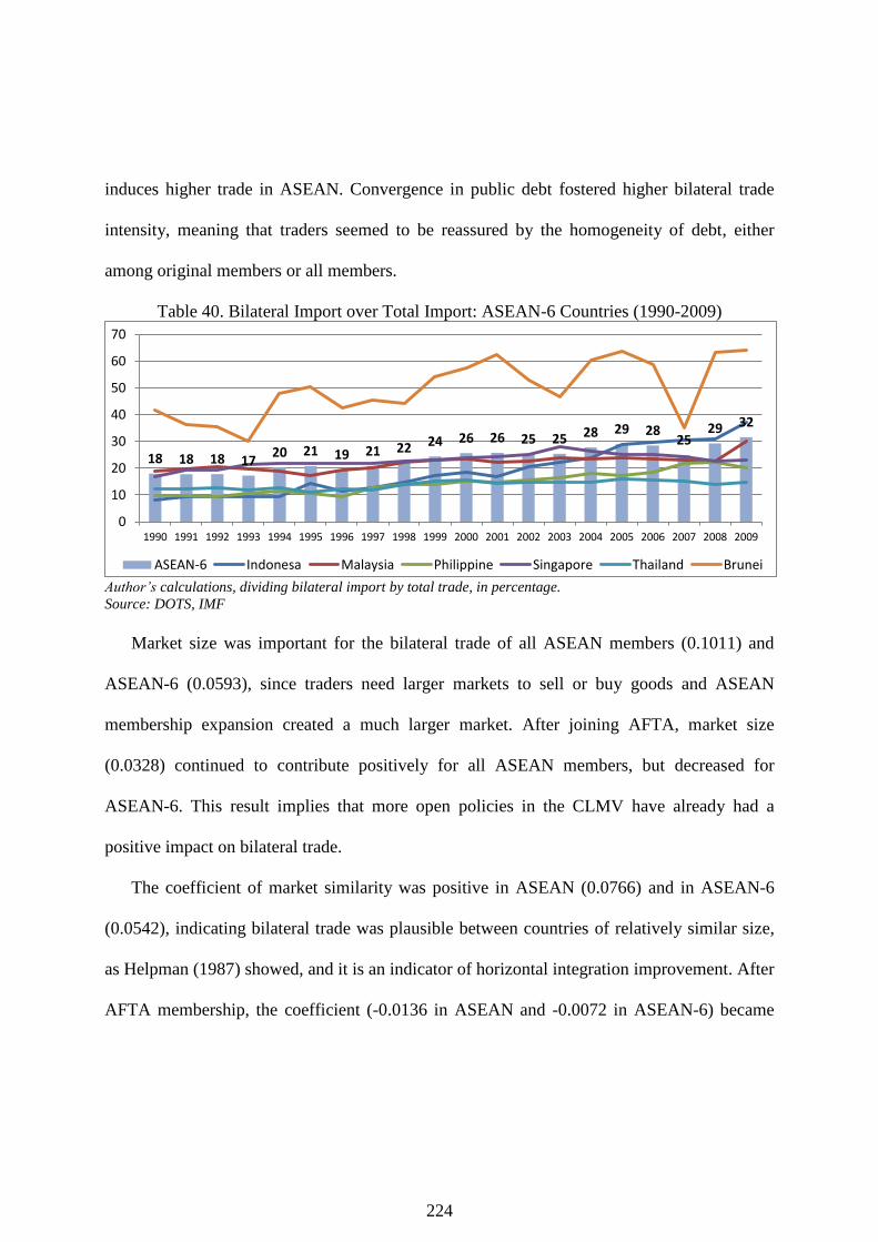
224

induces higher trade in ASEAN. Convergence in public debt fostered higher bilateral trade

intensity, meaning that traders seemed to be reassured by the homogeneity of debt, either

among original members or all members.

Table 40. Bilateral Import over Total Import: ASEAN-6 Countries (1990-2009)

Author’s calculations, dividing bilateral import by total trade, in percentage.

Source: DOTS, IMF

Market size was important for the bilateral trade of all ASEAN members (0.1011) and

ASEAN-6 (0.0593), since traders need larger markets to sell or buy goods and ASEAN

membership expansion created a much larger market. After joining AFTA, market size

(0.0328) continued to contribute positively for all ASEAN members, but decreased for

ASEAN-6. This result implies that more open policies in the CLMV have already had a

positive impact on bilateral trade.

The coefficient of market similarity was positive in ASEAN (0.0766) and in ASEAN-6

(0.0542), indicating bilateral trade was plausible between countries of relatively similar size,

as Helpman (1987) showed, and it is an indicator of horizontal integration improvement. After

AFTA membership, the coefficient (-0.0136 in ASEAN and -0.0072 in ASEAN-6) became

18 18 18 17 20 21 19 21 22 24 26 26 25 25 28 29 28

25 29 32

0

10

20

30

40

50

60

70

1990 1991 1992 1993 1994 1995 1996 1997 1998 1999 2000 2001 2002 2003 2004 2005 2006 2007 2008 2009

ASEAN-6 Indonesa Malaysia Philippine Singapore Thailand Brunei

225

negative, indicating that similarity of market became less important, although the overall

impact was still positive.

Factor endowment was positive when the CLMV was incorporated into the Equation

(0.159). This result implied that differences in factor endowment were important for higher

bilateral trade, and showed the existence of a development gap between ASEAN-6 members

with the CLMV. Since the development stages were relatively similar (the only exceptions

Singapore and Brunei), the endowment impact was insignificant in ASEAN-6. Interacting

with the AFTA dummy, the endowment impact was insignificant in both ASEAN and

ASEAN-6. In line with the gravity hypothesis, the impact of distance was negative in

ASEAN-6 (-0.0333), and even higher for all ASEAN (-0.1023).

7.4.3 Comparative Results

Based on the results in Tables 38 and 39, we present the following comparisons:

Between the Eurozone and ASEAN

Total Trade Weight

When comparing total trade weight, we measured the impact of independent variables

on bilateral trade. We concluded that market size was positively significant in both areas, with

higher influence in ASEAN (0.1011 and 0.0639). A similar result was shown in the impact of

market similarity (0.0766 and 0.0286); however, the pattern was reversed after deeper

integration (-0.0136 and -0.0039). Distance has a negative impact in both regions, higher in

ASEAN (-0.1023 and -0.0369), as did the impact of the crisis (-0.0162 and -0.0044). In regard

226

to other independent variables, differences in inflation, exchange rate, and debt are

insignificant in both regions.

The impact of the euro is positively significant in the Eurozone by 0.0793, but the

impact of AFTA was in reverse (-0.8707). Divergence in interest rates was a positive

influence in the Eurozone (0.0007); while divergence of deficits was only significant in

ASEAN by 0.0018. Differences in factor endowment were positive in ASEAN at 0.0159, but

negative in the Eurozone at -0.0124. Market size continued positive significance in ASEAN

after AFTA (0.0328), but in the Eurozone, after the euro, the result was negative by -0.0033.

Further, factor endowment, after deepening regional integration, only has impacted Eurozone

by 0.0123.

Export Weight

There is little difference in total trade weight. Based on export weight, the impact of

market size (0.1070 and 0.0669) and market similarity (0.0728 and 0.0248) were positive and

significant in both regions, with higher impact in ASEAN. However, after deepening the

integration process, the impact of market similarity was negative in the Eurozone by -0.0039

and in ASEAN by -0.0136. In line with total trade weight, distance (-0.0961 and -0.0324) was

also negative, and higher in ASEAN, as was crisis impact (-0.0224 and -0.0056). The

difference in inflation was insignificant in both regions.

The impact of the euro is positive by 0.0926 for reciprocal export in the Eurozone, and

the influence of AFTA was negative by -0.7078 in ASEAN. Divergence in interest rates was

increased bilateral trade by 0.0015 in the Eurozone. Convergence in exchange rates had a

positive influence by -0.0243 only in the Eurozone.

227

Divergence in deficit (0.0017) and convergence in public debt (-0.0002) are responsible

for higher bilateral trade only between ASEAN members. Factor endowment plays an

important role on higher bilateral trade in ASEAN at 0.0152, but it was insignificant in the

Eurozone. Market size increased bilateral trade by 0.0267 after AFTA in ASEAN, but it

disincentived reciprocal trade by -0.0037 in the Eurozone after the euro. The impact of factor

endowment after the euro was positive by 0.0208, but factor endowment was insignificant in

ASEAN after AFTA.

Import Weight

Related with import weight, the impacts of market size (0.1094 and 0.0611) and market

similarity (0.0732 and 0.0257) are positive and significant, with a greater impact in ASEAN.

The impact of market similarity became insignificant in both regions after deepening regional

economic integration. The impact of distance, as in gravity theory, was negative and

significant by -0.0983 in ASEAN and by -0.0407 in the Eurozone. Convergence in inflation

and exchange rates were insignificant in both regions, but convergence in debt improved

bilateral trade by -0.0002 in ASEAN and by -0.0001 in the Eurozone.

The impact of the euro is positive (0.1064), but the impact of AFTA is negative for

ASEAN (-0.7078), and the crisis discouraged bilateral import by -0.0224 in ASEAN and by -

0.0056 in the Eurozone. Divergence in interest rates led to higher bilateral import in the

Eurozone (0.0010), but it was insignificant in ASEAN. Divergence in deficit increased

bilateral trade in ASEAN by 0.0014. Factor endowment played an important role in ASEAN

(0.0124) but the result was reversed for the Eurozone (-0.0294). However, after the euro‘s

228

launch, the result was positive by 0.0190. Reversed results were also shown in the size of

ASEAN after AFTA (0.0237) and by (-0.0042) in the Eurozone after the euro.

Between the Eurozone and Original members

Total Trade

Based on the results in Table 3, we drew comparisons among all members of the

Eurozone, and among only original members. The result confirmed that both market size

(0.0639 and 0.0579) and market similarity (0.0286 and 0.0271) were positively significant in

both equations, and the impact was greater when NMS was incorporated. However, after the

euro was introduced, the impact change was negative (-0.0039 and -0.0037). Transportation

costs, with distance as a proxy, correlated negatively, -0.0369 between all the Eurozone

members and -0.0251 between only original members. The impact of the crisis was more

painful when NMS was incorporated (-0.0044 and -0.0030). In regard to variables associated

with the MC, differences in inflation, deficit, and debt are insignificant in both equations.

Differences in interest rate have a positive impact on bilateral trade among all members, and

only among original members.

Overall, the impact of the euro is positive by 0.0793, but it was insignificant among

original members. Divergence in exchange rates was influential among original members by

0.0162. Different factor endowment contributes negatively to bilateral trade in the entire

Eurozone, but it was insignificant among original members. After the euro was introduced,

size and similarity were most influential when NMS incorporated (-0.0033 and 0.0123), but

insignificant among original members.

229

Bilateral Export

Weighting with export measure, market size was positive by 0.0669 for all Eurozone

members and by 0.0594 for original members. Market similarity also exhibited a positive

influence of 0.0248 for all members, and 0.0225 for original members, but the impact of

similarity after the euro launch was insignificant in both estimates. Endowment was

insignificant in both equations. Distance was negative in both equations, but with higher

significance when NMS was incorporated, by -0.0324, -0.0222 among original members. The

crisis was painful whether NMS incorporated or not, but the impact was higher when those

countries were incorporated (-0.0056 and -0.0031). Variables related to inflation and debt-to-

GDP ratio are insignificant in both estimates. The divergence in interest rate increased

bilateral trade by 0.0015 in the Eurozone, and by 0.0010 among original members.

The euro‘s impact on export weight is different in both estimations: it was positive

(0.0926) if NMS was incorporated, but insignificant otherwise. Convergence in exchange rate

caused a rise in bilateral exports when NMS incorporated, by -0.0243, but divergence in

nominal exchange rates was preferred if bilateral trade was among members, by 0.0224.

Differences in deficit were insignificant when all members were incorporated, but

convergence in deficits increased bilateral trade among original members by -0.0005. After

the euro launched, market size disincentived bilateral trade, when NMS incorporated, by -

0.0037, but it was insignificant among original members. Endowment impact after the euro

correlated positively when NMS augmented by (0.0208), insignificant among original

members.

230

Bilateral Import

In regard to import weight, market size and market similarity were related positively in

both estimates, although the impact was greater when NMS was incorporated (0.0611 and

0.0576 for market size and 0.0257 and 0.0204 for market similarity); however, market

similarity became insignificant after the euro was introduced. Distance, as hypothesized,

correlated negatively, with greater impact when NMS was augmented (-0.0407 and -0.0226).

During the crisis, reciprocal trade diminished among all Eurozone members by -0.0027,

compared with -0.0024 among original members. Differences in inflation were insignificant

in both estimates, but divergence in interest rates fostered higher bilateral trade in both

estimates, higher when NMS was included (0.0010 and 0.0006).

The impact of the euro was positive by 0.1064 when all members are included, but

insignificant among original members. The difference in exchange rates was insignificant

when NMS is incorporated, but divergence in exchange rates increased bilateral trade by

0.0218. Deficit-to-GDP ratio was insignificant when membership was extended, but

convergence in this variable related with higher reciprocal imports, by -0.0004. Convergence

in debt-to-GDP ratio increases bilateral import when NMS was included, by -0.0001, but it

was insignificant among original members. Different factor endowment correlated negatively

by -0.0294 when all members were included, however the endowment impact reversed after

the euro was introduced. After the euro launched, market size became negative when NMS

incorporated by -0.0042, but insignificant among original members.

231

Between all ASEAN and ASEAN-6

Total Trade

In regard to total trade weight, market size and market similarity have positive and

significant impact on reciprocal bilateral trade, with or without the CLMV incorporated into

the equation; however, when CLMV countries were included, the figures were higher (0.1011

and 0.0593 for market size, and 0.0766 and 0.0542 for market similarity). After AFTA was

introduced, the impact of market similarity became negative by -0.0136 in all ASEAN

countries and -0.0072 in only ASEAN-6 countries. Distance was related negatively by -

0.1023 among all ASEAN members and by -0.0333 among ASEAN-6.

The impact of AFTA was negative for bilateral trade when the CLMV countries were

included, by 0.8707; however, it increased bilateral trade among ASEAN-6 by 0.2853. The

ASEAN economic crisis was influential when CLMV was incorporated by -0.0162.

Divergence in deficit-to-GDP ratio fostered higher bilateral trade, by 0.0018, when the CLMV

countries were included, but convergence in debt-to-GDP ratio was significant only among

original members. Factor endowment was only important for higher bilateral trade intensity

when including CLMV, when the result was 0.0159. The size impact after launching AFTA

was positive for all ASEAN members, by 0.0328, but negative among original members by -

0.0113.

Export Weight

Based on export weight, market size and market similarity impact were positive and

significant, higher when CLMV was incorporated into the equation (0.1070 and 0.0825 for

market size, and 0.0728 and 0.0504 for market similarity). The impact of distance was higher

232

among all ASEAN members by -0.0961 than among ASEAN-6 countries, by -0.0194.

Diminishing differences in variables related with inflation, interest rate, and exchange rate are

insignificant in both ASEAN and ASEAN-6. Factor endowment after AFTA was insignificant

in both estimations.

The impact of AFTA was negative by -0.7078 when CLMV was incorporated into the

equation, and positive by 0.2831 among ASEAN-6. The impact of the crisis was only painful

to bilateral export among all ASEAN members, by -0.0224. Wider differences in deficit were

significant in increasing bilateral trade among all ASEAN members by 0.0017, and

convergence in debt fostered increased bilateral export in all members by -0.0002. Different

factor endowment increases reciprocal trade when the CLMV was incorporated into the

estimate. The size impact after AFTA was positive among all ASEAN members, by 0.0267,

and negative, by -0.0111, in ASEAN-6. After AFTA, the impact of market similarity was

negative in all ASEAN nations, by -0.0144.

Import Weight

Concerning import weight, the impact of market size was positive and significantly

higher among all ASEAN members, by 0.1094, and among ASEAN-6 by 0.0436. A similar

result was found for market similarity: 0.0732 for all ASEAN countries and 0.0605 among

ASEAN-6. Distance was negative, -0.0983 among all ASEAN members and -0.0307 among

ASEAN-6. Differences in inflation, interest, and exchange rates had no significant impact

among ASEAN-6 countries or when the membership was extended. Convergence in debt

increased reciprocal trade by -0.0002 among all ASEAN. After the launch of AFTA, market

233

similarity and factor endowment are insignificant among ASEAN-6 countries and among all

ASEAN members.

The impact of AFTA is negative when CMLV was incorporated, by -0.6385. While the

impact of the crisis was negative when trade occurred among all ASEAN members, by -

0.0132, it was positive when only accounting for ASEAN-6, by 0.0036. Divergence in deficits

fostered higher bilateral imports among all ASEAN members by 0.0014. Factor endowment

raised bilateral import by 0.0124 when CLMV was included into the equation. After AFTA,

country size correlated positively by 0.0237 when the CLMV was incorporated into the

estimation.

7.5 Conclusion and Policy Implication

Using an augmented gravity equation, this paper provides a comparative analysis of

different levels of economic integration on bilateral trade, using two examples, one region

using a common currency (the Eurozone) and the other a struggling free-trade area (ASEAN).

The results show that deepening the level of integration was positive on bilateral trade in all

Eurozone members, but insignificant if for only original members. Thus, expanding

membership increased reciprocal trade. In ASEAN, the creation of AFTA generated a positive

result only among ASEAN-6 members, not when CLMV joined the membership. Thus, the

impact of expansion was negative. The financial crisis reduced the incentive to trade

bilaterally in both the Eurozone (in 2009) and ASEAN (in 1998).

For the Eurozone, in regard to the MC variables, divergence in interest rates creates

incentives for bilateral trade; a similar effect was caused by the divergence of nominal

exchange rates among in original members. A reassuring effect was shown in the deficit-to-

234

GDP ratio for original members, in export and import weight. Thus, it was determined that

forcing convergence in MC variables might be not correlate to an increase in bilateral trade.

For ASEAN, among variables associated with the MC, divergence in deficits increases

bilateral trade, and convergence in debt implies the appearance of the reassuring effect.

Related to H-O variables, the impact of market size, income similarity, and distance

were as expected. Market size and income similarity were important factors for higher flow of

bilateral trade, indicating horizontal linkage creation based predominantly on market access

and consumer income. We found various results for factor endowment impact. Intra-trade

industry was a phenomenon in all Eurozone countries, shown by the negative impact of factor

endowment on bilateral trade, but it was insignificant among original members, due to similar

level of development. For ASEAN, differences in factor endowment were determinant for

higher bilateral trade when CLMV countries were included, as shown by a positive result for

factor endowment; however, among original members, the impact was insignificant.

These results show less impact from the euro, compared to Rose‘s (2000) findings, but

in line with the findings of Sousa (2012). This demonstrates the need for greater economic

integration, as well as measures to decrease trade disputes and friction in the area, especially

regarding trade imbalances. For ASEAN, the result was in line with the problems denoted by

Cuyvers, De Lombaerde, and Verherstraeten (2005), most notably, ASEAN needs to realize

their commitment to lower tariffs based on CEPT scheme, in order to accelerate the

realization of the ASEAN Economic Community by 2015.

235

Appendix 7.1 Bilateral Trade Intensity between the Eurozone Countries Bilateral Trade Intensity Index, Austria as Reporter

Partner 1990 1991 1992 1993 1994 1995 1996 1997 1998 1999 2000 2001 2002 2003 2004 2005 2006 2007 2008 2009 Average

Finland 0.74 0.65 0.65 0.59 0.61 0.67 0.64 0.60 0.78 0.78 0.76 0.71 0.67 0.70 0.58 0.56 0.57 0.51 0.48 0.44 0.63

France 4.43 4.36 4.41 4.48 4.64 4.70 4.56 4.42 4.63 4.61 4.10 4.36 4.17 4.25 4.05 3.95 3.46 3.36 3.39 3.54 4.19 Germany 40.98 41.24 41.52 40.83 39.15 41.16 40.35 38.25 39.48 40.47 38.73 38.03 37.01 37.50 39.19 38.51 37.77 37.64 37.04 38.16 39.15

Ireland 0.27 0.31 0.35 0.37 0.37 0.40 0.39 0.34 0.47 0.44 0.45 0.42 0.40 0.38 0.69 0.35 0.41 0.35 0.36 0.40 0.40

Italy 9.34 9.09 8.70 8.65 8.51 8.81 8.59 8.29 8.50 7.88 7.81 7.68 7.97 8.19 7.84 7.64 7.99 7.97 7.81 7.40 8.23 Netherland 2.85 2.82 2.80 2.96 3.00 3.16 2.92 3.00 2.99 3.55 3.38 3.53 3.45 3.27 2.91 2.78 2.95 3.06 2.96 2.92 3.06

Portugal 0.52 0.53 0.56 0.54 0.54 0.49 0.54 0.51 0.49 0.34 0.35 0.37 0.36 0.37 0.31 0.27 0.29 0.29 0.26 0.29 0.41

Spain 1.50 1.61 1.76 1.71 1.70 1.68 1.81 1.84 2.09 1.98 1.86 1.81 2.28 1.94 1.81 1.91 1.95 1.96 1.70 1.53 1.82

Cyprus 0.04 0.04 0.05 0.03 0.02 0.03 0.02 0.02 0.03 0.02 0.03 0.03 0.07 0.03 0.04 0.04 0.06 0.06 0.05 0.06 0.04

Greece 0.49 0.49 0.51 0.45 0.40 0.43 0.36 0.32 0.33 0.31 0.30 0.33 0.35 0.40 0.34 0.29 0.33 0.38 0.37 0.36 0.38

Malta 0.02 0.02 0.02 0.02 0.02 0.01 0.02 0.02 0.02 0.02 0.02 0.02 0.01 0.01 0.01 0.02 0.10 0.02 0.02 0.02 0.02 Slovakia - - - 0.71 0.76 0.88 1.08 1.18 1.17 1.16 1.23 1.31 1.71 1.82 1.69 1.60 1.66 1.98 2.10 2.17 1.42

Slovenia - - - 1.00 1.06 1.21 1.19 1.31 1.29 1.43 1.48 1.51 1.56 1.69 1.82 1.38 1.50 1.64 1.66 1.69 1.44

Eurozone 61.17 61.15 61.31 62.33 60.77 63.63 62.46 60.11 62.27 63.00 60.49 60.10 60.00 60.56 61.27 59.31 59.03 59.22 58.21 58.97 60.77

Bilateral Trade Intensity Index, Finland as reporter

Partner 1990 1991 1992 1993 1994 1995 1996 1997 1998 1999 2000 2001 2002 2003 2004 2005 2006 2007 2008 2009 Average

Austria 1.23 1.26 1.26 1.10 1.08 1.11 0.97 1.00 1.25 1.21 1.15 1.09 1.10 1.15 0.98 0.85 0.82 0.79 0.76 0.81 1.05 France 5.21 5.07 5.76 5.00 4.62 4.36 4.33 4.47 5.04 4.70 4.49 4.55 4.42 4.02 3.87 3.56 3.31 3.51 3.35 3.93 4.38

Germany 15.21 16.11 16.36 14.52 14.01 14.16 13.36 12.52 13.19 14.28 13.59 13.21 12.96 13.76 13.17 13.35 13.34 13.21 12.77 13.03 13.81

Ireland 0.54 0.63 0.67 0.58 0.58 0.64 0.68 0.80 0.74 0.75 0.69 0.91 0.87 0.66 0.59 0.69 0.67 0.60 0.56 0.60 0.67 Italy 3.90 3.86 3.84 3.47 3.38 3.37 3.19 3.44 3.95 3.58 3.74 3.57 3.45 3.74 3.30 3.16 3.13 2.97 3.00 2.76 3.44

Netherland 3.73 4.21 4.52 4.46 4.45 4.17 3.76 4.05 4.40 5.25 4.94 3.78 4.20 5.48 5.69 5.47 5.77 6.13 5.72 6.43 4.83

Portugal 0.99 1.07 0.99 0.83 0.69 0.64 0.60 0.63 0.62 0.60 0.55 0.52 0.54 0.49 0.48 0.48 0.40 0.35 0.45 0.53 0.62 Spain 1.65 1.96 1.99 1.91 1.87 2.08 1.86 1.85 2.20 2.07 2.01 2.20 2.08 2.14 2.04 1.93 1.91 2.11 2.00 1.70 1.98

Cyprus 0.05 0.04 0.03 0.14 0.03 0.02 0.03 0.03 0.02 0.02 0.02 0.02 0.02 0.02 0.07 0.14 0.05 0.03 0.15 0.23 0.06

Greece 0.47 0.46 0.53 0.43 0.44 0.43 0.41 0.45 0.66 0.55 0.59 0.52 0.56 0.58 0.45 0.37 0.39 0.45 0.38 0.37 0.47

Malta 0.04 0.06 0.02 0.02 0.02 0.02 0.01 0.01 0.01 0.02 0.03 0.03 0.08 0.02 0.02 0.01 0.06 0.06 0.03 0.05 0.03

Slovakia - - - 0.12 0.14 0.14 0.15 0.14 0.16 0.16 0.14 0.16 0.17 0.17 0.17 0.17 0.22 0.23 0.36 0.22 0.18 Slovenia - - - 0.08 0.10 0.09 0.09 0.08 0.08 0.08 0.08 0.08 0.09 0.07 0.09 0.10 0.15 0.14 0.15 0.14 0.10

Eurozone 33.02 34.73 35.99 32.66 31.40 31.23 29.44 29.46 32.32 33.28 32.03 30.64 30.54 32.28 30.92 30.28 30.22 30.58 29.68 30.79 31.57

Bilateral Trade Intensity Index, France as reporter

Partner 1990 1991 1992 1993 1994 1995 1996 1997 1998 1999 2000 2001 2002 2003 2004 2005 2006 2007 2008 2009 Average

Austria 0.86 0.86 0.88 0.93 0.97 0.97 0.94 0.90 0.96 0.93 0.84 0.98 1.05 0.99 0.98 0.92 0.90 0.90 0.89 0.89 0.93

Finland 0.64 0.53 0.57 0.47 0.52 0.56 0.56 0.58 0.63 0.56 0.60 0.57 0.55 0.56 0.52 0.48 0.49 0.51 0.47 0.45 0.54

Germany 17.91 18.00 17.83 17.13 16.96 17.73 16.93 15.69 16.36 17.32 15.32 16.82 17.18 17.48 17.17 16.91 17.30 17.41 17.55 17.78 17.14

Ireland 0.64 0.66 0.77 0.81 0.88 0.87 0.92 1.04 1.22 1.14 1.32 1.18 1.15 1.08 1.07 1.13 1.03 1.02 0.92 1.03 0.99


Portugal 1.27 1.28 1.37 1.30 1.28 1.24 1.22 1.24 1.28 1.33 1.49 1.87 1.51 1.67 1.60 1.08 1.07 1.06 1.02 1.06 1.31 Spain 5.42 5.92 6.20 5.95 6.45 6.81 7.25 7.13 7.82 7.73 7.98 7.62 7.87 8.47 8.40 8.26 8.24 8.12 7.42 7.20 7.31

Cyprus 0.04 0.03 0.06 0.05 0.04 0.04 0.04 0.03 0.03 0.09 0.13 0.12 0.09 0.08 0.05 0.04 0.06 0.05 0.04 0.04 0.06

Greece 0.54 0.51 0.53 0.51 0.46 0.49 0.50 0.51 0.49 0.52 0.54 0.47 0.48 0.57 0.55 0.47 0.49 0.51 0.48 0.48 0.51 Malta 0.05 0.05 0.07 0.07 0.07 0.07 0.11 0.11 0.11 0.11 0.13 0.10 0.11 0.12 0.13 0.10 0.11 0.11 0.10 0.08 0.10

Slovakia - - - 0.04 0.05 0.08 0.10 0.11 0.14 0.11 0.10 0.12 0.15 0.16 0.16 0.19 0.25 0.41 0.45 0.55 0.19

Slovenia - - - 0.24 0.27 0.27 0.30 0.27 0.35 0.24 0.24 0.24 0.28 0.32 0.31 0.31 0.28 0.27 0.27 0.30 0.28

Eurozone 43.86 43.69 43.78 41.85 42.08 43.62 42.99 41.53 43.56 45.04 43.42 44.15 44.76 46.09 45.13 43.64 44.30 44.65 43.42 43.59 43.76

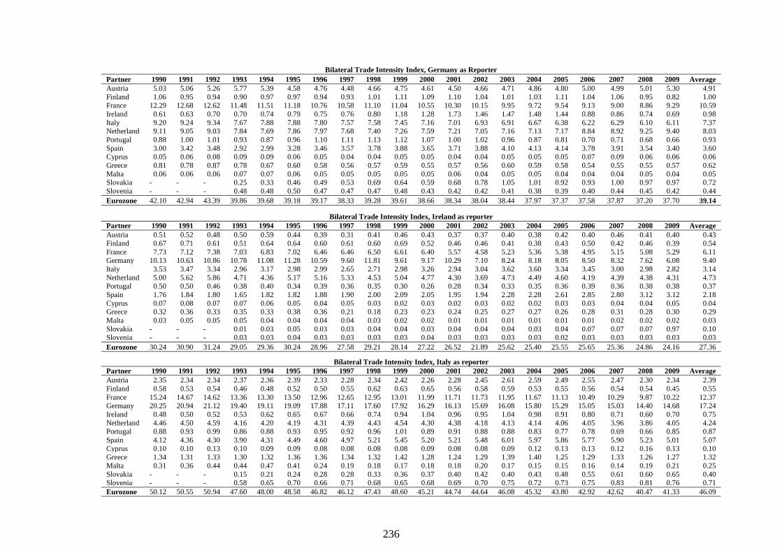
236

Bilateral Trade Intensity Index, Germany as Reporter

Partner 1990 1991 1992 1993 1994 1995 1996 1997 1998 1999 2000 2001 2002 2003 2004 2005 2006 2007 2008 2009 Average

Austria 5.03 5.06 5.26 5.77 5.39 4.58 4.76 4.48 4.66 4.75 4.61 4.50 4.66 4.71 4.86 4.80 5.00 4.99 5.01 5.30 4.91

Finland 1.06 0.95 0.94 0.90 0.97 0.97 0.94 0.93 1.01 1.11 1.09 1.10 1.04 1.01 1.03 1.11 1.04 1.06 0.95 0.82 1.00 France 12.29 12.68 12.62 11.48 11.51 11.18 10.76 10.58 11.10 11.04 10.55 10.30 10.15 9.95 9.72 9.54 9.13 9.00 8.86 9.29 10.59

Ireland 0.61 0.63 0.70 0.70 0.74 0.79 0.75 0.76 0.80 1.18 1.28 1.73 1.46 1.47 1.48 1.44 0.88 0.86 0.74 0.69 0.98


Portugal 0.88 1.00 1.01 0.93 0.87 0.96 1.10 1.11 1.13 1.12 1.07 1.00 1.02 0.96 0.87 0.81 0.70 0.71 0.68 0.66 0.93

Spain 3.00 3.42 3.48 2.92 2.99 3.28 3.46 3.57 3.78 3.88 3.65 3.71 3.88 4.10 4.13 4.14 3.78 3.91 3.54 3.40 3.60 Cyprus 0.05 0.06 0.08 0.09 0.09 0.06 0.05 0.04 0.04 0.05 0.05 0.04 0.04 0.05 0.05 0.05 0.07 0.09 0.06 0.06 0.06

Greece 0.81 0.78 0.87 0.78 0.67 0.60 0.58 0.56 0.57 0.59 0.55 0.57 0.56 0.60 0.59 0.58 0.54 0.55 0.55 0.57 0.62

Malta 0.06 0.06 0.06 0.07 0.07 0.06 0.05 0.05 0.05 0.05 0.05 0.06 0.04 0.05 0.05 0.04 0.04 0.04 0.05 0.04 0.05 Slovakia - - - 0.25 0.33 0.46 0.49 0.53 0.69 0.64 0.59 0.68 0.78 1.05 1.01 0.92 0.93 1.00 0.97 0.97 0.72

Slovenia - - - 0.48 0.48 0.50 0.47 0.47 0.47 0.48 0.43 0.42 0.42 0.41 0.38 0.39 0.40 0.44 0.45 0.42 0.44

Eurozone 42.10 42.94 43.39 39.86 39.68 39.18 39.17 38.33 39.28 39.61 38.66 38.34 38.04 38.44 37.97 37.37 37.58 37.87 37.20 37.70 39.14

Bilateral Trade Intensity Index, Ireland as reporter

Partner 1990 1991 1992 1993 1994 1995 1996 1997 1998 1999 2000 2001 2002 2003 2004 2005 2006 2007 2008 2009 Average

Austria 0.51 0.52 0.48 0.50 0.59 0.44 0.39 0.31 0.41 0.46 0.43 0.37 0.37 0.40 0.38 0.42 0.40 0.46 0.41 0.40 0.43

Finland 0.67 0.71 0.61 0.51 0.64 0.64 0.60 0.61 0.60 0.69 0.52 0.46 0.46 0.41 0.38 0.43 0.50 0.42 0.46 0.39 0.54

France 7.73 7.12 7.38 7.03 6.83 7.02 6.46 6.46 6.50 6.61 6.40 5.57 4.58 5.23 5.36 5.38 4.95 5.15 5.08 5.29 6.11 Germany 10.13 10.63 10.86 10.78 11.08 11.28 10.59 9.60 11.81 9.61 9.17 10.29 7.10 8.24 8.18 8.05 8.50 8.32 7.62 6.08 9.40

Italy 3.53 3.47 3.34 2.96 3.17 2.98 2.99 2.65 2.71 2.98 3.26 2.94 3.04 3.62 3.60 3.34 3.45 3.00 2.98 2.82 3.14

Netherland 5.00 5.62 5.86 4.71 4.36 5.17 5.16 5.33 4.53 5.04 4.77 4.30 3.69 4.73 4.49 4.60 4.19 4.39 4.38 4.31 4.73

Portugal 0.50 0.50 0.46 0.38 0.40 0.34 0.39 0.36 0.35 0.30 0.26 0.28 0.34 0.33 0.35 0.36 0.39 0.36 0.38 0.38 0.37

Spain 1.76 1.84 1.80 1.65 1.82 1.82 1.88 1.90 2.00 2.09 2.05 1.95 1.94 2.28 2.28 2.61 2.85 2.80 3.12 3.12 2.18

Cyprus 0.07 0.08 0.07 0.07 0.06 0.05 0.04 0.05 0.03 0.02 0.03 0.02 0.03 0.02 0.02 0.03 0.03 0.04 0.04 0.05 0.04 Greece 0.32 0.36 0.33 0.35 0.33 0.38 0.36 0.21 0.18 0.23 0.23 0.24 0.25 0.27 0.27 0.26 0.28 0.31 0.28 0.30 0.29

Malta 0.03 0.05 0.05 0.05 0.04 0.04 0.04 0.04 0.03 0.02 0.02 0.01 0.01 0.01 0.01 0.01 0.01 0.02 0.02 0.02 0.03


Eurozone 30.24 30.90 31.24 29.05 29.36 30.24 28.96 27.58 29.21 28.14 27.22 26.52 21.89 25.62 25.40 25.55 25.65 25.36 24.86 24.16 27.36

Bilateral Trade Intensity Index, Italy as reporter

Partner 1990 1991 1992 1993 1994 1995 1996 1997 1998 1999 2000 2001 2002 2003 2004 2005 2006 2007 2008 2009 Average

Austria 2.35 2.34 2.34 2.37 2.36 2.39 2.33 2.28 2.34 2.42 2.26 2.28 2.45 2.61 2.59 2.49 2.55 2.47 2.30 2.34 2.39

Finland 0.58 0.53 0.54 0.46 0.48 0.52 0.50 0.55 0.62 0.63 0.65 0.56 0.58 0.59 0.53 0.55 0.56 0.54 0.54 0.45 0.55

France 15.24 14.67 14.62 13.36 13.30 13.50 12.96 12.65 12.95 13.01 11.99 11.71 11.73 11.95 11.67 11.13 10.49 10.29 9.87 10.22 12.37 Germany 20.25 20.94 21.12 19.40 19.11 19.09 17.88 17.11 17.60 17.92 16.29 16.13 15.69 16.08 15.80 15.29 15.05 15.03 14.40 14.68 17.24

Ireland 0.48 0.50 0.52 0.53 0.62 0.65 0.67 0.66 0.74 0.94 1.04 0.96 0.95 1.04 0.98 0.91 0.80 0.71 0.60 0.70 0.75

Netherland 4.46 4.50 4.59 4.16 4.20 4.19 4.31 4.39 4.43 4.54 4.30 4.38 4.18 4.13 4.14 4.06 4.05 3.96 3.86 4.05 4.24 Portugal 0.88 0.93 0.99 0.86 0.88 0.93 0.95 0.92 0.96 1.01 0.89 0.91 0.88 0.88 0.83 0.77 0.78 0.69 0.66 0.85 0.87

Spain 4.12 4.36 4.30 3.90 4.31 4.49 4.60 4.97 5.21 5.45 5.20 5.21 5.48 6.01 5.97 5.86 5.77 5.90 5.23 5.01 5.07

Cyprus 0.10 0.10 0.13 0.10 0.09 0.09 0.08 0.08 0.08 0.08 0.09 0.08 0.08 0.09 0.12 0.13 0.13 0.12 0.16 0.13 0.10 Greece 1.34 1.31 1.33 1.30 1.32 1.36 1.36 1.34 1.32 1.42 1.28 1.24 1.29 1.39 1.40 1.25 1.29 1.33 1.26 1.27 1.32

Malta 0.31 0.36 0.44 0.44 0.47 0.41 0.24 0.19 0.18 0.17 0.18 0.18 0.20 0.17 0.15 0.15 0.16 0.14 0.19 0.21 0.25


Eurozone 50.12 50.55 50.94 47.60 48.00 48.58 46.82 46.12 47.43 48.60 45.21 44.74 44.64 46.08 45.32 43.80 42.92 42.62 40.47 41.33 46.09

237

Bilateral Trade Intensity Index, Netherland as reporter

Partner 1990 1991 1992 1993 1994 1995 1996 1997 1998 1999 2000 2001 2002 2003 2004 2005 2006 2007 2008 2009 Average

Austria 1.05 1.03 1.08 1.11 1.07 1.16 1.17 1.12 1.27 1.07 1.05 1.16 1.07 1.12 1.08 0.99 0.99 1.01 0.97 0.95 1.08

Finland 0.91 0.79 0.75 0.79 0.88 0.90 0.84 0.89 0.93 0.92 0.96 0.95 0.97 0.98 1.04 1.02 1.03 1.01 0.91 0.86 0.92 France 9.52 9.18 9.32 8.80 9.01 9.03 8.94 8.77 8.82 8.45 8.09 8.18 7.99 7.79 7.56 7.16 6.66 6.53 6.76 6.97 8.18

Germany 26.20 27.62 27.50 25.51 25.53 25.12 24.57 22.88 21.84 22.35 21.63 22.23 21.69 21.84 21.72 20.99 21.49 21.25 21.24 21.59 23.24

Ireland 0.73 0.69 0.85 0.90 0.88 0.96 0.85 1.04 1.08 1.25 1.18 1.30 1.24 1.43 1.21 1.12 1.01 1.01 0.89 0.90 1.03 Italy 5.19 5.10 5.07 4.52 4.55 4.47 4.60 4.49 4.36 4.39 4.32 4.53 4.49 4.42 4.32 4.09 3.75 3.69 3.68 3.64 4.38

Portugal 0.69 0.69 0.71 0.73 0.65 0.66 0.66 0.66 0.70 0.70 0.67 0.70 0.69 0.71 0.66 0.66 0.57 0.54 0.53 0.57 0.66

Spain 2.10 2.10 2.21 2.24 2.27 2.48 2.52 2.69 2.84 2.74 2.71 2.84 2.84 3.00 3.07 3.00 2.73 2.75 2.56 2.60 2.61 Cyprus 0.04 0.04 0.04 0.05 0.05 0.03 0.03 0.03 0.03 0.03 0.03 0.03 0.03 0.04 0.04 0.06 0.06 0.05 0.06 0.07 0.04

Greece 0.59 0.60 0.64 0.61 0.61 0.56 0.50 0.46 0.47 0.47 0.50 0.50 0.53 0.52 0.50 0.47 0.43 0.44 0.44 0.46 0.51

Malta 0.03 0.03 0.03 0.04 0.03 0.03 0.03 0.03 0.03 0.02 0.02 0.03 0.02 0.02 0.02 0.02 0.03 0.02 0.02 0.05 0.03 Slovakia - - - 0.07 0.08 0.09 0.10 0.12 0.14 0.11 0.10 0.12 0.14 0.14 0.19 0.21 0.24 0.35 0.34 0.36 0.17

Slovenia - - - 0.11 0.10 0.10 0.09 0.10 0.12 0.09 0.10 0.10 0.11 0.11 0.10 0.10 0.12 0.12 0.12 0.12 0.11

Eurozone 47.05 47.87 48.19 45.48 45.72 45.60 44.91 43.27 42.62 42.60 41.36 42.66 41.80 42.13 41.52 39.89 39.10 38.78 38.52 39.16 42.91

Bilateral Trade Intensity Index, Netherland as reporter

Partner 1990 1991 1992 1993 1994 1995 1996 1997 1998 1999 2000 2001 2002 2003 2004 2005 2006 2007 2008 2009 Average

Austria 1.05 1.03 1.08 1.11 1.07 1.16 1.17 1.12 1.27 1.07 1.05 1.16 1.07 1.12 1.08 0.99 0.99 1.01 0.97 0.95 1.08 Finland 0.91 0.79 0.75 0.79 0.88 0.90 0.84 0.89 0.93 0.92 0.96 0.95 0.97 0.98 1.04 1.02 1.03 1.01 0.91 0.86 0.92

France 9.52 9.18 9.32 8.80 9.01 9.03 8.94 8.77 8.82 8.45 8.09 8.18 7.99 7.79 7.56 7.16 6.66 6.53 6.76 6.97 8.18

Germany 26.20 27.62 27.50 25.51 25.53 25.12 24.57 22.88 21.84 22.35 21.63 22.23 21.69 21.84 21.72 20.99 21.49 21.25 21.24 21.59 23.24 Ireland 0.73 0.69 0.85 0.90 0.88 0.96 0.85 1.04 1.08 1.25 1.18 1.30 1.24 1.43 1.21 1.12 1.01 1.01 0.89 0.90 1.03

Italy 5.19 5.10 5.07 4.52 4.55 4.47 4.60 4.49 4.36 4.39 4.32 4.53 4.49 4.42 4.32 4.09 3.75 3.69 3.68 3.64 4.38

Portugal 0.69 0.69 0.71 0.73 0.65 0.66 0.66 0.66 0.70 0.70 0.67 0.70 0.69 0.71 0.66 0.66 0.57 0.54 0.53 0.57 0.66 Spain 2.10 2.10 2.21 2.24 2.27 2.48 2.52 2.69 2.84 2.74 2.71 2.84 2.84 3.00 3.07 3.00 2.73 2.75 2.56 2.60 2.61

Cyprus 0.04 0.04 0.04 0.05 0.05 0.03 0.03 0.03 0.03 0.03 0.03 0.03 0.03 0.04 0.04 0.06 0.06 0.05 0.06 0.07 0.04

Greece 0.59 0.60 0.64 0.61 0.61 0.56 0.50 0.46 0.47 0.47 0.50 0.50 0.53 0.52 0.50 0.47 0.43 0.44 0.44 0.46 0.51 Malta 0.03 0.03 0.03 0.04 0.03 0.03 0.03 0.03 0.03 0.02 0.02 0.03 0.02 0.02 0.02 0.02 0.03 0.02 0.02 0.05 0.03

Slovakia - - - 0.07 0.08 0.09 0.10 0.12 0.14 0.11 0.10 0.12 0.14 0.14 0.19 0.21 0.24 0.35 0.34 0.36 0.17

Slovenia - - - 0.11 0.10 0.10 0.09 0.10 0.12 0.09 0.10 0.10 0.11 0.11 0.10 0.10 0.12 0.12 0.12 0.12 0.11

Eurozone 47.05 47.87 48.19 45.48 45.72 45.60 44.91 43.27 42.62 42.60 41.36 42.66 41.80 42.13 41.52 39.89 39.10 38.78 38.52 39.16 42.91

Bilateral Trade Intensity Index, Portugal as reporter

Partner 1990 1991 1992 1993 1994 1995 1996 1997 1998 1999 2000 2001 2002 2003 2004 2005 2006 2007 2008 2009 Average

Austria 0.90 0.95 0.82 0.96 0.90 0.77 0.86 0.81 0.74 0.76 0.69 0.67 0.73 0.72 0.67 0.61 0.58 0.73 0.54 0.70 0.76

Finland 1.03 1.02 0.87 0.78 0.70 0.71 0.64 0.68 0.70 0.67 0.50 0.47 0.49 0.54 0.58 0.64 0.50 0.49 0.58 0.62 0.66

France 12.95 12.48 13.11 13.60 13.52 12.74 12.33 11.96 12.43 12.38 11.37 11.19 11.17 11.15 11.15 10.28 9.64 9.92 9.21 9.90 11.62

Germany 15.30 16.20 16.34 16.71 15.84 17.53 17.85 16.84 16.82 16.65 15.19 15.97 16.35 14.69 13.95 12.87 13.04 12.87 12.00 12.63 15.28

Ireland 0.45 0.42 0.40 0.50 0.60 0.50 0.51 0.56 0.60 0.64 0.55 0.58 0.63 0.66 0.71 0.78 0.74 0.67 0.81 0.73 0.60 Italy 7.58 7.58 7.69 6.44 6.46 6.33 6.40 6.26 6.40 6.39 5.85 5.90 5.86 5.76 5.38 4.85 4.93 4.76 4.45 4.86 6.01

Netherland 5.70 5.78 6.23 5.01 4.78 4.88 4.62 4.55 4.86 4.64 4.44 4.59 4.23 4.32 4.36 4.14 4.11 4.06 3.91 4.65 4.69

Spain 14.20 15.08 15.70 16.52 17.75 18.74 19.14 19.06 20.67 22.51 23.03 23.44 24.97 27.58 27.55 27.80 27.99 28.54 27.67 29.54 22.37 Cyprus 0.05 0.04 0.05 0.05 0.04 0.03 0.03 0.00 0.03 0.02 0.03 0.03 0.02 0.03 0.02 0.02 0.03 0.03 0.04 0.03 0.03

Greece 0.27 0.21 0.24 0.27 0.25 0.26 0.30 0.23 0.24 0.28 0.27 0.28 0.28 0.29 0.26 0.27 0.24 0.25 0.25 0.25 0.26

Malta 0.02 0.02 0.03 0.02 0.03 0.12 0.02 0.02 0.02 0.01 0.03 0.04 0.02 0.03 0.02 0.03 0.02 0.02 0.03 0.03 0.03 Slovakia - - - 0.02 0.02 0.03 0.05 0.04 0.03 0.02 0.04 0.08 0.08 0.08 0.08 0.08 0.10 0.16 0.14 0.19 0.07

Slovenia - - - 0.04 0.03 0.03 0.04 0.02 0.03 0.03 0.03 0.04 0.04 0.04 0.05 0.06 0.06 0.06 0.06 0.06 0.04

Eurozone 58.47 59.78 61.47 60.92 60.92 62.67 62.79 61.04 63.56 65.01 62.03 63.26 64.88 65.89 64.79 62.44 61.96 62.58 59.69 64.19 62.42

238

Trade Intensity Index, Spain as reporter

Partner 1990 1991 1992 1993 1994 1995 1996 1997 1998 1999 2000 2001 2002 2003 2004 2005 2006 2007 2008 2009 Average

Austria 0.78 0.73 0.81 0.95 0.96 0.85 0.93 0.95 0.97 1.06 0.97 1.02 1.07 1.04 0.97 0.84 0.83 0.90 0.84 0.84 0.91

Finland 0.62 0.57 0.57 0.60 0.64 0.66 0.57 0.58 0.61 0.63 0.65 0.57 0.55 0.59 0.54 0.50 0.54 0.58 0.54 0.41 0.58

France 17.01 16.65 17.60 17.90 18.64 18.59 18.88 17.88 18.88 18.87 18.36 17.91 17.83 17.87 17.39 16.55 15.50 15.22 14.56 15.60 17.38 Germany 15.33 15.76 16.14 15.41 14.42 15.29 14.68 14.18 14.68 14.87 13.87 14.12 14.30 14.72 14.65 13.72 13.28 14.01 13.04 13.33 14.49

Ireland 0.55 0.59 0.65 0.67 0.71 0.75 0.69 0.84 0.97 1.04 1.11 1.04 1.09 1.03 1.00 1.10 1.13 1.05 1.04 1.13 0.91


Portugal 3.87 4.14 4.60 4.84 5.00 5.31 5.52 5.61 5.74 5.68 5.29 5.66 5.82 6.01 6.00 5.81 5.53 5.44 5.69 6.02 5.38

Cyprus 0.03 0.06 0.06 0.04 0.03 0.05 0.05 0.08 0.08 0.05 0.07 0.06 0.06 0.06 0.05 0.05 0.05 0.05 0.08 0.06 0.06 Greece 0.44 0.44 0.42 0.50 0.55 0.63 0.64 0.56 0.51 0.55 0.56 0.59 0.63 0.69 0.63 0.58 0.60 0.63 0.64 0.58 0.57

Malta 0.02 0.03 0.03 0.06 0.03 0.06 0.07 0.05 0.06 0.04 0.07 0.04 0.08 0.05 0.04 0.03 0.03 0.04 0.04 0.06 0.05


Eurozone 53.43 52.92 54.95 53.97 54.13 55.54 55.09 54.30 56.15 56.29 54.01 54.05 54.82 56.12 54.98 52.25 50.59 51.37 48.99 50.41 53.72

Bilateral Trade Intensity Index, Cyprus as reporter

Partner 1990 1991 1992 1993 1994 1995 1996 1997 1998 1999 2000 2001 2002 2003 2004 2005 2006 2007 2008 2009 Average

Austria 0.93 1.11 1.25 0.80 0.54 0.68 0.52 0.49 0.79 0.70 0.67 0.57 0.62 0.62 0.68 0.53 0.60 0.60 0.55 0.61 0.69 Finland 0.34 0.54 0.35 0.36 0.49 0.35 0.42 0.46 0.43 0.61 0.45 0.59 0.65 0.62 1.25 2.69 0.82 0.35 0.29 0.36 0.62

France 5.21 3.18 6.30 4.73 3.60 3.44 3.25 3.41 4.14 4.40 3.90 5.41 4.47 4.41 5.61 6.35 4.83 4.78 3.64 3.59 4.43

Germany 7.79 7.92 7.74 7.30 7.37 7.10 6.34 5.27 7.36 6.14 6.42 5.73 7.72 6.72 8.27 7.88 8.32 8.98 7.97 8.84 7.36 Ireland 0.70 0.81 0.67 0.78 0.74 0.71 0.58 0.62 0.76 0.79 0.84 0.67 0.70 0.69 0.58 0.56 0.58 0.54 0.42 0.45 0.66

Italy 7.69 7.92 7.56 8.05 7.75 7.69 7.16 6.48 7.46 7.40 7.58 6.97 8.07 8.39 9.02 8.55 10.15 9.21 9.69 9.48 8.11

Netherland 2.33 1.93 2.15 2.26 2.60 1.89 1.60 1.62 2.00 2.18 2.12 1.92 2.20 2.45 3.17 3.62 3.84 3.73 3.72 4.38 2.59 Portugal 0.30 0.39 0.36 0.35 0.34 0.32 0.31 0.30 0.39 0.34 0.39 0.29 0.35 0.47 0.42 0.33 0.40 0.40 0.44 0.36 0.36

Spain 1.86 1.41 1.68 1.96 2.05 1.85 1.88 2.07 2.96 2.54 3.21 3.28 3.16 3.49 3.16 2.77 2.53 3.15 3.42 3.19 2.58

Greece 7.76 7.27 6.96 8.14 7.07 6.90 6.82 7.16 8.55 8.45 8.83 8.53 9.33 11.49 14.63 16.33 17.01 18.13 17.42 20.69 10.87 Malta 1.84 1.62 1.80 1.92 2.36 1.56 1.28 1.37 1.63 1.74 1.79 1.66 1.82 2.07 2.85 3.27 3.65 3.56 3.57 4.24 2.28

Slovakia - - - - 0.11 0.18 0.12 0.11 0.11 0.12 0.15 0.19 0.13 0.20 0.18 0.14 0.19 0.21 0.13 0.09 0.15 Slovenia - - - 0.08 0.09 0.09 0.20 0.08 0.27 0.41 0.00 0.13 0.13 0.09 0.22 0.41 0.06 0.09 0.09 0.07 0.15

Eurozone 36.74 34.10 36.82 36.73 35.11 32.77 30.48 29.45 36.85 35.83 36.34 35.94 39.35 41.70 50.04 53.43 52.98 53.72 51.37 56.34 40.80

Bilateral Trade Intensity Index, Greece as reporter

Partner 1990 1991 1992 1993 1994 1995 1996 1997 1998 1999 2000 2001 2002 2003 2004 2005 2006 2007 2008 2009 Average

Austria 1.39 1.35 1.49 1.21 1.22 1.07 1.18 1.05 1.07 1.01 0.84 0.76 0.76 0.96 1.05 1.01 1.06 1.18 1.17 1.27 1.11

Finland 0.77 0.73 0.61 0.62 0.81 0.74 0.72 0.78 0.94 1.13 1.48 0.87 0.79 1.07 0.95 0.83 0.98 0.85 0.89 0.80 0.87

France 8.53 7.70 7.76 6.70 7.10 7.41 7.03 7.55 7.58 7.79 5.95 5.68 5.14 6.15 5.88 5.34 5.56 5.23 4.85 5.50 6.52

Germany 21.20 20.70 21.33 18.65 17.64 18.30 15.48 15.41 16.15 15.26 13.21 13.10 11.69 12.73 13.25 12.70 12.24 12.53 11.61 13.06 15.31

Ireland 0.48 0.45 0.51 0.56 0.60 0.82 0.70 0.61 0.61 0.68 0.86 0.75 0.55 0.73 0.74 0.75 0.75 0.80 0.75 0.91 0.68 Italy 15.91 14.94 15.53 13.47 15.04 17.47 15.74 15.65 15.08 15.03 12.04 11.14 10.74 12.15 12.22 11.89 11.43 11.47 11.49 12.28 13.54

Netherland 5.79 5.25 5.74 5.41 5.77 5.71 5.20 5.12 5.42 5.47 5.17 4.80 4.79 4.69 4.88 4.74 4.41 4.29 4.25 5.15 5.10

Portugal 0.37 0.31 0.36 0.31 0.34 0.39 0.49 0.38 0.37 0.38 0.39 0.39 0.34 0.35 0.37 0.34 0.31 0.32 0.34 0.36 0.36 Spain 1.86 2.04 2.28 2.33 2.71 3.43 3.34 3.08 3.39 3.36 3.39 3.32 3.52 3.66 3.69 3.85 3.67 3.56 3.39 3.68 3.18

Cyprus 0.93 0.98 1.14 1.49 1.22 1.10 1.18 1.11 1.15 1.21 1.53 1.44 1.36 1.30 1.41 1.75 1.95 2.39 2.26 2.91 1.49 Malta 0.16 0.19 0.19 0.67 0.46 0.27 0.28 0.32 0.27 0.31 0.35 0.42 0.32 0.12 0.08 0.04 0.04 0.05 0.08 0.09 0.24

Slovakia - - - 0.14 0.10 0.11 0.13 0.13 0.12 0.10 0.11 0.20 0.17 0.17 0.18 0.15 0.24 0.30 0.19 0.26 0.16

Slovenia - - - 0.08 0.09 0.19 0.10 0.11 0.11 0.11 0.11 0.15 0.13 0.14 0.17 0.15 0.42 0.41 0.44 0.32 0.19

Eurozone 57.37 54.64 56.94 51.64 53.10 57.01 51.57 51.29 52.25 51.83 45.45 43.01 40.30 44.23 44.88 43.54 43.04 43.38 41.70 46.58 48.69

239

Trade Intensity Index,Malta as reporter

Partner 1990 1991 1992 1993 1994 1995 1996 1997 1998 1999 2000 2001 2002 2003 2004 2005 2006 2007 2008 2009 Average

Austria 0.87 0.43 0.35 0.33 0.34 0.35 0.35 0.40 0.42 0.36 0.39 0.42 0.44 0.48 0.43 0.51 0.56 0.62 0.82 0.44 0.47

Finland 0.16 0.09 0.19 0.08 0.09 0.07 0.12 0.11 0.07 0.18 0.40 0.35 0.26 0.26 0.27 0.16 1.01 0.90 0.55 0.70 0.30

France 7.18 7.36 7.40 9.14 8.94 9.87 15.47 17.57 12.68 17.52 14.33 9.64 14.87 15.35 14.08 11.70 12.93 12.02 9.69 9.50 11.86 Germany 15.03 13.54 12.12 14.81 16.26 13.28 11.32 11.32 8.92 11.05 8.80 8.75 8.78 8.88 9.65 10.52 9.64 10.41 10.07 10.32 11.17

Ireland 0.49 0.66 0.66 0.68 0.51 0.55 0.64 0.72 0.57 0.55 0.62 0.26 0.55 0.47 0.48 0.46 0.33 0.53 0.53 0.66 0.55


Portugal 0.24 0.20 0.34 0.20 0.24 0.30 0.21 0.25 0.22 0.18 0.20 0.34 0.30 0.34 0.32 0.29 0.98 0.28 0.25 0.26 0.30

Spain 1.12 1.07 1.14 1.02 1.23 1.35 1.21 1.46 2.73 1.35 1.22 1.58 1.77 1.91 2.16 2.33 2.19 1.96 2.23 2.64 1.68 Cyprus 0.06 0.08 0.07 0.06 0.09 0.04 0.06 0.05 0.04 0.04 0.06 0.26 0.05 0.06 0.08 0.12 0.14 0.14 0.24 0.18 0.10

Greece 0.64 0.57 0.47 0.52 0.56 0.50 0.48 0.47 0.41 0.35 0.28 2.51 0.39 0.31 0.43 0.42 0.44 0.54 0.62 0.77 0.58


Eurozone 61.53 62.97 64.35 58.69 61.26 57.00 49.14 49.44 43.83 45.55 39.14 39.49 43.22 44.59 46.71 50.44 49.28 46.83 47.22 45.24 50.30

Bilateral Trade Intensity Index, Slovakia as reporter

Partner 1990 1991 1992 1993 1994 1995 1996 1997 1998 1999 2000 2001 2002 2003 2004 2005 2006 2007 2008 2009 Average

Austria - - - 5.67 5.52 5.04 5.25 5.92 5.86 6.27 5.97 5.88 5.74 8.03 7.35 6.67 5.78 5.56 5.43 5.47 5.97

Finland - - - 0.10 0.17 0.23 0.18 0.17 0.17 0.20 0.20 0.18 0.23 0.13 0.18 0.36 0.52 0.38 0.69 0.18 0.25 France - - - 1.55 1.97 2.24 2.73 3.09 3.67 4.27 3.94 3.90 4.31 3.00 2.69 3.50 3.74 5.27 5.16 6.24 3.60

Germany - - - 13.08 15.19 16.40 17.36 21.40 27.01 26.81 25.84 25.71 24.11 31.76 29.93 24.98 22.78 21.14 19.66 18.91 22.48

Ireland - - - 0.10 0.15 0.14 0.18 0.22 0.23 0.24 0.21 0.25 0.25 0.15 0.13 0.20 0.24 0.22 0.18 0.15 0.19 Italy - - - 2.88 4.35 4.72 5.50 5.90 6.78 7.89 7.57 7.48 8.61 5.49 5.55 5.53 5.36 5.07 4.77 5.18 5.80

Netherland - - - 1.43 1.72 1.74 1.85 2.03 2.16 2.34 2.05 2.06 2.32 1.85 2.32 2.89 3.20 2.86 2.71 2.82 2.26

Portugal - - - 0.03 0.07 0.08 0.06 0.10 0.11 0.10 0.12 0.21 0.26 0.14 0.13 0.15 0.16 0.24 0.23 0.25 0.14 Spain - - - 0.38 0.60 0.71 0.76 0.88 1.02 1.18 1.63 1.89 2.47 1.99 1.34 1.69 1.98 2.14 1.69 1.73 1.42

Cyprus - - - 0.04 0.06 0.07 0.05 0.04 0.03 0.03 0.03 0.05 0.03 0.02 0.02 0.11 0.07 0.13 0.07 0.08 0.05 Greece - - - 0.29 0.22 0.21 0.21 0.22 0.19 0.21 0.19 0.37 0.24 0.22 0.21 0.24 0.35 0.39 0.34 0.44 0.27

Malta - - - 0.04 0.01 0.01 0.01 0.01 0.01 0.01 0.01 0.03 0.01 0.00 0.00 0.00 0.00 0.01 0.01 0.01 0.01

Slovenia - - - 0.54 0.56 0.82 0.72 0.71 0.69 0.73 0.79 0.77 0.92 0.84 0.74 0.80 0.69 0.70 0.89 0.78 0.75

Eurozone - - - 26.13 30.59 32.39 34.87 40.70 47.93 50.29 48.54 48.78 49.48 53.63 50.61 47.13 44.88 44.11 41.84 42.24 43.18

Bilateral Trade Intensity Index,Slovenia as reporter

Partner 1990 1991 1992 1993 1994 1995 1996 1997 1998 1999 2000 2001 2002 2003 2004 2005 2006 2007 2008 2009 Average

Austria - - - 6.53 7.40 8.06 7.81 7.64 7.41 7.72 7.90 7.95 7.67 8.01 13.44 9.96 10.08 9.60 9.43 9.55 8.60

Finland - - - 0.27 0.38 0.32 0.33 0.33 0.32 0.38 0.43 0.43 0.44 0.43 0.30 0.27 0.33 0.32 0.33 0.30 0.35

France - - - 8.01 7.86 8.20 8.58 8.14 10.48 8.56 8.82 8.83 8.49 7.94 9.01 7.49 6.04 5.44 5.16 6.17 7.84 Germany - - - 26.12 24.92 26.14 25.87 24.81 24.31 25.10 22.78 22.65 21.86 21.14 19.23 19.35 19.31 18.38 17.89 17.95 22.22

Ireland - - - 0.30 0.16 0.20 0.19 0.18 0.21 0.26 0.27 0.26 0.23 0.28 0.15 0.18 0.17 0.16 0.14 0.22 0.21

Italy - - - 13.79 14.30 15.65 15.20 15.81 15.41 15.43 15.66 15.23 15.07 15.83 15.96 15.50 15.17 14.82 14.25 13.67 15.10 Netherland - - - 1.62 1.75 1.80 1.80 1.82 1.92 1.91 1.92 1.82 1.87 1.93 2.18 2.46 2.47 2.44 2.30 2.27 2.02

Portugal - - - 0.14 0.07 0.08 0.10 0.13 0.14 0.12 0.15 0.15 0.18 0.18 0.13 0.29 0.26 0.22 0.19 0.19 0.16

Spain - - - 0.91 0.99 1.48 1.21 1.42 1.58 1.58 1.85 1.83 2.09 1.76 1.86 2.38 2.19 2.00 1.84 1.78 1.69

Cyprus - - - 0.20 0.08 0.03 0.04 0.02 0.02 0.03 0.03 0.02 0.02 0.01 0.04 0.04 0.02 0.03 0.03 0.04 0.04 Greece - - - 0.18 0.15 0.24 0.20 0.22 0.22 0.26 0.24 0.32 0.39 0.33 0.36 0.32 0.72 0.54 0.72 0.57 0.35

Malta - - - 0.02 0.09 0.08 0.09 0.01 0.01 0.01 0.01 0.04 0.02 0.01 0.01 0.00 0.01 0.01 0.04 0.01 0.03

Slovakia - - - 0.41 0.58 0.74 0.84 0.90 0.85 0.77 1.07 1.17 1.31 1.39 1.22 1.40 1.50 1.66 1.80 2.04 1.16

Eurozone - - - 58.48 58.73 63.03 62.26 61.44 62.89 62.13 61.12 60.69 59.65 59.25 63.90 59.64 58.27 55.64 54.12 54.75 59.76

240

Appendix 7.2. Bilateral Trade Intensity between ASEAN Countries Bilateral Trade Intensity Index, Indonesia as reporter

Partner 1990 1991 1992 1993 1994 1995 1996 1997 1998 1999 2000 2001 2002 2003 2004 2005 2006 2007 2008 2009 Average

Malaysia 0.01 1.36 1.65 1.69 1.83 4.16 2.08 2.33 2.60 2.67 3.24 3.19 3.47 3.74 3.98 3.89 4.51 6.10 5.77 5.82 3.21 Philippine 0.45 0.45 0.38 0.52 0.60 0.78 0.84 0.97 1.01 1.03 0.98 1.04 1.01 1.20 1.24 1.21 1.04 1.17 1.05 1.29 0.91

Singapore 6.68 7.45 8.13 7.92 8.36 7.12 8.02 9.33 10.84 10.26 10.82 9.75 10.68 10.20 10.23 12.07 11.71 10.79 13.01 16.71 10.00

Thailand 0.78 0.99 1.14 1.08 1.12 1.67 2.07 1.80 2.34 2.40 2.23 2.35 2.73 3.30 4.02 3.97 3.51 3.89 3.75 3.58 2.44 Brunei 0.02 0.02 0.04 0.07 0.00 0.00 0.03 0.05 0.05 0.09 0.04 0.07 0.08 0.16 0.28 0.86 1.02 1.01 0.93 1.00 0.29

Cambodia 0.02 0.01 0.04 0.06 0.06 0.10 0.07 0.07 0.08 0.10 0.05 0.08 0.08 0.09 0.06 0.07 0.06 0.07 0.07 0.09 0.07

Laos 0.00 0.00 0.00 0.00 0.00 0.00 0.00 0.00 0.00 0.00 0.00 0.00 0.00 0.00 0.00 0.00 0.00 0.00 0.00 0.00 0.00 Myanmar 0.01 0.02 0.04 0.08 0.10 0.19 0.12 0.18 0.23 0.13 0.09 0.10 0.10 0.06 0.07 0.06 0.10 0.16 0.11 0.09 0.10

Vietnam 0.15 0.41 0.32 0.32 0.45 0.52 0.58 0.53 1.01 1.29 0.69 0.57 0.74 0.94 0.86 0.78 1.17 1.25 0.90 0.91 0.72

ASEAN 8.13 10.71 11.75 11.76 12.51 14.54 13.80 15.27 18.17 17.97 18.16 17.15 18.88 19.71 20.74 22.92 23.13 24.44 25.59 29.50 17.74

Bilateral Trade Intensity Index, Malaysia as reporter

Partner 1990 1991 1992 1993 1994 1995 1996 1997 1998 1999 2000 2001 2002 2003 2004 2005 2006 2007 2008 2009 Average

Indonesia 1.12 1.42 1.42 1.36 1.40 1.44 1.69 1.70 1.89 1.99 2.20 2.35 2.52 2.70 3.15 3.02 3.10 3.53 3.79 3.44 2.26

Philippine 0.94 0.65 0.89 0.75 0.79 0.73 1.11 1.30 1.93 1.95 2.06 1.94 2.27 2.42 2.06 2.04 1.74 1.67 1.41 1.06 1.49

Singapore 18.88 19.28 19.42 18.52 17.37 16.23 16.91 16.65 15.43 15.42 16.53 14.98 14.75 14.03 13.30 13.92 13.76 13.19 13.10 16.60 15.91 Thailand 2.96 2.79 3.08 3.05 3.12 3.24 3.70 3.77 3.47 3.48 3.73 3.89 4.12 4.50 5.12 5.35 5.38 5.13 5.15 5.67 4.04

Brunei 0.15 0.17 0.19 0.21 0.25 0.19 0.21 0.19 0.18 0.15 0.14 0.17 0.15 0.19 0.14 0.14 0.14 0.15 0.15 0.17 0.17

Cambodia 0.03 0.02 0.03 0.03 0.06 0.06 0.04 0.07 0.04 0.03 0.05 0.05 0.04 0.04 0.04 0.05 0.04 0.05 0.05 0.06 0.04 Laos 0.00 0.00 0.00 0.00 0.00 0.00 0.00 0.00 0.00 0.00 0.00 0.00 0.00 0.00 0.00 0.01 0.02 0.01 0.00 0.00 0.00

Myanmar 0.12 0.12 0.13 0.17 0.21 0.18 0.17 0.27 0.27 0.19 0.17 0.17 0.18 0.12 0.11 0.15 0.10 0.11 0.14 0.12 0.16

Vietnam 0.09 0.12 0.22 0.25 0.23 0.26 0.30 0.31 0.39 0.42 0.52 0.49 0.57 0.64 0.75 0.86 1.09 1.29 1.34 1.45 0.58

ASEAN 24.28 24.57 25.37 24.34 23.43 22.34 24.13 24.27 23.59 23.65 25.40 24.05 24.61 24.63 24.67 25.54 25.39 25.14 25.15 28.57 24.66

Bilateral Trade Intensity Index, Philippines as reporter

Partner 1990 1991 1992 1993 1994 1995 1996 1997 1998 1999 2000 2001 2002 2003 2004 2005 2006 2007 2008 2009 Average

Indonesia 1.23 1.01 0.91 1.35 1.31 1.63 0.00 1.53 1.19 1.25 1.21 1.37 1.37 1.52 1.57 1.67 1.37 1.67 2.01 1.75 1.35

Malaysia 1.96 2.42 2.21 1.79 1.96 2.05 2.81 2.57 3.50 3.71 3.69 3.36 4.17 5.18 4.84 4.78 4.79 4.52 4.14 3.44 3.39


Brunei 0.54 0.46 0.39 0.18 0.11 0.02 0.01 0.01 0.01 0.01 0.01 0.01 0.04 0.00 0.01 0.01 0.01 0.01 0.08 0.08 0.10

Cambodia 0.01 0.00 0.00 0.00 0.00 0.00 0.00 0.00 0.00 0.00 0.00 0.01 0.01 0.01 0.01 0.01 0.01 0.01 0.01 0.02 0.01 Laos 0.00 0.00 0.00 0.00 0.00 0.00 0.00 0.06 0.00 0.00 0.00 0.00 0.00 0.00 0.00 0.00 0.00 0.00 0.00 0.00 0.00

Myanmar 0.01 0.00 0.00 0.00 0.00 0.00 0.00 0.02 0.01 0.01 0.02 0.01 0.01 0.01 0.01 0.01 0.01 0.01 0.01 0.01 0.01

Vietnam 0.58 0.31 0.17 0.17 1.23 0.36 0.00 0.59 0.80 0.41 0.32 0.53 0.54 0.61 1.34 1.23 1.04 1.21 1.99 2.11 0.78

ASEAN 9.29 8.90 7.95 9.38 11.30 11.72 10.94 13.52 13.97 14.26 15.60 15.50 15.94 17.60 18.15 18.07 18.61 19.72 20.42 19.99 14.54

Bilateral Trade Intensity Index, Singapore as reporter

Partner 1990 1991 1992 1993 1994 1995 1996 1997 1998 1999 2000 2001 2002 2003 2004 2005 2006 2007 2008 2009 Average

Indonesia 0.00 0.00 0.00 0.00 0.00 0.00 0.00 0.00 0.00 0.00 0.00 0.00 0.00 8.13 7.74 7.57 7.76 7.83 8.09 7.81 2.75

Malaysia 13.29 15.07 13.66 15.38 17.92 17.27 16.46 16.21 15.32 16.07 17.56 17.32 17.79 14.95 14.06 13.43 13.04 12.97 11.99 11.51 15.06 Philippines 0.86 0.76 0.83 1.18 1.18 1.25 1.44 1.91 2.30 2.55 2.47 2.37 2.29 2.04 2.19 2.06 2.10 2.12 1.85 1.97 1.79

Thailand 4.53 4.63 4.89 4.85 5.13 5.46 5.56 4.88 4.28 4.55 4.28 4.40 4.60 3.94 3.89 3.94 3.92 3.71 3.71 3.54 4.43

Brunei 0.59 0.59 0.68 0.53 0.51 0.70 0.75 0.62 0.37 0.28 0.28 0.25 0.28 0.21 0.17 0.15 0.16 0.15 0.16 0.18 0.38 Cambodia 0.00 0.00 0.19 0.24 0.21 0.22 0.22 0.19 0.17 0.20 0.18 0.18 0.18 0.13 0.11 0.09 0.11 0.09 0.10 0.22 0.15

Laos 0.00 0.00 0.00 0.01 0.02 0.02 0.02 0.01 0.01 0.02 0.01 0.01 0.01 0.01 0.01 0.01 0.01 0.01 0.00 0.01 0.01

Myanmar 0.25 0.29 0.27 0.28 0.27 0.35 0.36 0.34 0.27 0.23 0.20 0.23 0.26 0.25 0.19 0.16 0.12 0.15 0.21 0.19 0.24 Vietnam 0.00 0.00 0.38 0.84 0.89 0.92 0.84 0.86 0.92 0.89 1.07 1.24 1.25 1.16 1.22 1.45 1.39 1.54 1.69 1.79 1.02

ASEAN 19.53 21.33 20.91 23.30 26.12 26.19 25.65 25.02 23.64 24.80 26.04 25.99 26.66 30.82 29.58 28.87 28.61 28.57 27.81 27.24 25.83

241

Bilateral Trade Intensity Index, Thailand as reporter

Partner 1990 1991 1992 1993 1994 1995 1996 1997 1998 1999 2000 2001 2002 2003 2004 2005 2006 2007 2008 2009 Average

Indonesia 0.62 0.65 0.78 0.85 0.87 1.05 1.33 1.83 1.87 1.91 2.02 2.15 2.42 2.59 2.90 3.10 2.61 2.99 3.28 2.96 1.94


Singapore 7.39 7.96 7.92 8.86 9.37 8.59 8.04 7.74 7.04 7.40 7.19 6.40 6.33 5.86 5.86 5.70 5.43 5.40 4.84 4.64 6.90

Brunei 0.37 0.32 0.33 0.26 0.22 0.25 0.22 0.13 0.07 0.18 0.40 0.33 0.37 0.23 0.23 0.12 0.08 0.07 0.06 0.08 0.22 Cambodia 0.02 0.02 0.22 0.32 0.38 0.35 0.31 0.32 0.32 0.34 0.27 0.38 0.39 0.45 0.39 0.41 0.49 0.48 0.60 0.58 0.35

Laos 0.19 0.18 0.22 0.28 0.35 0.30 0.32 0.36 0.40 0.43 0.35 0.39 0.37 0.36 0.37 0.44 0.59 0.61 0.68 0.73 0.40

Myanmar 0.31 0.01 0.00 0.00 0.03 0.03 0.00 0.00 0.00 0.47 0.58 0.92 0.93 0.86 1.03 1.09 1.19 1.11 1.45 1.51 0.58 Vietnam 0.20 0.21 0.21 0.24 0.29 0.36 0.41 0.58 0.82 0.74 0.89 0.88 0.89 1.03 1.21 1.42 1.53 1.68 1.80 2.11 0.88

ASEAN 12.60 12.45 13.40 14.51 16.28 15.05 15.73 16.42 15.87 17.32 18.08 17.81 18.32 18.68 19.45 20.08 19.58 19.68 19.84 19.97 17.06

Trade Intensity Index, Brunei as reporter

Partner 1990 1991 1992 1993 1994 1995 1996 1997 1998 1999 2000 2001 2002 2003 2004 2005 2006 2007 2008 2009 Average

Indonesia 0.59 0.52 0.66 1.38 1.65 1.16 0.80 0.91 0.91 3.27 1.12 1.24 1.32 2.57 4.93 15.50 16.58 15.78 17.62 7.01 4.78

Malaysia 4.05 3.69 4.34 4.65 7.46 6.92 6.47 7.56 6.01 9.26 6.03 6.55 5.64 7.43 5.87 5.48 4.95 4.80 4.57 5.87 5.88

Philippine 3.42 2.71 2.36 1.28 1.04 0.45 0.23 0.22 0.10 0.19 0.09 0.10 0.49 0.07 0.08 0.15 0.08 0.06 0.67 0.34 0.71 Singapore 12.93 11.47 15.95 12.76 18.45 19.69 16.95 15.03 19.39 13.53 15.54 13.25 13.72 8.06 11.02 9.32 9.18 8.09 8.75 11.56 13.23

Thailand 6.47 6.50 6.28 6.12 7.40 7.07 7.31 8.00 1.79 8.79 11.04 8.46 9.02 8.17 6.78 3.55 2.30 1.83 1.65 2.56 6.05

Cambodia 0.00 0.00 0.00 0.00 0.00 0.00 0.00 0.00 0.00 0.00 0.00 0.00 0.00 0.00 0.00 0.01 0.00 0.00 0.00 0.01 0.00 Laos 0.00 0.00 0.00 0.00 0.00 0.00 0.00 0.00 0.00 0.00 0.00 0.00 0.00 0.00 0.00 0.00 0.00 0.00 0.00 0.00 0.00

Myanmar 0.00 0.00 0.00 0.00 0.00 0.01 0.01 0.03 0.05 0.01 0.01 0.01 0.01 0.00 0.00 0.00 0.00 0.00 0.00 0.00 0.01

Vietnam 12.45 5.72 2.86 3.58 3.53 4.76 3.58 0.89 1.39 2.26 2.75 0.38 2.48 2.39 1.88 1.51 1.33 1.28 1.06 1.69 2.89

ASEAN 39.90 30.61 32.45 29.76 39.53 40.06 35.35 32.64 29.64 37.31 36.59 29.98 32.67 28.70 30.56 35.52 34.42 31.84 34.32 29.04 33.54

Bilateral Trade Intensity Index, Cambodia as reporter

Partner 1990 1991 1992 1993 1994 1995 1996 1997 1998 1999 2000 2001 2002 2003 2004 2005 2006 2007 2008 2009 Average

Indonesia 12.45 5.72 2.86 3.58 3.53 4.76 3.58 0.89 1.39 2.26 2.75 0.38 2.48 2.39 1.88 1.51 1.33 1.28 1.06 1.69 2.89



Brunei 0.00 0.00 0.00 0.00 0.00 0.00 0.00 0.01 0.00 0.00 0.00 0.00 0.00 0.00 0.00 0.01 0.00 0.00 0.00 0.01 0.00

Laos 0.00 0.00 0.00 0.22 0.17 0.13 0.14 0.00 0.00 0.01 0.12 0.03 0.00 0.00 0.00 0.01 0.02 0.01 0.01 0.01 0.04 Myanmar 0.00 0.00 0.00 0.00 0.00 0.00 0.00 0.01 0.00 0.01 0.01 0.00 0.00 0.00 0.00 0.01 0.00 0.00 0.01 0.00 0.00

Vietnam 17.40 9.77 1.43 9.03 7.25 6.50 6.50 15.19 12.92 8.43 4.36 4.87 4.14 4.52 4.95 4.09 5.27 12.58 6.71 6.86 7.64

ASEAN 56.63 38.05 54.90 72.30 77.47 73.59 68.45 40.31 33.37 34.99 24.75 40.74 21.69 20.35 18.49 16.78 19.32 35.33 21.04 23.63 39.61

Bilateral Trade Intensity Index, Laos as reporter

Partner 1990 1991 1992 1993 1994 1995 1996 1997 1998 1999 2000 2001 2002 2003 2004 2005 2006 2007 2008 2009 Average

Indonesia 0.04 0.04 0.07 0.00 0.00 0.00 0.00 0.02 0.20 0.15 0.19 0.16 0.08 0.28 0.11 0.10 0.17 0.20 0.10 0.08 0.10


Singapore 0.00 0.00 1.41 2.89 1.71 1.76 1.75 0.14 2.24 3.51 3.12 2.67 2.67 1.82 2.70 2.31 1.61 1.29 0.65 0.93 1.76

Thailand 52.89 53.74 47.11 35.63 40.20 41.23 40.26 61.77 43.35 39.61 45.13 48.64 47.74 47.81 46.75 53.42 56.56 54.62 56.42 51.21 48.20 Brunei 0.00 0.00 0.00 0.00 0.00 0.00 0.00 0.00 0.00 0.00 0.00 0.00 0.00 0.00 0.00 0.00 0.00 0.00 0.00 0.00 0.00

Cambodia 0.00 0.00 0.00 0.45 0.30 0.31 0.30 0.00 0.00 0.02 0.32 0.08 0.00 0.00 0.00 0.02 0.04 0.04 0.02 0.02 0.10

Myanmar 0.00 0.00 0.00 0.00 0.00 0.00 0.00 0.00 0.00 0.00 0.00 0.00 0.00 0.00 0.00 0.00 0.00 0.00 0.00 0.00 0.00 Vietnam 9.93 2.94 6.80 6.37 12.00 12.40 18.15 4.20 19.72 28.41 16.08 12.11 11.55 9.00 8.98 8.38 9.04 9.11 9.32 8.52 11.15

ASEAN 63.17 56.83 55.45 45.33 54.20 55.70 60.46 66.24 65.68 71.84 65.04 63.87 62.37 59.20 58.73 65.22 69.25 66.52 66.80 61.00 61.65

242

Trade Intensity Index, Myanmar as reporter

Partner 1990 1991 1992 1993 1994 1995 1996 1997 1998 1999 2000 2001 2002 2003 2004 2005 2006 2007 2008 2009 Average

Indonesia 1.23 0.62 1.48 2.68 2.93 4.57 2.99 4.56 5.50 2.53 1.82 1.79 1.54 1.06 1.24 1.36 2.01 3.03 2.23 1.76 2.35 Malaysia 3.74 5.60 6.69 7.77 10.83 8.19 7.23 11.48 10.71 7.90 6.32 5.44 5.81 3.78 3.95 5.38 3.50 3.43 3.74 2.94 6.22

Philippine 0.08 0.05 0.04 0.02 0.06 0.06 1.13 0.26 0.20 0.27 0.26 0.18 0.10 0.11 0.16 0.15 0.12 0.11 0.11 0.11 0.18


Brunei 0.00 0.00 0.00 0.00 0.00 0.01 0.02 0.05 0.06 0.01 0.00 0.01 0.01 0.00 0.00 0.00 0.00 0.00 0.00 0.00 0.01

Cambodia 0.00 0.00 0.00 0.00 0.00 0.00 0.00 0.00 0.00 0.01 0.00 0.00 0.00 0.00 0.00 0.01 0.00 0.00 0.01 0.00 0.00 Laos 0.00 0.00 0.00 0.00 0.00 0.00 0.00 0.00 0.00 0.00 0.00 0.00 0.00 0.00 0.00 0.00 0.00 0.00 0.00 0.00 0.00

Vietnam 0.06 0.00 0.00 0.00 0.00 0.00 0.03 0.09 0.09 0.07 0.19 0.18 0.23 0.51 0.50 0.75 0.91 0.89 0.77 0.74 0.30

ASEAN 26.86 30.17 30.58 32.36 37.49 39.11 36.90 39.83 34.01 38.55 35.84 39.63 40.19 40.53 46.33 50.99 49.89 46.46 53.87 48.59 39.91

Trade Intensity Index, Vietnam as reporter

Partner 1990 1991 1992 1993 1994 1995 1996 1997 1998 1999 2000 2001 2002 2003 2004 2005 2006 2007 2008 2009 Average

Indonesia 0.45 1.41 0.85 1.55 1.53 1.74 1.04 1.16 2.78 3.04 1.97 1.78 1.91 2.24 1.91 1.69 2.33 2.25 1.76 1.37 1.74

Malaysia 0.11 0.44 1.76 1.17 1.32 2.15 1.48 1.72 1.77 2.41 2.67 2.57 2.83 3.04 3.15 3.30 3.23 3.45 3.17 2.70 2.22

Philippine 1.13 0.24 0.03 0.05 0.19 0.47 0.86 1.30 2.27 1.89 1.80 1.35 1.14 1.06 1.18 1.50 1.33 1.24 1.54 1.23 1.09 Singapore 12.88 24.56 20.58 20.82 17.60 15.13 17.72 15.66 13.12 11.83 11.89 11.27 9.59 8.59 8.73 9.25 9.54 8.85 8.40 6.88 13.14

Thailand 1.29 1.54 1.90 2.48 3.27 3.87 3.21 3.79 4.70 3.76 3.93 3.57 3.24 3.56 4.06 4.68 4.68 4.29 4.36 4.51 3.53

Brunei 0.00 0.00 0.00 0.00 0.00 0.00 0.00 0.00 0.01 0.00 0.01 0.00 0.00 0.00 0.00 0.00 0.00 0.00 0.00 0.01 0.00 Cambodia 0.31 0.25 0.22 1.50 0.96 0.85 0.62 0.63 0.57 0.44 0.59 0.54 0.67 0.80 0.88 1.03 1.12 1.12 1.14 0.90 0.76

Laos 0.37 0.15 0.40 0.81 1.25 0.75 0.50 0.39 0.99 1.56 0.59 0.42 0.35 0.25 0.24 0.24 0.31 0.29 0.29 0.29 0.52

Myanmar 0.00 0.00 0.00 0.00 0.00 0.00 0.01 0.02 0.01 0.01 0.03 0.03 0.04 0.07 0.06 0.08 0.10 0.09 0.08 0.07 0.03

ASEAN 16.55 28.59 25.73 28.39 26.14 24.96 25.44 24.66 26.22 24.94 23.47 21.53 19.77 19.61 20.21 21.77 22.63 21.57 20.76 17.95 23.04

243

Chapter 8 General Conclusions

The primary objective of this dissertation is to compare the effectiveness of regional

economic integration between a developed, economically integrated area (the Eurozone, at the

sixth stage of full economic integration) and a developing one (ASEAN, at the third stage of

full economic integration), using convergence, trade, and crisis measures.

In other words, it tries to find out what form of regional integration performs better in

nominal convergence, in terms of the Maastricht Criteria, real convergence, trade

performance, and the recent financial crisis in the Eurozone. To serve the objective, this

dissertation makes a more comprehensive analysis than previous studies.

Table 41. Comparing this Research with Previous Studies

Common Aspects Different Aspects

Previous Studies This Study

Sample Size Varies depending on

studies

26 members

Time Period Varies depending on

studies

1990-2010

Sample Classification Classified in developed

and developing regions

Some studies estimate

with whole sample

Classified into the

Eurozone and ASEAN

Methodology - Panel Estimation - Gravity Equation

- DiD

- Decomposition

- Panel Estimation

Table 41 shows elements that this studies shares, or does not share, with the previous

literature. In my analysis, for non-technical aspects, we apply the samples of 16 Eurozone

countries and 10 ASEAN countries. The analysis covers the period from 1990-2010, or a

decade before the launch of the euro and a decade after, in order to establish a comparable

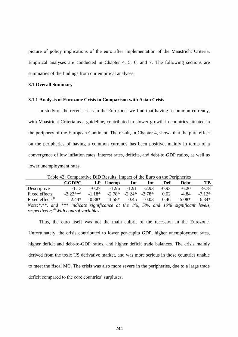
244

picture of policy implications of the euro after implementation of the Maastricht Criteria.

Empirical analyses are conducted in Chapter 4, 5, 6, and 7. The following sections are

summaries of the findings from our empirical analyses.

8.1 Overall Summary

8.1.1 Analysis of Eurozone Crisis in Comparison with Asian Crisis

In study of the recent crisis in the Eurozone, we find that having a common currency,

with Maastricht Criteria as a guideline, contributed to slower growth in countries situated in

the periphery of the European Continent. The result, in Chapter 4, shows that the pure effect

on the peripheries of having a common currency has been positive, mainly in terms of a

convergence of low inflation rates, interest rates, deficits, and debt-to-GDP ratios, as well as

lower unemployment rates.

Table 42. Comparative DiD Results: Impact of the Euro on the Peripheries

GGDPC LP Unemp Inf Int Def Debt TB

Descriptive -1.13 -0.27 -1.96 -1.91 -2.93 -0.93 -6.20 -9.78

Fixed effects -2.22*** -1.18* -2.78* -2.24* -2.78* 0.02 -4.84 -7.12*

Fixed effectsa)

-2.44* -0.88* -1.58* 0.45 -0.03 -0.46 -5.08* -6.34*

Note:*,**, and *** indicate significance at the 1%, 5%, and 10% significant levels,

respectively; a)

With control variables.

Thus, the euro itself was not the main culprit of the recession in the Eurozone.

Unfortunately, the crisis contributed to lower per-capita GDP, higher unemployment rates,

higher deficit and debt-to-GDP ratios, and higher deficit trade balances. The crisis mainly

derived from the toxic US derivative market, and was more serious in those countries unable

to meet the fiscal MC. The crisis was also more severe in the peripheries, due to a large trade

deficit compared to the core countries‘ surpluses.

245

The following table describes some similarities and differences between the ASEAN

economic crisis and the Eurozone crisis.

Table 43. Indicators of Crisis: Asian Crisis versus the Eurozone Crisis

Asian The Eurozone

High inflation Negative growth

Slow capital inflow and sudden capital

outflow

High deficit and debt-to-GDP

ratio

Property bubbles High unemployment

Private debt High trade deficit

Exchange rate collapse Property bubbles

8.1.2 Applying Maastricht Convergence Criteria in ASEAN

In the Chapter 4 analysis , we find that ASEAN has high convergence in terms of

interest rate, but in all other criteria, the level of convergence was lower than the Eurozone.

Comparing countries satisfying adapted MC, conditions were not much different in the EU

prior to adoption of the MT. Applying the MC in ASEAN, results show that Thailand met all

criteria, and most countries satisfied budget criteria, indicating fiscal sustainability in ASEAN

countries.

Regarding the EU, results showed that seventeen countries have joined the EMU, and it

continues expanding as more countries determine the benefits outweigh the costs of

membership. The level of nominal convergence based on the MC is very high (Cronbach‘s

coefficient above 0.9). Despite some limitations in facing the current crisis (Darvas, 2010),

the success of the euro‘s launch, its evolution to become a strong currency, and price stability

in the Eurozone were signs that the monetary and fiscal stability provided by the MC are

surely steps in the right direction.

246

Table 44. Comparing the Eurozone and ASEAN Related to MC Variables and Cronbach‘s

Coefficient


Eurozone 2.09 4.11 -2.66 69.92

Austria 1.82 4.13 -1.86 61.03

Belgium 2.01 4.15 -1.28 92.03

Finland 1.57 4.08 2.75 40.70

France 1.89 4.06 -3.73 65.75

Germany 1.64 3.93 -2.42 39.53

Ireland 2.52 4.30 -1.98 34.93

Italy 2.30 4.33 -3.40 98.32

Luxemburg 2.20 3.73 1.08 8.53

Netherlands 1.92 4.06 -1.37 43.50

Portugal 2.35 4.23 -2.35 67.67

Spain 2.93 4.13 -1.43 37.88

Cyprus 2.46 4.90 -2.54 62.55

Greece 3.22 4.47 -6.37 100.59

Malta 2.45 4.81 -4.48 66.04

Slovakia 4.15 4.85 -3.83 35.58

Slovenia 3.96 5.12 -1.44 26.45

ASEAN 8.75 6.48 -0.94 57.90

Indonesia 13.82 14.66 -0.96 53.77

Malaysia 2.43 3.74 -3.31 42.67

Philippines 5.62 6.58 -3.43 58.98

Singapore 1.20 1.21 5.64 91.86

Thailand 2.73 3.38 -1.79 48.93

Brunei 0.52 5.59 6.11 6.80

Cambodia 5.21 3.65 -1.64 35.33

Laos 25.77 8.17 -4.72 107.48

Myanmar 23.48 10.56 -2.05 85.84

Vietnam 6.75 7.25 -3.22 47.33

MC for the Eurozone 3.18 6.05 -3.00 60.00

MC for ASEAN 2.88 5.51 -3.00 60

Cronbach’s Coefficient (1983-1992, EMU-11) 0.92 0.84 0.57 0.90

Cronbach’s Coefficient (2002-2009, EMU-16) 0.94 0.95 0.93 0.85

Cronbach’s Coefficient ASEAN (1998-2009) 0.60 0.84 0.40 0.50 Source: Author’s calculation

247

Adapting the MC can impose stable macroeconomic performance, if ASEAN intents to

create deeper integration through a common currency. Some difficulty arises in

implementation, due to weaker institutions, huge differences in GDP per capita, financial

systems, and degree of market liberalization (Vanderon, 2005). In the current situation,

ASEAN should not rush into a deeper regional integration, as the EU did at stage I of the MT.

Previous studies‘ findings have some similarities and differences, as seen in following table.

Table 45. Comparing Previous Studies: Applying Maastricht Convergence Criteria Study Country (time period) Analysis Method Result

Green (1994)

ASEAN-4 (Indonesia,

Malaysia, Philippines,

Thailand)

EC-4 (France, Germany,

Italy, UK)

1970-1990

Crobach‘s

Coefficient

Convergence in nominal exchange rate, few convergence

trends for interest rates, more convergence in money

supply growth, 3 of ASEAN-4 appear to pass the kind of

tests for MC in EU.

Azali (2007)

ASEAN-5 1978-2004 The Bound Testing

Approach (ARDL)

Interest rate, inflation rate, and debt-ratio criteria satisfy

the Maastricht criteria, while exchange rate and surplus

criteria didn‘t comply. The findings showed ASEAN-5

countries have the potential to form a single currency.

Artus 1993 EC Countries The Maastricht

Criteria

Three countries pass the criteria. By the end of 1992,

much convergence progress had been achieved in a

majority of EC countries.

This study Comparing the Eurozone

and ASEAN countries

The Maastricht

Criteria and

Cronbach‘s

Coefficient

ASEAN has high convergence in term of interest rates,

but in all criteria, the level of convergence was lower than

the Eurozone. Comparing countries satisfying adapted

MC criteria, conditions were not much different than EU

countries prior to signing of the MT. Applying the MC in

ASEAN, results show that Thailand met all criteria, and

most countries satisfy budget criteria, indicating fiscal

sustainability in ASEAN countries.

8.1.3 Assessing Determinants of Macroeconomic Policy and Demographic Conditions on

Real Convergence and Growth

In the section above, we see ASEAN conditions regarding the Maastricht Criteria were

not much different than EU countries prior to signing of the MT; the level of convergence in

the Eurozone was very high, indicating that monetary and fiscal stability provided by the MC

is positive.

248

Other important aspects of this study are the analysis of regional integration of

membership and policy variables (mainly the MC) on growth and convergence. Studying

these issues can show whether these policies work effectively.

The issues analyzed in Chapter 5 have received little attention in previous studies. We

use various approaches to capture recent conditions of regional integration. The assumptions

used in Chapter 5 show whether regional economic integration membership, macroeconomic

policy variables, demographics, and crises contribute to growth and real convergence.

As also supported by DiD and decomposition computation, the results confirmed that

ASEAN member countries have no macroeconomic policy restrictions, and they performed

better in terms of income, productivity growth, and low levels of unemployment. However, in

terms of the business cycle, the Eurozone was more stable. The increase in GDP per hours

worked—wages—was responsible for the increase in productivity, especially in ASEAN,

which experienced high annual growth.

Based on regression results, convergence was found to be conditional rather than

unconditional, except in the case of unemployment and productivity in the Eurozone. The

ability to explain variations in dependent variables improved substantially when the condition

factor was included as the magnitude of convergence.

The inclusion of a dummy-membership variable showed mixed results. It was positive

in inducing the growth of per-capita GDP in both regions. It was also beneficial in terms of

productivity in ASEAN, but insignificant for the Eurozone. It was reduced ASEAN

unemployment growth, these figures increased in the Eurozone. Crisis was painful for both

regions, as suspected; however, it had no impact on unemployment.

249

Table 46. Comparing the Eurozone and ASEAN: Real Convergence Convergence in Income Productivity Unemployment

Eurozone ASEAN Eurozone ASEAN Eurozone ASEAN

Speed of Convergence

Unconditional Insig Insig –0.0201a Insig –0.1744a –0.4274a

With Dummy –0.2055a –0.0216b –0.0125b –0.0743a –0.1547a –0.4483a

Input Variables –0.2719a Insig –0.0214a –0.1385a –0.1258a –0.4450a

Maastricht Variables –0.3563a –0.0386b –0.0930a –0.1972a –0.1224a –0.5759a

Demographic Variables – – -0.0630a -0.3314a -0.2404a -0.6267a

Dummy Variables

Membership + + Insig + Insig –

Crisis – – – – + Insig

Input Variables

GK + + + + – –

GP – – Insig Insig

Openness Insig Insig + + – Insig

Gov – – Insig Insig + Insig


Inflation Insig Insig – + Insig Insig

Interest Rate Insig Insig Insig – + Insig

Exchange Rate Insig + Insig Insig Insig +

Deficit + Insig – + – Insig

Public Debt Insig Insig – Insig Insig +


Working-Age – + + Insig Insig Insig

Dependency Ratio – Insig Insig Insig Insig Insig

Density + Insig – – Insig +

Urban Insig Insig + Insig Insig +

Note: aSignificance in 1%, b in 5%, and c in 10%

The augmentation of input variables was essential for all equations. Positive growth in

the fixed capital formation aligned with the neoclassical assumption. The negative impact of

population growth on productivity and working age in per-capita income indicates that

increases in population diminish growth and induce responses in the form of technological

progress and capital accumulation. Unfortunately, population growth was found to have no

influence on unemployment volatility. Going deeper into the specific impact of

macroeconomic policy (i.e., those relating to the MC) on growth and real convergence, results

were mixed in different estimations. In the per-capita GDP equation, only deficit had a

positive influence on growth in the Eurozone, and depreciation had a positive impact on

growth in ASEAN.

250

The Eurozone‘s productivity estimation results indicated that inflation, deficits, and

public debt had negative effects on productivity growth, and on the control of convergence.

By contrast, in ASEAN, inflation and deficit each had a positive impact, and interest rates

discouraged growth.

Looking at unemployment convergence, the interest rate had a positive influence, and

deficits reduced unemployment. For ASEAN, the exchange rate and debt contributed

positively to unemployment growth. Due to limitations inherent in the panel estimation, care

should be taken with the interpretation of results, since country-specific effects should differ.

Therefore, country-specific investigations are needed to obtain a more robust interpretation.

Demographic variables were important to productivity in the Eurozone; however, among

variables included, only density had an impact on unemployment. For the MC variables,

Eurozone‘s policies designed to keep inflation low were relevant, since these variables had

the power to reduce productivity and increase unemployment.

For ASEAN, investment was a very important factor, inducing productivity and reducing

unemployment. Density had negative impact for productivity, and also increased

unemployment, especially for urban dwellers. In the case of ASEAN, public debt should be

lowered, to reduce the impact of negative productivity and an increase in unemployment.

While the MC as policy variables in both areas appears to play a major role in shaping

productivity and unemployment patterns, demographic conditions also matter (although in

unemployment equations, the individual effects are so determinant). The results of

demographic change in both regions supported the ―population neutralist‖ view, that

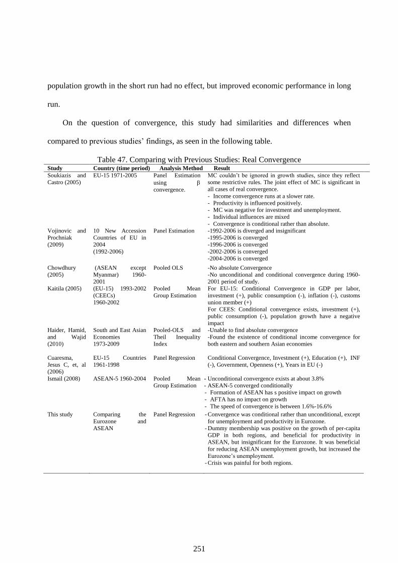
251

population growth in the short run had no effect, but improved economic performance in long

run.

On the question of convergence, this study had similarities and differences when

compared to previous studies‘ findings, as seen in the following table.

Table 47. Comparing with Previous Studies: Real Convergence Study Country (time period) Analysis Method Result

Soukiazis and

Castro (2005)

EU-15 1971-2005

Panel Estimation

using

convergence.

MC couldn‘t be ignored in growth studies, since they reflect

some restrictive rules. The joint effect of MC is significant in

all cases of real convergence.

- Income convergence runs at a slower rate.

- Productivity is influenced positively.

- MC was negative for investment and unemployment.

- Individual influences are mixed

- Convergence is conditional rather than absolute.

Vojinovic and

Prochniak

(2009)

10 New Accession

Countries of EU in

2004

(1992-2006)

Panel Estimation

-1992-2006 is diverged and insignificant

-1995-2006 is converged




Chowdhury

(2005)

(ASEAN except

Myanmar) 1960-

2001

Pooled OLS -No absolute Convergence

-No unconditional and conditional convergence during 1960-

2001 period of study.

Kaitila (2005)

(EU-15) 1993-2002

(CEECs)

1960-2002

Pooled Mean

Group Estimation

For EU-15: Conditional Convergence in GDP per labor,

investment (+), public consumption (-), inflation (-), customs

union member (+)

For CEES: Conditional convergence exists, investment (+),

public consumption (-), population growth have a negative

impact

Haider, Hamid,

and Wajid

(2010)

South and East Asian

Economies

1973-2009

Pooled-OLS and

Theil Inequality

Index

-Unable to find absolute convergence

-Found the existence of conditional income convergence for

both eastern and southern Asian economies

Cuaresma,

Jesus C, et, al

(2006)

EU-15 Countries

1961-1998

Panel Regression

Conditional Convergence, Investment (+), Education (+), INF

(-), Government, Openness (+), Years in EU (-)

Ismail (2008)

ASEAN-5 1960-2004

Pooled Mean

Group Estimation

- Unconditional convergence exists at about 3.8%

- ASEAN-5 converged conditionally

- Formation of ASEAN has s positive impact on growth

- AFTA has no impact on growth

- The speed of convergence is between 1.6%-16.6%

This study Comparing the

Eurozone and

ASEAN

Panel Regression - Convergence was conditional rather than unconditional, except

for unemployment and productivity in Eurozone.

- Dummy membership was positive on the growth of per-capita

GDP in both regions, and beneficial for productivity in

ASEAN, but insignificant for the Eurozone. It was beneficial

for reducing ASEAN unemployment growth, but increased the

Eurozone‘s unemployment.

- Crisis was painful for both regions.

252

8.1.4 Augmented Analysis of Economic Integration Impact on Trade

This paper investigates the impact of different levels of economic integration on bilateral

trade in these two regions, one with a common currency (the Eurozone), and the other

struggling as a free-trade area (ASEAN). Chapter 7 addresses this important issue.

We found that that the effects of deepening integration increased bilateral trade for all

Eurozone members, but insignificant for original members. Thus, widening membership

positively induced higher reciprocal trade. In ASEAN, the deepening impact of creating

AFTA generated positive results among ASEAN-6 countries, but not when CLMV joined.

Thus, inclusion of the CLMV in AFTA was negative. The financial crises reduced the

incentive to trade bilaterally in both the Eurozone and ASEAN.

Table 48. Comparing the Eurozone and ASEAN: Regional Integration on Trade

Eurozone ASEAN

Variable All Original All ASEAN-6

Euro Dummy + Insig - +

Crisis Dummy - - - -

DifInf Insig Insig Insig Insig

Difint + + Insig Insig

Difer Insig + Insig Insig

Difdef Insig Insig + Insig

Difdebt Insig Insig Insig -

G (Market Size) + + + +

S (Market Similarity) + + + +

R (Endowment) - Insig + Insig

D (Distance) - - - -

G*Euro - Insig + -

S*Euro - - - -

R*Euro + Insig Insig Insig

For the Eurozone, in regard to MC variables, divergence in interest rates creates an

incentive for higher bilateral trade. A similar effect was caused by divergence in nominal

exchange rates among original members, and a reassuring effect was created by convergence

253

in deficit-to-GDP ratio for original EU members, in export and import weight. This shows

that forcing convergence in the Maastricht criteria might not have an influence on higher

bilateral trade. For ASEAN, among variables associated with the MC, divergence in deficit

induced higher bilateral trade, and convergence in debt created the reassuring effect.

Related to H-O variables, the impact of market size, income similarity, and distance were

as hypotesised. Market size and income similarity were important factors for a higher flow of

bilateral trade, which indicated horizontal linkage creation, based predominantly on market

access and consumer income.

We found various results for factor endowment impact. Intra-trade industry increased

dramatically among all Eurozone countries, shown by the negative impact of factor

endowment on bilateral trade, but it was insignificant among original members, due to a

similar level of development among these nations. For ASEAN, differences in factor

endowment were determinant for higher bilateral trade when CLMV countries were included,

as shown by a positive result for factor endowment; however, among original members, the

impact was insignificant. This study found some similarities and differences with previous

studies‘ findings, as seen in following table.

254

Table 49. Comparing with Previous Studies: The Impact of Regional Integration on Trade Study Country (time period) Analysis Method Result

Frankel and

Rose (1998)

1959-1993

21 OECD Countries

Panel-OLS and IV

Distance related negatively to bilateral trade. Income,

common language, and regional trade among members

related positively to bilateral trade.

Countries with closer trade links tended to have more

tightly correlated business cycles.

Warin,

Wunnava and

Janicki (2009)

EU-15 members 1994-

2005

Panel Estimation H-O variables were robust for bilateral FDI, convergence

in debt was important, as were interaction variables.

Egger and

Pfaffermayr

(2013)

EU countries (1960-

2001)

ANCOVA

Regression Model

Substantial trade creation through the

formation/enlargement of EU.

Smaller trade creation effects of southern enlargement.

Significant intra-trade diversion of EU membership.

Core-periphery trade showed strong positive effects from

integration.

Yamarik and

Ghosh (2005)

186 Countries

1970, 1975, 1980, 1985,

1990, 1995

Cross Section Level of development, trade policy, linguistics, colonial

ties, geographic factors, relative population density,

common currency, and membership in trade

arrangements, are robust in a gravity equation.

Micco, Stein,

and Ordonez

(2003)

22 OECD Members

1992-2002

Panel Fixed Effect Common membership in the Eurozone contributed

positively on bilateral trade.

Sousa (2012) 203 Countries

1948-2009

PPML Technique

With globalization, currency unions become less and less

important for promoting trade.

Belke and

Spies (2008)

All OECD members

1991-2004

Panel Data

Poland, Latvia, and Lithuanian, all CEES, can expect

increases in the EMU-12 import share.

Berger and

Nitsch (2008)

22 OECD members

1948-2003

Panel OLS

estimation

A gradual increase of trade intensity between European

countries over time, due to trade integration and policy

changes.

Elliott and

Ikemoto (2004)

35 countries

1983-1999

Panel Estimation

Trade flows were not significantly affected in the years

immediately following the signing of AFTA, and

countries with outward-looking economies were

stimulated by AFTA.

Bun, Klaassen,

and Tan (2009)

11,178 country-pairs

1948-1997

Panel Estimation Negative impact of AFTA on trade.

Doanh and Heo

(2009)

Vietnam and Singapore

1990-2005

Panel Estimation AFTA, with other ASEAN countries, was negative for

Vietnam and positive for Singapore.

This Study The Eurozone and

ASEAN 1990-2009

Panel Estimation Deepening integration on bilateral trade was positive

among all Eurozone members, but insignificant among

original members. Membership expansion was positive,

inducing higher reciprocal trade. In ASEAN, the impact

of deepening the economic union, creating AFTA,

generated positive results only among ASEAN-6, not

when the CLMV joined the membership.

255

8.2 Overall Conclusions and Policy Recommendations

8.2.1 Findings

We can draw some findings from this research:

- The pure effect of a common currency on the EU peripheries has shown a positive

convergence of low inflation rates, interest rates, deficits, and debt-to-GDP ratios, as well

as lower unemployment rates. Unfortunately, the 2009 crisis contributed to lower per-

capita GDP, higher unemployment rates, higher deficit and debt-to-GDP ratios, and higher

deficit trade balances. The crisis mainly derived from the toxic US derivative market, and

was more serious in those countries unable to meet the fiscal MC.

- ASEAN has high convergence in terms of interest rates, but in all other criteria, the level

of convergence was lower than the Eurozone. Comparing countries satisfying the adapted

MC, conditions were not much different than EU countries prior to signing of the MT.

Our results show that Thailand met all criteria, and most countries satisfied budget

criteria, indicating fiscal sustainability in ASEAN countries.

- Convergence was found to be conditional rather than unconditional, except unemployment

and productivity in the Eurozone. The ability to explain variations in dependent variables

improved substantially when the condition factor was included as the magnitude of

convergence.

- The inclusion of a dummy-membership variable brought mixed results. It was positive for

growth of per-capita GDP in both regions. It was also beneficial in terms of productivity

256

in ASEAN, but insignificant for the Eurozone. It reduced ASEAN unemployment growth,

but increased it in the Eurozone.

- Macroeconomic policy variables relating to the MC, applied growth and real convergence,

showed mixed results in different estimates. In the per-capita GDP equation, only deficit

had a positive influence on growth in the Eurozone, and depreciation had a positive

impact on growth in ASEAN. The Eurozone‘s productivity estimates indicated that

inflation, deficit, and public debt had negative effects on productivity growth and on

control of convergence. By contrast, in ASEAN, inflation and deficit both had a positive

impact, and interest rates discouraged growth. Looking at unemployment convergence in

the EU, the interest rate had a positive influence and deficit reduced unemployment. For

ASEAN, the exchange rate and debt increased unemployment.

- The MC as policy variables appeared to play a major role in shaping productivity and

unemployment patterns. Demographic conditions were also important, although in the

unemployment equation, individual effects were not so determinant.

- We found that that deepening the union positively impacted bilateral trade among all

Eurozone countries, but was insignificant among original members. The euro‘s

membership expansion was positive in inducing reciprocal trade. In ASEAN, AFTA

generated positive results only among ASEAN-6, not when the CLMV joined the

membership. Thus, inclusion of the CLMV into AFTA was negative.

- Forcing convergence in variables associated with Maastricht criteria had little influence on

higher bilateral trade in both regions.

257

- Related with H-O variables, the impact of market size, income similarity, and distance

were as expected. Market size and income similarity were important factors for increased

bilateral trade, indicative of horizontal linkage, based predominantly on market access and

consumer income.

- Intra-trade industry was dramatic in all Eurozone countries, shown by the negative impact

of factor endowment on bilateral trade, but it was insignificant among original members,

due to similar levels of development. For ASEAN, differences in factor endowment were

determinant for higher bilateral trade when the CLMV countries were included, as shown

by a positive result for factor endowment.

8.2.2 Limitations

- Data availability constrained analysis.

- Data quality for ASEAN countries may not be as good as figures from the Eurozone. This

should be considered when evaluating the results.

- Although it fair to evaluate the euro a decade before and after as an empirical lesson for

ASEAN, analyzing a 20-year period might lead to less-robust results.

8.2.3 Policy Recommendations

- In the long-term, to preclude the systemic vulnerability associated with Minsky‘s cycle of

excessive risk in the Eurozone, the MC and SGP should be revised, thus creating more

unified fiscal policy in the Eurozone. The ECB should be entrusted with a larger budget,

so that it may act as a ―lender of last resort‖ and as a ―checks and balances‖ institution.

258

- Regardless of limitations, adapting the MC can be useful to create stable macroeconomic

performance. From the Maastricht Treaty, ASEAN can learn how to implement suitable

criteria for stronger guarantees of economic stability, and determine nominal convergence

as a necessary condition for adopting a common currency

- It was difficult to bring about a political union in the Eurozone with asymmetrical

monetary and fiscal-policy structures. Therefore, both the MC and SGP criteria were

needed, as were incentives for compliant member countries and clear sanctions for

noncompliance.

- To ensure a stronger Euro, a decade after its introduction, some criteria were set forth in

tandem with policy coordination—especially that which imposed price-stability tasks for

the ECB, pushed growth, and mitigated unemployment.

- In the Eurozone, greater economic integration was necessary to decrease trade disputes

and friction in the area, especially regarding trade imbalances among member countries.

- ASEAN needs to meet their commitment to lower tariffs based on the CEPT scheme, in

order to accelerate the realization of an ASEAN Economic Community by 2015.

- Although austerity compresses public expenditures and weakens private consumption, to

solve the current crisis in the Eurozone, it may steer the peripheries away from collapse in

the short term. The transfer of some funds from the surplus (core) countries, in order to

create job opportunities in the peripheries, will help reduce negative effects in the short

term.

259

REFERENCES

Afxentiou, P. (2000). Convergence, the Maastricht criteria, and their benefits. Winter/Spring

Journal, 7(1).

Afxentiou, P., & Serletis, A. (2000). Output growth and variability of export and import

growth: international evidence from granger causality tests. The Developing

Economies, 38(2), 141–163.

Agénor, P. R. (2003). Benefits and costs of international financial integration: theory and facts.

The World Economy, 26(28), 1089-1118.

Anand, M. R., Gupta, G. L., & Dash, R. (2012). The Euro Zone Crisis and its Dimensions and

Implications. Working Paper of Social Science.

Angresano, J. (2004). European Union integration lessons for ASEAN+3: the importance of

contextual specificity. Journal of Asian Economics, 14, 909-926.

Angrist, J. D. (1999). Empirical strategies in labor economics. In Handbook of labor

economicsElsevier.

Appleyard, D. R., Field, A. J., & Cobb, S. L. (2006). International economics trade, theory &

policy (5th ed.). McGraw-Hill.

Artus, J.R. (1993). Convergence - The Maastricht approach to economic and monetary union

(EMU) in Europe. Journal of Asian Economics, 4(2), 377-385.

Armstrong, H., & Taylor, J. (2000). Regional Economics and Policy (3rd ed.). Blackwell,

Oxford.

Avellaneda, S. D., & Hardiman, N. (2010). The European context of Ireland‘s economic crisis.

The Economic and Social Review, 41(4), 473-500.

260

Azali, M., Kelly, L. C., Shafinaz, A. N., & Wong, K. S. (2007). The ASEAN-5 future

currency: Maastricht criteria. Munich Personal RePEc Archive.

Baldwin, R. E., & Forslid, R. (2000). The core–periphery model and endogenous growth:

stabilizing and destabilizing integration. Economics, 67, 307-324.

Baldwin, R. E., & Wyplosz, C. (2012) The economics of European integration (4th ed.).

London/Boston: McGraw-Hill.

Barro, R. J., & Sala-i-Martin, X. (1992). Convergence. Journal of Political Economy, 100(2),

223–251.

Barro, R. J., & Sala-i-Martin, X. (2004). Economic growth (2nd ed.). Cambridge, MA: The

MIT Press.

Baskaran, T. (2009). Did the Maastricht Treaty matter for macroeconomic performance? A

difference-in-difference investigation. Kyklos, 62(3), 331–358.

Bassanini, A., & Scarpetta, S. (2001). The driving forces of economic growth: panel data

evidence for the OECD countries. OECD Economic Studies, 33.

Bassanini, A., & Duval, R. (2006). The determinants of unemployment across OECD

countries: reassessing the role of policies and institutions. OECD Economic Studies,

42.

Bayoumi, T., Eichengreen, B., & Mauro, P. (2000). On regional monetary arrangements for

ASEAN. Journal of the Japanese and International Economies, 14(2), 121-148.

Bernard, A. B., & Durlauf, S. N. (1996). Interpreting tests of the convergence

hypothesis. Journal of Econometrics, 71(1), 161-173.

261

Belke, A., & Spies, J. (2008). Enlarging the EMU to the east: what effects on trade?.

Empirica, 35, 369-89.

Bellofiore, R., Garibaldo, F., & Halevi, J. (2010). The global crisis and the crisis of European

neo-mercantilism. In Panitch Leo, Greg Albo, & Vivek Chibber (Hg.), Socialist

register 2011: The crisis this time (pp. 120-146). London, UK:

Bellofiore, R., & Halevi, J. (2011). A Minsky moment? The subprime crisis and the ‗new‘

capitalism. In Credit, money and macroeconomic policy, a post-Keynesian approach:

Edward Elgar Publishing Limited.

Benassy-Quere, A., & Boone, L. (2010). The euro zone crisis: debts, institutions and growth.

Le Cercle des Economistes. Retrieved from

http://www.lecercledeseconomistes.asso.fr/IMG/pdf/session_3_Benassy-

Boone_Texte_2_en_.pdf

Ben-David, D. (1998). Convergence clubs and subsistence economies. Journal of

Development Economics, 55(1), 155-171.

Bentolila, S., & Cahuc, P., (2010). Unemployment and temporary jobs in the crisis:

comparing France and Spain. Fedea Working Paper.

Biagi, F., & Lucifora, C. (2008). Demographic and education effects on unemployment in

Europe. Labour Economics, 15(5), 1076-1101.

Bijsterbosch, M., & Kolasa, M. (2010). FDI and productivity convergence in Central and

Eastern Europe: an industry-level investigation. Rev World Econ,145, 689–712.

Blanchard, O. J., & Katz, L. F. (1992). Regional evolutions. Brookings Papers on Economic

Activity, 1992(1), 1-75.

http://www.lecercledeseconomistes.asso.fr/IMG/pdf/session_3_Benassy-Boone_Texte_2_en_.pdf

http://www.lecercledeseconomistes.asso.fr/IMG/pdf/session_3_Benassy-Boone_Texte_2_en_.pdf

262

Blanchard, O. (2004). The economic future of Europe. Journal of Economic Perspectives,

18(4), 3–26.

Bloom, D. E., and Williamson, J. G., (1998), Demographic transitions and economic miracles

in emerging Asia. World Bank Economic Review, 12(3), 419–455.

Bloom, D. E., & Finlay, J.E. (2009). Demographic change and economic growth in Asia.

Asian Economic Policy Review, 4, 45-64.

Bloom, D. E., Canning, D., Hu, L., Liu, Y., Mahal, A., & Yip, W. (2010). The contribution

of population health and demographic change to economic growth in China and India.

Journal of Comparative Economics, 38, 17–32.

Brauninger, M., & Pannenberg, M. (2002). Unemployment and productivity growth: an

empirical analysis within an augmented Solow model. Economic Modeling, 19, 105–

120.

Buiter, W., Corsetti, G., & Roubini, N. (1993). Excessive deficits: sense and nonsense in the

Treaty of Maastricht. Economic Policy, April.

Bun, M. J. G., Franc, J. G., Klaassen, M., & Tan, R.G.K. (2009). Free trade areas and intra-

regional trade: the case of ASEAN. The Singapore Economic Review, 54(3), 319-334.

Carmines, E.G., & Zeller, R.A. (1979). Reliability and validity assessment. Thousand Oaks,

CA: Sage.

Casario, M., & Dadkhah, K.M. (1998). An evaluation of progress toward European Monetary

Union using fuzzy analysis. Journal of Policy Modeling, 20(6), 741–765.

Castro, V. (2010). The impact of the European Union fiscal rules on economic growth.

Journal of Macroeconomics. doi: 1016/j.macro.2010.09.003.

263

Cesaratto, S., & Stirati, A. (2010). Germany and the European and global crises. International

Journal of Political Economy, 39(4), 56-86.

Chan, K. S., Chao, C., & Chuo, W. L. (2002). Trade similarities and contagion among the

Asian crisis economies. Journal of Asian Economics, 13, 271-283.

Chowdhury, K. (2005). What‘s happening to per capita GDP in the ASEAN countries? An

analysis of convergence 1960–2001. Applied Econometrics and International

Development, 5(3).

Coale, A. J., & Hoover, E.M. (1958). Population growth and economic development in low-

income countries. Princeton, NJ: Princeton University Press.

Cortina, J.M. (1993). What is coefficient alpha? An examination of theory and applications.

Journal of Applied Psychology, 78, 98–104.

Cuvyers, L., Philippe D. L., & Verherstraeten, S. (2005). From AFTA towards an ASEAN

economic community and beyond. CAS Discussion Paper 46, Antwerp.

Darvas, Z. (2010). The case for reforming euro area entry criteria. Society and Economy,

32(2), 195-219.

De Grauwe, P. (1996). Monetary union and convergence economics. European Economic

Review, 40, 1091-1101.

De Grauwe, P. (2009). Economics of monetary union (8th ed.). Oxford, UK: Oxford

University Press.

De Grauwe, P., & Mongelli, F. P. (2011). Endogeneities of optimum currency areas. DJØF

Publishing.

264

De Nardis, S., & Vicarelli, C. (2003). Currency unions and trade: the special case of EMU.

World Review of Economics, 139, 625-649.

De la Fuente, A. (2002). On the sources of convergence: a close look at the Spanish regions.

European Economic Review, 46(3), 569-599.

De Rosa, D. A. (1998). Regional integration arrangements: static economic theory,

quantitative finding, and policy guideline. World Bank, Development Research Group,

No. 2007.

Doanh, N. K., & Heo, Y. (2009). AFTA and trade diversion: an empirical study for Vietnam

and Singapore. International Area Review, 12(1).

Egger, P. H., & Pfaffermayr, M. (2013). The pure effects of European integration on intra-EU

core and periphery trade. The World Economy.

Eichengreen, B. (1992). Should the Maastricht Treaty be saved? Princeton Study in

International Finance, 74.

Eichengreen, B. (1993). European monetary unification. Journal of Economic

Literature, 31(3), 1321-1357.

Elliott, R. J. R., & Ikemoto, K. (2004). AFTA and the Asian crisis: help or hindrance to

ASEAN intra-regional trade? Asian Economic Journal, 18(1).

Escot, L., & Galindo, M. A. (2000). International capital flows and convergence in the

neoclassical growth model. International Advances in Economic Research, 6(3), 451-

460.

Feyrer, J. (2007). Demographic and productivity. The Review of Economics and Statistics,

89(1), 100-109.

265

Frankel, J. A., & Rose, A. K. (1996). The endogeneity of the optimum currency area criteria.

NBER Working Paper, 5700.

Frankel, J. A., & Rose, A. K. (2002). An estimate of the effect of common currencies on trade

and income. The Quarterly Journal of Economics.

Furceri, D., & Zdzienicka, A. (2012). How costly are debt crises? Journal of International

Money and Finance, 31(4), 726-742.

Glick, R., & Rose, A. K. (2002). Does a currency union affect trade? The time series evidence.

European Economic Review, 46, 1125-1151.

Green, D.J. (1994). Convergence and cohesion within the ASEAN-4. Journal of Asian

Economics, 5(1), 119-144.

Gros, D., & Alcidi, C. (2011). Adjustment difficulties and debt overhangs in the Eurozone

periphery. CEPS Working Document, 347.

Guldager, P. (1997). Convergence of the EU member states towards the EMU requirements,

1986 to 1993. European Journal of Political Economy, 13, 247-259.

Hapsari, I. M., & Mangunsong, C. (2006). Determinants of AFTA members‘ trade flows and

potential for trade diversion. Asia-Pacific Research and Training Network on Trade

Working Paper Series, 21.

Heckscher, E. F. (1935). Mercantilism (Vols. 1-2). London, UK: Allend & Unwin.

Hein, E., & Truger, A. (2005). European Monetary Union: nominal convergence, real

divergence and slow growth. Journal Structural Change and Economic Dynamics, 16,

7–13.

266

Hein, E., & Truger, A. (2009). The crisis: how to fight (or not to fight) a slowdown.

Challenge, 52(3), 52-75.

Helpman, E., & Krugman, P. (1985). Market Structure and Foreign Trade. Cambridge, MA:

MIT Press.

Helpman, E. (1987). Imperfect competition and international trade: evidence from fourteen

industrial countries. Journal of the Japanese and International Economies, 1, 62-81.

Hill, H., & Menon, J. (2010). ASEAN economic integration: features, fulfillments, failures

and the future. ADB Working Paper Series on Regional Economic Integration, 69.

Hume, D. (1955). Of the balance of trade. In Eugene Rotwein (Ed.), David Hume: Writings

on Economics. Madison, WI: University of Wisconsin Press.

Irvin, G. (2005). The implosion of the brussels economic consensus. International Centre for

Economic Research, Working Paper, 11.

Irwin, D. A. (1966). Against the Tide: an Intellectual History of Free Trade. Princeton, NJ:

Princeton University Press.

Ismail, N. W. (2008). Growth and convergence in ASEAN: a dynamic panel approach.

International Journal of Economics and Management, 2(1), 127-140.

Johnson, D., & Turner, C. (2009). International Business: Themes and Issues in the Modern

Global Economy. Taylor & Francis.

Jovanovic, M.N. (2006). The Economics of International Integration. MA: Edward Elgar

Publishing.

Kaitila, V. (2005). Integration and conditional convergence in the enlarged EU area, ENEPRI

Working Paper, 31.

267

Kaminsky, G. L., & Reinhart, C. M. (1998). Financial crises in Asia and Latin America: then

and now. The American Economic Review, 88(2), 444-448.

Kawai, M. (2005). East Asian economic regionalism: progress and challenges. Journal of

Asian Economics,16(1), 29-55.

Kelly, A. C., & Schmidt, R. M. (1995). Aggregate population and economic growth

correlations: the role of the components of demographic change. Demography, 32(4),

543–555.

Kenen, P. (2003). Making the case for the euro. The International Economy, Winter, 51-54.

Kho, B., & Stulz, R. M. (2000). Banks, the IMF, and the Asian crisis. Pacific-Basin Finance

Journal, 8, 177-216.

Kim, Y. (2001). The Asian crisis, private sector saving, and policy implications. Journal of

Asian Economics, 12, 331-351.

Klaasen, F. (2004). Why is it so difficult to find an effect of exchange rate risk on trade?

Journal of International Money and Finance, 23(5), 817-839.

Kumakura, M. (2006). Trade and business cycle co-movements in Asia-Pacific. Journal of

Asian Economics, 17(4), 622-645.

Krugman, P. R. (1979). A model of innovation, technology transfer, and the world

distribution of income. Journal of Political Economy, 87(2), 253-266.

Krugman, P. R. (1981). Intra-industry specialization and the gains from trade. The Journal of

Political Economy, 89(5), 959-973.

Krugman, P. R. (1991). Geography and trade. Cambridge, MA: MIT press.

Krugman, P. R. (1992). Second thoughts on EMU. Japan and the World Economy, 4, 187-200.

http://www.sciencedirect.com/science/journal/10490078

http://www.sciencedirect.com/science/journal/10490078

268

Kaltenbrunner, A., Lambrinidis, G., Lapavitsas, C., Lindo, D., Meadway, J., Michell, J.,

Painceira, J.P., . . . Teles, N. (2010). The Eurozone between austerity and default.

Research on Money and Finance. RM Occasional Report.

Kaltenbrunner, A., Lapavitsas, C., Michell, J., Painceira, J.P., Pires, E., Powell, J., Stenfors,

A., & Teles, N. (2010). Eurozone crisis: beggar thyself and thy neighbor. Journal of

Balkan and Near Eastern Studies, 12(4), 321-373.

Lee, R., & Mason, A. (2010). Fertility, human capital, and economic growth over the

demographic transition. Eur J Population, 26, 159-182.

Linder, S. B. (1961). An essay on trade and transformation. John Willey and Sons.

Ljungqvist, L., & Sargent, T. J. (2008). Two questions about European unemployment.

Econometrica, 76(1), 1–29.

Lombard, M. (2000). Restrictive macroeconomic policies and unemployment in the European

Union. Review of Political Economy, 12(3), 317–332.

Madhur, S. (2002). Costs and benefits of a common currency for ASEAN. Asian

Development Bank (ADB) ERD Working Paper, 12.

Mahmood, T., & Sial, M. H. (2012). The relative effectiveness of monetary and fiscal policies

in economic growth: a case study of Pakistan. Asian Economic and Financial Review,

1(4), 236-244.

Marelly, E., & Signorelly, M. (2010). Institutional, nominal and real convergence in Europe.

Banks and Bank System, 5(2).

Markusen, J. R., & Venables, A. (2000). The theory of endowment, intra-industry and multi-

national trade. Journal of International Economics, 52, 209-234.

269

McKinnon, R. I. (2004). Optimum currency areas and key currencies: Mundell I versus

Mundell II. JCMS: Journal of Common Market Studies, 42(4), 689-715.

Meyer, B. D. (1994). Natural and quasi-experiment in economics. NBER Technical Working

Paper, 170.

Mico, A., Stein, E., & Ordonez, G. (2003). The currency union effect on trade: early evidence

from EMU. Economic Policy, 315-356.

Minsky, H. P. (1977). The financial instability hypothesis: an interpretation of Keynes and an

alternative to ‗standard‘ theory. Challenge, 20(1), 20-28.

Mishkin, F. S. (1999). Lessons from the Asia crisis. Journal of International Money and

Finance, 18, 709–723.

Miyakoshi, T. (2000). The causes of the Asian currency crisis: empirical observations. Japan

and the World Economy, 12, 243-253.

Mongelli, F. P. (2005). What is European economic and monetary union telling us about the

properties of optimum currency areas? Journal of Common Market Studies, 43(3),

607–635.

Mundell, R. A. (1961). A theory of optimum currency areas. American Economic Review, 51,

657–665.

Mundell, R. (1973). Uncommon arguments for common currencies. In H. G. Johnson & A. K.

Swoboda (Eds.), The economics of common currencies (pp. 114-132). London, UK:

Allen & Unwin.

270

Mutaqin, Z., & Ichihashi, M. (2012). Assessing determinants of macroeconomic policy on

real convergence and growth: a comparative study of the Eurozone and ASEAN.

Asian Economic and Financial Review, 2(2), 301-324.

Mutaqin, Z., & Ichihashi, M. (2012). Productivity and unemployment convergence in the

Eurozone and ASEAN: a comparative study based on demographic and Maastricht

criteria roles. International Journal of Trade Economics and Finance, 3(6), 450-457.

Mutaqin, Z., & Ichihashi, M. (2013). Applying Maastricht convergence criteria in ASEAN.,

Under Consideration to The IUP Journal of Applied Economics.

Mutaqin, Z., & Ichihashi, M. (2013). Tracking the Eurozone crisis in peripheral countries,

Under Consideration to Journal of Economic Issues.

Niebuhr, A., & Stiller, S. (2002). Integration effects in border regions : a survey of economic

theory and empirical studies. HWWA Discussion Paper, 179.

Obstfeld, M., & Rogoff, K. S. (2009). Global imbalances and the financial crisis: products of

common causes. Centre for Economic Policy Research.

Onwuka, K. O., Baharumshah, A. Z., & Habibullah, M. S. (2006). Trading system and

convergence hypothesis: evidence from ASEAN-5 countries. International Journal of

Finance and Economics, 5, 14-28.

Palley, T. I. (2011). A theory of Minsky super-cycles and financial crisis. Contributions to

Political Economy, 30(1), 31-46.

Papaioannou, G. (2010). Can the stability and growth pact criteria lead to sustainable growth?

International Research Journal of Finance and Economics, 5.

271

Pelkmans, J. (2001). European integration-methods and economic analysis. (2nd ed.). Harlow,

UK: Financial Times Prentice Hall.

Perez-Caldentey, E., Vernengo, M. (2012). The euro imbalances and financial deregulation: a

post-Keynesian interpretation of the European debt crisis. Levy Economic Institute

Working Paper, 702.

Persson, J. (2002). Demographics, human capital, and economic growth: a study of us states

1930-2000. FIEF Working Paper.

Posner, M. V. (1961). International trade and technical change. Oxford Economic Papers New

Series, 13, 323-341.

Quah, D. (1996). Empirics for Economic Growth and Convergence. European Economic

Review, 40, 1353-1375.

Radelet, S., & Sachs, J. (2000). The onset of the East Asian financial crisis. In Currency crisis

book (pp. 105-162). Chicago, IL: University of Chicago Press.

Reinhart, C., & Rogoff. K. (2010). Debt and growth revisited. Munich Personal RePEc,

Archive No. 24376.

Rose, A. K. (2000). One money, one market: the effect of common currencies on trade.

Economic Policy.

Ruffin, R. J. (1999). The nature and significance of intra-industry trade. Federal Reserve

Bank of Dallas Economic and Financial Review, 2-9.

Sareal, M. (1995). Demographic dynamics and the empirics of economic growth. IMF Staff

Papers, 398-410.

272

Sarno, L., & Taylor, M. P. (1999). Moral hazard, asset price bubbles, capital flows, and the

East Asian crisis: the first tests. Journal of International Money and Finance, 18, 637-

657.

Savona, P., & Viviani, C. (2003). The impact of the stability and growth pact on real

economic growth: automatic mechanisms or policy discretion? Review of Economic

Conditions in Italy, 2, 263–279.

Schiavo, S. (2008). Financial integration, GDP correlation and the endogeneity of optimum

currency areas. Economica, 75, 168-189.

Schuknecht, L., Moutot, P., Rother, P., & Stark, J. (2011). The stability and growth pact:

crisis and reform. European Central Bank, 129.

Shimizu, K. (2010). ASEAN economic integration in the world economy—toward the

ASEAN economic community. Economic Journal of Hokkaido University, 39, 77–88.

Solow, R. M. (1956). A contribution to the theory of economic growth. Quarterly Journal of

Economics, 70, 65–94.

Soukiazis, E., & Castro, V. (2005). How the Maastricht criteria and stability and growth pact

affected real convergence in the European Union: a panel data analysis. Journal of

Policy Modeling, 27, 385–399.

Sousa, J. (2012). The currency union effect on trade is decreasing over time. Economics

Letters, 117, 917-920.

Splimbergo, A., Londono, J. L., & Szekely, M. (1999). Income, distribution, factor

endowments, and trade openness. Journal of Development Economics, 59(1), 77-101.

273

Stiglitz, J. E. (2000). Capital market liberalization, economic growth, and instability. World

Development, 28(6), 1075-1086.

Tavlas, G. S. (1994). The theory of monetary integration. Open Economies Review, 5(2), 211-

230.

Tinberge, J. (1962). Shaping the world economy: Suggestions for an international economic

policy. New York, NY: The Twentieth Century Fund.

Tse, J. (2001). Minsky‘s financial instability hypothesis. Oeconomicus, 4, 77-81.

Tyrowicz, J., & Wojcik, P. (2010). Active labor market policies and unemployment

convergence in transition. Review of Economic Analysis, 2, 46–72.

Vanderon, P. (2005). Regional economic integration in South East Asia. Asian Economic

Journal, 3, 517–535.

Vernon, R. (1966). International investment and international trade in the product cycle.

Quarterly Journal of Economics, 80(2), 190-207.

Viner, J. (1950). The customs union issue. New York, NY: Carnegie Endowment for

International Peace.

Vines, D. (2011). Recasting the macroeconomic policymaking system in Europe. Foundation

Universitaire in Brussels. Retrieved from www.pegged.cepr.org.

Vojinovic, B., & Prochniak, M. (2009). Divergence period in the European convergence

process. Transition Study Review, 15, 685-700.

Wade, R. (1998). The Asian debt-and-development crisis of 1997: causes and consequences.

World Development, 26(8), 1535-1553.

274

Warin, T., Wunnava, P. V., & Janicki, H. P. (2009). Testing Mundell‘s institution of

endogenous OCA theory. Review of International Economics, 17(1), 74-86.

Wattanapruttipaisan, T. (2006). A brief on ASEAN economic integration. BEIF Studies Unit,

7.

Whyte, P. (2010, October). Why Germany is not a model for the Eurozone. Retrieved from the

Centre for European Reform Web site: www.cer.org.uk/sites/default/file

Wyplosz, C. (2010). The Eurozone in the current crisis. ADBI Working Paper, 207.

Xu, Z.L., Ward, B.D., & Gan, C. (2007). A single currency for ASEAN-5: an empirical study

of economic convergence and symmetry. In Kim S., & Mckenzie, M.D., (Eds.), Asia-

Pacific Financial Markets: Integration, Innovation and Challenges, International (pp.

117-139). Finance Review LOCATION: Emerald Group Publishing Limited. 8

Yamarik, S., & Ghosh, S. (2005). A sensitivity analysis of the gravity model. The

International Trade Journal, 19(1), 83-126.

Žďárek, V., & Šindel, J. (2009). Selected issues relating to real and nominal convergence on

new EU member states. Monetary Policy, Trade and Convergence: The Case of

Transition Economies, 2, 163.

ASEAN Secretary. (DATE) Retrieved from http://www.aseansec.org

International Monetary Fund. (2012). World economic outlook databases. Retrieved from

http://www.imf.org/external/ns/cs.aspx?id=28

Organisation for Economic Co-operation and Development. (2012). OECD statistics database.

Retrieved from http://stats.oecd.org/


http://www.imf.org/external/ns/cs.aspx?id=28

http://stats.oecd.org/

275

The Conference Board Total Economy Database™. (2011). Retrieved from


The European Central Bank. (2011). Retrieved from http://www.ecb.int

The United Nation Statistic Division. (2011). National accounts main aggregate database.

Retrieved from http://unstats.un.org/unsd/snaama/Introduction.asp

The World Bank. (2012). World development indicators. Retrieved from

http://data.worldbank.org/data-catalog/world-development-indicators


http://www.ecb.int/

http://unstats.un.org/unsd/snaama/Introduction.asp

http://data.worldbank.org/data-catalog/world-development-indicators

Doctoral Dissertation



ZAENAL MUTAQIN

Graduate School for International Development and Cooperation

Hiroshima University

September 2013



D102422

ZAENAL MUTAQIN

A Dissertation Submitted to

the Graduate School for International Development and Cooperation

of Hiroshima University in Partial Fulfillment

of the Requirement for the Degree of

Doctor of Philosophy

September 2013

Documents

Doctoral Dissertation Comparative Analysis of …...Doctoral Dissertation Comparative Analysis of Convergence on Regional Economic Integration: The Eurozone and ASEAN ZAENAL MUTAQIN