No. 1 October 4, 2010

Do Vouchers and Tax Credits Increase Private School Regulation?

Andrew J. Coulson

Cato Institute 1000 Massachusetts Avenue, N.W.

Washington, D.C. 20001

The Cato Working Papers are intended to circulate research in progress for comment and discussion. Available at www.cato.org/workingpapers.

CATO Working Paper

Do Vouchers and Tax Credits Increase Private School Regulation?

A Statistical Analysis

By Andrew J. Coulson1

October 4, 2010

Abstract School voucher and education tax credit programs have proliferated in the United States

over the past two decades. Advocates have argued that they will enable families to become active

consumers in a free and competitive education marketplace, but some fear that these programs

may in fact bring with them a heavy regulatory burden that could stifle market forces. Until now,

there has been no systematic, empirical investigation of that concern. The present paper aims to

shed light on the issue by quantifying the regulations imposed on private schools both within and

outside school choice programs, and then analyzing them with descriptive statistics and

regression analyses. The results are tested for robustness to alternative ways of quantifying

private school regulation, and to alternative regression models, and the question of causality is

addressed. The study concludes that vouchers, but not tax credits, impose a substantial and

statistically significant additional regulatory burden on participating private schools.

1 Andrew J. Coulson directs the Cato Institute's Center for Educational Freedom and is author of the Journal of

School Choice study: "Comparing Public, Private, and Market Schools." He blogs at www.Cato-at-Liberty.org.

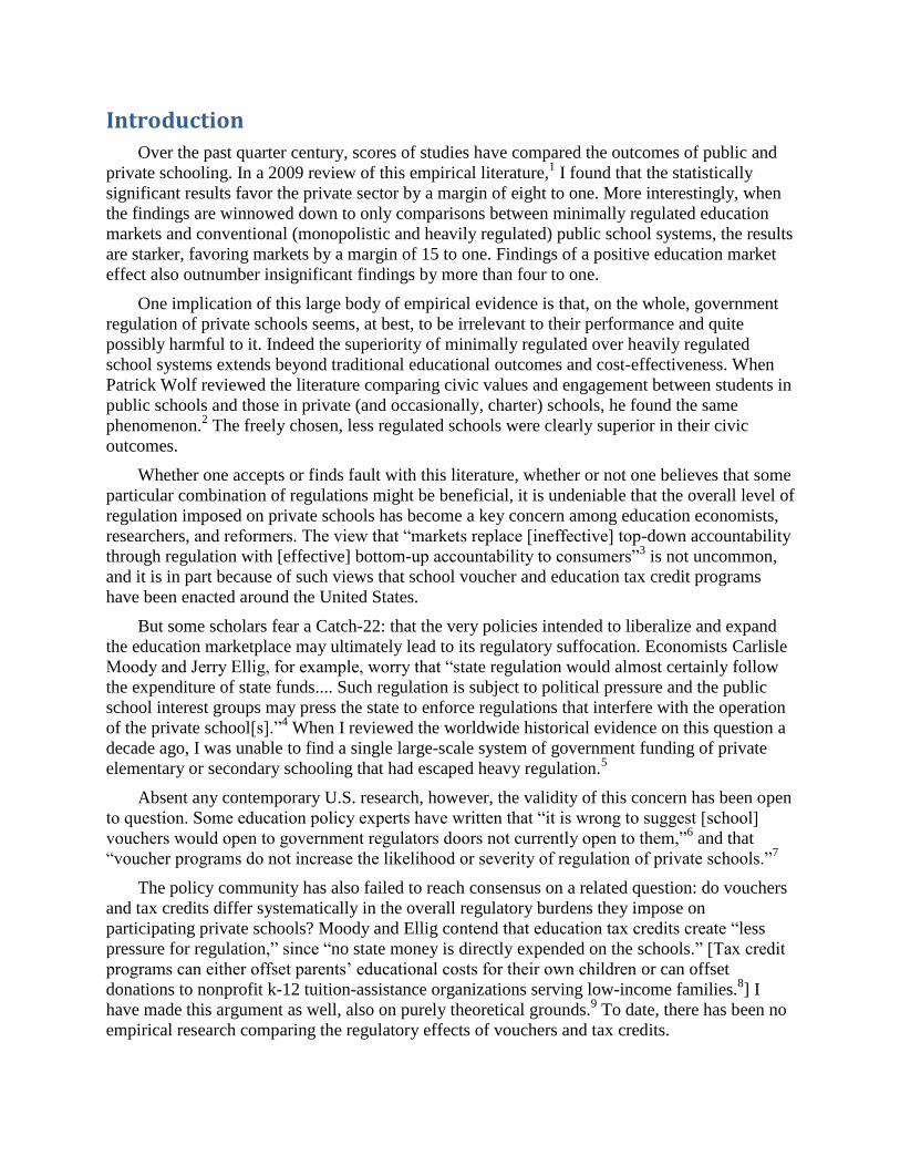
Introduction

Over the past quarter century, scores of studies have compared the outcomes of public and

private schooling. In a 2009 review of this empirical literature,1 I found that the statistically

significant results favor the private sector by a margin of eight to one. More interestingly, when

the findings are winnowed down to only comparisons between minimally regulated education

markets and conventional (monopolistic and heavily regulated) public school systems, the results

are starker, favoring markets by a margin of 15 to one. Findings of a positive education market

effect also outnumber insignificant findings by more than four to one.

One implication of this large body of empirical evidence is that, on the whole, government

regulation of private schools seems, at best, to be irrelevant to their performance and quite

possibly harmful to it. Indeed the superiority of minimally regulated over heavily regulated

school systems extends beyond traditional educational outcomes and cost-effectiveness. When

Patrick Wolf reviewed the literature comparing civic values and engagement between students in

public schools and those in private (and occasionally, charter) schools, he found the same

phenomenon.2 The freely chosen, less regulated schools were clearly superior in their civic

outcomes.

Whether one accepts or finds fault with this literature, whether or not one believes that some

particular combination of regulations might be beneficial, it is undeniable that the overall level of

regulation imposed on private schools has become a key concern among education economists,

researchers, and reformers. The view that ―markets replace [ineffective] top-down accountability

through regulation with [effective] bottom-up accountability to consumers‖3 is not uncommon,

and it is in part because of such views that school voucher and education tax credit programs

have been enacted around the United States.

But some scholars fear a Catch-22: that the very policies intended to liberalize and expand

the education marketplace may ultimately lead to its regulatory suffocation. Economists Carlisle

Moody and Jerry Ellig, for example, worry that ―state regulation would almost certainly follow

the expenditure of state funds.... Such regulation is subject to political pressure and the public

school interest groups may press the state to enforce regulations that interfere with the operation

of the private school[s].‖4 When I reviewed the worldwide historical evidence on this question a

decade ago, I was unable to find a single large-scale system of government funding of private

elementary or secondary schooling that had escaped heavy regulation.5

Absent any contemporary U.S. research, however, the validity of this concern has been open

to question. Some education policy experts have written that ―it is wrong to suggest [school]

vouchers would open to government regulators doors not currently open to them,‖6 and that

―voucher programs do not increase the likelihood or severity of regulation of private schools.‖7

The policy community has also failed to reach consensus on a related question: do vouchers

and tax credits differ systematically in the overall regulatory burdens they impose on

participating private schools? Moody and Ellig contend that education tax credits create ―less

pressure for regulation,‖ since ―no state money is directly expended on the schools.‖ [Tax credit

programs can either offset parents’ educational costs for their own children or can offset

donations to nonprofit k-12 tuition-assistance organizations serving low-income families.8] I

have made this argument as well, also on purely theoretical grounds.9 To date, there has been no

empirical research comparing the regulatory effects of vouchers and tax credits.

Not surprisingly, the tax credits vs. vouchers question is also contentious. Disputing the

view just presented, Australian economist John Humphreys wrote in 2002 that ―it seems unlikely

that there would be any stricter standards under a voucher system than a tax credit system, or

under the current system. Indeed, in the United States, restrictions on the Milwaukee voucher

programme have actually decreased and attempts to increase them again have been defeated.‖10

Though Humphreys’ latter statement was true at the time he made it, it should be noted that a set

of additional regulations was imposed on the Milwaukee program in 2009.11

Clearly, there is a need for a systematic empirical investigation of these questions. While the

amount of data available for study is regrettably small, that cannot be helped. Policy decisions

are being made regarding private school choice programs every year, and many interested parties

wish to know whether or not they will lead to regulatory proliferation and whether one policy

would bring with it more regulation than another. Our only alternatives are to continue to fumble

in the dark on these questions, or to inform ourselves as best we can with the available data. The

present study attempts to do the latter.

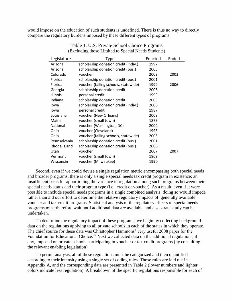
Data and Methods As of late September 2010, 20 voucher and tax credit programs have been enacted in 15

states and the District of Columbia to defray private school tuition for a general student

population (see Table 1). These programs are the focus of the present analysis. Excluded from

this study are education tax deductions and tax credits limited to non-tuition expenses. This is to

avoid biasing the results in favor of conventional tax credits, since it is reasonable to expect that

deductions and non-tuition credits will precipitate less regulation than full-fledged tax credits

that defray tuition costs at private schools. Since there are only two such programs (both from

Minnesota and both lightly regulated) they cannot be analyzed separately.12

Also excluded from this analysis are tax credit and voucher programs exclusively serving

special needs populations, such as disabled students. Due to the highly varied circumstances of

special needs children, it is effectively impossible to develop a single curriculum or testing

regime that could serve them all, and hence there is substantially less political pressure to impose

curriculum and testing regulations on schools serving them.

For example, Florida’s tax credit program requires participating schools to administer a

norm-referenced test of their choosing, but only to their non-disabled students. Disabled students

are exempt from the requirement.13

The Florida Opportunity Scholarships voucher program

required participating students to take the same test as public school students, but the public

school assessment system includes alternative testing arrangements or the waiving of tests for

disabled children.14

Similarly, Florida’s McKay voucher program exclusively targeted at

disabled students is exempt from any testing requirement. Clearly, serving special needs students

has a distinct causal effect on regulation, independent of program type.

This puts special needs programs into a separate category from programs serving a broader

student population, and at present there are too few special needs programs to allow for separate

statistical analysis. Neither is it possible to combine special needs programs with the more

general programs into a single analysis, for two reasons. First, doing so would require

comparable data for the regulatory burdens imposed by both types of programs. But because

special needs programs do not serve non-special-needs students, the level of regulation that they

would impose on the education of such students is undefined. There is thus no way to directly

compare the regulatory burdens imposed by these different types of programs.

Table 1. U.S. Private School Choice Programs (Excluding those Limited to Special Needs Students)

Legislature Type Enacted Ended Arizona scholarship donation credit (indiv.) 1997 Arizona scholarship donation credit (bus.) 2005 Colorado voucher 2003 2003 Florida scholarship donation credit (bus.) 2001 Florida voucher (failing schools, statewide) 1999 2006 Georgia scholarship donation credit 2008 Illinois personal credit 1999 Indiana scholarship donation credit 2009 Iowa scholarship donation credit (indiv.) 2006 Iowa personal credit 1987 Louisiana voucher (New Orleans) 2008 Maine voucher (small town) 1873 National voucher (Washington, DC) 2004 Ohio voucher (Cleveland) 1995 Ohio voucher (failing schools, statewide) 2005 Pennsylvania scholarship donation credit (bus.) 2001 Rhode Island scholarship donation credit (bus.) 2006 Utah voucher 2007 2007 Vermont voucher (small town) 1869 Wisconsin voucher (Milwaukee) 1990

Second, even if we could devise a single regulation metric encompassing both special needs

and broader programs, there is only a single special needs tax credit program in existence; an

insufficient basis for apportioning the variance in regulation among such programs between their

special needs status and their program type (i.e., credit or voucher). As a result, even if it were

possible to include special needs programs in a single combined analysis, doing so would impede

rather than aid our effort to determine the relative regulatory impacts of generally available

voucher and tax credit programs. Statistical analysis of the regulatory effects of special needs

programs must therefore wait until additional data are available and a separate study can be

undertaken.

To determine the regulatory impact of these programs, we begin by collecting background

data on the regulations applying to all private schools in each of the states in which they operate.

The chief source for these data was Christopher Hammons’ very useful 2008 paper for the

Foundation for Educational Choice.15

Next we collected data on the additional regulations, if

any, imposed on private schools participating in voucher or tax credit programs (by consulting

the relevant enabling legislation).

To permit analysis, all of these regulations must be categorized and then quantified

according to their intensity using a single set of coding rules. Those rules are laid out in

Appendix A, and the corresponding data are presented in Table 2 (lower numbers and lighter

colors indicate less regulation). A breakdown of the specific regulations responsible for each of

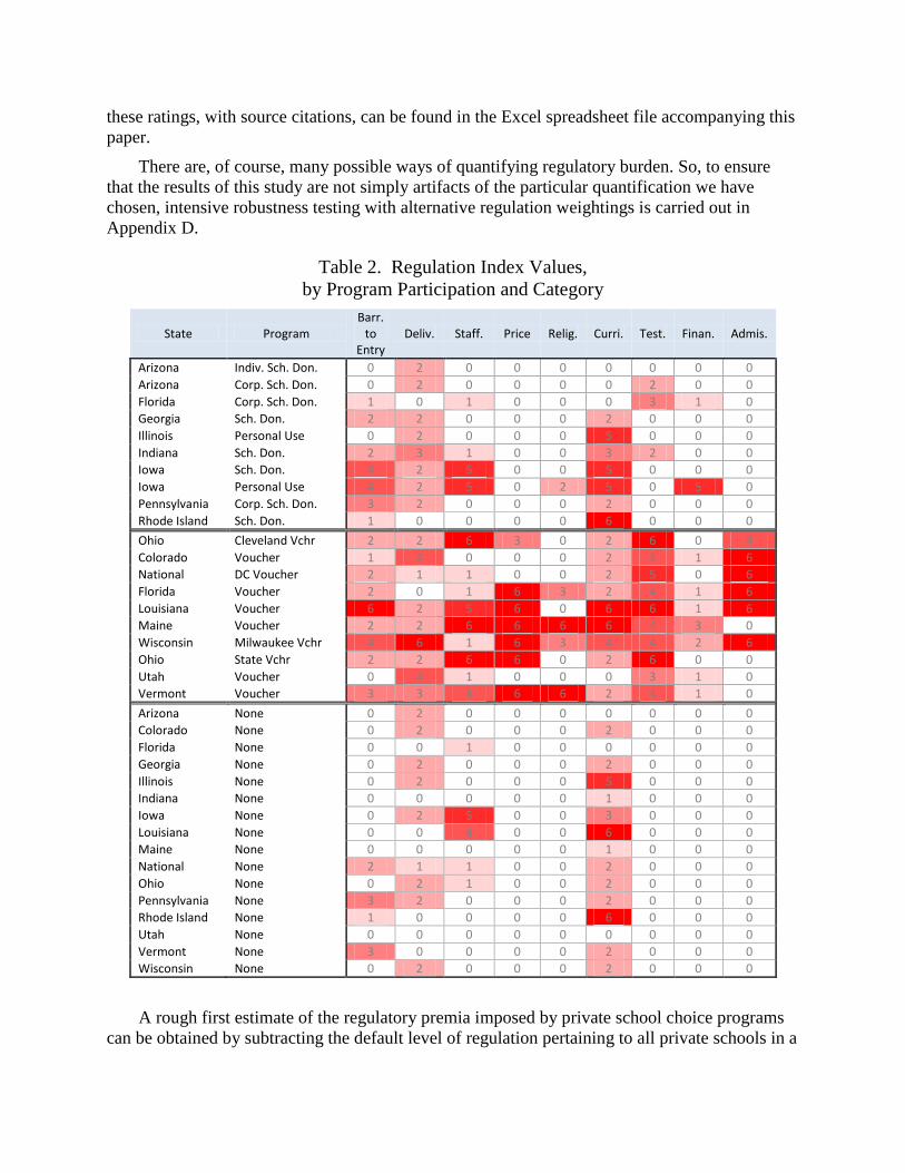
these ratings, with source citations, can be found in the Excel spreadsheet file accompanying this

paper.

There are, of course, many possible ways of quantifying regulatory burden. So, to ensure

that the results of this study are not simply artifacts of the particular quantification we have

chosen, intensive robustness testing with alternative regulation weightings is carried out in

Appendix D.

Table 2. Regulation Index Values,

by Program Participation and Category

State Program Barr.

to Entry

Deliv. Staff. Price Relig. Curri. Test. Finan. Admis.

Arizona Indiv. Sch. Don. 0 2 0 0 0 0 0 0 0

Arizona Corp. Sch. Don. 0 2 0 0 0 0 2 0 0

Florida Corp. Sch. Don. 1 0 1 0 0 0 3 1 0

Georgia Sch. Don. 2 2 0 0 0 2 0 0 0

Illinois Personal Use 0 2 0 0 0 5 0 0 0

Indiana Sch. Don. 2 3 1 0 0 3 2 0 0

Iowa Sch. Don. 4 2 5 0 0 5 0 0 0

Iowa Personal Use 4 2 5 0 2 5 0 5 0

Pennsylvania Corp. Sch. Don. 3 2 0 0 0 2 0 0 0

Rhode Island Sch. Don. 1 0 0 0 0 6 0 0 0

Ohio Cleveland Vchr 2 2 6 3 0 2 6 0 4

Colorado Voucher 1 4 0 0 0 2 4 1 6

National DC Voucher 2 1 1 0 0 2 5 0 6

Florida Voucher 2 0 1 6 3 2 4 1 6

Louisiana Voucher 6 2 5 6 0 6 6 1 6

Maine Voucher 2 2 6 6 6 6 4 3 0

Wisconsin Milwaukee Vchr 4 6 1 6 3 4 4 2 6

Ohio State Vchr 2 2 6 6 0 2 6 0 0

Utah Voucher 0 4 1 0 0 0 3 1 0

Vermont Voucher 3 3 4 6 6 2 4 1 0

Arizona None 0 2 0 0 0 0 0 0 0

Colorado None 0 2 0 0 0 2 0 0 0

Florida None 0 0 1 0 0 0 0 0 0

Georgia None 0 2 0 0 0 2 0 0 0

Illinois None 0 2 0 0 0 5 0 0 0

Indiana None 0 0 0 0 0 1 0 0 0

Iowa None 0 2 5 0 0 3 0 0 0

Louisiana None 0 0 4 0 0 6 0 0 0

Maine None 0 0 0 0 0 1 0 0 0

National None 2 1 1 0 0 2 0 0 0

Ohio None 0 2 1 0 0 2 0 0 0

Pennsylvania None 3 2 0 0 0 2 0 0 0

Rhode Island None 1 0 0 0 0 6 0 0 0

Utah None 0 0 0 0 0 0 0 0 0

Vermont None 3 0 0 0 0 2 0 0 0

Wisconsin None 0 2 0 0 0 2 0 0 0

A rough first estimate of the regulatory premia imposed by private school choice programs

can be obtained by subtracting the default level of regulation pertaining to all private schools in a

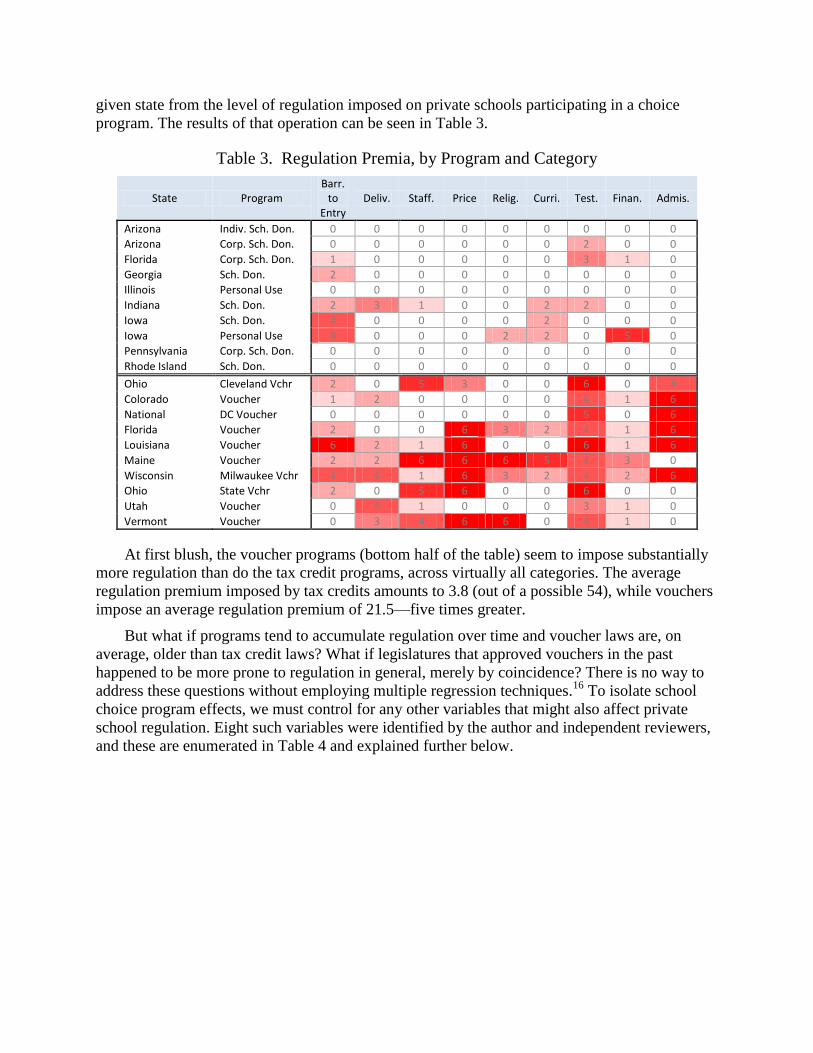
given state from the level of regulation imposed on private schools participating in a choice

program. The results of that operation can be seen in Table 3.

Table 3. Regulation Premia, by Program and Category

State Program Barr.

to Entry

Deliv. Staff. Price Relig. Curri. Test. Finan. Admis.

Arizona Indiv. Sch. Don. 0 0 0 0 0 0 0 0 0

Arizona Corp. Sch. Don. 0 0 0 0 0 0 2 0 0

Florida Corp. Sch. Don. 1 0 0 0 0 0 3 1 0

Georgia Sch. Don. 2 0 0 0 0 0 0 0 0

Illinois Personal Use 0 0 0 0 0 0 0 0 0

Indiana Sch. Don. 2 3 1 0 0 2 2 0 0

Iowa Sch. Don. 4 0 0 0 0 2 0 0 0

Iowa Personal Use 4 0 0 0 2 2 0 5 0

Pennsylvania Corp. Sch. Don. 0 0 0 0 0 0 0 0 0

Rhode Island Sch. Don. 0 0 0 0 0 0 0 0 0

Ohio Cleveland Vchr 2 0 5 3 0 0 6 0 4

Colorado Voucher 1 2 0 0 0 0 4 1 6

National DC Voucher 0 0 0 0 0 0 5 0 6

Florida Voucher 2 0 0 6 3 2 4 1 6

Louisiana Voucher 6 2 1 6 0 0 6 1 6

Maine Voucher 2 2 6 6 6 5 4 3 0

Wisconsin Milwaukee Vchr 4 4 1 6 3 2 4 2 6

Ohio State Vchr 2 0 5 6 0 0 6 0 0

Utah Voucher 0 4 1 0 0 0 3 1 0

Vermont Voucher 0 3 4 6 6 0 4 1 0

At first blush, the voucher programs (bottom half of the table) seem to impose substantially

more regulation than do the tax credit programs, across virtually all categories. The average

regulation premium imposed by tax credits amounts to 3.8 (out of a possible 54), while vouchers

impose an average regulation premium of 21.5—five times greater.

But what if programs tend to accumulate regulation over time and voucher laws are, on

average, older than tax credit laws? What if legislatures that approved vouchers in the past

happened to be more prone to regulation in general, merely by coincidence? There is no way to

address these questions without employing multiple regression techniques.16

To isolate school

choice program effects, we must control for any other variables that might also affect private

school regulation. Eight such variables were identified by the author and independent reviewers,

and these are enumerated in Table 4 and explained further below.

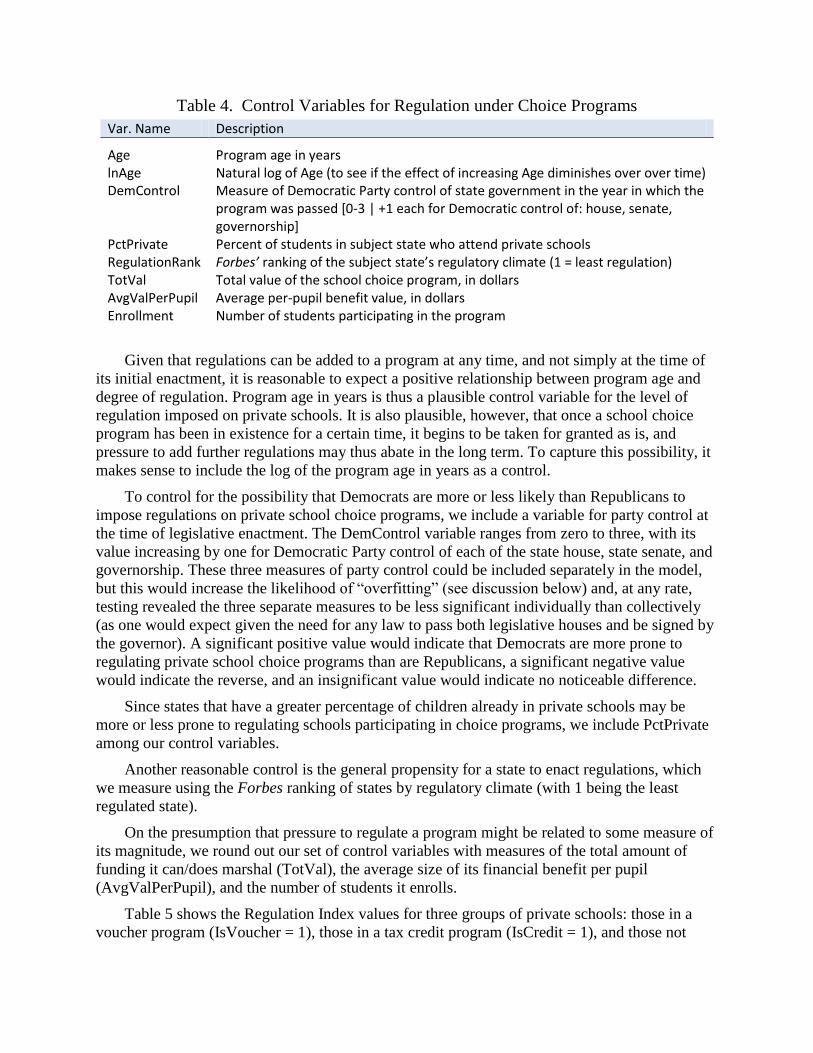
Table 4. Control Variables for Regulation under Choice Programs

Var. Name Description

Age Program age in years lnAge Natural log of Age (to see if the effect of increasing Age diminishes over over time) DemControl Measure of Democratic Party control of state government in the year in which the

program was passed [0-3 | +1 each for Democratic control of: house, senate, governorship]

PctPrivate Percent of students in subject state who attend private schools RegulationRank Forbes’ ranking of the subject state’s regulatory climate (1 = least regulation) TotVal Total value of the school choice program, in dollars AvgValPerPupil Average per-pupil benefit value, in dollars Enrollment Number of students participating in the program

Given that regulations can be added to a program at any time, and not simply at the time of

its initial enactment, it is reasonable to expect a positive relationship between program age and

degree of regulation. Program age in years is thus a plausible control variable for the level of

regulation imposed on private schools. It is also plausible, however, that once a school choice

program has been in existence for a certain time, it begins to be taken for granted as is, and

pressure to add further regulations may thus abate in the long term. To capture this possibility, it

makes sense to include the log of the program age in years as a control.

To control for the possibility that Democrats are more or less likely than Republicans to

impose regulations on private school choice programs, we include a variable for party control at

the time of legislative enactment. The DemControl variable ranges from zero to three, with its

value increasing by one for Democratic Party control of each of the state house, state senate, and

governorship. These three measures of party control could be included separately in the model,

but this would increase the likelihood of ―overfitting‖ (see discussion below) and, at any rate,

testing revealed the three separate measures to be less significant individually than collectively

(as one would expect given the need for any law to pass both legislative houses and be signed by

the governor). A significant positive value would indicate that Democrats are more prone to

regulating private school choice programs than are Republicans, a significant negative value

would indicate the reverse, and an insignificant value would indicate no noticeable difference.

Since states that have a greater percentage of children already in private schools may be

more or less prone to regulating schools participating in choice programs, we include PctPrivate

among our control variables.

Another reasonable control is the general propensity for a state to enact regulations, which

we measure using the Forbes ranking of states by regulatory climate (with 1 being the least

regulated state).

On the presumption that pressure to regulate a program might be related to some measure of

its magnitude, we round out our set of control variables with measures of the total amount of

funding it can/does marshal (TotVal), the average size of its financial benefit per pupil

(AvgValPerPupil), and the number of students it enrolls.

Table 5 shows the Regulation Index values for three groups of private schools: those in a

voucher program (IsVoucher = 1), those in a tax credit program (IsCredit = 1), and those not

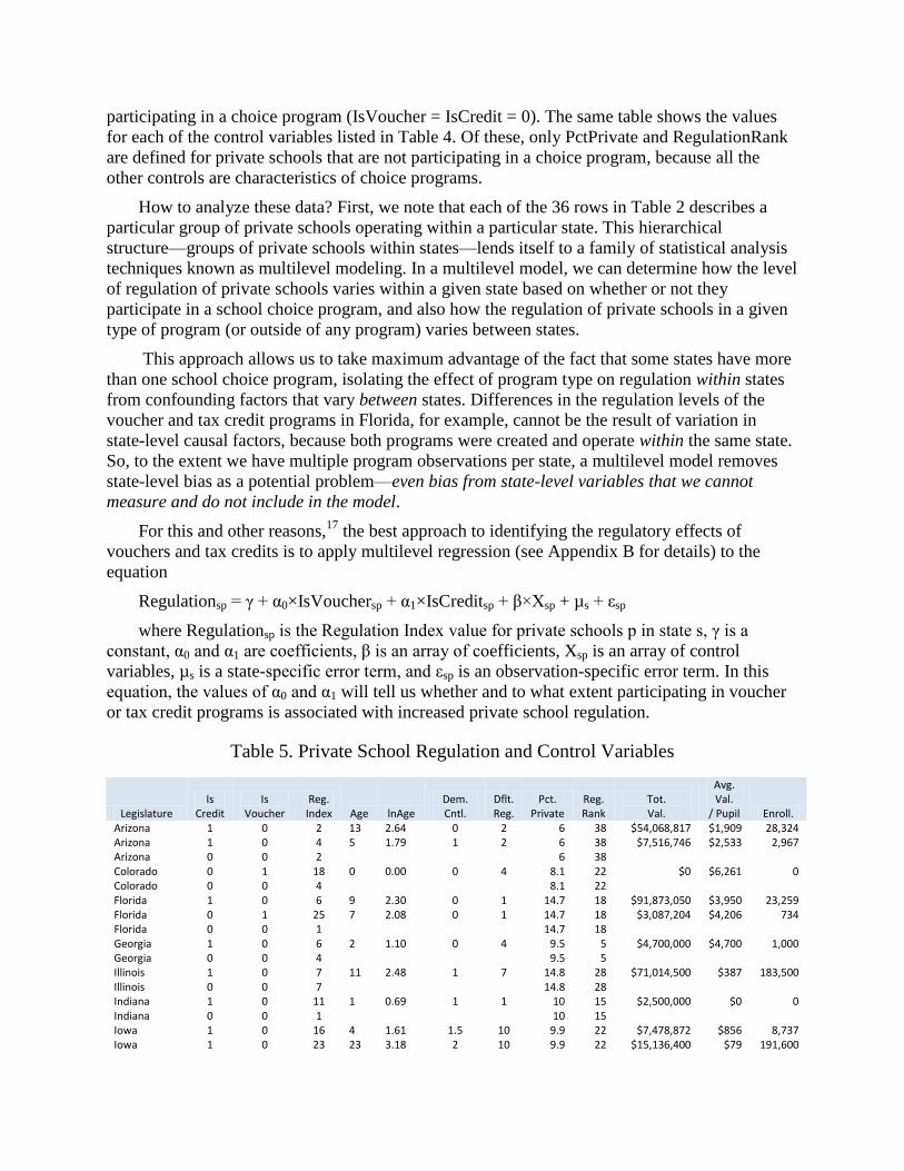
participating in a choice program (IsVoucher = IsCredit = 0). The same table shows the values

for each of the control variables listed in Table 4. Of these, only PctPrivate and RegulationRank

are defined for private schools that are not participating in a choice program, because all the

other controls are characteristics of choice programs.

How to analyze these data? First, we note that each of the 36 rows in Table 2 describes a

particular group of private schools operating within a particular state. This hierarchical

structure—groups of private schools within states—lends itself to a family of statistical analysis

techniques known as multilevel modeling. In a multilevel model, we can determine how the level

of regulation of private schools varies within a given state based on whether or not they

participate in a school choice program, and also how the regulation of private schools in a given

type of program (or outside of any program) varies between states.

This approach allows us to take maximum advantage of the fact that some states have more

than one school choice program, isolating the effect of program type on regulation within states

from confounding factors that vary between states. Differences in the regulation levels of the

voucher and tax credit programs in Florida, for example, cannot be the result of variation in

state-level causal factors, because both programs were created and operate within the same state.

So, to the extent we have multiple program observations per state, a multilevel model removes

state-level bias as a potential problem—even bias from state-level variables that we cannot

measure and do not include in the model.

For this and other reasons,17

the best approach to identifying the regulatory effects of

vouchers and tax credits is to apply multilevel regression (see Appendix B for details) to the

equation

Regulationsp = γ + α0×IsVouchersp + α1×IsCreditsp + β×Xsp + µs + εsp

where Regulationsp is the Regulation Index value for private schools p in state s, γ is a

constant, α0 and α1 are coefficients, β is an array of coefficients, Xsp is an array of control

variables, µs is a state-specific error term, and εsp is an observation-specific error term. In this

equation, the values of α0 and α1 will tell us whether and to what extent participating in voucher

or tax credit programs is associated with increased private school regulation.

Table 5. Private School Regulation and Control Variables

Legislature Is

Credit Is

Voucher Reg.

Index Age lnAge Dem. Cntl.

Dflt. Reg.

Pct. Private

Reg. Rank

Tot. Val.

Avg. Val.

/ Pupil Enroll. Arizona 1 0 2 13 2.64 0 2 6 38 $54,068,817 $1,909 28,324 Arizona 1 0 4 5 1.79 1 2 6 38 $7,516,746 $2,533 2,967 Arizona 0 0 2 6 38 Colorado 0 1 18 0 0.00 0 4 8.1 22 $0 $6,261 0 Colorado 0 0 4 8.1 22 Florida 1 0 6 9 2.30 0 1 14.7 18 $91,873,050 $3,950 23,259 Florida 0 1 25 7 2.08 0 1 14.7 18 $3,087,204 $4,206 734 Florida 0 0 1 14.7 18 Georgia 1 0 6 2 1.10 0 4 9.5 5 $4,700,000 $4,700 1,000 Georgia 0 0 4 9.5 5 Illinois 1 0 7 11 2.48 1 7 14.8 28 $71,014,500 $387 183,500 Illinois 0 0 7 14.8 28 Indiana 1 0 11 1 0.69 1 1 10 15 $2,500,000 $0 0 Indiana 0 0 1 10 15 Iowa 1 0 16 4 1.61 1.5 10 9.9 22 $7,478,872 $856 8,737 Iowa 1 0 23 23 3.18 2 10 9.9 22 $15,136,400 $79 191,600

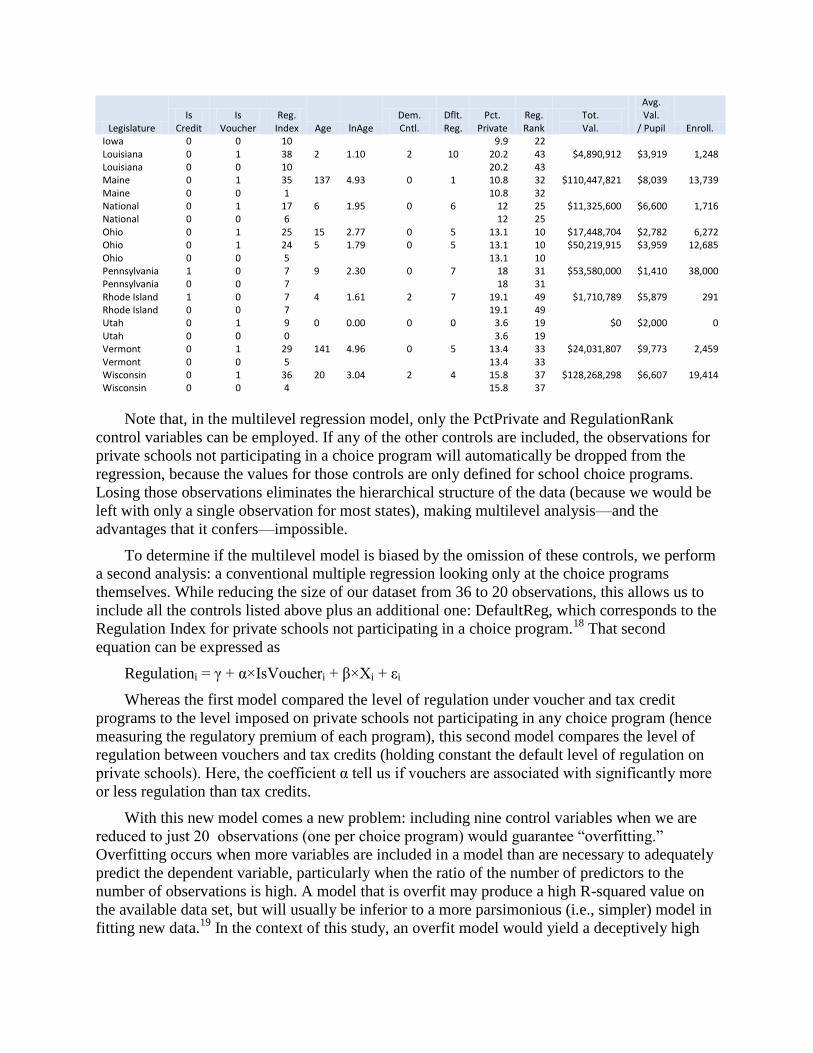
Legislature Is

Credit Is

Voucher Reg.

Index Age lnAge Dem. Cntl.

Dflt. Reg.

Pct. Private

Reg. Rank

Tot. Val.

Avg. Val.

/ Pupil Enroll. Iowa 0 0 10 9.9 22 Louisiana 0 1 38 2 1.10 2 10 20.2 43 $4,890,912 $3,919 1,248 Louisiana 0 0 10 20.2 43 Maine 0 1 35 137 4.93 0 1 10.8 32 $110,447,821 $8,039 13,739 Maine 0 0 1 10.8 32 National 0 1 17 6 1.95 0 6 12 25 $11,325,600 $6,600 1,716 National 0 0 6 12 25 Ohio 0 1 25 15 2.77 0 5 13.1 10 $17,448,704 $2,782 6,272 Ohio 0 1 24 5 1.79 0 5 13.1 10 $50,219,915 $3,959 12,685 Ohio 0 0 5 13.1 10 Pennsylvania 1 0 7 9 2.30 0 7 18 31 $53,580,000 $1,410 38,000 Pennsylvania 0 0 7 18 31 Rhode Island 1 0 7 4 1.61 2 7 19.1 49 $1,710,789 $5,879 291 Rhode Island 0 0 7 19.1 49 Utah 0 1 9 0 0.00 0 0 3.6 19 $0 $2,000 0 Utah 0 0 0 3.6 19 Vermont 0 1 29 141 4.96 0 5 13.4 33 $24,031,807 $9,773 2,459 Vermont 0 0 5 13.4 33 Wisconsin 0 1 36 20 3.04 2 4 15.8 37 $128,268,298 $6,607 19,414 Wisconsin 0 0 4 15.8 37

Note that, in the multilevel regression model, only the PctPrivate and RegulationRank

control variables can be employed. If any of the other controls are included, the observations for

private schools not participating in a choice program will automatically be dropped from the

regression, because the values for those controls are only defined for school choice programs.

Losing those observations eliminates the hierarchical structure of the data (because we would be

left with only a single observation for most states), making multilevel analysis—and the

advantages that it confers—impossible.

To determine if the multilevel model is biased by the omission of these controls, we perform

a second analysis: a conventional multiple regression looking only at the choice programs

themselves. While reducing the size of our dataset from 36 to 20 observations, this allows us to

include all the controls listed above plus an additional one: DefaultReg, which corresponds to the

Regulation Index for private schools not participating in a choice program.18

That second

equation can be expressed as

Regulationi = γ + α×IsVoucheri + β×Xi + εi

Whereas the first model compared the level of regulation under voucher and tax credit

programs to the level imposed on private schools not participating in any choice program (hence

measuring the regulatory premium of each program), this second model compares the level of

regulation between vouchers and tax credits (holding constant the default level of regulation on

private schools). Here, the coefficient α tell us if vouchers are associated with significantly more

or less regulation than tax credits.

With this new model comes a new problem: including nine control variables when we are

reduced to just 20 observations (one per choice program) would guarantee ―overfitting.‖

Overfitting occurs when more variables are included in a model than are necessary to adequately

predict the dependent variable, particularly when the ratio of the number of predictors to the

number of observations is high. A model that is overfit may produce a high R-squared value on

the available data set, but will usually be inferior to a more parsimonious (i.e., simpler) model in

fitting new data.19

In the context of this study, an overfit model would yield a deceptively high

R-squared while reducing our confidence that it would accurately predict the level of regulation

imposed by future school choice programs.

To minimize this problem, we must identify the smallest subset of the theoretically plausible

predictor variables that adequately explains the level of regulation of private school choice

programs, weeding out those predictors that add little or no explanatory power to the model. The

most thorough way to do this is to evaluate every possible regression equation made up of five or

fewer predictors, chosen from our set of ten20

(a process that can be easily automated using

modern statistical analysis software). From the resulting 637 possible models, we identify the

one that has the best combination of explanatory power and parsimony, as measured by a statistic

known as Mallow’s Cp.21

To validate the model thus identified, we also calculate two alternative measures of power

and parsimony for the top three models in the Mallow’s ranking just obtained. Both alternative

measures, Akaike’s Information Criterion (AIC) and the Bayesian Information Criterion (BIC),22

agree with the Mallow’s ranking that the optimal model is comprised of just four variables:

IsVoucher, lnAge, DemControl, and RegulationRank—the other theoretically plausible control

variables listed in Table 4 turn out to be poor predictors of private school regulation. Our

parsimonious OLS regression equation is thus:

Regulationi = γ + α×IsVoucheri + β0×lnAgei + β1×DemControli + β2×RegulationRanki + εi

This model was tested to determine if it satisfies the assumptions of OLS, and the results of

those tests are provided in Appendix C. The only OLS assumption that is clearly violated is the

independence of the observations from one another. As already noted, several states have more

than one school choice program and there may be state-specific factors affecting regulation that

we have not observed and hence cannot control for with a simple OLS approach. Failing to

control for the violation of this OLS assumption could lead to incorrect standard errors and

confidence intervals for our explanatory variables, undermining tests of statistical significance.

To deal with this issue, we produce Huber White robust standard errors, clustering our

observations by state (Stata command ―cluster(StateID)‖).23

Causality Even if the coefficients on either of our key explanatory variables (IsVoucher and IsCredit)

turn out to be statistically significant, we will be left with the question: is the relationship

between program type and degree of private school regulation causal? In theory, there could be

an unmeasured independent variable that both causes states to prefer one type of program over

the other and causes them to increase regulation of private schools participating in school choice

programs. If so, the IsVoucher or IsCredit variables would be said to be ―endogenous,‖ and their

coefficients would no longer measure their own unique causal impact on private school

regulation.

As already noted in the preceding section, our use of multi-level modeling minimizes the

possibility of a confounding state-level variable that simultaneously determines both the type of

program selected and the degree of regulation it imposes. That is because several states have

more than one school choice program. The relationship between the level of private school

regulation that these programs impose cannot be affected by variation in an unmeasured state-

level variable, because the given programs are within the same state. Florida, as noted earlier,

has enacted both a voucher and a tax credit program and imposed very different levels of

regulation on them. That is inconsistent with the endogeneity theory, which posits that some

unmeasured variable simultaneously determines both propensity to regulate choice programs and

the type of choice program enacted.

In principle, we could also test for endogeneity by using a two-stage-least-squares model

with instrumental variables, but this method is discouraged for small sample sizes such as we are

faced with here.24

Moreover, even if we had more observations, no obvious instrumental

variables for program type present themselves, making this test impossible. Fortunately, there is

considerable additional evidence that endogeneity is unlikely to be a problem.

First, consider that a state’s general proclivity to regulate is captured by the RegulationRank

variable, and this variable is controlled for in the OLS model. Furthermore, RegulationRank’s

correlation with IsVoucher is very small and negative (-0.07). So a state’s general proclivity to

regulate is associated with neither higher regulation of school choice programs nor the selection

of one program type over another. It thus cannot be a source of endogeneity.

Second, consider that DefaultReg (the default level of regulation imposed on all private

schools in a given state) is not a statistically significant predictor of choice program regulation

(and it was dropped from our parsimonious OLS regression for that reason). Furthermore, its

level of correlation with IsVoucher is also small and negative (-0.16). So even the specific

proclivity to regulate private schools is insignificantly (and negatively) correlated with choosing

vouchers over credits, and is irrelevant to how heavily regulated a choice program is. So it, too,

cannot be a source of endogeneity.

Third, Illinois came very close to passing a voucher bill in May 2010 that would have

imposed some extra regulations on private schools, but that state already has a tax credit program

that does not impose any additional regulations. As with the Florida example given above, this is

inconsistent with the endogeneity of IsVoucher or IsCredit.

Fourth, Arizona enacted two special needs voucher programs within a few years of enacting

its tax credit programs. This suggests that the state shows no particular favoritism for one type of

program over another, contrary to what we would expect under the endogeneity hypothesis.

Fifth, the DemControl variable is a significant predictor of higher program regulation, but is

only very weakly (and negatively) correlated with IsVoucher (-0.26). This is inconsistent with

the endogeneity hypothesis—even more so given the results reported in the following section.

Together, these facts and the resistance of our multilevel model to state-level omitted

variable bias militate against the likelihood of endogeneity of IsVoucher and IsCredit. To the

extent that IsVoucher or IsCredit is a significant predictor of private school regulatory burden, it

therefore seems reasonable to conclude that the relationship is causal, though we cannot remove

all uncertainty on this point.

Findings and Discussion The detailed results of the multilevel and robust OLS regression analyses appear in

appendices B and C, respectively, and are summarized in Table 5. Each row reports the

coefficient value for the given variable and, in parentheses, its standard error.

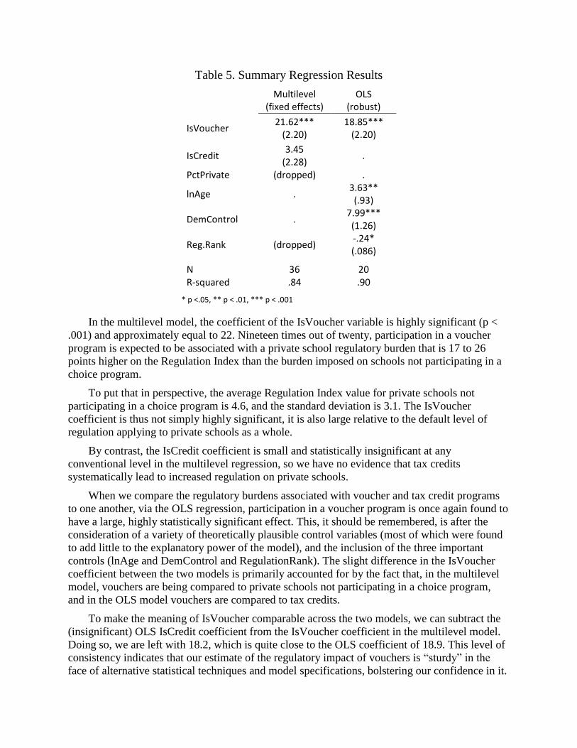
Table 5. Summary Regression Results

Multilevel

(fixed effects) OLS

(robust)

IsVoucher 21.62***

(2.20) 18.85***

(2.20)

IsCredit 3.45

(2.28) .

PctPrivate (dropped) .

lnAge . 3.63** (.93)

DemControl . 7.99*** (1.26)

Reg.Rank (dropped) -.24* (.086)

N 36 20 R-squared .84 .90

* p <.05, ** p < .01, *** p < .001

In the multilevel model, the coefficient of the IsVoucher variable is highly significant (p <

.001) and approximately equal to 22. Nineteen times out of twenty, participation in a voucher

program is expected to be associated with a private school regulatory burden that is 17 to 26

points higher on the Regulation Index than the burden imposed on schools not participating in a

choice program.

To put that in perspective, the average Regulation Index value for private schools not

participating in a choice program is 4.6, and the standard deviation is 3.1. The IsVoucher

coefficient is thus not simply highly significant, it is also large relative to the default level of

regulation applying to private schools as a whole.

By contrast, the IsCredit coefficient is small and statistically insignificant at any

conventional level in the multilevel regression, so we have no evidence that tax credits

systematically lead to increased regulation on private schools.

When we compare the regulatory burdens associated with voucher and tax credit programs

to one another, via the OLS regression, participation in a voucher program is once again found to

have a large, highly statistically significant effect. This, it should be remembered, is after the

consideration of a variety of theoretically plausible control variables (most of which were found

to add little to the explanatory power of the model), and the inclusion of the three important

controls (lnAge and DemControl and RegulationRank). The slight difference in the IsVoucher

coefficient between the two models is primarily accounted for by the fact that, in the multilevel

model, vouchers are being compared to private schools not participating in a choice program,

and in the OLS model vouchers are compared to tax credits.

To make the meaning of IsVoucher comparable across the two models, we can subtract the

(insignificant) OLS IsCredit coefficient from the IsVoucher coefficient in the multilevel model.

Doing so, we are left with 18.2, which is quite close to the OLS coefficient of 18.9. This level of

consistency indicates that our estimate of the regulatory impact of vouchers is ―sturdy‖ in the

face of alternative statistical techniques and model specifications, bolstering our confidence in it.

As noted earlier, all of these results are based on the regulatory burden index developed in

Appendix A. It is important to determine, therefore, whether or not they are robust to alternative

measures of regulation. Do the results just reported still hold if we weight curriculum regulations

up to four times less heavily than price controls? If we weight them up to four times more

heavily? These questions are addressed in Appendix D, and the conclusion of that investigation

is that our regression results are highly robust to wide variations in the calculation of the

Regulation Index. IsVoucher remains statistically significant (p < .01) across every one of 2,000

different randomly weighted versions of the Regulation Index for both the OLS and multi-level

models, whereas IsCredit rises to statistical significance (p < .05) in only 15 of those 2,000

randomized weightings—less than one percent of the cases. In other words, the results reported

in this paper are almost entirely immune to wide variations in the way that regulatory burden is

quantified.

Conclusion Because of the limited number of observations available for analysis (and associated

methodological considerations), we cannot be certain that the findings just described will be

replicated in other states that choose to enact private school choice programs. Nevertheless, there

is reason to expect our findings to generalize. Within our sample at least, the variation in

regulation within states is much greater than the variation between states. Within-state factors,

most notably whether or not private schools are participating in a voucher program, explain the

vast majority of the variance in private school regulation in our sample. It is possible that, in

states that have not yet enacted vouchers or tax credits, there could be large, new state-level

effects that do not exist in our current sample and that would significantly alter the regression

results. There is, however, no obvious reason to expect such effects.

In any event, to the extent that our findings can be generalized, they suggest that:

Voucher programs are associated with large and highly statistically significant increases

in the regulatory burden imposed on private schools (compared to schools not

participating in choice programs). And this relationship is, more likely than not, causal.

Tax credits do not appear to have a similar association.

These results are robust to widely differing ways of quantifying private school regulation, as

demonstrated in Appendix D. Even if some kinds of regulations are viewed as much less or

much more important than others, the regulatory impact of participating in a voucher program

remains significant and the regulatory impact of participating in a tax credit program remains (in

over 99 percent of cases) insignificant. As new programs are enacted, and existing programs are

modified, these questions should of course be revisited.

In light of these findings, tax credits seem significantly less likely than vouchers to suffer

the Catch-22 described in the introduction—less likely to suffocate the very markets to which

they aim to expand access. But several caveats are in order. There is variation in regulatory

burden within each type of program as well as between them—so it is important to evaluate

programs individually.25

And while market freedom is a very important consideration in

weighing school choice policies, it is not the only consideration. Other factors, from social

effects to growth rates to state constitutional hurdles, must also be considered.26

----------------------

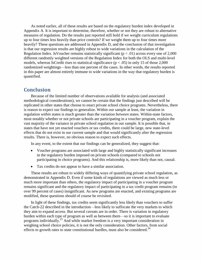
Appendix A. Quantifying Private School Regulation

Table A1 presents the quantification system for our Regulation Index variable. Table 2, in

the body of the text, presents the Regulation Index category values for each group of private

schools, by program participation and state, based on the relevant legislation.

For each of nine categories, values between 0 and 6 are assigned based on the

severity/number of the corresponding regulations. Some categories, such as Price Controls, are

presented as a simple list of descriptions and their scores, while others are presented as a

combination of base scores and score modifiers. These two presentations are functionally

equivalent, and the latter approach is used merely to save space (because, otherwise, we would

have to list all the combinations of the base scores and the modifiers as separate rows in the

table). A discussion of the rationale for including each regulation category in the index follows

the table.

Table A1. Regulation Index Scoring, by Category

Price Controls No price controls 0 Partial controls 3 Fixed price, no co-pay 6 Admissions Controls Unfettered 0 Must use random lottery or first come first served for some grades 3 No autonomy (random lottery or FCFS admissions for all students) 6 Cannot cater to specific religious constituencies +1 Some form of enrollment cap +2 Curriculum Regulations (base score) No curriculum guidelines 0 Limited general framework 2 Extensive or detailed framework 4 Extensive and detailed framework 6 Curriculum Regulations (mod factors--min total = 0) Some exemptions (e.g., rules only apply > enrollment) -1 Instruction must be in English +1 Testing Requirements (base score) No testing requirement 0 Some testing required, but schools choose tests 2 Some specific tests required 4 Specific high-stakes tests required 6 Testing Requirements (mod factor--max total = 6) School must publish results +1

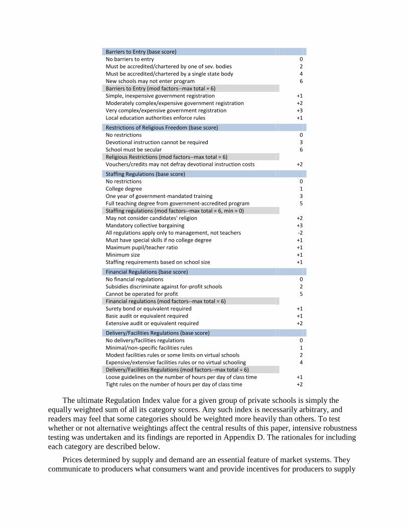
Barriers to Entry (base score) No barriers to entry 0 Must be accredited/chartered by one of sev. bodies 2 Must be accredited/chartered by a single state body 4 New schools may not enter program 6 Barriers to Entry (mod factors--max total = 6) Simple, inexpensive government registration +1 Moderately complex/expensive government registration +2 Very complex/expensive government registration +3 Local education authorities enforce rules +1 Restrictions of Religious Freedom (base score) No restrictions 0 Devotional instruction cannot be required 3 School must be secular 6 Religious Restrictions (mod factors--max total = 6) Vouchers/credits may not defray devotional instruction costs +2 Staffing Regulations (base score) No restrictions 0 College degree 1 One year of government-mandated training 3 Full teaching degree from government-accredited program 5 Staffing regulations (mod factors--max total = 6, min = 0) May not consider candidates' religion +2 Mandatory collective bargaining +3 All regulations apply only to management, not teachers -2 Must have special skills if no college degree +1 Maximum pupil/teacher ratio +1 Minimum size +1 Staffing requirements based on school size +1 Financial Regulations (base score) No financial regulations 0 Subsidies discriminate against for-profit schools 2 Cannot be operated for profit 5 Financial regulations (mod factors--max total = 6) Surety bond or equivalent required +1 Basic audit or equivalent required +1 Extensive audit or equivalent required +2 Delivery/Facilities Regulations (base score) No delivery/facilities regulations 0 Minimal/non-specific facilities rules 1 Modest facilities rules or some limits on virtual schools 2 Expensive/extensive facilities rules or no virtual schooling 4 Delivery/Facilities Regulations (mod factors--max total = 6) Loose guidelines on the number of hours per day of class time +1 Tight rules on the number of hours per day of class time +2

The ultimate Regulation Index value for a given group of private schools is simply the

equally weighted sum of all its category scores. Any such index is necessarily arbitrary, and

readers may feel that some categories should be weighted more heavily than others. To test

whether or not alternative weightings affect the central results of this paper, intensive robustness

testing was undertaken and its findings are reported in Appendix D. The rationales for including

each category are described below.

Prices determined by supply and demand are an essential feature of market systems. They

communicate to producers what consumers want and provide incentives for producers to supply

the most sought-after goods and services. Without the information and incentives provided by

freely determined prices, the market’s operation is grossly impeded.

Specialization and the division of labor are also core features of markets. It is no

coincidence that they are the first topic of extended discussion in Adam Smith’s The Wealth of

Nations. Without them, the development of specialized expertise is hobbled, and along with it

efficiency and innovation. Admissions regulations that force every school to accept students on a

random lottery basis when oversubscribed interfere with the ability of schools to tailor their

services to particular audiences. This is, moreover, a more severe regulatory burden than that

obtaining within conventional public school systems. Contrary to the common statement that

―public schools accept all comers,‖ public school systems frequently place students that they are

unable to serve in private schools that specialize in educating children with their particular needs.

Hundreds of thousands of students are so placed every year.27

Even in the case of students

without special needs, schools in a given district need not accept any student outside their

catchment area. What the public school system guarantees is thus that every child will be served

somewhere, not that every school will (or will be able to) serve every child.

Curriculum regulations are an obvious further imposition on specialization and the division

of labor. They also undermine the power of consumer choice—if all the instructional offerings in

the marketplace are homogenized, parents no longer have meaningful choice (evoking Henry

Ford’s: ―any color you want, so long as it’s black‖). What is less often recognized is that state-

mandated testing also exerts a homogenizing pressure on what is taught. Reporting poor results

on an official test—even one that does not well reflect a school’s mission—would put it at a

competitive disadvantage. So an art-centric school that posts poor science scores is under

pressure to increase the time and intensity of its science classes in order to avoid a black eye on

official tests, which thereby takes away from its core mission. Though language learning occurs

most easily in younger children, a school that opted to focus on foreign languages and history in

the early grades and then turn to mathematics in the later grades would be at a grave

disadvantage on official mathematics tests in the early grades, creating pressure for it to abandon

its pedagogical mission.

The entry of new firms into a marketplace is a lynch-pin of innovation and productivity

growth, both directly and indirectly. New firms that survive their initial start-up phase are usually

better able to use the latest technology and thus to enjoy higher productivity growth than

established firms. And, as Schumpeter argued28

and subsequent research has confirmed,29

the

entry of these new firms—and even the mere threat of their entry—is enough to drive existing

firms to pursue innovation and seek productivity growth internally. Those existing firms that are

unable to keep up the pace of improvement are supplanted by their competitors—a process

Schumpeter termed ―creative destruction.‖ Regulations inhibiting entry of new schools are thus

inimical to innovation and efficiency improvements.

There is unquestionably very substantial demand for religious schooling in the United

States, and religious (particularly Catholic) schools are generally found to be more efficient,

have equal or better academic achievement, and have higher attainment than public schools.

James Coleman30

and later Bryk, Lee and Holland31

ascribe some of these advantages to the

ability of religious schools to create institutional cohesion and a sense of community based

around their faith. Inhibiting religious freedom in education is thus not only deleterious to

parental choice, it is also likely to be injurious to school effectiveness and efficiency.

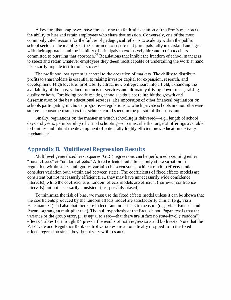
A key tool that employers have for securing the faithful execution of the firm’s mission is

the ability to hire and retain employees who share that mission. Conversely, one of the most

commonly cited reasons for the failure of pedagogical reforms to scale up within the public

school sector is the inability of the reformers to ensure that principals fully understand and agree

with their approach, and the inability of principals to exclusively hire and retain teachers

committed to pursuing that approach.32

Regulations that inhibit the freedom of school managers

to select and retain whatever employees they deem most capable of undertaking the work at hand

necessarily impede institutional success.

The profit and loss system is central to the operation of markets. The ability to distribute

profits to shareholders is essential to raising investor capital for expansion, research, and

development. High levels of profitability attract new entrepreneurs into a field, expanding the

availability of the most valued products or services and ultimately driving down prices, raising

quality or both. Forbidding profit-making schools is thus apt to inhibit the growth and

dissemination of the best educational services. The imposition of other financial regulations on

schools participating in choice programs—regulations to which private schools are not otherwise

subject—consume resources that schools could spend in the pursuit of their mission.

Finally, regulations on the manner in which schooling is delivered—e.g., length of school

days and years, permissibility of virtual schooling—circumscribe the range of offerings available

to families and inhibit the development of potentially highly efficient new education delivery

mechanisms.

Appendix B. Multilevel Regression Results Multilevel generalized least squares (GLS) regressions can be performed assuming either

―fixed effects‖ or ―random effects.‖ A fixed effects model looks only at the variation in

regulation within states and ignores variation between states, while a random effects model

considers variation both within and between states. The coefficients of fixed effects models are

consistent but not necessarily efficient (i.e., they may have unnecessarily wide confidence

intervals), while the coefficients of random effects models are efficient (narrower confidence

intervals) but not necessarily consistent (i.e., possibly biased).

To minimize the risk of bias, we must use the fixed effects model unless it can be shown that

the coefficients produced by the random effects model are satisfactorily similar (e.g., via a

Hausman test) and also that there are indeed random effects to measure (e.g., via a Breusch and

Pagan Lagrangian multiplier test). The null hypothesis of the Breusch and Pagan test is that the

variance of the group error, µi, is equal to zero—that there are in fact no state-level (―random‖)

effects. Tables B1 through B4 present the results of both regressions and both tests. Note that the

PctPrivate and RegulationRank control variables are automatically dropped from the fixed

effects regression since they do not vary within states.

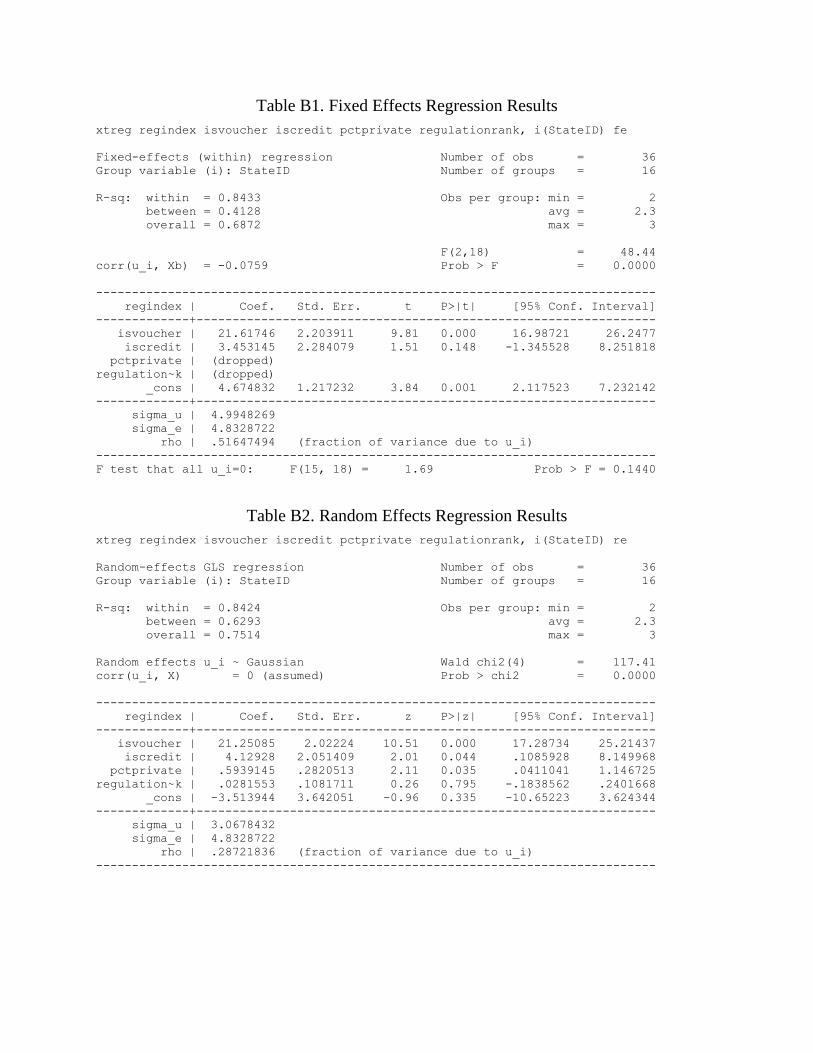
Table B1. Fixed Effects Regression Results

xtreg regindex isvoucher iscredit pctprivate regulationrank, i(StateID) fe

Fixed-effects (within) regression Number of obs = 36

Group variable (i): StateID Number of groups = 16

R-sq: within = 0.8433 Obs per group: min = 2

between = 0.4128 avg = 2.3

overall = 0.6872 max = 3

F(2,18) = 48.44

corr(u_i, Xb) = -0.0759 Prob > F = 0.0000

------------------------------------------------------------------------------

regindex | Coef. Std. Err. t P>|t| [95% Conf. Interval]

-------------+----------------------------------------------------------------

isvoucher | 21.61746 2.203911 9.81 0.000 16.98721 26.2477

iscredit | 3.453145 2.284079 1.51 0.148 -1.345528 8.251818

pctprivate | (dropped)

regulation~k | (dropped)

_cons | 4.674832 1.217232 3.84 0.001 2.117523 7.232142

-------------+----------------------------------------------------------------

sigma_u | 4.9948269

sigma_e | 4.8328722

rho | .51647494 (fraction of variance due to u_i)

------------------------------------------------------------------------------

F test that all u_i=0: F(15, 18) = 1.69 Prob > F = 0.1440

Table B2. Random Effects Regression Results

xtreg regindex isvoucher iscredit pctprivate regulationrank, i(StateID) re

Random-effects GLS regression Number of obs = 36

Group variable (i): StateID Number of groups = 16

R-sq: within = 0.8424 Obs per group: min = 2

between = 0.6293 avg = 2.3

overall = 0.7514 max = 3

Random effects u_i ~ Gaussian Wald chi2(4) = 117.41

corr(u_i, X) = 0 (assumed) Prob > chi2 = 0.0000

------------------------------------------------------------------------------

regindex | Coef. Std. Err. z P>|z| [95% Conf. Interval]

-------------+----------------------------------------------------------------

isvoucher | 21.25085 2.02224 10.51 0.000 17.28734 25.21437

iscredit | 4.12928 2.051409 2.01 0.044 .1085928 8.149968

pctprivate | .5939145 .2820513 2.11 0.035 .0411041 1.146725

regulation~k | .0281553 .1081711 0.26 0.795 -.1838562 .2401668

_cons | -3.513944 3.642051 -0.96 0.335 -10.65223 3.624344

-------------+----------------------------------------------------------------

sigma_u | 3.0678432

sigma_e | 4.8328722

rho | .28721836 (fraction of variance due to u_i)

------------------------------------------------------------------------------

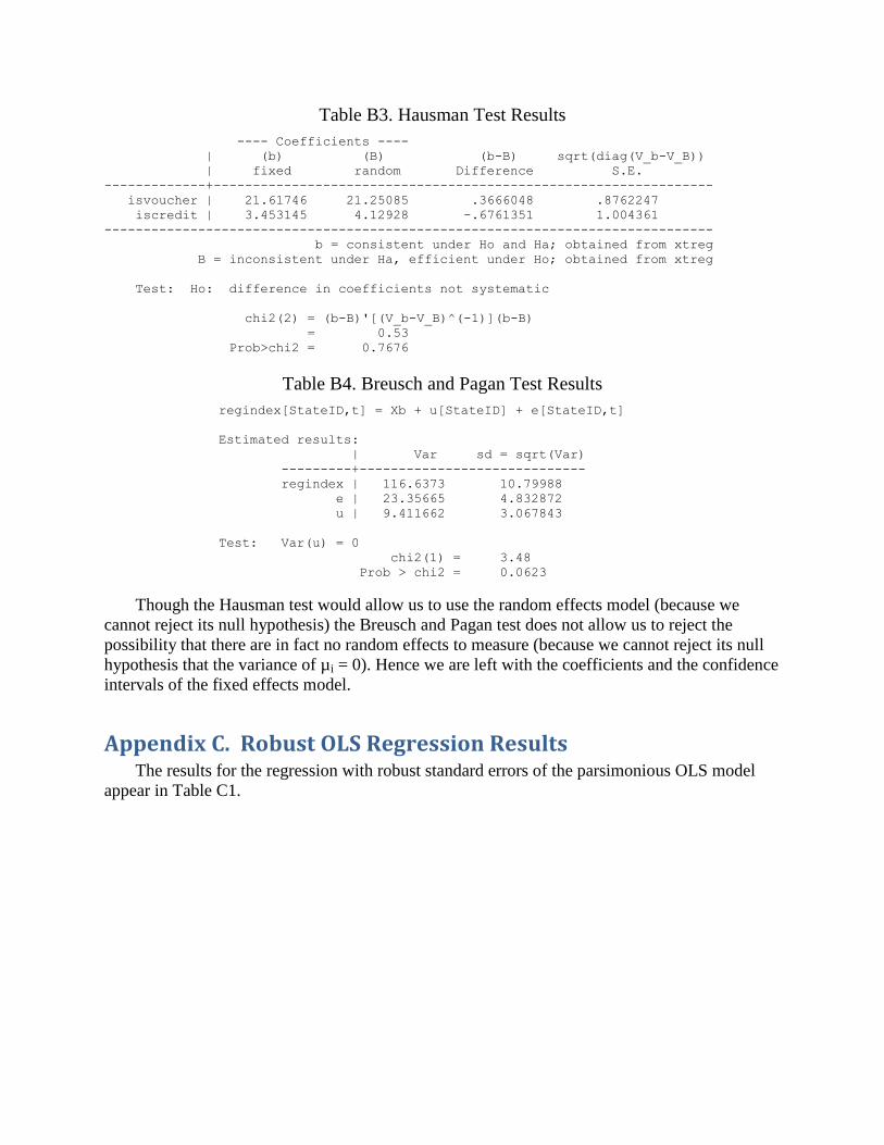
Table B3. Hausman Test Results

---- Coefficients ----

| (b) (B) (b-B) sqrt(diag(V_b-V_B))

| fixed random Difference S.E.

-------------+----------------------------------------------------------------

isvoucher | 21.61746 21.25085 .3666048 .8762247

iscredit | 3.453145 4.12928 -.6761351 1.004361

------------------------------------------------------------------------------

b = consistent under Ho and Ha; obtained from xtreg

B = inconsistent under Ha, efficient under Ho; obtained from xtreg

Test: Ho: difference in coefficients not systematic

chi2(2) = (b-B)'[(V_b-V_B)^(-1)](b-B)

= 0.53

Prob>chi2 = 0.7676

Table B4. Breusch and Pagan Test Results

regindex[StateID,t] = Xb + u[StateID] + e[StateID,t]

Estimated results:

| Var sd = sqrt(Var)

---------+-----------------------------

regindex | 116.6373 10.79988

e | 23.35665 4.832872

u | 9.411662 3.067843

Test: Var(u) = 0

chi2(1) = 3.48

Prob > chi2 = 0.0623

Though the Hausman test would allow us to use the random effects model (because we

cannot reject its null hypothesis) the Breusch and Pagan test does not allow us to reject the

possibility that there are in fact no random effects to measure (because we cannot reject its null

hypothesis that the variance of µi = 0). Hence we are left with the coefficients and the confidence

intervals of the fixed effects model.

Appendix C. Robust OLS Regression Results The results for the regression with robust standard errors of the parsimonious OLS model

appear in Table C1.

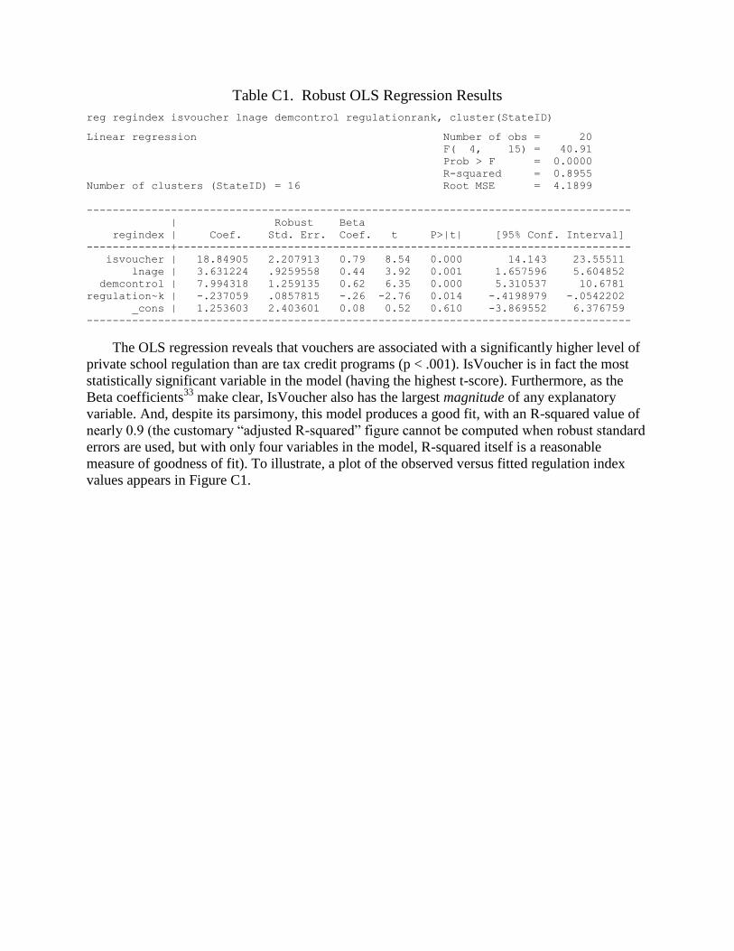
Table C1. Robust OLS Regression Results

reg regindex isvoucher lnage demcontrol regulationrank, cluster(StateID)

Linear regression Number of obs = 20

F( 4, 15) = 40.91

Prob > F = 0.0000

R-squared = 0.8955

Number of clusters (StateID) = 16 Root MSE = 4.1899

------------------------------------------------------------------------------------

| Robust Beta

regindex | Coef. Std. Err. Coef. t P>|t| [95% Conf. Interval]

-------------+----------------------------------------------------------------------

isvoucher | 18.84905 2.207913 0.79 8.54 0.000 14.143 23.55511

lnage | 3.631224 .9259558 0.44 3.92 0.001 1.657596 5.604852

demcontrol | 7.994318 1.259135 0.62 6.35 0.000 5.310537 10.6781

regulation~k | -.237059 .0857815 -.26 -2.76 0.014 -.4198979 -.0542202

_cons | 1.253603 2.403601 0.08 0.52 0.610 -3.869552 6.376759

------------------------------------------------------------------------------------

The OLS regression reveals that vouchers are associated with a significantly higher level of

private school regulation than are tax credit programs (p < .001). IsVoucher is in fact the most

statistically significant variable in the model (having the highest t-score). Furthermore, as the

Beta coefficients33

make clear, IsVoucher also has the largest magnitude of any explanatory

variable. And, despite its parsimony, this model produces a good fit, with an R-squared value of

nearly 0.9 (the customary ―adjusted R-squared‖ figure cannot be computed when robust standard

errors are used, but with only four variables in the model, R-squared itself is a reasonable

measure of goodness of fit). To illustrate, a plot of the observed versus fitted regulation index

values appears in Figure C1.

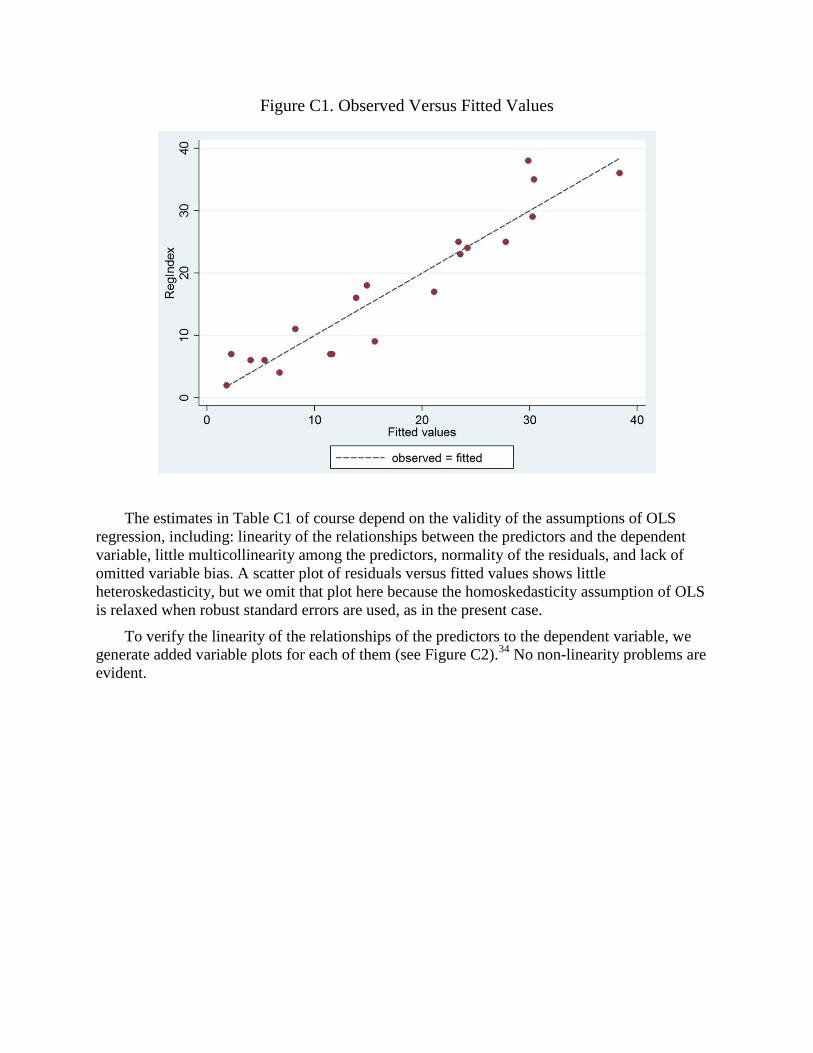
Figure C1. Observed Versus Fitted Values

The estimates in Table C1 of course depend on the validity of the assumptions of OLS

regression, including: linearity of the relationships between the predictors and the dependent

variable, little multicollinearity among the predictors, normality of the residuals, and lack of

omitted variable bias. A scatter plot of residuals versus fitted values shows little

heteroskedasticity, but we omit that plot here because the homoskedasticity assumption of OLS

is relaxed when robust standard errors are used, as in the present case.

To verify the linearity of the relationships of the predictors to the dependent variable, we

generate added variable plots for each of them (see Figure C2).34

No non-linearity problems are

evident.

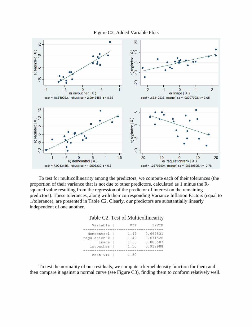
Figure C2. Added Variable Plots

To test for multicollinearity among the predictors, we compute each of their tolerances (the

proportion of their variance that is not due to other predictors, calculated as 1 minus the R‐squared value resulting from the regression of the predictor of interest on the remaining

predictors). These tolerances, along with their corresponding Variance Inflation Factors (equal to

1/tolerance), are presented in Table C2. Clearly, our predictors are substantially linearly

independent of one another.

Table C2. Test of Multicollinearity

Variable | VIF 1/VIF

-------------+----------------------

demcontrol | 1.49 0.669531

regulation~k | 1.49 0.671526

lnage | 1.13 0.886587

isvoucher | 1.10 0.912988

-------------+----------------------

Mean VIF | 1.30

To test the normality of our residuals, we compute a kernel density function for them and

then compare it against a normal curve (see Figure C3), finding them to conform relatively well.

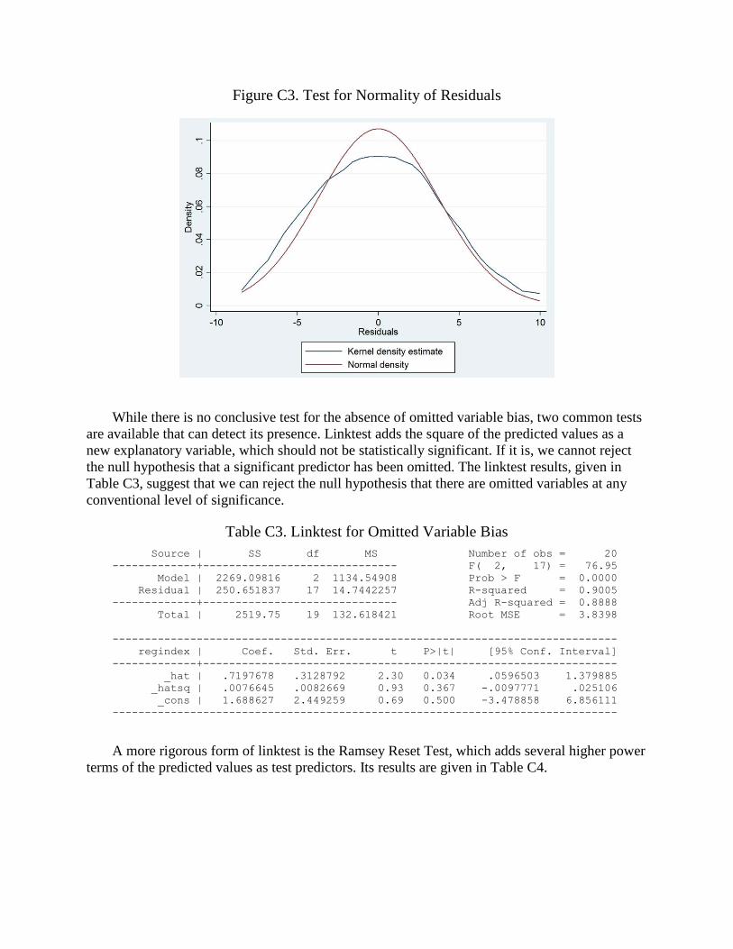
Figure C3. Test for Normality of Residuals

While there is no conclusive test for the absence of omitted variable bias, two common tests

are available that can detect its presence. Linktest adds the square of the predicted values as a

new explanatory variable, which should not be statistically significant. If it is, we cannot reject

the null hypothesis that a significant predictor has been omitted. The linktest results, given in

Table C3, suggest that we can reject the null hypothesis that there are omitted variables at any

conventional level of significance.

Table C3. Linktest for Omitted Variable Bias

Source | SS df MS Number of obs = 20

-------------+------------------------------ F( 2, 17) = 76.95

Model | 2269.09816 2 1134.54908 Prob > F = 0.0000

Residual | 250.651837 17 14.7442257 R-squared = 0.9005

-------------+------------------------------ Adj R-squared = 0.8888

Total | 2519.75 19 132.618421 Root MSE = 3.8398

------------------------------------------------------------------------------

regindex | Coef. Std. Err. t P>|t| [95% Conf. Interval]

-------------+----------------------------------------------------------------

_hat | .7197678 .3128792 2.30 0.034 .0596503 1.379885

_hatsq | .0076645 .0082669 0.93 0.367 -.0097771 .025106

_cons | 1.688627 2.449259 0.69 0.500 -3.478858 6.856111

------------------------------------------------------------------------------

A more rigorous form of linktest is the Ramsey Reset Test, which adds several higher power

terms of the predicted values as test predictors. Its results are given in Table C4.

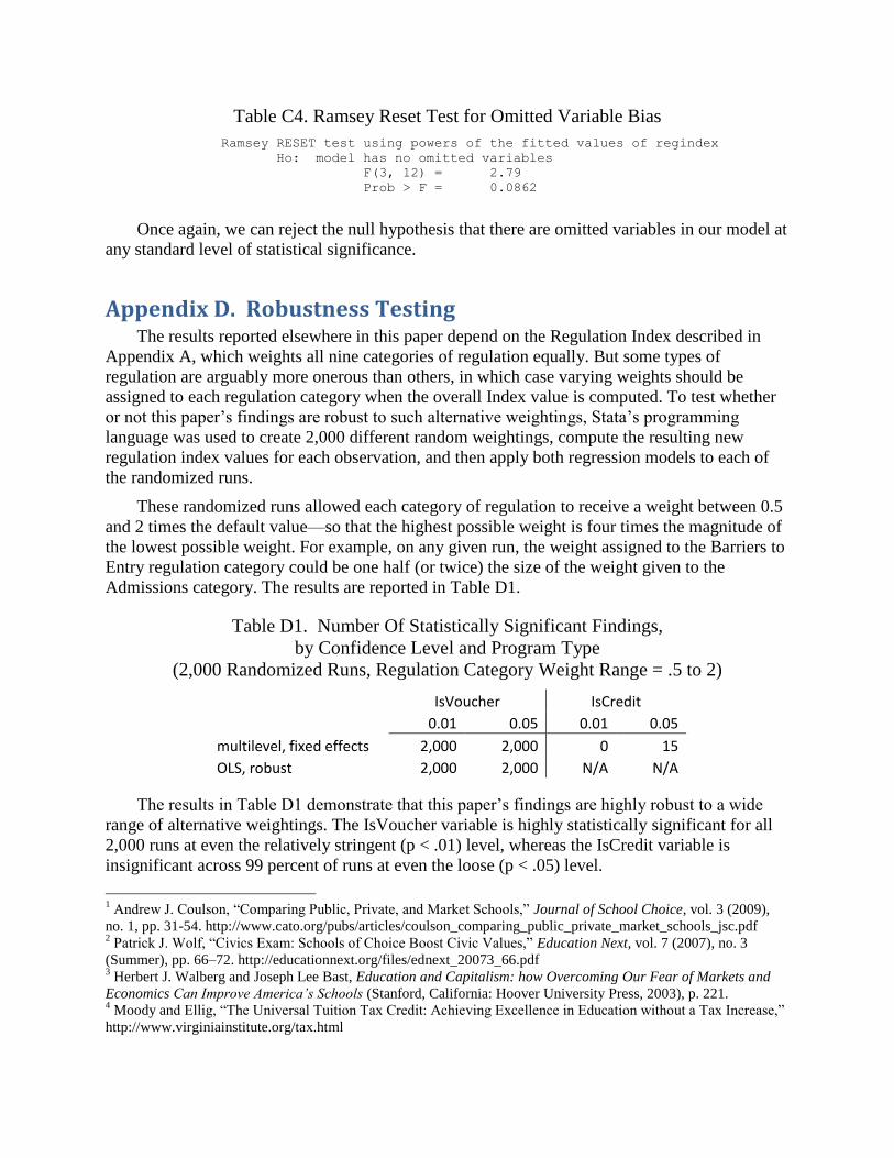
Table C4. Ramsey Reset Test for Omitted Variable Bias

Ramsey RESET test using powers of the fitted values of regindex

Ho: model has no omitted variables

F(3, 12) = 2.79

Prob > F = 0.0862

Once again, we can reject the null hypothesis that there are omitted variables in our model at

any standard level of statistical significance.

Appendix D. Robustness Testing The results reported elsewhere in this paper depend on the Regulation Index described in

Appendix A, which weights all nine categories of regulation equally. But some types of

regulation are arguably more onerous than others, in which case varying weights should be

assigned to each regulation category when the overall Index value is computed. To test whether

or not this paper’s findings are robust to such alternative weightings, Stata’s programming

language was used to create 2,000 different random weightings, compute the resulting new

regulation index values for each observation, and then apply both regression models to each of

the randomized runs.

These randomized runs allowed each category of regulation to receive a weight between 0.5

and 2 times the default value—so that the highest possible weight is four times the magnitude of

the lowest possible weight. For example, on any given run, the weight assigned to the Barriers to

Entry regulation category could be one half (or twice) the size of the weight given to the

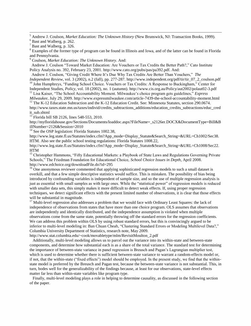
Admissions category. The results are reported in Table D1.

Table D1. Number Of Statistically Significant Findings,

by Confidence Level and Program Type

(2,000 Randomized Runs, Regulation Category Weight Range = .5 to 2)

IsVoucher IsCredit

0.01 0.05 0.01 0.05

multilevel, fixed effects 2,000 2,000 0 15

OLS, robust 2,000 2,000 N/A N/A

The results in Table D1 demonstrate that this paper’s findings are highly robust to a wide

range of alternative weightings. The IsVoucher variable is highly statistically significant for all

2,000 runs at even the relatively stringent (p < .01) level, whereas the IsCredit variable is

insignificant across 99 percent of runs at even the loose (p < .05) level.

1 Andrew J. Coulson, ―Comparing Public, Private, and Market Schools,‖ Journal of School Choice, vol. 3 (2009),

no. 1, pp. 31-54. http://www.cato.org/pubs/articles/coulson_comparing_public_private_market_schools_jsc.pdf 2 Patrick J. Wolf, ―Civics Exam: Schools of Choice Boost Civic Values,‖ Education Next, vol. 7 (2007), no. 3

(Summer), pp. 66–72. http://educationnext.org/files/ednext_20073_66.pdf 3 Herbert J. Walberg and Joseph Lee Bast, Education and Capitalism: how Overcoming Our Fear of Markets and

Economics Can Improve America’s Schools (Stanford, California: Hoover University Press, 2003), p. 221. 4 Moody and Ellig, ―The Universal Tuition Tax Credit: Achieving Excellence in Education without a Tax Increase,‖

http://www.virginiainstitute.org/tax.html

5 Andrew J. Coulson, Market Education: The Unknown History (New Brunswick, NJ: Transaction Books, 1999).

6 Bast and Walberg, p. 262.

7 Bast and Walberg, p. 326.

8 Examples of the former type of program can be found in Illinois and Iowa, and of the latter can be found in Florida

and Pennsylvania. 9 Coulson, Market Education: The Unknown History. And:

Andrew J. Coulson ―Toward Market Education: Are Vouchers or Tax Credits the Better Path?,‖ Cato Institute

Policy Analysis no. 392, February 23, 2001. http://www.cato.org/pubs/pas/pa392.pdf. And:

Andrew J. Coulson, ―Giving Credit Where It’s Due Why Tax Credits Are Better Than Vouchers,‖ The

Independent Review, vol. 3 (2002), n.2 (fall), pp. 277-287. http://www.independent.org/pdf/tir/tir_07_2_coulson.pdf 10

John Humphreys, ―Funding School Choice. Vouchers or Tax Credits: A Response to Buckingham,‖ Center for

Independent Studies, Policy, vol. 18 (2002), no. 1 (autumn). http://www.cis.org.au/Policy/aut2002/polaut02-3.pdf 11

Lisa Kaiser, ―The School Accountability Moment. Milwaukee’s choice program gets guidelines,‖ Express

Milwaukee, July 29, 2009. http://www.expressmilwaukee.com/article-7439-the-school-accountability-moment.html 12

The K-12 Education Subtraction and the K-12 Education Credit. See: Minnesota Statutes, section 290.0674.

http://www.taxes.state.mn.us/taxes/individ/credits_subtractions_additions/education_credits_subtractions/educ_cred

it_sub.shtml 13

Florida bill SB 2126, lines 548-553, 2010.

http://myfloridahouse.gov/Sections/Documents/loaddoc.aspx?FileName=_s2126er.DOCX&DocumentType=Bill&B

illNumber=2126&Session=2010 14

See the OSP legislation: Florida Statutes 1002.38,

http://www.leg.state.fl.us/Statutes/index.cfm?App_mode=Display_Statute&Search_String=&URL=Ch1002/Sec38.

HTM. Also see the public school testing regulations: Florida Statutes 1008.22,

http://www.leg.state.fl.us/Statutes/index.cfm?App_mode=Display_Statute&Search_String=&URL=Ch1008/Sec22.

HTM 15

Christopher Hammons, ―Fifty Educational Markets: a Playbook of State Laws and Regulations Governing Private

Schools,‖ The Friedman Foundation for Educational Choice, School Choice Issues in Depth, April 2008.

http://www.edchoice.org/downloadFile.do?id=295 16

One anonymous reviewer commented that applying sophisticated regression models to such a small dataset is

overkill, and that a few simple descriptive statistics would suffice. This is mistaken. The possibility of bias being

introduced by confounding variables is independent of sample size, and so the use of multiple regression analysis is

just as essential with small samples as with large ones. While the ―statistical power‖ of regression models is reduced

with smaller data sets, this simply makes it more difficult to detect weak effects. If, using proper regression

techniques, we detect significant effects with the present limited number of observations, it is clear that those effects

will be substantial in magnitude. 17

Multi-level regression also addresses a problem that we would face with Ordinary Least Squares: the lack of

independence of observations from states that have more than one choice program. OLS assumes that observations

are independently and identically distributed, and the independence assumption is violated when multiple

observations come from the same state, potentially throwing off the standard errors for the regression coefficients.

We can address this problem within OLS by using robust standard errors, but this is convincingly argued to be

inferior to multi-level modeling in: Ban Chuan Cheah, ―Clustering Standard Errors or Modeling Multilevel Data?,‖

Columbia University Department of Statistics, research note, May 2009.

http://www.stat.columbia.edu/~cook/movabletype/mlm/RevisitMoulton_2.pdf

Additionally, multi-level modeling allows us to parcel out the variance into its within-state and between-state

components, and determine how substantial each is as a share of the total variance. The standard test for determining

the importance of between-state variance in panel regression is Breusch and Pagan’s Lagrangian multiplier test,

which is used to determine whether there is sufficient between-state variance to warrant a random-effects model or,

if not, that the within-state (―fixed effects‖) model should be employed. In the present study, we find that the within-

state model is preferred by the Breusch and Pagan test, because the between-state variance is not substantial. This, in

turn, bodes well for the generalizability of the findings because, at least for our observations, state-level effects

matter far less than within-state variables like program type.

Finally, multi-level modeling plays a role in helping to determine causality, as discussed in the following section

of the paper.

18

The DefaultReg variable cannot be included in a regression in which the data set includes observations of private

schools not participating in choice programs, because doing so would violate the recursivity rule of OLS

regression—the dependent variable would be identical (and causally linked) to the DefaultReg values for all the no-

choice-program observations. 19

Douglas M. Hawkins, ―The Problem of Overfitting,‖ Journal of Chemical Information and Computer Sciences,

Vol. 44( 2004), No. 1, pp. 1–12. 20

The predictor of interest, IsVoucher, plus the nine control variables. 21

For a discussion of Mallow’s Cp, see: J. D. Dobson, Applied Multivariate Data Analysis. Volume I: Regression

and Experimental Design (New York: Springer-Verlag, 1991), p. 268-69. 22

For a brief explanation of these criteria, see: Christopher F. Baum, An Introduction to Modern Econometrics

Using Stata (College Station, Texas: Stata Press, 2006), p. 79. 23

For a discussion of the Stata ―cluster()‖ command, see: ―Stata Library: Analyzing Correlated (Clustered) Data,‖

http://www.ats.ucla.edu/stat/stata/library/cpsu.htm. 24

See, for instance, McFadden (1999, p. 6): ―the 2SLS estimator is also biased if we let the number of instruments

grow linearly with sample size. This shows that for the IV [Instrumental Variable] asymptotic theory to be a good

approximation, n must be much larger than j [where j is the number of predictors in stage 1]. One rule-of-thumb for

IV is that n - j should exceed 40, and should grow linearly with n in order to have the large-sample approximations

to the IV distribution work well.‖ Daniel McFadden, Economics 240B Course Reader, Chapter 4, Department of

Economics, University of California at Berkeley. http://elsa.berkeley.edu/~mcfadden/e240b_f01/ch4.pdf 25

Opposed by the Obama administration and by all but a handful of Democrats in Congress, funding for this

program was sunset in 2010, and the program will cease to operate when its existing students have graduated. 26

See, for instance: Adam B. Schaeffer, ―The Public Education Tax Credit,‖ Cato Policy Analysis no. 605,

December 2007. http://www.cato.org/pub_display.php?pub_id=8812. And,

Andrew J. Coulson, ―Forging Consensus: Can the School Choice Movement Come together on an Explicit Goal

and a Plan for Achieving It?‖ Mackinac Center for Public Policy, Research report, April 30, 2004.

http://www.mackinac.org/6517 27

Janet R. Beales and Thomas F. Bertonneau, ―Do Private Schools Serve Difficult-to-Educate Students?,‖ Mackinac

Center for Public Policy, research report, October 1, 1997. See also: ―Jay P. Greene and Greg Forster, ―Effects of

Funding Incentives on Special Educaiton Enrollment,‖ Manhattan Institute Civic Report no. 32, December 2002. 28

Joseph Schumpeter, Capitalism, Socialism and Democracy, (New York: Harper and Brothers, 1950). 29

See, for example, Eric Bartelsman, John Haltiwanger and Stefano Scarpetta, ―Microeconomic Evidence of

Creative Destruction in Industrial and Developing Countries,‖ World Bank working paper, October 2004.

http://siteresources.worldbank.org/INTWDR2005/Resources/creative_destruction.pdf 30

See, for instance: James S. Coleman, Equality and Achievement in Education (Boulder, Colorado: Westview

Press, 1990). 31

Anthony S. Bryk, Valerie E. Lee, and Peter B. Holland, Catholic Schools and the Common Good (Cambridge,

Massachusetts: Harvard University Press, 1993). 32

Andrew J. Coulson, ―With Clear Eyes, Sincere Hearts and Open Minds: A Second Look at Public Education in

America,‖ research report, Mackinac Center for Public Policy, Michigan, July 27, 2002.

http://www.mackinac.org/4447 33

In order to assess the relative magnitude of the explanatory variable coefficients, all of the variables can be

standardized prior to performing the regression, so that they have a mean of 0 and a standard deviation of 1. The

coefficients thus produced are called beta coefficients, and can be interpreted as follows: a one standard deviation

increase in the standardized explanatory variable is associated with an increase of <beta coefficient> standard

deviations in the dependent variable (which, in this case, is the level of regulation on private schools as measured by

our regulatory index). 34

A good brief explanation of added variable plots can be found in: Alan Heckert, ―Partial Regression Plot,‖ Data

Plot Volume 1, National Institute of Standards and Technology, April 4, 2003.

http://www.itl.nist.gov/div898/software/dataplot/refman1/auxillar/partregr.htm.