Embed Size (px)
Citation preview
ARTICLE IN PRESS
Journal of Monetary Economics 54 (2007) 1163–1212
0304-3932/$ -
doi:10.1016/j
$We than
Dean Croush
Ng, and Tom
and an NBE
comments. A
this paper do�CorrespoE-mail ad
(M. Wei).
URL: htt
gov/research/s
www.elsevier.com/locate/jme
Do macro variables, asset markets, or surveysforecast inflation better?$
Andrew Anga,�, Geert Bekaertb, Min Weic
aColumbia Business School, 805 Uris Hall, 3022 Broadway, New York, NY 10027, USAbColumbia Business School, 802 Uris Hall, 3022 Broadway, New York, NY 10027, USA
cFederal Reserve Board of Governors, Division of Monetary Affairs, Washington, DC 20551, USA
Received 26 July 2005; received in revised form 1 April 2006; accepted 4 April 2006
Available online 10 January 2007
Abstract
Surveys do! We examine the forecasting power of four alternative methods of forecasting U.S.
inflation out-of-sample: time-series ARIMA models; regressions using real activity measures
motivated from the Phillips curve; term structure models that include linear, non-linear, and
arbitrage-free specifications; and survey-based measures. We also investigate several methods of
combining forecasts. Our results show that surveys outperform the other forecasting methods and
that the term structure specifications perform relatively poorly. We find little evidence that
combining forecasts produces superior forecasts to survey information alone. When combining
forecasts, the data consistently places the highest weights on survey information.
r 2006 Elsevier B.V. All rights reserved.
JEL classification: E31; E37; E43; E44
Keywords: ARIMA; Phillips curve; Forecasting; Term structure models; Livingston; SPF
see front matter r 2006 Elsevier B.V. All rights reserved.
.jmoneco.2006.04.006
k Jean Boivin for kindly providing data. We have benefitted from the comments of Todd Clark,
ore, Bob Hodrick, Jonas Fisher, Robin Lumsdaine, Michael McCracken, Antonio Moreno, Serena
Stark, and seminar participants at Columbia University, Goldman Sachs Asset Management, UNC
R meeting. We especially thank the editor, Charles Plosser, and an anonymous referee for excellent
ndrew Ang acknowledges support from the National Science Foundation. The opinions expressed in
not necessarily reflect those of the Federal Reserve Board or the Federal Reserve system.
nding author. Tel.: +1212 854 9154; fax: +1 212 662 8474.
dresses: [email protected] (A. Ang), [email protected] (G. Bekaert), [email protected]
p://www.columbia.edu/�aa610, http://www.gsb.columbia.edu/faculty/gbekaert, http://www.federalreserve.
taff/weiminx.htm.
ARTICLE IN PRESSA. Ang et al. / Journal of Monetary Economics 54 (2007) 1163–12121164
1. Introduction
Obtaining reliable and accurate forecasts of future inflation is crucial for policymakersconducting monetary and fiscal policy; for investors hedging the risk of nominal assets; forfirms making investment decisions and setting prices; and for labor and managementnegotiating wage contracts. Consequently, it is no surprise that a considerable academicliterature evaluates different inflation forecasts and forecasting methods. In particular,economists use four main methods to forecast inflation. The first method is atheoretical,using time series models of the ARIMA variety. The second method builds on theeconomic model of the Phillips curve, leading to forecasting regressions that use realactivity measures. Third, we can forecast inflation using information embedded in assetprices, in particular the term structure of interest rates. Finally, survey-based measures useinformation from agents (consumers or professionals) directly to forecast inflation.In this article, we comprehensively compare and contrast the ability of these four
methods to forecast inflation out of sample. Our approach makes four main contributionsto the literature. First, our analysis is the first to comprehensively compare the fourmethods: time-series forecasts, forecasts based on the Phillips curve, forecasts from theyield curve, and surveys (the Livingston, Michigan, and SPF surveys). The previousliterature has concentrated on only one or two of these different forecastingmethodologies. For example, Stockton and Glassman (1987) show that pure time-seriesmodels out-perform more sophisticated macro models, but do not consider term structuremodels or surveys. Fama and Gibbons (1984) compare term structure forecasts with theLivingston survey, but they do not consider forecasts from macro factors. Whereas Grantand Thomas (1999), Thomas (1999) and Mehra (2002) show that surveys out-performsimple time-series benchmarks for forecasting inflation, none of these studies compares theperformance of survey measures with forecasts from Phillips curve or term structuremodels.The lack of a study comparing these four methods of inflation forecasting implies that
there is no well-accepted set of findings regarding the superiority of a particular forecastingmethod. The most comprehensive study to date, Stock and Watson (1999), finds thatPhillips curve-based forecasts produce the most accurate out-of-sample forecasts of U.S.inflation compared with other macro series and asset prices, using data up to 1996.However, Stock and Watson only briefly compare the Phillips-curve forecasts to theMichigan survey and to simple regressions using term structure information. Stock andWatson do not consider no-arbitrage term structure models, non-linear forecastingmodels, or combined forecasts from all four forecasting methods. Recent work also castsdoubts on the robustness of the Stock–Watson findings. In particular, Atkeson andOhanian (2001), Fisher et al. (2002), Sims (2002), and Cecchetti et al. (2000), among others,show that the accuracy of Phillips curve-based forecasts depends crucially on the sampleperiod. Clark and McCracken (2006) address the issue of how instability in the output gapcoefficients of the Phillips curve affects forecasting power. To assess the stability of theinflation forecasts across different samples, we consider out-of-sample forecasts over boththe post-1985 and post-1995 periods.Our second contribution is to evaluate inflation forecasts implied by arbitrage-free asset
pricing models. Previous studies employing term structure data mostly use only the termspread in simple OLS regressions and usually do not use all available term structure data(see, for example, Mishkin, 1990, 1991; Jorion and Mishkin, 1991; Stock and Watson,
ARTICLE IN PRESSA. Ang et al. / Journal of Monetary Economics 54 (2007) 1163–1212 1165
2003). Frankel and Lown (1994) use a simple weighted average of different term spreads,but they do not impose no-arbitrage restrictions. In contrast to these approaches, wedevelop forecasting models that use all available data and impose no-arbitrage restrictions.Our no-arbitrage term structure models incorporate inflation as a state variable becauseinflation is an integral component of nominal yields. The no-arbitrage framework allowsus to extract forecasts of inflation from data on inflation and asset prices taking intoaccount potential time-varying risk premia.
No-arbitrage constraints are reasonable in a world where hedge funds and investmentbanks routinely eliminate arbitrage opportunities in fixed income securities. Imposingtheoretical no-arbitrage restrictions may also lead to more efficient estimation. Just as Anget al. (2006a) show that no-arbitrage models produce superior forecasts of GDP growth,no-arbitrage restrictions may also produce more accurate forecasts of inflation. Inaddition, this is the first article to investigate non-linear, no-arbitrage models of inflation.We investigate both an empirical regime-switching model incorporating term structureinformation and a no-arbitrage, non-linear term structure model following Ang et al.(2006b) with inflation as a state variable.
Our third contribution is that we thoroughly investigate combined forecasts. Stock andWatson (2002a, 2003), among others, show that the use of aggregate indices of manymacro series measuring real activity produces better forecasts of inflation than individualmacro series. To investigate this further, we also include the (Phillips curve-based) index ofreal activity constructed by Bernanke et al. (2005) from 65 macroeconomic series. Inaddition, several authors (see, e.g., Stock and Watson, 1999; Brave and Fisher, 2004;Wright, 2004) advocate combining several alternative models to forecast inflation. Weinvestigate five different methods of combining forecasts: simple means or medians, OLSbased combinations, and Bayesian estimators with equal or unit weight priors.
Finally, our main focus is forecasting inflation rates. Because of the long-standing debatein macroeconomics on the stationarity of inflation rates, we also explicitly contrast thepredictive power of some non-stationary models to stationary models and consider whetherforecasting inflation changes alters the relative forecasting ability of different models.
Our major empirical results can be summarized as follows. The first major result is thatsurvey forecasts outperform the other three methods in forecasting inflation. That themedian Livingston and SPF survey forecasts do well is perhaps not surprising, becausepresumably many of the best analysts use time-series and Phillips curve models. However,even participants in the Michigan survey who are consumers, not professionals, produceaccurate out-of-sample forecasts, which are only slightly worse than those of theprofessionals in the Livingston and SPF surveys. We also find that the best survey forecastsare the survey median forecasts themselves; adjustments to take into account both linearand non-linear bias yield worse out-of-sample forecasting performance.
Second, term structure information does not generally lead to better forecasts and oftenleads to inferior forecasts than models using only aggregate activity measures. Whereasthis confirms the results in Stock and Watson (1999), our investigation of term structuremodels is much more comprehensive. The relatively poor forecasting performance of termstructure models extends to simple regression specifications, iterated long-horizon VARforecasts, no-arbitrage affine models, and non-linear no-arbitrage models. These resultssuggest that while inflation is very important for explaining the dynamics of the termstructure (see, e.g., Ang et al., 2006b), yield curve information is less important forforecasting future inflation.
ARTICLE IN PRESSA. Ang et al. / Journal of Monetary Economics 54 (2007) 1163–12121166
Our third major finding is that combining forecasts does not generally lead to better out-of-sample forecasting performance than single forecasting models. In particular, simpleaveraging, like using the mean or median of a number of forecasts, does not necessarilyimprove the forecast performance, whereas linear combinations of forecasts with weightscomputed based on past performance and prior information generate the biggest gains.Even the Phillips curve models using the Bernanke et al. (2005) forward-looking aggregatemeasure of real activity mostly do not perform well relative to simpler Phillips curvemodels and never outperform the survey forecasts. The strong success of the surveys inforecasting inflation out-of-sample extends to surveys dominating other models in forecastcombination methods. The data consistently place the highest weights on the surveyforecasts and little weight on other forecasting methods.The remainder of this paper is organized as follows. Section 2 describes the data set. In
Section 3, we describe the time-series models, predictive macro regressions, term structuremodels, and forecasts from survey data, and detail the forecasting methodology. Section 4contains the empirical out-of-sample results. We examine the robustness of our results to anon-stationary inflation specification in Section 5. Finally, Section 6 concludes.
2. Data
2.1. Inflation
We consider four different measures of inflation. The first three are consumer price index(CPI) measures, including CPI-U for all urban consumers, all items (PUNEW), CPI for allurban consumers, all items less shelter (PUXHS) and CPI for all urban consumers, allitems less food and energy (PUXX), which is also called core CPI. The latter two measuresstrip out highly volatile components in order to better reflect underlying price trends (seethe discussion in Quah and Vahey, 1995). The fourth measure is the personal consumptionexpenditure deflator (PCE). While all three surveys forecast a CPI-based inflation measure,PCE inflation features prominently in policy work at the Federal Reserve. All measures areseasonally adjusted and obtained from the Bureau of Labor Statistics website. The sampleperiod is 1952:Q2–2002:Q4 for PUNEW and PUXHS, 1958:Q2–2002:Q4 for PUXX, and1960:Q2–2002:Q4 for PCE.We define the quarterly inflation rate, pt, from t� 1 to t as
pt ¼ lnPt
Pt�1
� �, (1)
where Pt is the inflation index level at the end of the last month of quarter t. We use theterms ‘‘inflation’’ and ‘‘inflation rate’’ interchangeably as defined in Eq. (1). We take onequarter to be our base unit for estimation purposes, but forecast annual inflation, ptþ4;4,from t to tþ 4:
ptþ4;4 ¼ ptþ1 þ ptþ2 þ ptþ3 þ ptþ4, (2)
where pt is the quarterly inflation rate in Eq. (1).Empirical work on inflation has failed to come to a consensus regarding its stationarity
properties. For example, Bryan and Cecchetti (1993) assume a stationary inflation process,while Nelson and Schwert (1977) and Stock and Watson (1999) assume that the inflationprocess has a unit root. Most of our analysis assumes that inflation is stationary for two
ARTICLE IN PRESSA. Ang et al. / Journal of Monetary Economics 54 (2007) 1163–1212 1167
reasons. First, it is difficult to generate non-stationary inflation in standard economicmodels, whether they are monetary in nature, or of the New Keynesian variety (see Fuhrerand Moore, 1995; Holden and Driscoll, 2003). Second, the working paper version of Baiand Ng (2004) recently rejects the null of non-stationarity for inflation. That being said,Cogley and Sargent (2005) and Stock and Watson (2005) find evidence of changes ininflation persistence over time, with a random walk or integrated MA-process providing anaccurate description of inflation dynamics during certain times. Furthermore, the use of aparsimonious non-stationary model may be attractive for forecasting. In particular,Atkeson and Ohanian (2001) have made the random walk a natural benchmark to beat inforecasting exercises. Therefore, we consider whether our results are robust to assumingnon-stationary inflation in Section 5.
Table 1 reports summary statistics for all four measures of inflation for the full sample inPanel A, and the post-1985 sample and the post-1995 sample in Panels B and C,respectively. Our statistics pertain to annual inflation, ptþ4;4, but we sample the dataquarterly. We report the fourth autocorrelation for quarterly inflation, corrðpt;pt�4Þ.Table 1 shows that all four inflation measures are lower and more stable during the lasttwo decades, in common with many other macroeconomic series, including output (seeKim and Nelson, 1999; McConnell and Perez-Quiros, 2000; Stock and Watson, 2002b).Core CPI (PUXX) has the lowest volatility of all the inflation measures. PUXX volatilityranges from 2.56% per annum over the full sample to only 0.24% per annum post-1996.The higher variability of the other measures in the latter part of the sample must be due tofood and energy price changes. In the later sample periods, PCE inflation is, on average,lower than CPI inflation, which may be partly due to its use of a chain weighting incontrast to the other CPI measures which use a fixed basket (see Clark, 1999).
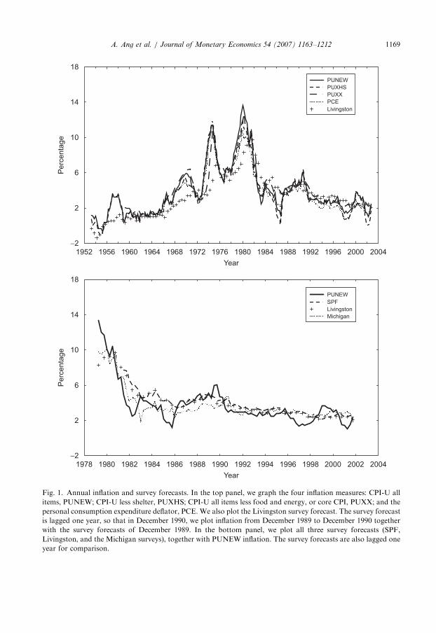
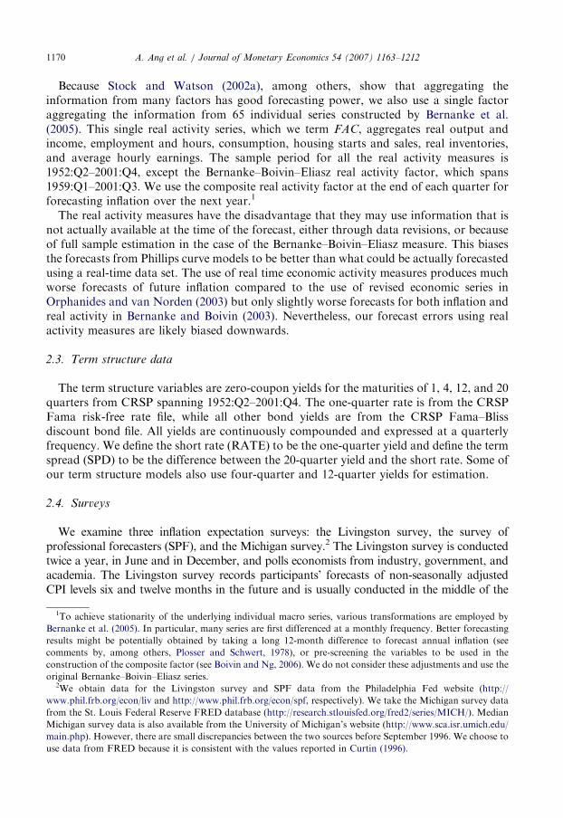
Inflation is somewhat persistent (0.79% for PUNEW over the full sample), but itspersistence decreases over time, as can be seen from the lower autocorrelation coefficientsfor the PUNEW and the PUXHS measures after 1986, and for all measures after 1995. Thecorrelations of the four measures of inflation with each other are all over 75% over the fullsample. The comovement can be clearly seen in the top panel of Fig. 1. Inflation is lowerprior to 1969 and after 1983, but reaches a high of around 14% during the oil crisis of1973–1983. PUXX tracks both PUNEW and PUXHS closely, except during the 1973–1975period, where it is about 2% lower than the other two measures, and after 1985, where itappears to be more stable than the other two measures. During the periods when inflationis decelerating, such as in 1955–1956, 1987–1988, 1998–2000 and most recently 2002–2003,PUNEW declines more gradually than PUXHS, suggesting that housing prices are lessvolatile than the prices of other consumption goods during these periods.
2.2. Real activity measures
We consider six individual series for real activity along with one composite real activityfactor. We compute GDP growth (GDPG) using the seasonally adjusted data on real GDPin billions of chained 2000 dollars. The unemployment rate (UNEMP) is also seasonallyadjusted and computed for the civilian labor force aged 16 years and over. Both real GDPand the unemployment rate are from the Federal Reserve economic data (FRED)database. We compute the output gap either as the detrended log real GDP by removing aquadratic trend as in Gali and Gertler (1999), which we term GAP1, or by using theHodrick–Prescott (1997) filter (with the standard smoothness parameter of 1,600), which
ARTICLE IN PRESS
Table 1
Summary statistics
PUNEW PUXHS PUXX PCE
Panel A: 1952:Q2– 2002:Q4a
Mean 3.84 3.60 4.24 3.84
(0.20) (0.20) (0.19) (0.19)
Standard deviation 2.86 2.78 2.56 2.45
(0.14) (0.14) (0.14) (0.13)
Autocorrelation 0.78 0.74 0.77 0.79
(0.08) (0.09) (0.11) (0.09)
Correlations
PUXHS 0.99
PUXX 0.94 0.91
PCE 0.98 0.98 0.93
Panel B: 1986:Q1– 2002:Q4
Mean 3.09 2.87 3.21 2.58
(0.14) (0.17) (0.12) (0.14)
Standard deviation 1.12 1.37 0.97 1.08
(0.10) (0.12) (0.09) (0.10)
Autocorrelation 0.47 0.37 0.77 0.69
(0.07) (0.10) (0.08) (0.07)
Correlations
PUXHS 0.99
PUXX 0.85 0.79
PCE 0.95 0.93 0.90
Panel C: 1996:Q1– 2002:Q4
Mean 2.27 1.84 2.32 1.70
(0.17) (0.25) (0.05) (0.13)
Standard deviation 0.81 1.19 0.24 0.62
(0.12) (0.17) (0.03) (0.09)
Autocorrelation �0.13 �0.19 �0.38 0.05
(0.23) (0.23) (0.14) (0.18)
Correlations
PUXHS 0.99
PUXX 0.33 0.21
PCE 0.89 0.88 0.19
This table reports various moments of different measures of annual inflation sampled at a quarterly frequency for
different sample periods. PUNEW is CPI-U all items; PUXHS is CPI-U less shelter; PUXX is CPI-U all items less
food and energy, also called core CPI; and PCE is the personal consumption expenditure deflator. All measures
are in annual percentage terms. The autocorrelation reported is the fourth order autocorrelation with the
quarterly inflation data, corrðpt; pt�4Þ. Standard errors reported in parentheses are computed by GMM.aFor PUXX, the start date is 1958:Q2 and for PCE, the start date is 1960:Q2.
A. Ang et al. / Journal of Monetary Economics 54 (2007) 1163–12121168
we term GAP2. At time t, both measures are constructed using only current and past GDPvalues, so the filters are run recursively. We also use the labor income share (LSHR),defined as the ratio of nominal compensation to total nominal output in the U.S. nonfarmbusiness sector. We use two forward-looking indicators: the Stock–Watson (1989)experimental leading index (LI) and their alternative nonfinancial experimental leadingindex-2 (XLI-2).
ARTICLE IN PRESS
18
14
10
6
2
−21952 1956 1960 1964 1968 1972 1976 1980 1984 1988 1992 1996 2000 2004
Year
Perc
enta
ge
Perc
enta
ge
18
14
10
6
2
−21978 1980 1982 1984 1986 1988 1990 1992 1994 1996 1998 2000 2002 2004
Year
PUNEW
PUXHS
PUXX
PCE
Livingston
PUNEW
Livingston
SPF
Michigan
Fig. 1. Annual inflation and survey forecasts. In the top panel, we graph the four inflation measures: CPI-U all
items, PUNEW; CPI-U less shelter, PUXHS; CPI-U all items less food and energy, or core CPI, PUXX; and the
personal consumption expenditure deflator, PCE. We also plot the Livingston survey forecast. The survey forecast
is lagged one year, so that in December 1990, we plot inflation from December 1989 to December 1990 together
with the survey forecasts of December 1989. In the bottom panel, we plot all three survey forecasts (SPF,
Livingston, and the Michigan surveys), together with PUNEW inflation. The survey forecasts are also lagged one
year for comparison.
A. Ang et al. / Journal of Monetary Economics 54 (2007) 1163–1212 1169
ARTICLE IN PRESSA. Ang et al. / Journal of Monetary Economics 54 (2007) 1163–12121170
Because Stock and Watson (2002a), among others, show that aggregating theinformation from many factors has good forecasting power, we also use a single factoraggregating the information from 65 individual series constructed by Bernanke et al.(2005). This single real activity series, which we term FAC, aggregates real output andincome, employment and hours, consumption, housing starts and sales, real inventories,and average hourly earnings. The sample period for all the real activity measures is1952:Q2–2001:Q4, except the Bernanke–Boivin–Eliasz real activity factor, which spans1959:Q1–2001:Q3. We use the composite real activity factor at the end of each quarter forforecasting inflation over the next year.1
The real activity measures have the disadvantage that they may use information that isnot actually available at the time of the forecast, either through data revisions, or becauseof full sample estimation in the case of the Bernanke–Boivin–Eliasz measure. This biasesthe forecasts from Phillips curve models to be better than what could be actually forecastedusing a real-time data set. The use of real time economic activity measures produces muchworse forecasts of future inflation compared to the use of revised economic series inOrphanides and van Norden (2003) but only slightly worse forecasts for both inflation andreal activity in Bernanke and Boivin (2003). Nevertheless, our forecast errors using realactivity measures are likely biased downwards.
2.3. Term structure data
The term structure variables are zero-coupon yields for the maturities of 1, 4, 12, and 20quarters from CRSP spanning 1952:Q2–2001:Q4. The one-quarter rate is from the CRSPFama risk-free rate file, while all other bond yields are from the CRSP Fama–Blissdiscount bond file. All yields are continuously compounded and expressed at a quarterlyfrequency. We define the short rate (RATE) to be the one-quarter yield and define the termspread (SPD) to be the difference between the 20-quarter yield and the short rate. Some ofour term structure models also use four-quarter and 12-quarter yields for estimation.
2.4. Surveys
We examine three inflation expectation surveys: the Livingston survey, the survey ofprofessional forecasters (SPF), and the Michigan survey.2 The Livingston survey is conductedtwice a year, in June and in December, and polls economists from industry, government, andacademia. The Livingston survey records participants’ forecasts of non-seasonally adjustedCPI levels six and twelve months in the future and is usually conducted in the middle of the
1To achieve stationarity of the underlying individual macro series, various transformations are employed by
Bernanke et al. (2005). In particular, many series are first differenced at a monthly frequency. Better forecasting
results might be potentially obtained by taking a long 12-month difference to forecast annual inflation (see
comments by, among others, Plosser and Schwert, 1978), or pre-screening the variables to be used in the
construction of the composite factor (see Boivin and Ng, 2006). We do not consider these adjustments and use the
original Bernanke–Boivin–Eliasz series.2We obtain data for the Livingston survey and SPF data from the Philadelphia Fed website (http://
www.phil.frb.org/econ/liv and http://www.phil.frb.org/econ/spf, respectively). We take the Michigan survey data
from the St. Louis Federal Reserve FRED database (http://research.stlouisfed.org/fred2/series/MICH/). Median
Michigan survey data is also available from the University of Michigan’s website (http://www.sca.isr.umich.edu/
main.php). However, there are small discrepancies between the two sources before September 1996. We choose to
use data from FRED because it is consistent with the values reported in Curtin (1996).
ARTICLE IN PRESSA. Ang et al. / Journal of Monetary Economics 54 (2007) 1163–1212 1171
month. Unlike the Livingston survey, participants in the SPF and the Michigan surveyforecast inflation rates. Participants in the SPF are drawn primarily from business, andforecast changes in the quarterly average of seasonally adjusted CPI-U levels. The SPF isconducted in the middle of every quarter and the sample period for the SPF median forecastsis from 1981:Q3 to 2002:Q4. In contrast to the Livingston survey and SPF, the Michigansurvey is conducted monthly and asks households, rather than professionals, to estimateexpected price changes over the next twelve months. We use the median Michigan surveyforecast of inflation over the next year at the end of each quarter from 1978:Q1 to 2002:Q4.
There are some reporting lags between the time the surveys are taken and the publicdissemination of their results. For the Livingston and the SPF surveys, there is a lag ofabout one week between the due date of the survey and their publication. However, thesereporting lags are largely inconsequential for our purposes. What matters is theinformation set used by the forecasters in predicting future inflation. Clearly, surveyforecasts must use less up to date information than either macro-economic or termstructure forecasts. For example, the Livingston survey forecasters presumably useinformation up to at most the beginning of June and December, and mostly do not evenhave the May and November official CPI numbers available when making a forecast. TheSPF forecasts can only use information up to at most the middle of the quarter and whilewe take the final month of the quarter for the Michigan survey, consumers do not have up-to-date economic data available at the end of the quarter. But, for the economistforecasting annual inflation with the surveys, all survey data is publicly available at the endof each quarter for the SPF and Michigan surveys, and at the end of each semi-annualperiod for the Livingston survey. Together with the slight data advantages present inrevised, fitted macro data, we are in fact biasing the results against survey forecasts.
The Livingston survey is the only survey available for our full sample. In the top panel ofFig. 1, which graphs the full sample of inflation data, we also include the unadjustedmedian Livingston forecasts. We plot the survey forecast lagged one year, so that inDecember 1990, we plot inflation from December 1989 to December 1990 together with thesurvey forecasts of December 1989. The Livingston forecasts broadly track the movementsof inflation, but there are several large movements that the Livingston survey fails to track,for example the pickup in inflation in 1956–1959, 1967–1971, 1972–1975, and 1978–1981.In the bottom panel of Fig. 1, we graph all three survey forecasts of future one-yearinflation together with the annual PUNEW inflation, where the survey forecasts are laggedone year for direct comparison. After 1981, all survey forecasts move reasonably closelytogether and track inflation movements relatively well. Nevertheless, there are still somenotable failures, like the slowdowns in inflation in the early 1980s and in 1996.
3. Forecasting models and methodology
In this section, we describe the forecasting models and describe our statistical tests. In allour out-of-sample forecasting exercises, we forecast future annual inflation. Hence, for allour models, we compute annual inflation forecasts as
Etðptþ4;4Þ ¼ Et
X4i¼1
ptþi
!, (3)
where ptþ4;4 is annual inflation from t to tþ 4 defined in Eq. (2).
ARTICLE IN PRESSA. Ang et al. / Journal of Monetary Economics 54 (2007) 1163–12121172
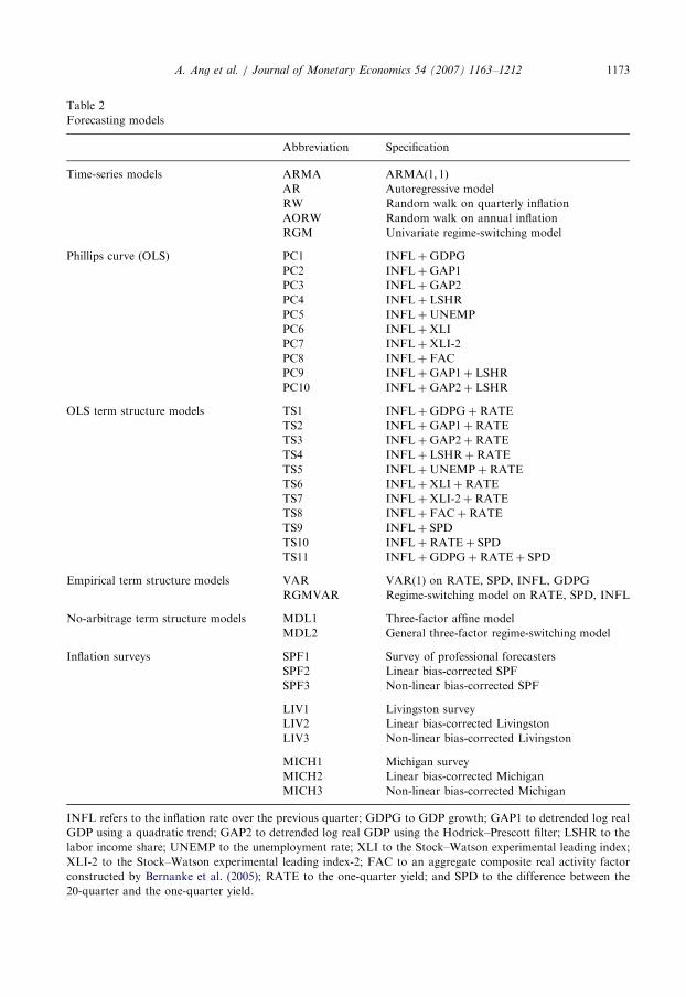
In Sections 3.1–3.4, we describe our 39 forecasting models. Table 2 contains a fullnomenclature. Section 3.1 focuses on time-series models of inflation, which serve as ourbenchmark forecasts; Section 3.2 summarizes our OLS regression models using realactivity macro variables; Section 3.3 describes the term structure models incorporatinginflation data; and finally, Section 3.4 describes our survey forecasts. In Section 3.5, wedefine the out-of-sample periods and list the criteria that we use to assess the performanceof out-of-sample forecasts. Finally, Section 3.6 describes our methodology to combinemodel forecasts.For all models except OLS regressions, we compute implied long-horizon forecasts from
single-period (quarterly) models. While Schorfheide (2005) shows that in theory, iteratedforecasts need not be superior to direct forecasts from horizon-specific models, Marcellinoet al. (2006) document the empirical superiority of iterated forecasts in predicting U.S.macroeconomic series. For the OLS models, we compute the forecasts directly from thelong-horizon regression estimates.
3.1. Time-series models
3.1.1. ARIMA models
If inflation is stationary, the Wold theorem suggests that a parsimonious ARMAðp; qÞmodel may perform well in forecasting. We consider two ARMAðp; qÞ models: anARMAð1; 1Þ model and a pure autoregressive model with p lags, ARðpÞ. The optimal laglength for the AR model is recursively selected using the Schwartz criterion (BIC) on thein-sample data. The motivation for the ARMAð1; 1Þ model derives from a long tradition inrational expectations macroeconomics (see Hamilton, 1985) and finance (see Fama, 1975)that models inflation as the sum of expected inflation and noise. If expected inflationfollows an AR(1) process, then the reduced-form model for inflation is given by anARMAð1; 1Þ model. The ARMAð1; 1Þ model also nicely fits the slowly decayingautocorrelogram of inflation.The specifications of the ARMAð1; 1Þ model,
ptþ1 ¼ mþ fpt þ c�t þ �tþ1, (4)
and the ARðpÞ model,
ptþ1 ¼ mþ f1pt þ f2pt�1 þ � � � þ fppt�pþ1 þ �tþ1, (5)
are entirely standard. The ARMAð1; 1Þ model is estimated by maximum likelihood,conditional on a zero initial residual. We compute the implied inflation level forecast overthe next year expressed at a quarterly frequency. For the ARMAð1; 1Þ model, the forecastis
Etðptþ4;4Þ ¼1
1� f4�
fð1� f4Þ
ð1� fÞ
� �mþ
fð1� f4Þ
ð1� fÞpt þð1� f4
Þcð1� fÞ
�t.
To facilitate the forecasts of annual inflation, we write the ARðpÞ model in first-ordercompanion form
X tþ1 ¼ Aþ FX t þUtþ1,
ARTICLE IN PRESS
Table 2
Forecasting models
Abbreviation Specification
Time-series models ARMA ARMAð1; 1ÞAR Autoregressive model
RW Random walk on quarterly inflation
AORW Random walk on annual inflation
RGM Univariate regime-switching model
Phillips curve (OLS) PC1 INFLþGDPG
PC2 INFLþGAP1
PC3 INFLþGAP2
PC4 INFLþ LSHR
PC5 INFLþUNEMP
PC6 INFLþXLI
PC7 INFLþXLI-2
PC8 INFLþ FAC
PC9 INFLþGAP1þ LSHR
PC10 INFLþGAP2þ LSHR
OLS term structure models TS1 INFLþGDPGþRATE
TS2 INFLþGAP1þRATE
TS3 INFLþGAP2þRATE
TS4 INFLþ LSHRþRATE
TS5 INFLþUNEMPþRATE
TS6 INFLþXLIþRATE
TS7 INFLþXLI-2þRATE
TS8 INFLþ FACþRATE
TS9 INFLþ SPD
TS10 INFLþRATEþ SPD
TS11 INFLþGDPGþRATEþ SPD
Empirical term structure models VAR VAR(1) on RATE, SPD, INFL, GDPG
RGMVAR Regime-switching model on RATE, SPD, INFL
No-arbitrage term structure models MDL1 Three-factor affine model
MDL2 General three-factor regime-switching model
Inflation surveys SPF1 Survey of professional forecasters
SPF2 Linear bias-corrected SPF
SPF3 Non-linear bias-corrected SPF
LIV1 Livingston survey
LIV2 Linear bias-corrected Livingston
LIV3 Non-linear bias-corrected Livingston
MICH1 Michigan survey
MICH2 Linear bias-corrected Michigan
MICH3 Non-linear bias-corrected Michigan
INFL refers to the inflation rate over the previous quarter; GDPG to GDP growth; GAP1 to detrended log real
GDP using a quadratic trend; GAP2 to detrended log real GDP using the Hodrick–Prescott filter; LSHR to the
labor income share; UNEMP to the unemployment rate; XLI to the Stock–Watson experimental leading index;
XLI-2 to the Stock–Watson experimental leading index-2; FAC to an aggregate composite real activity factor
constructed by Bernanke et al. (2005); RATE to the one-quarter yield; and SPD to the difference between the
20-quarter and the one-quarter yield.
A. Ang et al. / Journal of Monetary Economics 54 (2007) 1163–1212 1173
ARTICLE IN PRESSA. Ang et al. / Journal of Monetary Economics 54 (2007) 1163–12121174
where
X t ¼
pt
pt�1
..
.
pt�pþ1
2666664
3777775; A ¼
m
0
..
.
0
266664377775; F ¼
f1 f2 . . . fp
1 0 . . . 0
..
. ... . .
. ...
0 0 . . . 0
266664377775 and Ut ¼
�t
0
..
.
0
266664377775.
Then, the forecast for the ARðpÞ model is given by
Etðptþ4;4Þ ¼ e01ðI � FÞ�1ð4I � FðI � FÞ�1ðI � F4ÞÞAþ e01FðI � FÞ�1ðI � F4ÞX t,
where e1 is a p� 1 selection vector containing a one in the first row and zeros elsewhere.Our third ARIMA benchmark is a random walk (RW) forecast where ptþ1 ¼ pt þ �tþ1,
and Etðptþ4;4Þ ¼ 4pt. Inspired by Atkeson and Ohanian (2001), we also forecast inflationusing a random walk model on annual inflation, where the forecast is given byEtðptþ4;4Þ ¼ pt;4. We denote this forecast as AORW.
3.1.2. Regime-switching models
Evans and Wachtel (1993), Evans and Lewis (1995), and Ang et al. (2006a), amongothers, document regime-switching behavior in inflation. A regime-switching model maypotentially account for non-linearities and structural changes, such as a sudden shift ininflation expectations after a supply shock, or a change in inflation persistence.We estimate the following univariate regime-switching model for inflation, which we
term RGM:
ptþ1 ¼ mðstþ1Þ þ fðstþ1Þpt þ sðstþ1Þ�tþ1. (6)
The regime variable st ¼ 1; 2 follows a Markov chain with constant transition probabilitiesP ¼ Prðstþ1 ¼ 1jst ¼ 1Þ and Q ¼ Prðstþ1 ¼ 2jst ¼ 2Þ. The model can be estimated using theBayesian filter algorithms of Hamilton (1989) and Gray (1996). We compute the impliedannual horizon forecasts of inflation from Eq. (6), assuming that the current regime is theregime that maximizes the probability PrðstjI tÞ. This is a byproduct of the estimationalgorithm.
3.2. Regression forecasts based on the Phillips curve
In standard Phillips curve models of inflation, expected inflation is linked to somemeasure of the output gap. There are both forward- and backward-looking Phillips curvemodels, but ultimately even forward-looking models link expected inflation to the currentinformation set. According to the Phillips curve, measures of real activity should be animportant part of this information set. We avoid the debate regarding the actual measureof the output gap (see, for instance, Gali and Gertler, 1999) by taking an empiricalapproach and using a large number of real activity measures. We choose not to estimatestructural models because the BIC criterion is likely to choose the empirical model bestsuitable for forecasting. Previous work often finds that models with the clearest theoreticaljustification often have poor predictive content (see the literature summary by Stock andWatson, 2003).
ARTICLE IN PRESSA. Ang et al. / Journal of Monetary Economics 54 (2007) 1163–1212 1175
The empirical specification we estimate is
ptþ4;4 ¼ aþ bðLÞ0X t þ �tþ4;4, (7)
where X t combines pt and one or two real activity measures. The lag length in the lagpolynomial bðLÞ is selected by BIC on the in-sample data and is set to be equal across allthe regressors in X t. The chosen specification tends to have two or three lags in ourforecasting exercises. We list the complete set of real activity regressors in Table 2 as PC1to PC10.
In our next section, we extend the information set to include term structure information.Regression models where term structure information is included in X t along with inflationand real activity are potentially consistent with a forward-looking Phillips curve thatincludes inflation and real activity measures in the information set. Such models canapproximate the reduced form of a more sophisticated, forward-looking rationalexpectations Phillips curve model of inflation (see, for instance, Bekaert et al., 2005).
3.3. Models using term structure data
We consider a variety of term structure forecasts, including augmenting the simplePhillips Curve OLS regressions with short rate and term spread variables; long-horizonVAR forecasts; a regime-switching specification; affine term structure models; and termstructure models incorporating regime switches. We outline each of these specificationsin turn.
3.3.1. Linear non-structural models
We begin by augmenting the OLS Phillips Curve models in Eq. (7) with the short rate,RATE, and the term spread, SPD, as regressors in X t. Specifications TS1–TS8 add RATEto the Phillips Curve specifications PC1–PC8. TS9 and TS10 only use inflation and termstructure variables as predictors. TS9 uses inflation and the lagged term spread, producinga forecasting model similar to the specification in Mishkin (1990, 1991). TS10 adds theshort rate to this specification. Finally, TS11 adds GDP growth to the TS10 specification.
We also consider forecasts with a VAR(1) in X t, where X t contains RATE, SPD,GDPG, and pt
X tþ1 ¼ mþ FX t þ �tþ1. (8)
Although the VAR is specified at a quarterly frequency, we compute the annual horizonforecast of inflation implied by the VAR. We denote this forecasting specification as VAR.As Ang et al. (2006a) and Cochrane and Piazzesi (2005) note, a VAR specification can beeconomically motivated from the fact that a reduced-form VAR is equivalent to aGaussian term structure model where the term structure factors are observable yields andcertain assumptions on risk premia apply. Under these restrictions, a VAR coincides witha no-arbitrage term structure model only for those yields included in the VAR. However,the VAR does not impose over-identifying restrictions generated by the term structuremodel for yields not included as factors in the VAR.
3.3.2. An empirical non-linear regime-switching model
A large empirical literature has documented the presence of regime switches in interestrates (see, among others, Hamilton, 1988; Gray, 1996; Bekaert et al., 2001). In particular,
ARTICLE IN PRESSA. Ang et al. / Journal of Monetary Economics 54 (2007) 1163–12121176
Ang et al. (2006a) show that regime-switching models forecast interest rates better thanlinear models. As interest rates reflect information in expected inflation, capturing theregime-switching behavior in interest rates may help in forecasting potentially regime-switching dynamics of inflation.We estimate a regime-switching VAR, denoted as RGMVAR:
X tþ1 ¼ mðstþ1Þ þ FX t þ Sðstþ1Þ�tþ1, (9)
where X t contains RATE, SPD and pt. Similar to the univariate regime-switching model inEq. (6), st ¼ 1 or 2 and follows a Markov chain with constant transition probabilities. Wecompute out-of-sample forecasts from Eq. (9) assuming that the current regime is theregime with the highest probability PrðstjI tÞ.
3.3.3. No-arbitrage term structure models
We estimate two no-arbitrage term structure models. Because such models haveimplications for the complete yield curve, it is straightforward to incorporate additionalinformation from the yield curve into the estimation. Such additional information is absentin the empirical VAR specified in Eq. (8). Concretely, both no-arbitrage models have twolatent variables and quarterly inflation as state variables, denoted by X t. We estimate themodels by maximum likelihood, and following Chen and Scott (1993), assume that the oneand 20-quarter yields are measured without error, and the other four- and 12-quarteryields are measured with error. The estimated models build on Ang et al. (2006b), whoformulate a real pricing kernel asbMtþ1 ¼ expð�rt �
12l0tlt � lt�tþ1Þ. (10)
Here, lt is a 3� 1 real price of risk vector. The real short rate is an affine function of thestate variables. The nominal pricing kernel is defined in the standard way asMtþ1 ¼ bMtþ1 expð�ptþ1Þ. Bonds are priced using the recursion
expð�nynt Þ ¼ Et½Mtþ1 expð�ðn� 1Þyn�1
tþ1 Þ�,
where ynt is the n-quarter zero-coupon bond yield.
The first no-arbitrage model (MDL1) is an affine model in the class of Duffie and Kan(1996) with affine, time-varying risk premia (see Dai and Singleton, 2002; Duffee, 2002)modelled as
lt ¼ l0 þ l1X t, (11)
where l0 is a 3� 1 vector and l1 a 3� 3 diagonal matrix. The state variables follow alinear VAR:
X tþ1 ¼ mþ FX t þ S�tþ1, (12)
The second model (MDL2) incorporates regime switches and is developed by Ang et al.(2006b). Ang, Bekaert and Wei show that this model fits the moments of yields andinflation very well and almost exactly matches the autocorrelogram of inflation. MDL2replaces Eq. (12) with the regime-switching VAR
X tþ1 ¼ mðstþ1Þ þ FX t þ Sðstþ1Þ�tþ1, (13)
and also incorporates regime switches in the prices of risk, replacing lt in Eq. (11) with
ltðstþ1Þ ¼ l0ðstþ1Þ þ l1X t. (14)
ARTICLE IN PRESSA. Ang et al. / Journal of Monetary Economics 54 (2007) 1163–1212 1177
There are four regime variables st ¼ 1; . . . ; 4 in the Ang et al. (2006b) model representingall possible combinations of two regimes of inflation and two regimes of a real latentfactor.
In estimating MDL1 and MDL2, we impose the same parameter restrictions necessaryfor identification as Ang et al. (2006b) do. For both MDL1 and MDL2, we compute out-of-sample forecasts of annual inflation, but the models are estimated using quarterly data.
3.4. Survey forecasts
We produce estimates of Etðptþ4;4Þ from the Livingston, SPF, and the Michigan surveys.We denote the actual forecasts from the SPF, Livingston and Michigan surveys as SPF1,LIV1, and MCH1, respectively.
3.4.1. Producing forecasts from survey data
Participants in the Livingston survey are asked to forecast a CPI level (not an inflationrate). Given the timing of the survey, Carlson (1977) carefully studies the forecasts ofindividual participants in the Livingston survey and finds that the participants generallyforecast inflation over the next 14 months. We follow Thomas (1999) and Mehra (2002)and adjust the raw Livingston forecasts by a factor of 12=14 to obtain an annual inflationforecast.
Participants in both the SPF and the Michigan surveys do not forecast log year-on-yearCPI levels according to the definition of inflation in Eq. (1). Instead, the surveys recordsimple expected inflation changes, EtðPtþ4=Pt � 1Þ. This differs from EtðlogPtþ4=PtÞ by aJensen’s inequality term. In addition, the SPF participants are asked to forecast changes inthe quarterly average of seasonally adjusted PUNEW (CPI-U), as opposed to end-of-quarter changes in CPI levels. In both the SPF and the Michigan survey, we cannotdirectly recover forecasts of expected log changes in CPI levels. Instead, we directly use theSPF and Michigan survey forecasts to represent forecasts of future annual inflation asdefined in Eq. (3). We expect that the effects of these measurement problems are small.3 Inany case, the Jensen’s term biases our survey forecasts upwards, imparting a conservativeupward bias to our root mean squared error (RMSE) statistics.
3.4.2. Adjusting surveys for bias
Several authors, including Thomas (1999), Mehra (2002), and Souleles (2004), documentthat survey forecasts are biased. We take into account the survey bias by estimating a1 andb1 in the regressions:
ptþ4;4 ¼ a1 þ b1fSt þ �tþ4;4, (15)
where f St is the forecast from the candidate survey S. For an unbiased forecasting model,
a1 ¼ 0 and b1 ¼ 1. We denote survey forecasts that are adjusted using regression (15)as SPF2, LIV2, and MCH2 for the SPF, Livingston, and Michigan surveys, respectively.
3In the data, the correlation between log CPI changes, logðPtþ4=PtÞ and simple inflation, Ptþ4=Pt � 1 is 1.000
for all four measures of inflation across our full sample period. The correlation between end-of-quarter log CPI
changes and quarterly average CPI changes is above 0.994. The differences in log CPI changes, simple inflation,
and changes in quarterly average CPI are very small, and an order of magnitude smaller than the forecast RMSEs.
As an illustration, for PUNEW, the means of logðPtþ4=PtÞ, Ptþ4=Pt � 1, and changes in quarterly average CPI-U
are 3.83%, 3.82%, and 3.86%, respectively, while the volatilities are 2.87%, 2.86%, and 2.91%, respectively.
ARTICLE IN PRESSA. Ang et al. / Journal of Monetary Economics 54 (2007) 1163–12121178
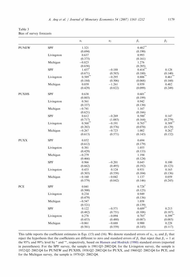
The bias adjustment occurs recursively, that is, we update the regression with new datapoints each quarter and re-estimate the coefficients.Table 3 provides empirical evidence regarding these biases using the full sample. For
each inflation measure, the first three rows report the results from regression (15). The SPFsurvey forecasts produce b1s that are smaller than one for all inflation measures, which are,with the exception of PUXX, significant at the 95% level. However, the point estimates ofa1 are also positive, although mostly not significant, which implies that at low levels ofinflation, the surveys under-predict future inflation and at high levels of inflation thesurveys over-predict future inflation. The turning point is 0:852=ð1� 0:694Þ ¼ 2:8%, sothat the SPF survey mostly over-predicts inflation. The Livingston and Michigan surveysproduce largely unbiased forecasts because the slope coefficients are insignificantlydifferent from one and the constants are insignificantly different from zero. Nevertheless,because the intercepts are positive (negative) for the Livingston (Michigan) survey, and theslope coefficients largely smaller (larger) than one, the Livingston (Michigan) survey tendsto produce mostly forecasts that are too low (high).Thomas (1999) and Mehra (2002) suggest that the bias in the survey forecasts may vary
across accelerating versus decelerating inflation environments, or across the business cycle.To take account of this possible asymmetry in the bias, we augment Eq. (15) with a dummyvariable, Dt, which equals one if inflation at time t exceeds its past two-year movingaverage,
pt �1
8
X7j¼0
pt�j40,
otherwise Dt is set equal to zero. The regression becomes
ptþ4;4 ¼ a1 þ a2Dt þ b1fSt þ b2Dtf
St þ �tþ4;4. (16)
We denote the survey forecasts that are non-linearly bias-adjusted using Eq. (16) as SPF3,LIV3, and MCH3 for the SPF, Livingston, and Michigan surveys, respectively.4
The bottom three rows of each panel in Table 3 report results from regression (16). Non-linear biases are reflected in significant a2 or b2 coefficients. For the SPF survey, there is nostatistical evidence of non-linear biases. For all inflation measures, the SPF’s negative a2and positive b2 coefficients indicates that accelerating inflation implies a smaller interceptand a higher slope coefficient, bringing the SPF forecasts closer to unbiasedness. For theMichigan survey, the biases are larger in magnitude (except for the PUXX measure) butthere is only one significant coefficient: accelerating inflation yields a significantly higherslope coefficient for the PUXHS measure. Economically, the Michigan survey is very closeto unbiasedness in decelerating inflation environments, but over- (under-) predicts futureinflation at low (high) inflation levels in accelerating inflation environments.
4We also examined bias adjustments using the change in annual inflation, using
ptþ4;4 � pt;4 ¼ a1 þ b1ðfSt � pt;4Þ þ �tþ4;4
in place of Eq. (15) and
ptþ4;4 � pt;4 ¼ a1 þ a2Dt þ b1ðfSt � pt;4Þ þ b2Dtðf
St � pt;4Þ þ �tþ4;4
in place of Eq. (16). Like the bias adjustments in Eqs. (15) and (16), these bias adjustments also do not outperform
the raw survey forecasts and generally perform worse than the bias adjustments using inflation levels.
ARTICLE IN PRESS
Table 3
Bias of survey forecasts
a1 a2 b1 b2
PUNEW SPF 1.321 0.482**
(0.694) (0.190)Livingston 0.637 0.993
(0.375) (0.161)Michigan �0.823 1.276
(0.658) (0.205)SPF 1.437* �0.188 0.414** 0.128
(0.671) (0.585) (0.180) (0.140)Livingston 0.589** �0.295 0.806** 0.461**
(0.184) (0.506) (0.068) (0.160)Michigan 0.039 �1.261 0.959 0.482
(0.429) (0.822) (0.099) (0.249)
PUXHS SPF 0.638 0.601*
(0.803) (0.199)Livingston 0.561 0.942
(0.337) (0.130)Michigan �0.741 1.167
(0.621) (0.166)SPF 0.612 �0.269 0.580* 0.147
(0.717) (1.085) (0.164) (0.279)Livingston 0.568** �0.191 0.765** 0.389**
(0.202) (0.576) (0.070) (0.129)Michigan �0.267 �0.723 1.002 0.262*
(0.613) (0.571) (0.143) (0.132)
PUXX SPF 0.852 0.694(0.612) (0.179)
Livingston 0.381 1.055(0.429) (0.133)
Michigan �0.279 1.194(0.466) (0.124)
SPF 0.966 �0.201 0.643 0.100(0.662) (0.495) (0.192) (0.123)
Livingston 0.433 0.124 0.931 0.165(0.303) (0.558) (0.104) (0.136)
Michigan �0.160 �0.042 1.137 0.059(0.579) (0.842) (0.146) (0.245)
PCE SPF 0.041 0.728*
(0.500) (0.125)Livingston 0.234 0.949
(0.479) (0.136)Michigan �0.547 1.058
(0.521) (0.139)SPF 0.122 �0.571 0.689** 0.213
(0.482) (0.751) (0.108) (0.187)Livingston 0.278 �0.094 0.785* 0.399**
(0.453) (0.480) (0.087) (0.085)Michigan �0.061 �0.688 0.900 0.228
(0.581) (0.559) (0.145) (0.117)
This table reports the coefficient estimates in Eqs. (15) and (16). We denote standard errors of a1, a2 and b2 thatreject the hypothesis that the coefficients are different to zero and standard errors of b1 that reject that b1 ¼ 1 at
the 95% and 99% level by � and ��, respectively, based on Hansen and Hodrick (1980) standard errors (reported
in parentheses). For the SPF survey, the sample is 1981:Q3–2002:Q4; for the Livingston survey, the sample is
1952:Q2–2002:Q4 for PUNEW and PUXHS, 1958:Q2–2002:Q4 for PUXX, and 1960:Q2–2002:Q4 for PCE; and
for the Michigan survey, the sample is 1978:Q1–2002:Q4.
A. Ang et al. / Journal of Monetary Economics 54 (2007) 1163–1212 1179
ARTICLE IN PRESSA. Ang et al. / Journal of Monetary Economics 54 (2007) 1163–12121180
The Livingston survey for which we have the longest data sample has the strongestevidence of non-linear bias. The coefficients have the same sign as for the other surveys,but now the b2 slope coefficients significantly increase in accelerating inflationenvironments for all inflation measures except PUXX. As in the case of the SPF survey,the Livingston survey is closer to being unbiased in accelerating inflation environments.Without accounting for non-linearity, the Livingston survey produces largely unbiasedforecasts in Table 3. However, the results of regression (16) for the Livingston survey showit produces mostly biased forecasts in decelerating inflation environments, under-predicting future inflation when inflation is relatively low, and over-predicting futureinflation when inflation is relatively high.
3.5. Assessing forecasting models
3.5.1. Out-of-sample periods
We select two starting dates for our out-of-sample forecasts, 1985:Q4 and 1995:Q4. Ourmain analysis focuses on recursive out-of-sample forecasts, which use all the data availableat time t to forecast annual future inflation from t to tþ 4. Hence, the windows usedfor estimation lengthen through time. We also consider out-of-sample forecasts with afixed rolling window. All of our annual forecasts are computed at a quarterly frequency,with the exception of forecasts from the Livingston survey, where forecasts are onlyavailable for the second and fourth quarter each year.5 The out-of-sample periods endin 2002:Q4, except for forecasts with the composite real activity factor, which end in2001:Q3.
3.5.2. Measuring forecast accuracy
We assess forecast accuracy with the RMSE of the forecasts produced by each modeland also report the ratio of RMSEs relative to a time-series ARMAð1; 1Þ benchmark thatuses only information in the past series of inflation. We show below that the ARMAð1; 1Þmodel nearly always produces the lowest RMSE among all of the ARIMA time-seriesmodels that we examine.To compare the out-of-sample forecasting performance of the various models, we
perform a forecast comparison regression, following Stock and Watson (1999):
ptþ4;4 ¼ lf ARMAt þ ð1� lÞf x
t þ �tþ4;4, (17)
where f ARMAt is the forecast of ptþ4;4 from the ARMAð1; 1Þ time-series model, f x
t is theforecast from the candidate model x, and �tþ4;4 is the forecast error associated withthe combined forecast. If l ¼ 0, then forecasts from the ARMAð1; 1Þ model add nothing tothe forecasts from candidate model x, and we thus conclude that model x out-performs theARMAð1; 1Þ benchmark. If l ¼ 1, then forecasts from model x add nothing to forecastsfrom the ARMAð1; 1Þ time-series benchmark.Stock and Watson (1999) note that inference about l is complicated by the fact that the
forecasts errors, �tþ4;4, follow a MA(3) process because the overlapping annualobservations are sampled at a quarterly frequency. We compute standard errors that
5While the RMSEs for the Livingston survey represent a different sample than those of all other models and
surveys, we also produced forecasts for a common semi-annual sample. The results are robust and we do not
further comment on them.
ARTICLE IN PRESSA. Ang et al. / Journal of Monetary Economics 54 (2007) 1163–1212 1181
account for the overlap by using Hansen and Hodrick (1980) standard errors. To also takeinto account the estimated parameter uncertainty in one or both sets of the forecasts,f ARMA
t and f xt , we also compute West (1996) standard errors. The appendix provides a
detailed description of the computations involved.
3.6. Combining models
A long statistics literature documents that forecast combinations typically provide betterforecasts than individual forecasting models.6 For inflation forecasts, Stock and Watson(1999) and Wright (2004), among others, show that combined forecasts using real activityand financial indicators are usually more accurate than individual forecasts. To examine ifcombining the information in different forecasts leads to gains in out-of-sample forecastingaccuracy, we examine five different methods of combining forecasts. All these methodsinvolve placing different weights on n individual forecasting models. The five modelcombination methods can be summarized as follows:
Combination methods
1.
6
Tim
Mean.
2. Median. 3. OLS. 4. Equal-weight prior. 5. Unit-weight prior.All our model combinations are ex ante. That is, we compute the weights on the modelsusing the history of out-of-sample forecasts up to time t. Hence, the ex ante methodassesses actual out-of-sample forecasting power of combination methods. For example, theweights used to construct the ex ante combined forecast at 2000:Q4 are based on aregression of realized annual inflation over 1985:Q4 to 2000:Q4 on the constructed out-of-sample forecasts over the same period.
In the first two model combination methods, we simply look at the overall mean andmedian, respectively, over n different forecasting models. Equal weighting of manyforecasts has been used as early as Bates and Granger (1969) and, in practice, simple equal-weighting forecasting schemes are hard to beat. In particular, Stock and Watson (2003)show that this method produces superior out-of-sample forecasts of inflation.
In the last three combination methods, we compute different individual model weightsthat vary over time. These weights are estimated as slope coefficients in a regression ofrealized inflation on model forecasts:
ptþ4;4 ¼Xn
i¼1
oit f i
t þ �t;tþ4; t ¼ 1; . . . ;T , (18)
where f it is the ith model forecast at time t. The n� 1 weight vector ot ¼ foi
tg is estimatedeither by OLS, as in our third model combination specification, or using the mixed
See the literature reviews by, among others, Clemen (1989), Diebold and Lopez (1996), and more recently
mermann (2006).
ARTICLE IN PRESSA. Ang et al. / Journal of Monetary Economics 54 (2007) 1163–12121182
regressor method proposed by Theil and Goldberger (1961) and Theil (1963), as incombination methods 4 and 5.To describe the last two combination methods, we set up some notation. Suppose we
have T forecast observations with n individual models. Let F be the T � n matrix offorecasts and p the T � 1 vector of actual future inflation levels that are being forecast.Consequently, the sth row of F is given by F s ¼ ff
1s ; . . . ; f
ns g. The mixed regression
estimator can be viewed as a Bayesian estimator with the prior o�Nðm; s2oIÞ, where s2o is ascalar and I the n� n identity matrix. The estimator can be derived as:
bo ¼ ðF 0F þ gIÞ�1ðF 0pþ gmÞ, (19)
where the parameter g controls the amount of shrinkage towards the prior. In particular,when g ¼ 0, the estimator simplifies to standard OLS, and when g!1, the estimatorapproaches the weighted average of the forecasts, with the weights given by the priorweights. It is instructive to re-write the estimator as a weighted average of the OLSestimator and the prior:bo ¼ yOLS oOLS þ yprior m
with yOLS ¼ ðF0F þ gIÞ�1ðF 0F Þ and yprior ¼ ðF 0F þ gIÞ�1ðgIÞ, so that the weights add up to
the identity matrix.We use empirical Bayes methods and estimate the shrinkage parameter as
bg ¼ bs2=bs2o, (20)
where
bs2 ¼ 1
Tp0½I � F ðF 0F Þ�1F 0�p
and
bs2o ¼ p0p� Tbs2traceðF 0F Þ
.
To interpret the shrinkage parameter, observe that bs2 is simply the residual variance of theregression; the numerator of bs2o is the fitted variance of the regression and the denominatoris the average variance of the independent variables (the forecasts) in the regression.Consequently, the shrinkage parameter, g, in Eq. (20) increases when the variance of theindependent variables becomes larger, and decreases as the R2 of the regression increases.In other words, if forecasts are (not) very variable and the regression R2 is small (large), wetrust the prior (the regression).We examine the effect of two priors. In model combination 4, we use an equal-weight
prior where each element of m, mi ¼ 1=n; i ¼ 1; . . . ; n, which leads to the Ridge regressorused by Stock and Watson (1999). In the second prior (model combination 5), we assignunit weight to one type of forecast, for example, m ¼ f0 . . . 1 . . . 0g0. One natural choice fora unit weight prior would be to choose the best performing univariate forecast model.When we compute the model weights, we impose the constraint that the weight on each
model is positive and the weights sum to one. This ensures that the weights represent thebest combination of models that produce good forecasts in their own right, rather thanplace negative weights on models that give consistently wrong forecasts. This is also verysimilar to shrinkage methods of forecasting (see Stock and Watson, 2005). For example,
ARTICLE IN PRESSA. Ang et al. / Journal of Monetary Economics 54 (2007) 1163–1212 1183
Bayesian model averaging uses posterior probabilities as weights, which are, byconstruction, positive and sum to one.7
The positivity constraint is imposed by minimizing the usual loss function, L, associatedwith OLS for combination method 3:
L ¼ ðp� FoÞ0ðp� FoÞ,
and a loss function for the mixed regressor estimations (combination methods 4 and 5):
L ¼ðp� FoÞ0ðp� FoÞbs2 þ
ðo� mÞ0ðo� mÞbs2o ,
subject to the positivity constraints. These are standard constrained quadratic program-ming problems.
4. Empirical results
Section 4.1 lays out our main empirical results for the forecasts of time-series models,OLS Phillips curve regressions, term structure models, and survey forecasts. Wesummarize these results in Section 4.2. Section 4.3 investigates how consistently the bestmodels perform through time and Section 4.4 considers the effect of rolling windows.Section 4.5 reports the results of combining model forecasts.
4.1. Forecast accuracy
4.1.1. Time-series models
In Table 4, we report RMSE statistics, in annual percentage terms, for the ARIMAmodel out-of-sample forecasts over the post-1985 and post-1995 periods. The ARIMARMSEs generally range from around 0.4–0.7% for PUXX to around 1.4–2.2% forPUXHS. For the post-1985 sample, the ARMAð1; 1Þ model generates the lowest RMSEamong all ARIMA models in forecasting PUNEW and PUXHS, but the annualAtkeson–Ohanian (2001) random walk is superior in forecasting core inflation (PUXX)and PCE. As the best quarterly ARIMA model, we select the ARMAð1; 1Þ model as thebenchmark for the remainder of the paper.8 In the post-1995 period, it beats both thequarterly RW and AR models in forecasting the PUXHS and PCE measure, but the ARmodel has a lower RMSE in forecasting PUNEW and PUXX, whereas the quarterly RWgenerates a lower RMSE in forecasting PUXX . Yet, the improvements are minor and theARMAð1; 1Þ model remains overall best among the three quarterly ARIMA models.However, the annual random walk is the best forecasting model for PUXX and PCE. Itbeats the ARMAð1; 1Þ model for three of the four inflation measures and generates a muchlower RMSE for forecasting core inflation (PUXX).
Table 4 also reports the RMSEs of the non-linear regime-switching model, RGM. Overthe post-1985 period, RGM generally performs in line with, and slightly worse than, a
7Diebold (1989) shows that when the target is persistent, as in the case of inflation, the forecast error from the
combination regression will typically be serially correlated and hence predictable, unless the constraint that the
weights sum to one is imposed.8The estimated ARMA models contain large autoregressive roots with negative MA roots. As Ng and Perron
(2001) comment, the negative MA components lead unit root tests to over-reject the null of non-stationarity.

ARTICLE IN PRESS
Table 4
Time-series forecasts of annual inflation
Post-1985 sample Post-1995 sample
RMSE ARMA ¼ 1 RMSE ARMA ¼ 1
PUNEW ARMA 1.136 1.000 1.144 1.000
AR 1.140 1.003 1.130 0.988
RGM 1.420 1.250 0.873 0.764
AORW 1.177 1.036 1.128 0.986
RW 1.626 1.431 1.529 1.337
PUXHS ARMA 1.490 1.000 1.626 1.000
AR 1.515 1.017 1.634 1.005
RGM 1.591 1.068 1.355 0.833
AORW 1.580 1.061 1.670 1.027
RW 2.172 1.458 2.146 1.320
PUXX ARMA 0.630 1.000 0.600 1.000
AR 0.644 1.023 0.593 0.988
RGM 0.677 1.075 0.727 1.211
AORW 0.516 0.819 0.372 0.620
RW 0.675 1.072 0.549 0.915
PCE ARMA 0.878 1.000 0.944 1.000
AR 0.942 1.073 1.014 1.074
RGM 0.945 1.077 1.081 1.145
AORW 0.829 0.945 0.869 0.921
RW 1.140 1.298 1.215 1.288
We forecast annual inflation out-of-sample from 1985:Q4 to 2002:Q4 and from 1995:Q4 to 2002:Q4 at a quarterly
frequency. Table 2 contains full details of the time-series models. Numbers in the RMSE columns are reported in
annual percentage terms. The column labeled ARMA ¼ 1 reports the ratio of the RMSE relative to the
ARMAð1; 1Þ specification.
A. Ang et al. / Journal of Monetary Economics 54 (2007) 1163–12121184
standard ARMA model. There is some evidence that non-linearities are important forforecasting in the post-1995 sample, where the regime-switching model outperforms all theARIMA models in forecasting PUNEW and PUXHS. Both these inflation series becomemuch less persistent post-1995, and the RGM model captures this by transitioning to aregime of less persistent inflation. However, the Hamilton (1989) RGM model performsworse than a linear ARMA model for forecasting PUXX and PCE.
4.1.2. OLS Phillips curve forecasts
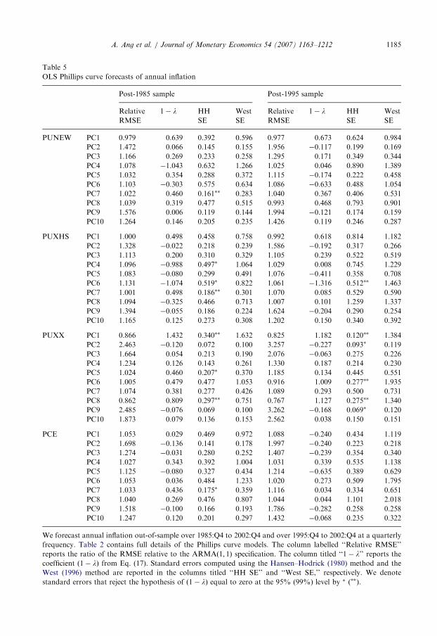
Table 5 reports the out-of-sample RMSEs and the model comparison regressionestimates (Eq. (17)) for the Phillips curve models described in Section 3.2, relative to thebenchmark of the ARMAð1; 1Þ model. The overall picture in Table 5 is that theARMAð1; 1Þ model typically outperforms the Phillips curve forecasts. Of the 80comparisons (10 models, two out-samples, and four inflation measures), the modelcomparison regression coefficient ð1� lÞ is not significantly positive at the 95% level inany of 80 cases using West (1996) standard errors! It must be said that the coefficients aresometimes positive and far away from zero, but the standard errors are generally ratherlarge. When we compute Hansen–Hodrick (1980) standard errors, we still only obtain 14
ARTICLE IN PRESS
Table 5
OLS Phillips curve forecasts of annual inflation
Post-1985 sample Post-1995 sample
Relative 1� l HH West Relative 1� l HH West
RMSE SE SE RMSE SE SE
PUNEW PC1 0.979 0.639 0.392 0.596 0.977 0.673 0.624 0.984
PC2 1.472 0.066 0.145 0.155 1.956 �0.117 0.199 0.169
PC3 1.166 0.269 0.233 0.258 1.295 0.171 0.349 0.344
PC4 1.078 �1.043 0.632 1.266 1.025 0.046 0.890 1.389
PC5 1.032 0.354 0.288 0.372 1.115 �0.174 0.222 0.458
PC6 1.103 �0.303 0.575 0.634 1.086 �0.633 0.488 1.054
PC7 1.022 0.460 0:161�� 0.283 1.040 0.367 0.406 0.531
PC8 1.039 0.319 0.477 0.515 0.993 0.468 0.793 0.901
PC9 1.576 0.006 0.119 0.144 1.994 �0.121 0.174 0.159
PC10 1.264 0.146 0.205 0.235 1.426 0.119 0.246 0.287
PUXHS PC1 1.000 0.498 0.458 0.758 0.992 0.618 0.814 1.182
PC2 1.328 �0.022 0.218 0.239 1.586 �0.192 0.317 0.266
PC3 1.113 0.200 0.310 0.329 1.105 0.239 0.522 0.519
PC4 1.096 �0.988 0:497� 1.064 1.029 0.008 0.745 1.229
PC5 1.083 �0.080 0.299 0.491 1.076 �0.411 0.358 0.708
PC6 1.131 �1.074 0:519� 0.822 1.061 �1.316 0:512�� 1.463
PC7 1.001 0.498 0:186�� 0.301 1.070 0.085 0.529 0.590
PC8 1.094 �0.325 0.466 0.713 1.007 0.101 1.259 1.337
PC9 1.394 �0.055 0.186 0.224 1.624 �0.204 0.290 0.254
PC10 1.165 0.125 0.273 0.308 1.202 0.150 0.340 0.392
PUXX PC1 0.866 1.432 0:340�� 1.632 0.825 1.182 0:120�� 1.384
PC2 2.463 �0.120 0.072 0.100 3.257 �0.227 0:093� 0.119
PC3 1.664 0.054 0.213 0.190 2.076 �0.063 0.275 0.226
PC4 1.234 0.126 0.143 0.261 1.330 0.187 0.214 0.230
PC5 1.024 0.460 0:207� 0.370 1.185 0.134 0.445 0.551
PC6 1.005 0.479 0.477 1.053 0.916 1.009 0:277�� 1.935
PC7 1.074 0.381 0.277 0.426 1.089 0.293 0.500 0.731
PC8 0.862 0.809 0:297�� 0.751 0.767 1.127 0:275�� 1.340
PC9 2.485 �0.076 0.069 0.100 3.262 �0.168 0:069� 0.120
PC10 1.873 0.079 0.136 0.153 2.562 0.038 0.150 0.151
PCE PC1 1.053 0.029 0.469 0.972 1.088 �0.240 0.434 1.119
PC2 1.698 �0.136 0.141 0.178 1.997 �0.240 0.223 0.218
PC3 1.274 �0.031 0.280 0.252 1.407 �0.239 0.354 0.340
PC4 1.027 0.343 0.392 1.004 1.031 0.339 0.535 1.138
PC5 1.125 �0.080 0.327 0.434 1.214 �0.635 0.389 0.629
PC6 1.053 0.036 0.484 1.233 1.020 0.273 0.509 1.795
PC7 1.033 0.436 0:175� 0.359 1.116 0.034 0.334 0.651
PC8 1.040 0.269 0.476 0.807 1.044 0.044 1.101 2.018
PC9 1.518 �0.100 0.166 0.193 1.786 �0.282 0.258 0.258
PC10 1.247 0.120 0.201 0.297 1.432 �0.068 0.235 0.322
We forecast annual inflation out-of-sample over 1985:Q4 to 2002:Q4 and over 1995:Q4 to 2002:Q4 at a quarterly
frequency. Table 2 contains full details of the Phillips curve models. The column labelled ‘‘Relative RMSE’’
reports the ratio of the RMSE relative to the ARMAð1; 1Þ specification. The column titled ‘‘1� l’’ reports thecoefficient ð1� lÞ from Eq. (17). Standard errors computed using the Hansen–Hodrick (1980) method and the
West (1996) method are reported in the columns titled ‘‘HH SE’’ and ‘‘West SE,’’ respectively. We denote
standard errors that reject the hypothesis of ð1� lÞ equal to zero at the 95% (99%) level by � ð��Þ.
A. Ang et al. / Journal of Monetary Economics 54 (2007) 1163–1212 1185
ARTICLE IN PRESSA. Ang et al. / Journal of Monetary Economics 54 (2007) 1163–12121186
cases of significant ð1� lÞ coefficients with p-values less than 5%, and of these 14 cases,only nine are positive.The OLS Phillips curve regressions are most successful in forecasting core inflation,
PUXX. Of the nine cases where the Phillips curve produces lower RMSEs than theARMAð1; 1Þmodel, five occur for PUXX. The best model forecasting PUXX inflation usesthe composite Bernanke–Boivin–Eliasz aggregate real activity factor (PC8). While theð1� lÞ coefficients are large for PC8, their West (1996) standard errors are also large, sothey are insignificant for both samples. Another relatively successful Phillips curvespecification is the PC7 model that uses the Stock–Watson non-financial experimentalleading index-2. This index does not embed asset pricing information. PC7 for PUXHSpost-1985 is the only case, out of 80 cases, that generates a positive ð1� lÞ coefficientwhich is significant at a level higher than the 90% level using West standard errors, but itsperformance deteriorates for the post-1995 sample. All of the RMSEs of PC7 are alsohigher than the RMSE of an ARMAð1; 1Þ model. In contrast, the PC1 model, whichsimply uses past inflation and past GDP growth, delivers five of the nine relative RMSEsbelow one and beats PC7 in all but one case.Among the various Phillips curve models, it is also striking that the PC4 model
consistently beats the PC2 and PC3 models, sometimes by a wide margin in terms ofRMSE. The PC2 and PC3 models use detrended measures of output that are often used toproxy for the output gap. PC4 uses the labor share as a real activity measure, whichis sometimes used as a proxy for the marginal cost concept in New Keynesian models.This is interesting because the recent Phillips curve literature (see Gali and Gertler,1999) stresses that marginal cost measures provide a better characterization of (in-sample)inflation dynamics than detrended output measures. Our results suggest that the useof marginal cost measures also leads to better out-of-sample predictive power. However,the use of GDP growth leads to significantly better forecasts than the labor share measure,but GDP growth remains, so far, conspicuously absent in the recent Phillips curveliterature.Finally, using Table 4 together with Table 5, it is easy to verify whether the
Atkeson–Ohanian (2001) results hold up for our models and data. Essentially, they do: theannual random walk beats the Phillips curve models in 72 out of 80 cases. All the caseswhere a Phillips curve model beats the annual random walk occur in forecasting thePUNEW or PUXHS measures.
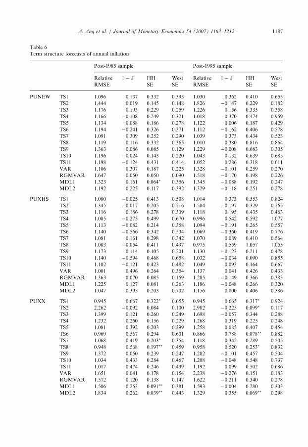
4.1.3. Term structure forecasts
In Table 6, we report the out-of-sample forecasting results for the various term structuremodels (see Section 3.3). Generally, the term structure based forecasts perform worse thanthe Phillips-curve based forecasts. Over a total of 120 statistics (15 models, four inflationmeasures, two sample periods), term structure based-models beat the ARMAð1; 1Þ modelin only eight cases in terms of producing smaller RMSE statistics. The ð1� lÞ coefficientsare usually positive for forecasting PUXX in the post-1985 period, but half are negative inthe post-1995 sample. Unfortunately, the use of West (1996) standard errors turns 10 casesof significantly positive ð1� lÞ coefficients using Hansen–Hodrick (1980) standard errorsinto insignificant coefficients. The performance of the term structure forecasts is so poorthat using West (1996) standard errors, in none of the 120 cases are the ð1� lÞ parameterssignificant at the 95% level. This may be caused by many of the term structure models,especially the no-arbitrage models, having relatively large numbers of parameters.
ARTICLE IN PRESS
Table 6
Term structure forecasts of annual inflation
Post-1985 sample Post-1995 sample
Relative 1� l HH West Relative 1� l HH West
RMSE SE SE RMSE SE SE
PUNEW TS1 1.096 0.137 0.332 0.393 1.030 0.362 0.410 0.653
TS2 1.444 0.019 0.145 0.148 1.826 �0.147 0.229 0.182
TS3 1.176 0.193 0.229 0.259 1.226 0.156 0.335 0.358
TS4 1.166 �0.108 0.249 0.321 1.018 0.370 0.474 0.959
TS5 1.134 0.088 0.186 0.278 1.122 0.006 0.187 0.429
TS6 1.194 �0.241 0.326 0.371 1.112 �0.162 0.406 0.578
TS7 1.091 0.309 0.252 0.290 1.039 0.373 0.434 0.523
TS8 1.119 0.116 0.332 0.365 1.010 0.380 0.816 0.864
TS9 1.363 0.086 0.085 0.129 1.229 �0.008 0.083 0.305
TS10 1.196 �0.024 0.143 0.220 1.043 0.132 0.639 0.685
TS11 1.198 �0.124 0.431 0.414 1.052 0.286 0.318 0.611
VAR 1.106 0.307 0.187 0.225 1.328 �0.101 0.259 0.270
RGMVAR 1.647 0.050 0.050 0.090 1.518 �0.170 0.198 0.226
MDL1 1.323 0.161 0:064� 0.356 1.345 �0.088 0.192 0.247
MDL2 1.192 0.225 0.117 0.392 1.329 �0.118 0.251 0.278
PUXHS TS1 1.080 �0.025 0.413 0.508 1.014 0.373 0.553 0.824
TS2 1.345 �0.017 0.205 0.216 1.584 �0.197 0.329 0.265
TS3 1.116 0.186 0.278 0.309 1.118 0.195 0.435 0.463
TS4 1.085 �0.275 0.499 0.670 0.996 0.542 0.592 1.077
TS5 1.113 �0.082 0.214 0.358 1.094 �0.191 0.265 0.557
TS6 1.140 �0.566 0.342 0.534 1.069 �0.360 0.419 0.776
TS7 1.081 0.161 0.298 0.342 1.070 0.089 0.410 0.564
TS8 1.083 �0.054 0.411 0.497 0.975 0.559 1.057 1.055
TS9 1.173 0.114 0.105 0.201 1.130 �0.123 0.211 0.478
TS10 1.140 �0.594 0.468 0.658 1.032 �0.034 0.090 0.855
TS11 1.102 �0.121 0.423 0.482 1.049 0.093 0.164 0.667
VAR 1.001 0.496 0.264 0.354 1.137 0.041 0.426 0.433
RGMVAR 1.363 0.070 0.085 0.159 1.285 �0.149 0.366 0.383
MDL1 1.225 0.127 0.081 0.263 1.186 �0.048 0.266 0.320
MDL2 1.047 0.395 0.203 0.702 1.156 0.000 0.406 0.386
PUXX TS1 0.945 0.667 0:322� 0.655 0.945 0.665 0:317� 0.924
TS2 2.262 �0.092 0.084 0.100 2.982 �0.225 0:099� 0.117
TS3 1.399 0.121 0.260 0.249 1.698 �0.057 0.344 0.288
TS4 1.232 0.260 0.156 0.229 1.268 0.319 0.225 0.248
TS5 1.081 0.392 0.203 0.299 1.258 0.085 0.407 0.454
TS6 0.969 0.567 0.294 0.601 0.866 0.788 0:078�� 0.882
TS7 1.068 0.419 0:203� 0.354 1.118 0.342 0.289 0.505
TS8 0.948 0.568 0:197�� 0.459 0.958 0.520 0:253� 0.832
TS9 1.372 0.050 0.239 0.247 1.282 �0.101 0.457 0.504
TS10 1.034 0.433 0.284 0.467 1.208 �0.048 0.548 0.737
TS11 1.017 0.474 0.246 0.439 1.192 0.099 0.502 0.686
VAR 1.651 0.041 0.178 0.154 2.238 �0.276 0.151 0.183
RGMVAR 1.572 0.120 0.138 0.147 1.622 �0.211 0.340 0.278
MDL1 1.506 0.253 0:091�� 0.381 1.593 �0.004 0.280 0.303
MDL2 1.834 0.262 0:039�� 0.443 1.329 0.355 0:069�� 0.298
A. Ang et al. / Journal of Monetary Economics 54 (2007) 1163–1212 1187
ARTICLE IN PRESS
Table 6 (continued )
Post-1985 sample Post-1995 sample
Relative 1� l HH West Relative 1� l HH West
RMSE SE SE RMSE SE SE
PCE TS1 1.075 �0.073 0.453 0.847 1.078 �0.207 0.433 1.192
TS2 1.670 �0.149 0.145 0.181 1.966 �0.247 0.226 0.221
TS3 1.279 �0.053 0.288 0.259 1.373 �0.245 0.376 0.360
TS4 1.075 0.018 0.372 0.864 1.059 0.234 0.442 0.816
TS5 1.126 �0.115 0.331 0.456 1.202 �0.645 0.383 0.663
TS6 1.094 �0.149 0.428 0.896 1.100 �0.358 0.397 1.322
TS7 1.018 0.443 0.271 0.481 1.106 0.033 0.303 0.673
TS8 1.027 0.374 0.414 0.720 1.025 0.346 1.058 1.855
TS9 1.141 �0.024 0.192 0.304 1.121 �0.825 0.584 0.939
TS10 1.087 �0.569 0.549 0.992 1.110 �0.850 0.638 1.177
TS11 1.086 0.006 0.418 0.665 1.132 �0.396 0.288 0.878
VAR 1.286 �0.179 0.274 0.298 1.511 �0.337 0.392 0.327
RGMVAR 1.507 �0.242 0.131 0.237 1.461 �0.356 0.233 0.424
MDL1 1.169 0.144 0.235 0.432 1.271 �0.374 0.284 0.481
MDL2 1.314 �0.205 0.159 1.220 1.339 �0.331 0:120�� 0.589
We forecast annual inflation out-of-sample over 1985:Q4–2002:Q4 and over 1995:Q4–2002:Q4 at a quarterly
frequency. Table 2 contains full details of the term structure models. The column labelled ‘‘Relative RMSE’’
reports the ratio of the RMSE relative to the ARMAð1; 1Þ specification. The column titled ‘‘1� l’’ reports thecoefficient ð1� lÞ from Eq. (17). Standard errors computed using the Hansen–Hodrick (1980) method and the
West (1996) method are reported in the columns titled ‘‘HH SE’’ and ‘‘West SE,’’ respectively. We denote
standard errors that reject the hypothesis of ð1� lÞ equal to zero at the 95% (99%) level by � ð��Þ.
A. Ang et al. / Journal of Monetary Economics 54 (2007) 1163–12121188
The term structure models most successfully forecast core inflation, PUXX, whichdelivers six of the eight cases with smaller RMSEs than an ARMAð1; 1Þ model. Inparticular, the TS1 model that includes inflation, GDP growth, and the short rate beats anARMAð1; 1Þ model and has a positive ð1� lÞ, but insignificant, coefficient in both thepost-1985 and post-1995 samples. The other models with term structure information thatare successful at forecasting PUXX are TS6 and TS8, both of which also include short rateinformation.The finance literature has typically used term spreads, not short rates, to predict future
inflation changes (see, for example, Mishkin, 1990, 1991). In contrast to the relative successof the models with short rate information, models TS9–TS11, which incorporateinformation from the term spread, perform badly. They produce higher RMSE statisticsthan the benchmark ARMAð1; 1Þ model for all four inflation measures. This is consistentwith Estrella and Mishkin (1997) and Kozicki (1997), who find that the forecasting abilityof the term spread is diminished after controlling for lagged inflation. However, we showthat the short rate still contains modest predictive power even after controlling for laggedinflation. Thus, the short rate, not the term spread, contains the most predictive power insimple forecasting regressions.Table 6 shows that the performance of iterated VAR forecasts is mixed. VARs produce
lower RMSEs than ARMAð1; 1Þ models. The relatively poor performance of long-horizonVAR forecasts for inflation contrasts with the good performance for VARs in forecastingGDP (see Ang et al., 2006a) and for forecasting other macroeconomic time series
ARTICLE IN PRESSA. Ang et al. / Journal of Monetary Economics 54 (2007) 1163–1212 1189
(see Marcellino et al., 2006). The non-linear empirical regime-switching VAR (RGMVAR)generally fares worse than the VAR. This result stands in contrast to the relatively strongperformance of the univariate regime-switching model using only inflation data (RGM inTable 4) for forecasting PUNEW and PUXX. This implies that the non-linearities in termstructure data have no marginal value for forecasting inflation above the non-linearitiesalready present in inflation itself.
The last two lines of each panel in Table 6 shows that there is some evidence that no-arbitrage forecasts (MDL1-2) are useful for forecasting PUXX in the post-1985 sample.While the ð1� lÞ coefficients are significant using Hansen–Hodrick (1980) standard errors,they are not significant with West (1996) standard errors. Moreover, both no-arbitrageterm structure models always fail to beat the ARMAð1; 1Þ forecasts in terms of RMSE.While the finance literature shows that inflation is a very important determinant of yieldcurve movements, our results show that the no-arbitrage cross-section of yields appears toprovide little marginal forecasting ability for the dynamics of future inflation over simpletime-series models.
4.1.4. Surveys
Table 7 reports the results for the survey forecasts and reveals several notable results.First, surveys perform very well in forecasting PUNEW, PUXHS, and PUXX. With onlyone exception, the raw survey forecasts SPF1, LIV1 and MICH1 have lower RMSEs thanARMAð1; 1Þ forecasts over both the post-1985 and the post-1995 samples (the exception isMICH1 for PUXX over the post-1985 sample). For example, for the post-1985 (post-1995)sample, the RMSE ratio of the raw SPF forecasts relative to an ARMAð1; 1Þ is 0.779(0.861) when predicting PUNEW. The horse races always assign large, positive ð1� lÞweights to the pure survey forecasts (the lowest one is 0.383) in both out-of-sample periods.Ignoring parameter uncertainty, the coefficients are significantly different from zero inevery case, but taking into account parameter uncertainty, statistical significancedisappears for the post-1995 samples, and in the case of the PUXX measure, even forthe post-1985 sample. This is true for all three surveys.
Second, while the SPF and Livingston surveys do a good job at forecasting all threemeasures of CPI inflation (PUNEW, PUXHS, and PUXX) out-of-sample, the Michigansurvey is relatively unsuccessful at forecasting core inflation, PUXX. It is not surprisingthat consumers in the Michigan survey fail to forecast PUXX, since PUXX excludes foodand energy which are integral components of the consumer’s basket of goods. Note thatwhile the annual PUNEW and PUXHS measures have the highest correlations with eachother (99% in both out-samples), core inflation is less correlated with the other CPImeasures. In particular, Table 1 reports that post-1995, the correlation of quarterly PUXXwith quarterly PUNEW (PUXHS) is only 33% (21%). Surveys do less well at forecastingPCE inflation, always producing worse forecasts in terms of RMSE than an ARMAð1; 1Þ.This result is expected because the survey participants are asked to forecast CPI inflation,rather than the consumption deflator PCE.
Third, the raw survey forecasts outperform the linear or non-linear bias adjustedforecasts (with the only notable exception being the bias-adjusted forecasts for PCE). As aspecific example, for PUNEW, the relative RMSE ratios are always higher for the modelswith suffix 2 (linear bias adjustment) or the models with suffix 3 (non-linear biasadjustment) compared to the raw survey forecasts across all three surveys. This resultis perhaps not surprising given the mixed evidence regarding biases in the survey data
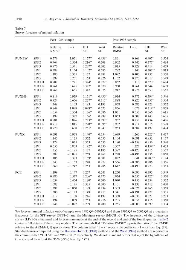
ARTICLE IN PRESS
Table 7
Survey forecasts of annual inflation
Post-1985 sample Post-1995 sample
Relative 1� l HH West Relative 1� l HH West
RMSE SE SE RMSE SE SE
PUNEW SPF1 0.779 1.051 0:177�� 0:439� 0.861 0.869 0:407� 0.554
SPF2 0.964 0.564 0:216�� 0.308 0.902 0.745 0:377� 0.484
SPF3 0.976 0.541 0:207�� 0.302 0.915 0.728 0.414 0.479
LIV1 0.789 1.164 0:102�� 0.585 0.792 1.140 0:203�� 0.913
LIV2 1.180 0.335 0.177 0.281 1.092 0.403 0.437 0.550
LIV3 1.299 0.251 0.163 0.226 1.152 0.275 0.517 0.549
MICH1 0.902 0.771 0:324� 0:379� 0.862 1.113 0:520� 0.684
MICH2 0.961 0.675 0:327� 0.370 0.930 0.861 0.644 0.609
MICH3 0.968 0.655 0.347 0.375 0.947 0.776 0.653 0.567
PUXHS SPF1 0.819 0.939 0:171�� 0:430� 0.914 0.773 0:394� 0.546
SPF2 0.924 0.666 0:227�� 0:312� 0.888 0.825 0:357� 0.504
SPF3 1.348 0.103 0.183 0.193 0.958 0.582 0.323 0.362
LIV1 0.844 1.098 0:099�� 0.573 0.856 1.072 0:214�� 0.878
LIV2 1.054 0.554 0:176�� 0.386 1.031 0.550 0.366 0.615
LIV3 1.199 0.327 0:156� 0.299 1.053 0.502 0.443 0.605
MICH1 0.881 0.876 0:273�� 0:398� 0.937 0.750 0.434 0.476
MICH2 0.918 0.815 0:290�� 0:395� 0.932 0.814 0.515 0.528
MICH3 0.970 0.608 0:251� 0.347 0.953 0.684 0.492 0.474
PUXX SPF1 0.691 0.968 0:140�� 0.654 0.699 1.260 0:225�� 1.437
SPF2 1.145 0.125 0.362 0.555 1.104 0.091 0.852 1.177
SPF3 1.179 0.035 0.373 0.555 1.180 �0.358 0.956 1.390
LIV1 0.655 0.803 0:192�� 0.730 0.557 1.227 0:134�� 1.453
LIV2 1.355 �0.185 0.177 0.185 1.387 �0.423 0.415 0.557
LIV3 1.289 �0.095 0.259 0.262 1.278 �0.496 0.735 0.850
MICH1 1.185 0.383 0:159� 0.301 0.822 1.041 0:208�� 2.124
MICH2 1.343 �0.153 0.248 0.272 1.566 �0.385 0.286 0.356
MICH3 1.360 �0.242 0.253 0.285 1.617 �0.493 0.273 0.363
PCE SPF1 1.199 0.147 0.267 0.241 1.250 0.090 0.395 0.349
SPF2 0.980 0.537 0:206�� 0.375 0.924 0.655 0:325� 0.570
SPF3 1.034 0.454 0:180� 0.306 1.040 0.453 0.234 0.362
LIV1 1.082 0.175 0.325 0.300 1.101 0.132 0.412 0.400
LIV2 1.397 �0.050 0.189 0.234 1.303 �0.026 0.265 0.358
LIV3 1.380 �0.123 0.149 0.212 1.341 �0.191 0.272 0.375
MICH1 1.217 0.108 0.216 0.192 1.338 �0.030 0.327 0.283
MICH2 1.194 0.039 0.253 0.216 1.205 0.056 0.415 0.350
MICH3 1.248 �0.022 0.239 0.200 1.255 �0.003 0.399 0.334
We forecast annual inflation out-of-sample over 1985:Q4–2002:Q4 and from 1995:Q4 to 2002:Q4 at a quarterly
frequency for the SPF survey (SPF1–3) and the Michigan survey (MICH1-3). The frequency of the Livingston
survey (LIV1-3) is biannual and forecasts are made at the end of the second and end of the fourth quarter. Table 2
contains full details of the survey models. The column labelled ‘‘Relative RMSE’’ reports the ratio of the RMSE
relative to the ARMAð1; 1Þ specification. The column titled ‘‘1� l’’ reports the coefficient ð1� lÞ from Eq. (17).
Standard errors computed using the Hansen–Hodrick (1980) method and the West (1996) method are reported in
the columns titled ‘‘HH SE’’ and ‘‘West SE,’’ respectively. We denote standard errors that reject the hypothesis of
ð1� lÞ equal to zero at the 95% (99%) level by � ð��Þ.
A. Ang et al. / Journal of Monetary Economics 54 (2007) 1163–12121190
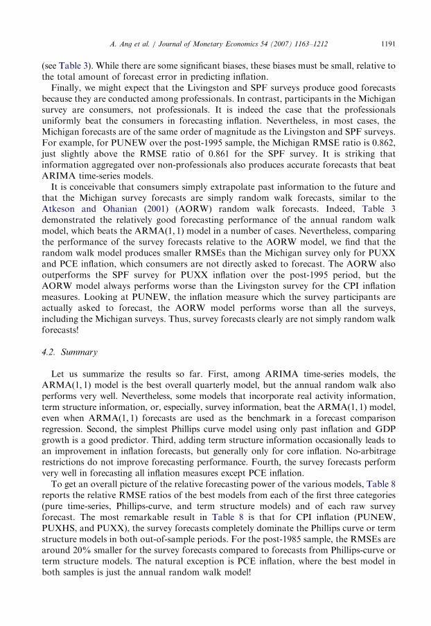
ARTICLE IN PRESSA. Ang et al. / Journal of Monetary Economics 54 (2007) 1163–1212 1191
(see Table 3). While there are some significant biases, these biases must be small, relative tothe total amount of forecast error in predicting inflation.
Finally, we might expect that the Livingston and SPF surveys produce good forecastsbecause they are conducted among professionals. In contrast, participants in the Michigansurvey are consumers, not professionals. It is indeed the case that the professionalsuniformly beat the consumers in forecasting inflation. Nevertheless, in most cases, theMichigan forecasts are of the same order of magnitude as the Livingston and SPF surveys.For example, for PUNEW over the post-1995 sample, the Michigan RMSE ratio is 0.862,just slightly above the RMSE ratio of 0.861 for the SPF survey. It is striking thatinformation aggregated over non-professionals also produces accurate forecasts that beatARIMA time-series models.
It is conceivable that consumers simply extrapolate past information to the future andthat the Michigan survey forecasts are simply random walk forecasts, similar to theAtkeson and Ohanian (2001) (AORW) random walk forecasts. Indeed, Table 3demonstrated the relatively good forecasting performance of the annual random walkmodel, which beats the ARMAð1; 1Þ model in a number of cases. Nevertheless, comparingthe performance of the survey forecasts relative to the AORW model, we find that therandom walk model produces smaller RMSEs than the Michigan survey only for PUXXand PCE inflation, which consumers are not directly asked to forecast. The AORW alsooutperforms the SPF survey for PUXX inflation over the post-1995 period, but theAORW model always performs worse than the Livingston survey for the CPI inflationmeasures. Looking at PUNEW, the inflation measure which the survey participants areactually asked to forecast, the AORW model performs worse than all the surveys,including the Michigan surveys. Thus, survey forecasts clearly are not simply random walkforecasts!
4.2. Summary
Let us summarize the results so far. First, among ARIMA time-series models, theARMAð1; 1Þ model is the best overall quarterly model, but the annual random walk alsoperforms very well. Nevertheless, some models that incorporate real activity information,term structure information, or, especially, survey information, beat the ARMAð1; 1Þ model,even when ARMAð1; 1Þ forecasts are used as the benchmark in a forecast comparisonregression. Second, the simplest Phillips curve model using only past inflation and GDPgrowth is a good predictor. Third, adding term structure information occasionally leads toan improvement in inflation forecasts, but generally only for core inflation. No-arbitragerestrictions do not improve forecasting performance. Fourth, the survey forecasts performvery well in forecasting all inflation measures except PCE inflation.
To get an overall picture of the relative forecasting power of the various models, Table 8reports the relative RMSE ratios of the best models from each of the first three categories(pure time-series, Phillips-curve, and term structure models) and of each raw surveyforecast. The most remarkable result in Table 8 is that for CPI inflation (PUNEW,PUXHS, and PUXX), the survey forecasts completely dominate the Phillips curve or termstructure models in both out-of-sample periods. For the post-1985 sample, the RMSEs arearound 20% smaller for the survey forecasts compared to forecasts from Phillips-curve orterm structure models. The natural exception is PCE inflation, where the best model inboth samples is just the annual random walk model!
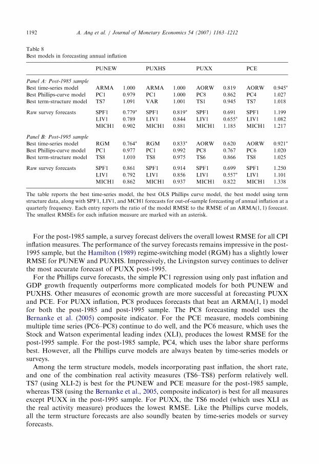
ARTICLE IN PRESS
Table 8
Best models in forecasting annual inflation
PUNEW PUXHS PUXX PCE
Panel A: Post-1985 sample
Best time-series model ARMA 1.000 ARMA 1.000 AORW 0.819 AORW 0:945�
Best Phillips-curve model PC1 0.979 PC1 1.000 PC8 0.862 PC4 1.027
Best term-structure model TS7 1.091 VAR 1.001 TS1 0.945 TS7 1.018
Raw survey forecasts SPF1 0:779� SPF1 0:819� SPF1 0.691 SPF1 1.199
LIV1 0.789 LIV1 0.844 LIV1 0:655� LIV1 1.082
MICH1 0.902 MICH1 0.881 MICH1 1.185 MICH1 1.217
Panel B: Post-1995 sample
Best time-series model RGM 0:764� RGM 0:833� AORW 0.620 AORW 0:921�
Best Phillips-curve model PC1 0.977 PC1 0.992 PC8 0.767 PC6 1.020
Best term-structure model TS8 1.010 TS8 0.975 TS6 0.866 TS8 1.025
Raw survey forecasts SPF1 0.861 SPF1 0.914 SPF1 0.699 SPF1 1.250
LIV1 0.792 LIV1 0.856 LIV1 0:557� LIV1 1.101
MICH1 0.862 MICH1 0.937 MICH1 0.822 MICH1 1.338
The table reports the best time-series model, the best OLS Phillips curve model, the best model using term
structure data, along with SPF1, LIV1, and MCH1 forecasts for out-of-sample forecasting of annual inflation at a
quarterly frequency. Each entry reports the ratio of the model RMSE to the RMSE of an ARMAð1; 1Þ forecast.The smallest RMSEs for each inflation measure are marked with an asterisk.
A. Ang et al. / Journal of Monetary Economics 54 (2007) 1163–12121192
For the post-1985 sample, a survey forecast delivers the overall lowest RMSE for all CPIinflation measures. The performance of the survey forecasts remains impressive in the post-1995 sample, but the Hamilton (1989) regime-switching model (RGM) has a slightly lowerRMSE for PUNEW and PUXHS. Impressively, the Livingston survey continues to deliverthe most accurate forecast of PUXX post-1995.For the Phillips curve forecasts, the simple PC1 regression using only past inflation and
GDP growth frequently outperforms more complicated models for both PUNEW andPUXHS. Other measures of economic growth are more successful at forecasting PUXXand PCE. For PUXX inflation, PC8 produces forecasts that beat an ARMAð1; 1Þ modelfor both the post-1985 and post-1995 sample. The PC8 forecasting model uses theBernanke et al. (2005) composite indicator. For the PCE measure, models combiningmultiple time series (PC6–PC8) continue to do well, and the PC6 measure, which uses theStock and Watson experimental leading index (XLI), produces the lowest RMSE for thepost-1995 sample. For the post-1985 sample, PC4, which uses the labor share performsbest. However, all the Phillips curve models are always beaten by time-series models orsurveys.Among the term structure models, models incorporating past inflation, the short rate,
and one of the combination real activity measures (TS6–TS8) perform relatively well.TS7 (using XLI-2) is best for the PUNEW and PCE measure for the post-1985 sample,whereas TS8 (using the Bernanke et al., 2005, composite indicator) is best for all measuresexcept PUXX in the post-1995 sample. For PUXX, the TS6 model (which uses XLI asthe real activity measure) produces the lowest RMSE. Like the Phillips curve models,all the term structure forecasts are also soundly beaten by time-series models or surveyforecasts.
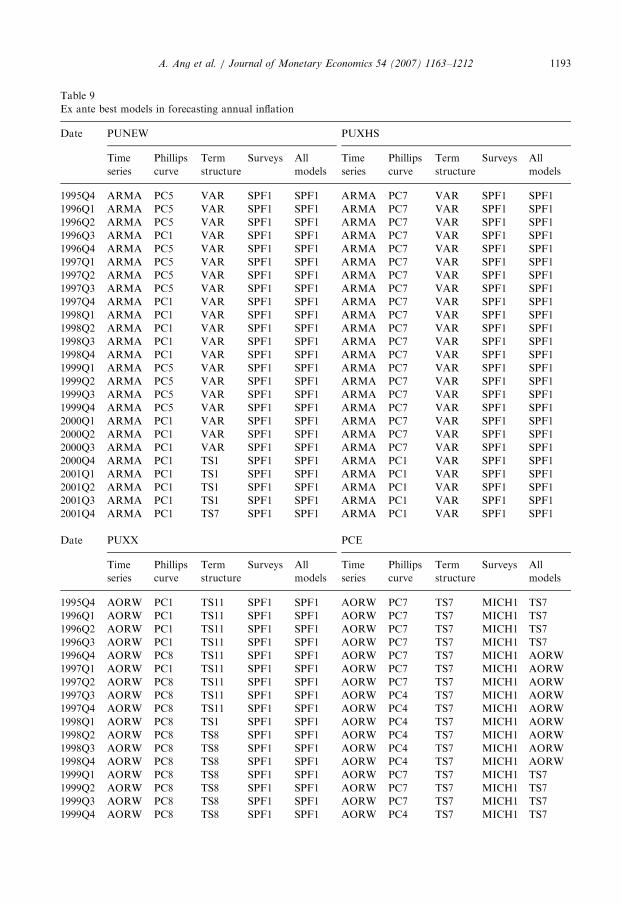
ARTICLE IN PRESS
Table 9
Ex ante best models in forecasting annual inflation
Date PUNEW PUXHS
Time
series
Phillips
curve
Term
structure
Surveys All
models
Time
series
Phillips
curve
Term
structure
Surveys All
models
1995Q4 ARMA PC5 VAR SPF1 SPF1 ARMA PC7 VAR SPF1 SPF1
1996Q1 ARMA PC5 VAR SPF1 SPF1 ARMA PC7 VAR SPF1 SPF1
1996Q2 ARMA PC5 VAR SPF1 SPF1 ARMA PC7 VAR SPF1 SPF1
1996Q3 ARMA PC1 VAR SPF1 SPF1 ARMA PC7 VAR SPF1 SPF1
1996Q4 ARMA PC5 VAR SPF1 SPF1 ARMA PC7 VAR SPF1 SPF1
1997Q1 ARMA PC5 VAR SPF1 SPF1 ARMA PC7 VAR SPF1 SPF1
1997Q2 ARMA PC5 VAR SPF1 SPF1 ARMA PC7 VAR SPF1 SPF1
1997Q3 ARMA PC5 VAR SPF1 SPF1 ARMA PC7 VAR SPF1 SPF1
1997Q4 ARMA PC1 VAR SPF1 SPF1 ARMA PC7 VAR SPF1 SPF1
1998Q1 ARMA PC1 VAR SPF1 SPF1 ARMA PC7 VAR SPF1 SPF1
1998Q2 ARMA PC1 VAR SPF1 SPF1 ARMA PC7 VAR SPF1 SPF1
1998Q3 ARMA PC1 VAR SPF1 SPF1 ARMA PC7 VAR SPF1 SPF1
1998Q4 ARMA PC1 VAR SPF1 SPF1 ARMA PC7 VAR SPF1 SPF1
1999Q1 ARMA PC5 VAR SPF1 SPF1 ARMA PC7 VAR SPF1 SPF1
1999Q2 ARMA PC5 VAR SPF1 SPF1 ARMA PC7 VAR SPF1 SPF1
1999Q3 ARMA PC5 VAR SPF1 SPF1 ARMA PC7 VAR SPF1 SPF1
1999Q4 ARMA PC5 VAR SPF1 SPF1 ARMA PC7 VAR SPF1 SPF1
2000Q1 ARMA PC1 VAR SPF1 SPF1 ARMA PC7 VAR SPF1 SPF1
2000Q2 ARMA PC1 VAR SPF1 SPF1 ARMA PC7 VAR SPF1 SPF1
2000Q3 ARMA PC1 VAR SPF1 SPF1 ARMA PC7 VAR SPF1 SPF1
2000Q4 ARMA PC1 TS1 SPF1 SPF1 ARMA PC1 VAR SPF1 SPF1
2001Q1 ARMA PC1 TS1 SPF1 SPF1 ARMA PC1 VAR SPF1 SPF1
2001Q2 ARMA PC1 TS1 SPF1 SPF1 ARMA PC1 VAR SPF1 SPF1
2001Q3 ARMA PC1 TS1 SPF1 SPF1 ARMA PC1 VAR SPF1 SPF1
2001Q4 ARMA PC1 TS7 SPF1 SPF1 ARMA PC1 VAR SPF1 SPF1
Date PUXX PCE
Time
series
Phillips
curve
Term
structure
Surveys All
models
Time
series
Phillips
curve
Term
structure
Surveys All
models
1995Q4 AORW PC1 TS11 SPF1 SPF1 AORW PC7 TS7 MICH1 TS7
1996Q1 AORW PC1 TS11 SPF1 SPF1 AORW PC7 TS7 MICH1 TS7
1996Q2 AORW PC1 TS11 SPF1 SPF1 AORW PC7 TS7 MICH1 TS7
1996Q3 AORW PC1 TS11 SPF1 SPF1 AORW PC7 TS7 MICH1 TS7
1996Q4 AORW PC8 TS11 SPF1 SPF1 AORW PC7 TS7 MICH1 AORW
1997Q1 AORW PC1 TS11 SPF1 SPF1 AORW PC7 TS7 MICH1 AORW
1997Q2 AORW PC8 TS11 SPF1 SPF1 AORW PC7 TS7 MICH1 AORW
1997Q3 AORW PC8 TS11 SPF1 SPF1 AORW PC4 TS7 MICH1 AORW
1997Q4 AORW PC8 TS11 SPF1 SPF1 AORW PC4 TS7 MICH1 AORW
1998Q1 AORW PC8 TS1 SPF1 SPF1 AORW PC4 TS7 MICH1 AORW
1998Q2 AORW PC8 TS8 SPF1 SPF1 AORW PC4 TS7 MICH1 AORW
1998Q3 AORW PC8 TS8 SPF1 SPF1 AORW PC4 TS7 MICH1 AORW
1998Q4 AORW PC8 TS8 SPF1 SPF1 AORW PC4 TS7 MICH1 AORW
1999Q1 AORW PC8 TS8 SPF1 SPF1 AORW PC7 TS7 MICH1 TS7
1999Q2 AORW PC8 TS8 SPF1 SPF1 AORW PC7 TS7 MICH1 TS7
1999Q3 AORW PC8 TS8 SPF1 SPF1 AORW PC7 TS7 MICH1 TS7
1999Q4 AORW PC8 TS8 SPF1 SPF1 AORW PC4 TS7 MICH1 TS7
A. Ang et al. / Journal of Monetary Economics 54 (2007) 1163–1212 1193
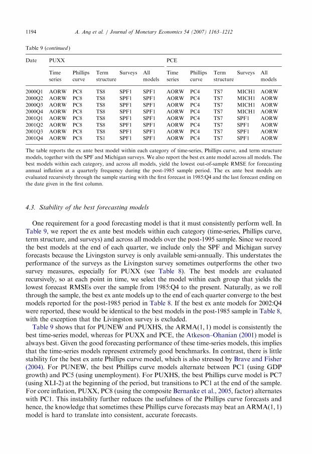
ARTICLE IN PRESS
Table 9 (continued )
Date PUXX PCE
Time
series
Phillips
curve
Term
structure
Surveys All
models
Time
series
Phillips
curve
Term
structure
Surveys All
models
2000Q1 AORW PC8 TS8 SPF1 SPF1 AORW PC4 TS7 MICH1 AORW
2000Q2 AORW PC8 TS8 SPF1 SPF1 AORW PC4 TS7 MICH1 AORW
2000Q3 AORW PC8 TS8 SPF1 SPF1 AORW PC4 TS7 MICH1 AORW
2000Q4 AORW PC8 TS8 SPF1 SPF1 AORW PC4 TS7 MICH1 AORW
2001Q1 AORW PC8 TS8 SPF1 SPF1 AORW PC4 TS7 SPF1 AORW
2001Q2 AORW PC8 TS8 SPF1 SPF1 AORW PC4 TS7 SPF1 AORW
2001Q3 AORW PC8 TS8 SPF1 SPF1 AORW PC4 TS7 SPF1 AORW
2001Q4 AORW PC8 TS1 SPF1 SPF1 AORW PC4 TS7 SPF1 AORW
The table reports the ex ante best model within each category of time-series, Phillips curve, and term structure
models, together with the SPF and Michigan surveys. We also report the best ex ante model across all models. The
best models within each category, and across all models, yield the lowest out-of-sample RMSE for forecasting
annual inflation at a quarterly frequency during the post-1985 sample period. The ex ante best models are
evaluated recursively through the sample starting with the first forecast in 1985:Q4 and the last forecast ending on
the date given in the first column.
A. Ang et al. / Journal of Monetary Economics 54 (2007) 1163–12121194
4.3. Stability of the best forecasting models
One requirement for a good forecasting model is that it must consistently perform well. InTable 9, we report the ex ante best models within each category (time-series, Phillips curve,term structure, and surveys) and across all models over the post-1995 sample. Since we recordthe best models at the end of each quarter, we include only the SPF and Michigan surveyforecasts because the Livingston survey is only available semi-annually. This understates theperformance of the surveys as the Livingston survey sometimes outperforms the other twosurvey measures, especially for PUXX (see Table 8). The best models are evaluatedrecursively, so at each point in time, we select the model within each group that yields thelowest forecast RMSEs over the sample from 1985:Q4 to the present. Naturally, as we rollthrough the sample, the best ex ante models up to the end of each quarter converge to the bestmodels reported for the post-1985 period in Table 8. If the best ex ante models for 2002:Q4were reported, these would be identical to the best models in the post-1985 sample in Table 8,with the exception that the Livingston survey is excluded.Table 9 shows that for PUNEW and PUXHS, the ARMAð1; 1Þ model is consistently the
best time-series model, whereas for PUXX and PCE, the Atkeson–Ohanian (2001) model isalways best. Given the good forecasting performance of these time-series models, this impliesthat the time-series models represent extremely good benchmarks. In contrast, there is littlestability for the best ex ante Phillips curve model, which is also stressed by Brave and Fisher(2004). For PUNEW, the best Phillips curve models alternate between PC1 (using GDPgrowth) and PC5 (using unemployment). For PUXHS, the best Phillips curve model is PC7(using XLI-2) at the beginning of the period, but transitions to PC1 at the end of the sample.For core inflation, PUXX, PC8 (using the composite Bernanke et al., 2005, factor) alternateswith PC1. This instability further reduces the usefulness of the Phillips curve forecasts andhence, the knowledge that sometimes these Phillips curve forecasts may beat an ARMAð1; 1Þmodel is hard to translate into consistent, accurate forecasts.
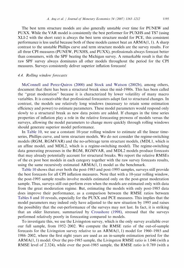
ARTICLE IN PRESSA. Ang et al. / Journal of Monetary Economics 54 (2007) 1163–1212 1195
The best term structure models are also generally unstable over time for PUNEW andPUXX. While the VAR model is consistently the best performer for PUXHS and TS7 (usingXLI-2 with the short rate) is always the best term structure model for PCE, this consistentperformance is less useful because both of these models cannot beat an ARMAð1; 1Þ. A sharpcontrast to the unstable Phillips curve and term structure models are the survey results. Forall three CPI measures (PUNEW, PUXHS, and PUXX), professionals always forecast betterthan consumers, with the SPF beating the Michigan survey. A remarkable result is that theraw SPF survey always dominates all other models throughout the period for the CPImeasures. Surveys consistently deliver superior inflation forecasts!
4.4. Rolling window forecasts
McConnell and Perez-Quiros (2000) and Stock and Watson (2002b), among others,document that there has been a structural break since the mid-1980s. This has been calledthe ‘‘great moderation’’ because it is characterized by lower volatility of many macrovariables. It is conceivable that professional forecasters adapt fast to structural changes. Incontrast, the models use relatively long windows (necessary to retain some estimationefficiency and power) to estimate parameters. These model parameters would respond onlyslowly to a structural break as new data points are added. If changes in the time seriesproperties of inflation play a role in the relative forecasting prowess of models versus thesurveys, allowing the model parameters to change more quickly through rolling windowsshould generate superior model performance.
In Table 10, we use a constant 10-year rolling window to estimate all the linear time-series, Phillips curve, and term structure models. We do not consider the regime-switchingmodels (RGM, RGMVAR) and the no-arbitrage term structure models, (MDL1, which isan affine model, and MDL2, which is a regime-switching model). The regime-switchingdata generating processes in the RGM, RGMVAR, and MDL2 models produce forecaststhat may already potentially account for structural breaks. We report the relative RMSEsof the ex post best models in each category together with the raw survey forecasts results,using the same recursively estimated ARMAð1; 1Þ model as the benchmark.
Table 10 shows that over both the post-1985 and post-1995 samples, surveys still providethe best forecasts for all CPI inflation measures. Note that with a 10-year rolling window,the post-1995 sample results involve models estimated only on the post-great moderationsample. Thus, surveys still out-perform even when the models are estimated only with datafrom the great moderation regime. But, estimating the models with only post-1985 datadoes improve their performance, as a comparison between the RMSE ratios betweenTables 8 and 10 reveals, especially for the PUXX and PCE measures. This implies that themodel parameters may indeed only have adjusted to the new situation by 1995 and raisesthe possibility that the out-performance of the surveys may not last. In fact, it is strikingthat an older literature, summarized by Croushore (1998), stressed that the surveysperformed relatively poorly in forecasting compared to models.
To investigate this, we use the Livingston survey, which is the only survey available overour full sample, from 1952–2002. We compute the RMSE ratio of the out-of-sampleforecasts for the Livingston survey relative to an ARMAð1; 1Þ model for 1960–1985 and1986–2002, where the first eight years are used as an in-sample estimation period for theARMAð1; 1Þ model. Over the pre-1985 sample, the Livingston RMSE ratio is 1.046 (with aRMSE level of 2.324), while over the post-1985 sample, the RMSE ratio is 0.789 (with a
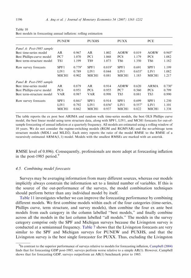
ARTICLE IN PRESS
Table 10
Best models in forecasting annual inflation: rolling estimation
PUNEW PUXHS PUXX PCE
Panel A: Post-1985 sample
Best time-series model AR 0.967 AR 1.002 AORW 0.819 AORW 0:945�
Best Phillips-curve model PC7 1.070 PC1 1.068 PC8 1.179 PC8 1.082
Best term-structure model TS1 1.199 TS9 1.073 TS6 1.350 TS6 1.182
Raw survey forecasts SPF1 0:779� SPF1 0:819� SPF1 0.691 SPF1 1.199
LIV1 0.789 LIV1 0.844 LIV1 0:655� LIV1 1.082
MICH1 0.902 MICH1 0.881 MICH1 1.185 MICH1 1.217
Panel B: Post-1995 sample
Best time-series model AR 0.879 AR 0.914 ADRW 0.620 ARMA 0:730�
Best Phillips-curve model PC6 0.951 PC6 0.955 PC7 0.560 PC6 0.799
Best term-structure model VAR 0.987 VAR 0.998 TS5 0.881 TS3 0.990
Raw survey forecasts SPF1 0:861� SPF1 0.914 SPF1 0.699 SPF1 1.250
LIV1 0.792 LIV1 0:856� LIV1 0:557� LIV1 1.101
MICH1 0.862 MICH1 0.937 MICH1 0.822 MICH1 1.338
The table reports the ex post best ARIMA and random walk time-series models, the best OLS Phillips curve
model, the best linear model using term structure data, along with SPF1, LIV1, and MCH1 forecasts for out-of-
sample forecasting of annual inflation at a quarterly frequency. All models are estimated using a rolling window of
10 years. We do not consider the regime-switching models (RGM and RGMVAR) and the no-arbitrage term
structure models (MDL1 and MLD2). Each entry reports the ratio of the model RMSE to the RMSE of a
recursively estimated ARMAð1; 1Þ model. Models with the smallest RMSEs are marked with an asterisk.
A. Ang et al. / Journal of Monetary Economics 54 (2007) 1163–12121196
RMSE level of 0.896). Consequently, professionals are more adept at forecasting inflationin the post-1985 period.9
4.5. Combining model forecasts
Surveys may be averaging information from many different sources, whereas our modelsimplicitly always constrain the information set to a limited number of variables. If this isthe source of the out-performance of the surveys, the model combination techniquesshould perform better than any individual model by itself.Table 11 investigates whether we can improve the forecasting performance by combining
different models. We first combine models within each of the four categories (time-series,Phillips curve, term structure, and survey models), then combine the four ex ante bestmodels from each category in the column labelled ‘‘best models,’’ and finally combineacross all the models in the last column labelled ‘‘all models.’’ The models in the surveycategory comprise only the SPF and Michigan surveys because the Livingston survey isconducted at a semiannual frequency. Table 7 shows that the Livingston forecasts are verysimilar to the SPF and Michigan surveys for PUNEW and PUXHS, and that theLivingston survey is the best single forecaster for PUXX. Thus, excluding the Livingston
9In contrast to the superior performance of surveys relative to models for forecasting inflation, Campbell (2004)
finds that for forecasting GDP post-1985, surveys perform worse relative to a simple AR(1). However, Campbell
shows that for forecasting GDP, surveys outperform an AR(1) benchmark prior to 1985.
ARTICLE IN PRESS
Table 11
Combined forecasts of annual inflation
Model combination
method
Time-
series
Phillips
curve
Term
structure
Surveys Best
models
All models
PUNEW Mean 0.898 1.123 1.057 0.851 0.992 0.998
Median 0.934 1.093 1.079 0.851 1.016 1.045
OLS 0.970 1.007 1.116 0.858 0.867 0.876
Equal weight prior 0.955 1.007 1.102 0.858 0.861 0.879
Unit weight prior 0.977 0.951 1.115 0.859 0.862 0.873
Best individual
model
1.000 0.960 1.207 0.861 0.861 0.861
PUXHS Mean 0.954 1.065 1.012 0.921 0.975 0.992
Median 0.953 1.082 1.053 0.921 1.009 1.039
OLS 0.963 1.001 1.069 0.917 0.919 0.924
Equal weight prior 0.950 1.008 1.058 0.918 0.920 0.935
Unit weight prior 0.977 0.992 1.085 0.916 0.914 0.914
Best individual
model
1.000 1.029 1.137 0.914 0.914 0.914
PUXX Mean 0.835 1.547 1.322 0.719 0.727 1.235
Median 0.940 1.167 1.211 0.719 0.735 1.052
OLS 0.631 0.885 0.964 0.699 0.665 0.706
Equal weight prior 0.687 0.878 0.956 0.699 0.652 0.661
Unit weight prior 0.650 0.836 0.947 0.699 0.658 0.658
Best individual
model
0.620 0.779 0.977 0.699 0.699 0.699
PCE Mean 0.968 1.160 1.127 1.285 0.999 1.105
Median 0.979 1.136 1.130 1.285 0.999 1.118
OLS 0.935 0.974 1.019 1.288 0.921 0.964
Equal weight prior 0.938 0.984 1.017 1.287 0.922 0.968
Unit weight prior 0.917 0.967 1.010 1.287 0.911 0.948
Best individual
model
0.921 1.057 1.106 1.289 0.887 0.887
The table reports the RMSEs relative to the ARMAð1; 1Þ model for forecasting annual inflation at a quarterly
frequency out-of-sample from 1995:Q4 to 2002:Q4 by combining models within each category (time-series,
Phillips curve, term structure, surveys), using the ex ante best models in each category, or over all models.
Forecasts reported include the mean and median forecasts, and linear combinations of forecasts using recursively
computed weights computed from OLS, or model combination regressions with various priors. We investigate an
equal weight prior and a prior that places only a unit weight on the best ex ante model. We consider only
unadjusted SPF and Michigan survey forecasts in the survey category. For comparison, the last row in each panel
reports the relative RMSE of using the ex ante best performing single forecast model at each period (as reported in
Table 9).
A. Ang et al. / Journal of Monetary Economics 54 (2007) 1163–1212 1197
survey places a conservative higher bound on the RMSEs for the forecast combinationsinvolving surveys.
We use five methods of model combination: means or medians over all the models,linear combinations using weights recursively computed by OLS, and linear combina-tions using weights recursively computed by mixed combination regressions either withan equal-weight prior or a prior that places a unit weight on the ex ante best model.We start the model combination regressions in 1995:Q4 using realized inflation and the
ARTICLE IN PRESSA. Ang et al. / Journal of Monetary Economics 54 (2007) 1163–12121198
out-of-sample forecasts over 1985:Q4 to 1995:Q4. At each subsequent period, we advancethe data sample by one quarter and re-run the model combination regression to obtain theslope coefficient estimates. For comparison, the last row in each panel reports the RMSEratio, relative to an ARMAð1; 1Þ forecast, of the recursively updated ex ante bestperforming individual model, as reported in Table 9.10
There are three main findings in Table 11. First, using mean or median forecasts mostlydoes not improve the forecast performance relative to the best individual ex ante model.There are 24 cases to consider: four inflation measures and six different sets of modelcombinations. Combining forecasts by taking their means only improves out-of-sampleforecasts in six out of 24 cases. Taking medians produces the same results, improvingforecasts for exactly the same cases as taking means. The mean or median combinationmethods work best for PUNEW and PUXHS using time-series models. However, whenthese forecasting improvements occur for model combinations, the improvements aresmall. Thus, simple methods of combining forecasts provide little additional predictivepower relative to the best model.Second, updating the model weights based on previous model performance does not
always lead to superior performance. For the Phillips Curve models, OLS modelcombinations outperform means and medians for all inflation measures. However, whenOLS model combinations are taken across all models, using an OLS combination is neverbetter than the best individual model.Finally, the performance of the equal-weight prior and the unit prior that places weight
on only the best ex ante model are generally close to the OLS forecast combinationmethod. Across all models, the unit weight prior produces lower RMSE ratios than theOLS or equal-weight priors. However, it is only for PUXX that the various regression-based model combination methods produce better forecasts than the best individualforecasts. For PUNEW, PUXHS, and PCE, the best individual models beat the modelcombinations, and for PUNEW and PUXHS, the best individual ex ante forecasts aresurveys.To help interpret the results, we investigate the ex ante OLS weights on some selected
models. In Fig. 2, we plot the OLS slope estimates of regression (18) for various inflationmeasures over the period of 1995:Q4–2002:Q4. For clarity, we restrict the regression tocombinations of the ex ante best model within each category (time-series, Phillips Curve,term structure) together with the SPF survey. Note that by choosing the best model in eachcategory, we handicap the survey forecasts. We compute the weights in the regressionrecursively like the forecasts in Table 11; that is, we start in 1995:Q4, and recursivelycompute forecasts from 1985:Q4 to 1995:Q4.Fig. 2 shows that when forecasting all the CPI inflation measures (PUNEW, PUXHS,
and PUXX), the data consistently place the largest ex ante weights on survey forecasts andvery little weight on the other models. The weights on the SPF survey forecast are generallyconstant and lie around 0.8 for PUNEW, PUXX, and PUXHS. There is no consistent bestmodel that dominates for the remaining 0.1–0.2 weights. The weights on the time-series
10We also ask the question whether ex post, a particular combination of models would have performed better
than individual forecasts. This ex post analysis cannot be used for actual forecasting, but indicates which models
would have been most successful forecasting inflation out-of-sample ex post. For the ex post combinations, we
find that the improvement generated by the combined forecasts is also relatively minor, even for the unit-weight
prior model, which uses forward-looking information to find the best performing model over the whole sample.
These results are available upon request.
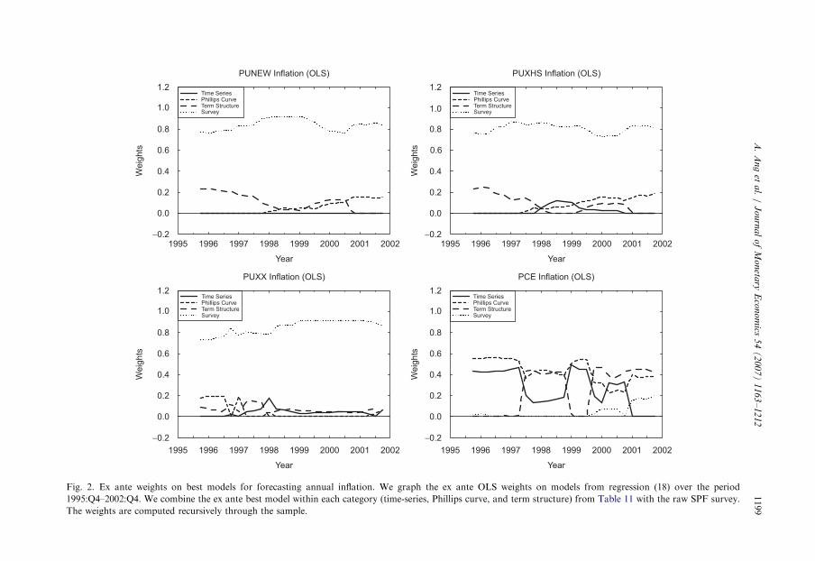
ARTIC
LEIN
PRES
S
1.2
1.0
0.8
0.6
0.4
0.2
0.0
−0.21995 1996 1997 1998 1999 2000 2001 2002
Year
1995 1996 1997 1998 1999 2000 2001 2002
Year
1995 1996 1997 1998 1999 2000 2001 2002
Year
1995 1996 1997 1998 1999 2000 2001 2002
Year
We
igh
ts
1.2
1.0
0.8
0.6
0.4
0.2
0.0
−0.2
We
igh
ts
1.2
1.0
0.8
0.6
0.4
0.2
0.0
−0.2
We
igh
ts
1.2
1.0
0.8
0.6
0.4
0.2
0.0
−0.2
We
igh
ts
PUNEW Inflation (OLS) PUXHS Inflation (OLS)
PCE Inflation (OLS)PUXX Inflation (OLS)
Fig. 2. Ex ante weights on best models for forecasting annual inflation. We graph the ex ante OLS weights on models from regression (18) over the period
1995:Q4–2002:Q4. We combine the ex ante best model within each category (time-series, Phillips curve, and term structure) from Table 11 with the raw SPF survey.
The weights are computed recursively through the sample.
A.
An
get
al.
/J
ou
rna
lo
fM
on
etary
Eco
no
mics
54
(2
00
7)
11
63
–1
21
21199
ARTICLE IN PRESSA. Ang et al. / Journal of Monetary Economics 54 (2007) 1163–12121200
models are always zero for PUNEW, but temporarily spike upward in the middle of thesample to around 0.15 for PUXHS and 0.20 for PUXX. For PUNEW and PUXHS, thePhillips curves fare best at the beginning of the sample, but the regressions place very littleweight on Phillips curve forecasts at the end of the sample. For PCE inflation, surveyscontain little information. The weight on the best survey stays close to zero until late 1999,then rises to 0.2. For forecasting PCE among the other categories of models, the PhillipsCurve forecast stands out, with weights ranging from 0.2 to 0.6. Term structure modelsreceive the highest weight at the end of the sample. We conclude that combining modelforecasts, at least using the techniques here, is not a very useful forecasting tool, especiallycompared to using just survey data for forecasting CPI inflation.
5. Robustness to non-stationary inflation
5.1. Definition and models
In this section we investigate the robustness of our results to the alternative assumptionthat quarterly inflation is difference stationary. Our exercise is now to forecast four-quarterahead inflation changes:
Etðptþ4;4 � pt;4Þ ¼ Et
X3i¼�3
ð4� jijÞDptþ1þi
" #
¼ Et
X3i¼0
ð4� iÞDptþ1þi
" #þ 4pt � pt;4, ð21Þ
where ptþ4;4 is annual inflation defined in Eq. (2).We now replace quarterly inflation, pt, by quarterly inflation changes, Dptþ1 ¼ ptþ1 � pt
in all the models considered in Sections 3.1–3.3. For example, we estimate an ARMAð1; 1Þon first differences of inflation:
Dptþ1 ¼ mþ fDpt þ c�t þ �tþ1
and an ARðpÞ on first differences of inflation:
Dptþ1 ¼ mþ f1Dpt þ f2Dpt�1 þ � � � þ fpDpt�pþ1 þ �tþ1.
The OLS Phillips Curve and term structure regressions include quarterly inflation changesas one of the regressors, rather than quarterly inflation. From the models estimated on Dpt,we compute forecasts of inflation changes over the next year, Etðptþ4;4 � pt;4Þ.There are three models for which we do not estimate a counterpart using quarterly
inflation differences. We do not consider a random walk model for inflation changes anddo not specify the no-arbitrage term structure models (MLD1 and MLD2) to have non-stationary inflation dynamics, although we still consider the forecasts of annual inflationchanges implied by the original stationary models. In all other cases, we examine theforecasts of both the original stationary models and the new non-stationary models thatuse first differences of inflation.The original models estimated on inflation levels generate RMSEs for forecasting annual
inflation changes that are identical to the RMSEs for forecasting annual inflation levels.Hence, the question is whether models estimated on differences provide superior forecaststo models estimated on levels. By including a new set of models estimated on inflation
ARTICLE IN PRESSA. Ang et al. / Journal of Monetary Economics 54 (2007) 1163–1212 1201
changes, we also enrich the set of forecasts which we can combine. We maintain theARMAð1; 1Þ model estimated on inflation rate levels as a benchmark.
5.2. Performance of individual models
Table 12 reports the RMSE ratios of the best performing models estimated on levels ordifferences within each model category. Time-series models estimated on levels alwaysprovide lower RMSEs than time-series models estimated on differences. For both Phillipscurve and term structure models, using inflation differences or levels produces similarforecasting performance for both the PUNEW and PUXHS measures. For these inflationmeasures, the Phillips curve models are slightly better estimated on levels, but for termstructure models, there is no clear overall winner. However, for the PUXX and PCEmeasures, Phillips curve and term structure regressions using past inflation changes aremore accurate than regressions with past inflation levels.
Our major finding that surveys generally outperform other model forecasts is robust tospecifying the models in inflation differences. For the CPI inflation measures (PUNEW,PUXHS, PUXX) over the post-1985 sample, surveys deliver lower RMSEs than the besttime-series, Phillips curve, and term structure forecasts. First difference models are mosthelpful for lowering RMSEs for core inflation (PUXX) over the post-1995 sample, wherethe best time-series model estimated on differences (ARMA) produces a relative RMSEratio of 0.649. This is still beaten by the raw Livingston survey, with a RMSE ratio of0.557.11
5.3. Performance of combining models
In this section, we run forecast combination regressions to determine the bestcombination of models to forecast inflation changes (similar to Section 3.6 for inflationlevels). The model weights are computed from the regression:
psþ4;4 � ps;4 ¼Xn
i¼1
oisf
is þ �s;sþ4; s ¼ 1; . . . ; t. (22)
We repeat the exercise of Table 11 and compute ex ante recursive weights over1995:Q4–2002:Q4 using the best ex ante forecasting models in each category and across allmodels. In unreported results available upon request, we find that our original results forforecasting inflation levels also extend to forecasting inflation changes. Specifically, there isgenerally no improvement in combining model forecasts, or when model combinationsresult in out-performance, the improvement is small. Specifically, for PUNEW andPUXHS, using means, medians, OLS, or an equal-weight prior produces higher RMSEsthan the best individual model. For these inflation measures, all model combinations
11We also ran model comparison regressions as in Eq. (17), but with inflation changes on the left-hand side, and
keeping the stationary ARMAð1; 1Þ model as the benchmark model. These results are available upon request. We
find that while generally the models specified in differences do not fare any better than the models specified in
levels in terms of beating the RMSE of a stationary ARMAð1; 1Þ, there are more I(1) models with significant
ð1� lÞ coefficients using Hansen–Hodrick (1980) standard errors. The largest increase occurs for PUXX inflation.
Like the model comparisons for forecasting inflation levels, surveys consistently provide significant improvement
in forecasting CPI inflation changes above an ARMAð1; 1Þ model on levels, especially for the post-1985 sample
period.
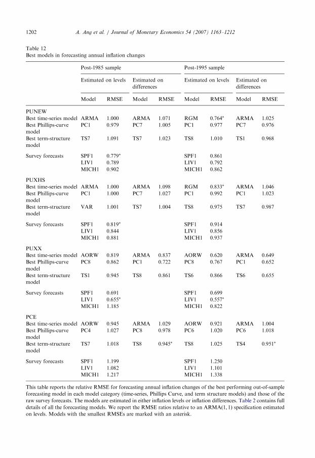
ARTICLE IN PRESS
Table 12
Best models in forecasting annual inflation changes
Post-1985 sample Post-1995 sample
Estimated on levels Estimated on
differences
Estimated on levels Estimated on
differences
Model RMSE Model RMSE Model RMSE Model RMSE
PUNEW
Best time-series model ARMA 1.000 ARMA 1.071 RGM 0:764� ARMA 1.025
Best Phillips-curve
model
PC1 0.979 PC7 1.005 PC1 0.977 PC7 0.976
Best term-structure
model
TS7 1.091 TS7 1.023 TS8 1.010 TS1 0.968
Survey forecasts SPF1 0:779� SPF1 0.861
LIV1 0.789 LIV1 0.792
MICH1 0.902 MICH1 0.862
PUXHS
Best time-series model ARMA 1.000 ARMA 1.098 RGM 0:833� ARMA 1.046
Best Phillips-curve
model
PC1 1.000 PC7 1.027 PC1 0.992 PC1 1.023
Best term-structure
model
VAR 1.001 TS7 1.004 TS8 0.975 TS7 0.987
Survey forecasts SPF1 0:819� SPF1 0.914
LIV1 0.844 LIV1 0.856
MICH1 0.881 MICH1 0.937
PUXX
Best time-series model AORW 0.819 ARMA 0.837 AORW 0.620 ARMA 0.649
Best Phillips-curve
model
PC8 0.862 PC1 0.722 PC8 0.767 PC1 0.652
Best term-structure
model
TS1 0.945 TS8 0.861 TS6 0.866 TS6 0.655
Survey forecasts SPF1 0.691 SPF1 0.699
LIV1 0:655� LIV1 0:557�
MICH1 1.185 MICH1 0.822
PCE
Best time-series model AORW 0.945 ARMA 1.029 AORW 0.921 ARMA 1.004
Best Phillips-curve
model
PC4 1.027 PC8 0.978 PC6 1.020 PC6 1.018
Best term-structure
model
TS7 1.018 TS8 0:945� TS8 1.025 TS4 0:951�
Survey forecasts SPF1 1.199 SPF1 1.250
LIV1 1.082 LIV1 1.101
MICH1 1.217 MICH1 1.338
This table reports the relative RMSE for forecasting annual inflation changes of the best performing out-of-sample
forecasting model in each model category (time-series, Phillips Curve, and term structure models) and those of the
raw survey forecasts. The models are estimated in either inflation levels or inflation differences. Table 2 contains full
details of all the forecasting models. We report the RMSE ratios relative to an ARMAð1; 1Þ specification estimated
on levels. Models with the smallest RMSEs are marked with an asterisk.
A. Ang et al. / Journal of Monetary Economics 54 (2007) 1163–12121202
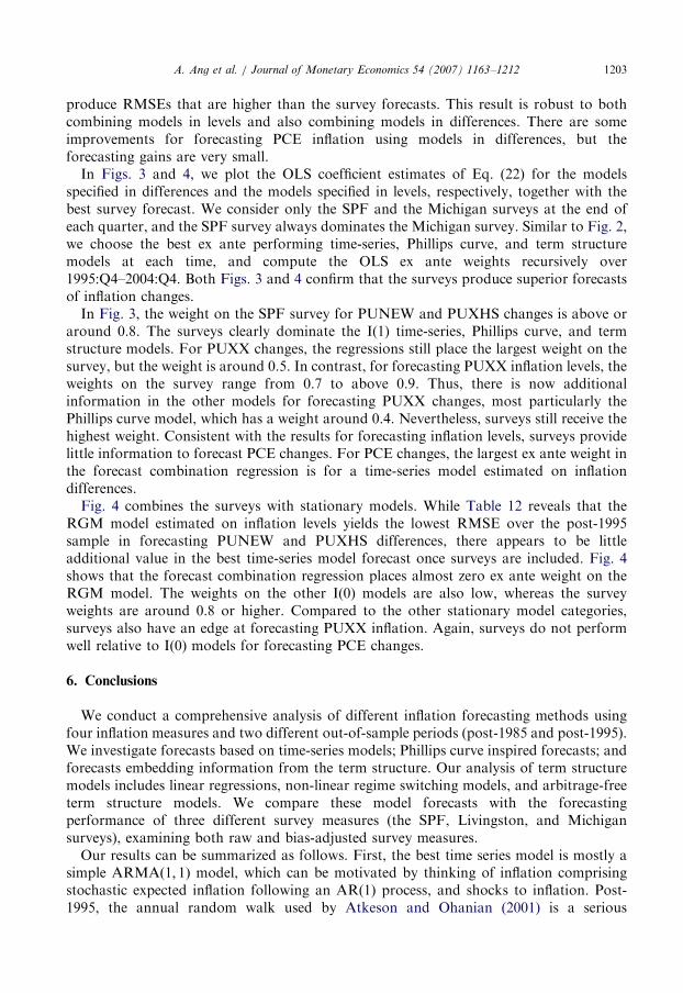
ARTICLE IN PRESSA. Ang et al. / Journal of Monetary Economics 54 (2007) 1163–1212 1203
produce RMSEs that are higher than the survey forecasts. This result is robust to bothcombining models in levels and also combining models in differences. There are someimprovements for forecasting PCE inflation using models in differences, but theforecasting gains are very small.
In Figs. 3 and 4, we plot the OLS coefficient estimates of Eq. (22) for the modelsspecified in differences and the models specified in levels, respectively, together with thebest survey forecast. We consider only the SPF and the Michigan surveys at the end ofeach quarter, and the SPF survey always dominates the Michigan survey. Similar to Fig. 2,we choose the best ex ante performing time-series, Phillips curve, and term structuremodels at each time, and compute the OLS ex ante weights recursively over1995:Q4–2004:Q4. Both Figs. 3 and 4 confirm that the surveys produce superior forecastsof inflation changes.
In Fig. 3, the weight on the SPF survey for PUNEW and PUXHS changes is above oraround 0.8. The surveys clearly dominate the I(1) time-series, Phillips curve, and termstructure models. For PUXX changes, the regressions still place the largest weight on thesurvey, but the weight is around 0.5. In contrast, for forecasting PUXX inflation levels, theweights on the survey range from 0.7 to above 0.9. Thus, there is now additionalinformation in the other models for forecasting PUXX changes, most particularly thePhillips curve model, which has a weight around 0.4. Nevertheless, surveys still receive thehighest weight. Consistent with the results for forecasting inflation levels, surveys providelittle information to forecast PCE changes. For PCE changes, the largest ex ante weight inthe forecast combination regression is for a time-series model estimated on inflationdifferences.
Fig. 4 combines the surveys with stationary models. While Table 12 reveals that theRGM model estimated on inflation levels yields the lowest RMSE over the post-1995sample in forecasting PUNEW and PUXHS differences, there appears to be littleadditional value in the best time-series model forecast once surveys are included. Fig. 4shows that the forecast combination regression places almost zero ex ante weight on theRGM model. The weights on the other I(0) models are also low, whereas the surveyweights are around 0.8 or higher. Compared to the other stationary model categories,surveys also have an edge at forecasting PUXX inflation. Again, surveys do not performwell relative to I(0) models for forecasting PCE changes.
6. Conclusions
We conduct a comprehensive analysis of different inflation forecasting methods usingfour inflation measures and two different out-of-sample periods (post-1985 and post-1995).We investigate forecasts based on time-series models; Phillips curve inspired forecasts; andforecasts embedding information from the term structure. Our analysis of term structuremodels includes linear regressions, non-linear regime switching models, and arbitrage-freeterm structure models. We compare these model forecasts with the forecastingperformance of three different survey measures (the SPF, Livingston, and Michigansurveys), examining both raw and bias-adjusted survey measures.
Our results can be summarized as follows. First, the best time series model is mostly asimple ARMAð1; 1Þ model, which can be motivated by thinking of inflation comprisingstochastic expected inflation following an AR(1) process, and shocks to inflation. Post-1995, the annual random walk used by Atkeson and Ohanian (2001) is a serious
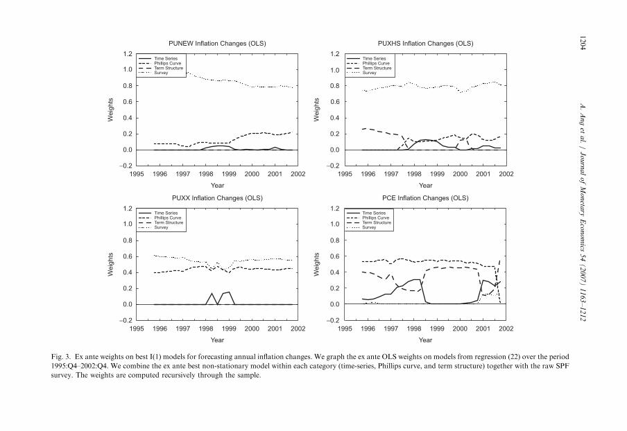
ARTIC
LEIN
PRES
S
1.2
1.0
0.8
0.6
0.4
0.2
0.0
−0.2
1995 1996 1997 1998 1999 2000 2001 2002
Year
1995 1996 1997 1998 1999 2000 2001 2002
Year
1995 1996 1997 1998 1999 2000 2001 2002
Year
1995 1996 1997 1998 1999 2000 2001 2002
Year
We
igh
ts
1.2
1.0
0.8
0.6
0.4
0.2
0.0
−0.2
We
igh
ts
1.2
1.0
0.8
0.6
0.4
0.2
0.0
−0.2W
eig
hts
1.2
1.0
0.8
0.6
0.4
0.2
0.0
−0.2
We
igh
ts
PUNEW Inflation Changes (OLS) PUXHS Inflation Changes (OLS)
PCE Inflation Changes (OLS)PUXX Inflation Changes (OLS)
Fig. 3. Ex ante weights on best I(1) models for forecasting annual inflation changes. We graph the ex ante OLS weights on models from regression (22) over the period
1995:Q4–2002:Q4. We combine the ex ante best non-stationary model within each category (time-series, Phillips curve, and term structure) together with the raw SPF
survey. The weights are computed recursively through the sample.
A.
An
get
al.
/J
ou
rna
lo
fM
on
etary
Eco
no
mics
54
(2
00
7)
11
63
–1
21
21204
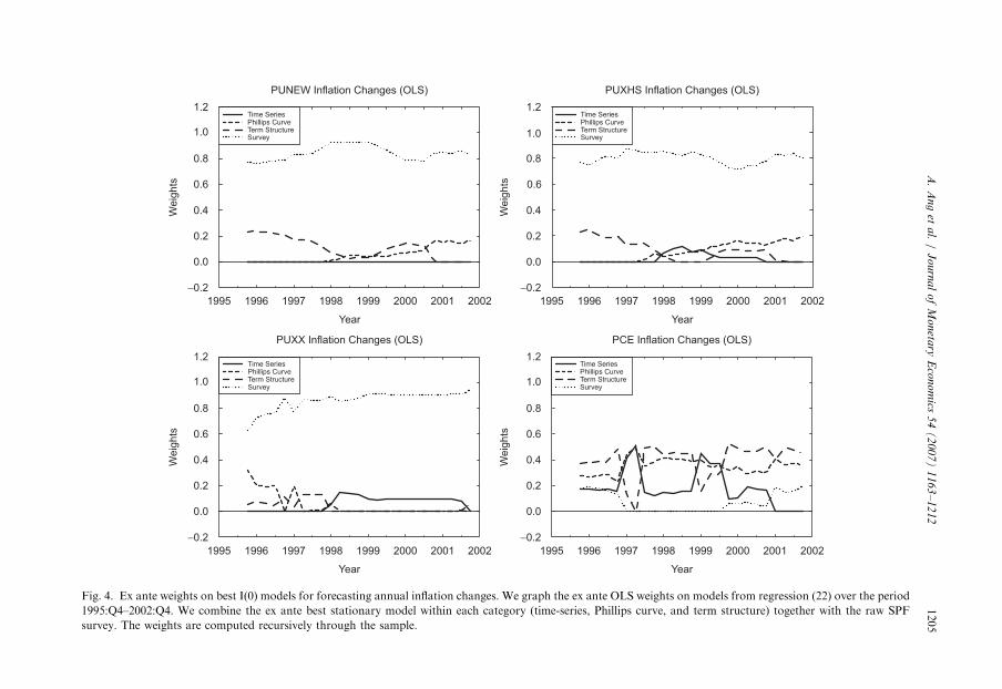
ARTIC
LEIN
PRES
S
1.2
1.0
0.8
0.6
0.4
0.2
0.0
−0.2
1995 1996 1997 1998 1999 2000 2001 2002
Year
1995 1996 1997 1998 1999 2000 2001 2002
Year
1995 1996 1997 1998 1999 2000 2001 2002
Year
1995 1996 1997 1998 1999 2000 2001 2002
Year
We
igh
ts
1.2
1.0
0.8
0.6
0.4
0.2
0.0
−0.2
We
igh
ts
1.2
1.0
0.8
0.6
0.4
0.2
0.0
−0.2
We
igh
ts
1.2
1.0
0.8
0.6
0.4
0.2
0.0
−0.2
We
igh
ts
PUNEW Inflation Changes (OLS) PUXHS Inflation Changes (OLS)
PCE Inflation Changes (OLS)PUXX Inflation Changes (OLS)
Fig. 4. Ex ante weights on best I(0) models for forecasting annual inflation changes. We graph the ex ante OLS weights on models from regression (22) over the period
1995:Q4–2002:Q4. We combine the ex ante best stationary model within each category (time-series, Phillips curve, and term structure) together with the raw SPF
survey. The weights are computed recursively through the sample.
A.
An
get
al.
/J
ou
rna
lo
fM
on
etary
Eco
no
mics
54
(2
00
7)
11
63
–1
21
21205
ARTICLE IN PRESSA. Ang et al. / Journal of Monetary Economics 54 (2007) 1163–12121206
competitor. Second, while the ARMAð1; 1Þ model is hard to beat in terms of RMSEforecast accuracy, it is never the best model. For CPI measures, the survey measuresconsistently deliver better forecasts than ARMAð1; 1Þ models, and in fact, much betterforecasts than Phillips curve-based regressions, term structure models based on OLSregressions, non-linear models, iterated VAR forecasts, and even no-arbitrage termstructure models that use information from the entire cross-section of yields. Naturally,surveys do a relatively poor job at forecasting PCE inflation, which they are not designedto forecast.Some of our results shed light on the validity of some simple explanations of the superior
performance of survey forecasts. One possibility is that the surveys simply aggregateinformation from many different sources, not captured by a single model. The superiorinformation in median survey forecasts may be due to an effect similar to Bayesian modelaveraging, or averaging across potentially hundreds of different individual forecasts andextracting common components (see Stock and Watson, 2002a; Timmermann, 2004). Forexample, it is striking that the Michigan survey, which is conducted among relativelyunsophisticated consumers, beats time-series, Phillips curve, and term structure forecasts.The Livingston and SPF surveys, conducted among professionals, do even better.If there is information in surveys not included in a single model, combining model
forecasts may lead to superior forecasts. However, when we examine forecasts thatcombine information across models or from various data sources (like the Bernanke et al.,2005, index of real activity that uses 65 macro factors measuring real activity), we find thatthe surveys still outperform. Across all models, combination methods of simple means ormedians, or forecast combination regressions which use prior information neveroutperform survey forecasts. In ex ante model combination exercises for forecasting CPIinflation, almost all the weight is placed on survey forecasts. One avenue for futureresearch is to investigate whether alternative techniques for combining forecasts performbetter (see Inoue and Kilian, 2005, for a survey and study of one promising technique).Another potential reason why surveys outperform is because survey information is not
captured in any of the variables or models that we use. If this is the case, our resultsstrongly suggest that it would be informative to include survey forecasts in the largedatasets used to construct a small number of composite factors, which are designed tosummarize aggregate macroeconomic dynamics (see, among others, Bernanke et al., 2005;Stock and Watson, 2005).Our results also have important implications for term structure modelling. Extant
sophisticated no-arbitrage term structure models, while performing well in sample, seemto provide relatively poor forecasts relative to simpler term structure or Phillips curvemodels out-of-sample. A potential solution is to introduce the information present in thesurveys as additional state variables in the term structure models. Pennacchi (1991) wasan early attempt in that direction and Kim and Orphanides (2005) is a recent attemptto build survey expectations into a no-arbitrage quadratic term structure model. Brennanet al. (2004) also recently use the Livingston survey to estimate an affine asset pricingmodel.Finally, surveys may forecast well because they quickly react to changes in the data
generating process for inflation in the post-1985 sample. In particular, since the mid-1980s,the volatility of many macroeconomic series, including inflation, has declined. This ‘‘greatmoderation’’ may also explain why a univariate regime-switching model for inflationprovides relatively good forecasts over this sample period. Nevertheless, when we re-do
ARTICLE IN PRESSA. Ang et al. / Journal of Monetary Economics 54 (2007) 1163–1212 1207
our forecasting exercises using a 10-year rolling window, the surveys forecasts remainsuperior.
We conjecture that the surveys likely perform well for all of these reasons: the pooling oflarge amounts of information; the efficient aggregation of that information; and the abilityto quickly adapt to major changes in the economic environment such as the greatmoderation. While our analysis shows that surveys provide superior forecasts of CPIinflation, the PCE deflator is often the Federal Reserve’s preferred inflation indicator forthe conduct of monetary policy. Since existing surveys target only the CPI index,professional surveys designed to forecast the PCE deflator may also deliver superiorforecasts of PCE inflation.
Appendix A. Computation of West (1996) standard errors
By subtracting f ARMAt from both sides of Eq. (17) and letting eARMA
t;tþ4 denote the forecastresiduals of the ARMAð1; 1Þ model and ex
t;tþ4 denote the forecast residuals of candidatemodel x, we can write
eARMAt;tþ4 ¼ ð1� lÞðeARMA
t;tþ4 � ext;tþ4Þ þ �tþ4;4. (A.1)
The estimated slope coefficient l has the asymptotic distribution:ffiffiffiffiPpðl� lÞ!
dNð0;Eðdtþ4d
0tþ4Þ�1Off Eðdtþ4d
0tþ4Þ�1Þ, (A.2)
where P is the length of the out-sample, Off ¼ varðf t;tþ4Þ, f t;tþ4 ¼ eARMAt;tþ4 ðe
ARMAt;tþ4 � ex
t;tþ4Þ
and dt;tþ4 ¼ eARMAt;tþ4 � ex
t;tþ4. West (1996) derives the long-run asymptotic variance Off aftertaking into account parameter uncertainty.
We use the notation based on West (2006). The forecast horizon is four quarters ahead.For each model i there are P out-of-sample forecasts in all, which rely on estimates of aki � 1 unknown parameter vector yi. The first forecast uses data from a sample of length R
to predict a time t ¼ ðRþ 4Þ variable, while the last forecast uses data from time t ¼
Rþ P� 1 � T to forecast a time t ¼ T þ 4 variable. The total sample size isRþ P� 1þ 4 ¼ T þ 4.
For the ith candidate model, yi, the small-sample estimate of the parameters yi satisfies
yiðtÞ � yi ¼ BiðtÞHiðtÞ, (A.3)
where BiðtÞ is a ki � qi matrix and HiðtÞ is a qi � 1 vector. The vector HiðtÞ representsorthogonality conditions of the model and the matrix BiðtÞ is a linear combination of theorthogonality conditions to recover the parameters. We assume that BiðtÞ!
pBi, where Bi is
a matrix with rank ki. The moment conditions HiðtÞ are given by12
HiðtÞ ¼1
t
Xt
s¼1
hisðyiÞ, (A.4)
for the recursive forecast case which we investigate, where hisðyiÞ are qi � 1 orthogonality
conditions. For models estimated by maximum likelihood, the matrix BiðtÞ is the inverse of
12West and McCracken (1998) derive similar forms for Off under the cases of rolling and fixed out-of-sample
forecasts.
ARTICLE IN PRESSA. Ang et al. / Journal of Monetary Economics 54 (2007) 1163–12121208
the Hessian and hitðyiÞ is the score. For linear models in the form of yt ¼ X i0
t yiþ �t, BiðtÞ ¼
EðX itX
i0t Þ�1 and hi
tðyiÞ ¼ X i0t ðyt � X i0
t yiÞ.We stack the parameters of the ARMAð1; 1Þ benchmark model and the parameters of
the ith candidate model in the vector y ¼ ðyARMA; yiÞ. Then, we can write yðtÞ � y ¼BðtÞHðtÞ, where HðtÞ ¼ ð1=tÞ
Pts¼1 hsðyÞ, where
BðtÞ ¼BARMAðtÞ 0
0 BiðtÞ
" #,
htðyÞ ¼hARMA
t ðyARMAÞ
hitðyiÞ
" #, (A.5)
and BðtÞ!p
B, where
B ¼BARMA 0
0 Bi
" #. (A.6)
We define the derivative F of the moment conditions with respect to y as
F ¼ Eqf t;tþ4ðyÞ
qy
� �¼
F1
F2
" #, (A.7)
where F1 and F 2 are given by
F 1 ¼ Eqf t;tþ4ðyÞqyARMA
� �¼ E ð2eARMA
t;tþ4 � ext;tþ4Þ
qeARMAt;tþ4
qyARMA
" #,
F 2 ¼ Eqf t;tþ4ðyÞ
qyi
� �¼ �E eARMA
t;tþ4
qext;tþ4
qyi
� �. (A.8)
Finally, for the asymptotic results, we need P!1 and R!1 with
r ¼ limT!1
P
Ro1. (A.9)
Following West (2006), we define the constants lfh and lhh
lfh ¼ 1� r�1 lnð1þ rÞ,
lhh ¼ 2½1� r�1 lnð1þ rÞ�. (A.10)
Under these assumptions, West (1996) derives that the asymptotic variance Off is givenby
Off ¼ Sff þ lfhðFBS0fh þ SfhB0F 0Þ þ lhhFBVhhB0F 0, (A.11)
where
Sff ¼X1
j¼�1
E½ðf t;tþ4 � Ef t;tþ4Þðf t�j;t�jþ4 � Ef t;tþ4Þ0�,
ARTICLE IN PRESSA. Ang et al. / Journal of Monetary Economics 54 (2007) 1163–1212 1209
Sfh ¼X1
j¼�1
E½ðf t;tþ4 � Ef t;tþ4Þh0t�j�,
Shh ¼X1
j¼�1
E½hth0t�j�. (A.12)
Note that the estimate without parameter uncertainty is simply Sff , and taking intoaccount parameter uncertainty can increase or decrease the long-run variance of ldepending on the covariances of f t;tþ4 with htþ4.
A consistent estimator can be constructed using the sample counterparts. In particular,we compute lfh and lhh setting r ¼ P=R,
F ¼1
P
XT
t¼R
qf ðyÞqy
�����y¼y
,
B � BðTÞ!p
B, (A.13)
and construct f t;tþ4 ¼ f t;tþ4ðyðtÞÞ and ht ¼ htðyðtÞÞ using the estimates yðtÞ, which arerecursively updated each time using data up to time t. The sample covariances, Sff , Sfh andShh converge to their population equivalents in Eq. (A.12). To estimate these, we define thevector of moments
gt ¼ ½f t;tþ4 F Bht�. (A.14)
To construct a non-singular estimate for the covariance of gt, which we denote as O, we usea Newey–West (1987) covariance estimator with three lags. We partition O as the 2� 2matrix
O ¼O11 O12
O21 O22
" #. (A.15)
Then, a consistent estimate of Off is given by
Off ¼ O11 þ lfhðO12 þ O21Þ þ lhhO22. (A.16)
References
Ang, A., Bekaert, G., 2006a. Regime switches in interest rates. Journal of Business and Economic Statistics 20,
163–182.
Ang, A., Piazzesi, M., Wei, M., 2006a. What does the yield curve tell us about GDP growth? Journal of
Econometrics 131, 359–403.
Ang, A., Bekaert, G., Wei, M., 2006b. The term structure of real rates and expected inflation. Working paper,
Columbia University.
Atkeson, A., Ohanian, L.E., 2001. Are Phillips curves useful for forecasting inflation? Federal Reserve Bank of
Minneapolis Quarterly Review 25, 2–11.
Bai, J., Ng, S., 2004. A panic attack on unit roots and cointegration. Econometrica 72, 1127–1177.
Bates, J.M., Granger, C.W.J., 1969. The combination of forecasts. Operations Research Quarterly 20, 451–468.
Bekaert, G., Hodrick, R.J., Marshall, D., 2001. Peso problem explanations for term structure anomalies. Journal
of Monetary Economics 48, 241–270.
ARTICLE IN PRESSA. Ang et al. / Journal of Monetary Economics 54 (2007) 1163–12121210
Bekaert, G., Cho, S., Moreno, A., 2005. New Keynesian macroeconomics and the term structure. Working paper,
Columbia University.
Bernanke, B.S., Boivin, J., 2003. Monetary policy in a data-rich environment. Journal of Monetary Economics 50,
525–546.
Bernanke, B.S., Boivin, J., Eliasz, P., 2005. Measuring the effects of monetary policy: a factor-augmented vector
autoregressive (FAVAR) approach. Quarterly Journal of Economics 120, 387–422.
Boivin, J., Ng, S., 2006. Are more data always better for factor analysis? Journal of Econometrics, forthcoming.
Brave, S., Fisher, J.D.M., 2004. In search of a robust inflation forecast. Federal Reserve Bank of Chicago
Economic Perspectives 28, 12–30.
Brennan, M.J., Wang, A.W., Xia, Y., 2004. Estimation and test of a simple model of intertemporal capital asset
pricing. Journal of Finance 59, 1743–1775.
Bryan, M.F., Cecchetti, S.G., 1993. The consumer price index as a measure of inflation. Economic Review of the
Federal Reserve Bank of Cleveland 29, 15–24.
Campbell, S.D., 2004. Volatility, predictability and uncertainty in the great moderation: evidence from the survey
of professional forecasters. Working paper, Federal Reserve Board of Governors.
Carlson, J.A., 1977. A study of price forecasts. Annals of Economic and Social Measurement 1, 27–56.
Cecchetti, S., Chu, R., Steindel, C., 2000. The unreliability of inflation indicators. Federal Reserve Bank of
New York Current Issues in Economics and Finance 6, 1–6.
Chen, R.R., Scott, L., 1993. Maximum likelihood estimation for a multi-factor equilibrium model of the term
structure of interest rates. Journal of Fixed Income 3, 14–31.
Clark, T.E., 1999. A comparison of the CPI and the PCE price index. Federal Reserve Bank of Kansas City
Economic Review 3, 15–29.
Clark, T.E., McCracken, M.W., 2006. The predictive content of the output gap for inflation: resolving in-sample
and out-of-sample evidence. Journal of Money, Credit and Banking, forthcoming.
Clemen, R.T., 1989. Combining forecasts: a review and annotated bibliography. International Journal of
Forecasting 5, 559–581.
Cochrane, J., Piazzesi, M., 2005. Bond risk premia. American Economic Review 95 (1), 138–160.
Cogley, T., Sargent, T.J., 2005. Drifts and volatilities: monetary policies and outcomes in the post WWII U.S.
Review of Economic Dynamics 8, 262–302.
Croushore, D., 1998. Evaluating inflation forecasts. Working Paper 98-14, Federal Reserve Bank of St. Louis.
Curtin, R.T., 1996. Procedure to estimate price expectations. Mimeo, University of Michigan Survey Research
Center.
Dai, Q., Singleton, K.J., 2002. Expectation puzzles, time-varying risk premia, and affine models of the term
structure. Journal of Financial Economics 63, 415–441.
Diebold, F.X., 1989. Forecast combination and encompassing: reconciling two divergent literatures. International
Journal of Forecasting 5, 589–592.
Diebold, F.X., Lopez, J.A., 1996. Forecasting evaluation and combination. In: Maddala, G.S., Rao, C.R. (Eds.),
Handbook of Statistics. Elsevier, Amsterdam, pp. 241–268.
Duffee, G.R., 2002. Term premia and the interest rate forecasts in affine models. Journal of Finance 57, 405–443.
Duffie, D., Kan, R., 1996. A yield-factor model of interest rates. Mathematical Finance 6, 379–406.
Estrella, A., Mishkin, F.S., 1997. The predictive power of the term structure of interest rates in Europe and the
United States: implications for the European Central Bank. European Economic Review 41, 1375–1401.
Evans, M.D.D., Lewis, K.K., 1995. Do expected shifts in inflation affect estimates of the long-run Fisher relation?
Journal of Finance 50, 225–253.
Evans, M.D.D., Wachtel, P., 1993. Inflation regimes and the sources of inflation uncertainty. Journal of Money,
Credit and Banking 25, 475–511.
Fama, E.F., 1975. Short-term interest rates as predictors of inflation. American Economic Review 65, 269–282.
Fama, E.F., Gibbons, M.R., 1984. A comparison of inflation forecasts. Journal of Monetary Economics 13,
327–348.
Fisher, J.D.M., Liu, C.T., Zhou, R., 2002. When can we forecast inflation? Federal Reserve Bank of Chicago
Economic Perspectives 1, 30–42.
Frankel, J.A., Lown, C.S., 1994. An indicator of future inflation extracted from the steepness of the interest rate
yield curve along its entire length. Quarterly Journal of Economics 59, 517–530.
Fuhrer, J., Moore, G., 1995. Inflation persistence. Quarterly Journal of Economics 110, 127–159.
Gali, J., Gertler, M., 1999. Inflation dynamics: a structural econometrics analysis. Journal of Monetary
Economics 44 (2), 195–222.
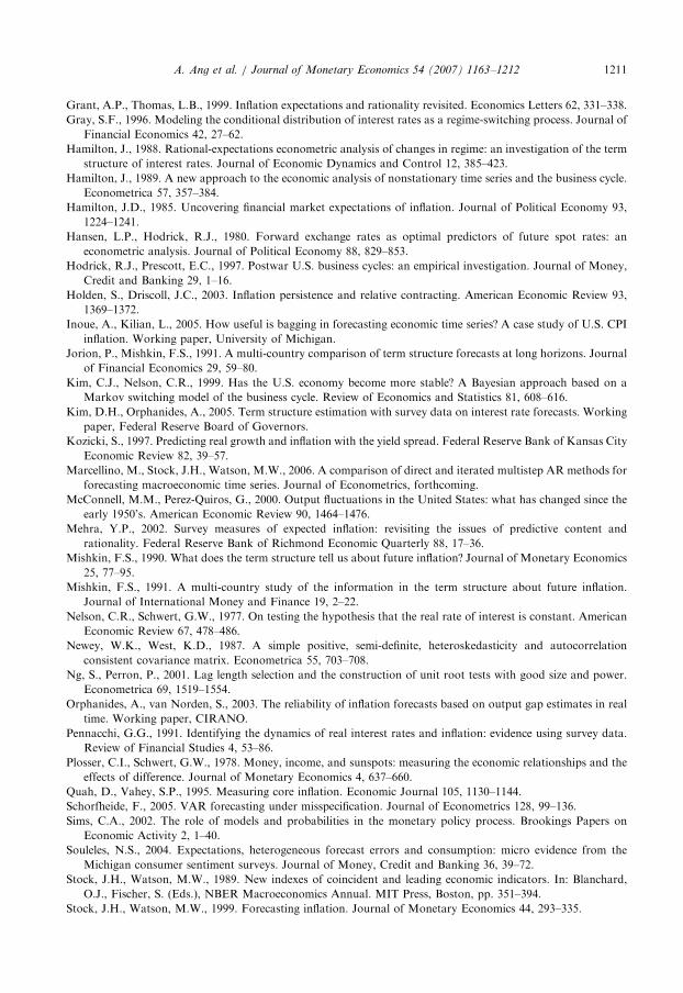
ARTICLE IN PRESSA. Ang et al. / Journal of Monetary Economics 54 (2007) 1163–1212 1211
Grant, A.P., Thomas, L.B., 1999. Inflation expectations and rationality revisited. Economics Letters 62, 331–338.
Gray, S.F., 1996. Modeling the conditional distribution of interest rates as a regime-switching process. Journal of
Financial Economics 42, 27–62.
Hamilton, J., 1988. Rational-expectations econometric analysis of changes in regime: an investigation of the term
structure of interest rates. Journal of Economic Dynamics and Control 12, 385–423.
Hamilton, J., 1989. A new approach to the economic analysis of nonstationary time series and the business cycle.
Econometrica 57, 357–384.
Hamilton, J.D., 1985. Uncovering financial market expectations of inflation. Journal of Political Economy 93,
1224–1241.
Hansen, L.P., Hodrick, R.J., 1980. Forward exchange rates as optimal predictors of future spot rates: an
econometric analysis. Journal of Political Economy 88, 829–853.
Hodrick, R.J., Prescott, E.C., 1997. Postwar U.S. business cycles: an empirical investigation. Journal of Money,
Credit and Banking 29, 1–16.
Holden, S., Driscoll, J.C., 2003. Inflation persistence and relative contracting. American Economic Review 93,
1369–1372.
Inoue, A., Kilian, L., 2005. How useful is bagging in forecasting economic time series? A case study of U.S. CPI
inflation. Working paper, University of Michigan.
Jorion, P., Mishkin, F.S., 1991. A multi-country comparison of term structure forecasts at long horizons. Journal
of Financial Economics 29, 59–80.
Kim, C.J., Nelson, C.R., 1999. Has the U.S. economy become more stable? A Bayesian approach based on a
Markov switching model of the business cycle. Review of Economics and Statistics 81, 608–616.
Kim, D.H., Orphanides, A., 2005. Term structure estimation with survey data on interest rate forecasts. Working
paper, Federal Reserve Board of Governors.
Kozicki, S., 1997. Predicting real growth and inflation with the yield spread. Federal Reserve Bank of Kansas City
Economic Review 82, 39–57.
Marcellino, M., Stock, J.H., Watson, M.W., 2006. A comparison of direct and iterated multistep AR methods for
forecasting macroeconomic time series. Journal of Econometrics, forthcoming.
McConnell, M.M., Perez-Quiros, G., 2000. Output fluctuations in the United States: what has changed since the
early 1950’s. American Economic Review 90, 1464–1476.
Mehra, Y.P., 2002. Survey measures of expected inflation: revisiting the issues of predictive content and
rationality. Federal Reserve Bank of Richmond Economic Quarterly 88, 17–36.
Mishkin, F.S., 1990. What does the term structure tell us about future inflation? Journal of Monetary Economics
25, 77–95.
Mishkin, F.S., 1991. A multi-country study of the information in the term structure about future inflation.
Journal of International Money and Finance 19, 2–22.
Nelson, C.R., Schwert, G.W., 1977. On testing the hypothesis that the real rate of interest is constant. American
Economic Review 67, 478–486.
Newey, W.K., West, K.D., 1987. A simple positive, semi-definite, heteroskedasticity and autocorrelation
consistent covariance matrix. Econometrica 55, 703–708.
Ng, S., Perron, P., 2001. Lag length selection and the construction of unit root tests with good size and power.
Econometrica 69, 1519–1554.
Orphanides, A., van Norden, S., 2003. The reliability of inflation forecasts based on output gap estimates in real
time. Working paper, CIRANO.
Pennacchi, G.G., 1991. Identifying the dynamics of real interest rates and inflation: evidence using survey data.
Review of Financial Studies 4, 53–86.
Plosser, C.I., Schwert, G.W., 1978. Money, income, and sunspots: measuring the economic relationships and the
effects of difference. Journal of Monetary Economics 4, 637–660.
Quah, D., Vahey, S.P., 1995. Measuring core inflation. Economic Journal 105, 1130–1144.
Schorfheide, F., 2005. VAR forecasting under misspecification. Journal of Econometrics 128, 99–136.
Sims, C.A., 2002. The role of models and probabilities in the monetary policy process. Brookings Papers on
Economic Activity 2, 1–40.
Souleles, N.S., 2004. Expectations, heterogeneous forecast errors and consumption: micro evidence from the
Michigan consumer sentiment surveys. Journal of Money, Credit and Banking 36, 39–72.
Stock, J.H., Watson, M.W., 1989. New indexes of coincident and leading economic indicators. In: Blanchard,
O.J., Fischer, S. (Eds.), NBER Macroeconomics Annual. MIT Press, Boston, pp. 351–394.
Stock, J.H., Watson, M.W., 1999. Forecasting inflation. Journal of Monetary Economics 44, 293–335.
ARTICLE IN PRESSA. Ang et al. / Journal of Monetary Economics 54 (2007) 1163–12121212
Stock, J.H., Watson, M.W., 2002a. Forecasting using principal components from a large number of predictors.
Journal of the American Statistical Association 97, 1167–1179.
Stock, J.H., Watson, M.W., 2002b. Has the business cycle changed and why? In: Gertler, M., Rogoff, K. (Eds.),
NBER Macroeconomics Annual 2002. MIT Press, Boston, pp. 159–218.
Stock, J.H., Watson, M.W., 2003. Forecasting output and inflation: the role of asset prices. Journal of Economic
Literature 41, 788–829.
Stock, J.H., Watson, M.W., 2005. An empirical comparison of methods for forecasting using many predictors.
Working paper, Harvard University.
Stockton, D., Glassman, J., 1987. An evaluation of the forecast performance of alternative models of inflation.
Review of Economics and Statistics 69, 108–117.
Theil, H., 1963. On the use of incomplete prior information in regression analysis. Journal of the American
Statistical Association 58, 401–414.
Theil, H., Goldberger, A.S., 1961. On pure and mixed estimation in economics. International Economic Review 2,
65–78.
Thomas, L.B., 1999. Survey measures of expected U.S. inflation. Journal of Economic Perspectives 13, 125–144.
Timmermann, A., 2006. Forecast combinations. In: Elliot, G., Granger, C.W.J., Timmermann, A. (Eds.),
Handbook of Economic Forecasting. Elsevier, Amsterdam in press.
West, K.D., 1996. Asymptotic inference about predictive ability. Econometrica 64, 1067–1084.
West, K.D., 2006. Forecast evaluation. In: Elliott, G., Granger, C.W.J., Timmermann, A. (Eds.), Handbook of
Economic Forecasting. Elsevier, Amsterdam in press.
West, K.D., McCracken, M.W., 1998. Regression-based tests of predictive ability. International Economic
Review 39, 817–840.
Wright, J.H., 2004. Forecasting U.S. inflation by Bayesian model averaging. Working paper, Federal Reserve
Board of Governors.