Do Large Firms with More Technologies Pay More?

Li Yu

a China Center for Human Capital and Labor Market Research

Central University of Finance & Economics, Beijing, China

and

Yongjie Ji

Economics Department, Iowa State University, Ames, IA.

Selected Paper prepared for presentation at the Agricultural & Applied Economics Association 2010 AAEA,CAES, & WAEA Joint Annual Meeting, Denver, Colorado, July 25-27, 2010 Copyright 2010 by Li Yu and Yongjie Ji. All rights reserved. Readers may make verbatim copies of this document for non-commercial purposes by any means, provided that this copyright notice appears on all such copies. 

Do Large Firms with More Technologies Pay More?

Li Yua and Yongjie Jib

May, 2010

Abstract

Investigation of size wage premium in earning’s literature neglects the important role played by technology adoption. This study models the size selection corrected earning’s function by introducing an extra dimension of selection of technology complexity, using a sample from workers in US hog farms. The estimated wage gap between large and small farms is reduced once correction in selection is controlled. Workers compensate monetary income for better work environment, better health and more job security, in which large farms and technologically advanced farms have advantages.

Key Words: size; technology adoption; wage; double selection, agriculture and health

aCentral University of Finance & Economics, Beijing, China; bIowa State University, Ames, IA. Funding support from the U.S. Department of Agriculture and the National Pork Board/Primedia Business is gratefully acknowledged.

  1

I. Introduction

It is commonly observed that larger firms pay higher wages than smaller firms.

This size-wage premium was first documented by Henry Moore (1911), and

corroborated by others, among them, Brown and Medoff (1989) and Oi and

Idson(1999). At the same time, Abowd, Kramarz and Margolis (1999) found that

individual heterogeneity explains a large proportion of the wage variation between

different firm size categories. There is a mixed result on the positive size-wage

premium after endogenous employee selection on firm size is controlled (for example,

Idson and Feaster, 1990; Main and Reilly, 1993). Economists try to unveil the puzzle,

but usually they ignore another important aspect associated with firm size and wages:

larger firms are more likely to adopt more technologies and there are

complementarities between technology adoption and human capital, which though has

been largely documented (Stoneman and Kwon, 1994; Colombo and Mosconi, 1995;

Idson and Oi, 1999; Troske, 1999; Huffman, 2001). For example, in agricultural

settings, more educated farmers tend to be the first to attempt new tillage practices,

plant new varieties, adopt site-specific technologies or implement new technological

advances.

In addition to self-sorting of workers into different sizes of firms, workers

with different observed characteristics and unobserved preference or abilities can be

self-selected into different firms with different technological characteristics as well.

In addition to complementarity between technologies and their observed human

capital, workers may opt to technologically advanced firms due to other unobserved

attributes. For instance, workers may want to obtain specific training pertaining to

higher level of technologies and expect an increased return to the accumulated human

capital in the long run. Alternatively, firms adopting certain technologies that value

  2

worker’s cooperation would like to hire workers with less aggressive characteristics.

Apparently, these econometrically unobservables may not be orthogonal to their

earnings. It is not surprising that workers and employers have heterogeneous

preference and attitudes toward types of firms that differ in wage structure, fringe

benefits, company culture, working environment and long-run goals. Match of

workers and employees will reflect both labor supply and labor demand decisions,

characterizing the equilibrium in the labor market. When there is such a nonrandom

assignment of workers across firms, endogeneities in earning’s function from size and

technology adoption intensity will bias estimation of size treatment effect, technology

adoption effect on wages and other coefficients in earning’s function.

In this study, we put both size and technology adoption in a double selection

framework and decompose wages components across firm types, using a sample from

workers in US hog farms. Earning’s function in the US hog farms using the same

data set has been examined by Hurley, et al (1999) and Yu et al (2008). Yu and

Orazem (2008) further find positive relationship between hog farm size, production

complexity and wage, simultaneously controlling for both observed and unobserved

employer-employee characteristics. However, these studies either do not take into

account potential selection bias on estimation of wage equations or are muted on the

wage differentials for different types of farms.

This paper aims at improving understanding of size wage premium and

earning’s function in literature. We find that after control for individual’s selectivity

on both firm size and firm technology complexity, size wage premium and technology

adoption premium still exist. However, the premiums are not as high as without

controlling selection. Reduced wage premium due to selection on firm size and

technologies can be justified from perspectives of both labor supply and labor demand.

  3

At the same time, these findings shed light on the importance of labor supply

and wage policies in the agriculture industry. Risk of occupational death is

particularly important issue in the agriculture industry, which is the second to mining.

According to the report in 2008 in Labor Bureau of Statistics, fatality rate in

agricultural industry is 672 out of 100 thousands1. In particular, hog farmers are

found markedly tend to have higher risk in reduced hand strength and respiratory

symptoms than non farmers (Hurley, et al, 2000).

In addition to monetary returns, individuals also opt to better fringe benefits,

working environment and health security which are heterogeneous across different

firms. In this study, we also provide some complementary evidence on work

environment and health of employees on the US hog farms, which can explain the

shrunk wage gap between different types of farms. To the extent workers on a small

hog farm which usually do not adopt many advanced technologies are believed to face

greater health risks, they require a compensating differential in the form of higher

salaries in exchange for accepting the relative more risks.

The remainder of the paper is organized as follows. The next section presents

the double-selection corrected earning’s function. The third section described the

database. The fourth section reports the empirical findings from applying the double-

selection techniques and offers some explanations. Wage differentials between

different types of farms are decomposed such that we can specifically know how

much of wage gap can be attributed to worker characteristics, coefficient responses

and selectivity. Finally, the last section concludes the paper and discusses the

potential improvement from further research.

II. Wage equations with double selection correction                                                               1 http://www.bls.gov/iif/oshwc/cfoi/cftb0232.pdf

  4

As discussed above, neglecting of selections faced by workers will bias wage

equation estimation. There are two choices that a worker makes need to be explicitly

considered, the decision to work at a small or large firm and the decision to work at a

firm with a large number of adopted technologies or with barely any advance

technologies. Following the modeling strategy suggested by Tunali (1986), we use a

bivariate selection to analyze a typical worker’s choices.

We assume the decision will be made according the following unobservable

utility indices.

(1) ,

where the s represent the latent utility variables that a worker i could get when he

make decision (j=1, 2). j=1 means the decision to work in small/large firms and j=2

means the decision to work in high technology/low technology firms. The s are

vectors of exogenous variables which affect these utilities. s are associated

unknown coefficients. and are random errors and are assumed to jointly have

bivariate normal distribution with their correlation coefficient , , . If

is significantly di erent from zero, and are not independent. ff

Although ′ are not directly observed, two dummy variables can be

defined as follows:

(2) nd 0 therwise; 1 if 0 a o

(3) 1 if 0 and 0 otherwise.

  5

Based on the observed value of D1 and D2, workers can be put into four different

groups , 1, 2, 3, 4 . includes firms that are small and use small number of

technologies. includes small firms which uses a large number of technologies

instead. includes large firms that lack advanced technologies. includes large

and technologically advanced firms. The probabilities of being selected into each

group are:

(4) Φ 1 0, 0 , ,

(5) Φ2 0, 1 , ,

(6) 3 1, 0 Φ , ,

(7) 4 1, 1 Φ , , ,

where Φ is the cumulative density function for bivariate normal distribution.

, . If the workers are randomly assigned to these four groups,

the wage equation will be

(8)

(9)

(10)

(11) ,

where denotes the logarithm of worker i’s wage in group 1, 2, 3, 4. is a

vector of explanatory variables which explain the worker’s wage. ′ are vectors of

unknown parameters associated with X. ′ are random terms. If common factors

for both ′ and ′ exist, OLS estimation directly applied into these groups will lead

to possible selection bias (Heckm , 197 an 9).

In our case, we assume ′ and ′ are multivariate normally distributed with

mean zero and covariance matrix,

(12) , , , , ,

  6

11

)

If or are not equal to zero, the expectation of random errors in (8) - (11) will

not generally be zero, conditional on the fact that we only observe workers’ group.

Namely,

13 | 0, 0 ,

14 | , 0, 1

15 | , 1, 0

16 | , 1, 1

Tunali (1986) shows that if the error terms are normally distributed with

covariance matri ), v n it ag u s turn out to be x (12 the abo e co d ional w e eq ation

(17) 0, 0

(18) 0, 1

(19) 1, 0

1,(20) 1,

where , , , are random terms with mean zero because

, 1, 2, 3, 4. ′ are the counterpart of inverse Mill’s ratio in a

double selection fram k a e iv Tewor nd d r ed in unali (1986) as:

(21)

1 Φ 1 Φ 2 Φ 2 Φ 3 Φ 3 Φ

4 Φ 4 Φ

,

where , _ . is the density function of a standard

  7

normal distribution, Φ is the cumulative density function of a standard normal

distribution. Tunali shows that the parameters in wage equation could be consistently

estimated by two stage regressions. Namely, in the first stage, a bivariate probit model

of equation (2) and (3) describes worker’s choices based on the explanatory variables

′ . After the regression, the consistent estimator of ′ are calculated and used to

estimate wage equation (17) – (20) separately. Because of the nonlinearity nature of

probit model, ′ are not necessarily needed to be different from ′ for the

identification concern, while in some cases, the identical variables used in both

selection model and wage equation will cause severe multicollinearity problem in

wage equation (Willis and Rosen, 1979). Therefore, we choose a different set of

explanatory variables for selection and wage equations. Discussion of choice and

definition of variables are in the next section. Tunali also points out the

heteroscedastic nature of error terms in equation (17) – (20) and the least square

standard errors of the coefficients are inconsistent essentially.

III. Data

We use a unique cross sectional survey data from employees on U.S. hog

farms in 1995, 2000, and 2005. Questionnaires were mailed to the subscribers to the

National Hog Farmer Magazine and we collected 2,266 useful surveys. Hog industry

has been consolidated in recent decades. Small farms have been driven out of the

market and the share of large farms has been increasing, which lead to the decline of

the total number of farms. So the number of observations in the sample is not evenly

distributed across years. There are 1,149 observations in 1995, 617 in 2000 and 500 in

2005.

Each individual responded the question of how many pigs were produced per

year defined by a categorical variable ranging from 1 to 10. The smallest farm

  8

produced fewer than 500 pigs annually and the largest farm may produce more than

100,000 pigs. We further define a binary variable Size, which is equal to one if a farm

could produce more than 10,000 pigs, 0 otherwise. Again, hog market consolidation

makes the distribution of farm sizes shifted to the large farms in our sample. 46% of

farms were large in 1995 while 74% were large in 2005.

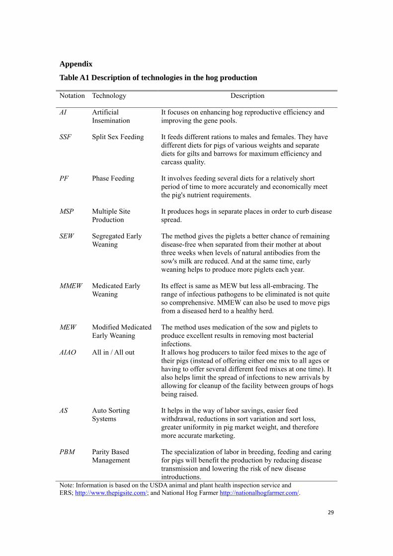
The data base also includes questions about if any of specific technologies was

used in individual worker’s farm. Hog production in the U.S. has experienced

tremendous technological innovations in advances in genetics, nutrition, housing and

handling equipment, veterinary and medical services, and management practices, and

the technology adoption contributes to productivity gain in recent decades (McBride

and Key, 2007). The appendix shows the technologies used in the hog farms between

1995 and 20052. The number of technologies adopted by the farm represents the

technology adoption intensity and can approximate the production complexity. In the

pork industry, large farms are found to favor technology adoption. 7.3 % of farms

adopted at most one of the advanced technologies and 70% of them produced fewer

than 5,000 pigs. In contrast, 8.8% of farms adopted all of technologies and more than

three quarters of them produced more than 25,000 pigs annually. On average, 4.5

technologies were used on a farm. Similarly, Technology is defined as a binary

variable, equal to one if more than five technologies were adopted, 0 otherwise.

Hog farms are categorized into four types according to production scale (D1 in

the notation in Section II) and technology adoption intensity (D2). Hence, there are

                                                              2 Two new technologies, Auto Sorting (AS) and Parity Based Management (PBM) are new technologies and were only available in the survey in 2005. Fewer than 30% of farms in 2005 adopted either of the two technologies. Because we control year fixed effect in our model and hog operators are exposed to the same technological shocks, different composition of technology across survey years will not significantly alter our results.  

  9

four combinations of farm types, (0, 0), (0, 1), (1, 0) and (1, 1), as shown in Table 13.

Farms of type (0, 0) are small and use no more than five technologies. Farms of type

(1, 1) are large and technologically intensive. The dataset enables us to estimate

treatment effects from size and technology adoption on wages after correcting

nonrandom assignment of workers into different types of firms. Finally, information

about worker’s social economic characteristics, wage level, work environment

evaluation and their health conditions is also available4. In particular, there are

several measures of worker skills or human capital: worker’s formal education,

previous working experience in the pork industry, tenure in the current farms and pork

production related childhood background.

Summary of statistics is shown in Table 1. Log of wage is highest in farms of

type (1, 1) and lowest in farms of type (0, 0). The wage differential in the two types

of farms is 0.47. The other two types of farms also pay more than (0, 0) type of farms.

Women are more likely to work in large farms but less likely to work in

technologically intensive farms. Workers in large and small farms are nearly equally

educated on average but more educated workers are more likely to work with more

advanced technologies. There is a stronger complementarity of worker schooling

with technology adoption than with farm size. Current work experience is

                                                              3 Not all hog farms are farrow-to-finish ones. Some, though a smaller proportion, of farms specialize in farrow-to-feeder or feeder-to-finish operations. Farm size of feeder-to-finish operations is expected to be smaller than that of feeder-to-finish operations. At the same time, technology adoption scenarios may also be different. It may be expected that farms raising feeder pigs to the market tend to have fewer technology options than would farms that raise piglets to finish pigs. If selection process for this particular farm type is significantly different from general farrow-to-finish farms, estimation of earning’s function and size wage premium will be biased. We replicated our analysis of model using a restricted sample that included only farrow-to-finish farms. We get qualitatively similar results and conclusions with those obtained with the full sample, and so our results are not driven by type of operations. 4 Location of farms are categorized into four regions: mid-west: IA, IL, IN, MN, MO, ND, NE, OH, SD, WI; northeast: CT,DC, DE, MA, MD, ME, MI, NH, NJ, NY, PA, RI, VT; southeast: AL,FL, GA, KY, LA, MS, NC, SC, TN, VA, WV; and west: AK, AR, AZ, CA,CO, HI, ID, KS, MT, NM, NV, OK, OR, TX, UT, WA, WY.  

  10

significantly skewed to small firms but not necessarily to high technology type of

farms. In contrast, previous experience of working in the pork industry is positively

related with both farm size and production complexity. Farm raised individuals tend

to work in small farms and they are possibly still working for family farms which are

generally small.

IV. Findings

We apply the methodology laid out in Section II to the sample of employees

on the US hog operations from 1995 to 2005. The formulation of earnings function

taking into account of selection on farm size and technology complexity enables us to

address two major concerns of the literature. The first concern has to do with the

importance of wage differentials in conditioning farm types. As shown in the

estimated standard earning’s function Table 2, even after controlling for worker’s

characteristics, firm’s location and year fixed effect, dummy variables Size and

Technology are significantly positively related with log of wage. Both size wage

premium and technology wage premium are significantly positive. However, as noted

above, potential endogeneity of Size and Technology may bias estimated coefficients

for the whole sample and for subsample of farms with different types in particular.

The second concern has to do with the treatment effect of the two important factors on

realized wages. After controlling for differential responses and characteristics,

treatment effect or impact of both Size and Technology may not be positive. In other

words, if equivalent workers are randomly assigned to different types of farms,

workers in large and technologically intensive farms may be paid less than their

counterparts. Whether selection is positive or negative will lead to different

conclusions about labor supply and labor demand in the pork industry. We present

empirical findings regarding the implied wage premium and offer possible

  11

explanations by citing several theories and presenting complementary evidence from

the survey questions. Then we make wage differentials decomposition.

A direct result from double selection: shrunk wage premium

Bi-variate probit model of double selection on Size and Technology is

presented in Table 3. The results are not particularly surprising, consistent with

general findings in the literature. Workers with higher education, workers with

previous relevant working experience and workers with hog-raising background are

more likely to work on large farms and on technologically advanced farms. The

correlation coefficient is 0.57, indicating that unobserved attributes on farms and

individuals significantly positively affect selection on farm size and technology

adoption intensity.

Based on this double selection regression above, inverse mills ratios for four

types of farms are obtained using equation (21) and added to the earnings function.

Estimation of equations (17) – (20) is shown in the last four columns of Table 2. We

find that earning’s functions are different across different types of hog farms. And at

least one of the coefficients of inverse mills ratios in each farm type is significantly

different from zero. The null hypothesis of no selection is rejected at the 5 percent

level of significance, indicating the existence of unobservables common to both the

selection and wage determination process. Both farm size and technology complexity

should be endogenously treated to remove the selection bias on wage premium

estimation. Because truncated mean of inverse mill’s ratios for farms with 0 or

0 are negative and positive for farms with 1 or 1, negative selection

coefficients for both four types of farms indicate that estimated wage premiums on

farm size and technology adoption intensity are reduced, compared to the wage gap

when workers are randomly allocated to four types of farms (Idson and Feaster, 1990).

  12

Several possibilities are proposed to account for the shrunk wage premiums.

Since our results are based on samples from pork production and technology adoption

is prevalent in today’s agricultural production, specific theories pertaining to

agricultural context are borrowed to justify the selection behaviors. However, we do

not exclude other potential interpretations.

Firstly, pork industry and generally agricultural industry are quite competitive and

small farms which do not benefit from economy of scale tend to easily exit the market.

Therefore, job stability and job security are worker’s big concerns. Workers who are

risk averse to job instability would like not to work in small farms. Large farms attract

workers because of higher profit margin and their dominant positions in the

competitive agricultural market. However, agricultural production is consistent with

the O-Ring theory where any mistake in a single stage from a series of production

process may lead to catastrophic failure (Kremer, 1993; Yu et al, 2009). Infection of

one pig may spread the diseases to the entire heard, driving profits to be negative.

Farms of larger scale are at greater stake and they are assumed to bear more risks.

Therefore, disease control is critically important for hog production. Large farms

have greater incentives to adopt several advanced technologies to curb spread of

diseases among pigs, such as Multiple Site Production, All-In-All-Out, Medicated

Early Weaning and Parity Based Management. From the perspective of hog workers,

farms that are less technologically intensive ensure a lower level of job security.

Secondly, workers in the agricultural industry are at increased risk for

occupational injuries, illnesses and even death, and the pork industry is no exception.

For example, hazardous gases released from decomposed manure and dust created

primarily from feeding practices put workers at risk for respiratory illness. Hog

farmers are found markedly tend to have higher risk in reduced hand strength and

  13

respiratory symptoms than non farmers (Hurley, et al, 2000). Workers, who are

increasingly likely to be hired from varying backgrounds, have become more aware of

existing occupational hazard than workers in the past. Farms with improved working

conditions, especially for air quality will attract workers who care about health

conditions.

We find that workers from either large farms or farms using complex

technologies reported a low level of dust and gas in the workplace and their

employer’s provision of protection on ear, eye and feet. As shown in Table 4, farms

that are large or technologically advanced, or both have better environment than (0, 0)

type of farms. Dust and gas levels are lower in those farms. At the same time, nearly

all of them provide dust masks or respirators and ear protection to their workers. They

are about 50% more likely to provide protection on ears, eyes and feet.

However, it is noteworthy that as far as the consequences of employer supply of

protection are concerned, not all of symptoms were reduced on large and

technologically complex farms compared to the (0, 0) type of farms. Workers in high

type farms are less likely to have throat irritation, chest tightness or wheezing chest,

but they do not have significantly reduced occurrences of other symptoms such as

phlegm, loess of hand strength or back pain. One of the reasons might be that

workers do not always wear the masks or other protective devices even they are

provided. Because working environment is believed to be better than other farms,

workers have reduced incentives in wearing protective devices. Adverse selection

problem occurs. The other reason is that some symptoms are hard to be avoided even

if some protective devices are provided, such as loss of hand strength and back pain.

Last but not the least, the findings also shed light on the wage policies in the hog

farms. The existence of positive size premium even after selection by workers is

  14

controlled can reflect wage policies by producers in multiple ways. Because large

farms using more technologies benefit from economy of scale, they would like to

share the productivity gain with employees. Alternatively, because the monitoring

cost in the large firms tends to be higher than that in the small firms, large farms

would rather set a wage premium as penalty for shirking, holding other characteristics

constant. Similarly, farms could use the agency models where workers care about

their pecuniary utility. It incurs monitoring cost to a less degree when evaluation of

relative performance among workers is used. However, large farms are cautious in

using relative performance to design wage structures. Highly skewed wage

distribution may induce sabotage among workers (Lazear, 1989). Again, because

agricultural production is consistent with the O-Ring theory, cooperation and

coordination among workers are increasingly important with farm size and production

complexity. Large farms tend to set average wages higher than those in small farms

but reduce the wage gap among workers therefore reduce potential sabotage. A

similar note has been made by Idson and Feaster (1990). Because large firms tend to

have formal work environment and would more highly value workers who fit well

into this environment, workers with “independence” and “individual drive” are less

likely to offer themselves to such formal work environment.

At the same time, people usually prefer fairness to inequality (Agell, 2004).

That is why pay is more compressed in large firms than in small firms. As shown in

Table 1, variance of log of real salaries is smaller in large farms no matter to what

extent advanced technologies are adopted. And in a reverse way, variance of log of

real salaries is smaller in technologically advanced farms no matter how many pigs

can be produced on those farms.

Decomposition of wage differentials

  15

In this subsection, we decompose wage differences between different types of

farms such that we can detect where the differentials are from and by how much they

are attributed to different factors. Wage differentials are decomposed in a similar way

of Idson and Feaster (1990) with a standard Oaxaca/Blinder method (Blinder 1973,

Oaxaca 1973). For the difference of expected logarithm wage in group j and group 1,

1, the wage differential is decomposed into several parts according to the

following equation,

(22) ′0.5 0.5 ′

The left hand side term of (22) is the raw logarithm wage differential (R). The three

terms in the right hand side are the endowment contribution to wage differential (E),

the changing coefficients’ contribution to wage differential, which could be further

decomposed into the part explained by the explanatory variables other than the

constant intercepts in wage equation (C) and the part absorbed in the intercepts (U),

and wage differential caused by self-selection (S).

Table 5 shows bilateral wage differentials’ decompositions among four types

of farms. Wage differences mainly lie in individual’s selectivity, responding

coefficients and intercepts. Differences in worker endowments contribute to the

smallest proportion of wage differentials. Furthermore, selection on size and

technology adoption intensity is not uniform. Differentials from selectivity are all

negative except for one case (S3 vs S2) and this is consistent with the selection effect

of reducing wage premium.

We find that the effect of reducing wage gap is comparably stronger for

selection on technology complexity than for selection on farm size. It can be seen

  16

from Table 5 that the magnitude of wage differentials from selectivity is larger than

for technology selection, holding farm size constant. For example, more than 70%

and 85% of the raw wage differences excluding selectivity for cases (S2 vs S1) and (S4

vs S3) are due to selection respectively. In contrast, no matter how many technologies

farms adopted, i.e., holding technology complexity constant, selectivity bias from

farm size is smaller. For example, only 44% and 79% of the raw wage differences

excluding selectivity for cases (S3 vs S1) and (S4 vs S2) are due to selection

respectively.

Therefore, it again justifies that technology adoption intensity be endogenous

in wage equation and extending the selection dimension be required to reduce the

estimation bias. As noted above, the majority of technologies used in the hog farms

are used to prevent diseases that are extremely important to profits. Furthermore, as

shown in Table 4, workers in high technology farms rated a better work environment

than those in large farms. Workers self select themselves into high technology farms

are more willing to compensate monetary income for working in a less hazardous

workplace which has low job loss risks at the same time.

Holding the number of technologies used on the farms constant, difference in

corresponding coefficients is the major component for wage differentials between

large and small farms ( case (S3 vs S1) and (S4 vs S2)). Large farms set higher

coefficients responding to worker’s characteristics and other firm attributes than small

farms. As stated above, large farms find it hard to monitor workers, setting bigger

coefficients could serve to prevent worker shirking. At the same time, knowing this,

potential workers are attracted to large size farms.

We also calculate some conditional wage gaps across different groups, which

could help us understand the potential wage benefit a worker could have by switching

  17

to different type of farms. The conditional wage gap for a worker who are observed

in the group j is the wage difference between the expected wage he has obtained in

group j and the expect wage he would have if he were selected into group k, where

, , 1, 2, 3 4. Explicitly,

(23) Δ , 1 | 1, ≡ 1

Table 6 shows the conditional wages for workers in (0, 0) farms and (1, 1)

type of farms in the upper and lower panel respectively. Because of existence of

dummy independent variables, worker characteristics are specified and evaluated at

some values or status such that conditional wages can be calculated. As shown in the

upper panel, a male worker in a typical type (0, 0) farm which was located in the west

received wage 5.08 in 2005. If he was employed in (0, 1) type of farms, his total

income will be 6.22, which comes from an increase in return to change in observables

Xβ, 1.36, and a decrease due to selection, 0.22. Both male and female employees in

farm of (0, 0) type experience wage increase from Xβ and wage decrease from

selection. The lower panel of Table 6 shows the wage decrease experienced by

female and male employees on farms of (1, 1) type if switching to other types of

farms. Again, wage drop is mainly due to change in Xβ. Selection difference is very

small. However, results from both panels indicate the same conclusion that selection

on technologies is bigger in magnitude than selection on farm size in explaining wage

differentials5.

V. Conclusion and discussion

Size wage premium is voluminously documented in literature. However, the                                                               5 In the upper panel, selection differentials due to switch from S1 to S2 and S4 are bigger in absolute value than those due to switch from S1 to S3. In the lower panel, selection differentials due to switch from S4 to S1 and S3 are bigger in absolute value than those due to switch from S4 to S2.

  18

current studies neglect the strong complementarity between firm size and technology

adoption, which has been found to have significant treatment effects on wages. This

study contributes to the literature by providing a better understanding of size wage

premium, labor supply decisions and wage policies. We include both size and

technology adoption in a double selection framework. We then apply the method to

estimate the wage structure in the US hog farms. It is found that correction for

selection on both size and technology adoption is required in wage equation and wage

premium for large farms or for technologically advanced farms are reduced after this

double selection is added into the earning’s function. Workers would rather

compensate pecuniary wages for better work environment and more secure job

stability, which is particularly highlighted in the agricultural industry. The effect of

reducing wage gap is comparably stronger for selection on technology complexity

than for selection on farm size.

Technology adoption has been paid a lot of attention to in agricultural

production because it can boost productivity and reduce cost. From this study we find

that worker’s belief on job stability and job itself induces them to self-select into

technologically advanced farms. Agricultural production has been experiencing rapid

technological innovation and farms become more and more specialized, which

motives a future research direction: whether wage premium is stable over time. This

study uses a cross sectional data base which provides a channel to the future research

once a panel is available.

A limitation of the study is that because respondents of surveys are subscribers

to the Magazine, they are not very representatives of all hog farm employees. And

because the propensity to respond to surveys may be larger for employees in larger

farms and lower for smaller farms, the sample under represents the small hog farms.

  19

Therefore, this study is an attempt to better understand the wage structure in hog

production based on a snapshot of hog farms. Availability of a new data base will

facilitate the consistent estimation of size and technology treatment effects on wages

of employee population in the US pork industry.

  20

Reference

[1] Abowd, John, Francis Kramarz and David Margolis, “High Wage Workers and

High Wage Firms,” Econometrica, 67 (1999), 251-337.

[2] Agell, Jonas. 2004. Why are small firms different? Manager’s views. Scandinavia

Journal of Economics 106(3): 437-452.

[3] Brown, Charles and James Medoff. 1989. The employer size-wage effect. Journal

of Political Economy: 1027-59.

[4] Heckman, James, 1979 Sample selection bias as a specification error,

Econometrica 47: 153-61.

[5] Huffman, Wallace. E. 2001. “Human Capital: Education and Agriculture,”

Handbook of Agricultural Economics, Volume 1, Part 1.

[6] Hurley, Terrance, James Kliebenstein and Peter Orazem. 2000. An analysis of

occupational health in pork production. American Journal of Agricultural

Economics 82: 323-333.

[7] Hurley, Terrance, James Kliebenstein and Peter Orazem. 2000. Structure of Wages

and Benefits in the U.S. Pork Industry. American Journal of Agricultural

Economics 81:144-163.

[8] Idson, Todd L & Feaster, Daniel J. 1990. A selectivity model of employer-size

wage differentials. Journal of Labor Economics: 8(1): 99-122.

[9] Key, Nigel and William McBride. 2007. The Changing Economics of U.S. Hog

Production. ERR-52, USDA, Economic Research Service.

[10] Kremer, Michael. 1993. The O-Ring Theory of Economic Development. The

Quarterly Journal of Economics 108: 551-575.

[11] Lazear Edward. 1989. Pay equality and industrial politics. Journal of Political

Economy 97: 561-580.

  21

  22

[12] Main, Brian and Barry Reilly. 1993. The Employer Size-Wage Gap: Evidence

for Britain. Economica 60 (238): 125-142.

[13] Moore, H. 1911. Laws of Wages: An Essay in Statistical Economics. New

York: Augustus.

[14] Oi, W. Y. and Idson, T.L. 1999. Farm size and wages. The Handbook of Labor

Economics.

[15] Reily, Kevin T. 1995. Human Capital and Information: the Employer Size Wage

Effect. Journal of Human Resources. 30: 1-18.

[16] Troske, Kenneth. 1999. Evidence on the Employer Size wage premium from

Worker-Establishment Matched Data. The Review of Economics and Statistics

81(1): 15-26.

[17] Tunali Insan. 1986. A General Structure for Models of Double Selection And

An Application To A Joint Migration/Earnings Process With Remigration,

Research in Labour Economics, volume 8, part B, pages 235-282.

[18] Willis, R and S. Rosen 1979. Education and Self-selection, Journal of

Political Economics, 87, S7-S36.

[19] Yu, Li and Terrance Hurly, James Kliebenstein and Peter Orazem. 2008. Firm

size, technical change and wages in the pork sector, 1990-2005. Iowa State

University Working Paper #08013.

[20] Yu, Li and Peter Orazem. 2008. Human Capital, Complex Technologies, Firm

Size and Wages: A Test of the O-Ring Production Hypotheses. Iowa State

University Working Paper #08029.

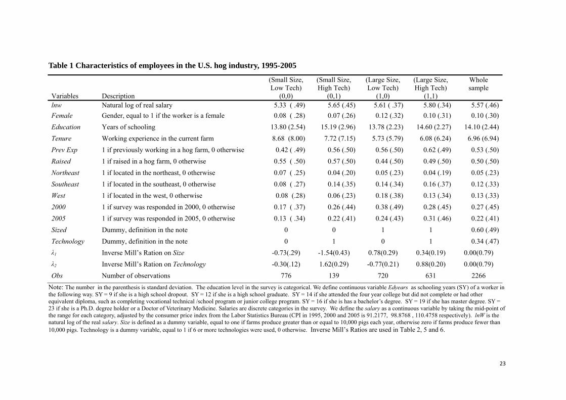
Table 1 Characteristics of employees in the U.S. hog industry, 1995-2005

Variables Description

(Small Size, Low Tech)

(0,0)

(Small Size, High Tech)

(0,1)

(Large Size, Low Tech)

(1,0)

(Large Size, High Tech)

(1,1)

Whole sample

lnw Natural log of real salary 5.33 ( .49) 5.65 (.45) 5.61 ( .37) 5.80 (.34) 5.57 (.46) Female Gender, equal to 1 if the worker is a female 0.08 ( .28) 0.07 (.26) 0.12 (.32) 0.10 (.31) 0.10 (.30) Education Years of schooling 13.80 (2.54) 15.19 (2.96) 13.78 (2.23) 14.60 (2.27) 14.10 (2.44) Tenure Working experience in the current farm 8.68 (8.00) 7.72 (7.15) 5.73 (5.79) 6.08 (6.24) 6.96 (6.94) Prev Exp 1 if previously working in a hog farm, 0 otherwise 0.42 ( .49) 0.56 (.50) 0.56 (.50) 0.62 (.49) 0.53 (.50) Raised 1 if raised in a hog farm, 0 otherwise 0.55 ( .50) 0.57 (.50) 0.44 (.50) 0.49 (.50) 0.50 (.50) Northeast 1 if located in the northeast, 0 otherwise 0.07 ( .25) 0.04 (.20) 0.05 (.23) 0.04 (.19) 0.05 (.23) Southeast 1 if located in the southeast, 0 otherwise 0.08 ( .27) 0.14 (.35) 0.14 (.34) 0.16 (.37) 0.12 (.33) West 1 if located in the west, 0 otherwise 0.08 (.28) 0.06 (.23) 0.18 (.38) 0.13 (.34) 0.13 (.33) 2000 1 if survey was responded in 2000, 0 otherwise 0.17 ( .37) 0.26 (.44) 0.38 (.49) 0.28 (.45) 0.27 (.45) 2005 1 if survey was responded in 2005, 0 otherwise 0.13 ( .34) 0.22 (.41) 0.24 (.43) 0.31 (.46) 0.22 (.41) Sized Dummy, definition in the note 0 0 1 1 0.60 (.49) Technology Dummy, definition in the note 0 1 0 1 0.34 (.47) λ1 Inverse Mill’s Ration on Size -0.73(.29) -1.54(0.43) 0.78(0.29) 0.34(0.19) 0.00(0.79) λ2 Inverse Mill’s Ration on Technology -0.30(.12) 1.62(0.29) -0.77(0.21) 0.88(0.20) 0.00(0.79) Obs Number of observations 776 139 720 631 2266

Note: The number in the parenthesis is standard deviation. The education level in the survey is categorical. We define continuous variable Edyears as schooling years (SY) of a worker in the following way. SY = 9 if she is a high school dropout. SY = 12 if she is a high school graduate. SY = 14 if she attended the four year college but did not complete or had other equivalent diploma, such as completing vocational technical /school program or junior college program. SY = 16 if she is has a bachelor’s degree. SY = 19 if she has master degree. SY = 23 if she is a Ph.D. degree holder or a Doctor of Veterinary Medicine. Salaries are discrete categories in the survey. We define the salary as a continuous variable by taking the mid-point of the range for each category, adjusted by the consumer price index from the Labor Statistics Bureau (CPI in 1995, 2000 and 2005 is 91.2177, 98.8768 , 110.4758 respectively). lnW is the natural log of the real salary. Size is defined as a dummy variable, equal to one if farms produce greater than or equal to 10,000 pigs each year, otherwise zero if farms produce fewer than 10,000 pigs. Technology is a dummy variable, equal to 1 if 6 or more technologies were used, 0 otherwise. Inverse Mill’s Ratios are used in Table 2, 5 and 6.

  23 

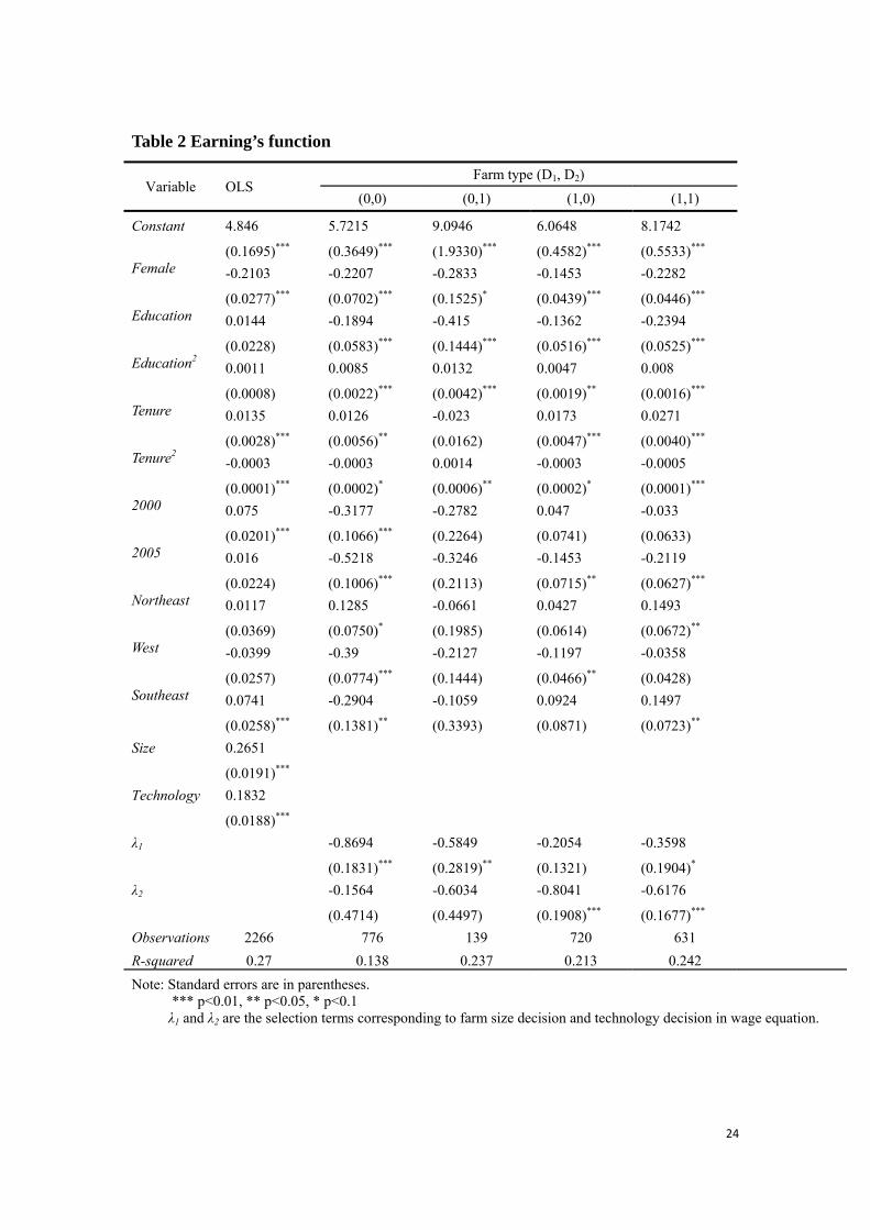
Table 2 Earning’s function

Variable OLS Farm type (D1, D2)

(0,0) (0,1) (1,0) (1,1)

Constant 4.846 5.7215 9.0946 6.0648 8.1742

(0.1695)*** (0.3649)*** (1.9330)*** (0.4582)*** (0.5533)*** Female -0.2103 -0.2207 -0.2833 -0.1453 -0.2282 (0.0277)*** (0.0702)*** (0.1525)* (0.0439)*** (0.0446)*** Education 0.0144 -0.1894 -0.415 -0.1362 -0.2394 (0.0228) (0.0583)*** (0.1444)*** (0.0516)*** (0.0525)*** Education2

0.0011 0.0085 0.0132 0.0047 0.008 (0.0008) (0.0022)*** (0.0042)*** (0.0019)** (0.0016)*** Tenure 0.0135 0.0126 -0.023 0.0173 0.0271 (0.0028)*** (0.0056)** (0.0162) (0.0047)*** (0.0040)*** Tenure2

-0.0003 -0.0003 0.0014 -0.0003 -0.0005 (0.0001)*** (0.0002)* (0.0006)** (0.0002)* (0.0001)*** 2000 0.075 -0.3177 -0.2782 0.047 -0.033 (0.0201)*** (0.1066)*** (0.2264) (0.0741) (0.0633) 2005 0.016 -0.5218 -0.3246 -0.1453 -0.2119 (0.0224) (0.1006)*** (0.2113) (0.0715)** (0.0627)*** Northeast 0.0117 0.1285 -0.0661 0.0427 0.1493 (0.0369) (0.0750)* (0.1985) (0.0614) (0.0672)** West -0.0399 -0.39 -0.2127 -0.1197 -0.0358 (0.0257) (0.0774)*** (0.1444) (0.0466)** (0.0428) Southeast 0.0741 -0.2904 -0.1059 0.0924 0.1497

(0.0258)*** (0.1381)** (0.3393) (0.0871) (0.0723)** Size 0.2651

(0.0191)*** Technology 0.1832

(0.0188)*** λ1 -0.8694 -0.5849 -0.2054 -0.3598

(0.1831)*** (0.2819)** (0.1321) (0.1904)* λ2 -0.1564 -0.6034 -0.8041 -0.6176

(0.4714) (0.4497) (0.1908)*** (0.1677)*** Observations 2266 776 139 720 631 R-squared 0.27 0.138 0.237 0.213 0.242 Note: Standard errors are in parentheses. *** p<0.01, ** p<0.05, * p<0.1 λ1 and λ2 are the selection terms corresponding to farm size decision and technology decision in wage equation.  

24  

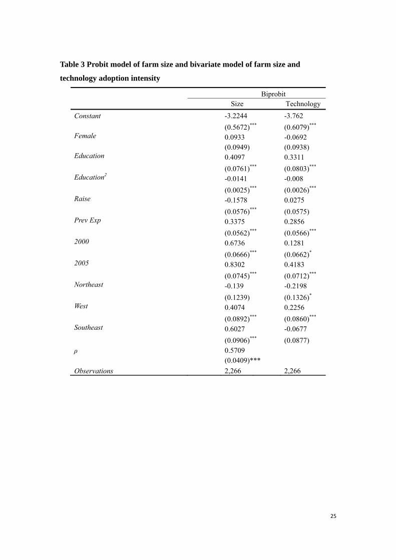
Table 3 Probit model of farm size and bivariate model of farm size and

technology adoption intensity

Biprobit Size Technology

Constant -3.2244 -3.762

(0.5672)*** (0.6079)*** Female 0.0933 -0.0692 (0.0949) (0.0938) Education 0.4097 0.3311 (0.0761)*** (0.0803)*** Education2

-0.0141 -0.008 (0.0025)*** (0.0026)*** Raise -0.1578 0.0275 (0.0576)*** (0.0575) Prev Exp

0.3375 0.2856 (0.0562)*** (0.0566)*** 2000 0.6736 0.1281 (0.0666)*** (0.0662)* 2005 0.8302 0.4183 (0.0745)*** (0.0712)*** Northeast -0.139 -0.2198 (0.1239) (0.1326)* West 0.4074 0.2256 (0.0892)*** (0.0860)*** Southeast 0.6027 -0.0677 (0.0906)*** (0.0877) ρ 0.5709 (0.0409)*** Observations 2,266 2,266

25  

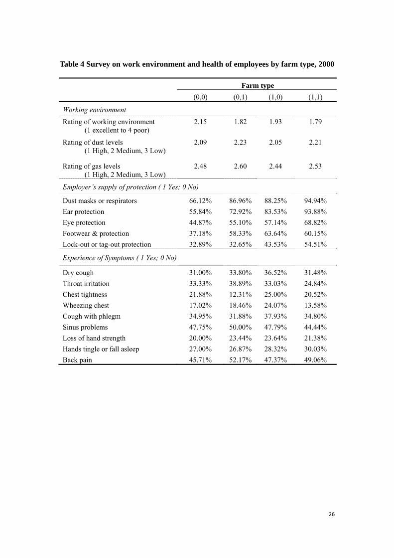
Table 4 Survey on work environment and health of employees by farm type, 2000

Farm type

(0,0) (0,1) (1,0) (1,1)

Working environment Rating of working environment (1 excellent to 4 poor)

2.15 1.82 1.93 1.79

Rating of dust levels (1 High, 2 Medium, 3 Low)

2.09 2.23 2.05 2.21

Rating of gas levels (1 High, 2 Medium, 3 Low)

2.48 2.60 2.44 2.53

Employer’s supply of protection ( 1 Yes; 0 No)

Dust masks or respirators 66.12% 86.96% 88.25% 94.94% Ear protection 55.84% 72.92% 83.53% 93.88% Eye protection 44.87% 55.10% 57.14% 68.82% Footwear & protection 37.18% 58.33% 63.64% 60.15% Lock-out or tag-out protection 32.89% 32.65% 43.53% 54.51%

Experience of Symptoms ( 1 Yes; 0 No)

Dry cough 31.00% 33.80% 36.52% 31.48% Throat irritation 33.33% 38.89% 33.03% 24.84% Chest tightness 21.88% 12.31% 25.00% 20.52% Wheezing chest 17.02% 18.46% 24.07% 13.58% Cough with phlegm 34.95% 31.88% 37.93% 34.80% Sinus problems 47.75% 50.00% 47.79% 44.44% Loss of hand strength 20.00% 23.44% 23.64% 21.38% Hands tingle or fall asleep 27.00% 26.87% 28.32% 30.03% Back pain 45.71% 52.17% 47.37% 49.06%

26  

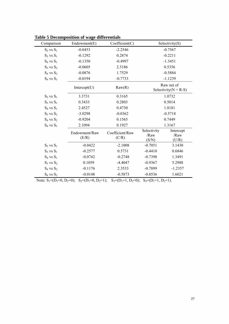
Table 5 Decomposition of wage differentials Comparison Endowment(E) Coefficient(C) Selectivity(S)

S2 vs S1 -0.0453 -2.2546 -0.7567 S3 vs S1 -0.1292 0.2874 -0.2211 S4 vs S1 -0.1350 -0.4997 -1.3451 S3 vs S2 -0.0605 2.5186 0.5356 S4 vs S2 -0.0876 1.7529 -0.5884 S4 vs S3 -0.0194 -0.7733 -1.1239

Intercept(U) Raw(R) Raw net of Selectivity(N = R-S)

S2 vs S1 3.3731 0.3165 1.0732 S3 vs S1 0.3433 0.2803 0.5014 S4 vs S1 2.4527 0.4730 1.8181 S3 vs S2 -3.0298 -0.0362 -0.5718 S4 vs S2 -0.9204 0.1565 0.7449 S4 vs S3 2.1094 0.1927 1.3167

Endowment/Raw(E/R)

Coefficient/Raw (C/R)

Selectivity /Raw (S/N)

Intercept /Raw (U/R)

S2 vs S1 -0.0422 -2.1008 -0.7051 3.1430 S3 vs S1 -0.2577 0.5731 -0.4410 0.6846 S4 vs S1 -0.0742 -0.2748 -0.7398 1.3491 S3 vs S2 0.1059 -4.4047 -0.9367 5.2988 S4 vs S2 -0.1176 2.3533 -0.7899 -1.2357 S4 vs S3 -0.0148 -0.5873 -0.8536 1.6021

Note: S1=(D1=0, D2=0); S2=(D1=0, D2=1); S3=(D1=1, D2=0); S4=(D1=1, D2=1).

27  

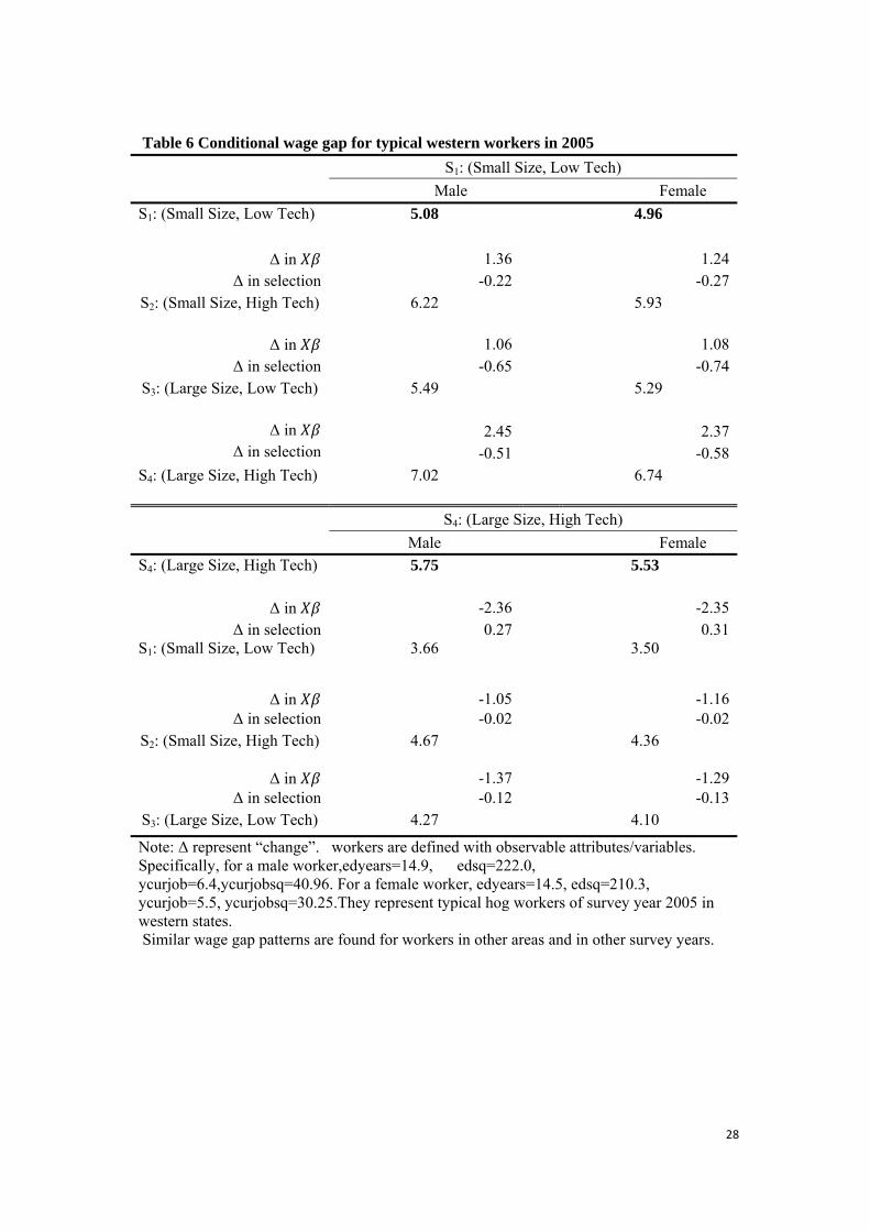
Table 6 Conditional wage gap for typical western workers in 2005 S1: (Small Size, Low Tech) Male Female

S1: (Small Size, Low Tech) 5.08 4.96

Δ in 1.36 1.24 Δ in selection -0.22 -0.27

S2: (Small Size, High Tech) 6.22 5.93

Δ in 1.06 1.08 Δ in selection -0.65 -0.74

S3: (Large Size, Low Tech) 5.49 5.29

Δ in 2.45 2.37 Δ in selection -0.51 -0.58

S4: (Large Size, High Tech) 7.02 6.74

S4: (Large Size, High Tech) Male Female

S4: (Large Size, High Tech) 5.75 5.53

Δ in -2.36 -2.35 Δ in selection 0.27 0.31

S1: (Small Size, Low Tech) 3.66 3.50

Δ in -1.05 -1.16 Δ in selection -0.02 -0.02

S2: (Small Size, High Tech) 4.67 4.36

Δ in -1.37 -1.29 Δ in selection -0.12 -0.13

S3: (Large Size, Low Tech) 4.27 4.10

Note: Δ represent “change”. workers are defined with observable attributes/variables. Specifically, for a male worker,edyears=14.9, edsq=222.0, ycurjob=6.4,ycurjobsq=40.96. For a female worker, edyears=14.5, edsq=210.3, ycurjob=5.5, ycurjobsq=30.25.They represent typical hog workers of survey year 2005 in western states. Similar wage gap patterns are found for workers in other areas and in other survey years.

28  

29  

Appendix

Table A1 Description of technologies in the hog production Notation Technology Description

AI Artificial Insemination

It focuses on enhancing hog reproductive efficiency and improving the gene pools.

SSF Split Sex Feeding It feeds different rations to males and females. They have different diets for pigs of various weights and separate diets for gilts and barrows for maximum efficiency and carcass quality.

PF Phase Feeding It involves feeding several diets for a relatively short period of time to more accurately and economically meet the pig's nutrient requirements.

MSP Multiple Site Production

It produces hogs in separate places in order to curb disease spread.

SEW Segregated Early Weaning

The method gives the piglets a better chance of remaining disease-free when separated from their mother at about three weeks when levels of natural antibodies from the sow's milk are reduced. And at the same time, early weaning helps to produce more piglets each year.

MMEW Medicated Early Weaning

Its effect is same as MEW but less all-embracing. The range of infectious pathogens to be eliminated is not quite so comprehensive. MMEW can also be used to move pigs from a diseased herd to a healthy herd.

MEW Modified Medicated Early Weaning

The method uses medication of the sow and piglets to produce excellent results in removing most bacterial infections.

AIAO All in / All out It allows hog producers to tailor feed mixes to the age of their pigs (instead of offering either one mix to all ages or having to offer several different feed mixes at one time). It also helps limit the spread of infections to new arrivals by allowing for cleanup of the facility between groups of hogs being raised.

AS Auto Sorting Systems

It helps in the way of labor savings, easier feed withdrawal, reductions in sort variation and sort loss, greater uniformity in pig market weight, and therefore more accurate marketing.

PBM Parity Based Management

The specialization of labor in breeding, feeding and caring for pigs will benefit the production by reducing disease transmission and lowering the risk of new disease introductions.

Note: Information is based on the USDA animal and plant health inspection service and ERS; http://www.thepigsite.com/; and National Hog Farmer http://nationalhogfarmer.com/.