Force-based Finite Element forLarge Displacement Inelastic Analysis of Frames

by

Remo Magalhães de Souza

Eng. Civil (Federal University of Pará, Brazil) 1990M.Sc. (Pontifical Catholic University – Rio de Janeiro, Brazil) 1992

A dissertation submitted in partial satisfaction of the

requirements for the degree of

Doctor of Philosophy

in

Engineering - Civil and Environmental Engineering

in the

GRADUATE DIVISION

of the

UNIVERSITY OF CALIFORNIA, BERKELEY

Committee in charge:

Professor Filip C. Filippou, ChairProfessor Robert L. Taylor

Professor Gregory L. FenvesProfessor Panayiotis Papadopoulos

Fall 2000

The dissertation of Remo Magalhães de Souza is approved:

Date

University of California, Berkeley

Fall 2000

Force-based Finite Element forLarge Displacement Inelastic Analysis of Frames

Copyright 2000

by

Remo Magalhães de Souza

1

Abstract

Force-based Finite Element forLarge Displacement Inelastic Analysis of Frames

by

Remo Magalhães de Souza

Doctor of Philosophy in Engineering - Civil and Environmental Engineering

University of California, Berkeley

Professor Filip C. Filippou, Chair

This dissertation presents a force-based formulation for inelastic large displacement

analysis of planar and spatial frames, and its consistent numerical implementation in a

general-purpose finite element program.

The main idea of the method is to use force interpolation functions that strictly

satisfy equilibrium in the deformed configuration of the element. The appropriate

reference frame for establishing these force interpolation functions is a basic coordinate

system without rigid body modes. In this system, the element tangent stiffness is non-

singular and can be obtained by inversion of the flexibility matrix.

The formulation is derived from a geometrically nonlinear form of the Hellinger-

Reissner potential, with a nonlinear strain-displacement relation that corresponds to a

degenerated form of Green-Lagrange strains.

Although the adopted kinematics is based on the assumption of moderately large

2

deformations along the element, rigid body displacements and rotations can be arbitrarily

large. This is accomplished with the use of the corotational formulation, in which rigid

body modes are separated from element deformations by attaching a reference coordinate

system (the basic system) to the element as it deforms. The transformations of

displacements and forces between the basic and the global systems are determined with

no simplifications regarding the magnitude of the rigid body motion. The non-vectorial

nature of rotations in space is handled consistently, through the representation in terms of

rotation matrices, rotational vectors and unit quaternions.

A new algorithm for the determination of the element resisting forces and tangent

stiffness matrix for given trial displacements is proposed. The iterative and non-iterative

forms of the algorithm are presented, generalizing earlier procedures for this class of

force-based elements.

Several planar and spatial problems are studied in order to validate the proposed

element. With the present formulation, only one element per structural member is

necessary for the analysis of problems with large rigid body rotations and moderate

deformations. Furthermore, finite strain problems can also be solved with the proposed

formulation, provided that the structural member is subdivided into smaller elements.

_________________________________

Professor Filip C. Filippou, Chair

i

Aos meus pais,

Pedro e Franci

(To my parents,

Pedro and Franci)

ii

Table of Contents

List of Figures....................................................................................................... vi

List of Tables ........................................................................................................ ix

Acknowledgments ................................................................................................. x

Chapter 1 Introduction ........................................................................................ 1

1.1 Material or physical nonlinearity .................................................................. 1

1.2. Geometric nonlinearity ................................................................................ 3

1.3 Displacement and force-based elements....................................................... 4

1.4 Literature survey ........................................................................................... 6

1.4.1 Displacement-based elements................................................................ 6

1.4.2 Force-based elements............................................................................. 7

1.4.3 Corotational formulation...................................................................... 10

1.4.4 Geometrically exact formulations........................................................ 11

1.5 Objectives and scope................................................................................... 12

Chapter 2 Plane Frame Element Formulation................................................. 16

2.1 Coordinate systems ..................................................................................... 16

2.2 Kinematic hypothesis.................................................................................. 19

2.3 Variational formulation............................................................................... 22

iii

2.4 Equilibrium equations................................................................................. 27

2.5 Weak form of the compatibility equation ................................................... 29

2.6 Section constitutive relations ...................................................................... 31

2.7 Consistent flexibility matrix ....................................................................... 34

2.8 Curvature-based displacement interpolation (CBDI) ................................. 36

2.9 Corotational formulation............................................................................. 40

2.9.1 Element (initial) local frame ................................................................ 41

2.9.2 Basic frame or displaced local frame................................................... 42

2.9.3 Transformation of displacements between coordinate systems........... 44

2.9.4 Transformation of forces...................................................................... 47

2.9.5 Tangent stiffness matrix in the global system...................................... 51

Chapter 3 Large Rotations................................................................................. 55

3.1 Rotation Matrix – Rodrigues Formula........................................................ 55

3.2 Extraction of the rotational vector from the rotation matrix....................... 62

3.3 Euler parameters and normalized quaternions............................................ 63

3.4 Compound rotations.................................................................................... 65

3.5 Extraction of the unit quaternion from the rotation matrix......................... 66

3.6 The variation of the rotation matrix ............................................................ 71

3.7 Rotation of a triad via the smallest rotation ................................................ 72

Chapter 4 Space Element Formulation............................................................. 74

4.1 Coordinate systems ..................................................................................... 74

4.2 Kinematic hypothesis.................................................................................. 76

4.3 Variational formulation............................................................................... 79

iv

4.4 Equilibrium equations................................................................................. 82

4.5 Weak form of the compatibility equation ................................................... 84

4.6 Section constitutive relations ...................................................................... 87

4.6.1 Simplified section constitutive relation ............................................... 90

4.7 Consistent flexibility matrix ....................................................................... 91

4.8 Curvature-based displacement interpolation (CBDI) ................................. 93

4.9 Corotational formulation............................................................................. 96

4.9.1 Element (initial) local frame ................................................................ 97

4.9.2 Element degrees of freedom in the global system ............................... 98

4.9.3 Nodal triads.......................................................................................... 99

4.9.4 Basic frame or displaced local frame................................................. 100

4.9.5 Rotation vectors expressed with respect to the basic frame .............. 105

4.9.6 Transformation of displacements between coordinate systems......... 107

4.9.7 Transformation of forces.................................................................... 109

4.9.8 Tangent stiffness matrix in the global system.................................... 114

Chapter 5 Element State Determination......................................................... 119

5.1 Non-iterative form of the state determination procedure.......................... 121

5.1.1 Element level of the state determination procedure........................... 121

5.1.2 Section level of the state determination procedure ............................ 124

5.2 Iterative form of the state determination procedure.................................. 135

5.3 Computer implementation of the corotational formulation ...................... 137

5.3.1 Planar case ......................................................................................... 138

5.3.2 Spatial case ........................................................................................ 139

v

5.4 Update of history variables ....................................................................... 143

Chapter 6 Numerical Examples....................................................................... 144

6.1 Williams toggle frame............................................................................... 145

6.2 Simply supported beam with uniform load............................................... 147

6.3 Cantilever beam with vertical load at the tip ............................................ 149

6.4 Cantilever beam under a moment at the tip .............................................. 152

6.5 Lee’s frame ............................................................................................... 155

6.6 El-Zanaty portal frame.............................................................................. 160

6.7 Framed dome ............................................................................................ 162

6.8 Cantilever right-angled frame under end-load.......................................... 165

6.9 Hinged right-angled frame under applied end moments........................... 167

6.10 Two-story three-dimensional frame........................................................ 170

6.11 Six-story three-dimensional frame.......................................................... 172

Chapter 7 Conclusions...................................................................................... 175

References.......................................................................................................... 181

Appendix A Derivation of the CBDI Influence Matrix ................................. 190

Appendix B Rotation of a Triad via the Smallest Rotation .......................... 193

Appendix C Derivation of the Spatial Geometric Stiffness Matrix.............. 196

vi

List of Figures

Figure 2.1 Element with reference to the global coordinate system (X, Y). ...................17

Figure 2.2 Global and basic coordinate systems. ...........................................................18

Figure 2.3 Displacement field of the beam. ...................................................................20

Figure 2.4 Basic system indicating displacement fields and corresponding

boundary conditions......................................................................................25

Figure 2.5 Element local (initial) frame. ........................................................................42

Figure 2.6 Element basic (displaced) frame...................................................................44

Figure 2.7 Basic displacements. .....................................................................................45

Figure 2.8 Transformation of forces between global and basic coordinates..................48

Figure 3.1 Rotation of a vector in space.........................................................................56

Figure 3.2 Spurrier’s algorithm for the extraction of the unit quaternion from

the rotation matrix.........................................................................................69

Figure 3.3 Pseudo code for the extraction of the rotational vector from the unit

quaternion .....................................................................................................71

Figure 4.1 Basic coordinate system in space..................................................................75

Figure 4.2 Basic coordinate system................................................................................81

Figure 4.3 Spatial element local (initial) frame..............................................................98

Figure 4.4 Nodal triads at the deformed configuration. ...............................................100

Figure 4.5 Element basic (displaced) frame in space...................................................101

Figure 5.1 Element level of the non-iterative state determination procedure. .............122

vii

Figure 5.2 Section level of the state determination procedure .....................................131

Figure 5.3 Element level of the iterative state determination procedure......................135

Figure 5.4 Pseudo code of the iterative state determination procedure........................137

Figure 6.1 Williams toggle frame with section analyzed by Chan (1998)...................145

Figure 6.2 Equilibrium paths for toggle frame.............................................................146

Figure 6.3 Simply supported beam with uniform load.................................................148

Figure 6.4 Load-displacement curves for simply supported beam ..............................149

Figure 6.5 Cantilever beam with vertical load at the tip. .............................................150

Figure 6.6 Equilibrium paths for the cantilever problem. ............................................151

Figure 6.7 Cantilever subjected to end moment...........................................................152

Figure 6.8 Relative displacements for beam subjected to end moment. ......................154

Figure 6.9 Deformed shapes for the cantilever beam, corresponding to each

load step. .....................................................................................................155

Figure 6.10 Lee’s frame. ................................................................................................156

Figure 6.11 Equilibrium paths for Lee’s frame (with coarser discretization). ...............157

Figure 6.12 Equilibrium paths for Lee’s frame (with finer discretization). ...................158

Figure 6.13 Deformed shapes (to scale) of Lee’s frame for the finer

discretization, considering elastic material. ................................................159

Figure 6.14 El-Zanaty portal frame................................................................................160

Figure 6.15 Load-displacement curves for El-Zanaty frame. ........................................161

Figure 6.16 Framed dome. .............................................................................................163

Figure 6.17 Load-displacement curves for framed dome...............................................164

Figure 6.18 Right-angled frame under end load.............................................................165

viii

Figure 6.19 Load-displacement curve for right-angled frame under end load...............167

Figure 6.20 Right-angled frame under applied end moments. .......................................168

Figure 6.21 Load-displacement curve for right-angled frame under end moments. ......169

Figure 6.22 Two-story frame..........................................................................................171

Figure 6.23 Load-displacement curve for two-story frame............................................172

Figure 6.24 Six-story space frame..................................................................................173

Figure 6.25 Load-displacement curve for six-story frame. ............................................174

ix

List of Tables

Table 5.1 Computer implementation of the planar corotational formulation. ............ 138

Table 5.2 Computer implementation of the spatial corotational formulation............. 142

Table 6.1 Convergence rate for cantilever problem at load step 6. ............................ 152

x

Acknowledgments

I wish to express my appreciation to Prof. Filip C. Filippou, my research advisor

and chair of the dissertation committee, for his precious support during my doctoral

program and guidance in this work. I also wish to thank Prof. Filippou for the knowledge

and wisdom transmitted about the several aspects of academic life. It has been a great

pleasure to have this long relationship with such a friendly and enthusiastic teacher.

I also wish to thank the other members of my dissertation committee, Prof. Robert

L. Taylor, Prof. Gregory L. Fenves and Prof. Panayiotis Papadopoulos for the important

discussions and comments related to this study. More specifically, I would like to thank

Prof. Robert L. Taylor for his valuable insight on the derivation of the proposed element

formulation using the Hellinger-Reissner functional, and to thank Prof. Gregory L.

Fenves for his support and helpful suggestions related to the computer implementation of

nonlinear frame elements in an objected-oriented programing framework. Their effort

reading and revising this dissertation is greatly appreciated.

I would like to express my deepest gratitude to my wife, Virginia, for her

encouragement, sacrifice and love. I will never be able to thank her enough for leaving

her career and family in Brazil, to accompany me during my doctoral studies.

Accomplishing this arduous task without her support would be virtually impossible. I am

blessed for having such a wonderful and lovely person standing by my side during all

those years.

I wish I knew how to thank my three-year old son, Pedro, for his immeasurable

xi

help with my studies. I am thankful for him showing me, every day, the joy and

happiness of being a father. He is the most important source of energy and enthusiasm

that I have. In addition, his concerns about the conclusion of this dissertation are

gratefully acknowledged.

I am thankful for the immense support and love received from my parents Pedro

and Franci during my entire life. Their effort in raising and educating me and my

brothers, and the patience in waiting for me to complete my graduate studies and to go

back home are sincerely appreciated.

I am also grateful for the incentive and love received from my other relatives in

Belém-Brazil, Ronan, Rômulo, Nirvia, Rominho, Pilar, Adiléia, Rev. Stélio, Gérson,

Zeneide, Enã, Estélio, and Selma. Even being so far away they helped me in many

different ways. Their help was really important for the completion of this program.

I also would like to thank my “family” in the United States: Amanda, Fernanda,

Paulo, Andréa, Márcia, André, Lucas, Ana Flávia, Reinaldo Gregori, Rafael, Liliana,

Sérgio, Thaís, Armando, and Reinaldo Garcia, for the great moments lived together. I am

sure that the friendship that was born in Berkeley will grow and last forever.

I am indebted to the fellow students, faculty and staff members in the University

of California at Berkeley who contributed to the conclusion of my doctoral studies.

Special thanks go to Frank McKenna and Michael Scott for their help with the computer

implementation of this research work; to Ashraf Ayoub, Ignacio Romero, David Ehrlich,

Prashanth Vijalapura, and Mehrdad Sasani, for the helpful discussions about

computational mechanics and nonlinear structural analysis; to Prof. Khalid Mosalam,

Prof. Francisco Armero and Prof. Keith Miller for serving in my qualifying examination

xii

committee (in addition to Prof. Filippou, and Prof. Fenves); to Mari Cook for the help

with academic matters since the beginning of my application process.

I would like to thank the faculty members of the Civil Engineering Department of

the Universidade Federal do Pará (Federal University of Pará) for the approval of my

leave of absence, such that I could attend this doctoral program. I am especially thankful

to Prof. José Perilo da Rosa Neto, for his help with administrative matters related to my

absence, and for the constant motivation received during my undergraduate and graduate

studies in civil engineering.

Financial support for these studies were provided by the Ministry of Education of

Brazil, through the federal agency CAPES. This research work was also in part supported

by the National Science Foundation, through the Pacific Earthquake Engineering

Research (PEER) Center. This financial support is gratefully acknowledged.

1

Chapter 1Introduction

This work addresses the analysis of frames with material and geometric nonlinearity. A

frame with slender members under load conditions causing deformations past the elastic

limit of the material is the typical case of problems where both effects need to be

considered.

1.1 Material or physical nonlinearity

In the analysis of frame elements the material nonlinearity is defined at the cross-section

level. Basically, there are two approaches for representing section constitutive behavior:

a) Utilization of a direct relation between stress resultants (such as axial force and

bending moments) and generalized strains (such as a reference axial strain and

curvature); b) Integration of material stress-strain relations defined at the material point

level, over the area of the cross-section.

The first approach has the disadvantage of requiring specialized force-

deformation relations for different types of cross-section. Although this is not a severe

drawback in the case of steel frames, where standard shapes are usually employed, this

approach is not well suited to reinforced concrete frames, due to the total variability of

possible cross-section designs. In addition, the coupled response between stress resultants

(e.g., axial force and bending moment), even when a uniaxial stress state is assumed,

2

introduces greater complexity in the relation. To account for the coupled behavior, this

approach is usually based on the theory of plasticity and employs a yield-surface function

in terms of stress resultants. Another disadvantage of this method consists in the

difficulty of representing precisely partial yielding of the cross-section.

Regarding the second approach, very accurate constitutive relations are obtained

at the expense of using a refined grid to numerically evaluate integrals over the cross-

sections. As a large number of sampling points may be necessary, the computational

effort to perform the numerical integration, and the storage of history variables associated

with each of these points, usually render the method more computationally expensive

than the force-deformation approach, particularly for complex space structures with many

elements. However, the advantages of the method outweigh this drawback in many

aspects. The most important advantage is its ability to handle general types of cross-

section, a feature that is especially convenient in the analysis of reinforced concrete

frames. Furthermore, partial yielding and cracking of the cross-section can be represented

in a simple and accurate manner.

This approach is particularly advantageous when the commonly adopted

assumption of uniaxial stress state at the material points of the cross-section is made. In

this situation, the method is usually called ‘fiber-discretization’ technique. For this type

of stress-state, high accuracy is achieved, and great flexibility is possible in terms of the

material constitutive relations that can be represented. Many strain hardening laws with

different loading/unloading criteria, and residual or thermal stresses can be easily

considered with this approach. For instance, representing a reinforced concrete (shear

free) section, with realistic material models, becomes very simple.

3

Regarding the spreading of plasticity along the element, this effect can be

accounted for, very accurately, using the so-called ‘plastic zone’ methods, which involve

numerical integration over the element length. Alternatively, the approximate ‘plastic-

hinge’ approach can be used, but depending on the structure under consideration the

results can be very unconservative. The plastic-hinge approach, however, is appropriate

in the presence of softening material behavior, which limits the size of the plastic-zones

to small concentrated regions.

1.2. Geometric nonlinearity

The numerical solution of geometrically non-linear frame problems is usually based on

either a total Lagrangian, an updated Lagrangian or a co-rotational formulation (or

combinations, as described later). These kinematic formulations are similar for finite

deformation problems in continuum mechanics, with the only difference being the

reference configuration system adopted to describe the motion of the body. However, for

structural elements based on approximate geometrically nonlinear theories, the results of

the different formulations may not be the same.

In the total Lagrangian formulation, the reference system is the original

undeformed element configuration. In the updated Lagrangian formulation, the last

computed deformed configuration is adopted as the reference system. The corotational

formulation separates rigid-body modes from local deformations, using as reference, a

single coordinate system that continuously translates and rotates with the element as the

deformation proceeds.

4

As the corotational formulation is employed in the present work, a brief literature

review of this approach is given in section 1.4.3.

Although the treatment of geometrically nonlinear effects in large-displacement

planar problems may be a complex subject itself, the extension of bidimensional

formulations to three dimensions is by no means trivial for this type of problem. This is

due to the non-vectorial nature of large rotations in space.

In geometrically linear problems, rotations are considered infinitesimal, and

therefore can be treated as vectors. However, in spatial problems with large displace-

ments, rotations are not vector entities, as can be easily confirmed by verifying that the

commutative property of vectors does not hold for large rotations in space. This can be

observed by imposing a sequence of rotations to a body, around two or three orthogonal

axes, and concluding that the final position of the body depends on the sequence of the

imposed rotations.

1.3 Displacement and force-based elements

Most of the research work on geometric and material nonlinear analysis of frames is

based on the displacement method, employing either a total, updated lagrangian, or

corotational formulation. In these studies, usually based on finite element method

concepts, nonlinear strain-displacement relations are considered, and polynomial

interpolation functions are assumed for the displacement fields. Due to the adoption of

assumed interpolation functions, discretization with several elements is required to model

each structural member of the frame. This is necessary in order to capture the actual

5

variation of large deformations along the member length. The need of several elements

per member, and consequently of a great number of degrees of freedom, results in

reduced computational efficiency for most of the traditional displacement-based finite

elements.

In order to avoid the discretization of frame members, an alternative procedure

consists in the use of elements with the plastic-hinge concept and second order beam-

column theory, such that only one element per member can be used. However, depending

on the characteristics of the structure, these elements can be rather inaccurate when the

spread of plasticity effect is relevant. The use of higher order polynomials for the

displacement interpolation functions is an alternative approach.

Another solution is the utilization of force-based (or flexibility-based)

formulations, in which equilibrium is satisfied strictly. If non-linear geometric effects are

neglected, exact interpolation functions can be readily established. For example, in the

absence of distributed loads, the bending moment variation along a frame element is

always linear, although the curvature distribution can be very irregular due to the

formation of plastic zones at the element ends. In the presence of moderately large

deformations, the force interpolation functions, although not necessarily exact, provide

means for a better representation of the stiffness variation along the beam than the

traditional approach with assumed displacement functions.

It is important to emphasize that exact force distributions are easily determined

for one-dimensional elements only. In case of continuum elements, exact force

interpolation functions are not available. Therefore, force-based formulations seem

especially suited for the nonlinear analysis of frames.

6

1.4 Literature survey

Nonlinear structural analysis has been the subject of very extensive research. More

specifically, several studies on the nonlinear behavior of frames have been conducted

over the last four decades. As the number of these studies is vast, only a few of the works

that include nonlinear geometric effects are listed herein. Most of the proposed elements

are based on the displacement formulation, with only a few based on force or mixed

formulations.

Special attention is given in this review to works related to force-based elements

and to the corotational formulation. Some studies based on the displacement formulation

are listed first, without significant detail. A more detailed description of force-based

formulation in the literature is then given. Following this, a short description of the

corotational approach is presented, listing some of the relevant works in this field.

Finally, a brief description of works related to the so-called geometric exact theories is

provided.

1.4.1 Displacement-based elements

The development of elements for elastic nonlinear analysis of frames started in the

sixties. Some of the earliest papers on elastic nonlinear analysis are, for instance, Argyris

et al. (1964) and Connor et al. (1968). Early studies considering both material and

geometric nonlinear effects are, for example, Korn and Galambos (1968) and Alvarez and

Birnstiel (1969).

One important early study on large displacement analysis of frame structures is

7

the paper by Bathe and Bolourchi (1979), which presented an updated Lagrangian and a

total Lagrangian formulation for three-dimensional beam elements derived from the

principles of continuum mechanics.

The second order inelastic analysis of frame structures, particularly of steel

buildings, was the subject of much research work during the following years. Some more

recent publications in this field, proposing new elements for practical analysis/design of

steel frames, are for instance El-Zanaty et al. (1980), El-Zanaty and Murray (1983),

White (1985), King et al. (1992), Ziemian et al. (1992), Liew et al. (1993), Attalla et al.

(1994), King and Chen (1994), Chen and Chan (1995), Barsan and Chiorean (1999), and

Liew et al. (2000).

Other publications on large displacement inelastic frame analysis, not specifically

for steel frames, are Cichon (1984), Simo et al. (1984), Tuomala and Mikkola (1984),

Nedergaard and Pedersen (1985), Chan (1988), Gendy and Saleeb (1993), Ovunc and

Ren (1996), Park and Lee (1996), and Waszczyszyn and Janus-Michalska (1998).

Although some of the elements proposed in the above studies can be adapted for

reinforced concrete structures, the bibliography on geometrically and materially nonlinear

frame elements for this specific type of structure is scarcer. Some examples are Aldstedt

and Bergan (1978), and Marí et al. (1984).

1.4.2 Force-based elements

Only a few elements based on the force approach have been proposed for the nonlinear

analysis of frames. A brief description of these elements is given below.

Backlund (1976) proposed a hybrid-type beam element for analysis of elasto-

8

plastic plane frames with large displacements. In this work, the flexibility matrix is

computed based on an assumed distribution of forces along the element. However, the

method also uses displacement interpolation functions that assume linearly varying

curvature and a constant axial strain to compute the section deformations from the end

displacements. Section forces are obtained from these section deformations using the

constitutive relation, but the section forces calculated in this way are not in equilibrium

with the applied loads. These deviations only decrease as the number of elements is

increased in the member discretization. Large displacement effects are taken into account

by updating the structure geometry.

Kondoh and Atluri (1987) employed an assumed-stress approach to derive the

tangent stiffness of a plane frame element, subject to conservative or non-conservative

loads. The element is assumed to undergo arbitrarily large rigid rotations but small axial

stretch and relative (non-rigid) point-wise rotations. It is shown that the tangent stiffness

can be derived explicitly, if a plastic-hinge method is employed. Shi and Atluri (1988)

extended these ideas to three-dimensional frames, claiming that the proposed element

could undergo arbitrarily large rigid rotations in space. However, as also noticed by

Abbasnia and Kassimali (1995), the rotations of the joints are treated by Shi and Atluri as

vectorial quantities. This limits the application of the element to problems with small

rotations, leading to inaccurate results when the proposed element is used in structures

subject to large rotations.

Carol and Murcia (1989) presented a hybrid-type formulation valid for nonlinear

material and second order plane frame analysis. The authors refer to the method as being

‘exact’ in the sense that the equilibrium equations are satisfied strictly. However, second-

9

order effects are considered using a linear strain-displacement relation, which restricts the

formulation to relatively small deformations. Besides, the second order effect is not

correctly accounted for in the stiffness matrix expression, leading to an inconsistent

tangent stiffness, and consequently causing low convergence rate.

Neuenhofer and Filippou (1998) presented a force-based element for

geometrically nonlinear analysis of plane frame structures, assuming linear elastic

material response, and moderately large rotations. The basic idea of the formulation

consists in using a force interpolation function for the bending moment field that depends

on the transverse displacements, such that the equilibrium equations are satisfied in the

deformed configuration. Consistently, the adopted strain displacement relation is

nonlinear. The weak form of this kinematic equation leads to a relation between nodal

displacements and section deformations. In this work, a new method, called Curvature-

Based Displacement Interpolation (CBDI), was proposed in order to derive the transverse

displacements from the curvatures using Lagrangian polynomial interpolation. The

motivation for this work was the extension of the materially nonlinear force-based

element proposed in Neuenhofer and Filippou (1997) to include geometrically nonlinear

behavior. This latter work was, in turn, based on the force formulation that was initially

proposed by Ciampi and Carlesimo (1986), and was continually developed in several

other works, including Spacone (1994), Spacone et al. (1996a), Spacone et al. (1996b),

and Petrangeli and Ciampi (1997).

More recently, Ranzo and Petrangeli (1998) and Petrangeli et al. (1999)

introduced shear effects in the analysis of reinforced concrete structures, following the

idea of the force-based formulation presented in Petrangeli and Ciampi (1997). Another

10

new extension, accounting for the bond-slip effect in reinforced concrete sections, is

presented by Monti and Spacone (2000).

1.4.3 Corotational formulation

According to Belytschko and Glaum (1979), corotational finite element formulations for

beams were first presented by Argyris et al. (1964). Later works applying the corotational

formulations to frames are, for example, Jennings (1968), Powell (1969), Oran (1973a)

and Oran (1973b), Belytschko and Hsieh (1973), and Belytschko and Glaum (1979). In

these works different names have been assigned to the method in addition to

‘corotational’ formulation. Some examples are ‘Convected Coordinates’ (Belytschko and

Hsieh (1973)), and ‘Natural Approach’ (Argyris et al. (1982)).

Oran (1973a) does not use a name for the proposed formulation but describes the

idea saying that “The behavior of an individual element is first analyzed in detail with

respect to a local (Eulerian) reference system attached to the member itself”. Kassimali

(1983) proposes an element for plastic-hinge analysis using the same transformations

proposed by Oran, and states that it is based on an Eulerian formulation. Kam (1988)

includes the effect of spreading of plasticity in a similar formulation, and also states that a

local Eulerian system is used. Izzuddin and Elnashai (1993) present a procedure for

modeling the effects of large displacements on the response of space frames, and also

state that a Eulerian system is employed.

Some important works on the corotational formulation, which emphasize the fact

that any element based on geometrically approximate theory, or even in infinitesimal

displacement theory, can accommodate finite rotations, with a general corotational

11

formulation are the papers by Rankin and Brogan (1984), Crisfield (1990), and Nour-

Omid and Rankin (1991).

A good description of the corotational formulation and its relation to the more

widely used total Lagrangian and updated Lagrangian formulations is given by

Mattiasson and Samuelsson (1984), and Mattiasson et al. (1985). Mattiasson and

Samuelsson (1984) and Hsiao et al. (1999) emphasize that within the co-rotating (CR)

system, either a total Lagrangian (TL) or updated Lagrangian (UL) formulation may be

employed. These approaches are consequently termed CR-TL and CR-UL formulations.

For a more detailed description of the differences between these formulations see

Mattiasson and Samuelsson (1984).

Great attention has been given to the corotational formulation in recent years.

Some other examples of works employing this formulation are Hsiao et al. (1988),

Izzuddin and Elnashai (1993), Iura (1994), Jiang and Olson (1994), Crisfield and Moita

(1996), Pacoste and Eriksson (1997), Meek and Xue (1998), Teh and Clarke (1998),

Hsiao et al. (1999), and Krenk et al. (1999).

1.4.4 Geometrically exact formulations

The works listed above assume some simplifications for the kinematic equations, and,

therefore, are approximate in the geometric sense. These assumptions are, however,

based on observation of the behavior of practical engineering structures. Alternatively,

geometrically exact beam theories, which do not make any assumption on the size of the

finite displacements, have also been proposed.

A geometrically exact beam theory has been developed by Reissner (1972) for

12

planar problems, and, for this reason, geometric beam theories are sometimes referred to

as Reissner’s theory. Reissner (1981) extends the planar formulation to three dimensions,

but, as outlined by Jelenic and Crisfield (1999), the exactness of the theory is lost due to

simplifications in the rotation matrix.

The exact theory formulated by Simo (1985) and implemented by Simo and Vu-

Quoc (1986) is applicable to three-dimensional problems, with the planar case reducing

to the formulation due to Reissner (1972).

A finite element based on geometrically exact 3d beam theory, and specifically

designed to preserve the objectivity of the adopted strain measures is given by Jelenic and

Crisfield (1999). This approach combines the good characteristics of the geometrically

exact and the corotational beam theories.

Another formulation considered kinematically exact is the one proposed by

Smolénski (1999). An element based on kinematically exact beam theory with elasto-

plastic behavior is presented by Saje et al. (1997).

Ibrahimbegovic (1997) discusses some aspects of three-dimensional finite

rotations and its relation to geometrically exact theories.

It should be emphasized that, although these theories are considered exact, their

numerical implementations are still based on approximate shape functions, and therefore

require discretization of the element along the length.

1.5 Objectives and scope

The main objective of this dissertation is to present an extension of the force-based elastic

13

element proposed by Neuenhofer and Filippou (1998), which is limited to small rotations,

to the inelastic analysis of planar and spatial frames, considering large rigid body

rotations. Within the range of large displacements present in practical structural

engineering problems, accurate results are sought with only one element per structural

member. Furthermore, the state determination procedure of the proposed element needs

to be implemented in a general-purpose finite element program based on the direct

stiffness method.

In the proposed element, material nonlinear effects can be included with either a

description in terms of stress components or stress resultants. However, for brevity, only

the approach with stress components is presented, which leads to integration over the

cross-sections (fiber-discretization). As shear effects are neglected, a uniaxial stress-

strain relation is employed at the material point. The effect of plastification along the

element is also considered, such that numerical integration is also performed along the

element axis (as opposed to plastic-hinge methods). Localization effects due to softening

materials are not addressed in this study. Rate dependent materials are not considered, but

can be easily incorporated in the present element. Only quasi-static analysis is performed,

so dynamic effects are not taken into account.

The strain-displacement relations used in Neuenhofer and Filippou (1998) are still

used in the proposed element, such that the formulation is considered geometrically

approximate, as opposed to the geometrically exact theories discussed above, which are

applicable to finite deformation problems. This limitation is, however, not too restrictive,

as the assumption of small-strain/large-displacement is realistic for most practical slender

structures such as beams, frames and shells. Nonetheless, the element is able to handle

14

problems with arbitrarily large rigid body motions, using the idea of the corotational

formulation described in Crisfield (1991) for the planar case and in Crisfield (1990) and

Crisfield (1997) for the three-dimensional case. As the element employs the corotational

formulation, it can be used to solve finite deformation problems, but in this case,

discretization along the structural members is necessary.

This dissertation describes the planar element formulation in Chapter 2. In this

chapter, first the kinematic hypothesis on which the element is based are described. Then,

the element is formulated in a system without rigid body modes, using the principle of

Hellinger-Reissner. The weak form of the compatibility equation is then obtained, the

linearization of which leads to the consistent flexibility matrix. The extension of the

CDBI procedure proposed by Neuenhofer and Filippou (1998) for nonlinear material

behavior is presented. Finally, the exact transformation between the basic and global

system is defined using the idea of the corotational formulation.

Chapter 3 describes an overview of the theory of large rotations in space. All the

formulae necessary in the development of the three-dimensional corotational formulation,

such as rotation matrices and compound rotations are derived and discussed in this

chapter. A brief description of Euler parameters and unit quaternions and their

application to the update of rotational variables is also presented for completeness.

Chapter 4 describes the spatial element formulation. It has the same organization

of Chapter 2, without repeating discussions about common theoretical developments.

However, it presents a more detailed discussion about the corotational formulation due to

the increased degree of complexity in three dimensions.

Chapter 5 proposes two possible versions of the element state determination

15

procedure, which objective is the computation of element resisting forces (residuals) and

tangent stiffness matrix for given global trial displacements. The first algorithm

corresponds to a direct solution (non-iterative) of this nonlinear problem, providing

approximate resisting forces and stiffness matrix, which converge to the exact solution as

the global iterations are performed. The second algorithm performs local iterations at the

element level, and corresponds to an exact solution of the nonlinear problem, providing

exact resisting forces and a consistent tangent stiffness at each global iteration. These two

algorithms are combined together in this work, such that both the iterative and non-

iterative versions are available in one single implementation.

Chapter 6 shows several classical examples that are used to validate the proposed

element formulation. In all examples the results obtained with the proposed method are

compared with results available in the literature.

The conclusions drawn from this study are presented in Chapter 7.

16

Chapter 2Plane Frame Element Formulation

This chapter describes the formulation of the frame element. For simplicity, only the

planar case is presented, with the space element being described in Chapter 4. This

separation allows for a detailed discussion of the fundamental aspects of the proposed

formulation, avoiding the issue of displacements and rotations in space.

The chapter is organized as follows. First, the coordinate systems used to describe

the element are presented and the kinematic hypothesis on which the element is based are

established. Then, the element is formulated in the system without rigid body modes,

using the principle of Hellinger-Reissner. The equilibrium equations and the weak form

of the compatibility equation are derived using this potential, and the element “tangent”

flexibility matrix is obtained from the linearization of this compatibility equation. The

extension of the CDBI procedure proposed by Neuenhofer and Filippou (1998) to

nonlinear material behavior is then presented. Finally, the exact transformation between

the basic and global system is defined using the idea of the corotational formulation.

2.1 Coordinate systems

A planar frame finite element is schematically shown in Figure 2.1, with reference to the

fixed global coordinate system (X, Y). The element has two nodes I and J, and 6 global

degrees of freedom in this system. The global nodal forces and displacements are

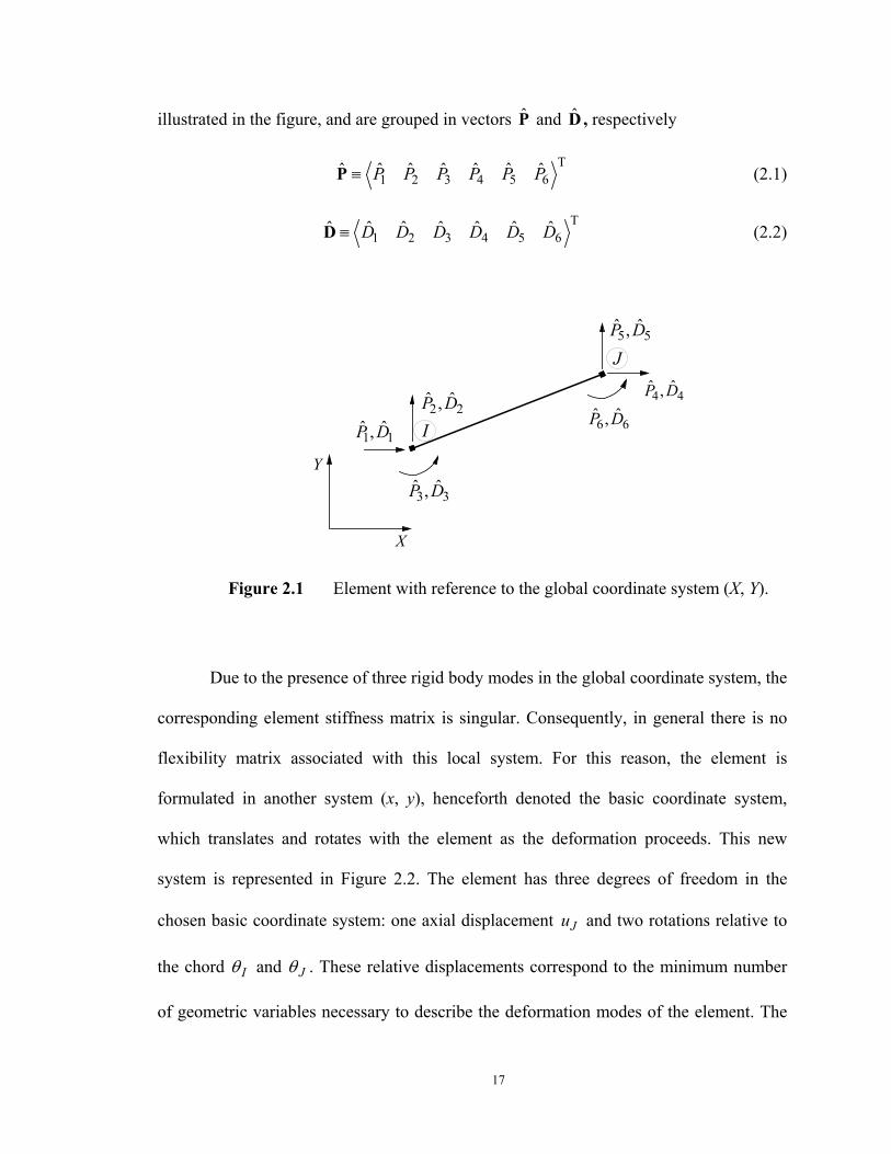
17

illustrated in the figure, and are grouped in vectors P and D , respectively

T1 2 3 4 5 6

ˆ ˆ ˆ ˆ ˆ ˆ ˆP P P P P P≡P (2.1)

T1 2 3 4 5 6

ˆ ˆ ˆ ˆ ˆ ˆ ˆD D D D D D≡D (2.2)

2 2ˆ ˆ,P D

X

Y

1 1ˆ ˆ,P D

3 3ˆ ˆ,P D

5 5ˆ ˆ,P D

4 4ˆ ˆ,P D

6 6ˆ ˆ,P D

I

J

Figure 2.1 Element with reference to the global coordinate system (X, Y).

Due to the presence of three rigid body modes in the global coordinate system, the

corresponding element stiffness matrix is singular. Consequently, in general there is no

flexibility matrix associated with this local system. For this reason, the element is

formulated in another system (x, y), henceforth denoted the basic coordinate system,

which translates and rotates with the element as the deformation proceeds. This new

system is represented in Figure 2.2. The element has three degrees of freedom in the

chosen basic coordinate system: one axial displacement Ju and two rotations relative to

the chord Iθ and Jθ . These relative displacements correspond to the minimum number

of geometric variables necessary to describe the deformation modes of the element. The

18

three statically independent end forces related to these displacements are one axial force

P and two bending moments IM and JM . These element forces and displacements are

grouped in vectors P and D respectively

1

2

3

J

I

J

P uPP

θθ

≡ =

P (2.3)

1

2

3

J

I

J

D uDD

θθ

≡ =

D (2.4)

3 3,P D

1 1,P D

2 2,P D

x

y

deformed configuration

undeformed configuration

basic coordinate system

2 2ˆ ˆ,P D

X

Y

1 1ˆ ˆ,P D

3 3ˆ ˆ,P D

5 5ˆ ˆ,P D

J

I

6 6ˆ ˆ,P D

4 4ˆ ˆ,P D

I

J

Figure 2.2 Global and basic coordinate systems.

Approximate transformations between the two systems of coordinates (x, y) and

(X, Y), which are only valid for small rotations, have been used in other works based on

19

the flexibility formulation, such as Carol and Murcia (1989), and Neuenhofer and

Filippou (1998). In order to handle arbitrarily large rotations, exact expressions for the

transformation of force and displacements between these two coordinate systems must be

employed. For this purpose, the present work adopts the idea of the corotational

formulation, which will be discussed in section 2.9.

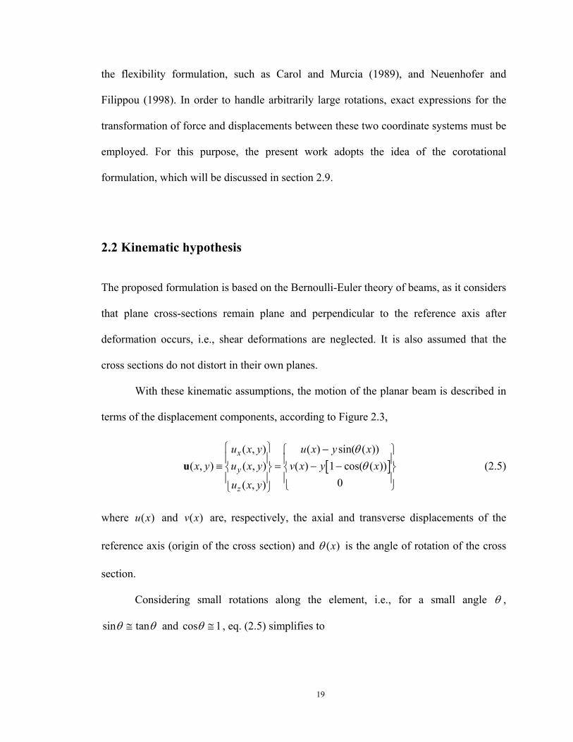
2.2 Kinematic hypothesis

The proposed formulation is based on the Bernoulli-Euler theory of beams, as it considers

that plane cross-sections remain plane and perpendicular to the reference axis after

deformation occurs, i.e., shear deformations are neglected. It is also assumed that the

cross sections do not distort in their own planes.

With these kinematic assumptions, the motion of the planar beam is described in

terms of the displacement components, according to Figure 2.3,

[ ]( , ) ( ) sin( ( ))

( , ) ( , ) ( ) 1 cos( ( ))0( , )

x

y

z

u x y u x y xx y u x y v x y x

u x y

θθ

− ≡ = − −

u (2.5)

where ( )u x and ( )v x are, respectively, the axial and transverse displacements of the

reference axis (origin of the cross section) and ( )xθ is the angle of rotation of the cross

section.

Considering small rotations along the element, i.e., for a small angle θ ,

sin tanθ θ≅ and cos 1θ ≅ , eq. (2.5) simplifies to

20

d ( )( , ) ( ) tan( ( )) ( )d

( , ) ( , ) ( ) ( )0( , ) 0

x

y

z

v xu x y u x y x u x yx

x y u x y v x v xu x y

θ − − ≡ ≅ =

u (2.6)

Neglecting shear and in-plane distortion of the section, the only non-zero

component of the Green-Lagrange strain tensor at the reference axis is

221 12 2

yx xxx

uu uEx x x

∂ ∂ ∂ = + + ∂ ∂ ∂ (2.7)

y v,

x u,

( )u x

( )v x

y

y θ

siny θ

cosy θ

cross section

Figure 2.3 Displacement field of the beam.

Assuming that the term xu x∂ ∂ is small compared to unity, the term ( )212 xu x∂ ∂

is negligible compared to xu x∂ ∂ . This assumption is also used in the von Kármán

theory of thin elastic plates, where the membrane part of the strain-displacement

relationships for moderately large deformation analysis has a similar form (Timoshenko

and Woinowsky-Krieger (1959)). According to Crisfield (1991), for approximate

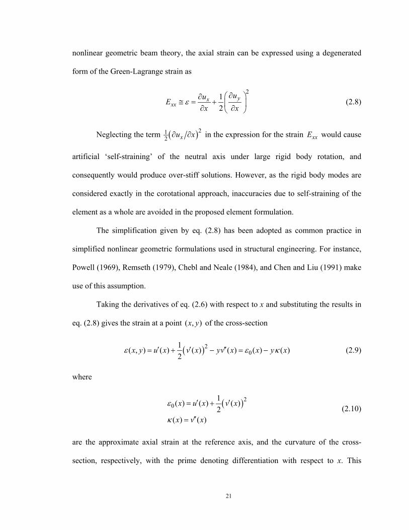
21

nonlinear geometric beam theory, the axial strain can be expressed using a degenerated

form of the Green-Lagrange strain as

212

yxxx

uuEx x

ε∂ ∂

≅ = + ∂ ∂ (2.8)

Neglecting the term ( )212 xu x∂ ∂ in the expression for the strain xxE would cause

artificial ‘self-straining’ of the neutral axis under large rigid body rotation, and

consequently would produce over-stiff solutions. However, as the rigid body modes are

considered exactly in the corotational approach, inaccuracies due to self-straining of the

element as a whole are avoided in the proposed element formulation.

The simplification given by eq. (2.8) has been adopted as common practice in

simplified nonlinear geometric formulations used in structural engineering. For instance,

Powell (1969), Remseth (1979), Chebl and Neale (1984), and Chen and Liu (1991) make

use of this assumption.

Taking the derivatives of eq. (2.6) with respect to x and substituting the results in

eq. (2.8) gives the strain at a point ( , )x y of the cross-section

( )2 01( , ) ( ) ( ) ( ) ( ) ( )2

x y u x v x yv x x y xε ε κ′ ′ ′′= + − = − (2.9)

where

( )201( ) ( ) ( )2

( ) ( )

x u x v x

x v x

ε

κ

′ ′= +

′′=(2.10)

are the approximate axial strain at the reference axis, and the curvature of the cross-

section, respectively, with the prime denoting differentiation with respect to x. This

22

reference axis does not necessarily pass through the geometric centroid of the cross

sections.

The term ( )( )21 2 ( )v x′ introduces the geometric nonlinearity in the compatibility

(strain-displacement) relation, but this relation is still approximate as higher order terms

are neglected. Therefore, the target problems of this formulation are structures subject to

moderately large deformations within each element (as opposed to finite deformation

problems).

Eq. (2.9) can be rewritten in matrix form as

( , ) ( ) ( )x y y xε = a d (2.11)

where

T0( ) ( ) ( )x x xε κ=d (2.12)

are henceforth denoted generalized section strains (or section deformations), and

( ) 1y y= −a (2.13)

is a row matrix that relates the generalized section strains with the strain at a point of the

cross-section.

2.3 Variational formulation

The element formulation can be derived from the Hellinger-Reissner potential, a two-

field functional of displacements and stresses. For the case at hand, where only the axial

stress in the direction x is non-zero, the displacement field is given by eq. (2.6) and the

compatibility relation is given by eq. (2.8).

23

In order to define the Hellinger-Reissner functional, the following assumptions

are necessary: a) Conservative external loads (body forces and boundary tractions);

b) Hyperelastic material behavior.

The external loads are conservative if there exists a functional (body forces are

omitted for simplicity’s sake) such that

Text ( ) d

tΓ

Π = − Γ∫u t u (2.14)

where t are the imposed tractions on the part tΓ of the element boundary Γ . This

functional is referred to as the potential energy of the external loading. A common

example of conservative loads are ‘dead’ loads (with constant directions).

A material model is hyperelastic (or Green elastic) if there exists a stored energy

function ( )W ε , such that the axial stress σ can be expressed as a function of strain ε as

( )W εσε

∂=

∂(2.15)

If this constitutive relation has a unique inverse, i.e., if ( )W ε is strictly convex, a

unique strain ε can be found for a given stress, using the complementary energy density

( )( ) ( ) ( )Wχ σ σε σ ε σ= − (2.16)

Taking the derivative of eq. (2.16) with respect to σ gives

( )( )( ) ( ) ( )( )

( ) ( )( )

( )

W ε σχ σ ε σ ε σε σ σσ σ ε σ

ε σ ε σε σ σ σσ σ

ε σ

∂∂ ∂ ∂= + −

∂ ∂ ∂ ∂∂ ∂

= + −∂ ∂

=

(2.17)

Although this inverse form is possible for most elastic material models in the

24

range of small strains, this is not always the case for large elastic strains.

With these assumptions, the following form of the Hellinger-Reissner functional,

considering the degenerated form of the Green-Lagrange strain given in eq. (2.8), can be

stated as

2

ext1( , ) ( ) d ( )2

yxHR

uux x

σ σ χ σΩ

∂ ∂ Π = + − Ω +Π ∂ ∂ ∫u u (2.18)

where Ω is the undeformed volume of the element.

In the following derivations, for the sake of brevity, often the same symbol will be

used for a function written in terms of different (but related) arguments. For instance,

( ) ( ( ))χ χ σ≡S S , with S being the stress resultant vector, defined below, will still

represent the complementary energy density ( )χ σ , as an abuse of notation.

Performing the integration over the area A of the cross-sections, and using the

displacements at the reference axis

0( )

( ) ( ,0)( )

u xx x

v x

≡ =

u u (2.19)

eq. (2.18) can be rewritten for stress resultants in matrix form as

2T T

0

1( , ) ( ) d2HR

L

u vx

vχ

′ ′+ Π = − − ′′ ∫S u S S P D (2.20)

where L is the undeformed element length, and

TT Td d d

A A A

N M A y A Aσ σ σ= = − =∫ ∫ ∫S a (2.21)

is the stress resultant vector, with N being the axial force and M the bending moment at a

25

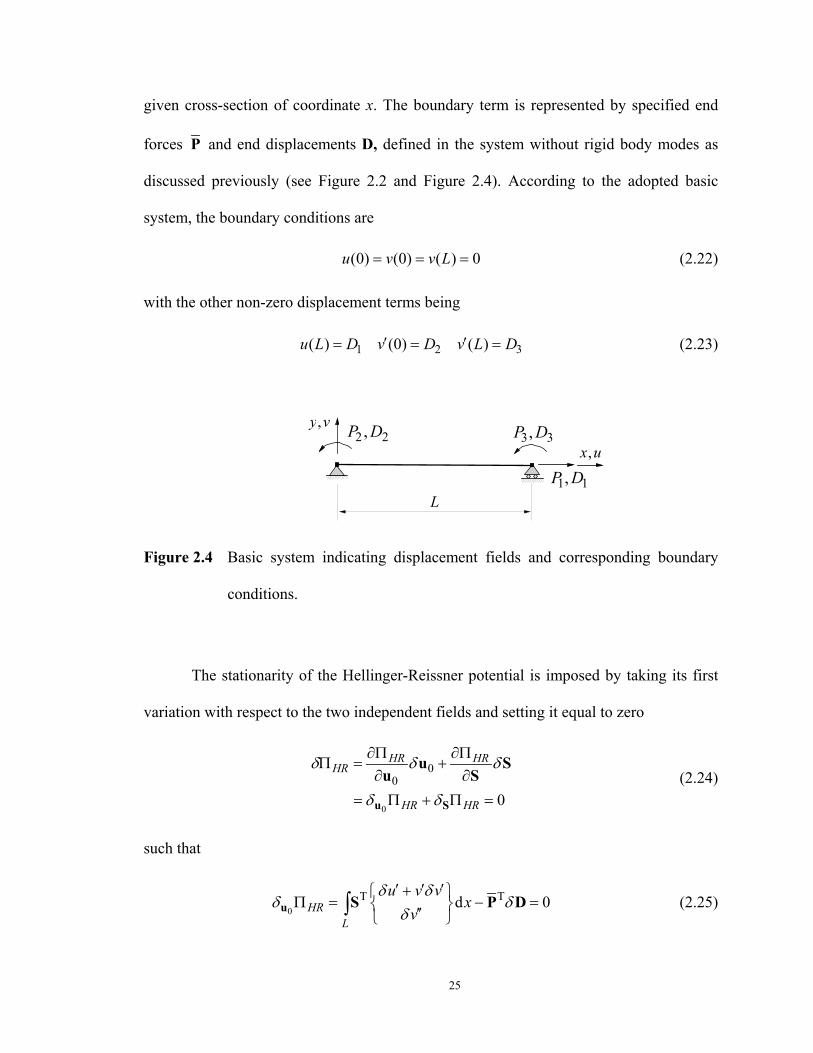
given cross-section of coordinate x. The boundary term is represented by specified end

forces P and end displacements D, defined in the system without rigid body modes as

discussed previously (see Figure 2.2 and Figure 2.4). According to the adopted basic

system, the boundary conditions are

(0) (0) ( ) 0u v v L= = = (2.22)

with the other non-zero displacement terms being

1 2 3( ) (0) ( )u L D v D v L D′ ′= = = (2.23)

y v,

x u,

1 1,P D

3 3,P D2 2,P D

L

Figure 2.4 Basic system indicating displacement fields and corresponding boundary

conditions.

The stationarity of the Hellinger-Reissner potential is imposed by taking its first

variation with respect to the two independent fields and setting it equal to zero

0

00

0

HR HRHR

HR HR

δ δ δ

δ δ

∂Π ∂ΠΠ = +

∂ ∂= Π + Π =u S

u Su S (2.24)

such that

0T Td 0HR

L

u v vx

vδ δ

δ δδ′ ′ ′+

Π = − = ′′ ∫u S P D (2.25)

26

and

21( ) d 02T

HRL

u vx

v

χδ δ ′ ′+ ∂ Π = − = ∂ ′′

∫SSS

S(2.26)

Eq. (2.25) can be identified as the Principle of Virtual Work, i.e., the weak form

of the equilibrium equations.

From the definition of the complementary energy density, the second term in

square brackets in eq. (2.26) corresponds to the section deformations (eq.(2.12)), i.e., the

work conjugate of the stress resultants S

( )χ∂=

∂Sd

S(2.27)

Therefore, substitution of eq. (2.27) into eq. (2.26) gives

2T

1d 02

L

u vx

vδ

′ ′+ − = ′′ ∫ S d (2.28)

Consequently, eq. (2.28) corresponds to the weak statement of the compatibility

(strain-displacement) relation (2.10). For the particular case of linear geometry, i.e., if the

quadratic term 2(1/ 2)v′ is neglected, eq. (2.28) leads to the Principle of Complementary

Virtual Work (or Principle of Virtual Forces, as commonly called in linear structural

analysis).

Although the Helinger-Reissner functional is based on the assumptions of a

hyperelastic material model and conservative external loading, the weak form of the

equilibrium equation (obtained from eq. (2.25)) and the weak form of the compatibility

equation (obtained from eq. (2.28)) are also valid for structures with other types of

27

material.

Therefore, it is less restrictive to use the weak form of the compatibility equation

as the basis of the proposed formulation. However, there is an advantage in deriving the

present formulation from a variational principle: it allows the concentration of all

intrinsic characteristics of the problem in a single expression.

Based on this, it should be clear that the proposed element formulation can be used

to solve more general problems such as, for instance, elasto-plastic analysis. Some

examples of this more general case will be presented to validate the extension of the

formulation to this type of material.

2.4 Equilibrium equations

The equations of equilibrium, consistent with the kinematic hypothesis stated in

Section 2.2, are obtained from eq. (2.25), which is rewritten here in expanded form

[ ] 1 1 2 2 3 3( ) d 0L

N u v v M v x P D P D P Dδ δ δ δ δ δ′ ′ ′ ′′+ + − − − =∫ (2.29)

It should be noted that the bar over the forces P, which indicate that those are

specified quantities, are omitted for brevity of notation. However, no confusion should

occur.

This equation is valid for all kinematically admissible uδ and vδ satisfying the

essential boundary conditions (see Figure 2.4)

(0) (0) ( ) 0u v v Lδ δ δ= = = (2.30)

Integration of eq. (2.29) by parts and application of the boundary conditions

28

(2.30) lead to

[ ] [ ] [ ] [ ]

0

1 1 2 2 3 3

( ) d

( ) (0) ( ) 0

LN u Nv M v x

N L P D M P D M L P D

δ δ

δ δ δ

′ ′ ′ ′′+ − +

− + + + + − + =

∫ (2.31)

If eq. (2.31) is to be satisfied for all admissible variations, the following equations

of equilibrium (consistent forms of linear and angular momentum balance equations) are

obtained

2

2

( ) 0

( ) ( )( ) 0

dN xdx

d M x d dv xN xdx dxdx

=

− + =

in [0, ]L (2.32)

with the following natural boundary conditions

1 2 3( ) (0) ( )N L P M P M L P= = − = (2.33)

Since the displacement variation fields are arbitrary in this derivation (i.e., a

displacement interpolation function was not adopted), the equilibrium equations are

satisfied pointwise (strong form). This is in contrast to stiffness based formulations,

which satisfy the equilibrium equations in the average sence (weak form).

From eqs. (2.32) it is observed that the axial force ( )N x is constant along the

element. The expression for the bending moment ( )M x is obtained by integrating the

second of eqs. (2.32) twice. Then, considering the natural boundary conditions (2.33), the

following stress resultant fields are obtained:

1

1 2 3

( )

( ) ( ) 1

N x Px xM x v x P P PL L

=

= + − +

(2.34)

This equation can be rewritten in matrix form as a relation between section forces

29

( )xS and end forces P

( ) ( )x x=S b P (2.35)

where

1 0 0( ) ,

( ) 1xx

v Lξ

ξ ξ ξ

= = − b (2.36)

is denoted the matrix of displacement-dependent force interpolation functions, with

x Lξ = being the natural coordinate along the element.

This relation between section forces ( )xS and end forces P can also be obtained

directly considering that equilibrium is satisfied in the deformed configuration. However,

if equilibrium is to be imposed directly, usually physical interpretation of the quantities

involved are necessary, which is not always straightforward. In addition, the present

derivation shows that the expressions used for the section forces (eq. (2.35)) are

consistent with the adopted kinematic assumptions. This fact is not observed in Carol and

Murcia (1989), where the forces are interpolated according to eq. (2.36), but a linear

strain-displacement relation is used, i.e., the term ( )212 yu x∂ ∂ in eq. (2.8) is neglected.

2.5 Weak form of the compatibility equation

The compatibility equations are imposed weakly using eq. (2.28), which is repeated here

in expanded form

( )20

1 d 02L

N u v M v xδ ε δ κ ′ ′ ′′+ − + − = ∫ (2.37)

30

If this equation could be satisfied for all statically admissible variations Nδ and

Mδ (i.e., all virtual force systems in equilibrium), it would imply the strong form of the

compatibility relations (2.10). However, for a reduced set of admissible variations Nδ

and Mδ , the compatibility relations are satisfied only in the average sense. The subset of

these admissible variations used in the present element formulation is determined as

follows.

Integration of eq. (2.37) by parts and consideration of the boundary conditions

(2.22) lead to

0

1 2 3

1 ( ) d2

( ) (0) ( ) 0L

N u Nv M v N M x

N L D M D M L D

δ δ δ δ ε δ κ

δ δ δ

′ ′ ′ ′′+ − + +

− + − =

∫ (2.38)

In order to enforce a stationary point of the Helinger-Reissner potential, the first

two terms of this equation are set equal to zero for given displacements u and v, yielding

the following relation between the variations Nδ and Mδ

2

2

( ) 0

( ) 1 ( )( ) 02

d N xdx

d M x d dv xN xdx dxdx

δ

δ δ

=

− + =

in [0, ]L (2.39)

The similarity between eqs. (2.39) and (2.32) should be noted. Accordingly, from

eqs. (2.39) it is observed that the virtual axial force ( )N xδ is constant along the element.

Again, the expression for the virtual bending moment ( )M xδ is obtained integrating the

second of the eqs. (2.39), twice. Hence, the following virtual fields are obtained:

1

1 2 3

( )( ) 1 ( ) 1( )

2

PN x

x x xv x P P PM xL L

δδ

δδ δ δδ

≡ = + − +

S (2.40)

31

This equation can be rewritten in matrix form as a relation between virtual section

forces ( )xδS and virtual end forces δP

*( ) ( )x xδ δ=S b P (2.41)

where

*1 0 0

( ) ,1 ( ) 12

xxLv

ξξ ξ ξ

= = −

b (2.42)

Considering the virtual forces given by eq. (2.40), eq. (2.38) can be expressed in

matrix form as

TT( ) ( )dL

x x xδ δ=∫ S d P D (2.43)

Substitution of eq. (2.41) into eq. (2.43) implies

T * T T( ) ( )dL

x x xδ δ=∫P b d P D (2.44)

For arbitrary virtual end forces (variations) δP , eq. (2.44) leads to

* T( ) ( )dL

x x x= ∫D b d (2.45)

which allows for the determination of the element end displacements in terms of the

section deformations along the element.

2.6 Section constitutive relations

The use of a constitutive relation based on the complementary energy density as in

32

eq. (2.27) is not always possible as discussed before.

Therefore, other nonlinear material constitutive relationships are used with the

proposed element. For path dependent material models, the only additional complexity

lies in the computational implementation of the state determination procedure.

The nonlinear relation between section forces ( )xS and section deformations

( )xd , i.e., the section constitutive relation, can be determined by integration of the stress-

strain relation over the sections, usually applying a numerical integration procedure.

Substitution of eq. (2.11) into eq. (2.21) results in the nonlinear section

constitutive relation

( ) ( )T T( ) ( ) ( , ) d ( ) ( ) ( ) dA A

x y x y A y y x Aσ ε σ= =∫ ∫S a a a d (2.46)

which can be expressed in terms of section deformations, in more general form, as

[ ]( ) ( )x x=S C d (2.47)

where [ ]( )xC d represents a general function that permits the computation of section

forces for given section deformations. The linearization of the section constitutive

relation (2.46) is obtained using the tangent section stiffness matrix

( ) ( ) T

T T

( ) ( , )( ) ( ) d( ) ( )

( , ) ( , )( ) d ( ) ( , ) ( )d( , ) ( )

A

tA A

x x yx y Ax x

x y x yy A y E x y y Ax y x

∂ σ∂

σ εε

∂= =

∂

∂ ∂= =

∂ ∂

∫

∫ ∫

C dk d a

d d

a a ad

(2.48)

where

( , )( , )( , )t

x yE x yx y

σε

∂=∂

(2.49)

33

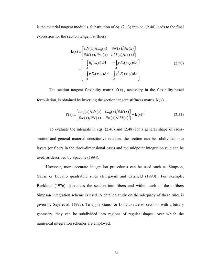
is the material tangent modulus. Substitution of eq. (2.13) into eq. (2.48) leads to the final

expression for the section tangent stiffness

0

0

2

( ) ( ) ( ) ( )( )

( ) ( ) ( ) ( )

( , )d ( , )d

=( , )d ( , )d

t tA A

t tA A

N x x N x xx

M x x M x x

E x y A y E x y A

y E x y A y E x y A

ε κε κ

∂ ∂ ∂ ∂ ≡ ∂ ∂ ∂ ∂ − −

∫ ∫

∫ ∫

k

(2.50)

The section tangent flexibility matrix ( )xf , necessary in the flexibility-based

formulation, is obtained by inverting the section tangent stiffness matrix ( )xk .

0 0 -1( ) ( ) ( ) ( )( ) ( )

( ) ( ) ( ) ( )x N x x M x

x xx N x x M x

ε εκ κ

∂ ∂ ∂ ∂ ≡ = ∂ ∂ ∂ ∂

f k (2.51)

To evaluate the integrals in eqs. (2.46) and (2.48) for a general shape of cross-

section and general material constitutive relation, the section can be subdivided into

layers (or fibers in the three-dimensional case) and the midpoint integration rule can be

used, as described by Spacone (1994).

However, more accurate integration procedures can be used such as Simpson,

Gauss or Lobatto quadrature rules (Burgoyne and Crisfield (1990)). For example,

Backlund (1976) discretizes the section into fibers and within each of these fibers

Simpson integration scheme is used. A detailed study on the adequacy of these rules is

given by Saje et al. (1997). To apply Gauss or Lobatto rule to sections with arbitrary

geometry, they can be subdivided into regions of regular shapes, over which the

numerical integration schemes are employed.

34

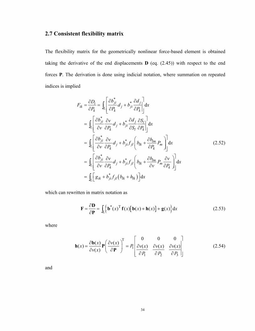
2.7 Consistent flexibility matrix

The flexibility matrix for the geometrically nonlinear force-based element is obtained

taking the derivative of the end displacements D (eq. (2.45)) with respect to the end

forces P. The derivation is done using indicial notation, where summation on repeated

indices is implied

**

**

**

**

d

d

d

d

ji jiik j jiLk k k

ji j lj jiL k l k

ji lmj ji jl lk mL k k

ji lmj ji jl lk mL k k

b dDF d b xP P P

b dv Sd b xv P S P

b v bd b f b P xv P P

b v b vd b f b P xv P v P

∂ ∂∂ = = +

∂ ∂ ∂ ∂ ∂∂ ∂ = +∂ ∂ ∂ ∂

∂ ∂ ∂ = + + ∂ ∂ ∂ ∂ ∂ ∂ ∂ = + + ∂ ∂ ∂ ∂

∫

∫

∫

∫

( )* dik ji jl lk lkLg b f b h x = + + ∫

(2.52)

which can rewritten in matrix notation as

[ ] * T( ) ( ) ( ) ( ) ( ) dL

x x x x x x∂= = + +∂ ∫DF b f b h gP

(2.53)

where

T

1

1 2 3

0 0 0( ) ( )( ) ( ) ( ) ( )( )x v xx P v x v x v x

v xP P P

∂ ∂ = = ∂ ∂ ∂ ∂ ∂ ∂ ∂ ∂

bh PP

(2.54)

and

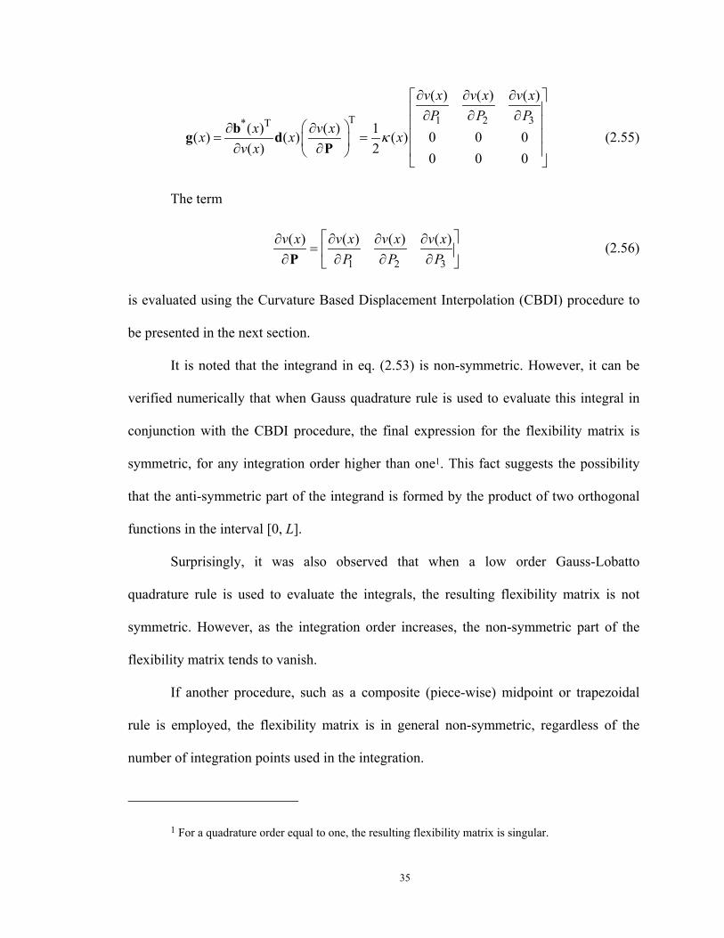
35

T 1 2 3* T

( ) ( ) ( )

( ) ( ) 1( ) ( ) ( ) 0 0 0( ) 2

0 0 0

v x v x v xP P P

x v xx x xv x

κ

∂ ∂ ∂ ∂ ∂ ∂ ∂ ∂ = = ∂ ∂

bg dP

(2.55)

The term

1 2 3

( ) ( ) ( ) ( )v x v x v x v xP P P

∂ ∂ ∂ ∂= ∂ ∂ ∂ ∂ P

(2.56)

is evaluated using the Curvature Based Displacement Interpolation (CBDI) procedure to

be presented in the next section.

It is noted that the integrand in eq. (2.53) is non-symmetric. However, it can be

verified numerically that when Gauss quadrature rule is used to evaluate this integral in

conjunction with the CBDI procedure, the final expression for the flexibility matrix is

symmetric, for any integration order higher than one1. This fact suggests the possibility

that the anti-symmetric part of the integrand is formed by the product of two orthogonal

functions in the interval [0, L].

Surprisingly, it was also observed that when a low order Gauss-Lobatto

quadrature rule is used to evaluate the integrals, the resulting flexibility matrix is not

symmetric. However, as the integration order increases, the non-symmetric part of the

flexibility matrix tends to vanish.

If another procedure, such as a composite (piece-wise) midpoint or trapezoidal

rule is employed, the flexibility matrix is in general non-symmetric, regardless of the

number of integration points used in the integration.

1 For a quadrature order equal to one, the resulting flexibility matrix is singular.

36

These observations suggest the possibility that the symmetric characteristic of the

flexibility matrix is affected by the way the displacements are interpolated from the

curvatures using the CBDI procedure. This possible explanation is further discussed in

the next section, after the CBDI procedure is presented.

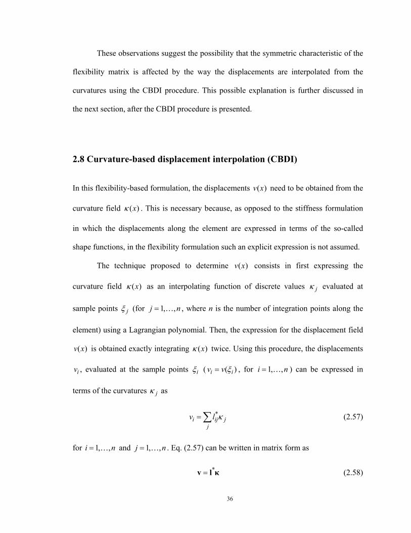
2.8 Curvature-based displacement interpolation (CBDI)

In this flexibility-based formulation, the displacements ( )v x need to be obtained from the

curvature field ( )xκ . This is necessary because, as opposed to the stiffness formulation

in which the displacements along the element are expressed in terms of the so-called

shape functions, in the flexibility formulation such an explicit expression is not assumed.

The technique proposed to determine ( )v x consists in first expressing the

curvature field ( )xκ as an interpolating function of discrete values jκ evaluated at

sample points jξ (for 1, ,j n= … , where n is the number of integration points along the

element) using a Lagrangian polynomial. Then, the expression for the displacement field

( )v x is obtained exactly integrating ( )xκ twice. Using this procedure, the displacements

iv , evaluated at the sample points iξ ( ( )i iv v ξ= , for 1, ,i n= … ) can be expressed in

terms of the curvatures jκ as

*i ij j

jv l κ=∑ (2.57)

for 1, ,i n= … and 1, ,j n= … . Eq. (2.57) can be written in matrix form as

*=v l κ (2.58)

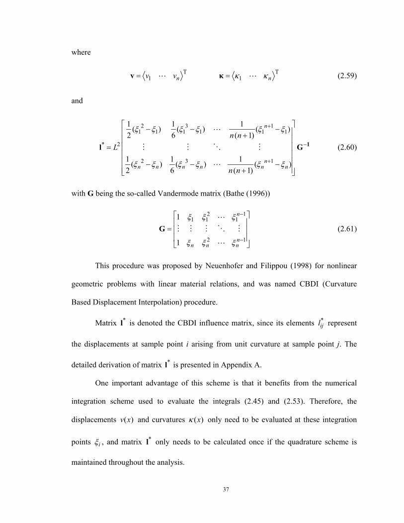
37

where

T1 nv v=v T

1 nκ κ=κ (2.59)

and

2 3 11 1 1 1 1 1

* 2

2 3 1

1 1 1( ) ( ) ( )2 6 ( 1)

1 1 1( ) ( ) ( )2 6 ( 1)

n

nn n n n n n

n nL

n n

ξ ξ ξ ξ ξ ξ

ξ ξ ξ ξ ξ ξ

+

−

+

− − − + =

− − − +

1l G (2.60)

with G being the so-called Vandermode matrix (Bathe (1996))

2 11 1 1

2 1

1

1

n

nn n n

ξ ξ ξ

ξ ξ ξ

−

−

=

G (2.61)

This procedure was proposed by Neuenhofer and Filippou (1998) for nonlinear

geometric problems with linear material relations, and was named CBDI (Curvature

Based Displacement Interpolation) procedure.

Matrix *l is denoted the CBDI influence matrix, since its elements *ijl represent

the displacements at sample point i arising from unit curvature at sample point j. The

detailed derivation of matrix *l is presented in Appendix A.

One important advantage of this scheme is that it benefits from the numerical

integration scheme used to evaluate the integrals (2.45) and (2.53). Therefore, the

displacements ( )v x and curvatures ( )xκ only need to be evaluated at these integration

points iξ , and matrix *l only needs to be calculated once if the quadrature scheme is

maintained throughout the analysis.

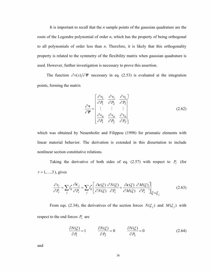
38

It is important to recall that the n sample points of the gaussian quadrature are the

roots of the Legendre polynomial of order n, which has the property of being orthogonal

to all polynomials of order less than n. Therefore, it is likely that this orthogonality

property is related to the symmetry of the flexibility matrix when gaussian quadrature is

used. However, further investigation is necessary to prove this assertion.

The function ( )v x∂ ∂ P necessary in eq. (2.53) is evaluated at the integration

points, forming the matrix

1 1 1

1 2 3

1 2 3

n n n

v v vP P P

v v vP P P

∂ ∂ ∂∂ ∂ ∂

∂∂

∂ ∂ ∂∂ ∂ ∂

=

vP

(2.62)

which was obtained by Neuenhofer and Filippou (1998) for prismatic elements with

linear material behavior. The derivation is extended in this dissertation to include

nonlinear section constitutive relations.

Taking the derivative of both sides of eq. (2.57) with respect to rP (for

1, ,3r = … ), gives

* * ( ) ( ) ( ) ( )( ) ( )

j

jiij ij

r r r rj j

v N Ml lP P N P M P

∂κ∂ ∂κ ξ ∂ ξ ∂κ ξ ∂ ξ∂ ∂ ∂ ξ ∂ ∂ ξ ∂ ξ ξ

= = +

=∑ ∑ (2.63)

From eqs. (2.34), the derivatives of the section forces ( )jN ξ and ( )jM ξ with

respect to the end forces rP are

1 2 3

( ) ( ) ( )1 0 0N N NP P Pξ ξ ξ∂ ∂ ∂

= = =∂ ∂ ∂

(2.64)

and

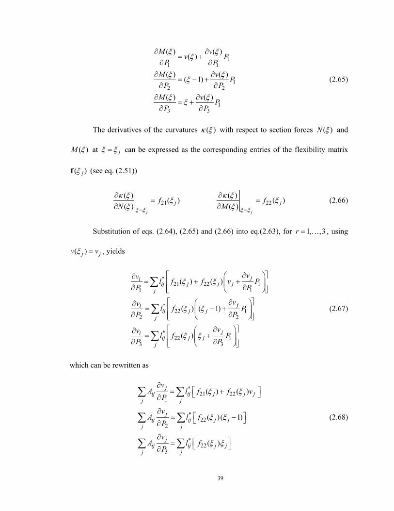
39

11 1

12 2

13 3

( ) ( )( )

( ) ( )( 1)

( ) ( )

M vv PP P

M v PP P

M v PP P

ξ ξξ

ξ ξξ

ξ ξξ

∂ ∂= +

∂ ∂∂ ∂

= − +∂ ∂

∂ ∂= +

∂ ∂

(2.65)

The derivatives of the curvatures ( )κ ξ with respect to section forces ( )N ξ and

( )M ξ at jξ ξ= can be expressed as the corresponding entries of the flexibility matrix

( )jξf (see eq. (2.51))

21( ) ( )( )

j

jfN ξ ξ

κ ξ ξξ =

∂=

∂ 22

( ) ( )( )

j

jfM ξ ξ

κ ξ ξξ =

∂=

∂(2.66)

Substitution of eqs. (2.64), (2.65) and (2.66) into eq.(2.63), for 1, ,3r = … , using

( )j jv vξ = , yields

*21 22 1

1 1

*22 1

2 2

*22 1

3 3

( ) ( )

( ) ( 1)

( )

jiij j j j

j

jiij j j

j

jiij j j

j

vv l f f v PP P

vv l f PP P

vv l f PP P

ξ ξ

ξ ξ

ξ ξ

∂ ∂= + + ∂ ∂

∂ ∂= − + ∂ ∂

∂ ∂= + ∂ ∂

∑

∑

∑

(2.67)

which can be rewritten as

*21 22

1

*22

2

*22

3

( ) ( )

( ) ( 1)

( )

jij ij j j j

j j

jij ij j j

j j

jij ij j j

j j

vA l f f v

P

vA l f

P

vA l f

P

ξ ξ

ξ ξ

ξ ξ

∂ = + ∂

∂ = − ∂

∂ = ∂

∑ ∑

∑ ∑

∑ ∑

(2.68)

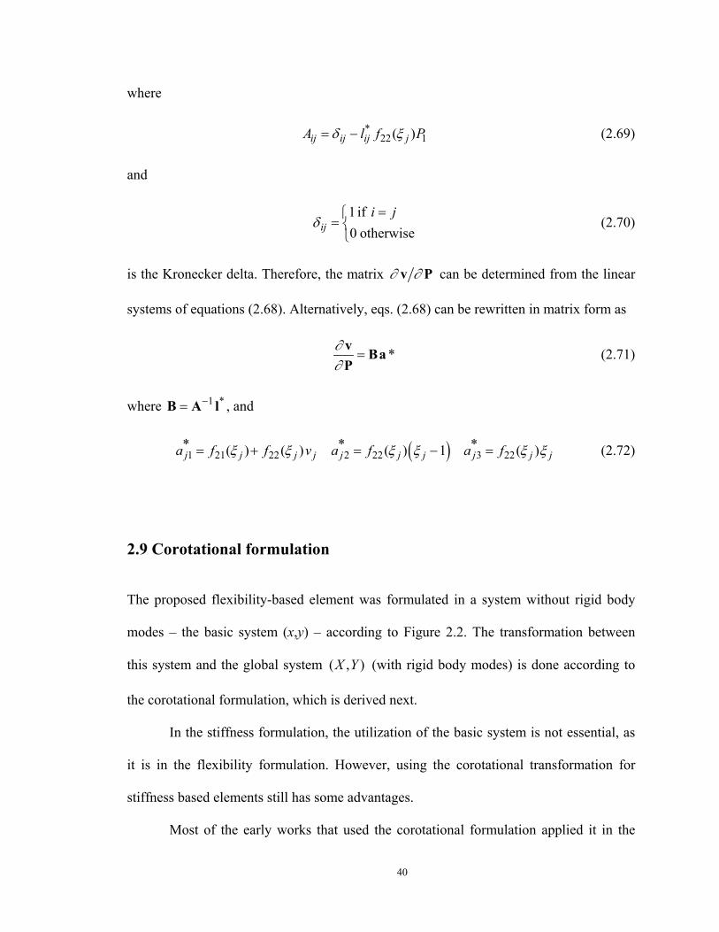
40

where

*22 1( )ij ij ij jA l f Pδ ξ= − (2.69)

and

1 if0 otherwiseij

i jδ

==

(2.70)

is the Kronecker delta. Therefore, the matrix ∂ ∂v P can be determined from the linear

systems of equations (2.68). Alternatively, eqs. (2.68) can be rewritten in matrix form as

*∂∂

=v BaP

(2.71)

where 1 *−=B A l , and

( )1 21 22 2 22 3 22* * *( ) ( ) ( ) 1 ( )j j j j j j j j j ja f f v a f a fξ ξ ξ ξ ξ ξ= + = − = (2.72)

2.9 Corotational formulation

The proposed flexibility-based element was formulated in a system without rigid body

modes – the basic system (x,y) – according to Figure 2.2. The transformation between

this system and the global system ( , )X Y (with rigid body modes) is done according to

the corotational formulation, which is derived next.

In the stiffness formulation, the utilization of the basic system is not essential, as

it is in the flexibility formulation. However, using the corotational transformation for

stiffness based elements still has some advantages.

Most of the early works that used the corotational formulation applied it in the

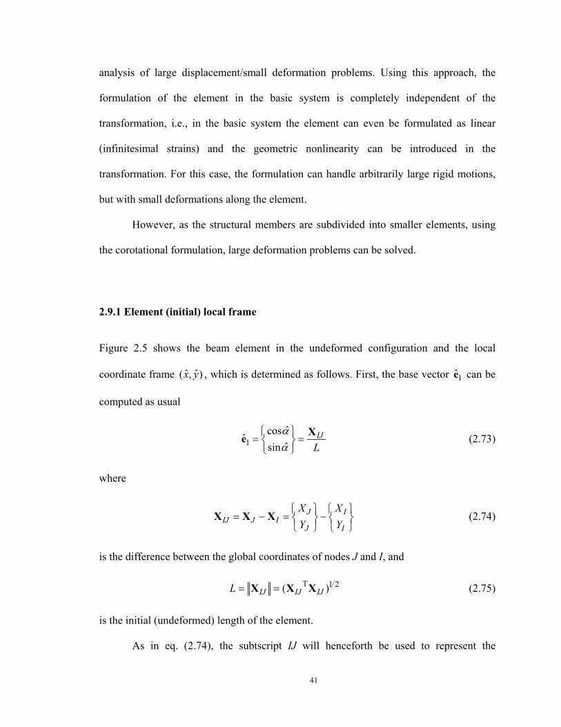
41

analysis of large displacement/small deformation problems. Using this approach, the

formulation of the element in the basic system is completely independent of the

transformation, i.e., in the basic system the element can even be formulated as linear

(infinitesimal strains) and the geometric nonlinearity can be introduced in the

transformation. For this case, the formulation can handle arbitrarily large rigid motions,

but with small deformations along the element.

However, as the structural members are subdivided into smaller elements, using

the corotational formulation, large deformation problems can be solved.

2.9.1 Element (initial) local frame

Figure 2.5 shows the beam element in the undeformed configuration and the local

coordinate frame ˆ ˆ( , )x y , which is determined as follows. First, the base vector 1e can be

computed as usual

1ˆcos

ˆˆsin

IJL

αα

= =

Xe (2.73)

where

J IIJ J I

J I

X XY Y

= − = −

X X X (2.74)

is the difference between the global coordinates of nodes J and I, and

T 1 2( )IJ IJ IJL = =X X X (2.75)

is the initial (undeformed) length of the element.

As in eq. (2.74), the subtscript IJ will henceforth be used to represent the

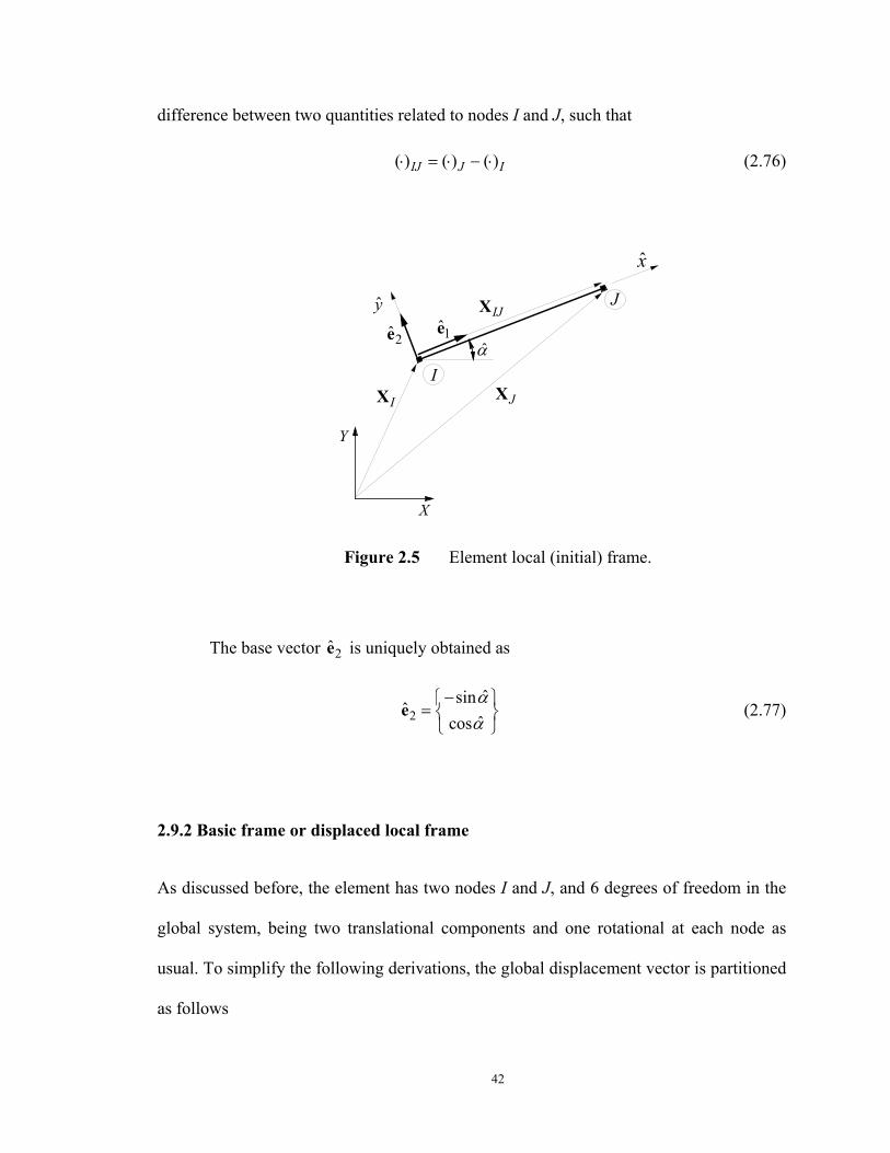
42

difference between two quantities related to nodes I and J, such that

( ) ( ) ( )IJ J I⋅ = ⋅ − ⋅ (2.76)

IJX

X

Y

x

J

IIX JX

y

2e 1eα

Figure 2.5 Element local (initial) frame.

The base vector 2e is uniquely obtained as

2ˆsin

ˆˆcosαα

− =

e (2.77)

2.9.2 Basic frame or displaced local frame

As discussed before, the element has two nodes I and J, and 6 degrees of freedom in the

global system, being two translational components and one rotational at each node as

usual. To simplify the following derivations, the global displacement vector is partitioned

as follows

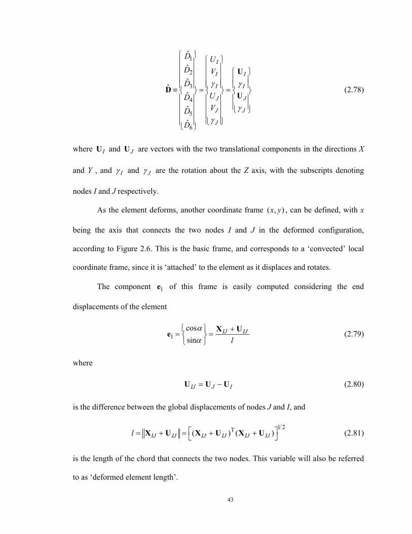
43

1

2

3

4

5

6

ˆ

ˆ

ˆˆ

ˆ

ˆ

ˆ

I

I I

I I

J J

J J

J

D UD VD

UDVD

D

γ γ

γγ

≡ = =

U

DU

(2.78)

where IU and JU are vectors with the two translational components in the directions X

and Y , and Iγ and Jγ are the rotation about the Z axis, with the subscripts denoting

nodes I and J respectively.

As the element deforms, another coordinate frame ( , )x y , can be defined, with x

being the axis that connects the two nodes I and J in the deformed configuration,

according to Figure 2.6. This is the basic frame, and corresponds to a ‘convected’ local

coordinate frame, since it is ‘attached’ to the element as it displaces and rotates.

The component 1e of this frame is easily computed considering the end

displacements of the element

1cossin

IJ IJl

αα

+= =

X Ue (2.79)

where

IJ J I= −U U U (2.80)

is the difference between the global displacements of nodes J and I, and

1 2T( ) ( )IJ IJ IJ IJ IJ IJl = + = + + X U X U X U (2.81)

is the length of the chord that connects the two nodes. This variable will also be referred

to as ‘deformed element length’.

44

The other base vector 2e is easily computed as

2sin

cosαα

− =

e (2.82)

IJX

X

Y

x

J

I

IX JX

y

y

x

IU

JU

IJ IJ+X U

1e2e

α

α

Figure 2.6 Element basic (displaced) frame.

2.9.3 Transformation of displacements between coordinate systems

According to Figure 2.7, the axial displacement (with reference to the basic system) is the

difference between deformed and initial length

1D u l L≡ = − (2.83)

The basic rotational displacements shown in Figure 2.7 can be obtained simply by

2

3

ˆ( )ˆ( )

I I

J J

DD

θ γ α αθ γ α α

≡ = + −≡ = + −

(2.84)

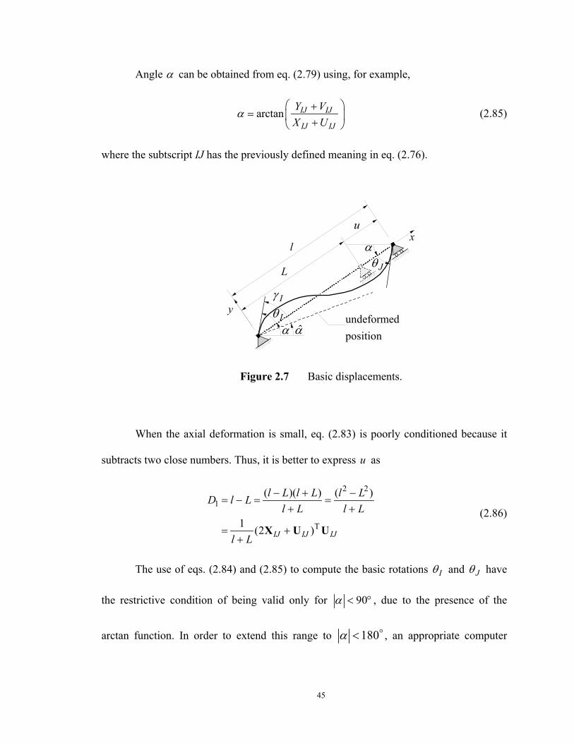
45

Angle α can be obtained from eq. (2.79) using, for example,

arctan IJ IJ

IJ IJ

Y VX U

α +

= + (2.85)

where the subtscript IJ has the previously defined meaning in eq. (2.76).

x

yIγ

α

u

L

α

l

Iθ

αJθ

undeformed position

Figure 2.7 Basic displacements.

When the axial deformation is small, eq. (2.83) is poorly conditioned because it

subtracts two close numbers. Thus, it is better to express u as

2 2

1

T

( )( ) ( )

1 (2 )IJ IJ IJ

l L l L l LD l Ll L l L

l L

− + −= − = =

+ +

= ++

X U U(2.86)

The use of eqs. (2.84) and (2.85) to compute the basic rotations Iθ and Jθ have

the restrictive condition of being valid only for 90α < ° , due to the presence of the

arctan function. In order to extend this range to 180α < , an appropriate computer

46

implementation of the arctan function2 can be used. The procedure presented in Crisfield

(1991) also has the same limitation, and the author recognizes the problem proposing a

solution that, in most circumstances, allows the extension of this range to 360 degrees.

In the present work a different procedure is proposed, such that there is no

limitation in the value of the rigid body rotation (as will be illustrated in Chapter 6).

Although the rotation of the element chord should not have any limitation in its

range, the basic rotations Iθ and Jθ can be assumed moderate. Taking advantage of this

assumption, the determination of the basic rotations can be performed as follows.

The first of eqs. (2.84) can be modified to

( )ˆsin sin ( ) sin( )cos sin sin cos

I I I

I I

θ γ α α β αα β α β

= + − = −

= −(2.87)

where

ˆI Iβ γ α= + (2.88)

Also,

( )ˆcos cos ( ) sin( )cos cos sin sin

I I I

I I

θ γ α α β αα β α β

= + − = −

= +(2.89)

Which allows for the computation of Iθ as

cos sin sin cosarctancos cos sin sin

I II

I I

α β α βθα β α β

−= +

(2.90)

2 In the majority of scientific programing languages, there is a convenient implementation of the

arc tangent function, usually denoted atan2(x,y), that allows for the determination of the quadrant

corresponding to the angle.

47

and similarly for the computation of Jθ as

cos sin sin cosarctancos cos sin sin

J JJ

J J

α β α βθα β α β

−= +

(2.91)

with

ˆJ Jβ γ α= + (2.92)

Thus, eqs. (2.90) and (2.91) employ the arctan function to determine small angles

(the basic rotations). By contrast, eqs. (2.84) and (2.85) use the arctan fuction (or the

usual computer implementation arctan2) to determine a angle (the rotation of the chord)

that can be arbitrarily large.

2.9.4 Transformation of forces

The forces in the global coordinate system are related to the forces in the basic system

through the following exact transformation, as deduced from Figure 2.8

1 1

2 1

3 2

4 1

5 1

6 3

ˆ cos sinˆ sin cosˆ

ˆ cos sinˆ sin cosˆ

P P Q

P P Q

P P

P P Q

P P Q

P P

α α

α α

α α

α α

= − −

= − +

=

= +

= −

=

(2.93)

where

2 3I JM M P PQl l+ +

= = (2.94)

is the shear force at the element ends (considering the deformed length in the basic

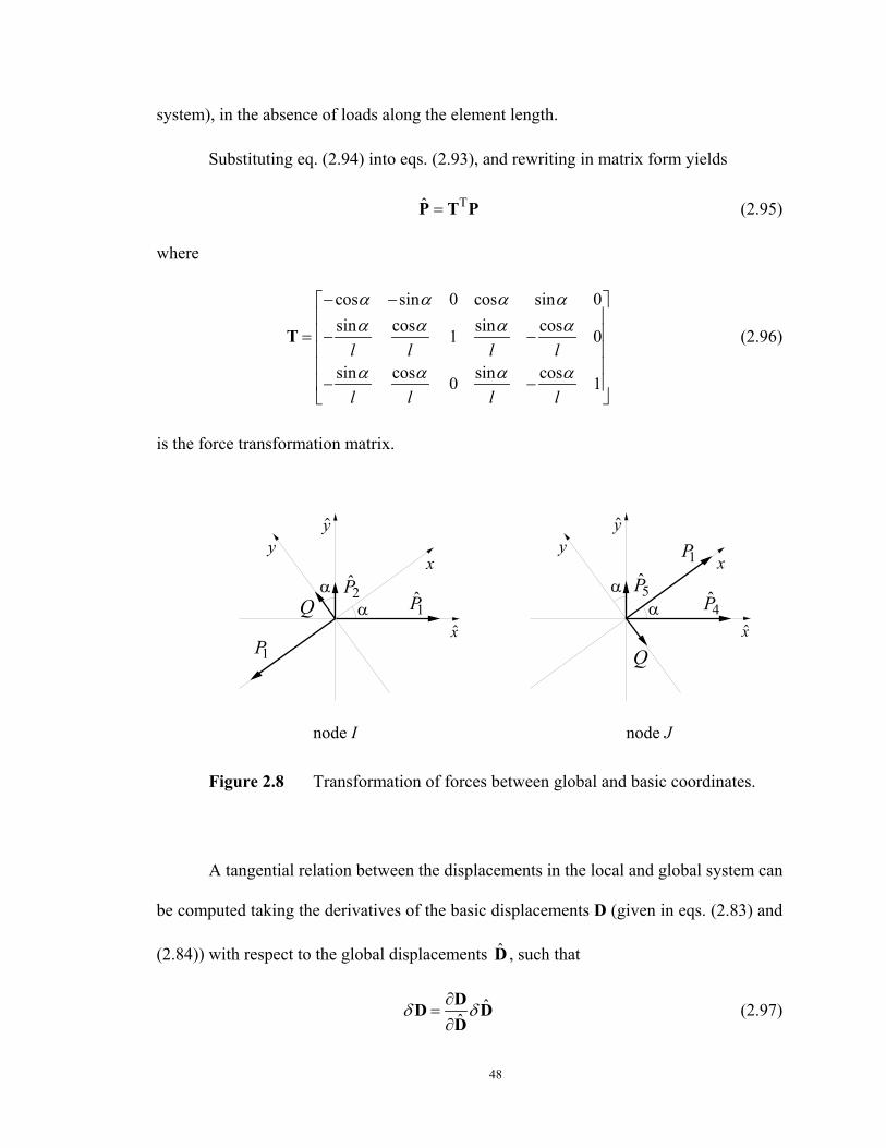
48

system), in the absence of loads along the element length.

Substituting eq. (2.94) into eqs. (2.93), and rewriting in matrix form yields

Tˆ =P T P (2.95)

where

cos sin 0 cos sin 0sin cos sin cos1 0

sin cos sin cos0 1

l l l l

l l l l

α α α αα α α α

α α α α

− − = − − − −

T (2.96)

is the force transformation matrix.

y

xQ

xy

αα

y

x

Q

xy

αα

1P2P

1P

5P4P

1P

node I node J

Figure 2.8 Transformation of forces between global and basic coordinates.

A tangential relation between the displacements in the local and global system can

be computed taking the derivatives of the basic displacements D (given in eqs. (2.83) and

(2.84)) with respect to the global displacements D , such that

ˆˆδ δ∂

=∂DD DD

(2.97)

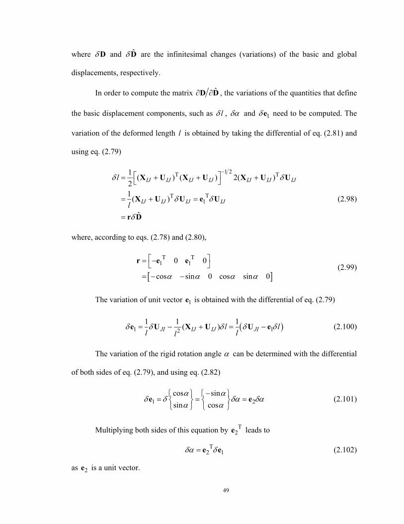
49

where δD and ˆδD are the infinitesimal changes (variations) of the basic and global

displacements, respectively.

In order to compute the matrix ˆ∂ ∂D D , the variations of the quantities that define

the basic displacement components, such as lδ , δα and 1δe need to be computed. The

variation of the deformed length l is obtained by taking the differential of eq. (2.81) and

using eq. (2.79)

1 2T T

TT1

1 ( ) ( ) 2( )21( )

ˆ

IJ IJ IJ IJ IJ IJ IJ

IJ IJ IJ IJ

l

l

δ δ

δ δ

δ

− = + + +

= + =

=

X U X U X U U

X U U e U

r D

(2.98)

where, according to eqs. (2.78) and (2.80),

[ ]

T T1 10 0

cos sin 0 cos sin 0α α α α

= − = − −

r e e(2.99)

The variation of unit vector 1e is obtained with the differential of eq. (2.79)

( )1 121 1 1( )JI IJ IJ JIl ll ll

δ δ δ δ δ= − + = −e U X U U e (2.100)

The variation of the rigid rotation angle α can be determined with the differential

of both sides of eq. (2.79), and using eq. (2.82)

1 2cos sinsin cos

α αδ δ δα δα

α α−

= = =

e e (2.101)

Multiplying both sides of this equation by T2e leads to

T2 1δα δ= e e (2.102)

as 2e is a unit vector.

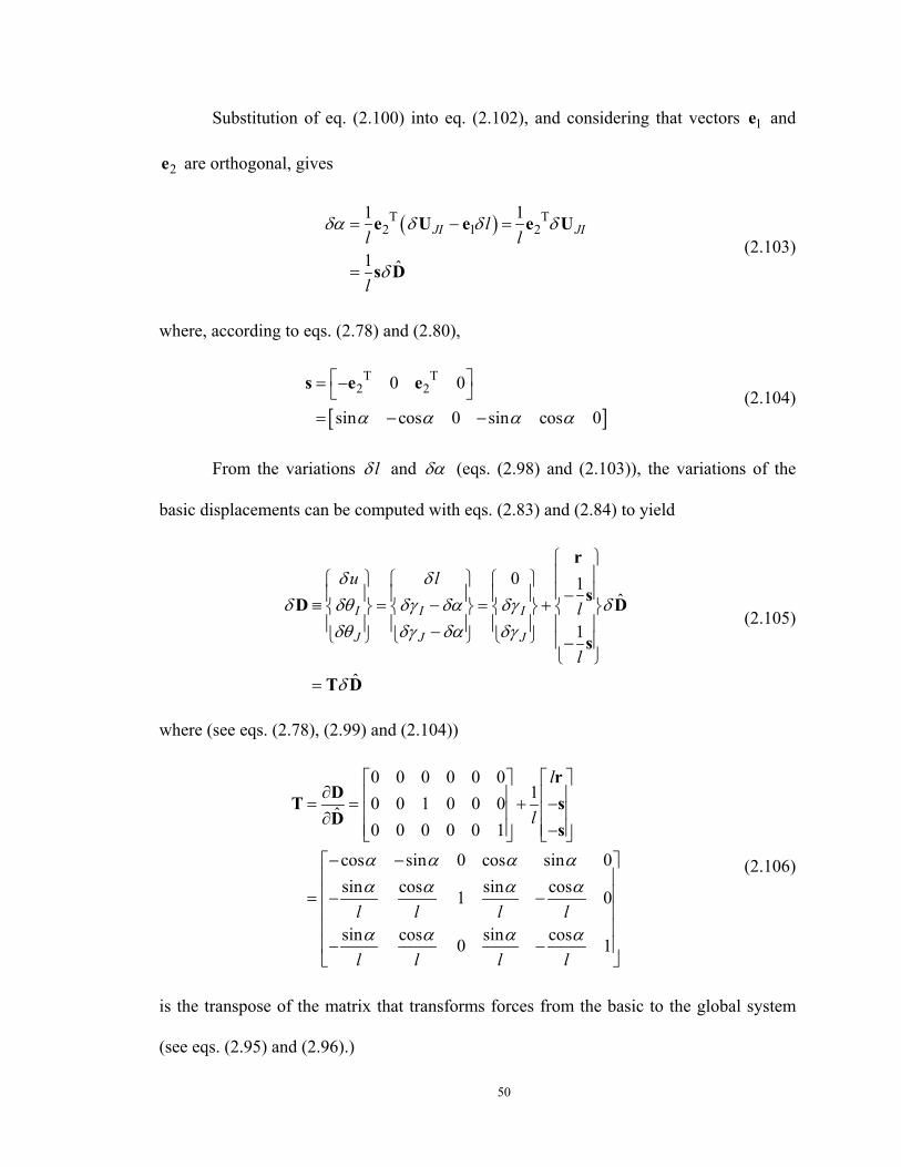
50

Substitution of eq. (2.100) into eq. (2.102), and considering that vectors 1e and

2e are orthogonal, gives

( )T T2 1 2

1 1

1 ˆ

JI JIll l

l

δα δ δ δ

δ

= − =

=

e U e e U

s D(2.103)

where, according to eqs. (2.78) and (2.80),

[ ]

T T2 20 0

sin cos 0 sin cos 0α α α α

= − = − −

s e e(2.104)

From the variations lδ and δα (eqs. (2.98) and (2.103)), the variations of the

basic displacements can be computed with eqs. (2.83) and (2.84) to yield

0 1ˆ

1

ˆ

I I I

J J J

u l

l

l

δ δδ δθ δγ δα δγ δ

δθ δγ δα δγ

δ

−≡ = − = +

− −

=

r

sD D

s

T D

(2.105)

where (see eqs. (2.78), (2.99) and (2.104))

0 0 0 0 0 010 0 1 0 0 0ˆ

0 0 0 0 0 1

cos sin 0 cos sin 0sin cos sin cos1 0

sin cos sin cos0 1

l

l

l l l l

l l l l

α α α αα α α α

α α α α

∂ = = + − ∂ − − − = − − − −

rDT sD s

(2.106)

is the transpose of the matrix that transforms forces from the basic to the global system

(see eqs. (2.95) and (2.96).)

51

This corresponds to an extension of the Principle of Contragradiency of structural

analysis, for the nonlinear geometric case. This principle can be derived from the

principle of virtual work, considering that the work performed by forces P going through

virtual displacements δD in the basic system, is equal to the work done by forces P

going through virtual displacements ˆδD in the global system. Therefore,

T T T Tˆ ˆ ˆδ δ δ= =D P D P D T P (2.107)

As the virtual work equation must hold for arbitrary virtual displacements δD ,

eq. (2.95) follows.

The transformations given by eqs. (2.83), (2.84) and (2.95) are exact. If other

approximate transformations for forces and displacements between the two systems of

coordinates are used, as in Neuenhofer and Filippou (1998), for instance, the relations

ˆδ δ=D T D and Tˆ =P T P need to be satisfied in order to maintain the symmetry of the

stiffness matrix with respect to the local coordinate system.

2.9.5 Tangent stiffness matrix in the global system

The element stiffness matrix in the basic coordinate system relates the displacement

increments to the force increments

δ δ=P K D (2.108)

and is obtained by inversion of the flexibility matrix, which is calculated according to

eq. (2.53)

1−=K F (2.109)

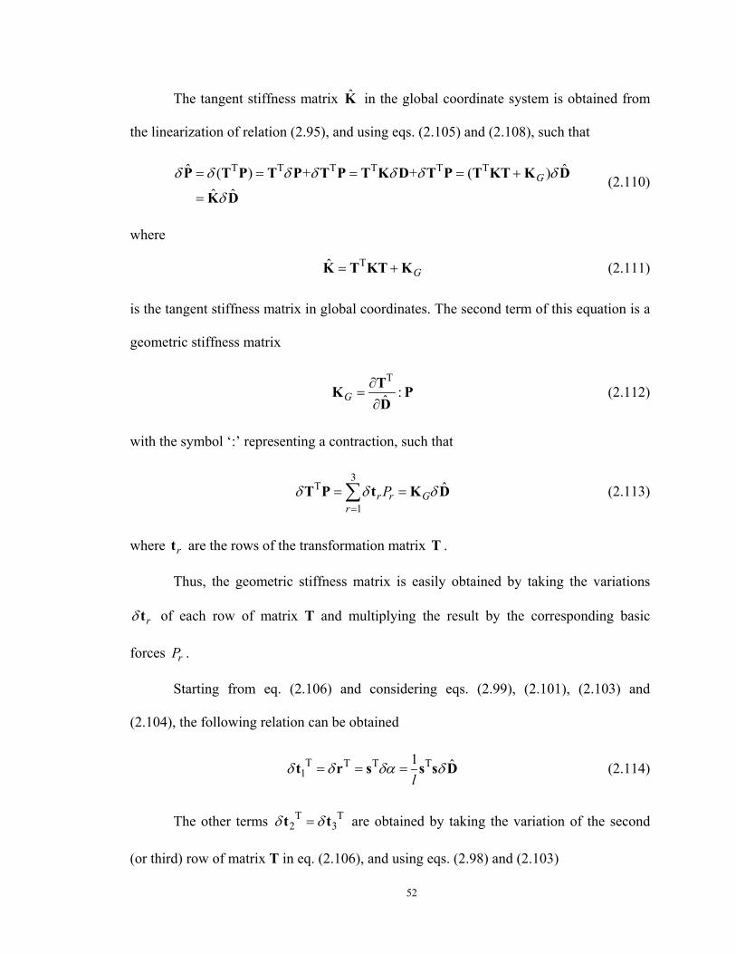
52

The tangent stiffness matrix K in the global coordinate system is obtained from

the linearization of relation (2.95), and using eqs. (2.105) and (2.108), such that

T T T T T Tˆ ˆ( ) + + ( )ˆ ˆ

Gδ δ δ δ δ δ δ

δ

= = = = +

=

P T P T P T P T K D T P T KT K D

K D(2.110)

where

TˆG= +K T KT K (2.111)

is the tangent stiffness matrix in global coordinates. The second term of this equation is a

geometric stiffness matrix

T:ˆG

∂=

∂TK PD

(2.112)

with the symbol ‘:’ representing a contraction, such that

3T

1

ˆr r G

rPδ δ δ

== =∑T P t K D (2.113)

where rt are the rows of the transformation matrix T .

Thus, the geometric stiffness matrix is easily obtained by taking the variations

rδ t of each row of matrix T and multiplying the result by the corresponding basic

forces rP .

Starting from eq. (2.106) and considering eqs. (2.99), (2.101), (2.103) and

(2.104), the following relation can be obtained

T T T T1

1 ˆl

δ δ δα δ= = =t r s s s D (2.114)

The other terms T T2 3δ δ=t t are obtained by taking the variation of the second

(or third) row of matrix T in eq. (2.106), and using eqs. (2.98) and (2.103)

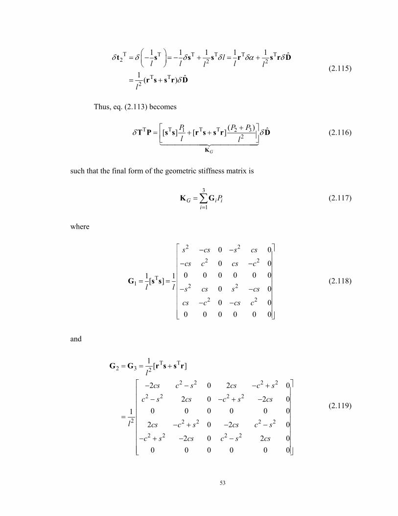
53

T T T T T T2 2 2

T T2

1 1 1 1 1 ˆ

1 ˆ( )

ll l ll l

l

δ δ δ δ δα δ

δ

= − = − + = +

= +

t s s s r s r D

r s s r D(2.115)

Thus, eq. (2.113) becomes

T T T T1 2 32

( ) ˆ[ ] [ ]

G

P P Pl l

δ δ+ = + + K

T P s s r s s r D (2.116)

such that the final form of the geometric stiffness matrix is

3

1G i i

iP

== ∑K G (2.117)

where

2 2

2 2

T1 2 2

2 2

0 0

0 00 0 0 0 0 01 1[ ]

0 0

0 00 0 0 0 0 0

s cs s cs

cs c cs c

l l s cs s cs

cs c cs c

− − − − = = − − − −

G s s (2.118)

and

T T2 3 2

2 2 2 2

2 2 2 2

2 2 2 2 2

2 2 2 2

1 [ ]

2 0 2 0

2 0 2 00 0 0 0 0 01

2 0 2 0

2 0 2 00 0 0 0 0 0

lcs c s cs c s

c s cs c s cs

l cs c s cs c s

c s cs c s cs

= = +

− − − + − − + − = − + − − − + − −

G G r s s r

(2.119)

54

with cosc α= and sins α= .

According to Kassimali (1983), the expression for the stiffness matrix (2.111) was

originally derived by Oran (1973a). As recognized by Crisfield (1990), Oran derived an

elegant and consistent tangent stiffness formulation in a two-dimensional context.

However, the earlier work by Powell (1969) presented a similar derivation.

It should be observed that for a symmetric stiffness matrix K in the basic system,

the global stiffness matrix K is symmetric, as matrices 1G and 2 3=G G are also

symmetric.

55

Chapter 3Large Rotations

This chapter describes an overview of the theory of large rotations in space. All the

formulae necessary in the development of the three-dimensional corotational formulation

to be presented in Chapter 4, such as rotation matrices and compound rotations are

derived and discussed here. A brief description of Euler parameters and unit quaternions

and their application in the update of rotational variables is also presented.

3.1 Rotation Matrix – Rodrigues Formula

Consider a vector 0v that defines the position of a point 0P with respect to a fixed

reference system ( , , )X Y Z , according to Figure 3.1.a. The vector 0v is to be rotated

about a unit vector t , by an angle θ , to a new vector 1v , which defines the position of

point 1P .

The following derivation was presented by Argyris (1982) and is also given in

Crisfield (1991).

Let ∆v be the vector connecting points 0P and 1P such that

1 0= + ∆v v v (3.1)

As point oP rotates about vector t, it describes a circle of radius r with center at

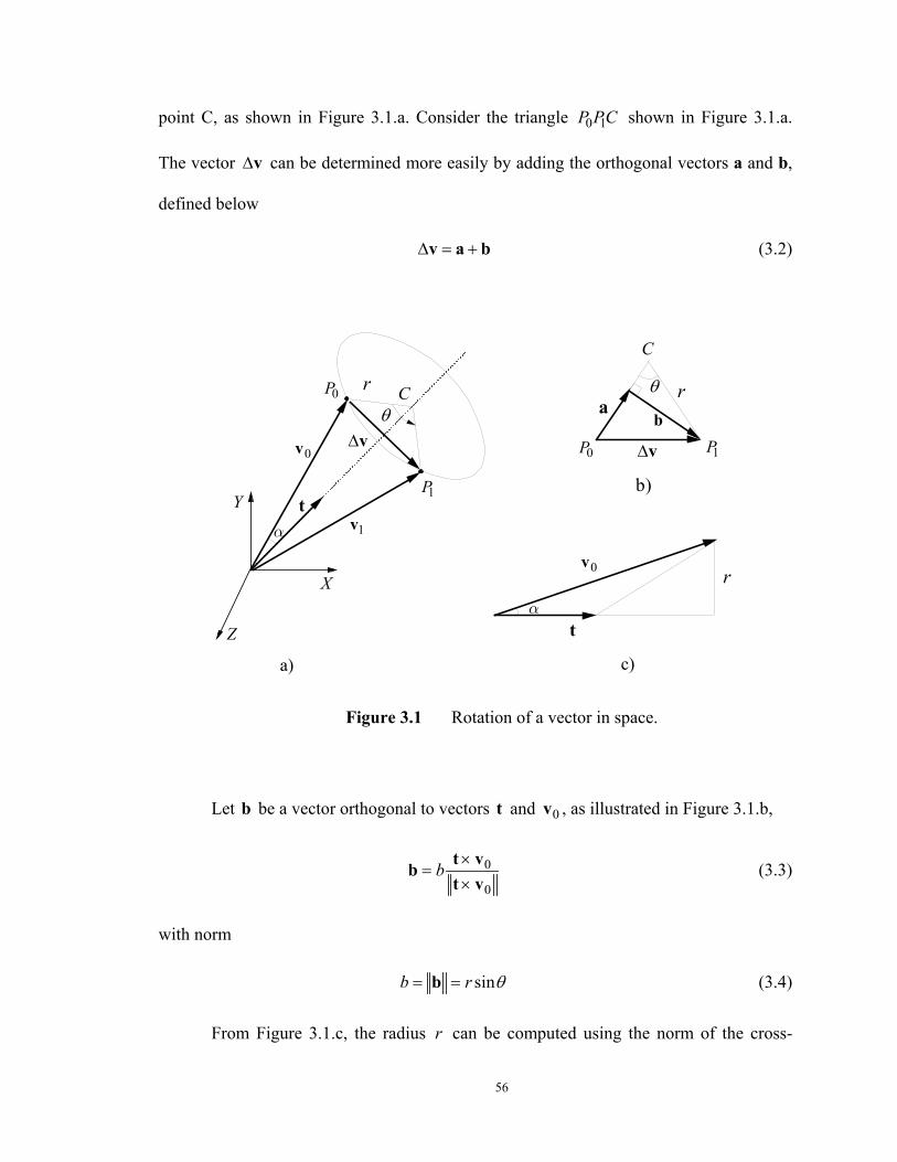
56

point C, as shown in Figure 3.1.a. Consider the triangle 0 1P PC shown in Figure 3.1.a.

The vector ∆v can be determined more easily by adding the orthogonal vectors a and b,

defined below

∆ = +v a b (3.2)

X

Y

a

1v

Z

tα

C

0P

1P

θv∆

r

v∆

r

0v

θ

b

1P0P

C

αt

0vr

a)

b)

c)

Figure 3.1 Rotation of a vector in space.

Let b be a vector orthogonal to vectors t and 0v , as illustrated in Figure 3.1.b,

0

0b ×

=×

t vbt v

(3.3)

with norm

sinb r θ= =b (3.4)

From Figure 3.1.c, the radius r can be computed using the norm of the cross-

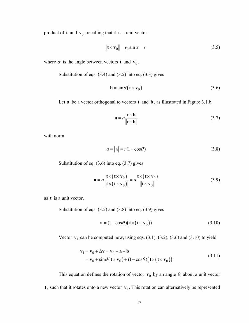
57

product of t and 0v , recalling that t is a unit vector

0 0 sinv rα× = =t v (3.5)

where α is the angle between vectors t and 0v .

Substitution of eqs. (3.4) and (3.5) into eq. (3.3) gives

( )0sinθ= ×b t v (3.6)

Let a be a vector orthogonal to vectors t and b , as illustrated in Figure 3.1.b,

a ×=

×t bat b

(3.7)

with norm

(1 cos )a r θ= = −a (3.8)

Substitution of eq. (3.6) into eq. (3.7) gives

( )( )

( )0 0

00a a

× × × ×= =

×× ×t t v t t v

at vt t v

(3.9)

as t is a unit vector.

Substitution of eqs. (3.5) and (3.8) into eq. (3.9) gives

( )( )0(1 cos )θ= − × ×a t t v (3.10)

Vector 1v can be computed now, using eqs. (3.1), (3.2), (3.6) and (3.10) to yield

( ) ( )( )1 0 0

0 0 0sin (1 cos )θ θ

= + ∆ = + +

= + × + − × ×

v v v v a b

v t v t t v(3.11)

This equation defines the rotation of vector 0v by an angle θ about a unit vector

t , such that it rotates onto a new vector 1v . This rotation can alternatively be represented

58

by a ‘pseudo-vector’ θ (Argyris (1982)).

[ ]1 2 3θ θ θ θ= =Tθ t (3.12)

which is parallel to vector t , and with norm equal to the rotation angle

θ=θ (3.13)

The term ‘pseudo-vector’ emphasizes the fact that rotations do not satisfy all

vector properties. An alternative name for the term ‘pseudo-vector’, very often used in

the literature, is ‘rotational vector’. It should be noted that, while for infinitesimal

rotations, components 1θ , 2θ and 3θ can be considered as component rotations about

axes X, Y and Z, this is not the case for finite rotations.

With eq. (3.12) eq. (3.11) can be expressed as

( ) ( )( )1 0 0 02sin (1 cos )θ θθ θ

−= + × + × ×v v θ v θ θ v (3.14)

The cross product of two vectors can also be expressed in the form

2 3 3 2

3 1 1 3

1 2 2 1

( )w v w vw v w vw v w v

− × = − = −

w v S w v (3.15)

where

3 2

3 1

2 1

0( ) spin( ) 0

0

w ww ww w

− ≡ = − −

S w w (3.16)

is a skew symmetric matrix, which is also used to represent infinitesimal rotations about

orthogonal axes. Due to this relation, a skew symmetric matrix ( )S w is often referred to

as the ‘spin tensor’, with the associated vector w being the ‘axial vector’ or ‘spin axis’.

59

The following notation is commonly used in the literature to refer to the ‘inverse’ of

relation (3.16)

32 23

13 31

21 12

axial( )S SS SS S

≡ = = −

w S (3.17)

The square of the skew symmetric matrix is a symmetric matrix and can be

expressed as

2 T T

T

( ) ( ) ( ) ( )

w

= = −

= −

S w S w S w ww w w I

ww I(3.18)

Using eq. (3.15), eq. (3.14) can be rewritten as

1 0 0 02sin (1 cos )( ) ( ) ( )θ θθ θ

−= + +v v S θ v S θ S θ v (3.19)

or in more compact form,

1 0( )=v R θ v (3.20)

where

22

2

sin (1 cos )( ) ( ) ( )

sin ( ) (1 cos ) ( )

θ θθ θθ θ

−= + +

= + + −

R θ I S θ S θ

I S t S t(3.21)

is the rotation matrix, with I being the 3 3× identity matrix. This is the so-called

Rodrigues formula.

In the limit when 0θ → , the infinitesimal rotational formula can be recovered

from eq. (3.21) as

( ) ( )= +R θ I S θ (3.22)

60

An alternative form for the rotation formula can be obtained using the series

expansion of the trigonometric functions

3 5 7 (2 1)1 1 1 1sin ( 1)3! 5! 7! (2 1)!

n n

nθ θ θ θ θ θ += − + − + + − +

+(3.23)

2 4 6 21 1 1 1cos 1 ( 1)2! 4! 6! (2 )!

n n

nθ θ θ θ θ= − + − + + − + (3.24)

which, in conjunction with eq. (3.21) gives

2 4 2

2 4 2 2

1 1 1( ) 1 ( 1) ( )3! 5! (2 1)!

1 1 1 1( 1) ( )2! 4! 6! (2 2)!

n n

n n

n

n

θ θ θ

θ θ θ

= + − + + + − + +

+ − + − + − + +

R θ I S θ

S θ(3.25)

The powers of S can be computed using simple matrix multiplication (see eq.

(3.16)), and result in the following relations

3 2 4 2 2

5 4 6 4 2

θ θ

θ θ

= − = −

= + = +

S S S S

S S S S(3.26)

which leads to the recurrence formulae

2 1 1 2( 1)

2 1 2( 1) 2

( 1)

( 1)

n n n

n n n

θ

θ

− − −

− −

= −

= −

S S

S S(3.27)

Substitution of these equations in (3.25) gives

2 31 1 1( ) ( ) ( ) ( ) ( )2! 3! !

n

n= + + + + + +R θ I S θ S θ S θ S θ (3.28)

which corresponds to the exponential mapping of the skew symmetric matrix S

( )( ) exp( ( )) e= = S θR θ S θ (3.29)

61

An alternative form for the rotation matrix is obtained using a modified form of

the pseudo-vector θ

tan( 2)2 tan( 2) 2 θω θθ

= = =ω t t θ (3.30)

where ω is the so called tangent-scaled pseudo vector. Its components are also referred

to as Rodrigues parameters. The problem with this form of the pseudo-vector is that it

becomes infinite for nθ π= (with 1,2,...n = ).

In order to express the rotation matrix in terms of the tangent-scaled pseudo

vector, the following half angle formulas for cosine and sine are necessary

2 2 2cos cos ( 2) sin ( 2) 1 2sin ( 2)sin 2cos( 2)sin( 2)

θ θ θ θθ θ θ= − = −=

(3.31)

Substitution of eq. (3.31) into eq. (3.21) gives

2 22sin( 2)cos( 2) ( ) 2sin ( 2) ( )θ θ θ= + +R I S t S t (3.32)

Substitution of eq. (3.30) into eq. (3.32) leads to

2 21cos ( 2) ( ) ( )2

θ = + + R I S ω S ω (3.33)

However,

22

1cos ( 2)1 tan ( 2)

θθ

=+

(3.34)

and

T 2 T 24 tan ( 2) 4 tan ( 2)θ θ= =ω ω t t (3.35)

Thus, eq. (3.33) becomes

62

14

1 1( ) ( ) ( )21

= + + + TR I S ω S ω S ωω ω

(3.36)

3.2 Extraction of the rotational vector from the rotation matrix

In some cases, it is necessary to compute the rotational vector that corresponds to a given

rotation matrix. The rotational vector θ can be extracted from the anti-symmetric part of

the rotation matrix R

a T1 sin( ) ( ) sin ( )2

θ θθ

= − = =R R R S θ S t (3.37)

since 2S is a symmetric matrix.

Let τ be defined as the axial vector of aR , the anti-symmetric part of R (see eqs.

(3.16), (3.17) and (3.37))

a T1 sinaxial( ) axial ( ) axial ( )2

sin sin

θθ

θ θθ

= = − =

= =

τ R R R S θ

θ t(3.38)

The norm of τ is

sin sinτ θ θ= = =τ t (3.39)

since 1=t .

The pseudo-vector can be written implicitly in terms of the components of R as

32 23T

13 31

21 12

sin 1 1sin axial( )2 2

R RR RR R

θ θθ

− = = = − = − −

θ t τ R R (3.40)

63

or can be given explicitly, using eqs. (3.38) and (3.39), such that

TT

T

arcsinsin

1 axial( )arcsin axial( )2 axial( )

θ τθ τ

= =

− = − −

τθ τ

R RR RR R

(3.41)

It is observed that, due to the presence of the arcsin function, this equation is

limited to angles 90θ ≤ ° .

3.3 Euler parameters and normalized quaternions

As discussed previously there are many forms to represent (and store) a rotation. One can

for example, store nine parameters corresponding to the whole rotation matrix.

Alternatively, due to the orthonormality condition of the rotation matrix, a rotation can

also be represented in terms of only three components of the rotational vectors, or in

terms of the Rodrigues parameters (tangent-scaled pseudo-vector).

However, there are difficulties in obtaining these parameters from the rotation

matrix, for angles equal or greater than 180°. A better approach is to use Euler

parameters, represented in terms of unit quaternions (which have four components). The

use of Euler parameters and quaternions in the manipulation of finite rotations is

investigated in Spring (1986).

According to Spring, the algebra of quaternions was introduced by Hamilton over

a century ago, but has only recently been put to practical application with its increased

use in the aerospace industry.

The normalized quaternion can represent a ‘sine-scaled’ pseudo-vector in the

64

same direction of t , but with norm sin( 2)θ ,

sin( 2)θ=q t (3.42)

plus an additional parameter

0 cos( 2)θ=q (3.43)

which can be used to provide extra information in the determination of the angle θ from

the rotation matrix.

These four parameters are the so-called Euler parameters, and can be grouped and

represented in vector form as

0

1 0

2

3

cos( 2)cos( 2)sin( 2) sin( 2)

qq qqq

θθθ θ

θ

= = = =

θq tq (3.44)

The meaning of the term ‘normalized’ quaternion becomes clear by the fact that,

according to eq. (3.44), the norm of q is equal to one

2 2 2 2T0 1 2 3

2 2 Tcos ( 2) sin ( 2) 1

q q q q

θ θ

= + + +

= + =

q q

t t(3.45)

Substitution of eqs. (3.31) into eq. (3.21) gives

( ) ( ) ( ) ( )2 2 2( ) 2cos 2 sin 2 ( ) 1 cos 2 sin 2 ( )θ θ θ θ = + + − + R θ I S t S t (3.46)

From eq.(3.18), the term 2( )S t can be rewritten as

2 T( ) = −S t tt I (3.47)

Thus, eq. (3.46) becomes

65

( ) ( ) ( ) ( )

( )

2 2

2 T

( ) cos 2 sin 2 2cos 2 sin 2 ( )

2sin 2

θ θ θ θ

θ

= − + +

R θ I S t

tt(3.48)

Substitution of eqs. (3.42) and (3.43) into eq. (3.48) leads to

( )( )

2 T T0 0

2 T0 0

2 ( ) 2

2 1 2 ( ) 2

q q

q q

= − + +

= − + +

R q q I S q qq

I S q qq(3.49)

which, in expanded form, becomes

2 20 1 1 2 0 3 1 3 0 2

2 22 1 0 3 0 2 2 3 1 0

2 23 1 0 2 3 2 0 1 0 3

1 2

2 1 2

1 2

q q q q q q q q q q

q q q q q q q q q q

q q q q q q q q q q

+ − − + = + + − −

− + + −

R (3.50)

3.4 Compound rotations

As discussed before, the result of successive rotations applied to a body depends on the

order in which the rotations are applied. Consequently, rotations do not follow the rules

established for vectors.

One important problem about large rotations, consists in the successive

applications of rotations on a body. Consider for example, the case in which one vector

0v is rotated to a vector 1v using a pseudo vector 1θ and then is rotated to another vector

2v using another pseudo vector 2θ

1 1 0

2 2 1

( )( )

==

v R θ vv R θ v

(3.51)

66

Consequently, the final expression for vector 2v , starting from vector 0v is

2 2 1 0

2 1 0

( ) ( )( )

=≠ +

v R θ R θ vR θ θ v

(3.52)

Although the rotation update can be done multiplying two consecutive rotation

matrices according to eq. (3.52), a more efficient expression is obtained with quaternions

(Spring (1986))

2 2 1 0

12 0

( ) ( )

( )

=

=

v R R v

R v

q q

q(3.53)

where

T1 2 1 20 0

12 2 11 2 2 1 1 20 0

q qq q

− = = + − ×

q qq q q q

q q q (3.54)

is the quaternion product. It should be noted that this operation is not commutative, due

to the presence of the vector cross-product, i.e.,

T T1 2 1 2 1 2 1 20 0 0 0

1 21 2 2 1 2 1 1 2 2 1 1 20 0 0 0

2 1

q q q qq q q q

− − = = + − × + + ×

≠

q q q qq q q q q q q q

q q

q q

(3.55)

3.5 Extraction of the unit quaternion from the rotation matrix

In this formulation, and in other practical problems, it is necessary that the normalized

quaternion be computed from the rotation matrix. This can be easily accomplished due to

the form of the rotation matrix written in terms of the quaternion components (see

eq. (3.50)).

67

The term 0q can be obtained by computing the trace of the rotation matrix

2 2 2 2 20 1 2 3 0

20

tr( ) 2 3 3 2 2 2 1 2

4 1

q q q q q

q

= + + + − = −

= −

R(3.56)

according to eq. (3.45) and (3.50). Solving eq. (3.56) for 0q gives

01 tr( ) 12

q = +R (3.57)

The other components can be easily obtained by computing the anti-symmetric

part of R , using eq. (3.49) and noting that I and Tqq are symmetric matrices.

Accordingly,

3 2T

0 0 3 1

2 1

01 ( ) 2 ( ) 2 02

0

q qq q q q

q q

− − = = − −

R R S q (3.58)

whose solution is

1 32 23

2 13 310

3 21 12

14

q R Rq R R

qq R R

− = − −

(3.59)

or, alternatively,

( )0

14i k j jkq R R

q= − (3.60)

where i, j, k form a cyclic permutation of 1, 2, 3. This procedure, presented by Grubin

(1970), has a strong limitation, as eq. (3.60) reduces to 0/0 for 0 0q = , i.e, for an angle

180θ = , being also very inaccurate in the vicinity of this angle. An improved algorithm

is proposed in Klumpp (1976), such that this singularity is overcome. However, Spurrier

68

(1978) shows that the algorithm proposed by Klumpp is sensitive to numerical

imprecision whenever any quaternion component is small. Spurrier presented a better

algorithm, which always provides great accuracy, by using the square-root operation to

compute only the largest component, and by using only this component as a divisor in

computing the other components. Due to its robustness, this algorithm has been used in

several papers in the field of large rotation finite element analysis (see for example, Simo

and Vu-Quoc (1986), Crisfield (1990) and Nour-Omid and Rankin (1991)).

The algorithm proposed by Spurrier computes the largest (algebraically) of tr( )R ,

11R , 22R and 33R . If tr( )R is the largest term, then it computes the quaternion

components using eqs. (3.57) and (3.60). Otherwise it uses alternative expressions for the

sake of numerical accuracy, which are derived as follows. From eqs. (3.50) and (3.57), it

is observed that

[ ]

[ ]

2 2 20

2

12 2 1 2 1 tr( ) 12

12 tr( ) 12

ii i i

i

R q q q

q

= + − = + + −

= + −

R

R(3.61)

Thus, for any component iq (with 0i ≠ )

[ ]1 1 1 tr( )2 4i iiq R= + − R (3.62)

Spurrier suggests that eq. (3.62) be used for the computation of the component iq

corresponding to the largest iiR of the three diagonal elements.

The component 0q is computed using the inverse form of eq. (3.60)

( )01

4 k j jki

q R Rq

= − (3.63)

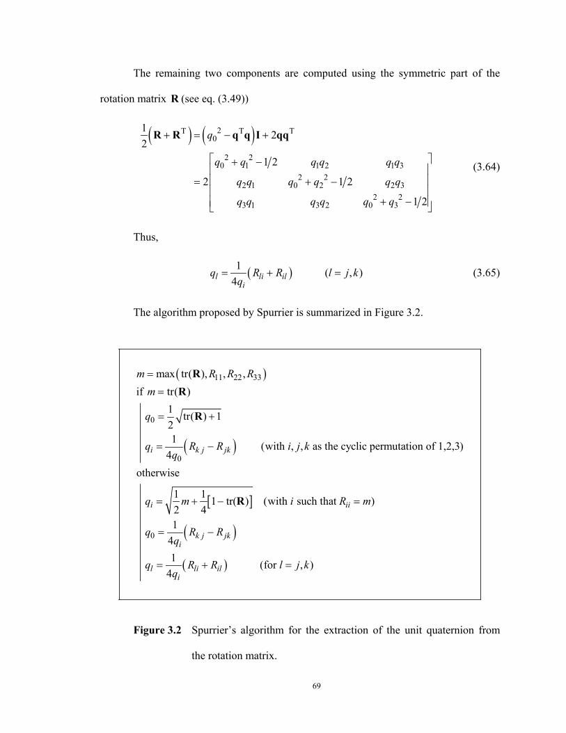
69

The remaining two components are computed using the symmetric part of the

rotation matrix R (see eq. (3.49))

( ) ( )2T T T0

2 20 1 1 2 1 3

2 22 1 0 2 2 3

2 23 1 3 2 0 3

1 22

1 2

2 1 2

1 2

q

q q q q q q

q q q q q q

q q q q q q

+ = − +

+ − = + −

+ −

R R q q I qq

(3.64)

Thus,

( )1 ( , )4l li il

iq R R l j k

q= + = (3.65)

The algorithm proposed by Spurrier is summarized in Figure 3.2.

( )

( )

[ ]

( )

( )

11 22 33

0

0

0

max tr( ), , ,if tr( )

1 tr( ) 121 (with , , as the cyclic permutation of 1,2,3)

4otherwise

1 1 1 tr( ) (with such that )2 41

41 (for , )

4

i k j jk

i ii

k j jki

l li ili

m R R Rm

q

q R R i j kq

q m i R m

q R Rq

q R R l j kq

=

=

= +

= −

= + − =

= −

= + =

RR

R

R

Figure 3.2 Spurrier’s algorithm for the extraction of the unit quaternion from

the rotation matrix.

70

From eq. (3.50) it is observed that if the sign of the unit quaternion q is switched,

the rotation matrix remains unchanged, as all the terms in this matrix are formed by the

square of the components of the unit quaternion, or by the product two components.

Therefore, a positive and a negative quaternion may be extracted from the same rotation

matrix.

After the normalized quaternion corresponding to the Euler parameters have been

obtained, the tangent scaled pseudo vector can be computed as (see eqs. (3.30) and

(3.44))

0

2 22 tan( 2)cos( 2) q

θθ

= = =ω t q q (3.66)

It is observed from this equation, that the tangent scaled pseudo vector does not

depend on the sign of the unit quaternion (due to the ratio 0qq ).

The extraction of the pseudo-vector θ from the unit quaternion, using eq. (3.44),

however is not unique, due to the use of the arccos and arcsin functions.

Jelenic and Crisfield (1998) propose a procedure for the unique extraction of the

rotational vector from the unit quaternion, whereby the rotational vector satisfies

180θ ≤ . This is accomplished by choosing the sign of the associated quaternion, such

that 0 0q ≥ . The proposed implementation also tries to minimise the round-off errors in

the extraction procedure by alternating the use of the arcsin and arccos, when it is more

appropriate. The pseudo code of the procedure is shown in Figure 3.3.

The great advantage of this procedure in comparison to eq. (3.41) is that it is

based on the arcsin (or arccos) of ( 2)θ (see eq. (3.44)), as opposed to the arcsin of θ .

Thus, instead of being applicable only to rotations in the range [ 2, 2]π π− + as in

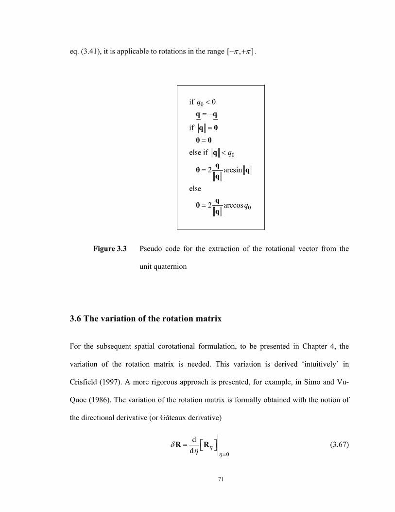
71

eq. (3.41), it is applicable to rotations in the range [ , ]π π− + .

0

0

0

if 0

if

else if

2 arcsin

else

2 arccos

q

q

q

<= −

=

=

<

=

=

0θ 0

θ

θ

q q

q

qq qq

qq

Figure 3.3 Pseudo code for the extraction of the rotational vector from the

unit quaternion

3.6 The variation of the rotation matrix

For the subsequent spatial corotational formulation, to be presented in Chapter 4, the

variation of the rotation matrix is needed. This variation is derived ‘intuitively’ in

Crisfield (1997). A more rigorous approach is presented, for example, in Simo and Vu-

Quoc (1986). The variation of the rotation matrix is formally obtained with the notion of

the directional derivative (or Gâteaux derivative)

0

dd η

ηδ

η =

= R R (3.67)

72

where ηR is the ‘perturbed’ rotation matrix R, computed according to the equation for

compound rotations (see eq. (3.52))

( ) ( ) exp( ( )) ( )η ηδ η δ= =R R θ R θ S θ R θ (3.68)

according to eq. (3.29).

Substitution of eq. (3.68) into eq. (3.67) gives

[ ] [ ]

[ ]0 0

0

d dexp( ( )) ( ) exp( ( )) ( )d d

( )exp( ( )) ( )

( ) ( )

η η

η

δ ηδ η δη η

δ η δ

δ

= =

=

= =

=

=

R S θ R θ S θ R θ

S θ S θ R θ

S θ R θ

(3.69)

3.7 Rotation of a triad via the smallest rotation

In the corotational formulation presented in the next chapter it will be necessary to rotate

a triad 1 2 3[ ]=P p p p such that one of its unit vectors, say 1p , coincides with another

independent unit vector, say 1e , via the smallest possible rotation. This is accomplished

by rotating the triad about a unit vector t that is orthogonal to both vectors 1p and 1e

1 1

1 1

×=

×p etp e

(3.70)

The rotation angle θ between the two unit vectors 1p and 1e is defined from the

dot product and cross product of these vectors

T1 1cosθ = p e (3.71)

1 1sinθ = ×t p e (3.72)

73

The rotation vector is obtained by multiplying vector t by angle θ

1 1

1 1θ θ ×

= =×

p eθ tp e

(3.73)

Substitution of eqs. (3.71) and (3.72) into eq. (3.21) leads to

1 1 1 1 1 12

1 1 1 1 1 1T1 1

(1 cos )( ) ( ) ( )sin

1( ) ( ) ( )1

θθ

−= + × + × ×

= + × + × ×+

R I S p e S p e S p e

I S p e S p e S p ep e

(3.74)

Consider a triad 1 2 3[ ]=E e e e that corresponds to the final position of triad P

after it has been rotated about the unit vector t, orthogonal to both 1p and 1e , by the

smallest angle θ

1 2 3 1 2 3[ ] [ ]= = =E e e e R p p p RP (3.75)

with matrix R being computed from eq. (3.74).

Since the vector 1p has to be rotated onto 1e , the relation

1 1=e Rp (3.76)

can be easily verified, as shown in Appendix B.

The derivation of the expressions for the other components 2e and 3e involves

lengthy algebraic manipulation, and thus, is presented in Appendix B. The final results

are

T2 1

2 2 1 1T1 1

( )1

= − ++

p ee p p ep e

(3.77)

T3 1

3 3 1 1T1 1

( )1

= − ++

p ee p p ep e

(3.78)

74

Chapter 4Space Element Formulation

This chapter describes the spatial element formulation. It has the same organization of

Chapter 2, without repeating the discussions about the common theoretical developments.

However, this chapter presents a more detailed discussion about the corotational

formulation due to the increased degree of complexity in three dimensions.

4.1 Coordinate systems

As in the planar case, the space element is formulated in a basic system (x, y, z) without

rigid body modes. This system is represented in Figure 4.1.

The element has six degrees of freedom in the chosen basic coordinate system:

one relative axial displacement Ju , two rotations relative to the chord I zθ and J zθ ,

about the z axis, two rotations relative to the chord I yθ and J yθ , about the y axis, and

one relative angle of twist Jψ . These relative displacements correspond to the minimum

number of geometric variables necessary to describe the deformation modes of the

element in space. The six statically independent end forces related to these displacements

are the axial force JN , the bending moments in the xy plane, I zM and J zM , the two

bending moments in the xz plane, I yM and J zM , and the torsional moment JT . These

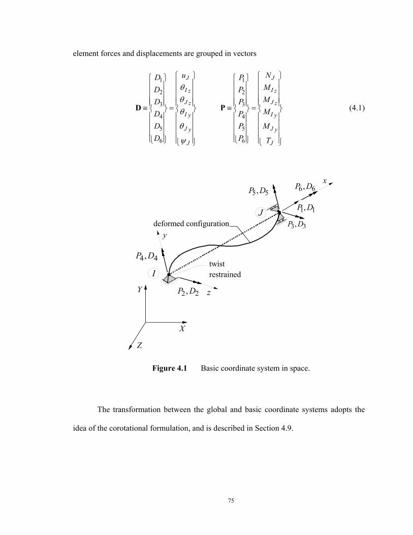
75

element forces and displacements are grouped in vectors

1 1

2 2

3 3

4 4

5 5

6 6

J J

I Iz z

J Jz z

I Iy y

J Jy y

J J

u ND PMD PMD PMD PMD P

D P T

θθθ

θ

ψ

≡ = ≡ =

D P (4.1)

4 4,P D

x

ydeformed configuration

X

Y

Z

2 2,P D z

5 5,P D

3 3,P D

1 1,P D

6 6,P D

J

Itwist restrained

Figure 4.1 Basic coordinate system in space.

The transformation between the global and basic coordinate systems adopts the

idea of the corotational formulation, and is described in Section 4.9.

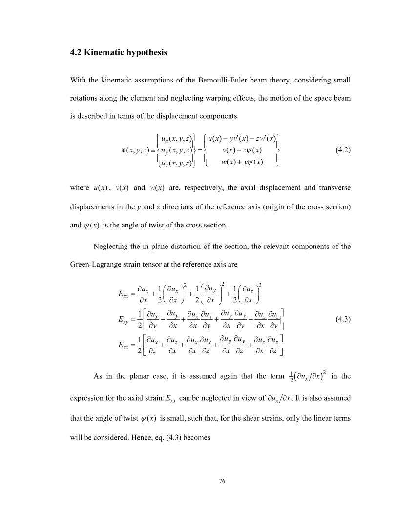
76

4.2 Kinematic hypothesis

With the kinematic assumptions of the Bernoulli-Euler beam theory, considering small

rotations along the element and neglecting warping effects, the motion of the space beam

is described in terms of the displacement components

( , , ) ( ) ( ) ( )( , , ) ( , , ) ( ) ( )

( ) ( )( , , )

x

y

z

u x y z u x yv x zw xx y z u x y z v x z x

w x y xu x y z

ψψ

′ ′− − ≡ = − +

u (4.2)

where ( )u x , ( )v x and ( )w x are, respectively, the axial displacement and transverse

displacements in the y and z directions of the reference axis (origin of the cross section)

and ( )xψ is the angle of twist of the cross section.

Neglecting the in-plane distortion of the section, the relevant components of the

Green-Lagrange strain tensor at the reference axis are

22 21 1 12 2 2

12

12

yx x zxx

y y yx x x z zxy

y yx z x x z zxz

uu u uEx x x x

u u uu u u u uEy x x y x y x y

u uu u u u u uEz x x z x z x z

∂ ∂ ∂ ∂ = + + + ∂ ∂ ∂ ∂ ∂ ∂ ∂ ∂ ∂ ∂ ∂ ∂

= + + + + ∂ ∂ ∂ ∂ ∂ ∂ ∂ ∂ ∂ ∂ ∂ ∂ ∂ ∂ ∂ ∂

= + + + + ∂ ∂ ∂ ∂ ∂ ∂ ∂ ∂

(4.3)

As in the planar case, it is assumed again that the term ( )212 xu x∂ ∂ in the

expression for the axial strain xxE can be neglected in view of xu x∂ ∂ . It is also assumed

that the angle of twist ( )xψ is small, such that, for the shear strains, only the linear terms

will be considered. Hence, eq. (4.3) becomes

77

2 21 12 2

12

12

yx zxx

yxxy

x zxz

uu uEx x x

uuEy x

u uEz x

∂ ∂ ∂≅ + + ∂ ∂ ∂

∂ ∂≅ + ∂ ∂

∂ ∂≅ + ∂ ∂

(4.4)

Taking the derivatives of the displacement field (4.2) with respect to x, y and z,

substituting the results in eq. (4.4) gives

( ) ( )2 21 1( , , ) ( ) ( ) ( ) ( ) ( ) ( ) ( )2 2

1( , , ) ( )2

1( , , ) ( )2

xx

xy

xz

E x y z u x yv x zw x v x z x w x y x

E x y z z x

E x y z y x

ψ ψ

ψ

ψ

′ ′′ ′′ ′ ′ ′ ′≅ − − + − + +

′≅ −

′≅

(4.5)

Neglecting the effects of torsion in the axial strains, i.e., assuming that the terms

( )xψ′ can be neglected in the equation for xxE , the strains at a point ( , , )x y z of the

cross-section can be expressed as

0( , , ) ( ) ( ) ( )

1( , , ) ( )2

1( , , ) ( )2

xx z y

xy

xz

x y z x y x z x

x y z z x

x y z y x

ε ε κ κ

ε ϕ

ε ϕ

= − +

= −

=

(4.6)

where

( ) ( )2 20

1 1( ) ( ) ( ) ( )2 2

( ) ( )( ) ( )

( ) ( )

z

y

x u x v x w x

x v xx w x

x x

ε

κκ

ϕ ψ

′ ′ ′= + +

′′=′′= −

′=

(4.7)

are the axial strain at a reference axis, the curvatures of the cross-section with respect to

78

the z and y axes, and the angle of twist per unit length, respectively.

With the simplification in the axial strains, the terms ( )212 ( )v x′ and ( )21

2 ( )w x′ are

responsible for representing the second-order effects in the adopted strain-displacement

relation. It is observed that the assumptions discussed above lead to a geometrically linear

torsional behavior, uncoupled from the flexural and axial behavior of the beam3.

However, these assumptions are appropriate for structures in the range of moderately

large deformations where the most important non-linear geometric effect is the second-

order bending moment due to axial force.

This type of structures comprises the target problems of this space formulation.

Nonetheless, the proposed element is able to solve problems with large deformations

(even with relatively large angle of twist, such as in lateral and torsional buckling

problems). This is accomplished by using the corotational formulation and subdividing

the structural member into smaller sub-elements. Some examples of this type of problems

will be analyzed in Chapter 6.

Eq. (4.6) can be rewritten in matrix form as

( , , )( , , ) 2 ( , , ) ( , ) ( )

2 ( , , )

xx

xy

xz

x y zx y z x y z y z x

x y z

εε

ε

≡ =

ε a d (4.8)

where

T0( ) ( ) ( ) ( ) ( )z yx x x x xε κ κ ϕ=d (4.9)

3 Strictly speaking, the mentioned uncoupled behavior applies to beams with elastic material. In

general, the torsional and flexural behavior may be coupled through the section constitutive relation.

79

are the generalized section strains or section deformations, and

1 0( , ) 0 0 0

0 0 0

y zy z z

y

− = −

a (4.10)

is a matrix that relates the section deformations with the strains at a point of the cross-

section.

It should be noted that the shear strains were multiplied by the factor two in order

to account for symmetry of stresses.

4.3 Variational formulation

As in the planar case, the three-dimensional element formulation can be derived from the

Hellinger-Reissner potential. In the present case, the only non-zero components of the

stress tensor are

Txx xy xzσ σ σ=σ (4.11)

With the assumptions of conservative loads and hyperelastic material, the

following form of the Hellinger-Reissner functional, considering the strain-displacement

relation given in eq. (4.4), can be stated in terms of stress resultants

2 2

T0

1 12 2

( , ) ( ) dTHR

L

u v w

v xw

χ

ψ

′ ′ ′+ + ′′Π = − − ′′− ′

∫S u S S P D (4.12)

where L is the undeformed element length,

80

0

( )( ) ( ,0,0) ( )

( )

u xx x v x

w x

≡ =

u u (4.13)

are the displacements at the reference axis, and

( )

T

T

T

d d d d

d

z y

xx xx xx xz xyA A A A

A

N M M T

A y A z A y z A

A

σ σ σ σ σ

σ

=

= − −

=

∫ ∫ ∫ ∫

∫

S

a

(4.14)

is the stress resultant vector, with N being the axial force, zM the bending moment

around the z axis, yM the bending moment around the y axis, and T the torque, at a

cross-section of coordinate x. The boundary term is represented by the specified end

forces P and end displacements D, defined in the system without rigid body modes as

discussed previously (see Figure 4.2). According to the adopted basic system, the

boundary conditions are

(0) (0) (0) ( ) ( ) (0) 0u v w v L w L ψ= = = = = = (4.15)

with the other non-zero displacement terms being

1 2 3

4 5 6

( ) (0) ( )(0) ( ) ( )

u L D v D v L Dw D w L D L Dψ

′ ′= = =′ ′= − = − =

(4.16)

It is observed that eq. (4.16) approximates the end rotations by the respective

slopes, i.e., for example

2 tan (0)I Iz zD vθ θ ′= ≅ = (4.17)

The stationarity of the Hellinger-Reissner potential is imposed by taking its first

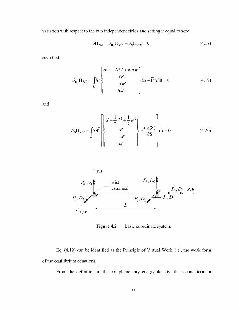
81

variation with respect to the two independent fields and setting it equal to zero

00HR HR HRδ δ δΠ = Π + Π =u S (4.18)

such that

0T Td 0HR

L

u v v w wv

xw

δ δ δδ

δ δδδψ

′ ′ ′ ′ ′+ + ′′ Π = − = ′′− ′

∫u S P D (4.19)

and

2 21 12 2

( ) d 0THR

L

u v w

v xw

χδ δ

ψ

′ ′ ′+ + ∂ ′′Π = − =

∂ ′′− ′

∫SSS

S(4.20)

y v,

x u,

1 1,P D

5 5,P D

2 2,P DL

,z w

6 6,P D

3 3,P D

4 4,P D twist restrained

Figure 4.2 Basic coordinate system.

Eq. (4.19) can be identified as the Principle of Virtual Work, i.e., the weak form

of the equilibrium equations.

From the definition of the complementary energy density, the second term in

82

square brackets in eq. (4.20) corresponds to the section deformations (eq. (4.9)), i.e., the

work conjugate of the stress resultants S

( )χ∂=

∂Sd

S(4.21)

Therefore, substitution of eq. (4.21) into eq. (4.20) gives

2 21 12 2

d 0T

L

u v w

v xw

δ

θ

′ ′ ′+ + ′′ − = ′′−

′

∫ S d (4.22)

Consequently, eq. (4.22) corresponds to the weak form of the compatibility

equation (4.7).

4.4 Equilibrium equations

The equations of equilibrium, consistent with the kinematic hypothesis stated in

Section 4.2, are obtained from eq. (4.19) rewritten here in expanded form

1 1 2 2 3 3 4 4 5 5 6 6

( ) d

0

z yL

N u v v w w M v M w T x

P D P D P D P D P D P D

δ δ δ δ δ δψ

δ δ δ δ δ δ

′ ′ ′ ′ ′ ′′ ′′ ′+ + + − +

− − − − − − =

∫(4.23)

This equation is valid for all kinematically admissible uδ , vδ , wδ and δψ

satisfying the essential boundary conditions (see Figure 4.2)

(0) (0) ( ) (0) ( ) (0) 0u v v L w w Lδ δ δ δ δ δψ= = = = = = (4.24)

Integration of eq. (4.23) by parts, and application of the boundary conditions

83

(4.24) leads to

[ ] [ ] [ ] [ ]

[ ]

0

1 1 2 2 3 3

4 4 5 5 6 6

( ) ( ) d

( ) (0) ( )

(0) ( ) ( ) 0

Lz y

z z

y y

N u Nv M v Nw M w T x

N L P D M P D M L P D

M P D M L P D T L P D

δ δ δ δψ

δ δ δ

δ δ δ

′ ′ ′ ′′ ′ ′ ′′ ′+ − + + +

+ − + + + + − +

+ + + − + + − + =

∫(4.25)

If eq. (4.25) is to be satisfied for all admissible variations, the following equations

of equilibrium (consistent forms of linear and angular momentum balance equations) are

obtained

2

2

2

2

( ) 0

( ) ( )( ) 0

( ) ( )( ) 0

( ) 0

z

y

dN xdx

d M x d dv xN xdx dxdx

d M x d dw xN xdx dxdx

dT xdx

= − + = + =

=

in [0, ]L (4.26)

with the following natural boundary conditions

1 2 3

4 5 6

( ) (0) ( )(0) ( ) ( )

z z

y y

N L P M P M L PM P M L P T L P

= = − == − = =

(4.27)

Since the displacement variation fields are arbitrary in this derivation, the

equilibrium equations are satisfied pointwise (strong form).

From eqs. (4.26) it is observed that the axial force ( )N x and the torsional moment

( )T x are constant along the element. The expressions for the bending moments ( )zM x

and ( )yM x are obtained, respectively, by integrating twice the second and third of

eqs. (4.26). Then, using the natural boundary conditions (4.27), the following stress

resultant fields are obtained:

84

1

1 2 3

1 4 5

6

( )

( ) ( ) 1

( ) ( ) 1

( )

z

z

N x P

x xM x v x P P PL L

x xM x w x P P PL L

T x P

=

= + − + = − + − +

=

(4.28)

This equation can be rewritten in matrix form as a relation between section forces

( )xS and end forces P

( ) ( )x x=S b P (4.29)

where

1 0 0 0 0 0( ) 1 0 0 0

( ) ,( ) 0 0 1 0

0 0 0 0 0 1

v xxw Lξ ξ ξ

ξξ ξ ξ

− = = − −

b (4.30)

is the matrix of displacement-dependent force interpolation functions, with x Lξ =

being the natural coordinate along the element.

4.5 Weak form of the compatibility equation

The compatibility equations are imposed weakly using eq. (4.22), which is repeated here

in expanded form

( ) ( )

( )

2 20

1 12 2

d 0

z z y yL

N u v w M v M w

T x

δ ε δ κ δ κ

δ θ ϕ

′ ′ ′ ′′ ′′+ + − + − + − −

′+ − =

∫ (4.31)

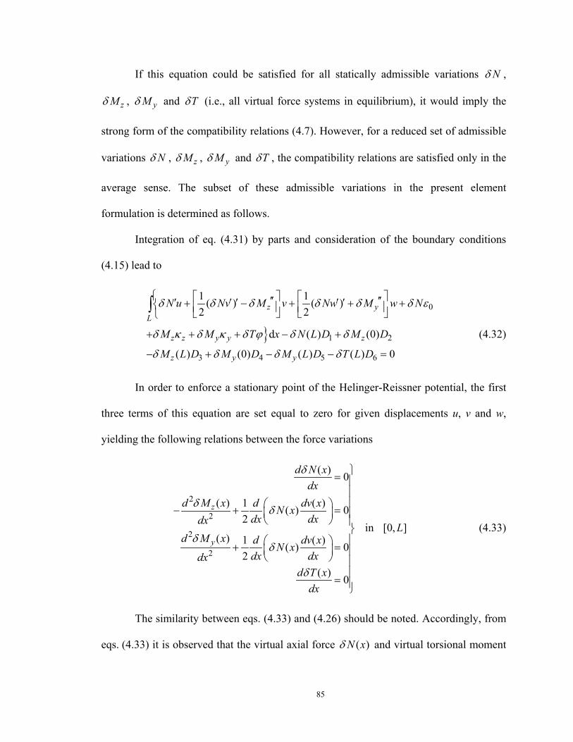
85

If this equation could be satisfied for all statically admissible variations Nδ ,

zMδ , yMδ and Tδ (i.e., all virtual force systems in equilibrium), it would imply the

strong form of the compatibility relations (4.7). However, for a reduced set of admissible

variations Nδ , zMδ , yMδ and Tδ , the compatibility relations are satisfied only in the

average sense. The subset of these admissible variations in the present element

formulation is determined as follows.

Integration of eq. (4.31) by parts and consideration of the boundary conditions

(4.15) lead to

0

1 2

3 4 5 6

1 1( ) ( )2 2

d ( ) (0)

( ) (0) ( ) ( ) 0

z yL

z z y y z

z y y

N u Nv M v Nw M w N

M M T x N L D M D

M L D M D M L D T L D

δ δ δ δ δ δ ε

δ κ δ κ δ ϕ δ δ

δ δ δ δ

′′ ′′′ ′ ′ ′ ′+ − + + +

+ + + − +

− + − − =

∫

(4.32)

In order to enforce a stationary point of the Helinger-Reissner potential, the first

three terms of this equation are set equal to zero for given displacements u, v and w,

yielding the following relations between the force variations

2

2

2

2

( ) 0

( ) 1 ( )( ) 02

( ) 1 ( )( ) 02

( ) 0

z

y

d N xdx

d M x d dv xN xdx dxdx

d M x d dv xN xdx dxdx

d T xdx

δ

δ δ

δδ

δ

= − + = + =

=

in [0, ]L (4.33)

The similarity between eqs. (4.33) and (4.26) should be noted. Accordingly, from

eqs. (4.33) it is observed that the virtual axial force ( )N xδ and virtual torsional moment

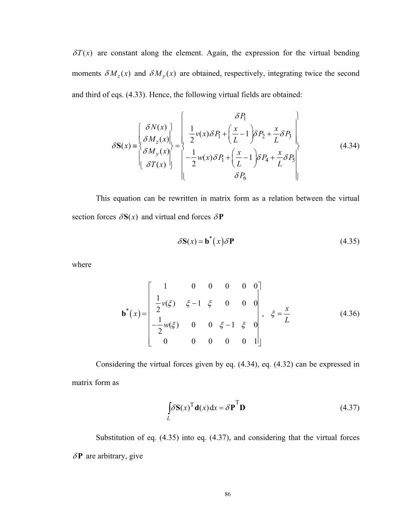
86

( )T xδ are constant along the element. Again, the expression for the virtual bending

moments ( )zM xδ and ( )yM xδ are obtained, respectively, integrating twice the second

and third of eqs. (4.33). Hence, the following virtual fields are obtained:

1

1 2 3

1 4 5

6

( ) 1 ( ) 1( ) 2

( )( ) 1 ( ) 1

2( )

z

y

PN x x xv x P P P

M x L Lx

M x x xw x P P PL LT xP

δδ

δ δ δδ

δδ

δ δ δδ

δ

+ − + ≡ =

− + − +

S (4.34)

This equation can be rewritten in matrix form as a relation between the virtual

section forces ( )xδS and virtual end forces δP

( )*( )x xδ δ=S b P (4.35)

where

( )*

1 0 0 0 0 01 ( ) 1 0 0 02 ,1 ( ) 0 0 1 02

0 0 0 0 0 1

v xxLw

ξ ξ ξξ

ξ ξ ξ

− = = − −

b (4.36)

Considering the virtual forces given by eq. (4.34), eq. (4.32) can be expressed in

matrix form as

TT( ) ( )dL

x x xδ δ=∫ S d P D (4.37)

Substitution of eq. (4.35) into eq. (4.37), and considering that the virtual forces

δP are arbitrary, give

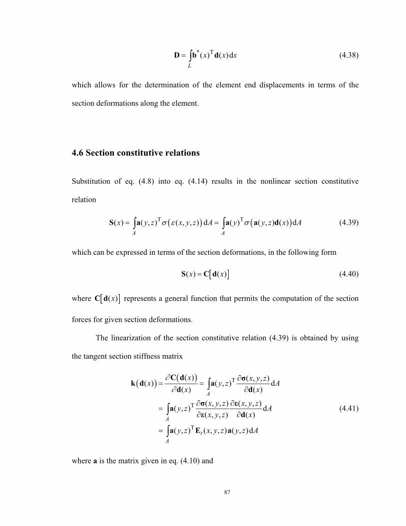
87

* T( ) ( )dL

x x x= ∫D b d (4.38)

which allows for the determination of the element end displacements in terms of the

section deformations along the element.

4.6 Section constitutive relations

Substitution of eq. (4.8) into eq. (4.14) results in the nonlinear section constitutive

relation

( ) ( )T T( ) ( , ) ( , , ) d ( ) ( , ) ( ) dA A

x y z x y z A y y z x Aσ ε σ= =∫ ∫S a a a d (4.39)

which can be expressed in terms of the section deformations, in the following form

[ ]( ) ( )x x=S C d (4.40)

where [ ]( )xC d represents a general function that permits the computation of the section

forces for given section deformations.

The linearization of the section constitutive relation (4.39) is obtained by using

the tangent section stiffness matrix

( ) ( ) T

T

T

( ) ( , , )( ) ( , ) d( ) ( )

( , , ) ( , , )( , ) d( , , ) ( )

( , ) ( , , ) ( , )d

A

A

tA

x x y zx y z Ax x

x y z x y zy z Ax y z x

y z x y z y z A

∂∂

∂= =

∂

∂ ∂=

∂ ∂

=

∫

∫

∫

C d σk d ad d

σ εaε d

a E a

(4.41)

where a is the matrix given in eq. (4.10) and

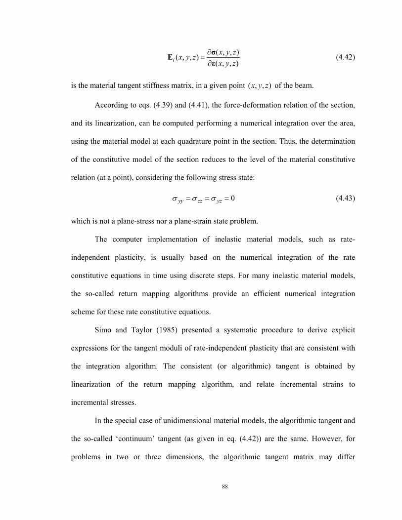
88

( , , )( , , )( , , )tx y zx y zx y z

∂=∂σEε

(4.42)

is the material tangent stiffness matrix, in a given point ( , , )x y z of the beam.

According to eqs. (4.39) and (4.41), the force-deformation relation of the section,

and its linearization, can be computed performing a numerical integration over the area,

using the material model at each quadrature point in the section. Thus, the determination

of the constitutive model of the section reduces to the level of the material constitutive

relation (at a point), considering the following stress state:

0yy zz yzσ σ σ= = = (4.43)

which is not a plane-stress nor a plane-strain state problem.

The computer implementation of inelastic material models, such as rate-

independent plasticity, is usually based on the numerical integration of the rate

constitutive equations in time using discrete steps. For many inelastic material models,

the so-called return mapping algorithms provide an efficient numerical integration

scheme for these rate constitutive equations.

Simo and Taylor (1985) presented a systematic procedure to derive explicit

expressions for the tangent moduli of rate-independent plasticity that are consistent with

the integration algorithm. The consistent (or algorithmic) tangent is obtained by

linearization of the return mapping algorithm, and relate incremental strains to

incremental stresses.

In the special case of unidimensional material models, the algorithmic tangent and

the so-called ‘continuum’ tangent (as given in eq. (4.42)) are the same. However, for

problems in two or three dimensions, the algorithmic tangent matrix may differ

89

considerably from the ‘continuum’ tangent, especially when large time steps are used.

Only when the time steps tend to zero will the consistent and the continuum tangent

moduli coincide.

Therefore, the algorithmic tangent must be used in order to maintain the quadratic

convergence rate of the global solution strategy, usually based on Newton-Raphson

method.

Park and Lee (1996) presented an effective stress update algorithm to integrate

elastoplastic rate equations for a beam element, under the stress state defined in eq.(4.43).

A consistent elastoplastic tangent, for this particular stress state, is given in that paper.

From the consistent elastoplastic tangent of each quadrature point of the section,

the consistent section stiffness matrix can be determined using eq. (4.41) (with the

algorithmic tangent in place of tE )

( ) ( )

0

0

0

0

( ) ( ) ( ) ( )( ) ( ) ( ) ( )

( ) ( ) ( ) ( )( ) ( ) ( ) ( )( )

( )( ) ( ) ( ) ( )( )( ) ( ) ( ) ( )

( ) ( ) ( ) ( )( ) ( ) ( ) ( )

z y

z z z z

z y

y y y y

z y

z y

N x N x N x N xx x x x

M x M x M x M xx x x xx

xM x M x M x M xx

x x x x

T x T x T x T xx x x x

ε κ κ ϕ

ε κ κ ϕ∂∂

ε κ κ ϕ

ε κ κ ϕ

∂ ∂ ∂ ∂∂ ∂ ∂ ∂

∂ ∂ ∂ ∂∂ ∂ ∂ ∂

= =∂ ∂ ∂ ∂

∂ ∂ ∂ ∂

∂ ∂ ∂ ∂∂ ∂ ∂ ∂

C dk d

d

(4.44)

which relates section deformation increments to section force increments.

The section tangent flexibility matrix ( )xf , necessary in the flexibility-based

formulation, is obtained by inverting the section tangent stiffness matrix ( )xk

90

0 0 0 0( ) ( ) ( ) ( )( ) ( ) ( ) ( )

( ) ( ) ( ) ( )( ) ( ) ( ) ( )

( )( ) ( ) ( ) ( )( ) ( ) ( ) ( )

( ) ( ) ( ) ( )( ) ( ) ( ) ( )

z y

z z z z

z y

y y y y

z y

z y

x x x xN x M x M x T x

x x x xN x M x M x T x

xx x x x

N x M x M x T x

x x x xN x M x M x T x

ε ε ε ε

κ κ κ κ

κ κ κ κ

ϕ ϕ ϕ ϕ

∂ ∂ ∂ ∂ ∂ ∂ ∂ ∂ ∂ ∂ ∂ ∂∂ ∂ ∂ ∂

≡ ∂ ∂ ∂ ∂ ∂ ∂ ∂ ∂∂ ∂ ∂ ∂

∂ ∂ ∂ ∂

f -1( )x

=

k (4.45)

4.6.1 Simplified section constitutive relation

A simplified section constitutive relation can be defined based on the assumption of a

uniaxial stress state (in the direction x) at each integration point over the section. The

axial force and bending moment, as well as the corresponding section stiffness terms, can

then be obtained with the traditional fiber section, which is based on the assumption of

uniaxial stress. The torsional behavior is assumed to be uncoupled from the flexural

behavior and governed by a general unidimensional constitutive relation. With these

assumptions, the section constitutive relation is written as

T1 11( , ) ( ( , ) ( ))d

( )( ( ))

xxA

y z y z x Ax

T T x

σ

ϕ

= =

∫a a dSS (4.46)

whereT

1 z yN M M=S (4.47)

and

1 1 0y z= −a (4.48)

The section tangent stiffness is then

91

T1 1d

d ( )d

tA

E A

T ϕϕ

=

∫a a 0

k0

(4.49)

In the elastic range, the term d dT ϕ corresponds to the torsional stiffness JG.

4.7 Consistent flexibility matrix

The flexibility matrix for the geometrically nonlinear flexibility-based element is

obtained by taking the derivative of end displacements D (eq. (4.38)) with respect to end

forces P. The derivation is done using indicial notation.

**

* **

* **

* *

d

d

d

ji jiik j jiLk k k

ji ji j lj j jiL k k l k

ji ji lmj j ji jl lk mL k k k

ji jij

k k

b dDF d b xP P P

b b dv w Sd d b xv P w P S P

b bv w bd d b f b P xv P w P P

b bv wdv P w P

∂ ∂∂ = = +

∂ ∂ ∂ ∂ ∂ ∂∂ ∂ ∂ = + +∂ ∂ ∂ ∂ ∂ ∂

∂ ∂ ∂ ∂ ∂ = + + + ∂ ∂ ∂ ∂ ∂

∂ ∂∂ ∂= +

∂ ∂ ∂ ∂

∫

∫

∫

( )

*

*

d

d

lmj ji jl lk mL k

lmm

k

ik ji jl lk lkL

b vd b f b Pv P

b wP xw P

g b f b h x

∂ ∂ + + ∂ ∂

∂ ∂+ ∂ ∂ = + +

∫

∫

(4.50)

which can be rewritten in the same form as in the planar case, using matrix notation

[ ] * T( ) ( ) ( ) ( ) ( ) dL

x x x x x x∂= = + +∂ ∫DF b f b h gP

(4.51)

92

where

T T

1 2 3 4 5 61

1 2 3 4 5 6

( ) ( ) ( ) ( )( )( ) ( )

0 0 0 0 0 0( ) ( ) ( ) ( ) ( ) ( )

( ) ( ) ( ) ( ) ( ) ( )

0 0 0 0 0 0

x v x x w xxv x w x

v x v x v x v x v x v xP P P P P P

Pw x w x w x w x w x w x

P P P P P P

∂ ∂ ∂ ∂ = + ∂ ∂ ∂ ∂ ∂ ∂ ∂ ∂ ∂ ∂

∂ ∂ ∂ ∂ ∂ ∂ = ∂ ∂ ∂ ∂ ∂ ∂ − − − − − −

∂ ∂ ∂ ∂ ∂ ∂

b bh P PP P

(4.52)

and

T T* T * T

1 2 3 4 5 6

1 2 3 4 5 6

( ) ( ) ( ) ( )( )( ) ( )

0 0 0 0 0 01 0 0 0 0 0 02

0 0 0 0 0 00 0 0 0 0 00 0 0 0 0 0

0 0 0 0 0 01 0 0 0 0 0 02

0 0 0 0 0 0

z

y

x v x x w xxv x w x

v v v v v vP P P P P P

w w w w w wP P P P P P

κ

κ

∂ ∂ ∂ ∂ = + ∂ ∂ ∂ ∂ ∂ ∂ ∂ ∂ ∂ ∂

∂ ∂ ∂ ∂ ∂ ∂ = ∂ ∂ ∂ ∂ ∂ ∂∂ ∂ ∂ ∂ ∂ ∂

−

b bg d dP P

0 0 0 0 0 00 0 0 0 0 0

(4.53)

The terms

1 2 3 4 5 6

1 2 3 4 5 6

( ) ( ) ( ) ( ) ( ) ( ) ( )

( ) ( ) ( ) ( ) ( ) ( ) ( )

v x v x v x v x v x v x v xP P P P P P

w x w x w x w x w x w x w xP P P P P P

∂ ∂ ∂ ∂ ∂ ∂ ∂= ∂ ∂ ∂ ∂ ∂ ∂ ∂ ∂ ∂ ∂ ∂ ∂ ∂ ∂

= ∂ ∂ ∂ ∂ ∂ ∂ ∂

P

P

(4.54)

93

are derived in the following section.

4.8 Curvature-based displacement interpolation (CBDI)

Displacements ( )v x and ( )w x need to be obtained from curvature fields ( )z xκ and

( )y xκ , respectively.

As in the planar case, displacements iv and iw , evaluated at sample points iξ (for

1, ,i n= … ) can be expressed in terms of the curvatures z jκ and y jκ as

* *i ij z i ij yj j

j jv l w lκ κ= = −∑ ∑ (4.55)

for 1, ,i n= … and 1, ,j n= … . Eqs. (4.55) can be written in matrix form as

* *z y= = −v l κ w l κ (4.56)

where

T T1 1n nv v w w= =v w (4.57)

are the transverse displacements at the integration points, and

TT1 1z z z y y yn n

κ κ κ κ= =κ κ (4.58)

are the corresponding curvatures at the integration points. The matrix *l is the same as in

the planar case, and is given by eq. (2.60).

Functions ( )v x∂ ∂ P and ( )w x∂ ∂ P , necessary for the computation of the

flexibility matrix (eq. (4.51)), are evaluated at the integration points, forming the matrices

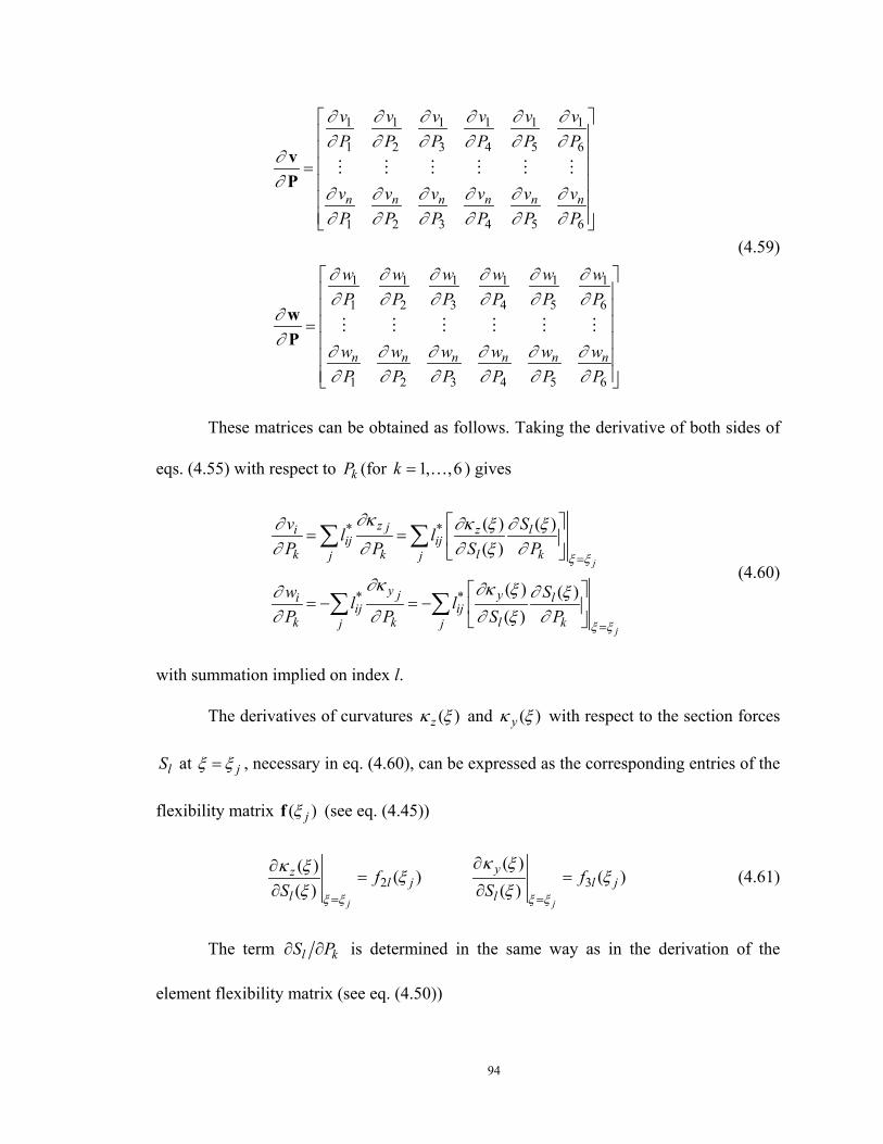
94

1 1 1 1 1 1

1 2 3 4 5 6

1 2 3 4 5 6

1 1 1 1 1 1

1 2 3 4 5 6

1 2 3 4 5 6

n n n n n n

n n n n n n

v v v v v vP P P P P P

v v v v v vP P P P P P

w w w w w wP P P P P P

w w w w w wP P P P P P

∂ ∂ ∂ ∂ ∂ ∂∂ ∂ ∂ ∂ ∂ ∂

∂∂

∂ ∂ ∂ ∂ ∂ ∂∂ ∂ ∂ ∂ ∂ ∂

∂ ∂ ∂ ∂ ∂ ∂∂ ∂ ∂ ∂ ∂ ∂

∂∂

∂ ∂ ∂ ∂ ∂ ∂∂ ∂ ∂ ∂ ∂ ∂

=

=

vP

wP

(4.59)

These matrices can be obtained as follows. Taking the derivative of both sides of

eqs. (4.55) with respect to kP (for 1, ,6k = … ) gives

* *

* *

( ) ( )( )

( ) ( )( )

j

j

z ji z lij ij

k k l kj j

y j yi lij ij

k k l kj j

v Sl lP P S P

w Sl lP P S P

ξ ξ

ξ ξ

∂κ∂ ∂κ ξ ∂ ξ∂ ∂ ∂ ξ ∂

∂κ ∂κ ξ∂ ∂ ξ∂ ∂ ∂ ξ ∂

=

=

= =

= − = −

∑ ∑

∑ ∑(4.60)

with summation implied on index l.

The derivatives of curvatures ( )zκ ξ and ( )yκ ξ with respect to the section forces

lS at jξ ξ= , necessary in eq. (4.60), can be expressed as the corresponding entries of the

flexibility matrix ( )jξf (see eq. (4.45))

2 3( )( ) ( ) ( )

( ) ( )j j

yzl j l j

l lf f

S Sξ ξ ξ ξ

κ ξκ ξ ξ ξξ ξ= =

∂∂= =

∂ ∂(4.61)

The term l kS P∂ ∂ is determined in the same way as in the derivation of the

element flexibility matrix (see eq. (4.50))

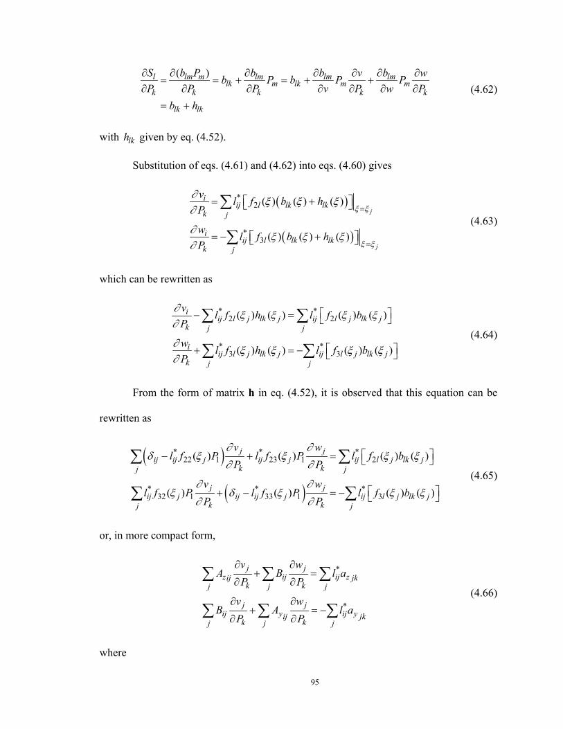
95

( )l lm m lm lm lmlk m lk m m

k k k k k

lk lk

S b P b b v b wb P b P PP P P v P w P

b h

∂ ∂ ∂ ∂ ∂ ∂ ∂= = + = + +

∂ ∂ ∂ ∂ ∂ ∂ ∂= +

(4.62)

with lkh given by eq. (4.52).

Substitution of eqs. (4.61) and (4.62) into eqs. (4.60) gives

( )

( )

*2

*3

( ) ( ) ( )

( ) ( ) ( )

j

j

iij l lk lk

k j

iij l lk lk

k j

v l f b hP

w l f b hP

ξ ξ

ξ ξ

∂ ξ ξ ξ∂

∂ ξ ξ ξ∂

=

=

= +

= − +

∑

∑(4.63)

which can be rewritten as

* *2 2

* *3 3

( ) ( ) ( ) ( )

( ) ( ) ( ) ( )

iij l j lk j ij l j lk j

k j j

iij l j lk j ij l j lk j

k j j

v l f h l f bP

w l f h l f bP

∂ ξ ξ ξ ξ∂

∂ ξ ξ ξ ξ∂

− =

+ = −

∑ ∑

∑ ∑(4.64)

From the form of matrix h in eq. (4.52), it is observed that this equation can be

rewritten as

( )

( )

* * *22 1 23 1 2

* * *32 1 33 1 3

( ) ( ) ( ) ( )

( ) ( ) ( ) ( )

j jij ij j ij j ij l j lk j

k kj j

j jij j ij ij j ij l j lk j

k kj j

v wl f P l f P l f b

P P

v wl f P l f P l f b

P P

∂ ∂δ ξ ξ ξ ξ

∂ ∂

∂ ∂ξ δ ξ ξ ξ

∂ ∂

− + =

+ − = −

∑ ∑

∑ ∑(4.65)

or, in more compact form,

*

*

j jz ij ij zij jk

k kj j j

j jij y ij yij jk

k kj j j

v wA B l a

P P

v wB A l a

P P

∂ ∂+ =

∂ ∂

∂ ∂+ = −

∂ ∂

∑ ∑ ∑

∑ ∑ ∑(4.66)

where

96

*22 1

*33 1

*23 1

2

3

( )

( )

( )

( ) ( )

( ) ( )

z ij ij jij

y ij ij jij

ij ij j

z l j lk jjkl

y l j lk jjkl

A l f P

A l f P

B l f P

a f b

a f b

δ ξ

δ ξ

ξ

ξ ξ

ξ ξ

= −

= −

=

=

=

∑

∑

(4.67)

Rewriting eq. (4.66) in matrix notation, and solving for the terms ∂ ∂v P and

∂ ∂w P , defined in eq. (4.59), gives

1 *

*z z

y y

−∂

∂ = ∂ − ∂

vA B l aPB Aw l a

P

(4.68)

Clearly, instead of computing the matrix inverse, it is more efficient to solve the

corresponding system of equations.

4.9 Corotational formulation

The transformation between the basic and global systems is done according to the

corotational formulation. In the planar case described in Chapter 3, this transformation is

exact, with no assumption being made on the size of the local displacements (except to

avoid singularities for rigid body rotations with norm larger than 180 degrees). In three-

dimensions, however, different formulations were proposed based on different definitions

of the basic system, and on different assumptions related to the size of the basic rotations.

Although several of the procedures proposed in the literature could be used with

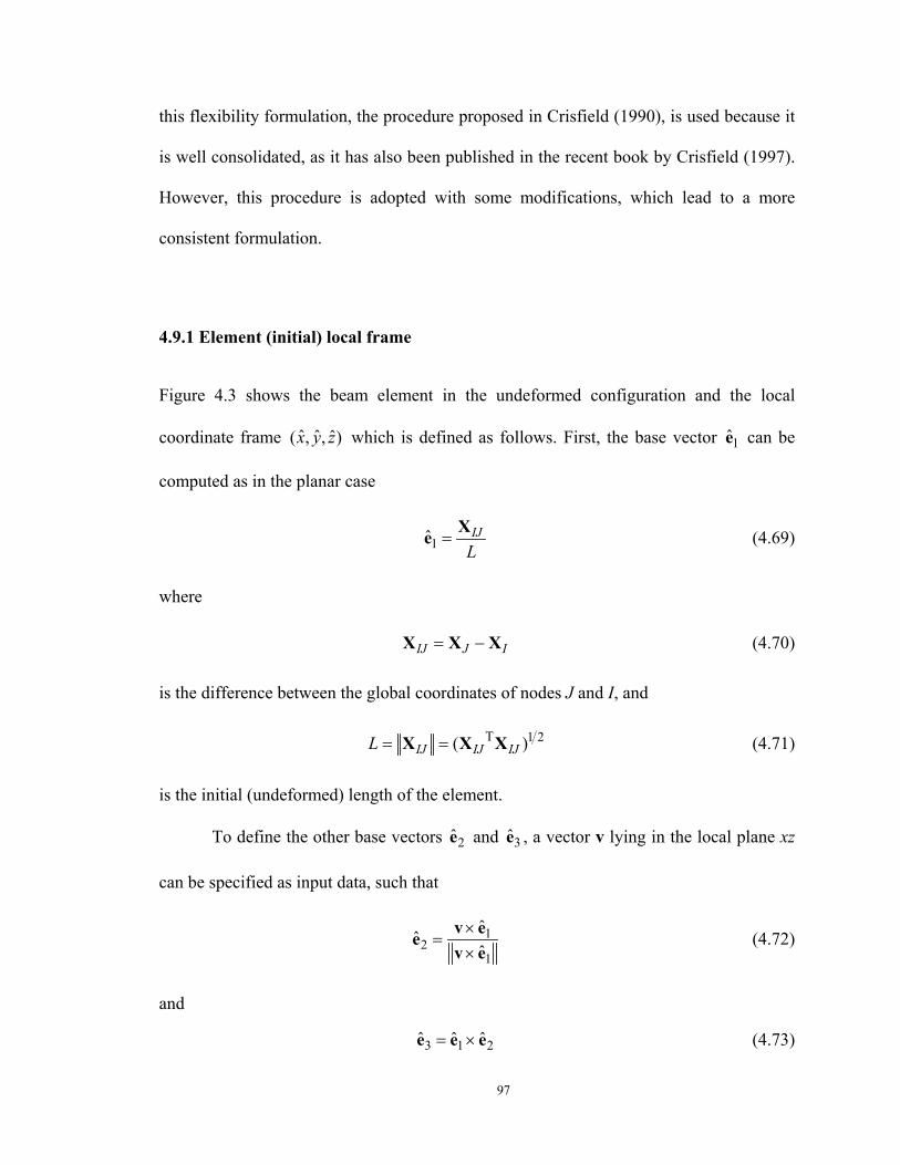
97

this flexibility formulation, the procedure proposed in Crisfield (1990), is used because it

is well consolidated, as it has also been published in the recent book by Crisfield (1997).

However, this procedure is adopted with some modifications, which lead to a more

consistent formulation.

4.9.1 Element (initial) local frame

Figure 4.3 shows the beam element in the undeformed configuration and the local

coordinate frame ˆ ˆ ˆ( , , )x y z which is defined as follows. First, the base vector 1e can be

computed as in the planar case

1ˆ IJL

=Xe (4.69)

where

IJ J I= −X X X (4.70)

is the difference between the global coordinates of nodes J and I, and

T 1 2( )IJ IJ IJL = =X X X (4.71)

is the initial (undeformed) length of the element.

To define the other base vectors 2e and 3e , a vector v lying in the local plane xz

can be specified as input data, such that

12

1

ˆˆˆ

×=

×v eev e

(4.72)

and

3 1 2ˆ ˆ ˆ= ×e e e (4.73)

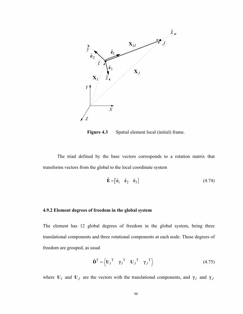
98

IJX

x

J

I

IXJX

y2e 1e

3e

z

X

Y

Z

Figure 4.3 Spatial element local (initial) frame.

The triad defined by the base vectors corresponds to a rotation matrix that

transforms vectors from the global to the local coordinate system

[ ]1 2 3ˆ ˆ ˆ ˆ=E e e e (4.74)

4.9.2 Element degrees of freedom in the global system

The element has 12 global degrees of freedom in the global system, being three

translational components and three rotational components at each node. These degrees of

freedom are grouped, as usual

T T T TTˆI I J J=D U γ U γ (4.75)

where IU and JU are the vectors with the translational components, and Iγ and Jγ

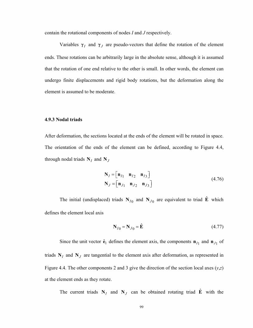
99

contain the rotational components of nodes I and J respectively.

Variables Iγ and Jγ are pseudo-vectors that define the rotation of the element

ends. These rotations can be arbitrarily large in the absolute sense, although it is assumed

that the rotation of one end relative to the other is small. In other words, the element can

undergo finite displacements and rigid body rotations, but the deformation along the

element is assumed to be moderate.

4.9.3 Nodal triads

After deformation, the sections located at the ends of the element will be rotated in space.

The orientation of the ends of the element can be defined, according to Figure 4.4,

through nodal triads IN and JN

1 2 3

1 2 3

I I I I

J J J J

= =

N n n n

N n n n(4.76)

The initial (undisplaced) triads 0IN and 0JN are equivalent to triad E which

defines the element local axis

0 0ˆ

I J= =N N E (4.77)

Since the unit vector 1e defines the element axis, the components 1In and 1Jn of

triads IN and JN are tangential to the element axis after deformation, as represented in

Figure 4.4. The other components 2 and 3 give the direction of the section local axes (y,z)

at the element ends as they rotate.

The current triads IN and JN can be obtained rotating triad E with the

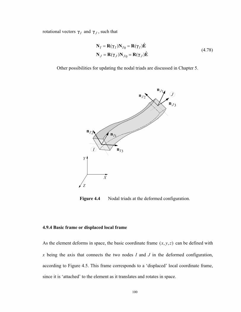
100

rotational vectors Iγ and Jγ , such that

0

0

ˆ( ) ( )ˆ( ) ( )

I I I I

J J J J

= =

= =

N R γ N R γ E

N R γ N R γ E(4.78)

Other possibilities for updating the nodal triads are discussed in Chapter 5.

1In

X

Y

Z

J

I

2In

3In

1Jn2Jn

3Jn

Figure 4.4 Nodal triads at the deformed configuration.

4.9.4 Basic frame or displaced local frame

As the element deforms in space, the basic coordinate frame ( , , )x y z can be defined with

x being the axis that connects the two nodes I and J in the deformed configuration,

according to Figure 4.5. This frame corresponds to a ‘displaced’ local coordinate frame,

since it is ‘attached’ to the element as it translates and rotates in space.

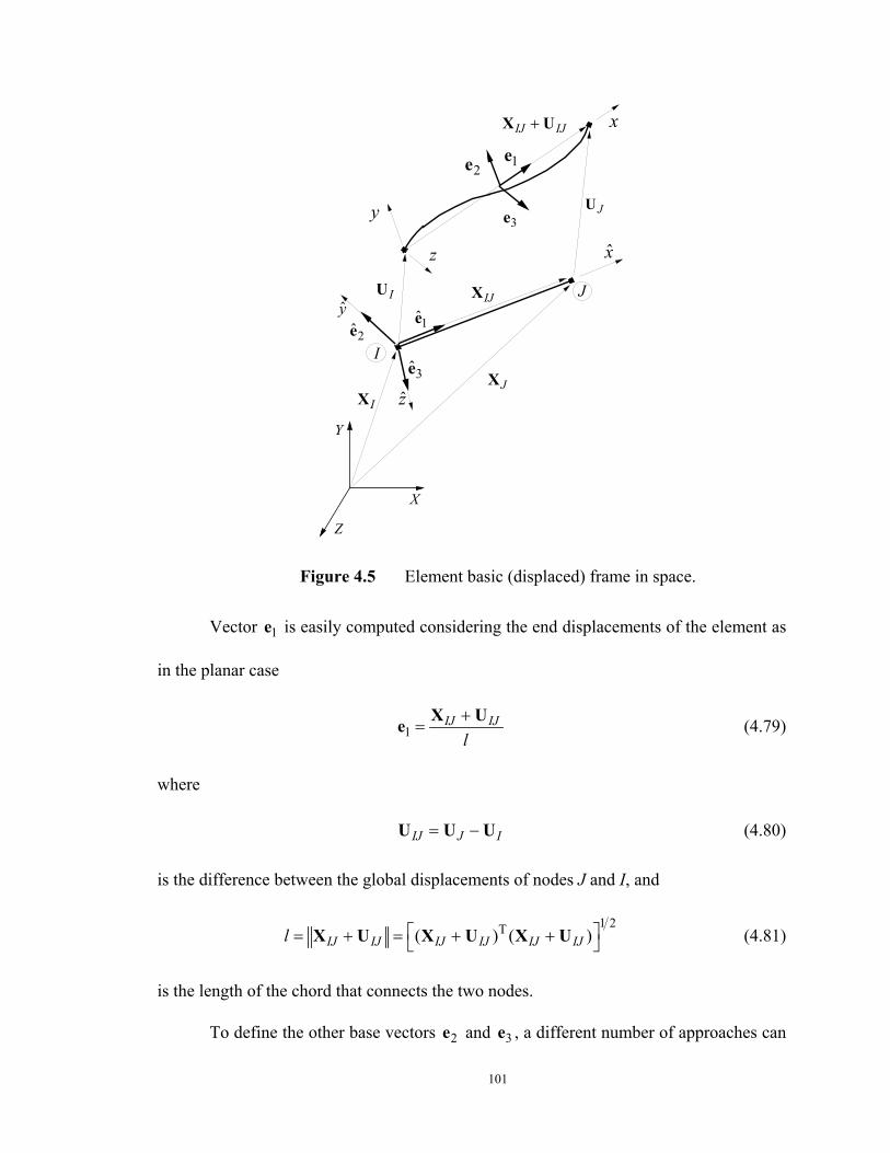
101

x

y

x

IU

JU

IJ IJ+X U

1e2e

IJX J

I

IXJX

y2e 1e

3e

z

X

Y

Z

3e

z

Figure 4.5 Element basic (displaced) frame in space.

Vector 1e is easily computed considering the end displacements of the element as

in the planar case

1IJ IJ

l+

=X Ue (4.79)

where

IJ J I= −U U U (4.80)

is the difference between the global displacements of nodes J and I, and

1 2T( ) ( )IJ IJ IJ IJ IJ IJl = + = + + X U X U X U (4.81)

is the length of the chord that connects the two nodes.

To define the other base vectors 2e and 3e , a different number of approaches can

102

be used (see for example, Rankin and Brogan (1984), Nour-Omid and Rankin (1991), and

Crisfield and Moita (1996)). This definition is not unique because there are several

systems free of rigid body modes that can be adopted. However, the most effective choice

would be the one that minimizes the element displacements with respect to the basic

frame. In addition, it is important to adopt a basic system that is invariant with respect to

node numbering and the definition of the initial local axes y and z (i.e., if the node

numbers I and J, or the local axes y and z , are switched in the input data, the results

should remain the same.)

To compute the other base vectors 2e and 3e , Crisfield (1990) introduces a

rotation matrix R , denominated ‘average nodal rotation matrix’ (or ‘mean rotation

matrix’). This matrix corresponds to an intermediate rotation between triads IN and JN ,

and can be defined in different ways, since it is just used as a reference.

Crisfield (1990) first suggests that this average rotation matrix can be defined as

2I J+ =

γ γR R (4.82)

an expression that is also used in Pacoste and Eriksson (1997). However, Crisfield states,

without justification, that there is a better definition for this matrix, which is described as

follows. First, a rotation matrix ( )R γ , corresponding to the rotation from triad IN to

triad JN , is defined using the compound rotation formula

( )J I=N R γ N (4.83)

Multiplying both sides of this equation by TIN and considering the fact that IN

is an orthogonal matrix gives

103

T( ) J I=R γ N N (4.84)

where γ is the rotation vector associated with this rotation. Crisfield then uses this

rotation vector to define the mean rotation matrix as

2 I =

γR R N (4.85)

arguing that, although the rotation vectors are not additive, γ is assumed to be

moderately large and hence ( 2)R γ can be used as a reasonable representation of the

rotation from IN to the average or mean configuration. To compute the term 2γ ,

Crisfield uses a lengthy procedure, involving the extraction of the unit quaternion from

the rotation matrix ( )R γ , and the use of the tangent scaled and unscaled form of the

rotational vector (see Figure 3.2, and eqs. (3.30) and (3.66)).

Apparently, the motivation for Crisfield to seek an alternative to eq. (4.82) lies in

the fact that this equation requires the explicit computation of the pseudo-vectors Iγ and

Jγ , which can only be done uniquely for angles in the range ( , )π π− .

However, apart from this limitation, the advantage of eq. (4.82) resides in its

simplicity. As will be shown later, the variation of the rotation matrix given by eq. (4.82)

is very straightforward, and can be computed exactly without any simplification.

On the other hand, the variation of the mean rotation matrix as given by eq. (4.85)

is rather complicated. Thus, although Crisfield computes the mean rotation matrix using

eq. (4.85), he computes the variation of the rotation matrix using the simpler variation of

eq. (4.82). Crisfield (1997) justifies this approximation by neglecting higher-order terms

of the correct variation of eq. (4.85), based on the assumption that the relative rotations

104

are small.

For consistency, eq. (4.82) is adopted in the present work to compute the mean

rotation matrix and its corresponding variation.

The mean triad 1 2 3 = R r r r , which corresponds to an intermediate rotation

of the two ends, is an appropriate reference frame to represent the rigid body rotation of

the element as a whole. In particular, the position of unit vectors 2r and 3r can be used

as a reference to measure the twist of the sections along the element. However, vector 1r

does not coincide with the deformed local x axis of the element which connects the two

nodes, i.e., 1r is in general not parallel to base vector 1e .

In order to define triad E, triad R can be rotated such that its unit vector 1r

becomes aligned with the unit vector 1e . This can be easily accomplished by using eqs.

(3.77) and (3.78), such that

T2 1

2 2 1 1T1 1

( )1

= − ++

r ee r r e

r e(4.86)

T3 1

3 3 1 1T1 1

( )1

= − ++

r ee r r e

r e(4.87)

However, the presence of terms in the denominator of the right hand side of these

equations leads to complicated relations for the transformation of forces between the two

coordinate systems, and consequently for the associated geometric stiffness matrix.

Equations (4.86) and (4.87) were derived exactly considering that the rotation

involved in the transformation between the two triads may be arbitrarily large. Assuming

that this rotation is small, 1r would be close to 1e , so Crisfield suggests that these

105

equations can be approximated by the following relations

T2 1

2 2 1 1( )2

= − +r e

e r r e (4.88)

T3 1

3 3 1 1( )2

= − +r e

e r r e (4.89)

The main disadvantage of this simplification is that these vectors form a triad

[ ]1 2 3=E e e e that is not exactly orthogonal. However, Crisfield (1990) claims that

the error is small and that for moderately relative rotations, this lack of orthogonality can

be neglected.

4.9.5 Rotation vectors expressed with respect to the basic frame

Given the triad E , there exists two rotation matrix IR and JR that rotates this triad into

triads IN and JN , such that

I I

J J

==

N R EN R E

(4.90)

Multiplying both sides of eqs. (4.90) by TE , and assuming that E is a orthogonal

matrix, gives

I I

J J

=

=

T

T

R N E

R N E(4.91)

The components of matrices IR and JR refer to the global frame ( , , )X Y Z .

These rotation matrices can be expressed with respect to the basic frame ( , , )x y z , i.e.,

using the basis 1 2 3( , , )e e e , as

106

T T T

T T T

( ) ( )

( ) ( )I I I

J J J

= =

= =

R θ E N E E E N

R θ E N E E E N(4.92)

with Iθ and Jθ being the rotation vectors expressed in the basic frame (as the rotation

matrices are expressed in this frame, according to the last transformation above).

To obtain the rotation vectors Iθ and Jθ , from the rotation matrices

T( )I I=R θ E N and T( )J J=R θ E N , eq. (3.41) could be used. This would, however, lead

to complex variations of the basic rotations.

Crisfield (1997) proposes the use of eq. (3.40) to compute the basic rotations,

such that (see eq. (4.92))

T T3 22 3

T T1 33 1

T T2 11 2

sin 1sin2

I II

I I I I II

I I

θθθ

− = = −

−

e n e n

t θ e n e n

e n e n

(4.93)

where It is the unit vector parallel to rotational vector Iθ , such that I I Iθ=θ t . Crisfield

then simplifies eq. (4.93) by stating that

T T3 22 31

T T1 32 3 1

T T3 2 11 2

sin1sin sin2

sin

I II

I I I I I

I I I

θθ θ

θ

− = = −

−

e n e n

t e n e n

e n e n

(4.94)

which is, in fact, an approximation, since

1

12

2

33

1

2

3

sinsinsin

sin sin sin sinsin sin

sin

II

III I

II I I I I I

II I I

II

I

ttt

θθ

θ θθθ

θ θ θ θθ

θ θθθ

θ

= = ≠

t (4.95)

107

The justification for the use of eq. (4.94) lies in the hypothesis of small basic

rotations. In Crisfield (1990) it is even suggested that the sine function can be

approximated by the angle itself with little loss of accuracy, such that

sin II I

I

θθ

≅θ θ (4.96)

This simplification would be consistent with the level of approximation usually

assumed in the formulation of the element in the basic system, when the end rotations of

the element are approximated by their respective slopes (see eqs. (4.16) and (4.17)).

Apparently, the motivation for the adoption of eq. (4.94) by Crisfield is that for

the particular case of planar problems, this equation reduces to an exact expression. This

is important, since in the planar corotational formulation, exact transformations are

obtained, without the need of simplifying assumptions related to the basic rotations.

4.9.6 Transformation of displacements between coordinate systems

As in the planar case, the axial displacement (with reference to the basic system) is the

difference between the deformed and the initial length

1D u l L≡ = − (4.97)

As discussed before, in the small deformation range, eq. (4.97) is poorly

conditioned, so it is better to express 1D as

T1

1 (2 )IJ IJ IJDl L

= ++

X U U (4.98)

The rotational degrees of freedom are obtained from the components of vectors

108

Iθ and Jθ , which are computed with eq. (4.94) for Iθ , and a similar expression for Jθ

( )( )( )( )( )( )

T T3 21 2 3

T T1 32 3 1

T T2 13 1 2

T T3 21 2 3

T T1 32 3 1

T T2 13 1 2

1arcsin21arcsin21arcsin21arcsin21arcsin21arcsin2

I I I

I I I

I I I

J J J

J J J

J J J

θ

θ

θ

θ

θ

θ

= − = − = − = − = − = −

e n e n

e n e n

e n e n

e n e n

e n e n

e n e n

(4.99)

Crisfield (1990) defines the ‘local displacements’ (which in the present context

have been referred to as basic displacements) as being the seven degrees of freedom

formed by the axial displacements u, given in eq. (4.97), and these six components of Iθ

and Jθ defined in eq. (4.99). Clearly, this definition of basic system has one rigid body

mode, which is the rotation around the x-axis.

However, in the force formulation the basic system must be free of rigid body

modes, such that there is a flexibility matrix associated with it. Thus, in the present work,

the basic displacements are defined, according to Figure 4.1, as (see eq. (4.1))

2 33 3

4 52 2

6 11

I I J Jz z

I I J Jy y

J J I

D DD D

D

θ θ θ θ

θ θ θ θ

ψ θ θ

≡ = ≡ =

≡ = ≡ =

≡ = −

(4.100)

109

4.9.7 Transformation of forces

As discussed for the planar case, a tangential relation between the displacements in the

local and global system is given by

ˆδ δ=D T D (4.101)

where

ˆ∂

=∂DTD

(4.102)

is a transformation matrix.

According to the principle of virtual displacements, this matrix transpose

transforms forces from the basic to the global system, such that

Tˆ =P T P (4.103)

In order to compute matrix T, the variations of the triads that define the basic

displacements, such as IδN , JδN ,δR , and δE , in conjunction with other variables,

such as lδ , need to be computed.

Matrices IδN and JδN are obtained by taking the variation of eqs. (4.78),

according to eq. (3.69), such that

ˆ ˆ( ) ( ) ( ) ( )ˆ ˆ( ) ( ) ( ) ( )

I I I I I I

J J J J J J

δ δ δ δ

δ δ δ δ

= = =

= = =

N R γ E S γ R γ E S γ N

N R γ E S γ R γ E S γ N(4.104)

Thus, the columns of IδN and JδN can be expressed as

( ) ( )( ) ( )

I I I I Ik k k

J J J J Jk k k

δ δ δδ δ δ

= = −

= = −

n S γ n S n γn S γ n S n γ

(4.105)

Similarly, the columns of δR are obtained by taking the variation of eq. (4.82)

110

and using eq. (3.69), such that

( )2 2

I J I Jk k k

δ δ δ δδ + + = = −

γ γ γ γr S r S r (4.106)

Here it is important to appreciate the fact that this variation is computed exactly.

As discussed before, although Crisfield (1990) uses eqs. (4.84) and (4.85) to compute the

mean rotation triad, its variation is assumed to be given by eq. (4.106).

The variation of the deformed length l is obtained, as in the planar case, by

computing the differential of eq. (4.81) and using eq. (4.79)

1 2T T

T

T1

1 ( ) ( ) 2( )21( )

IJ IJ IJ IJ IJ IJ IJ

IJ IJ IJ

IJ

l

l

δ δ

δ

δ

− = + + +

= +

=

X U X U X U U

X U U

e U

(4.107)

The variation of vector 1e is obtained by taking the differential of eq. (4.79) and

making use of eq. (4.107)

T1 1 12

1 1 1( ) IJIJ IJ IJ IJ

IJ

ll l ll

δδ δ δ δ

δ

= − + = −

=

Ue U X U e e U

A U(4.108)

where

T1 1

1( )l

= −A I e e (4.109)

is a symmetric matrix.

The terms 2δe and 3δe are determined taking the differential of eqs. (4.88) and

(4.89), and using eqs. (4.106) and (4.108)

111

T T T1 1 1 1 1 1 1

T T1 1 1 1 1

T T1 1 1

T

1 1( )( ) ( )2 2

1 1 1( ) ( ) ( ) ( ) ( )2 4 41 1( ) ( )2 2

ˆ( )

k k k k k

k k k I J

k k J I

k

δ δ δ δ δ δ

δ δ

δ δ

δ

= − + + − +

= − + + + + + − + − −

=

e r r e r e e r r e e r

S r e r e S r r e S r γ γ

e r r A r e A U U

L r D

(4.110)

for 1,2k = , and where

T T T T T1 2 1 2( ) [ ( ) ( ) ( ) ( ) ]k k k k k= −L r L r L r L r L r (4.111)

with

T T1 1 1 1

T T2 1 1 1 1 1

1 1( ) ( )2 21 1 1( ) ( ) ( ) ( ) ( )2 4 4

k k k

k k k k

= + +

= − − +

L r r e A Ar e r

L r S r r e S r S r e e r(4.112)

The force transformation matrix T is derived next. First, for simplicity, the 6×12

matrix T is partitioned into row-vectors rt with ( 1, ,6r = … ) such that

T T T T T TT1 2 3 4 5 6 = T t t t t t t (4.113)

The first row of matrix T, the row-vector 1t , is computed easily by taking the

differential of eq. (4.97), and using eqs. (4.107)

T T1 1 1

1

( )ˆ

IJ J ID lδ δ δ δ δ

δ

= = = −

=

e U e U U

t D(4.114)

where

T TT T1 1 1 = − t e 0 e 0 (4.115)

For the computation of the remaining rows of transformation matrix T, it is

112

necessary to obtain the variations of Iθ and Jθ .

The component 1Iδθ is obtained by taking the variation of the first of eqs. (4.99)

and using eqs. (4.105) and (4.110)

( )

()

T T T T3 2 3 21 2 3 2 3

1

T T TT T3 2 32 3 2

1T

2 3

T3 22 3 1

1

12cos

1 ˆ ˆ( ) ( ) ( )2cos

( )

1 ˆ( ) ( )2cos

I I I I II

I I I II

I I

I I II

δθ δ δ δ δθ

δ δ δθ

δ

δθ

= − + −

= − −

+

= − +

n e n e e n e n

n L r D n L r D e S n γ

e S n γ

L r n L r n h D

(4.116)

where

( )TT T T T3 21 2 3( ) ( )I I I

= − h 0 S n e S n e 0 0 (4.117)

The variation of 2Iθ is obtained from the second of eqs. (4.99), and considering

eqs. (4.105), (4.108) and (4.110)

( )

()

T T T T1 3 1 32 3 1 3 1

2

T T T33 1

2T T

1 33 1

T3 1 2

2

12cos

1 ˆ( )2cos

( ) ( )

1 ˆ( )2cos

I I I I II

I IJ II

I I I I

I II

δθ δ δ δ δθ

δ δθ

δ δ

δθ

= − + −

= −

− +

= − −

n e n e e n e n

n A U n L r D

e S n γ e S n γ

L r n h D

(4.118)

where

( ) ( ) ( )T T TT T3 12 3 1 3 3( ) ( )I I I I I

= − − h An S n e S n e An 0 (4.119)

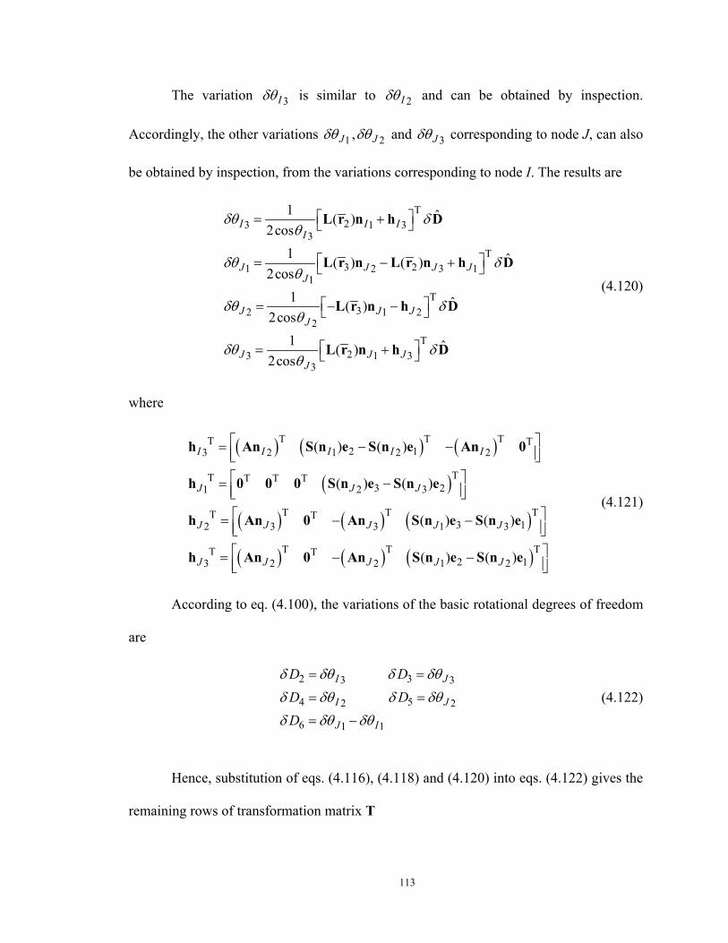
113

The variation 3Iδθ is similar to 2Iδθ and can be obtained by inspection.

Accordingly, the other variations 1Jδθ , 2Jδθ and 3Jδθ corresponding to node J, can also

be obtained by inspection, from the variations corresponding to node I. The results are

T23 1 3

3T

3 21 2 3 11

T32 1 2

2T

23 1 33

1 ˆ( )2cos

1 ˆ( ) ( )2cos

1 ˆ( )2cos

1 ˆ( )2cos

I I II

J J J JJ

J J JJ

J J JJ

δθ δθ

δθ δθ

δθ δθ

δθ δθ

= +

= − +

= − −

= +

L r n h D

L r n L r n h D

L r n h D

L r n h D

(4.120)

where

( ) ( ) ( )

( )

( ) ( ) ( )

( ) ( ) ( )

T T TT T2 13 2 1 2 2

TT T T T3 21 2 3

T T TT T3 12 3 3 1 3

T T TT T2 13 2 2 1 2

( ) ( )

( ) ( )

( ) ( )

( ) ( )

I I I I I

J J J

J J J J J

J J J J J

= − − = − = − − = − −

h An S n e S n e An 0

h 0 0 0 S n e S n e

h An 0 An S n e S n e

h An 0 An S n e S n e

(4.121)

According to eq. (4.100), the variations of the basic rotational degrees of freedom

are

2 33 3

4 52 2

6 11

I J

I J

J I

D DD DD

δ δθ δ δθ

δ δθ δ δθδ δθ δθ

= =

= =

= −

(4.122)

Hence, substitution of eqs. (4.116), (4.118) and (4.120) into eqs. (4.122) gives the

remaining rows of transformation matrix T

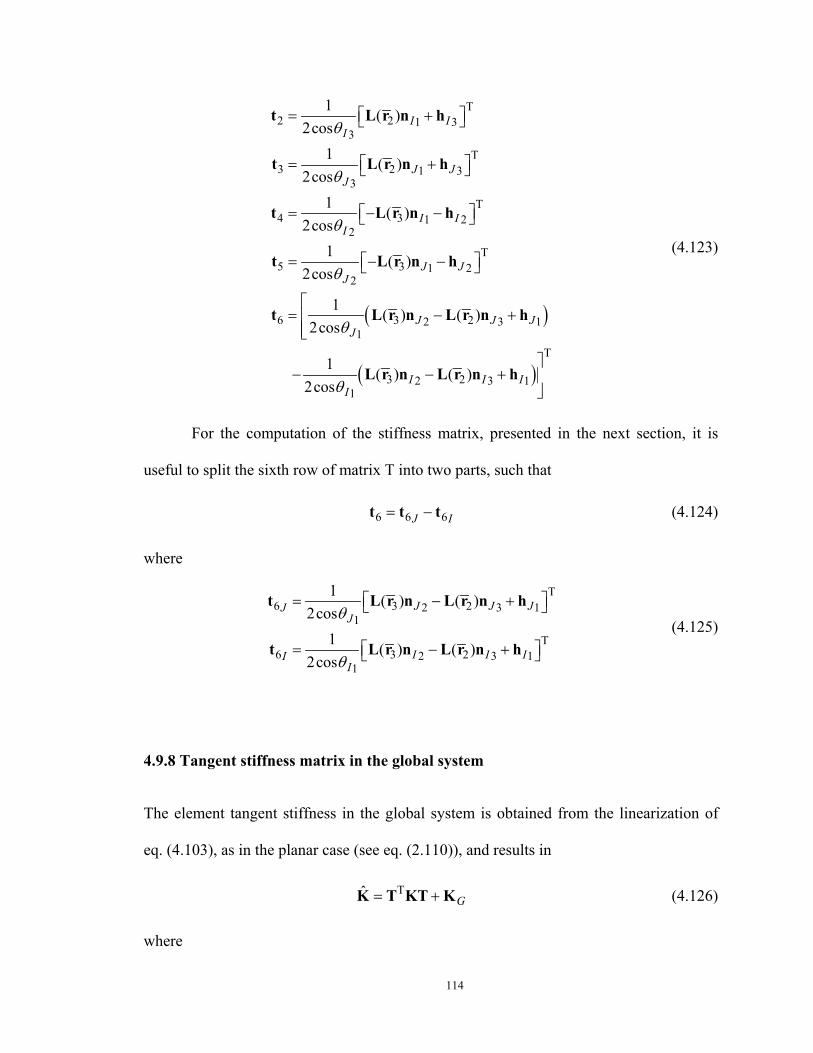
114

( )

( )

T2 2 1 3

3

T3 2 1 3

3

T4 3 1 2

2

T5 3 1 2

2

6 3 22 3 11

T

3 22 3 11

1 ( )2cos

1 ( )2cos

1 ( )2cos

1 ( )2cos

1 ( ) ( )2cos

1 ( ) ( )2cos

I II

J JJ

I II

J JJ

J J JJ

I I II

θ

θ

θ

θ

θ

θ

= +

= +

= − −

= − −

= − +

− − +

t L r n h

t L r n h

t L r n h

t L r n h

t L r n L r n h

L r n L r n h

(4.123)

For the computation of the stiffness matrix, presented in the next section, it is

useful to split the sixth row of matrix T into two parts, such that

6 6 6J I= −t t t (4.124)

where

T6 3 22 3 1

1

T6 3 22 3 1

1

1 ( ) ( )2cos

1 ( ) ( )2cos

J J JJJ

I I III

θ

θ

= − +

= − +

t L r n L r n h

t L r n L r n h(4.125)

4.9.8 Tangent stiffness matrix in the global system

The element tangent stiffness in the global system is obtained from the linearization of

eq. (4.103), as in the planar case (see eq. (2.110)), and results in

TˆG= +K T KT K (4.126)

where

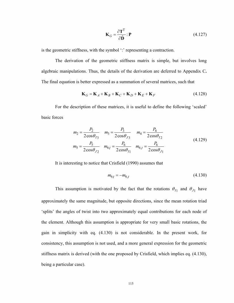
115

T:ˆG

∂=

∂TK PD

(4.127)

is the geometric stiffness, with the symbol ‘:’ representing a contraction.

The derivation of the geometric stiffness matrix is simple, but involves long

algebraic manipulations. Thus, the details of the derivation are deferred to Appendix C.

The final equation is better expressed as a summation of several matrices, such that

G A B C D E F= + + + + +K K K K K K K (4.128)

For the description of these matrices, it is useful to define the following ‘scaled’

basic forces

2 3 42 3 4

3 23

5 6 65 6 6

12 1

2cos 2cos 2cos

2cos 2cos 2cos

I J I

I JJ I J

P P Pm m m

P P Pm m m

θ θ θ

θ θ θ

= = =

= = =(4.129)

It is interesting to notice that Crisfield (1990) assumes that

6 6I Jm m= − (4.130)

This assumption is motivated by the fact that the rotations 1Iθ and 1Jθ have

approximately the same magnitude, but opposite directions, since the mean rotation triad

‘splits’ the angles of twist into two approximately equal contributions for each node of

the element. Although this assumption is appropriate for very small basic rotations, the

gain in simplicity with eq. (4.130) is not considerable. In the present work, for

consistency, this assumption is not used, and a more general expression for the geometric

stiffness matrix is derived (with the one proposed by Crisfield, which implies eq. (4.130),

being a particular case).

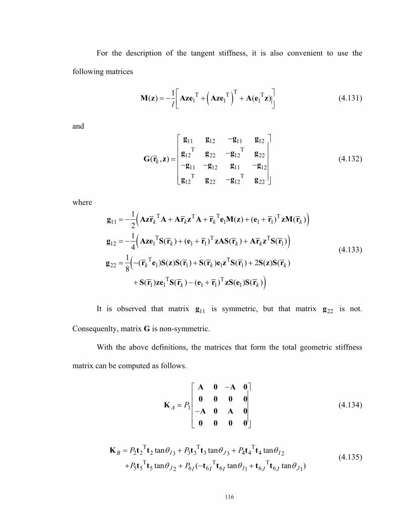
116

For the description of the tangent stiffness, it is also convenient to use the

following matrices

( )TT T T1 1 1

1( ) ( )l = − + +

M z Aze Aze A e z (4.131)

and

11 12 11 12T T

12 22 12 22

11 12 11 12T T

12 22 12 22

( , )k

−

− = − − − −

g g g g

g g g gG r z

g g g g

g g g g

(4.132)

where

( )( )

()

T TT T11 1 1 1

T T T12 1 1 1 1

T T22 1 1 1 1

T T1 1 1 1 1

1 ( ) ( ) ( )21 ( ) ( ) ( ) ( )4

1 ( ) ( ) ( ) ( ) ( ) 2 ( ) ( )8

( ) ( ) ( ) ( ) ( )

k k k k

k k k

k k k

k k

= − + + + +

= − + + +

= − + +

+ − +

g Azr A Ar z A r e M z e r zM r

g Aze S r e r zAS r Ar z S r

g r e S z S r S r e z S r S z S r

S r ze S r e r zS e S r

(4.133)

It is observed that matrix 11g is symmetric, but that matrix 22g is not.

Consequenlty, matrix G is non-symmetric.

With the above definitions, the matrices that form the total geometric stiffness

matrix can be computed as follows.

1A P

− = −

A 0 A 00 0 0 0

KA 0 A 00 0 0 0

(4.134)

T T T2 2 2 3 3 3 4 4 43 23

T T T5 5 5 6 6 6 6 612 1

tan tan tan

tan ( tan tan )

B I J I

J I JI I I J J

P P P

P P

θ θ θ

θ θ θ

= + +

+ + − +

K t t t t t t

t t t t t t(4.135)

117

( ) ( )2 2 3 2 4 3 5 31 11 1

6 3 2 6 3 22 32 3

( , ) ( , ) ( , ) ( , )

( , ) ( , ) ( , ) ( , )

C I J I J

J J I II J

m m m m

m m

= + − −

+ − − −

K G r n G r n G r n G r n

G r n G r n G r n G r n(4.136)

Matrix DK has the following form

2 4D D D= K 0 K 0 K (4.137)

where

( ) ( )( ) ( )

2 2 6 3 4 62 1 3 1 2

2 3 6 3 5 64 1 3 1 2

( ) ( ) ( ) ( ) ( ) ( )

( ) ( ) ( ) ( ) ( ) ( )D I I I II I

D J J J JJ J

m m m m

m m m m

= − + + +

= − − + −

K L r S n S n L r S n S n

K L r S n S n L r S n S n(4.138)

Matrix EK is equal to matrix DK transpose

TE D=K K (4.139)

Matrix FK has the following form

11 12 11 14T T

12 22 12

11 12 11 14T T

14 14 44

F F F F

F F FF

F F F F

F F F

−

− = − − − −

K K K K

K K K 0K

K K K K

K 0 K K

(4.140)

where

( ) () ( )

2 3 4 511 2 32 3

2 412 2 3

3 514 2 3

2 2 1 4 322 1 2 1

1 6 3 23 2 3

3 2 144 1

( ) ( ) ( ) ( )( ) ( )( ) ( )

( ) ( ) ( ) ( ) ( ) ( )

( ) ( ) ( ) ( ) ( ) ( )

( ) ( ) ( ) (

F I J I J

F I I

F J J

F I I I

I I II

F J

m m m mm mm m

m m

m

m

= − − + +

= − +

= − +

= − −

− − −

= −

K M n M n M n M nK AS n AS nK AS n AS n

K S e S n S e S n S e S n

S e S n S e S n S e S n

K S e S n S e S( ) () ( )

5 32 1

1 6 3 23 2 3

) ( ) ( )

( ) ( ) ( ) ( ) ( ) ( )J J

J J JJ

m

m

−

− + −

n S e S n

S e S n S e S n S e S n

(4.141)

It is observed that the geometric stiffness matrix is non-symmetric. This non-

118

symmetry is confined to the 3 3× sub-matrices ( 22GK and 44GK ) which are associated

with the rotation terms. The main reason for this non-symmetry is related to variation of

the rotational vectors, which are non-additive.

If additive parameters were used to represent the rotations, the standard argument

of relating the stiffness matrix to the second variation of a potential would ensure its

symmetry. This issue is discussed in detail in Crisfield (1997).

119

Chapter 5Element State Determination

One of the main difficulties of force-based formulations is their implementation in

general purpose finite element analysis programs, which are usually based on the direct

stiffness method. This difficulty is related to the fact that the element formulation is

based on force interpolation functions, and as the forces at the element ends are not

known beforehand, they cannot be directly interpolated. So, as the trial end displacements

are the prescribed quantities at each iteration in the direct stiffness method, an inverse

problem at the element level need to be solved.

Consider the iteration step i in a general incremental-iterative global solution

strategy based on Newton-Raphson method. The purpose of the element state

determination procedure is to compute the global element tangent stiffness matrix ˆiK

and resisting forces ˆiP , for given global displacements ˆ

iD (and/or displacement

increments ˆi∆D ).

To allow the implementation of the proposed element in this general framework,

the first step is the calculation of the basic displacements iD , eliminating the rigid body

modes from the global displacements ˆiD according to the corotational formulation (the

numerical implementation of which is shown in Section 5.3). Then, for displacements

iD , element basic resisting forces iP , and the corresponding tangent stiffness matrix iK

need to be determined.

120

For this purpose, different state determination procedures are possible, with some

being presented in the literature, and briefly discussed here.

Due to the inverse nature of the nonlinear problem in the flexibility formulation,

usually local iterations in the element state determination procedure are necessary. One

possible solution for the problem would involve two nested level of local iterations: one

at the element level and another at the section level. It was observed that this procedure,

although formally very precise, is computationally inefficient. Therefore, it is not

discussed further in this work.

A simpler procedure that avoids the section level of iterations was presented by

Petrangeli and Ciampi (1997), and by Spacone et al. (1996a), for small-displacement

inelastic problems. An even simpler procedure, which avoids both local levels of

iteration, was presented by Neuenhofer and Filippou (1997) for materially nonlinear

problems. A similar procedure, also without any local iterations, was later proposed by

Neuenhofer and Filippou (1998), for geometrically nonlinear problems with linear elastic

material.

This dissertation proposes a new state determination algorithm that generalizes

the procedures presented in Neuenhofer and Filippou (1997), Neuenhofer and Filippou

(1998) and Spacone et al. (1996a) to the full nonlinear problem, i.e, with material and

geometric nonlinearities. Both the iterative and non-iterative versions of the algorithm are

discussed.

The last step of the state determination procedure is the transformation of resisting

forces iP and stiffness matrix iK from the basic system to the local coordinate system

according to the corotational formulation.

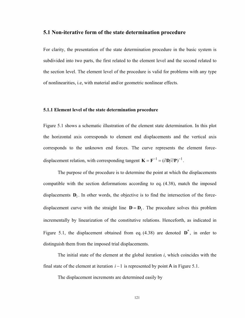
121

5.1 Non-iterative form of the state determination procedure

For clarity, the presentation of the state determination procedure in the basic system is

subdivided into two parts, the first related to the element level and the second related to

the section level. The element level of the procedure is valid for problems with any type

of nonlinearities, i.e, with material and/or geometric nonlinear effects.

5.1.1 Element level of the state determination procedure

Figure 5.1 shows a schematic illustration of the element state determination. In this plot

the horizontal axis corresponds to element end displacements and the vertical axis

corresponds to the unknown end forces. The curve represents the element force-

displacement relation, with corresponding tangent 1 1( )− −= = ∂ ∂K F D P .

The purpose of the procedure is to determine the point at which the displacements

compatible with the section deformations according to eq. (4.38), match the imposed

displacements iD . In other words, the objective is to find the intersection of the force-

displacement curve with the straight line i=D D . The procedure solves this problem

incrementally by linearization of the constitutive relations. Henceforth, as indicated in

Figure 5.1, the displacement obtained from eq. (4.38) are denoted *D , in order to

distinguish them from the imposed trial displacements.

The initial state of the element at the global iteration i, which coincides with the

final state of the element at iteration 1i − is represented by point A in Figure 5.1.

The displacement increments are determined easily by

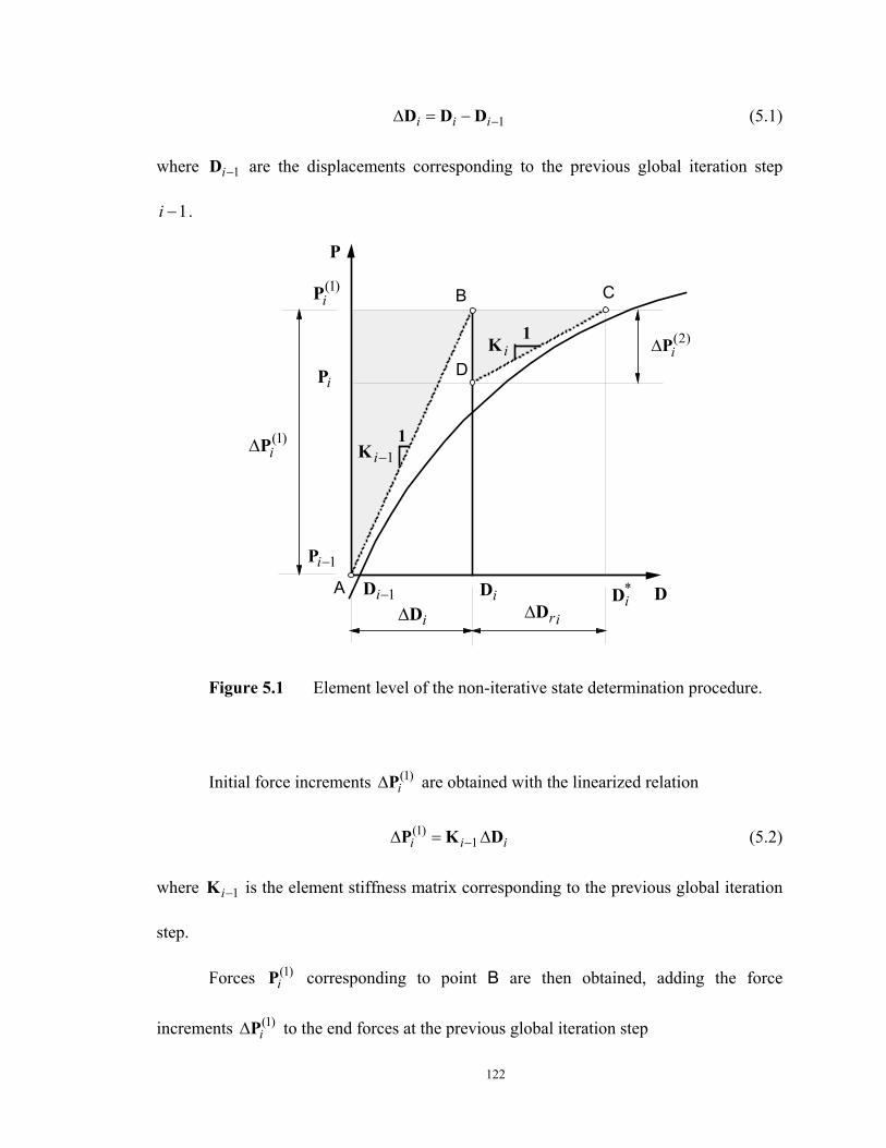
122

1i i i−∆ = −D D D (5.1)

where 1i−D are the displacements corresponding to the previous global iteration step

1i − .

1

1

A

CB

D

K i−1

K i

(1)i∆P

1i−P

iP

(1)iP

P

(2)i∆P

1i−D iD D*iD

ri∆Di∆D

Figure 5.1 Element level of the non-iterative state determination procedure.

Initial force increments (1)i∆P are obtained with the linearized relation

(1)1i ii −∆ = ∆P K D (5.2)

where 1i−K is the element stiffness matrix corresponding to the previous global iteration

step.

Forces (1)iP corresponding to point B are then obtained, adding the force

increments (1)i∆P to the end forces at the previous global iteration step

123

(1) (1)1ii i−= + ∆P P P (5.3)

Associated with the end forces (1)iP , end displacements *

iD corresponding to

point C, and the new element stiffness matrix iK need to be obtained.

For the moment it will be assumed that the displacements *iD and the stiffness

matrix iK can be obtained in terms of the given forces (1)iP as

(1)* ( )i i=D D P (5.4)

(1)( )i i=K K P (5.5)

where the functions ( )D P and ( )K P represent a numerical procedure corresponding to

the sections state determination, which will be presented in the following section. Besides

the argument P, shown explicitly for these functions, other parameters related to the

previous iteration step 1i − (history variables) are also used and need to be stored.

The accuracy of functions ( )D P and ( )K P determines how close point C will be

to the element force-displacement curve. In order to avoid iterations at the section level,

these functions give only a good approximation to the displacements *iD and stiffness

matrix iK . Consequently, as represented in Figure 5.1, point C is slightly off the force-

displacement curve (but still corresponds to the forces (1)iP ). Nonetheless, if iterations

were to be performed at the section level until convergence, point C would lie exactly on

the force-displacement curve, and the stiffness matrix iK would be the exact tangent to

the curve at this point.

After displacements *iD and stiffness matrix iK are computed, residual

124

displacements ri∆D are calculated

*r i ii∆ = −D D D (5.6)

With the updated stiffness matrix iK , an additional force increment (2)i∆P is

determined

(2)i ri i∆ = ∆P K D (5.7)

Finally, element resisting forces iP , corresponding to point D are obtained

(1) (2)i i i= + ∆P P P (5.8)

With this computation, the final state at the end of global iteration i (point D) has

been determined, and will correspond to the initial state for the next global iteration 1i + .

The process is than repeated for the subsequent global iterations.

5.1.2 Section level of the state determination procedure

Consider the problem of finding, for given end forces P, the deformation fields (section

deformations) ( )xd of the materially and geometrically nonlinear supported beam (basic

system) shown in Figure 2.4 for the planar case and Figure 4.2 for the spatial case.

Let d be a composite section deformation vector, defined as

0 1 1

11 1

0

( )( )( )

( ) ( )( )

n nn

nn

ε ξ εκ ξξ κ

ξ εε ξκκ ξ

= ≡ ≡

dd

d(5.9)

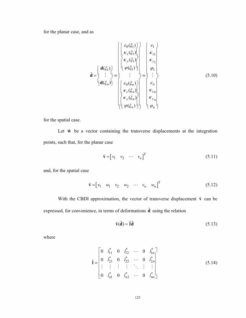
125

for the planar case, and as

0 1 1

1 1

1 1

1 11

0

( )( )( )

( )( )

( ) ( )( )( )

( )

z z

y y

nn n

zz n n

yy n n

n n

ε ξ εκ ξ κκ ξ κ

ϕ ξ ϕξ

εξ ε ξκκ ξκκ ξ

ϕ ξ ϕ

= ≡ ≡

dd

d(5.10)

for the spatial case.

Let w be a vector containing the transverse displacements at the integration

points, such that, for the planar case

[ ]T1 2 nv v v=v (5.11)

and, for the spatial case

[ ]T1 1 2 2 n nv w v w v w=v (5.12)

With the CBDI approximation, the vector of transverse displacement v can be

expressed, for convenience, in terms of deformations d using the relation

( ) =v d ld (5.13)

where

* * *11 12 1* * *21 22 2

* * *1 2

0 0 0

0 0 0

0 0 0

n

n

n n nn

l l l

l l l

l l l

=

l (5.14)

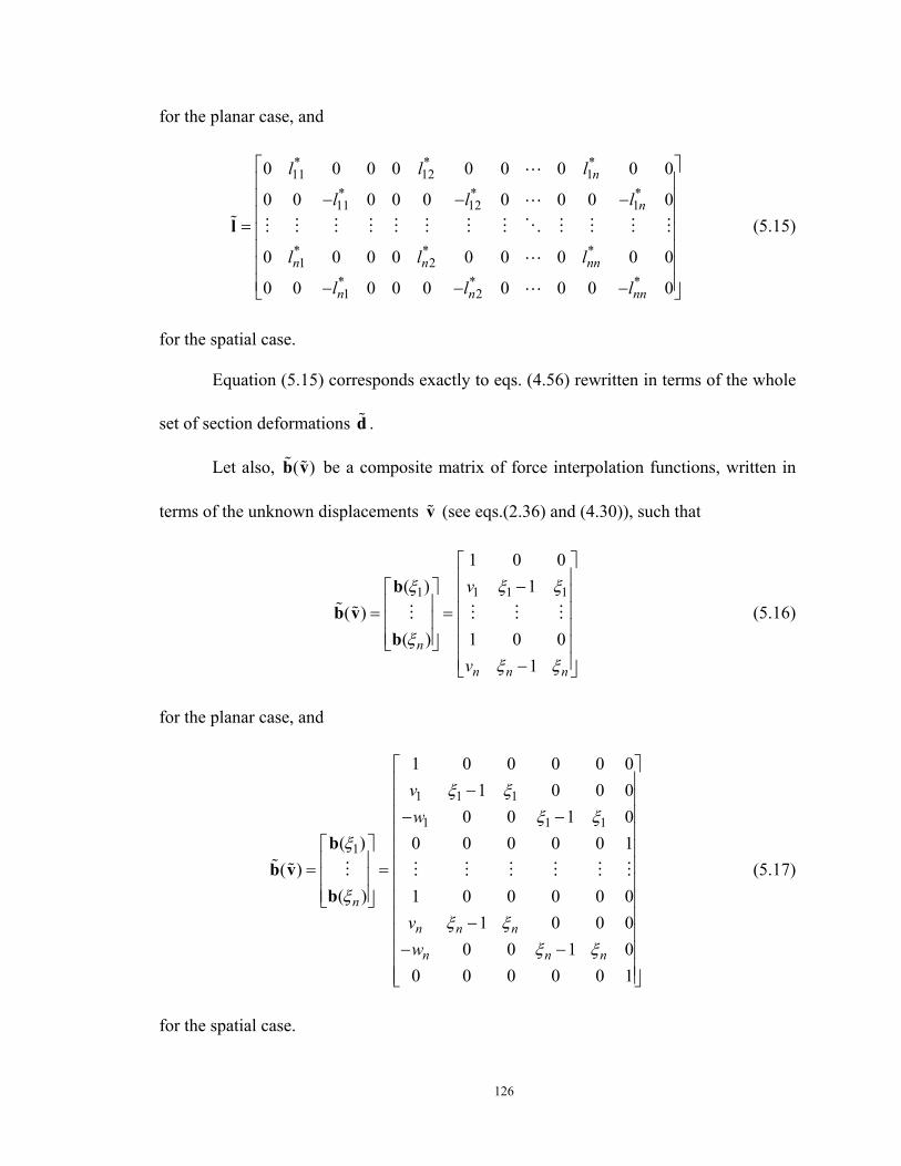
126

for the planar case, and

* * *11 12 1

* * *11 12 1

* * *1 2

* * *1 2

0 0 0 0 0 0 0 0 0

0 0 0 0 0 0 0 0 0

0 0 0 0 0 0 0 0 0

0 0 0 0 0 0 0 0 0

n

n

n n nn

n n nn

l l l

l l l

l l l

l l l

− − − = − − −

l (5.15)

for the spatial case.

Equation (5.15) corresponds exactly to eqs. (4.56) rewritten in terms of the whole

set of section deformations d .

Let also, ( )b v be a composite matrix of force interpolation functions, written in

terms of the unknown displacements v (see eqs.(2.36) and (4.30)), such that

1 1 1 1

1 0 0( ) 1

( )( ) 1 0 0

1n

n n n

v

v

ξ ξ ξ

ξξ ξ

− = = −

bb v

b(5.16)

for the planar case, and

1 1 1

1 1 1

1

1 0 0 0 0 01 0 0 0

0 0 1 0( ) 0 0 0 0 0 1

( )( ) 1 0 0 0 0 0

1 0 0 00 0 1 0

0 0 0 0 0 1

n

n n n

n n n

vw

vw

ξ ξξ ξ

ξ

ξξ ξ

ξ ξ

− − −

= =

− − −

bb v

b(5.17)

for the spatial case.

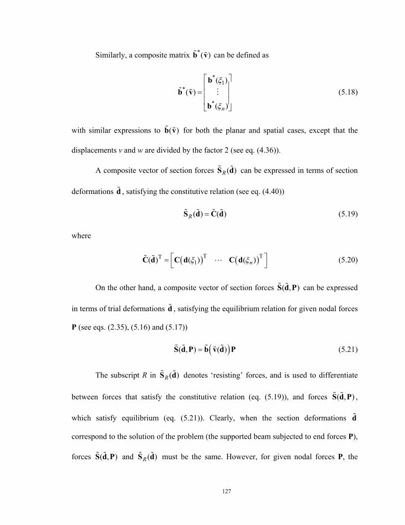
127

Similarly, a composite matrix *( )b v can be defined as

*1

*

*

( )( )

( )n

ξ

ξ

=

bb v

b

(5.18)

with similar expressions to ( )b v for both the planar and spatial cases, except that the

displacements v and w are divided by the factor 2 (see eq. (4.36)).

A composite vector of section forces ( )RS d can be expressed in terms of section

deformations d , satisfying the constitutive relation (see eq. (4.40))

( ) ( )R =S d C d (5.19)

where

( ) ( )T TT1( ) ( ) ( )nξ ξ =

C d C d C d (5.20)

On the other hand, a composite vector of section forces ( , )S d P can be expressed

in terms of trial deformations d , satisfying the equilibrium relation for given nodal forces

P (see eqs. (2.35), (5.16) and (5.17))

( )( , ) ( )=S d P b v d P (5.21)

The subscript R in ( )RS d denotes ‘resisting’ forces, and is used to differentiate

between forces that satisfy the constitutive relation (eq. (5.19)), and forces ( , )S d P ,

which satisfy equilibrium (eq. (5.21)). Clearly, when the section deformations d

correspond to the solution of the problem (the supported beam subjected to end forces P),

forces ( , )S d P and ( )RS d must be the same. However, for given nodal forces P, the

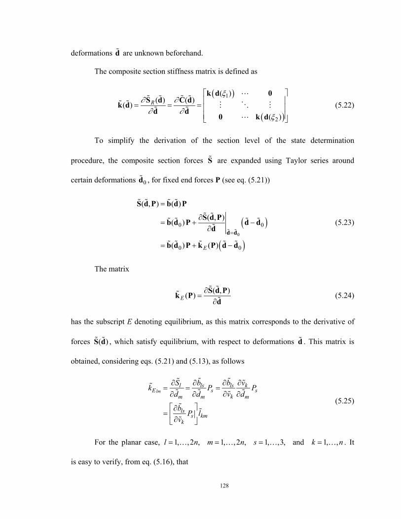
128

deformations d are unknown beforehand.

The composite section stiffness matrix is defined as

( )

( )

1

2

( )( ) ( )( )

( )

Rξ

∂ ∂∂ ∂

ξ

= = =

k d 0S d C dk d

d d0 k d

(5.22)

To simplify the derivation of the section level of the state determination

procedure, the composite section forces S are expanded using Taylor series around

certain deformations 0d , for fixed end forces P (see eq. (5.21))

( )

( )0

0 0

0 0

( , ) ( )

( , )( )

( ) ( )E

=

=

∂= + −

∂

= + −

d d

S d P b d P

S d Pb d P d dd

b d P k P d d

(5.23)

The matrix

( , )( )E∂

=∂

S d Pk Pd

(5.24)

has the subscript E denoting equilibrium, as this matrix corresponds to the derivative of

forces ( )S d , which satisfy equilibrium, with respect to deformations d . This matrix is

obtained, considering eqs. (5.21) and (5.13), as follows

lml ls ls k

E s skm m m

lss km

k

S b b vk P Pvd d d

b P lv

∂ ∂ ∂ ∂= = =

∂∂ ∂ ∂

∂= ∂

(5.25)

For the planar case, 1, ,2 , 1, ,2 , 1, ,3, and 1, ,l n m n s k n= = = =… … … … . It

is easy to verify, from eq. (5.16), that

129

1

0 0 01 0 00 0 00 1 0

0 0 00 0 1

lss

k

kl

b PPv

∂∂

→

↓

=

(5.26)

Thus, for the planar case, Ek can be obtained by multiplying the matrix given in

eq. (5.26) by matrix l given in eq. (5.14). The result can be expressed as

* * *11 12 1* * *21 22 2

1

* * *1 2 22

( ) ( ) ( )

( ) ( ) ( )( )

( ) ( ) ( )

n

nE E

n n

l l l

l l l P

l l l

≡ =

s s s

s s sk k P

s s s

(5.27)

with

**

0 0( )

0ijij

ll

=

s (5.28)

For the spatial case, the derivation is similar to the planar case, with

1, ,4 , 1, ,4 , 1, ,6, and 1, ,2l n m n s k n= = = =… … … … , and can be expressed in the

same way as in eq. (5.27), but with

**

*

0 0 0 0

0 0 0( )

0 0 0

0 0 0 0

ijij

ij

ll

l

= −

s (5.29)

Although matrix Ek depends only on the component 1P (the axial force) of the

130

force vector P, the notation ( )Ek P is preferred to avoid excessive use of indices in the

derivations that follows, when indices related to iteration steps will be introduced.

As matrix ( )Ek P does not depend on the deformations d , the forces ( , )S d P are,

for fixed forces P, a linear function of d . Thus, the expansion (5.23) is exact with the

first two terms only, i.e., the other higher order terms are null.

Another important consideration is that, despite of the fact that matrix ( )k d is a

super-diagonal matrix, matrix ( )Ek P is not. As a consequence, the problem of

determining the section deformations d for given end forces P is coupled through the

sections. Thus, the section determination procedure cannot be performed for each section

individually, but has to be done considering all the sections at the same time. To this end,

a simultaneous section state determination procedure is proposed.

Figure 5.2 shows a schematic representation of the section level of the procedure.

In this plot, the horizontal axis corresponds to the unknown composite section

deformations and the vertical axis corresponds to composite section forces. The curved

line represents the force-deformation relation ( ) ( )R =S d C d , with corresponding tangent

( ) ( )R= ∂ ∂k d S d d . The straight line with slope (1)( )E ik P represents the applied section

forces ( , )S d P , in equilibrium with element end forces (1)iP .

The purpose of the procedure is to determine, for forces (1)iP , the point at which

the resisting forces ( )RS d equilibrate the applied forces (1)( , )iS d P . This corresponds to

finding the intersection of the curve ( )RS d with the straight line (1)( , )iS d P .

The proposed algorithm solves this problem incrementally, by linearizing the

131

section constitutive relations ( ) ( )R =S d C d using the tangent composite section stiffness

( )k d , as shown in Figure 5.2.

The three points A, B, and C in Figure 5.2 also correspond to the respective points

in Figure 5.1. The initial state of the sections at the global iteration 1i − is represented by

point A, and the first phase consists in determining point B, i.e., determining

deformations (1)id and corresponding forces (1)

iS . Then, point C is determined. This is

accomplished as follows.

11

1

B

C

A ~di−1~( )di

1 ~di

∆~( )di1 ∆~( )di

2

~k i−1

~ki

(1)( )E ik P

~d

(1)i∆S

(2)i∆S (0)

iS

(1)iSiS

1i−S

(1)i∆S

S

RiS

Figure 5.2 Section level of the state determination procedure

First, section forces (0)iS in equilibrium with end forces (1)

iP for 1i−=d d are

computed according to eq. (5.21)

132

( )(0) (1)1( )ii i−=S b v d P (5.30)

Then, the corresponding section force increments from the previous state are

determined

( )(1) (0) (1)1 1 1( )i i ii i i− − −∆ = − = −S S S b v d P S (5.31)

With the composite section stiffness matrix 1i−k from the previous iteration step,

and force increments (1)i∆S , deformation increments (1)

i∆d are obtained according to

Figure 5.2.

1(1) (1) (1)1( )E ii i i

−− ∆ = − − ∆ d k P k S (5.32)

With this, the section deformations can be updated, giving (1)id

(1) (1)1ii i−= + ∆d d d (5.33)

Forces (1)iS corresponding to point B can then be calculated according to

eq. (5.21) or (5.23)

(1) (1) (1)

(1) (1) (1)1

(0) (1) (1)

( )

( ) ( )

( )

i i i

i Ei i i

Ei i i

−

=

= + ∆

= + ∆

S b d P

b d P k P d

S k P d

(5.34)

Corresponding to deformations (1)id , resisting forces RiS and the new composite

section stiffness matrix ik can be computed using the section constitutive relation (eq.

(5.19) and corresponding linearization (5.22))

(1)( )R ii =S C d (5.35)

133

(1)( )i i=k k d (5.36)

The unbalanced section forces are given by

(2) (1)Ri i i∆ = −S S S (5.37)

Then, the deformations corresponding to point C are calculated with the new

stiffness matrix ik

1(2) (1) (2)( )E ii i i−

∆ = − − ∆ d k P k S (5.38)

(1) (2)i i i= + ∆d d d (5.39)

Once the section deformations id have been determined, forces iS corresponding

to point C can then be calculated according to eq. (5.21) or (5.23)

(1)( )i i i=S b d P (5.40)

Element end displacements *iD corresponding to point C can be computed by

numerical integration of eq. (4.38)

* * T

1( ) ( )

n

i j i j jj

L Wξ ξ=

= ∑D b d (5.41)

where jW are the integration weights for the interval [0,1]. The section deformations

( )i jξd are extracted from the composite deformation vector id . The displacements jv

and jw necessary for the computation of matrix *( )jξb are obtained in terms of

deformations id using the CBDI procedure according to eq. (5.13).

The element flexibility matrix is determined by numerical integration of

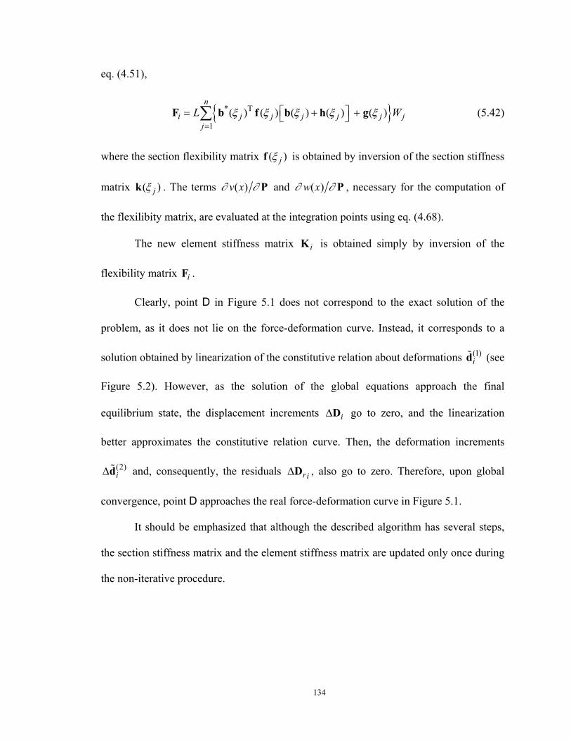
134

eq. (4.51),

* T

1( ) ( ) ( ) ( ) ( )

n

i j j j j j jj

L Wξ ξ ξ ξ ξ=

= + + ∑F b f b h g (5.42)

where the section flexibility matrix ( )jξf is obtained by inversion of the section stiffness

matrix ( )jξk . The terms ( )v x∂ ∂ P and ( )w x∂ ∂ P , necessary for the computation of

the flexilibity matrix, are evaluated at the integration points using eq. (4.68).

The new element stiffness matrix iK is obtained simply by inversion of the

flexibility matrix iF .

Clearly, point D in Figure 5.1 does not correspond to the exact solution of the

problem, as it does not lie on the force-deformation curve. Instead, it corresponds to a

solution obtained by linearization of the constitutive relation about deformations (1)id (see

Figure 5.2). However, as the solution of the global equations approach the final

equilibrium state, the displacement increments i∆D go to zero, and the linearization

better approximates the constitutive relation curve. Then, the deformation increments

(2)i∆d and, consequently, the residuals ri∆D , also go to zero. Therefore, upon global

convergence, point D approaches the real force-deformation curve in Figure 5.1.

It should be emphasized that although the described algorithm has several steps,

the section stiffness matrix and the element stiffness matrix are updated only once during

the non-iterative procedure.

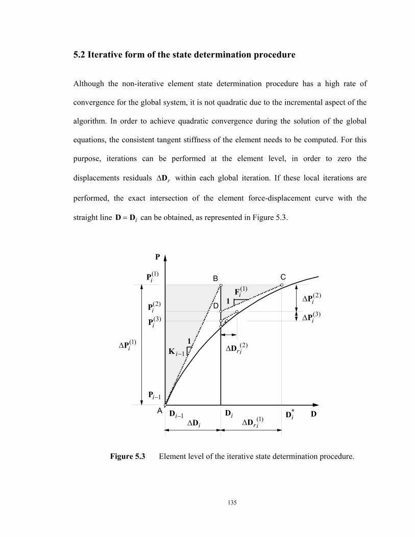
135

5.2 Iterative form of the state determination procedure

Although the non-iterative element state determination procedure has a high rate of

convergence for the global system, it is not quadratic due to the incremental aspect of the

algorithm. In order to achieve quadratic convergence during the solution of the global

equations, the consistent tangent stiffness of the element needs to be computed. For this

purpose, iterations can be performed at the element level, in order to zero the

displacements residuals r∆D within each global iteration. If these local iterations are

performed, the exact intersection of the element force-displacement curve with the

straight line i=D D can be obtained, as represented in Figure 5.3.

1

1

A

CB

D

Fi( )1

K i−1

(1)i∆P

1i−P

P

1i−D iD *iD

i∆D (1)ri∆D

(2)ri∆D

(1)iP

(2)iP

(2)i∆P

(3)i∆P(3)

iP

D

Figure 5.3 Element level of the iterative state determination procedure.

136

The iterative procedure is easily accomplished, and consists in a generalization of

the non-iterative procedure described above. First, point D is determined following the

same steps of the non-iterative procedure. Then, the end forces are updated from (1)iP to

(2)iP . After this update, the section level of the state determination procedure is executed

again, with the new forces (2)iP . The end forces are then update to (3)

iP , and the

procedure is repeated until some convergence criteria is satisfied (e.g., tolr∆ ≤D , where

tol is a given tolerance). Figure 5.4 shows the corresponding pseudo code of the state

determination procedure performed in the basic system.

From the pseudo code, it can be confirmed that the non-iterative version of the

state determination procedure is a particularization of the iterative algorithm, when the

specified maximum number of local iterations is set equal to 1.

In the iterative procedure, a consistent element tangent stiffness is obtained

(within specified tolerance), and quadratic convergence is obtained. As the non-iterative

procedure solves the problem incrementally, the element tangent stiffness matrix is

approximate during the initial global iterative solution. However, as the global iterative

strategy proceeds, the displacement increments decrease, and the computed element

stiffness better approximates the exact tangent stiffness. However, it is observed that

convergence is almost quadratic and is practically as fast as the one obtained with the

iterative solution.

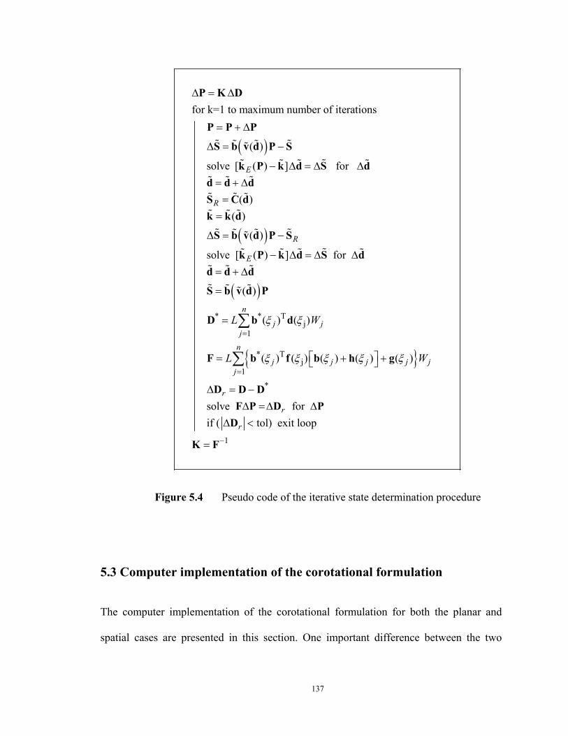
137

( )

( )

( )

for k=1 to maximum number of iterations

( )

solve [ ( ) ] for

( )( )

( )

solve [ ( ) ] for

( )

E

R

R

E

∆ = ∆

= + ∆

∆ = −

− ∆ = ∆ ∆= + ∆=

=

∆ = −

− ∆ = ∆ ∆= + ∆

=

P K D

P P P

S b v d P S

k P k d S dd d dS C dk k d

S b v d P S

k P k d S dd d d

S b v d P

* * Tj

1

* Tj

1

*

1

( ) ( )

( ) ( ) ( ) ( ) ( )

solve for if ( tol) exit loop

n

j jj

n

j j j j jj

r

r

r

L W

L W

ξ ξ

ξ ξ ξ ξ ξ

=

=

−

=

= + +

∆ = −∆ =∆ ∆

∆ <

=

∑

∑

D b d

F b f b h g

D D DF P D P

D

K F

Figure 5.4 Pseudo code of the iterative state determination procedure

5.3 Computer implementation of the corotational formulation

The computer implementation of the corotational formulation for both the planar and

spatial cases are presented in this section. One important difference between the two

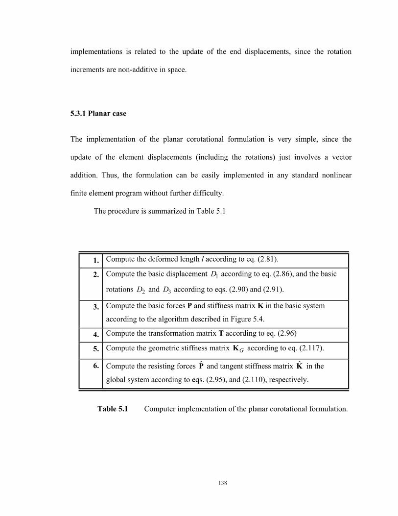
138

implementations is related to the update of the end displacements, since the rotation

increments are non-additive in space.

5.3.1 Planar case

The implementation of the planar corotational formulation is very simple, since the

update of the element displacements (including the rotations) just involves a vector

addition. Thus, the formulation can be easily implemented in any standard nonlinear

finite element program without further difficulty.

The procedure is summarized in Table 5.1

1. Compute the deformed length l according to eq. (2.81).

2. Compute the basic displacement 1D according to eq. (2.86), and the basic

rotations 2D and 3D according to eqs. (2.90) and (2.91).

3. Compute the basic forces P and stiffness matrix K in the basic system

according to the algorithm described in Figure 5.4.

4. Compute the transformation matrix T according to eq. (2.96)

5. Compute the geometric stiffness matrix GK according to eq. (2.117).

6. Compute the resisting forces P and tangent stiffness matrix K in the

global system according to eqs. (2.95), and (2.110), respectively.

Table 5.1 Computer implementation of the planar corotational formulation.

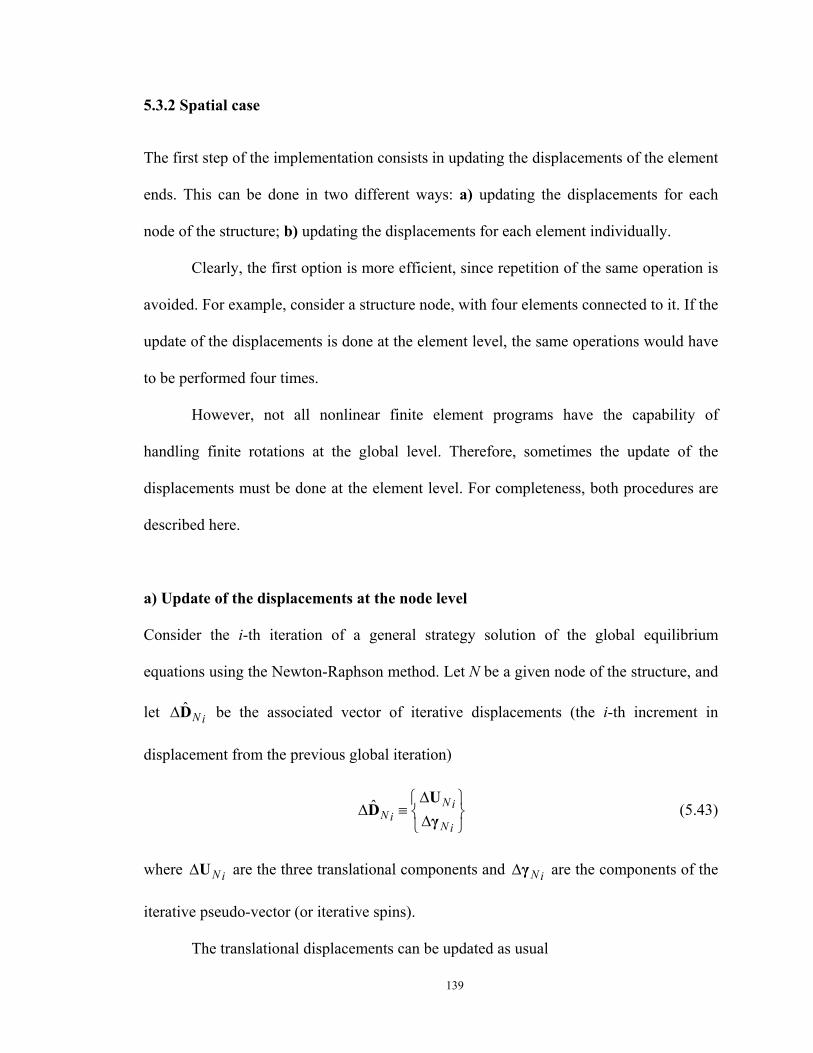
139

5.3.2 Spatial case

The first step of the implementation consists in updating the displacements of the element

ends. This can be done in two different ways: a) updating the displacements for each

node of the structure; b) updating the displacements for each element individually.

Clearly, the first option is more efficient, since repetition of the same operation is

avoided. For example, consider a structure node, with four elements connected to it. If the

update of the displacements is done at the element level, the same operations would have

to be performed four times.

However, not all nonlinear finite element programs have the capability of

handling finite rotations at the global level. Therefore, sometimes the update of the

displacements must be done at the element level. For completeness, both procedures are

described here.

a) Update of the displacements at the node level

Consider the i-th iteration of a general strategy solution of the global equilibrium

equations using the Newton-Raphson method. Let N be a given node of the structure, and

let ˆN i∆D be the associated vector of iterative displacements (the i-th increment in

displacement from the previous global iteration)

ˆ N iN i

N i

∆ ∆ ≡ ∆

UD

γ(5.43)

where N i∆U are the three translational components and N i∆γ are the components of the

iterative pseudo-vector (or iterative spins).

The translational displacements can be updated as usual

140

1N N Ni i i−= + ∆U U U (5.44)

However, as the rotational vectors are not additive, to update the node rotational

components, the compound rotation formula needs to be used

1( ) ( ) ( )N N Ni i i−= ∆R γ R γ R γ (5.45)

Usually, it is not necessary to extract the pseudo vector N iγ from the rotation

matrix ( )N iR γ , since the rotation matrix itself can be passed to the elements. Besides, as

discussed before, the extraction of the pseudo-vector is only unique for rotations with

magnitude less than 180 degrees. As discussed in Section 3.5, the extraction can be

performed using the normalized quaternions.

However, it is more efficient to use the quaternion product, given by eq. (3.54),

such that

1N N Ni i i−= ∆q q q (5.46)

where 1N i−q and N i∆q are the normalized quaternions associated with rotational vectors

1N i−γ and N i∆γ , respectively, via eq. (3.44). After the unit quaternion N iq , has been

obtained, the associated rotation matrix ( )N iR q can be computed according to eq. (3.50).

With this computation, the normalized quaternions and/or the associated rotation

matrices corresponding to nodes N I= and N J= can be passed to the elements. The

element end triads than can be updated as

0

0

( )

( )I I Ii i

J J Ji i

=

=

N R N

N R N

q

q(5.47)

with 0IN and 0JN being the initial triads given in eq. (4.77). However, here again it is

141

more efficient to use the quaternion product, such that

0

0

I I Ii i

J J Ji i

=

=

n n

n n

q

q(5.48)

where I in and J in are the unit quaternions associated to the triads I iN and J iN ,

respectively.

b) Update of the displacements at the element level

Given the iterative global displacement vector ˆi∆D of the element, its translational

components can be updated as usual, as in eq. (5.44), with N I= and N J=

1

1

I I Ii i i

J J Ji i i

−

−

= + ∆

= + ∆

U U UU U U

(5.49)

The element end triads can then be updated with the compound rotation formula

1

1

( )( )

I I Ii i i

J J Ji i i

−

−

= ∆

= ∆

N R γ NN R γ N

(5.50)

However, here again it is more efficient to use the unit quaternions, such that

1

1

I Ii iI i

J Ji iJ i

−

−

= ∆

= ∆

n n

n n

q

q(5.51)

where I i∆q and J i∆q are the unit quaternions associated with the rotational vectors

I i∆γ and J i∆γ , respectively. The triads I iN and J iN can then be obtained from the unit

quaternions I in and J in , via eq. (3.50)

A summarized description of the computational procedure involved in the

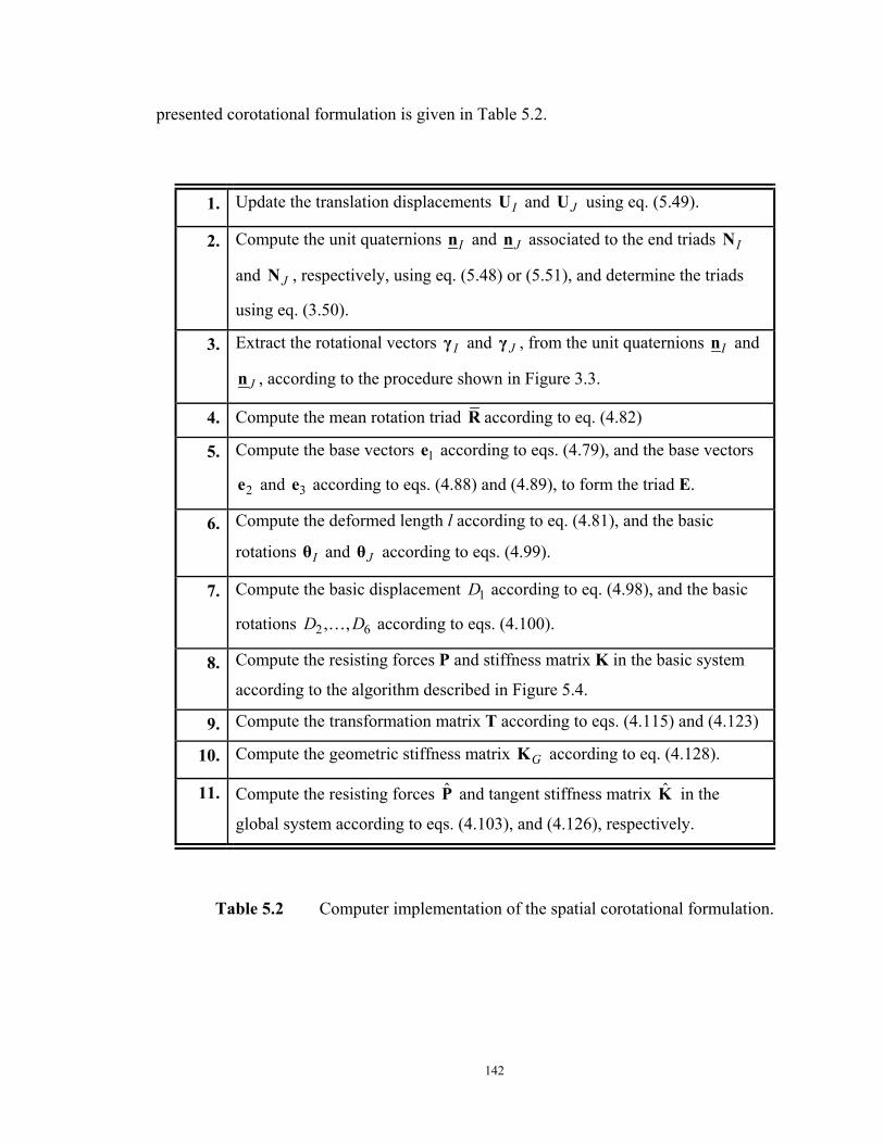
142

presented corotational formulation is given in Table 5.2.

1. Update the translation displacements IU and JU using eq. (5.49).

2. Compute the unit quaternions In and Jn associated to the end triads IN

and JN , respectively, using eq. (5.48) or (5.51), and determine the triads

using eq. (3.50).

3. Extract the rotational vectors Iγ and Jγ , from the unit quaternions In and

Jn , according to the procedure shown in Figure 3.3.

4. Compute the mean rotation triad R according to eq. (4.82)

5. Compute the base vectors 1e according to eqs. (4.79), and the base vectors

2e and 3e according to eqs. (4.88) and (4.89), to form the triad E.

6. Compute the deformed length l according to eq. (4.81), and the basic

rotations Iθ and Jθ according to eqs. (4.99).

7. Compute the basic displacement 1D according to eq. (4.98), and the basic

rotations 2 6, ,D D… according to eqs. (4.100).

8. Compute the resisting forces P and stiffness matrix K in the basic system

according to the algorithm described in Figure 5.4.

9. Compute the transformation matrix T according to eqs. (4.115) and (4.123)

10. Compute the geometric stiffness matrix GK according to eq. (4.128).

11. Compute the resisting forces P and tangent stiffness matrix K in the

global system according to eqs. (4.103), and (4.126), respectively.

Table 5.2 Computer implementation of the spatial corotational formulation.

143

5.4 Update of history variables

Following the proposed state determination procedures, in additional to material history

variables, the following variables need to be stored for each element: basic end forces P,

basic stiffness matrix K, section deformations d , section forces S , and section stiffness

k . An example of material history variable that may need to be stored is the plastic strain

of each integration point over the section, when a ‘fiber-section’ discretization is used

with elasto-plastic material.

Regarding the update of the rotational displacement components in space, it is

also necessary to store the unit quaternions associated to the rotational vectors. If the

procedure (a) described in Section 5.3.2 is adopted, the unit quaternion N iq of each node

of the structure need to be stored. Alternatively, if procedure (b) is adopted, then, the two

unit quaternions I in and J in associated to the end triads, need to be stored for each

element.

However, although the material history variables should only be updated upon

global convergence, the other variables P, K, d , D , k , and the normalized quaternions

are updated after each iteration.

144

Chapter 6Numerical Examples

In order to validate the proposed element and to test its accuracy, some examples were

solved and the solutions are compared with those obtained by other authors. For some

planar problems, an analytical linear elastic solution, when available, is also shown for

comparison.

Is should be emphasized that, as most papers only provide the results in graphical

form, only a reasonable accurate comparison can be done, due to the inaccuracy in

obtaining numerical values from the presented plots.

The state determination procedure without local iterations was used to obtain all

the results corresponding to the proposed formulation. As discussed previously, if local

iterations are performed at the element level, although the total number of iterations may

be smaller, the overall performance is worse since a large amount of processing time is

spent in the element state determination procedure.

Unless otherwise indicated in the following examples, for the solution of the

nonlinear global equations, the global iterative strategy used is the ‘minimum residual

displacement method’, proposed by Chan (1988), with an updated stiffness matrix at each

iteration (classical Newton-Raphson). The load incrementation was performed using the

‘incrementation of the arc-length’ procedure as described by Clarke and Hancock (1990).

The marks shown in the plots for the present formulation correspond to each load step.

The convergence criterion is based on the relative energy norm.

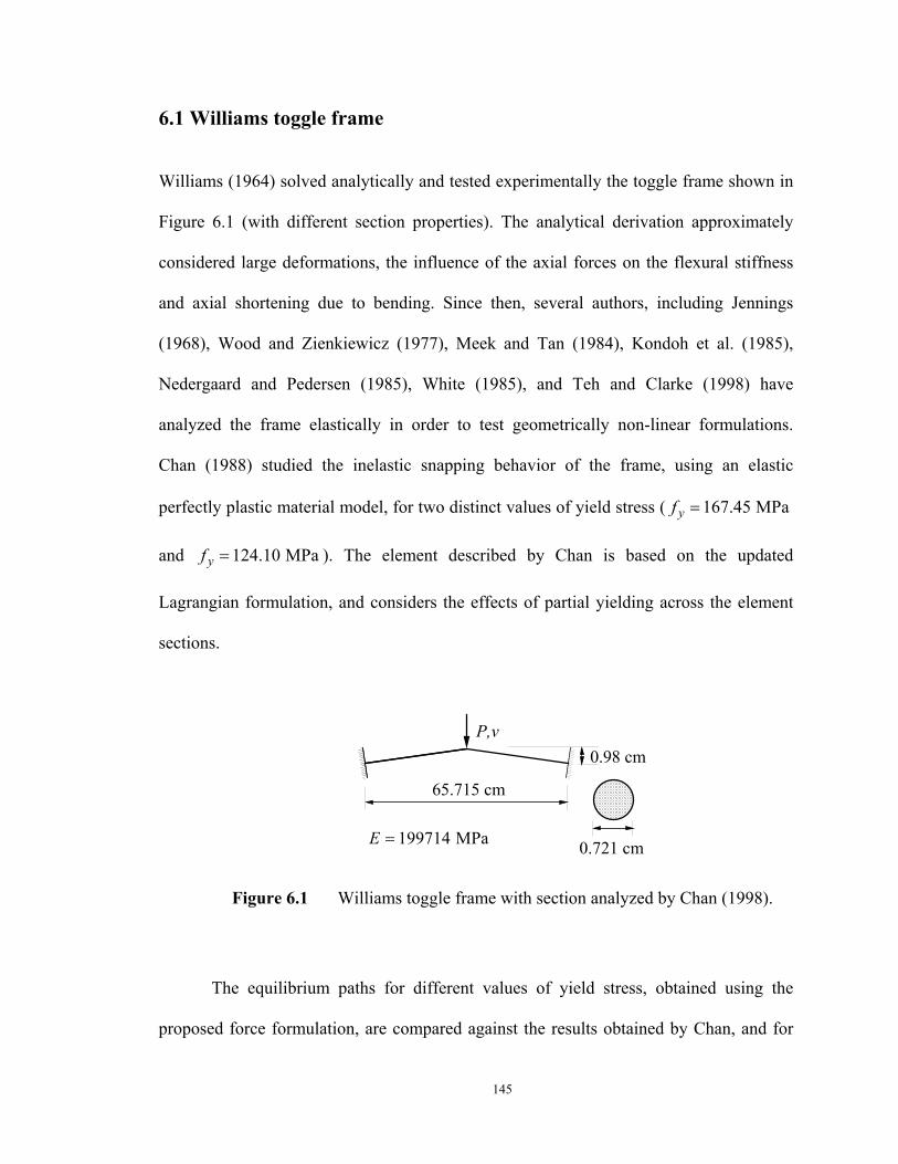
145

6.1 Williams toggle frame

Williams (1964) solved analytically and tested experimentally the toggle frame shown in

Figure 6.1 (with different section properties). The analytical derivation approximately

considered large deformations, the influence of the axial forces on the flexural stiffness

and axial shortening due to bending. Since then, several authors, including Jennings

(1968), Wood and Zienkiewicz (1977), Meek and Tan (1984), Kondoh et al. (1985),

Nedergaard and Pedersen (1985), White (1985), and Teh and Clarke (1998) have

analyzed the frame elastically in order to test geometrically non-linear formulations.

Chan (1988) studied the inelastic snapping behavior of the frame, using an elastic

perfectly plastic material model, for two distinct values of yield stress ( 167.45 MPayf =

and 124.10 MPayf = ). The element described by Chan is based on the updated

Lagrangian formulation, and considers the effects of partial yielding across the element

sections.

0.98 cmP,v

E = 199714 MPa 0.721 cm

65.715 cm

Figure 6.1 Williams toggle frame with section analyzed by Chan (1998).

The equilibrium paths for different values of yield stress, obtained using the

proposed force formulation, are compared against the results obtained by Chan, and for

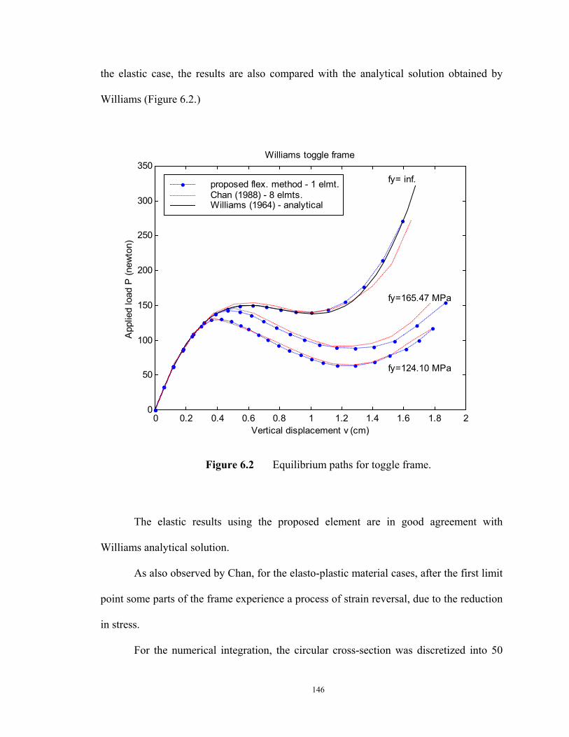
146

the elastic case, the results are also compared with the analytical solution obtained by

Williams (Figure 6.2.)

0 0.2 0.4 0.6 0.8 1 1.2 1.4 1.6 1.8 20

50

100

150

200

250

300

350

Vertical displacement v (cm)

App

lied

load

P (n

ewto

n)

Williams toggle frame

fy=124.10 MPa

fy=165.47 MPa

fy= inf.proposed flex. method - 1 elmt.Chan (1988) - 8 elmts.Williams (1964) - analytical

Figure 6.2 Equilibrium paths for toggle frame.

The elastic results using the proposed element are in good agreement with

Williams analytical solution.

As also observed by Chan, for the elasto-plastic material cases, after the first limit

point some parts of the frame experience a process of strain reversal, due to the reduction

in stress.

For the numerical integration, the circular cross-section was discretized into 50

147

layers, and the midpoint rule was employed.

An interesting fact was observed in this example regarding the necessary number

of iterations per load step. Due to the symmetry of the frame, and the fact that only one

element is being used to model the structure, this problem has only one degree of

freedom (vertical displacement at the apex). For structures with one degree of freedom

only, the minimum residual displacement method particularizes to the displacement

control method (see Clarke and Hancock (1990)), which automatically converges upon

the second iteration in this case.

However, for the second value of the yield stress 124.10 MPayf = convergence

to the reported solution was difficult to achieve, as the structure tended to converge to

another path, around the displacement v = 1 cm, which was not reported by Chan.

6.2 Simply supported beam with uniform load

The beam shown in Figure 6.3 was analyzed numerically by Backlund (1976)

considering different combinations of the two sources of nonlinearity (geometric and

material). The same problem type, but with different parameters, was analyzed by

Coulter and Miller (1988), considering both sources of nonlinearities, geometric and

material. An analytical solution is presented in Timoshenko and Woinowsky-Krieger

(1959).

Although the consideration of distributed loads was not presented in the

derivation of the element formulation in Chapter 2, this example is used to illustrate the

applicability of the proposed method to structures subject to uniform load. The inclusion

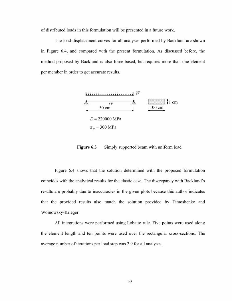
148

of distributed loads in this formulation will be presented in a future work.

The load-displacement curves for all analyses performed by Backlund are shown

in Figure 6.4, and compared with the present formulation. As discussed before, the

method proposed by Backlund is also force-based, but requires more than one element

per member in order to get accurate results.

50 cm

W

v

E

y

=

=

220000

300

MPa

MPaσ

1 cm100 cm

Figure 6.3 Simply supported beam with uniform load.

Figure 6.4 shows that the solution determined with the proposed formulation

coincides with the analytical results for the elastic case. The discrepancy with Backlund’s

results are probably due to inaccuracies in the given plots because this author indicates

that the provided results also match the solution provided by Timoshenko and

Woinowsky-Krieger.

All integrations were performed using Lobatto rule. Five points were used along

the element length and ten points were used over the rectangular cross-sections. The

average number of iterations per load step was 2.9 for all analyses.

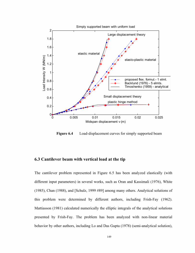
149

0 0.005 0.01 0.015 0.02 0.0250

0.2

0.4

0.6

0.8

1

1.2

1.4

1.6

1.8

2Simply supported beam with uniform load

Midspan displacement v (m)

Load

Inte

nsity

W (M

N/m

)

Large displacement theory

elastic material

elasto-plastic material

Small displacement theory

plastic hinge method

proposed flex. formul.- 1 elmt.Backlund (1976) - 5 elmts.Timoshenko (1959) - analytical

Figure 6.4 Load-displacement curves for simply supported beam

6.3 Cantilever beam with vertical load at the tip

The cantilever problem represented in Figure 6.5 has been analyzed elastically (with

different input parameters) in several works, such as Oran and Kassimali (1976), White

(1985), Chan (1988), and [Schulz, 1999 #89] among many others. Analytical solutions of

this problem were determined by different authors, including Frish-Fay (1962).

Mattiasson (1981) calculated numerically the elliptic integrals of the analytical solutions

presented by Frish-Fay. The problem has been analyzed with non-linear material

behavior by other authors, including Lo and Das Gupta (1978) (semi-analytical solution),

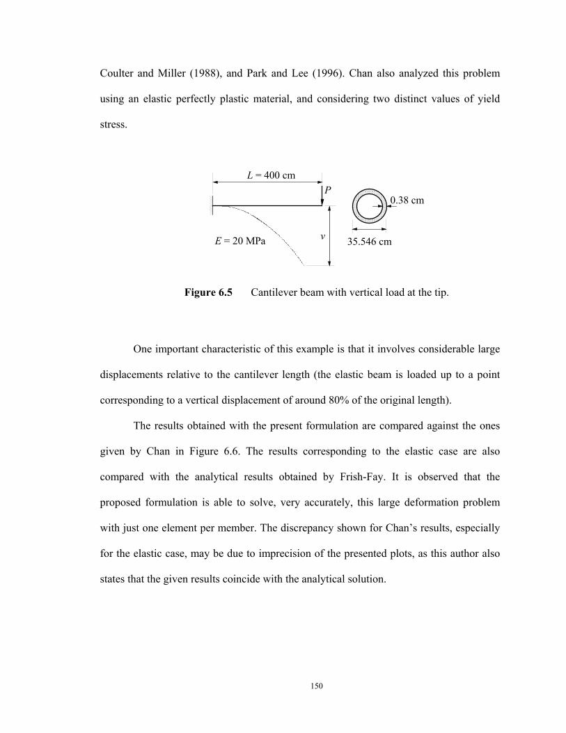
150

Coulter and Miller (1988), and Park and Lee (1996). Chan also analyzed this problem

using an elastic perfectly plastic material, and considering two distinct values of yield

stress.

L = 400 cm

v

P

35.546 cmE = 20 MPa

0.38 cm

Figure 6.5 Cantilever beam with vertical load at the tip.

One important characteristic of this example is that it involves considerable large

displacements relative to the cantilever length (the elastic beam is loaded up to a point

corresponding to a vertical displacement of around 80% of the original length).

The results obtained with the present formulation are compared against the ones

given by Chan in Figure 6.6. The results corresponding to the elastic case are also

compared with the analytical results obtained by Frish-Fay. It is observed that the

proposed formulation is able to solve, very accurately, this large deformation problem

with just one element per member. The discrepancy shown for Chan’s results, especially

for the elastic case, may be due to imprecision of the presented plots, as this author also

states that the given results coincide with the analytical solution.

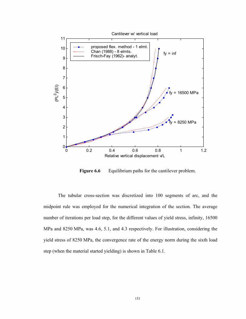
151

0 0.2 0.4 0.6 0.8 1 1.20

1

2

3

4

5

6

7

8

9

10

11Cantilever w/ vertical load

Relative vertical displacement v/L

(PL2 )/(

EI)

fy = inf

fy = 16500 MPa

fy = 8250 MPa

proposed flex. method - 1 elmt.Chan (1988) - 8 elmts.Frisch-Fay (1962)- analyt.

Figure 6.6 Equilibrium paths for the cantilever problem.

The tubular cross-section was discretized into 100 segments of arc, and the

midpoint rule was employed for the numerical integration of the section. The average

number of iterations per load step, for the different values of yield stress, infinity, 16500

MPa and 8250 MPa, was 4.6, 5.1, and 4.3 respectively. For illustration, considering the

yield stress of 8250 MPa, the convergence rate of the energy norm during the sixth load

step (when the material started yielding) is shown in Table 6.1.

152

Iteration Relative energy norm

1 1.0

2 4.919771934662989e-002

3 2.641579924599226e-004

4 5.790622677740988e-009

Table 6.1 Convergence rate for cantilever problem at load step 6.

6.4 Cantilever beam under a moment at the tip

The classical problem of a cantilever beam subject to a moment at the free end is

illustrated in Figure 6.7. This problem has been analyzed by a number of researchers

including Bathe and Bolourchi (1979), Simo and Vu-Quoc (1986), Crisfield (1990),

Gummadi and Palazotto (1998), Waszczyszyn and Janus-Michalska (1998) and Schulz

and Filippou (2000) in order to test the accuracy of the proposed elements under extreme

inextensional bending.

L

v

u

2 EIMLπ

=

Figure 6.7 Cantilever subjected to end moment.

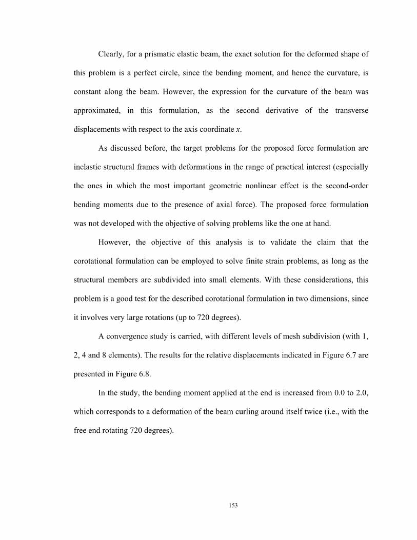
153

Clearly, for a prismatic elastic beam, the exact solution for the deformed shape of

this problem is a perfect circle, since the bending moment, and hence the curvature, is

constant along the beam. However, the expression for the curvature of the beam was

approximated, in this formulation, as the second derivative of the transverse

displacements with respect to the axis coordinate x.

As discussed before, the target problems for the proposed force formulation are

inelastic structural frames with deformations in the range of practical interest (especially

the ones in which the most important geometric nonlinear effect is the second-order

bending moments due to the presence of axial force). The proposed force formulation

was not developed with the objective of solving problems like the one at hand.

However, the objective of this analysis is to validate the claim that the

corotational formulation can be employed to solve finite strain problems, as long as the

structural members are subdivided into small elements. With these considerations, this

problem is a good test for the described corotational formulation in two dimensions, since

it involves very large rotations (up to 720 degrees).

A convergence study is carried, with different levels of mesh subdivision (with 1,

2, 4 and 8 elements). The results for the relative displacements indicated in Figure 6.7 are

presented in Figure 6.8.

In the study, the bending moment applied at the end is increased from 0.0 to 2.0,

which corresponds to a deformation of the beam curling around itself twice (i.e., with the

free end rotating 720 degrees).

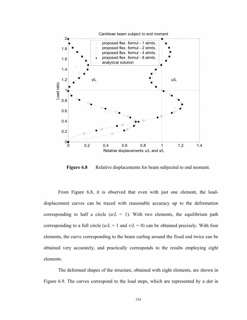
154

0 0.2 0.4 0.6 0.8 1 1.2 1.40

0.2

0.4

0.6

0.8

1

1.2

1.4

1.6

1.8

2Cantilever beam subject to end moment

Relative displacements u/L and v/L

Load

ratio

v/L u/L

proposed flex. formul - 1 elmts.proposed flex. formul - 2 elmts.proposed flex. formul - 4 elmts.proposed flex. formul - 8 elmts.analytical solution

Figure 6.8 Relative displacements for beam subjected to end moment.

From Figure 6.8, it is observed that even with just one element, the load-

displacement curves can be traced with reasonable accuracy up to the deformation

corresponding to half a circle (u/L = 1). With two elements, the equilibrium path

corresponding to a full circle (u/L = 1 and v/L = 0) can be obtained precisely. With four

elements, the curve corresponding to the beam curling around the fixed end twice can be

obtained very accurately, and practically corresponds to the results employing eight

elements.

The deformed shapes of the structure, obtained with eight elements, are shown in

Figure 6.9. The curves correspond to the load steps, which are represented by a dot in

155

Figure 6.8. The average number of iterations per load step was 5.10.

-0.2 -0.1 0 0.1 0.2 0.3 0.4 0.5 0.6 0.70

0.1

0.2

0.3

0.4

0.5

0.6

0.7

Cantilever beam subject to end moment

x

y

Figure 6.9 Deformed shapes for the cantilever beam, corresponding to each

load step.

6.5 Lee’s frame

The frame represented in Figure 6.10 was first studied and solved analytically by Lee et

al. (1968). The analytical solution considers linearly elastic material, and neglects axial

deformations (i.e., the method used is applicable to members with small flexural stiffness

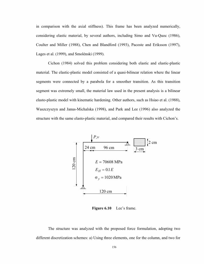
156

in comparison with the axial stiffness). This frame has been analyzed numerically,

considering elastic material, by several authors, including Simo and Vu-Quoc (1986),

Coulter and Miller (1988), Chen and Blandford (1993), Pacoste and Eriksson (1997),

Lages et al. (1999), and Smolénski (1999).

Cichon (1984) solved this problem considering both elastic and elastic-plastic

material. The elastic-plastic model consisted of a quasi-bilinear relation where the linear

segments were connected by a parabola for a smoother transition. As this transition

segment was extremely small, the material law used in the present analysis is a bilinear

elasto-plastic model with kinematic hardening. Other authors, such as Hsiao et al. (1988),

Waszczyszyn and Janus-Michalska (1998), and Park and Lee (1996) also analyzed the

structure with the same elasto-plastic material, and compared their results with Cichon’s.

E

E EH

y

=

=

=

70608

01

1020

MPa

MPa

.

σ

120

cm

P,v

120 cm

96 cm24 cm2 cm

3 cm

Figure 6.10 Lee’s frame.

The structure was analyzed with the proposed force formulation, adopting two

different discretization schemes: a) Using three elements, one for the column, and two for

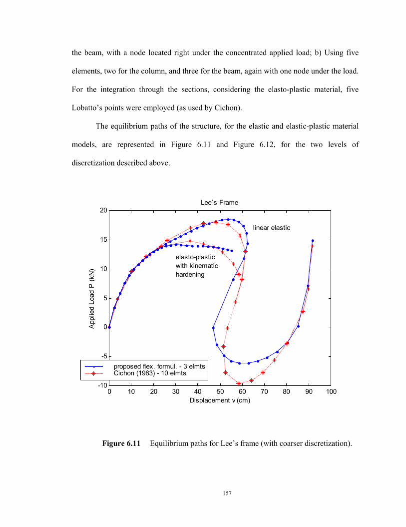
157

the beam, with a node located right under the concentrated applied load; b) Using five

elements, two for the column, and three for the beam, again with one node under the load.

For the integration through the sections, considering the elasto-plastic material, five

Lobatto’s points were employed (as used by Cichon).

The equilibrium paths of the structure, for the elastic and elastic-plastic material

models, are represented in Figure 6.11 and Figure 6.12, for the two levels of

discretization described above.

0 10 20 30 40 50 60 70 80 90 100-10

-5

0

5

10

15

20

linear elastic

elasto-plasticwith kinematichardening

Displacement v (cm)

App

lied

Load

P (k

N)

Lee`s Frame

proposed flex. formul. - 3 elmtsCichon (1983) - 10 elmts

Figure 6.11 Equilibrium paths for Lee’s frame (with coarser discretization).

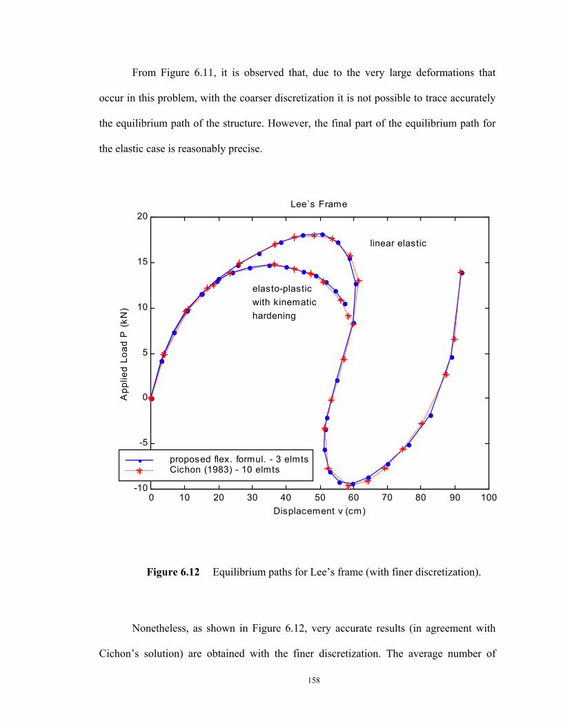
158

From Figure 6.11, it is observed that, due to the very large deformations that

occur in this problem, with the coarser discretization it is not possible to trace accurately

the equilibrium path of the structure. However, the final part of the equilibrium path for

the elastic case is reasonably precise.

0 10 20 30 40 50 60 70 80 90 100-10

-5

0

5

10

15

20

linear elastic

elasto-plasticwith kinematichardening

Lee`s Frame

Displacement v (cm)

App

lied

Load

P (

kN)

proposed flex. formul. - 3 elmtsCichon (1983) - 10 elmts

Figure 6.12 Equilibrium paths for Lee’s frame (with finer discretization).

Nonetheless, as shown in Figure 6.12, very accurate results (in agreement with

Cichon’s solution) are obtained with the finer discretization. The average number of

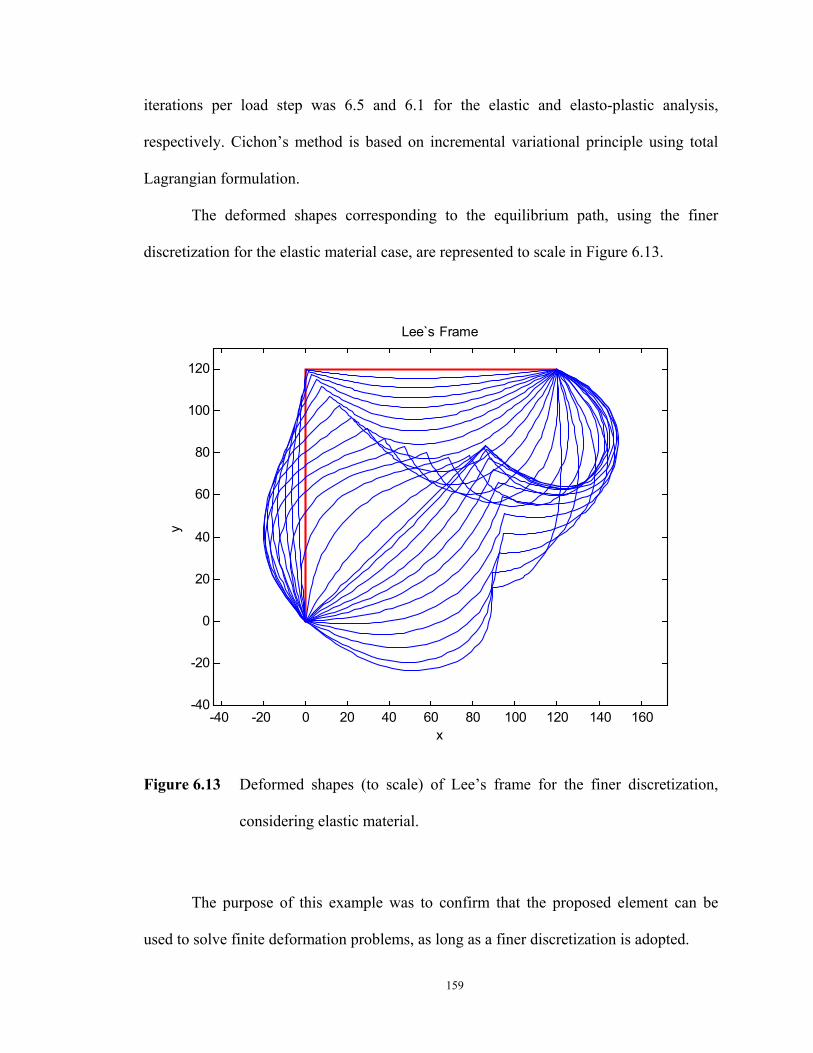
159

iterations per load step was 6.5 and 6.1 for the elastic and elasto-plastic analysis,

respectively. Cichon’s method is based on incremental variational principle using total

Lagrangian formulation.

The deformed shapes corresponding to the equilibrium path, using the finer

discretization for the elastic material case, are represented to scale in Figure 6.13.

-40 -20 0 20 40 60 80 100 120 140 160-40

-20

0

20

40

60

80

100

120

x

y

Lee`s Frame

Figure 6.13 Deformed shapes (to scale) of Lee’s frame for the finer discretization,

considering elastic material.

The purpose of this example was to confirm that the proposed element can be

used to solve finite deformation problems, as long as a finer discretization is adopted.

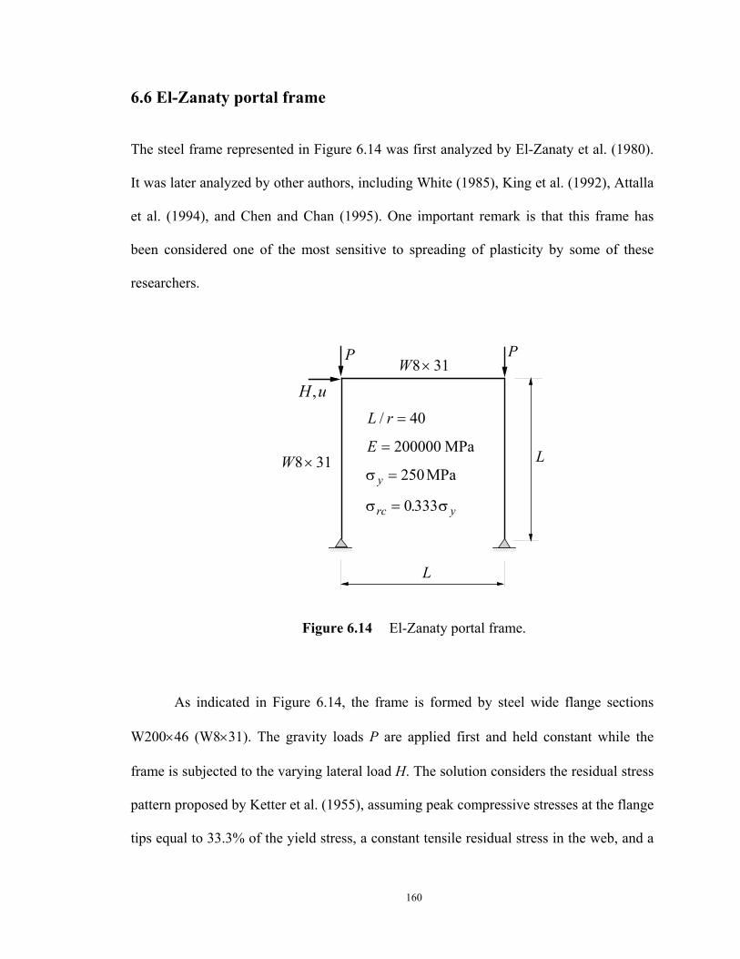
160

6.6 El-Zanaty portal frame

The steel frame represented in Figure 6.14 was first analyzed by El-Zanaty et al. (1980).

It was later analyzed by other authors, including White (1985), King et al. (1992), Attalla

et al. (1994), and Chen and Chan (1995). One important remark is that this frame has

been considered one of the most sensitive to spreading of plasticity by some of these

researchers.

L

P

L r

E

y

rc y

/

.

=

=

=

=

40

200000

250

0 333

MPa

MPaσ

σ σ

L

P

H u,

W8 31×

W8 31×

Figure 6.14 El-Zanaty portal frame.

As indicated in Figure 6.14, the frame is formed by steel wide flange sections

W200×46 (W8×31). The gravity loads P are applied first and held constant while the

frame is subjected to the varying lateral load H. The solution considers the residual stress

pattern proposed by Ketter et al. (1955), assuming peak compressive stresses at the flange

tips equal to 33.3% of the yield stress, a constant tensile residual stress in the web, and a

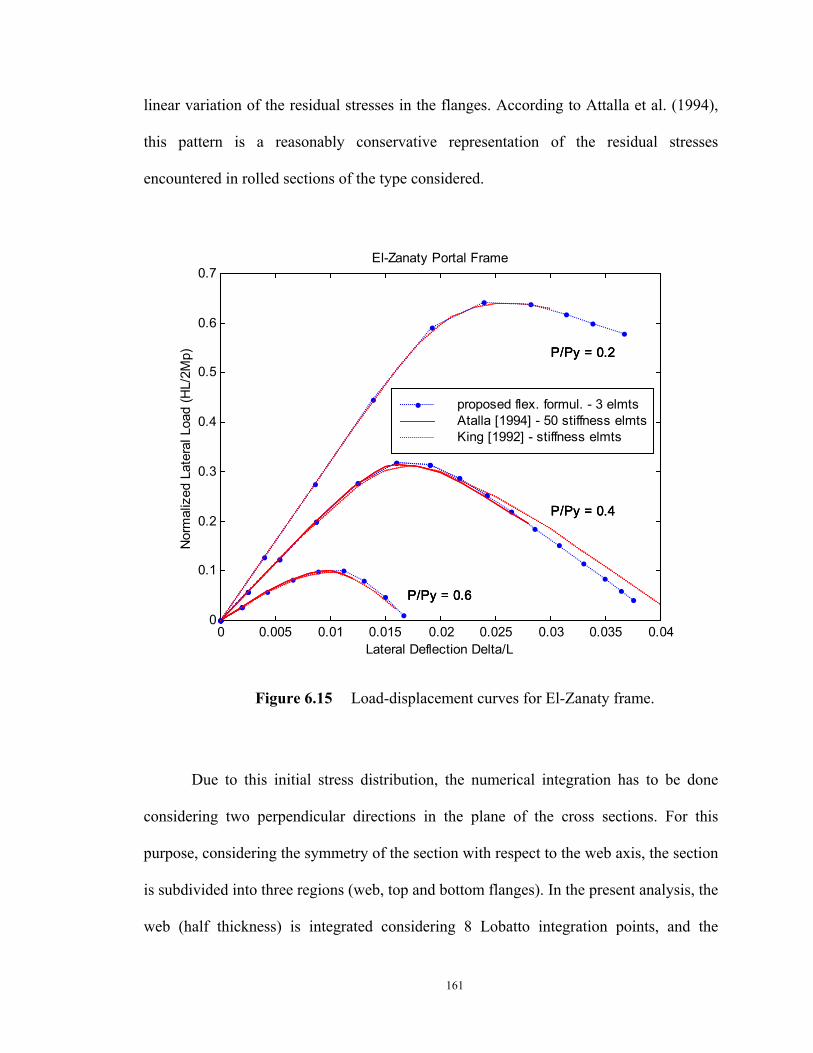
161

linear variation of the residual stresses in the flanges. According to Attalla et al. (1994),

this pattern is a reasonably conservative representation of the residual stresses

encountered in rolled sections of the type considered.

0 0.005 0.01 0.015 0.02 0.025 0.03 0.035 0.040

0.1

0.2

0.3

0.4

0.5

0.6

0.7

Lateral Deflection Delta/L

Nor

mal

ized

Lat

eral

Loa

d (H

L/2M

p)

P/Py = 0.6

P/Py = 0.4

P/Py = 0.2

El-Zanaty Portal Frame

P/Py = 0.6

P/Py = 0.4

P/Py = 0.2

P/Py = 0.6

P/Py = 0.4

P/Py = 0.2

proposed flex. formul. - 3 elmtsAtalla [1994] - 50 stiffness elmtsKing [1992] - stiffness elmts

Figure 6.15 Load-displacement curves for El-Zanaty frame.

Due to this initial stress distribution, the numerical integration has to be done

considering two perpendicular directions in the plane of the cross sections. For this

purpose, considering the symmetry of the section with respect to the web axis, the section

is subdivided into three regions (web, top and bottom flanges). In the present analysis, the

web (half thickness) is integrated considering 8 Lobatto integration points, and the

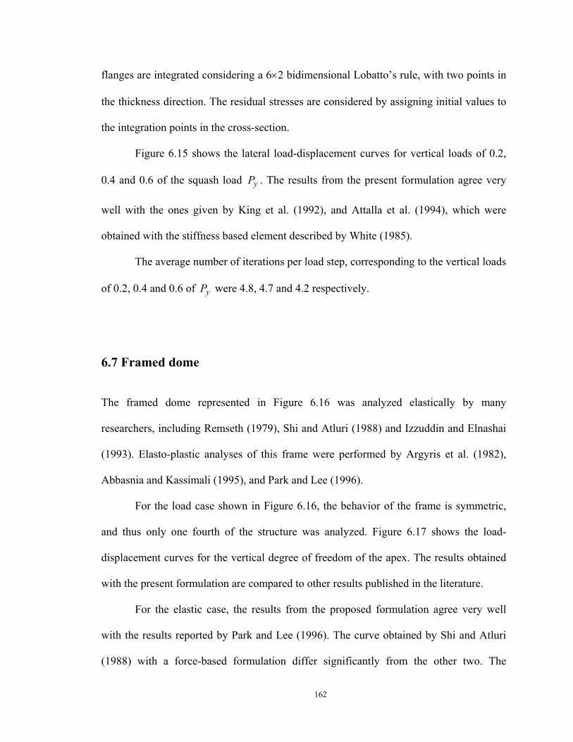
162

flanges are integrated considering a 6×2 bidimensional Lobatto’s rule, with two points in

the thickness direction. The residual stresses are considered by assigning initial values to

the integration points in the cross-section.

Figure 6.15 shows the lateral load-displacement curves for vertical loads of 0.2,

0.4 and 0.6 of the squash load yP . The results from the present formulation agree very

well with the ones given by King et al. (1992), and Attalla et al. (1994), which were

obtained with the stiffness based element described by White (1985).

The average number of iterations per load step, corresponding to the vertical loads

of 0.2, 0.4 and 0.6 of yP were 4.8, 4.7 and 4.2 respectively.

6.7 Framed dome

The framed dome represented in Figure 6.16 was analyzed elastically by many

researchers, including Remseth (1979), Shi and Atluri (1988) and Izzuddin and Elnashai

(1993). Elasto-plastic analyses of this frame were performed by Argyris et al. (1982),

Abbasnia and Kassimali (1995), and Park and Lee (1996).

For the load case shown in Figure 6.16, the behavior of the frame is symmetric,

and thus only one fourth of the structure was analyzed. Figure 6.17 shows the load-

displacement curves for the vertical degree of freedom of the apex. The results obtained

with the present formulation are compared to other results published in the literature.

For the elastic case, the results from the proposed formulation agree very well

with the results reported by Park and Lee (1996). The curve obtained by Shi and Atluri

(1988) with a force-based formulation differ significantly from the other two. The

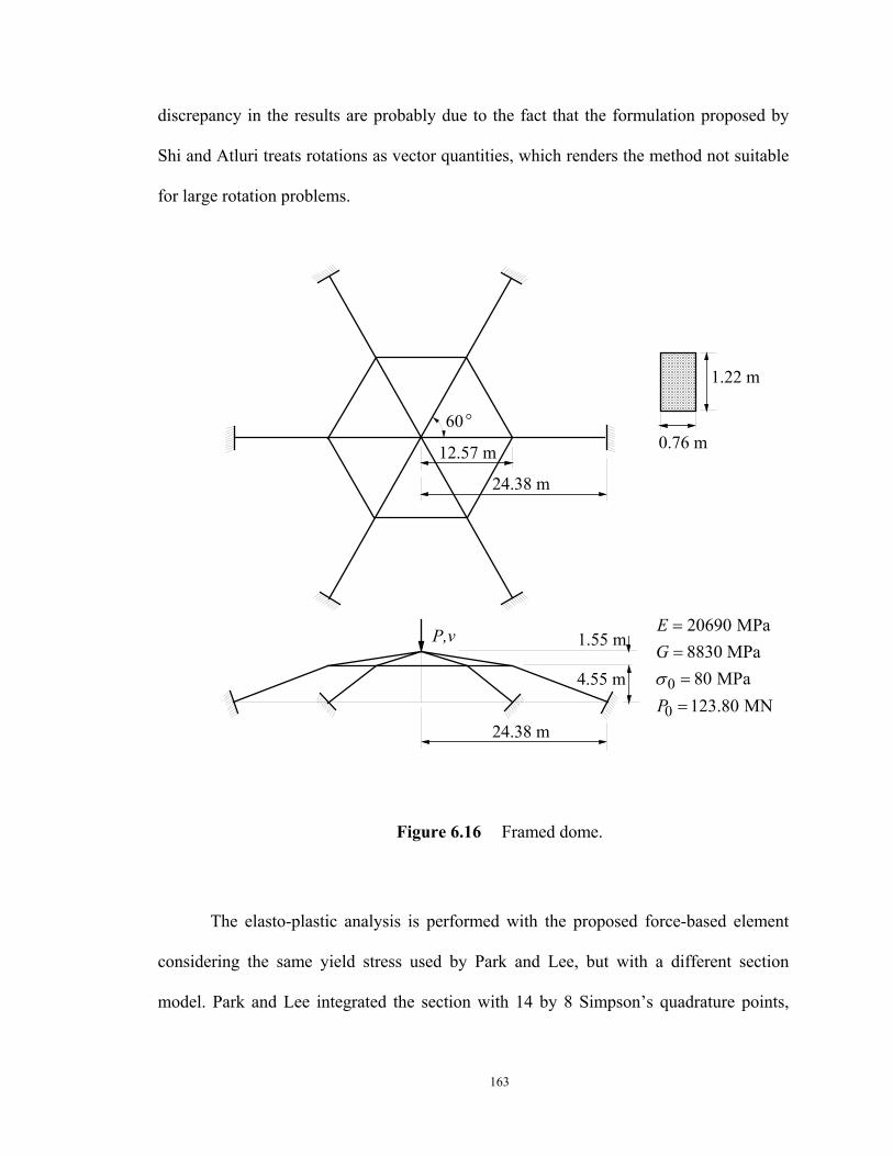
163

discrepancy in the results are probably due to the fact that the formulation proposed by

Shi and Atluri treats rotations as vector quantities, which renders the method not suitable

for large rotation problems.

P,v

0

0

20690 MPa8830 MPa80 MPa123.80 MN

EG

Pσ

====

1.22 m

0.76 m12.57 m

60

24.38 m

24.38 m

4.55 m

1.55 m

Figure 6.16 Framed dome.

The elasto-plastic analysis is performed with the proposed force-based element

considering the same yield stress used by Park and Lee, but with a different section

model. Park and Lee integrated the section with 14 by 8 Simpson’s quadrature points,

164

assuming the stress state given in eq. (4.43). In the present analysis the sections were

discretized with 40 by 10 fibers, assuming a uniaxial stress state and using the mid-point

rule in each fiber. The torsional behaviour was assumed linear.

0 0.5 1 1.5 2 2.5 3 3.5 4 4.50

0.2

0.4

0.6

0.8

1

1.2

Vertical displacement v (m)

Load

ratio

Framed dome

elastoplastic

elastic

Park (1996) - stiff. - 8 els./member Shi (1988) - flex. - 1 el./member Proposed flex. formul. - 1 el./member

Figure 6.17 Load-displacement curves for framed dome.

It is observed that the results agree well only up to a certain point on the curve,

which is probably explained by the different section behavior. It is important to mention,

however, that this structure was also analyzed with the proposed formulation using higher

integration orders and up to 6 elements per member, and it was observed that with just

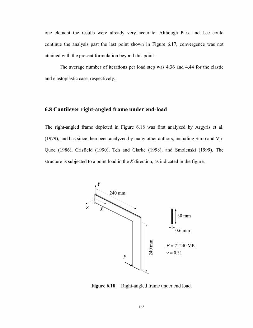
165

one element the results were already very accurate. Although Park and Lee could

continue the analysis past the last point shown in Figure 6.17, convergence was not

attained with the present formulation beyond this point.

The average number of iterations per load step was 4.36 and 4.44 for the elastic

and elastoplastic case, respectively.

6.8 Cantilever right-angled frame under end-load

The right-angled frame depicted in Figure 6.18 was first analyzed by Argyris et al.

(1979), and has since then been analyzed by many other authors, including Simo and Vu-

Quoc (1986), Crisfield (1990), Teh and Clarke (1998), and Smolénski (1999). The

structure is subjected to a point load in the X direction, as indicated in the figure.

71240 MPa0.31

Eν==24

0 m

m

Y

240 mm

30 mm

0.6 mm

Z X

P

Figure 6.18 Right-angled frame under end load.

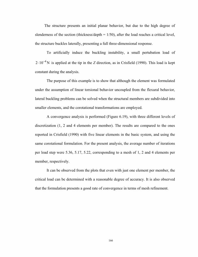
166

The structure presents an initial planar behavior, but due to the high degree of

slenderness of the section (thickness/depth = 1/50), after the load reaches a critical level,

the structure buckles laterally, presenting a full three-dimensional response.

To artificially induce the buckling instability, a small pertubation load of

42 10 N−⋅ is applied at the tip in the Z direction, as in Crisfield (1990). This load is kept

constant during the analysis.

The purpose of this example is to show that although the element was formulated

under the assumption of linear torsional behavior uncoupled from the flexural behavior,

lateral buckling problems can be solved when the structural members are subdivided into

smaller elements, and the corotational transformations are employed.

A convergence analysis is performed (Figure 6.19), with three different levels of

discretization (1, 2 and 4 elements per member). The results are compared to the ones

reported in Crisfield (1990) with five linear elements in the basic system, and using the

same corotational formulation. For the present analysis, the average number of iterations

per load step were 5.36, 5.17, 5.22, corresponding to a mesh of 1, 2 and 4 elements per

member, respectively.

It can be observed from the plots that even with just one element per member, the

critical load can be determined with a reasonable degree of accuracy. It is also observed

that the formulation presents a good rate of convergence in terms of mesh refinement.

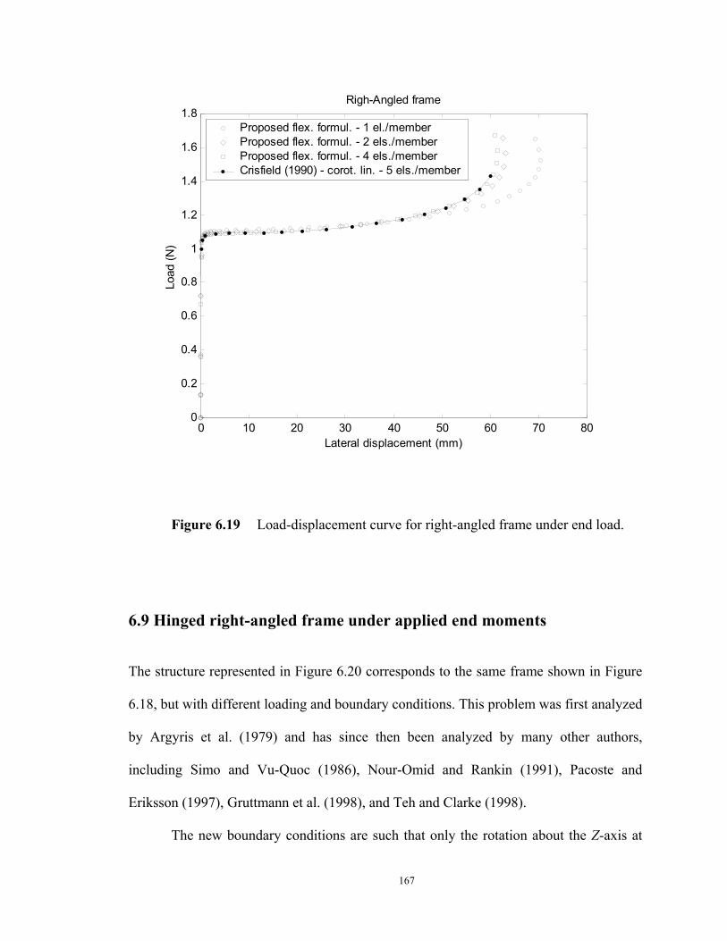
167

0 10 20 30 40 50 60 70 800

0.2

0.4

0.6

0.8

1

1.2

1.4

1.6

1.8Righ-Angled frame

Lateral displacement (mm)

Load

(N)

Proposed flex. formul. - 1 el./member Proposed flex. formul. - 2 els./member Proposed flex. formul. - 4 els./member Crisfield (1990) - corot. lin. - 5 els./member

Figure 6.19 Load-displacement curve for right-angled frame under end load.

6.9 Hinged right-angled frame under applied end moments

The structure represented in Figure 6.20 corresponds to the same frame shown in Figure

6.18, but with different loading and boundary conditions. This problem was first analyzed

by Argyris et al. (1979) and has since then been analyzed by many other authors,

including Simo and Vu-Quoc (1986), Nour-Omid and Rankin (1991), Pacoste and

Eriksson (1997), Gruttmann et al. (1998), and Teh and Clarke (1998).

The new boundary conditions are such that only the rotation about the Z-axis at

168

both ends, and the displacement in the X direction at the right support are allowed. The

structure is subjected to two opposing in-plane moments at the supports as indicated in

the figure. Due to the symmetry of the problem, only half of the frame needs to be

analyzed.

71240 MPa0.31

Eν==

240 mm

X

Y

30 mm

0.6 mm

M

240 mm

MZ

Figure 6.20 Right-angled frame under applied end moments.

As in the previous problem, the initial behavior of the structure is planar, until the

load reaches a critical level. At this point the stiffness matrix becomes singular and the

structure becomes unstable, presenting a sidesway (out-of-plane) buckling mode.

This problem presents extreme large three-dimensional rotations, and is a severe

test on the performance of the element. An interesting peculiarity of this problem is that

as the rotation of the hinged ends vary from 0 to 360 degrees, the top part of the frame

moves out of the plane, ‘rotates’ about the X axis and returns to the initial configuration.

After returning to the initial planar configuration, the applied end moment is the same in

magnitude but with reverse sign.

As pointed out by Simo and Vu-Quoc (1986), during the deformation process the

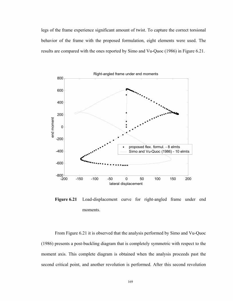
169

legs of the frame experience significant amount of twist. To capture the correct torsional

behavior of the frame with the proposed formulation, eight elements were used. The

results are compared with the ones reported by Simo and Vu-Quoc (1986) in Figure 6.21.

-200 -150 -100 -50 0 50 100 150 200-800

-600

-400

-200

0

200

400

600

800Right-angled frame under end moments

lateral displacement

end

mom

ent

proposed flex. formul. - 8 elmts Simo and Vu-Quoc (1986) - 10 elmts

Figure 6.21 Load-displacement curve for right-angled frame under end

moments.

From Figure 6.21 it is observed that the analysis performed by Simo and Vu-Quoc

(1986) presents a post-buckling diagram that is completely symmetric with respect to the

moment axis. This complete diagram is obtained when the analysis proceeds past the

second critical point, and another revolution is performed. After this second revolution

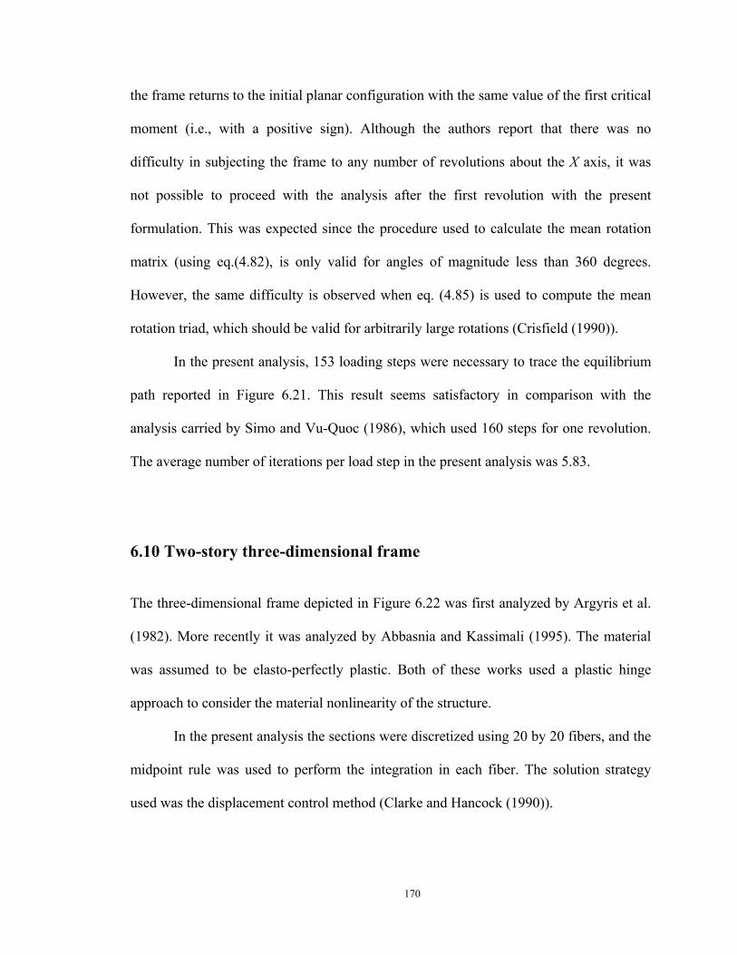
170

the frame returns to the initial planar configuration with the same value of the first critical

moment (i.e., with a positive sign). Although the authors report that there was no

difficulty in subjecting the frame to any number of revolutions about the X axis, it was

not possible to proceed with the analysis after the first revolution with the present

formulation. This was expected since the procedure used to calculate the mean rotation

matrix (using eq.(4.82), is only valid for angles of magnitude less than 360 degrees.

However, the same difficulty is observed when eq. (4.85) is used to compute the mean

rotation triad, which should be valid for arbitrarily large rotations (Crisfield (1990)).

In the present analysis, 153 loading steps were necessary to trace the equilibrium

path reported in Figure 6.21. This result seems satisfactory in comparison with the

analysis carried by Simo and Vu-Quoc (1986), which used 160 steps for one revolution.

The average number of iterations per load step in the present analysis was 5.83.

6.10 Two-story three-dimensional frame

The three-dimensional frame depicted in Figure 6.22 was first analyzed by Argyris et al.

(1982). More recently it was analyzed by Abbasnia and Kassimali (1995). The material

was assumed to be elasto-perfectly plastic. Both of these works used a plastic hinge

approach to consider the material nonlinearity of the structure.

In the present analysis the sections were discretized using 20 by 20 fibers, and the

midpoint rule was used to perform the integration in each fiber. The solution strategy

used was the displacement control method (Clarke and Hancock (1990)).

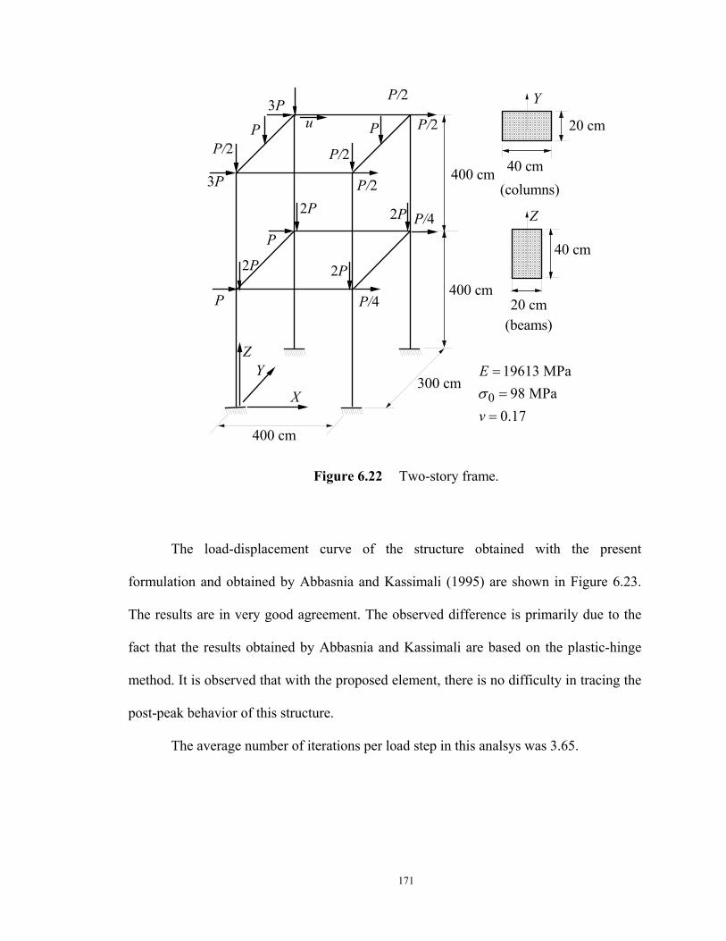
171

0

19613 MPa98 MPa

0.17

E

vσ==

=400 cm

300 cm

400 cm

3P

3P

P/2P

2P

P

P/2

P/2

P/2

P/2P

2P

2P

2P

P P/4

P/4

X

YZ

20 cm

40 cm(columns)

Y

40 cm

20 cm(beams)

Z

400 cm

u

Figure 6.22 Two-story frame.

The load-displacement curve of the structure obtained with the present

formulation and obtained by Abbasnia and Kassimali (1995) are shown in Figure 6.23.

The results are in very good agreement. The observed difference is primarily due to the

fact that the results obtained by Abbasnia and Kassimali are based on the plastic-hinge

method. It is observed that with the proposed element, there is no difficulty in tracing the

post-peak behavior of this structure.

The average number of iterations per load step in this analsys was 3.65.

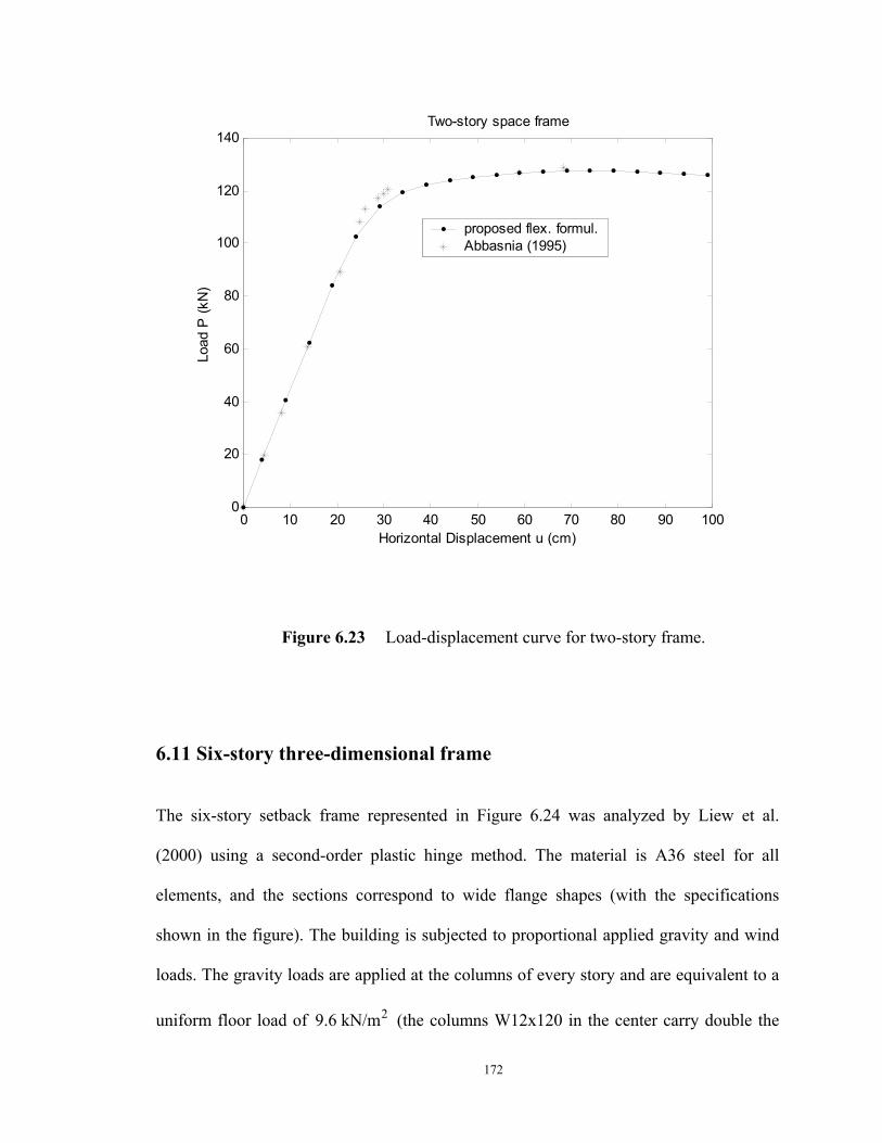
172

0 10 20 30 40 50 60 70 80 90 1000

20

40

60

80

100

120

140

Horizontal Displacement u (cm)

Load

P (k

N)

Two-story space frame

proposed flex. formul.Abbasnia (1995)

Figure 6.23 Load-displacement curve for two-story frame.

6.11 Six-story three-dimensional frame

The six-story setback frame represented in Figure 6.24 was analyzed by Liew et al.

(2000) using a second-order plastic hinge method. The material is A36 steel for all

elements, and the sections correspond to wide flange shapes (with the specifications

shown in the figure). The building is subjected to proportional applied gravity and wind

loads. The gravity loads are applied at the columns of every story and are equivalent to a

uniform floor load of 29.6 kN/m (the columns W12x120 in the center carry double the

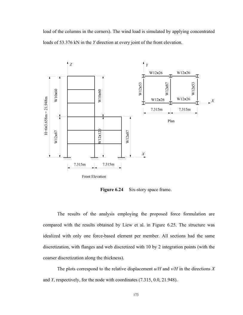
173

load of the columns in the corners). The wind load is simulated by applying concentrated

loads of 53.376 kN in the Y direction at every joint of the front elevation.

7.315m 7.315m

W12x26 W12x26

W12x26 W12x26

W12

x53

W12

x87

W12

x53

X

Y

Plan

7.315m 7.315m

W10

x60

W12

x87

W12

x120

X

Front Elevation

Z

W12

x87

W10

x60

H=6

x3.6

58m

= 2

1.94

8m

Figure 6.24 Six-story space frame.

The results of the analysis employing the proposed force formulation are

compared with the results obtained by Liew et al. in Figure 6.25. The structure was

idealized with only one force-based element per member. All sections had the same

discretization, with flanges and web discretized with 10 by 2 integration points (with the

coarser discretization along the thickness).

The plots correspond to the relative displacement u/H and v/H in the directions X

and Y, respectively, for the node with coordinates (7.315, 0.0, 21.948).

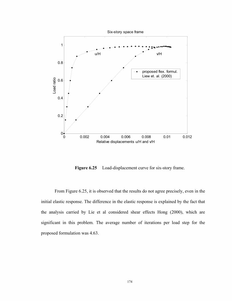
174

0 0.002 0.004 0.006 0.008 0.01 0.0120

0.2

0.4

0.6

0.8

1

Relative displacements u/H and v/H

Load

ratio

Six-story space frame

u/H v/H

proposed flex. formul.Liew et. al. (2000)

Figure 6.25 Load-displacement curve for six-story frame.

From Figure 6.25, it is observed that the results do not agree precisely, even in the

initial elastic response. The difference in the elastic response is explained by the fact that

the analysis carried by Lie et al considered shear effects Hong (2000), which are

significant in this problem. The average number of iterations per load step for the

proposed formulation was 4.63.

175

Chapter 7Conclusions

This study extended the planar force-based element with linear elastic material proposed

by Neuenhofer and Filippou (1998) to inelastic large displacement analysis. Both the

planar and spatial cases were developed in the present study trying to maintain the same

basic ideas of the original formulation.

The following conclusions can be drawn from the present study.

The basic equations of the problem, i.e., the compatibility and equilibrium

equations, used in the original work of Neuenhofer and Filippou (1998) were kept in the

present planar formulation. Consequently, the expression obtained for the flexibility

matrix is the same. However, a new derivation of the element formulation has been

presented in this work starting from the Hellinger-Reissner functional.

The formulation of the spatial element in the basic system corresponds to an

extension of the planar case (from uniaxial to biaxial bending). In the basic system, the

adopted kinematic assumptions led to linear torsional behavior geometrically uncoupled

from the flexural behavior. The section was assumed planar after deformation, such that

warping effects were neglected. Nonetheless, the flexure-torsion geometric coupling can

be accounted for, using the corotational formulation, as the structural members are

subdivided into smaller elements. This feature was specifically illustrated through

examples 6.7 and 6.8, where the lateral buckling behavior was captured correctly.

As in the original formulation, the CBDI (Curvature Based Displacement

176

Interpolation) procedure was used to determine the transverse displacements from the

curvature at the sample points. To compute the derivatives of the transverse

displacements with respect to the end forces, a new procedure was proposed to include

nonlinear material effects. Regarding the spatial case, although the transverse

displacements are obtained from the corresponding curvatures independently in each

direction, the determination of the derivatives of the displacements with respect to the

end forces is a coupled problem. The interaction is related to the coupled section behavior

(section stiffness) in the case of biaxial-bending in general inelastic sections.

Regarding the symmetry characteristic of the element flexibility matrix, it is

observed that, although the integrand in the expression of this flexibility matrix is non-

symmetric, a symmetric matrix is obtained when numerical integration is performed

using Gauss quadrature. When Gauss-Lobatto quadradure is employed the matrix tends to

be symmetric as the number of integration points increases. For other integration

methods, such as midpoint or trapezoidal rule, the flexibility matrix is non-symmetric

regardless of the number of integration points.

The symmetry property obtained with Gauss or Lobatto rules is probably related

to the use of the CBDI procedure and the orthogonality property of Legendre

polynomials, but this aspect of the formulation requires further study.

For the spatial case, since the global geometric stiffness matrix obtained with the

described corotational formulation is non-symmetric, the issue of symmetry of the

stiffness matrix in the basic system becomes moot. Nonetheless, a symmetric geometric

stiffness matrix could be obtained if other rotation parameters were used, as discussed,

for example, by Crisfield (1997), Ibrahimbegovic (1997), and Pacoste and Eriksson

177

(1997). In such a case, the symmetry of the basic stiffness matrix is relevant.

The described planar corotational formulation is exact, as no simplifications

related to the size of the nodal displacements and rotations are made. In the spatial case it

is usually considered that the nodal rotations are arbitrarily large, but that the difference

between them is small since the deformations along the element are considered moderate.

The spatial corotational formulation proposed by Crisfield (1990), based on this

assumption, was adopted in this work with some modifications.

The most important modification consists in the utilization of a different

expression for the mean rotation triad, which is simpler and allows for a consistent

computation of its variation. The adopted procedure to compute the mean rotation triad

is, however, limited to rotations of magnitude less than 360 degrees. This limitation is by

no means a severe restriction in practical civil engineering applications, and is reasonable

for a large range of other applications in structural mechanics. Nevertheless, for the

solution of other space problems subject to rotations larger than 360 degrees, the original

procedure proposed by Crisfield (1990) or any other corotational formulation that does

not impose this limitation can be used in conjunction with the present force-based

element.

The state determination procedures proposed in the present work have been

implemented in two general purpose finite element programs, FedeasLab and OpenSees4

which are based on the direct stiffness method. It has been observed (although not shown

in this study) that the iterative procedure provides quadratic convergence, while the non-

iterative approach converges slightly slower. However, for a small interval around the

4 http://millen.ce.berkeley.edu/index.html

178

equilibrium solution, the convergence rate of the non-iterative procedure is practically

quadratic.

It has been shown in the present study that the non-iterative state determination

can be constructed as a particularization of the iterative procedure, with the number of

local iterations equal to one.

The new algorithm can be viewed as a generalization of the state determination

procedures presented by Spacone et al. (1996b), and Neuenhofer and Filippou (1997) for

linear geometry/nonlinear material analysis, and the procedure described by Neuenhofer

and Filippou (1998) for linear material/nonlinear geometry.

The numerical examples shown in Chapter 6 demonstrated the accuracy and

efficiency of the proposed element. For most of the problems studied (Examples 1, 2, 3,

6, 7, 10 and 11), only one element per member was sufficient to obtain accurate results,

even in the presence of very large rotations (Examples 3 and 7).

The transformation matrices proposed in the original planar formulation by

Neuenhofer and Filippou (1998) were applicable to small rotations only. For instance,

when the original element was used to analyze the cantilever problem (Example 3), the

geometric nonlinear effect could not be captured, and the computed response was linear.

With exact transformations performed according to the described planar corotational

formulation, the overall improvement of the formulation was remarkable, and this

problem could be solved very accurately.

For problems with very large deformations along the element, as in Example 4,

the proposed formulation offered good results when the structural members were

subdivided into smaller elements.

179

Although the main motivation for the adoption of force-based elements is the

exactness in the treatment of nonlinear material behavior, some problems with linear

elastic material only (Examples 4, 8 and 9) were studied to demonstrate the capability of

the present element to solve problems in the large deformation range. The good results

are explained by the fact that by using the corotational formulation, as the structural

members are subdivided, the solution naturally approaches the solution provided by a

theory of finite strains, as observed by Pacoste and Eriksson (1997).

Recommendations for future research are:

a) Investigating the reason for the symmetry of the flexibility matrix obtained with

Gauss integration, and its possible connection with the orthogonality property of

Legendre polynomials.

b) Extending the formulation for dynamic analysis, through the derivation of a

consistent mass matrix.

c) Including shear effects.

d) Considering softening material behavior, with a procedure to avoid localization

problems.

e) Investigating the performance of the element to slender reinforced concrete

structures, subject to cyclic behavior.

f) Applying the formulation for problems of piles (with soil interaction) and beams on

elastic (or inelastic) foundation.

g) Extending the formulation to curved beams.

h) Extending the formulation to axisymetric shells.

180

i) Deriving a mixed beam element, where the forces are interpolated using the presented

force interpolation functions, and the displacements are interpolated independently,

using polynomial shape functions.

181

References

Abbasnia, R., and Kassimali, A. (1995). “Large deformation elastic-plastic analysis of

space frames.” J. Construct. Steel Research, 35, 275-290.

Aldstedt, E., and Bergan, P. G. (1978). “Nonlinear time-dependent concrete-frame

analysis.” J. Struct. Div., ASCE, 104(ST7), 1077-1092.

Alvarez, R. J., and Birnstiel, C. (1969). “Inelastic Analysis of Multistory Multibay

Frames.” J. Struct. Div., ASCE, 95(ST11), 2477-2503.

Argyris, J. (1982). “An excursion into large rotations.” Comput. Methods Appl. Mech.

Engrg., 32, 85-155.

Argyris, J. H., Balmer, H., Doltsinis, J. S., Dunne, P. C., Haase, M., Kleiber, M.,

Malejannakis, G. A., Mlejenek, J. P., Muller, M., and Scharpf, D. W. (1979).

“Finite element method - the natural approach.” Comput. Methods. Appl. Mech.

Engrg., 17/18, 1-106.

Argyris, J. H., Boni, B., Hindenlang, U., and Kleiber, M. (1982). “Finite element analysis

of two- and three-dimensional elasto-plastic frames - the natural approach.”

Comput. Methods Appl. Mech. Engrg., 35, 221-248.

Argyris, J. H., Kelsey, S., and Kamel, H. (1964). Matrix methods of structural analysis: a

precis of recent developments, Pergamon Press, Oxford.

Attalla, M. R., Deierlein, G. G., and McGuire, W. (1994). “Spread of plasticity: quasi-

plastic-hinge approach.” J. Struct. Engrg., ASCE, 120, 2451-2473.

Backlund, J. (1976). “Large deflection analysis of elasto-plastic beams and frames.” Int.

Journ. Mech. Science, 18, 269-277.

Barsan, G. M., and Chiorean, C. G. (1999). “Computer program for large deflection

elasto-plastic analysis of semi-rigid steel frameworks.” Comput. Struct., 72(699-

711).

Bathe, K. J. (1996). Finite Element Procedures, Prentice Hall, Englewood Cliffs, N. J.

182

Bathe, K.-J., and Bolourchi, S. (1979). “Large displacement analysis of three-

dimensional beam structures.” Int. J. Numer. Meth. Engng., 14, 961-986.

Belytschko, T., and Glaum, L. W. (1979). “Applications of higher order corotational

stretch theories to nonlinear finite element analysis.” Comput. Struct., 10, 175-

182.

Belytschko, T., and Hsieh, J. (1973). “Non-linear transient finite element analysis with

convected co-ordinates.” Int. J. Numer. Methods Engrg., 7, 255-271.

Burgoyne, C. J., and Crisfield, M. A. (1990). “Numerical integration strategy for plates

and shells.” Int. J. Numer. Methods Engrg., 29, 105-121.

Carol, I., and Murcia, J. (1989). “Nonlinear time-dependent analysis of planar frames

using an 'exact' formulation - I: Theory.” Comput. Struct, 33, 79-87.

Chan, S. L. (1988). “Geometric and material non-linear analysis of beam-columns and

frames using the minimum residual displacement method.” Int. J. Numer.

Methods Engrg., 26, 2657-2669.

Chebl, C., and Neale, K. W. (1984). “A finite element method for elastic-plastic beams

and columns at large deflections.” Comput. Struct, 18, 255-261.

Chen, H., and Blandford, G. E. (1993). “Work-increment-control method for nonlinear

analysis.” Int. J. Numer. Methods Engrg., 36, 909-930.

Chen, W. F., and Chan, S. L. (1995). “Second-order inelastic analysis of steel frames

using element with midspan and end springs.” J. Struct. Engrg., ASCE, 121, 530-

541.

Chen, W. F., and Liu, E. M. (1991). Stability design of steel frames, CRC Press, Boca

Raton, Fl.

Ciampi, V., and Carlesimo, L. (1986). “A nonlinear beam element for seismic analysis of

structures.” 8th European Conf. on Earthquake Engineering, Lisbon, Portugal.

Cichon, C. (1984). “Large displacements in-plane analysis of elastic-plastic frames.”

Comput. Struct, 19, 737-745.

Clarke, M. J., and Hancock, G. J. (1990). “A study of incremental-iterative strategies for

non-linear analyses.” Int. J. Numer. Methods Engrg., 29, 1365-1391.

183

Connor, J. J., Logchter, R. D., and Chan, S. C. (1968). “Nonlinear analysis of elastic

framed structures.” J. Struct. Div., ASCE, 94(ST6), 1525-1548.

Coulter, B. A., and Miller, R. E. (1988). “Numerical analysis of a generalized plane

'elastica' with non-linear material behaviour.” Int. J. Numer. Methods Engrg., 26,

617-630.

Crisfield, M. A. (1990). “A consistent co-rotational formulation for non-linear, three

dimensional beam elements.” Comput. Methods Appl. Mech. Engrg, 81, 131-150.

Crisfield, M. A. (1991). Non-linear Finite Element Analysis of Solids and Structures,

John Wiley & Sons, Chichester.

Crisfield, M. A. (1997). Non-linear finite element analysis of solids and structures -

Advanced topics, John Wiley & Sons, Chichester.

Crisfield, M. A., and Moita, G. F. (1996). “A unified co-rotational framework for solids,

shells and beams.” Int. J. for Solids & Structs., 33(20-22), 2969-2992.

El-Zanaty, M. H., and Murray, D. W. (1983). “Nonlinear finite element analysis of steel

frames.” J. Struct. Engrg., ASCE, 109, 353-369.

El-Zanaty, M. H., Murray, D. W., and Bjorhovde, R. (1980). “Inelastic behavior of

multistory steel frames.” Struct. Engrg. Rep. No. 83, Univ. of Alberta, Edmonton,

Alberta, Canada.

Frish-Fay, R. (1962). Flexible bars, Butterworths, London.

Gendy, A. S., and Saleeb, A. F. (1993). “Generalized yield surface representations in the

elasto-plastic three-dimensional analysis of frames.” Comput. Struct, 49(2), 351-

362.

Grubin, C. (1970). “Derivation of the quaternion scheme via the Euler axis and angle.”

Journal of Spacecraft and Rockets, 7, 1261-1263.

Gruttmann, F., Sauer, R., and Wagner, W. (1998). “A geometric nonlinear eccentric 3D-

beam element with arbitrary cross-sections.” Comput. Methods Appl. Mech.

Engrg., 160, 383-400.

Gummadi, L. N. B., and Palazotto, A. N. (1998). “Large strain analysis of beams and

arches undergoing large rotations.” Int. J. Non-Linear Mechanics, 33(4), 615-645.

184

Hong, C. (2000). “Private communication.” .

Hsiao, K. M., Hou, F. Y., and Spiliopoulos, K. V. (1988). “Large Displacement analysis

of elasto-plastic frames.” Comput. Struct, 28, 627-633.

Hsiao, K. M., Lin, J. Y., and Lin, W. Y. (1999). “A consistent co-rotational finite element

formulation for geometrically nonlinear dynamic analysis of 3-D beams.”

Comput. Methods Appl. Mech. Engrg., 169, 1-18.

Ibrahimbegovic, A. (1997). “On the choice of finite rotation parameters.” Comput.

Methods Appl. Mech. Engrg., 149, 49-71.

Iura, M. (1994). “Effects of coordinate system on the accuracy of corotational

formulation for Bernoulli-Euler's beam.” Int. J. Solids Structures, 31(20), 2793-

2806.

Izzuddin, B. A., and Elnashai, A. S. (1993). “Eulerian formulation for large-displacement

analysis of space frames.” J. Engrg. Mech., ASCE, 119(3), 549-569.

Jelenic, G., and Crisfield, M. A. (1998). “Interpolation of rotational variables in nonlinear

dynamics of 3d beams.” Int. J. Numer. Meth. Engng., 43, 1193-1222.

Jelenic, G., and Crisfield, M. A. (1999). “Geometrically exact 3D beam theory:

implementation of a strain-invariant finite element for statics and dynamics.”

Comput. Methods Appl. Mech. Engrg., 171, 141-171.

Jennings, A. (1968). “Frame analysis including change of geometry.” J. Struct. Div.,

ASCE, 94(ST3), 627-.

Jiang, J., and Olson, M. D. (1994). “Large elastic-plastic deformations of slender beams:

Co-rotational theory vs. von Karman theory.” Computational mechanics, 15, 117-

128.

Kam, T. Y. (1988). “Large deflection analysis of inelastic plane frames.” J. Struct.

Engrg., ASCE,, 114, 184-197.

Kassimali, A. (1983). “Large deformation analysis of elastic-plastic frames.” J. Struct.

Engrg., ASCE, 109, 1869-1887.

Ketter, R. L., Kaminsky, E. L., and Beedle, L. S. (1955). “Plastic deformation of wide-

flange beam columns.” Transactions ASCE, 120, 1028-1069.

185

King, W. S., and Chen, W. F. (1994). “Practical second-order inelastic analysis of

semirigid frames.” J. Struct. Engrg., ASCE, 120, 2156-2175.

King, W. S., White, D. W., and Chen, W. F. (1992). “Second-order inelastic analysis

methods for steel-frame design.” J. Struct. Engrg., ASCE, 118, 408-428.

Klumpp, A. R. (1976). “Singularity-free extraction of a quaternion from a direction-

cosine matrix.” Journal of Spacecraft and Rockets, 13(12), 754-755.

Kondoh, K., and Atluri, S. N. (1987). “Large-deformation, elasto-plastic analysis of

frames under nonconservative loading, using explicitly derived tangent stiffness

based on assumed stresses.” Computational Mechanics, 2, 1-25.

Kondoh, K., Tanaka, K., and Atluri, S. N. (1985). “An explicit expression for the tangent-

stiffness of a finitely deformed 3-d beam and its use in the analysis of space

frames.” Comput. Struct., 24(2), 253-271.

Korn, A., and Galambos, V. (1968). “Behavior of elastic-plastic frames.” Proc. ASCE,

94(ST5), 1119-1142.

Krenk, S., Vissing-Jorgensen, C., and Thesbjerg, L. (1999). “Efficient collapse analysis

for framed structures.” Comput. Struct., 72, 481-496.

Lages, E. N., Paulino, G. H., Menezes, I. F. M., and Silva, R. R. (1999). “Nonlinear finite

element analysis using an object-oriented philosophy - application to beam

elements and to the Cosserat continuum.” Engineering with Computers, 15, 73-

89.

Lee, S., Manuel, F. S., and Rossow, E. C. (1968). “Large deflections and stability of

elastic frames.” J. Engrg. Mech. Div., ASCE, EM2, 521-547.

Liew, J. Y. R., Chen, H., Shanmugam, N. E., and Chen, W. F. (2000). “Improved

nonlinear plastic hinge analysis of space frame structures.” Engineering

structures, 22, 1324-1338.

Liew, J. Y. R., White, D. W., and Chen, W. F. (1993). “Second order refined plastic-

hinge analysis for frame design. Part I.” J. Struct. Engrg., ASCE, 119, 3196-3216.

Lo, C. C., and Das Gupta, S. (1978). “Bending of a nonlinear rectangular beam in large

deflection.” J. Appl. Mech., ASME, 45, 213-214.

186

Marí, A. R., Esmond, C. C., and Scordelis, A. C. (1984). “Nonlinear material, geometric

and time dependent analysis of 3-d reinforced and prestressed concrete frames.”

Num. Meth. Non. Lin. Prob., Swansea, U. K, 339-352.

Mattiasson, K. (1981). “Numerical results from large deflection beam and frame

problems analyzed by means of elliptic integrals.” Int. J. Numer. Methods Engrg.,

17, 145-153.

Mattiasson, K., Bengtsson, A., and Samuelsson, A. (1985). “On the accuracy and

efficiency of numerical algorithms for geometrically nonlinear structural

analysis.” Finite Element Methods for Nonlinear Problems, Europe-US

Symposium, Trondheim, Norway.

Mattiasson, K., and Samuelsson, A. (1984). “Total and updated Lagrangian forms of the

co-rotational finite element formulation in geometrically and materially nonlinear

analysis.” Num. Meth. Non. Lin. Prob., Swansea, U. K, 134-151.

Meek, J. L., and Tan, H. S. (1984). “Geometrically nonlinear analysis of space frames by

an incremental iterative technique.” Comput. Methods Appl. Mechs. Engrg., 47,

261-262.

Meek, J. L., and Xue, Q. (1998). “A study on the instability problem for 3D frames.”

Comput. Methods Appl. Mech. Engrg, 158, 235-254.

Monti, G., and Spacone, E. (2000). “Reinforced Concrete fiber beam element with bond-

slip.” J. Struct. Engrg., 126(6), 654-661.

Nedergaard, H., and Pedersen, P. T. (1985). “Analysis procedure for space frames with

material and geometrical nonlinearities.” Finite Element Methods for Nonlinear

Problems, Europe-US Symposium, Trondheim, Norway, I-16-1 to I.16-20.

Neuenhofer, A., and Filippou, F. C. (1997). “Evaluation of nonlinear frame finite-element

models.” J. Struct. Engrg., ASCE, 123, 958-966.

Neuenhofer, A., and Filippou, F. C. (1998). “Geometrically nonlinear flexibility-based

frame finite element.” J. Struct. Engrg., ASCE, 124, 704-711.

Nour-Omid, B., and Rankin, C. C. (1991). “Finite rotation analysis and consistent

linearization using projectors.” Comput. Methods Appl. Mech. Engrg., 93, 353-

384.

187

Oran, C. (1973a). “Tangent Stiffness in plane frames.” J. Struct. Div., ASCE, 99(ST6),

973-985.

Oran, C. (1973b). “Tangent Stiffness in space frames.” J. Struct. Div., ASCE, 99(ST6),

987-1001.

Oran, C., and Kassimali, A. (1976). “Large deformations of framed structures under static

and dynamic loads.” Comput. Struct., 6(539-547).

Ovunc, B. A., and Ren, T. (1996). “Nonlinearities in the Analysis of Frames.” Comput.

Struct., 61(6), 1177-1184.

Pacoste, C., and Eriksson, A. (1997). “Beam elements in instability problems.” Comput.

Methods Appl. Mech. Engrg., 144(1-2), 163-197.

Park, M. S., and Lee, B. C. (1996). “Geometrically non-linear and elastoplastic three-

dimensional shear flexible beam element of Von-Mises-type hardening material.”

Int. J. Numer. Methods Engrg., 39(3), 383-408.

Petrangeli, M., and Ciampi, V. (1997). “Equilibrium based iterative solutions for the non-

linear beam problem.” Int. J. Numer. Methods Engrg., 40, 423-437.

Petrangeli, M., Pinto, P. E., and Ciampi, C. (1999). “Fiber element for cyclic bending and

shear of RC structures. I: Theory.” J. Engrg. Mech. , ASCE, 125(9), 994-1001.

Powell, G. H. (1969). “Theory of nonlinear elastic structures.” J. Struct. Div., ASCE,

95(ST12), 2687-1969.

Rankin, C. C., and Brogan, F. A. (1984). “An element-independent corotational

procedure for the treatment of large rotations.” Collapse analyses of structures,

ASME, New York, 85-100.

Ranzo, G., and Petrangeli, M. (1998). “A fibre finite beam element with section shear

modelling for seismic analysis of RC structures.” Journal of Earthquake

Engineering, 2(3), 443-473.

Reissner, E. (1972). “On one-dimensional finite-strain beam theory: The plane problem.”

J. Appl. Math. Phys (ZAMP), 23, 795-804.

Reissner, E. (1981). “On finite deformations of space-curved beams.” J. Appl. Math.

Phys (ZAMP), 32, 734-744.

188

Remseth, S. N. (1979). “Nonlinear static and dynamic analysis of framed structures.”

Comput. Struct., 10, 879-897.

Saje, M., Planinc, I., Turk, G., and Vratanar, B. (1997). “A kinematically exact finite

element formulation of planar elastic-plastic frames.” Comput. Methods Appl.

Mech. Engrg., 144, 125-151.

Schulz, M., and Filippou, F. C. (2000). “Curvature based spatial timoshenko beam

element for non-linear analysis.” Int. J. Numer. Methods Engrg., to appear.

Shi, G., and Atluri, S. N. (1988). “Elasto-plastic large deformation analysis of space-

frames: a plastic-hinge and stress-based explicit derivation of tangent stiffnesses.”

Int. J. Numer. Methods Engrg., 26, 589-615.

Simo, J. C. (1985). “A finite strain beam formulation. The three dimensional dynamic

problem: Part 1.” Comput. Methods Appl. Mech. Engrg, 49, 55-70.

Simo, J. C., Hjelmstad, K. D., and Taylor, R. L. (1984). “Numerical formulations for

finite deformation problems of beams accounting for the effect of trasverse

shear.” Comput. Methods Appl. Mech. Engrg., 42, 301-330.

Simo, J. C., and Taylor, R. L. (1985). “Consistent tangent operators for rate-independent

elastoplasticity.” Comput. Meths. Appl. Mech. Engrg., 48, 101-118.

Simo, J. C., and Vu-Quoc, L. (1986). “A three-dimensional finite strain rod model: Part

2: Computational aspects.” Comput. Methods Appl. Mech. Engrg., 58, 79-116.

Smolénski, W. M. (1999). “Statically and kinematically exact nonlinear theory of rods

and its numerical verification.” Comput. Methods Appl. Mech. Engrg., 178, 89-

113.

Spacone, E. (1994). “Flexibility-based finite element models for the nonlinear static and

dynamic analysis of concrete frame structures,” Ph.D., University of California at

Berkeley, Berkeley, CA.

Spacone, E., Ciampi, V., and Filippou, F. C. (1996a). “Mixed formulation of nonlinear

beam finite element.” Comput. Struct., 58, 71-83.

Spacone, E., Filippou, F. C., and Taucer, F. F. (1996b). “Fibre beam-column model for

non-linear analysis of R/C frames: Part I. Formulation.” Earthquake Eng. Struct.

Dyn., 25(711-725).

189

Spring, K. W. (1986). “Euler parameters and the use of quaternion algebra in the

manipulation of finite rotations: a review.” Mechanism and Machine Theory,

21(5), 365-373.

Spurrier, R. A. (1978). “Comment on singularity-free extraction of a quaternion from a

direction-cosine matrix.” Journal of Spacecraft and Rockets, 15(4), 255-256.

Teh, L. H., and Clarke, M. J. (1998). “Co-rotational and Lagrangian formulations for

elastic three-dimensional beam finite elements.” Journal of Constructional Steel

Research, 48, 123-144.

Timoshenko, S. P., and Woinowsky-Krieger, S. (1959). Theory of plates and shells,

McGraw-Hill.

Tuomala, M. T. E., and Mikkola, M. J. (1984). “Comparative study on the nonlinear

response of plane frames and arches.” Num. Meth. Non. Lin. Prob., Swansea, U.

K, 203-214.

Waszczyszyn, Z., and Janus-Michalska, M. (1998). “Numerical approach to the 'exact'

finite element analysis of in-plane finite displacements of framed structures.”

Comput. Struct., 69, 525-535.

White, D. W. (1985). “Material and geometric nonlinear analysis of local planar behavior

in steel frames using interactive computer graphics,” MS, Cornell Univ., Ithaca,

N.Y.

Williams, F. W. (1964). “An Approach to the non-linear behaviour of the members of a

rigid jointed plane framework with finite deflections.” Quart. Journ. Mech. and

Applied Math, 17(Pt. 4), 451-469.

Wood, R. D., and Zienkiewicz, O. C. (1977). “Geometrically nonlinear finite element

analysis of beams, frames, arches, and axisymmetric shells.” Comput. Struct., 7,

725-735.

Ziemian, R. D., McGuire, W., and Deierlein, G. G. (1992). “Inelastic limit states design.

Part I: Planar frame studies.” J. Struct. Engrg., ASCE, 118(2532-2549).

190

Appendix ADerivation of the CBDI Influence Matrix

The first step for the derivation of the CBDI influence matrix consists in interpolating the

curvature field ( )κ ξ in terms of curvature values ( )j jκ κ ξ= at integration points jξ

1( ) ( ) ,

n

j jj

xlL

κ ξ ξ κ ξ=

= =∑ (A.1)

where ( )jl ξ are Lagrangian polynomials

1,

1,

( )

( )( )

n

ii i j

j n

j ii i j

l

ξ ξ

ξξ ξ

= ≠

= ≠

−

=−

∏

∏(A.2)

The transverse displacement v(x) is determined from the kinematic relation

( ) ( )x v xκ ′′= , i.e., the function v(x) is obtained integrating the curvature field ( )xκ twice

2( ) ( )d d ( )d dv x x x x Lκ κ ξ ξ ξ = = ∫ ∫ ∫ ∫ (A.3)

It should be noted that ( ) ( ( ))x xκ κ ξ= is used as an abuse of notation. Similarly,

the same applies for the function ( )( ) ( )v x v xξ= .

The Lagrangian polynomials given in eq. (A.2) can be more conveniently

integrated using the relation

2 11( ) ( ) 1 n

nl lξ ξ ξ ξ ξ − −= 1G (A.4)

191

where G is the so-called Vandermode matrix

2 11 1 1

2 1

1

1

n

nn n n

ξ ξ ξ

ξ ξ ξ

−

−

=

G (A.5)

which depends only on the number and location of the integration points iξ , 1, ,i n= … .

From eqs. (A.1), (A.3) and (A.4), the displacements are obtained as

2 3 12

1 2( )2 6 ( 1)

nv x L c c

n nξ ξ ξ ξ

+−

= + + +

1G κ (A.6)

The integration constants 1c and 2c are determined using the boundary conditions

(0) ( ) 0v v L= = (see Figure 2.4). Thus,

21

2

1 1 12 6 ( 1)

0

c Ln n

c

−= −+

=

1G κ(A.7)

The expression for the displacement v(x) can be written as

2 2 3 1

2 2

1

1 1 1( ) ( ) ( ) ( )2 6 ( 1)

( ) ( )

n

n

j jj

v x Ln n

L l L

ξ ξ ξ ξ ξ ξ

ξ κ ξ

+ −

=

= − − −+

= =∑

1G κ

l κ(A.8)

where

2 3 11 1 1( ) ( ) ( ) ( )2 6 ( 1)

n

n nξ ξ ξ ξ ξ ξ ξ+ −= − − −

+1l G (A.9)

is the row vector of n integrated Lagrangian polynomials, including the integration

constant 1c .

192

Evaluation of the displacements v at the integration points iξ leads to

2 *

1 1( ) ( ) 1, ,

n n

i i j i j ij jj j

v v L l l i nξ ξ κ κ= =

= = = =∑ ∑ … (A.10)

where the term

* 2 ( )ij j il L l ξ= (A.11)

is the CBDI influence matrix

2 3 11 1 1 1 1 1

* 2

2 3 1

1 1 1( ) ( ) ( )2 6 ( 1)

1 1 1( ) ( ) ( )2 6 ( 1)

n

nn n n n n n

n nL

n n

ξ ξ ξ ξ ξ ξ

ξ ξ ξ ξ ξ ξ

+

−

+

− − − + =

− − − +

1l G (A.12)

such that

*=v l κ (A.13)

193

Appendix BRotation of a Triad via the Smallest Rotation

This appendix presents the derivation of the expressions given in Section 3.7, for rotating

a triad 1 2 3[ ]=P p p p such that one of its unit vectors, say 1p , coincides with another

independent unit vector, say 1e , via the smallest possible rotation.

The expression for the rotation matrix was obtained in Section 3.7 and is repeated

here for convenience.

1 1 1 1 1 1T1 1

1( ) ( ) ( )1

= + × + × ×+

R I S p e S p e S p ep e

(B.1)

The triad 1 2 3[ ]=E e e e is determined by rotating the triad P with the rotation

matrix R given in eq. (B.1)

1 2 3 1 2 3[ ] [ ]= = =E e e e R p p p RP (B.2)

such that each unit vector ip can be rotated onto ie as

1 1 1 1 1 1T1 1

1( ) ( ) ( )1

i i i i i= = + × + × ×+

e Rp p S p e p S p e S p e pp e

(B.3)

In order to simplify this equation, the following identity can be used

T T( ) ( ) ( ) ( )× = × × = −S a b c a b c a c b b c a (B.4)

such that

T T1 1 1 1 1 1 1 1( ) ( ) ( )i i i i× = × × = −S p e p p e p p p e e p p (B.5)

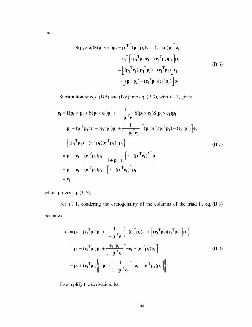
194

and

T T T1 1 1 1 1 1 1 1 1 1

T T T1 1 1 1 1 1

T T T1 1 1 1 1

T T T1 1 1 1 1

( ) ( ) ( ) ( )

( ) ( )

( )( ) ( )

( ) ( )( )

i i i

i i

i i

i i

× × = − − −

= − − −

S p e S p e p p p p e e p p e

e p p e e p p p

p e p p e p e

p p e p e p p

(B.6)

Substitution of eqs. (B.5) and (B.6) into eq. (B.3), with 1i = , gives

1 1 1 1 1 1 1 1 1 1 1T1 1

T T T T T1 1 1 1 1 1 1 1 1 1 1 1 1 1T

1 1

T T T1 1 1 1 1 1 1

T T 21 1 1 1 1 1 1 1T

1 1T T

1 1 1 1 1 1

1( ) ( ) ( )1

1( ) ( ) ( )( ) ( )1

( ) ( )( )

1( ) 1 ( )1

( ) 1 (

= = + × + × ×+

= + − + − +

− −

= + − − − +

= + − − −

e Rp p S p e p S p e S p e pp e

p p p e e p p p e p p e p ep e

p p e p e p p

p e e p p p e pp e

p e e p p p 1 1

1

)

=

e p

e

(B.7)

which proves eq. (3.76).

For 1i ≠ , condering the orthogonality of the columns of the triad P, eq. (B.3)

becomes

T T T T1 1 1 1 1 1 1 1T

1 1T

T T11 1 1 1 1 1T

1 1

T T1 1 1 1 1 1T

1 1

1( ) ( ) ( )( )1

( ) ( )1

1( ) ( )1

i i i i i

ii i

i i

= − + − + +

= − + − + +

= + − + − + +

e p e p p e p e e p e p pp e

e pp e p p e e p pp e

p e p p e e p pp e

(B.8)

To simplify the derivation, let

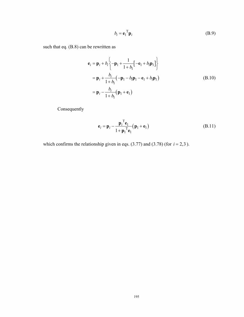
195

T1i ib = e p (B.9)

such that eq. (B.8) can be rewritten as

[ ]

( )

( )

1 1 1 11

1 1 1 1 1 11

1 11

11

1

1

i i i

ii

ii

b bb

b b bb

bb

= + − + − +

+

= + − − − ++

= − ++

e p p e p

p p p e p

p p e

(B.10)

Consequently

( )T

11 1T

1 11i

i i= − ++

p ee p p ep e

(B.11)

which confirms the relationship given in eqs. (3.77) and (3.78) (for 2,3i = ).

196

Appendix CDerivation of the Spatial Geometric Stiffness Matrix

This appendix presents a detailed derivation of the spatial geometric stiffness matrix,

related to the inclusion of rigid body modes in the transformation from the basic to the

global coordinate system.

The geometric stiffness matrix is given by eq. (4.127) being repeated here for

convenience

T:ˆG

∂=

∂TK PD

(C.1)

such that

6T

1

ˆs s G

sPδ δ δ

== =∑T P t K D (C.2)

where sδ t are the variations of the rows of matrix T. Thus, the geometric stiffness matrix

is easily obtained by taking the variations of each row st and multiplying the result by

the corresponding basic forces sP .

It is convenient to rewrite the final expression for the geometric stiffness matrix

as a summation of several matrices, such that

G A B C D E F= + + + + +K K K K K K K (C.3)

The first term AK is obtained by taking the variation of eq. (4.115), and

considering eq. (4.108)

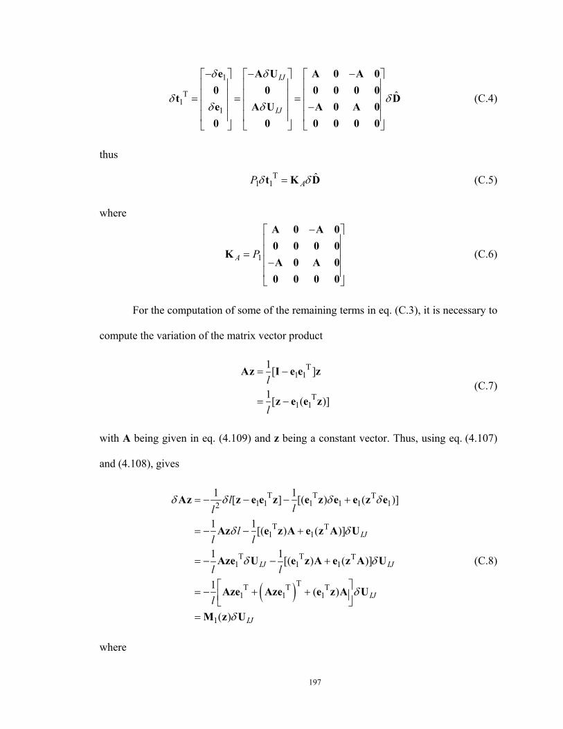
197

1

T1

1

ˆ

IJ

IJ

δ δ

δ δδ δ

− − − = = = −

e A U A 0 A 00 0 0 0 0 0

t De A U A 0 A 00 0 0 0 0 0

(C.4)

thus

T1 1

ˆAPδ δ=t K D (C.5)

where

1A P

− = −

A 0 A 00 0 0 0

KA 0 A 00 0 0 0

(C.6)

For the computation of some of the remaining terms in eq. (C.3), it is necessary to

compute the variation of the matrix vector product

T1 1

T1 1

1[ ]

1[ ( )]

l

l

= −

= −

Az I e e z

z e e z(C.7)

with A being given in eq. (4.109) and z being a constant vector. Thus, using eq. (4.107)

and (4.108), gives

( )

T T T1 1 1 1 1 12

T T1 1

T T T1 1 1

TT T T1 1 1

1

1 1[ ] [( ) ( )]

1 1[( ) ( )]

1 1[( ) ( )]

1 ( )

( )

IJ

IJ IJ

IJ

IJ

lll

ll l

l l

l

δ δ δ δ

δ δ

δ δ

δ

δ

= − − − +

= − − +

= − − +

= − + + =

Az z e e z e z e e z e

Az e z A e z A U

Aze U e z A e z A U

Aze Aze e z A U

M z U

(C.8)

where

198

( )TT T T1 1 1 1

1( ) ( )l = − + +

M z Aze Aze A e z (C.9)

is a symmetric matrix.

It is also necessary to compute the variation of the matrix vector product

T T1 1 1 1

1( ) ( )2k k k = + + L r z r e Az Ar e r z (C.10)

with 1( )kL r being given in eq. (4.112), and z being a constant vector. Thus

( ) ( )( )

( ) ( )

T T T1 1 1 1

T T1 1 1 1

T TT T1 1 1 1

TT T1 1 1 1

1( ) ( ) ( ) ( )2

( ) ( )

1 ( )2

( ) ( )

k k k k

k k k

k k k

k k k

δ δ δ δ

δ δ δ δ

δ δ

δ δ δ

= + +

+ + + + +

= + + + +

+ + + +

L r z Az e r Az r e r e Az

Ar z e r e r z Ar A r

Azr Ar z e Aze e r zA r

Ar z r r e Az e r z Ar

(C.11)

Substitution of eqs. (4.106), (4.108), and (C.8) into eq. (C.11) gives

( )( )( )

T TT T1 1 1 1 1 1

T T T1 1 1 1

1( ) ( ) ( ) ( )21 ( ) ( ) ( ) ( )4

k k k k k IJ

k k k I J

δ δ

δ δ

= + + + +

− + + + +

L r z Azr A Ar z A r e M z e r zM r U

Aze S r e r zAS r Ar z S r γ γ(C.12)

which can be rewritten in matrix form as

1 11 12 11 12ˆ( ) ( , ) ( , ) ( , ) ( , )k k k k kδ δ = − L r z g r z g r z g r z g r z D (C.13)

where

( )( )

T TT T11 1 1 1 1 1

T T T12 1 1 1 1

1( , ) ( ) ( ) ( )21( , ) ( ) ( ) ( ) ( )4

k k k k k

k k k k

= − + + + +

= − + + +

g r z Azr A Ar z A r e M z e r zM r

g r z Aze S r e r zAS r Ar z S r(C.14)

It is also necessary to compute the variation of the product

199

( )T T2 1 1 1 1 1

1( ) 2 ( ) ( ) ( ) ( ) ( )4k k k k = − − + L r z S r z r e S r z S r e e r z (C.15)

with 1( )kL r being given in eq. (4.112), and z being a constant vector. Thus,

( ) ( )( )

( )( )

T T T2 1 1 1 1 1

T T1 1 1 1 1 1

T1 1 1

T T T1 1 1 1 1

T T1 1 1

1 1

1( ) 2 ( ) ( ) ( ) ( ) ( )4

( ) ( ) ( ) ( )

( ) ( )

1 ( ) ( ) ( ) ( )4

( ) ( ) ( )

2 ( ) ( )

k k k k k

k k

k

k k k

k k

δ δ δ δ δ

δ δ

δ δ

δ

δ

= − − +

− + − +

− +

= − + + +

+ −

+ − −

L r z S r z r e S r z S r z r e e r

e r z S r e e r z S r e

S r e z e r

S r zr e r zS r S r e z e

r e S z S r e z r

S z S r ze( )( )(

)( )

T T1 1 1

T T T1 1 1 1

T T1 1 1 1

T T1 1 1 1 1

( ) ( )

1 ( ) ( ) ( ) ( )41 ( ) ( ) ( ) ( ) ( ) 2 ( ) ( )8

( ) ( ) ( ) ( ) ( )

k

k k k IJ

k k k

k k I J

δ

δ

δ δ

+ +

= − + + +

+ − + +

+ − + +

e r zS e r

S r zr A e r zS r A S r e z A U

r e S z S r S r e z S r S z S r

S r ze S r e r zS e S r γ γ (C.16)

which can be rewritten as

2 21 22 21 22ˆ( ) ( , ) ( , ) ( , ) ( , )k k k k kδ δ = − L r z g r z g r z g r z g r z D (C.17)

where

( )(

)

T T T21 1 1 1 1

T T22 1 1 1 1

T T1 1 1 1 1

1( , ) ( ) ( ) ( ) ( )41( , ) ( ) ( ) ( ) ( ) ( ) 2 ( ) ( )8

( ) ( ) ( ) ( ) ( )

k k k k

k k k k

k k

= + + +

= − + +

+ − +

g r z S r zr A e r zS r A S r e z A

g r z r e S z S r S r e z S r S z S r

S r ze S r e r zS e S r

(C.18)

From eq. (4.111) the variation of the product ( )kL r z is

200

1

2

1

2

( )( ) ˆ( ) ( , )( )( )

k

kk k

k

k

δδ

δ δδδ

= = −

L r zL r z

L r z G r z DL r z

L r z

(C.19)

where

11 12 11 12

21 22 21 22

11 12 11 12

21 22 21 22

ˆ( , )k δ

− − = − − − −

g g g gg g g g

G r z Dg g g g

g g g g

(C.20)

It is observed that

T21 12( , ) ( , )k k=g r z g r z (C.21)

and that the matrix 11( , )kg r z is symmetric. However, due to the non-symmetry of matrix

22( , )kg r z , the matrix ( , )kG r z is non-symmetric.

The variation of the second row of matrix T is obtained from the first of eqs.

(4.123)

T2 2 1 3 3 3

3

2 21 1 33

T2 2 2 23 1 1 3

3

1 ( ) tan2cos

1 ( ) ( )2cos

1ˆtan ( ) ( )2cos

I I I II

I I II

I I I II

δ δθ θθ

δ δ δθ

θ δ δ δ δθ

= +

+ + +

= + + +

t L r n h

L r n L r n h

t t D L r n L r n h

(C.22)

The variation of the remaining rows are computed in a similar maner, and result

in

201

T T3 3 3 2 23 1 1 3

3

T T4 4 4 3 32 1 1 2

2

T T5 5 5 3 32 1 1 2

2

T T6 6 61

1

1ˆtan ( ) ( )2cos

1ˆtan ( ) ( )2cos

1ˆtan ( ) ( )2cos

1ˆtan (2cos

J J J JJ

I I I II

J J J JJ

J J JJ

δ θ δ δ δθ

δ θ δ δ δθ

δ θ δ δ δθ

δ θ δθ

= + + +

= + − − −

= + − − −

= +

t t t D L r n L r n h

t t t D L r n L r n h

t t t D L r n L r n h

t t t D L r3 32 2

2 23 3 1

T6 6 3 31 2 2

1

2 23 3 1

) ( )

( ) ( )

1ˆtan ( ) ( )2cos

( ) ( )

J J

J J J

I I II II

I I I

δ

δ δ δ

θ δ δθ

δ δ δ

+

− − +

− − +

− − +

n L r n

L r n L r n h

t t D L r n L r n

L r n L r n h

(C.23)

where

T6 3 22 3 1

1

T6 3 22 3 1

1

1 ( ) ( )2cos

1 ( ) ( )2cos

J J JJJ

I I III

θ

θ

= − +

= − +

t L r n L r n h

t L r n L r n h(C.24)

Matrix BK corresponds to the summation of terms such as T2 23tan Iθ t t in eqs.

(C.22) and (C.23), resulting in

T T T2 2 2 3 3 3 4 4 43 23

T T T5 5 5 6 6 6 6 612 1

tan tan tan

tan ( tan tan )

B I J I

J I JI I I J J

P P P

P P

θ θ θ

θ θ θ

= + +

+ + − +

K t t t t t t

t t t t t t(C.25)

For the description of the remaining matrices, it is useful to define the following

‘scaled’ basic forces

2 3 42 3 4

3 23

5 6 65 6 6

12 1

2cos 2cos 2cos

2cos 2cos 2cos

I J I

I JJ I J

P P Pm m m

P P Pm m m

θ θ θ

θ θ θ

= = =

= = =(C.26)

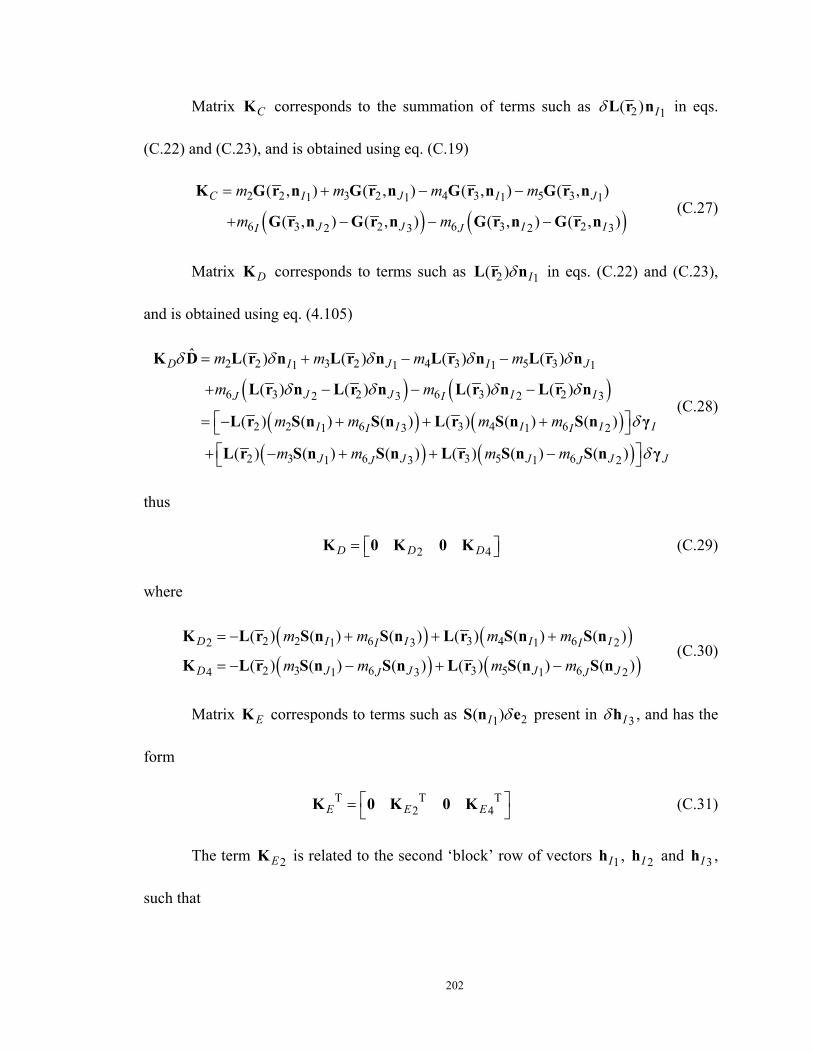
202

Matrix CK corresponds to the summation of terms such as 2 1( ) IδL r n in eqs.

(C.22) and (C.23), and is obtained using eq. (C.19)

( ) ( )2 2 3 2 4 3 5 31 11 1

6 3 2 6 3 22 32 3

( , ) ( , ) ( , ) ( , )

( , ) ( , ) ( , ) ( , )

C I J I J

J J I II J

m m m m

m m

= + − −

+ − − −

K G r n G r n G r n G r n

G r n G r n G r n G r n(C.27)

Matrix DK corresponds to terms such as 2 1( ) IδL r n in eqs. (C.22) and (C.23),

and is obtained using eq. (4.105)

( ) ( )( ) ( )( )

2 2 3 2 4 3 5 31 11 1

6 3 2 6 3 22 32 3

2 2 6 3 4 61 3 1 2

2 3 6 3 5 61 3 1

ˆ ( ) ( ) ( ) ( )

( ) ( ) ( ) ( )

( ) ( ) ( ) ( ) ( ) ( )

( ) ( ) ( ) ( ) ( ) (

D I J I J

J J I IJ I

I I I I II I

J J JJ J

m m m m

m m

m m m m

m m m m

δ δ δ δ δ

δ δ δ δ

δ

= + − −

+ − − −

= − + + +

+ − + + −

K D L r n L r n L r n L r n

L r n L r n L r n L r n

L r S n S n L r S n S n γ

L r S n S n L r S n S( )2)J Jδ n γ

(C.28)

thus

2 4D D D= K 0 K 0 K (C.29)

where

( ) ( )( ) ( )

2 2 6 3 4 62 1 3 1 2

2 3 6 3 5 64 1 3 1 2

( ) ( ) ( ) ( ) ( ) ( )

( ) ( ) ( ) ( ) ( ) ( )D I I I II I

D J J J JJ J

m m m m

m m m m

= − + + +

= − − + −

K L r S n S n L r S n S n

K L r S n S n L r S n S n(C.30)

Matrix EK corresponds to terms such as 21( )I δS n e present in 3Iδh , and has the

form

T T T2 4E E E = K 0 K 0 K (C.31)

The term 2EK is related to the second ‘block’ row of vectors 1Ih , 2Ih and 3Ih ,

such that

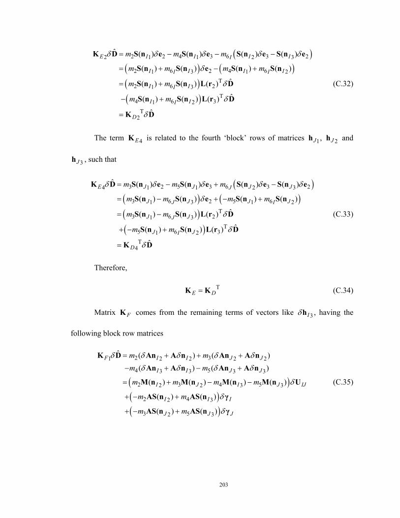
203

( )( ) ( )( )( )

2 2 4 3 6 3 22 1 1 2 3

2 6 2 4 61 3 1 2T

2 6 21 3T

4 6 31 2T

2

ˆ ( ) ( ) ( ) ( )

( ) ( ) ( ) ( )

ˆ( ) ( ) ( )

ˆ( ) ( ) ( )

ˆ

E I I I II

I I I II I

I II

I II

D

m m m

m m m m

m m

m m

δ δ δ δ δ

δ

δ

δ

δ

= − − −

= + − +

= +

− +

=

K D S n e S n e S n e S n e

S n S n e S n S n

S n S n L r D

S n S n L r D

K D

(C.32)

The term 4EK is related to the fourth ‘block’ rows of matrices 1Jh , 2Jh and

3Jh , such that

( )( ) ( )( )( )

3 2 5 3 6 3 24 1 1 2 3

3 6 2 5 61 3 1 2T

3 6 21 3T

5 6 31 2T

4

ˆ ( ) ( ) ( ) ( )

( ) ( ) ( ) ( )

ˆ( ) ( ) ( )

ˆ( ) ( ) ( )

ˆ

E J J J JJ

J J J JJ I

J JJ

J JI

D

m m m

m m m m

m m

m m

δ δ δ δ δ

δ

δ

δ

δ

= − + −

= − + − +

= −

+ − +

=

K D S n e S n e S n e S n e

S n S n e S n S n

S n S n L r D

S n S n L r D

K D

(C.33)

Therefore,

TE D=K K (C.34)

Matrix FK comes from the remaining terms of vectors like 3Iδh , having the

following block row matrices

( )( )( )

2 31 2 2 2 2

4 53 3 3 3

2 3 4 52 32 3

2 42 3

3 52 3

ˆ ( ) ( )( ) ( )

( ) ( ) ( ) ( )

( ) ( )

( ) ( )

F I I J J

I I J J

I J I J IJ

I I I

J J J

m mm m

m m m m

m m

m m

δ δ δ δ δδ δ δ δ

δ

δ

δ

= + + +

− + − +

= + − −

+ − +

+ − +

K D An A n An A nAn A n An A n

M n M n M n M n U

AS n AS n γ

AS n AS n γ

(C.35)

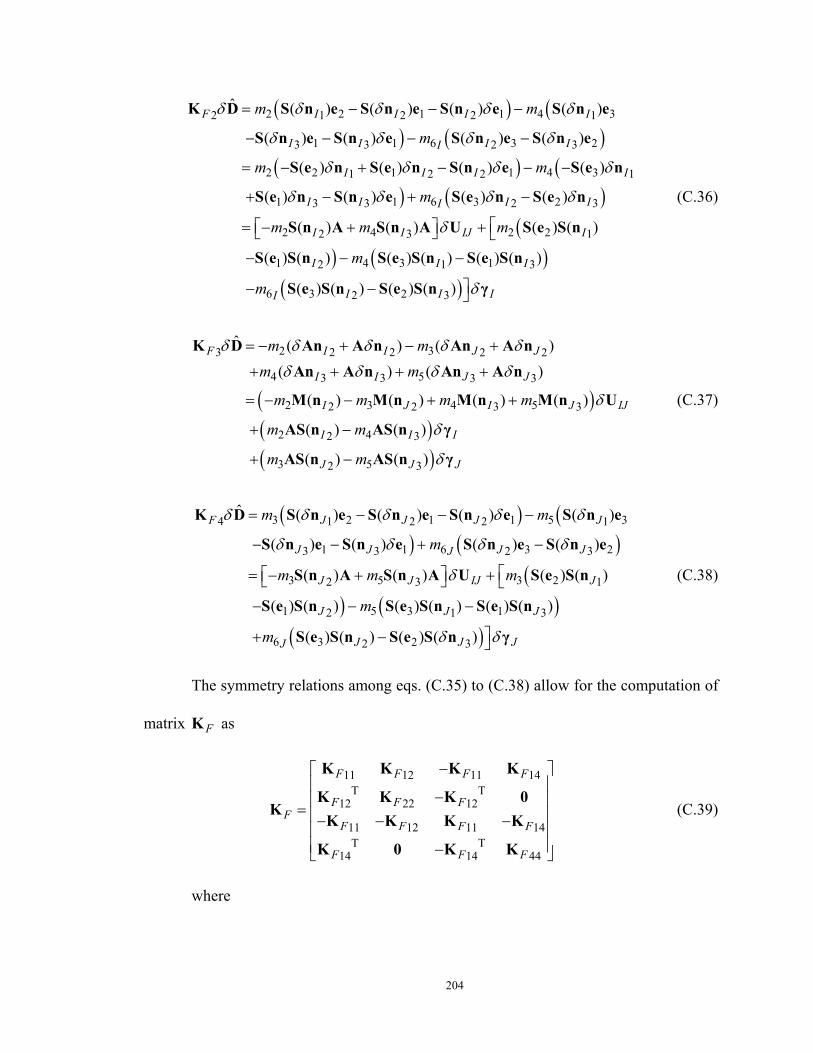
204

( ) () ( )

( ) () ( )

2 2 1 1 4 32 1 2 2 1

1 1 6 3 23 3 2 3

2 2 1 1 4 31 2 2 1

1 1 6 3 23 3 2 3

2 42

ˆ ( ) ( ) ( ) ( )

( ) ( ) ( ) ( )

( ) ( ) ( ) ( )

( ) ( ) ( ) ( )

( ) (

F I I I I

I I I II

I I I I

I I I II

I I

m m

m

m m

m

m m

δ δ δ δ δ

δ δ δ δ

δ δ δ δ

δ δ δ δ

= − − −

− − − −

= − + − − −

+ − + −

= − +

K D S n e S n e S n e S n e

S n e S n e S n e S n e

S e n S e n S n e S e n

S e n S n e S e n S e n

S n A S n () ( )

( )

2 23 1

1 4 3 12 1 3

6 3 22 3

) ( ) ( )

( ) ( ) ( ) ( ) ( ) ( )

( ) ( ) ( ) ( )

IJ I

I I I

I I II

m

m

m

δ

δ

+ − − −

− −

A U S e S n

S e S n S e S n S e S n

S e S n S e S n γ

(C.36)

( )( )( )

2 33 2 2 2 2

4 53 3 3 3

2 3 4 52 32 3

2 42 3

3 52 3

ˆ ( ) ( )( ) ( )

( ) ( ) ( ) ( )

( ) ( )

( ) ( )

F I I J J

I I J J

I J I J IJ

I I I

J J J

m mm m

m m m m

m m

m m

δ δ δ δ δδ δ δ δ

δ

δ

δ

= − + − +

+ + + +

= − − + +

+ −

+ −

K D An A n An A nAn A n An A n

M n M n M n M n U

AS n AS n γ

AS n AS n γ

(C.37)

( ) () ( )

() ( )

3 2 1 1 5 34 1 2 2 1

1 1 6 3 23 3 2 3

3 5 3 22 3 1

1 5 3 12 1 3

6 3 22

ˆ ( ) ( ) ( ) ( )

( ) ( ) ( ) ( )

( ) ( ) ( ) ( )

( ) ( ) ( ) ( ) ( ) ( )

( ) ( ) ( ) (

F J J J J

J J J JJ

J J IJ J

J J J

JJ

m m

m

m m m

m

m

δ δ δ δ δ

δ δ δ δ

δ

δ

= − − −

− − + −

= − + + − − −

+ −

K D S n e S n e S n e S n e

S n e S n e S n e S n e

S n A S n A U S e S n

S e S n S e S n S e S n

S e S n S e S( )3)J Jδn γ

(C.38)

The symmetry relations among eqs. (C.35) to (C.38) allow for the computation of

matrix FK as

11 12 11 14T T

12 22 12

11 12 11 14T T

14 14 44

F F F F

F F FF

F F F F

F F F

−

− = − − − −

K K K K

K K K 0K

K K K K

K 0 K K

(C.39)

where

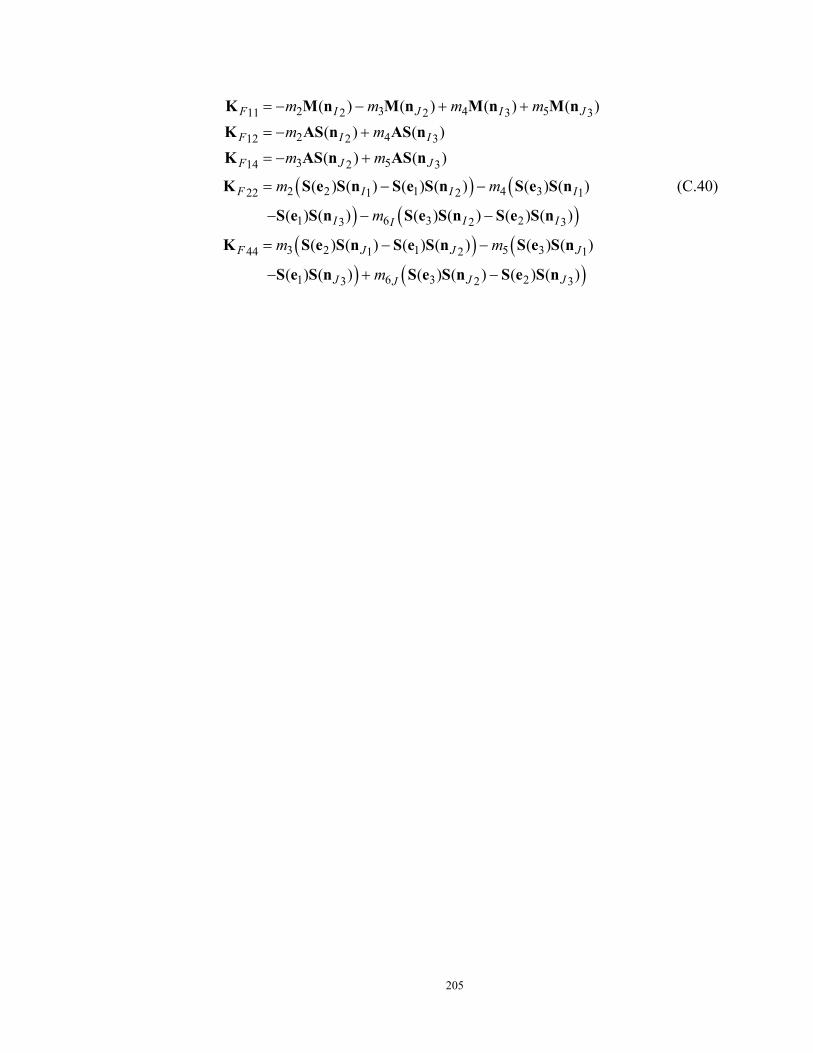
205

( ) () ( )

2 3 4 511 2 32 3

2 412 2 3

3 514 2 3

2 2 1 4 322 1 2 1

1 6 3 23 2 3

3 2 144 1

( ) ( ) ( ) ( )( ) ( )( ) ( )

( ) ( ) ( ) ( ) ( ) ( )

( ) ( ) ( ) ( ) ( ) ( )

( ) ( ) ( ) (

F I J I J

F I I

F J J

F I I I

I I II

F J

m m m mm mm m

m m

m

m

= − − + +

= − +

= − +

= − −

− − −

= −

K M n M n M n M nK AS n AS nK AS n AS n

K S e S n S e S n S e S n

S e S n S e S n S e S n

K S e S n S e S( ) () ( )

5 32 1

1 6 3 23 2 3

) ( ) ( )

( ) ( ) ( ) ( ) ( ) ( )J J

J J JJ

m

m

−

− + −

n S e S n

S e S n S e S n S e S n

(C.40)