Discretization

Pieter Abbeel UC Berkeley EECS

TexPoint fonts used in EMF. Read the TexPoint manual before you delete this box.: AAAAAAAAAAA

[Drawing from Sutton and Barto, Reinforcement Learning: An Introduction, 1998]

Markov Decision Process

Assumption: agent gets to observe the state

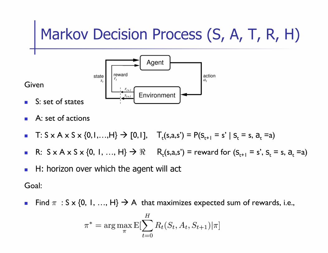
Markov Decision Process (S, A, T, R, H)

Given

n  S: set of states

n  A: set of actions

n  T: S x A x S x {0,1,…,H} à [0,1], Tt(s,a,s’) = P(st+1 = s’ | st = s, at =a)

n  R: S x A x S x {0, 1, …, H} à < Rt(s,a,s’) = reward for (st+1 = s’, st = s, at =a)

n  H: horizon over which the agent will act

Goal:

n  Find ¼ : S x {0, 1, …, H} à A that maximizes expected sum of rewards, i.e.,

Value Iteration n  Algorithm:

n  Start with for all s.

n  For i=1, … , H For all states s 2 S:

This is called a value update or Bellman update/back-up

n  = the expected sum of rewards accumulated when starting from state s and acting optimally for a horizon of i steps

n  = the optimal action when in state s and getting to act for a horizon of i steps

n  S = continuous set

n  Value iteration becomes impractical as it requires to compute, for all states s 2 S:

Continuous State Spaces

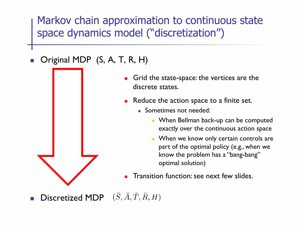
Markov chain approximation to continuous state space dynamics model (“discretization”)

n  Original MDP (S, A, T, R, H)

n  Discretized MDP

n  Grid the state-space: the vertices are the discrete states.

n  Reduce the action space to a finite set. n  Sometimes not needed:

n  When Bellman back-up can be computed exactly over the continuous action space

n  When we know only certain controls are part of the optimal policy (e.g., when we know the problem has a “bang-bang” optimal solution)

n  Transition function: see next few slides.

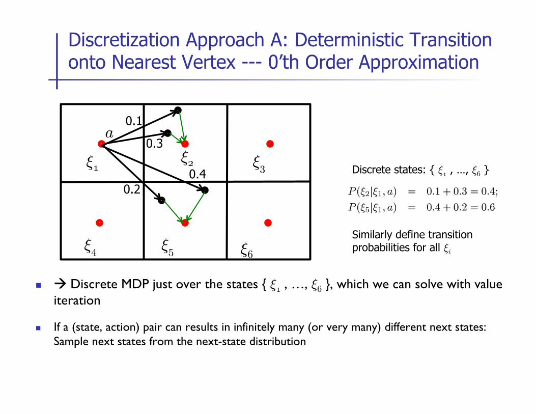
Discretization Approach A: Deterministic Transition onto Nearest Vertex --- 0’th Order Approximation

Discrete states: { »1 , …, »6 } Similarly define transition probabilities for all »i

»1

»5 »4

»3 »2

»6

a

n  à Discrete MDP just over the states { »1 , …, »6 }, which we can solve with value iteration

n  If a (state, action) pair can results in infinitely many (or very many) different next states: Sample next states from the next-state distribution

0.1

0.3

0.4 0.2

Discretization Approach B: Stochastic Transition onto Neighboring Vertices --- 1’st Order Approximation

Discrete states: { »1 , …, »12 }

n  If stochastic: Repeat procedure to account for all possible transitions and weight accordingly

n  Need not be triangular, but could use other ways to select neighbors that contribute. “Kuhn triangulation” is particular choice that allows for efficient computation of the weights pA, pB, pC, also in higher dimensions

»1

»5

»9 »10 »11 »12

»8

»4 »3 »2

»6 »7

s’ a

Discretization: Our Status

n  Have seen two ways to turn a continuous state-space MDP into a discrete state-space MDP

n  When we solve the discrete state-space MDP, we find:

n  Policy and value function for the discrete states

n  They are optimal for the discrete MDP, but typically not for the original MDP

n  Remaining questions:

n  How to act when in a state that is not in the discrete states set?

n  How close to optimal are the obtained policy and value function?

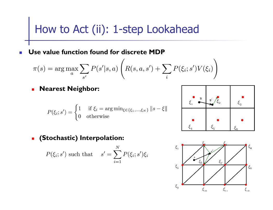
n  For non-discrete state s choose action based on policy in nearby states

n  Nearest Neighbor:

n  (Stochastic) Interpolation:

How to Act (i): 0-step Lookahead

n  Use value function found for discrete MDP

n  Nearest Neighbor:

n  (Stochastic) Interpolation:

How to Act (ii): 1-step Lookahead

n  Think about how you could do this for n-step lookahead

n  Why might large n not be practical in most cases?

How to Act (iii): n-step Lookahead

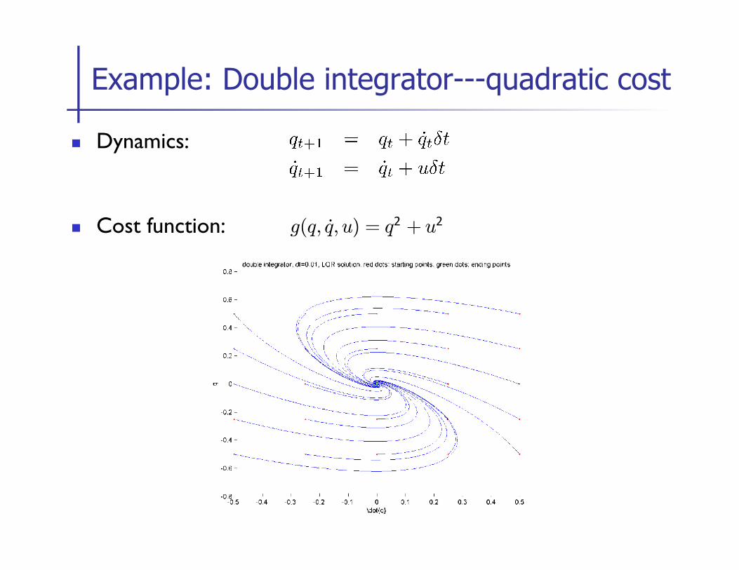
n  Dynamics:

n  Cost function:

Example: Double integrator---quadratic cost

g(q, q̇, u) = q2 + u2

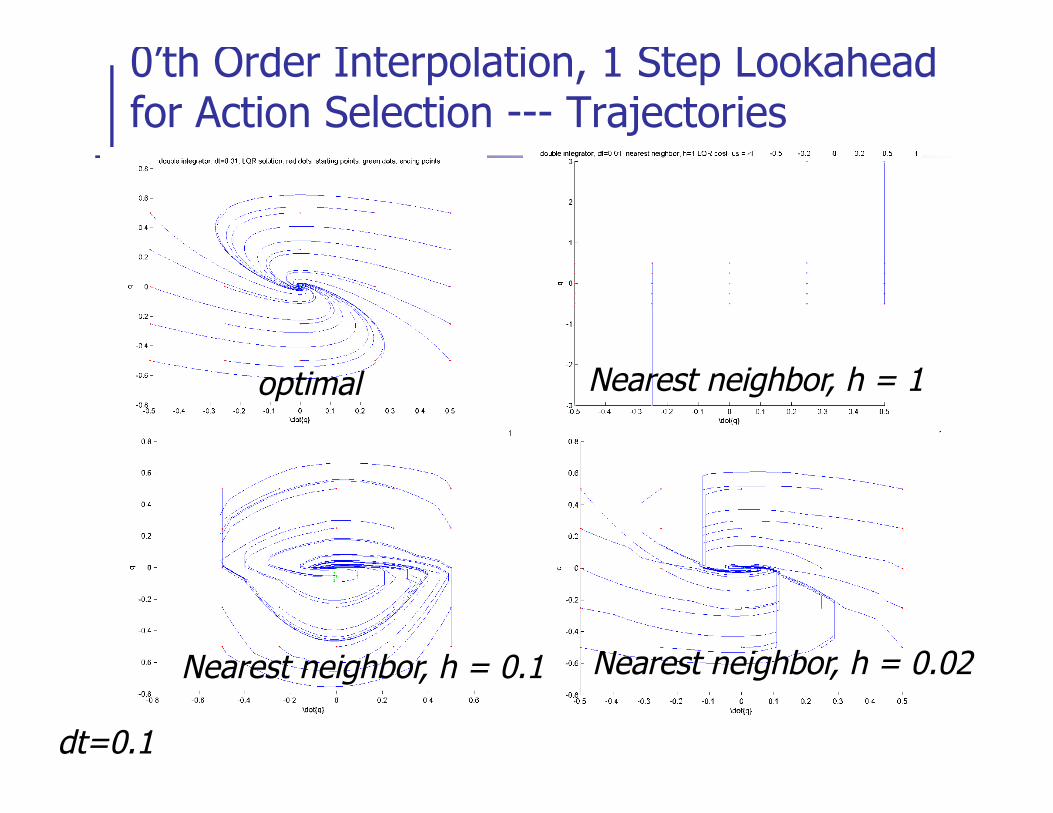
0’th Order Interpolation, 1 Step Lookahead for Action Selection --- Trajectories

optimal Nearest neighbor, h = 1

Nearest neighbor, h = 0.02 Nearest neighbor, h = 0.1

dt=0.1

0’th Order Interpolation, 1 Step Lookahead for Action Selection --- Resulting Cost

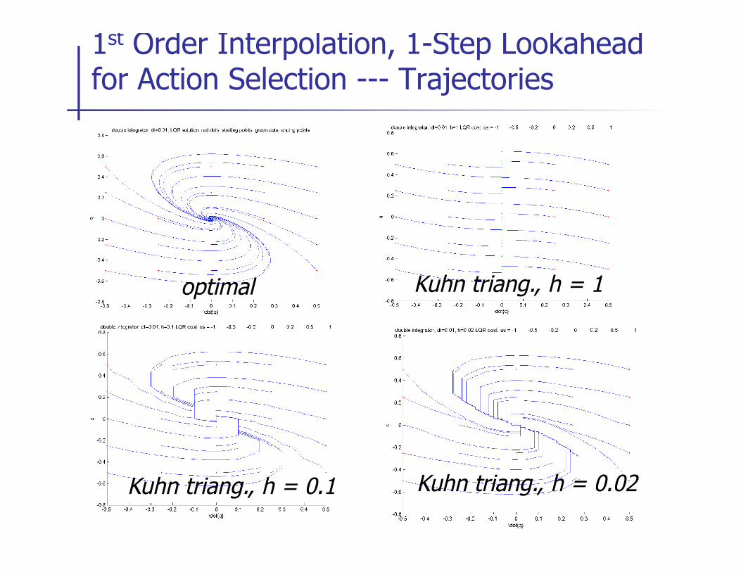
1st Order Interpolation, 1-Step Lookahead for Action Selection --- Trajectories

optimal Kuhn triang., h = 1

Kuhn triang., h = 0.02 Kuhn triang., h = 0.1

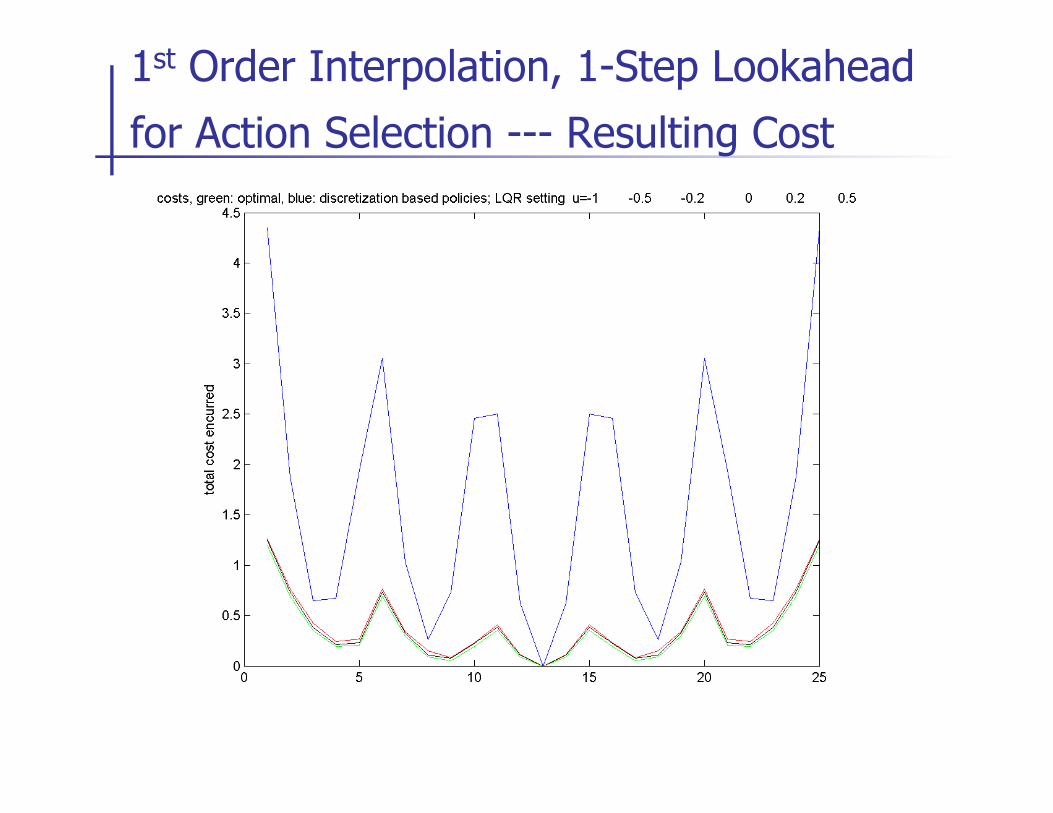
1st Order Interpolation, 1-Step Lookahead

for Action Selection --- Resulting Cost

n  Typical guarantees:

n  Assume: smoothness of cost function, transition model

n  For h à 0, the discretized value function will approach the true value function

n  To obtain guarantee about resulting policy, combine above with a general result about MDP’s:

n  One-step lookahead policy based on value function V which is close to V* is a policy that attains value close to V*

Discretization Quality Guarantees

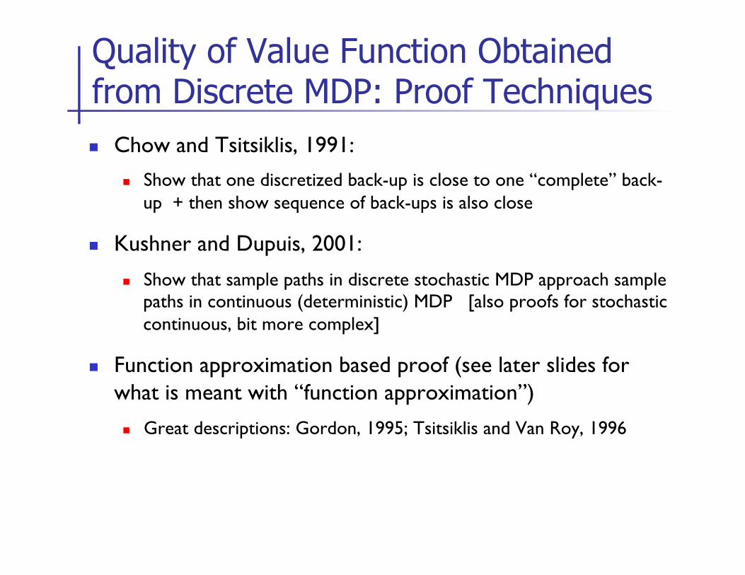
n  Chow and Tsitsiklis, 1991: n  Show that one discretized back-up is close to one “complete” back-

up + then show sequence of back-ups is also close

n  Kushner and Dupuis, 2001:

n  Show that sample paths in discrete stochastic MDP approach sample paths in continuous (deterministic) MDP [also proofs for stochastic continuous, bit more complex]

n  Function approximation based proof (see later slides for what is meant with “function approximation”)

n  Great descriptions: Gordon, 1995; Tsitsiklis and Van Roy, 1996

Quality of Value Function Obtained from Discrete MDP: Proof Techniques

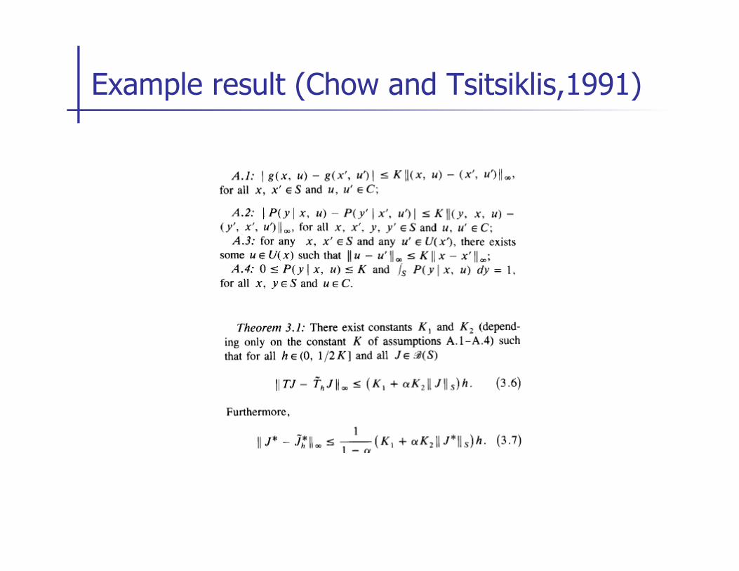
Example result (Chow and Tsitsiklis,1991)

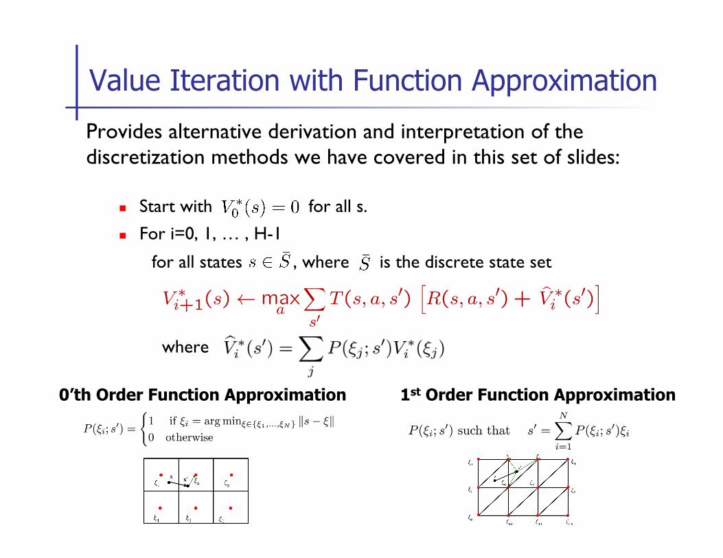
Value Iteration with Function Approximation

Provides alternative derivation and interpretation of the discretization methods we have covered in this set of slides:

n  Start with for all s. n  For i=0, 1, … , H-1

for all states , where is the discrete state set

where

0’th Order Function Approximation 1st Order Function Approximation

n  0’th order function approximation

builds piecewise constant approximation of value function

n  1st order function approximatin

builds piecewise (over “triangles”) linear approximation of value function

Discretization as function approximation

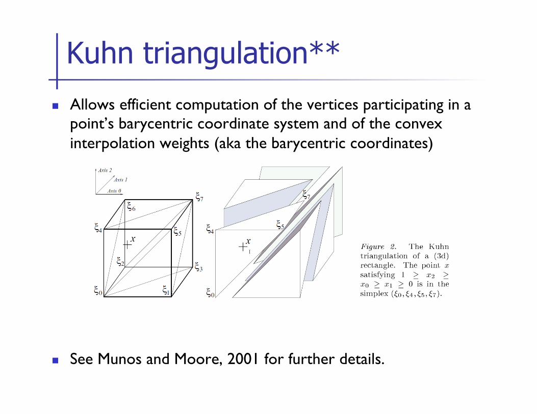
n  Allows efficient computation of the vertices participating in a point’s barycentric coordinate system and of the convex interpolation weights (aka the barycentric coordinates)

n  See Munos and Moore, 2001 for further details.

Kuhn triangulation**

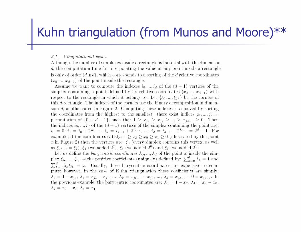
Kuhn triangulation (from Munos and Moore)**

n  One might want to discretize time in a variable way such that one discrete time transition roughly corresponds to a transition into neighboring grid points/regions

n  Discounting:

±t depends on the state and action

See, e.g., Munos and Moore, 2001 for details.

Note: Numerical methods research refers to this connection between time and space as the CFL (Courant Friedrichs Levy) condition. Googling for this term will give you more background info.

!! 1 nearest neighbor tends to be especially sensitive to having the correct match [Indeed, with a mismatch between time and space 1 nearest neighbor might end up mapping many states to only transition to themselves no matter which action is taken.]

Continuous time**

Nearest neighbor quickly degrades when time and space scale are mismatched**

h = 0.02 h = 0.1

dt= 0.1

dt= 0.01