Embed Size (px)
Citation preview
Additional Lecture Notes for the course SC4090
Discrete-time systems analysis
Ton van den Boom
October 2, 2006

2

Contents
1 Introduction 51.1 Discrete-time versus continuous-time . . . . . . . . . . . . . . . . . . . . . 51.2 Sampling and Interpolation . . . . . . . . . . . . . . . . . . . . . . . . . . 71.3 Discrete-time systems . . . . . . . . . . . . . . . . . . . . . . . . . . . . . . 12
1.3.1 Difference Equations . . . . . . . . . . . . . . . . . . . . . . . . . . 121.3.2 Discrete-time state-space models . . . . . . . . . . . . . . . . . . . 131.3.3 Linear discrete-time models . . . . . . . . . . . . . . . . . . . . . . 14
2 Operational methods for discrete-time linear systems 172.1 Discrete-time linear system operators . . . . . . . . . . . . . . . . . . . . . 172.2 Transformation of discrete-time systems . . . . . . . . . . . . . . . . . . . 21
3 System Properties and Solution techniques 233.1 Singularity input functions . . . . . . . . . . . . . . . . . . . . . . . . . . . 233.2 Classical solution of linear difference equations . . . . . . . . . . . . . . . . 24
3.2.1 Homogeneous solution of the difference equation . . . . . . . . . . . 253.2.2 Particular solution of the difference equation . . . . . . . . . . . . . 25
3.3 Discrete-time Convolution . . . . . . . . . . . . . . . . . . . . . . . . . . . 27
4 Solution of discrete-time linear state equations 314.1 State variable responses of discrete-time linear systems . . . . . . . . . . . 31
4.1.1 Homogeneous State responses . . . . . . . . . . . . . . . . . . . . . 314.1.2 The forced response of discrete-time linear systems . . . . . . . . . 334.1.3 The system output response of discrete-time linear systems . . . . . 344.1.4 The discrete-time transition matrix . . . . . . . . . . . . . . . . . . 344.1.5 System Eigenvalues and Eigenvectors . . . . . . . . . . . . . . . . . 354.1.6 Stability of discrete-time linear systems . . . . . . . . . . . . . . . . 364.1.7 Transformation of state variables . . . . . . . . . . . . . . . . . . . 37
4.2 The response of linear DT systems to the impulse response . . . . . . . . . 38
5 The Discrete-time transfer function 415.1 Introduction . . . . . . . . . . . . . . . . . . . . . . . . . . . . . . . . . . . 415.2 single-input single-output systems . . . . . . . . . . . . . . . . . . . . . . . 41
3

4 CONTENTS
5.3 relationship to the transfer function . . . . . . . . . . . . . . . . . . . . . . 425.4 System poles and zeros . . . . . . . . . . . . . . . . . . . . . . . . . . . . . 43
5.4.1 System poles and the homogeneous response . . . . . . . . . . . . . 445.4.2 System stability . . . . . . . . . . . . . . . . . . . . . . . . . . . . . 455.4.3 State space formulated systems . . . . . . . . . . . . . . . . . . . . 47

Chapter 1
Introduction
1.1 Discrete-time versus continuous-time
Engineers and Physical scientists have for many years utilized the concept of a system tofacilitate the study of the interaction between forces and matter. A system is a math-ematical abstraction that is devised to serve as a model for a dynamic phenomenon. Itrepresents the dynamic phenomenon in terms of mathematical relations among three setsof variables known as the input, the output, and the state.
The input represents, in the form of a set of time functions or sequences, the external forcesthat are acting upon the dynamic phenomenon. In similar form, the output represents themeasures of the directly observable behavior of the phenomenon. Input and output bear acause-effect relation to each other; however, depending on the nature of the phenomenon,this relation may be strong or weak.
A basic characteristic of any dynamic phenomenon is that the behavior at any time istraceable not only to the presently applied forces but also to those applied in the past. Wemay say that a dynamic phenomenon possesses a ”memory” in which the effect of pastapplied forces is stored. In formulating a system model, the state of the system represents,as a vector function of time, the instantaneous content of the ”cells” of this memory.Knowledge of the state at any time t, plus knowledge of the forces subsequently applied issufficient to determine the output (and state) at any time t ≥ t0.
As an example, a set of moving particles can be represented by a system in which thestate describes the instantaneous position and momentum of each particle. Knowledgeof position and momentum, together with knowledge of the external forces acting on theparticles (i.e., the system input) is sufficient to determine the position and momentum atany future time.
A system is, of course, not limited to modeling only physical dynamic phenomena; theconcept is equally applicable to abstract dynamic phenomena such as those encounteredin economics or other social sciences.
If the time space is continuous, the system is known as a continuous-time system. However,if the input and state vectors are defined only for discrete instants of time k, where k ranges
5

6 CHAPTER 1. INTRODUCTION
over the integers, the time space is discrete and the system is referred to as a discrete-timesystem. We shall denote a continuous-time function at time t by f(t). Similarly, a discrete-time function at time k shall be denoted by f(k). We shall make no distinction betweenscalar and vector functions. This will usually become clear from the context. Where noambiguity can arise, a function may be represented simply by f .
Figure 1.1: Illustration of discrete-time functions and quantized functions. (a) discrete-time function, (b) quantized function, (c) quantized, discrete-time function
It is important to distinguish between functions whose argument is discrete (i.e., functionsof a discrete variable) and those that in themselves vary over a discrete set. Functions ofthe latter type will be referred to as quantized functions and the systems in which theyappear will be called quantized-data systems. Thus the function illustrated in Fig. 1.1.ais a discrete-time function and the one shown in Fig.1.1.b is a quantized function. Notethat in Fig. 1.1 f(k) can range only over discrete values (which need not necessarily beuniformly spaced). A discrete-time function may, of course, be quantized as well; this isshown in Fig. 1.1.c.In certain continuous-time systems, some state variables are allowed to change only atdiscrete instants of time tk, where k ranges over the integers and where the spacing betweensuccessive instants may be arbitrary or uniform. Such systems are in effect a kind of hybridbetween a continuous- time and a discrete-time system. They are encountered whenever
1.2. SAMPLING AND INTERPOLATION 7
a continuous-time function is sampled at discrete instants of time. Although they arefrequently analyzed most easily by treating them as discrete-time systems, they differ fromdiscrete-time systems in that special consideration may have to be given to the instants oftime at which the sampling occurs. They have been given a special name and are knownas sampled-data systems.We shall be concerned here primarily with the analysis of discrete-time systems. Ourinterest in these systems is motivated by a desire to predict the performance of the physicaldevices for which this kind of system is an appropriate model. This is, however, not the onlymotive for studying discrete-time systems. A second, nearly as important reason is thatthere are many continuous-time systems that are more easily analyzed when a discrete-timemodel is fitted to them. A common example of this is the simulation of a continuous-timesystem by a digital computer. Further, a considerable body of mathematical theory hasbeen developed for the analysis of discrete-time systems. Much of this is valuable forgaining insight into the theory of continuous-time systems as well as discrete-time systems.We note that a continuous-time function can always be viewed as the limit of a timesequence whose spacing between successive terms is approaching zero.
1.2 Sampling and Interpolation
Many physical signals, such as electrical voltages produced by a sound or image recordinginstrument or a measuring device, are essentially continuous-time signals. Computers andrelated devices operate on a discrete-time axis. Continuous-time signals that are to beprocessed by such devices therefore first need be converted to discrete-time signals. Oneway of doing this is sampling.
Definition 1 Sampling.Let Tcon = IR be the continuous-time axis, and let Tdis = ZZ be the discrete-time axis.Let x(t) be a continuous-time signal with t ∈ Tcon. Then, sampling the continuous-timesignal x(t), t ∈ Tcon on the discrete-time axis Tdis with sampling period T , results in thediscrete-time signal x∗(k) defined by
x∗(k) = x(k T ) for all k ∈ Tdis (1.1)
A device that performs the sampling operation is called a sampler.
Example 2 (Sampled real harmonic) Let the continuous-time signal x, given by
x(t) = 1/2[1 − cos(2πt)], t ∈ IR
be sampled on the uniformly spaced discrete-time axis ZZ. This results in the sampled signalx∗ given by
x∗(k) = 1/2[1 − cos(2πkT )], k ∈ ZZ
8 CHAPTER 1. INTRODUCTION
original signal x sampled signal x∗
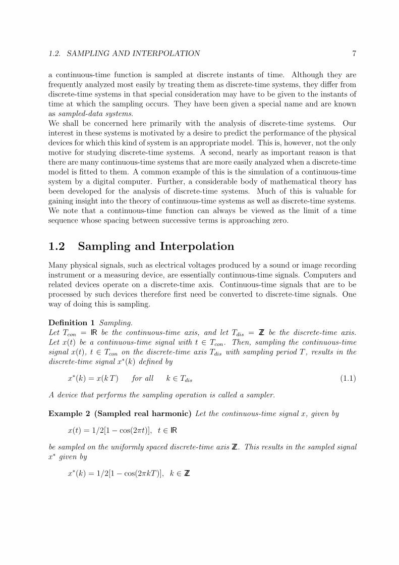
Figure 1.2: Sampling. Left: a continuous-time signal. Right: its sampled version.
The converse problem of sampling presents itself when a discrete-time device, such as acomputer, produces signals that need drive a physical instrument requiring a continuous-time signal as input. Suppose that a discrete-time signal x∗ is defined on the discrete-timeaxis Tdis and that we wish to construct from x∗ a continuous-time signal x defined onthe continuous-time axis Tcon ⊃ Tdis. There obviously are many ways to do this. Weintroduce a particular class of conversions from discrete-time to continuous-time signals,for which we reserve the term interpolation. This type of conversion has the property thatthe continuous-time signal x agrees with the discrete-time signal x∗ at the sampling times.
Definition 3 Interpolation.Let Tcon = IR be the continuous-time axis, and let Tdis = ZZ be the discrete-time axis. Letx∗(k) be a discrete-time signal with k ∈ Tdis with sampling period T . Then, any continuous-time signal x(t), t ∈ IR is called an interpolation of x∗ on Tcon, if
x(k T ) = x∗(k) for all k ∈ Tdis (1.2)
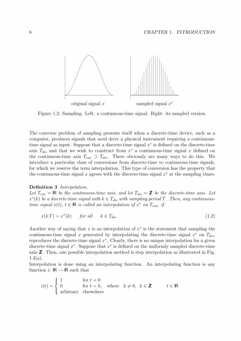
Another way of saying that x is an interpolation of x∗ is the statement that sampling thecontinuous-time signal x generated by interpolating the discrete-time signal x∗ on Tdis,reproduces the discrete-time signal x∗. Clearly, there is no unique interpolation for a givendiscrete-time signal x∗. Suppose that x∗ is defined on the uniformly sampled discrete-timeaxis ZZ. Then, one possible interpolation method is step interpolation as illustrated in Fig.1.3(a).
Interpolation is done using an interpolating function. An interpolating function is anyfunction i: IR → IR such that
i(t) =
1 for t = 00 for t = k, where k 6= 0, k ∈ ZZ
arbitrary elseweheret ∈ IR
1.2. SAMPLING AND INTERPOLATION 9
Figure 1.3: Interpolation. Top: step interpolation. Bottom: linear interpolation.
If x∗(k), k ∈ ZZ is a discrete-time signal defined on the time axis Tdis, and i an interpolatingfunction, the continuous-time signal x given by
x(t) =∑
n∈ZZ
x∗(n) i(t/T − n), t ∈ IR
is an interpolation of x∗. The reason is that by setting t = k T , with k ∈ ZZ, it follows that
x(k T ) =∑
n∈ZZ
x∗(n) i(kT/T − n) = x∗(k), k ∈ ZZ
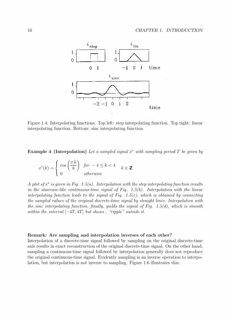
Step interpolation is achieved with the step interpolating function
istep(t) =
{
1 for 0 ≤ t < 10 otherwise
t ∈ IR
while linear interpolation is obtained with the linear interpolating function
ilin(t) =
{
1 − |t| for |t| < 10 otherwise
t ∈ IR
Another interpolation function is the sinc interpolating function
isinc(t) = sinc(π t)
Here, sinc: IR → IR is the function defined by
sinc(t) =
sin(t)
tfor t 6= 0
1 for t = 0t ∈ IR
Graphs of these interpolating functions are given in Fig. 1.4.
10 CHAPTER 1. INTRODUCTION
Figure 1.4: Interpolating functions. Top left: step interpolating function. Top right: linearinterpolating function. Bottom: sinc interpolating function.
Example 4 (Interpolation) Let a sampled signal x∗ with sampling period T be given by
x∗(k) =
cos
(
π k
8
)
for − 4 ≤ k < 4
0 otherwisek ∈ ZZ
A plot of x∗ is given in Fig. 1.5(a). Interpolation with the step interpolating function resultsin the staircase-like continuous-time signal of Fig. 1.5(b). Interpolation with the linearinterpolating function leads to the signal of Fig. 1.5(c), which is obtained by connectingthe sampled values of the original discrete-time signal by straight lines. Interpolation withthe sinc interpolating function, finally, yields the signal of Fig. 1.5(d), which is smoothwithin the interval [−4T, 4T ] but shows , “ripple” outside it.
Remark: Are sampling and interpolation inverses of each other?Interpolation of a discrete-time signal followed by sampling on the original discrete-timeaxis results in exact reconstruction of the original discrete-time signal. On the other hand,sampling a continuous-time signal followed by interpolation generally does not reproducethe original continuous-time signal. Evidently sampling is an inverse operation to interpo-lation, but interpolation is not inverse to sampling. Figure 1.6 illustrates this.

1.2. SAMPLING AND INTERPOLATION 11
Figure 1.5: Interpolation. (a) A discrete-time signal. (b) Step interpolation (c) Linearinterpolation. (d) Sinc interpolation.
Figure 1.6: Sampling and interpolation. Top: sampling is the inverse of interpolation.Bottom: interpolation is not the inverse of sampling

12 CHAPTER 1. INTRODUCTION
Remark: Analog-to-Digital and digital-to-analog conversion(a) A/D conversion. Computers and other digital equipment do not only operate on adiscrete-time axis but are also limited to finite signal ranges. Thus, apart from sam-pling, conversion of real-valued continuous-time signals to input for digital equipment alsoinvolves quantization. The combined process of sampling and quantization is called analog-to-digital (A/D) conversion.(b) D/A conversion. The inverse process of converting a quantized discrete-time signalto a real-valued continuous-time signal is called digital-to -analog (D/A) conversion. De-vices that perform D/A conversion by step interpolation are known as zero-order holdcircuits. They can function in ”real time” meaning that given the sampled signal up to,and including, time t, the continuous-time signal up to and including that same time maybe generated. Devices that perform D/A conversion by linear interpolation are known asfirst-order hold circuits. They cannot precisely function in real time because two successivesampled signal values have to be received before it is known how the continuous-time signalgoes. First-order hold circuits therefore introduce a delay, equal to the sampling period T .Sinc interpolation, finally, cannot be implemented in real time at all because all sampledsignal values need be received before any point of the continuous-time signal (except atthe sampling times) may be computed. Sinc interpolation, however, has great theoreticalimportance.
1.3 Discrete-time systems
1.3.1 Difference Equations
In continuous-time the relationships between different model variables are described withthe help of differential equations (see Rowell & Wormley [4]). In discrete-time this can bedone using difference equations. There are two different ways of describing these differenceequations. One is to directly relate inputs u to outputs y in one difference equation. Inprinciple it looks like this:
g(y(k + n), y(k + n− 1), . . . , y(k), u(k +m), u(k +m− 1), . . . , u(k)) = 0 (1.3)
where g(·, ·, . . . , ·) is an arbitrary, vector-valued, nonlinear function. The other way is towrite the difference equation as a system of first-order difference equations by introducinga number of internal variables. If we denote these internal variables by
x1(k), . . . , xn(k)
and introduce the vector notation
x(t) =
x1(k)...
xn(k)
(1.4)

1.3. DISCRETE-TIME SYSTEMS 13
we can, in principle, write a system of first-order difference equations as
x(k + 1) = f(x(k), u(k)) (1.5)
In (1.5), f(x, u) is a vector function with n components:
f(x, u) =
f1(x, u)...
fn(x, u)
(1.6)
The functions fi(x, u) are in turn functions of n + m variables, the components of the xand u vectors. Without vector notation, (1.5) becomes
x1(k + 1) = f1(x1(k), . . . , xn(k), u1(k), . . . , um(k))x2(k + 1) = f2(x1(k), . . . , xn(k), u1(k), . . . , um(k))
...xn(k + 1) = fn(x1(k), . . . , xn(k), u1(k), . . . , um(k))
(1.7)
The outputs of the model can then be calculated from the internal variables xi(k) and theinputs ui(k):
y(k) = h(x(k), u(k)) (1.8)
which written in longhand means
y1(k) = h1(x1(k), . . . , xn(k), u1(k), . . . , um(k))y2(k) = h2(x1(k), . . . , xn(k), u1(k), . . . , um(k))
...yp(k) = hp(x1(k), . . . , xn(k), u1(k), . . . , um(k))
(1.9)
1.3.2 Discrete-time state-space models
For a dynamic system the output depends on all earlier input values. This leads to the factthat it is not enough to know u(k) for k ≥ k0 in order to be able to calculate the outputy(k) for k ≥ k0. We need information about the system. By the state of the system attime k0 we mean an amount of information such that with this state and the knowledgeof u(k), k ≥ k0, we can calculate y(k), k ≥ k0. This definition is well in line with theeveryday meaning of the word “state.” It is also obvious from the definition of state thatthis concept will play a major role in the simulation of the model. The state is exactlythe information that has to be stored and updated at the simulation in order to be ableto calculate the output. Consider a general system of first-order difference equations (1.5)with the output given by (1.8):
x(k + 1) = f(x(k), u(k)) (1.10)
y(k) = h(x(k), u(k)) (1.11)
14 CHAPTER 1. INTRODUCTION
For this system the vector x(k0) is a state at time k0. The difference equation (1.10)-(1.11)with x(k0) = x0 has a unique solution for k ≥ k0. The solution can easily be found usingsuccessive substitution:Assume that we know x(k) at time k0 and u(k) for k ≥ k0. We can then according to(1.10) calculate x(k + 1).From this value we can use u(k + 1) to calculate x(k + 2), again using (1.10). We cancontinue and calculate x(k) for all k > k0. The output y(k), k ≥ k0, can then also becomputed according to (1.11).We have thus established that the variables x1(k), . . . , xn(k) or, in other words, the vector
x(k) =
x1(k)...
xn(k)
in the internal model description (1.10)-(1.11) is a state for the model. Herein lies theimportance of this model description for simulation. The model (1.10)-(1.11) is thereforecalled a state-space model, the vector x(k) the state vector, and its components xi(k) statevariables. The dimension of x(k), that is, n, is called the model order.State-space models will be our standard model for dynamic discrete-time systems. Inconclusion, we have the following model:Discrete-time state space models
x(k + 1) = f(x(k), u(k)) k = 0, 1, 2, . . . (1.12)
y(k) = h(x(k), u(k)) (1.13)
u(k): input at time k , an m-dimensional column vector.y(k): output at time k , a p-dimensional column vector.x(k): state at time k , an n-dimensional column vector.The model is said to be n-th order. For a given initial value x(k0) = x0, (1.12)-(1.13)always has a unique solution.
1.3.3 Linear discrete-time models
The model (1.12)-(1.13) is said to be linear if f(x, u) and h(x, u) are linear functions of xand u:
f(x, u) = Ax+Bu (1.14)
h(x, u) = Cx+Du (1.15)
Here the matrices have the following dimensions
A : n× n B : n×m
C : p× n D : p×m
1.3. DISCRETE-TIME SYSTEMS 15
If these matrices are independent of time the model (1.14)-(1.15) is said to be linear andtime invariant.The model (1.3) is said to be linear if g(·, ·, . . . , ·) is a linear function in y and u:
g(y(k+n), y(k+n−1), . . . , y(k), u(k+m), u(k+m−1), . . . , u(k))
= a0 y(k+n)+an−1 y(k+n−1)+. . .+a0 y(k)
−bm u(k+m)−bm−1 u(k+m−1)−. . .−b0 u(k) = 0
or
a0 y(k+n)+an−1 y(k+n−1)+. . .+a0 y(k) = bm u(k+m)+bm−1 u(k+m−1)+. . .+b0 u(k) (1.16)
Example 5 (Savings account)Suppose that y(k) represents the balance of a savings account at the beginning of day k ,and u(k) the amount deposited during day k. If interest is computed and added daily at arate of α · 100%, the balance at the beginning of day k + 1 is given by
y(k + 1) = (1 + α)y(k) + u(k), k = 0, 1, 2, · · · (1.17)
This describes the savings account as a discrete-time system on the time axis ZZ+. If theinterest rate α does not change with time, the system is time-invariant; otherwise, it istime-varying.
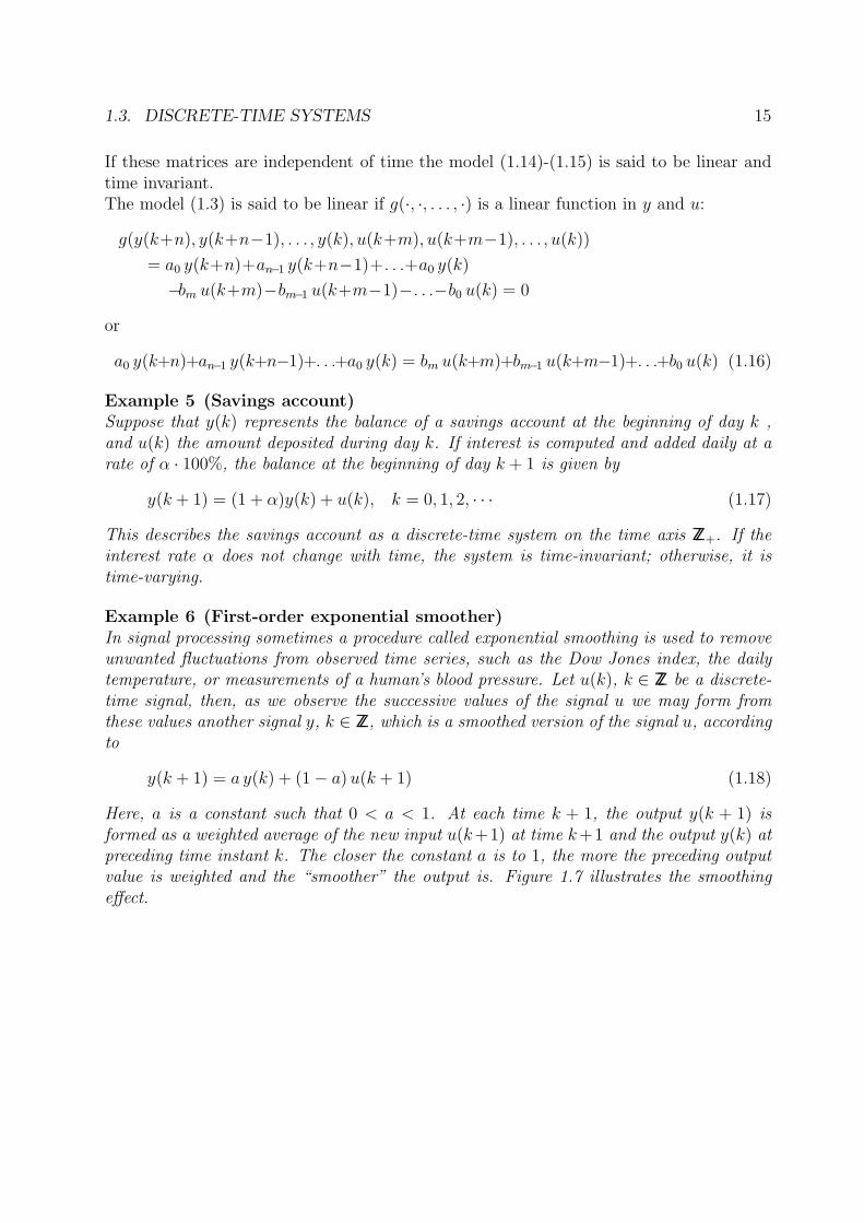
Example 6 (First-order exponential smoother)In signal processing sometimes a procedure called exponential smoothing is used to removeunwanted fluctuations from observed time series, such as the Dow Jones index, the dailytemperature, or measurements of a human’s blood pressure. Let u(k), k ∈ ZZ be a discrete-time signal, then, as we observe the successive values of the signal u we may form fromthese values another signal y, k ∈ ZZ, which is a smoothed version of the signal u, accordingto
y(k + 1) = a y(k) + (1 − a) u(k + 1) (1.18)
Here, a is a constant such that 0 < a < 1. At each time k + 1, the output y(k + 1) isformed as a weighted average of the new input u(k+1) at time k+1 and the output y(k) atpreceding time instant k. The closer the constant a is to 1, the more the preceding outputvalue is weighted and the “smoother” the output is. Figure 1.7 illustrates the smoothingeffect.
16 CHAPTER 1. INTRODUCTION
0 5 10 15 20 25 30 35 40 45 50−2
−1
0
1
2
k −−−>
u(k)
−−−
>
0 5 10 15 20 25 30 35 40 45 50−1.5
−1
−0.5
0
0.5
1
k −−−>
y(k)
−−−
>
Figure 1.7: Exponential smoothing (a = 0.8)

Chapter 2
Operational methods fordiscrete-time linear systems
In this chapter we will consider operational methods for discrete-time linear systems. Forthe continuous-time case see Rowell & Wormley [4].
2.1 Discrete-time linear system operators
Consider a discrete-time signal f(k), for k ∈ ZZ. All linear time-invariant systems may berepresented by an interconnection of the following primitive operators:
1. The constant scaling operator: The scaling operator multiplies the input functionby a constant factor. It is denoted by the value of the constant, either numericallyor symbolically, for example 2.0{}, or α{}.
2. The forward shift operator: The shift operator, designated Z{}, shifts the inputsignal in one step ahead in time:
y(k) = Z{f(k)} = f(k + 1)
3. The backward shift operator: The shift operator, designated Z−1{}, shifts the in-put signal in one step back in time:
y(k) = Z−1{f(k)} = f(k − 1)
4. The difference operator: The difference operator, written ∆{}, generates the incre-ment of the input f(k):
y(k) = ∆{f(k)} = f(k) − f(k − 1)
17
18CHAPTER 2. OPERATIONAL METHODS FOR DISCRETE-TIME LINEAR SYSTEMS
5. The summation operator: The summation operator, written ∆−1{}, generates thesummation of the input f(k):
y(k) = ∆−1{f(k)} =k∑
m=0
f(m)
where it is assumed that at time k < 0, the output y(k) = 0. If an initial conditiony(−1) is specified,
y(k) = ∆−1{f(k)} + y(−1)
and a separate summing block is included at the output of the summation block toaccount for the initial condition.
6. The identity operator: The identity operator leaves the value f(k) unchanged, thatis:
y(k) = I{f(k)} = f(k)
7. The null operator: The null operator N{} identically produces an output of zero forany input, that is,
y(k) = N{f(k)} = 0
Remark 1: Note that by substituting f(k − 1) = Z−1{f(k)} we find that
∆{} = I{} − Z−1{}
Remark 2: The discrete-time operators Z, Z−1, ∆, ∆−1, I and N are linear operators.Therefore all properties for linear operators will also hold for these discrete-time operators.
Block diagram of a discrete-time system
The block diagram of the state-space description of a linear discrete-time system is equiv-alent to the one for continuous-time systems if we substitute the backward shift block Z−1
for the integral block. (In the book of Rowell & Wormley [4] it is the block S−1 as in Fig.2.1.) We obtain the block diagram of figure 2.1.The block diagram of general second-order discrete-time state system
[
x1(k + 1)x2(k + 1)
]
=
[
a11 a12
a21 a22
] [
x1(k)x2(k)
]
+
[
b1b2
]
u(k)
y(k) =[
c1 c2]
[
x1(k)x2(k)
]
+ d u(k)
is shown in figure 2.2.

2.1. DISCRETE-TIME LINEAR SYSTEM OPERATORS 19
Figure 2.1: Vector block diagram for a linear discrete-time system described by state spacesystem dynamics
Figure 2.2: Block diagram for a state equation-based second-order discrete-time system

20CHAPTER 2. OPERATIONAL METHODS FOR DISCRETE-TIME LINEAR SYSTEMS
Input-output linear discrete-time system models
For systems that have only one input and one output, it is frequently convenient to workwith the classical system input-output description in Eq. (1.16) consisting of a single n-thorder difference equation relating the output to the system input:
an y(k + n) + an−1 y(k + n− 1) + . . .+ a0 y(k)
= bm u(k +m) + bm−1 u(k +m− 1) + . . .+ b0 u(k) (2.1)
The constant coefficients ai and bi are defined by the system parameters and for causalsystems there holds: m ≤ n.
Equation (2.1) may be written in operational form using polynomial operators as:
[
an Zn + an−1 Z
n−1 + . . .+ a0
]
{y} =[
bm Zm + bm−1 Z
m−1 + . . .+ b0]
{u} (2.2)
If the inverse operator[
an Zn + an−1 Z
n−1 + . . . + a0
]−1
exists, it may be applied to eachside to produce an explicit operational expression for the output variable:
y(k) =bm Z
m + bm−1 Zm−1 + . . .+ b0
an Zn + an−1 Zn−1 + . . .+ a0
{u(k)} (2.3)
The operational description of the system dynamics has been reduced to the form of asingle linear operator, the dynamic transfer operator H{},
y(k) = H{u(k)} (2.4)
where
H{} =bm Z
m + bm−1 Zm−1 + . . .+ b0
an Zn + an−1 Zn−1 + . . .+ a0
{} (2.5)
In (1.14)-(1.15), the state space description was given for a linear discrete-time system:
x(k + 1) = Ax(k) +Bu(k) (2.6)
y(k) = Cx(k) +Du(k) (2.7)
The matrix transfer operator for this system can be computed by:
H{} =C adj(Z I − A)B + det[Z I −A]D
det[Z I −A](2.8)

2.2. TRANSFORMATION OF DISCRETE-TIME SYSTEMS 21
2.2 Transformation of discrete-time systems
State realization of a polynomial difference system
The polynomial difference system (2.3), described by
[
bm Zm + bm−1 Z
m−1 + . . .+ b0]
y(k) =[
an Zn + an−1 Z
n−1 + . . .+ a0
]
u(k)
has a state realization
x(k + 1) = Ax(k) +Bu(k)
y(k) = Cx(k) +Du(k)
such that
A =
0 1 · · · 0 0
0 0. . . 0 0
......
. . ....
...0 0 · · · 1 00 0 · · · 0 1
−a0/an −a1/an · · · −an−2/an −an−1/an
B =
00...00
1/an
C =[
b0−a0bn/an b1−a1bn/an · · · bn−2−an−2bn/an bn−1−an−1bn/an]
D = bn/an
Polynomial realization of a state system
The state difference system (2.6)-(2.7), described by
x(k + 1) = Ax(k) +Bu(k)
y(k) = Cx(k) +Du(k)
has a polynomial realization
[
det[Z I − A]] y(k) =[
C adj(ZI − A)B + det[ZI − A]D] u(k) (2.9)
and a transfer operator
H = C (ZI −A)−1B + D (2.10)
=C adj(ZI − A)B + det[ZI − A]D
det[Z I −A](2.11)

22CHAPTER 2. OPERATIONAL METHODS FOR DISCRETE-TIME LINEAR SYSTEMS
Example 7 (Polynomial to state-space)Consider the difference system
16 y(k + 3) − 20 y(k + 2) + 8 y(k + 1) − y(k) = 5 u(k + 2) − 7 u(k + 1) + 2 u(k)
the state space realization is given by
x1(k + 1)x2(k + 1)x3(k + 1)
=
0 1 00 0 1
1/16 −8/16 20/16
x1(k + 1)x2(k + 1)x3(k + 1)
+
00
1/16
u(k)
y(k) =[
2 −7 5]
x1(k)x2(k)x3(k)
Example 8 (State-space to polynomial)Consider the state system
[
x1(k + 1)x2(k + 1)
]
=
[
−0.5 1.5−1 2
] [
x1(k)x2(k)
]
+
[
20
]
u(k)
y(k) =[
1 1]
[
x1(k)x2(k)
]
+ 2 u(k)
The determinant of [Z I −A] is
det[Z I −A] = Z2 − 1.5Z + 0.5
and the adjoint of [Z I −A] is
adj
[
Z + 0.5 −1.51 Z − 2
]
=
[
Z − 2 1.5−1 Z + 0.5
]
Further we compute
C adj(ZI −A)B + det[ZI −A]D =
=[
1 1]
[
Z − 2 1.5−1 Z + 0.5
][
20
]
+ (Z2 − 1.5Z + 0.5) 2
= (2Z − 6) + (2Z2 − 3Z + 1)
= 2Z2 − Z − 5
So the related difference equation is given by equation (2.9):
(Z2 − 1.5Z + 0.5) y(k) = (2Z2 − Z − 5) u(k)
or
y(k + 2) − 1.5 y(k + 1) + 0.5 y(k) = 2 u(k + 2) − u(k + 1) − 5 u(k)

Chapter 3
System Properties and Solutiontechniques
In this chapter we discuss system properties and solution techniques for discrete-timesystems. (For the continuous case, see Rowell & Wormley [4], chapter 8).
3.1 Singularity input functions
In Rowell & Wormley [4], chapter 8, some singularity input functions for continuous-timesystems were defined. In this section we redefine some of the functions for discrete-time:
The Unit Step Function: The discrete-time unit step function us(k), k ∈ ZZ is definedas:
us(k) =
{
0 for k < 01 for k ≥ 0
(3.1)
The Unit Impulse Function: The discrete-time unit Impulse function δ(k), k ∈ ZZ isdefined as:
δ(k) =
{
1 for k = 00 for k 6= 0
(3.2)
Note that for discrete-time the definition of a function δT (k) is not appropriate.The discrete-time impulse function (or discrete-time Dirac delta function) has theproperty that
∞∑
m=−∞
δ(m) = 1
23

24 CHAPTER 3. SYSTEM PROPERTIES AND SOLUTION TECHNIQUES
The unit ramp function: The discrete-time unit ramp function ur(k), k ∈ ZZ is definedto be a linearly increasing function of time with a unity increment:
ur(k) =
{
0 for k ≤ 0k for k > 0
(3.3)
Note that
∆{ur(k + 1)} = ur(k + 1) − ur(k) = us(k) (3.4)
and
∆{us(k)} = us(k) − us(k − 1) = δ(k) (3.5)
and also in the reverse direction:
∆−1{δ(k)} =k∑
m=0
δ(k) = us(k) (3.6)
and
∆−1{us(k)} =k∑
m=0
us(k) = ur(k + 1) (3.7)
3.2 Classical solution of linear difference equations
In this section we briefly review the classical method for solving a linear nth-order ordinarydifference equation with constant coefficients, given by
y(k + n) + an−1 y(k + n− 1) + . . .+ a0 y(k)
= bm u(k +m) + bm−1 u(k +m− 1) + . . .+ b0 u(k) (3.8)
where in general m ≤ n. We define the forcing function
f(k) = bm u(k +m) + bm−1 u(k +m− 1) + . . .+ b0 u(k) (3.9)
which is known, because u(k) is known for all k ∈ ZZ. Eq. (3.8) now becomes
y(k + n) + an−1 y(k + n− 1) + . . .+ a0 y(k) = f(k) (3.10)
The task is to find a unique function y(k) for k ≥ k0 that satisfies the difference equation(3.8) given the forcing function f(k) and a set of initial conditions y(k0), y(k0+1), . . . , y(k0+n− 1).The general solution to Eq. (3.8) may be derived as the sum of two solution components
y(k) = yh(k) + yp(k) (3.11)
where yh is the solution of the homogeneous equation (so for f(k) = 0) and yp(k) is a par-ticular solution that satisfies (3.10) for the specific f(k) (but arbitrary initial conditions).
3.2. CLASSICAL SOLUTION OF LINEAR DIFFERENCE EQUATIONS 25
3.2.1 Homogeneous solution of the difference equation
The homogeneous difference equation (an 6= 0) is given by
an y(k + n) + an−1 y(k + n− 1) + . . .+ a0 y(k) = 0 (3.12)
The standard method of solving difference equations assumes there exists a solution of theform y(k) = C λk, where λ and C are both constants. Substitution in the homogeneousequation gives:
C(
anλn + an−1λ
n−1 + . . .+ a0
)
λk = 0 (3.13)
For any nontrivial solution, C is nonzero and λk is never zero, we require that
anλn + an−1λ
n−1 + . . .+ a0 = 0 (3.14)
For an nth-order system with an 6= 0, there are n (complex) roots of the characteristicpolynomial and n possible solution terms Ci λ
ki (i = 1, . . . , n), each with its associated
constant. The homogeneous solution will be the sum of all such terms:
yh(k) = C1 λk1 + C2 λ
k2 + . . .+ Cn λ
kn (3.15)
=n∑
i=1
Ci λki (3.16)
The n coefficients Ci are arbitrary constants and must be found from the n initial condi-tions.
If the characteristic polynomial has repeated roots, that is λi = λj for i 6= j, there are notn linearly independent terms in the general homogeneous response (3.16). In general if aroot λ of multiplicity m occurs, the m components in the general solution are
C1 λk , C2 k λ
k , . . . , Cm km−1 λm
If one or more roots are equal to zero (λi = 0), the solution C λk = 0 has no meaning.In that case we add a term C δ(k − k0) to the general solution. If the root λ = 0 hasmultiplicity m, the m components in the general solution are
C1 δ(k − k0) , C2 δ(k − k0 − 1) , . . . , Cm δ(k − k0 −m+ 1)
3.2.2 Particular solution of the difference equation
Also for discrete-time systems, the method of undetermined coefficients can be used (see[4], page 255-257), where we use table 3.1 to find the particular solutions for some specificforcing functions.

26 CHAPTER 3. SYSTEM PROPERTIES AND SOLUTION TECHNIQUES
Terms in u(k) Assumed form for yp(k) Test value
α β1 0
α kn , (n = 1, 2, 3, . . .) βn kn + βn−1 k
n−1 + . . .+ β1 k + β0 0
α λk β λk λ
α cos(ωk) β1 cos(ωk) + β2 sin(ωk) jω
α sin(ωk) β1 cos(ωk) + β2 sin(ωk) jω
Figure 3.1: Definition of Particular yp(k) using the method of undetermined coefficients
Example 9 (Solution of a difference equation)Consider the system described by the difference equation
2 y(k + 3) + y(k + 2) = 7 u(k + 1) − u(k)
Find the system response to a ramp input u(k) = k and initial conditions given by y(0) = 2,y(1) = −1 and y(2) = 2.
Solution:homogeneous solution: The characteristic equation is:
2 λ3 + λ2 = 0
which has a root λ1 = −0.5 and a double root λ2,3 = 0. The general solution of thehomogeneous equation is therefore
yh(k) = C1 (−0.5)k + C2 δ(k) + C3 δ(k − 1)
particular solution: From table 3.1 we find that for u(k) = k, the particular solution isselected:
yp = β1 k + β0
Testing gives:
2 (β1 (k + 3) + β0) + (β1 (k + 2) + β0) = 7 (k + 1) − k = 6 k + 7
We find β1 = 2 and β0 = −3 and so the particular solution is
yp(k) = 2 k − 3
complete solution: The complete solution will have the form:
y(k) = yh(k) + yp(k) = C1 (−0.5)k + C2 δ(k) + C3 δ(k − 1) + 2 k − 3
3.3. DISCRETE-TIME CONVOLUTION 27
Now the initial conditions are evaluated in k = 0, k = 1 and k = 2.
y(0) = C1 (−0.5)0 + C2 δ(0) + C3 δ(0 − 1) + 2 0 − 3
= C1 + C2 − 3 = 2
y(1) = C1 (−0.5)1 + C2 δ(1) + C3 δ(1 − 1) + 2 1 − 3
= −C1 0.5 + C3 − 1 = −1
y(2) = C1 (−0.5)2 + C2 δ(2) + C3 δ(2 − 1) + 2 2 − 3
= C1 0.25 + 1 = 2
We find a solution for C1 = 4, C2 = 1, C3 = 2 and so the final solution becomes:
y(k) = 4 (−0.5)k + δ(k) + 2 δ(k − 1) + 2 k − 3
3.3 Discrete-time Convolution
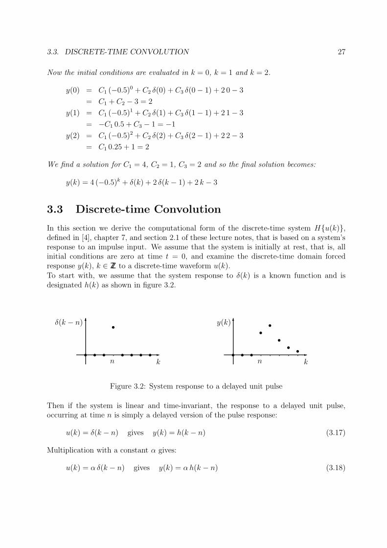
In this section we derive the computational form of the discrete-time system H{u(k)},defined in [4], chapter 7, and section 2.1 of these lecture notes, that is based on a system’sresponse to an impulse input. We assume that the system is initially at rest, that is, allinitial conditions are zero at time t = 0, and examine the discrete-time domain forcedresponse y(k), k ∈ ZZ to a discrete-time waveform u(k).To start with, we assume that the system response to δ(k) is a known function and isdesignated h(k) as shown in figure 3.2.
-
6
s s s
s
s s s s
δ(k − n)
n k-
6
s s s
s
s
s
s
s
y(k)
n k
Figure 3.2: System response to a delayed unit pulse
Then if the system is linear and time-invariant, the response to a delayed unit pulse,occurring at time n is simply a delayed version of the pulse response:
u(k) = δ(k − n) gives y(k) = h(k − n) (3.17)
Multiplication with a constant α gives:
u(k) = α δ(k − n) gives y(k) = αh(k − n) (3.18)

28 CHAPTER 3. SYSTEM PROPERTIES AND SOLUTION TECHNIQUES
The input signal u(k) may be considered to be the sum of non-overlapping delayed pulsespn(k):
u(k) =∞∑
n=−∞
pn(k) (3.19)
where
pn(k) =
{
u(k) for k = n0 for k 6= n
(3.20)
Each component pn(k) may be written in terms of a delayed unit pulse δ(k), that is
pn(k) = u(n)δ(k − n)
From equation (3.18) it follows that for a delayed version of the pulse response, multipliedby a constant u(n) we obtain the output y(k) = u(n) h(k − n).For an input
u(k) =∞∑
n=−∞
pn(k)
we can use the principle of superposition and the output can be written as a sum of allresponses to pn(k), so:
y(k) =∞∑
n=−∞
u(n) h(k − n) (3.21)
This sum is denoted as the convolution sum for discrete-time systems.For physical systems, the pulse response h(k) is zero for time k < 0, and future componentsof the input do not contribute to the sum. So the convolution sum becomes:
y(k) =k∑
n=−∞
u(n) h(k − n) (3.22)
The convolution operation is often denoted by the symbol ∗ :
y(k) = u(k) ∗ h(k) =k∑
n=−∞
u(n) h(k − n) (3.23)
Example 10 (Discrete-time convolution)The first-order exponential smoother of example 6 is described by the difference equation
y(k + 1) = a y(k) + (1 − a) u(k + 1)
By repeated substitution it easily follows that if y(k) = 0 for k < n0, the output of thesystem is given by
y(k) = (1 − a)k∑
n=n0
ak−n u(n) k ≥ n0

3.3. DISCRETE-TIME CONVOLUTION 29
assuming that the input u(k) is such that the sum converges, and let n0 approach to −∞.Then the response of the system takes the form
y(k) = (1 − a)k∑
n=−∞
ak−n u(n) k ∈ ZZ
Define the function h such that
h(k) =
{
0 for k < 0(1 − a)ak for k ≥ 0
= (1 − a)ak us(k)
we see that on the infinite time axis the system may be represented as the convolution sum
y(k) =∞∑
n=−∞
h(k − n) u(k)

30 CHAPTER 3. SYSTEM PROPERTIES AND SOLUTION TECHNIQUES

Chapter 4
Solution of discrete-time linear stateequations
In this chapter we will discuss the general solution of discrete-time linear state equations.(For the continuous-time case, see Rowell & Wormley [4], chapter 10).
4.1 State variable responses of discrete-time linear
systems
In this chapter we examine the responses of linear time-invariant discrete-time models inthe standard state equation form
x(k + 1) = Ax(k) +Bu(k) (4.1)
y(k) = Cx(k) +Du(k) (4.2)
The solution proceeds in two steps: First the state-variable response x(k) is determinedby solving the set of first-order state equations Eq. (4.1), and then the state response issubstituted into the algebraic output equations, Eq. (4.2) in order to compute y(k).
4.1.1 Homogeneous State responses
The state variable response of a system described by Eq. (4.1) with zero input and anarbitrary set of initial conditions x(0) is the solution of the set of n homogeneous first-order difference equations
x(k + 1) = Ax(k) (4.3)
We can find the solution by successive substitution. Note that x(1) = Ax(0) and x(2) =Ax(1), so by substitution we obtain x(2) = A2 x(0). Proceeding in this way we derive:
x(k) = Ak x(0) (4.4)
31

32 CHAPTER 4. SOLUTION OF DISCRETE-TIME LINEAR STATE EQUATIONS
The solution is often written as:
x(k) = Φ(k) x(0) (4.5)
where Φ(k) = Ak is defined to be the state transition matrix.
Example 11 (First-order exponential smoother)In example 6, the first-order exponential smoother was presented. The state differencerepresentation and output equations are
x(k + 1) = a x(k) + a(1 − a) u(k)
y(k) = x(k) + (1 − a) u(k), k ∈ ZZ
The homogeneous state difference equation is given by
x(k + 1) = ax(k)
It follows that the 1 × 1 state transition matrix is given by
Φ(k) = AA · · ·A = a · a · · · a = ak, k > 0, k ∈ ZZ.
Example 12 (Second-order exponential smoother)Consider now the second-order smoother described by the difference equation
y(k + 2) − a1y(k + 1) − a0y(k) = b2u(k + 2) + b1u(k + 1), k ∈ ZZ
Since the order of the system is N = 2, the dimension of the state is also 2. According tothe transformation formulae in section 2.2, the system may be represented in state form as
x(k + 1) =
[
a1 1a0 0
]
x(k) +
[
b1 + a1b2a0b2
]
u(k),
y(k) =[
1 0]
+ b2u(k), k ∈ ZZ
The homogeneous state difference equation is
x(k + 1) =
[
a1 1a0 0
]
x(k) = Ax(k) (4.6)
Then the 2 × 2 state transition matrix is given by
Φ(k) = A · A · · · A = Ak
For instance, let us take numerical values a0 = 0, and a1 = 1
2, then
A =
[
1
21
0 0
]
; (4.7)
4.1. STATE VARIABLE RESPONSES OF DISCRETE-TIME LINEAR SYSTEMS 33
and it can be seen that
Φ(k) =
[
(1
2)k 2(1
2)k
0 0
]
; k ≥ 0, k ∈ ZZ (4.8)
Consider homogeneous system (4.6) with system matrix (4.7) and initial condition
x(0) =
[
164
]
Then for k = 3 we find:
x(3) = Φ(3) x(0) = Φ(k) =
[
(1
2)3 2(1
2)3
0 0
] [
164
]
=
[
1/8 1/40 0
][
164
]
=
[
30
]
(4.9)
4.1.2 The forced response of discrete-time linear systems
The solution of the inhomogeneous discrete-time state equation
x(k + 1) = Ax(k) +Bu(k) (4.10)
(4.11)
follows easily by induction
x(k + 2) = Ax(k + 1) +Bu(k + 1)
= A(
Ax(k) +Bu(k))
+Bu(k + 1)
= A2x(k) + ABu(k) +Bu(k + 1)
Proceeding in this way we derive
x(k) = Ak x(0) +k−1∑
m=0
Ak−m−1B u(m) (4.12)
for k ≥ 1. For k ≤ 0, the summation does not contribute to the solution, and we thereforemultiply this term by us(k − 1), which is zero for k ≤ 0. We obtain:
x(k) = Ak x(0) +k−1∑
m=0
Ak−m−1B u(m) us(k − 1) (4.13)
Example 13 (Second-order exponential smoother)Consider again the second order exponential smoother of example 12. Since
A(k) =
[
a1 1a0 0
]
; B(k) =
[
b1 + a1b2a0b2
]
yields
x(k) = Ak x(0) +k−1∑
m=0
Ak−m−1B u(m) us(k − 1)

34 CHAPTER 4. SOLUTION OF DISCRETE-TIME LINEAR STATE EQUATIONS
Let us adopt the numerical values a0 = 0, a1 = 1
2, b1 = 1 and b2 = 0 resulting in A as in
(4.7) and B, C, and D as follows
B =
[
10
]
; C =[
1 0]
; D = 0 (4.14)
With (4.8) we may express the forced response of this system as
x(k) =
[
(1
2)k 2(1
2)k
0 0
]
x(0) +k−1∑
m=0
[
(1
2)k−m−1
0
]
u(m) us(k − 1)
4.1.3 The system output response of discrete-time linear systems
The output response of a discrete-time linear system is easily derived by substitution of(4.13) in (4.2):
y(k) = Cx(k) +Du(k)
= C
(
Ak x(0) +k−1∑
m=0
Ak−m−1B u(m) us(k − 1)
)
+Du(k)
= CAk x(0) +k−1∑
m=0
CAk−m−1B u(m) us(k − 1) +Du(k)
So the forced output response is given by
y(k) = CAk x(0) +k−1∑
m=0
CAk−m−1B u(m) us(k − 1) +Du(k)
Example 14 (Second-order exponential smoother)Based on example 13, we may obtain for the second-order exponential smoother the follow-ing output response
y(k) = (1
2)kx1(0) +
k−1∑
m=0
(1
2)k−m−1 u(m) us(k − 1)
= (1
2)kx1(0) +
k−1∑
m=0
(1
2)m u(k −m− 1) us(k − 1)
4.1.4 The discrete-time transition matrix
The discrete-time transition matrix Φ(k) has the following properties:
1. Φ(0) = I.
2. Φ(−k) = Φ−1(k).
4.1. STATE VARIABLE RESPONSES OF DISCRETE-TIME LINEAR SYSTEMS 35
3. Φ(k1)Φ(k2) = Φ(k1 + k2), and so
x(k2) = Φ(k2)x(0) = Φ(k2)Φ(−k1)x(k1) = Φ(k2 − k1)x(k1)
or
x(k2) = Φ(k2 − k1)x(k1)
4. If A is a diagonal matrix, then Ak is also a diagonal matrix and each element is thek-th power of the corresponding diagonal element of the A matrix, that is, akii.
4.1.5 System Eigenvalues and Eigenvectors
Let A be the system matrix of system (4.1)-(4.2). The values λi satisfying the equation
λimi = Ami for mi 6= 0 (4.15)
are known as the eigenvalues, or characteristic values, of A. The corresponding columnvectors m are defined as eigenvectors, or characteristic vectors. Equation (4.15) can berewritten as:
(λiI − A)mi = 0 (4.16)
The condition for a non-trivial solution of such a set of linear equations is that
det(λiI − A) = 0 (4.17)
which is defined as the characteristic polynomial of the A matrix. Eq. (4.17) may bewritten as
λn + an−1λn−1 + . . .+ a1λ+ a0 = 0 (4.18)
or, in factored form in terms of its roots λ1, . . . , λn,
(λ− λ1)(λ− λ2) · · · (λ− λn) = 0 (4.19)
Define
M =[
m1 m2 · · · mn
]
and
Λ =
λ1 0 · · · 0
0 λ2
......
. . .
0 · · · λn
36 CHAPTER 4. SOLUTION OF DISCRETE-TIME LINEAR STATE EQUATIONS
then
Λk =
λk1 0 · · · 0
0 λk2...
.... . .
0 · · · λkn
and
Φ(k) = Ak = (M ΛM−1)k = M ΛkM−1
4.1.6 Stability of discrete-time linear systems
For asymptotic stability, the homogeneous response of the state vector x(k) returns to theorigin for arbitrary initial conditions x(0) at time k → ∞, or
limk→∞
x(k) = limk→∞
Φ(k) x(0) = limk→∞
M ΛkM−1 x(0) = 0
for any x(0). All the elements are a linear combination of the modal components λki ,therefore, the stability of a system response depends on all components decaying to zerowith time. If |λ| > 1, the component will grow exponentially with time and the sum isby definition unstable. The requirements for system stability may therefore be summarized:
A linear discrete-time system described by the state equation x(k + 1) = Ax(k) + b u(k) isasymptotically stable if and only if all eigenvalues have magnitude smaller than one.
Three other separate conditions should be considered:
1. If one or more eigenvalues, or pair of conjugate eigenvalues, has a magnitude largerthan one, there is at least one corresponding modal component that increases expo-nentially without bound from any initial condition, violating the definition of stabil-ity.
2. Any pair of conjugate eigenvalues that have magnitude equal to one, λi,i+1 = e±jω,generates an undamped oscillatory component in the state response. The magni-tude of the homogeneous system response neither decays nor grows but continues tooscillate for all time at a frequency ω. Such a system is defined to be marginallystable.
3. An eigenvalue λ = 1 generates a model exponent λk = 1k = 1 that is a constant.The system response neither decays or grows, and again the system is defined to bemarginally stable.

4.1. STATE VARIABLE RESPONSES OF DISCRETE-TIME LINEAR SYSTEMS 37
Example 15 (Second-order exponential smoother)Consider the second-order exponential smoother of example 12. With the numerical valuesa0 = 0, a1 = 1
2, b1 = 1 and b2 = 0, the system matrices are given by 4.7 and 4.14. The
characteristic polynomial of the matrix A is
det(λI −A) = det
[
λ− 1
2−1
0 λ
]
= λ(λ−1
2) (4.20)
As a result, the eigenvalues of A are λ1 = 0 and λ2 = 1
2. Thus since all its eigenvalues are
less than one, this discrete-time system is stable.
4.1.7 Transformation of state variables
Consider the discrete-time system
x(k + 1) = Ax(k) +Bu(k) (4.21)
y(k) = Cx(k) +Du(k) (4.22)
and let consider the eigenvalue decomposition of the A matrix
A = M ΛM−1
Then this system can be transformed to the diagonal form
x′(k + 1) = A′x′(k) +B′u(k) (4.23)
y(k) = C ′x′(k) +D′u(k) (4.24)
by choosing
x′(k) = M−1x(k)
A′ = M−1AM = Λ
B′ = M−1B
C ′ = CM
D′ = D
Example 16 (Second-order exponential smoother)Consider the second-order exponential smoother of example 12 and example 15. It can befound that the corresponding eigenvectors are
v1 =
[
1−1
2
]
; v2 =
[
10
]
; (4.25)
It follows that the modal transformation matrix V , its inverse V −1 and the diagonal matrixΛ are
V =
[
1 1−1
20
]
; V −1 =
[
0 −21 2
]
; Λ =
[
0 00 1
2
]
; (4.26)

38 CHAPTER 4. SOLUTION OF DISCRETE-TIME LINEAR STATE EQUATIONS
Thus, after modal transformation the system is represented as in Eqs. (4.23) and (4.24)where
A′ = V −1AV = Λ =
[
0 00 1
2
]
;
B′ = V −1B =
[
01
]
; C ′ = CV =[
1 1]
;
4.2 The response of linear DT systems to the impulse
response
Let
u(k) = δ(k)
where δ(k) is the impulse response, defined in Eq. (3.2).Following Eq. (4.15) we find
y(k) = CAk x(0) +k−1∑
m=0
CAk−m−1B δ(m) us(k − 1) +Dδ(k) (4.27)
Note that the termk−1∑
m=0
CAk−m−1B δ(m) us(k − 1)
only gives a contribution for m = 0, so:
k−1∑
m=0
CAk−m−1B δ(m) us(k − 1) = CAk−1B us(k − 1)
Eq. (4.27) now becomes
y(k) = CAk x(0) + CAk−1B us(k − 1) +Dδ(k) (4.28)
which is the impulse response of a linear DT system.
Remark:Note that a state transformation does not influence the input-output behaviour of thesystem. We therefore may use the diagonal form of the state space description of thesystem. The impulse response becomes:
y(k) = C ′A′k x(0) + C ′A′k−1B′ us(k − 1) +D′δ(k)
= CMΛk x(0) + CMΛk−1M−1B us(k − 1) +Dδ(k)
which can easily be computed.
4.2. THE RESPONSE OF LINEAR DT SYSTEMS TO THE IMPULSE RESPONSE39
Example 17 (Second-order exponential smoother)Consider again the second order exponential smoother of example 12 and example 15. Thestate transition matrix of the transformed system is
Φ′(k) = Λk =
[
0 00 (1
2)k
]
; k ≥ k0 (4.29)
It follows for the impulse response of the transformed system, which is also the impulseresponse of the untransformed system,
h(k) = C ′Λk−1B′us(k − 1) +Dδ(k)
=[
1 1]
[
∆(k − 1) 00 (1
2)k−1
] [
01
]
= (1
2)k−1us(k − 1).
40 CHAPTER 4. SOLUTION OF DISCRETE-TIME LINEAR STATE EQUATIONS

Chapter 5
The Discrete-time transfer function
In this chapter we will discuss the transfer function of discrete-time linear state equations.(For the continuous-time case, see Rowell & Wormley [4], chapter 12).
5.1 Introduction
The concept of the transfer function is developed here in terms of the particular solutioncomponent of the total system response when the system is excited by a given exponentialinput waveform of the form
u(k) = U(z)zk (5.1)
where z = ρ ej ψ is a complex variable with magnitude ρ and phase ψ and the amplitudeU(z) is in general complex. Then the input
u(k) = U(z) ρk ej ψ k = U(z) ρk ( cosψk + j sinψk ) (5.2)
is itself complex and represent a broad class of input functions of engineering interestincluding growing and decaying real exponential waveforms as well as growing and decayingsinusoidal waveforms.
5.2 single-input single-output systems
Consider a system, described by a single-input single-output differential equation
an y(k + n) + an−1 y(k + n− 1) + . . .+ a0 y(k)
= bm u(k +m) + bm−1 u(k +m− 1) + . . .+ b0 u(k) (5.3)
where m ≤ n and all coefficients are real constants. For an exponential input signal of theform
u(k) = U(z)zk (5.4)
41

42 CHAPTER 5. THE DISCRETE-TIME TRANSFER FUNCTION
we may assume that the particular solution yp(k) is also exponential in form, that is,
yp(k) = Y (z)zk (5.5)
where y(z) is a complex amplitude to be determined. Substitution of (5.4), (5.5) in (5.3)gives
an Y (z)zk+n + an−1 Y (z)zk+n−1 + . . .+ a0 Y (z)zk
= bm U(z)zk+m + bm−1 U(z)zk+m−1 + . . .+ b0 U(z)zk (5.6)
or(
an zn + an−1 z
n−1 + . . .+ a0) Y (z)zk
= (bm zm + bm−1 z
m−1 + . . .+ b0)U(z)zk (5.7)
The transfer function H(z) is defined to be the ration of the response amplitude Y (z) tothe input amplitude U(z) and is
H(z) =Y (z)
U(z)=bm z
m + bm−1 zm−1 + . . .+ b0
an zn + an−1 zn−1 + . . .+ a0
(5.8)
The transfer function Eq. (5.8) is an algebraic rational function of the variable z.
Example 18 (Transfer function of discrete-time system)Consider a discrete-time system described by the third order difference equation
100 y(k + 3) − 180 y(k + 2) + 121 y(k + 1) − 41 y(k)
= 100 u(k + 3) − 10 u(k + 2) + 48 u(k + 1) − 34 u(k)
The transfer function is now given by
H(z) =100 z3 − 10 z2 + 48 z − 34
100 z3 − 180 z2 + 121 z − 41(5.9)
5.3 relationship to the transfer function
The use of Z{} as the difference operator in chapter 2 and z as the exponent in the expo-nential input function creates a similarity in appearance. When consideration is consideredto linear time-invariant systems, these two system representations are frequently used in-terchangeably. The similarity results directly from the difference operator relationship foran exponential waveform
Zn{U(z)zk} ≡ U(z) zk+n (5.10)
5.4. SYSTEM POLES AND ZEROS 43
5.4 System poles and zeros
It is often convenient to factor the polynomials in the numerator and denominator of Eq.(5.8) and to write the transfer function in terms of those factors:
H(z) =N(z)
D(z)= K
(z − w1)(z − w2) . . . (z − wm)
(z − p1)(z − p2) . . . (z − pn)(5.11)
where the numerator and denominator polynomials, N(z) and D(z), have real coefficientsdefined by the systems’s difference equation and K = bm/an. As written in Eq. (5.11), thewi’s are the roots of the equation
N(z) = 0
and are defined to be the system zeros, and the pi’s are the roots of the equation
D(z) = 0
and are defined to be the system poles. Note that
limz→wi
H(z) = 0 and limz→pi
H(z) = ∞
Example 19 (Second-order exponential smoother) Consider difference equation ofthe second-order exponential smoother as given in example 12.
y(k + 2) − a1y(k + 1) − a0y(k) = b2u(k + 2) + b1(k + 1), k ∈ ZZ
The corresponding transfer function is found using Eq. (5.8):
H(z) =Y (z)
U(z)=
b2 z2 + b1 z
z2 + a1 z + a0
The zeros are given by the roots of
N(z) = b2 z2 + b1 z = 0
so for b2 6= 0 we find
w1 = 0 w2 = −b1/b2
and for b2 = 0 we only have one zero w1 = 0. The poles are given by the roots of
D(z) = z2 + a1 z + a0 = 0
so we find
p1 = −a1/2 +√
a21/4 − a0 p2 = −a1/2 −
√
a21/4 − a0
For the setting a0 = 0.64, a1 = −1.6, b1 = −0.5 and b2 = 1 we find:
w1 = 0 , w2 = 0.5 , p1 = p2 = 0.8
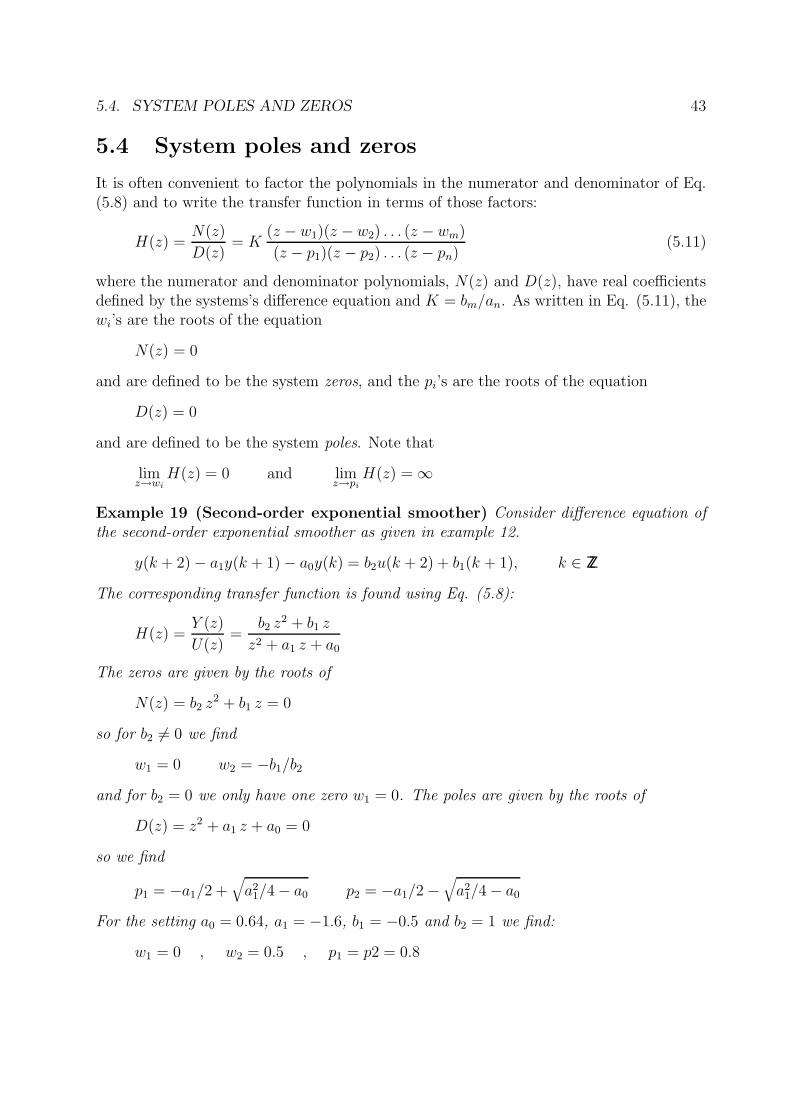
44 CHAPTER 5. THE DISCRETE-TIME TRANSFER FUNCTION
Figure 5.1: Pole-zero plot of a third order discrete-time system
Example 20 (Poles and zeros of third-order system)
Consider the third-order system in example 18, with transfer function
H(z) =100 z3 − 10 z2 + 48 z − 34
100 z3 − 180 z2 + 121 z − 41(5.12)
The poles of the system are finding the roots of the equation
D(z) = 100 z3 − 180 z2 + 121 z − 41 = 100(z − 1)(z − 0.4 − j 0.5)(z − 0.4 + j 0.5) = 0
We find that the poles are equal to p1 = 1, p2 = 0.4 + j 0.5 and p3 = 0.4− j 0.5. The zerosof the system are finding the roots of the equation
N(z) = 100 z3 − 10 z2 + 48 z − 34 = 100(z − 0.5)(z + 0.2 − j 0.8)(z + 0.2 + j 0.8) = 0
We find that the zeros are equal to p1 = 0.5, p2 = −0.2 + j 0.8 and p3 = −0.2 − j 0.8.
The pole-zero plot of this system is given in Fig. 5.1
5.4.1 System poles and the homogeneous response
Also in the discrete-time case there holds
The transfer function poles are the roots of the characteristic equationand also the eigenvalues of the system A matrix (as discussed in theprevious chapter).

5.4. SYSTEM POLES AND ZEROS 45
So let the transfer function denominator polynomial be given by
D(z) = an zn + an−1 z
n−1 + . . .+ a0
and let the roots of D(z) = 0 be given by pi, i = 1, . . . , n. Then the homogeneous responseof the system is given by
yh(k) =n∑
i=1
Ci pki
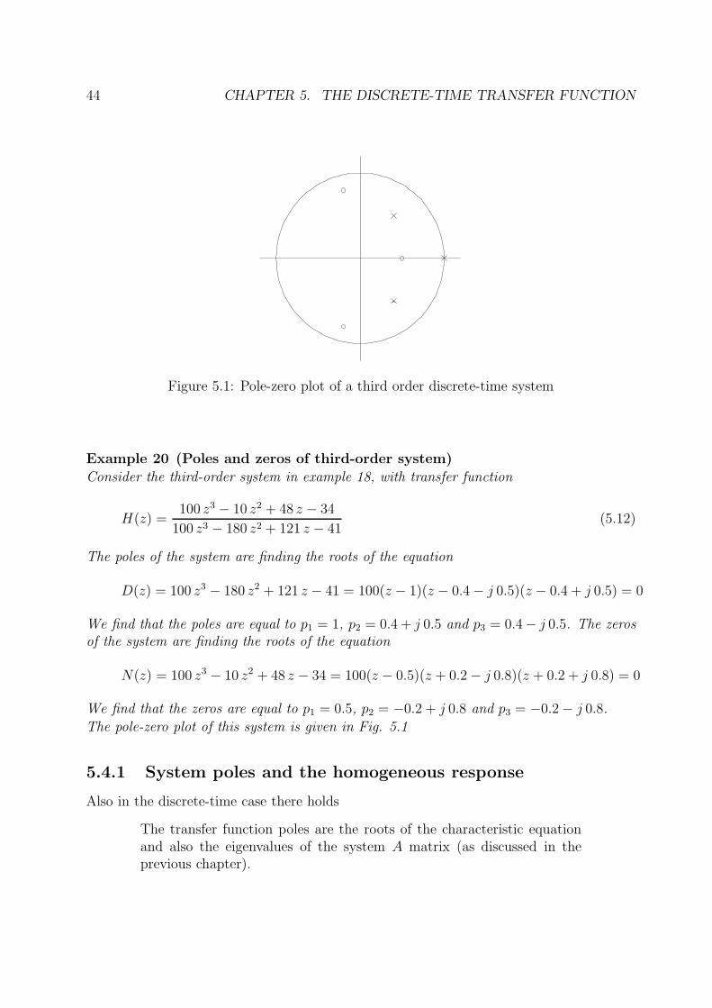
The location of the poles in the z-plane therefore determines the n components in thehomogeneous response as follows:
1. A real pole inside the unit circle (|p| < 1) defines an exponentially decaying compo-nent C pk in the homogeneous response. The rate is determined by the pole location;poles further away from the origin corresponds to components that decay rapidly;poles close to the origin correspond to slowly decaying components. Negative realpoles alternate in sign.
2. A pole in pi = 1 defines a component that is constant in amplitude and defined bythe initial conditions.
3. A real pole outside the unit circle (|p| > 1) corresponds to an exponentially increas-ing component C pk in the homogeneous response, thus defining the system to beunstable.
4. A complex conjugate pole pair p = ρ e±j ψ inside the unit circle combine to generatea response component that is decaying sinusoid of the form Aρk sin(ψ k + φ) whereA and φ are determined by the initial conditions. The rate of decaying is specifiedby ρ; The frequency of oscillation is determined by ψ.
5. A complex conjugate pole pair on the unit circle p = e±j ψ generates an oscillatorycomponent of the form A sin(ψ k + φ) where A and φ are determined by the initialconditions.
6. A complex pole pair outside the unit circle generates a exponentially increasing os-cillatory component.
5.4.2 System stability
A n-th order linear discrete-time system is asymptotically stable only if all componentsin the homogeneous response from a finite set of initial conditions decay to zero as timeincreases, or
limk→∞
n∑
i=1
Cipki = 0
where pi are the system poles. If any poles has magnitude larger than one, there is acomponent in the output without bound, causing the system to be unstable.
46 CHAPTER 5. THE DISCRETE-TIME TRANSFER FUNCTION
p = −1 p = 0 p = 0.5 p = 0.9
p = −0.9 p = 1.2
p = −0.5 p = 0.2 + j 0.8 p = ej 0.4 p = 1
��
�
QQQk
JJ
JJ
JJ
JJ
JJ]
��
� ?HHHHHj
���
������������
6
CCCCO
Figure 5.2: The specification of the form of components of the homogeneous response fromthe system pole locations on the pole-zero plot
5.4. SYSTEM POLES AND ZEROS 47
In order for a linear discrete-time system to be stable, all its poles musthave a magnitude strictly smaller than one, that is they must all lie insidethe unit circle. An “unstable” pole, lying outside the unit circle, gen-erates a component in the system homogeneous response that increaseswithout bound from any finite initial conditions. A system having oneor more poles lying on the unit circle has nondecaying oscillatory com-ponents in the homogeneous response and is defined to be marginallystable.
5.4.3 State space formulated systems
Consider the n-th order linear system describe by the set of n state equations and oneoutput equation:
x(k + 1) = Ax(k) +Bu(k) (5.13)
y(k) = Cx(k) +Du(k) (5.14)
The transfer function is given by
H(z) =Y (z)
U(z)
= [C (z I − A)−1B +D]
=C adj(z I −A)−1B +D det(z I −A)
det(z I − A)
Example 21 (Transfer function of a third-order system)Consider the third-order system in example 18. The state-space representation is foundusing the results of section 2.2:
A =
0 1 00 0 1
0.41 −1.21 1.8
B =
00
0.01
C =[
7 −73 170]
D = 1
We compute the adjoint of (z I −A):
adj(z I −A) =
z2 − 1.8 z + 1.21 0.41 0.41 zz − 1.8 z2 − 1.8 z −1.21 z + 0.41
1 z z2
and the determinant of (z I − A):
det(z I − A) = z3 − 1.8 z2 + 1.21 z − 0.41
and so:
H(z) =C adj(z I − A)−1B +D det(z I −A)
det(z I − A)
=z3 − 0.1 z2 + 0.48 z − 0.34
z3 − 1.80 z2 + 1.21 z − 0.41

48 CHAPTER 5. THE DISCRETE-TIME TRANSFER FUNCTION
Bibliography
[1] H. Freeman. Discrete-time systems. John Wiley & Sons, New York, USA, 1965.
[2] H. Kwakernaak and R. Sivan. Modern Signals and Systems. Prentice Hall, New Jersey,USA, 1991.
[3] C. Phillips and J.M. Parr. Signals, Systems, and Tranforms. Prentice Hall, New Jersey,USA, 1999.
[4] D. Rowell and D.N. Wormley. System Dynamics, an introduction. Prentice Hall, NewJersey, USA, 1997.
49


![DYNAMICS OF A DISCRETE-TIME STOICHIOMETRIC ...hwang/DiscreteOptimalForaging.pdfstoichiometric optimal foraging model [15] with its discrete-time analog. We study the discrete-time](https://img.dokumen.tips/doc/110x75/60c2e22ddd4f9278ff1214c6/dynamics-of-a-discrete-time-stoichiometric-hwangdiscreteoptimalforagingpdf.jpg)