Embed Size (px)
Citation preview
Journal of Machine Learning Research 16 (2015) 3079-3114 Submitted 1/15; Revised 3/15; Published 12/15
Discrete Reproducing Kernel Hilbert Spaces: Sampling andDistribution of Dirac-masses
Palle Jorgensen [email protected] of MathematicsThe University of IowaIowa City, IA 52242-1419, U.S.A.
Feng Tian [email protected]
Department of Mathematics, Informatics, and Cybersecurity
Trine University
Angola, IN 46703, U.S.A.
Editor: John Shawe-Taylor
Abstract
We study reproducing kernels, and associated reproducing kernel Hilbert spaces (RKHSs)H over infinite, discrete and countable sets V . In this setting we analyze in detail thedistributions of the corresponding Dirac point-masses of V . Illustrations include certainmodels from neural networks: An Extreme Learning Machine (ELM) is a neural network-configuration in which a hidden layer of weights are randomly sampled, and where theobject is then to compute resulting output. For RKHSs H of functions defined on aprescribed countable infinite discrete set V , we characterize those which contain the Diracmasses δx for all points x in V . Further examples and applications where this questionplays an important role are: (i) discrete Brownian motion-Hilbert spaces, i.e., discreteversions of the Cameron-Martin Hilbert space; (ii) energy-Hilbert spaces corresponding tograph-Laplacians where the set V of vertices is then equipped with a resistance metric; andfinally (iii) the study of Gaussian free fields.
Keywords: Gaussian reproducing kernel Hilbert spaces, sampling in discrete systems,resistance metric, graph Laplacians, discrete Green’s functions
1. Introduction
A reproducing kernel Hilbert space (RKHS) is a Hilbert space H of functions on a pre-scribed set, say V , with the property that point-evaluation for functions f ∈H is continu-ous with respect to the H -norm. They are called kernel spaces, because, for every x ∈ V ,the point-evaluation for functions f ∈H , f (x) must then be given as a H -inner productof f and a vector kx, in H ; called the kernel.
The RKHSs have been studied extensively since the pioneering papers by Aronszajn(1943; 1948). They further play an important role in the theory of partial differential oper-ators (PDO); for example as Green’s functions of second order elliptic PDOs (Nelson, 1957;Haeseler et al., 2014). Other applications include engineering, physics, machine-learningtheory (Kulkarni and Harman, 2011; Smale and Zhou, 2009; Cucker and Smale, 2002),stochastic processes (Alpay and Dym, 1993; Alpay et al., 1993; Alpay and Dym, 1992; Al-pay et al., 2013, 2014), numerical analysis, and more (Lin and Brown, 2004; Ha Quang et al.,
c©2015 Palle Jorgensen and Feng Tian.
Jorgensen and Tian
2010; Zhang et al., 2012; Lata and Paulsen, 2011; Vuletic, 2013; Schramm and Sheffield,2013; Hedenmalm and Nieminen, 2014; Shawe-Taylor and Cristianini, 2004; Schlkopf andSmola, 2001). But the literature so far has focused on the theory of kernel functions definedon continuous domains, either domains in Euclidean space, or complex domains in one ormore variables. For these cases, the Dirac δx distributions do not have finite H -norm. Butfor RKHSs over discrete point distributions, it is reasonable to expect that the Dirac δxfunctions will in fact have finite H -norm.
An illustration from neural networks: An Extreme Learning Machine (ELM) is a neuralnetwork configuration in which a hidden layer of weights are randomly sampled (Rasmussenand Williams, 2006), and the object is then to determine analytically resulting output layerweights. Hence ELM may be thought of as an approximation to a network with infinitenumber of hidden units.
Here we consider the discrete case, i.e., RKHSs of functions defined on a prescribedcountable infinite discrete set V . We are concerned with a characterization of those RKHSsH which contain the Dirac masses δx for all points x ∈ V . Of the examples and applicationswhere this question plays an important role, we emphasize three: (i) discrete Brownianmotion-Hilbert spaces, i.e., discrete versions of the Cameron-Martin Hilbert space; (ii)energy-Hilbert spaces corresponding to graph-Laplacians; and finally (iii) RKHSs generatedby binomial coefficients. We show that the point-masses have finite H -norm in cases (i)and (ii), but not in case (iii).
Our setting is a given positive definite function k on V × V , where V is discrete. Westudy the corresponding RKHS H (= H (k)) in detail. Our main results are Theorems 1,2, and 3 which give explicit answers to the question of which point-masses from V are inH . Applications include Corollaries 29, 41, 46, 48, 52, and 53.
The paper is organized as follows: Section 2 leads up to our characterization (Theorem1) of point-masses which have finite H -norm. It is applied in Sections 3 and 4 to a varietyof classes of discrete RKHSs. Section 3 deals with samples from Brownian motion, andfrom the Brownian bridge process, and binomial kernels, and with kernels on sets V × Vwhich arise as restrictions to sample-points. Section 4 covers the case of infinite networkof resistors. By this we mean an infinite graph with assigned resistors on its edges. Inthis family of examples, the associated RKHSs vary with the assignment of resistors on theedges in G, and are computed explicitly from a resulting energy form. Our result Corollary46 states that, for the network models, all point-masses have finite energy. Furthermore, wecompute the value, and we study V as a metric space w.r.t. the corresponding resistancemetric. These results, in turn, have direct implications (Corollaries 48, 52 and 55) for thefamily of Gaussian free fields associated with our infinite network models.
A positive definite kernel k is said to be universal (Steinwart, 2002; Caponnetto et al.,2008) if, every continuous function, on a compact subset of the input space, can be uniformlyapproximated by sections of the kernel, i.e., by continuous functions in the RKHS. InTheorem 3 we show that for the RKHSs from kernels kc in electrical network G of resistors,this universality holds. The metric in this case is the resistance metric on the vertices of G,determined by the assignment of a conductance function c on the edges in G.
Infinite vs finite graphs. We study “large weighted graphs” (vertices V , edges E, andweights as functions assigned on the edges E), and our motivation derives from learningwhere “learning” is understood broadly to include (machine) learning of suitable probability
3080
Discrete Reproducing Kernel Hilbert Spaces
distribution, i.e., meaning learning from samples of training data. Other applications of ananalysis of weighted graphs include statistical mechanics, such as infinite spin models, andlarge digital networks. It is natural to ask then how one best approaches analysis on “large”systems. We propose an analysis via infinite weighted graphs. This is so even if some ofthe questions in learning theory may in fact refer to only “large” finite graphs.
One reason for this (among others) is that statistical features in such an analysis arebest predicted by consideration of probability spaces corresponding to measures on infinitesample spaces. Moreover the latter are best designed from consideration of infinite weightedgraphs, as opposed to their finite counterparts. Examples of statistical features which arerelevant even for finite samples is long-range order; i.e., the study of correlations betweendistant sites (vertices), and related phase-transitions, e.g., sign-flips at distant sites. Indesigning efficient learning models, it is important to understand the possible occurrenceof unexpected long-range correlations; e.g., correlations between distant sites in a finitesample.
A second reason for the use of infinite sample-spaces is their use in designing efficientsampling procedures. The interesting solutions will often occur first as vectors in an infinite-dimensional reproducing-kernel Hilbert space RKHS. Indeed, such RKHSs serve as powerfultools in the solution of a kernel-optimization problems with penalty terms. Once an optimalsolution is obtained in infinite dimensions, one may then proceed to study its restrictionsto suitably chosen finite subgraphs.
In general when reproducing kernels and their Hilbert spaces are used, one ends up withfunctions on a suitable set, and so far we feel that the dichotomy discrete vs continuoushas not yet received sufficient attention. After all, a choice of sampling points in relevantoptimization models based on kernel theory suggests the need for a better understandingof point masses as they are accounted for in the RKHS at hand. In broad outline, this is aleading theme in our paper.
2. Discrete RKHSs
Definition 1 Let V be a countable and infinite set, and F (V ) the set of all finite subsetsof V . A function k : V × V → C is said to be positive definite, if∑∑
(x,y)∈F×F
k (x, y) cxcy ≥ 0 (1)
holds for all coefficients cxx∈F ⊂ C, and all F ∈ F (V ).
Definition 2 Fix a set V , countable infinite.
1. For all x ∈ V , setkx := k (·, x) : V → C (2)
as a function on V .
2. Let H := H (k) be the Hilbert-completion of the span kx : x ∈ V , with respect tothe inner product ⟨∑
cxkx,∑
dyky
⟩H
:=∑∑
cxdyk (x, y) (3)
3081
Jorgensen and Tian
modulo the subspace of functions of zero H -norm. H is then a reproducing kernelHilbert space (HKRS), with the reproducing property:
〈kx, ϕ〉H = ϕ (x) , ∀x ∈ V, ∀ϕ ∈H . (4)
Note. The summations in (3) are all finite. Starting with finitely supported summa-tions in (3), the RKHS H = H (k) is then obtained by Hilbert space completion. Weuse physicists’ convention, so that the inner product is conjugate linear in the firstvariable, and linear in the second variable.
3. If F ∈ F (V ), set HF = closed spankxx∈F ⊂ H , (closed is automatic if F isfinite.) And set
PF := the orthogonal projection onto HF . (5)
4. For F ∈ F (V ), setKF := (k (x, y))(x,y)∈F×F (6)
as a #F ×#F matrix.
Remark 3 It follows from the above that reproducing kernel Hilbert spaces (RKHS) arisefrom a given positive definite kernel k, a corresponding pre-Hilbert form; and then a Hilbert-completion. The question arises: “What are the functions in the completion?” Now, beforecompletion, the functions are as specified in Definition 2, but the Hilbert space completionsare subtle; they are classical Hilbert spaces of functions, not always transparent from thenaked kernel k itself. Examples of classical RKHSs: Hardy spaces or Bergman spaces (forcomplex domains), Sobolev spaces and Dirichlet spaces (Okoudjou et al., 2013; Strichartzand Teplyaev, 2012; Strichartz, 2010) (for real domains, or for fractals), band-limited L2
functions (from signal analysis), and Cameron-Martin Hilbert spaces from Gaussian pro-cesses (in continuous time domain).
Our focus here is on discrete analogues of the classical RKHSs from real or complexanalysis. These discrete RKHSs in turn are dictated by applications, and their features arequite different from those of their continuous counterparts.
Definition 4 The RKHS H = H (k) is said to have the discrete mass property (H is
called a discrete RKHS), if δx ∈ H , for all x ∈ V . Here, δx (y) =
1 if x = y
0 if x 6= y, i.e., the
Dirac mass at x ∈ V .
Lemma 5 Let F ∈ F (V ), x1 ∈ F . Assume δx1 ∈H . Then
PF (δx1) (·) =∑y∈F
(K−1F δx1
)(y) ky (·) . (7)
Proof Show thatδx1 −
∑y∈F
(K−1F δx1
)(y) ky (·) ∈H ⊥
F . (8)
The remaining part follows easily from this.
3082
Discrete Reproducing Kernel Hilbert Spaces
(The notation (HF )⊥ stands for orthogonal complement, also denoted H HF =ϕ ∈H
∣∣ 〈f, ϕ〉H = 0, ∀f ∈HF
.)
Lemma 6 Using Dirac’s bra-ket, and ket-bra notation (for rank-one operators), the orthog-onal projection onto HF is
PF =∑y∈F
∣∣ky 〉〈 k∗y∣∣ ; (9)
where
k∗x :=∑y∈F
(K−1F
)yxky (10)
is the dual vector to kx, for all x ∈ V .
Proof Let k∗x be specified as in (10), then
〈k∗x, kz〉H =∑y∈F
⟨(K−1F
)yxky, kz
⟩H
=∑y∈F
(K−1F
)xy〈ky, kz〉H
=∑y∈F
(K−1F
)xy
(KF )yz = δx,z,
i.e., k∗x is the dual vector to kx, for all x ∈ V .
For f ∈H , and F ∈ F (V ), we have∑y∈F
∣∣ky 〉〈 k∗y∣∣ f =∑y∈F
⟨k∗y, f
⟩Hky
=∑∑
(y,z)∈F×F
(K−1F
)z,y〈kz, f〉H
= PF f.
This yields the orthogonal projection realized as stated in (9).
Now, applying (9) to δx1 , we get
PF (δx1) =∑y∈F
⟨k∗y, δx1
⟩Hky
=∑y∈F
(∑z∈F
(K−1F
)yz〈kz, δx1〉H
)ky
=∑y∈F
(∑z∈F
(K−1F
)yzδx1 (z)
)ky
=∑y∈F
(K−1F δx1
)(y) ky,
3083
Jorgensen and Tian
where (K−1F δx1
)(y) :=
∑z∈F
(K−1F
)yzδx1 (z) .
This verifies (7).
Remark 7 Note a slight abuse of notations: We make formally sense of the expressions forPF (δx) in (7) even in the case when δx might not be in H . For all finite F , we showed thatPF (δx) ∈ H . But for δx be in H , we must have the additional boundedness assumption(18) satisfied; see Theorem 1.
Lemma 8 Let F ∈ F (V ), x1 ∈ F , then(K−1F δx1
)(x1) = ‖PF δx1‖
2H . (11)
Proof Setting ζ(F ) := K−1F (δx1), we have
PF (δx1) =∑y∈F
ζ(F ) (y) kF (·, y)
and for all z ∈ F ,∑z∈F
ζ(F ) (z)PF (δx1) (z)︸ ︷︷ ︸ζ(F )(x1)
=∑F
∑F
ζ(F ) (z) ζ(F ) (y) kF (z, y) (12)
= ‖PF δx1‖2H .
By Lemma 6, the LHS of (12) is given by
‖PF δx1‖2H = 〈PF δx1 , δx1〉H
=∑y∈F
(K−1F δx1
)(y) 〈ky, δx1〉H
=(K−1F δx1
)(x1) = K−1
F (x1, x1) .
Corollary 9 If δx1 ∈H (see Theorem 1), then
supF∈F (V )
(K−1F δx1
)(x1) = ‖δx1‖
2H . (13)
The following condition is satisfied in some examples, but not all:
Corollary 10 ∃F ∈ F (V ) s.t. δx1 ∈HF ⇐⇒
K−1F ′ (δx1) (x1) = K−1
F (δx1) (x1)
for all F ′ ⊃ F .
3084
Discrete Reproducing Kernel Hilbert Spaces
Corollary 11 (Monotonicity) If F and F ′ are in F (V ) and F ⊂ F ′, then(K−1F δx1
)(x1) ≤
(K−1F ′ δx1
)(x1) (14)
and
limFV
(K−1F δx1
)(x1) = ‖δx1‖
2H . (15)
Proof By (11), (K−1F δx1
)(x1) = ‖PF δx1‖
2H .
Since HF ⊂HF ′ , we have PFPF ′ = PF , so
‖PF δx1‖2H = ‖PFPF ′δx1‖
2H ≤ ‖PF ′δx1‖
2H
i.e., (K−1F δx1
)(x1) ≤
(K−1F ′ δx1
)(x1) .
So (14) follows; and the limit in (15) is monotone.
Theorem 1 Given V , k : V × V → R positive definite (p.d.). Let H = H (k) be the cor-responding RKHS. Assume V is countable and infinite. Then the following three conditions(i)-(iii) are equivalent; x1 ∈ V is fixed:
(i) δx1 ∈H ;
(ii) ∃Cx1 <∞ such that for all F ∈ F (V ), the following estimate holds:
|ξ (x1)|2 ≤ Cx1∑∑F×F
ξ (x)ξ (y) k (x, y) (16)
(iii) For F ∈ F (V ), set
KF = (k (x, y))(x,y)∈F×F (17)
as a #F ×#F matrix. Then
supF∈F (V )
(K−1F δx1
)(x1) <∞. (18)
Proof (i)⇒(ii) For ξ ∈ l2 (F ), set
hξ =∑y∈F
ξ (y) ky (·) ∈HF .
Then 〈δx1 , hξ〉H = ξ (x1) for all ξ.Since δx1 ∈H , then by Schwarz:∣∣〈δx1 , hξ〉H ∣∣2 ≤ ‖δx1‖2H ∑∑
F×Fξ (x)ξ (y) k (x, y) . (19)
3085
Jorgensen and Tian
But 〈δx1 , ky〉H = δx1,y =
1 y = x1
0 y 6= x1
; hence 〈δx1 , hξ〉H = ξ (x1), and so (19) implies (16).
(ii)⇒(iii) Recall the matrix
KF := (〈kx, ky〉)(x,y)∈F×F
as a linear operator l2 (F )→ l2 (F ), where
(KFϕ) (x) =∑y∈F
KF (x, y)ϕ (y) , ϕ ∈ l2 (F ) . (20)
By (16), we have
ker (KF ) ⊂ϕ ∈ l2 (F ) : ϕ (x1) = 0
. (21)
Equivalently,
ker (KF ) ⊂ δx1⊥ (22)
and so δx1
∣∣∣F∈ ker (KF )⊥ = ran (KF ), and ∃ ζ(F ) ∈ l2 (F ) s.t.
δx1
∣∣∣F
=∑y∈F
ζ(F ) (y) k (·, y)︸ ︷︷ ︸=:hF
. (23)
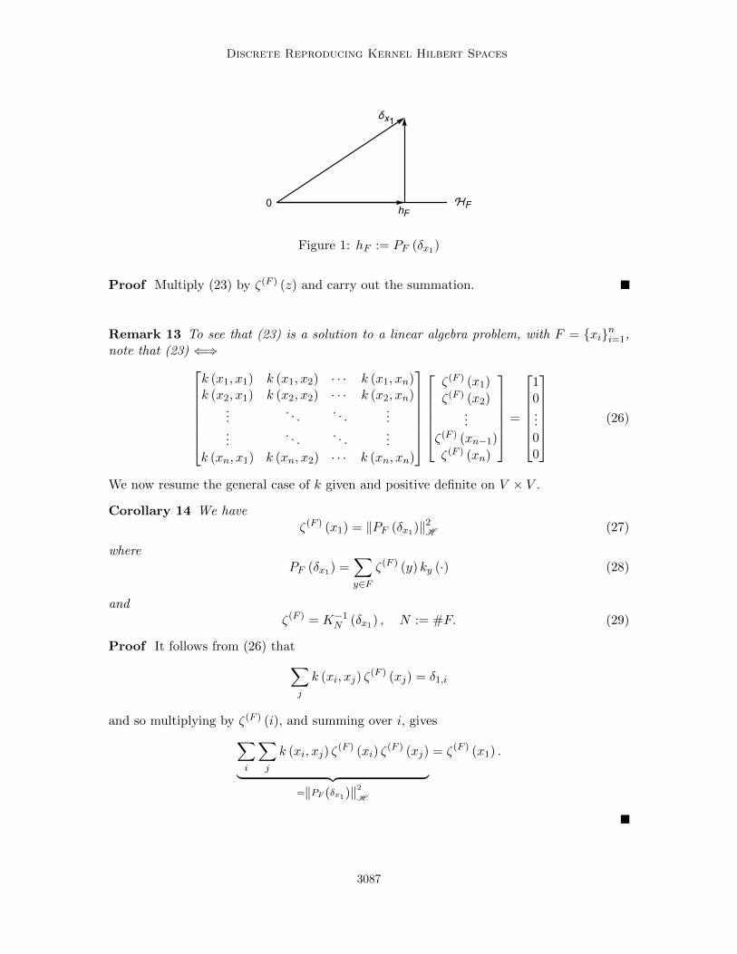
Claim. PF (δx1) = hF , where PF = projection onto HF ; see (5) and Lemma 5. (See Figure1.) Indeed, we only need to prove that δx1 − hF ∈H HF , i.e.,
〈δx1 − hF , kz〉H = 0, ∀z ∈ F. (24)
But, by (23),
LHS(24) = δx1,z −∑y∈F
k (z, y) ζ(F ) (y) = 0.
This proves the claim.
If F ⊂ F ′, F, F ′ ∈ F (V ), then HF ⊂ HF ′ , and PFPF ′ = PF by easy facts forprojections. Hence
‖PF δx1‖2H ≤ ‖PF ′δx1‖
2H , hF := PF (δx1)
and
limFV
‖δx1 − hF ‖H = 0.
(iii)⇒(i) Follows from Lemma 8 and Corollary 9.
Corollary 12 The numbers(ζ(F ) (y)
)y∈F in (23) satisfies
ζ(F ) (x1) =∑∑
(y,z)∈F×F
ζ(F ) (y) ζ(F ) (z) k (y, z) . (25)
3086
Discrete Reproducing Kernel Hilbert Spaces
0
δx1
hFℋF
Figure 1: hF := PF (δx1)
Proof Multiply (23) by ζ(F ) (z) and carry out the summation.
Remark 13 To see that (23) is a solution to a linear algebra problem, with F = xini=1,note that (23) ⇐⇒
k (x1, x1) k (x1, x2) · · · k (x1, xn)k (x2, x1) k (x2, x2) · · · k (x2, xn)
.... . .
. . ....
.... . .
. . ....
k (xn, x1) k (xn, x2) · · · k (xn, xn)
ζ(F ) (x1)
ζ(F ) (x2)...
ζ(F ) (xn−1)
ζ(F ) (xn)
=
10...00
(26)
We now resume the general case of k given and positive definite on V × V .
Corollary 14 We haveζ(F ) (x1) = ‖PF (δx1)‖2H (27)
wherePF (δx1) =
∑y∈F
ζ(F ) (y) ky (·) (28)
andζ(F ) = K−1
N (δx1) , N := #F. (29)
Proof It follows from (26) that∑j
k (xi, xj) ζ(F ) (xj) = δ1,i
and so multiplying by ζ(F ) (i), and summing over i, gives∑i
∑j
k (xi, xj) ζ(F ) (xi) ζ
(F ) (xj)︸ ︷︷ ︸=‖PF (δx1)‖2
H
= ζ(F ) (x1) .
3087
Jorgensen and Tian
Corollary 15 We have
(i)
PF (δx1) = ζ(F ) (x1) kx1 +∑
y∈F\x1
ζ(F ) (y) ky (30)
where ζF solves (26), for all F ∈ F (V );
(ii)
‖PF (δx1)‖2H = ζ(F ) (x1) (31)
and so in particular:
(iii)
0 < ζ(F ) (x1) ≤ ‖δx1‖2H (32)
Proof Formula (31) follows from the definition of ζ(F ) as a solution to the matrix problemKNζ
(F ) = δx1 , but we may also prove (31) directly from
PF (δx1) =∑y
ζ(F ) (y) ky . (33)
Apply 〈·, δx1〉H to both sides in (33), we get
〈δx1 , PF (δx1)〉H︸ ︷︷ ︸‖PF (δx1)‖2
H
= ζ(F ) (x1)
since PF = P ∗F = P 2F ; i.e., a projection in the RKHS H = HV of k.
Example 1 (#F = 2) Let F = x1, x2, KF = (kij)2i,j=1, where kij := k (xi, xj). Then
(26) reads [k11 k12
k21 k22
] [ζF (x1)ζF (x2)
]=
[10
]. (34)
Set D := det (KF ) = k11k22 − k12k21, then:
ζF (x1) =k22
D, ζF (x2) = −k21
D.
Example 2 Let V = x1, x2, . . . be an ordered set. Set Fn := x1, . . . , xn. Note that with
Dn = det (KFn) = det(
(k (xi, xj))ni,j=1
), and (35)
D′n−1 = (1, 1) minor of KFn = det(
(k (xi, xj))ni,j=2
); (36)
then
ζ(Fn) (x1) =D′n−1
Dn=(K−1Fnδx1)
(x1) . (37)
3088
Discrete Reproducing Kernel Hilbert Spaces
Corollary 16 We have
1
k (x1, x1)≤ k (x2, x2)
D2≤ · · · ≤
D′n−1
Dn≤ · · · ≤ ‖δx1‖
2H .
Proof Follows from (37), and if F ⊂ F ′ are two finite subsets, then
‖PF (δx1)‖2H ≤ ‖PF ′ (δx1)‖2H ≤ ‖δx1‖2H .
Let k : V × V → R be as specified above. Let H = H (k) be the RKHS. We set F (V ):=all finite subsets of V ; and if x ∈ V is fixed, Fx (V ) := F ∈ F (V ) | x ∈ F.
For F ∈ F (V ), let KF be the #F ×#F matrix given by (k (x, y))(x,y)∈F×F . FollowingKarlin and Ziegler (1996), we say that k is strictly positive iff detKF > 0 for all F ∈ F (V ).
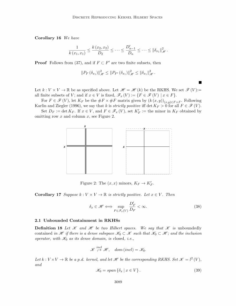
Set DF := detKF . If x ∈ V , and F ∈ Fx (V ), set K ′F := the minor in KF obtained byomitting row x and column x, see Figure 2.
x
x
x
x
Figure 2: The (x, x) minors, KF → K ′F .
Corollary 17 Suppose k : V × V → R is strictly positive. Let x ∈ V . Then
δx ∈H ⇐⇒ supF∈Fx(V )
D′FDF
<∞. (38)
2.1 Unbounded Containment in RKHSs
Definition 18 Let K and H be two Hilbert spaces. We say that K is unboundedlycontained in H if there is a dense subspace K0 ⊂ K such that K0 ⊂H ; and the inclusionoperator, with K0 as its dense domain, is closed, i.e.,
Kincl→ H , dom (incl) = K0.
Let k : V ×V → R be a p.d. kernel, and let H be the corresponding RKHS. Set K = l2 (V ),and
K0 = span δx | x ∈ V . (39)
3089
Jorgensen and Tian
Proposition 19 If δx ∈H for ∀x ∈ V , then l2 (V ) is unboundedly contained in H .
Proof Recall that H is the RKHS defined for a fixed p.d. kernel k : V × V → R. Let kxbe the vector in H , given by kx (y) = k (x, y), s.t.
f (x) = 〈kx, f〉H , ∀f ∈H . (40)
To finish the proof we will need:
Lemma 20 The following equation
〈δx, ky〉H = δx,y (41)
holds if δx ∈H for ∀x ∈ V .
Proof (41) is immediate from (40).
Lemma 21 Onspan kx | x ∈ V ⊂H (42)
define Mkx := δx, then by Lemma 20, M extends to be a well defined operator M : H →l2 (V ) with dense domain (42). We have
〈k,Mf〉l2(V ) = 〈k, f〉H , ∀k ∈ span δx , ∀f ∈ dom (M) . (43)
Proof By linearity, it is enough to prove that
〈δx, δy〉l2 = 〈δx, ky〉H (44)
holds for ∀x, y ∈ V . But (44) follows immediate from Lemma 20.
Corollary 22 If L : l2 (V )→H denotes the inclusion mapping with
dom (L) = span δx : x ∈ V ,
then we conclude thatL ⊂M∗, and M ⊂ L∗. (45)
Since dom (M) is dense in H , it follows that L∗ has dense domain; and that therefore Lis closable.
Remark 23 This also completes the proof of Proposition 19.
Corollary 24 Suppose k : V ×V → R is as given, and that H = RKHS (k). Let L be thedensely defined inclusion mapping l2 (V )→H . Then L∗L is selfadjoint with dense domainin l2 (V ); and LL∗ is selfadjoint with dense domain in H . Moreover, the following polardecomposition holds:
L = U (L∗L)1/2 = (LL∗)1/2 U (46)
where U is a partial isometry l2 (V )→H .
3090
Discrete Reproducing Kernel Hilbert Spaces
3. Point-masses in Concrete Models
Suppose V ⊂ D ⊂ Rd where V is countable and discrete, but D is open. In this case, weget two kernels: k on D × D, and kV := k
∣∣V×V on V × V by restriction. If x ∈ V , then
k(V )x (·) = k (·, x) is a function on V , while kx (·) = k (·, x) is a function on D.
This means that the corresponding RKHSs are different, HV vs H , where HV = aRKHS of functions on V , and H = a RKHS of functions on D.
Lemma 25 HV is isometrically contained in H via k(V )x 7−→ kx, x ∈ V .
Proof If F ⊂ V is a finite subset, and ξ = ξF is a function on F , then∥∥∥∑x∈F
ξ (x) k(V )x
∥∥∥HV
=∥∥∥∑
x∈Fξ (x) kx
∥∥∥H.
The desired result follows from this.
We are concerned with cases of kernels k : D ×D → R with restriction kV : V × V → R,where V is a countable discrete subset of D. Typically, for x ∈ V , we may have (restriction)δx∣∣V∈HV , but δx /∈H ; indeed this happens for the kernel k of standard Brownian motion:
D = R+;V = an ordered subset 0 < x1 < x2 < · · · < xi < xi+1 < · · · , V = xi∞i=1.In this case, we compute HV , and we show that δxi
∣∣V∈ HV ; while for Hm = the
Cameron-Martin Hilbert space, we have δxi /∈Hm.Also note that δx1 has a different meaning with reference to HV vs Hm. In the first case,
it is simply δx1 (y) =
1 y = x1
0 y ∈ V \ x1. In the second case, δx1 is a Schwartz distribution.
We shall abuse notation, writing δx in both cases.In the following, we will consider restriction to V ×V of a special continuous p.d. kernel
k on R+ × R+. It is k (s, t) = s ∧ t = min (s, t). Before we restrict, note that the RKHS ofthis k is the Cameron-Martin Hilbert space of function f on R+ with distribution derivativef ′ ∈ L2 (R+), and
‖f‖2H :=
∫ ∞0
∣∣f ′ (t)∣∣2 dt <∞. (47)
For details, see below.
Remark 26 (Application) The Hilbert space given by ‖·‖2H in (47) is called the Cameron-Martin Hilbert space, and, as noted, it is the RKHS of k : R+ × R+ → R : k (s, t) := s ∧ t.Now pick a discrete subset V ⊂ R+; then Lemma 25 states that the RKHS of the V × Vrestricted kernel, k(V ) is isometrically embedded into H , i.e., setting
J (V )(k(V )x
)= kx, ∀x ∈ V ; (48)
J (V ) extends by “closed span” to an isometry HVJ(V )
−−−→ H . It further follows from thelemma, that the range of J (V ) may have infinite co-dimension.
Note that PV := J (V )(J (V )
)∗is the projection onto the range of J (V ). The ortho-
complement is as follow:
H HV =ψ ∈H
∣∣ ψ (x) = 0, ∀x ∈ V. (49)
3091
Jorgensen and Tian
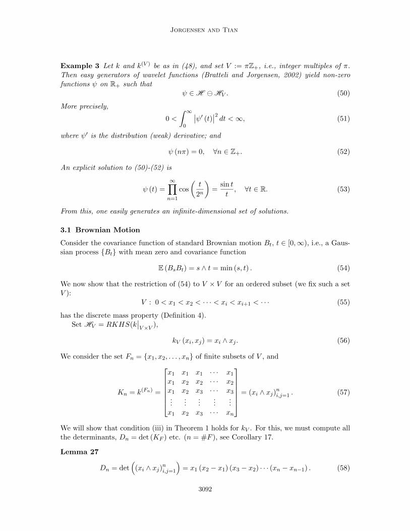
Example 3 Let k and k(V ) be as in (48), and set V := πZ+, i.e., integer multiples of π.Then easy generators of wavelet functions (Bratteli and Jorgensen, 2002) yield non-zerofunctions ψ on R+ such that
ψ ∈H HV . (50)
More precisely,
0 <
∫ ∞0
∣∣ψ′ (t)∣∣2 dt <∞, (51)
where ψ′ is the distribution (weak) derivative; and
ψ (nπ) = 0, ∀n ∈ Z+. (52)
An explicit solution to (50)-(52) is
ψ (t) =
∞∏n=1
cos
(t
2n
)=
sin t
t, ∀t ∈ R. (53)
From this, one easily generates an infinite-dimensional set of solutions.
3.1 Brownian Motion
Consider the covariance function of standard Brownian motion Bt, t ∈ [0,∞), i.e., a Gaus-sian process Bt with mean zero and covariance function
E (BsBt) = s ∧ t = min (s, t) . (54)
We now show that the restriction of (54) to V × V for an ordered subset (we fix such a setV ):
V : 0 < x1 < x2 < · · · < xi < xi+1 < · · · (55)
has the discrete mass property (Definition 4).Set HV = RKHS(k
∣∣V×V ),
kV (xi, xj) = xi ∧ xj . (56)
We consider the set Fn = x1, x2, . . . , xn of finite subsets of V , and
Kn = k(Fn) =
x1 x1 x1 · · · x1
x1 x2 x2 · · · x2
x1 x2 x3 · · · x3...
......
......
x1 x2 x3 · · · xn
= (xi ∧ xj)ni,j=1 . (57)
We will show that condition (iii) in Theorem 1 holds for kV . For this, we must compute allthe determinants, Dn = det (KF ) etc. (n = #F ), see Corollary 17.
Lemma 27
Dn = det(
(xi ∧ xj)ni,j=1
)= x1 (x2 − x1) (x3 − x2) · · · (xn − xn−1) . (58)
3092
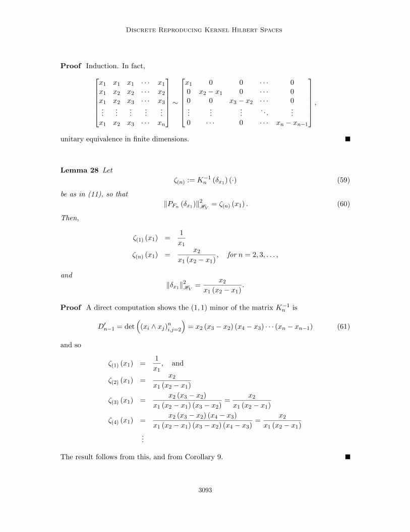
Discrete Reproducing Kernel Hilbert Spaces
Proof Induction. In fact,x1 x1 x1 · · · x1
x1 x2 x2 · · · x2
x1 x2 x3 · · · x3...
......
......
x1 x2 x3 · · · xn
∼x1 0 0 · · · 00 x2 − x1 0 · · · 00 0 x3 − x2 · · · 0...
......
. . ....
0 · · · 0 · · · xn − xn−1
,
unitary equivalence in finite dimensions.
Lemma 28 Let
ζ(n) := K−1n (δx1) (·) (59)
be as in (11), so that
‖PFn (δx1)‖2HV= ζ(n) (x1) . (60)
Then,
ζ(1) (x1) =1
x1
ζ(n) (x1) =x2
x1 (x2 − x1), for n = 2, 3, . . . ,
and
‖δx1‖2HV
=x2
x1 (x2 − x1).
Proof A direct computation shows the (1, 1) minor of the matrix K−1n is
D′n−1 = det(
(xi ∧ xj)ni,j=2
)= x2 (x3 − x2) (x4 − x3) · · · (xn − xn−1) (61)
and so
ζ(1) (x1) =1
x1, and
ζ(2) (x1) =x2
x1 (x2 − x1)
ζ(3) (x1) =x2 (x3 − x2)
x1 (x2 − x1) (x3 − x2)=
x2
x1 (x2 − x1)
ζ(4) (x1) =x2 (x3 − x2) (x4 − x3)
x1 (x2 − x1) (x3 − x2) (x4 − x3)=
x2
x1 (x2 − x1)
...
The result follows from this, and from Corollary 9.
3093
Jorgensen and Tian
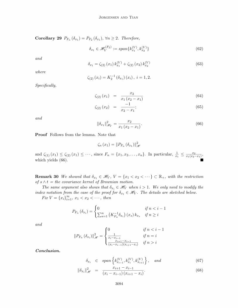
Corollary 29 PFn (δx1) = PF2 (δx1), ∀n ≥ 2. Therefore,
δx1 ∈H(F2)V := spank(V )
x1 , k(V )x2 (62)
and
δx1 = ζ(2) (x1) k(V )x1 + ζ(2) (x2) k(V )
x2 (63)
where
ζ(2) (xi) = K−12 (δx1) (xi) , i = 1, 2.
Specifically,
ζ(2) (x1) =x2
x1 (x2 − x1)(64)
ζ(2) (x2) =−1
x2 − x1; (65)
and
‖δx1‖2HV
=x2
x1 (x2 − x1). (66)
Proof Follows from the lemma. Note that
ζn (x1) = ‖PFn (δx1)‖2H
and ζ(1) (x1) ≤ ζ(2) (x1) ≤ · · · , since Fn = x1, x2, . . . , xn. In particular, 1x1≤ x2
x1(x2−x1) ,
which yields (66).
Remark 30 We showed that δx1 ∈ HV , V = x1 < x2 < · · · ⊂ R+, with the restrictionof s ∧ t = the covariance kernel of Brownian motion.
The same argument also shows that δxi ∈HV when i > 1. We only need to modify theindex notation from the case of the proof for δx1 ∈HV . The details are sketched below.
Fix V = xi∞i=1, x1 < x2 < · · · , then
PFn (δxi) =
0 if n < i− 1∑n
s=1
(K−1Fnδxi)
(xs) kxs if n ≥ i
and
‖PFn (δxi)‖2H =
0 if n < i− 1
1xi−xi−1
if n = ixi+1−xi−1
(xi−xi−1)(xi+1−xi) if n > i
Conclusion.
δxi ∈ spank(V )xi−1
, k(V )xi , k
(V )xi+1
, and (67)
‖δxi‖2H =
xi+1 − xi−1
(xi − xi−1) (xi+1 − xi). (68)
3094
Discrete Reproducing Kernel Hilbert Spaces
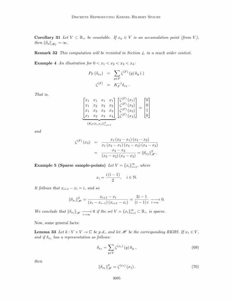
Corollary 31 Let V ⊂ R+ be countable. If xa ∈ V is an accumulation point (from V ),then ‖δa‖HV
=∞.
Remark 32 This computation will be revisited in Section 4, in a much wider context.
Example 4 An illustration for 0 < x1 < x2 < x3 < x4:
PF (δx3) =∑y∈F
ζ(F ) (y) ky (·)
ζ(F ) = K−1F δx3 .
That is, x1 x1 x1 x1
x1 x2 x2 x2
x1 x2 x3 x3
x1 x2 x3 x4
︸ ︷︷ ︸
(KF (xi,xj))4i,j=1
ζ(F ) (x1)
ζ(F ) (x2)
ζ(F ) (x3)
ζ(F ) (x4)
=
0010
and
ζ(F ) (x3) =x1 (x2 − x1) (x4 − x2)
x1 (x2 − x1) (x3 − x2) (x4 − x3)
=x4 − x2
(x3 − x2) (x4 − x3)= ‖δx3‖
2H .
Example 5 (Sparse sample-points) Let V = xi∞i=1, where
xi =i (i− 1)
2, i ∈ N.
It follows that xi+1 − xi = i, and so
‖δxi‖2H =
xi+1 − xi(xi − xi−1) (xi+1 − xi)
=2i− 1
(i− 1) i−−−→i→∞
0.
We conclude that ‖δxi‖H −−−→i→∞0 if the set V = xi∞i=1 ⊂ R+ is sparse.
Now, some general facts:
Lemma 33 Let k : V × V → C be p.d., and let H be the corresponding RKHS. If x1 ∈ V ,and if δx1 has a representation as follows:
δx1 =∑y∈V
ζ(x1) (y) ky , (69)
then
‖δx1‖2H = ζ(x1) (x1) . (70)
3095
Jorgensen and Tian
Proof Substitute both sides of (69) into 〈δx1 , ·〉H where 〈·, ·〉H denotes the inner productin H .
Example 6 (Application) Suppose V = ∪nFn, Fn ⊂ Fn+1, where each Fn ∈ F (V ), thenif x1 ∈ Fn, we have
PFn (δx1) =∑y∈Fn
⟨x1,K
−1Fny⟩l2ky (71)
and
‖PFn (δx1)‖2H =⟨x1,K
−1Fnx1
⟩l2
=(K−1Fnδx1)
(x1) (72)
and the expression ‖PFn (δx1)‖2H is monotone in n, i.e.,
‖PFn (δx1)‖2H ≤∥∥PFn+1 (δx1)
∥∥2
H≤ · · · ≤ ‖δx1‖
2H
with
supn∈N‖PFn (δx1)‖2H = lim
n→∞‖PFn (δx1)‖2H = ‖δx1‖
2H .
Question 34 Let k : Rd × Rd → R be positive definite, and let V ⊂ Rd be a countablediscrete subset, e.g., V = Zd. When does k
∣∣V×V have the discrete mass property?
Examples of the affirmative, or not, will be discussed below.
3.2 Discrete RKHS from Restrictions
Let D := [0,∞), and k : D ×D → R, with
k (x, y) = x ∧ y = min (x, y) .
Restrict to V := 0 ∪ Z+ ⊂ D, i.e., consider
k(V ) = k∣∣V×V .
H (k): Cameron-Martin Hilbert space, consisting of functions f ∈ L2 (R) s.t.∫ ∞0
∣∣f ′ (x)∣∣2 dx <∞, f (0) = 0.
HV := H (kV ). Note that
f ∈H (kV )⇐⇒∑n
|f (n)− f (n+ 1)|2 <∞.
Lemma 35 We have δn = 2kn − kn+1 − kn−1.
3096
Discrete Reproducing Kernel Hilbert Spaces
Proof Introduce the discrete Laplacian ∆, where
(∆f) (n) = 2f (n)− f (n− 1)− f (n+ 1) ,
then ∆kn = δn, and
〈2kn − kn+1 − kn−1, km〉HV= 〈δn, km〉HV
= δn,m.
Remark 36 The same argument as in the proof of the lemma shows ( mutatis mutandis)that any ordered discrete countable infinite subset V ⊂ [0,∞) yields
HV := H(k∣∣V×V
)as a RKHS which is discrete in that (Definition 4) if V = xi∞i=1, xi ∈ R+, then δxi ∈HV ,∀i ∈ N.
Proof Fix vertices V = xi∞i=1,
0 < x1 < x2 < · · · < xi < xi+1 <∞, xi →∞. (73)
Assign conductance
ci,i+1 = ci+1,i =1
xi+1 − xi
(=
1
dist
)(74)
Let
(∆f) (xi) =
(1
xi+1 − xi+
1
xi − xi−1
)f (xi)
− 1
xi − xi−1f (xi−1)− 1
xi+1 − xif (xi+1) (75)
Equivalently,
(∆f) (xi) = (ci,i+1 + ci,i−1) f (xi)− ci,i−1f (xi−1)− ci,i+1f (xi+1) . (76)
Remark 37 The most general graph-Laplacians will be discussed in detail in Section 4below.
Then, with (76) we have:∆kxi = δxi
where k (·, ·) = restriction of s ∧ t from [0,∞)× [0,∞) to V × V ; and therefore
δxi = (ci,i+1 + ci,i−1) kxi − ci,i+1kxi+1 − ci,i−1kxi−1 ∈HV (77)
as the right-side in the last equation is a finite sum. Note that now the RKHS is
HV =
f : V → C
∣∣ ∞∑i=1
ci,i+1 |f (xi+1)− f (xi)|2 <∞
.
3097
Jorgensen and Tian
3.3 Brownian Bridge
Let D := (0, 1) = the open interval 0 < t < 1, and set
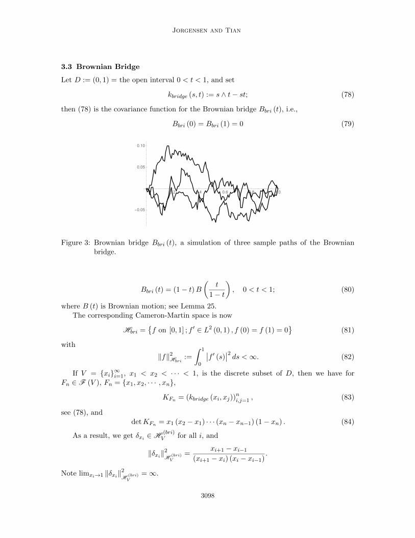
kbridge (s, t) := s ∧ t− st; (78)
then (78) is the covariance function for the Brownian bridge Bbri (t), i.e.,
Bbri (0) = Bbri (1) = 0 (79)
0.2 0.4 0.6 0.8 1.0
-0.05
0.05
0.10
Figure 3: Brownian bridge Bbri (t), a simulation of three sample paths of the Brownianbridge.
Bbri (t) = (1− t)B(
t
1− t
), 0 < t < 1; (80)
where B (t) is Brownian motion; see Lemma 25.The corresponding Cameron-Martin space is now
Hbri =f on [0, 1] ; f ′ ∈ L2 (0, 1) , f (0) = f (1) = 0
(81)
with
‖f‖2Hbri:=
∫ 1
0
∣∣f ′ (s)∣∣2 ds <∞. (82)
If V = xi∞i=1, x1 < x2 < · · · < 1, is the discrete subset of D, then we have forFn ∈ F (V ), Fn = x1, x2, · · · , xn,
KFn = (kbridge (xi, xj))ni,j=1 , (83)
see (78), anddetKFn = x1 (x2 − x1) · · · (xn − xn−1) (1− xn) . (84)
As a result, we get δxi ∈H(bri)V for all i, and
‖δxi‖2
H(bri)V
=xi+1 − xi−1
(xi+1 − xi) (xi − xi−1).
Note limxi→1 ‖δxi‖2
H(bri)V
=∞.
3098
Discrete Reproducing Kernel Hilbert Spaces
3.4 Binomial RKHS
Definition 38 Let V = Z+ ∪ 0; and
kb (x, y) :=
x∧y∑n=0
(x
n
)(y
n
), (x, y) ∈ V × V.
where(xn
)= x(x−1)···(x−n+1)
n! denotes the standard binomial coefficient from the binomialexpansion.
Let H = H (kb) be the corresponding RKHS. Set
en (x) =
(xn
)if n ≤ x
0 if n > x.(85)
Lemma 39 (Alpay and Jorgensen, 2015)
(i) en (·) ∈H , n ∈ V ;
(ii) enn∈V is an orthonormal basis (ONB) in the Hilbert space H .
(iii) Set Fn = 0, 1, 2, . . . , n, and
PFn =n∑k=0
|ek 〉〈 ek| (86)
or equivalently
PFnf =
n∑k=0
〈ek, f〉H ek . (87)
then,
(iv) Formula (87) is well defined for all functions f : V → C, f ∈ Func (V ).
(v) Given f ∈ Func (V ); then
f ∈H ⇐⇒∞∑k=0
|〈ek, f〉H |2 <∞; (88)
and, in this case,
‖f‖2H =∞∑k=0
|〈ek, f〉H |2 .
Fix x1 ∈ V , then we shall apply Lemma 39 to the function f1 = δx1 (in Func (V )),
f1 (y) =
1 if y = x1
0 if y 6= x1.
3099
Jorgensen and Tian
Theorem 2 We have
‖PFn (δx1)‖2H =n∑
k=x1
(k
x1
)2
.
The proof of the theorem will be subdivided in steps; see below.
Lemma 40 (Alpay and Jorgensen, 2015)
(i) For ∀m,n ∈ V , such that m ≤ n, we have
δm,n =
n∑j=m
(−1)m+j
(n
j
)(j
m
). (89)
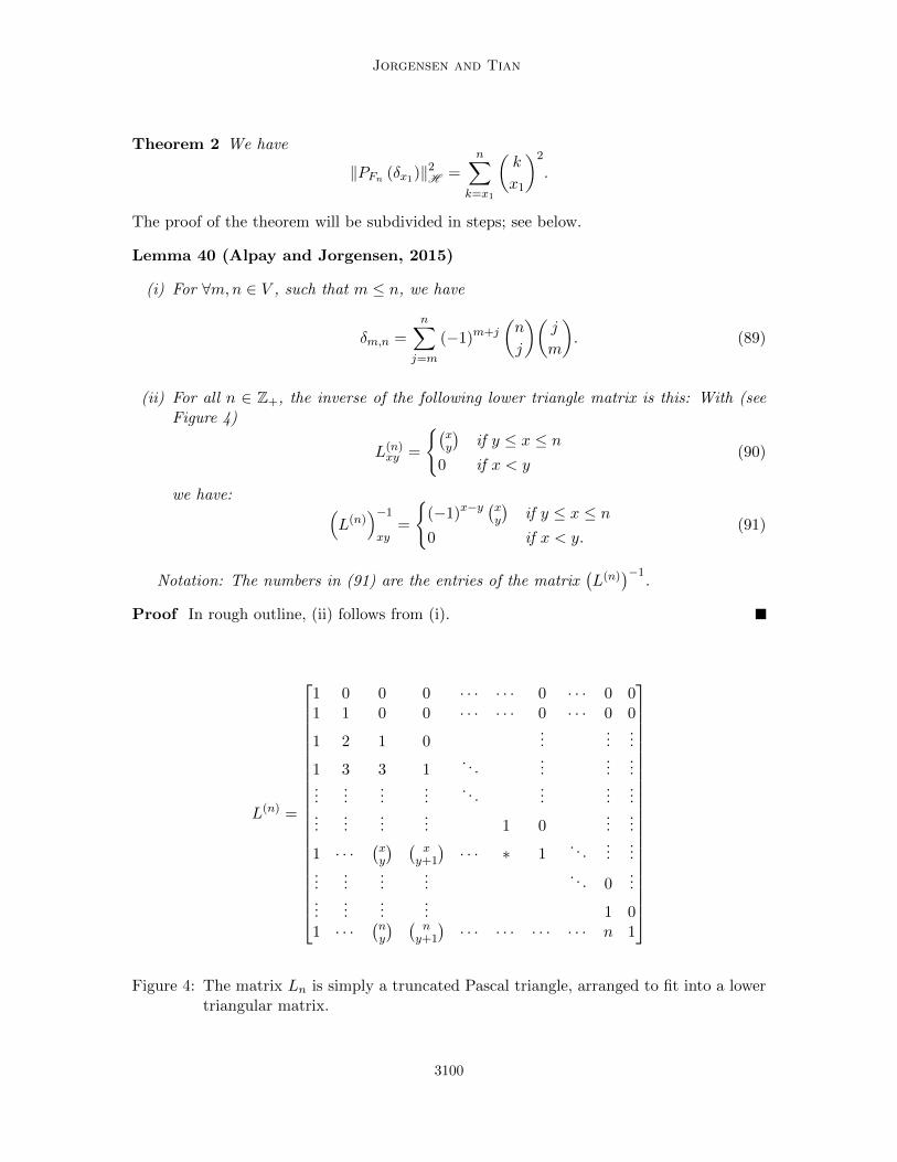
(ii) For all n ∈ Z+, the inverse of the following lower triangle matrix is this: With (seeFigure 4)
L(n)xy =
(xy
)if y ≤ x ≤ n
0 if x < y(90)
we have: (L(n)
)−1
xy=
(−1)x−y
(xy
)if y ≤ x ≤ n
0 if x < y.(91)
Notation: The numbers in (91) are the entries of the matrix(L(n)
)−1.
Proof In rough outline, (ii) follows from (i).
L(n) =
1 0 0 0 · · · · · · 0 · · · 0 01 1 0 0 · · · · · · 0 · · · 0 0
1 2 1 0...
......
1 3 3 1. . .
......
......
......
.... . .
......
......
......
... 1 0...
...
1 · · ·(xy
) (xy+1
)· · · ∗ 1
. . ....
......
......
.... . . 0
......
......
... 1 01 · · ·
(ny
) (ny+1
)· · · · · · · · · · · · n 1
Figure 4: The matrix Ln is simply a truncated Pascal triangle, arranged to fit into a lowertriangular matrix.
3100
Discrete Reproducing Kernel Hilbert Spaces
Corollary 41 Let kb, H , and n ∈ Z+ be as above with the lower triangle matrix Ln. Set
Kn (x, y) = kb (x, y) , (x, y) ∈ Fn × Fn, (92)
i.e., an (n+ 1)× (n+ 1) matrix.
(i) Then Kn is invertible with
K−1n =
(Ltrn)−1
(Ln)−1 ; (93)
an (upper triangle)× (lower triangle) factorization.
(ii) For the diagonal entries in the (n+ 1)× (n+ 1) matrix K−1n , we have:
⟨x,K−1
n x⟩l2
=
n∑k=x
(k
x
)2
Conclusion: Since‖PFn (δx1)‖2H =
⟨x1,K
−1n x1
⟩H
(94)
for all x1 ∈ Fn, we get
‖PFn (δx1)‖2H =n∑
k=x1
(k
x1
)2
= 1 +
(x1 + 1
x1
)2
+
(x1 + 2
x1
)2
+ · · ·+(n
x1
)2
; (95)
and therefore,
‖δx1‖2H =
∞∑k=x1
(k
x1
)2
=∞.
In other words, no δx is in H .
4. Infinite Network of Resistors
Here we introduce a family of positive definite kernels k : V × V → R, defined on infinitesets V of vertices for a given graph G = (V,E) with edges E ⊂ V × V \(diagonal).
There is a large literature dealing with analysis on infinite graphs (Jorgensen and Pearse,2010, 2011, 2013; Okoudjou and Strichartz, 2005; Boyle et al., 2007; Cho and Jorgensen,2011).
Our main purpose here is to point out that every assignment of resistors on the edgesE in G yields a p.d. kernel k, and an associated RKHS H = H (k) such that
δx ∈H , for all x ∈ V . (96)
Definition 42 Let G = (V,E) be as above. Assume
1. (x, y) ∈ E ⇐⇒ (y, x) ∈ E;
3101
Jorgensen and Tian
2. ∃c : E → R+ (a conductance function = 1 / resistance) such that
(i) c(xy) = c(yx), ∀ (xy) ∈ E;
(ii) for all x ∈ V , #y ∈ V | c(xy) > 0
<∞; and
(iii) ∃o ∈ V s.t. for ∀x ∈ V \ o, ∃ edges (xi, xi+1)n−10 ∈ E s.t. xo = 0, and xn = x;
called connectedness.
Given G = (V,E), and a fixed conductance function c : E → R+ as specified above, wenow define a corresponding Laplace operator ∆ = ∆(c) acting on functions on V , i.e., onFunc (V ) by
(∆f) (x) =∑y∼x
cxy (f (x)− f (y)) . (97)
Let H be the Hilbert space defined as follows: A function f on V is in H iff f (o) = 0,and
‖f‖2H :=1
2
∑∑(x,y)∈E⊂V×V
cxy |f (x)− f (y)|2 <∞. (98)
Lemma 43 (Jorgensen and Pearse, 2010) For all x ∈ V \ o, ∃vx ∈H s.t.
f (x)− f (o) = 〈vx, f〉H , ∀f ∈H (99)
where
〈h, f〉H =1
2
∑∑(x,y)∈E
cxy
(h (x)− h (y)
)(f (x)− f (y)) , ∀h, f ∈H . (100)
(The system vx is called a system of dipoles.)
Proof Let x ∈ V \ o, and use (97) together with the Schwarz-inequality to show that
|f (x)− f (o)|2 ≤∑i
1
cxixi+1
∑i
cxixi+1 |f (xi)− f (xi+1)|2 .
An application of Riesz’ lemma then yields the desired conclusion.
Note that vx = v(c)x depends on the choice of base point o ∈ V , and on conductance
function c; see (i)-(ii) and (98).
Now set
k(c) (x, y) = 〈vx, vy〉H , ∀ (xy) ∈ (V \ o)× (V \ o) . (101)
It follows from a theorem that k(c) is a Green’s function for the Laplacian ∆(c) in the sensethat
∆(c)k(c) (x, ·) = δx (102)
where the dot in (102) is the dummy-variable in the action. Note that the solution to (102)is not unique.
3102
Discrete Reproducing Kernel Hilbert Spaces
Lemma 44 (Jorgensen and Pearse, 2011) Let G = (V,E), and conductance functionc : E → R+ be a s specified above; then k(c) in (101) is positive definite, and the cor-responding RKHS H
(k(c))
is the Hilbert space introduced in (98) and (100), called theenergy-Hilbert space.
Proof See Jorgensen et al. (2010; 2011; 2013).
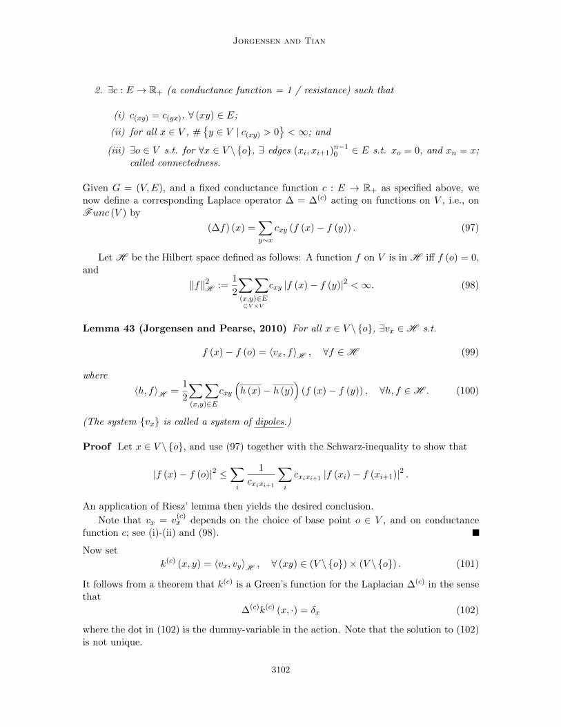
Proposition 45 Let x ∈ V \ o, and let c : E → R+ be specified as above. Let H =H (kc) be the corresponding RKHS. Then δx ∈H , and
‖δx‖2H =∑y∼x
c(xy) =: c (x) . (103)
Proof We study the finite matrices, defined for ∀F ∈ F (V ), by
KF (x, y) = kc (x, y) , (x, y) ∈ F × F. (104)
Fix x ∈ V \ o, and pick F ∈ F (V ) such that
x ∪ y ∈ V | y ∼ x ⊂ F, (105)
see Figure 5; an interior point:
x
y1
FF
Figure 5: Neighborhood of x, see Definition 42 (ii). An interior point x.
Let F ∈ F (V ) be as in (104) and in Figure 5, and let ∆ = ∆(c) be the Laplace operator(97), then for all (x, y) ∈ F × F , we have:⟨
x,K−1F y
⟩l2
= 〈δx,∆δy〉l2= (∆δy) (x)
=
c (x) if y = x; see (103)
−c(xy) if y ∼ x0 for all other values of y
(106)
3103
Jorgensen and Tian
In particular,
supF∈F (V )
(KF δx) (x) <∞;
and in fact,
‖δx‖2H = c (x) , for all x ∈ V \ o,
as claimed in the Proposition.
The last step in the present proof uses the equivalence (i)⇔(ii)⇔(iii) from Theorem 1above.
Finally, we note that the assertion in (106) follows from
∆vx = δx − δo, ∀x ∈ V \ o . (107)
And (107) in turn follows from (99), (97) and a straightforward computation.
Corollary 46 Let G = (V,E) and conductance c : E → R+ be as specified above. Let∆ = ∆(c) be the corresponding Laplace operator. Let H = H (kc) be the RKHS. Then
〈δx, f〉H = (∆f) (x) (108)
and
δx = c (x) vx −∑y∼x
cxyvy (109)
holds for all x ∈ V .
Proof Since the system vx of dipoles in (99) span a dense subspace in H , it is enoughto verify (108) when f = vy for y ∈ V \ o. But in this case, (108) follows from (102) and(106).
Corollary 47 Let G = (V,E), and conductance c : E → R+ be as before; let ∆(c) be
the Laplace operator, and H(c)E the energy-Hilbert space in Definition 42 (Equation (98)).
Let k(c) (x, y) = 〈vx, vy〉HEbe the kernel from (101), i.e., the Green’s function of ∆(c).
Then the two Hilbert spaces HE, and H(k(c))
= RKHS(k(c)), are naturally isometrically
isomorphic via vx 7−→ k(c)x where k
(c)x = k(c) (x, ·) for all x ∈ V .
Proof Let F ∈ F (V ), and let ξ be a function on F ; then∥∥∥∑x∈F
ξ (x) k(c)x
∥∥∥2
H (k(c))=
∑∑F×F
ξ (x)ξ (y) k(c) (x, y)
=(101)
∑∑F×F
ξ (x)ξ (y) 〈vx, vy〉HE
=∥∥∥∑
x∈Fξ (x) vx
∥∥∥2
HE
.
3104
Discrete Reproducing Kernel Hilbert Spaces
The remaining steps in the proof of the Corollary now follows from the standard com-pletion from dense subspaces in the respective two Hilbert spaces HE and H
(k(c)).
In the following we show how the kernels k(c) : V × V → R from (101) in Lemma 43 arerelated to metrics on V ; so called resistance metrics (Jorgensen and Pearse, 2010; Alpayet al., 2013).
Corollary 48 Let G = (V,E), and conductance c : E → R+ be as above; and let k(c) (x, y) :=〈vx, vy〉HE
be the corresponding Green’s function for the graph Laplacian ∆(c).
Then there is a metric R(= R(c) = the resistance metric
), such that
k(c) (x, y) =R(c) (o, x) +R(c) (o, y)−R(c) (x, y)
2(110)
holds on V × V . Here the base-point o ∈ V is chosen and fixed s.t.
〈Vx, f〉HE= f (x)− f (o) , ∀f ∈HE , ∀x ∈ V. (111)
Proof SetR(c) (x, y) = ‖vx − vy‖2HE
. (112)
We proved (Jorgensen and Pearse, 2010) that R(c) (x, y) in (112) indeed defines a metric onV ; the so called resistance metric. It represents the voltage-drop from x to y when 1 Ampis fed into (G, c) at the point x, and then extracted at y.
The verification of (110) is now an easy computation, as follows:
R(c) (o, x) +R(c) (o, y)−R(c) (x, y)
2
=‖vx‖2HE
+ ‖vy‖2HE− ‖vx − vy‖2HE
2= 〈vx, vy〉HE
= k(c) (x, y) by (101).
Proposition 49 In the two cases: (i) B (t), Brownian motion on 0 < t <∞; and (ii) theBrownian bridge Bbri (t), 0 < t < 1, from Section 3 (Figure 3), the corresponding resistancemetric R is as follows:
(i) If V = xi∞i=1 ⊂ (0,∞), x1 < x2 < · · · , then
R(V )B (xi, xj) = |xi − xj | . (113)
(ii) If W = xi∞i=1 ⊂ (0, 1), 0 < x1 < x2 < · · · < 1, then
R(W )bridge (xi, xj) = |xi − xj | · (1− |xi − xj |) . (114)
In the completion w.r.t. the resistance metric R(W )bridge, the two endpoints x = 0 and
x = 1 are identified.
3105
Jorgensen and Tian
4.1 Gaussian Processes
Definition 50 A Gaussian realization of an infinite graph-network G = (V,E), with pre-scribed conductance function c : E → R+, and dipoles (vcx)x∈V \o, is a Gaussian process(Xx)x∈V on a probability space (Ω,F ,P), where Ω is a sample space; F a sigma-algebra ofevents, and P a probability measure s.t., for ∀F ∈ F (V ), the random variables (Xx)x∈F ,are jointly Gaussian with
E (Xx) =
∫ΩXxdP = 0 (115)
and covariance
E (XxXy) = k(c) (x, y) =⟨v(c)x , v(c)
y
⟩HE
; (116)
i.e., the covariance matrix (E (XxXy))(x,y)∈F×F is
KF (x, y) := k(c) (x, y) on F × F. (117)
Lemma 51 (Jorgensen and Pearse, 2010) For all G = (V,E), and c : E → R+, asspecified, Gaussian realizations exist; they are called Gaussian free fields.
Corollary 52 Let G = (V,E), c : E → R+ be as above; and let (Xx)x∈V be an associatedGaussian free field. Then the point Dirac-masses (δx)x∈V have Gaussian realizations
δx = c (x)Xx −∑y∼x
cxyXy, ∀x ∈ V. (118)
Corollary 53 Let G = (V,E), and c : E → R+ be as above. Let Xxx∈V be the corre-sponding Gaussian free field, i.e., with correlation
E (XxXy) = k(c) (x, y) =⟨v(c)x , v(c)
y
⟩HE
(119)
where the dipoles v(c)x ⊂HE are computed w.r.t. a chosen (and fixed) based-point o ∈ V ,
i.e., ⟨v(c)x , f
⟩HE
= f (x)− f (o) , ∀f ∈HE , x ∈ V. (120)
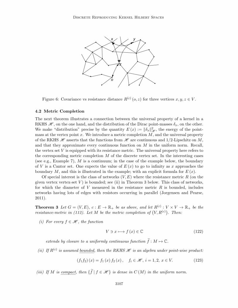
Finally, let R(c) (x, y) be the corresponding resistance metric on V . Then
E (XxXz) + E (XzXy) ≤ E (XxXy) +R(c) (o, z) (121)
holds for all vertices x, y, z ∈ V ; see Figure 6.
Proof Use Corollary 48, and (112). We have
‖vx − vy‖2H ≤ ‖vx − vz‖2H + ‖vz − vy‖2H ,
and (121) now follows from (116).
3106
Discrete Reproducing Kernel Hilbert Spaces
x
z
o
y
Figure 6: Covariance vs resistance distance R(c) (o, z) for three vertices x, y, z ∈ V .
4.2 Metric Completion
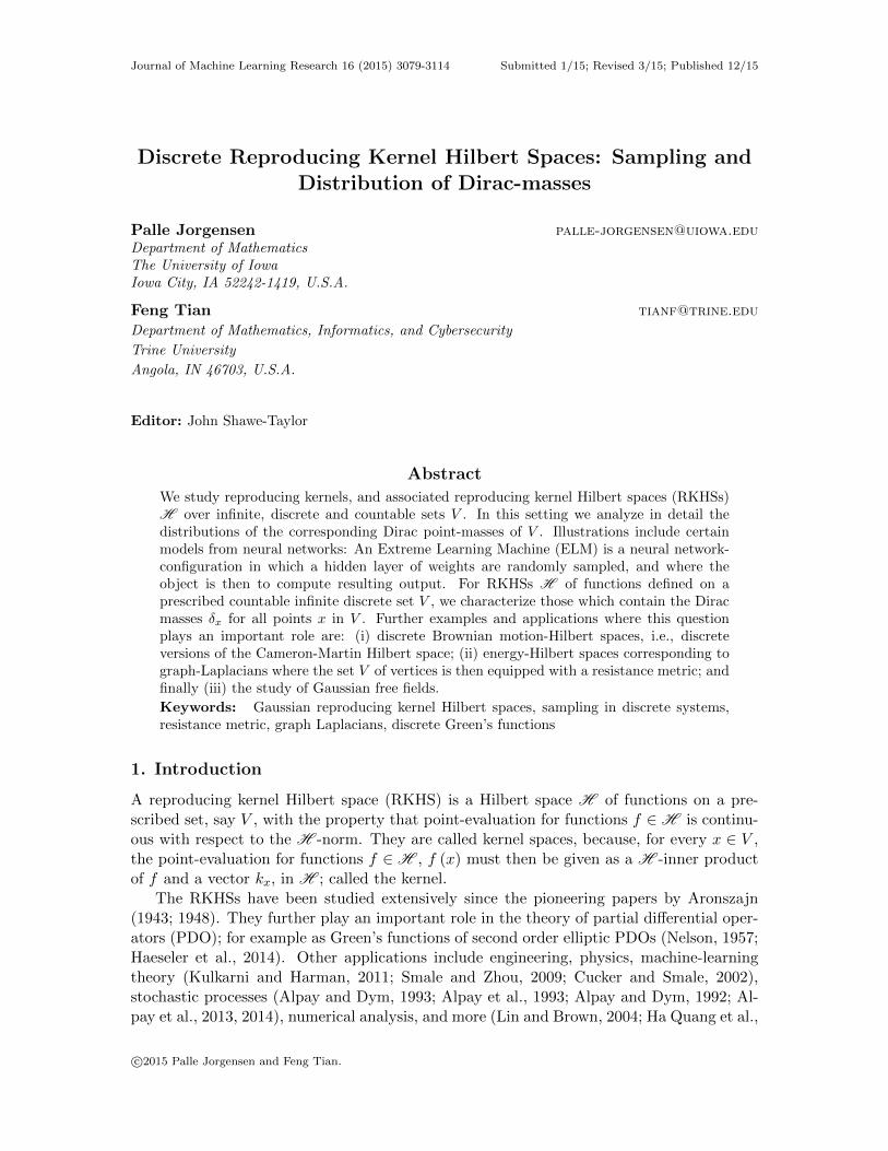
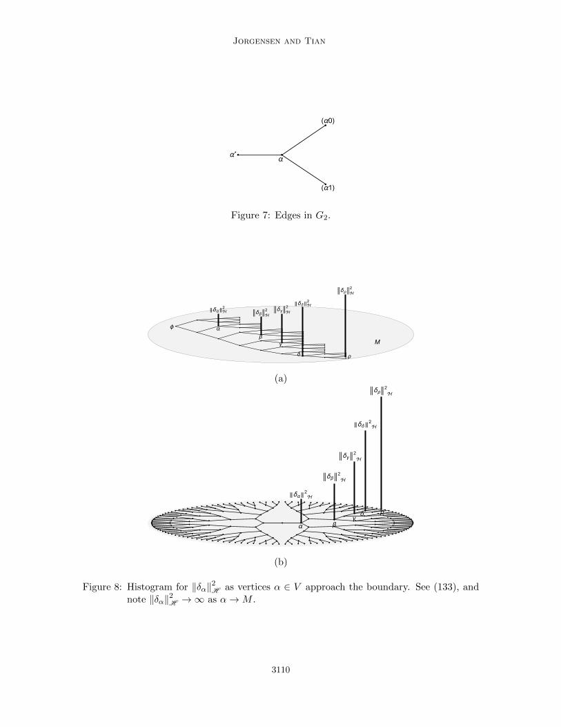
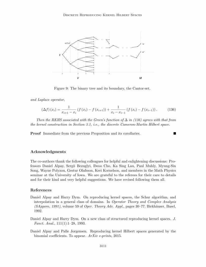
The next theorem illustrates a connection between the universal property of a kernel in aRKHS H , on the one hand, and the distribution of the Dirac point-masses δx, on the other.We make “distribution” precise by the quantity E (x) := ‖δx‖2H , the energy of the point-mass at the vertex point x. We introduce a metric completion M , and the universal propertyof the RKHS H asserts that the functions from H are continuous and 1/2-Lipschitz on M ,and that they approximate every continuous function on M in the uniform norm. Recall,the vertex set V is equipped with its resistance metric. The universal property here refers tothe corresponding metric completion M of the discrete vertex set. In the interesting cases(see e.g., Example 7), M is a continuum; in the case of the example below, the boundaryof V is a Cantor set. One expects the value of E (x) to go to infinity as x approaches theboundary M , and this is illustrated in the example; with an explicit formula for E (x).
Of special interest is the class of networks (V,E) where the resistance metric R (on thegiven vertex vertex-set V ) is bounded; see (ii) in Theorem 3 below. This class of networks,for which the diameter of V measured in the resistance metric R is bounded, includesnetworks having lots of edges with resistors occurring in parallel (Jorgensen and Pearse,2011).
Theorem 3 Let G = (V,E), c : E → R+ be as above, and let R(c) : V × V → R+ be theresistance-metric in (112). Let M be the metric completion of
(V,R(c)
). Then:
(i) For every f ∈H , the function
V 3 x 7−→ f (x) ∈ C (122)
extends by closure to a uniformly continuous function f : M 7→ C.
(ii) If R(c) is assumed bounded, then the RKHS H is an algebra under point-wise product:
(f1f2) (x) = f1 (x) f2 (x) , fi ∈H , i = 1, 2, x ∈ V. (123)
(iii) If M is compact, then f | f ∈H is dense in C (M) in the uniform norm.
3107
Jorgensen and Tian
Proof The assertions in (i) follow from the following two estimates:
Let f ∈H , then
|f (x)− f (y)|2 ≤ ‖f‖2H R(c) (x, y) , ∀x, y ∈ V ; (124)
and
|f (x)| ≤ |f (o)|+R(c) (o, x)12 . (125)
The estimates in (124)-(125), in turn, follow from Corollaries 47 and 48.
To prove (ii), we compute the energy-norm of the product f1 ·f2 where fi ∈H , i = 1, 2;and we use Corollary 47:∑
x
∑y
cxy |f1 (x) f2 (x)− f1 (y) f2 (y)|2
=∑x
∑y
cxy |(f1 (x)− f1 (y)) f2 (x) + f1 (y) (f2 (x)− f2 (y))|2
≤∑x
∑y
cxy
(|f1 (x)− f1 (y)|2 + |f2 (x)− f2 (y)|2
)·(|f2 (x)|2 + |f1 (y)|2
)(by Schwarz inside)
≤(‖f1‖2∞ + ‖f2‖2∞
)·(‖f1‖2H + ‖f2‖2H
);
and we note that the right-side is finite subject to the assumption in (ii).
Proof of (iii): We are assuming here that M is compact, and we shall apply the Stone-Weierstrass theorem to the subalgebra
f∣∣ f ∈H
⊂ C (M) . (126)
Indeed, the conditions for Stone-Weierstrass are satisfied: The functions on LHS in (126)form an algebra, by (ii), closed under complex conjugation; and it separates points in Mby Corollary 48.
Example 7 (The binary tree) Let A = 0, 1, and M :=∏
NA the infinite Cartesianproduct, as a Cantor space. Set V := all finite words:
V =⋃n∈N
(α1, α2, · · · , αn)
∣∣ αi ∈ 0, 1 ; (127)
and set l ((α1, α2, · · · , αn)) =: n.
For ω = (ωk)∞1 ∈M , set
ω∣∣n
:= (ω1, ω2, · · · , ωn) ∈ V. (128)
For two points ω, ω′ ∈M , we shall need the number
l(ω ∩ ω′
)= sup
n : ω
∣∣n
= ω′∣∣n
. (129)
3108
Discrete Reproducing Kernel Hilbert Spaces
Let r : N→ R+ be given such that
r (∅) = 0,∑n∈N
r (n) <∞. (130)
For conductance function c : E → R+, set
cα,(αt) =1
r (l (α)), ∀α ∈ V, t ∈ 0, 1 . (131)
One checks that, when (130) holds, then
limn,m→∞
R(c)(ω∣∣n, ω∣∣m
)= 0.
Consider the graph G2 = (V,E) where the edges are “lines” between α and (αt), wheret ∈ 0, 1. See Figure 7.
Lemma 54 With the settings above, the metric completion R(c) w.r.t. the resistance metricon V is as follows: For ω, ω′ ∈M (see Figure 9),
R(c)(ω, ω′
)= 2
∞∑n=l(ω∩ω′)
r (n) . (132)
Let H be the corresponding energy-Hilbert space ' the RKHS of kc. For α ∈ V , let δα bethe Dirac-mass at the vertex point α. Then
‖δα‖2H =2
r (l (α))+
1
r (l (α)− 1). (133)
(See Figure 8.)
Proof To see this, note that α has the three neighbors sketched in Figure 7, i.e., α∗, (α0),and (α1), where α∗ is the one-truncated word,
R(c)(ω, ω′
)= 2
∞∑n=l(ω∩ω′)
r (n) . (134)
One checks that when (130) is assumed, then the conditions in point (iii) of the theoremare satisfied.
Corollary 55 Now return to the discrete restriction of Brownian motion in Section 3.1.Set V = x1, x2, x3, · · · where the points xi∞i=1 are prescribed such that x1 < x2 < · · · <xi < xi+1 < · · · . We turn V into a weighted graph G as follows: The edges E in G arenearest neighbors; and we define a conductance function c : E → R+ by setting
cxixi+1 :=1
xi+1 − xi, (135)
3109
Jorgensen and Tian
α*
α
(α0)
(α1)
Figure 7: Edges in G2.
ϕ
M
α
β
γ
δ ρ
δαℋ2
δβℋ
2 δγℋ
2δδℋ
2
δρℋ
2
(a)
α βγ
δ ρ
δα2ℋ
δβ2ℋ
δγ2ℋ
δδ2ℋ
δρ2ℋ
(b)
Figure 8: Histogram for ‖δα‖2H as vertices α ∈ V approach the boundary. See (133), andnote ‖δα‖2H →∞ as α→M .
3110
Discrete Reproducing Kernel Hilbert Spaces
ϕ
V M
ω⋂ω ' ω
ω '
0 2 3 4 n
Figure 9: The binary tree and its boundary, the Cantor-set.
and Laplace operator,
(∆f) (xi) =1
xi+1 − xi(f (xi)− f (xi+1)) +
1
xi − xi−1(f (xi)− f (xi−1)) . (136)
Then the RKHS associated with the Green’s function of ∆ in (136) agrees with that fromthe kernel construction in Section 3.1, i.e., the discrete Cameron-Martin Hilbert space.
Proof Immediate from the previous Proposition and its corollaries.
Acknowledgments
The co-authors thank the following colleagues for helpful and enlightening discussions: Pro-fessors Daniel Alpay, Sergii Bezuglyi, Ilwoo Cho, Ka Sing Lau, Paul Muhly, Myung-SinSong, Wayne Polyzou, Gestur Olafsson, Keri Kornelson, and members in the Math Physicsseminar at the University of Iowa. We are grateful to the referees for their care to detailsand for their kind and very helpful suggestions. We have revised following them all.
References
Daniel Alpay and Harry Dym. On reproducing kernel spaces, the Schur algorithm, andinterpolation in a general class of domains. In Operator Theory and Complex Analysis(SApporo, 1991), volume 59 of Oper. Theory Adv. Appl., pages 30–77. Birkhauser, Basel,1992.
Daniel Alpay and Harry Dym. On a new class of structured reproducing kernel spaces. J.Funct. Anal., 111(1):1–28, 1993.
Daniel Alpay and Palle Jorgensen. Reproducing kernel Hilbert spaces generated by thebinomial coefficients. To appear. ArXiv e-prints, 2015.
3111
Jorgensen and Tian
Daniel Alpay, Vladimir Bolotnikov, Aad Dijksma, and Henk de Snoo. On some operatorcolligations and associated reproducing kernel Hilbert spaces. In Operator Extensions,Interpolation of Functions and Related Topics, volume 61 of Oper. Theory Adv. Appl.,pages 1–27. Birkhauser, Basel, 1993.
Daniel Alpay, Palle Jorgensen, Ron Seager, and Dan Volok. On discrete analytic functions:products, rational functions and reproducing kernels. J. Appl. Math. Comput., 41(1-2):393–426, 2013.
Daniel Alpay, Palle Jorgensen, and Dan Volok. Relative reproducing kernel Hilbert spaces.Proc. Amer. Math. Soc., 142(11):3889–3895, 2014.
Nachman Aronszajn. La theorie des noyaux reproduisants et ses applications. I. Proc.Cambridge Philos. Soc., 39:133–153, 1943.
Nachman Aronszajn. Reproducing and pseudo-reproducing kernels and their application tothe partial differential equations of physics. Studies in partial differential equations. Tech-nical report 5, preliminary note. Harvard University, Graduate School of Engineering.,1948.
Brighid Boyle, Kristin Cekala, David Ferrone, Neil Rifkin, and Alexander Teplyaev. Elec-trical resistance of N -gasket fractal networks. Pacific J. Math., 233(1):15–40, 2007.
Ola Bratteli and Palle Jorgensen. Wavelets Through a Looking Glass. Applied and Numer-ical Harmonic Analysis. Birkhauser Boston, Inc., Boston, MA, 2002.
Andrea Caponnetto, Charles A. Micchelli, Massimiliano Pontil, and Yiming Ying. Universalmulti-task kernels. J. Mach. Learn. Res., 9:1615–1646, 2008.
Ilwoo Cho and Palle Jorgensen. Free probability induced by electric resistance networks onenergy Hilbert spaces. Opuscula Math., 31(4):549–598, 2011.
Felipe Cucker and Steve Smale. On the mathematical foundations of learning. Bull. Amer.Math. Soc. (N.S.), 39(1):1–49, 2002.
Minh Ha Quang, Sung Ha Kang, and Triet M. Le. Image and video colorization usingvector-valued reproducing kernel Hilbert spaces. J. Math. Imaging Vision, 37(1):49–65,2010.
S. Haeseler, M. Keller, D. Lenz, J. Masamune, and M. Schmidt. Global properties ofDirichlet forms in terms of Green’s formula. ArXiv e-prints, 2014.
Haakan Hedenmalm and Pekka J. Nieminen. The Gaussian free field and Hadamard’svariational formula. Probab. Theory Related Fields, 159(1-2):61–73, 2014.
Palle Jorgensen and Erin P.J. Pearse. A Hilbert space approach to effective resistancemetric. Complex Anal. Oper. Theory, 4(4):975–1013, 2010.
Palle Jorgensen and Erin P.J. Pearse. Resistance boundaries of infinite networks. InRandom walks, boundaries and spectra, volume 64 of Progr. Probab., pages 111–142.Birkhauser/Springer Basel AG, Basel, 2011.
3112
Discrete Reproducing Kernel Hilbert Spaces
Palle Jorgensen and Erin P.J. Pearse. A discrete Gauss-Green identity for unboundedLaplace operators, and the transience of random walks. Israel J. Math., 196(1):113–160,2013.
Samuel Karlin and Zvi Ziegler. Some inequalities of total positivity in pure and appliedmathematics. In Total positivity and its applications (Jaca, 1994), volume 359 of Math.Appl., pages 247–261. Kluwer Acad. Publ., Dordrecht, 1996.
Sanjeev Kulkarni and Gilbert Harman. An elementary introduction to statistical learningtheory. Wiley Series in Probability and Statistics. John Wiley & Sons, Inc., Hoboken,NJ, 2011.
Sneh Lata and Vern Paulsen. The Feichtinger conjecture and reproducing kernel Hilbertspaces. Indiana Univ. Math. J., 60(4):1303–1317, 2011.
Yi Lin and Lawrence D. Brown. Statistical properties of the method of regularization withperiodic Gaussian reproducing kernel. Ann. Statist., 32(4):1723–1743, 2004.
Edward Nelson. Kernel functions and eigenfunction expansions. Duke Math. J., 25:15–27,1957.
Kasso A. Okoudjou and Robert S. Strichartz. Weak uncertainty principles on fractals. J.Fourier Anal. Appl., 11(3):315–331, 2005.
Kasso A. Okoudjou, Robert S. Strichartz, and Elizabeth K. Tuley. Orthogonal polynomialson the Sierpinski gasket. Constr. Approx., 37(3):311–340, 2013.
Carl Edward Rasmussen and Christopher K. I. Williams. Gaussian processes for machinelearning. Adaptive Computation and Machine Learning. MIT Press, Cambridge, MA,2006.
Bernhard Schlkopf and Alexander J. Smola. Learning with Kernels: Support Vector Ma-chines, Regularization, Optimization, and Beyond (Adaptive Computation and MachineLearning). The MIT Press, 1st edition, 12 2001.
Oded Schramm and Scott Sheffield. A contour line of the continuum Gaussian free field.Probab. Theory Related Fields, 157(1-2):47–80, 2013.
John Shawe-Taylor and Nello Cristianini. Kernel Methods for Pattern Analysis. CambridgeUniversity Press, 2004.
Steve Smale and Ding-Xuan Zhou. Online learning with Markov sampling. Anal. Appl.(Singap.), 7(1):87–113, 2009.
Ingo Steinwart. On the influence of the kernel on the consistency of support vector machines.J. Mach. Learn. Res., 2:67–93, March 2002.
Robert S. Strichartz. Transformation of spectra of graph Laplacians. Rocky Mountain J.Math., 40(6):2037–2062, 2010.
3113
Jorgensen and Tian
Robert S. Strichartz and Alexander Teplyaev. Spectral analysis on infinite Sierpinskifractafolds. J. Anal. Math., 116:255–297, 2012.
Mirjana Vuletic. The Gaussian free field and strict plane partitions. In 25th InternationalConference on Formal Power Series and Algebraic Combinatorics (FPSAC 2013), Dis-crete Math. Theor. Comput. Sci. Proc., AS, pages 1041–1052. Assoc. Discrete Math.Theor. Comput. Sci., Nancy, 2013.
Haizhang Zhang, Yuesheng Xu, and Qinghui Zhang. Refinement of operator-valued repro-ducing kernels. J. Mach. Learn. Res., 13:91–136, 2012.
3114