1

Chapter 4

Discrete Probability Distributions

2

Random Variables

The outcome of an experiment need not be a number, for example, the outcome when a coin is tossed can be 'heads' or 'tails'. However, we often want to represent outcomes as numbers. A random variable is a function that associates a unique numerical value with every outcome of an experiment. The value of the random variable will vary from trial to trial as the experiment is repeated.

A real valued function defined on the sample space S is denoted by an upper case roman letter, X, Y... and is called a random variable.

Definition-Random Variable

A random variable has either an associated probability distribution (discrete random variable) or probability density function (continuous random variable).

A numeric function that assigns probabilities to different events in a sample space.

3

Basic Concept

Many random variables associated with statistical experiments have similar properties and can be described by essentially the same probability distribution. However, the distribution of a random variable X depends on how the data were produced. Therefore, we should choose the probability distribution that correctly describes theobservations and variables being generated by an experiment.

Probability distribution may be either discrete or continuous, depending on the characteristics of the random variable to which it applies.

Many random variables associated with statistical experiments have similar properties and can be described by essentially the same probability distribution. However, the distribution of a random variable X depends on how the data were produced. Therefore, we should choose the probability distribution that correctly describes theobservations and variables being generated by an experiment.

Probability distribution may be either discrete or continuous, depending on the characteristics of the random variable to which it applies.

4

Discrete random variable

Continuous random variable

A random variable for which there exists a discrete set of values with specified probabilities is a discrete random variable.

Continuous data is information that can be measured on a continuum or scale.

Discrete data is information that can be categorized into a classification.

A random variable whose possible values cannot be enumerated is a continuous random variable.

5

Suppose a coin is tossed 2 times. Let us consider the random variable associated with the number of heads.

HH

HT

TH

TT

0

1

2

1/4

2/4

X

Discrete random variable

Probability-massfunction

sample space real value probability

Probability-mass function of random variable of X

6

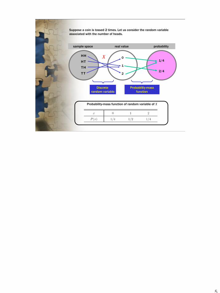
{ , , , },1( ) ( ) ( ) ( )4

S HH HT TH TT

P HH P HT P TH P TT

=

= = = =

7

Karl Pearson is best known for the statistic that bears his name the "Pearson Product-Moment Correlation Coefficient".

Karl Pearson (1857-1936)

The Probability-Mass Function for a Discrete Random Variable

Pearson's revolutionary idea, we do not look upon experimental results as carefully measured numbers in their own right. Instead, they are examples of a scatter of numbers, a distribution of numbers, to use the more accepted term.

This distribution of numbers can be written as a mathematical formula that tells us the probability that an observed number will be a given value.

8

Probability distributionfor discrete random variable

for continuous random variable

The number actually takes in a specific experiment is unpredictable. We can only talk about probabilities of the values and not aboutcertainty of the values. The results of individual experiments are random because they are unpredictable. The statistical models of distributions enable us to describe the mathematical nature of that randomness.

The four parameters that completely describe a member of the Pearson System are called

1. mean - the central value about which the measurements scatter, 2. standard deviation - how far most of the measurements scatter

about the mean, 3. symmetry - the degree to which the measurements pile up on only

one side of the mean, 4. kurtosis - how far rare measurements scatter from the mean.

9

The probability-mass function (probability distribution) is a mathematical relationship that gives the probability of observing each value of x of a discrete random variable X. We shall denote the probability of x by the symbol P(X = x).

Definition

The Probability-Mass Functions for a Discrete Random Variable

Thus, the probability distribution for a discrete random variable x may be given :

x

( )P x 1p

1x 2x nxL

np2p L

where is the probability that the variable x assume the value

( 1, 2, ).kx k n= L

kp

10

{ , , , }, ( )S HH HT TH TT P H p= =

Properties of the probability distribution for a discrete random variable x

1. 0 ( ) 12. ( ) 1

all x

P xP x

≤ ≤

=∑

Suppose you were to toss two coins over and over again a very large number of times and record the number x of heads for each toss. A relative frequency distribution for the resulting collection of 0’s, 1’s and 2’s would be very similar to the probability distribution. In fact, if it were possible to repeat the experiment an infinitely large number of times, the two distributions would be almost identical.

Relationship between the probability distribution for a discreterandom variable and the relative frequency distribution of data:

11

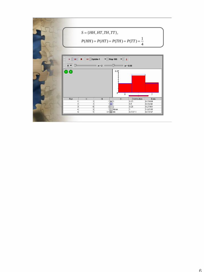
Probability-Mass Function and Cumulative Distribution Function

Probability function for discrete random variable is referred to as probability mass functions.

The probability mass function (PMF) for a discrete random variable X is

( ) ( )XP x P X x= =

The cumulative distribution function (CDF) for a random variable X is

( ) ( )XF x P X x= ≤

0.25

0.5

0.75

1.0

0.25

0.5

0.75

1.0

PMF CDF

0 1 2 0 1 2

12

The Expected Value of a Discrete Random Variable

The expected value is the probability-weighted average of the possible outcomes of a random variable. The mathematical representation for a expected value of a discrete random variable X is

The expected value of a random variable X, denoted by the same symbol of the mean of the population , is equal to the mean of the random variable and can be calculated by multiplying all possible values of X by their probabilities and adding the results.

μ

∑=

===R

iii xXPxXE

1)()(μ

We’d like to determine the average value for a discrete random variable that results from multiple experiments. This average value called the expected value.

13

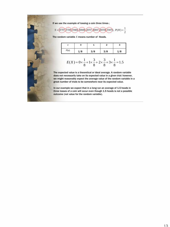
If we use the example of tossing a coin three times ;

1{ , , , , , , , }, ( )2

S TTT TTH THH HHH HTT HHT HTH THT P H= =

x 0 1 2 3

P(x)

The random variable X means number of Heads.

The expected value is a theoretical or ideal average. A random variable does not necessarily take on its expected value in a given trial: however, we might reasonably expect the average value of the random variable in a great number of trials to be somewhere near its expected value.

In our example we expect that in a long run an average of 1.5 heads in three tosses of a coin will occur even though 1.5 heads is not a possible outcome (not value for the random variable).

1/8 3/8 3/8 1/8

5.1813

832

831

810)( =×+×+×+×=XE

14

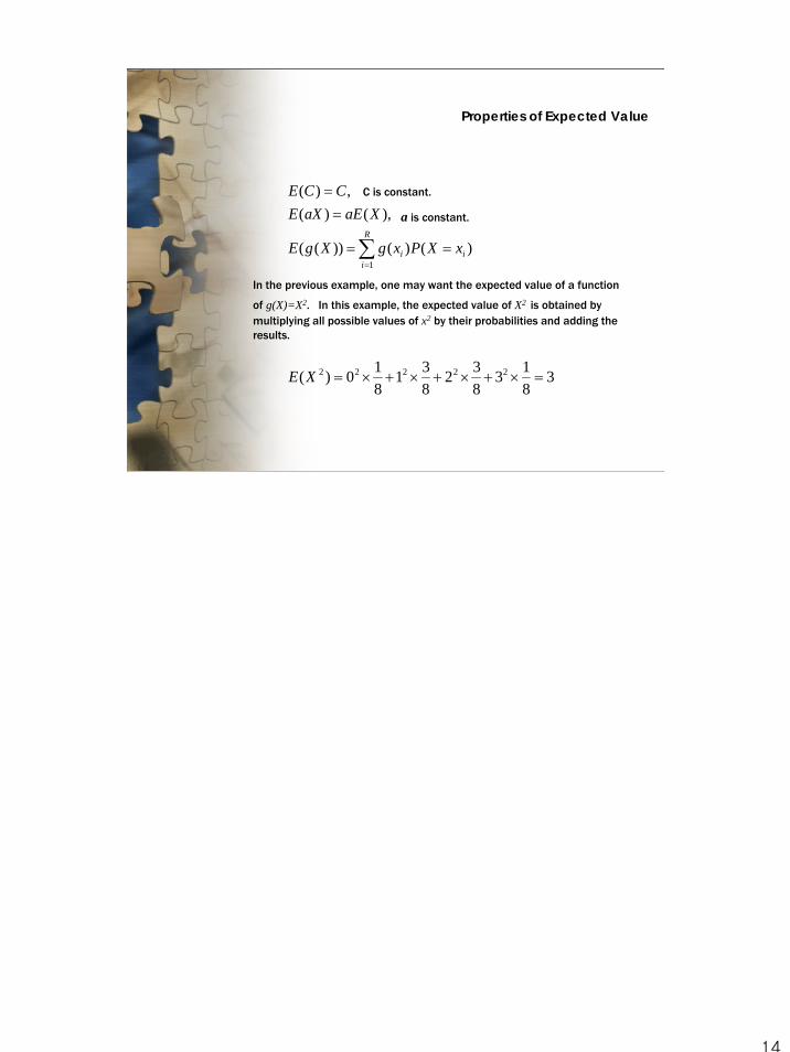
In the previous example, one may want the expected value of a function

of g(X)=X2. In this example, the expected value of X2 is obtained by multiplying all possible values of x2 by their probabilities and adding the results.

Properties of Expected Value

∑=

==

==

R

iii xXPxgXgE

XaEaXECCE

1)()())((

),()(,)( C is constant.

a is constant.

3813

832

831

810)( 22222 =×+×+×+×=XE

15

Suppose a new drug for high blood pressure is introduced, and a physician agrees to use it on a trial basis on the first 4 untreated hypertensives. Form previous experience, the probability that 0 patients out of 4 will be brought under control is .008, 1 patient out of 4 is .076, 2 patients out of 4 is .265, 3 patients out of 4 is .411, and all 4 patients is .240.

What is the expected value for number of patients brought under control with a new drug?

Example

Expected Value Computation

Event Probability X

0 patient out of 4 .008 0 0

1 patient out of 4 .076 1 .076

2 patients out of 4 .265 2 .530

3 patients out of 4 .411 3 1.233

All 4 patients .240 4 .960

( )i ix P X x=

799.2960.233.1530.076.0)( =++++=XE

16

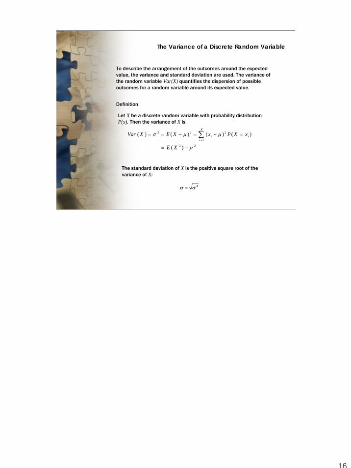
The Variance of a Discrete Random Variable

∑=

=−=−==R

iii xXPxXEXVar

1

222 )()()()( μμσ

To describe the arrangement of the outcomes around the expected value, the variance and standard deviation are used. The variance of the random variable Var(X) quantifies the dispersion of possible outcomes for a random variable around its expected value.

Definition

Let X be a discrete random variable with probability distribution P(x). Then the variance of X is

The standard deviation of X is the positive square root of the variance of X:

2σ σ=

22 )( μ−= XE

17

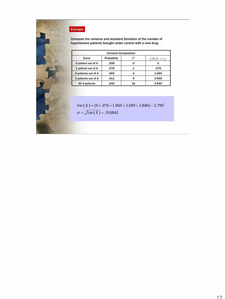
Example

Compute the variance and standard deviation of the number of hypertensive patients brought under control with a new drug.

Variance Computation

Event Probability X2

0 patient out of 4 .008 0 0

1 patient out of 4 .076 1 .076

2 patients out of 4 .265 4 1.060

3 patients out of 4 .411 9 3.699

All 4 patients .240 16 3.840

)(2ii xXPx =

916842.)(

799.2)840.3699.3060.1076.0()( 2

==

−++++=

XVar

XVar

σ

18

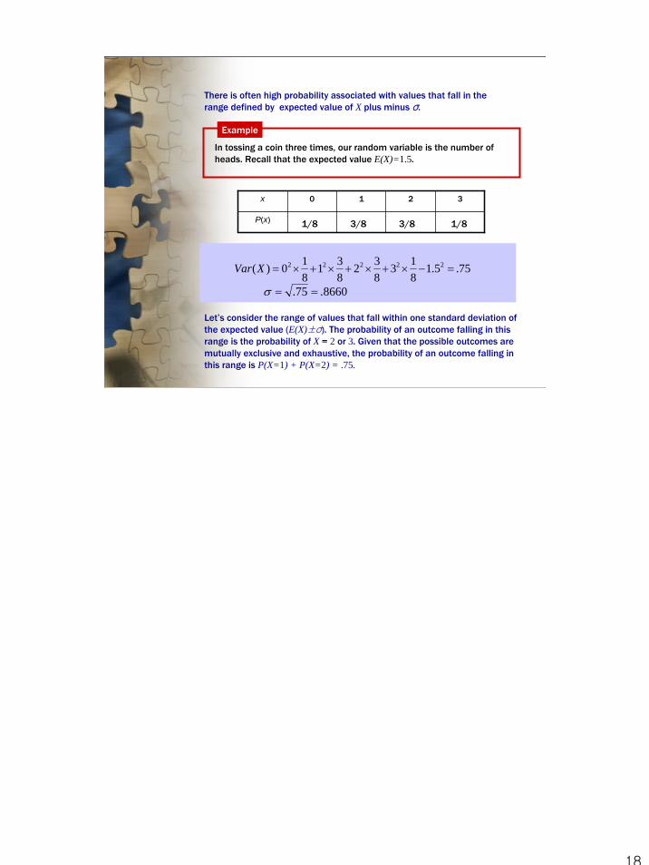
There is often high probability associated with values that fall in the range defined by expected value of X plus minus σ.

In tossing a coin three times, our random variable is the number of heads. Recall that the expected value E(X)=1.5.

Example

75.5.1813

832

831

810)( 22222 =−×+×+×+×=XVar

x 0 1 2 3

P(x) 1/8 3/8 3/8 1/8

8660.75. ==σ

Let’s consider the range of values that fall within one standard deviation of the expected value (E(X)±σ). The probability of an outcome falling in this range is the probability of X = 2 or 3. Given that the possible outcomes are mutually exclusive and exhaustive, the probability of an outcome falling in this range is P(X=1) + P(X=2) = .75.

19

Permutations and Combinations

In probability analysis, it often necessary to determine the number of different outcomes that can occur. There are principles and shortcuts in making these determinations. It is important to understand these principles because without them, the total number of outcomes may be difficult to determine.

In probability analysis, it often necessary to determine the number of different outcomes that can occur. There are principles and shortcuts in making these determinations. It is important to understand these principles because without them, the total number of outcomes may be difficult to determine.

Multiplication Rule of Counting

The multiple rules of counting applies when there is a series of k decisions to make, where each decision, i, can be made in ways. That is, the first decision can be made in ways, the second decision, given in the first, can be made in ways, and so on through the kthdecision.

in1n

2n

Counting Principle

20

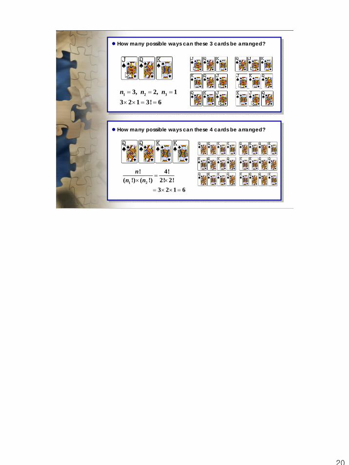
How many possible ways can these 3 cards be arranged?

1 2 33, 2, 13 2 1 3! 6n n n= = =

× × = =

How many possible ways can these 4 cards be arranged?

1 2

! 4!( !) ( !) 2! 2!

3 2 1 6

nn n

=× ×

= × × =

21

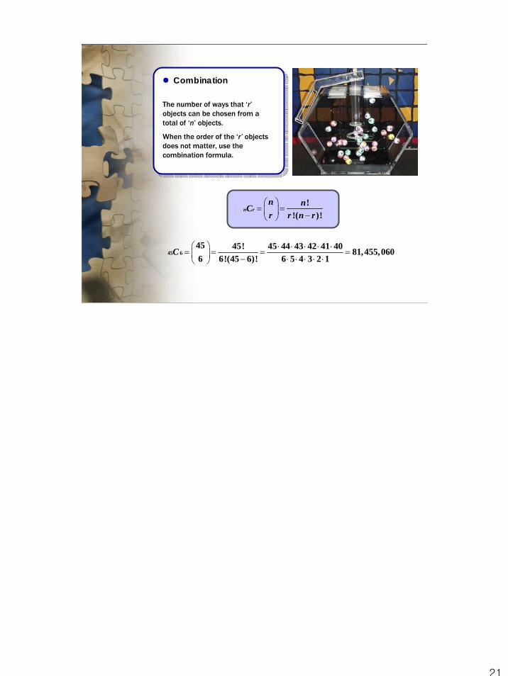
The number of ways that ‘r’objects can be chosen from a total of ‘n’ objects.

When the order of the ‘r’ objects does not matter, use the combination formula.

Combination

!!( )!

n rn nCr r n r

⎛ ⎞= =⎜ ⎟ −⎝ ⎠

45 645 45! 45 44 43 42 41 40 81,455,0606 6!(45 6)! 6 5 4 3 2 1

C⎛ ⎞ ⋅ ⋅ ⋅ ⋅ ⋅

= = = =⎜ ⎟ − ⋅ ⋅ ⋅ ⋅ ⋅⎝ ⎠

22

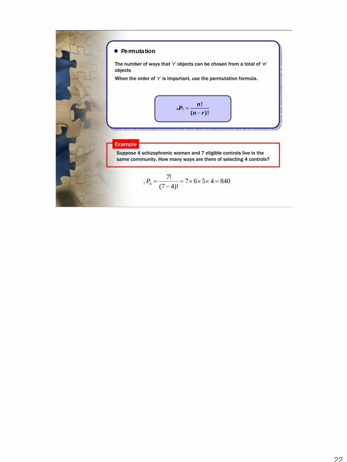
Permutation

The number of ways that ‘r’ objects can be chosen from a total of ‘n’objects

When the order of ‘r’ is important, use the permutation formula.

!( )!

n rnP

n r=

−

Suppose 4 schizophrenic women and 7 eligible controls live in the same community. How many ways are there of selecting 4 controls?

Example

8404567)!47(

!747 =×××=

−=P

23

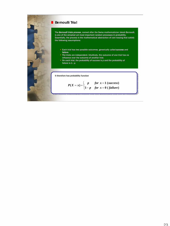
Bernoulli Trial

The Bernoulli trials process, named after the Swiss mathematician Jakob Bernoulli, is one of the simplest yet most important random processes in probability. Essentially, the process is the mathematical abstraction of coin tossing that satisfy the following assumptions:

The Bernoulli trials process, named after the Swiss mathematician Jakob Bernoulli, is one of the simplest yet most important random processes in probability. Essentially, the process is the mathematical abstraction of coin tossing that satisfy the following assumptions:

Each trial has two possible outcomes, generically called success and failure. The trials are independent. Intuitively, the outcome of one trial has no influence over the outcome of another trial. On each trial, the probability of success is p and the probability of failure is 1 - p.

Each trial has two possible outcomes, generically called success and failure. The trials are independent. Intuitively, the outcome of one trial has no influence over the outcome of another trial. On each trial, the probability of success is p and the probability of failure is 1 - p.

It therefore has probability function

1 ( )( )

1 0 ( )p for x success

P X xp for x failure

=⎧= = ⎨ − =⎩

24

which can also be written

1( ) (1 )x xP X x p p −= = −

P(x) for p=0.6

x

( )( )

22 2

2 2 2

2

( ) 1 0 (1 )

( ) ( ( )) ( ) ( )

1 0 (1 )

(1 )

E X p p p

Var X E X E X E X E X

p p p

p p p p

= ⋅ + ⋅ − =

= − = −

= ⋅ + ⋅ − −

= − = −

The Bernoulli trials process is characterized by a single parameter p.

25

Binomial Distribution

One of the most frequently encountered discrete distribution in many disciplines, is the binomial distribution. The binomial distribution utilizes the counting rules and the multiplication rule.

A binomial random variable is the number of successes that will occur in ‘n’Bernoulli trials assuming

One of the most frequently encountered discrete distribution in many disciplines, is the binomial distribution. The binomial distribution utilizes the counting rules and the multiplication rule.

A binomial random variable is the number of successes that will occur in ‘n’Bernoulli trials assuming

The probability of a success (p) or failure (1-p) remains constant from trial to trial.The trials are independent.

The probability of a success (p) or failure (1-p) remains constant from trial to trial.The trials are independent.

The number of such ‘success’ can range anywhere from 0 to n.

If the outcome of each Bernoulli trial (Xk) is random, the total number of successes in ‘n’ trials ( ) will also be random. ∑

=

=n

kiXY

1

26

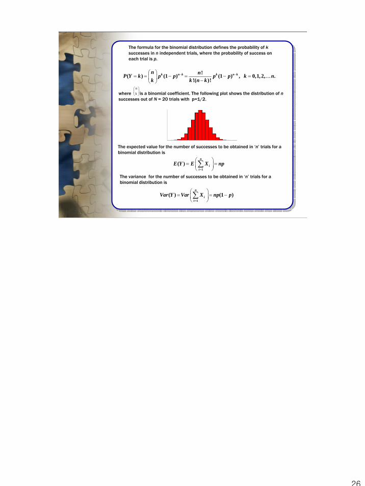
!( ) (1 ) (1 ) , 0,1, 2, .!( )!

k n k k n kn nP Y k p p p p k nk k n k

− −⎛ ⎞= = − = − =⎜ ⎟ −⎝ ⎠

K

where is a binomial coefficient. The following plot shows the distribution of nsuccesses out of N = 20 trials with p=1/2.

nk⎛ ⎞⎜ ⎟⎝ ⎠

The expected value for the number of successes to be obtained in ‘n’ trials for a binomial distribution is

The variance for the number of successes to be obtained in ‘n’ trials for a binomial distribution is

1( )

n

ii

E Y E X np=

⎛ ⎞= =⎜ ⎟

⎝ ⎠∑

1

( ) (1 )n

ii

Var Y Var X np p=

⎛ ⎞= = −⎜ ⎟

⎝ ⎠∑

The formula for the binomial distribution defines the probability of ksuccesses in n independent trials, where the probability of success on each trial is p.

27

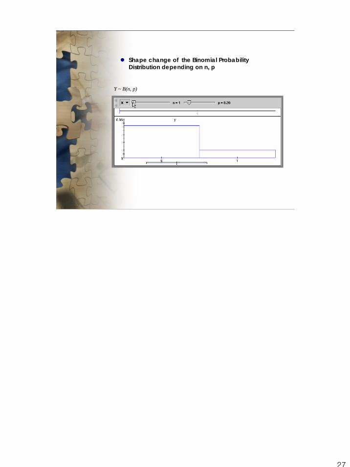
Shape change of the Binomial Probability Distribution depending on n, p

Y

Y ~ B(n, p)

28

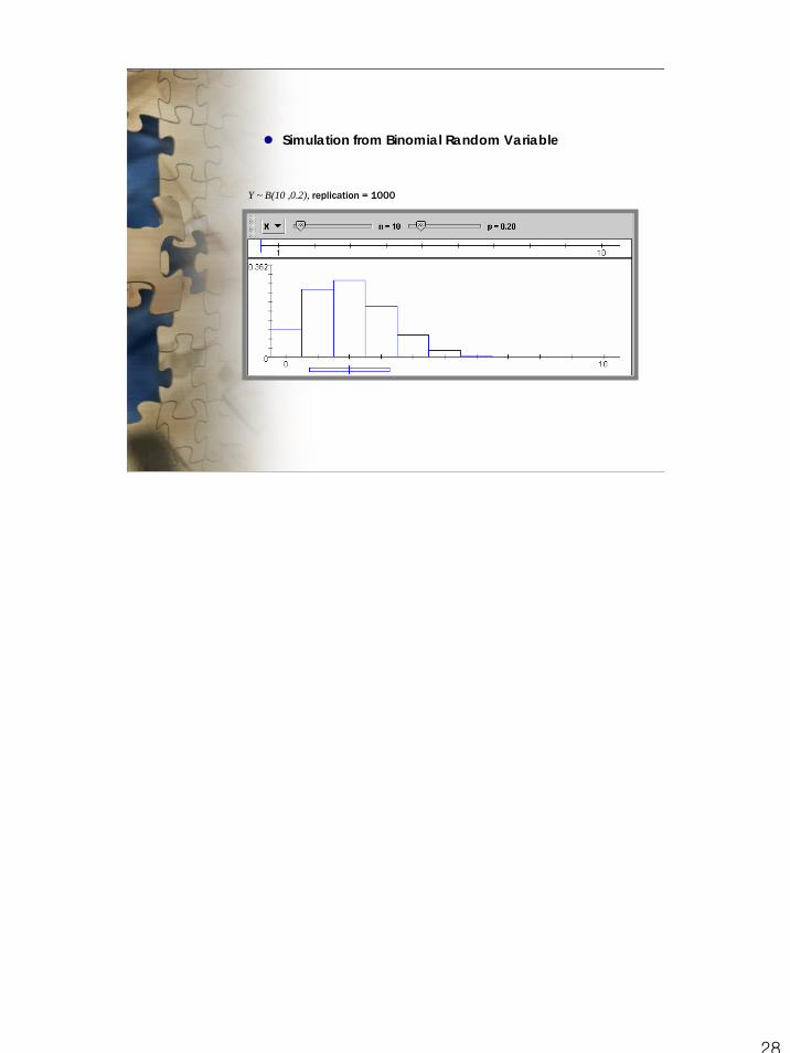
Y ~ B(10 ,0.2), replication = 1000

Simulation from Binomial Random Variable

29

Any one cell has 75% chance of being a neutrophil.

1. Construct the probability distribution for the number of neutrophils out of 4 cells.

0 4 0

1 4 1

2 4 2

3 4 3

4

4!( 0) (0.75) (1 0.75) 0.00391.0!(4 0)!

4!( 1) (0.75) (1 0.75) 0.04687.1!(4 1)!

4!( 2) (0.75) (1 0.75) 0.21094.2!(4 2)!

4!( 3) (0.75) (1 0.75) 0.42187.3!(4 3)!

4!( 4) (0.75)4!(4 4)!

P Y

P Y

P Y

P Y

P Y

−

−

−

−

= = − =−

= = − =−

= = − =−

= = − =−

= =−

4 4(1 0.75) 0.31641.−− =

Out of 4 cells, the number of neutrophils could be 0, 1, 2, 3, or 4 cells.

The binomial probability distribution is determined by computing the probability of each of these collectively exhaustive events.

Example

30

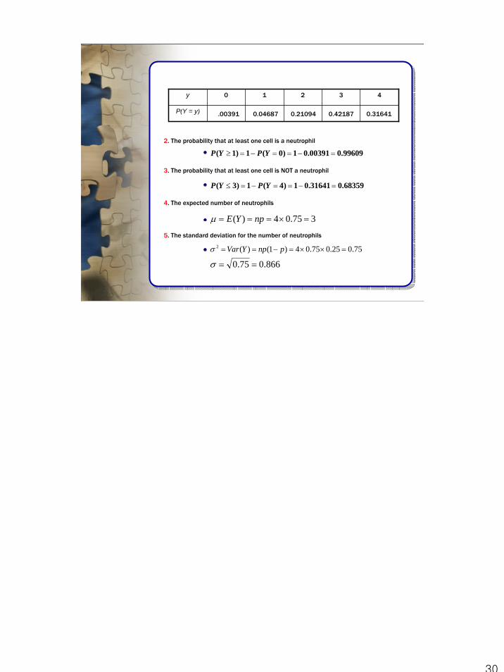
2. The probability that at least one cell is a neutrophil

( 1) 1 ( 0) 1 0.00391 0.99609P Y P Y≥ = − = = − =

3. The probability that at least one cell is NOT a neutrophil

( 3) 1 ( 4) 1 0.31641 0.68359P Y P Y≤ = − = = − =

4. The expected number of neutrophils

5. The standard deviation for the number of neutrophils

y 0 1 2 3 4

P(Y = y) .00391 0.04687 0.21094 0.42187 0.31641

375.04)( =×=== npYEμ

75.025.075.04)1()(2 =××=−== pnpYVarσ

866.075.0 ==σ

31

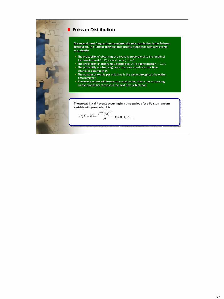
Poisson Distribution

The second most frequently encountered discrete distribution is the Poisson distribution. The Poisson distribution is usually associated with rare events (e.g., death).

The second most frequently encountered discrete distribution is the Poisson distribution. The Poisson distribution is usually associated with rare events (e.g., death).

The probability of observing one event is proportional to the length of the time interval Δt: P(an event occurs) ≈ λΔtThe probability of observing 0 events over Δt is approximately 1– λΔt.The probability of observing more than one event over this time interval is essentially 0.The number of events per unit time is the same throughout the entire time interval t.If an event occurs within one time subinterval, then it has no bearing on the probability of event in the next time subinterval.

The probability of observing one event is proportional to the length of the time interval Δt: P(an event occurs) ≈ λΔtThe probability of observing 0 events over Δt is approximately 1– λΔt.The probability of observing more than one event over this time interval is essentially 0.The number of events per unit time is the same throughout the entire time interval t.If an event occurs within one time subinterval, then it has no bearing on the probability of event in the next time subinterval.

The probability of k events occurring in a time period t for a Poisson random variable with parameter λ is

!)()(

ktekXP

kt λλ−

== , k = 0, 1, 2, …

32

The expected value for the number of events occurring in a time period t is

tXE λμ ==)(

The variance for the number of events occurring in a time period t is

tXVar λμ ==)(

Example

Suppose the number of deaths from typhoid fever over 1-year period is Poisson distributed with parameter μ = 4.6. What is the probability that we have more than 2 deaths over a six month period?

Because μ = λt = 4.6 with t = 1 year, it follows that λ = 4.6. For a 6-month period μ1 = λt1 = 2.3 with t1 = 0.5. Let X be the number of deaths in 6 months.

)2()1()0(1)2(

265.0!2

)3.2()2(

231.0!1

)3.2()1(

100.0)0(

23.2

13.2

3.2

=−=−=−=>

===

===

===

−

−

−

XPXPXPXP

eXP

eXP

eXP

33

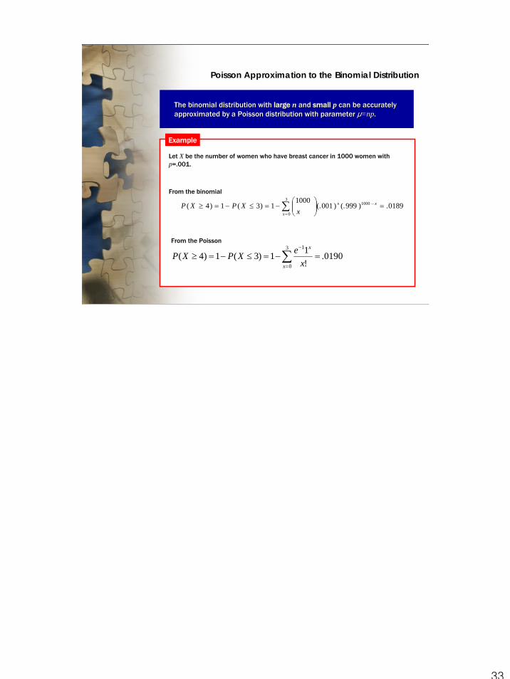
Poisson Approximation to the Binomial Distribution

The binomial distribution with large n and small p can be accurately approximated by a Poisson distribution with parameter μ=np.The binomial distribution with large n and small p can be accurately approximated by a Poisson distribution with parameter μ=np.

Example

Let X be the number of women who have breast cancer in 1000 women with p=.001.

From the binomial

0189.)999(.)001(.1000

1)3(1)4( 10003

0

=⎟⎟⎠

⎞⎜⎜⎝

⎛−=≤−=≥ −

=∑ xx

x xXPXP

From the Poisson

0190.!11)3(1)4(

3

0

1

=−=≤−=≥ ∑=

−

x

x

xeXPXP