DISCRETE DIGITAL FILTER DESIGN FOR MICROELECTROMECHANICAL

SYSTEMS (MEMS) ACCELEROMETERS AND GYROSCOPES

by

Madison E. Martin

A Thesis Submitted to the Faculty of

The Wilkes Honors College

in Partial Fulfillment of the Requirements for the Degree of

Bachelor of Arts in Liberal Arts and Sciences

with a double Concentration in Physics and Mathematics

Wilkes Honors College of

Florida Atlantic University

Jupiter, Florida

May 2010

DISCRETE DIGITAL FILTER DESIGN FOR MICROELECTROMECHANICAL

SYSTEMS (MEMS) ACCELEROMETERS AND GYROSCOPES

by

Madison E. Martin

This thesis was prepared under the direction of the candidate’s thesis advisors, Dr.Marc Hill and Dr. Terje Hoim, and has been approved by the members of her super-visory committee. It was submitted to the faculty of The Honors College and wasaccepted in partial fulfillment of the requirements for the degree of Bachelor of Artsin Liberal Arts and Sciences.

SUPERVISORY COMMITTEE:

Dr. Marc Hill

Dr. Terje Hoim

Dr. Ryan Karr

Dean, Wilkes Honors College

Date

ii

Acknowledgements

I would like to thank Dr. Hill for inspiring this thesis. He has guided me through

all the tribulations associated with completing this study. Most importantly, he was

always willing to tackle my incessant questions as I tried to grasp the concepts in-

volved. Without his guidance I would have been completely lost. I greatly appreciate

all his support throughout this process and through my last three years here. I would

also like to thank Dr. Hoim for her constant reviewing and useful feedback. Her input

has vastly improved my writing skills. Also, I want to thank her for always being an

understanding voice of reason during the most difficult parts of my time here. I would

like to thank both Dr. Hill and Dr. Hoim for shaping my time at Florida Atlantic

University’s Honors College into the most rewarding academic endeavour of my life

thus far.

iii

Abstract

Author: Madison Martin

Title: Discrete Digital Filter Design for Microelectromechanical

Systems (MEMS) Accelerometers and Gyroscopes

Institution: Harriet L. Wilkes Honors College, Florida Atlantic University

Thesis Advisors: Dr. Marc Hill, Dr. Terje Hoim

Concentrations: Physics, Mathematics

Year: 2010

Microelectromechanical systems (MEMS) accelerometers and gyroscopes are small

scale sensors that measure changes in linear acceleration and rotational velocity, re-

spectively. They are fabricated using electronic circuit techniques such as etching

and deposition. MEMS motion sensors can be used in an Inertial Measurement Unit

(IMU) that can be integrated with the Global Positioning System (GPS) to make

a navigation system that is more accurate than each system alone. However, since

MEMS-based IMUs are inherently noisy, we must overcome inaccuracies caused by

the integration of random noise to find position. Accuracy can be increased by ap-

plying digital filters to the data before integration. Comparing the success of finite

impulse response (FIR) filters and infinite impulse response (IIR) filters, we found

that even though our highest order FIR filter yielded the most accurate position,

it was limited by an offset bias in the accelerometer signal and a time delay in the

determined position.

iv

Contents

1 Introduction 1

2 Background 4

2.1 Motion Sensors . . . . . . . . . . . . . . . . . . . . . . . . . . . . . . 4

2.1.1 Accelerometers . . . . . . . . . . . . . . . . . . . . . . . . . . 4

2.1.2 Gyroscopes . . . . . . . . . . . . . . . . . . . . . . . . . . . . 7

2.2 Microelectromechanical Systems . . . . . . . . . . . . . . . . . . . . . 9

2.2.1 MEMS Motion Sensors . . . . . . . . . . . . . . . . . . . . . . 10

2.2.2 Microelectromechanical Systems Fabrication . . . . . . . . . . 13

2.2.3 Microelectromechanical Systems Design . . . . . . . . . . . . . 15

2.3 Discrete Signal Processing . . . . . . . . . . . . . . . . . . . . . . . . 21

2.3.1 Fourier Transforms . . . . . . . . . . . . . . . . . . . . . . . . 21

2.3.2 Discrete Digital Filters . . . . . . . . . . . . . . . . . . . . . . 23

2.4 Numerical Integration . . . . . . . . . . . . . . . . . . . . . . . . . . 27

2.4.1 Riemann Sum . . . . . . . . . . . . . . . . . . . . . . . . . . . 28

2.4.2 Trapezoid Rule . . . . . . . . . . . . . . . . . . . . . . . . . . 30

3 Experiment 32

3.1 Methods . . . . . . . . . . . . . . . . . . . . . . . . . . . . . . . . . . 32

3.1.1 Data Collection . . . . . . . . . . . . . . . . . . . . . . . . . . 32

3.1.2 Data Processing . . . . . . . . . . . . . . . . . . . . . . . . . . 34

3.2 Results . . . . . . . . . . . . . . . . . . . . . . . . . . . . . . . . . . . 37

v

3.2.1 Path 1 . . . . . . . . . . . . . . . . . . . . . . . . . . . . . . . 39

3.2.2 Path 2 . . . . . . . . . . . . . . . . . . . . . . . . . . . . . . . 41

3.3 Discussion . . . . . . . . . . . . . . . . . . . . . . . . . . . . . . . . . 48

3.4 Conclusion . . . . . . . . . . . . . . . . . . . . . . . . . . . . . . . . . 52

Bibliography 57

vi

List of Figures

2.1 Diagram of an accelerometer [6] . . . . . . . . . . . . . . . . . . . . . 5

2.2 Gyroscope [8] . . . . . . . . . . . . . . . . . . . . . . . . . . . . . . . 7

2.3 Diagram of a MEMS gyroscope [6] . . . . . . . . . . . . . . . . . . . 12

2.4 Right sum approach to the Riemann Sum [16] . . . . . . . . . . . . . 29

2.5 Trapezoid Rule [16] . . . . . . . . . . . . . . . . . . . . . . . . . . . . 31

3.1 Cart Setup . . . . . . . . . . . . . . . . . . . . . . . . . . . . . . . . . 33

3.2 Accelerometer Setup . . . . . . . . . . . . . . . . . . . . . . . . . . . 34

3.3 Path 1, from the HC to the HA (created in Google Earth) . . . . . . 38

3.4 Path 2, in the Resident Student parking lot (created in Google Earth) 39

3.5 Velocity determined by Riemann Sum . . . . . . . . . . . . . . . . . . 40

3.6 Position determined by Riemann Sum . . . . . . . . . . . . . . . . . . 41

3.7 Frequency spectrum of the accelerometer’s data while sitting still . . 42

3.8 Frequency spectrum of the data for Path 2 Run 3 . . . . . . . . . . . 43

3.9 Riemann Sum vs. Trapezoid Rule for the raw data . . . . . . . . . . 44

3.10 Riemann Sum vs. Trapezoid Rule for the Chebyshev, of order N = 6,

filtered data . . . . . . . . . . . . . . . . . . . . . . . . . . . . . . . . 45

3.11 Path 2 Run 3 velocity . . . . . . . . . . . . . . . . . . . . . . . . . . 46

3.12 Path 2 Run 3 position using the Riemann Sum . . . . . . . . . . . . . 47

3.13 Path 2 Run 3 acceleration . . . . . . . . . . . . . . . . . . . . . . . . 48

3.14 Path 2 Run 3 frequency . . . . . . . . . . . . . . . . . . . . . . . . . 49

3.15 Path 2 Run 3 velocity for Chebyshev of order 10 filtered acceleration 51

vii

Chapter 1

Introduction

Inertial Navigation Systems (INS) are devices that track real-time motion of what-

ever body they are mounted to. An INS has two main components: an Inertial

Measurement Unit (IMU) and an update system. The IMU measures the real-time

acceleration of the body while the update system changes the position, velocity, and

orientation of the body in reference to the frame in which the body is moving [1].

Since the cost of manufacturing Microelectromechanical Systems (MEMS) is steadily

decreasing, an effort to incorporate MEMS motion sensors in to Inertial Navigation

Systems has arisen. An integrated INS consisting of MEMS-based IMU and a GPS

receiver has the potential to yield very accurate real-time measurements of a body’s

motion. This is because such a MEMS-based IMU is immune to GPS signal jam-

ming or signal loss, while a GPS receiver updates its information more often than

alternative update systems [2]. Such systems are useful for commercial and military

applications. GPS navigation systems are used for driving, running, hiking, and boat-

ing. In fact, many new cars today are equipped with GPS navigation systems. The

military uses highly accurate navigation systems for weapons and air-borne platforms

such as long-range missiles, guided munition, tactical missiles, jets, helicopters, and

unmanned flight vehicles [3]. A MEMS-based INS integrated with GPS may be able

to provide the high accuracy needed for such applications.

Even though MEMS-based INS/GPS are immune to GPS signal loss or jamming,

MEMS inertial sensors are subject to errors associated with both the sensors them-

1

selves and the integration process used to determine position based off of the acceler-

ation data [2]. To improve the accuracy of the integrated result, the raw acceleration

data can be filtered prior to being integrated. The Kalman filter, which works by

predicting a value and performing a weighted average of the predicted and measured

values, is commonly used in MEMS-based INS/GPS [2, 3]. Although it is commonly

used, the Kalman filter has some issues: it requires accurate stochastic modeling and

a priori information of the system [2]. Since stochastic models are models that have

many possible outcomes for a single set of initial conditions, they are difficult to work

with. This requires the outcome of the Kalman filter to be known before, or a pri-

ori, the filter is applied. Finding a priori information is very difficult because it is

practically impossible to accurately know something that has not occurred.

Noureldin et al. dealt with the issues associated with the Kalman filter by us-

ing wavelet decomposition to improve the signal-noise-ratio and compared a Gauss-

Markov (GM) stochastic model (most common) to an auto-regressive (AR) stochastic

model. They found that the AR stochastic model improved the accuracy by 20 percent

when compared to the GM stochastic model. Chen et al. addressed the degradation

of the Kalman filter, due to unknown output commands, by introducing a robust es-

timator that uses fuzzy modeling and filter techniques [4]. Baselga et al. proposed a

data filtering technique that included applying a moving average filter, then applying

a Butterworth filter, then applying a discrete Fourier transform, and lastly applying

a Coiflet 5 wavelet to the MEMS-based IMU data before integrating the IMU with

the GPS update system [5].

In this thesis we will investigate the effect of filtering raw data on the accuracy

of integrated position. We will collect data from a MEMS motion sensor as it is

moved along a known path. The voltage readings will be converted into acceleration

and then filtered. Since it is difficult to find a priori information, we have decided

2

to investigate alternative filtering techniques for MEMS inertial sensors. Instead of

applying the commonly used Kalman filter, we have chose to look at two simpler

types of filter techniques: finite impulse response (FIR) filters and infinite impulse

response (IIR) filters. An FIR can be thought as a non-recursive moving average

than is performed over the signal. An IIR is a recursive filter where each input of

the filtered signal relates to inputs of the non-filtered signal and to other inputs of

the filter signal. The filtered accelerations will be integrated to predict the position

of the device. The integrated position will be compared to the known position, so

that we can determine the accuracy of the filter applied to the device’s data. Our

approach is a more vigorous investigation into the effects of FIR filters and IIR filters

on raw acceleration data. Our results will allow insight into how well FIR and IIR

filtering techniques will work for MEMS motion sensors. Using that insight into how

well FIR and IIR filters work, new filtering techniques could be developed that have

less issues than the Kalman filter, but still have the same level or even a higher level

of accuracy.

The rest of this thesis provides not only background information about MEMS,

motions sensors, and filters, but also provides a more indepth explanation of the ex-

perimental methods, results, discussion and conclusions. We begin with a description

of motion sensors, specifically accelerometers and gyroscopes, on a macro-level. Then

we introduce MEMS by comparing MEMS motions sensors and macro-level motion

sensors. We continue the discussion of MEMS by examining their fabrication meth-

ods, their design process, and their failure analysis. Then, we explain discrete digital

filters and their relation to MEMS motion sensors’ applications. This leads us into the

motivation and specifics of our investigation including methods, results, discussion,

and conclusions.

3

Chapter 2

Background

2.1 Motion Sensors

Inertial sensors are used for a variety of different applications including airbag

control systems, vehicle dynamics, and navigation systems. Inertial sensors convert

physical occurrences into an electrical signal. Such physical occurrences include linear

and rotational motion. Accelerometers are linear inertial sensors and gyroscopes

are rotational inertial sensors. Both devices transfer displacement into an electrical

output.

2.1.1 Accelerometers

Although there are a variety of different accelerometers adapted for applications,

the general design concept is the same. An accelerometer is to converts linear motion

into a readable electrical signal. An accelerometer has four basic components: the

seismic mass, the elastic spring, the dashpot, and the transduction method.

4

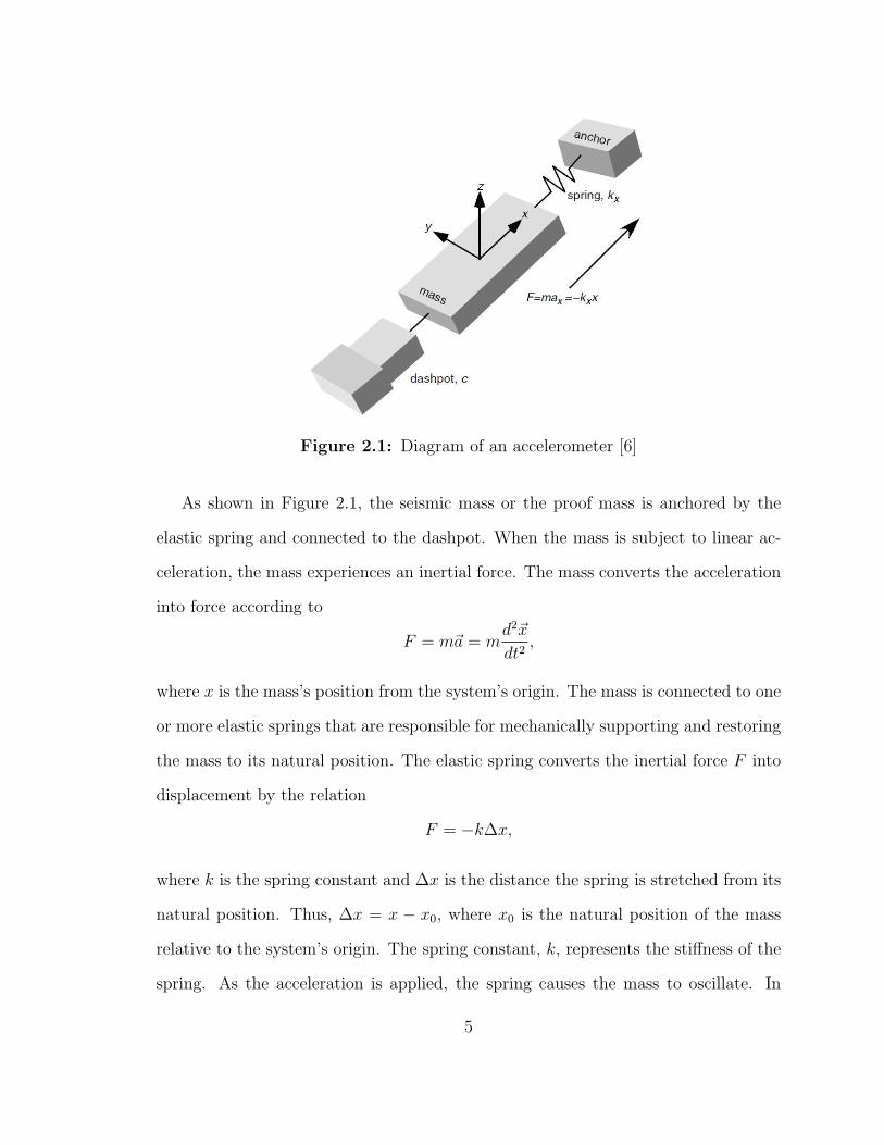
Figure 2.1: Diagram of an accelerometer [6]

As shown in Figure 2.1, the seismic mass or the proof mass is anchored by the

elastic spring and connected to the dashpot. When the mass is subject to linear ac-

celeration, the mass experiences an inertial force. The mass converts the acceleration

into force according to

F = m~a = md2~x

dt2,

where x is the mass’s position from the system’s origin. The mass is connected to one

or more elastic springs that are responsible for mechanically supporting and restoring

the mass to its natural position. The elastic spring converts the inertial force F into

displacement by the relation

F = −k∆x,

where k is the spring constant and ∆x is the distance the spring is stretched from its

natural position. Thus, ∆x = x − x0, where x0 is the natural position of the mass

relative to the system’s origin. The spring constant, k, represents the stiffness of the

spring. As the acceleration is applied, the spring causes the mass to oscillate. In

5

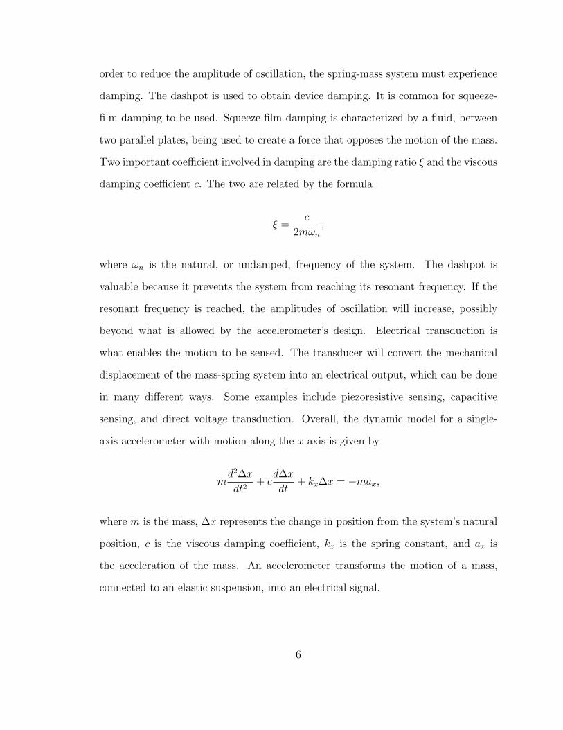
order to reduce the amplitude of oscillation, the spring-mass system must experience

damping. The dashpot is used to obtain device damping. It is common for squeeze-

film damping to be used. Squeeze-film damping is characterized by a fluid, between

two parallel plates, being used to create a force that opposes the motion of the mass.

Two important coefficient involved in damping are the damping ratio ξ and the viscous

damping coefficient c. The two are related by the formula

ξ =c

2mωn,

where ωn is the natural, or undamped, frequency of the system. The dashpot is

valuable because it prevents the system from reaching its resonant frequency. If the

resonant frequency is reached, the amplitudes of oscillation will increase, possibly

beyond what is allowed by the accelerometer’s design. Electrical transduction is

what enables the motion to be sensed. The transducer will convert the mechanical

displacement of the mass-spring system into an electrical output, which can be done

in many different ways. Some examples include piezoresistive sensing, capacitive

sensing, and direct voltage transduction. Overall, the dynamic model for a single-

axis accelerometer with motion along the x-axis is given by

md2∆x

dt2+ c

d∆x

dt+ kx∆x = −max,

where m is the mass, ∆x represents the change in position from the system’s natural

position, c is the viscous damping coefficient, kx is the spring constant, and ax is

the acceleration of the mass. An accelerometer transforms the motion of a mass,

connected to an elastic suspension, into an electrical signal.

6

2.1.2 Gyroscopes

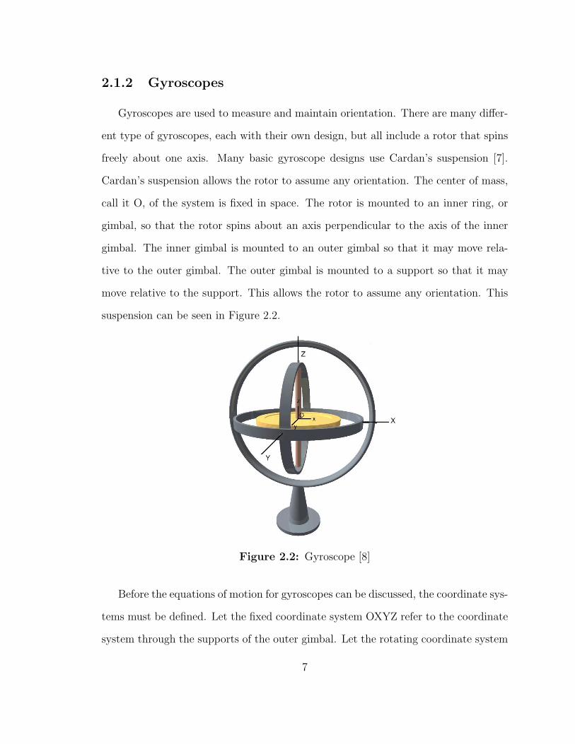
Gyroscopes are used to measure and maintain orientation. There are many differ-

ent type of gyroscopes, each with their own design, but all include a rotor that spins

freely about one axis. Many basic gyroscope designs use Cardan’s suspension [7].

Cardan’s suspension allows the rotor to assume any orientation. The center of mass,

call it O, of the system is fixed in space. The rotor is mounted to an inner ring, or

gimbal, so that the rotor spins about an axis perpendicular to the axis of the inner

gimbal. The inner gimbal is mounted to an outer gimbal so that it may move rela-

tive to the outer gimbal. The outer gimbal is mounted to a support so that it may

move relative to the support. This allows the rotor to assume any orientation. This

suspension can be seen in Figure 2.2.

Figure 2.2: Gyroscope [8]

Before the equations of motion for gyroscopes can be discussed, the coordinate sys-

tems must be defined. Let the fixed coordinate system OXYZ refer to the coordinate

system through the supports of the outer gimbal. Let the rotating coordinate system

7

Oxyz refer to the coordinate system through the inner gimbal. The position of the

rotor is defined by three angles called the Eulerian Angles. The angle of procession,

φ, is the angle the rotor is rotated about the Z-axis. The angle of nutation, θ, is the

angle the rotor is rotated about the Y-axis. The angle of spin, ψ, is the angle the rotor

is rotated about the z-axis. Thus, φ, θ, and ψ are the rates of procession, nutation,

and spin, respectively. Procession occurs if the gyroscope is supported loosely at a

point and the gyroscope rotates slowly about the supporting point like a spinning top

as it slows down, but before it falls over. Nutation is the slight irregular motion in

rotation about the Y-axis. The rates of procession, nutation, and spin relate to each

other when describing the motion of the rotor.

Now, the characteristic equations of the rotor’s motion can be outlined. The

angular velocity with respect to OXYZ is calculated by using

~ω = −φ sin θ~i+ θ~j + (ψ + φ cos θ)~k,

where θ angle of nutation, φ is the rate of procession, θ is the rate of nutation, and ψ

is the rate of spin. The angular velocity of the rotating coordinate system is given by

~Ω = −φ sin θ~i+ θ~j + φ cos θ~k,

where θ, φ, θ, ψ are the same as above. The angular momentum about the center of

mass O is given by

~H0 = −I ′φ sin θ~i+ I ′θ~j + I(ψ + φ cos θ)~k,

where I is the moment of inertia of rotor about the Z-axis and I ′ is the moment of

inertia of the rotor about the transverse axis through O, which is either the X-axis

8

or the Y-axis. The moment about O is defined by

∑~M0 = (~H0)Oxyz + ~Ω× ~H0,

where (~H0)Oxyz is the rate of change of the angular momentum about O with respect

to Oxyz, ~Ω is the angular velocity of the rotating coordinate system, and ~H0 is the

angular momentum about O. These equations define the motion of the rotor of a

gyroscope.

2.2 Microelectromechanical Systems

Inertial sensors can be used for a variety of different applications. Accelerometers

are used in vehicles, machines, electric devices, and structures subject to dynamic

loads. Gyroscopes are commonly used in navigation systems, autopilot applications,

and compasses. Some modern uses for inertial sensors require the sensors to be on

the micro-scale, or below the limits of human perceptions. These uses may require

Microelectromechanical Systems (MEMS) accelerometers and gyroscopes. MEMS are

more than just miniature systems that are on scales below the limits of human per-

ception. “MEMS is simultaneously a toolbox, a physical product, and a methodology,

all in one” [9]. MEMS includes the methodology, process and tools used to design

and create miniature systems. MEMS are also the miniature systems created. At

this point MEMS can be confused with micromachined systems, which is defined as

the design, tools, and fabrication methods to create structures on the microscale [9].

It is true that micromaching is used to make components of MEMS, but not the

entire systems. MEMS requires not only micromachining technologies, but also the

use of common fabrication processes used for electronics. Such technologies include

9

different forms of etching, deposition, and lithography. MEMS also refer to integrated

systems made up of individual Microelectromechanical devices. These larger systems

integrate smaller functions together so that the system is capable of more functions

than the individual devices alone [9]. MEMS not only refers to the device created

by micromaching and electronics technologies, but also refers to the design, creation,

and tools used to create such devices.

2.2.1 MEMS Motion Sensors

MEMS Accelerometers

The design of a MEMS accelerometer is similar to the design of a macro-scale

accelerometer. The design includes the same basic components: the seismic mass,

the suspension element (the elastic spring), the damping function, and the sensing

element [10]. The components in the MEMS accelerometer have the same function

as in the macro-scale accelerometer. There are several important considerations for a

MEMS accelerometer that are not as vital in a macro-scale accelerometer. In order to

avoid amplitude distortion, the accelerometer must amplify all the signals of different

frequencies equally [10]. In order to avoid phase distortion, the harmonic components

of the signal must shift equally with time. Usually, phase distortion is eliminated

with a damping ratio ξ ∼= 0.7 [10]. It is also important that the accelerometer

never reach resonant frequency, which would result in increased amplitude beyond

the constraints of the device. In order to ensure that the accelerometer does not

reach resonant frequency, the accelerometer’s natural frequency must be at least an

order of magnitude higher than the largest frequency the device can sense. Overall,

the basic schematic of a MEMS accelerometer is similar to that of a macro-scale

accelerometer, but there are different issues to consider in the design process.

10

MEMS Gyroscopes

The design of a MEMS gyroscope differs from the design of a macro-scale gyro-

scope, but is somewhat similar to an accelerometer’s design. MEMS gyroscopes in-

clude a mass attached to a suspension element that anchors the mass to the substrate.

The gyroscope also includes a sensing method. In order for a measurable signal to be

generated, MEMS gyroscopes must include the oscillation of the mass [6]. Thus, most

MEMS gyroscopes are vibrating mass gyroscopes. In a vibrating mass gyroscope, the

mass oscillates about one axis while rotating about the central axis [10]. Due to

this vibratory motion occurring while in rotation, the mass is subject to the Coriolis

effect. This means that there is an additional component of acceleration, known as

the Coriolis acceleration, defined by

ac = 2~Ω× ~v,

where ~Ω is the angular velocity of the mass, and ~v is the velocity relative to the

rotating frame of reference [7]. The Coriolis acceleration causes the mass to deflect

in the axis perpendicular to the axis of oscillation, but still within the plane on

oscillation. The sensing method detects the deflection of the mass due to the Coriolis

acceleration [10]. A diagram of a MEMS gyroscope can be found in Figure 2.3.

11

Figure 2.3: Diagram of a MEMS gyroscope [6]

When designing a vibratory MEMS gyroscope, it is important to consider the

quadrature error. Quadrature error refers to the deflection in the axis perpendicular

to the plane in which the mass oscillates, caused by imbalances in the vibration of the

mass [10]. In order to compensate for quadrature error, changes in the Coriolis effect

must cancel out the imbalance in the vibration of the mass. Consider a vibrating

gyroscope whose mass rotates about the z-axis and oscillates about the y-axis. The

equation for such a gyroscope is

d2x

dt2+ 2ξxωnx

dx

dt+ ω2

nxx = 2Ωzdy

dt,

where x is the position of the mass along the x-axis, ξx is the damping ratio in the

x-axis, ωnx is the natural frequency of the device in the x-axis, Ωz is the rate of

rotation about the z-axis, and dydt

is the velocity in the y-axis [6]. In order for a

MEMS gyroscope to have a measurable signal, it is necessary for the mass to oscillate

about one axis and rotate about a different axis.

12

2.2.2 Microelectromechanical Systems Fabrication

Applications

As previously stated, the term MEMS incorporates not only the micro-machined

device that is created using electrical fabrications methods, but also refers to the

design, creation, and tools implemented in the making of the device. MEMS are also

integrated with other devices to increase their usefulness. They are used in many

different applications, but among the most common and well known are automotive

uses and ink-jet printer uses. MEMS accelerometers are used for sensing the necessity

of automotive air-bag deployment [9]. Other MEMS sensors are used to sensor tire

pressure [9]. One of the most frequent applications of MEMS is their use in ink-jet

printer heads [11]. The future market of MEMS applications will continue to grow

as fabrication processes increase in sophistication. This will cause a reduction in cost

of MEMS, making them more economical to produce on a large scale. For example,

the use of batch fabrication, the manufacturing of many identical parts, will become

more effective for MEMS applications [9]. In addition to improving the economical

success of MEMS, more applications are being developed such as bioMEMS, rfMEMS,

and opticals MEMS [11]. BioMEMS is an application of MEMS to biological studies.

RfMEMS includes wireless devices that use MEMS. A micromirror is an example of an

optical MEMS. The market of MEMS will continue to grow through the development

of more cost effective methods of production and finding more applications.

Materials

Part of what makes MEMS devices different from other mirco-machined devices

is the types of materials used to create them. Three electrical properties are im-

13

portant for the fabrication of MEMS devices: piezoresistivity, piezoelectricity, and

thermoelectricity. Piezoresistivity is the change in electrical resistance in response

to mechanical stress [9]. Piezoelectricity refers to the production of an electric field

in response to an external force [9]. Thermoelectricity refers to relationship between

temperature changes and electrical potential [9]. It can refer to either a temperature

difference creating an electrical potential or an electrical potential creating a tem-

perature difference. Many of the materials used in MEMS have one or more of the

preceding electrical properties. Some of the more commonly used materials include

silicon-compatible materials such as silicon, silicon oxide, and nitride [9]. These ma-

terials have good electrical and thermal conductivity. MEMS also use glass, fused

quartz, and diamond. Quartz is piezoelectric and electrically insulating [9]. Poly-

mers are used in MEMS for their versatility. For example, thermoplastics are used

for their ability to re-harden upon cooling [9]. These materials, and others, are used

to produce thin metal films that are used in MEMS. Piezoelectric films are mostly

used in electromechanical transducers like those in MEMS accelerometers [12]. The

materials used in MEMS are commonly materials that possess valuable thermal and

electrical properties.

Process

The thin metal films used in MEMS are fabricated using deposition, etching, and

lithography. Deposition methods deposit uniform layers of the desired materials to

create the thin films. Sputter deposition works by bombarding a target, made of the

desired material with a wafer on it, with a flux of inert gas [9]. Chemical vapor de-

position involves the use of a chemical reaction to deposit the layers of material [10].

Etching is commonly used in microelectronics “to depress a design pattern into ma-

terial” [10]. The etching can be done with chemicals, as in wet chemical etching,

14

or physically, as in ion milling etching. Ion milling etching uses noble gases with

significant mass to etch the design [10]. Plasma etching is used often in MEMS. The

plasma provides a flux of radicals, neutral particles, electrons and ions on the surface

to be etched, which allows for a combination of chemical and physical etching pro-

cess [10]. Lithography involves illuminating a shutter above a mask that resides over

a photosensitive wafer. This transfers the image from the mask to the wafer [10]. De-

position, etching, and lithography are used in integrated processes, such as sacrificial

surface micromachining and bulk micromachining, to create larger MEMS structures.

Sacrificial surface micromachining produces structures by deposition and etching of

structural and sacrificial thin films [10]. Bulk micromachining creates structures by

using chemical and physical deposition of a silicon substrate [10]. It is the deposi-

tion, etching, and lithography processes that create the thin films for MEMS that

distinguish MEMS from micro-machined devices, which do not use such methods.

2.2.3 Microelectromechanical Systems Design

When it comes to creating a MEMS device, engineers follow a general method-

ology. First, they analyze the general principles of use. Then they run computer

simulations of the device. Once completed, the device is then fabricated. To ensure

the device is successful, they repeat the steps until the device is well designed and

can be fabricated on a large scale [9]. There are components that are frequently used

in MEMS device design such as actuators, optical elements, mechanical coupling el-

ements, and electrical elements [10]. These are referred to as standard components

and they have already been designed, fabricated, and tested [10]. It is common for

such components to be used in further MEMS design.

15

Design Rules

When engineers draft a design for a MEMS device, they must consider design

rules “that enable communication between the fabrication engineer and the design

engineer” [10]. These rules have to do with possible manufacturing issues that could

occur during the previously mentioned fabrication methods. According to Allen,

the designer must consider patterning limits and material stability for all fabrication

methods [10]. Patterning limits, or critical dimensions, refer to the smallest feature

that can be realized by the device. The stability of the material must meet specific

requirements before the device can be fabricated. Allen asserts that when fabricating

thin films using forms of etching, the engineer must take into consideration etch

pattern uniformity, etch compatibility, etch precision, layer anchoring, and created

debris [10]. It is important to attempt to achieve etch pattern uniformity and to

align the masks relative to one another for finite precision. The etch pattern that is

to be done must be compatible with the material to be used. When etching layers

of materials, it is vital that the layers are properly anchored to each other. During

etching there could be debris produced, which is referred to as stringers. Another

type of debris, called floaters, include debris that is not attached to the material and

usually is contained with another structure. Chemical etching methods must include

etch release holes that allow the etchant to reach the material [10]. When fabricating

thin films using lithography, the design engineer must consider the depth of focus.

The fabrication needs to be done within that depth, otherwise it is likely that the

lithography will fail [10]. When using Sacrificial surface micromachining to produce

structures, it is common for dimples, small bumps on the underside of the layers of

material, to prevent large area surface contact [10].

When the design rules are checked, there are two classifications of violations:

16

design rule advisory and design rule error. Design rule advisory refers to a violation

that the design engineer needs to evaluate and address [10]. Design rule error refers to

violations that need mandatory and immediate evaluation [10]. An engineer creating

a new MEMS device will likely use standard components in his design as well as

consider design rules.

Design Analysis and Modeling

After drafting a design for a MEMS device, the design engineers will analyze

the device. They will model the device at three different stages: a design synthesis

model, a detailed design model, and a macromodel. The design synthesis model is a

simple model of low order and low degrees of freedom. The design synthesis model

includes important parameters and their interaction, as well as the device’s sensitivity

to variables [10]. Fundamental physical principles are applied to the design synthesis

model. The detailed design model is of higher order and has a large number of de-

grees of freedom. This includes numerical modeling, where differential equations of

the model are replaced with approximate algebraic equations [10]. There are three

different types of numerical modeling: finite difference modeling, finite element mod-

eling, and boundary element modeling. In finite difference modeling, the domain is

approximated using finite difference approximation at each node [10]. Finite element

modeling includes replacing the differential equations with integral equations using

the subdomain [10]. Boundary element modeling replaces the differential equations

with integral equations. Macromodels are models that are the best representations

of the device in real world use. The process of modeling allows the engineer to test

the device in computer simulations before the device is actually produced.

As with any type of design, there are always design uncertainties that can not be

avoided. Even though devices may be properly designed and analyzed, once produced,

17

the device may not perform as intended. This could be due to number of reasons.

Firstly, it is easier to create a relative design metric rather than an absolute design

metric [10]. This could result in a device that does not work properly in every possible

situation. Also, there is the idea of relative tolerance which refers to the feature size

of the device divided by the part size of the device [10]. The tolerances of fabrication

methods and the ability of the device to meet the design metrics are related to the

relative tolerance of the device [10]. Every MEMS device has a certain element of

design uncertainty.

Failure Analysis

An important feature of MEMS design and analysis that has not yet been men-

tioned is MEMS reliability. The reliability of a MEMS device refers to the “ability of

a device to perform a required function for a specified amount of time” [10]. Reliabil-

ity depends on power supply, packaging of the device, any subsystems in the device,

and any software or coding required for the device to run [10]. Some commonly used

terms in reliability analysis include method of operation, failure, and some statistics

terms such as sample size and plots. The method of operation of a device, refers to

the detailed definition of the devices operation [10]. The general definition of failure

is “a change in the performance of a component or system resulting in the inabil-

ity to use the component or system as designed or intended” [12]. The specifics of

what counts as failure depends on the device [10]. Statistics are commonly used to

analyze failure and reliability. It is important for the sample size to be large enough

for the reliability test to be statistically significant. Usually, probability is used, so

cumulative probability distribution plots are important. It is common for the total

number of failures to be plotted against the operation time in the cumulative failure

distribution plot [10]. Another common plot is the failure frequency distribution plot,

18

which graphs the failure rate versus time [10]. Reliability considerations and analyses

are important for MEMS design.

In order for failure analysis to yield minimal issues, engineers consider reliability

in their design of MEMS devices. Firstly, a MEMS device is placed into one of four

classes of the MEMS Device Taxonomy [10]. Class 1 includes devices that have no

moving parts. Class 2 includes devices that have moving parts with no impacting

or rubbing surfaces. Class 3 includes devices that have moving parts and impacting

surfaces but not rubbing surfaces. Lastly, class 4 includes devices that have moving

parts with impacting and/or rubbing surfaces. There is a Product-Reliability Issue

Matrix that discusses the possible reliability issues of each class of MEMS device.

These issues in addition to packaging and failure prevention are considered in the

design of a MEMS device. Usually, the design of a device can compensate for a

specific part’s failure with the design of other parts [10]. When packaging MEMS in-

ertial sensors, the packaging must provide electrical connections, electrical isolations,

mechanical support, and must isolate stress and dissipate heat through thermal con-

duction [10]. Failure prevention includes considering failure modes and their effects

in critical analysis [10].

Major MEMS failure modes include operational failure mechanisms, environmen-

tal failure mechanisms, and degradation mechanisms. Operational failure mecha-

nisms include wear, fracture, fatigue, charging, creep, and stiction [10]. Wear refers

to removal of material from a surface because of mechanical action. Fracture is the

breaking up of a surface due to environmental force or an interaction. Fatigue refers

to the weakness in a structure because of cyclical actions, like in an oscillatory de-

vice. Charging only occurs in devices that contain dielectric materials, which make

the device susceptible to changes in voltage. Creep refers to plastic strain over time,

the slow movement of atoms under stress, and is important for thin metal layers.

19

Stiction occurs if surfaces come into contact because surface forces become the dom-

inant forces. Environmental failure mechanisms include shock, vibration, thermal

cycling, humidity, radiation, and electrostatics discharge [10]. Shock refers to a single

event, due to environmental forces, that cause an issue with the device’s performance.

Vibration is a continuous force or displacement excitation that occurs because of en-

vironmental forces. Thermal cycling refers to the thermal strain between materials

that have different coefficients of thermal expansion. Humidity can cause conden-

sation which creates capillary forces that can lead to stiction. Radiation can cause

material damage to a MEMS device. If MEMs are not handled correctly, they can

experience an electrostatic discharge. Degradation mechanisms are subtle failures

that occur from operational and environmental mechanisms that, over long periods

of time, alter the device’s performance enough to cause the device to fall out of specifi-

cations [10]. In addition to operational, environmental, and degradation mechanisms,

failure can be caused by weakness in the design of the MEMS device and variations

in the production of the device [9].

The failure analysis of a MEMS device includes testing the devices for possible

failures. The goal is to identify what causes each particular failure. Usually MEMS

device failures are caused by one or more of the previously mentioned failure modes.

Once the cause is identified, the next step is to determine what are the critical features

or parameters of the device, or part of the device, that need to be modified [12]. It

is common for engineers to use a fault tree approach to analyze failures. Usually, a

Failure Modes, Effects, and Critical Analysis (FMECA) worksheet is filled out about

each failure. The FEMCA worksheet includes the mode of operation of the device,

the failure modes, the specific failure mechanism, what caused the failure, the effects

of the failure, and the rating of how critical the failure is [10]. The final step of failure

analysis is to redesign the MEMS device so that the failure will not occur again.

20

2.3 Discrete Signal Processing

Microelectromechanical systems motion sensors output readings that represent

the acceleration experienced by the device over a time period. Therefore, our output

signal is a discrete-time signal that we must process before we can determine velocity

and position from the signal.

In order to analyze the frequency response of the device, we have to take the

discrete time signal and turn it into a signal in the frequency domain. This is ac-

complished by applying a Fourier Transform to our signal. Several different types

of Fourier Transforms that are appropriate for discrete signals are discussed within

the next section. These include the Discrete-Time Fourier Transform (DTFT), the

Discrete-Fourier Transform (DFT), and the Fast Fourier Transform(FFT).

Since the output signal of MEMS motion sensors are subject to noise, we have to

reduce the noise before determining velocity and position from the signal. Discrete

digital filters can be applied to a signal to smooth out the signal, or remove the noise

associated with a signal. A digital filter can be thought of as an averaging operation

that smooths its input signal [13]. We will discuss finite impulse response (FIR) filters

and infinite impulse response (IIR) filters in Section 2.3.2

2.3.1 Fourier Transforms

In the context of discrete signal processing, Fourier Transforms (FT) are opera-

tions that convert a time signal from the time domain into the frequency domain. The

result of a Fourier Transform describes the frequencies included in the original time

signal. The result is always periodic regardless of the original signal being periodic

or not.

21

The Discrete-Time Fourier Transform

The Discrete-Time Fourier Transform (DTFT) requires a discrete input signal,

which makes this FT applicable to the signals outputted by MEMS motion sensors.

The discrete time signal does not have to be periodic for the DTFT to be applied.

The signal could be of infinite length. The DTFT is determined by

X(ejω) =∞∑

n=−∞

x(n)e−jωn,

where x(n) is the original signal and ω = 2πf is the angular frequency [14]. If we have

information about the frequency spectrum of the original signal, we could determine

the original signal by applying the Inverse Discrete-Time Digital Fourier Transform

(IDTFT). The IDTFT is determined by

x(n) =1

2π

∫ π

−πX(ejω)ejωndω,

where X(ejω) is the result of the DTFT and ω = 2πf is the angular frequency [14].

The Discrete Fourier Transform

The Discrete Fourier Transform (DFT) works in very much the same way as the

DTFT. The DFT requires that the input signal be discrete, but in this case the

signal also has to be periodic. It is necessary for the input signal to be of finite

length, so we can represent the original signal as x(n) : n = 0, 1, . . . , N − 1. The

DFT is determined by

X(k) =N−1∑n=0

x(n)e−j(2πN )kn,

22

where x(n) is the original signal of length N and ωk =(

2πNk)

corresponds to the kth

frequency of the signal [14]. The original signal can be determined from the results

of a DFT by applying the Inverse Discrete Fourier Transform (IDFT). The IDFT is

determined by

x(n) =1

N

N−1∑n=0

X(k)ej(2πN )kn,

where X(k) is the result from the DFT [14].

Fast Fourier Transform

The Fast Fourier Transform (FFT) is an slightly altered version of the DFT. The

FFT takes advantage of the symmetric and periodic properties of e−j(2πN )kn [13]. The

FFT is just an algorithm that can be carried out quicker than the DFT. It reduces the

amount of calculations by choosing N such that N = r1r2 . . . rm, where r is an integer

called the radix. One of the more useful choices for N is N = rm. The FFT is quicker

than the DFT, because for a signal of length N , the DFT requires N2 multiplications

while FFT requires N2

log2N multiplications [14]. Even though the FFT is a quicker

algorithm than the DFT, they both yield the same result.

2.3.2 Discrete Digital Filters

Discrete digital filters are algorithms that can be applied to discrete signals and

act as a smoothing operation by removing unwanted frequencies or passing desired

frequencies. Discrete digital filters are advantageous because of their immunity to

noise, high accuracy, and ability to be modified easily [13]. Typical digital filters

function act as low pass filters, high pass filters, band pass filters, and bandstop

filters [14]. Low pass filters allow low frequencies and block high frequencies. High

pass filters allow high frequencies and block low frequencies. Bandstop filters allow

23

specific intermediate frequencies. There are two main types of discrete digital filters:

infinite impulse response (IIR) filters and finite impulse response (FIR) filters.

Infinite Impulse Response Filters

Infinite impulse response filters are recursive filters, where the filter’s impulse

response has the potential to be of infinite duration. An Nth order, or filter length

of N , IIR filter of x(n) is represented as

y(n) +A1y(n− 1) + . . .+ANy(n−N) = B0x(n) +B1x(n− 1) + . . .+BMx(n−M),

where x(n) is the original signal and y(n) is the filtered signal [13]. Even though IIR

filters need signals of smaller length (than FIR filters), they are not always stable.

The type of IIR filter we will be using is the Chebyshev II filter. The Chebyshev

II filter makes use of the Chebyshev polynomials given by

Tn(x) = cos(n cos−1 x),

where Tn(x) is the polynomial fit of degree n. This class of polynomials has an

equiripple property, where Tn(x) oscillates about zero with its maximum and mini-

mum equal to ±1. The goal of Chebyshev filters is to have the response be maximally

flat, which requires the maximum and minimum of the errors to have equal magni-

tude, or be equiripple. The Chehyshev II filter, or the inverse Chebyshev filter, can

be represented as

|H(v)|2 = 1−∣∣∣∣Hc

(1

v

)∣∣∣∣2 ,where Hc

(1v

)is the nth order Chebyshev I filter with the highpass transformation

24

v →(

1v

)[13]. If we let ∣∣∣∣Hc

(1

v

)∣∣∣∣2 =

(1

ε2T 2n

(1v

)) ,we get

|H(v)|2 =ε2T 2

n

(1v

)1 + ε2T 2

n

(1v

) .If we divide both the numerator and the denominator by ε2T 2

n

(1v

), we get

|H(v)|2 =1

1 +

[1

ε2T 2n( 1

v )

] .

If we let L2n(v) = 1

ε2T 2n( 1

v ), we get

|H(v)|2 =1

1 + L2n(v)

,

where L2n(v) is a rational function rather than a polynomial function [13]. The stop-

band edge is νs and the passband edge is νp. For the Chebyshev II filter, the stopband

edge is normalized such that vs = 1 = ωsωs

and vp = ωpωs

, where ωs is the normalized

stopband edge freqency and ωp is the passband edge frequency. The stopband edge

ripple factor is 1ε2

, where the filter gain is maximum at the stopband edge when

|H(1)|2 =1

1 + 1ε2

and the filter gain has a minimum of 0. The Chebyshev II filter is similar to the

Chebyshev I filter because it uses the equiripple nature of the Chebyshev polynomials.

Chebyshev II filter improves the filter delay by using a frequency transform to transfer

the ripple to a frequency outside of the passband [13]. Overall, the Chebyshev II

filter exhibits equiriple behavior in the stopband and has a monotonic response in the

25

passband.

We will be performing a Chebyshev II filter by using the [b, a] = cheby2(n,R,Wst)

command in MATLAB, where n is the filter order, R is the stopband ripple (in dB)

down from the peak passband, and Wst is the normalized stopband edge frequency.

The normalized stopband edge frequency is a number btween 0 and 1, where 1 cor-

responds to half of the sampling frequency. This command works by designing a

lowpass Chebyshev II filter with those parameters. We apply the filter to our signal

by using the y = filter(b, a,X) command that filters the vector X with numerator

coefficient b and denominator coefficient a. MATLAB filters X by using a direct

form II transposed implementation of the standard difference equation. Through the

use of [b, a] = cheby2(n,R,Wst) and y = filter(b, a,X), we are able to design and

implement our own Chebyshev filters.

Finite Impulse Response Filters

Finite impulse response filters are non-recursive filters, where the filter’s impulse

response is of finite duration. The FIR filter can be considered a weighted sum, or

moving average of past and present inputs [13]. An Nth, or filter length of N , order

FIR filter is represented as

y(n) = B0x(n) +B1x(n− 1) + . . .+BMx(n−N),

where Bk are the coefficients, x(n) is the original signal and y(n) is the filtered

signal [13]. Even though FIR filters are always stable, they require a larger filter

length than IIR filters. In general, a FIR filter design consists of a window based

design, where windows are created using the impulse response of ideal filters. Win-

dowing involves the multiplication of the filter’s impulse response by a rectangular

26

window [13]. Generally the window width is equivalent to the filter’s order. The

next step in designing a FIR filter is frequency sampling with an arbitrarily chosen

cut-off frequency [13]. The optimal design of an FIR filter minimizes the maximum

approximation errors while allowing for the smallest filter length.

For our purposes, we applied FIR filters by using the MATLAB command b =

fir1(n,Wn) to get the coefficients of the filter and then using the command y =

filter(b, a,X) to filter the data. The fir1 command works by computing the coefficients

b for a low pass FIR filter of order N and normalized cut-off frequency Wn. The low

pass FIR filter, in this case, is window based filter such that

b(n) = w(n)h(n),

for 1 ≤ n ≤ N , where w(n) is the window and h(n) is the inverse Fourier transform

of the ideal frequency response. The MATLAB command y = filter(b, a,X) works

by filtering the data in vector X with numerator coefficient b and denominator co-

efficient a. The filter that MATLAB applies for this command is a direct form II

transposed implementation of the standard difference equation. Through the use of

b = fir1(n,Wn) and y = filter(b, a,X) in MATLAB, we were able to design our own

FIR filters.

2.4 Numerical Integration

Inertial Navigations Systems track the real time acceleration, velocity, and position

of a moving body. If a MEMS-based IMU is used, the electrical output, once converted

into acceleration, must be integrated to get velocity and position. This is done after

a digital filter is applied to the signal. If we have an acceleration function a(t), a

27

velocity function v(t), and a position p(t), they can be related as follows:

∫a(t) = v(t)

and ∫v(t) = p(t).

Since for a discrete-time signal we do not have a definable function, we need to use

numerical integration methods to estimate the previously mentioned integrals. The

two numerical integration methods we will be discussing are the Riemann Sum (in

Section 2.4.1) and the Trapezoid Rule (in Section 2.4.2).

2.4.1 Riemann Sum

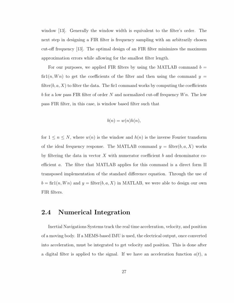
The Riemann Sum definition of a definite integral is

∫ b

a

f(x)dx = lim∆x→0

∑i

f(xi)∆x,

where [a, b] is divided into subdivisions of width ∆x and xi is the ith subdivision of

[a, b] [15]. The definite integral can be approximated by three versions of the Reimann

Sum: the left sum, the right, and the mid-point. For all three methods [a, b] is divided

into n subdivisions of width ∆x. The left sum is defined as

∫ b

a

f(x)dx = f(x0)∆x+ f(x1)∆x+ . . .+ f(xn−1)∆x,

where f is evaluated at the left endpoint of each subdivision. The right sum is defined

as ∫ b

a

f(x)dx = f(x1)∆x+ f(x2)∆x+ . . .+ f(xn)∆x,

28

where f is evaluated at the right endpoint of each subdivision (See Figure 2.4). The

mid-point sum is defined as

∫ b

a

f(x)dx = f

(x0 + x1

2

)∆x+ f

(x0 + x1

2

)∆x+ . . .+ f

(xn−1 + xn

2

)∆x

where f is evaluated at the mid-point of each subdivision.

Figure 2.4: Right sum approach to the Riemann Sum [16]

Consider the equation for the right sum,

∫ b

a

f(x)dx = f(x1)∆x+ f(x2)∆x+ . . .+ f(xn)∆x.

This can be rewritten as

∫ b

a

f(x)dx = ∆x(f(x1) + f(x2) + . . .+ f(xn)).

29

When considering the cumulative right Riemann Sum, the equation becomes

∫ b

a

f(x)dx = ∆x

(f(x1), f(x1) + f(x2), f(x1) + f(x2) + f(x3), . . . ,

n∑n=1

f(xn), . . .

).

This can be done in MATLAB by using the cumsum command as follows

∫ b

a

f(x)dx = ∆xcumsum(f(x)).

The MATLAB command cumsum is just the cumulative sum of the input array,

f(x) in this case. We used the cumsum command twice, as demonstrated below, to

determine velocity and position for the MEMS motion sensors’s acceleration data a(t)

(stored in an array):

v(t) = ∆xcumsum(a(t))

and

p(t) = ∆xcumsum(v(t)).

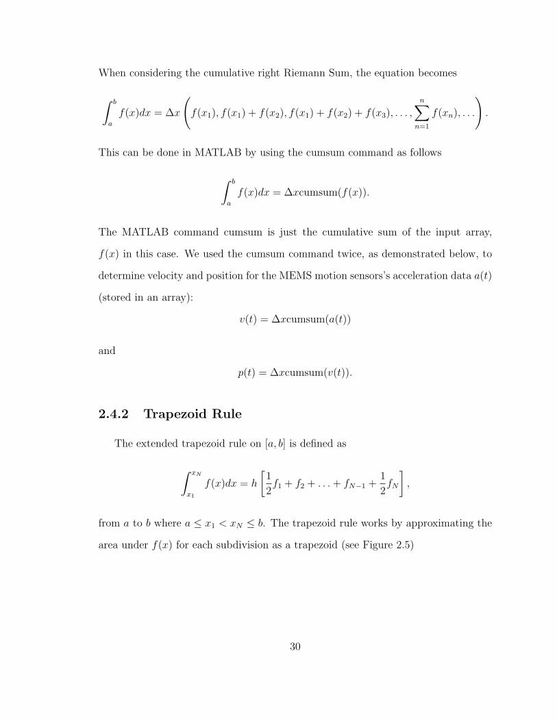
2.4.2 Trapezoid Rule

The extended trapezoid rule on [a, b] is defined as

∫ xN

x1

f(x)dx = h

[1

2f1 + f2 + . . .+ fN−1 +

1

2fN

],

from a to b where a ≤ x1 < xN ≤ b. The trapezoid rule works by approximating the

area under f(x) for each subdivision as a trapezoid (see Figure 2.5)

30

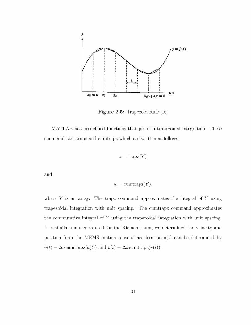
Figure 2.5: Trapezoid Rule [16]

MATLAB has predefined functions that perform trapezoidal integration. These

commands are trapz and cumtrapz which are written as follows:

z = trapz(Y )

and

w = cumtrapz(Y ),

where Y is an array. The trapz command approximates the integral of Y using

trapezoidal integration with unit spacing. The cumtrapz command approximates

the commutative integral of Y using the trapezoidal integration with unit spacing.

In a similar manner as used for the Riemann sum, we determined the velocity and

position from the MEMS motion sensors’ acceleration a(t) can be determined by

v(t) = ∆xcumtrapz(a(t)) and p(t) = ∆xcumtrapz(v(t)).

31

Chapter 3

Experiment

3.1 Methods

In this section, we outline the specifics of our data collection and analyses. First,

we discuss the setup of the experiment and the details of how we collected data.

Then, we discuss how we examined our data. We include the specifics of how we

converted the voltage into acceleration, how we filtered our signal, how we examined

the frequency of our signal, how we integrated our signal, and how we compared our

results.

3.1.1 Data Collection

We connected an Analog Devices iMEMS accelerometer ADXL330 to a National

Instruments DAQpad, so that we could collect data through MATLAB’s Data Acqui-

sition Toolbox. The ADXL330 is a 3-axis sensing MEMS accelerometer that outputs

data in Volts. We set up four channels, one for each axis (x, y, z) and a fourth that

connected only to the DAQpad. The fourth channel allowed us to measure the signal

from just the DAQpad. The DAQpad was connected to a computer that was also

connected to a Garmin handheld GPS receiver. The GPS receiver outputted a string

of simple text that contained time, position, and velocity data. We used the virtual

COM port program Hercules to save the output as a logfile. We mounted this entire

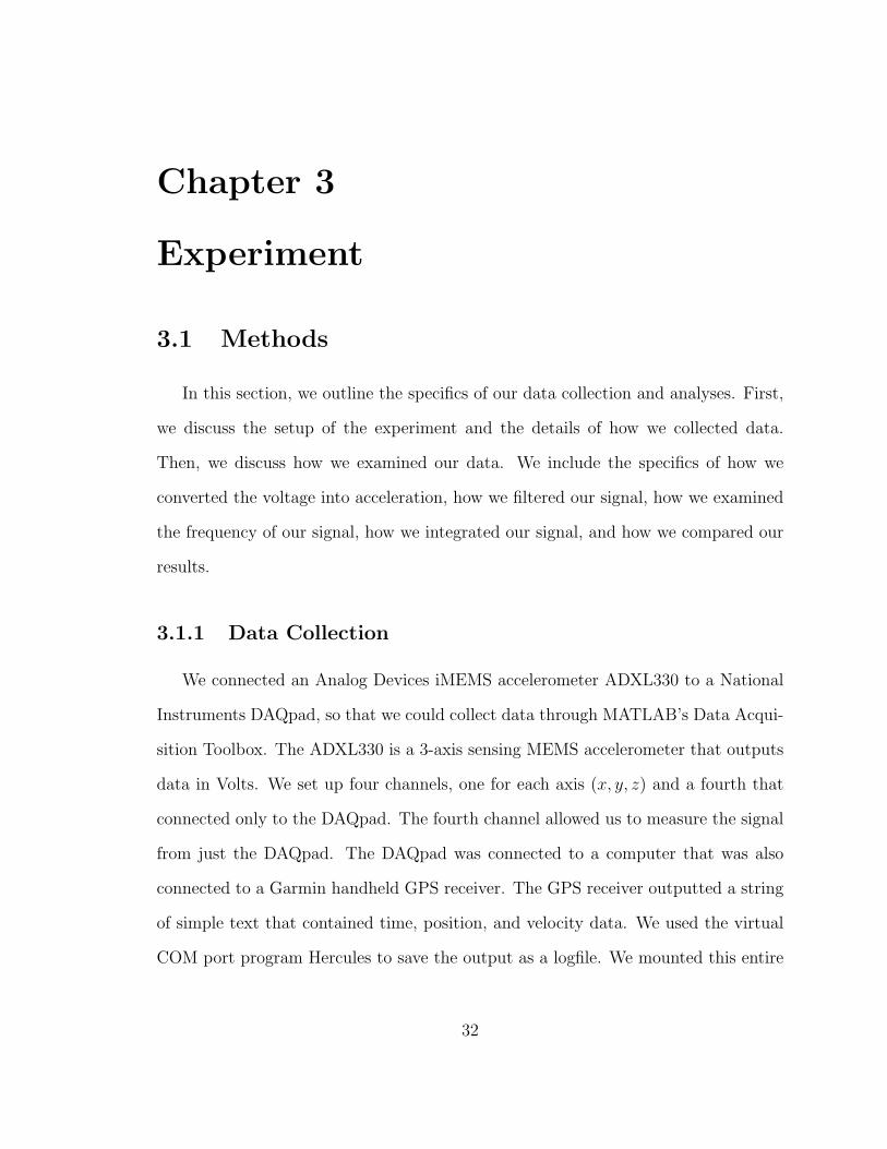
32

setup on a cart as seen in Figure 3.1.

Figure 3.1: Cart Setup

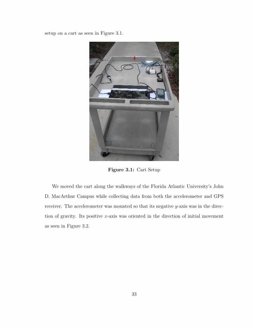
We moved the cart along the walkways of the Florida Atlantic University’s John

D. MacArthur Campus while collecting data from both the accelerometer and GPS

receiver. The accelerometer was mounted so that its negative y-axis was in the direc-

tion of gravity. Its positive x-axis was oriented in the direction of initial movement

as seen in Figure 3.2.

33

Figure 3.2: Accelerometer Setup

Each selected path was repeated five times. We began each run with non-moving

data at the desired origin. Then we moved the cart along the path and ended each

run with non-moving data at the desired end point.

3.1.2 Data Processing

The accelerometer data from the path runs was given in Volts (V) while the

GPS data was given as a string of text. Part of the GPS text was the latitude and

longitude. Assuming the starting point of the path was our origin, we converted the

changes in latitude and longitude into changes in x-position and y-position in meters.

We assumed there was a linear relationship between voltage and acceleration, so that

we could convert the outputted accelerometer voltage to acceleration. Before each

path, we collected non-moving data from the accelerometer with the positive direction

of each axis oriented in the direction of gravity and then with the negative of each

axis oriented in the direction of gravity for a total of six different data matrices.

34

We used this orientation data to determine the slope and offset needed in the linear

equation to convert voltage to acceleration. We did this by assuming the difference

in voltage between the positive and negative orientations of each axis is equivalent to

an acceleration difference of 2g, where g is the acceleration of gravity. The slope of

our linear relationship was determined by

slopex,y,z =2g

〈|V+x,y,z − V−x,y,z|〉,

where V is voltage and 〈〉 represents the average of the quantity inside. This was

done for each axis, so that we had a x-slope, y-slope, and z-slope. The offset of the

linear equation was determined by

offsetx,y,z =

⟨V+x,y,z + V−x,y,z

2

⟩,

where V is voltage and 〈〉 represents the average of the quantity inside. The linear

equation we used to convert the voltage into acceleration (in term of gs) was

ax,y,z = slopex,y,z(data− offsetx,y,z).

Once we converted the data from each path run into acceleration data, we applied

a finite impulse response (FIR) filter to the acceleration data. Using MATLAB, we

created a function that performed a FIR filter of specified order and cutoff frequency

to the inputed data. This function included the MATLAB commands b = fir1(n,Wn)

and y = filter(b, a,X), which we explained earlier. For each path run we applied the

FIR filter with a cutoff frequency Wn = 0.01 (which is equal to 5 Hz) and for four

different orders n (100, 500, 1000, 1500) to the acceleration data. We also applied a

infinite impulse response (IIR) filter to the acceleration data. Using MATLAB, we

35

created a function that performed a Chebyshev filter using the commands [b, a] =

cheby2(n,R,Wst) and y = filter(b, a,X) (explained earlier). For each path run we

applied this function with order n = 6, Wst = 0.01 (5 Hz), and R = 40. We also

examined a Chebyshev filter of order n = 10, Wst = 0.01(5Hz), and R = 40 so that

we could observe the instability of IIR filters. With the four FIR filters and the IIR

filter were able to discuss the differences in performance of the two types of filters.

Before we can integrate the acceleration data to get velocity and position, we had

to offset the data to account for any shifts in the gravity vector of the system. We

determined the offset for each subdivision of motion by averaging all of the accel-

eration data for the initial non-moving section, the moving middle section, and the

final non-moving section. We subtracted those averages from each data point in the

corresponding motion section. We repeated this process for the raw data and each

matrix of filtered data. We then used these adjusted acceleration matrices for our

analysis.

In order to determine position from the acceleration data, we multiplied our ac-

celeration (that was in gs) by 9.81ms2

and then numerically integrated twice. The first

integration converted acceleration into velocity and the second integration converted

velocity into position. We compared two methods of numerical integration: the Rie-

mann Sum and the Trapezoid Rule. Using MATLAB, we performed the Riemann

Sum by using ∆xcumsum(X), where X was the matrix we wanted to integrate. We

performed the Trapezoid Rule by using ∆xcumtrapz(X), where X was the matrix we

wanted to integrate. We applied these commands once to get x-velocity, y-velocity,

and z-velocity. We applied these commands again to get the x-position, y-position,

and z-position in meters. For each path run we applied both numerical methods to

the raw acceleration data and to all sets of filtered data.

Since the accelerometer was mounted at a specific height and its negative y-axis

36

was oriented in the direction of gravity, we were only concerned with the x-position

and z-position of the accelerometer. We analyzed only the x-position of the ac-

celerometer because our paths were straight lines that did not stray far left or right.

For each path run, we compared the position values from the GPS data to the cal-

culated x-position values (from the Riemann Sum and the Trapezoid Rule) for the

raw acceleration data and for all sets of filtered data. We compared these by looking

at acceleration plots, velocity plots, and position plots. Each of these plots have the

raw data, the FIR filtered data, and the IIR filtered data. Using this comparison,

we determined the accuracy of each filter and numerical design, so that we could

determine which filter design is the most effective method.

3.2 Results

We took data from two different paths on the Florida Atlantic University’s John

D. MacArthur Campus. The first path was along the side walk from the Honors

College Building to the Hibel Arts Building, as seen in Figure 3.3.

37

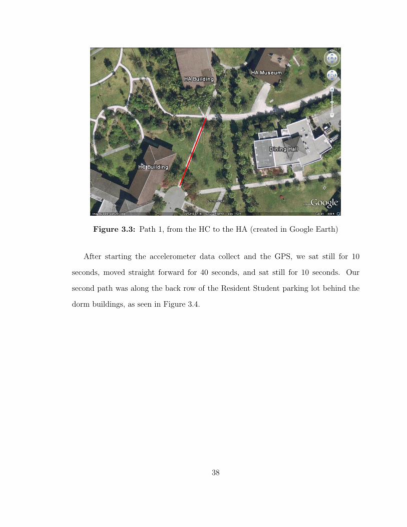
Figure 3.3: Path 1, from the HC to the HA (created in Google Earth)

After starting the accelerometer data collect and the GPS, we sat still for 10

seconds, moved straight forward for 40 seconds, and sat still for 10 seconds. Our

second path was along the back row of the Resident Student parking lot behind the

dorm buildings, as seen in Figure 3.4.

38

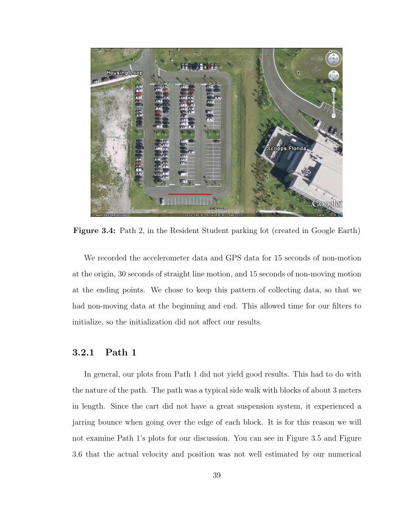
Figure 3.4: Path 2, in the Resident Student parking lot (created in Google Earth)

We recorded the accelerometer data and GPS data for 15 seconds of non-motion

at the origin, 30 seconds of straight line motion, and 15 seconds of non-moving motion

at the ending points. We chose to keep this pattern of collecting data, so that we

had non-moving data at the beginning and end. This allowed time for our filters to

initialize, so the initialization did not affect our results.

3.2.1 Path 1

In general, our plots from Path 1 did not yield good results. This had to do with

the nature of the path. The path was a typical side walk with blocks of about 3 meters

in length. Since the cart did not have a great suspension system, it experienced a

jarring bounce when going over the edge of each block. It is for this reason we will

not examine Path 1’s plots for our discussion. You can see in Figure 3.5 and Figure

3.6 that the actual velocity and position was not well estimated by our numerical

39

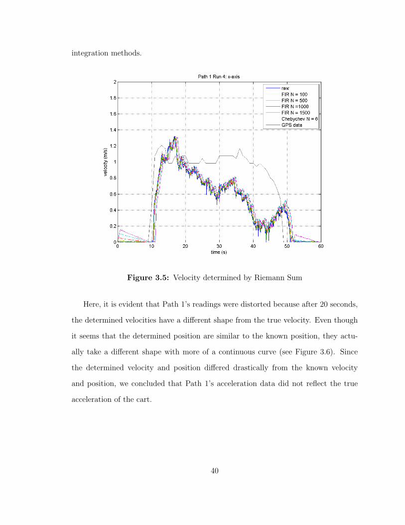
integration methods.

Figure 3.5: Velocity determined by Riemann Sum

Here, it is evident that Path 1’s readings were distorted because after 20 seconds,

the determined velocities have a different shape from the true velocity. Even though

it seems that the determined position are similar to the known position, they actu-

ally take a different shape with more of a continuous curve (see Figure 3.6). Since

the determined velocity and position differed drastically from the known velocity

and position, we concluded that Path 1’s acceleration data did not reflect the true

acceleration of the cart.

40

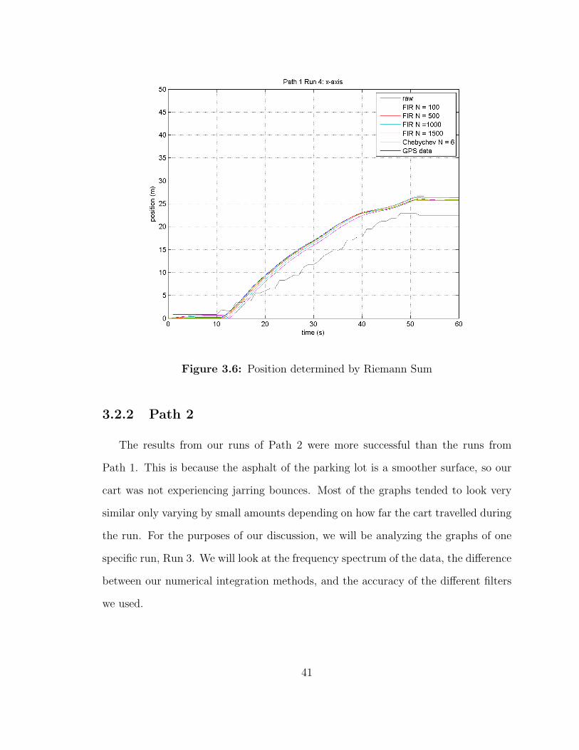
Figure 3.6: Position determined by Riemann Sum

3.2.2 Path 2

The results from our runs of Path 2 were more successful than the runs from

Path 1. This is because the asphalt of the parking lot is a smoother surface, so our

cart was not experiencing jarring bounces. Most of the graphs tended to look very

similar only varying by small amounts depending on how far the cart travelled during

the run. For the purposes of our discussion, we will be analyzing the graphs of one

specific run, Run 3. We will look at the frequency spectrum of the data, the difference

between our numerical integration methods, and the accuracy of the different filters

we used.

41

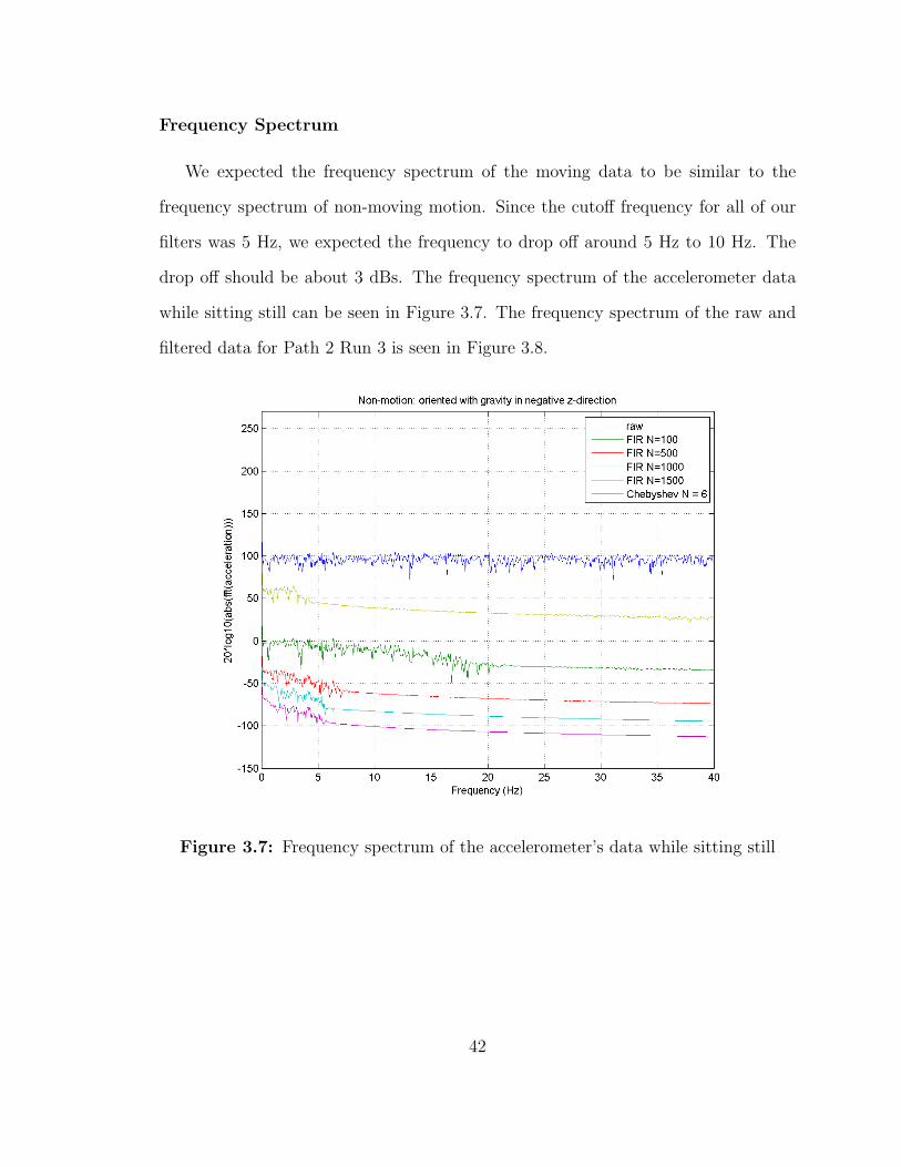
Frequency Spectrum

We expected the frequency spectrum of the moving data to be similar to the

frequency spectrum of non-moving motion. Since the cutoff frequency for all of our

filters was 5 Hz, we expected the frequency to drop off around 5 Hz to 10 Hz. The

drop off should be about 3 dBs. The frequency spectrum of the accelerometer data

while sitting still can be seen in Figure 3.7. The frequency spectrum of the raw and

filtered data for Path 2 Run 3 is seen in Figure 3.8.

Figure 3.7: Frequency spectrum of the accelerometer’s data while sitting still

42

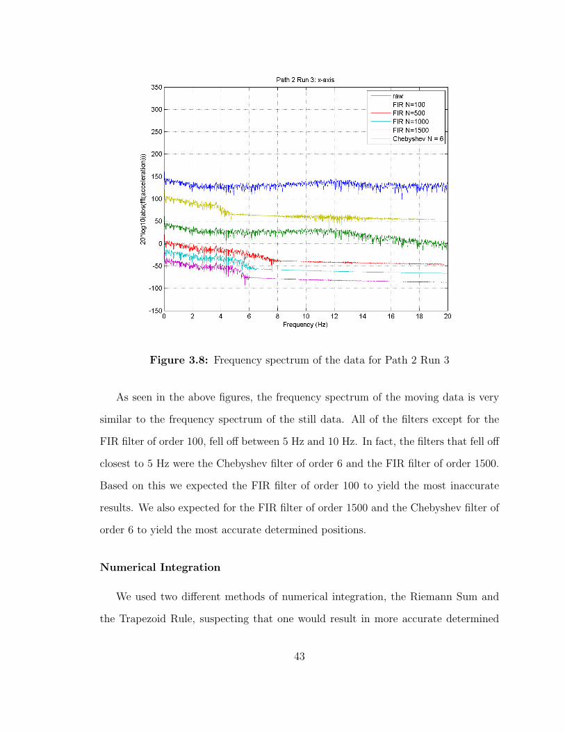
Figure 3.8: Frequency spectrum of the data for Path 2 Run 3

As seen in the above figures, the frequency spectrum of the moving data is very

similar to the frequency spectrum of the still data. All of the filters except for the

FIR filter of order 100, fell off between 5 Hz and 10 Hz. In fact, the filters that fell off

closest to 5 Hz were the Chebyshev filter of order 6 and the FIR filter of order 1500.

Based on this we expected the FIR filter of order 100 to yield the most inaccurate

results. We also expected for the FIR filter of order 1500 and the Chebyshev filter of

order 6 to yield the most accurate determined positions.

Numerical Integration

We used two different methods of numerical integration, the Riemann Sum and

the Trapezoid Rule, suspecting that one would result in more accurate determined

43

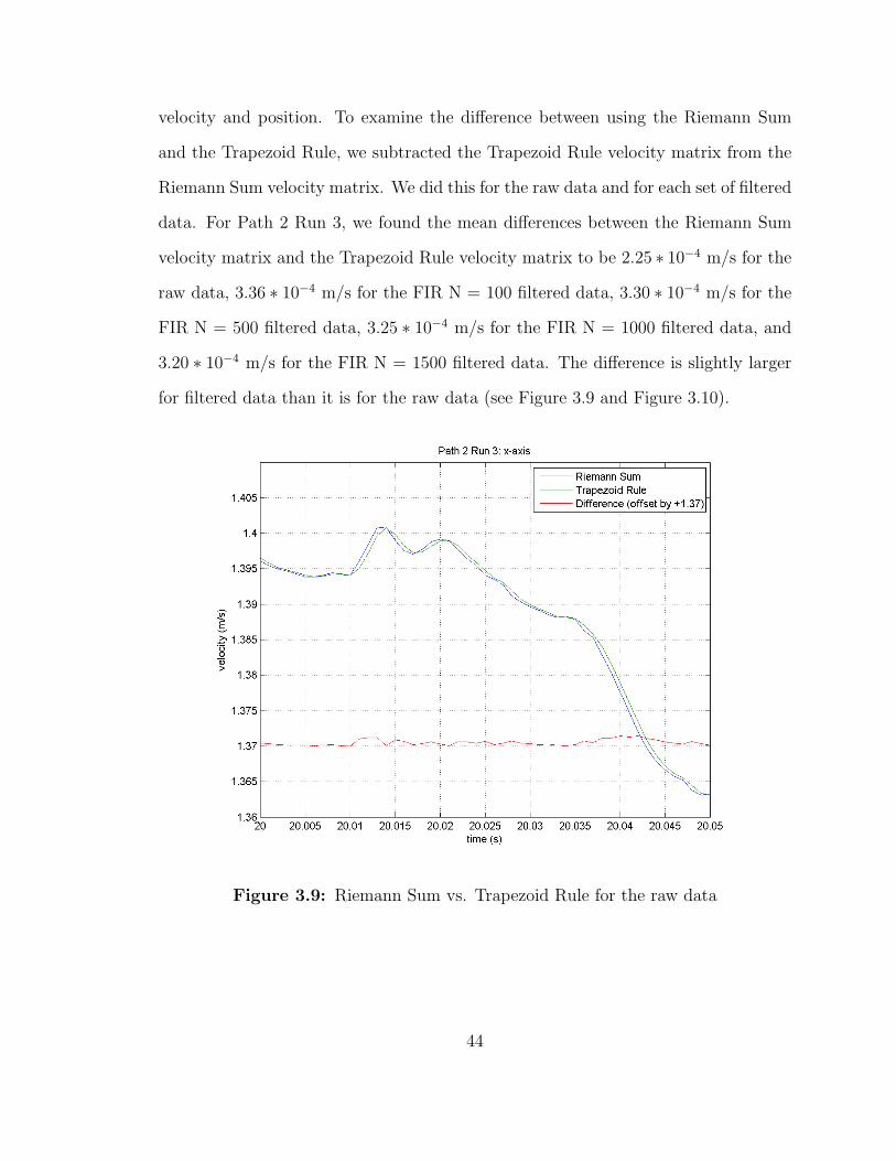
velocity and position. To examine the difference between using the Riemann Sum

and the Trapezoid Rule, we subtracted the Trapezoid Rule velocity matrix from the

Riemann Sum velocity matrix. We did this for the raw data and for each set of filtered

data. For Path 2 Run 3, we found the mean differences between the Riemann Sum

velocity matrix and the Trapezoid Rule velocity matrix to be 2.25 ∗ 10−4 m/s for the

raw data, 3.36 ∗ 10−4 m/s for the FIR N = 100 filtered data, 3.30 ∗ 10−4 m/s for the

FIR N = 500 filtered data, 3.25 ∗ 10−4 m/s for the FIR N = 1000 filtered data, and

3.20 ∗ 10−4 m/s for the FIR N = 1500 filtered data. The difference is slightly larger

for filtered data than it is for the raw data (see Figure 3.9 and Figure 3.10).

Figure 3.9: Riemann Sum vs. Trapezoid Rule for the raw data

44

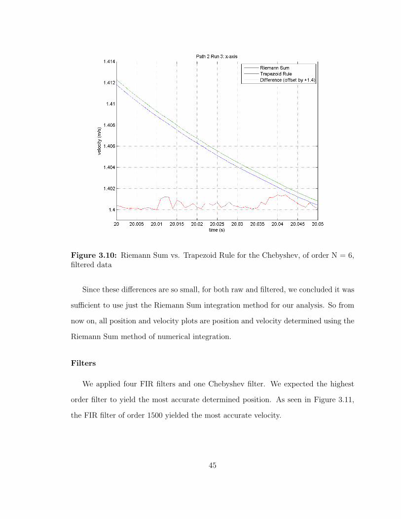
Figure 3.10: Riemann Sum vs. Trapezoid Rule for the Chebyshev, of order N = 6,filtered data

Since these differences are so small, for both raw and filtered, we concluded it was

sufficient to use just the Riemann Sum integration method for our analysis. So from

now on, all position and velocity plots are position and velocity determined using the

Riemann Sum method of numerical integration.

Filters

We applied four FIR filters and one Chebyshev filter. We expected the highest

order filter to yield the most accurate determined position. As seen in Figure 3.11,

the FIR filter of order 1500 yielded the most accurate velocity.

45

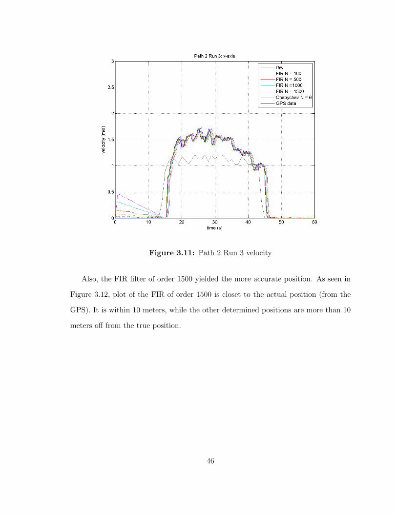
Figure 3.11: Path 2 Run 3 velocity

Also, the FIR filter of order 1500 yielded the more accurate position. As seen in

Figure 3.12, plot of the FIR of order 1500 is closet to the actual position (from the

GPS). It is within 10 meters, while the other determined positions are more than 10

meters off from the true position.

46

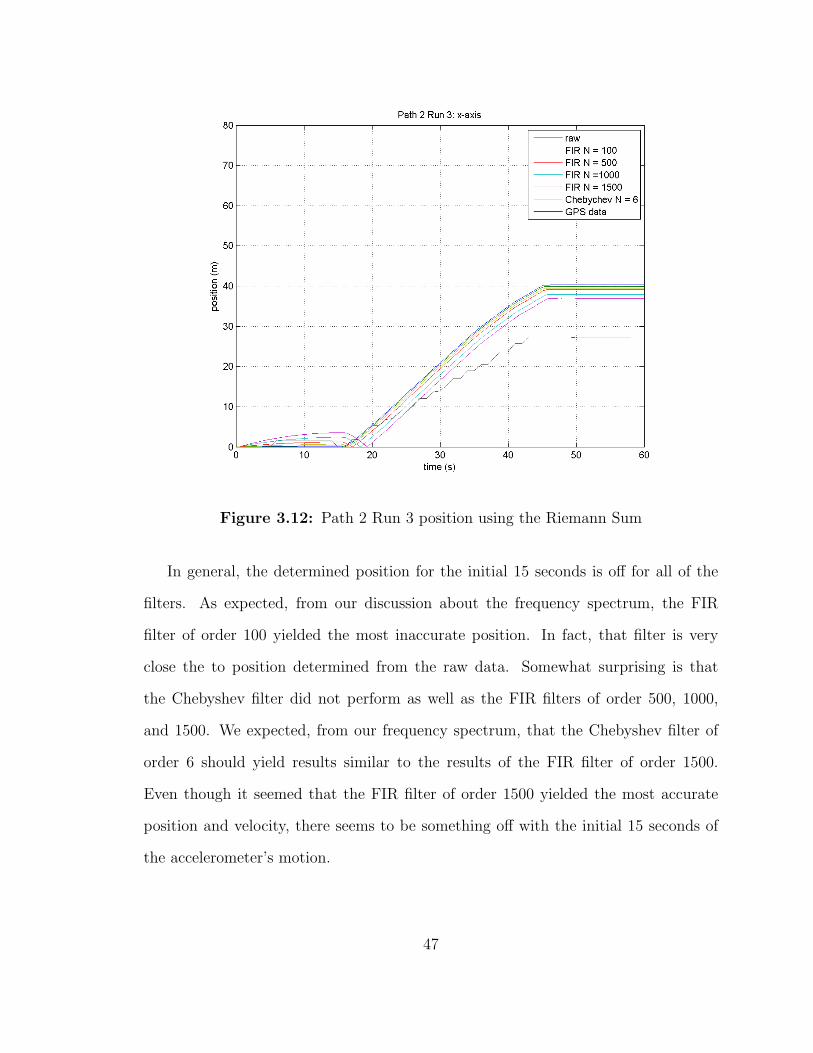
Figure 3.12: Path 2 Run 3 position using the Riemann Sum

In general, the determined position for the initial 15 seconds is off for all of the

filters. As expected, from our discussion about the frequency spectrum, the FIR

filter of order 100 yielded the most inaccurate position. In fact, that filter is very

close the to position determined from the raw data. Somewhat surprising is that

the Chebyshev filter did not perform as well as the FIR filters of order 500, 1000,

and 1500. We expected, from our frequency spectrum, that the Chebyshev filter of

order 6 should yield results similar to the results of the FIR filter of order 1500.

Even though it seemed that the FIR filter of order 1500 yielded the most accurate

position and velocity, there seems to be something off with the initial 15 seconds of

the accelerometer’s motion.

47

3.3 Discussion

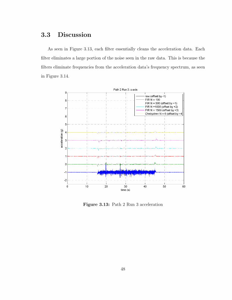
As seen in Figure 3.13, each filter essentially cleans the acceleration data. Each

filter eliminates a large portion of the noise seen in the raw data. This is because the

filters eliminate frequencies from the acceleration data’s frequency spectrum, as seen

in Figure 3.14.

Figure 3.13: Path 2 Run 3 acceleration

48

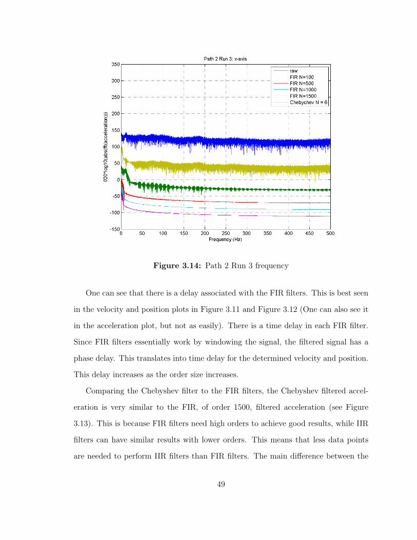
Figure 3.14: Path 2 Run 3 frequency

One can see that there is a delay associated with the FIR filters. This is best seen

in the velocity and position plots in Figure 3.11 and Figure 3.12 (One can also see it

in the acceleration plot, but not as easily). There is a time delay in each FIR filter.

Since FIR filters essentially work by windowing the signal, the filtered signal has a

phase delay. This translates into time delay for the determined velocity and position.

This delay increases as the order size increases.

Comparing the Chebyshev filter to the FIR filters, the Chebyshev filtered accel-

eration is very similar to the FIR, of order 1500, filtered acceleration (see Figure

3.13). This is because FIR filters need high orders to achieve good results, while IIR

filters can have similar results with lower orders. This means that less data points

are needed to perform IIR filters than FIR filters. The main difference between the

49

FIR filter of order 1500 and the Chebyshev filter of order 6, is that the Chebyshev

filtered data does not have the time delay that the FIR filtered data has. This is most

evident in Figure 3.11 and Figure 3.12. Even though the FIR of order 1500 filtered

acceleration data is similar to the Chebyshev of order 6 filtered data, we see that for

the velocity and position plots, for the Chebyshev filtered data is between the FIR

of order 100 and the FIR order 500. This is because the Chebyshev does not filter

out as many frequencies as the FIR filters (see Figure 3.14). Since the lower order

Chebyshev filter smoothed the acceleration data as well as the FIR of order 1500, an

IIR filter may be more appropriate as a filter for MEMS accelerometer data. In fact,

a Chebyshev filter of higher order than 6 might yield better determined velocity and

position than any of the FIR filters.

The only issue with increasing the order of the Chebyshev, is that IIR filters are

unstable. So not all orders will work well. For example, we applied a Chebyshev

filter of order 10 to see how an increasing the order by just 4 would do. The velocity

and position plots of the Chebyshev of order 10 filtered data show that the filtered

acceleration yields very inaccurate results (see Figure 3.15). The velocity and position

looks nothing like the Chebyshev of order 6 filtered acceleration. This exercise shows

that if the order of an IIR filter is too high, the filter will result in very inaccurate

measurements. Since IIR filters are sometimes unstable, and FIR filters are always

stable, FIR filters tend to be more favorable than IIR filters.

50

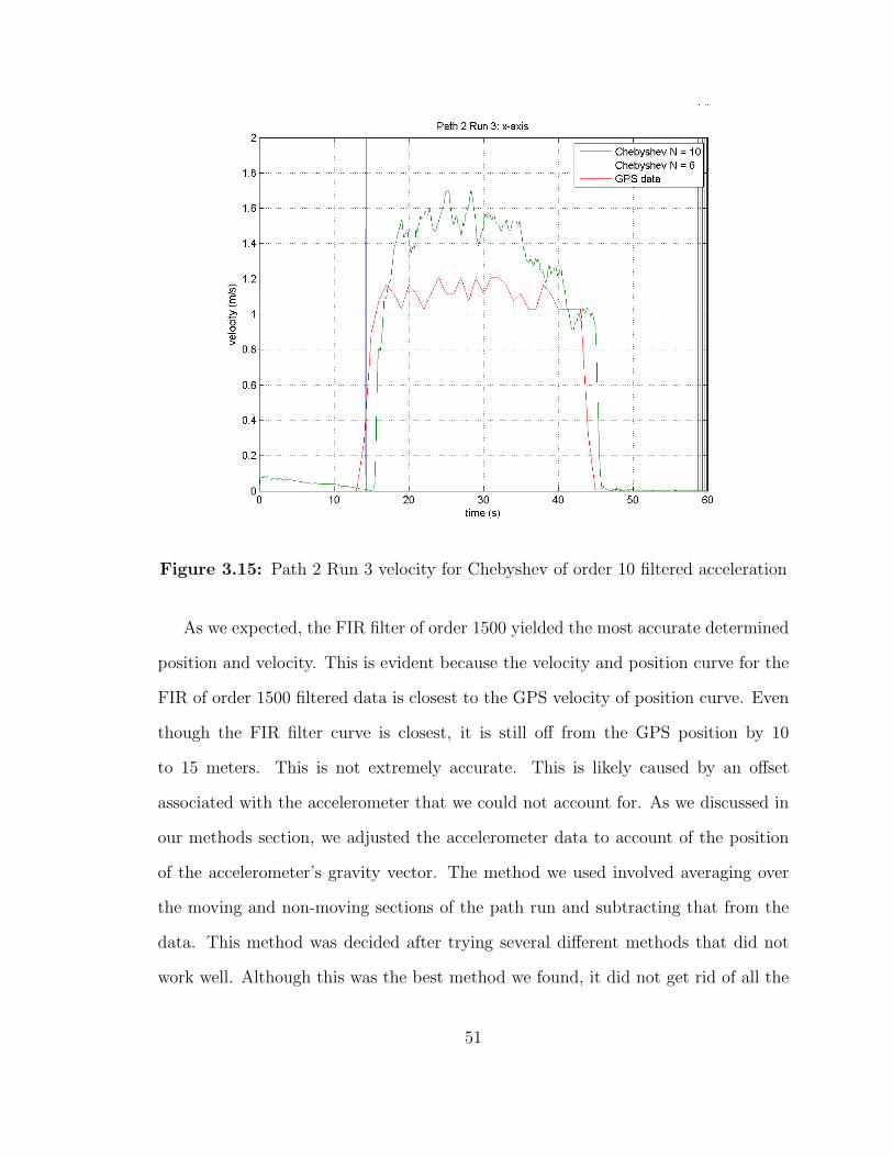
Figure 3.15: Path 2 Run 3 velocity for Chebyshev of order 10 filtered acceleration

As we expected, the FIR filter of order 1500 yielded the most accurate determined

position and velocity. This is evident because the velocity and position curve for the

FIR of order 1500 filtered data is closest to the GPS velocity of position curve. Even

though the FIR filter curve is closest, it is still off from the GPS position by 10

to 15 meters. This is not extremely accurate. This is likely caused by an offset

associated with the accelerometer that we could not account for. As we discussed in

our methods section, we adjusted the accelerometer data to account of the position

of the accelerometer’s gravity vector. The method we used involved averaging over

the moving and non-moving sections of the path run and subtracting that from the

data. This method was decided after trying several different methods that did not

work well. Although this was the best method we found, it did not get rid of all the

51

offset bias caused by the accelerometer. In Figure 3.11, all of the accelerometer data

(raw and filtered) is about 0.5 ms

larger that the GPS velocity data. This suggests

we were unable to account for all the offset bias. Had this bias been accounted for,

the determined position for both raw and filtered data would have been closer to the

GPS data. Since we cannot determine by how much the raw and filtered data would

have been improved, we cannot conclude that an FIR filter is the best filter technique

for MEMS accelerometers. Also, the time delay associated with FIR filters, suggests

that an IIR filter may be more appropriate for filtering MEMS accelerometer data.

This is because lower order IIR filters have the potential to yield accurate results

while not having a time delay in the filtered signal. We would have to try higher

order Chebyshev filters to see if they work better. This is limited because IIR filters

are unstable and higher order IIR filters may not work.

3.4 Conclusion

We examined the success of applying finite impulse response (FIR) filters and

infinite impulse response (IIR) filters to the signal from an Analog Devices’ ADXL330

iMEMS accelerometer. After converting the output voltages into acceleration, we

applied four different filters to the data: FIR filter of order N = 100, FIR filter

of order N = 500, FIR filter of order N = 1000, FIR filter of order N = 1500, and

Chebyshev (an IIR filter) of order N = 6. Firstly, we looked at the frequency spectrum

of the acceleration data. Secondly, we calculated the determined velocity and position

of the raw and filtered data. In order to determine velocity we had to integrate

the acceleration. To determine position we had to integrate velocity. Since our

signal was discrete, we had to use numerical integration methods to integrate the

signal. We applied the Riemann Sum and the Trapezoid Rule to see if either method

52

of numerical integration yielded more accurate results. Lastly, we compared the

determined velocity and position to the true velocity and position given by a handheld

GPS receiver. Overall, we looked at how filtering the signal affects the accuracy of

the determined velocity and position.

Frequency Spectrum

The frequency spectrum of the raw and filtered data looked as we suspected, the

frequency spectrum of the moving data looked very similar to the frequency spectrum

of the non-moving data (see Figure 3.7 and Figure 3.8). All of the filters removed

frequencies from the signal. The larger the order of the FIR filter, the more frequencies

were removed. Also, all of the filtered frequencies cut-off at around 5 Hz to 10 Hz

with the exception of the FIR filter of order N = 100, which cuts off around 20 Hz.

We defined the cut-off to be 5Hz for all filters, so the only two filters that cut off near

the expected frequency were the FIR filter of order 1500 and the Chebyshev filter of

order 6 (see Figure 3.8). The eliminated frequencies resulted in a cleaner (less noisy)

acceleration signal (see Figure 3.13). The higher the order of the FIR filter, the less

noisy the acceleration.

Numerical Integration

Although we expected to see a difference between using the Riemann Sum and

the Trapezoid Rule to integrate our acceleration, we found the difference was so small

that we decided to use only the Reimann Sum. We observed that the difference was

smallest for the raw data (see Figure 3.9) and increased, very slightly, for the filtered

data (see Figure 3.10). The difference between the Riemann Sum integrated velocity

and the Trapezoid Rule integrated velocity, for raw and all filtered data, was on the

53

magnitude of 10−4ms

. Thus, we used the Riemann Sum to integrate our acceleration

data to get determined velocity and position.

Filters

As we expected, the FIR of order 1500 yielded the most accurate velocity and

position. The FIR of order 1500 filtered position was within 10 to 15 meters of the

true position. Since our determined velocity was consistently 1.5 ms

more than the true

velocity, we know there was some offset bias we could not account for. This offset bias

prevented us for getting a more precise comparison between the determined position

of the filtered data and the true position. That is why our FIR of order 1500 filtered

data did not yield a determined position closer to the true position.

We also examined the success of applying FIR filters versus IIR filters. There is

a time delay in FIR filtered signals that is most evident in the velocity and position

plots (see Figure 3.11 and Figure 3.12). This time delay occurs because there is a

phase delay associated with FIR filters. This time delay increases as the order of the

FIR filter increases. IIR filters do not have a phase delay, so there is not a time delay

in the Chebyshev filtered signals. Since we do not want a time delay, an IIR filter

may be more appropriate. Also, while FIR filters require large orders to work well,

IIR filters do not. This is why the FIR of order 1500 filtered acceleration signal is

similar to the Chebyshev of order 6 filtered acceleration (see Figure 3.13). The issue

with using an IIR filter is that they are unstable, thus higher order IIR filters can

yield very distorted signals. We showed this by applying a Chebyshev filter of order

10 to our acceleration data (see Figure 3.15). This makes it hard to increase the order

of an IIR filter with the hope of getting more accurate results.

Overall, our FIR filters were more robust than our IIR filters. Despite the phase

54

delay large orders needed, our FIR filters were successful because they are always

stable. In fact, our FIR filter of order 1500 had the most accurate position results.

IIR filters do have potential because they lack a phase delay and require small orders,

but they are inherently unstable. This makes FIR filters more robust than IIR filters.

Although the offset bias associated with our accelerometer did not allow us to

precisely compare determined velocity and position with known velocity and position,

we were still able to examine the issues associated with both FIR and IIR filters. We

showed that our highest order FIR filter (n = 1500) was our most robust filter and

yielded the most accurate results (position off by about 10 to 15 meters). This

accuracy was also limited by the time delay in the velocity and position created by

applying the FIR filter. Since the IIR filter requires low orders and lacks the time

delay, an IIR filter may be better for this application. The issue with applying an IIR

filter is that IIR filters are unstable and high order IIR filters can result in distorted

signals. Thus, even though IIR filters lack a time delay and require low orders, their

unstable nature makes them difficult to use. That is why FIR filters, which are always

stable, are good choices for filtering data. Overall, this thesis provided insight into the

use of FIR filters and IIR filters as a means to eliminate noise in MEMS accelerometer

data.

This study can be expanded to examine the effect of using FIR and IIR filters on

the signals from MEMS motion sensors. This experiment can be redone including a

variety of MEMS accelerometers or a variety of MEMS gyroscopes. It can even be

redone with both MEMS accelerometers and MEMS gyroscopes as a way to simulate

a MEMS-based Inertial Measurement Unit. Also, we could use different designs of

the same filters used in this study. We could look at different cutoff frequencies and

different orders for both FIR and IIR filters. This way the potential of using an IIR

filter could be better determined. This study could also be altered to investigate the

55

effects of other type of digital filters. It could be repeated using different types of FIR

and IIR filters. Also, it can be redone with different filters such as the Kalman filter.

The overall goal of this study, and similar studies, is to design a filtering technique

that yields accurate enough position and velocity signals to be used in a MEMS-

based Inertial Measurement Unit. This is done by inspecting the successes and issues

of various digital filters when they are applied to MEMS motion sensors.

56

Bibliography

[1] Baoping Xiao, Change Xu, and Lijun Xu. An application of MEMS sensors in

inertial navigation system. pages 360–363, 2009.

[2] Aboelmagd Noureldin, Tasfen B. karamat, Mark D. Eberts, and Ahmed El-

Shafie. Performance enhancement of MEMS-based INS/GPS integration for

low-cost navigation applications. IEEE Transaction on Vehicular Technology,

58(3):1077–1096, March 2009.

[3] N. M. Faulkner, S. J. Cooper, and P.A. Jeary. Integrated MEMS/GPS naviga-

tions systems. Institute of Electrical and Electronics Engineers, pages 306–313,

2002.

[4] Yung-Yue Chen, Shyang-Jye Chang, and Ren-Yuan Yu. Robust estimation de-

sign of MEMS-based integration inertial navigation. Institue of Electrical and

Electronics Engineers, pages 3117–3122, 2006.

[5] Sergio Baselga, Luis Garcia-Asenjo, Pascual Garrigues, and Jose Luis Lerma.

Inertial navigation system data filtering prior to GPS/INS integration. The

Journal of Navigation, pages 711–720, 2009.

[6] Paul L. Bergstrom, Melissa L. Trombley, and Gary G. Li. MEMS: Application,

chapter 2: Inertial Sensors. CRC Press Taylor and Francis Group, Boca Raton

FL, 2nd edition, 2006.

[7] Ferdinand P. Beer, E. Russell Johnston Jr., and Philip J. Cornwell. Vector

Mechanics for Engineers: Dynamics. McGraw-Hill Higher Education, 2010.

57

[8] Wikimedia, October 2009. http://commons.wikimedia.org/wiki/File:3D_

Gyroscope-no_text.png.

[9] Nadim Maluf and Kirt Williams. Introduction to Microelectromechanical Systems

Engineering. Artech House Inc., Boston MA, 2nd edition, 2004.

[10] James J. Allen. MicroElectroMechanical System Design. CRC Press Taylor and

Francis Group, Boca Raton FL, 2005.

[11] Device Basics: Mircoelectromechanical Systems. Semiconductor International,

June 2003. Vol. 26, Issue 6, 128.

[12] Mircoelectromechanical systems: Advanced materials and fabrication methods.

National Academies Press, 1997. Washington DC.

[13] Ashok Ambardar. Analog and Digital Signal Processing. PWS Publishing Com-

pany, Boston, MA, 1995.

[14] Ralph D. Hippenstiel. Detection Theory: Applications and Digital Signal Pro-

cessing. CRC Pres, Boca Raton, FL, 2002.

[15] Calculus: Multivariable. John Wiley and Sons Inc., 2005.

[16] Wikimedia, November 2005. http://upload.wikimedia.org/wikipedia/

commons/8/82/Riemann-Sum-right-hand.png.

58