Embed Size (px)
Citation preview

Reference Readings & Homework Exercises for
Discrete Difference Equations
Written by
Prof. Erin N. Bodine
Prepared for
Math 214: Discrete Math Modeling (Fall 2014)
Rhodes College

Discrete Difference Equations 1
1 An Introduction to Discrete Mathematical Modeling
The field of mathematics provides many different means for modeling the world around us. Some mathematical tools
are more appropriate for modeling certain phenomenon and less appropriate for other phenomenon. In this course we
focus on how to use mathematics to simulate biological situations in which it is reasonable to assume the underlying
variable of the model is discrete, that is, it can be written as a sequence of values. In contrast, the real number line
is continuous and for any two values a and b (no matter how close a and b are on the number line), we can always
find another value that is between a and b. We may have to increase our precision to achieve this, but it can always
be done. A sequence of discrete values is a set of points along the real number line. Thus, with a discrete model, we
are assuming that we can ignore the space between the points.
As one example, suppose we grow a cell culture in petri dish and measure the cell density (cells per unit area)
every hour for 24 hours. This would create a sequence of 25 data points (if we include the initial cell density). We
know that the cell culture is growing during the time between when we take our measurements, but measuring the
population each hour over the course of a day will give us a reasonable representation of how the culture grows over
the course of one day. Correspondingly, when we build a mathematical model to represent the growth of the cell
culture, it is reasonable for the model to only predict how the culture grows from hour to hour. Thus, the underlying
variable, time, is represented in the mathematical model as increasing in discrete, one hour increments.
For another example, consider a population which breeds seasonally, that is, only once a year. If we wanted to
determine how the population size is changing over the course of many years, we could collect data to estimate the
size of the population at the same time each year (say shortly after the breeding season ends). We know that between
the times at which we estimate the population size some individuals will die and during the breeding season many
new individuals will be born, however, we ignore the changes in population size from day to day, or week to week, and
look only at how the population size changes from year to year. Thus, when we build a mathematical model of this
population, it is reasonable for the model to only predict the population size for each year shortly after the breeding
season. Here, the underlying variable, time, is represented in the mathematical model as increasing in discrete, one
year increments.
2 A Motivating Example: Cell Growth
Let us consider an actual data set for the cell growth example described above. The data in Table 1 give the optical
density of an Escherichia coli (commonly referred to as E. coli) cell culture measured every 30 minutes for 3 hours.
The culture was grown in a nutrient solution at 37◦C.
Table 1: Optical Density of E. coli cell culture.
Time (hours) 0.0 0.5 1.0 1.5 2.0 2.5 3.0
Cell Density (OD600) 0.055 0.120 0.231 0.360 0.516 0.821 1.300

Discrete Difference Equations 2
Escherichia coli : Abbreviated as E. coli, this bacteria lives in the lower intestines of endotherms (warm bloodedorganisms), including humans. There are variety of strains of E. coli many of which are part of the natural microbiomeof an endotherm’s intestinal tract. However, there are some strains of E. coli which can cause severe and adversereactions in their hosts including vomiting, fever, aches, and diarrhea (in humans).
Figure 1: Optical density of the E. coli cell culture measured every30 minutes over 3 hours.
If we plot the data in Table 1 we obtain the graph in Fig-
ure 1. When we examine this data it would appear that
the cell density is growing exponentially. How might we
approximate this sequence of cell densities using an alge-
braic expression, that is, a mathematical model?
In general, when we want to describe a sequence mathe-
matically, we want to express how the (n+ 1)th term in
the sequence, xn+1 is determined using previous n terms
in the sequence, xn, xn−1, xn−2, . . . , x1, x0. Mathe-
matically, we express the term xn+1 as a function of the
previous n terms, that is
xn+1 = f(xn, xn−1, xn−2, . . . , x1, x0). (1)
Table 2: Differences & ratios of consecutive terms of Sequence (2).
n xn+1 − xn xn+1/xn
0 0.065 2.18
1 0.111 1.93
2 0.129 1.56
3 0.156 1.43
4 0.305 1.59
5 0.479 1.58
Equations which can be expressed in the form of Equa-
tion (1) are known as discrete difference equa-
tions.
For simplicity, let us assume that the next value in the
cell density sequence can be determined using only the
previous value in the sequence. Thus, xn+1 is a func-
tion of xn, that is xn+1 = f (xn), which is called a first
order difference equation . Often we can determine
the relationship between two consecutive terms in a se-
quence, xn and xn+1, by examining either the difference or ratio between those two terms, that is xn+1 − xn or
xn+1/xn, respectively. For the data presented in Table 1, let xn represent the cell density of the nth data point,
where n = 0 denotes the data point at 0 hours, n = 1 denotes the data point at 30 minutes, etc. Thus,
x0 = 0.055, x1 = 0.120, x2 = 0.231, x3 = 0.360, x4 = 0.561, x5 = 0.821, x6 = 1.300, (2)
where the underlying variable, time, is represented as increasing in discrete 30 minute increments. Table 2 shows
both the difference and ratio of consecutive terms in the sequence representing the cell density data from Table 1.
The difference between consecutive terms in the sequence are increasing as n increases. However, with the exception
of the first two ratios, the ratios of consecutive terms appears to remain relatively constant as n increases. Suppose
the ratios of consecutive terms were constant with a value c as n increased, then
xn+1
xn= c ⇒ xn+1 = cxn,

Discrete Difference Equations 3
and thus we have written xn+1 as a function of xn (where f(xn) = cxn). Given that the ratios of consecutive terms
show little fluctuation, we might assume that the fluctuations we see are due to measurement error (either by the
spectrophotometer used to measure the optical density or by the human taking the measurements). If we assume
that the ratios of consecutive terms would be constant if not for measurement error, then what would be the value
of c? We could use the average (mean value) of all of the ratios: 1.7. We could also use the average of the last four
ratios: 1.5. Thus, we have two options for our model:
xn+1 = 1.7xn (model 1), and xn+1 = 1.5xn (model 2).
Figure 2: Optical density of the E. coli cell culture measured every30 minutes over 3 hours (dotted grey), and estimated optical densityusing model 1 (solid blue) and model 2 (dashed red).
How do we decide which model is “better”? First, what
does it mean for one model to be better than another
model? In this case, we are interested in seeing which
model is better able to accurately reproduce the data.
When we use model 1 with x0 = 0.055, we generate the
sequence
x0 = 0.055, x1 = 0.094, x2 = 0.159, x3 = 0.270,
x4 = 0.459, x5 = 0.781, x6 = 1.328. (3)
When we use model 2 with x0 = 0.055, we generate the
sequence
x0 = 0.055, x1 = 0.083, x2 = 0.124, x3 = 0.186,
x4 = 0.278, x5 = 0.418, x6 = 0.626. (4)
Figure 2 show a plot of the sequence of the original data (gray) against the sequences generated by model 1 (blue)
and model 2 (red). Which model appears to approximate the data better? It would appear that model 1, though
not perfect, does a better job approximating the data.
Optical Density: How does one “count” the number of cells in a cell culture? The number of cells in a culture couldbe quite large (on the order of millions or billions). It would indeed be a tedious task to sit down and count the totalnumber of cells in such a culture. In fact, if the culture is growing (the number of cells are increasing), by the timeyou counted the first 200 cells, the size of culture would likely have changed. Instead of counting the number of cellsin a culture of volume V , we sample the culture, that is, we take a representative portion of the culture and countthe number of cells in the sample. Suppose the sample has Ns cells, and a volume of Vs. If we assume that the celldensity (cells per unit volume) are the same in the whole culture as in the sample, then N/V = Ns/Vs, where N is thetotal number of cells in the sample. Thus, N = V (Ns/Vs). The ratio Ns/Vs is proportional to the optical density (i.e.Ns/Vs = a ·OD where a is a constant and OD is the optical density) and is measured using a spectrophotometer. Thesample is placed in a cuvette (essentially a rectangular test tube) and the spectrophotometer shines a beam of light (ofa specified wavelength) through the cuvette. The denser the cell culture, the less light will shine through the cuvette.By measuring the amount of light that does not make it through the cuvette (light that scatters due to the cells inthe cuvette), the spectrophotometer measures the optical density of the cell culture sample. The intensity of the lightscattering, and thus the measure of optical density, depends on the wavelength of light being used. The wavelengthof light used, measured in nanometers (nm), is denoted by a subscript of OD. Thus, an optical density measure takenusing a light with wavelength 600 nm is indicated by OD600.
Discrete Difference Equations 4
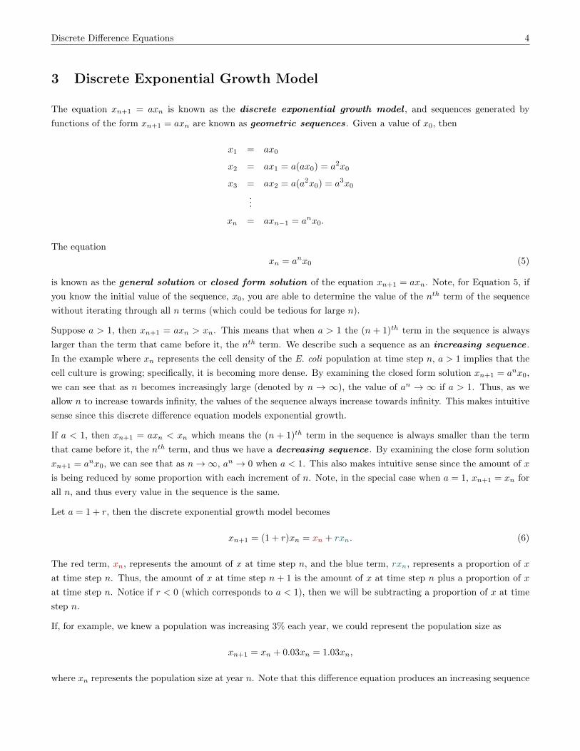
3 Discrete Exponential Growth Model
The equation xn+1 = axn is known as the discrete exponential growth model , and sequences generated by
functions of the form xn+1 = axn are known as geometric sequences. Given a value of x0, then
x1 = ax0
x2 = ax1 = a(ax0) = a2x0
x3 = ax2 = a(a2x0) = a3x0...
xn = axn−1 = anx0.
The equation
xn = anx0 (5)
is known as the general solution or closed form solution of the equation xn+1 = axn. Note, for Equation 5, if
you know the initial value of the sequence, x0, you are able to determine the value of the nth term of the sequence
without iterating through all n terms (which could be tedious for large n).
Suppose a > 1, then xn+1 = axn > xn. This means that when a > 1 the (n + 1)th term in the sequence is always
larger than the term that came before it, the nth term. We describe such a sequence as an increasing sequence .
In the example where xn represents the cell density of the E. coli population at time step n, a > 1 implies that the
cell culture is growing; specifically, it is becoming more dense. By examining the closed form solution xn+1 = anx0,
we can see that as n becomes increasingly large (denoted by n → ∞), the value of an → ∞ if a > 1. Thus, as we
allow n to increase towards infinity, the values of the sequence always increase towards infinity. This makes intuitive
sense since this discrete difference equation models exponential growth.
If a < 1, then xn+1 = axn < xn which means the (n + 1)th term in the sequence is always smaller than the term
that came before it, the nth term, and thus we have a decreasing sequence . By examining the close form solution
xn+1 = anx0, we can see that as n→∞, an → 0 when a < 1. This also makes intuitive sense since the amount of x
is being reduced by some proportion with each increment of n. Note, in the special case when a = 1, xn+1 = xn for
all n, and thus every value in the sequence is the same.
Let a = 1 + r, then the discrete exponential growth model becomes
xn+1 = (1 + r)xn = xn + rxn. (6)
The red term, xn, represents the amount of x at time step n, and the blue term, rxn, represents a proportion of x
at time step n. Thus, the amount of x at time step n + 1 is the amount of x at time step n plus a proportion of x
at time step n. Notice if r < 0 (which corresponds to a < 1), then we will be subtracting a proportion of x at time
step n.
If, for example, we knew a population was increasing 3% each year, we could represent the population size as
xn+1 = xn + 0.03xn = 1.03xn,
where xn represents the population size at year n. Note that this difference equation produces an increasing sequence

Discrete Difference Equations 5
and thus, xn →∞ as n→∞. If, on the other hand, the population was decreasing by 3% each year, then we would
represent the population size as
xn+1 = xn − 0.03xn = 0.97xn,
where xn represents the population size at year n. This difference equation produces a decreasing sequence and thus,
xn → 0 as n→∞.
Table 3: Difference quotients of consec-utive terms of Sequence (2).
n (xn+1 − xn) /xn
0 1.182
1 0.925
2 0.558
3 0.433
4 0.591
5 0.583
Note that Equation (6) can be rewritten as
xn+1 − xn = rxn, (7)
which denotes the difference in the amount of x from time n to time n + 1.
The equation in this form reveals why we refer to these types of equations as
difference equations. Note, the change in x over one time step is a proportion
(r) of the amount at the previous time step (xn). Thus, we say “the change is
x is proportional to the amount of x.” Furthermore, if we rewrite Equation (7)
asxn+1 − xn
xn= r, (8)
then we have a direct way to estimate the value of r for a model. Table 3 shows the values of the difference quotients
in Equation (8) for n = 0, 1, . . . , 5. If we average the values in the second column of Table 3, we obtain 0.619 ≈ 0.7
as an estimate of r. Note, this concurs with the value of a = 1.7 since a = 1 + r.
Example 1.We determined that a reasonable model for the density of E. coli cells given the data presented in Table 1 is
xn+1 = 1.7xn.
(a) Find the general solution to this difference equation.
(b) Does this difference equation model produce an increasing or decreasing sequence?
(c) Given this model, what cell density would we predict at 6 hours? at 10 hours? at 24 hours? Do these values make biological sense?
(d) What happens to the population of E. coli cells as n→∞? Is this biologically reasonable?
The solutions to this example will be worked in class.
Example 2.The Forest and Wildlife Research Center at Mississippi State University measured the survival and mortality rates of bobcats (Lynx
rufus) in and near the Tallahala Wildlife Management Area through their Carnivore Ecology Research Project [8]. They studied 68
bobcats (28 males and 40 females) and found that the mean annual survival was 75% for males and 84% for females.
(a) Use a discrete difference equation model to express how many male bobcats (of the original 28) are still alive at year n. Assume that
there are 28 male bobcats at year n = 0. Express the model in closed form solution.
(b) Use a discrete difference equation model to express how many female bobcats (of the original 40) are still alive at year n. Assume
that there are 40 female bobcats are year n = 0. Express the model in closed form solution.
(c) Both models generate decreasing sequences. Which is decreasing more quickly?
(d) What is the first year in which there will be no male bobcats left (i.e. less than 1 male bobcat) of the original 28? What is the first
year in which there will be no female bobcats left of the original 40?
The solutions to this example will be worked in class.

Discrete Difference Equations 6
Exercise 1 – Wild Hares
Suppose a population of wild hares increases by 12% each year, and there are currently 200 hares. Let xn be the number of hares in the
population at year n.
(a) Find the difference equation representing xn+1 as a function of xn.
(b) Find the general solution to the difference equation found in (a).
(c) Find the number of hares in the population 6 years from now.
(d) What happens to the population of hares as n→∞? Is this biologically reasonable?
Exercise 2 – Elk Herd
Let xn be the number of adult elk in a newly introduced elk herd in a wildlife management area in the Cumberland Mountains in
Tennesseee. There are currently 50 adult elk in the population.
(a) Suppose the number of adults in the population increases by 10% each year. Use a discrete difference equation model to express how
the number of adult elk in the population at year n (express your model in the closed form solution). Does your model generate an
increasing or decreasing sequence? Determine how many adult elk are in the population after 20 years.
(b) Suppose that the probability that an adult elk survives in a given year is 90%. Use a discrete difference equation model to express
how many of the originally introduced adult still alive at year n (express your model in the close form solution). Does your model
generate an increasing or decreasing sequence? Determine how many of the originally introduced elk are still alive after 20 years.
Elk live, on average, 15 years in the wild. Does your answer make biological sense?
Exercise 3 – Treating Heart Disease
Digoxin is used in the treatment of heart disease. Doctors must prescribe an amount of medicine that keeps the concentration of digoxin in
the bloodstream above a minimum level of effectiveness without exceeding the maximum level for safety (these levels vary among patients).
For an initial dosage of 0.5 mg in the bloodstream, the table below shows the amount of digoxin (x) remaining in the bloodstream of a
particular patient after n days.
Time (days) 0 1 2 3 4 5 6 7 8
Digoxin (mg) 0.500 0.345 0.238 0.164 0.113 0.078 0.054 0.037 0.026
(a) Suppose the amount of digoxin in the bloodstream of the patient can be modeled using xn+1 = axn, where xn is the amount of
digoxin (in mg) in the bloodstream on day n. Use the ratio of consecutive terms in the sequence to determine the value of a.
(b) Express your model in its closed form solution.
(c) In this patient the digoxin is effective if it remains above 0.01 mg, however digoxin toxicity occurs when the amount of digoxin in
the bloodstream exceeds 0.6 mg. When would you recommend this patient take his or her next dose of digoxin.
Note, we will revisit this example and the idea of timing between doses once we have explored some more sophisticated difference
equation models.

Discrete Difference Equations 7
4 Discrete Model with Exponential & Constant Growth
In the discrete exponential growth model, the change in x (represented as xn+1 − xn) was proportional to x (that is
xn), thus we had the equation
xn+1 − xn = rxn,
where r is the proportionality constant which represents the rate of change. However, what if the change is not
proportional, but constant, that is what if
xn+1 − xn = b, (9)
where b is a constant. Equation (9) can be rewritten as
xn+1 = xn + b, (10)
and we will refer to this model as the constant growth model . The sequence generated by Equation (10) is known
as an arithmetic sequence . As with the discrete exponential growth model, we can find a closed form solution of
the constant growth model. Given a value for x0, then
x1 = x0 + b
x2 = x1 + b = (x0 + b) + b = x0 + 2b
x3 = x2 + b = (x0 + 2b) + b = x0 + 3b
...
xn = x0 + nb.
Note, if b > 0 then the values of xn increase as n → ∞, but if b < 0 then the value of xn decrease as n → ∞. In
particular, the values of xn can become negative if b < 0 and n is large enough, even if x0 > 0. This may or may not
be biologically reasonable depending on what is being modeled.
In general, we will not use the constant growth model on its own, but in combination with the exponential growth
model. In this section we will examine a variety of models (known as first order linear difference equations) of
the form
xn+1 = axn︸︷︷︸exponential
growth
+ b︸︷︷︸constantgrowth
. (11)
Before we look at specific biological phenomenon which can be modeled using Equation (11), we shall derive the
closed form solution (see below) and discuss the notion of the model begin at equilibrium and how to determine the
long term behavior of a model (see the next section). Given x0, then the closed form solution is derived as
x1 = ax0 + b
x2 = ax1 + b = a [ax0 + b] + b = a2x0 + (a+ 1)b
x3 = ax2 + b = a[a2x0 + (a+ 1)b
]= a3x0 +
(a2 + a+ 1
)b
...
xn = anx0 +(an−1 + · · ·+ a2 + a+ 1
)b.
Discrete Difference Equations 8
This is a way to express the closed form solution, but it seems rather unwieldy. It would be nice if that (n − 1)th
order polynomial in terms of a weren’t mucking up the equation. With some good old fashioned polynomial long
division (think back to your fondest memories of Algebra II), it can be shown that
1− an = (1− a)(1 + a+ a2 + · · ·+ an−1
)⇒ 1− an
1− a= 1 + a+ a2 + · · ·+ an−1,
provided a 6= 1. Thus, we can rewrite the closed form solution as
xn = anx0 +1− an
1− ab,
which feels much more manageable as an equation, and will be easier to work with as we progress forward. Notice
if a = 1, then Equation (11) reduces to the constant growth model represented by Equation (10).
5 Equilibria & Long-Term Behavior
Equilibria
The term equilibrium refers to being in a state of balance and remaining as you are. In the case of discrete difference
equation models, a number x∗ is called an equilbrium point or fixed point of the difference equation xn+1 = f(xn)
if x∗ = f(x∗). Let us examine this concept for the few discrete difference equation models we have encountered so
far.
Exponential Growth Model · Recall the exponential growth model has the form xn+1 = axn, where a is a
constant. The model will be in equilibrium when x∗ = ax∗ which can only occur if a = 1. Thus, when a 6= 1, there
is no fixed point for the model which makes sense because the values of xn are either always increasing (a > 1) or
always decreasing (a < 1). When a = 1, xn = x0 for all n.
Constant Growth Model · Recall the constant growth model has the form xn+1 = xn+b, where b is a constant.
The model will be in equilibrium when x∗ = x∗ + b which can only occur if b = 0. Thus, when b 6= 0, there is no
fixed point for the model which make sense because the values of xn are either always increasing (b > 0) or always
decreasing (b < 0). When b = 0, xn = x0 for all n.
Exponential & Constant Growth Model · Recall the difference equation model with exponential and
constant growth has the form xn+1 = axn + b, where a and b are constants. The model will be in equilibrium
when
x∗ = ax∗ + b ⇒ (1− a)x∗ = b ⇒ x∗ =b
1− a.
This is different from the previous two examples because this does not require that a and b take on certain values
for the model to have a fixed point, and the fixed point is not necessarily the initial condition x0. When we examine
this model as it pertains to different biological phenomenon, we will see the different ways in which we can interpret
the meaning of the equilibrium value x∗.

Discrete Difference Equations 9
Long-Term Behavior
When you are examining the features of a model xn+1 = f(xn), it if often useful to know what happens to the model
as n→∞. This is known as the long-term behavior of the model. We already examined the long term behavior
of the exponential growth model and constant growth model under various parameter scenarios (a > 1, a = 1, a < 1
for the exponential growth model, and b > 0, b = 0, b < 0 for the constant growth model).
It turns out there is another, more visual way to examine the long-term behavior of these models called cobweb
diagram analysis. On the xn, xn+1 plane (where xn is the horizontal axis and xn+1 is the vertical axis), we plot
xn+1 = f(xn) and xn+1 = xn. On the xn (horizontal) axis, locate x0. Draw a vertical line from x0 on the horizontal
axis to the xn+1 = f(xn) curve. Your height on the vertical axis now represents x1. To locate x1 on the horizontal
axis, draw a horizontal line from (x0, x1) to the xn+1 = xn line; you are now at (x1, x1). Then, (starting with
n = 1)
1. Draw a vertical line from (xn, xn) to the curve xn+1 = f(xn); you are now at (xn, xn+1).
2. Draw a horizontal line from (xn, xn+1) to the line xn+1 = xn; you are now at (xn+1, xn+1).
3. Repeat steps 1 & 2 with increasing values of n as many times as needed to see a pattern.
Figure 3 shows what this looks like for the discrete exponential growth model when (a) a > 1 and (b) a < 1. In
each graph the blue curve represents xn+1 = axn and the black line represents xn+1 = xn. The dotted red line show
the “cobwebbing”. In Figure 3a (where a > 1) we can see that the cobwebbing (dotted red line) steps up and away
from x0 as n increases. This is because the values of xn (and thus xn+1) are increasing as n increases. In Figure 3b
(where 0 < a < 1) we can see that the cobwebbing (dotted red line) steps down towards (0, 0) as n increases.
This method may seem like overkill for these simple difference equations but it will be very handy for analyzing the
long-term behavior of xn+1 = axn + b.
(a) a > 1 (b) a < 1
Figure 3: Cobweb diagrams for the discrete exponential growth model for (a) a > 1 and (b) a < 1.
Note that for the difference equation model with exponential and constant growth, xn+1 = axn + b, it is a little
harder to determine the long term behavior because their are two parameters, a and b, and the relative size and sign
of each parameter will have a bearing on what happens to the values of xn as n→∞. Suppose x0 > 0. If a > 1 and
b > 0 we would expect the population to grow, and if a < 1 and b < 0 we would expect the population to decline.

Discrete Difference Equations 10
And indeed, in both cases we are correct as shown in the cobweb diagrams depicted in Figures 4a and 4b. Notice
that in the case where a < 1 and b < 0, the values of xn quickly become negative despite the fact that x0 > 0.
(a) a > 1, b > 0 (b) a < 1, b < 0
(c) a < 1, b > 0 (d) a > 1, b < 0
Figure 4: Cobweb diagrams for xn+1 = axn + b.
Now, suppose a < 1 and b > 0. What do we expect to happen in this case. The value of a will cause a decrease
while the value of b will cause an increase. If we examine the cobweb diagram in Figure 4c we see that the lines
xn+1 = xn and xn+1 = axn + b cross in the first quadrant at the point(
b1−a ,
b1−a
). Notice if we choose x0 = b
1−a ,
then xn = b1−a for all n, and thus x∗ = b
1−a is an equilibrium point. If we choose x0 such that 0 < x0 <b
1−a , then
the values of xn increase towards b1−a . If we choose x0 >
b1−a , then the values of xn decrease towards b
1−a . Thus, no
matter what value of x0 we choose, as n→∞ the values of xn approach b1−a . Since the sequence of values approach
the equilibrium point, we classify the fixed point as a stable equilibrium .
Lastly, suppose a > 1 and b < 0. If we examine the cobweb diagram in Figure 4d we see again that the lines
xn+1 = xn and xn+1 = axn + b cross in the first quadrant at the point(
b1−a ,
b1−a
), and that if we choose x0 = b
1−a ,
then xn = b1−a for all n, and thus x∗ = b
1−a is an equilibrium point. However, if we choose x0 such that 0 < x0 <b
1−a ,
then the values of xn decrease towards −∞. If we choose x0 >b
1−a , then the values of xn increase towards ∞. In
this case, not matter what value of x0 we choose, with the exception of x0 = b1−a , as n→∞ the values of xn move
away from b1−a , and we classify this type of fix point as an unstable equilibrium .

Discrete Difference Equations 11
Example 3.Consider a lake fish population which increases on average by 20% annually. Each year, fishing on the lake is allowed until 1200 fish are
caught. Thereafter, fishing is banned. Currently, there are 12,230 fish in the lake.
(a) Write a difference equation for the lake fish population and find the general solution.
(b) How many fish are in the lake after 5 years?
(c) If the resource managers of the lake wanted the population to remain constant each year, what level of harvesting should they allow?
Note, this value is referred to as the maximum sustainable yield (MYS) .
(d) How is the maximum sustainable yield related to the equilibrium value of this system?
The solutions to this example will be worked in class.
Example 4.Consider a lake fish population whose yearly birth rate is 1.5 and whose yearly death rate is 0.7. Each year, fishing on the lake is allowed
until 1200 fish are caught, thereafter, fishing is banned. Currently, there are 12,230 fish in the lake. If the resource managers of the lake
wish to keep the fish population constant from year to year, how many fish are needed to stock the lake each year?
The solutions to this example will be worked in class.
Exercise 4 – Buffalo
A population of buffalo increases in size by about 10% each year. Let xn be the population count after n years. Suppose that hunting
allows h buffalo to be removed from the herd each year.
(a) Find an expression for xn in terms of n if x0 = 1000 and h = 20.
(b) Will terms in the sequence generated by the expression you found in (a) ever be negative?
(c) Determine a value for h such that the population with x0 = 1000 remains at equilibrium.
Exercise 5 – Trout
Suppose that in a trout population increases its own numbers by 10% each year. After the births occur each year, 100 young trout are
added to the population in an effort to build up the population. Let xn denote the size of the population after n years, and assume
x0 = 1000.
(a) For what n does xn ≥ 2000 first occur?
(b) Suppose that after the time found in part (a) the lake is not longer stocked. How many trout should the lake managers allow to be
caught each year if they want the trout population to remain stable (i.e., at equilibrium). Hint: Let create a new first order linear
difference equation where x0 is the size of the population at the value of n found in part (a) rounded to the nearest whole fish.
6 Drug Dosing & Pharmacokinetics
Pharmacokinetics is a branch of pharmacology which quantifies how the concentration of a substance administered
to a living organism declines over time (from the moment it is introduced to the body/organism to the point at which
it is entirely eliminated from the body). You have already seen one example of pharmacokinetics in Exercise 3 where
you expressed the decay of digoxin (a drug used in treated heart disease) as a discrete exponential decay model. In
that example, only once dose was given. In this section we examine what occurs to the concentration of a drug in
the body when we give successive doses of the same drug over some period of time.

Discrete Difference Equations 12
Figure 5: Graph of x(t) = be−kt for different drug spe-cific decay rates k.
For many drugs administered intravenously, the amount of drug
in the body after a dose of size b administered at time t = 0
is
x(t) = be−kt, (12)
where k is a decay rate specific to the drug being administered,
and the larger the value of k the more quickly the drug is elimi-
nated from the body (see Figure 5). More specifically, if t∗ rep-
resents the time it take for the half of the initially administered
dose to be eliminated from the body (i.e., b/2, also known as the
“half-life” of the drug), then
x(t∗) =b
2= be−kt
∗⇒ 1
2= e−kt
∗⇒ ln
(1
2
)= −kt∗ ⇒ t∗ =
ln 2
k.
Notice, as the value of k increases, the value of t∗ decreases, i.e., the time at which half of the drug is eliminated
from the body occurs sooner.
Now suppose an additional dose of size b is given every τ units of time. After τ units of time, the amount of the
original dose left in the body is
x(τ) = be−kτ ,
as given by our assumption in Equation (12). If we add another dose, then at time τ we will have be−kτ + b. If we
let x0 represent the concentration o the drug in the body at the time the initial dose is given, and x1 represent the
concentration of the drug in the body at the time the second dose is given then
x0 = b and x1 = x0e−kτ + b.
Figure 6: Concentration of drug in the body where adose of size b is administered very τ time units. The redpoints show the values of xn where n represents nτ timeunits, the blue curves show the decay of the drug betweendoses, and x∗ represents the equilibrium value.
If we give a third dose after another τ units of time, then the
concentration of drug in the body is
x2 = x1e−kτ + b.
In general, if we let xn represent the concentration of the drug in
the body at the time the nth dose (after the initial dose) is given,
then,
xn+1 = xne−kτ︸ ︷︷ ︸
decay of
nth dose
+ b︸︷︷︸(n+ 1)th
dose
. (13)
Since k and τ are constants, then e−kτ is a constant. Let a = e−kτ ,
then we can represent Equation (13) as xn+1 = axn + b which is
a first order linear difference equation for which we have already
found the general solution and analyzed the long-term behavior and equilibria. Notice that since k > 0 and τ > 0,
then 0 < e−kτ < 1. This means we have a < 1 and b > 0 which corresponds to Figure 4c, and thus we should expect
that the drug concentration approaches a stable equilibrium value as n → ∞. The concentration of the drug over
time is depicted in Figure 6. Note that the equilibrium value is depicted as x∗. What is the value of x∗?

Discrete Difference Equations 13
We know that the equilibrium for the linear difference equation model is given by b1−a , and that a = e−kτ , thus the
equilibrium is
x∗ =b
1− e−kτ.
In this drug dosing model, the equilibrium represents the maximum amount of drug that could possibly accumulate
in the body when a dose of size b of a drug with decay rate k is being given every τ units of time. This is useful
information when you want to make sure the amount of drug in the body does not exceed a certain toxicity level.
Notice that as the value of τ is increased the value of x∗ decreases. This makes intuitive sense, since we would expect
that as we allow more time to pass between doses, a patient should not be able to accumulate as much drug in their
body.
Example 5.Recall in Exercise 3 you constructed the difference equation xn+1 = 0.69xn where xn represented the amount (in mg) of digoxin (a drug
used in treating heart disease) in a patient after n days, and x0 = 0.5 mg.
(a) In a particular patient taking 0.5 mg doses, digoxin is effective if it remains above 0.01 mg, however digoxin toxicity occurs when the
amount of digoxin in the bloodstream exceeds 0.6 mg. What would be a suitable dosing strategy for this patient?
(b) Given the dosing schedule you proposed in (a), what is the maximum amount of drug that could possibly accumulate in the patient’s
body?
(c) Suppose it is easier for this patient to take digoxin daily. What drug dose size should be patient take each day in order for the digoxin
to remain effective and non-toxic?
The solutions to this example will be worked in class.
Exercise 6 – Cipro
Cipro is an antibiotic taken to combat many infections, including anthrax. Cipro is filtered from the blood by the kidneys at a rate of
about 33% per 24-hours (that is, after 24 hours only one third of the Cipro initially in the blood remains). Suppose a patient is given a
500 mg dose each day for many days.
(a) If you wish to express the drug dosing scheme using Equation (13), what are the values of k, τ , and b? Assume that xn is measured
in mg.
(b) What is the maximum amount of drug that could possibly accumulate in the patient’s body?
(c) Suppose the patient taking Cipro will experience detrimental side effects if the amount of Cirpo in her bloodstream exceeds 700 mg
(this can be calculated based on the patient’s body mass index). Will the dosing scheme need to be changed. If so, propose a new
dosing scheme.
Exercise 7 – Fire that Neuron
The charge on a nerve cell (neuron) is increased by 1 millivolt every 2 milliseconds, but decays exponentially according to
x(t) = x0e−0.05t,
where t is measured in milliseconds. Thus, if x0 is the present charge on the cell, the charge remaining after 2 milliseconds is
x(2) = x0e−0.1 millivolts.
Let xn be the charge on the cell after 2n milliseconds.
(a) Write a difference equation representing xn+1 in terms of xn, and find the general solution assuming x0 = 0.
(b) The neuron will fire as soon as the total charge on the cell exceeds 4 millivolts. How frequently will the neuron fire?

Discrete Difference Equations 14
7 Population Genetics
Population genetics is the study of how the genetic composition of a population changes over time. If you are
unfamiliar with basic genetic theory please read through the Genetic Terminology box.
Genetic Terminology
Gene · Genes are genetic material on a chromosome that code for a trait. Often a trait is determined by multiplegenes or even material on multiple chromosomes. For example, human eye color is determined by genes on two differentchromosomes. A gene may be determined by the genetic information at a single location, it’s locus, or by geneticmaterial at several locations, or loci. Diploids are organisms with two copies copies of each chromosome (one from eachparent), except for the sex chromosome, and thus two copies of each gene (one copy at each locus on each chromosomein a pair). Haploids are cells or organisms with one copy of each chromosome, and thus one copy of each gene.
Allele · An allele is a form of a gene at a single locus. For example, in humans there is an eye color gene onchromosome 15 with two possible alleles: B (brown) and b (blue). The gene for common blood type in humans hasthree alleles: A, B, and O. Some alleles are dominant over others, known as dominant alleles, while other alleles are notdominant, known as recessive alleles. For genes with only two alleles we typically use capital letters to denote dominantalleles and lower case letters to denote recessive alleles. For example, the dominant allele in the eye color gene is theallele for brown eyes, B, while the allele for blue eyes, b, is recessive. A gene typically contain pairs of alleles where oneallele is inherited from the father and the other is inherited from the mother.
Genotype · A genotype is the set of alleles an organism carries. For diploid organisms like humans, each genecontains one or more pairs of alleles and may involve alleles at multiple loci. Genotype is denoted as a pair (or pairs) ofletters that represent the pair (or pairs) of alleles for that particular gene. For example, the eye color gene at one locuscan have alleles B (brown) and b (blue), resulting in four possible genotypes: BB, Bb, bB, and bb. The common bloodtype gene has three possible alleles, A, B, and O, resulting in nine possible genotypes: AA, BB, OO, AB, BA, AO,OA, BO, and OB. When it does not matter which of the alleles came from which parent, genotypes like Bb and bB areconsidered the same genotype. Genes with two dominant alleles are known as homozygous dominant, genes with tworecessive alleles are called homozygous recessive, and genes with different alleles at a locus are known as heterozygous.
Phenotype · A phenotype is the physical expression of a trait, as determined by the interaction between geneticsand developmental or environmental influences. For traits determined by a gene at a single locus, the gene will expressthe dominant allele if its genotype is homozygous dominant or heterozygous, and the recessive allele if its genotype is
Table 4: Blood type genotypesand corresponding phenotypes.
Phenotype Genotypes
AAA
AO, OA
BBB
BO, OB
AB AB, BA
O OO
homozygous recessive. Under the simplest conception of the of human eye color phe-notypes, the genotypes BB and Bb have the phenotype brown eyes, while genotype bbhas the phenotype blue eyes. In the heterozygous case, the dominant allele (B) masksthe recessive allele (b).1For the common blood type gene, the allele O is recessivewhile A and B are dominant. This arises because alleles A and B each result in theproduction of their own antigens while allele O is inactive. Thus, the phenotypes aredetermined by the antigens produced (see Table 4). In the case where the genotypeis AB or BA, neither allele dominates the other, both antigens are produced, and anadditional blood type is formed.
Punnett Square · A Punnett square (named after Reginald C. Punnett) isa diagram used to show the potential genotypes resulting from a mating where thegenotype of each of the parents is known. For example, if a woman with brown eyes(genotype Bb) and a man with blue eye (genotype bb) mated, the Punnett square inFigure 7 shows the possible genotypes of their offspring.
♀
♂B b
b bB bb
b bB bb
Figure 7: Example of a Punnettsquare with Bb(♀)× bb(♂).
Carriers of Recessive Alleles · Many genetic diseases, like sickle-cell ane-mia and albinism, are only expressed in the phenotype if an individual has the ho-mozygous recessive genotype. In these cases, the individual is referred to as a “carrier”of the genetic disease if their genotype is heterozygous. For example, the hemoglobingene has dominant allele S and recessive allele s. A person is a carrier for sickle-cell anemia if they have genotype Ss.
1This is a simplified view of human eye color control, since it is actually controlled by multiple genes and there are more eye colorsthan just brown and blue.

Discrete Difference Equations 15
The Hardy-Weinberg Model
Suppose we want to keep track of the proportion of genotypes of one particular gene within a population over several
generations, and suppose that gene has two possible alleles, A (dominant) and a (recessive). Let P be the frequency
of the homozygous dominant genotype (AA), Q be the frequency of the heterozygous genotype (Aa), and R be the
frequency of the homozygous recessive genotype (aa). Thus, if 20% of the individuals in the population have the
homozygous dominant genotype, then P = 0.20. Since P , Q, and R are proportions, and they represent all possible
genotypes (for this particular gene) within the population, P +Q+R = 1.
If there are N individuals in the population, then there are 2N alleles (for this particular gene). This means
that
# A alleles in the population = 2PN︸ ︷︷ ︸A alleles fromAA individuals
+ QN︸︷︷︸A alleles fromAa individuals
, and
# a alleles in the population = 2RN︸ ︷︷ ︸a alleles fromaa individuals
+ QN︸︷︷︸a alleles fromAa individuals
.
Let p represent the proportion of alleles (for this particular gene) which are A, and let q represent the proportion of
alleles that are a. Then,
p =2PN +QN
2N= P +
1
2Q, and q =
QN + 2RN
2N=
1
2Q+R.
Since p and q represent proportions and A and a are the only two possible alleles (for this particular gene), the values
of p and q should sum to 1. And indeed,
p+ q =
(P +
1
2Q
)+
(1
2Q+R
)= P +Q+R = 1.
A classic method for modeling the allele frequencies of a population from one generation to the next is known as
the Hardy-Weinberg model. The model was developed independently by G. H. Hardy (mathematician) and Wilhelm
Weinberg (physician) in 1908. The Hardy-Weinberg model has eight assumptions [2]:
1. The organism is diploid, sexual, and has discrete generations. Discrete generations refer to a life history like that
of an annual plant, in which the parental generation has died by the time the offspring generation reproduces.
2. Allele frequencies are the same in both sexes.
3. Mendelian segregation occurs, which means that individuals with the heterozygous genotype produce equal
numbers of gametes (haploid reproductive cells, e.g., eggs and sperm) containing each allele. For example, an
Aa individual produces equal numbers of A and a gametes. There are a few genes that violate this assumption;
this condition is known as meiotic drive or segregation disorder. When meiotic drive occurs, once allele in
heterozygous individuals is overrepresented in the gametes.
4. Random mating occurs, meaning that mating is random with respect to the genotypes under consideration (it
may be non-random with respect to genotypes at other loci).
5. There are no mutations (permanent change to the DNA molecule), or at least the mutation rate is negligible,

Discrete Difference Equations 16
i.e., very close to 0.
6. There is no migration (movement of individuals between populations). This assumption is also referred to as
the population having no gene flow.
7. There is no random genetic drift which refers to fluctuations in allele frequencies that occur by chance, particu-
larly in small subpopulations, as a result of random sampling error in the choice of gametes that form the next
generation. For large populations with random mating, it is reasonable to assume there is no genetic drift.
8. There is no natural selection. Natural selection refers to a consistent (over multiple generations) relationship
between fitness and phenotype, or differences in fitness among genotypes.
Let pt be the allele frequency of A in generation t, then qt = 1 − pt is the allele frequency of a in generation t.
Since the allele frequencies are the same in both sexes (Assumption #2), we can assume that in both males and
females that allele frequencies of A and a are pt and qt, respectively, and the genotype frequencies of AA, Aa, and
aa are Pt, Qt, and Rt, respectively. If we assume random matting occurs (Assumption #4), then we can assume the
matings occur in proportion to the genotypic frequencies in the population. For example, the proportion of the male
population in generation t that are genotype AA is Pt, and the proportion of the female population in generation t
that are genotype AA is also Pt, thus probability of a AA×AA mating is (Pt)(Pt) = (Pt)2. Similarly, the probability
of a AA× Aa matings is the sum of the probability of a AA(♂)× Aa(♀) mating and a AA(♀)× Aa(♂) mating, i.e.
(Pt)(Qt) + (Pt)(Qt) = 2PtQt. The probability of each of the six types of mating occurring (denoted as the mating
frequency) are given in Table 5.
Table 5: Hardy-Weinberg model mating frequencies and offspring genotype frequencies.
Offspring Genotype Frequencies
Mating Type Mating Frequency AA Aa aa
AA×AA (Pt)2
1 0 0
AA×Aa 2PtQt 1⁄2 1⁄2 0
AA× aa 2PtRt 0 1 0
Aa×Aa (Qt)2
1⁄4 1⁄2 1⁄4
Aa× aa 2QtRt 0 1⁄2 1⁄2
aa× aa (Rt)2
0 0 1
Using a Punnett square, the frequency of each genotype in the offspring can be determined for each mating type (see
Table 5). The genotype frequency of AA in generation t+ 1 is
Pt+1 = (1)(Pt)2 +
1
2(2PtQt) +
1
4(Qt)
2 = (Pt)2 + PtQt +
1
4(Qt)
2 =
(Pt +
1
2Qt
)2
= (pt)2. (14)
The genotype frequency of Aa in generation t+ 1 is
Qt+1 =1
2(2PtQt) + (1)(2PtRt) +
1
2(Qt)
2 +1
2(2QtRt) = 2
(Pt +
1
2Qt
)(1
2Qt +Rt
)= 2ptqt. (15)
Discrete Difference Equations 17
The genotype frequency of aa in generation t+ 1 is
Rt+1 =1
4(Qt)
2 +1
2(2QtRt) + (1)(Rt)
2 =
(1
2Qt +Rt
)2
= (qt)2. (16)
Notice that
Pt+1 +Qt+1 +Rt+1 = (pt)2
+ 2ptqt + (qt)2
= (pt + qt)2
= (pt + (1− pt))2 = 1,
as it should since Pt+1, Qt+1, and Rt+1 are the frequencies of the only three possible genotypes for this particular
gene. Using the fact that pt+1 = Pt+1 + 12Qt+1 and qt = 1− pt, we find that
pt+1 = Pt+1 +1
2Qt+1 = (pt)
2 + ptqt = (pt)2 + pt(1− pt) = (pt)
2 + pt − (pt)2 = pt.
Thus, we have just shown that the allele frequency of A in generation t + 1 is equal to the allele frequency of A in
generation t, i.e. the allele frequency of A (under the eight Hardy-Weinberg assumptions) does not change over time.
Furthermore, since the allele frequency of A does not change over time, the allele frequency of a also does not change
over time,
qt+1 = 1− pt+1 = 1− pt = qt.
The Hardy-Weinberg Principle encapsulates what we have just shown mathematically and states that the allele
and genotype frequencies in a population will remain constant over time given the eight assumptions above (i.e. we
are leaving out all the interesting and complicating factors). Note, the Hardy-Weinberg principle is sometimes also
referred to as the Hardy-Weinberg equilibrium.
Gene Flow & the Continent-Island Model
The Hardy-Weinberg model is as simple as it get when it comes to modeling population genetics. To add some
realism to this model, we can “relax” one of the eight assumptions and modify the model accordingly. We will start
by relaxing Assumption #6 and assume that some migration is occurring. To keep things relatively simple, we will
focus on one-way migration.
Suppose an island population receives migrants from a large source (continent) population. This migration causes
gene flow in the direction of the island population (i.e. the influx of migrants to the island each generation changes
the natural Hardy-Weinberg equilibrium that would occur in the absence of the migrants). Gene flow from the island
population to the continent population may exist, but we will assume it to have a negligible effect on the continent
population.
Let m be the proportion of the total number of island inhabitants in each generation which are migrants, and thus
(1−m) represents the proportion of native inhabitants. Let q̂ be the frequency of allele a in the continent population
(we will assume this to be constant over time), and qt to be the frequency of allele a in the island population in
generation t. Then in generation t+ 1,
qt+1 = (1−m)qt +mq̂. (17)
Equation (17) is referred to as the Continent-Island model and was originally developed by Sewall Wright in 1931.
Note this is different from the Hardy-Weinberg model which assumes qt+1 = qt. Now, only a fraction of qt+1 come
from the native island inhabitants, (1 − m)qt, with the rest coming from the migrant island inhabitants. Note,
this model assumes that once migrants are on the island they will assimilate into the island population and mate

Discrete Difference Equations 18
randomly within that population.
Notice that Equation (17) can be rewritten as qt+1 = aqt + b where a = (1−m) and b = mq̂. Thus, the continent-
island model is really just a first order linear difference equation (exponential and constant growth) in disguise. Thus,
the closed form solution is
qt = (1−m)tq0 +1− (1−m)t
1− (1−m)mq̂ = (1−m)tq0 + q̂ − (1−m)tq̂ = (1−m)t(q0 − q̂) + q̂.
What happens to the allele frequency of qt over many generations? Note that 1 −m < 1, and thus (1 −m)t → 0
as t → ∞. Thus, qt → q̂ as t → ∞. This means the allele frequencies of A and a on the island approach the allele
frequencies of A and a on the continent as successive generations of island inhabitants mate with migrants from the
continent.
Example 6.Red wolves (Canis rufus) historically occurred throughout southeastern North America, but by the 1960s, they were confined to a small
population in Louisiana and Texas where there was hybridization with the much more abundant coyote (Canis latrans). Wolves from this
population were captured to start a captive population in 1987, this captive population was used to establish a wild population in eastern
North Carolina. However, over the next decade, coyotes colonized this area, and in the late 1990s, it was estimated that approximately
15% of the litters in the newly established population were hybrid.
To examine the impact of coyote introgression on red wolf ancestry, assume that the “island” red wolf population is receiving gene
flow from the “continent” coyote population. Assume that in the initial generation the “island” red wolf population has 100% red wolf
ancestry, and the “continent” coyote population has 0% red wolf ancestry. Additionally, in hybrid litters, half the ancestry (genes) are
from the red wolves, and half are from the coyotes. Assume the generation length of the red wolves is approximately 5 years, and that
t = 0 corresponds to 1990.
(a) To form the continent-island model, what are the values of m, q0, and q̂?
(b) Find the closed form solution of the continent-island model using the parameter values found in (a).
(c) What proportion of red wolf ancestry remains in the red wolf population after 50 years (i.e. in 2040)?
The solutions to this example will be worked in class.
Exercise 8 – Red Wolf Conservation
Recall the red wolf population discussed in Example 6. Suppose that coyote management actions are identified which can help reduce
hybrid litters, thus significantly reducing the rate of gene flow from the coyote population to the red wolf population.
1. Suppose there is a 50% reduction in hybrid litters. What is the new value of m? What proportion of red wolf ancestry remains in
the red wolf population in 2040 if the management actions are put into place in (i) 1990, (ii) 2000, and (iii) 2010?
2. Suppose there is a 90% reduction in hybrid litters. What is the new value of m? What proportion of red wolf ancestry remains in
the red wolf population in 2040 if the management actions are put into place in (i) 1990, (ii) 2000, and (iii) 2010?
8 Nonlinear First Order Difference Equations
The last several sections have focused on biological examples which can be modeled using the linear first order
difference equation xn+1 = axn + b, where a and b are constants. However, there are many biological systems whose
dynamics cannot be captured by this linear model. In this section, we will explore some biological dynamics which
are best modeled using nonlinear first order difference equations.
Discrete Difference Equations 19
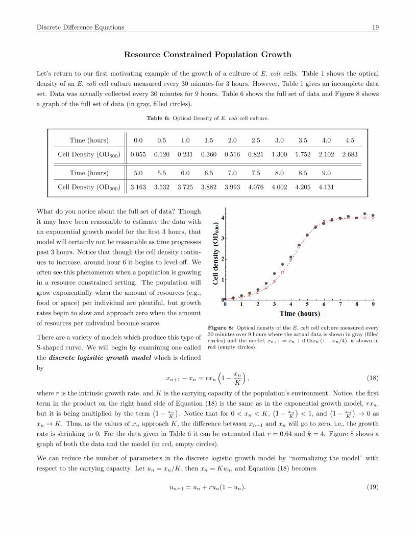
Resource Constrained Population Growth
Let’s return to our first motivating example of the growth of a culture of E. coli cells. Table 1 shows the optical
density of an E. coli cell culture measured every 30 minutes for 3 hours. However, Table 1 gives an incomplete data
set. Data was actually collected every 30 minutes for 9 hours. Table 6 shows the full set of data and Figure 8 shows
a graph of the full set of data (in gray, filled circles).
Table 6: Optical Density of E. coli cell culture.
Time (hours) 0.0 0.5 1.0 1.5 2.0 2.5 3.0 3.5 4.0 4.5
Cell Density (OD600) 0.055 0.120 0.231 0.360 0.516 0.821 1.300 1.752 2.102 2.683
Time (hours) 5.0 5.5 6.0 6.5 7.0 7.5 8.0 8.5 9.0
Cell Density (OD600) 3.163 3.532 3.725 3.882 3.993 4.076 4.002 4.205 4.131
Figure 8: Optical density of the E. coli cell culture measured every30 minutes over 9 hours where the actual data is shown in gray (filledcircles) and the model, xn+1 = xn + 0.65xn (1− xn/4), is shown inred (empty circles).
What do you notice about the full set of data? Though
it may have been reasonable to estimate the data with
an exponential growth model for the first 3 hours, that
model will certainly not be reasonable as time progresses
past 3 hours. Notice that though the cell density contin-
ues to increase, around hour 6 it begins to level off. We
often see this phenomenon when a population is growing
in a resource constrained setting. The population will
grow exponentially when the amount of resources (e.g.,
food or space) per individual are plentiful, but growth
rates begin to slow and approach zero when the amount
of resources per individual become scarce.
There are a variety of models which produce this type of
S-shaped curve. We will begin by examining one called
the discrete logisitic growth model which is defined
by
xn+1 − xn = rxn
(1− xn
K
), (18)
where r is the intrinsic growth rate, and K is the carrying capacity of the population’s environment. Notice, the first
term in the product on the right hand side of Equation (18) is the same as in the exponential growth model, rxn,
but it is being multiplied by the term(1− xn
K
). Notice that for 0 < xn < K,
(1− xn
K
)< 1, and
(1− xn
K
)→ 0 as
xn → K. Thus, as the values of xn approach K, the difference between xn+1 and xn will go to zero, i.e., the growth
rate is shrinking to 0. For the data given in Table 6 it can be estimated that r = 0.64 and k = 4. Figure 8 shows a
graph of both the data and the model (in red, empty circles).
We can reduce the number of parameters in the discrete logistic growth model by “normalizing the model” with
respect to the carrying capacity. Let un = xn/K, then xn = Kun, and Equation (18) becomes
un+1 = un + run(1− un). (19)

Discrete Difference Equations 20
Not we refer to replacing xn with Kun as either a substitution or change of variables. What is the equilibrium of
the normalized discrete logistic model? Recall, the equilibrium occurs when un+1 = un. Let u∗ be such a value.
Then,
u∗ = u∗ + ru∗(1− u∗) ⇒ 0 = ru∗(1− u∗),
which will hold true when u∗ = 0 or u∗ = 1. Thus, the normalized discrete logistic model has two equilibria: (1)
when the population size is 0 (i.e., extinct), and (2) when the population size has reached carrying capacity.
Example 7.Use cobweb diagrams and sequence plots to explore the dynamics of the normalized discrete logistic model as the parameter value r is
increased from 0.2 to 3.1.
The solutions to this example will be worked in class.
Exercise 9 – Beverton-Holt Difference Equation
Figure 9: Plot of sequence produced bythe Beverton-Holt difference equation.
The Beverton-Holt difference equation is another commonly used for modeling the growth of a
population in a resource constrained setting. The Beverton-Holt difference equation is
xt+1 =rxt
1 + r−1Kxt, (20)
where r is the intrinsic growth rate, and K is the carrying capacity.
(a) Show that the substitution ut = 1/xt transforms Equation (20) into a linear difference
equation (i.e., it has the form ut+1 = aut + b, where a and b are in terms of r and K).
(b) Given the linear difference equation you generated in part (a), find the closed form solution
to the Beverton-Holt equation.
(c) Find the equilibrium for the transformed Beverton-Holt equation. Interpret this equilib-
rium in terms of the original Beverton-Holt equation.
(d) The original Beverton-Holt has an additional equilibrium. What is it?
(e) To determine the stability of each equilibria, consider two cases: (i) r > 1, and (2) r < 1.
Use the closed form solution of the Beverton-Holt equation to determine the stability of
each equilibria in each case.
(f) Use Matlab to plot the sequences generated by the Beverton-Holt difference equation and
the logistic difference equation for x0 = 0.2, K = 1, and (i) r = 0.25, (ii) r = 0.75, (iii)
r = 1.25, (iv) r = 1.90, (v) r = 2.20, (vi) r = 2.50, and (vii) r = 3.00. Describe the ways
in which the Beverton-Holt and logistic difference equations are similar and the ways in
which they are different.
Natural Selection
Recall in Section 7 we examined the Hardy-Weinberg model. The model had eight assumptions, and when we
relaxed the “no migration” assumption (Assumption #6) we developed the continent-island model. In this section,
we will develop a model for when we relax the “no natural selection” assumption (Assumption #8). Recall that
natural selection refers to a consistent (i.e., over multiple generations) relationship between fitness and phenotype,
or differences in fitness among genotypes.
Let A and a be the two possible alleles for a particular gene of interest where A is the dominant allele and a is the
recessive allele. Let pt be the allele frequency of A in generation t, and qt = 1 − pt be the allele frequency of a in

Discrete Difference Equations 21
Table 7: Genotype frequencies in generation t+ 1 with and without natural selection, where w̄ = w1p2t + 2w2ptqt + w3q2t .
AA Aa aa
Frequency in absence of natural selection p2t 2ptqt q2t
Relative fitness of genotype w1 w2 w3
Frequency with natural selection w1p2tw̄
2w2ptqt
w̄
w3q2tw̄
generation t. In the absences of natural selection, according to the Hardy-Weinberg model, the frequency of each
possible genotype (AA, Aa, and aa) in generation t+ 1 are given in Equations (14) - (16), and shown again in Table
7. In the presence of natural selection, each genotype may confer a different relative fitness (relative with respect
to the other genotypes). Let w1 be the relative fitness of genotype AA, w2 the relative fitness of genotype Aa, and
w3 the relative fitness of genotype w3. We define the mean fitness of the population, w̄, as the sum of the relative
contributions of each genotype, that is,
w̄ = w1p2t + 2w2ptqt + w3q
2t . (21)
Then, the frequency of each genotype in the presence of natural selection is the ratio of the relative contribution of
each genotype to the mean fitness (see Table 7). Thus, in the presence of natural selection we have that
Pt+1 =w1p
2t
w̄, Qt+1 =
2w2ptqtw̄
, and Rt+1 =w3q
2t
w̄. (22)
Notice that, as with the Hardy-Weinberg model (without selection), Pt+1 +Qt+1 +Rt+1 = 1.
As with the continent-island model, let us form construct a difference equation to model the frequency of the
recessive allele, a, over several generations. This time we will assume there is no gene flow, but that there is natural
selection.
qt+1 =1
2Qt+1 +Rt+1 =
w2ptqt + w3q2t
w1p2t + 2w2ptqt + w3q2t(23)
Equation (23) expresses qt+1 as a function of pt and qt. To express qt+1 solely as a function of qt we can use the fact
that pt = 1− qt, and thus,
qt+1 =w2 (1− qt) qt + w3q
2t
w1 (1− qt)2 + 2w2 (1− qt) qt + w3q2t. (24)
We will refer to Equation (24) as the natural selection difference equation model .
Table 8: Relative fitness values for different fitness relationships.
Genotype
AA Aa aa
General relative fitness w1 w2 w3
Lethal recessive 1 1 0
Detrimental alleles (recessive) 1 1 1− s
Detrimental alleles (additive) 1 1− s/2 1− s
Dominance (purifying selection) 1 1− hs 1− s
Dominance (positive selection) 1 + s 1 + hs 1
Heterozygote advantage 1− s1 1 1− s2
Heterozygote disadvantage 1 + s1 1 1 + s2
We can change of the relative fitness values of w1, w2,
and w3 (mathematically described as weight values or
weight constants) to reflect different “fitness relation-
ships” between genotypes. Recall that the values of w1,
w2, and w3 reflect the relative fitness of each genotypes.
Thus, if two genotypes have the same relative fitness,
their weight values should be the same. If one genotype
has a greater fitness than another, than the relative fit-
ness of the former genotype should be larger than that
of the latter genotype. The relative fitnesses of each

Discrete Difference Equations 22
genotype for several different types of fitness relation-
ships are shown in Table 8. The parameter s, called the
selection coefficient , is a measure of the amount of
selection against the recessive allele a (or for the domi-
nant allele A). The parameter h is called the level of dominance , and when multiplied by s measures the amount of
selection against the heterozygote. We will explore some of the fitness relationships in Table 8 through the following
examples and exercises.
Example 8.
Figure 10: The frequency of the recessive (lethal)glued allele for two D. melanogaster population repli-cates each starting with all heterozygotes (q0 = 0.5).
Lethal Recessive Submodel · There are some genes for which the homozy-
gous recessive genotype has the phenotype of a lethal disease which causes pre-
reproductive death, resulting in the fitness of the homozygous recessive genotype
being 0, i.e., w3 = 0. Some examples of such diseases in humans are Tays-Sachs
disease and cystic fibrosis.
In Drosophila melanogaster (also known as the common fruit fly or vinegar fly),
the homozygous recessive genotype of the gene glued causes pre-reproductive
death, and the heterozygous genotype reduces eye size and affects eye appear-
ance. Two replicate populations of Drosophila melanogaster were initiated with
all heterozygotes so that q0 = 0.5. The frequency of the recessive allele was
recorded for 7 successive generations for each replicate population (data shown
in Figure 10). We will compare two different lethal recessive submodels of the
natural selection difference equation model and determine which more accu-
rately represents the data shown.
(a) For the first model, we will assume that the recessive allele only causes a reduction in fitness in the homozygous recessive genotype,
that is, the homozygous dominant and heterozygous genotypes have the same relative fitness: w1 = 1, w2 = 1, and w3 = 0. Given
the values of w1, w2, and w3, simplify Equation (24), and determine a closed form solution. What happens to the values of qt as
t→∞?
(b) For the second model, we will assume that in additional to the lethality of the homozygous recessive genotype the defects in the
heterozygotes (reduced eye size and altered eye appearance) cause a reduction in fitness in the heterozygotes such that w1 = 1,
w2 = 2/3, and w3 = 0. Note, this would be a case of “dominance (purifying selection)” with s = 1 (lethal recessive) and h = 2/3.
Given the values of w1, w2, and w3, use a cobweb diagram to determine what happens to the values of qt as t→∞.
(c) Which model best describes the data shown in Figure 10?
(d) For each model calculate the number of generations needed for the recessive allele frequency to fall below 0.01. Which fitness
relationship removes the recessive allele frequency from the population more quickly? Does this make intuitive sense?
The solutions to this example will be worked in class.
Example 9.Detrimental Recessive Submodel · In many instances, there is no complete selection against the homozygous recessive genotype,
and thus, the relative fitness of the homozygote is only partially reduced (when compared with other genotypes). For many human
genetic diseases, such as albinism and sickle cell anemia, homozygous recessive individuals can survive and produce progeny, although
the probability of this occurring is reduced compared with that of other individuals. In Drosophila, mice, corn, and other organisms that
have been investigated in detail genetically, there are many examples of recessive morphologic mutants that reduce fitness of homozygotes
but do not cause lethality. In the case of a detrimental (but non-lethal) recessive allele, w1 = 1, w2 = 1, w3 = 1− s, where 0 < s < 1.
(a) Given the values of w1, w2, and w3, simplify Equation (24) to form the detrimental recessive submodel.
(b) What are the equilibria of the detrimental recessive submodel?
(c) Use a cobweb diagram to determine what happens to the values of qt as t → ∞ for different values of q0 and s. What affect does
increasing the value of s have on the model?

Discrete Difference Equations 23
The solutions to this example will be worked in class.
Exercise 10 – Heterozygous Advantage
Figure 11: Polymorphs of the common buzzard.
A rare example of heterozygote advantage in a natural population is the plumage
polymorphism in common buzzards (Buteo buteo) in Europe. Buzzard feathers
vary from dark brown to almost pure white, and much of this variation is due to
a single gene with two alleles: D (dark feathers, dominant) and d (light feathers,
recessive). The relative fitness for the different genotypes are w1 = 0.45 (DD),
w2 = 1 (Dd), and w3 = 0.54 (dd).
(a) Given the values of w1, w2, and w3, simplify (24).
(b) What are the equilibria of the model in part (a)?
(c) Use a cobweb diagram to determine what happens to the value of qt as
t→∞ for different values of q0. Which equilibria are stable and which are
unstable?
(d) Suppose the allele frequency reaches equilibrium within the population,
which equilibrium would you expect to see in the population? If the allele
frequency in the population is at equilibrium, then the genotype frequen-
cies are also in equilibrium. Use Equations 22 to determine the genotype
frequencies at equilibrium.
Exercise 11 – Blood Type Rh Factor
In mammals, there are interactions between a mother and her fetus that influence the survival of offspring of particular genotypes. The
best understood maternal-fetal incompatibility system is the Rh (rhesus) blood group system on the short arm of chromosome 1 in
humans. The the RHD gene of the Rh system gives the + or – in the human blood type. The dominant allele R indicates the presence
of antigen D from gene RHD, while the recessive allele r indicates the absence of antigen D. Fetal mortality occurs when the fetus is
Rh positive (genotype RR or Rr) and the mother is Rh negative (genotype rr) and the maternal antibody production of D destroys
the red blood cells of the fetus. Incompatible combinations only occur when the mother is Rh negative and the father is Rh positive.
Approximately 10% to 15% of the matings in most Caucasian populations are incompatible.
Incompatible combinations can only occur when the mother is Rh negative and the father is Rh positive, that is matings RR(♂)× rr(♀)
and Rr(♂)× rr(♀). In the matings RR(♂)× rr(♀), all offspring are incompatible with the mother (since all progeny have genotype Rr
which is Rh positive). In the matings Rr(♂)×rr(♀), half of all offspring are Rr while the other half are rr. Thus, only half of the progeny
are Rh positive and incompatible with the mother. Since a mother who is Rh negative will never produce progeny with genotype RR,
selection is only occurring against heterozygous progeny.
(a) Assuming relative fitnesses of w1 = 1 + s1, w2 = 1, and w3 = 1 + s2, simplify Equation (24) to form the heterozygous disadvantage
model.
(b) Find all equilibria for the model you formed in (a). Hint: There are 3 equilibria, and you will need to use the quadratic formula to
find two of them.
(c) Assume that s1 = 1 and s2 = 0.5 use a cobweb diagram to determine the stability of each of the equilibria.
(d) Most human populations have high frequencies of the R allele, but Basques, who live in the Pyrenees Mountains between Spain
and France, have a high frequency (q = 0.65) of the r allele. Assuming that the allele frequency of r in Pyrenees Moutain Basque
population is at equilibrium determine an expression for the relationship between s1 and s2 using the non-trivial equilibrium found
in part (b). Is the advantage greater for the homozygous dominant or homozygous recessive genotype?

Discrete Difference Equations 24
9 Systems of Difference Equations
Biological processes rarely happen in isolation. Interactions such as those between predators and prey, competitors
for limited resources, and many biochemical processes at the cellular level are major drivers of biological complexity.
These interactions are also rarely linear; that is, we typically cannot derive how one process affects another by
assuming that one is proportional to the other. In this section we will explore how we can use discrete difference
equations to model a biological system consisting of multiple species, classes, or organism groups.
Predator-Prey Systems
(a) Pelt-trading records of the Hudson Bay Com-pany for Canadian lynx (red) and snowshoe hares(blue).
(b) Lynx catching a hare for his mid-afternoonsnack.
A classic example of predator-prey system dynamics can be found
in the Canadian lynx (Lynx canadensis) and snowshoe hare (Lepus
americanus) pelt-trading records of the Hudson Bay Company (see
Figure 12a, thousands of lynx pelts shown in red and thousands of
hare pelts shown in blue). The primary food source for the Canadian
lynx is the snowshoe hare. If we think of the number of pelts of each
species harvested each year by the Hudson Bay Company as being
representative of the respective population sizes (obviously the total
popualtion sizes are larger than the number of pelts caught), then
we can use the pelt data to inform a model of the population sizes
of both the lynx and the hares.
Examine the data in Figure 12a. What do you notice? You should
observe that both populations cycle over roughly a 10 year period.
Additionally, the cycles in the lynx pelts harvested (on average) lags
behind the cycles in the hare pelts harvested by 1 to 3 years.
In 1920 Alfred J. Lotka (a mathematician and physical chemist) pro-
posed a set of ordinary differential equations to model the dynamics
of an herbivorous animal species and the plant species it consumed.
In 1926, Vito Volterra (a mathematician and physicist) indepen-
dently investigate similar equations as applied to fish catches in the
Adriatic. If you have taken a Calculus II course or a Differential Equations course, you have likely seen the classic
Lotka-Volterra equations. In this course, we will examine the discrete difference equation analog of the Lotka-Volterra
model,
xn+1 = rxn − αxnyn (prey population size or density) (25)
yn+1 = syn + βxnyn (predator population size or density) (26)
where r > 1 is the growth rate of the prey in the absence of the predator, 0 < s < 1 is the survival rate of the
predator in the absence of its prey source, α > 0 is the consumption rate of the predators (where αxn is the average
number of prey eaten per predator in time step n), and β > 0 is the growth rate of the predator population due to
the consumption of prey. Notice the amount of prey consumed by the predator at each time step depends on not
only on the numbers of predators present, but also the numbers of prey present. When the prey density is higher, it

Discrete Difference Equations 25
is easier for the predators to find prey and thus more prey will be consumed. Likewise, the growth rate the predators
depends not only on the number of predators present (more predators should produce more offspring overall), but
also on the number of prey present (a large food source often correlates with higher reproductive rates and/or larger
litter or clutch sizes).
Figure 13: Plot of the sequences produced by thediscrete Lotka-Volterra model, Equations (25) - (26),with r = 1.0015, s = 0.9994, α = 0.0006, β = 0.00025,and each time step represents 14.6 hours (a little morethan half a day).
We will use this model, Equations (25) - (26), to demonstrate how
to find the equilibria of a system of difference equations. However,
the discrete Lotka-Volterra (like the discrete logistic) becomes unre-
alistic (negative population sizes, or unrealistically large population
sizes) with many parameters sets (i.e., the values of r, s, α, and β).
A simulation for one parameter set is shown in Figure 13, but in
order for the model to remain realistic, the time step must be scaled
to represent 14.6 hours (a little more than half a day). Notice also
that population density (not population size) is shown. The initial
conditions, x0 = 2 and y0 = 3, implies that the initial ratio of prey
individuals to predator individuals (per unit area) is 2:3.
To find the equilibria of the discrete Lotka-Volterra model, recall
that an equation is at an equilibrium when the variable remains
constant from one time step to the next. Thus, (x∗, y∗) is an equilibrium to the system xt+1 = f(xt, yt) and
yt+1 = g(xt, yt), where f and g are functions, if f(x∗, y∗) = x∗ and g(x∗, y∗) = y∗. For Equations (25) - (26) this
means
x∗ = rx∗ − αx∗y∗
x∗ − rx∗ + αx∗y∗ = 0
x∗ (1− r + αy∗) = 0
Thus, either x∗ = 0, or 1 − r + αy∗ = 0. The second
equation implies y∗ = (r − 1)/α.
y∗ = sy∗ + βx∗y∗
y∗ − sy∗ − βx∗y∗ = 0
y∗ (1− s− βx∗) = 0
Thus, either y∗ = 0, or 1 − s − βx∗ = 0. The second
equation implies x∗ = (1− s)/β.
Any equilibrium point of the system must satisfy both equation (x∗ = rx∗ − αx∗y∗ and y∗ = sy∗ + βx∗y∗) simulta-
neously. The algebra above shows us we should consider four different cases: (1) x∗ = 0 and y∗ = 0, (2) x∗ = 0 and
y∗ 6= 0 (i.e. 1− s− βx∗ = 0), (3) x∗ 6= 0 (i.e. 1− r + αy∗ = 0) and y∗ = 0, and (4) x∗ 6= 0 and y∗ 6= 0.
Case 1: If x∗ = 0 and y∗ = 0, then both equations are satisfied simultaneously, and (0, 0) is an equilibrium.
Case 2: Suppose x∗ = 0 and y∗ 6= 0. If y∗ 6= 0, then x∗ = (1− s)/β which cannot be true since x∗ = 0. Thus, we
cannot have an equilibrium where x∗ = 0 and y∗ 6= 0.
Case 3: Suppose x∗ 6= 0 and y∗ = 0. If x∗ 6= 0, then y∗ = (r − 1)/α which cannot be true since y∗ = 0. Thus, we
cannot have an equilibrium where x∗ 6= 0 and y∗ = 0.
Case 4: If x∗ 6= 0 and y∗ 6= 0, then x∗ = (1 − s)/β and y∗ = (r − 1)/α, and both equations are satisfied
simultaneously. Thus, ((1− s)/β, (r − 1)/α) is an equilibrium.

Discrete Difference Equations 26
Therefore, the two equilibria of the discrete Lotka-Volterra model are (0, 0), which we will refer to at the trivial
equilibrium , and ((1− s)/β, (r − 1)/α).
Example 10.Consider a discrete-time predator-prey model in which the prey grows logistically in the absence of the predator, that is
xt+1 = rxt(1− xt)− αxtyt
yt+1 = syt + βxtyt,
where r > 1, 0 < s < 1, α > 0, and β > 0 are defined the same as in the discrete Lotka-Volterra.
(a) Find all equilibria of this predator-prey model.
(b) Let x0 = 0.6 and y = 0.1 (where x and y represent population densities). To answer each of the following make a time series plot
of each population over at least 50 time steps. Additionally, make a plot of yt vs. xt over the same number of time steps. Plot the
equilibria points on the second plot.
(i) Describe the dynamics of each population when r = 2, s = 0.8, α = 0.5, β = 1.5. What is the long-term behavior of the model?
(ii) Describe the dynamics of each population when r = 2, s = 0.8, α = 0.5, β = 2.5. What is the long-term behavior of the model?
(iii) Describe the dynamics of each population when r = 2, s = 0.8, α = 1.8, β = 2.5. What is the long-term behavior of the model?
The solutions to this example will be worked in class.
Exercise 12 – A Competition Model
One way that multiple populations interact is through predator-prey interactions as we explored above. However, another way that
multiple populations can interact is through competition for resources. For example, if two populations both feed upon a the same
resource, or if two populations establish nests, burrows, dens, etc. in the same spatial range. Consider the Leslie-Gower difference
equation competition model,
xt+1 =b1xt
1 + xt + c1ytand yt+1 =
b2yt
1 + c2xt + yt,
where xt and yt are the densities of two competing populations, and all the parameters (b1, b2, c1, and c2) are positive.
(a) Assume there is only one population, i.e. yt = 0 for all t. Simplify the equation for the x population. What is the equilibrium of
this population? Use cobweb diagramming to determine the stability of each equilibria (Hint: Each equilibria will be stable under
certain conditions). Based on your examination of the model so far what does the remaining parameter in the equation represent?
(b) What happens to the x population if the parameter value c1 is increased? What happens to the y population if the parameter value
c2 is increased? If b1 = b2 and c1 > c2 what do you think will happen to the two competing species?
(c) Find all equilibria of the competition model.
(d) Create a plot of yt vs. xt and additionally plot each of the equilibria points on this graph. For each of the following parameter sets,
indicate which equilibria are in the first quadrant (i.e., biologically reasonable), and which equilibria is approached as t → ∞. You
should examine several different initial conditions for each parameter set (always choose x0 > 0 and y0 > 0).
(i) b1 = b2 = 2, c1 = 0.4, and c2 = 0.6
(ii) b1 = b2 = 2, c1 = 1.4, and c2 = 0.6
(iii) b1 = b2 = 2, c1 = 0.4, and c2 = 1.6
(iv) b1 = b2 = 2, c1 = 1.4, and c2 = 1.6

Discrete Difference Equations 27
Allele Frequencies of Sex-Linked Genes
Figure 14: Sex chromosomes in different species.
In dioecious organisms (those species with two sexes for which one
member of each sex is required for reproduction), sex is determined
by a difference in the chromosomes of each sex. The form that
these difference take vary among different species. In many animals
(humans included), sex is determined by a single chromosome which
we will refer to as the sex-chromosome, the remaining chromosomes
are referred to as autosomes.
In grasshoppers the females have two X chromosomes, while the
males only have one. The eggs formed by the females have one copy
of each autosome, plus one X chromosome. The males form two
types of sperm (in roughly equal amounts): one which contains one
copy of each autosome plus one X chromosome, and the other which only contains one copy of each autosome. When
a sperm containing an X chromosome fertilizes an egg, the egg develops into a female grasshopper. When a sperm
which does not contain an X chromosome fertilizes an egg, a male grasshopper develops. We will refer to the female
grasshoppers as being XX, and the male grasshoppers as being XO.
In mammals (including humans), females have two X chromosomes and males have one X chromosome and one Y
chromosome. Both males and females have two copies of each autosome. Like the grasshoppers, mammal males
produce two types of sperm, but in this case one which contains one copy of each autosome plus one X chromosome,
and the other which contains one copy of each autosome plus one Y chromosome. Here, we refer to female mammals
as being XX, and male mammals as being XY.
In birds, butterflies, and moths, the females are XY and the males are XX. To avoid confusion, we use a different
set of letters for these species. We will refer to females as ZW, and males as ZZ.
For the following discussion we will assume that females are XX and males are XO or XY. When the locus of a gene
occurs on one of the sex chromosomes, we must modify the Hardy-Weinberg model. Recall that Assumption #4 of
the Hardy-Weinberg model was, “Allele frequencies are the same in both sexes.” If the locus of a gene occurs on
the X chromosome, then the females will have two alleles for that gene and the males will only have one allele for
that gene. This will necessarily alter the allele frequencies between the sexes and we must account for this in the
model.
Let P ft , Hft , and Qft represent the diploid genotype frequencies AA, Aa, and aa in the females of the population in
generation t, and Pmt and Qmt represent the haploid genotype frequencies A and a in the males of the population in
generation t. Then, the allele frequencies in each of the sexes in generation t are
(♀, A) pft = P ft +1
2Hft and (♂, A) pmt = Pmt ,
(♀, a) qft = Qft +1
2Hft and (♂, a) qmt = Qmt .
If we assume that there are an equal number of males and females in each generation, then two-thirds of the alleles
are in the females and one-third of the alleles are in the males, and thus the frequencies of alleles A and a in the
population in generation t are
pt =2
3pft +
1
3pmt and qt =
2
3qft +
1
3qmt ,

Discrete Difference Equations 28
respectively. To determine the allele frequencies in the next generation (t+ 1), we start by examining the genotype
frequencies in generation t+ 1. Table 9 shows the genotype frequencies in males and females of generation t+ 1 sort
by mating type. For example, given a AA(♀) × a(♂) mating (row 2 in Table 9), the only possible genotype of the
offspring is Aa in the females and A in the males (remember, the males get their X chromosome from their mother
and their Y chromosome from their father). Since the genotype frequency of AA in females in generation t is P ft ,
and the genotype frequency of a in males in generation t is Qmt , the probability of a AA(♀)× a(♂) mating is P ft Qmt .
The frequency of female (and male) offspring from this type of mating is the probability of this mating type, i.e.
P ft Qmt . Since there is only one female genotype resulting from this type of mating (Aa), the frequency of the Aa
genotype in female offspring resulting from a AA(♀)× a(♂) mating is P ft Qmt . Likewise, since there is only one male
genotype resulting from this type of mating (A), the frequency of the A genotype in male offspring resulting from a
AA(♀)× a(♂) mating is also P ft Qmt .
In contrast to this, consider a Aa(♀) × A(♂) mating (row 3 in Table 9). Since the genotype frequency of Aa in
females in generation t is Hft , and the genotype frequency of A in males in generation t is Pmt , the probability of a
Aa(♀)×A(♂) mating is Hft P
mt . From this type of mating (on average) half of the female offspring will have genotype
AA and half will have genotype Aa. Thus, the frequencies of the AA and Aa genotypes in female offspring are both12H
ft P
mt . Likewise, from this type of mating (on average) half of the male offspring will have genotype A and half
will have genotype a. Thus, the frequencies of each genotype in male offspring is 12H
ft P
mt .
Table 9: Genotype frequencies of offspring for a gene on an X chromosome assuming random mating with ♀ XX and ♂ XY or XO.
Mating Type Female Offspring Male Offspring
♀ ♂ Frequency AA Aa aa A a
AA×A P ft P
mt P f
t Pmt — — P f
t Pmt —
AA× a P ft Q
mt — P f
t Qmt — P f
t Qmt —
Aa×A Hft P
mt
12Hf
t Pmt
12Hf
t Pmt — 1
2Hf
t Pmt
12Hf
t Pmt
Aa× a Hft Q
mt — 1
2Hf
t Qmt
12Hf
t Qmt
12Hf
t Qmt
12Hf
t Qmt
aa×A Qft P
mt — Qf
t Pmt — — Qf
t Pmt
aa× a Qft Q
mt — — Qf
t Qmt — Qf
t Qmt
Total 1 pft pmt pft q
mt + qft p
mt qft q
mt pft qft
In the final row of Table 9 we calculate the frequency of each genotype in each of the sexes. For example, the
genotype frequency of AA in female offspring (generation t+1) is found by summing all the frequencies in the AA(♀)
column.
P ft+1 = P ft Pmt +
1
2Hft P
mt =
(P ft +
1
2Hft
)Pmt = pft p
mt .
Similarly, the genotype frequency of A in male offspring is
Pmt+1 = P ft Pmt + P ft Q
mt +
1
2Hft P
mt +
1
2Hft Q
mt =
(P ft +
1
2Hft
)(Pmt +Qmt ) = pft ,
since Pmt +Qmt = 1. Using the fact that pft + qft = 1 and pmt + qmt = 1, we can now calculate the allele frequencies

Discrete Difference Equations 29
of a in both the females and males in generation t+ 1,
qft+1 = Qft+1 +1
2Hft+1 = qft q
mt +
1
2
(1− qft
)qmt +
1
2qft (1− qmt ) =
1
2
(qft + qmt
),
qmt+1 = Qmt = qft .
As with the predator-prey system we now have a system of difference equations. The value of qf in the next generation
depends on the values of qf and qm in the current generation, and the value of qm in the next generation depends
on the value of qf in the current generation.
Example 11.Show that the system of difference equations
qft+1 =1
2
(qft + qmt
)and qmt+1 = qft
has infinitely many points of equilibrium. Then, test many different initial conditions, (qf0 , qm0 ), and devise a rule of thumb for the value
of the equilibrium point given the initial conditions. The solutions to this example will be worked in class.
Example 12.An interesting example of a gene residing on the X chromosome is the orange coat-color locus in cats. This gene has two alleles, O
which codes for an orange coat, and b which codes for a black coat. Females with the heterozygous genotype Ob have tortoise-shell or
calico coats. In a population of feral London cats, the sex and genotype of cats sent to a clinic for “destruction” were noted by a clinic
worker. PSA: If hearing about cats being sent to clinics for destruction (and yes, that means what you think it means) makes you sad,
you should advocate for spaying and neutering cats. Most medium to large cities in the United States have free/low cost spaying and
neutering programs to help reduce feral cat population sizes.
Genotype OO(♀) OB(♀) BB(♀) O(♂) B(♂)
# Observed 7 54 277 42 311
(a) Determine the genotype frequencies of each genotype for both male and females.
(b) Let qft represent the frequency of the O allele in the females in generation t, and qmt the frequency of the allele O in the males in
generation t. If the data presented above were collected over a short period of time, we can assume it represents one generation (we
will call it generation 0). Calculate the values of qf0 and qm0 .
(c) Given the values of qf0 and qm0 , and the system of difference equations
qft+1 =1
2
(qft + qmt
)and qmt+1 = qft
estimate the equilibrium point.
(d) At the equilibrium point, what proportion of females have tortoise-shell coats.
The solutions to this example will be worked in class.
Exercise 13 – Natural Selection on X-Linked Gene
The model for the allele frequencies of a gene on an X chromosome (an X-linked gene) assumes that the relative fitness of each of the
genotypes (for both males and females) are equal. However, this assumption is not always true. To model natural selection for an X-linked
gene we use a variation of the natural selection model in Equation (24),
qft+1 =
12w12
((1− qft )qmt + qft (1− qmt )
)+ w22q
ft q
mt
w11(1− qft )(1− qmt ) + w12
((1− qft )qmt + qft (1− qmt )
)+ w22q
ft q
mt
and qmt+1 =w2q
ft
w1(1− qft ) + w2qft
,

Discrete Difference Equations 30
where w11, w12, w22, w1, and w2 are the relative fitnesses of genotypes AA(♀), Aa(♀), aa(♀), A(♂), and A(♂), respectively. Let us
consider a case where selection occurs against the homozygous recessive genotype in females and against the recessive genotype in males,
i.e.,
w11 = 1, w12 = 1, w22 = 1− sf , w1 = 1, and w2 = 1− sm.
Figure 15: Drosophila melanogasterwith red eyes (left) and white eye (right).
(a) Given these relative fitnesses, simplify the natural selection model for an X-linked gene.
(b) Now, suppose the recessive allele is lethal, in that individuals with genotypes aa and a
do not survive to reproduce. Then sf = sm = 1. Further simplify the model assuming a
lethal recessive allele.
(c) Find thr equilibria of the system assuming a lethal recessive allele.
(d) An example of X-linked selection occurs in Drosophila melanogaster (commonly known
as fruit flies) on the white gene. The white gene controls eye color. The dominant allele A
codes for red eyes, but the recessive allele a codes for white eyes. The diploid genotypes
AA and Aa yield red-eyed females, while the aa genotype yields white-eyed females. The
haploid genotype A yields red-eyed males, while the genotype a yields white-eyed males. The selection acts primarily against the
white-eyed males by reducing their mating ability (sm = 0.9), however there is also some reduction in the fertility of white-eyed
females (sf = 0.5). Use Matlab to generate a plot of qft , qmt , and qt for t = 0, 1, . . . , 7 given (i) qf0 = qm0 = 0.833, and (ii) qf0 = 1,
qm0 = 0.5.

Discrete Difference Equations 31
References
[1] E.N. Bodine, S. Lenhart, and L.J. Gross. Mathematics for the Life Sciences. Princeton University Press, 2014.
[2] J.K. Conner and D.L. Hartl. A Primer of Ecological Genetics. Sinauer Associates, Inc., 2004.
[3] J.M. Cushing, S. Levarge, N. Chitnis, and S.M. Henson. Some discrete competition models and the competitive
exclusion principle. Journal of Difference Equations and Applications, 10(13–15): 1139–1151, 2004.
[4] F.R. Giordano, W.P. Fox, S.B. Horton, and M.D. Weir. A First Course in Mathematical Modeling, 4th Edition.
Brooks/Cole, 2009.
[5] P.W. Hedrick. Simulatoin of X-linked selection in Drosophila. Genetics, 83: 551-571, 1976.
[6] P.W. Hedrick. Genetics of Populations, 4th Edition. Jones & Bartlett, 2011.
[7] M. Kot. Elements of Mathematical Ecology. Cambridge University Press, 2001.
[8] http://www.fwrc.msstate.edu/predator/bobSurvive.asp

Discrete Difference Equations 32
Answer Key to Exercises
Exercise 1 – Wild Hares
(a) xn+1 = 1.12xn, x0 = 200
(b) xn = (1.12)n(200)
(c) x6 ≈ 395 hares
(d) xn →∞ as n→∞ which is not biologically reasonable. it is reasonable to assume that though growth may be
exponential for a time, at some point the hare population will begin to exceed the capacity of its environment
in terms of space or other resources (e.g., food), and thus limit reproduction or increase the death rate within
the population.
Exercise 2 – Elk Herd
(a) xn = (1.1)n(50); increasing sequence; x20 ≈ 336 elk
(b) xn = (0.9)n(50); decreasing sequence; x20 ≈ 6 elk; If the average lifespan of a wild elk is 15 years, there certainly
must be elk that live longer than 15 years. However, to truly test if the assumption in this case makes sense, we
would need to know the ages of the 50 elk that were originally introduced into the wildlife management area,
and an upper bound on the age of an elk in the wild. If most of the elk were already between over the age of 5,
then this model would predict that 6 of the original elk lived to be at least 25 years old. This is 10 years older
than the average and may or may not be reasonable.
Exercise 3 – Treating Heart Disease
(a) a = 0.69
(b) xn = 0.69n(0.5)
(c) Between 5 and 10 days
Exercise 4 – Buffalo
(a) xn = 800(1.1)n + 200
(b) No
(c) 100 buffalo
Exercise 5 – Trout
(a) n = 5
(b) 222 trout

Discrete Difference Equations 33
Exercise 6 – Cipro
(a) k ≈ 1.1, τ = 1, b = 500
(b) ≈ 746.3 mg
(c) Yes, the dosing scheme will need to be change. It can be changed by either lowering the dose size or increasing
the time between doses. If lowing the dose size, b would need to be lowered to below 469 mg. A safe dose would
be 450 mg. If increasing the time between doses, τ would need to be increased above 1.14 days (≈ 1 day, 3
hours, 22 minutes). This might be a difficult regime for the patient to follow. It may be reasonable to increase
the time between doses to 2 days, but it is unknown if this would allow the amount of Cipro in the bloodstream
to fall below its level of effectiveness.
Exercise 7 – Fire that Neuron
(a) xn+1 =(e−0.1
)xn + 1; xn =
1− e−0.1n
1− e0.1
(b) 10 milliseconds
Exercise 8 – Red Wolf Conservation
(a) m = 0.0375
(i) qt = (1−m)tq0 with q0 = 1; in 2040 (t = 10) 68% red wolf ancestry remains
(ii) qt = (1−m)tq0 with q0 = (1− 0.075)2; in 2040 (t = 8) 63% red wolf ancestry remains
(iii) qt = (1−m)tq0 with q0 = (1− 0.075)4; in 2040 (t = 6) 58% red wolf ancestry remains
(b) m = 0.0075
(i) qt = (1−m)tq0 with q0 = 1; in 2040 (t = 10) 93% red wolf ancestry remains
(ii) qt = (1−m)tq0 with q0 = (1− 0.075)2; in 2040 (t = 8) 81% red wolf ancestry remains
(iii) qt = (1−m)tq0 with q0 = (1− 0.075)4; in 2040 (t = 6) 70% red wolf ancestry remains
Exercise 9 – Beverton-Holt Difference Equation
(a) Let ut = 1/xt, then xt = 1/ut. Substitute xt = 1/ut into Equation (20) and simplify to obtain ut+1 = 1rut+
r−1K .
(b) ut =(u0 − 1
K
) (1r
)t+ 1
K ⇒ xt = K
1+(u0K−1)( 1r )
t
(c) u∗ = 1K (transformed Beverton-Holt), thus x∗ = K (original Beverton-Holt). This means that the equilibrium
of the Beverton-Holt model is the carrying capacity of the model.
(d) x0 = 0; This is often called the trivial equilibrium.
(e) (i) If r > 1, then 1r < 1 and
(1r
)t → 0 as t → ∞, and thus xt → K as t → ∞. (ii) If r < 1, then 1r > 1 and(
1r
)t →∞ as t→∞, and thus xt → 0 as t→∞.

Discrete Difference Equations 34
(f)
Exercise 10 – Heterozygous Advantage
(a) qt+1 =qt (1− 0.46qt)
0.45 + 1.1qt − 1.01q2t
(b) q∗ = 0, 55/101 (≈ 0.545), 1
(c) qt → 55/101 as t→∞, q∗ = 0 unstable, q∗ = 55/101 stable, q∗ = 1 unstable
(d) Expect to see q∗ = 55/101 in the population since it is the stable equilibrium. Genotype frequencies at equilibrium:
P ∗ = 0.12454 (DD), Q∗ = 0.66181 (Dd), R∗ = 0.21365 (dd)
Exercise 11 – Blood Type Rh Factor
(a) qt+1 =qt + s2q
2t
1 + s1 (1− qt)2 + s2q2t
(b) q∗ = 0,s1
s1 + s2, 1
(c) q∗ = 0 stable, q∗ = 2/3 unstable, q∗ = 1 stable
(d) s2 = 7s1/13, the advantage is greater for the homozygous dominant genotype
Exercise 12 – A Competition Model

Discrete Difference Equations 35
(a) xt+1 = b1xt
1+xt; the equilibria are x∗ = 0, b1 − 1;
x∗ = 0 is stable when 0 < b1 < 1, x∗ = b1 − 1 is stable when b1 > 1, and when b = 1 the only equilibrium is
x∗ = 0 which is stable in this case; The parameter b1 acts like a growth rate, and when b1 > 1 the populations
is growing and when 0 < b1 ≤ 1 the population is declining to extinction.
(b) As the value of c1 is increased the value of xt+1 decreases. The parameter c1 is a measure of the severity with
which x’s competition with y reduces the growth of x. Likewise, as the value of c2 is increased, the value of yt+1
decreases, and the parameter c2 is a measure of the severity with which y’s competition with x reduces the growth
of y. If the growth rates of the two populations are the same (b1 = b2), then the fate of the populations comes
down to who has a competitive advantage, which is population y when c1 > c2. We would expect population y
to grow more quickly than population x, and possibly even drive population x to extinction.
(c) (x∗, y∗) = (0, 0) , (0, b2−1), (b1−1, 0),
(b1 − b2c1 + c1 − 1
1− c1c2,b2 − b1c2 + c2 − 1
1− c1c2
); Notice that if b1 < 1, then the
equilibrium (b1−1, 0) is not biologically reasonable as it implies x∗ < 0. Likewise, if b2 < 1, then the equilibrium
(0, b2 − 1) is not biologically reasonable. Notice that under certain parameter sets, the fourth equilibrium does
not reside in the first quadrant and is thus biologically unreasonable. If you want an extra exercise, show that
when b1 = b2, the fourth equilibrium will be in the first quadrant when c1 < 1 < 1/c2.
(d) EQ1 = (0, 0), EQ2 = (0, b2 − 1), EQ3 = (b1 − 1, 0), and EQ4 =
(b1 − b2c1 + c1 − 1
1− c1c2,b2 − b1c2 + c2 − 1
1− c1c2
)(i) All four equilibria are in the first quadrant. All initial conditions lead to EQ4.
(ii) EQ4 is no longer in the first quadrant. All initial conditions lead to EQ2.
(iii) EQ4 is no longer in the first quadrant. All initial conditions lead to EQ3.
(iv) All four equilibria are in the first quadrant. The equilibria that is approaches as t → ∞ is determined by
the relative position of (x0, y0) with respect to the line y0 = b2−b1c2+c2−1b1−b2c1+c1−1x0 = 1.5x0. When y0 < 1.5x0,
then solutions approach EQ3; When y0 = 1.5x0, then solutions approach EQ4; When y0 > 1.5x0, then
solutions approach EQ2.
Exercise 13 – Natural Selection on X-Linked Gene
(a) qft+1 =12 (qft + qmt )− sfqft qmt
1− sfqft qmtand qmt+1 =
(1− sm)qft
1− smqft(b) qft+1 = 1
2qft and qmt = 0
(c) (0, 0) is the only equilibria
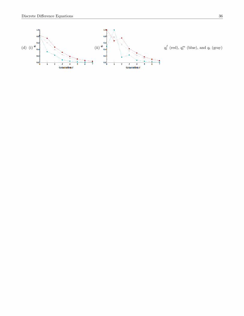
Discrete Difference Equations 36
(d) (i) (ii) qft (red), qmt (blue), and qt (gray)