Discovering Binary Codes for Documents by …rsalakhu/papers/topics.pdf · Discovering Binary Codes for Documents by Learning Deep Generative Models Geoffrey Hinton,a Ruslan Salakhutdinovb

Discovering Binary Codes for Documents by LearningDeep Generative Models

Geoffrey Hinton,a Ruslan Salakhutdinovb

aDepartment of Computer Science, University of TorontobDepartment of Brain and Cognitive Sciences, Massachusetts Institute of Technology

Received 12 March 2009; received in revised form 8 January 2010; accepted 8 January 2010

Abstract

We describe a deep generative model in which the lowest layer represents the word-count vector

of a document and the top layer represents a learned binary code for that document. The top two lay-

ers of the generative model form an undirected associative memory and the remaining layers form a

belief net with directed, top-down connections. We present efficient learning and inference proce-

dures for this type of generative model and show that it allows more accurate and much faster retrie-

val than latent semantic analysis. By using our method as a filter for a much slower method called

TF-IDF we achieve higher accuracy than TF-IDF alone and save several orders of magnitude in

retrieval time. By using short binary codes as addresses, we can perform retrieval on very large

document sets in a time that is independent of the size of the document set using only one word of

memory to describe each document.

Keywords: Deep learning; Semantic hashing; Auto-encoders; Restricted Boltzmann machines;

Document retrieval; Binary codes

1. Introduction

Representing the semantic content of a document is an unsolved problem. We think it is

very unlikely that a low-dimensional representation containing only a few hundred numbers

will ever be capable of capturing more than a tiny fraction of the content of the distributed

representation over millions of neurons that is used by the brain. Even if the documents do

lie on (or near) a fairly low-dimensional, nonlinear manifold in a high-dimensional space of

word sequences, it is unlikely that the best way to capture the structure of this manifold is

by trying to learn explicit coordinates on the manifold for each document. The brain is much

Correspondence should be sent to Geoffrey Hinton, Department of Computer Science, University of Toronto,

6 King’s College Rd, Toronto, ON, M5S 3G4 Canada. E-mail: [email protected]

Topics in Cognitive Science (2010) 1–18Copyright � 2010 Cognitive Science Society, Inc. All rights reserved.ISSN: 1756-8757 print / 1756-8765 onlineDOI: 10.1111/j.1756-8765.2010.01109.x

more likely to capture the manifold structure implicitly by using an extremely high-dimen-

sional space of distributed representations in which all but a tiny fraction of the space has

been ruled out by learned interactions between neurons. This type of implicit representation

has many advantages over the explicit representation provided by a low-dimensional set of

coordinates on the manifold:

1. It can be learned efficiently from data by extracting multiple layers of features to form

a ‘‘deep belief net’’ in which the top-level associative memory contains energy

ravines. The low energy floor of a ravine is a good representation of a manifold

(Hinton, Osindero, & Teh, 2006).

2. Implicit representation of manifolds using learned energy ravines makes it relatively

easy to deal with data that contain an unknown number of manifolds each of which

has an unknown number of intrinsic dimensions.

3. Each manifold can have a number of intrinsic dimensions that varies along the mani-

fold.

4. If documents are occasionally slightly ill-formed, implicit dimensionality reduction

can accommodate them by using energy ravines whose dimensionality increases

appropriately as the allowed energy level is raised. The same approach can also allow

manifolds to merge at higher energies.

In addition to these arguments against explicit representations of manifold coordinates,

there is not much evidence for small bottlenecks in the brain. The lowest bandwidth part of

the visual system, for example, is the optic nerve with its million or so nerve fibers and there

are good physical reasons for that restriction.

Despite all these arguments against explicit dimensionality reduction, it is sometimes

very useful to have an explicit, low-dimensional representation of a document. One obvious

use is visualizing the structure of a large set of documents by displaying them in a two or

three-dimensional map. Another use, which we focus on in this paper, is document retrieval.

We do not believe that the low-dimensional representations we learn in this paper tell us

much about how people represent or retrieve documents. Our main aim is simply to show

that our nonlinear, multilayer methods work much better for retrieval than earlier methods

that use low-dimensional vectors to represent documents. We find these earlier methods

equally implausible as cognitive models, or perhaps even more implausible as they do not

work as well.

A very unfortunate aspect of our approach to document retrieval is that we initialize deep

autoencoders using the very same ‘‘pretraining’’ algorithm as was used in Hinton et al.

(2006). When this algorithm is used to learn very large layers, it can be shown to improve a

generative model of the data each time an extra layer is added (strictly speaking, it improves

a bound on the probability that the model would generate the training data). When the

pretraining procedure is used with a central bottleneck, however, all bets are off.

Numerous models for capturing low-dimensional latent representations have been

proposed and successfully applied in the domain of information retrieval. Latent semantic

analysis (LSA; Deerwester, Dumais, Landauer, Furnas, & Harshman, 1990) extracts

2 G. Hinton, R. Salakhutdinov ⁄ Topics in Cognitive Science (2010)

low-dimensional semantic structure using singular value decomposition to get a low-rank

approximation of the word-document co-occurrence matrix. This allows document retrieval

to be based on ‘‘semantic’’ content rather than just on keywords.

Given some desired dimensionality for the codes, LSA finds codes for documents that are

optimal in the sense that they minimize the squared error if the word-count vectors are

reconstructed from the codes. To achieve this optimality, however, LSA makes the extre-

mely restrictive assumption that the reconstructed counts for each document are a linear

function of its code vector. If this assumption is relaxed to allow more complex ways of

generating predicted word counts from code vectors, then LSA is far from optimal. As we

shall see, nonlinear generative models that use multiple layers of representation and much

smaller codes can perform much better than LSA, both for reconstructing word-count vec-

tors and for retrieving semantically similar documents. When LSA was introduced, there

were no efficient algorithms for fitting these more complex models, but that has changed.

LSA still has the advantages that it does not get trapped at local optima, it is fast on a

conventional computer, and it does not require nearly as much training data as methods that

fit more complex models with many more parameters. LSA is historically important because

it showed that a large document corpus contains a lot of information about meaning that is

relatively easy to extract using a sensible statistical method. As a cognitive model, however,

LSA has been made rather implausible by the fact that nonlinear, multilayer methods work

much better.

A probabilistic version of LSA (pLSA) was introduced by Hofmann (1999), using the

assumption that each word is modeled as a single sample from a mixture of topics. The mix-

ing proportions of the topics are specific to the document, but the probability distribution

over words that is defined by each topic is the same for all documents. For example, a topic

such as ‘‘soccer’’ would have a fixed probability of producing the word ‘‘goal’’ and a docu-

ment containing a lot of soccer-related words would have a high mixing proportion for the

topic ‘‘soccer.’’ To make this into a proper generative model of documents, it is necessary

to define a prior distribution over the document-specific topic distributions. This gives rise

to a model called ‘‘Latent Dirichlet Allocation,’’ which was introduced by Blei, Ng, and

Jordan (2003).

All these models can be viewed as graphical models (Jordan, 1999) in which hidden topic

variables have directed connections to variables that represent word counts. One major

drawback is that exact inference is intractable due to explaining away (Pearl, 1988), so they

have to resort to slow or inaccurate approximations to compute the posterior distribution

over topics. A second major drawback, that is shared by all mixture models, is that these

models can never make predictions for words that are sharper than the distributions pre-

dicted by any of the individual topics. They are unable to capture an important property of

distributed representations, which is that the broad distributions predicted by individual

active features get multiplied together (and renormalized) to give the sharp distribution pre-

dicted by a whole set of active features. This intersection or ‘‘conjunctive coding’’ property

allows individual features to be fairly general but their joint effect to be much more precise.

The ‘‘disjunctive coding’’ employed by mixture models cannot achieve precision in this

way. For example, distributed representations allow the topics ‘‘torture,’’ ‘‘deregulation,’’

G. Hinton, R. Salakhutdinov ⁄ Topics in Cognitive Science (2010) 3

and ‘‘oil’’ to combine to give very high probability to a few familiar names that are not pre-

dicted nearly as strongly by each topic alone. Since the introduction of the term ‘‘distributed

representation’’ (Hinton, McClelland, & Rumelhart, 1986), its meaning has evolved beyond

the original definition in terms of set intersections, but in this paper the term is being used in

its original sense.

Welling, Rosen-Zvi, and Hinton (2005) point out that for information retrieval, fast infer-

ence is vital and to achieve this they introduce a class of two-layer undirected graphical

models that generalize restricted Boltzmann machines (RBMs; see Section 2) to exponential

family distributions, thus allowing them to model nonbinary data and to use nonbinary hid-

den variables. Maximum likelihood learning is intractable in these models because they use

nonlinear distributed representations, but learning can be performed efficiently by following

an approximation to the gradient of a different objective function called ‘‘contrastive diver-

gence’’ (Hinton, 2002). Several further developments of these undirected models (Gehler,

Holub, & Welling, 2006; Xing, Yan, & Hauptmann, 2005) show that they are competitive

in terms of retrieval accuracy to their directed counterparts.

There are limitations on the types of structure that can be represented efficiently by a sin-

gle layer of hidden variables and a network with multiple, nonlinear hidden layers should be

able to discover representations that work better for retrieval. In this paper, we present a

deep generative model whose top two layers form an undirected bipartite graph (see Fig. 1).

The lower layers form a multilayer directed belief network, but unlike Latent Dirichlet Allo-

cation this belief net uses distributed representations. The model can be trained efficiently

by using an RBM to learn one layer of hidden variables at a time (Hinton et al., 2006;

Hinton, 2007a). After learning the features in one hidden layer, the activation vectors of

those features when they are being driven by data are used as the ‘‘data’’ for training the

next hidden layer.

W

W

W

W W +ε

W +ε

W +ε

W

W +ε

W +ε

W +ε

W

20001

2

500

2000

128

3

1

500

500

2000

1 1

2 2

500

500

128

GaussianNoise

500

3 3

2000

500

500RBM

500

500RBM

3

128RBM

Recursive Pretraining

Top Layer Binary Codes

Fine−tuning

T

T2

1

3T

4

5

6

Code Layer

The Deep Generative Model

T

T2

Fig. 1. Left panel: The deep generative model. Middle panel: Pretraining consists of learning a stack of restricted

Boltzmann machines (RBMs) in which the feature activations of one RBM are treated as data by the next RBM.

Right panel: After pretraining, the RBMs are ‘‘unrolled’’ to create a multilayer autoencoder that is fine-tuned by

backpropagation.


After this greedy ‘‘pretraining’’ is complete, the composition of all of the RBMs yields a

feed-forward ‘‘encoder’’ network that converts word-count vectors to compact codes. By

composing the RBMs in the opposite order (but with the same weights) we get a ‘‘decoder’’

network that converts compact code vectors into reconstructed word-count vectors. When

the encoder and decoder are combined, we get a multilayer autoencoder network that con-

verts word-count vectors into reconstructed word-count vectors via a compact bottleneck.

This autoencoder network only works moderately well, but it is an excellent starting point

for a fine-tuning phase of the learning which uses back-propagation to greatly improve the

reconstructed word counts.

In general, the representations produced by greedy unsupervised learning are helpful for

regression or classification, but this typically requires large hidden layers that recode the

structure in the input as complex sparse features while retaining almost all of the informa-

tion in the input. When the hidden layers are much smaller than the input layer, a further

type of learning is required (Hinton & Salakhutdinov, 2006). After the greedy, layer-

by-layer training, the deep generative model of documents is not significantly better for

document retrieval than a model with only one hidden layer. To take full advantage of the

multiple hidden layers, the layer-by-layer learning must be treated as a ‘‘pretraining’’ stage

that finds a good region of the parameter space. Starting in this region, back-propagation

learning can be used to fine-tune the parameters to produce a much better model. The back-

propagation fine-tuning is not responsible for discovering what features to use in the hidden

layers of the autoencoder. Instead, it just has to slightly modify the features found by the

pretraining in order to improve the reconstructions. This is a much easier job for a myopic,

gradient descent procedure like back-propagation than discovering what features to use.

After learning, the mapping from a word-count vector to its compact code is very fast,

requiring only a matrix multiplication followed by a componentwise nonlinearity for each

hidden layer.

In Section 2 we introduce the RBM. A longer and gentler introduction to RBMs can be

found in Hinton (2007a). In Section 3 we generalize RBMs in two ways to obtain a genera-

tive model for word-count vectors. This model can be viewed as a variant of the Rate Adap-

tive Poisson model (Gehler et al., 2006) that is easier to train and has a better way of dealing

with documents of different lengths. In Section 4 we describe both the layer-by-layer

pretraining and the fine-tuning of the deep generative model. We also show how ‘‘determin-

istic noise’’ can be used to force the fine-tuning to discover binary codes in the top layer. In

Section 5 we show that 128-bit binary codes are slightly more accurate than 128 real-valued

codes produced by LSA, in addition to being faster and more compact. We also show that

by using the 128-bit binary codes to restrict the set of documents searched by TF-IDF

(Salton & Buckley, 1988), we can slightly improve the accuracy and vastly improve the

speed of TF-IDF. Finally, in Section 6 we show that we can use our model to allow retrieval

in a time independent of the number of documents. A document is mapped to a

memory address in such a way that a small hamming-ball around that memory address

contains the semantically similar documents. We call this technique ‘‘semantic hashing’’

(Salakhutdinov & Hinton, 2007).


2. Learning feature detectors for binary images

A Boltzmann machine is a network of symmetrically connected, neuron-like units that make

stochastic decisions about whether to be on or off. Boltzmann machines have a simple learning

algorithm (Hinton & Sejnowski, 1983) that allows them to discover features that represent

complex regularities in the training data. The learning algorithm is very slow in networks with

many layers of feature detectors, but it is fast in the RBM—a network with a single layer of

feature detectors that are not directly connected to one another. RBMs have been used exten-

sively for modeling binary images and so they will be explained in this context as in Hinton

(2007b) before introducing the modifications that are required for modeling documents.

If there are no direct interactions between the feature detectors and no direct interactions

between the pixels, there is a simple and efficient way to learn a good set of feature detec-

tors from a set of binary training images (Hinton, 2002). We start with zero weights on the

symmetric connections between each pixel i and each feature detector j. We then repeatedly

update each weight, wij, using the difference between two measured, pairwise correlations

Dwij ¼ �ð< vihj >data � < vihj >reconÞ ð1Þ

where � is a learning rate, < vihj > data is the frequency with which pixel i and feature detec-

tor j are on together when the feature detectors are being driven by images from the training

set, and < vihj > recon is the corresponding frequency when the feature detectors are being

driven by reconstructed images. A similar learning rule can be used for the biases.

Given a training image, we set the binary state, hj, of each feature detector to be 1 with a

probability given by the logistic sigmoid, r(x) ¼ (1 + exp ()x)))1

pðhj ¼ 1Þ ¼ r bj þX

i2pixelsviwij

!ð2Þ

where bj is the bias of j and vi is the binary state of pixel i. Once binary states have been cho-

sen for the hidden units we produce a ‘‘reconstruction’’ of the training image by setting the

state of each pixel to be 1 with probability

pðvi ¼ 1Þ ¼ r aj þX

j2featureshjwij

!ð3Þ

where ai is the bias of i.The learned weights and biases of the features implicitly define a probability distribution

over all possible binary images. Sampling from this distribution is difficult, but it can be

done by using ‘‘alternating Gibbs sampling.’’ This starts with a random image and then

alternates between updating all of the features in parallel using Eq. 2 and updating all of the

pixels in parallel using Eq. 3. After Gibbs sampling for sufficiently long, the network

reaches ‘‘thermal equilibrium.’’ The states of pixels and feature detectors still change, but

the probability of finding the system in any particular binary configuration does not.


3. A generative model of word counts

The binary stochastic units used in Boltzmann machines can be generalized to

‘‘softmax’’ units that have more than two discrete values (Hinton, 2002). We use an

RBM in which the hidden units are binary, but each visible unit has as many different

values as there are word types. We represent the mth discrete value of visible unit i by a

vector containing a 1 at the mth location and zeros elsewhere. Each hidden unit, j, then

has many different weights connecting it to each visible unit, i, and it provides top-down

support for the mth value of visible unit i via a weight, wmij . The activation rule for a soft-

max unit is

pðvmi ¼ 1jhÞ ¼exp

Pj hjw

mij

� �P

k expP

j hjwkij

� � ð4Þ

where the superscript m is used to denote one of the discrete values of i and k is an index

over all possible discrete values.

Now suppose that for each document we create an RBM with as many softmax units as

there are words in the document. Assuming that we are ignoring the order of the words, all

of these softmax units can share the same set of weights connecting them to the binary hid-

den units. The weights can also be shared by the whole family of different-sized RBMs that

are required for documents of different lengths. We call this the ‘‘Replicated Softmax’’

model. Using N softmax units with identical weights is equivalent to having one softmax

unit which we sample N times. This makes it clear that using N replicated softmax units is

equivalent to taking N samples from a multinomial distribution.

A pleasing property of softmax units is that the learning rule in Eq. 1 remains the same

(Hinton, 2002):

Dwmij ¼ �ð< vmi hj >data � < vmi hj >reconÞ ð5Þ

As all of the N softmax units share the same weights, we can drop the subscript on the vand write the learning rule as:

Dwmj ¼ �ð< Nvmhj >data � < Nvmhj >reconÞ ð6Þ

where vm denotes the count for the mth word divided by N. This model was called the ‘‘con-

strained Poisson model’’ in Hinton and Salakhutdinov (2006).

4. Pretraining and fine-tuning a deep generative model

A single layer of binary features is not the best way to capture the structure in the count

data. After learning the first layer of features, a second layer is learned by treating the acti-

vation probabilities of the existing features, when they are being driven by real data, as the


data for the second-level RBM (see Fig. 1). The difference from learning the first layer of

features is that the ‘‘visible’’ units of the second-level RBM are also binary, as in a standard

RBM. This greedy, layer-by-layer training can be repeated several times to learn a deep,

hierarchical model in which each layer of features captures strong high-order correlations

between the activities of features in the layer below.

Recursive learning of deep generative model:

1. Learn the parameters h1 ¼ (W1,a1,b1) of the replicated softmax model.2. Freeze the parameters of the replicated softmax model and use the activation probabili-

ties of the binary features, when they are being driven by training data, as the data for

training the next layer of binary features.3. Freeze the parameters h2 that define the second layer of features and use the activation

probabilities of those features as data for training the third layer of binary features.4. Proceed recursively for as many layers as desired.

To justify this layer-by-layer approach, it would be good to show that adding an extra

layer of feature detectors always increases the probability that the overall generative model

would generate the training data. This is almost true: Provided the number of feature detec-

tors does not decrease and their weights are initialized correctly, adding an extra layer is

guaranteed to raise a lower bound on the log probability of generating the training data

(Hinton et al., 2006).

4.1. Fine-tuning the weights

After pretraining, the individual RBMs at each level are ‘‘unrolled’’ as shown in Fig. 1 to

create a deep autoencoder. If the stochastic activities of the binary features are replaced by

deterministic, real-valued probabilities, we can then backpropagate through the entire

network to fine-tune the weights for optimal reconstruction of the count data. For the fine-

tuning, we divide the count vector by the number of words so that it represents a probability

distribution across words. Then we use the cross-entropy error function, C, with a

‘‘softmax’’ at the output layer.

C ¼ �Xm

vmdata log vmoutput ð7Þ

The fine-tuning makes the codes in the central layer of the autoencoder work much better

for information retrieval.

4.2. Making the codes binary

During the fine-tuning, we want backpropagation to find codes that are good at

reconstructing the count data but are as close to binary as possible. To make the codes

binary, we add Gaussian noise to the bottom-up input received by each code unit. Assuming


that the decoder network is insensitive to very small differences in the output of a code unit,

the best way to communicate information in the presence of added noise is to make the bot-

tom-up input received by a code unit large and negative for some training cases and large

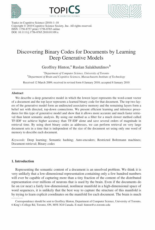
and positive for others. Fig. 2 shows that this is what the fine-tuning does. We tried other

ways of encouraging the code units to be binary, but Gaussian noise worked better.

To prevent the added Gaussian noise from messing up the conjugate gradient fine-tuning,

we used ‘‘deterministic noise’’ with mean zero and variance 16. For each training case, the

sampled noise values are fixed in advance and do not change during training. With a limited

number of training cases, the optimization could tailor the parameters to the fixed noise val-

ues, but this is not possible when the total number of sampled noise values is much larger

than the number of parameters.

4.3. Details of the training

To speedup the pretraining, we subdivided both datasets into small mini-batches, each

containing 100 cases,1 and updated the weights after computing the gradient of the recon-

struction error on each mini-batch. For large datasets this is much more efficient than using

the entire dataset to compute the gradient. Early in the training, the gradient vector com-

puted from a small mini-batch is likely to point in the same general direction as the gradient

vector computed from the whole dataset, so progress can be made rapidly by just using one

0 0.2 0.4 0.6 0.8 10

1

2

3

4

5

6

7x 10

5B

0 0.2 0.4 0.6 0.8 10

0.5

1

1.5

2

2.5x 10

5A

Fig. 2. The distribution of the activities of the 128-code units on the 20 Newsgroup training data before and after

adding deterministic noise to the code units. When the fine-tuning of the autoencoder network is performed with-

out adding noise, the code layer learns to transmit a lot of information by using precise real values that lie

between 0 and 1. The distribution of values is shown on the left. If these values are thresholded to produce a bin-

ary code, the reconstruction will be poor because the fine-tuning did not take the thresholding into account. If

additional noise is added to the input to the code units during the fine-tuning, the total input received from the

layer below learns to be big and positive or big and negative so that the code unit can still transmit one bit of

information despite the noise. This distribution is shown on the right and it makes the codes much more robust

to thresholding.


small mini-batch per weight update. Of course, there will be sampling noise when the gradi-

ent is computed in this way, but that will be corrected on subsequent mini-batches.

For both datasets each layer was greedily pretrained for 50 passes (epochs) through the

entire training dataset. The weights were updated using a learning rate of 0.1, momentum of

0.9, and a weight decay of 0.0002 · weight · learning rate. The weights were initialized

with small random values sampled from a zero-mean normal distribution with variance

0.01.

For fine-tuning we used the method of conjugate gradients2 on larger minibatches of

1,000 data vectors, with three line searches performed for each minibatch in each epoch.

To determine an adequate number of epochs and to avoid overfitting, we fine-tuned on a

fraction of the training data and tested performance on the remaining validation data. We

then repeated fine-tuning on the entire training dataset for 50 epochs. Slight overfitting

was observed on the 20 Newsgroup corpus but not on the Reuters corpus. After fine-tun-

ing the codes were thresholded to produce binary code vectors. The asymmetry between

0 and 1 in the energy function of an RBM causes the unthresholded codes to have many

more values near 0 than near 1, so we used a threshold of s ¼ 0.1. This works well for

document retrieval even though it is suboptimal for document reconstruction.

We experimented with various values for the noise variance and the threshold, as well as

the learning rate, momentum, and weight-decay parameters used in the pretraining. Our

results are fairly robust to variations in these parameters and also to variations in the number

of layers and the number of units in each layer. The precise weights found by the pretraining

do not matter as long as it finds a good region from which to start the fine-tuning (Erhan,

Manzagol, Bengio, Bengio, & Vincent, 2009).

5. Experimental results

To evaluate performance of our model on an information retrieval task we do the following:

Document retrieval procedure:

1. Map all query (test) documents into 128-bit binary codes by performing an up-pass

through the model and thresholding top-level activation probabilities at s ¼ 0.1.

2. For each query document:

Calculate its similarity to all other test documents in the 128-bit space using Hamming

distance.

Retrieve the D most similar documents.

Measure accuracy by computing the ratio of correctly retrieved documents (which

belong to the same category as a query document) to the total number of retrieved doc-

uments.

3. Average results across all queries.

Results of Gehler et al. (2006) show that pLSA and LDA models do not generally

outperform LSA and TF-IDF. Therefore, for comparison, we only used LSA and TF-IDF as


benchmark methods. For LSA each word count, ci, was replaced by log (1 + ci) before the

SVD, which slightly improved performance. TF-IDF computes document similarity directly

in the word-count space, which is slow. For both these methods we used the cosine of the

angle between two vectors as a measure of their similarity.

‘‘TF-IDF’’ stands for ‘‘Term-Frequency, Inverse-Document-Frequency’’ and it is a very

sensible way of deciding how important the counts of a particular word-type are for deter-

mining the similarity of two documents. If a particular word has a high count (a high Term

Frequency) in both documents this makes them similar. But the similarity is much greater if

that word is rare in documents in general (a high Inverse Document Frequency). Generally,

the logarithm of the inverse document frequency is used.

5.1. Description of the text corpora

In this section we present experimental results for document retrieval on two text data-

sets: 20-Newsgroups and Reuters Corpus Volume II.

The 20 newsgroup corpus contains 18,845 postings taken from the Usenet newsgroup

collection. The corpus is partitioned fairly evenly into 20 different newsgroups, each cor-

responding to a separate topic.3 The data were split by date into 11,314 training and

7,531 test articles, so the training and test sets were separated in time. The training set

was further randomly split into 8,314 training and 3,000 validation documents. Some

newsgroups are very closely related to each other, for example, soc.religion.christian and

talk.religion.misc, while others are very different, for example, rec.sport.hockey and

comp.graphics (see Fig. 3).

We further preprocessed the data by removing common stopwords, stemming, and then

only considering the 2,000 most frequent words in the training dataset. As a result, each

posting was represented as a vector containing 2,000 word counts. No other preprocessing

was made.

The Reuters Corpus Volume II is an archive of 804,414 newswire stories4 that have

been manually categorized into 103 topics. The corpus covers four major groups: corpo-

rate/industrial, economics, government/social, and markets. Sample topics are displayed in

Fig. 3. The data were randomly split into 402,207 training and 402,207 test articles. The

training set was further randomly split into 302,207 training and 100,000 validation docu-

ments. The available data were already in the preprocessed format, where common stop-

words were removed and all documents were stemmed. We again only considered the

2,000 most frequent words in the training dataset.

5.2. Results

For both datasets we used the 2000-500-500-128 architecture shown in Fig. 1. To see

whether the learned 128-bit codes preserve class information, we used Stochastic Neighbor

Embedding (Hinton & Roweis, 2003) to visualize the 128-bit codes of all the documents

from five or six separate classes. Fig. 3 shows that for both datasets the 128-bit codes

preserve the class structure of the documents.


In addition to requiring very little memory, binary codes allow very fast search because

fast bit counting routines5 can be used to compute the Hamming distance between two bin-

ary codes. On a 3GHz Intel Xeon running C, for example, it only takes 3.6 ms to search

through 1 million documents using 128-bit codes. The same search takes 72 ms for 128-

dimensional LSA and 1.2 s for TF-IDF, though this could be considerably reduced by using

a less naive method that uses inverted indexing.

20 Newsgroup 2−D Topic Space

comp.graphics

rec.sport.hockey

sci.cryptography

soc.religion.christian

talk.politics.guns

talk.politics.mideast

Reuters 2−D Topic Space

Accounts/Earnings

Government Borrowing

European Community Monetary/Economic

Disasters and Accidents

Energy Markets

A

B

Fig. 3. Two-dimensional embedding of 128-bit codes using SNE for 20 Newsgroup data (panel A) and Reuters

RCV2 corpus (panel B).


1 3 7 15 31 63 127 255 511 1023 2047 4095 75310

0.1

0.2

0.3

0.4

0.5

0.6

0.7

0.8

0.9

128−bit DGM prior to fine−tuning

Fine−tuned 128−bit DGM

LSA 128

Newsgroup Dataset

Number of Retrieved Documents

Acc

urac

y

1 3 7 15 31 63 127 255 511 1023 2047 4095 75310

0.1

0.2

0.3

0.4

0.5

0.6

0.7

0.8

0.9

TF−IDF

Hybrid 128−bit DGMusing TF−IDF

LSA 128

Newsgroup Dataset


Acc

urac

yA

B

Fig. 4. Accuracy curves for 20 Newsgroup dataset, when a query document from the test set is used to retrieve

other test set documents, averaged over all 7,531 possible queries.


Figs. 4 and 5 (panels A) show that our 128-bit codes are better at document retrieval than

the 128 real-values produced by LSA. TF-IDF is slightly more accurate than our 128-bit

codes6 when retrieving the top 15–30 documents in either dataset. If, however, we use our

128-bit codes to preselect the top 100 documents for the 20 Newsgroup data or the top

1,000 for the Reuters data, and then re-rank these preselected documents using TF-IDF, we

get better accuracy than running TF-IDF alone on the whole document set (see Figs. 4

and 5). This shows that the 128-bit codes can correctly reject some documents that TF-IDF

would rank very highly. On 400,000 documents, the naive implementation of TF-IDF

takes 0.48 s and our more accurate hybrid method takes .0014 + .0012 s—about 200 times

faster.

1 3 7 15 31 63 127 255 511 10230.2

0.25

0.3

0.35

0.4

0.45

0.5

0.55

128−bit DGM prior to fine−tuning

Fine−tuned 128−bit DGM

LSA 128

Reuters Corpus


Acc

urac

y

1 3 7 15 31 63 127 255 511 10230.2

0.25

0.3

0.35

0.4

0.45

0.5

0.55

TF−IDF

Hybrid 128−bit DGM using TF−IDF

LSA 128

Reuters Corpus


Acc

urac

y

A

B

Fig. 5. Accuracy curves for Reuters RCV2 dataset, when a query document from the test set is used to retrieve

other test set documents, averaged over all 402,207 possible queries.


6. Retrieval in constant time using a semantic address space

Using 128-bit codes, we have shown that documents which are semantically similar can

be mapped to binary vectors that are close in hamming space. If we could do this for 30-bit

codes, we would have the ultimate retrieval method: Given a query document, compute its

30-bit address and retrieve all of the documents stored at similar addresses with no search at

all. For a billion documents, a 30-bit address space gives a density of one document per

address and a hamming-ball of radius 5 should contain about 175,000 documents. The

retrieved documents could then be given to a slower but more precise retrieval method. It is

unlikely that the 175,000 documents in the hamming-ball would contain most of the very

similar documents, so recall would not be high, but it is possible that precision could still be

very good.

Using 20-bit codes, we checked whether our learning procedure could discover a way to

model similarity of count-vectors by similarity of 20-bit addresses that was good enough to

allow high precision retrieval for our set of 402,207 test documents. For example, a ham-

ming ball of radius 4 contains 6,196 of the million addresses so it should contain about

2,500 documents. Fig. 6 shows that accuracy is not lost by restricting TF-IDF to this pres-

elected set. We can also use a two-stage filtering procedure by first retrieving documents

using 20-bit addresses in a hamming ball of larger radius 6 (about 25,000 documents), filter

these down to 1,000 using 128-bit codes, and then apply TF-IDF. This method is faster and

achieves higher accuracy as shown in Fig. 6.

Scaling up the learning to a billion training cases would not be particularly difficult.

Using mini-batches, the learning time is sublinear in the size of the dataset if there is

0.1 0.2 0.4 0.8 1.6 3.2 6.4 12.8 25.6 51.2 100 0

10

20

30

40

50

Recall (%)

Pre

cisi

on

(%

)

TF−IDFTF−IDF using 20 bitsTF−IDF using 20 bitsand 128 bitsLocally Sensitive Hashing

Fig. 6. Accuracy curves for Reuters RCV2 dataset, when a query document from the test set is used to retrieve

other test set documents, averaged over all 402,207 possible queries. Locality sensitive hashing (LSH) is the

fastest current method for finding similar documents. It is less accurate and also much slower than using

the Hamming ball around a learned binary code to create a shortlist for TF-IDF.


redundancy in the data as there surely is. Also, different processors can be used to com-

pute the gradients for different examples within a large mini-batch. To improve recall,

we could learn several different ‘‘semantic’’ address spaces on disjoint training sets and

then preselect documents that are close to the query document in any of the semantic

address spaces.

7. Discussion

We have described a rather complicated way of learning efficient, compact, nonlinear

codes for documents, and we have shown that these codes are very good for retrieving simi-

lar documents. The learning is slow, especially the fine-tuning stage, but it scales very well

with the size of the dataset. The use of a simple gradient method as opposed to a compli-

cated convex optimization, means that it is easy to incorporate new data without starting all

over again. Even though the learning is quite slow, the inference is very fast. The code for a

new document can be extracted by a single, deterministic feed-forward pass through the

encoder part of the network and this requires only a few vector-matrix multiplies.

To gain further insight into the nature of the codes that are learned, it would be helpful if

we could visualize what the individual elements of the codes represent. Unfortunately, this

is not nearly as easy to do as with topic models because in our codes, each component is

activated by a very large set of documents and the precision comes by intersecting all of

these sets. By contrast, in topic models each word must be generated by a single topic so the

individual topics are, necessarily, far more precise and therefore far easier to visualize. For

generative models of labeled data it is possible to fix the class label and see what typical

instances of that class look like as is done in Hinton et al. (2006), but this method cannot be

applied when the model is learned on unlabeled data.

Our method for learning codes could be applied to the same word document matrix in a

different way by treating each word as a training case rather than each document. The codes

would then represent word meanings and it would be interesting to visualize them in a

two-dimensional map using t-SNE (van der Maaten & Hinton, 2008), which is very good at

organizing the layout so that very similar codes are very close to one another (see http://

www.cs.toronto.edu/ hinton/turian.png for an example).

While the use of short codes may be interesting for the technology of information retrie-

val, we think it is largely irrelevant to the issue of how people represent and retrieve docu-

ments for the reasons given in the Introduction. However, the same deep learning methods

can be used to extract very large, very sparse codes, and we think this is a far more promis-

ing direction for future research on how the brain represents the contents of a document.

Notes

1. The last minibatch contained more than 100 cases.

2. Code is available at http://www.kyb.tuebingen.mpg.de/bs/people/carl/code/minimize/.


3. The data are available at http://people.csail.mit.edu/jrennie/20Newsgroups (20news-

bydate.tar.gz). It has been preprocessed and organized by date.

4. The Reuter Corpus Volume 2 is available at http://trec.nist.gov/data/reuters/

reuters.html.

5. Code is available at http://www-db.stanford.edu/�manku/bitcount/bitcount.html.

6. 256-bit codes work slightly better that 128-bit ones.

Acknowledgments

This research was supported by NSERC, CFI, and Google. G. E. H. is a fellow of the

Canadian Institute for Advanced Research.

References

Blei, D. M., Ng, A. Y., & Jordan, M. I. (2003). Latent dirichlet allocation. Journal of Machine LearningResearch, 3, 993–1022.

Deerwester, S. C., Dumais, S. T., Landauer, T. K., Furnas, G. W., & Harshman, R. A. (1990). Indexing by latent

semantic analysis. Journal of the American Society of Information Science, 41(6), 391–407.

Erhan, D., Manzagol, P., Bengio, Y., Bengio, S., & Vincent, P. (2009). The difficulty of training deep

architectures and the effect of unsupervised pre-training. AISTATS 2009, 5, 153–160.

Gehler, P., Holub, A., & Welling, M. (2006). The rate adapting poisson (RAP) model for information retrieval

and object recognition. Proceedings of the 23rd International Conference on Machine Learning. Pittsburgh,

PA.

Hinton, G. E. (2002). Training products of experts by minimizing contrastive divergence. Neural Computation,

14(8), 1711–1800.

Hinton, G. E. (2007a). Learning multiple layers of representation. Trends in Cognitive Science, 11, 428–434.

Hinton, G. E. (2007b). To recognize shapes, first learn to generate images. In P. Cisek, D. Kalaska, & J. Haran

(Eds.), Computational neuroscience: Theoretical insights into brain function (pp. 535–547). Montreal:

Elsevier.

Hinton, G. E., & Roweis, S. T. (2003). Stochastic neighbor embedding. In S. Thrun, L. K. Saul, & B. Scholkopf

(Eds.), Advances in neural information processing systems 15 (pp. 833–840). Cambridge, MA: MIT Press.

Hinton, G. E., & Salakhutdinov, R. R. (2006). Non-linear dimensionality reduction using neural networks.

Science, 313, 504–507.

Hinton, G. E., & Sejnowski, T. J. (1983). Optimal perceptual inference. In Proceedings of the IEEE conferenceon computer vision and pattern recognition, Washington, DC.

Hinton, G. E., McClelland, J. L., & Rumelhart, D. E. (1986). Distributed representations. In D. E. Rumelhart &

J. L. McClelland (Eds.), Parallel distributed processing: explorations in the microstructure of cognition.Volume 1: Foundations (pp. 77–109). Cambridge, MA: MIT Press.

Hinton, G. E., Osindero, S., & Teh, Y. W. (2006). A fast learning algorithm for deep belief nets. NeuralComputation, 18, 1527–1554.

Hofmann, T. (1999). Probabilistic latent semantic analysis. In P. Laskey & H. Prade (Eds.), Proceedings of the15th conference on uncertainty in AI (pp. 286–296). Stockholm, Sweden: Morgan Kaufmann.

Jordan, M. (1999). Learning in Graphical Models. Cambridge, MA: MIT Press.

van der Maaten, L. J. P., & Hinton, G. E. (2008). Visualizing data using t-sne. Journal of Machine LearningResearch, 9, 2579–2605.


Pearl, J. (1988). Probabilistic inference in intelligent systems: networks of plausible inference. San Mateo, CA:

Morgan Kaufmann.

Salakhutdinov, R. R., & Hinton, G. E. (2007). Semantic hashing. In J. Fernandez-Luna, B. Piwowarski, & J. F.

Huete (Eds.), Proceedings of the SIGIR Workshop on Information Retrieval and Applications of GraphicalModels). Amsterdam, The Netherlands.

Salton, G., & Buckley, C. (1988). Term-weighting approaches in automatic text retrieval. InformationProcessing and Management, 24(5), 513–523.

Welling, M., Rosen-Zvi, M., & Hinton, G. (2005). Exponential family harmoniums with an application to

information retrieval. In L. Saul, Y. Weiss, & L. Bottou (Eds.), Advances in neural information processingsystems 17 (pp. 1481–1488). Cambridge, MA: MIT Press.

Xing, E., Yan, R., & Hauptmann, A. G. (2005). Mining associated text and images with dual-wing harmoniums.

In F. Baccus, & T. Jaakkola (Eds.), Proceedings of the 21st conference on uncertainty in artificial intelli-gence (pp. 633–641). Edinburgh, Scotland: AUAI press.
