Discontinuous Galerkin Methods for Solving Euler Equations

Andrey Andreyev (andreyev@umd.edu)

Adviser: James Baeder (baeder@umd.edu)

Final PresentationMay 7, 2013

Motivation

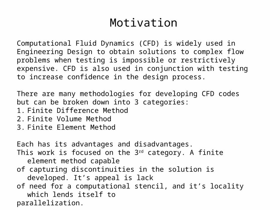
Computational Fluid Dynamics (CFD) is widely used in Engineering Design to obtain solutions to complex flow problems when testing is impossible or restrictively expensive. CFD is also used in conjunction with testing to increase confidence in the design process.

There are many methodologies for developing CFD codes but can be broken down into 3 categories:1. Finite Difference Method2. Finite Volume Method3. Finite Element Method

Each has its advantages and disadvantages.This work is focused on the 3rd category. A finite element method capable of capturing discontinuities in the solution is developed. It’s appeal is lackof need for a computational stencil, and it’s locality which lends itself to parallelization.

Objectives:

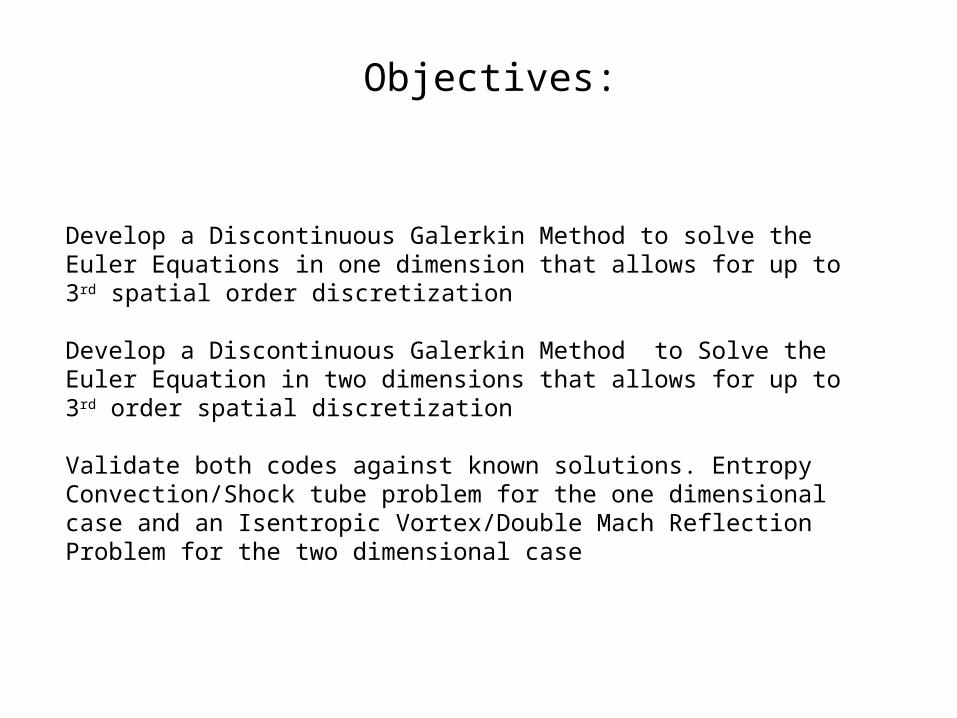
Develop a Discontinuous Galerkin Method to solve the Euler Equations in one dimension that allows for up to 3rd spatial order discretization

Develop a Discontinuous Galerkin Method to Solve the Euler Equation in two dimensions that allows for up to 3rd order spatial discretization

Validate both codes against known solutions. Entropy Convection/Shock tube problem for the one dimensional case and an Isentropic Vortex/Double Mach Reflection Problem for the two dimensional case

Outline of Presentation

• Euler Equation description• Overview of Current Numerical Methods in CFD

-Spatial Discretization Overview-Overview of Conservative Methods-Riemann Problem • Description of General Discontinuous Galerkin Method-Slope Limiting of DG method for stability-Time Stepping using 3rd order Runge Kutta• 1D Problem Description-Results/Validation

• 2D Problem Description -2D Results/Validation

• Summary• Review of Schedule• Description of deliverables

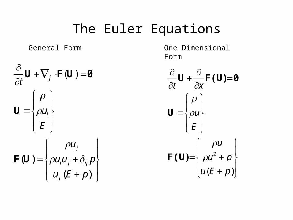
The Euler Equations

)(

)(

)(

pEu

puu

u

E

u

t

j

ijji

j

i

j

UF

U

0UFU

General Form

)(

2

pEu

pu

u

E

u

xt

F(U)

U

0F(U)U

One Dimensional Form

Overview of Current Computational Approaches

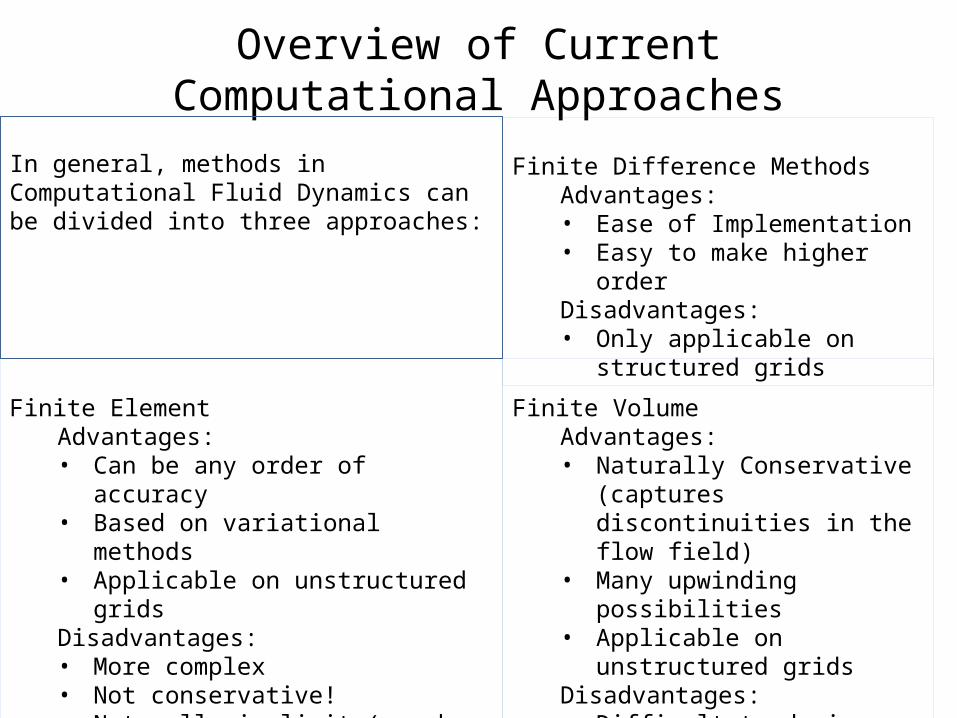
Finite Difference MethodsAdvantages: • Ease of Implementation • Easy to make higher orderDisadvantages:• Only applicable on structured

grids

Finite VolumeAdvantages: • Naturally Conservative (captures

discontinuities in the flow field)• Many upwinding possibilities• Applicable on unstructured gridsDisadvantages:• Difficult to devise stable higher

order scheme

Finite ElementAdvantages: • Can be any order of accuracy• Based on variational methods• Applicable on unstructured gridsDisadvantages:• More complex• Not conservative!• Naturally implicit (can be explicit with

modifications)

In general, methods in Computational Fluid Dynamics can be divided into three approaches:

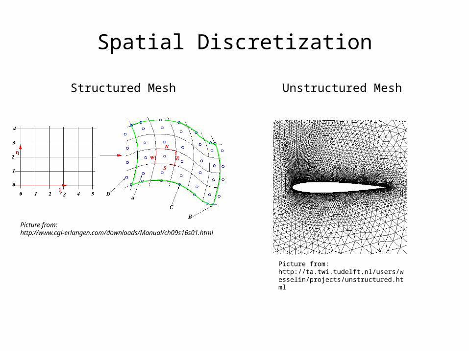
Spatial Discretization

Picture from: http://www.cgl-erlangen.com/downloads/Manual/ch09s16s01.html

Structured Mesh Unstructured Mesh

Picture from: http://ta.twi.tudelft.nl/users/wesselin/projects/unstructured.html

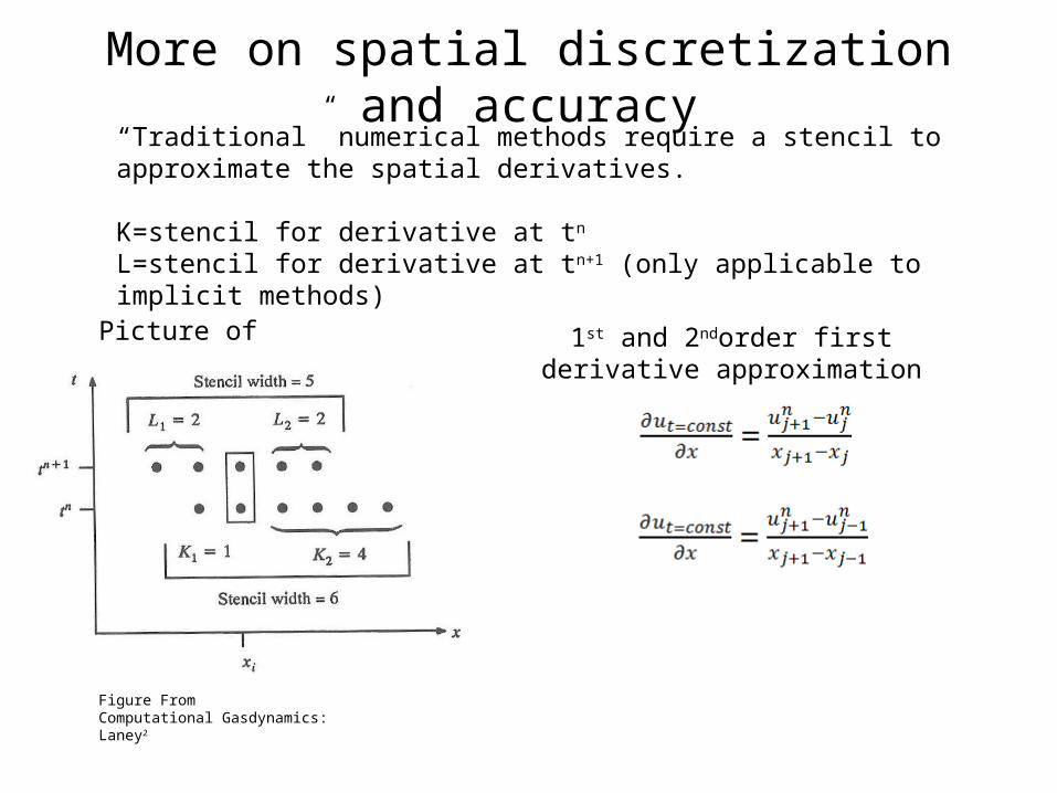
More on spatial discretization and accuracy

Picture of stencil 1st and 2ndorder first derivative approximation

Figure FromComputational Gasdynamics: Laney2

“Traditional” numerical methods require a stencil to approximate the spatial derivatives.

K=stencil for derivative at tn L=stencil for derivative at tn+1 (only applicable to implicit methods)

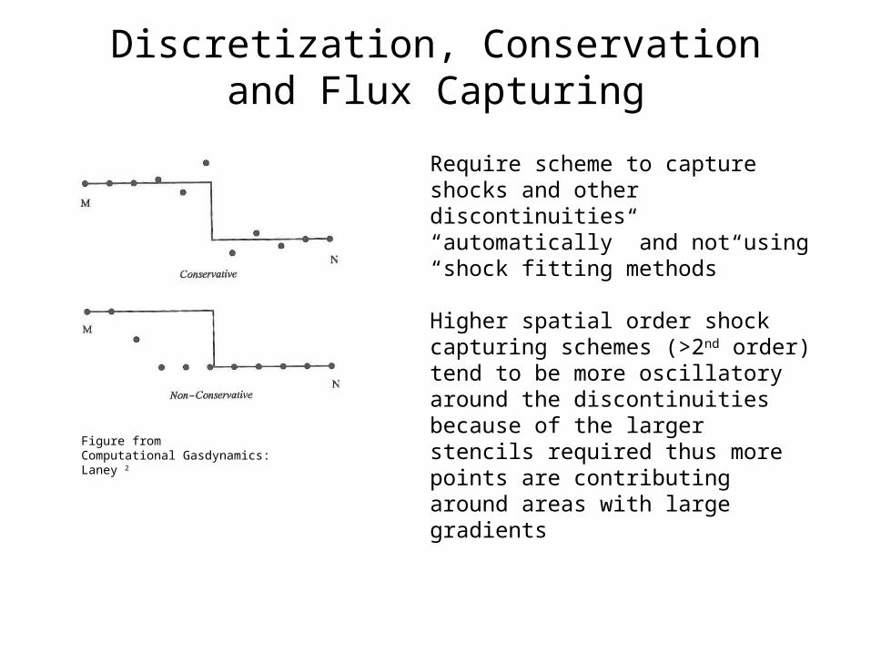
Discretization, Conservation and Flux Capturing

Figure fromComputational Gasdynamics: Laney 2

Require scheme to capture shocks and other discontinuities “automatically” and not using “shock fitting methods”

Higher spatial order shock capturing schemes (>2nd order) tend to be more oscillatory around the discontinuities because of the larger stencils required thus more points are contributing around areas with large gradients

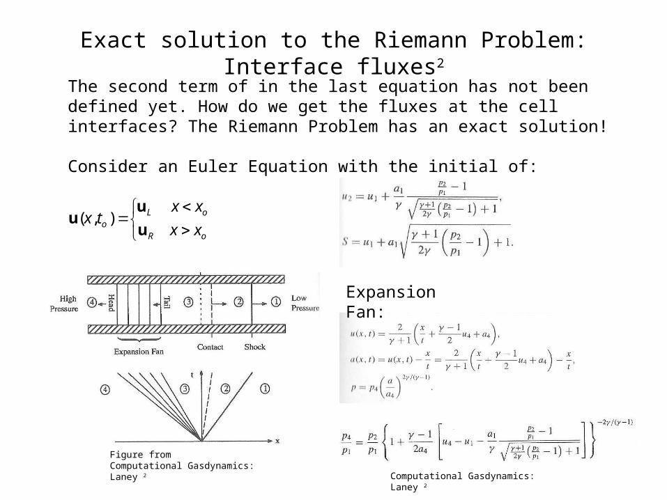
Exact solution to the Riemann Problem: Interface fluxes2

The second term of in the last equation has not been defined yet. How do we get the fluxes at the cell interfaces? The Riemann Problem has an exact solution!

Consider an Euler Equation with the initial of:

oR

oLo xx

xxtx

u

uu ),(

Expansion Fan:

Figure fromComputational Gasdynamics: Laney 2

Computational Gasdynamics: Laney 2

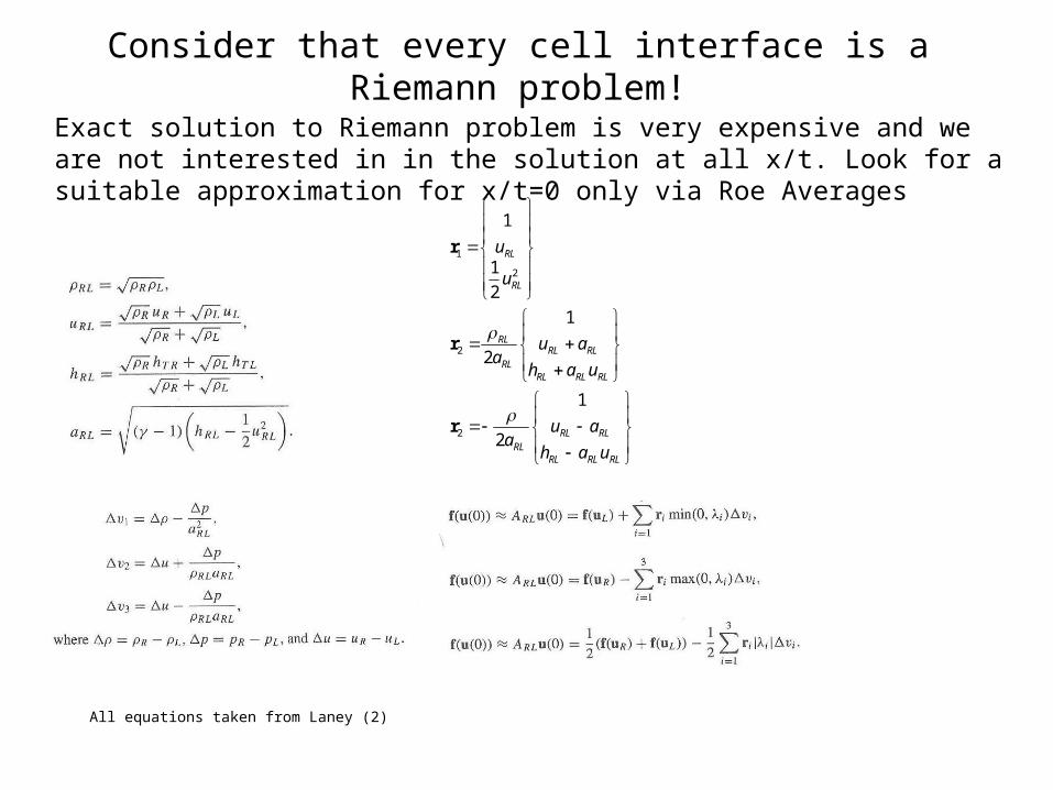
Consider that every cell interface is a Riemann problem!

Exact solution to Riemann problem is very expensive and we are not interested in in the solution at all x/t. Look for a suitable approximation for x/t=0 only via Roe Averages

RLRLRL

RLRLRL

RLRLRL

RLRLRL

RL

RL

RL

uah

aua

uah

aua

u

u

1

2

1

2

2

1

1

2

2

2

1

r

r

r

All equations taken from Laney (2)

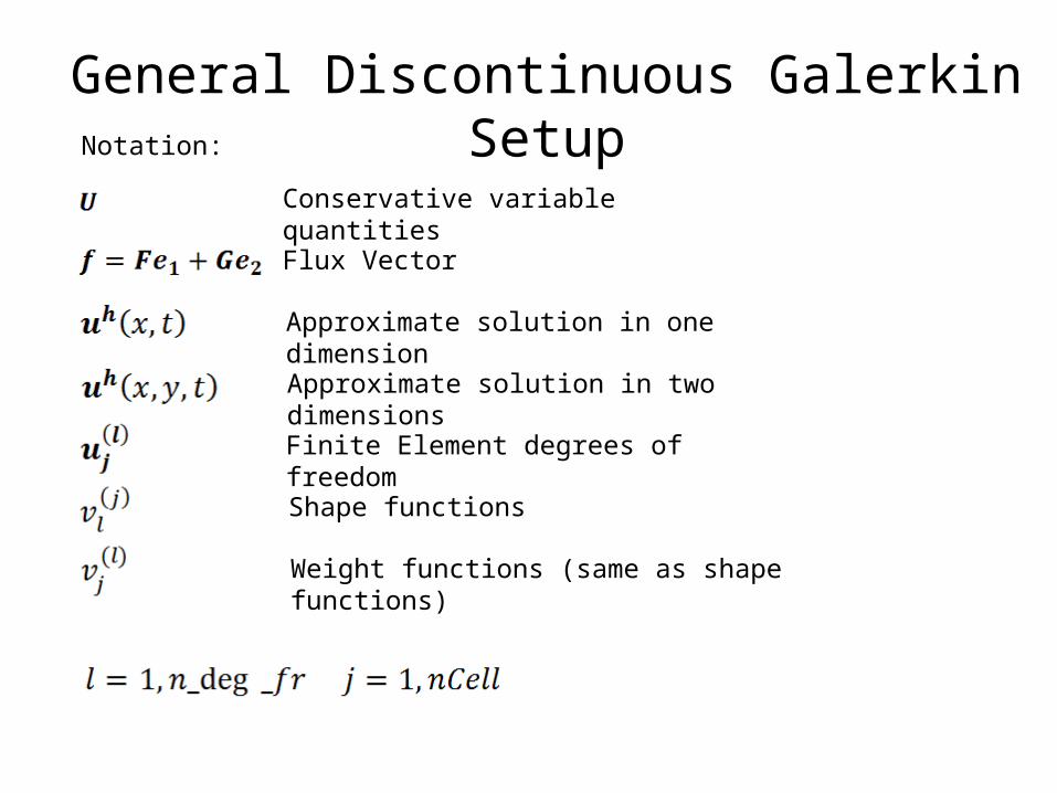
Notation:

General Discontinuous Galerkin Setup

Conservative variable quantities

Flux Vector

Approximate solution in one dimension

Approximate solution in two dimensions

Finite Element degrees of freedom

Shape functions

Weight functions (same as shape functions)

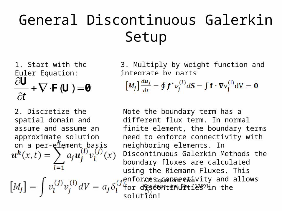
1. Start with the Euler Equation:

0UFU

)(t

2. Discretize the spatial domain and assume and assume an approximate solution on a per-element basis

3. Multiply by weight function and integrate by parts

Note the boundary term has a different flux term. In normal finite element, the boundary terms need to enforce connectivity with neighboring elements. In Discontinuous Galerkin Methods the boundary fluxes are calculated using the Riemann Fluxes. This enforces connectivity and allows for discontinuities in the solution!

General Discontinuous Galerkin Setup

All Equations from Cockburn and Shu [1989] (1)

One-Dimensional Discontinuous Galerkin1

)(

2

pEu

pu

u

E

u

xt

F(U)

U

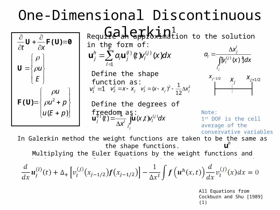
0F(U)URequire an approximation to the solution in the form of:

k

l

jl

ljl

hj dxxvta

1

)()( )()(uu

11 jv jj xxv 2

222 12

1)( jj

j xxxv

jI

jll

lj dxvtx

xt )()( ),(

1)( uu

jI

jl

lj

ldxxv

xa

2)( )]([

Define the degrees of freedom as:

Define the shape function as:

Note:1st DOF is the cell average of the conservative variables

In Galerkin method the weight functions are taken to be the same as the shape functions.Multiplying the Euler Equations by the weight functions and substituting for U and

integrating by parts, we obtain the following form:

hu

All Equations from Cockburn and Shu [1989] (1)

2/1jx2/1jxjx

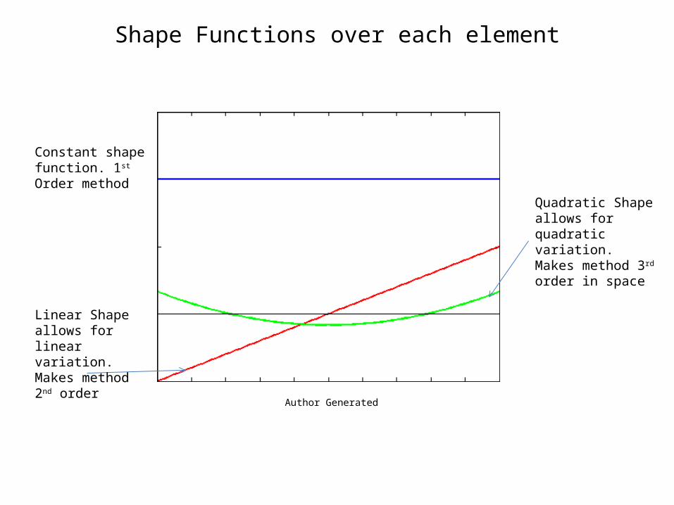
Shape Functions over each element

Author Generated

Linear Shape allows for linear variation. Makes method 2nd order

Quadratic Shape allows for quadratic variation. Makes method 3rd order in space

Constant shape function. 1st Order method

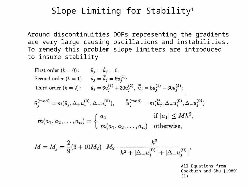
Slope Limiting for Stability1

Around discontinuities DOFs representing the gradients are very large causing oscillations and instabilities. To remedy this problem slope limiters are introduced to insure stability

All Equations from Cockburn and Shu [1989] (1)

Runge-Kutta Time Explicit Time Marching

• Time integration of the equations will be carried out using a higher order Runge-Kutta technique.

• The space discretization in the previous slide converted the PDEs into a system of ODEs in time.

• Using Higher Order Runge-Kutta, we carry out the time integration on a per-element basis

jj

j

au

xCFLt min

Note:Time Step is calculated based on the largest Eigenvalue i.e. fastest information transfer

All Equations from Cockburn and Shu [1989] (1)

DG Method Approach

)(

2

pEu

pu

u

E

u

xt

F(U)

U

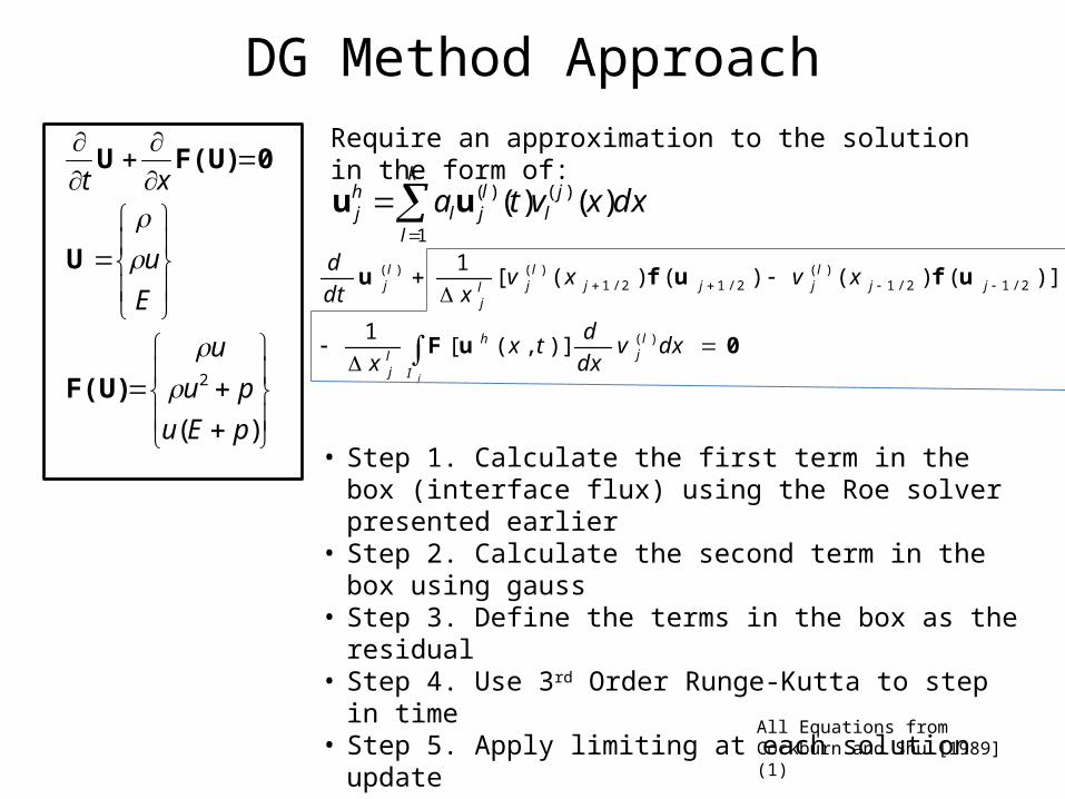
0F(U)URequire an approximation to the solution in the form of:

k

l

jl

ljl

hj dxxvta

1

)()( )()(uu

0uF

ufufu

jI

lj

hlj

jjl

jjjl

jlj

lj

dxvdx

dtx

x

xvxvxdt

d

)(

2/12/1)(

2/12/1)()(

)],([1

)]()()()([1

All Equations from Cockburn and Shu [1989] (1)

• Step 1. Calculate the first term in the box (interface flux) using the Roe solver presented earlier

• Step 2. Calculate the second term in the box using gauss• Step 3. Define the terms in the box as the residual • Step 4. Use 3rd Order Runge-Kutta to step in time• Step 5. Apply limiting at each solution update

DG Method 1DTest Problems

The method was tested on 3 problems1. Entropy Convection Problem(Smooth solution, requires no limiting) used for validation2. Sod’s Shock Tube Problem (Simple discontinuous solution, has analytical solution)3. Osher’s Problem (Discontinuous Solution with complex flow structures, no analytical

solution)

Testing 1D With no Limiter

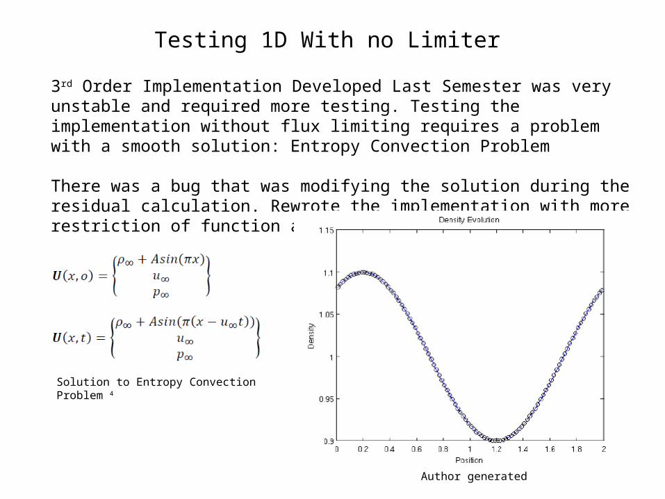
3rd Order Implementation Developed Last Semester was very unstable and required more testing. Testing the implementation without flux limiting requires a problem with a smooth solution: Entropy Convection Problem

There was a bug that was modifying the solution during the residual calculation. Rewrote the implementation with more restriction of function access

Solution to Entropy Convection Problem 4

Author generated

Density Evolution

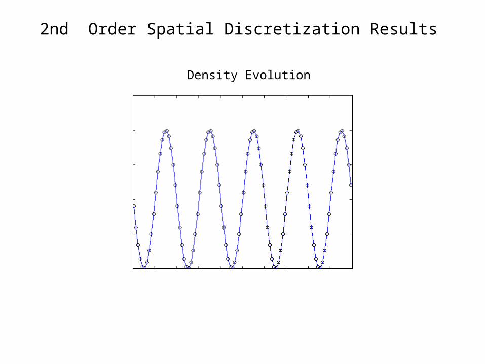
2nd Order Spatial Discretization Results

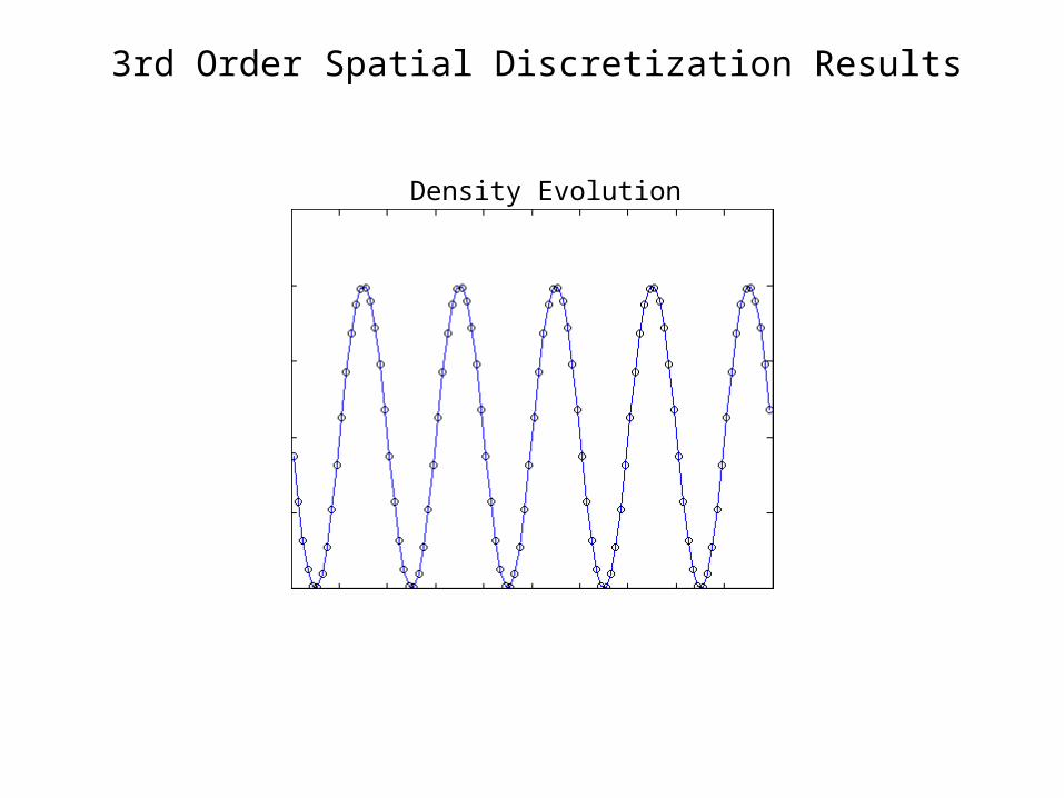
3rd Order Spatial Discretization Results

Density Evolution

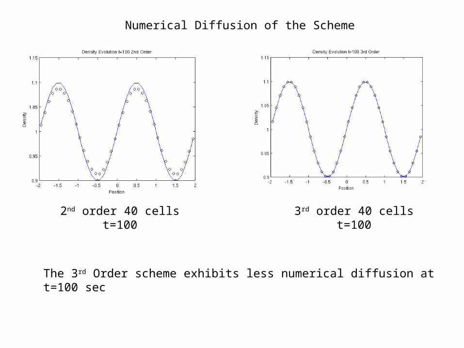
Numerical Diffusion of the Scheme

The 3rd Order scheme exhibits less numerical diffusion at t=100 sec

2nd order 40 cells t=100 3rd order 40 cells t=100

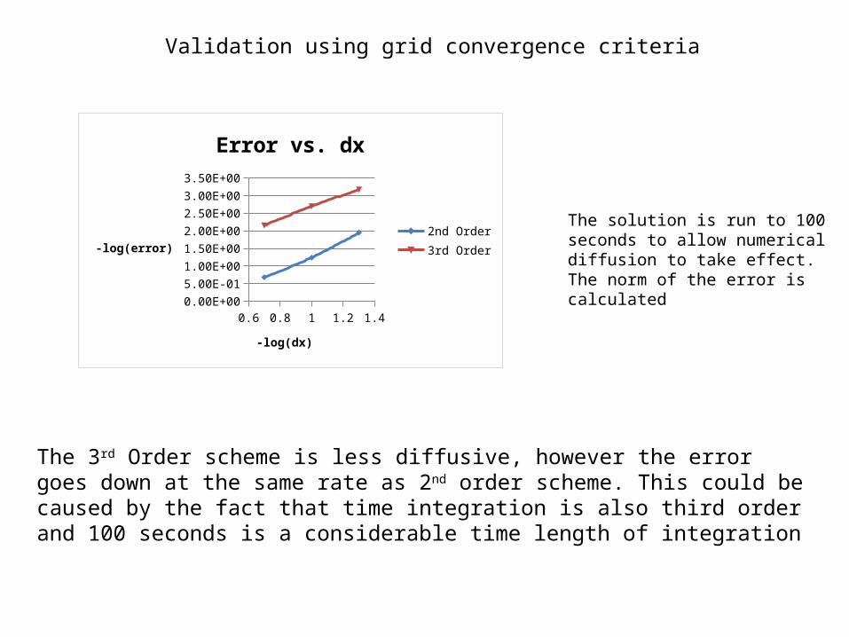
Validation using grid convergence criteria

The 3rd Order scheme is less diffusive, however the error goes down at the same rate as 2nd order scheme. This could be caused by the fact that time integration is also third order and 100 seconds is a considerable time length of integration

The solution is run to 100 seconds to allow numerical diffusion to take effect. The norm of the error is calculated

0.6 0.7 0.8 0.9 1 1.1 1.2 1.3 1.40.00E+00

5.00E-01

1.00E+00

1.50E+00

2.00E+00

2.50E+00

3.00E+00

3.50E+00

Error vs. dx

2nd Order3rd Order

-log(dx)

-log(error)

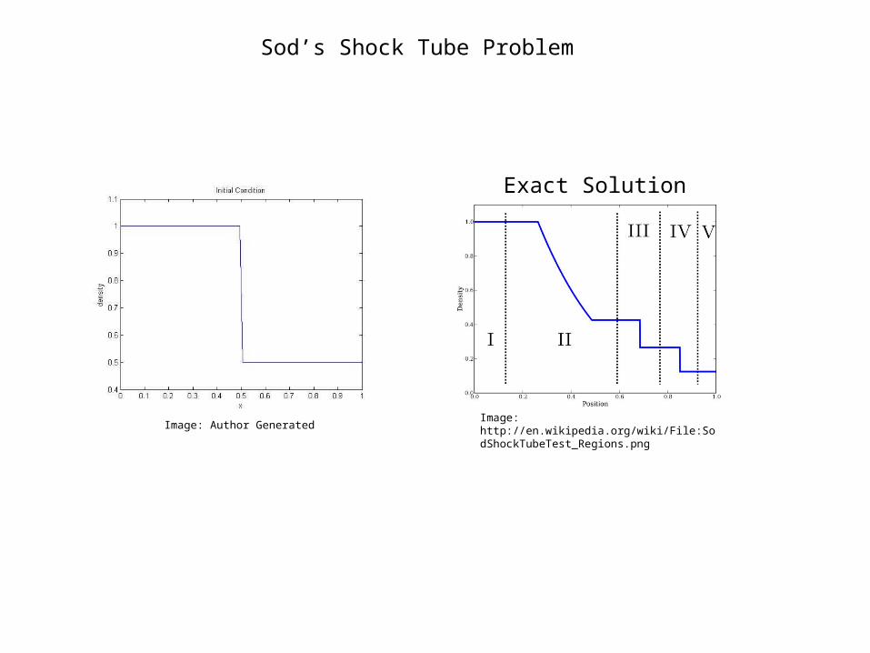
Image: http://en.wikipedia.org/wiki/File:SodShockTubeTest_Regions.png

Exact Solution

Image: Author Generated

Sod’s Shock Tube Problem

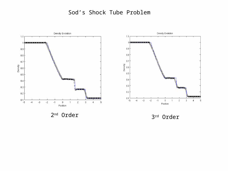
Sod’s Shock Tube Problem

2nd Order 3rd Order

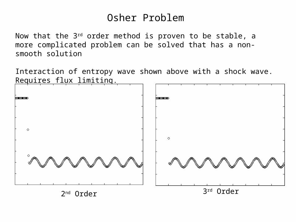
Osher Problem

Now that the 3rd order method is proven to be stable, a more complicated problem can be solved that has a non-smooth solution

Interaction of entropy wave shown above with a shock wave. Requires flux limiting.

2nd Order 3rd Order

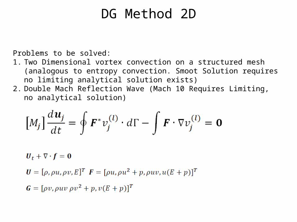
DG Method 2D

Problems to be solved:1. Two Dimensional vortex convection on a structured mesh (analogous to entropy

convection. Smoot Solution requires no limiting analytical solution exists)2. Double Mach Reflection Wave (Mach 10 Requires Limiting, no analytical solution)

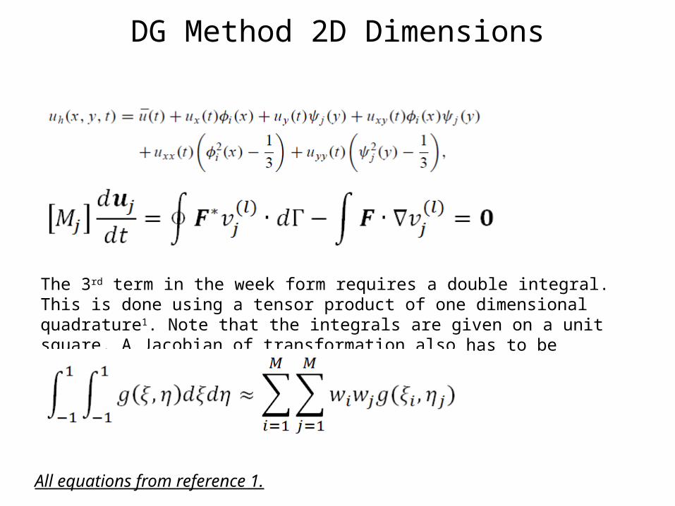
DG Method 2D Dimensions

The 3rd term in the week form requires a double integral. This is done using a tensor product of one dimensional quadrature1. Note that the integrals are given on a unit square. A Jacobian of transformation also has to be calculated.

All equations from reference 1.

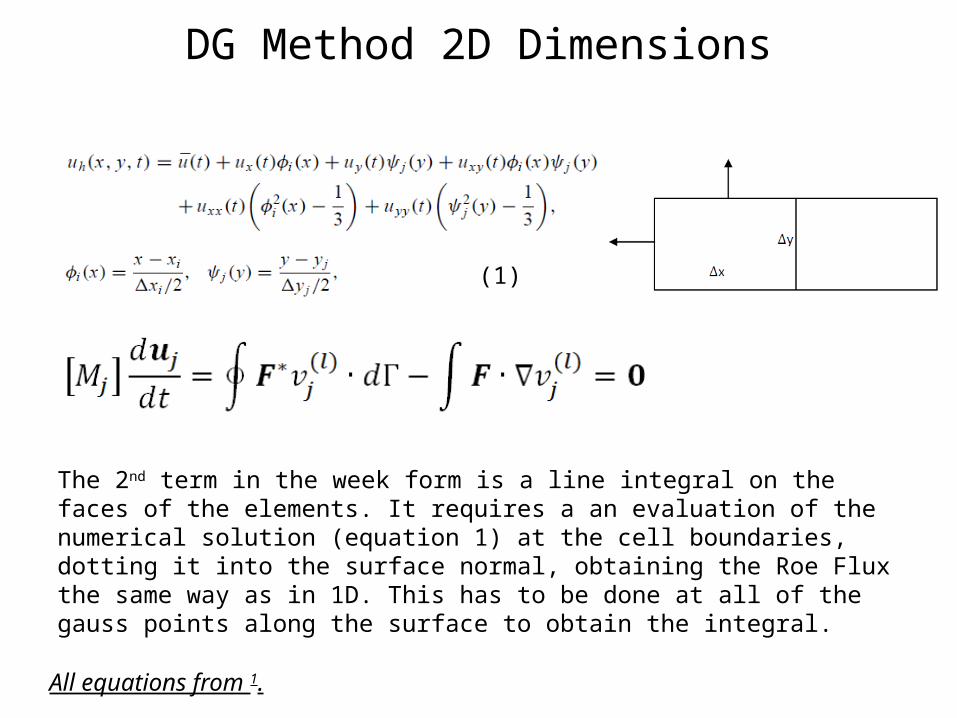
DG Method 2D Dimensions

The 2nd term in the week form is a line integral on the faces of the elements. It requires a an evaluation of the numerical solution (equation 1) at the cell boundaries, dotting it into the surface normal, obtaining the Roe Flux the same way as in 1D. This has to be done at all of the gauss points along the surface to obtain the integral.

All equations from 1.

(1)

DG Method 2D Dimensions: IsentropicVortex Convection

All equations and images from reference 4.

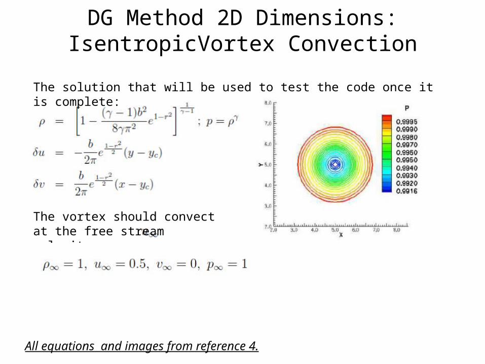
The solution that will be used to test the code once it is complete:

The vortex should convect at the free stream velocity .

Isentropic Vortex Solution

2D Validation

All equations and images from reference 4.

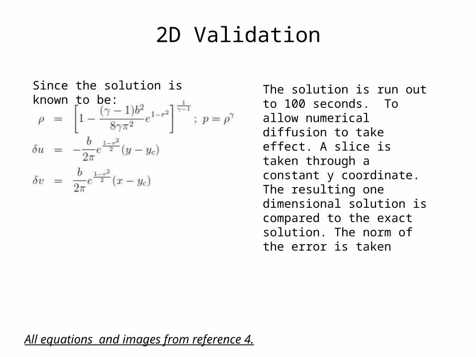
Since the solution is known to be: The solution is run out to 100 seconds. To allow numerical diffusion to take effect. A slice is taken through a constant y coordinate. The resulting one dimensional solution is compared to the exact solution. The norm of the error is taken

2D Validation

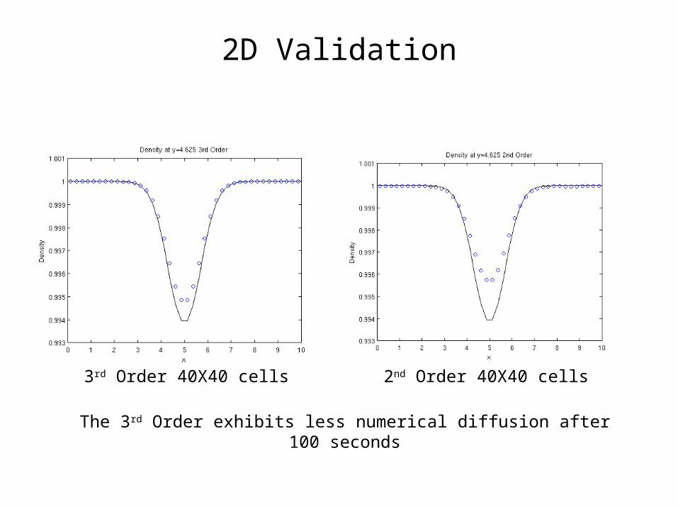
3rd Order 40X40 cells 2nd Order 40X40 cells

The 3rd Order exhibits less numerical diffusion after 100 seconds

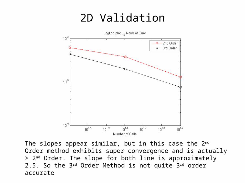
2D Validation

The slopes appear similar, but in this case the 2nd Order method exhibits super convergence and is actually > 2nd Order. The slope for both line is approximately 2.5. So the 3rd Order Method is not quite 3rd order accurate

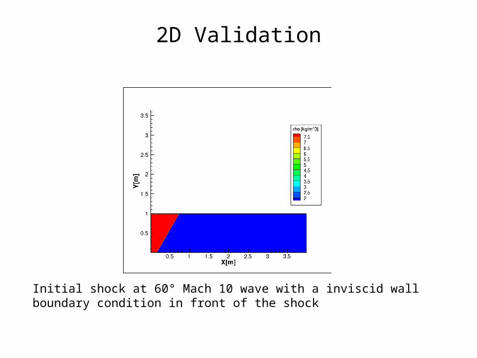
2D Validation

Initial shock at 60° Mach 10 wave with a inviscid wall boundary condition in front of the shock

Exact Solution Does Not Exist For The Double Mach Reflection Problem Visual Comparison Between Papers Is Required

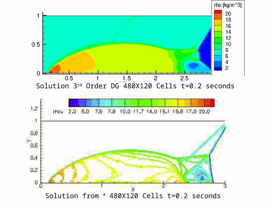
Solution 3rd Order DG 480X120 Cells t=0.2 seconds

Solution from 4 480X120 Cells t=0.2 seconds

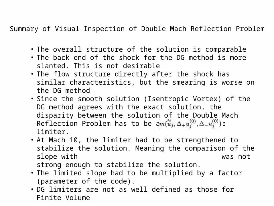
Summary of Visual Inspection of Double Mach Reflection Problem

• The overall structure of the solution is comparable • The back end of the shock for the DG method is more slanted. This is not

desirable• The flow structure directly after the shock has similar characteristics, but

the smearing is worse on the DG method• Since the smooth solution (Isentropic Vortex) of the DG method agrees

with the exact solution, the disparity between the solution of the Double Mach Reflection Problem has to be attributed to the limiter.

• At Mach 10, the limiter had to be strengthened to stabilize the solution. Meaning the comparison of the slope with was not strong enough to stabilize the solution.

• The limited slope had to be multiplied by a factor (parameter of the code).• DG limiters are not as well defined as those for Finite Volume

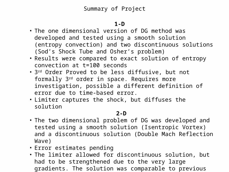
Summary of Project

1-D • The one dimensional version of DG method was developed and tested

using a smooth solution (entropy convection) and two discontinuous solutions (Sod’s Shock Tube and Osher’s problem)

• Results were compared to exact solution of entropy convection at t=100 seconds

• 3rd Order Proved to be less diffusive, but not formally 3rd order in space. Requires more investigation, possible a different definition of error due to time-based error.

• Limiter captures the shock, but diffuses the solution2-D

• The two dimensional problem of DG was developed and tested using a smooth solution (Isentropic Vortex) and a discontinuous solution (Double Mach Reflection Wave)

• Error estimates pending• The limiter allowed for discontinuous solution, but had to be

strengthened due to the very large gradients. The solution was comparable to previous works, but did smear the solution near the shock

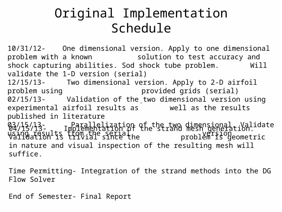
Original Implementation Schedule

10/31/12- One dimensional version. Apply to one dimensional problem with a known solution to test accuracy and shock capturing abilities. Sod shock tube problem. Will validate the 1-D version (serial)

12/15/13- Two dimensional version. Apply to 2-D airfoil problem using provided grids (serial)

02/15/13- Validation of the two dimensional version using experimental airfoil results as well as the results published in literature

03/15/13- Parallelization of the two dimensional. Validate using results from the serial version

04/15/13- Implementation of the strand mesh generation. Validation is trivial since the problem is geometric in nature and visual inspection of the resulting mesh will suffice.

Time Permitting- Integration of the strand methods into the DG Flow Solver

End of Semester- Final Report

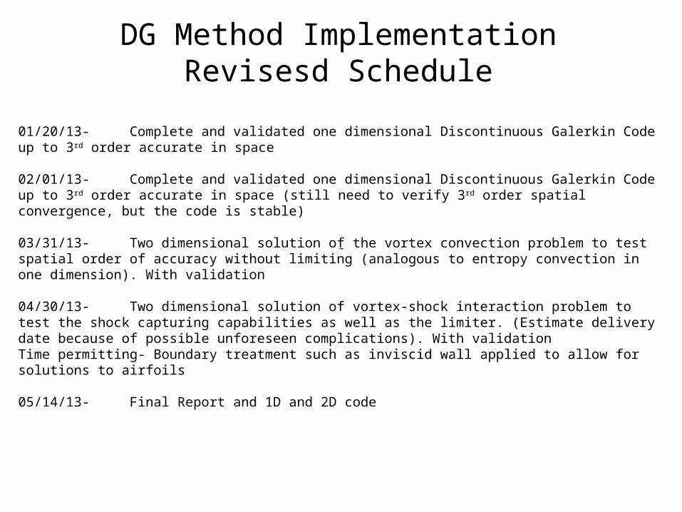
DG Method Implementation Revisesd Schedule

01/20/13- Complete and validated one dimensional Discontinuous Galerkin Code up to 3 rd order accurate in space

02/01/13- Complete and validated one dimensional Discontinuous Galerkin Code up to 3 rd order accurate in space (still need to verify 3rd order spatial convergence, but the code is stable)

03/31/13- Two dimensional solution of the vortex convection problem to test spatial order of accuracy without limiting (analogous to entropy convection in one dimension). With validation

04/30/13- Two dimensional solution of vortex-shock interaction problem to test the shock capturing capabilities as well as the limiter. (Estimate delivery date because of possible unforeseen complications). With validationTime permitting- Boundary treatment such as inviscid wall applied to allow for solutions to airfoils

05/14/13- Final Report and 1D and 2D code

Questions???

References:

1. Bernardo Cockburn, Chi-Wang Shu, The Runge-Kutta Discontinuous Galerkin Method for Cnservation Laws V, Multidimensional Systems, Journal of Computational Physics 141 199-224 (1997)

2. Bernardo Cockburn, Chi-Wang Shu, TVB Runge-Kutta Local Projection Discontinuous Galerkin Method for Conservation Laws II: General Frame Work Mathematics of Computation Volume 52 186 (1989)

3. Culbert B. Laney. Computational Gasdynamics. Cambridge University Press. 1998

4. D. Gosh, Compact-Reconstruction Weighted Essentially Non-Oscillatory Schemes for Hyperbolic Conservation Laws. Doctor of Philosophy Thesis, University of Maryland, College Park 2012.