Direct Stiffness MethodDSM FEM

8/7/2019 Direct Stiffness MethodDSM FEM

http://slidepdf.com/reader/full/direct-stiffness-methoddsm-fem 1/14

.

2The DirectStiffness Method I

2–1



Chapter 2: THE DIRECT STIFFNESS METHOD I 2–2

TABLE OF CONTENTS

Page

§2.1. Why A Plane Truss? 2–3§2.2. Truss Structures 2–3

§2.3. Idealization 2–4

§2.4. Members, Joints, Forces and Displacements 2–4

§2.5. The Master Stiffness Equations 2–6

§2.6. The DSM Steps 2–7

§2.7. Breakdown 2–7

§2.7.1. Disconnection . . . . . . . . . . . . . . . . . 2–7

§2.7.2. Localization . . . . . . . . . . . . . . . . . 2–8

§2.7.3. Computation of Member Stiffness Equations . . . . . . . 2–8

§2.8. Assembly: Globalization 2–9§2.8.1. Coordinate Transformations . . . . . . . . . . . . 2–9

§2.8.2. Transformation to Global System . . . . . . . . . . . 2–11

§2. Notes and Bibliography. . . . . . . . . . . . . . . . . . . . . . 2–12

§2. References . . . . . . . . . . . . . . . . . . . . . . 2–12

§2. Exercises . . . . . . . . . . . . . . . . . . . . . . 2–13

2–2



2–3 §2.2 TRUSS STRUCTURES

This Chapter begins the exposition of the Direct Stiffness Method (DSM) of structural analysis. The

DSM is by far the most common implementation of the Finite Element Method (FEM). In particular,

all major commercial FEM codes are based on the DSM.

The exposition is done by following the DSM steps applied to a simple plane truss structure. The

method has two major stages: breakdown, and assembly+solution. This Chapter covers primarily

the breakdown stage.

§2.1. Why A Plane Truss?

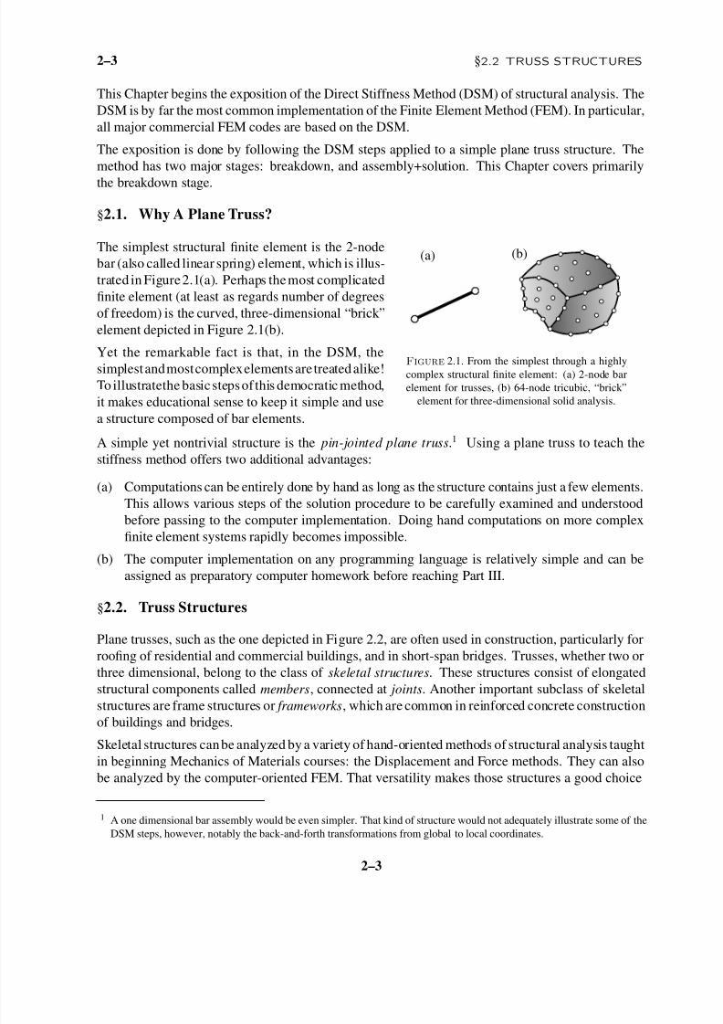
The simplest structural finite element is the 2-node

bar (also called linear spring) element, which is illus-

trated in Figure2.1(a). Perhaps themost complicated

finite element (at least as regards number of degrees

of freedom) is the curved, three-dimensional “brick ”

element depicted in Figure 2.1(b).

Yet the remarkable fact is that, in the DSM, thesimplestandmostcomplexelementsare treatedalike!

To illustratethe basicstepsof this democratic method,

it makes educational sense to keep it simple and use

a structure composed of bar elements.

(a) (b)

Figure 2.1. From the simplest through a highlycomplex structural finite element: (a) 2-node bar

element for trusses, (b) 64-node tricubic, “brick ”

element for three-dimensional solid analysis.

A simple yet nontrivial structure is the pin-jointed plane truss.1 Using a plane truss to teach the

stiffness method offers two additional advantages:

(a) Computations can be entirely done by hand as long as the structure contains just a few elements.

This allows various steps of the solution procedure to be carefully examined and understood

before passing to the computer implementation. Doing hand computations on more complex

finite element systems rapidly becomes impossible.(b) The computer implementation on any programming language is relatively simple and can be

assigned as preparatory computer homework before reaching Part III.

§2.2. Truss Structures

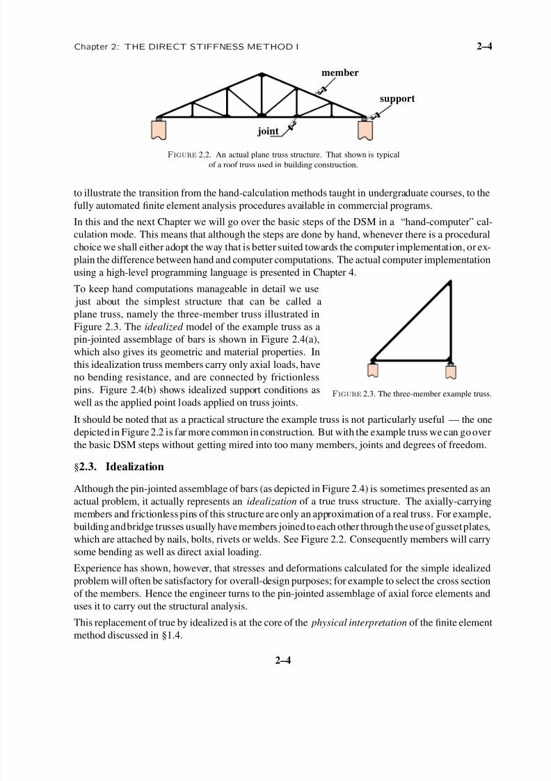
Plane trusses, such as the one depicted in Figure 2.2, are often used in construction, particularly for

roofing of residential and commercial buildings, and in short-span bridges. Trusses, whether two or

three dimensional, belong to the class of skeletal structures. These structures consist of elongated

structural components called members, connected at joints. Another important subclass of skeletal

structures are frame structures or frameworks, which are common in reinforced concrete construction

of buildings and bridges.

Skeletal structures canbe analyzed by a variety of hand-oriented methods of structural analysis taught

in beginning Mechanics of Materials courses: the Displacement and Force methods. They can also

be analyzed by the computer-oriented FEM. That versatility makes those structures a good choice

1 A one dimensional bar assembly would be even simpler. That kind of structure would not adequately illustrate some of the

DSM steps, however, notably the back-and-forth transformations from global to local coordinates.

2–3




joint

support

member

Figure 2.2. An actual plane truss structure. That shown is typical

of a roof truss used in building construction.

to illustrate the transition from the hand-calculation methods taught in undergraduate courses, to the

fully automated finite element analysis procedures available in commercial programs.

In this and the next Chapter we will go over the basic steps of the DSM in a “hand-computer” cal-

culation mode. This means that although the steps are done by hand, whenever there is a procedural

choice we shall either adopt the way that is better suited towards the computer implementation, or ex-

plain the difference between hand and computer computations. The actual computer implementation

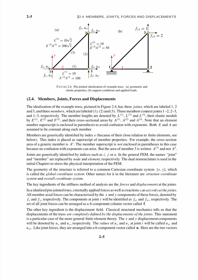
using a high-level programming language is presented in Chapter 4.To keep hand computations manageable in detail we use

just about the simplest structure that can be called a

plane truss, namely the three-member truss illustrated in

Figure 2.3. The idealized model of the example truss as a

pin-jointed assemblage of bars is shown in Figure 2.4(a),

which also gives its geometric and material properties. In

this idealization truss members carry only axial loads, have

no bending resistance, and are connected by frictionless

pins. Figure 2.4(b) shows idealized support conditions as

well as the applied point loads applied on truss joints.Figure 2.3. The three-member example truss.

It should be noted that as a practical structure the example truss is not particularly useful — the one

depicted in Figure 2.2 is far more common in construction. But with the example truss we can go over

the basic DSM steps without getting mired into too many members, joints and degrees of freedom.

§2.3. Idealization

Although the pin-jointed assemblage of bars (as depicted in Figure 2.4) is sometimes presented as an

actual problem, it actually represents an idealization of a true truss structure. The axially-carrying

members and frictionless pins of this structure are only an approximation of a real truss. For example,

buildingandbridge trusses usually havemembers joinedto each other through theuseof gussetplates,

which are attached by nails, bolts, rivets or welds. See Figure 2.2. Consequently members will carry

some bending as well as direct axial loading.

Experience has shown, however, that stresses and deformations calculated for the simple idealized

problem will often be satisfactory for overall-design purposes; for example to select the cross section

of the members. Hence the engineer turns to the pin-jointed assemblage of axial force elements and

uses it to carry out the structural analysis.

This replacement of true by idealized is at the core of the physical interpretation of the finite element

method discussed in §1.4.

2–4



2–5 §2.4 MEMBERS, JOINTS, FORCES AND DISPLACEMENTS

(a) (b)

E A = 100

E A = 50

E A

=200

√ 2

1 2

3

L = 10

L = 10 L = 10

√ 2

x

y

f , u y1 y1

f , u x1 x1 f , u x2 x2

f , u y2 y2

f , u x3 x3

f , u y3 y3

x

y

;

;

;

;

;

;

;

;

;

;

;

;

f x3 = 2

f y3 = 1

1 2

3

(3)

(3) (3)

(1)

(1) (1)

(2)

(2) (2)

(1)

(2)(3)

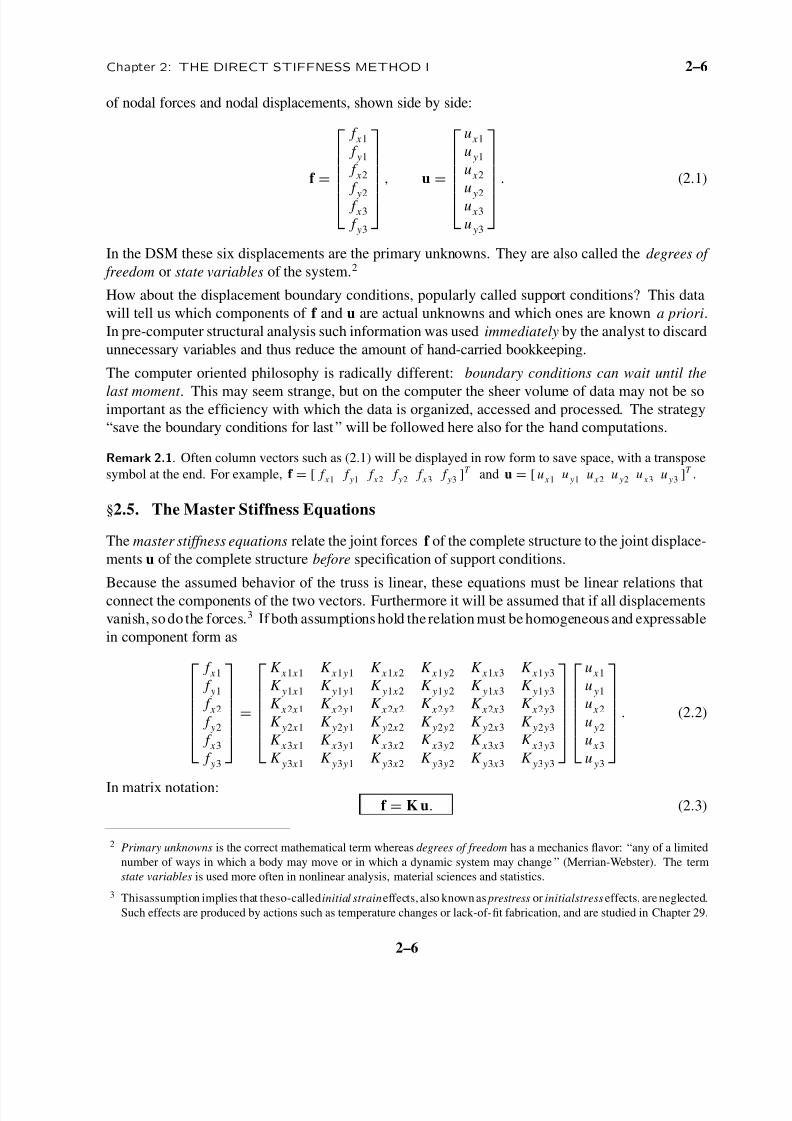
Figure 2.4. Pin-jointed idealization of example truss: (a) geometric and

elastic properties, (b) support conditions and applied loads.

§2.4. Members, Joints, Forces and Displacements

The idealization of the example truss, pictured in Figure 2.4, has three joints, which are labeled 1, 2

and3, and three members, which are labeled (1), (2) and (3). These members connect joints 1–2, 2–3,

and 1–3, respectively. The member lengths are denoted by L(1), L(2) and L(3), their elastic moduli

by E (1), E (2) and E (3), and their cross-sectional areas by A(1), A(2) and A(3). Note that an element

number superscript is enclosed in parenthesis to avoid confusion with exponents. Both E and A are

assumed to be constant along each member.

Members are generically identified by index e (because of their close relation to finite elements, see

below). This index is placed as superscript of member properties. For example, the cross-section

area of a generic member is Ae. The member superscript is not enclosed in parentheses in this case

because no confusion with exponents can arise. But the area of member 3 is written A(3) and not A3.

Joints are generically identified by indices such as i , j or n. In the general FEM, the names “ joint”

and “member” are replaced by node and element , respectively. The dual nomenclature is used in the

initial Chapters to stress the physical interpretation of the FEM.

The geometry of the structure is referred to a common Cartesian coordinate system { x, y}, which

is called the global coordinate system. Other names for it in the literature are structure coordinate

system and overall coordinate system.

The key ingredients of the stiffness method of analysis are the forces and displacements at the joints.

In a idealizedpin-jointed truss, externally applied forces as well as reactions can act only at the joints.

All member axial forces can be characterized by the x and y components of these forces, denoted by f x and f y , respectively. The components at joint i will be identified as f xi and f yi , respectively. The

set of all joint forces can be arranged as a 6-component column vector called f .

The other key ingredient is the displacement field. Classical structural mechanics tells us that the

displacements of the truss are completely defined by the displacements of the joints. This statement

is a particular case of the more general finite element theory. The x and y displacement components

will be denoted by u x and u y , respectively. The values of u x and u y at joint i will be called u xi and

u yi . Like joint forces, they are arranged into a 6-component vector called u. Here are the two vectors

2–5




of nodal forces and nodal displacements, shown side by side:

f

=

f x1

f y1

f x2

f y2

f x3

f y3

, u

=

u x1

u y1

u x2

u y2

u x3

u y3

. (2.1)

In the DSM these six displacements are the primary unknowns. They are also called the degrees of

freedom or state variables of the system.2

How about the displacement boundary conditions, popularly called support conditions? This data

will tell us which components of f and u are actual unknowns and which ones are known a priori.

In pre-computer structural analysis such information was used immediately by the analyst to discard

unnecessary variables and thus reduce the amount of hand-carried bookkeeping.

The computer oriented philosophy is radically different: boundary conditions can wait until the

last moment . This may seem strange, but on the computer the sheer volume of data may not be soimportant as the ef ficiency with which the data is organized, accessed and processed. The strategy

“save the boundary conditions for last” will be followed here also for the hand computations.

Remark 2.1. Often column vectors such as (2.1) will be displayed in row form to save space, with a transpose

symbol at the end. For example, f = [ f x1 f y1 f x2 f y2 f x3 f y3 ]T and u = [ u x1 u y1 u x2 u y2 u x3 u y3 ]T .

§2.5. The Master Stiffness Equations

The master stiffness equations relate the joint forces f of the complete structure to the joint displace-

ments u of the complete structure before specification of support conditions.

Because the assumed behavior of the truss is linear, these equations must be linear relations thatconnect the components of the two vectors. Furthermore it will be assumed that if all displacements

vanish, so do the forces.3 If both assumptions hold the relation must be homogeneous and expressable

in component form as

f x1

f y1

f x2

f y2

f x3

f y3

=

K x1 x1 K x1 y1 K x1 x2 K x1 y2 K x1 x3 K x1 y3

K y1 x1 K y1 y1 K y1 x2 K y1 y2 K y1 x3 K y1 y3





u x1

u y1

u x2

u y2

u x3

u y3

. (2.2)

In matrix notation:f = K u. (2.3)

2 Primary unknowns is the correct mathematical term whereas degrees of freedom has a mechanics flavor: “any of a limited

number of ways in which a body may move or in which a dynamic system may change ” (Merrian-Webster). The term

state variables is used more often in nonlinear analysis, material sciences and statistics.

3 Thisassumption implies that theso-called initial straineffects, also known as prestress or initialstress effects, are neglected.

Such effects are produced by actions such as temperature changes or lack-of-fit fabrication, and are studied in Chapter 29.

2–6



2–7 §2.7 BREAKDOWN

Here K is the master stiffness matrix, also called global stiffness matrix, assembled stiffness matrix,

or overall stiffness matrix. It is a 6 × 6 square matrix that happens to be symmetric, although this

attribute has not been emphasized in the written-out form (2.2). The entries of the stiffness matrix

are often called stiffness coef ficients and have a physical interpretation discussed below.

The qualifiers (“master”, “global”, “assembled” and “overall”) convey the impression that there is

another level of stiffness equations lurking underneath. And indeedthere is a member level or element level, into which we plunge in the Breakdown section.

Remark 2.2. Interpretation of Stiffness Coef ficients. The following interpretation of the entries of K is valuable

for visualization and checking. Choose a displacement vector u such that all components are zero except the

i th one, which is one. Then f is simply the i th column of K. For instance if in (2.3) we choose u x2 as unit

displacement,

u = [ 0 0 1 0 0 0 ]T , f = [ K x1 x2 K y1 x2 K x2 x2 K y2 x2 K x3 x2 K y3 x2 ]T . (2.4)

Thus K y1 x2, say, represents the y-force at joint 1 that would arise on prescribing a unit x-displacement at joint

2, while all other displacements vanish. In structural mechanics this property is called interpretation of stiffness

coef ficients as displacement in fl uence coef ficients. It extends unchanged to the general finite element method.

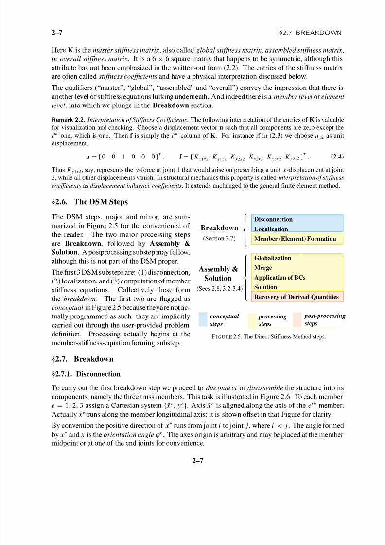
§2.6. The DSM Steps

The DSM steps, major and minor, are sum-

marized in Figure 2.5 for the convenience of

the reader. The two major processing steps

are Breakdown, followed by Assembly &

Solution. A postprocessing substepmayfollow,

although this is not part of the DSM proper.

The first3 DSMsubsteps are: (1)disconnection,

(2) localization, and(3) computation of member

stiffness equations. Collectively these form

the breakdown. The first two are flagged as

conceptual inFigure2.5 because theyare not ac-

tually programmed as such: they are implicitly

carried out through the user-provided problem

definition. Processing actually begins at the

member-stiffness-equation forming substep.

Disconnection

Localization

Member (Element) Formation

Globalization

Merge

Application of BCs

Solution

Recovery of Derived Quantities

Breakdown

Assembly &

Solution

(Section 2.7)

(Secs 2.8, 3.2-3.4)

post-processing

steps processing

steps

conceptual

steps

Figure 2.5. The Direct Stiffness Method steps.

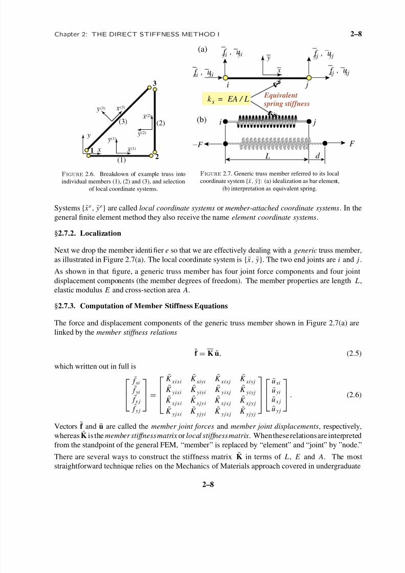
§2.7. Breakdown

§2.7.1. Disconnection

To carry out the first breakdown step we proceed to disconnect or disassemble the structure into its

components, namely the three truss members. This task is illustrated in Figure 2.6. To each member

e = 1, 2, 3 assign a Cartesian system { ¯ xe, ¯ ye}. Axis ¯ xe is aligned along the axis of the eth member.

Actually ¯ xe runs along the member longitudinal axis; it is shown offset in that Figure for clarity.

By convention the positive direction of ¯ xe runs from joint i to joint j , where i < j . The angle formed

by ¯ xe and x is the orientation angle ϕe. The axes origin is arbitrary and may be placed at the member

midpoint or at one of the end joints for convenience.

2–7




12

3

y

x

(3)

(1)

(2)

y_

(1)

x_

(1)

y_

(2)

x_

(2)

y_

(3) x_

(3)

Figure 2.6. Breakdown of example truss into

individual members (1), (2) and (3), and selection

of local coordinate systems.

i

i

j

j

d L

x

Equivalent

spring stiffnesss

−F F

f , u xi xi

_ _ f , u xj xj

_ _

f , u yj yj

_ _ f , u yi yi

_

_ y_

_

k = EA / L

(a)

(b)

Figure 2.7. Generic truss member referred to its local

coordinate system { ¯ x, ¯ y}: (a) idealization as bar element,

(b) interpretation as equivalent spring.

Systems { ¯ xe, ¯ ye} are called local coordinate systems or member-attached coordinate systems. In the

general finite element method they also receive the name element coordinate systems.

§2.7.2. Localization

Next we drop the member identifier e so that we are effectively dealing with a generic truss member,

as illustrated in Figure 2.7(a). The local coordinate system is { ¯ x, ¯ y}. The two end joints are i and j .

As shown in that figure, a generic truss member has four joint force components and four joint

displacement components (the member degrees of freedom). The member properties are length L,

elastic modulus E and cross-section area A.

§2.7.3. Computation of Member Stiffness Equations

The force and displacement components of the generic truss member shown in Figure 2.7(a) are

linked by the member stiffness relations

f = K u, (2.5)

which written out in full is

¯ f xi

¯ f yi

¯ f x j¯ f y j

=

K xixi K xiyi K xixj K xiyj

K yixi K yiyi K yixj K yiyj

K xjxi K xjyi K xjxj K xjyj

K yjxi K yjyi K yjxj K yjyj

u xi

u yi

u x ju y j

. (2.6)

Vectors f and u are called the member joint forces and member joint displacements, respectively,

whereas K is the member stiffnessmatrix or local stiffnessmatrix. Whentheserelationsare interpreted

from the standpoint of the general FEM, “member” is replaced by “element” and “ joint” by ”node.”

There are several ways to construct the stiffness matrix K in terms of L, E and A. The most

straightforward technique relies on the Mechanics of Materials approach covered in undergraduate

2–8



2–9 §2.8 ASSEMBLY: GLOBALIZATION

courses. Think of the truss member in Figure 2.7(a) as a linear spring of equivalent stiffness k s ,

an interpretation illustrated in Figure 2.7(b). If the member properties are uniform along its length,

Mechanics of Materials bar theory tells us that4

k s

= E A

L

, (2.7)

Consequently the force-displacement equation is

F = k sd = E A

Ld , (2.8)

where F is the internal axial force and d the relative axial displacement, which physically is the bar

elongation. The axial force and elongation can be immediately expressed in terms of the joint forces

and displacements as

F = ¯ f x j = − ¯ f xi , d = u x j − u xi , (2.9)

which express force equilibrium5

and kinematic compatibility, respectively. Combining (2.8) and(2.9) we obtain the matrix relation6

f =

¯ f xi

¯ f yi

¯ f x j

¯ f y j

= E A

L

1 0 −1 0

0 0 0 0

−1 0 1 0

0 0 0 0

u xi

u yi

u x j

u y j

= K u, (2.10)

Hence

K = E A

L

1 0 −1 0

0 0 0 0

−1 0 1 0

0 0 0 0

. (2.11)

This is the truss stiffness matrix in local coordinates.

Two other methods for obtaining the local force-displacement relation (2.8) are covered in Exercises

2.6 and 2.7.

§2.8. Assembly: Globalization

The first substep in the assembly & solution major step, as shown in Figure 2.5, is globalization.

This operation is done member by member. It refers the member stiffness equations to the global

system

{ x, y

}so it can be merged into the master stiffness. Before entering into details we must

establish relations that connect joint displacements and forces in the global and local coordinate

systems. These are given in terms of transformation matrices.

4 See for example, Chapter 2 of [19].

5 Equations F = ¯ f x j = − ¯ f xi follow by considering the free body diagram (FBD) of each joint. For example, take joint i as

a FBD. Equilibrium along x requires −F − ¯ f xi = 0 whence F = − ¯ f xi . Doing the same on joint j yields F = ¯ f x j .

6 The matrix derivation of (2.10) is the subject of Exercise 2.3.

2–9




x

y

(a) Displacement

transformation

(b) Force

transformation

i

j

ϕ

f xi

f yi

f xj

f yj

f yi

_

f xi

_

f xj

_ f yj

_

i

x y j

ϕ

u xi

u yi

u xj

u yj

u yi _

_ _

u xi

_

u xj

_u yj

_

Figure 2.8. The transformation of node displacement and force

components from the local system { ¯ x, ¯ y} to the global system { x, y}.

§2.8.1. Coordinate Transformations

The necessary transformations are easily obtained by inspection of Figure 2.8. For the displacements

u xi = u xi c + u yi s, u yi = −u xi s + u yi c,

u x j = u x j c + u y j s, u y j = −u x j s + u y j c,. (2.12)

where c = cos ϕ, s = sin ϕ and ϕ is the angle formedby ¯ x and x , measuredpositive counterclockwise

from x . The matrix form of this relation is

u xi

u yi

u x j

u y j

=

c s 0 0

−s c 0 0

0 0 c s

0 0 −s c

u xi

u yi

u x j

u y j

. (2.13)

The 4 × 4 matrix that appears above is called a displacement transformation matrix and is denoted7

by T. The node forces transform as f xi = ¯ f xi c − ¯ f yi s, etc., which in matrix form become

f xi

f yi

f x j

f y j

=

c −s 0 0

s c 0 0

0 0 c −s

0 0 s c

¯ f xi¯ f yi

¯ f x j

¯ f y j

. (2.14)

The 4

×4 matrix that appears above is called a force transformation matrix. A comparison of

(2.13) and (2.14) reveals that the force transformation matrix is the transpose TT of the displacementtransformation matrix T. This relation is not accidental and can be proved to hold generally.8

7 This matrix will be called Td when its association with displacements is to be emphasized, as in Exercise 2.5.

8 A simple proof that relies on the invariance of external work is given in Exercise 2.5. However this invariance was only

checked by explicit computation for a truss member in Exercise 2.4. The general proof relies on the Principle of Virtual

Work, which is discussed later.

2–10



2–11 §2.8 ASSEMBLY: GLOBALIZATION

Remark 2.3. Note that in (2.13) the local system (barred) quantities appear on the left-hand side, whereas in

(2.14) they show up on the right-hand side. The expressions (2.13) and and (2.14) are discrete counterparts

of what are called covariant and contravariant transformations, respectively, in continuum mechanics. The

continuum counterpart of the transposition relation is called adjointness. Colectively these relations, whether

discrete or continuous, pertain to the subject of duality.

Remark 2.4. For this particular structural element T is square and orthogonal, that is, TT = T−1. But thisproperty does not extend to more general elements. Furthermore in the general case T is not even a square

matrix, and does not possess an ordinary inverse. However the congruent transformation relations (2.15)–(2.17)

do hold generally.

§2.8.2. Transformation to Global System

From now on we reintroduce the member (element) index, e. The member stiffness equations in

global coordinates will be written

f e = Keue. (2.15)

The compact form of (2.13) and (2.14) for the eth member is

ue = Teue, f e = (Te)T f e

. (2.16)

Inserting thesematrix expressions into f e = K

eue andcomparingwith (2.15) we find that the member

stiffness in theglobalsystem { x, y} canbe computed from themember stiffness Ke

in the local system

{ ¯ x, ¯ y} through the congruent transformation9

Ke = (Te)T KeTe. (2.17)

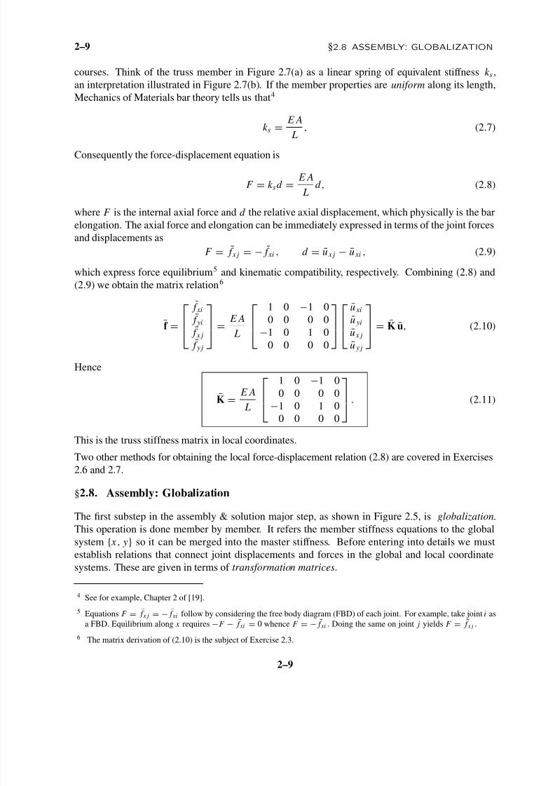
Carrying out the matrix multiplications in closed form (Exercise 2.8) we get

Ke = E e Ae

Le

c2 sc −c2 −sc

sc s2 −sc −s2

−c2 −sc c2 sc

−sc −s2 sc s2

, (2.18)

in which c = cos ϕe, s = sin ϕe, with e superscripts of c and s suppressed to reduce clutter. If the

angle is zero we recover (2.10), as may be expected. Ke is called a member stiffness matrix in global

coordinates. The proof of (2.17) and verification of (2.18) is left as Exercise 2.8.

The globalized member stiffness matrices for the example truss can now be easily obtained by

inserting appropriate values into (2.18). For member (1), with end joints 1–2, angle ϕ(1) = 0◦ and

the member properties given in Figure 2.4(a) we get

f (1)

x1

f (1)

y1

f (1)

x2

f (1)

y2

= 10

1 0 −1 0

0 0 0 0

−1 0 1 0

0 0 0 0

u(1)

x1

u(1)

y1

u(1)

x2

u(1)

y2

. (2.19)

9 Also known as congruential transformation and congruence transformation in linear algebra books.

2–11




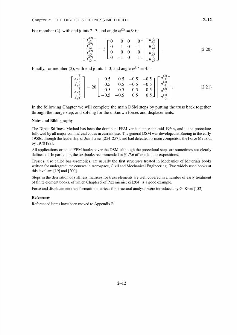
For member (2), with end joints 2–3, and angle ϕ(2) = 90◦:

f (2)

x2

f (2)

y2

f (2)

x3

f (2) y3

= 5

0 0 0 0

0 1 0 −1

0 0 0 0

0 −1 0 1

u(2)

x2

u(2)

y2

u(2)

x3

u(2) y3

. (2.20)

Finally, for member (3), with end joints 1–3, and angle ϕ(3) = 45◦:

f (3)

x1

f (3)

y1

f (3)

x3

f (3)

y3

= 20

0.5 0.5 −0.5 −0.5

0.5 0.5 −0.5 −0.5

−0.5 −0.5 0.5 0.5

−0.5 −0.5 0.5 0.5

u(3)

x1

u(3)

y1

u(3)

x3

u(3)

y3

. (2.21)

In the following Chapter we will complete the main DSM steps by putting the truss back together

through the merge step, and solving for the unknown forces and displacements.

Notes and Bibliography

The Direct Stiffness Method has been the dominant FEM version since the mid-1960s, and is the procedure

followed by all major commercial codes in current use. The general DSM was developed at Boeing in the early

1950s, through the leadership of Jon Turner [254–257], and had defeated its main competitor, the Force Method,

by 1970 [88].

All applications-oriented FEM books cover the DSM, although the procedural steps are sometimes not clearly

delineated. In particular, the textbooks recommended in §1.7.6 offer adequate expositions.

Trusses, also called bar assemblies, are usually the first structures treated in Mechanics of Materials books

written for undergraduate courses in Aerospace, Civil and Mechanical Engineering. Two widely used books at

this level are [19] and [200].

Steps in the derivation of stiffness matrices for truss elements are well covered in a number of early treatmentof finite element books, of which Chapter 5 of Przemieniecki [204] is a good example.

Force and displacement transformation matrices for structural analysis were introduced by G. Kron [152].

References

Referenced items have been moved to Appendix R.

2–12



2–13 Exercises

Homework Exercises for Chapter 2

The Direct Stiffness Method I

EXERCISE 2.1 [D:10] Explain why arbitrarily oriented mechanical loads on an idealized pin-jointed truss

structure must be applied at the joints. [Hint: idealized truss members have no bending resistance.] How about

actual trusses: can they take loads applied between joints?

EXERCISE 2.2 [A:15] Show that the sum of the entries of each row of the master stiffness matrix K of any

plane truss, before application of any support conditions, must be zero. [Hint: apply translational rigid body

motions at nodes.] Does the property hold also for the columns of that matrix?

EXERCISE 2.3 [A:15] Using matrix algebra derive (2.10) from (2.8) and (2.9). Note: Place all equations in

matrix form first and eliminate d and F by matrix multiplication. Deriving the final form with scalar algebra

and rewriting it in matrix form gets no credit.

EXERCISE 2.4 [A:15] By direct multiplication verify that for the truss member of Figure 2.7(a), f T

u = F d .

Intepret this result physically. (Hint: what is a force times displacement in the direction of the force?)

EXERCISE 2.5 [A:20] The transformation equations between the 1-DOF spring and the 4-DOF generic trussmember may be written in compact matrix form as

d = Td u, f = F T f , (E2.1)

where Td is 1 × 4 and T f is 4 × 1. Starting from the identity f T

u = F d proven in the previous exercise, and

using compact matrix notation, show that T f = TT d . Or in words: the displacement transformation matrix and

the force transformation matrix are the transpose of each other . (This can be extended to general systems)

EXERCISE 2.6 [A:20] Derive the equivalent springformula F = ( E A/ L) d of (2.8) by the Theory of Elasticity

relations e = d u( ¯ x)/d ¯ x (strain-displacement equation), σ = Ee (Hooke’s law) and F = Aσ (axial force

definition). Here e is the axial strain (independent of ¯ x) and σ the axial stress (also independent of ¯ x). Finally,

¯u(

¯ x) denotes the axial displacementof thecross section at a distance

¯ x from node i , which is linearly interpolated

as

u( ¯ x) = u xi

1 − ¯ x

L

+ u x j

¯ x L

(E2.2)

Justify that (E2.2) is correct since the bar differential equilibrium equation: d [ A(d σ/d ¯ x)]/d ¯ x = 0, is verified

for all ¯ x if A is constant along the bar.

EXERCISE 2.7 [A:20] Derive the equivalent spring formula F = ( E A/ L) d of (2.8) by the principle of

Minimum Potential Energy (MPE). In Mechanics of Materials it is shown that the total potential energy of the

axially loaded bar is

= 1

2

L

0

A σ e d ¯ x − Fd , (E2.3)

where symbols have the same meaning as the previous Exercise. Use the displacement interpolation (E2.2),

the strain-displacement equation e = d u/d ¯ x and Hooke’s law σ = Ee to express as a function (d ) of the

relative displacement d only. Then apply MPE by requiring that ∂/∂d = 0.

EXERCISE 2.8 [A:20] Derive (2.17) from Keue = f

e, (2.15) and (2.17). ( Hint : premultiply both sides of

Keue = f

eby an appropriate matrix). Then check by hand that using that formula you get (2.18). Falk ’s scheme

is recommended for the multiplications.10

10 This scheme is useful to do matrix multiplication by hand. It is explained in §B.3.2 of Appendix B.

2–13




EXERCISE 2.9 [D:5] Why are disconnection and localization labeled as “conceptual steps” in Figure 2.5?

EXERCISE 2.10 [C:20] (Requires thinking) Notice that the expression (2.18) of the globalized bar stiffness

matrix may be factored as

Ke = E

e

A

e

Le

c2 sc −c2 −sc

sc s2

−sc −s2

−c2 −sc c2 sc

−sc −s2 sc s2

= −c

−sc

s

E

e

A

e

Le[ −c −s c s ] (E2.4)

Interpret this relation physically as a chain of global-to-local-to-global matrix operations: global displacements

→ axial strain, axial strain → axial force, and axial force → global node forces.

2–14

Documents

Direct Stiffness MethodDSM FEM