Contemporary Mathematics

Dirac operators, Boundary Value Problems, and the

b-Calculus

Paul Loya

Abstract. It is well-known that the index of a Dirac operator with augmented

Atiyah-Patodi-Singer (= APS) boundary conditions on a compact manifold

with boundary can be identified with the L2 index of a corresponding operator

on a manifold with cylindrical ends. The augmented APS condition is a specific

example of an “ideal boundary condition,” which is a boundary condition thatdiffers from the APS condition by a projection on the kernel of the boundaryDirac operator. Following Melrose and Piazza [42] we show that the indexand eta invariants of a Dirac operator on a compact manifold with boundarywith any ideal boundary condition can be identified with parallel invariantsof a perturbation of the corresponding Dirac operator on the manifold withcylindrical ends with L2 domain by a b-smoothing operator constructed from

the ideal boundary condition. In this sense, the “b-category” of objects is ableto give a complete description of index and eta invariants for all ideal boundary

conditions, and not just the augmented APS condition.

1. Introduction

Two of the most basic and most studied invariants describing to different de-grees the spectral asymmetry of Dirac operators are the index and eta invariants.The index describes the asymmetry of the kernel and the eta invariant describes theasymmetry of the entire spectrum of Dirac operators. The purpose of this article isto relate these invariants on manifolds with boundary to corresponding invariantson manifolds with cylindrical ends.

1.1. Ideal boundary conditions and the index theorem. The seminalpapers [4, 5] by Atiyah, Patodi, and Singer created immense investigations intoindex theory on manifolds with boundary and singularities; to name only a fewextensions of their work, see for instance, Cheeger [14], Atiyah, Donnelly, andSinger [3], Muller [43], Stern [57], Bruning [11], Bismut and Cheeger [7, 8], Grubband Seeley [22] and many others; for survey articles treating various aspects ofindex theory, see Muller [46], Piazza [49], Seeley [55], or Loya [32]. In this paper

2000 Mathematics Subject Classification. Primary 58J28; Secondary 58J35, 58J20, 58J32.Key words and phrases. Atiyah-Patodi-Singer index theorem; Eta invariants; Boundary value

problems; Dirac operators; b-calculus.Supported in part by a Ford Foundation Fellowship.

c©2004 American Mathematical Society

1

2 PAUL LOYA

we shall focus our attention on Melrose’s [39, 40] b-calculus reinterpretation of theAtiyah, Patodi, and Singer (henceforth APS) index theorem, especially in regardsto the so-called “ideal boundary conditions”, which we now review.

We first set the stage by stating our assumptions and then we recall the aug-mented APS boundary condition. Let D : C∞(M,E) −→ C∞(M,F ) be an admis-sible (also called compatible) Dirac operator associated to a Z2-graded HermitianClifford module E ⊕ F →M over a compact, even-dimensional, Riemannian man-ifold with boundary. We assume that all the geometric structures are of producttype on a collar [0, 1)x×Y of the boundary Y of M , where x is a boundary definingfunction which is everywhere positive on the interior of M . Therefore, on this collarwe assume that E ∼= E|x=0, F ∼= F |x=0, the metric g on M takes the form

g = dx2 + h

with h a metric on Y , and finally,

(1.1) D = Γ(∂x +DY ),

where Γ : E|x=0 −→ F |x=0 is a unitary isomorphism (Clifford multiplication bydx) and where DY is a Dirac operator on Y . Since DY is a self-adjoint elliptic firstorder differential operator on a compact manifold without boundary, it has discretespectrum consisting of real numbers extending above and below zero to ±∞. LetΠ+ denote the orthogonal projection of L2(Y,EY ), where EY := E|x=0, onto theeigenspaces of DY corresponding to the positive eigenvalues.

Let V = kerDY and let Π0 denote the orthogonal projection of L2(Y,EY )onto V . Then there is a distinguished subspace ΛC of V (see Melrose [40], Muller[45, 44]) defined by

(1.2) ΛC :=Π0u|x=0 ; u ∈ H1(M,E), Du = 0, Π+u|x=0 = 0

.

If ΠC is the orthogonal projection onto ΛC , then C := 2ΠC − Id, acting on V ,is a unitary map on V with eigenvalues ±1 and with +1 eigenspace exactly ΛC .The unitary map C is called the scattering matrix and ΛC is called the scatteringLagrangian.1 This subspace is also known as the subspace corresponding to the“limiting values of extended L2 solutions of Du = 0” for the following reason. Let

M be the manifold formed by taking the infinite cylinder (−∞, 0]x × Y and gluingit onto the end of the collar [0, 1)x × Y of M :

M = (−∞, 0]x × Y t∂M M.

Since all the geometric structures and the Dirac operator are of product type on the

collar of M , they all have natural extensions to the manifold M . We denote these

extended structures on M using the same notations used for the original objects on

M ; however, since the extended Dirac operator on M acts on a different domain

than the Dirac operator on M , namely sections on M rather than on M , we denote

the extension of the Dirac operator by D. Then [40], [45]

(1.3) ΛC =

limx→−∞

u(x, y) ; u ∈ C∞(M,E) is bounded and Du = 0.

The manifold M will play very important roles as our story unfolds.

1This is really “half” of the true Lagrangian, which is ΛC ⊕ΓΛC ⊂ E ⊕F for the symplectic

structure given by the L2 inner product and the Clifford action Γ ⊕ (−Γ∗) : E ⊕ F −→ F ⊕ E.

BOUNDARY VALUE PROBLEMS AND THE B-CALCULUS 3

We now define the augmented APS boundary condition. The Dirac operatorD with domain

(1.4) Dom(DAPS) := u ∈ H1(M,E) ; (Π+ + ΠC)u|x=0 = 0defines the Dirac operator DAPS with the augmented APS boundary condition. TheAPS index theorem can then be written as

indDAPS =

∫

M

AS − 1

2η(DY ),

where AS is the Atiyah-Singer index density manufactured from the Clifford mod-ules and connection and where η(DY ) is the eta invariant of DY , to be discussedmore fully in Section 1.2.

Although C is in some sense canonical, it is possible, of course, to chooseother projections onto subspaces in V in (1.4) to define Dirac operators with otherdomains. Let T be a self-adjoint isomorphism on V with T 2 = Id. Then T has ±1eigenvalues. We define DT as the Dirac operator D with domain

(1.5) Dom(DT ) := u ∈ H1(M,E) ; ΠT+u|x=0 = 0,

where ΠT+ := Π+ + Π⊥

T with Π⊥T the orthogonal projection onto the −1 eigenspace

of T . Such a boundary condition is called an ideal boundary condition. Thus, DAPS

is really just D−C with C the scattering matrix.Before stating the first result in this paper we make a couple remarks about

some natural objects on M . First, we remark that there is a natural scale of L2

based Sobolev spaces on M , where square integrability means with respect to the

(extended) measure dg on M . In particular, the natural domain of D is H1(M,E),

which consists of those sections u on M such that Du is L2. Second, we remark

that various classes of pseudodifferential operators on M that preserve these Sobolevspaces have been developed by many different authors, to name a few, Egorov andSchulze [17], Melrose [40], Melrose and Mendoza [41], Plamenevskij [50], Rempeland Schulze [52], and Schulze [54]. These operators are more or less the same (cf.Lauter and Seiler [26]), but the operators we choose for the purposes of this paperare the (small calculus of) b-pseudodifferential operators of Melrose, to be explainedin Section 2.2. Of these operators, the b-smoothing operators (b-pseudodifferentialoperators of order −∞) will serve as a natural class of “perturbations” in the sequel.

With this background, we are ready to state the first theorem in this paper.

Theorem 1.1. Let D and D be as above and let T be a self-adjoint isomorphism

on V with T 2 = Id. Then there exists a b-smoothing operator T such that the L2

based operator D − T on the complete manifold M and the operator DT on thecompact manifold M have the same index theoretic properties:

(a) ker(D − T ) ∼= kerDT and ker(D − T )∗ ∼= ker(DT )∗.(b) The operators

D − T : H1(M,E) −→ L2(M, F ),

DT : Dom(DT ) −→ L2(M,F )

are Fredholm with (by (a)) equal indices.(c) The following index formula holds:

ind(D − T ) = indDT =

∫

M

AS − 1

2[η(DY ) − signT ].

4 PAUL LOYA

The equality in (a) was proved in joint work with Melrose [33]. In [42], Melroseand Piazza prove a families index theorem, which in the simplest case when the basemanifold is a point, consists of statements (b) and (c) but with T a very generalfinite rank operator (connected with the notion of a spectral section). Therefore,the equality of indices and the index formula in Properties (b) and (c) are specialcases of Melrose and Piazza’s theorem. In Theorem 3.4, we shall extend the index

formula (c) for ind(D − T ) to a slightly more general class of perturbations.

1.2. Ideal boundary conditions and the eta invariant. The eta invariantfor self-adjoint Dirac operators on odd -dimensional manifolds shares many proper-ties with the index (cf. Singer [56]) and has also become an area of much interestsince the publication of the seminal work of Atiyah, Patodi, and Singer [5]. Re-cently, many authors have focused on understanding the decomposition of the etainvariant under gluing of manifolds. Such “gluing problems” have been investigatedby, for instance, Dai and Freed [15], Muller [45], Wojciechowski [59, 60, 61], Bunke[13], Lesch and Wojciechowski [27], Mazzeo and Melrose [36], Hassell, Mazzeo, andMelrose [23], Bruning and Lesch [12], Kirk and Lesch [25], and Loya and Park [34].For surveys on such “cut and paste” formulas of the eta invariant see Mazzeo andPiazza [37] or Bleecker and Booß-Bavnbek [9]. One aspect of this gluing prob-lem involves the eta invariant on a manifold with boundary and its dependence onboundary conditions. Lagrangian subspaces and ideal boundary conditions comeinto the picture in order to get a self-adjoint Dirac operator.

Let D be a Dirac operator as considered in Section 1.1, however we now assumethat E = F and M is odd-dimensional. Of course, we still assume product struc-tures near the boundary as in (1.1), but now Γ is a unitary isomorphism on EYonly, since E = F . Moreover, Clifford and self-adjointness considerations imposethe following relations:

(1.6) Γ2 = −Id, Γ∗ = −Γ, ΓDY = −DY Γ.

As before, we set V := kerDY . Then the last equality in (1.6) implies that Γacts on V . The set of unitary isomorphisms T on V such that ΓT = −T Γ andT 2 = Id is denoted by L(V ). Such isomorphisms can be constructed as follows.First, observe that V = V + ⊕ V −, where V ± are the ±i eigenspaces of Γ. Notethat dimV + = dimV − by the cobordism invariance of the index, see Theorem 21.5of Booß-Bavnbek and Wojciechowski [10]. Then given any unitary isomorphismT+ : V + −→ V − and setting T− := (T+)−1, the map T := T+ + T− is inL(V ). Conversely, every element of L(V ) arises in this way. Given T ∈ L(V ),we denote the +1 eigenspace of T by ΛT . Note that ΓΛT is the −1 eigenspace ofT and that V = ΛT ⊕ ΓΛT is an orthogonal decomposition. One can check thatΩ(v, w) := Re(Γv, w)Y , where v, w ∈ V and where ( , )Y is the L2 inner producton Y , is a symplectic form on V , and that the subspaces of V that are Lagrangianwith respect to Ω are exactly those of the form ΛT for some T ∈ L(V ). Moreover,the scattering matrix C is an element of L(V ) with associated Lagrangian ΛC [45].

We now recall the definition of the eta invariant in the context of ideal boundaryconditions as presented in Appendix 1 of Douglas and Wojciechowski [16]. GivenT ∈ L(V ), recall that DT is the Dirac operator D with domain given in (1.5).Because T ∈ L(V ) and therefore ΛT is Lagrangian, it turns out that the operatorDT is self-adjoint and has real discrete spectrum. If λj are the eigenvalues of

BOUNDARY VALUE PROBLEMS AND THE B-CALCULUS 5

DT , then the eta function of DT ,

(1.7) η(z,DT ) :=∑

λj 6=0

signλj|λj |z

,

extends from Re z >> 0 to be a meromorphic function of z ∈ C that is regular atz = 0. The eta invariant, η(DT ), is defined as the number η(0,DT ). Thus, formallyspeaking, “η(DT ) =

∑λj 6=0 signλj” and hence, η(DT ) is a measure of the spectral

asymmetry of DT .As the scattering Lagrangian is canonically associated to the Dirac operator,

one can argue that the eta invariant with the augmented APS condition, η(D−C),provides an “origin” to which to compare eta invariants defined using other La-grangian subspaces. To support this statement, in [45] Muller proves that η(D−C)

is equal to the b-eta invariant bη(D) of the Dirac operator D on the corresponding

cylindrical end manifold M . The b-eta invariant of D is not defined via a formula

of the sort (1.7) because D has continuous and not discrete spectrum (as M is not

compact), but nevertheless is the natural generalization of the eta invariant to M ,see Section 4. Before presenting our second theorem, we need the following functionintroduced by Lesch and Wojciechowski in [27]: For T, S ∈ L(V ), we define

(1.8) m(ΛT ,ΛS) := − 1

iπ

∑

eiθ∈spec(−T−S+)θ∈(−π,π)

iθ.

Here, T− and S+ are the restrictions of T and S to the −i and +i eigenspaces ofΓ respectively. The second result of this note is the following.

Theorem 1.2. Let D and D be as above and let T ∈ L(V ). Then there exists

a b-smoothing operator T such that DT and the perturbed Dirac operator D − Thave the same eta invariant theoretic properties:

(a) ker(D − T ) ∼= ker(DT ).

(b) bη(D − T ) = η(DT ).(c) The following surgery formula holds:

bη(D − T ) = η(DT ) = η(D−C) +m(ΛT ,ΛC),

where C is the scattering matrix.

The equalitybη(D − T ) = η(D−C) +m(ΛT ,ΛC)

was proved in joint work with Melrose [33].As a corollary of Theorem 1.2, we obtain a formula for the dependence of the

eta invariant on different Lagrangian subspaces. To this end, let τ denote the tripleMaslov index, defined on a triple (ΛA,ΛB ,ΛC) of Lagrangian subspaces of V by

τ(ΛA,ΛB ,ΛC) := m(ΛA,ΛB) +m(ΛB ,ΛC) +m(ΛC ,ΛA).

Although the function m is real-valued, the triple index is integer-valued, see Bunke[13] and Lion and Vergne [29]. Theorem 1.2, the definition of τ , and the fact thatm is antisymmetric, imply the following corollary.

6 PAUL LOYA

Corollary 1.3. For any T, S ∈ L(V ), we have

η(DT ) − η(DS) = m(ΛT ,ΛS) + τ(ΛT ,ΛC ,ΛS),

where C is the scattering matrix.

1.3. Final remarks and outline of paper. The proofs of Theorem 1.1 and1.2 use the so-called heat kernel method which relies on taking traces of suitableheat operators, cf. Mckean and Singer [38], Patodi [48], Atiyah, Bott, and Patodi

[2], and Gilkey [19]. However, since M is not compact, it turns out that the

relevant heat operators are not trace class on M . To overcome this obstacle, weutilize a regularized trace called the b-trace2 developed by Melrose [40]. In manyrespects, the b-trace is the “hero” of this paper: We use it to make non-trace classheat operators “(b-) trace class;” give a direct derivation of the APS index formulawith the eta invariant emerging as a direct computation from the b-trace’s keyfeature, the trace-defect formula; we use it to define the b-eta invariant (withoutrequiring the Dirac operators to have discrete spectrum), and finally, we use it andthe trace-defect formula to prove the variation formula for the eta invariant via adirect computation.

The outline of this paper is as follows. We begin this paper in Section 2 byproving a simplified version of Theorem 1.1 in the case that the boundary Diracoperator is invertible. We also delve into a detailed study of b-pseudodifferentialoperators and we introduce the b-trace and derive its key feature: the trace-defect

formula. In Section 3, we define the b-smoothing perturbation T in Theorem 1.1 andwe prove this theorem via the general index theorem 3.4. The proof of Theorem1.2 is based on Vishik’s technique of rotating boundary conditions, see Section1 of [58], originally developed to prove gluing formulas for torsion invariants onmanifolds with boundary. In Section 4, we review this technique as refined byBruning and Lesch [12] for the study of eta invariants to prove Theorem 1.2.

In conclusion, I wish to thank Richard Melrose for sharing his insights intomany of these problems, Paolo Piazza for looking over parts of the manuscript, andKrzysztof Wojciechowski for his support and encouragement in proving Theorem1.2. I also thank the referee for thoughtful comments, finding many mistakes, andfor very helpful suggestions all of which led to many improvements. Finally, Ithank the organizers of the conference, Bernhelm Booß-Bavnbek, Gerd Grubb, andKrzysztof Wojciechowski, for allowing me to participate.

2. Transformation to b-objects I

In this section we prove a simplified version of Theorem 1.1 in the case thatthe boundary Dirac operator is invertible, which is a special case of Atiyah, Patodi,and Singer’s classic result [5]. We begin by reviewing the necessary ingredientsand then we move into a detailed study of b-pseudodifferential operators. Next, weintroduce the hero of this paper, the b-trace and its main feature: the trace-defectformula. Finally, we prove the index formula for the case that the boundary Diracoperator is invertible. Here we see our first instance of the trace-defect formula inaction in the direct manner in which the eta invariant appears in APS formula.

2The b-trace is almost the same as the relative trace found in Muller [47].

BOUNDARY VALUE PROBLEMS AND THE B-CALCULUS 7

Attach cylinder

(−∞, 0]x × YY

M

M ∼= [0, 1)x × Y

Y

M

M ∼= (−∞, 1)x × Y

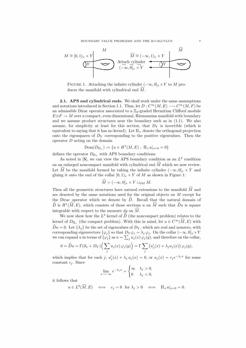
Figure 1. Attaching the infinite cylinder (−∞, 0]x×Y to M pro-

duces the manifold with cylindrical end M .

2.1. APS and cylindrical ends. We shall work under the same assumptionsand notations introduced in Section 1.1. Thus, letD : C∞(M,E) −→ C∞(M,F ) bean admissible Dirac operator associated to a Z2-graded Hermitian Clifford moduleE⊕F →M over a compact, even-dimensional, Riemannian manifold with boundaryand we assume product structures near the boundary such as in (1.1). We alsoassume, for simplicity at least for this section, that DY is invertible (which isequivalent to saying that it has no kernel). Let Π+ denote the orthogonal projectiononto the eigenspaces of DY corresponding to the positive eigenvalues. Then theoperator D acting on the domain

Dom(DΠ+) := u ∈ H1(M,E) ; Π+u|x=0 = 0

defines the operator DΠ+with APS boundary conditions.

As noted in [5], we can view the APS boundary condition as an L2 condition

on an enlarged noncompact manifold with cylindrical end M which we now review.

Let M be the manifold formed by taking the infinite cylinder (−∞, 0]x × Y andgluing it onto the end of the collar [0, 1)x × Y of M as shown in Figure 1:

M = (−∞, 0]x × Y t∂M M.

Then all the geometric structures have natural extensions to the manifold M andare denoted by the same notations used for the original objects on M except for

the Dirac operator which we denote by D. Recall that the natural domain of

D is H1(M,E), which consists of those sections u on M such that Du is square

integrable with respect to the measure dg on M .

We now show how the L2 kernel of D (the noncompact problem) relates to the

kernel of DΠ+(the compact problem). With this in mind, let u ∈ C∞(M,E) with

Du = 0. Let λj be the set of eigenvalues of DY , which are real and nonzero, withcorresponding eigenvectors ϕj so that DY ϕj = λj ϕj . On the collar (−∞, 0]x×Ywe can expand u in terms of ϕj as u =

∑j uj(x)ϕj(y), and therefore on the collar,

0 = Du = Γ(∂x +DY )( ∑

j

uj(x)ϕj(y))

= Γ∑

j

(u′j(x) + λjuj(x)

)ϕj(y),

which implies that for each j, u′j(x) + λj uj(x) = 0, or uj(x) = cje−λjx for some

constant cj . Since

limx→−∞

e−λjx =

∞ λj > 0,

0 λj < 0,

it follows that

u ∈ L2(M,E) ⇐⇒ cj = 0 for λj > 0 ⇐⇒ Π+u|x=0 = 0.

8 PAUL LOYA

Thus,

(2.1) ker D ∼= kerDΠ+,

where the left-hand side is the kernel of D on its natural domain. Similarly, one

can show that the kernels of the adjoints are isomorphic: ker D∗ ∼= kerD∗Π+

.

Before stating the APS index theorem for the operators D and DΠ+, we go into

more depth on the eta invariant than was described in Section 1.2. The originalway to define the eta invariant was through the eta function, η(z), which is definedas the meromorphic function

(2.2) η(z) =∑

j

signλj|λj |z

.

In the general case when DY has a kernel, we only sum over λj 6= 0. Weyl asymp-totics show that η(z) is holomorphic for Re z > dimY , but one of the main accom-plishments of [5] was the proof that η(z) in fact defines a meromorphic function onC that is regular at z = 0. The eta invariant of DY is the value of the eta functionat zero, η(DY ) = η(0), which represents a formal signature of the operator DY :

“ η(DY ) =∑

j

signλj|λj |z

∣∣∣∣z=0

=∑

j

signλj = #λj > 0 − #λj < 0. ”

The reason for the quotation marks is that there are an infinite number of positiveand negative eigenvalues, so this equation really reads ∞−∞! Nonetheless, η(DY )can be interpreted as a measurement of the signature or spectral asymmetry of DY .We can also express the eta function in terms of the heat operator via

(2.3) η(z) =1

Γ( z+12 )

∫ ∞

0

tz−1

2 Tr(DY e−tD2

Y ) dt,

where Γ(z) is the Gamma function. To see this, we notice that

Tr(DY e−tD2

Y ) =∑

j

λj e−tλ2

j

and that

1

Γ( z+12 )

∫ ∞

0

tz−1

2 λj e−tλ2

j dt =λj

|λj |z+1· 1

Γ( z+12 )

∫ ∞

0

tz−1

2 e−t dt =signλj|λj |z

,

where we made the change of variables t 7→ t/|λj |2. In particular, according to [6],we can set z = 0 in (2.3) to obtain the following important formula:

(2.4) η(DY ) =1√π

∫ ∞

0

t−1/2 Tr(DY e−tD2

Y ) dt.

The advantage of this formula is that it naturally falls out of the heat kernel proofof the APS index formula as we shall see in Section 2.5.

We are now ready to state the (simplified) Atiyah-Patodi-Singer index theorem,which is a special case of Theorem 1.1 when DY is invertible, and hence V = kerDY

is just the zero vector space. The following statement is not how their theoremoriginally appeared, but all its content were part of the original paper [5].

Theorem 2.1. Let D be a Dirac operator on an even-dimensional, compact,oriented, Riemannian manifold with boundary with product type structures specifiedas in Section 1.1 and such that the boundary operator DY is invertible. Then

BOUNDARY VALUE PROBLEMS AND THE B-CALCULUS 9

(a) ker D ∼= kerDΠ+and ker D∗ ∼= kerD∗

Π+.

(b) The operators

D : H1(M,E) −→ L2(M, F ),

DΠ+: Dom(DΠ+

) −→ L2(M,F )

are Fredholm with (by (a)) equal indices.(c) The following index formula holds:

ind D = indDΠ+=

∫AS − 1

2η(DY ).

We already proved Part (a) around (2.1). For Part (b), the Fredholm property

of D follows from Lemma 2.3 below; for the Fredholm properties of DΠ+, see [5] or

Booß-Bavnbek and Wojciechowski [10]. We shall prove Part (c) in Section 2.5. Todo so, we use the machinery of Melrose’s b-calculus [40] which we describe next.

2.2. b-pseudodifferential operators. We only describe the so-called “smallover-blown” calculus of b-pseudodifferential operators. There are also “big” calculiwhich are useful for establishing Fredholm properties of b-pseudodifferential oper-ators or for obtaining precise information concerning Green operators, but for thegoals of this paper, these larger calculi are unnecessary.

So what exactly is a b-pseudodifferential operator? Perhaps the best way tothink of a b-pseudodifferential operator is as a usual pseudodifferential operator on

M that is exponentially uniform as x → −∞ on the cylindrical end. As with allalgebras of operators defined on noncompact manifolds, cf. Lockhart and McOwen[30], Rabinovic [51], and Schrohe [53], we need to have control in asymptoticbehavior at infinity in order to get a well-behaved class of operators. This is nodifferent in our situation, where we require “exponential asymptotics”. Therefore,before describing the small calculus, we need to fix the notion of exponential decay.Later, we shall see that these conditions can be interpreted quite naturally as C∞

conditions on a related compact manifold.We say that a smooth function u(x, y) on the infinite cylinder (−∞, 0]x × Y

can be expanded exponentially on the cylindrical end if

(2.5) u(x, y) ∼∞∑

k=0

ekx uk(y) = u0(y) + ex u1(y) + e2x u2(y) + · · · ,

where uk ∈ C∞(Y ) for each k. This asymptotic sum means that for any N ,

(2.6) u(x, y) −N−1∑

k=0

ekx uk(y) = eNx rN (x, y),

where all derivatives of the remainder rN (x, y) in x and y are bounded. In par-ticular, u(x, y) = u0(y) modulo an exponentially decaying term. We say that uvanishes to infinite exponential order on the cylindrical end if u can be expandedexponentially as x → −∞ with all the uk(y)’s zero; equivalently, u with all itsderivatives vanish faster on the cylindrical end than any exponential power.

Let S(M) denote the set of all smooth functions on M that vanish to infiniteexponential order on the cylindrical end. A b-pseudodifferential operator A of order

m ∈ R is a continuous linear map on S(M) that has the following properties: Given

any compactly supported ψ ∈ C∞c (M) equal to 1 on M , and smooth ϕ ∈ C∞(M)

10 PAUL LOYA

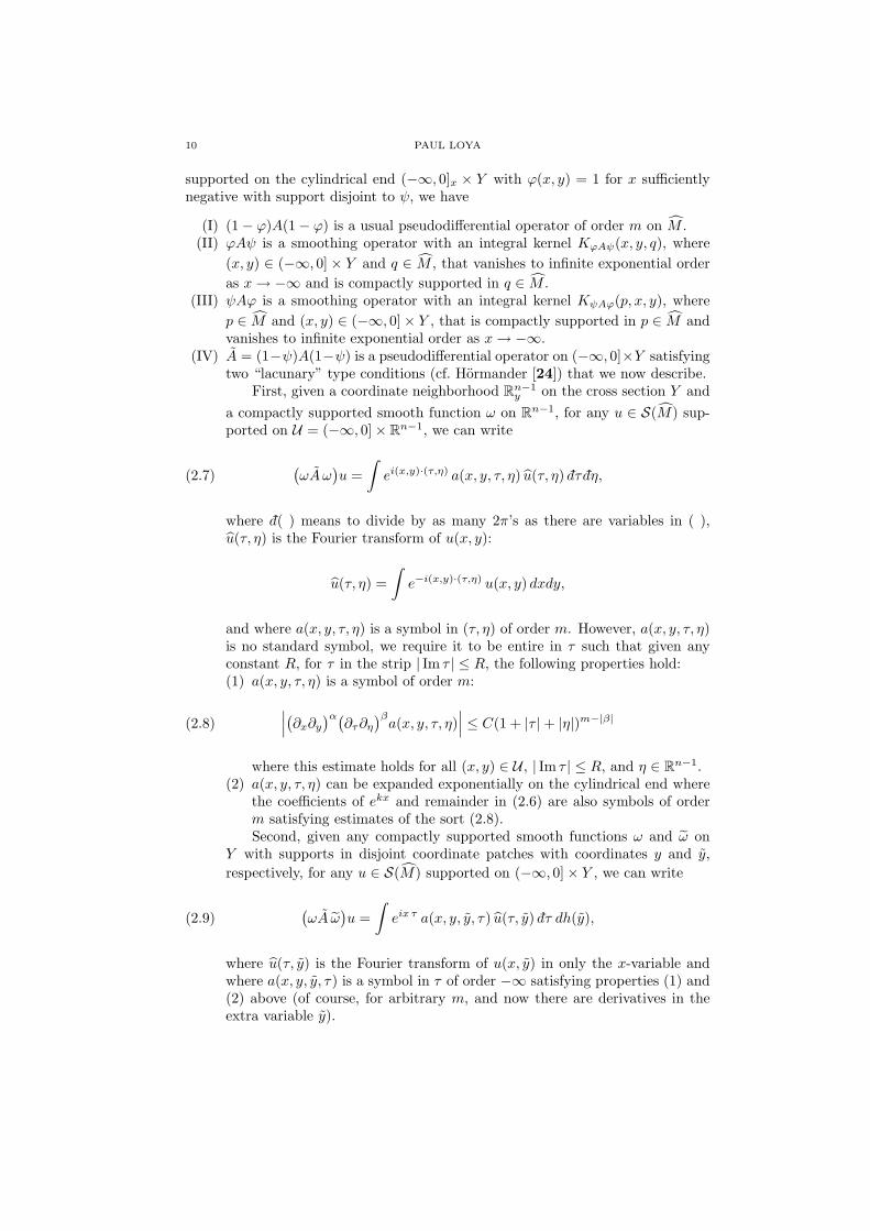
supported on the cylindrical end (−∞, 0]x × Y with ϕ(x, y) = 1 for x sufficientlynegative with support disjoint to ψ, we have

(I) (1 − ϕ)A(1 − ϕ) is a usual pseudodifferential operator of order m on M .(II) ϕAψ is a smoothing operator with an integral kernel KϕAψ(x, y, q), where

(x, y) ∈ (−∞, 0] × Y and q ∈ M , that vanishes to infinite exponential order

as x→ −∞ and is compactly supported in q ∈ M .(III) ψAϕ is a smoothing operator with an integral kernel KψAϕ(p, x, y), where

p ∈ M and (x, y) ∈ (−∞, 0] × Y , that is compactly supported in p ∈ M andvanishes to infinite exponential order as x→ −∞.

(IV) A = (1−ψ)A(1−ψ) is a pseudodifferential operator on (−∞, 0]×Y satisfyingtwo “lacunary” type conditions (cf. Hormander [24]) that we now describe.

First, given a coordinate neighborhood Rn−1y on the cross section Y and

a compactly supported smooth function ω on Rn−1, for any u ∈ S(M) sup-ported on U = (−∞, 0] × Rn−1, we can write

(2.7)(ωAω

)u =

∫ei(x,y)·(τ,η) a(x, y, τ, η) u(τ, η) dτ dη,

where d( ) means to divide by as many 2π’s as there are variables in ( ),u(τ, η) is the Fourier transform of u(x, y):

u(τ, η) =

∫e−i(x,y)·(τ,η) u(x, y) dxdy,

and where a(x, y, τ, η) is a symbol in (τ, η) of order m. However, a(x, y, τ, η)is no standard symbol, we require it to be entire in τ such that given anyconstant R, for τ in the strip | Im τ | ≤ R, the following properties hold:(1) a(x, y, τ, η) is a symbol of order m:

(2.8)∣∣∣(∂x∂y

)α(∂τ∂η

)βa(x, y, τ, η)

∣∣∣ ≤ C(1 + |τ | + |η|)m−|β|

where this estimate holds for all (x, y) ∈ U , | Im τ | ≤ R, and η ∈ Rn−1.(2) a(x, y, τ, η) can be expanded exponentially on the cylindrical end where

the coefficients of ekx and remainder in (2.6) are also symbols of orderm satisfying estimates of the sort (2.8).Second, given any compactly supported smooth functions ω and ω on

Y with supports in disjoint coordinate patches with coordinates y and y,

respectively, for any u ∈ S(M) supported on (−∞, 0] × Y , we can write

(2.9)(ωA ω

)u =

∫eix τ a(x, y, y, τ) u(τ, y) dτ dh(y),

where u(τ, y) is the Fourier transform of u(x, y) in only the x-variable andwhere a(x, y, y, τ) is a symbol in τ of order −∞ satisfying properties (1) and(2) above (of course, for arbitrary m, and now there are derivatives in theextra variable y).

BOUNDARY VALUE PROBLEMS AND THE B-CALCULUS 11

The set of all such operators is denoted3 by Ψmb (M). A b-smoothing operator

is a b-pseudodifferential operator of order −∞. Just like the usual class of pseu-dodifferential operators on compact manifolds without boundary, the space of allb-pseudodifferential operators forms a ∗-filtered algebra of operators with the filtra-tion determined by the principal symbol. One can also define a corresponding spaceof classical operators. See [40] for more information. Also, there exist natural

Sobolev spaces Hs(M) on M with H0(M) = L2(M) and if A ∈ Ψmb (M), then A

defines a continuous linear map,

(2.10) A : Hs(M) −→ Hs−m(M).

We now describe the normal operator, which captures the dominant behavior

of A ∈ Ψmb (M) as x→ −∞. Let a0(y, τ, η) be the first term in the expansion (2.5)

for b(x, y, τ, η) on the cylindrical end. Then b(x, y, τ, η) = a0(y, τ, η) modulo anexponentially decaying term as x → −∞. The normal or indicial operator of A isthe entire family N(A)(τ) ∈ Ψm(Y ) defined locally by

(2.11) N(A)(τ)ψ =

∫eiy·η a0(y, τ, η) ψ(η) dη;

there is a similar formula in disjoint coordinate patches using (2.9). The normaloperator preserves composition:

N(AB)(τ) = N(A)(τ) N(B)(τ)

and in a certain respect, adjoints:

N(A∗)(τ) = N(A)(τ)∗,

where τ is the complex conjugate of τ . Finally, we remark that the normal operatorgoverns the Fredholm properties of b-pseudodifferential operators, see Mazzeo [35],Melrose [40], or Loya and Melrose [33]:

Theorem 2.2. Let A ∈ Ψmb (M) with m ∈ R. Then

A : Hm(M) −→ L2(M)

is Fredholm if and only if A is elliptic and for all τ ∈ R,

N(A)(τ) : Hm(Y ) −→ L2(Y )

is invertible.

Of course, everything that we have said so far for operators on functions worksequally well for operators mapping between sections of vector bundles. We nowconsider the Dirac operator, our main example of a b-pseudodifferential operator.

In this case, it is easy to see that D is a first order b-pseudodifferential operator.

Indeed, since D = Γ(∂x +DY ) on the cylinder, given any u supported on a coordi-nate patch with local coordinates (x, y), writing u as the inverse Fourier transform

3This space usually has a subscript “ob”, Ψm

ob(M), for “over-blown.” When the cross section

Y is disconnected, this is a slightly larger class of operators than described by Melrose in [40];

when Y is connected, this over-blown space is exactly the same as in loc. cit. Finally, we remark

that “over-blown” has to do with the blown-up space X2b

to be described in Section 2.3.

12 PAUL LOYA

of its Fourier transform, we have

Du(x, y) = Γ(∂x +DY )

∫ei(x,y)·(τ,η) u(τ, η) dτ dη

=

∫ei(x,y)·(τ,η) Γ(iτ + b(y, η)) u(τ, η) dτ dη,

where b(y, η) = DY

(eiy·η

)is the symbol of DY in local coordinates. The function

Γ(iτ + b(y, η)) is certainly a symbol of order 1 satisfying all of (1) and (2) around

(2.8). Thus, D ∈ Ψ1b(M,E, F ). Moreover, by definition of the normal operator

(2.11),

N(D)(τ)ψ =

∫eiy·η Γ(iτ + b(y, η)) ψ(η) dη = Γ(iτ +DY )ψ.

Thus,

(2.12) N(D)(τ) = Γ(iτ +DY ),

a formula that we shall use later in our proof of the APS theorem. Let EY = E|x=0

and FY = F |x=0. Since DY is self-adjoint,

iτ +DY : Hm(Y,EY ) −→ L2(Y,EY )

is automatically invertible for τ 6= 0 and is invertible at τ = 0 if and only if DY isinvertible. It follows that

N(D)(τ) = Γ(iτ +DY ) : Hm(Y,EY ) −→ L2(Y, FY )

is invertible for all τ ∈ R if and only if DY is invertible. Although we have beenworking under the even-dimensional assumption, this whole argument works for anydimensional manifold. Thus, Theorem 2.2 immediately gives the following theorem,which proves the first part in Part (b) of Theorem 2.1.

Lemma 2.3. Let D be a Dirac operator on a compact Riemannian manifold

with boundary with product type structures near the boundary. Then D is Fredholmon its natural (that is, Sobolev) domain if and only if DY is invertible.

Of course, in this section we have been assuming that DY is invertible, but theproof of this lemma does not require this assumption.

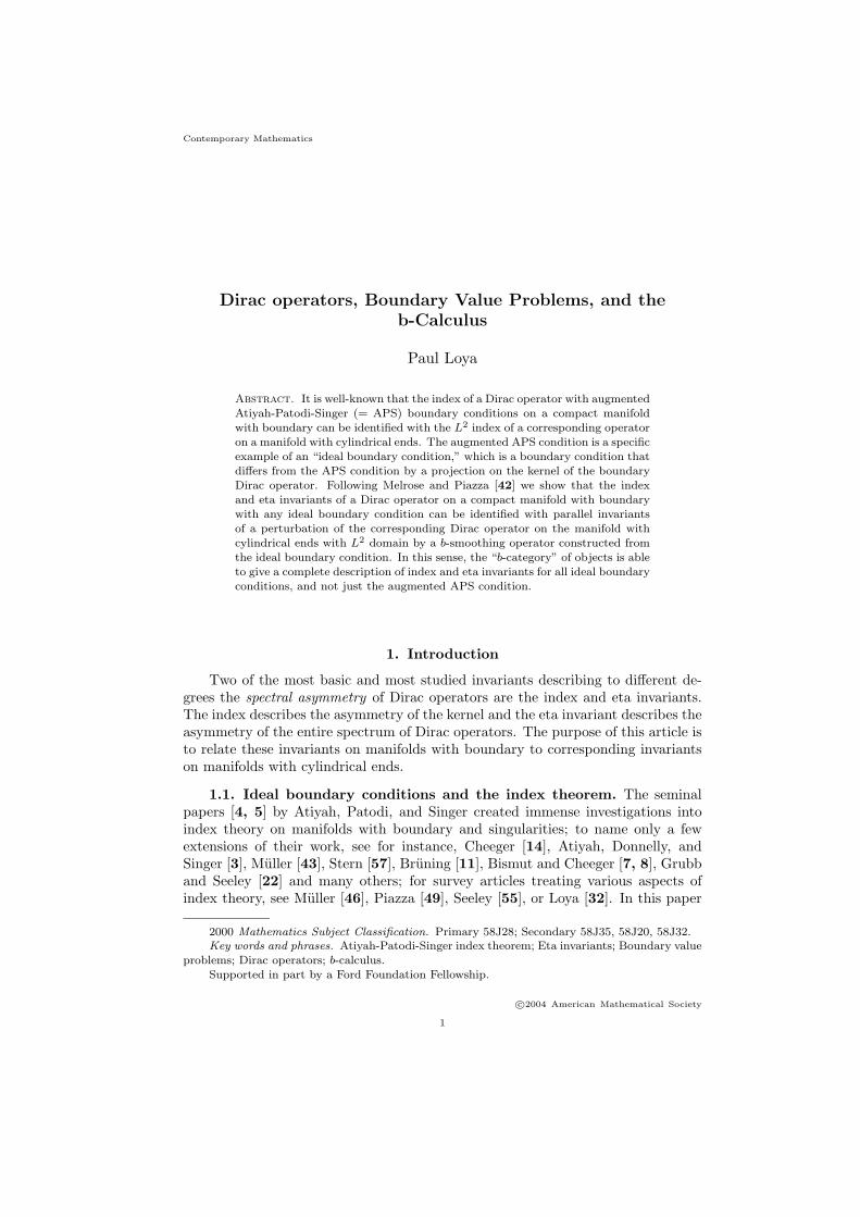
2.3. The compact picture. Now what is all this stuff about exponentialasymptotics? Isn’t there a more natural way to describe these operators? There issuch a way, which we now explain. First we need to make a simple campactification

of our noncompact manifold M . On the cylindrical end (−∞, 0]x×Y of M we makethe change of variables r = ex. Notice that as x → −∞, r → 0. Thus, under this

change of variables, M transforms into the interior of the compact manifold with

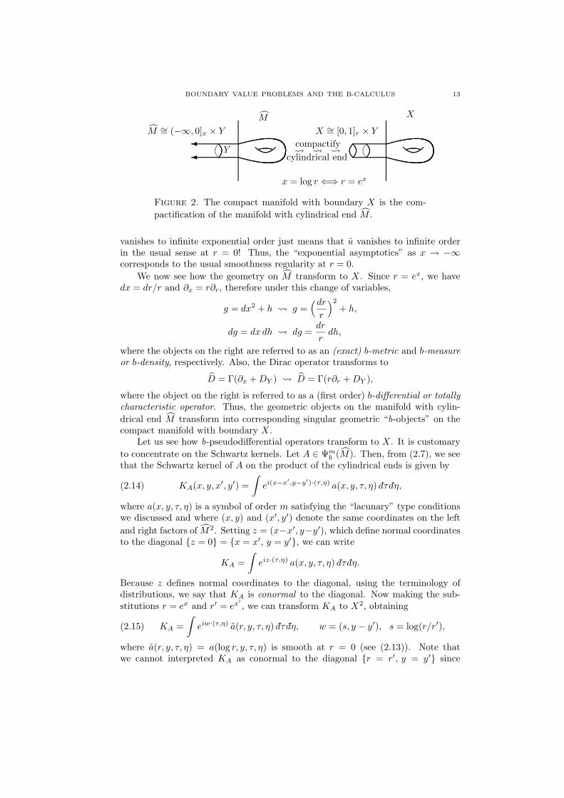
boundary X, where X has the same compact end as M but with the cylindricalend (−∞, 0]x × Y replaced with the compact end [0, 1]r × Y , see Figure 2.

Observe that under the change of variables r = ex, the asymptotic expansion(2.5) transforms to

(2.13) u(x, y) ∼∞∑

k=0

ekx uk(y) u(r, y) ∼∞∑

k=0

rk uk(y), u(r, y) = u(log r, y);

in other words, u(r, y) is smooth in the usual sense at r = 0! (We do have to thinka little about the remainders in (2.6), but this is not difficult.) In particular, u

BOUNDARY VALUE PROBLEMS AND THE B-CALCULUS 13

compactify

cylindrical end

Y

M

M ∼= (−∞, 0]x × Y X ∼= [0, 1]r × Y

X

x = log r ⇐⇒ r = ex

Figure 2. The compact manifold with boundary X is the com-

pactification of the manifold with cylindrical end M .

vanishes to infinite exponential order just means that u vanishes to infinite orderin the usual sense at r = 0! Thus, the “exponential asymptotics” as x → −∞corresponds to the usual smoothness regularity at r = 0.

We now see how the geometry on M transform to X. Since r = ex, we havedx = dr/r and ∂x = r∂r, therefore under this change of variables,

g = dx2 + h g =(drr

)2

+ h,

dg = dx dh dg =dr

rdh,

where the objects on the right are referred to as an (exact) b-metric and b-measureor b-density, respectively. Also, the Dirac operator transforms to

D = Γ(∂x +DY ) D = Γ(r∂r +DY ),

where the object on the right is referred to as a (first order) b-differential or totallycharacteristic operator. Thus, the geometric objects on the manifold with cylin-

drical end M transform into corresponding singular geometric “b-objects” on thecompact manifold with boundary X.

Let us see how b-pseudodifferential operators transform to X. It is customary

to concentrate on the Schwartz kernels. Let A ∈ Ψmb (M). Then, from (2.7), we see

that the Schwartz kernel of A on the product of the cylindrical ends is given by

(2.14) KA(x, y, x′, y′) =

∫ei(x−x

′,y−y′)·(τ,η) a(x, y, τ, η) dτ dη,

where a(x, y, τ, η) is a symbol of order m satisfying the “lacunary” type conditionswe discussed and where (x, y) and (x′, y′) denote the same coordinates on the left

and right factors of M2. Setting z = (x−x′, y−y′), which define normal coordinatesto the diagonal z = 0 = x = x′, y = y′, we can write

KA =

∫eiz·(τ,η) a(x, y, τ, η) dτ dη.

Because z defines normal coordinates to the diagonal, using the terminology ofdistributions, we say that KA is conormal to the diagonal. Now making the sub-stitutions r = ex and r′ = ex

′

, we can transform KA to X2, obtaining

(2.15) KA =

∫eiw·(τ,η) a(r, y, τ, η) dτ dη, w = (s, y − y′), s = log(r/r′),

where a(r, y, τ, η) = a(log r, y, τ, η) is smooth at r = 0 (see (2.13)). Note thatwe cannot interpreted KA as conormal to the diagonal r = r′, y = y′ since

14 PAUL LOYA

r′

r

r = r′

CCO “blow up” r = r′ = 0

X2

s = log( r

r′) = log cot θ

kU

s < 0

s > 0ff

lb = s = −∞

rb = s = ∞

s = 0

logarithmic projective coordinates

X2

b

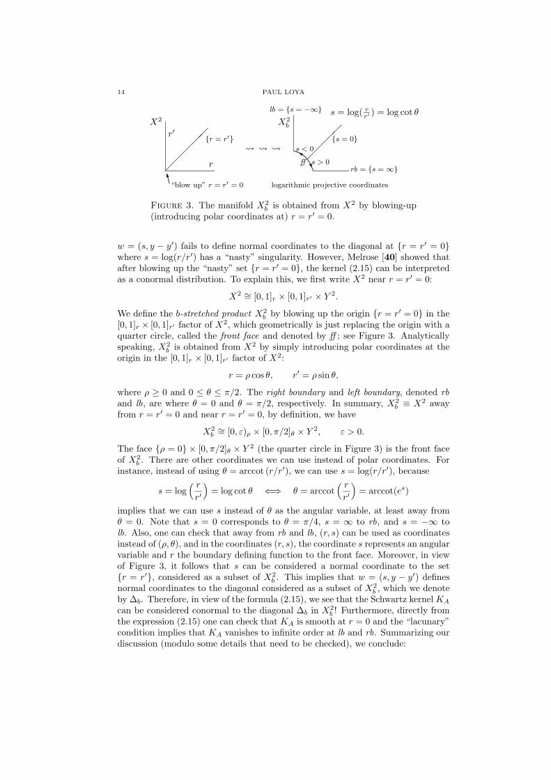
Figure 3. The manifold X2b is obtained from X2 by blowing-up

(introducing polar coordinates at) r = r′ = 0.

w = (s, y − y′) fails to define normal coordinates to the diagonal at r = r′ = 0where s = log(r/r′) has a “nasty” singularity. However, Melrose [40] showed thatafter blowing up the “nasty” set r = r′ = 0, the kernel (2.15) can be interpretedas a conormal distribution. To explain this, we first write X2 near r = r′ = 0:

X2 ∼= [0, 1]r × [0, 1]r′ × Y 2.

We define the b-stretched product X2b by blowing up the origin r = r′ = 0 in the

[0, 1]r × [0, 1]r′ factor of X2, which geometrically is just replacing the origin with aquarter circle, called the front face and denoted by ff ; see Figure 3. Analyticallyspeaking, X2

b is obtained from X2 by simply introducing polar coordinates at theorigin in the [0, 1]r × [0, 1]r′ factor of X2:

r = ρ cos θ, r′ = ρ sin θ,

where ρ ≥ 0 and 0 ≤ θ ≤ π/2. The right boundary and left boundary, denoted rband lb, are where θ = 0 and θ = π/2, respectively. In summary, X2

b ≡ X2 awayfrom r = r′ = 0 and near r = r′ = 0, by definition, we have

X2b∼= [0, ε)ρ × [0, π/2]θ × Y 2, ε > 0.

The face ρ = 0 × [0, π/2]θ × Y 2 (the quarter circle in Figure 3) is the front faceof X2

b . There are other coordinates we can use instead of polar coordinates. Forinstance, instead of using θ = arccot (r/r′), we can use s = log(r/r′), because

s = log( rr′

)= log cot θ ⇐⇒ θ = arccot

( rr′

)= arccot(es)

implies that we can use s instead of θ as the angular variable, at least away fromθ = 0. Note that s = 0 corresponds to θ = π/4, s = ∞ to rb, and s = −∞ tolb. Also, one can check that away from rb and lb, (r, s) can be used as coordinatesinstead of (ρ, θ), and in the coordinates (r, s), the coordinate s represents an angularvariable and r the boundary defining function to the front face. Moreover, in viewof Figure 3, it follows that s can be considered a normal coordinate to the setr = r′, considered as a subset of X2

b . This implies that w = (s, y − y′) definesnormal coordinates to the diagonal considered as a subset of X2

b , which we denoteby ∆b. Therefore, in view of the formula (2.15), we see that the Schwartz kernel KA

can be considered conormal to the diagonal ∆b in X2b ! Furthermore, directly from

the expression (2.15) one can check that KA is smooth at r = 0 and the “lacunary”condition implies that KA vanishes to infinite order at lb and rb. Summarizing ourdiscussion (modulo some details that need to be checked), we conclude:

BOUNDARY VALUE PROBLEMS AND THE B-CALCULUS 15

Geometric definition: Ψmb (M) consists of operators whose

Schwartz kernels are distributions onX2b conormal to ∆b, smooth

at ff , and vanishing to infinite order at lb and rb.

In this paper we shall work with M leaving the interested reader to check outMelrose [40] or Mazzeo [35] for this conormal distribution viewpoint.

2.4. The b-trace. We now introduce the star of the show: The b-trace. By

(2.10) any A ∈ Ψ−∞b

(M) defines a continuous linear map

A : L2(M) −→ L2(M),

but we note that this map is in general not trace class (or even compact). Theb-trace is designed to make b-smoothing operators (b-pseudodifferential operatorsof order −∞) trace-class even though they are really not trace-class! Indeed, wewould like to define the trace of A via a Lidskiı type formula, cf. [28]:

“ Tr(A) =

∫

M

KA|∆, ”

where KA denotes the Schwartz kernel of A and ∆ is the diagonal in M × M and

we make the identification M ≡ ∆. The reason for the quotation marks is thatthis integral does not exist because the integral over the cylindrical end actuallydiverges (in general)! To see this, note that by the definition of b-pseudodifferentialoperators, in coordinates (x, y) on the cylindrical end we can write

(2.16) KA|∆ = a0(y) + a1(x, y),

where both a0 and a1 are smooth and a1(x, y) decays like ex as x→ −∞. Therefore,

since∫ 0

−∞ dx diverges, the integral∫

M

KA|∆ =

∫

(−∞,0]x×YKA|∆ dx dh+

∫

M

KA|∆

=

∫

(−∞,0]x×Ya0(y) dx dh+

∫

(−∞,0]x×Ya1(x, y) dx dh+

∫

M

KA|∆(2.17)

in general diverges since the first integral on the right does not exist in general,except of course when a0(y) = 0. This discussion shows that the function a0(y) isthe problem to the non-trace class nature of A. As we all know, one way to solvea problem is to simply get rid of it, and this is exactly what we shall do in oursituation: We throw out a0(y) in (2.17) to get a convergent integral, which we callthe b-trace of A:

bTrA :=

∫

(−∞,0]x×Ya1(x, y) dx dh+

∫

M

KA|∆.

In particular, if a0(y) = 0, which happens if A vanishes exponentially at the end ofthe cylinder, then KA|∆ = a1(x, y) on the cylinder, so in this case bTrA equals

∫

(−∞,0]x×YKA|∆ dx dh+

∫

M

KA|∆ =

∫

M

KA|∆,

the trace of A in the usual sense. In the following lemma we show how the b-traceis related to elementary complex analysis.

16 PAUL LOYA

Lemma 2.4. Let A ∈ Ψ−∞b (M). Then for all complex numbers z with Re z > 0,

the operator ezxA is trace class and the integral

F (z) =

∫

M

ezxKA|∆

exists. Moreover, F (z) extends from Re z > 0 to be a meromorphic function on thehalf-plane Re z > −1 with only a simple pole at z = 0.4 Furthermore, the regularvalue of F (z) at z = 0 is just the b-trace of A,

(2.18) bTrA = Regz=0 F (z),

and the residue of F (z) at z = 0 is given in terms of the normal operator of A via

(2.19) Resz=0 F (z) =1

2π

∫

R

Tr(N(A)(τ)) dτ.

Proof. Let Re z > 0. To see that ezxA is trace class, we write

(2.20) ezxA = ezx/2 ·(ezx/2Ae−zx/2

)· ezx/2.

Now the Schwartz kernel of A in local coordinates on the infinite cylinder is of theform, see (2.14)

(2.21) KA(x, y, x′, y′) =

∫ei(x−x

′,y−y′)·(τ,η) a(x, y, τ, η) dτ dη,

where the primes denote the same coordinates (x, y) but on the right factor of

M × M , and where a(x, y, τ, η) is a symbol of order −∞ satisfying properties (1)and (2) around (2.8). In these coordinates, it follows that the Schwartz kernel ofAz := ezx/2Ae−zx/2 is given by

KAz= ezx/2KA(x, y, x′, y′)e−zx

′/2 = e(x−x′)z/2KA

=

∫ei(x−x

′)(τ−iz/2)ei(y−y′)·η a(x, y, τ, η) dτ dη

=

∫ei(x−x

′)τei(y−y′)·η a(x, y, τ + iz/2, η) dτ dη,(2.22)

where we used the fact that the symbol is entire in τ . It follows that Az is also ab-smoothing operator. In view of (2.20), the Schwartz kernel of ezxA is given by

KezxA(x, y, x′, y′) = ezx/2 ·KAz· ezx′/2,

which vanishes exponentially like ezx/2 on the cylinders in both factors of M × M .Therefore, ezxA is trace class for Re z > 0.

We now verify the properties of F (z). Assuming that Re z > 0, the functionezx is integrable on (−∞, 0]x and for such z,

∫ 0

−∞ezx dx =

ezx

z

∣∣∣∣x=0

x=−∞=

1

z.

4It turns out that F (z) extends to be meromorphic on C with only simple poles at the points

0,−1,−2, . . ., but we don’t need this fact.

BOUNDARY VALUE PROBLEMS AND THE B-CALCULUS 17

Hence, writing KA|∆ as in (2.16), we see that

F (z) =

∫

M

ezxKA|∆

=

∫

(−∞,0]x×Yezx(a0(y) + a1(x, y)) dx dh+

∫

M

ezxKA|∆

=1

z

∫

Y

a0(y) dh+

∫

(−∞,0]x×Yezxa1(x, y) dx dh+

∫

M

ezxKA|∆,

where both a0 and a1 are smooth and a1(x, y) vanishes like ex as x → −∞. Itfollows that F (z) extends to be a meromorphic function on the strip Re z > −1,with regular value at z = 0 equal to bTrA, and with only a simple pole at z = 0with residue given by ∫

Y

a0(y) dh.

To show that this integral is related to the normal operator of A, observe thatsetting (x, y) = (x′, y′) in (2.21), we obtain

KA(x, y, x, y) =

∫a(x, y, τ, η) dτ dη,

so if a0(y, τ, η) is the limiting term in the expansion (2.5) for a(x, y, τ, η) as x→ −∞,then

(2.23)

∫

Y

a0(y) dh =

∫

Y

∫a0(y, τ, η) dτ dη dh(y).

On the other hand, by definition of N(A)(τ) (see (2.11)), we have

KN(A)(τ)(y, y′) =

∫ei(y−y

′)·η a0(y, τ, η) dη,

which implies that

(2.24) TrN(A)(τ) =

∫

Y

KN(A)(τ)(y, y) dh(y) =

∫

Y

∫a0(y, τ, η) dη dh(y).

Equating (2.23) and (2.24) proves (2.19) and completes the proof.

It is well-known that the trace functional on genuine (not b-) smoothing opera-tors on a compact manifold is the unique functional, up to multiplicative constant,that vanishes on commutators. The formula (2.25) below is sometimes called thetrace-defect formula because it gives a formula for the nonvanishing of the b-traceon commutators, and hence measures the “non-trace like nature” of the b-trace.

Theorem 2.5. If A ∈ Ψmb (M) and B ∈ Ψm′

b (M) with m+m′ = −∞, then

bTr[A,B] =i

2π

∫

R

Tr ( ∂τN(A)(τ) N(B)(τ) ) dτ(2.25)

= − i

2π

∫

R

Tr (N(A)(τ) ∂τN(B)(τ) ) dτ.

Proof. Integration by parts shows that the two integrals on the right areequal. Throughout this proof we assume that A is of order −∞ and we shall provethe first equality. To prove this theorem, we use Lemma 2.4, which states that

bTr[A,B] = Regz=0 Tr(ezx[A,B]).

18 PAUL LOYA

To evaluate the right-hand side, we first rewrite ezx[A,B] as

ezx[A,B] = [ezx, A]B + [A, ezxB].

Since the trace vanishes on commutators when one operator is a bounded operatorand the other is trace class, we have Tr([A, ezxB]) = 0 for Re z > 0, and hence itsanalytic continuation at z = 0 is zero also. Therefore, since

[ezx, A]B = ezx[AB − e−zxAezxB] = ezxAB −A(z)B,where A(z) = e−zxAezx, we have

(2.26) bTr[A,B] = Regz=0 Tr(ezxAB −A(z)B

).

Writing the Schwartz kernel of A as in (2.21) and using the same computationfound around (2.22), we can write the Schwartz kernel of A(z) as

KA(z) =

∫ei(x−x

′)τei(y−y′)·η a(x, y, τ − iz, η) dτ dη.

It follows that A(z) = e−zxAezx is also a b-pseudodifferential operator of order−∞ that is holomorphic in z such that A(0) = A. Moreover, if A′(z) denotes thederivative of A(z) with respect to z, then

KA′(z) = −i∫ei(x−x

′)τei(y−y′)·η ∂τa(x, y, τ − iz, η) dτ dη,

therefore, by definition of the normal operator,

(2.27) KN(A′(0))(τ) = −i∫ei(y−y

′)·η ∂τa(0, y, τ, η) dη = −iK∂τN(A)(τ).

Since A(0) = A, expanding A(z) in Taylor series at z = 0, we can write

AB −A(z)B = −zA′(0)B − z2C(z),

where C(z) is a b-smoothing operator that is holomorphic in z. In view of (2.26),we have

bTr[A,B] = −Regz=0

zTr(ezxA′(0)B) + z2 Tr(ezxC(z))

.

By Lemma 2.4, the traces on the right have at most simple poles at z = 0, so inparticular, the second term z2 Tr(ezxC(z)) vanishes at z = 0, while for the firstterm, by Lemma 2.4, we obtain

bTr[A,B] = −Regz=0 zTr(ezxA′(0)B) = −Resz=0 Tr(ezxA′(0)B)

= − 1

2π

∫

R

TrN(A′(0)B)(τ) dτ = − 1

2π

∫

R

Tr(N(A′(0))(τ)N(B)(τ)) dτ.

By (2.27), we see that N(A′(0))(τ) = −i∂τN(A)(τ), which finishes our proof.

2.5. The b-proof of the index theorem. We now give Melrose’s proof ofthe APS index formula in Theorem 2.1. For this we need the heat operators

e−tD∗D and e−tDD

∗

,

both of which exist via the usual arguments and moreover, are b-smoothing oper-ators for t > 0 (see Melrose [40] and Loya [31]). The key idea behind the heatkernel proof of the index formula is to consider the difference of the heat traces:

“ h(t) = Tr(e−tD∗D) − Tr(e−tDD

∗

). ”

BOUNDARY VALUE PROBLEMS AND THE B-CALCULUS 19

The reason for the quotation marks is that, as we observed earlier, b-smoothingoperators are in general not trace class; this is true in the present situation too forthe heat operators. However, the following b-object is well-defined:

h(t) = bTr(e−tD∗D) − bTr(e−tDD

∗

),

and we shall use this object instead of the ill-defined one above. We now indicatehow h(t) has the following amazing properties (however, we really only focus onProperty (3)):

(1) limt→∞

h(t) = ind D

(2) limt→0

h(t) =

∫

M

AS

(3) h′(t) = − 1

2√πt−1/2Tr(DY e

−tD2Y ).

These three facts together with the basic fundamental theorem of calculus easilyprove the APS formula:

ind D = h(∞) = h(0) +

∫ ∞

0

h′(t) dt

=

∫

M

AS +

∫ ∞

0

− 1

2√πt−1/2Tr(DY e

−tD2Y ) dt

=

∫

M

AS − 1

2√π

∫ ∞

0

t−1/2Tr(DY e−tD2

Y ) dt

=

∫

M

AS − 1

2η(DY ).

It turns out that the proofs of Property (1) and Property (2) follow basicallythe same lines of reasoning as for the corresponding statements in the compactmanifold without boundary case. For this reason, we shall not discuss them indetail and leave the reader to check Chapters 8 and 9 in [40] for the arguments.However, we remark that Property (2) follows from the the so-called local index

theorem, which states that for p ∈ M ,

limt→0

tr e−tD

∗D(p, p) − tr e−tDD∗

(p, p)

= AS(p)

uniformly in t, where the lower case tr denotes the fiber-wise trace, and where theright-hand side really represents the coefficient of the volume form component ofthe differential form AS(p), cf. McKean and Singer [38], Gilkey [19], Patodi [48],Alvarez-Gaume [1], and Getzler [18]. Note that AS vanishes on the cylindrical endby our product type hypothesis.

We now prove (3), which is where we see our hero, the b-trace, in action inthe direct manner by which (3) is derived. First, recalling the elementary identity5

5This identity follows from uniqueness of solutions to the heat equation, cf. [40, p. 271].

20 PAUL LOYA

D∗De−tD∗D = D∗e−tDD

∗

D, we take the derivative of h(t):

h′(t) =d

dt

(bTr(e−tD

∗D) − bTr(e−tDD∗

))

= bTr(−D∗De−tD∗D ) + bTr( DD∗e−tDD

∗

)

= bTr(−D∗e−tDD∗

D ) + bTr( DD∗e−tDD∗

)

= bTr( [D, D∗e−tDD∗

] ),

(2.28)

where [D, D∗e−tDD∗

] is the commutator of D and D∗e−tDD∗

. Second, by thetrace-defect formula, we find

h′(t) = bTr( [D, D∗e−tDD∗

] )

=i

2π

∫

R

Tr(∂τN(D)(τ)N(D∗)(τ)N(e−tDD

∗

)(τ))dτ.

Third, we complete the verification of (3) by directly computing the right-hand side

of h′(t) to equal − 12√πt−1/2Tr(DY e

−tD2Y ). To see this, observe that for τ ∈ R, by

the formula (2.12) for the normal operator of D, we have

N(D)(τ) = Γ(iτ +DY ) and N(D∗)(τ) = −(−iτ +DY )Γ∗.

It follows that

N(DD∗)(τ) = N(D)(τ)N(D∗)(τ) = Γ(τ2 +D2Y )Γ∗.

Now it is easily proved from the continuity properties of the normal operator that

N(e−tDD∗

)(τ) = e−tN(DD∗)(τ) = Γe−tτ2

e−tD2Y Γ∗.

Multiplying this with ∂τN(D)(τ) = iΓ and N(D∗)(τ), we obtain

∂τN(D)(τ)N(D∗)(τ)N(e−tDD∗

)(τ) = iΓ(−iτ +DY )e−tτ2

e−tD2Y Γ∗.

Finally, using the facts that∫

Rτe−tτ

2

dτ = 0,∫

Re−tτ

2

dτ = t−1/2√π, and Γ is

unitary, we get our desired result:

h′(t) = bTr( [D, D∗e−tDD∗

] ) =i

2π

∫

R

Tr(∂τN(D)(τ)N(D∗)(τ)N(e−tDD

∗

)(τ))dτ

=i

2π

∫

R

Tr( iΓ(−iτ +DY )e−tτ2

e−tD2Y Γ∗ ) dτ

=i2

2πt−1/2

√π Tr(DY e

−tD2Y ).

= − 1

2√πt−1/2 Tr(DY e

−tD2Y ).

3. Transformation to b-objects II

In this section we prove Theorem 1.1. Needless to say, we now drop all as-sumptions about the invertibility of DY . We start this section by defining the b-

smoothing perturbation T in Theorem 1.1 and then we relate the kernels of D− Tand DT . One of the main goals in this section is to prove the general index theorem3.4 from which the index formula in Theorem 1.1 follows. The direct (but somewhatcomplicated) computation of the eta invariant portion of the general index formula

BOUNDARY VALUE PROBLEMS AND THE B-CALCULUS 21

(3.8) boils down once again to the trace-defect formula. We end this section byproving this general index formula.

3.1. Definition of T . We begin by defining the b-smoothing perturbation T

in Theorem 1.1. Let D and D be as in Section 1.1 and let T be a self-adjointisomorphism on V = kerDY with T 2 = Id.

The b-smoothing operator T is really very simple to define. First, we define anauxiliary b-smoothing operator on the half-line (−∞, 0]. Let χ ∈ C∞(R), whereχ(x) = 1 for x ≤ −2 and χ(x) = 0 for x ≥ −1. Let ϕ ≥ 0 be a smooth compactlysupported even function on R with ϕ(0) > 0. Then ϕ(τ) is an even entire function.Define Q ∈ Ψ−∞

b ((−∞, 0]) by

(3.1) Qu = χ(x)

∫

R

eixτ ϕ(τ) χu(τ) dτ,

where χu is the Fourier transform of χu:

χu(τ) =

∫

R

e−ixτ χ(x)u(x) dx.

The Schwartz kernel of Q is

KQ = χ(x) ·∫

R

ei(x−x′)τ ϕ(τ) dτ · χ(x′).

Since ϕ is compactly supported, ϕ(τ) vanishes to infinite order as |τ | → ∞ for| Im τ | within any fixed bound and therefore, Q ∈ Ψ−∞

b ((−∞, 0]) by definition of

this space. Moreover, since ϕ is even, ϕ(τ) is also even, so KQ(x, x′) = KQ(x′, x),which implies that Q is self-adjoint. Finally, by definition of the normal operator,we have

N(Q)(τ) = ϕ(τ).

Second, we note that T is a smoothing operator. To see this, observe that wecan identify T : V −→ V with T π : L2(Y,EY ) −→ V , with π the orthogonalprojection of L2(Y,EY ) onto V . Since V ⊂ C∞(Y,EY ) is finite dimensional itfollows that T is a (finite rank) smoothing operator.

Third, we define the b-smoothing operator T ∈ Ψ−∞b (M,E, F ) supported on

the cylindrical end (−∞, 0]x × Y by

(3.2) T = ΓQ2T ∈ Ψ−∞b (M,E, F ),

where Q is the self-adjoint operator given in (3.1). Note that T acts on the crosssection Y while Q acts on the cylinder part (−∞, 0]x, and Γ simply maps E to F .

The normal operator of T is given by

(3.3) N(T )(τ) = N(ΓQ2T )(τ) = ΓN(Q)(τ)2T = Γ ϕ(τ)2T.

Now to the proof of Theorem 1.1. We shall prove Property (a) of Theorem 1.1in Section 3.2 and then Properties (b) and (c) in Section 3.3.

3.2. Relation of kernels and indices of D− T and DT . Throughout this

section we denote the +1 eigenspace of T by ΛT . To prove that ker(D−T ) ∼= kerDT

and ker(D − T )∗ ∼= kerD∗T , we start off with the following lemma.

22 PAUL LOYA

Lemma 3.1. If T is a self-adjoint linear map on V and W is a subspace of V ,then given any v0 ∈W , the boundary value problem

v ∈ H1((−∞, 0], V ),(∂x −Q2T

)v = 0, v|x=1 = v0,

has a non-trivial solution if and only if v0 ∈ ΛT ∩W , in which case, the solution isunique and also takes values in ΛT ∩W .

Proof. We can decompose ΛT as ΛT = U0 ⊕ U1, where U0 = ΛT ∩W andU1 is the orthogonal complement in ΛT of U0. Thus, we can decompose the vectorspace V and matrix T as

V = U0 ⊕ U1 ⊕ Λ⊥T , T = Id ⊕ Id ⊕−Id.

Since we can decompose any element of H1((−∞, 0], V ) into functions taking valuesin U0, U1, and Λ⊥

T , our lemma is proved once we show that there are exactly dim(U0)non-trivial solutions to the boundary value problem

(3.4) v ∈ H1((−∞, 0], V ),(∂x −Q2T

)v = 0, v|x=1 ∈W

if v takes values in U0, and has no solutions otherwise. First suppose that v takesvalues in Λ⊥

T . Since T = −1 on Λ⊥T , we have

(3.5)(∂x +Q2

)v(x) = 0.

By choosing a basis for W , we may assume that v is a scalar function. Also, since∂x and Q are real, we may assume that v is a real-valued function. Since v is an L2

solution of (3.5), elementary use of the Fourier transform can be used to show that

v(x) → 0 as x → −∞. This implies that∫ 0

−∞ v′ vdx = 12v(0)2. Thus, multiplying

(3.5) by v dx, integrating from −∞ to 0, and using that Q is self-adjoint, we obtain

(3.6)1

2v(0)2 +

∫|Qv|2dx = 0.

Thus, v(0) = 0 and Qv = 0. Setting Qv = 0 in (3.5), we see that v must beconstant. As v(0) = 0, v must be the constant 0.

Now suppose that v takes values in U1. Since U1 ∩W = 0 and since v(0) ∈W ,we have v(0) = 0. By choosing a basis for U1, we may assume that v is a scalarfunction, and assuming as before that v is real, a similar argument used to prove(3.6) shows that

1

2v(0)2 −

∫|Qv|2dx = 0.

Since v(0) = 0, Qv = 0. Arguing as in the previous case shows that v = 0.Thus, we are left with the case that v takes values in U0. As before, we may

assume that v is a scalar function by choosing a basis for U0, in which case v is inthe kernel of the one-dimensional operator

A = ∂x −Q2 on (−∞, 0].

So, once we show that dim kerA = 1 on H1((−∞, 0]), our proof is complete. More-over, since Q = 0 near x = 0, a function in kerA must be constant near x = 0, sofor purposes of investigating kerA, we can put Neumann boundary conditions at

BOUNDARY VALUE PROBLEMS AND THE B-CALCULUS 23

x = 0. Recall that the normal operator of A is invertible for all real parameters.Thus, Theorem 2.2 implies that6

A : H1((−∞, 0]) −→ L2((−∞, 0])

is Fredholm. Now observe that

A∗ = −∂x −Q2,

as an operator, together with the Dirichlet boundary condition at x = 0. The sameargument used to prove that there are no solutions to (3.5) proves that kerA∗ = 0.Since A is Fredholm, it follows that indA = dim kerA. Thus, it remains to showthat indA = 1. To see this, consider equation (3.1) for Q:

Qu = χ(x)

∫

R

eixτ ϕ(τ) χu(τ) dτ

and consider the following deformation of Q:

Qtu = χ(x)

∫

R

eixτ ϕ(tτ)2 χu(τ) dτ, t ∈ [0, 1].

Then, since N(∂x−Qt)(τ) = −iτ−ϕ(tτ)2 is invertible for all 0 ≤ t ≤ 1 and τ ∈ R, itfollows that ∂x−Qt is a continuous family of Fredholm operators for each 0 ≤ t ≤ 1.Equating the indices at t = 1 and t = 0, we obtain indA = ind(∂x − χ2). Againusing the fact that the index is stable under compact perturbations, we can replaceχ2 with H, where H(x) = 1 for x ≤ −1, and H(x) = 0 for x > −1 and conclude

that indA = ind A, where A = ∂x −H. Since A∗ = −∂x −H, the same argumentused to prove that there are no solutions to (3.5) proves that ker A∗ = 0. Suppose

that Af = 0. Then,∂xf −H(x)f = 0.

Solving this equation, we find that for some c ∈ C, f = c ex for x ≤ −1 andf = c e−1 for x > −1. Thus, dim ker A = 1. Hence, indA = 1.

We now come to the main theorem in this section.

Theorem 3.2. The kernels DT and D− T are canonically isomorphic. In fact,each is canonically isomorphic to (ΛT ∩ ΛC) ⊕ kerD−C . In particular,

dim kerDT = dim ker(D − T ) = dim(ΛT ∩ ΛC) + dim kerD−C .

Proof. We first prove that kerDT is isomorphic to (ΛT ∩ΛC)⊕kerD−C , then

we prove the same for D − T .Proof for DT : If u ∈ kerDT , then Du = 0 and ΠT

+u|x=0, so that Π+u|x=0 = 0

and Π⊥T u|x=0 = 0. In particular, Π0u|x=0 ∈ ΛT . On the other hand, since Du = 0

and Π+u|x=0 = 0, by definition of ΛC , Π0u|x=0 ∈ ΛC . Thus, Π0u|x=0 ∈ ΛT ∩ ΛC .The previous paragraph implies that kerDT can be identified with the space

of pairs (v, w) in

(ΛT ∩ ΛC) ⊕ w ∈ H1(M,E) ; Dw = 0, Π+w|x=0 = 0such that v = ΠCw|x=0. Denote this space by U . To see that U ∼= (ΛT ∩ ΛC) ⊕kerD−C , consider the map A 3 (v, w)

π17−→ v ∈ ΛT ∩ ΛC . Since v = ΠCw|x=0,and since ΠC = Π⊥

−C , the kernel of this map is exactly kerD−C . This map is also

6Of course, here we have an extra boundary at x = 0 but this is the “compact end” where Q

vanishes and the usual elliptic theory can be implemented.

24 PAUL LOYA

surjective, for if v ∈ ΛT ∩ ΛC , then by definition of ΛC , there is a w ∈ H1(M,E)with Dw = 0 and Π+w = 0 such that v = ΠCw|x=0. Thus, the following sequenceis exact:

0 −→ kerD−C −→ Uπ1−→ ΛT ∩ ΛC −→ 0.

This proves our theorem for DT .

Proof for D − T : Suppose that u ∈ ker D. Let ϕj ⊂ C∞(Y,EY ) be theeigenvectors of DY with corresponding real eigenvalues λj. Then on the product

decomposition, M ∼= (−∞, 0]x × Y , we can write u =∑j fj(x)ϕj(y) for some

fj ∈ L2((−∞, 0]). Since D = Γ[∂x + DY ] on the collar and since Du = 0, oneconcludes that fj(x) = 0 if λj ≥ 0, and fj(x) = cje

−λjx if λj < 0, where cj is aconstant. Thus, u =

∑λj<0 cje

−λjxϕj(y) on the collar. Since T acts only on V ,

and since T is supported on the collar, it follows that T u = 0. Thus, (D− T )u = 0

and u ∈ ker(D − T ).

Suppose that u ∈ ker(D − T ) \ ker D. Then, as D − T = Γ[∂x + DY ] − T

and T acts only on the kernel of DY , as in the previous paragraph one can showthat on the collar, u = v(x, y) +

∑λj<0 cje

−λjxϕj(y), where v(x, y) 6= 0 takes

values in V and [Γ(∂x) − T ]v = 0. Since T is supported on (−∞,−1], v(x, y)

must be constant off the support of T . Now define v = u off of the collar and

v = v(0, y) +∑λj<0 e

−λjxcjϕj(y) on the collar. Then v and Dv = 0. Thus,

by definition of the scattering Lagrangian, v(0, y) ∈ ΛC . Thus, v is a non-trivialsolution to the boundary value problem

[Γ(∂x) − T ]v = 0, v|x=0 ∈ ΛC .

By Lemma 3.1, there are exactly dim(ΛT ∩ ΛC) independent solutions to thisboundary value problem, occurring only when v ∈ ΛT ∩ ΛC . It follows that

ker(D − T ) \ ker D ≡ ΛT ∩ ΛC . Finally, by definition of the scattering Lagrangian

(see (1.3)) it follows that ker D ≡ kerD−C . Thus, ker(D−T ) ≡ (ΛT∩ΛC)⊕kerD−Cand our proof is now complete.

Remark 3.3. A similar proof can be used to show that the kernels of the

adjoints (DT )∗ and (D − T )∗ are canonically isomorphic. The exact same proofgives the same result in case M is odd-dimensional.

3.3. Proof of Theorem 1.1 and a general index theorem. We are nowready to prove Theorem 1.1. We begin by recalling Theorem 1.1, which states

that there exists a b-smoothing operator T such that DT and the perturbed Dirac

operator D − T have the same index theoretic properties:.

(a) ker(D − T ) ∼= kerDT and ker(D − T )∗ ∼= ker(DT )∗.(b) The operators

D − T : H1(M,E) −→ L2(M, F ),

DT : Dom(DT ) −→ L2(M,F )

are Fredholm with (by (a)) equal indices.(c) The following index formula holds:

(3.7) ind(D − T ) = indDT =

∫

M

AS − 1

2[η(DY ) − signT ].

BOUNDARY VALUE PROBLEMS AND THE B-CALCULUS 25

Theorem 3.2 (see also Remark 3.3) proves Part (a), so we just need to proveParts (b) and (c). The statement about DT in Property (b) follows from work in,for instance, Atiyah, Patodi, and Singer [5] or Booß-Bavnbek and Wojciechowski

[10], so we shall omit the proof of this fact. The Fredholm property of D − T inProperty (b) and the formula (3.7) follow from the next theorem, whose proof isfound in Sections 3.4 and 3.5.

Theorem 3.4. Let R ∈ Ψ−∞b (M,E, F ) and suppose that N(R)(τ) = ΓR(τ),

where R(τ) ∈ Ψ−∞(Y,EY ) is self-adjoint for τ ∈ R, and if RY = R(0), thenDY +RY is invertible. Then

D +R : H1(M,E) −→ L2(M, F )

is Fredholm and its index is given by

(3.8) ind(D +R) =

∫

M

AS − 1

2η(DY +RY ),

where AS is the Atiyah-Singer density and η(DY + RY ) is the eta invariant ofDY +RY , defined through any of the definitions (2.2), (2.3), (2.4), for instance,7

(3.9) η(DY +RY ) =1√π

∫ ∞

0

t−1/2 Tr( (DY +RY )e−t(DY +RY )2 ) dt.

Remark 3.5. The index formula (3.8) is similar to Melrose and Piazza’s cel-ebrated families index theorem [42, Th. 1] in the simplest case when the basemanifold is a point. In this case (cf. Lemmas 8 and 9 in [42]), they consider a

b-smoothing operator of the form like our T in (3.2), but where T in (3.2) is avery general finite rank operator adapted to a finite rank perturbation of the APSprojection Π+ connected with the notion of a spectral section.

To see that D +R is Fredholm, we observe that

N(D +R)(τ) = Γ(iτ +DY ) + ΓR(τ) = Γ(iτ +DY + R(τ)).

For τ ∈ R, the operator DY + R(τ) is self-adjoint, so N(D+R)(τ) is automaticallyinvertible for τ ∈ R not zero and is invertible at τ = 0 if and only if

DY +RY : Hm(Y,EY ) −→ L2(Y,EY )

is invertible. But this is invertible by assumption, therefore D + R is Fredholm.The proof of the index formula (3.8) is given in Section 3.5 after we prove somepreliminary lemmas in Section 3.4.

Let us apply Theorem 3.4 to prove (b) and (c) above. Recall from (3.3) that

N(T )(τ) = Γ ϕ(τ)2T.

Then ϕ(τ)2T ∈ Ψ−∞(Y,EY ) is self-adjoint for τ ∈ R and since ϕ(0) =∫ϕ(x) dx >

0 (recall that ϕ ≥ 0 with ϕ(0) > 0) and T is an isomorphism on V = kerDY ,

DY − ϕ(0)2T : Hm(Y,EY ) −→ L2(Y,EY )

is invertible. Thus, according to Theorem 3.4, D − T is Fredholm and

ind(D − T ) =

∫

M

AS − 1

2η(DY − ϕ(0)2T ).

7It may not be entirely obvious that the integral (3.9) is well-defined, but we shall see this

integral is well-defined in Proposition 3.9.

26 PAUL LOYA

If λj denotes the eigenvalues of DY and µj those of the finite dimensionalmatrix T , then the eta function of DY − ϕ(0)2T is

∑

λj 6=0

signλj|λj |z

−∑

j

signµj|µj |z

,

which implies that

η(DY − ϕ(0)2T ) = η(DY ) − signT.

This completes the proof of Theorem 1.1.

Remark 3.6. The proof that D − T is Fredholm also works when M is odd-

dimensional. However, in this case D − T is self-adjoint so has trivial index.

3.4. Preliminary lemmas for the general index formula. The followinglemmas will be used in the next section to prove the general index formula (3.8).

Lemma 3.7. Given any S ∈ Ψ−∞(Y,EY ), we have

e−t(D2Y +S) = e−tD

2Y + t T (t),

where T (t) ∈ C∞([0,∞);Ψ−∞(Y,EY )). Moreover, if S depends continuously onparameters, then so does T (t).

Proof. With F (t) = e−t(D2Y +S) − e−tD

2Y , we obtain

(∂t + (D2Y + S))F (t) = −Se−tD2

Y .

As F (0) = 0, by Duhamel’s Principle, F (t) = −∫ t0e−(t−s)(D2

Y +S)Se−sD2Y ds. Since

S ∈ Ψ−∞(Y,EY ), we have Se−sD2Y ∈ C∞([0,∞)s; Ψ

−∞(Y,EY )) by the proper-

ties of the heat operator e−sD2Y . It follows that F (t) = t T (t), where T (t) ∈

C∞([0,∞);Ψ−∞(Y,EY )). By our proof, it follows that if S depends continuouslyon parameters, then so does T (t).

Remark 3.8. We have stated this theorem for operators on Y because we willuse this lemma immediately in Lemma 3.10, but this argument works equally well

on M : Given any S ∈ Ψ−∞b (M,E), we have

e−t(D∗D+S) = e−tD

∗D + t T (t),

where T (t) ∈ C∞([0,∞);Ψ−∞b (M,E)). Moreover, if S depends continuously on

parameters, then so does T (t). A similar statement holds for e−t(DD∗+S) when

S ∈ Ψ−∞b (M, F ).

Proposition 3.9. If S ∈ Ψ−∞(Y,EY ) is self-adjoint, then the eta integral

(3.10) η(DY + S) =1√π

∫ ∞

0

t−1/2 Tr( (DY + S)e−t(DY +S)2 ) dt

is absolutely convergent.

Proof. Since DY +S is elliptic and Y is compact without boundary, DY +S is

Fredholm, so the usual arguments [40, Ch. 9] show that Tr( (DY + S)e−t(DY +S)2 )decays exponentially as t→ ∞.

We now prove that t−1/2 Tr ((DY +S)e−t(DY +S)2) is also absolutely integrable

near t = 0. If S = DY S + SDY + S2 ∈ Ψ−∞(Y,EY ), then e−t(DY +S)2 =

BOUNDARY VALUE PROBLEMS AND THE B-CALCULUS 27

e−t(D2Y +S). Thus, by Lemma 3.7, e−t(DY +S)2 = e−tD

2Y + t T (t), where T (t) ∈

C∞([0,∞);Ψ−∞(Y,EY )). Therefore,

(DY + S)e−t(DY +S)2 = DY e−tD2

Y +K(t),

whereK(t) = Se−tD2Y +t(DY +S)T (t). Note thatK(t) ∈ C∞([0,∞);Ψ−∞(Y,EY )),

which implies that Tr(K(t)) ∈ C∞([0,∞)t), and therefore t−1/2 Tr(K(t)) is abso-lutely integrable near t = 0. By the ‘local index theorem for odd-dimensional

manifolds’, see Bismut and Freed [6] or Melrose [40, Th. 8.36], Tr(DY e−tD2

Y ) ∈t1/2C∞([0,∞)t). Thus, t−1/2 Tr ((DY +S)e−t(DY +S)2) is integrable near t = 0.

We need two more lemmas before presenting the proof of the general indexformula (3.8). These proofs can be skipped without losing continuity.

Lemma 3.10. Let A(r, τ) = DY +T (r, τ), where T (r, τ) is continuous in (r, τ) ∈[0, 1]×R and bounded as a function with values in Ψ−∞(Y,EY ). Assume that T (r, τ)is self-adjoint and A(r, τ) is invertible for all (r, τ) ∈ [0, 1] × R. Let

(1) B(r, τ) = A(r, τ), or let(2) B(r, τ) be continuous in (r, τ) ∈ [0, 1]×R and bounded as a function with values

in Ψ−∞(Y,EY ).

Then for all (r, τ) ∈ [0, 1] × R, the integral

η(r, t) =

∫

R

Tr(B(r, τ)e−tτ2

e−tA(r,τ)2) dτ

exists as an absolutely convergent integral and η(r, t) decays exponentially as t→ ∞and is O(t−1/2) as t→ 0, both uniformly in r ∈ [0, 1].

Proof. We begin by splitting up the integral into the parts where the inte-gration variable is bounded and unbounded:

η(r, t) = η1(r, t) + η2(r, t),

where, provided the following integrals exist,

η1(r, t) =

∫

|τ |≥1

Tr(B(r, τ)e−tτ2

e−tA(r,τ)2) dτ,

η2(r, t) =

∫

|τ |≤1

Tr(B(r, τ)e−tτ2

e−tA(r,τ)2) dτ.

We shall analyze each of these integrals separately. Consider first the analysis of

η1. For this, we need some bounds on the heat operator e−tτ2

e−tA(r,τ)2 . SinceA(r, τ) = DY + T (r, τ) is self-adjoint and invertible, the operator (DY + T (r, τ))2

is positive, so we can write

(3.11) e−tA(r,τ)2 =i

2π

∫

Υ

e−tλ((DY + T (r, τ))2 − λ

)−1

dλ

where Υ is any counter-clockwise contour in the complex plane around the positivereal axis. Since T (r, τ) is continuous in (r, τ) ∈ [0, 1] × R and is bounded as afunction with values in Ψ−∞(Y,EY ), the explicit resolvent construction in, forexample Grubb [20], Grubb and Seeley [21], or Loya [31], shows that we can write

((DY + T (r, τ))2 − λ)−1 = Q(λ) +R(r, τ, λ),

where Q(λ) is a pseudodifferential operator of order −2 living in an appropriateparameter-dependent pseudodifferential calculi, and where R(r, τ, λ) is continuous

28 PAUL LOYA

in (r, τ) ∈ [0, 1] × R and is bounded as a function with values in Ψ−∞(Y,EY ) anddecays in λ to order −1 uniformly as |λ| → ∞ in sectors bounded away from thepositive real axis. Using the contour integral (3.11) and repeated integration by

parts, one can show that for any ε > 0, the heat operator e−tA(r,τ)2 is of the formeεt× a function that is continuous in (r, τ) ∈ [0, 1]×R and is bounded as a functionwith values in Ψ−∞(Y,EY ). With this fact established, we can now analyze η1(r).Observe that∫

|τ |≥1

e−tτ2

dτ =2√t

∫ ∞

√t

e−τ2

dτ ≤ 2√t

∫ ∞

√t

τe−τ2

dτ =2√te−t.

It follows that for any 0 < ε < 1, for some constant C we have∣∣∣∣∣

∫

|τ |≥1

Tr(B(r, τ)e−tτ2

e−tA(r,τ)2) dτ

∣∣∣∣∣ ≤C√te(ε−1)t.

The function on the right decays exponentially as t→ ∞ and is O(t−1/2) as t→ 0,both uniformly in r ∈ [0, 1].

We now analyze η2:

(3.12) η2(r, t) =

∫

|τ |≤1

Tr(B(r, τ)e−tτ2

e−tA(r,τ)2) dτdt.

First of all, we note that since A(r, τ) is by assumption continuous in (r, τ) ∈[0, 1] × R and invertible, it follows that e−tA(r,τ)2 vanishes exponentially as t→ ∞uniformly in (r, τ) ∈ [0, 1] × R. In particular, the integral (3.12) defining η2(r, t)is absolutely convergent for t integrated over [1,∞). Thus, it remains to analyzethe integral (3.12) for t over the bounded interval [0, 1]. If B(r, τ) is continuous in(r, τ) ∈ [0, 1] × R and is bounded as a function with values in Ψ−∞(Y,EY ), thenthe integrand of η2(r, t) involves the trace of an operator of order −∞; this trace iscertainly a continuous function of (r, τ) ∈ [0, 1]× [−1, 1] and t ∈ [0, 1]. Suppose nowthat B(r, τ) = A(r, τ) = DY +T (r, τ). Since A(r, τ)2 = D2

Y +R(r, τ) where R(r, τ)is continuous in (r, τ) ∈ [0, 1] × R with values in Ψ−∞(Y,EY ), according to ourLemma 3.7, for some S(r, τ, t) that is continuous in (r, τ, t) ∈ [0, 1] × ×R × [0,∞)with values in Ψ−∞(Y,EY ), we can write

e−tA(r,τ)2 = e−tD2Y + t S(r, τ, t).

Hence, we can write

Tr(A(r, τ)e−tA(r,τ)2) = Tr(DY e−tD2

Y ) + t S(r, t, τ),

where S(r, τ, t) is continuous in (r, t, τ) ∈ [0, 1]×R× [0,∞). Since Tr(DY e−tD2

Y ) =O(

√t) near t = 0 (the ‘local index theorem for odd-dimensional manifolds’) it

follows that the integral (3.12) decays exponentially as t → ∞ and is O(t−1/2) ast→ 0, both uniformly in r ∈ [0, 1]. Our proof is now complete.

We need one more lemma.

Lemma 3.11. For r ∈ [0, 1] and t > 0, define

ζ(r, t) =

∫

R

Tr((DY + R(rτ))e−tτ2

e−t(DY +R(rτ))2) dτ

−∫

R

Tr(τ∂τ R(rτ) e−tτ2

e−t(DY +R(rτ))2) dτ,

BOUNDARY VALUE PROBLEMS AND THE B-CALCULUS 29

where R(τ) is given in Theorem 3.4. Then

(3.13)d

drζ(r, t) =

d

dt

2tr

∫

R

Tr(τ∂τ R(rτ) e−tτ2−t(DY +R(rτ))2 ) dτ

.

Proof. This proof is similar to that found in Melrose and Piazza [42, Prop.13]. First of all, by Lemma 3.10, both integrals defining ζ(r, t) is absolutely con-

vergent. To simplify the above formulas, define B = B(r, t, τ) = t1/2(DY + R(rτ))and L = 2t1/2∂t − t−1/2τ∂τ . Then it is a straightforward to show that LB =

DY + R(rτ) − (τ∂τR)(rτ). Hence, we can write

ζ(r, t) =

∫

R

Tr(LB e−tτ2−B2

) dτ.

We now prove (3.13). To simplify notation, we shall denote derivatives with respectto r by dots. Observe that

(3.14) ζ(r, t) =

∫

R

Tr(LB e−tτ2−B2

) dτ +

∫

R

Tr

(LB

d

dre−tτ

2−B2

)dτ.

By Duhamel’s principle, the second term on the right is given by

(3.15)

∫

R

Tr

(LB

d

dre−tτ

2−B2

)dτ =

−∫

R

∫ 1

0

e−tτ2

Tr(LB e−uB2

(B ·B +B · B)e−(1−u)B2

) dudτ.

Plugging in L = 2t1/2∂t − t−1/2τ∂τ and then integrating by parts in the τ variableshows that the first term on the right-hand side of (3.14) is

∫

R

Tr(LB e−tτ2−B2

) dτ =

d

dt

∫

R

Tr(2t1/2B e−tτ2−B2

) dτ

−

∫

R

Tr(B Le−tτ2−B2

) dτ.

One can check that Le−tτ2−B2

= e−tτ2

Le−B2

, so Duhamel’s principal applied tothe second term on the right of this equation gives

(3.16)

∫

R

Tr(LB e−tτ2−B2

) dτ =d

dt

∫

R

Tr(2t1/2B e−tτ2−B2

) dτ

+

∫

R

∫ 1

0

e−tτ2

Tr(B e−uB2

(LB ·B +B · LB)e−(1−u)B2

) dudτ.

Combining (3.16) and (3.15) and using the fact that the trace vanishes on commu-tators, we arrive at

ζ(t, r) =d

dt

∫

R

Tr(2t1/2B e−tτ2−B2

) dτ

.

Finally, using the definition of B, we get (3.13).

30 PAUL LOYA

3.5. Proof of the general index theorem 3.4. The proof of the general

index formula (3.8) in Theorem 3.4 proceeds as in Section 2.5. Define A = D + Rand consider the difference of the heat b-traces

h(t) = bTr(e−tA∗A) − bTr(e−tAA

∗

).

We shall prove that h(t) has following amazing properties:

(1) limt→∞

h(t) = ind(D +R)

(2) limt→0

h(t) =

∫

M

AS

(3)

∫ ∞

0

h′(t) dt = −1

2η(DY +RY ).

We verify these properties one by one. Now just as in the invertible boundaryoperator case (Section 2.5), Property (1) follows from the “standard” theory [33,Appendix]. Consider Property (2). To prove this, we first observe that

A∗A = (D +R)∗(D +R) = D∗D + S,

where S = R∗D + D∗R + R∗R ∈ Ψ−∞b (M,E). Second, we apply Remark 3.8 to

conclude that

e−tA∗A = e−tD

∗D + t T1(t),

where T1(t) ∈ C∞([0,∞);Ψ−∞b (M,E)). Applying the same arguments to AA∗, we

obtain a similar conclusion:

e−tAA∗

= e−tDD∗

+ t T2(t),

where T2(t) ∈ C∞([0,∞);Ψ−∞b (M, F )). It follows that

h(t) = bTr(e−tA∗A) − bTr(e−tAA

∗

)

= bTr(e−tD∗D) + t bTr(T1(t)) − bTr(e−tDD

∗

) − t bTr(T2(t))

= bTr(e−tD∗D) − bTr(e−tDD

∗

) + O(t).

Therefore, by the local index theorem as discussed in Section 2.5, we obtain

limt→0

h(t) = limt→0

(bTr(e−tD

∗D) − bTr(e−tDD∗

))

=

∫

M

AS

as required, and (2) is proved.It remains to prove Property (3) where we again see the b-trace in action.

Following the exact same argument as we did in (2.28), we obtain

h′(t) = bTr( [A,A∗e−tAA∗

] ),

which, by the trace-defect formula, is given by

h′(t) =i

2π

∫

R

η(t, τ) dτ = −1

2· 1

iπ

∫

R

η(t, τ) dτ,

where

η(t, τ) = Tr(∂τN(A)(τ)N(A∗)(τ)N(e−tAA

∗

)(τ)).

BOUNDARY VALUE PROBLEMS AND THE B-CALCULUS 31

Thus,

ind(D +R) = h(∞) = h(0) +

∫ ∞

0

h′(t) dt

=

∫

M

AS − 1

2· ηA with ηA =

1

iπ

∫ ∞

0

∫

R

η(t, τ) dτ dt.(3.17)

Therefore, it remains to directly work out the integral ηA and prove it is equalto η(DY +RY ). This proves (3) and completes the proof of Theorem 3.4.

Lemma 3.12. We have

(3.18)1

iπ

∫ ∞

0

∫

R

η(t, τ) dτ dt = η(DY +RY ).

Proof. In order to lessen confusion when we get to equation (3.19) below,

we first claim that we may assume R(τ) is even. To see this, we write R(τ) =S(τ) + T (τ) where S(τ) is even in τ and T (τ) is odd in τ and both are self-adjointfor τ ∈ R. We can choose a smooth family of b-smoothing operators Rt with

t ∈ [0, 1] such that R1 = R and N(Rt)(τ) = ΓRt(τ), and satisfies

Rt(τ) = S(τ) + t T (τ).

Since T (τ) is odd in τ , T (0) = 0, so Rt(0) = R(0) = RY . By the Fredholm part ofTheorem 3.4 (which we already proved) it follows that

D +Rt : H1(M,E) −→ L2(M, F )

is a continuous family of Fredholm operators. Since the index is invariant undercontinuous Fredholm perturbations, we have

ind(D +Rt) = ind(D +R)

for all t ∈ [0, 1] and therefore ind(D + R0) = ind(D + R). Applying the same

argument as we did to prove (3.17) but now to D+R0 and using that ind(D+R0) =

ind(D+R), we see that ηA = ηD+R0. Thus, by proving that ηD+R0

= η(DY +RY ),

we may assume that R(τ) is even in τ .Now back to our proof. First, we work out

η(t, τ) = Tr(∂τN(A)(τ)N(A∗)(τ)N(e−tAA

∗

)(τ)).

Observe that for τ ∈ R, we have N(A)(τ) = Γ(iτ +DY + R(τ)) and N(A∗)(τ) =

(−iτ + DY + R(τ))Γ∗. Hence, ∂τN(A)(τ) = Γ(i + ∂τ R(τ)) and N(AA∗)(τ) =

Γ(τ2 + (DY + R(τ))2)Γ∗. Thus, after simplification, we can write

η(t, τ) = Tr((i+ ∂τ R(τ))(−iτ +DY + R(τ))e−tτ2

e−t(DY +R(τ))2)

= Tr((DY + R(τ))e−tτ2

e−t(DY +R(τ))2)

− Tr(τ∂τ R(τ)e−tτ2

e−t(DY +R(τ))2) + ξ(t, τ),

32 PAUL LOYA

where ξ(t, τ) is odd in τ . Since the integral of an odd function over R is zero, wehave

(3.19) ηA =1

π

∫ ∞

0

∫

R

Tr((DY + R(τ))e−tτ2

e−t(DY +R(τ))2) dτdt

− 1

π

∫ ∞

0

∫

R

Tr(τ∂τ R(τ)e−tτ2

e−t(DY +R(τ))2) dτdt.

By the way, according to Lemma 3.10, each of the integrands on the right areabsolutely integrable over (t, τ) ∈ [0,∞) × R. Second, we now use a homotopyargument to complete our proof that ηA is the eta invariant of DY + RY . To thisend, for r ∈ [0, 1], let ζ(r, t) be the function in Lemma 3.11 and define

ζ(r) =1

π

∫ ∞

0

ζ(r, t) dt =1

π

∫ ∞

0

∫

R

Tr((DY + R(rτ))e−tτ2

e−t(DY +R(rτ))2) dτdt

− 1

π

∫ ∞

0

∫

R

Tr(τ∂τ R(rτ)e−tτ2

e−t(DY +R(rτ))2) dτdt.

Then η(1) = ηA and by Lemma 3.10, ζ(r) is a continuous function of r ∈ [0, 1].

Since the second term of ζ(r) vanishes at r = 0 and since∫

Re−tτ

2

dτ =√π/t, we

have η(0) = η(DY +R). Third, we shall prove that ζ(r) is in fact constant, whichimplies that

ηA = ζ(1) = ζ(0) = η(DY +RY ).

To prove that ζ(r) is constant, we begin with the derivative formula (3.13) inLemma 3.11 which shows that for any a, ε > 0,

d

dr

∫ a

ε

ζ(r, t)dt =

∫ a

ε

d

drζ(r, t)dt = 2ar

∫

R

Tr(τ∂τ R(rτ) e−aτ2−a(DY +R(rτ))2 ) dτ

− 2εr

∫

R

Tr(τ∂τ R(rτ) e−ετ2−ε(DY +R(rτ))2 ) dτ.

Now Lemma 3.10 shows that the two terms in this equation vanish as a→ ∞ andas ε → 0, respectively, uniformly in r ∈ [0, 1]. Interchanging derivatives and limitsit follows that ζ(r) is differentiable in r, and

d

drζ(r) =

1

π

d

dr

∫ ∞

0

ζ(r, t) dt =1

πlim

a→∞, ε→0

d

dr

∫ a

ε

ζ(r, t) dt = 0,

so ζ(r) is constant, and our proof is complete.

4. The eta invariant

In this section we prove Theorem 1.2. We start this section by defining b-etainvariants for Dirac operators perturbed by b-smoothing operators. We then reviewVishik’s technique of rotating boundary conditions as a means to prove Theorem1.2. We end this section with one more presentation of the trace-defect formula inaction by deriving the variation formula for eta invariants.

4.1. b-eta invariants. Throughout this section we will use the same assump-

tions and notations from Section 1.2 of the introduction. Let D and D be Diracoperators on sections of a (single) vector bundle E = F over an odd-dimensionalRiemannian manifold with boundary as discussed in Section 1.2 and let T ∈ L(V ).

BOUNDARY VALUE PROBLEMS AND THE B-CALCULUS 33

Define a b-smoothing operator T ∈ Ψ−∞b (M,E,E) = Ψ−∞

b (M,E) just like in Sec-tion 3.1. We shall prove that this operator satisfies the conditions of Theorem

1.2; namely that DT and the perturbed Dirac operator D − T have the same etainvariant theoretic properties:

(a) ker(D − T ) ∼= ker(DT ).

(b) bη(D − T ) = η(DT ).(c) The following surgery formula holds:

bη(D − T ) = η(DT ) = η(D−C) +m(ΛT ,ΛC),

where C is the scattering matrix.

By Theorem 3.2 in Section 3.2, see Remark 3.3, we conclude that Property(a) holds. Before considering Parts (b) and (c), we first need to define the b-eta

invariant of the operator D − T , cf. Melrose [40, Sec. 9.7]. It turns out that the

operator D− T , although Fredholm (see Remark 3.6), has continuous spectrum and

not discrete spectrum, due to the fact that M has infinite volume. Thus, its etainvariant cannot be defined in terms of a corresponding eta function in the sameway as in the case of a manifold with boundary with boundary condition as in (1.7)or a manifold without boundary as in (2.2). However, we can still try to define theeta invariant via the heat trace integral (2.4):

“ η(D − T ) =1√π

∫ ∞

0

t−1/2 Tr( (D − T )e−t(D−T )2 ) dt. ”

For t > 0, the operator (D − T )e−t(D−T )2 is a b-smoothing operator which is nottrace class, cf. our discussion in Section 2.4; thus, the quotation marks. However,

being a b-smoothing operator, the b-trace of (D−T )e−t(D−T )2 does exist. Replacingthe trace Tr with the b-trace bTr in the above formula defines what we call the b-etainvariant of D − T :

Proposition 4.1. The integral

(4.1) bη(D − T ) :=1√π

∫ ∞

0

t−1/2 bTr( (D − T )e−t(D−T )2 ) dt

is absolutely convergent. This integral defines the b-eta invariant of D − T .

Proof. By Remark 3.6, D − T is Fredholm, so the standard arguments [40,

Ch. 9] show that bTr( (D − T )e−t(D−T )2 ) decays exponentially as t→ ∞.

The proof that bTr( (D− T )e−t(D−T )2 ) is also absolutely integrable near t = 0follows the same argument used in Proposition 3.9.

Now back to Parts (b) and (c). We already mentioned in the introduction thatthe formula

bη(D − T ) = η(D−C) +m(ΛT ,ΛC)

is proved in Loya and Melrose [33]. Thus, to complete the proof of our theorem,we just need to prove that

η(DT ) = η(D−C) +m(ΛT ,ΛC).

In order to prove this, we will employ Vishik’s technique of rotating boundaryconditions [58] as presented by Bruning and Lesch [12].

34 PAUL LOYA

4.2. Review of rotating boundary conditions. Fix T ∈ L(V ), and fix0 < a < 1. We will denote the left half of x = a, p ∈ M ; x(p) ≤ a, by M1, andthe right half of x = a, p ∈ M ; x(p) ≥ a, by M2. (Here, we assume that x ≥ 1off the collar.) Thus, M1

∼= [0, a]x × Y , and near ∂M2, we have M2∼= [a, 1)x × Y .

The main idea in proving Theorem 1.2 is to separate the eta invariant η(DT ) intoan eta invariant on M1 and an eta invariant on M2. This separation is achievedby “twisting off” the end M1 from the manifold M , and thus separating M intothe two parts M1 and M2. Analytically, this twisting is carried out by defining afamily of rotating boundary conditions at x = a as follows.

Given θ ∈ [0, π/4], we denote by D(θ), the Dirac operator D with domainDom(D(θ)) consisting of pairs of functions (u1, u2) ∈ H1(M1, EY ) ⊕ H1(M2, E),where EY := E|x=0, such that at x = 0, we have

ΠT+u1|x=0 = 0,(4.2)

and at x = a, we have

sin θΠ−C+ u1|x=a = cos θΠ−C

+ u2|x=a,(4.3)

cos θΠC−u1|x=a = sin θΠC

−u2|x=a.(4.4)

Here, C is the scattering matrix, and for any S ∈ L(V ), ΠS± := Π± + Π⊥

S , whereΠ± are the orthogonal projections of L2(Y,EY ) onto the positive and negativeeigenspaces of DY respectively, and where Π⊥

S the orthogonal projection onto ΓΛS .Then,

D(θ) : Dom(D(θ)) −→ L2(M1, EY ) ⊕ L2(M2, E),

by restricting D to each of the factors H1(M1, EY ) and H1(M2, E).To understand the boundary conditions above, let us consider them at the two

end points, θ = π/4 and θ = 0. Note that at θ = π/4, (4.3) and (4.4) implythat u1|x=a = u2|x=a. Thus, (u1, u2) can be considered as a function on M thatis continuous across x = a. For this reason, the boundary condition at x = a forθ = π/4 represents the continuous transmission condition. In particular, it followsthat Dom(D(π/4)) can be identified with Dom(DT ), and hence,

η(D(π/4)) = η(DT ).

Consider now D(0). Indeed, from (4.2), (4.3) and (4.4), we can write

Dom(D(0)) = (u1, u2) ∈H1(M1, EY ) ⊕H1(M2, E) ;

ΠT+u1|x=0 = 0, ΠC

−u1|x=a = 0, Π−C+ u2|x=a = 0.

Thus, Dom(D(0)) separates into two parts:

(4.5) Dom(D(0)) = Dom(D(T,C)) ⊕ Dom(D−C),

where D(T,C) is the Dirac operator D = Γ(∂x+DY ) restricted to M1 with domain

Dom(D(T,C)) = u ∈ H1(M1, EY ) ; ΠT+u|x=0 = 0, ΠC

−u|x=a = 0,and where D−C is the Dirac operator D restricted to M2 with domain consistingof those u ∈ H1(M2, E) such that Π−C

+ u|x=a = 0. Hence, the boundary conditions(4.3) and (4.4) “twist” from the continuous transmission conditions to separationboundary conditions as the parameter θ decreases from π/4 to 0. From (4.5), itfollows that η(D(0)) also splits into two pieces:

η(D(0)) = η(D(T,C)) + η(D−C).

BOUNDARY VALUE PROBLEMS AND THE B-CALCULUS 35

By Proposition 2.16 of Muller [45], we have η(D−C) = η(D−C), where D−C isthe Dirac operator on M with domain consisting of those u ∈ H1(M,E) such that

Π−C+ u|x=0 = 0. Also, by Theorem 2.1 of Lesch and Wojciechowski [27], we have

η(D(T,C)) = m(ΛT ,ΛC). We will see in the next section that the eta invariant ofD(θ), for each θ ∈ [0, π/4], can be defined, and that η(D(θ)) is constant in θ. Thus,once we show that η(D(θ)) is constant, Theorem 1.2 is proved:

η(D−C) +m(ΛT ,ΛC) = η(D(0)) = η(D(π/4)) = η(DT ).

We show that η(D(θ)) is constant in the next section.

4.3. Proof of Eta Invariant Theorem 1.2. The proof that

η(DT ) = η(D−C) +m(ΛT ,ΛC).

follows the basic outline found in Bruning and Lesch [12, Th. 3.9], which concernsthe eta invariant of the following problem. We will only present this result as itpertains to our problem; the actual theorem is more general. Let D′ be a Diracoperator associated to a Hermitian Clifford module E′ over a closed compact man-ifold M ′ such that Y is a hypersurface in M ′. Suppose that Y = x′ = a for somefunction x′ on M ′, and that M2 is on the right-hand side of Y in M ′ in the sensethat the set x′ ≥ a ⊂M ′ can be identified with M2, and such that over this set,E′ ≡ E, and D′ ≡ D. Also suppose that Y has a collar (0, 1)x′ × Y in M ′ overwhich D′ = Γ(∂x′ + DY ). Let M ′ = x′ ≤ a ⊂ M ′ be the left half of M ′. Wedefine D′(θ) to be the Dirac operator D′ with domain

Dom(D′(θ)) := (u1, u2) ∈H1(M ′, E′) ⊕H1(M2, E) ;

u1, u2 satisfy (4.3) and (4.4) at x′ = a.

In [12], the eta function (1.7) for D′(θ) is shown to exist as a meromorphic func-tion on C. (Actually, in [12], the boundary conditions on V = kerDY were heldconstant, unlike in (4.3) and (4.4) where the boundary conditions on V are alsorotating; however, the arguments in [12] also go through for the situation describedhere.) For θ ∈ (0, π/4), the eta function will in general have a pole at z = 0. How-ever, the eta invariant of D′(θ), for each θ ∈ [0, π/4], can still be defined as theregular value of the eta function at z = 0. Then Theorem 3.9 of [12] states that ifdim kerD′(θ) is constant, then η(D′(θ)) is also constant.

The only difference between our problem considered in Section 4.2 and theproblem considered in [12] is that the compact manifold with boundary M ′ isreplaced by the compact cylinder M1 with a boundary condition at the left end ofthe cylinder given by ΠT

+. For this reason, proving that the eta invariant of theoperator D(θ) considered in Section 4.2 can be defined for each θ ∈ [0, π/4], andthat η(D(θ)) is constant if dim kerD(θ) is constant, can proceed exactly as in [12].The details will be omitted in order to avoid reproducing the arguments of [12].Thus, to prove Theorem 1.2 we are left to prove that dim kerD(θ) is constant. Thisis proved in the following lemma, which completes the proof of Theorem 1.2.

Theorem 4.2. For each θ ∈ [0, π/4], we have

dim kerD(θ) = dim(ΛT ∩ ΛC) + dim kerD−C .

In fact, kerD(θ) is canonically isomorphic to (ΛT ∩ ΛC) ⊕ kerD−C .

36 PAUL LOYA

Proof. Fix θ ∈ [0, π/4] and let u ∈ kerD(θ). Then we can write u = (u1, u2) ∈H1(M1, EY ) ⊕H1(M2, E), where Du1 = 0, Du2 = 0, and

ΠT+u1|x=0 = 0,(4.6)

sin θΠ−C+ u1|x=a = cos θΠ−C

+ u2|x=a,(4.7)

cos θΠC−u1|x=a = sin θΠC

−u2|x=a.(4.8)

To prove this lemma, we need to analyze exactly what these boundary conditionsimply. Thus, recall that D = Γ(∂x + DY ) on the collar [0, 1)x × Y in M . SinceDu1 = 0, it follows that u1 = v1 + w1, where v1 ∈ kerDY is constant in x, andwhere w1(x) takes values in the nonzero eigenvectors of DY and satisfies (∂x +DY )w1(x) = 0. Also, since Du2 = 0, on the collar [a, 1)x × Y in M2 we haveu2 = v2 + w2, where v2 ∈ kerDY is constant in x, and where w2(x) takes valuesin the nonzero eigenvectors of DY and satisfies (∂x +DY )w2(x) = 0. To show thatkerD(θ) ≡ (ΛT ∩ ΛC) ⊕ kerD−C , we first show that w1 is determined by w2.

To see this, let Λ be the eigenspace of DY corresponding to a nonzero eigenvalueλ. Then the equation (∂x + DY )w1(x) = 0 implies that when projected ontoΛ, we have w1(x) = e−xλw1λ where w1λ ∈ Λ is constant in x. Similarly, whenprojected onto Λ, we have w2(x) = e−xλw2λ where w2λ ∈ Λ is constant in x. Bycondition (4.6), we must have w1λ = 0 for λ > 0. Thus, by condition (4.7), wealso have w2λ = 0 for λ > 0. Now condition (4.8) implies that for λ < 0, wehave cos θ w1λ = sin θ w2λ, or w1λ = tan θ w2λ. Hence, w1 = tan θ w2, and w1 isdetermined uniquely by w2. Moreover, we also proved that Π+w1 = Π+w2 = 0.

We now show that v2 ∈ ΛC . Indeed, define u2 ∈ H1(M,E) by u2 := v2 +w2 forx ∈ [0, a), and u2 := u2 for x ≥ a. Then it follows that Du2 = 0 and Π+u2|x=0 = 0.Thus, by definition of ΛC , v2 = Π0u2|x=0 ∈ ΛC .

We next show that v1 ∈ ΛT ∩ ΛC and sin θ v1 = cos θ v2. First, by (4.6), wemust have v1 ∈ ΛT . Hence, as Π⊥

Cv2 = 0 since v2 ∈ ΛC , by condition (4.8) weobtain Π⊥

Cv1 = 0, or v1 ∈ ΛC . Thus, v1 ∈ ΛT ∩ ΛC . Finally, as Π⊥−C = ΠC , we

have Π⊥−Cv1 = v1 and Π⊥

−Cv2 = v2, and hence by (4.7), sin θ v1 = cos θ v2.The previous three paragraphs imply that kerD(θ) can be identified with the

space of pairs (v, w) in

(ΛT ∩ ΛC) ⊕ w ∈ H1(M,E) ; Dw = 0, Π+w|x=0 = 0

such that sin θ v = cos θΠCw|x=0. Denote this space by U(θ). Observe that sinceΠC = Π⊥

−C , if θ = 0, then U(0) = (ΛT ∩ ΛC) ⊕ kerD−C . To see that U(θ) ∼=(ΛT ∩ΛC)⊕kerD−C for θ ∈ (0, π/4], for such θ, consider the map U(θ) 3 (v, w)

π17−→v ∈ ΛT ∩ ΛC . Since sin θ v = cos θΠCw|x=0, and since ΠC = Π⊥

−C , the kernel ofthis map is exactly kerD−C . This map is also surjective, for if v ∈ ΛT ∩ ΛC , thenby definition of ΛC , there is a w ∈ H1(M,E) with Dw = 0 and Π+w = 0 such thatsin θ v = cos θΠCw|x=0. Thus, the following sequence is exact:

0 −→ kerD−C −→ U(θ)π1−→ ΛT ∩ ΛC −→ 0.

Our lemma is now proved.

4.4. Variation of the eta-invariant. In this last section we use the b-traceand the identity bη(D − T ) = η(DT ) to derive the variation formula for the etainvariant η(DT ).

BOUNDARY VALUE PROBLEMS AND THE B-CALCULUS 37

Theorem 4.3. Let T (r) ∈ L(V ), r ∈ [0, 1], be a smooth family such that

dim ker(D− T (r)) is constant, where T (r) is as in Section 3.1. Then bη(D− T (r))is smooth for r ∈ [0, 1], and

(4.9)d

drbη(D − T (r)) =

1

iπtr(T+(r)T+(r)−1),

where T+(r) = ddrT

+(r).

Using the equality bη(D − T (r)) = η(DT (r)), we immediately get the followingvariation result first proved by Lesch and Wojciechowski [27].

Corollary 4.4. Let T (r) ∈ L(V ), r ∈ [0, 1], be any smooth family such thatdim kerDT (r) is constant. Then η(DT (r)) is smooth for r ∈ [0, 1], and

(4.10)d

drη(DT (r)) =

1

iπtr(T+(r)T+(r)−1),

where T+(r) = ddrT

+(r).

We can also use the surgery formula η(DT (r)) = η(D−C) +m(ΛT (r),ΛC) andthe variation of the matrix quantity m(ΛT (r),ΛC) to derive the same result, butthe proof of Theorem 4.3 might be of interest since the proof is independent of thisformula and it gives one last performance of our hero, the b-trace.8

The proof of this theorem is a consequence of the next two lemmas. In the

following two lemmas, we denote D − T (r) by A = A(r).

Lemma 4.5. With A = ddrA, we have

(4.11)d

dr

t−1/2 bTr(Ae−tA

2

)

=d

dt

2t1/2 bTr(Ae−tA

2

)

+ αr(t),

where αr(t) is given in terms of the b-trace of commutators via

(4.12) αr(t) = t−1/2

∫ t

0

bTr[Ae−(t−s)A2

, AAe−sA2

]ds

− t−1/2

∫ t

0

bTr[A2e−(t−s)A2

, Ae−sA2

]ds.

Proof. We follow the proof of Melrose [40, Prop. 8.39]. First, note that

(4.13)d

dr

t−1/2 bTr(Ae−tA

2

)

= t−1/2 bTr(Ae−tA2

) + t−1/2 bTr

(Ad

dre−tA

2

).

Second, noting that

(∂t +A2)

(d

dre−tA

2

)= (AA+AA)e−tA

2

,

we use Duhamel’s principal to obtain

(4.14)d

dre−tA

2

= −∫ t

0

e−(t−s)A2

(AA+AA)e−sA2

ds.

Plugging (4.14) into the second term on the right of (4.13), and then using thetrace identities

bTr(Ae−(t−s)A2

AAe−sA2

) = bTr(AA2e−tA2

) + bTr[Ae−(t−s)A2

, AAe−sA2

];

8This technique might also be useful to those who find finite dimensional matrices difficult :)

38 PAUL LOYA

bTr(Ae−(t−s)A2

AAe−sA2

) = bTr(AA2e−tA2

) + bTr[A2e−(t−s)A2

, Ae−sA2

],

it follows that

d

dr

t−1/2 bTr(Ae−tA

2

)

=d

dt

2t1/2 bTr(Ae−tA

2

)

t−1/2

∫ t

0

bTr[Ae−(t−s)A2

, AAe−sA2

]ds− t−1/2

∫ t

0

bTr[A2e−(t−s)A2

, Ae−sA2

]ds.

This proves our lemma.

The following lemma proves Theorem 4.3.

Lemma 4.6. If r0, r1 ∈ [0, 1], then

bη(D − T (r1)) − bη(D − T (r0)) =1

iπ

∫ r1

r0

tr(T+(r)T+(r)−1) dr.

Proof. Using the definition of the b-eta invariant, we can write

bη(A(r1)) − bη(A(r0)) = lima→∞ε↓0

1√π

∫ a

ε

∫ r1

r0

d

drt−1/2 bTr(Ae−tA

2

) dr dt.

Now by (4.11),∫ a

ε

d

dr

t−1/2 bTr(Ae−tA

2

)dt = 2a1/2 bTr(Ae−aA

2

)

− 2ε1/2 bTr(Ae−εA2

) +

∫ a

ε

αr(t) dt,

where αr(t) is given in (4.12). Since A(r) is Fredholm and its kernel has constantdimension by assumption, the proof used in Proposition 8.39 of [40] shows that

2a1/2 bTr(Ae−aA2

) → 0 as a → ∞ and since A = ddr T (r) ∈ Ψ−∞

b (M,E), it follows

that 2ε1/2 bTr(Ae−εA2

) → 0 as ε ↓ 0. Now the fact that∫ ∞

0

αr(t) dt =1

iπtr(T+(r)T+(r)−1)

is a direct computation using the explicit formula (4.12) for αr(t) in terms of b-traces of commutators and the trace-defect formula in Theorem 2.5. The details ofthis computation can be found in Loya and Melrose [33] or left for the reader.

References

1. L. Alvarez-Gaume, Supersymmetry and the Atiyah-Singer index theorem, Comm. Math. Phys.

90 (1983), no. 2, 161–173.2. M. Atiyah, R. Bott, and V. K. Patodi, On the heat equation and the index theorem, Invent.

Math. 19 (1973), 279–330.

3. M. F. Atiyah, H. Donnelly, and I. M. Singer, Eta invariants, signature defects of cusps, and

values of L-functions, Ann. of Math. (2) 118 (1983), no. 1, 131–177.

4. M. F. Atiyah, V. K. Patodi, and I. M. Singer, Spectral asymmetry and Riemannian geometry,Bull. London Math. Soc. 5 (1973), 229–234.

5. , Spectral asymmetry and Riemannian geometry. I, Math. Proc. Cambridge Philos.

Soc. 77 (1975), 43–69.

6. J.-M. Bismut and D.S. Freed, The analysis of elliptic families. II. Dirac operators, eta in-variants, and the holonomy theorem, Comm. Math. Phys. 107 (1986), no. 1, 103–163.

7. J.-M. Bismut and J. Cheeger, Families index for manifolds with boundary, superconnections,

and cones. I. Families of manifolds with boundary and Dirac operators, J. Funct. Anal. 89

(1990), no. 2, 313–363.

BOUNDARY VALUE PROBLEMS AND THE B-CALCULUS 39

8. , Families index for manifolds with boundary, superconnections and cones. II. The

Chern character, J. Funct. Anal. 90 (1990), no. 2, 306–354.

9. D. Bleecker and B. Booß-Bavnbek, Spectral invariants of operators of Dirac type on par-

titioned manifolds, Aspects of Boundary Problems in Analysis and Geometry, Birkhauser,

Boston, 2004, pp. 1–130.

10. B. Booß-Bavnbek and K. P. Wojciechowski, Elliptic boundary problems for Dirac operators,

Birkhauser Boston Inc., Boston, MA, 1993.

11. J. Bruning, L2-index theorems on certain complete manifolds, J. Differential Geom. 32 (1990),

no. 2, 491–532.

12. J. Bruning and M. Lesch, On the η-invariant of certain nonlocal boundary value problems,

Duke Math. J. 96 (1999), no. 2, 425–468.

13. U. Bunke, On the gluing problem for the η-invariant, J. Differential Geom. 41 (1995), no. 2,

397–448.

14. J. Cheeger, Spectral geometry of singular Riemannian spaces, J. Differential Geom. 18 (1983),

no. 4, 575–657 (1984).

15. X. Dai and D. S. Freed, η-invariants and determinant lines, J. Math. Phys. 35 (1994), no. 10,

5155–5194, Topology and physics.

16. R. G. Douglas and K. P. Wojciechowski, Adiabatic limits of the η-invariants. The odd-

dimensional Atiyah-Patodi-Singer problem, Comm. Math. Phys. 142 (1991), no. 1, 139–168.

17. Y. V. Egorov and B.-W. Schulze, Pseudo-differential operators, singularities, applications,

Birkhauser Verlag, Basel, 1997.

18. E. Getzler, A short proof of the local Atiyah-Singer index theorem, Topology 25 (1986), no. 1,111–117.

19. P. B. Gilkey, Curvature and the eigenvalues of the Laplacian for elliptic complexes, Advances

in Math. 10 (1973), 344–382.20. G. Grubb, Functional calculus of pseudodifferential boundary problems, second ed., Progress

in Math., Birkhauser, Boston, 1996.21. G. Grubb and R.T. Seeley, Weakly parametric pseudodifferential operators and Atiyah-Patoti-

Singer operators, Invent. Math. 121 (1995), 481–529.22. , Zeta and eta functions for Atiyah-Patodi-Singer operators, J. Geom. Anal. 6 (1996),

no. 1, 31–77.

23. A. Hassell, R. Mazzeo, and R. B. Melrose, Analytic surgery and the accumulation of eigen-values, Comm. Anal. Geom. 3 (1995), no. 1-2, 115–222.

24. L. Hormander, The analysis of linear partial differential operators. III, second ed., Springer-Verlag, Berlin, 1985, Pseudo-Differential Operators.

25. P. Kirk and M. Lesch, The η-invariant, Maslov index, and spectral flow for Dirac–type oper-ators on manifolds with boundary, preprint, math.DG/0012123, 2001.

26. R. Lauter and J. Seiler, Pseudodifferential analysis on manifolds with boundary—a compari-son of b-calculus and cone algebra, Approaches to singular analysis (Berlin, 1999), Birkhauser,Basel, 2001, pp. 131–166.

27. M. Lesch and K. P. Wojciechowski, On the η-invariant of generalized Atiyah-Patodi-Singer

boundary value problems, Illinois J. Math. 40 (1996), no. 1, 30–46.

28. V. B. Lidskiı, Non-selfadjoint operators with a trace, Dokl. Akad. Nauk SSSR 125 (1959),485–487.

29. G. Lion and M. Vergne, The Weil representation, Maslov index and theta series, BirkhauserBoston, Mass., 1980.

30. R. B. Lockhart and R. C. McOwen, Elliptic differential operators on noncompact manifolds,

Ann. Scuola Norm. Sup. Pisa Cl. Sci. (4) 12 (1985), no. 3, 409–447.31. P. Loya, Tempered operators and the heat kernel and complex powers of elliptic pseudodiffer-

ential operators, Comm. Partial Differential Equations 26 (2001), no. 7 & 8, 1253–1321.

32. , Index theory of Dirac operators on manifolds with corners up to codimension two,

Aspects of Boundary Problems in Analysis and Geometry, Birkhauser, Boston, 2004, pp. 131–

169.

33. P. Loya and R. Melrose, Fredholm perturbations of Dirac operators on manifolds with corners,

preprint, 2003.34. P. Loya and J. Park, On the gluing problem for the spectral invariants of Dirac operators,

preprint, 2004.

40 PAUL LOYA

35. R. Mazzeo, Elliptic theory of differential edge operators. I, Comm. Partial Differential Equa-

tions 16 (1991), no. 10, 1615–1664.

36. R. Mazzeo and R. B. Melrose, Analytic surgery and the eta invariant, Geom. Funct. Anal. 5

(1995), no. 1, 14–75.

37. R. Mazzeo and P. Piazza, Dirac operators, heat kernels and microlocal analysis. II. Analytic

surgery, Rend. Mat. Appl. (7) 18 (1998), no. 2, 221–288.

38. H.P. McKean and I.M. Singer, Curvature and the eigenvalues of the Laplacian, J. Diff. Ge-

ometry 1 (1967), 43–69.

39. R. B. Melrose, Transformation of boundary problems, Acta Math. 147 (1981), no. 3-4, 149–

236.

40. , The Atiyah-Patodi-Singer Index Theorem, A.K. Peters, Wellesley, 1993.

41. R.B. Melrose and G.A. Mendoza, Elliptic pseudodifferential operators of totally characteristic

type, MSRI preprint, 1983.

42. R. B. Melrose and P. Piazza, Families of Dirac operators, boundaries and the b-calculus, J.

Differential Geom. 46 (1997), no. 1, 99–180.

43. W. Muller, Signature defects of cusps of Hilbert modular varieties and values of L-series at

s = 1, J. Differential Geom. 20 (1984), no. 1, 55–119.

44. , L2-index and resonances, Geometry and analysis on manifolds (Katata / Kyoto,

1987), Lecture Notes in Math., vol. 1339, Springer, Berlin, 1988, pp. 203–211.

45. , Eta invariants and manifolds with boundary, J. Differential Geom. 40 (1994), no. 2,

311–377.

46. , The eta invariant (some recent developments), Asterisque (1995), no. 227, Exp. No.787, 5, 335–364, Seminaire Bourbaki, Vol. 1993/94.

47. , Relative zeta functions, relative determinants and scattering theory, Comm. Math.

Phys. 192 (1998), no. 2, 309–347.48. V. K. Patodi, Curvature and the eigenforms of the Laplace operator, J. Differential Geometry

5 (1971), 233–249.49. P. Piazza, Dirac operators, heat kernels and microlocal analysis. I. Family index theory,

Proceedings of the Workshop on Differential Geometry and Topology (Palermo, 1996), no. 49,1997, pp. 187–201.

50. B.A. Plamenevskij, Algebras of pseudodifferential operators, Kluwer Academic Publishers,

Dordrecht, 1989, Published originally in Nauka, Moscow, 1986.51. V. S. Rabinovic, Pseudodifferential operators on a certain class of noncompact manifolds,

Mat. Sb. (N.S.) 89(131) (1972), 46–60, 165.52. S. Rempel and B.-W. Schulze, Complete mellin and green symbolic calculus in spaces with

conormal asymptotics, Ann. Global Anal. Geom. 4 (1986), 137–224.53. E. Schrohe, Complex powers on noncompact manifolds and manifolds with singularities,

Math. Ann. 281 (1988), no. 3, 393–409.54. B.-W. Schulze, Boundary value problems and singular pseudodifferential operators, J. Wiley,

Chichester, 1998.

55. R.T. Seeley, Asymptotic expansions for Atiyah-Patodi-Singer problems, Harmonic analysisand partial differential equations (Chicago, IL, 1996), Univ. Chicago Press, Chicago, IL, 1999,

pp. 275–283.

56. I.M. Singer, The eta invariant and the index, Mathematical aspects of string theory, World

Scientific, Singapore, 1988, pp. 239–258.

57. M. Stern, L2-index theorems on locally symmetric spaces, Invent. Math. 96 (1989), no. 2,

231–282.58. S. M. Vishik, Generalized Ray-Singer conjecture. I. A manifold with a smooth boundary,

Comm. Math. Phys. 167 (1995), no. 1, 1–102.

59. K. P. Wojciechowski, The additivity of the η-invariant: the case of an invertible tangential

operator, Houston J. Math. 20 (1994), no. 4, 603–621.60. , The additivity of the η-invariant. The case of a singular tangential operator, Comm.

Math. Phys. 169 (1995), no. 2, 315–327.

61. , The ζ-determinant and the additivity of the η-invariant on the smooth, self-adjoint

Grassmannian, Comm. Math. Phys. 201 (1999), no. 2, 423–444.

Binghamton University, Math Department, Vestal Parkway, Binghamton, NY 13902

E-mail address: paul@math.binghamton.edu