DIPLOMOVÁ PRÁCE - cvut.czusers.fs.cvut.cz/tomas.mares/theses/TerezaZavrelova2015.pdf · DIPLOMOVÁ PRÁCE Analysis of the ... 1.3 Script for FEM model using conventional shell 95

České vysoké učení technické v Praze

Fakulta strojní

DIPLOMOVÁ PRÁCE

Analysis of the Composite Beam Bending

Analýza ohybu kompozitních nosníků

2015 Tereza ZAVŘELOVÁ

Anotační list

Jméno autora: Tereza ZAVŘELOVÁ

Název DP: Analýza ohybu kompozitních nosníků

Anglický název: Analysis of composite beam bending

Rok: 2015

Obor studia: Aplikovaná mechanika

Ústav/odbor: 12 105 Ústav mechaniky, biomechaniky

a mechatroniky/12 105.1 Odbor pružnosti a pevnosti

Vedoucí: doc. Ing. Tomáš Mareš, Ph.D.

Bibliografické údaje: počet stran: 112

počet obrázků: 63

počet tabulek: 2

počet příloh: 5

Klíčová slova: kompozit, laminát, nosník, ohyb

Keywords: composite, laminate, beam, deflection

Anotace:

Práce se zabývá porovnáním metod pro výpočet ohybu kompozitních nosníků.

Srovnáváme výsledky výpočtů provedených pomocí Bernoulliho metody, metody

výpočtu matice ABD a modelů MKP řešených pomocí klasické a objemové

skořepiny i pomocí objemového modelu. Výsledkem celé práce je porovnání

použitých metod a vznik programů pro výpočet ohybu v MATLABu a MKP

modelů.

Abstract:

The work presents a comparison of methods for calculating the composite beams

bending. We compare the results of calculations performed using the Bernoulli’s

method, method of calculation using ABD matrix and FEM models base on the

conventional shell, the continuum shell and on the volume model. The results of

the thesis is the comparison of the used methods and programs for calculating

the beam deflection designed in MATLAB® and the FEM models.

Prohlašuji, že jsem svou diplomovou práci vypracovala zcela samostatně a

výhradně s použitím literatury uvedené v seznamu na konci práce.

V Praze 19.6.2015 podpis:………………………………….

Poděkování:

Úvodem této práce bych chtěla poděkovat doc. Ing. Tomášovi Marešovi, Ph.D. za

trpělivé a podnětné připomínky k mé práci v průběhu celého semestru.

Dále bych ráda poděkovala své rodině za veškerou podporu, díky níž mi studium

umožnila.

TZ

Contents

List of Figures ..................................................................................................... 8

List of symbols ................................................................................................... 12

Introduction ...................................................................................................... 15

1 Mathematical Description of Fibre Composite Material .............. 16

1.1 Description of Anisotropic Material 16

1.1.1 Orthotropic Material ...................................................................................................... 16

1.1.2 Transversely Isotropic Material .................................................................................... 18

1.2 Modules of Elasticity 20

1.2.1 Longitudinal Modulus .................................................................................................... 20

1.2.2 Transverse Modulus ....................................................................................................... 22

1.3 Stress and Deformation of Composite Material 23

1.3.1 The Theory of the Laminate Deflection ........................................................................ 28

1.4 Common Laminate Types 32

1.4.1 Symmetric Laminate ..................................................................................................... 32

1.4.2 Antisymmetric Laminate ............................................................................................... 33

1.4.3 Quasi-isotropic Laminate .............................................................................................. 34

2 The Theory of the Deflection ............................................................. 37

2.1 The Moment of Inertia 40

2.2 The Determination of the Deformation Energy 42

2.2.1 The Deformation Energy from the Pure Bending ........................................................ 42

2.2.2 The Deformation Energy by the Shear Force ............................................................... 43

2.3 The Deflection of the Beam 45

3 The Methods Used for the Analysis .................................................. 48

3.1 The Used Model of the Beam 48

3.2 The Calculation of the Beam Bending by Bernoulli’s Method 48

3.3 The Calculation of the Bending of the Composite Beam Using

ABD Matrices 52

3.4 The Calculation of the Beam Bending by the Finite Elements

Method 55

3.4.1 The Calculation by Using Conventional shell .............................................................. 56

3.4.2 The Calculation by Using the Continuum Shell .......................................................... 64

3.4.3 The Calculation Using the Volume Model .................................................................... 71

4 Results .................................................................................................. 80

5 Conclusion ........................................................................................... 85

List of Literature............................................................................................... 86

List of Annexes .................................................................................................. 87

1.1 Program designed in MATLAB® using Bernoulli’s method:

DP_Trubka.m 88

1.2 Program designed in MATLAB® using ABD matrices:

DP_ABD_Trubka.m 91

1.3 Script for FEM model using conventional shell 95

1.4 Script for FEM model using continuum shell 100

1.5 Script for FEM model using volume model 107

8

List of Figures

1.1 Orthotropic material [1] 18

1.2 Transversely isotropic material [1] 19

1.3 Schematic of deformation [5] 19

1.4 RVE subject to longitudinal uniform strain [4] 20

1.5 RVE subject to transverse uniform stress [4] 22

1.6 An example of the unidirectional composite

material [1]

23

1.7 An example of the unidirectional composite in the

coordinate system [1]

24

1.8 Unidirectional composite material in the two

coordinate systems [1]

26

1.9 A part of laminate in the plane [1] 28

1.10 Symmetric laminate [1] 33

1.11 Antisymmetric laminate [1] 34

2.1 Loaded beam and out of joint element with force

effects [2]

37

2.2 Deformation of the beam according the Bernoulli

hypothesis [2]

38

2.3 The part of the beam with marked extension [2] 39

2.4 The beam placed in coordinate system and the

plane of the cross section [2]

40

2.5 The cross section of the circular beam with the

cylindrical coordinates [2]

41

2.6 Cross section of the general beam [2] 42

2.7 The cross section of the rectangular beam loaded

with shear [2]

44

2.8 The model of the beam used for analysis 46

9

2.9 The loaded beam with the course of shear force

and of the bending moment [3]

46

3.1 The model of the beam used for the analysis 48

3.2 The beam loaded by the unit force with the course

of the shear force and of the bending moment [3]

51

3.3 The sketch for the model of the pipe 57

3.4 The window for editing the material 57

3.5 The window for editing the composite layup 58

3.6 The assembly of the beam 59

3.7 a) The window to specify the calculating step

b) The window for choosing the outputs

59

3.8 a) The pipe with the shown coupling properties

b) The window for editing the coupling properties

60

3.9 a) The window for editing the load

b) The pipe with the shown load and the fixation

61

3.10 The window for editing the boundary conditions 61

3.11 The meshed beam 62

3.12 The listing of the calculation 62

3.13 a) The deformed beam shown in the plane

b) The deformed beam in a general perspective with

the scale

63

3.14 The detail of the end of the deformed beam with the

values of the deflection

63

3.15 The sketch for model of the pipe 64


3.17 a) The window for creating the composite layup;

b) The window for editing the composite layup

65

10


3.19 The window for choosing the outputs 66



67

3.21 a) The pipe with the shown load and the fixation

b) The window for editing the load

68

3.22 The meshed beam with the layup orientation 69




the scale

70



70

3.26 The sketch of the one layer for model of the pipe 71


3.28 a) The window for creating the composite type of

section

b) The window for choosing the section for editing

its properties

c) The window for editing the composite layup

73

3.29 The window for specify the orientation of the

material

73


3.31 The window for choosing the outputs 75



75

3.33 a) The pipe with the shown load and the fixation


76

11

3.34 a) The beam with shown the fixation

b)The window for editing the boundary condition

76

3.35 The meshed beam 77




the scale

78



79

4.1 The graph of the deflection of the pipe with 2mm

inner diameter

82


inner diameter

83


inner diameter

83


inner diameter

84


inner diameter

84

12

List of symbols

symbol unit name

N.m-1 extensional stiffness matrix

m2 area m2 area of the fibre

m2 area of the matrix N.m-1 element of extensional stiffness matrix

m width

N.m-1 bending-extension coupling stiffness matrix N.m-1 element of bending-extension coupling stiffness

matrix

Pa-1 compliance matrix

Pa-1 compliance matrix in the plane

mm inner diameter

N bending stiffness matrix

mm external diameter

N element of bending stiffness matrix

Pa modul of elasticity

Pa module sof elasticitz in the direction

Pa equivalent modulus of elasticity

Pa modulus of elasticity of the fibre

Pa longitudinal modulus of elasticity

Pa modulus of elasticity of the matrix

Pa transversal modulus of elasticity

Pa transversal modulus of elasticity in the direction

Pa modulus of elasticity in direction of the -axis

N force

Pa shear modulus

Pa shear modulus in directions

Pa equivalent shear modulus

Pa shear modulus in the plane




m height

general indices m4 moment of inertia in direction

m4 moment of inertia in direction

vector of curvature of the midplane of the

laminate elements of vector of curvature of the midplane

of the laminate

longitudinal direction

m lenght

13

symbol unit name

N.m moment of the dummy force

N vektor of resultant moments N resultant moments in direction

N.m bending moment

N.m-1 vektor of resultant forces

- number of layers N.m-1 resultant forces in direction

N.m-1 resultant forces

neutral axis

Pa reduced stiffness matrix

Pa element of reduced stiffness matrix

m diameter

m3 statical moment

Pa stifness matrix

Pa stiffness matrix in the plane

m thickness

N shear force

transverse direction

transformation matrix of the strain

transformation matrix of the stress

m deflections in the directions

Pa bending energy

Pa bending energy from the moment

Pa bending energy from the shear curve

m deflection

m deflection under the force

m3 volume - volume of the fibre

- volume of the matrix

m width

directions of the axes

coefficient characterizing the unequal

distribution of the shear stresses depending

on the geometry of the cross section

shear deformation

shear deformation

strain component of the midplane (from shear)

strain deformation strain of the fibre

strain in direction

strain of the matrix

strain of the midplane

strain in the transverse direction

strain in the direction

strain in the direction

14

symbol unit name

strain in the main directions

strain components of the midplane

curvature

Pa density of deformation energy

Poisson’s ratio

Poisson’s ratio in main directions

Poisson’s ratio in direction




deg angle of the fibres

Pa stress

Pa stress

Pa stresses in main directions Pa stress in fiber

Pa stress in longitudinal direction

Pa stress in matrix

Pa stress in transverse direction Pa stress in direction

Pa shear stress in direction

Pa shear stress

15

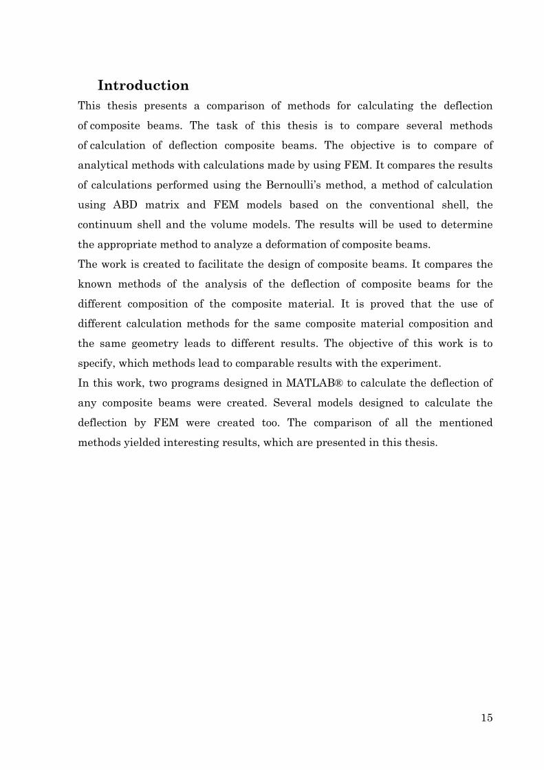
Introduction

This thesis presents a comparison of methods for calculating the deflection

of composite beams. The task of this thesis is to compare several methods

of calculation of deflection composite beams. The objective is to compare of

analytical methods with calculations made by using FEM. It compares the results

of calculations performed using the Bernoulli’s method, a method of calculation

using ABD matrix and FEM models based on the conventional shell, the

continuum shell and the volume models. The results will be used to determine

the appropriate method to analyze a deformation of composite beams.

The work is created to facilitate the design of composite beams. It compares the

known methods of the analysis of the deflection of composite beams for the

different composition of the composite material. It is proved that the use of

different calculation methods for the same composite material composition and

the same geometry leads to different results. The objective of this work is to

specify, which methods lead to comparable results with the experiment.

In this work, two programs designed in MATLAB® to calculate the deflection of

any composite beams were created. Several models designed to calculate the

deflection by FEM were created too. The comparison of all the mentioned

methods yielded interesting results, which are presented in this thesis.

16

1 Mathematical Description of Fibre Composite Material

1.1 Description of Anisotropic Material

For anisotropic material, with general anisotropy (there is not a single plane of

symmetry of elastic properties), both the stiffness matrix and the compliance

matrix has 21 independent elements. Matrices are based on Hooke’s law.

[1],[6] In system the Hooke’s law is expressed as follows

(1.1)

where is a symmetric matrix. The formula can be rewritten as

(1.2)

The equation can be expressed also in the inverse form

(1.3)

Matrix is also symmetric and it has a form

(1.4)

From comparison of relations (1.2) and (1.3) follows

(1.5)

But this work will deal mainly with orthotropic or transversely isotropic

materials; in those cases the numbers of independent variables are significantly

reduced.

1.1.1 Orthotropic Material

Orthotropic material has three mutually perpendicular planes of symmetry of

elastic properties. The stiffness matrix (and also the compliance matrix ) of

orthotropic material contains only 9 independent elements.

17

(1.6)

When elastic modules are used and substituted to the compliance matrix , we

obtain the relation

(1.7)

(1.8)

where are modules of elasticity in the main directions of anisotropy;

are shear modules in the planes parallel with the respective plane of

symmetry of the elastic properties ;

are Poisson’s ratio, where the first index corresponds to the direction

of the normal stress and the second direction which results in a corresponding

deformation in the transverse direction.

Because the matrix S and C are symmetric matrices, these are the equalities

between certain elements of the matrix

(1.9)

From Hooke’s law it is clear, that components of normal deformations are

dependent only on components of normal stress and shear deformations are

dependent only on shear components of stress. In this material, therefore, these

shear and normal components are not tied. [6]

18

Figure 1.1: Orthotropic material [1]

1.1.2 Transversely Isotropic Material

It is a material, which has a plane of symmetry of the elastic properties. This

plane is the same as a plane of isotropy, because the elastic properties in this

plane in all directions are the same. [1] If we substitute material constants into

compliance matrix , we get

(1.10)

Whereas the

is the modulus of elasticity in a direction perpendicular to the plane of

isotropy;

are modules of elasticity in the plane of isotropy;

are shear modules in direction perpendicular to the plane of isotropy;

are shear modules in the plane of isotropy;

are Poisson’s ratios expressing the ratio shortening (elongation) in the

plane of isotropy to elongation (shortening) in the main direction of anisotropy;

are Poisson’s ratios in the plane of isotropy;

the matrix can be written in a form

19

(1.11)

From the notation of matrix it is obvious that this matrix has only five

independent elements ( ), therefore the number of independent

material constants is also five ( ). [1]

From the Hooke’s law implies that the transversely isotropic material has no

relation between the normal and shear components of stress and strain. [1]

Figure 1.3: Schematic of deformation [5]

Figure 1.2: Transversely isotropic material [1]

20

1.2 Modules of Elasticity

1.2.1 Longitudinal Modulus

Figure 1.4: RVE subject to longitudinal uniform strain [4]

The assumption of the mathematical description of the composite material is that

the two materials are bonded together. More concretely: matrix and fiber

have the same longitudinal strain value noted . The main assumption in this

formulation is that the strains in the direction of fibers are the same in the

matrix and the fiber. This implies that the fiber-matrix bond is perfect. When the

material is stretched along the fiber direction, the matrix and the fibers will

elongate the same way as it is shown in the figure 1.4. This basic assumption is

needed to be able to replace the heterogeneous material in the representative

volume element (RVE) by a homogenous one. [4] The following derivation is

based on this assumption.

By the definition of strains according to the figure 1.4

(1.12)

Both fiber and matrix are isotropic and elastic, the Hooke’s law has a form for

fibre

(1.13)

and for matrix

(1.14)

21

The stress can be expressed as the loading force divided by the area where it

acts

(1.15)

So the average stress in the composite material acts in the entire cross section

of the RVE with area

(1.16)

where is the area of the cross section of the fibre and is the area of the

cross section of the matrix.

The applied total load is

(1.17)

Then

(1.18)

where

(1.19)

For the equivalent homogeneous material the stress is expressed as

(1.20)

Then, comparing (1.18) with (1.20), it gives the result

(1.21)

In the most cases, the modulus of the fibers is much larger than the modulus of

the matrix, so the contribution of the matrix to the composite longitudinal

modulus is negligible. This indicates that the longitudinal modulus is a fiber-

dominated property.

22

1.2.2 Transverse Modulus

Figure 1.5: RVE subject to transverse uniform stress [4]

In the determination of the modulus in the direction transverse to the fibers, the

main assumption is that the stress is the same in the fiber and the matrix. This

assumption is needed to maintain equilibrium in the transverse direction. Once

again, the assumption implies that the fiber-matrix bond is perfect. [4] The

loaded RVE is in the figure 1.5.

The cylindrical fiber has been replaced by a rectangular one (fig. 1.5), this is for

simplicity. Even micromechanics formulations do not represent the actual

geometry of the fiber at all. Both the matrix and the fiber are assumed to be

isotropic materials.

According to the situation in the figure 1.5, the stress in the matrix and in the

fiber is the same

(1.22)

so the strain is according to the Hooke’s law for the fiber

(1.23)

and for the matrix

(1.24)

These strains act over a portion of RVE; over , and over , while the

average strain acts over the entire width . [4] The total elongation is

(1.25)

23

Cancelling and again using Hooke’s law for the constituents the relation is

obtained

(1.26)

Using the equation (1.22) it is obtained the relation for the transversal

modulus

(1.27)

It is evident from the figure 1.5 that the fibers do not contribute appreciably to

the stiffness in the transverse direction, therefore it is said that is a matrix-

dominated property. This is a simple equation and it can be used for qualitative

evaluation of different candidate materials but not for design calculations. [4]

1.3 Stress and Deformation of Composite Material

Fiber reinforced composite is one of the most frequently used composite

materials. Great use is mainly due to the variability of this material. The

laminates usually consist of several layers of one-dimensional composite, wherein

each layer is composed of fibers and matrix.

Stiffness of unidirectional composites is expressed by the same relationships,

which are used for conventional materials (e.g. steel). The number of material

constants is only increased. From the point of view of micromechanics it is

possible to monitor tension only in the fiber or in the matrix. In this case, we

compute in terms of macromechanics so we will consider tension across the whole

layer of the laminate. This is called an intermediate stress in the layer.

Figure 1.6: An example of the unidirectional composite material [1]

24

Such a composite material can be regarded as the orthotropic respectively

transversely isotropic material. One-dimensional composite is represented in the

coordinate system . Fibres are oriented in the direction of the axis .

The axis is perpendicular to the fibres. Often the coordinate system

is often used, where means the longitudinal direction, is the transverse

direction and is the direction perpendicular to the lamina plane. Because the

thickness of one lamina is much smaller than its width and length, it is possible

to express the dependence between the stress and the deformation as in the case

of the plane stress. This greatly simplifies the task and the results are close to

reality. [1],[6]

Figure 1.7: An example of the unidirectional composite in the coordinate system [1]

The relation between stress and deformation is derived from assuming that the

lamina is a linearly elastic material. Consider orthotropic lamina is loaded by

tension in the fiber direction. Deformations are

(1.28)

where is the longitudinal tensile modulus and is a Poisson’s ratio defined

here.

In case of transversal tension the expressions are similar

(1.29)

where is the transversal tensile modulus and is the transversal Poisson’s

ratio.

For shear deformation we have

(1.30)

25

where is shear modulus in the plane .

The superposition principle can be used. Then the stress components have the

form

(1.31)

Component of deformation in the direction is for the case of the plane stress

(1.32)

where are transversal Poisson’s ratios.

The above relations can be summarized into a matrix equation

(1.33)

The compliance matrix for orthotropic material then has a form

(1.34)

Because the matrix is symmetric, the following relations hold.

(1.35)

As it is written in the introduction to this chapter, this is a case of the plane

stress. The tension vector has only three non-zero components. Expression (1.33)

can be rewritten as

(1.36)

For the inverse of equation (1.36) one writes

(1.37)

26

where

(1.38)

The elements specified stiffness matrix can be expressed by material constants

and . From these expressions it follows that for computation of

stress only four independent constants are needed.

(1.39)

The specific property of unidirectional composites is their change of strength and

stiffness depending on the direction in the plane . It is necessary to transform

stiffness quantities in different directions.

Figure 1.8: Unidirectional composite material in the two coordinate systems [1]

Figure 1.8 shows the unidirectional composite and two coordinate systems. The

system is rotated with respect to the system by an angle

around the axis . The formula for calculation of stress in the system

is

(1.40)

where is a transformation matrix for the stress vector and is the stress

vector in the coordinate system .

In 2D case the equation can be expressed in the form

27

(1.41)

A similar relation of course is applied for the transformation of strain

(1.42)

where is the transformation matrix for the strain vector. In components we get

(1.43)

In the previous paragraph it has been shown that the magnitude of stress and

strain are dependent on the direction in which they are examined. It is seen that

the stiffness matrix and the compliance matrix are not only dependent on

materials constants, but also on the position of the selected coordinate system.

We are looking for formulas of the stiffness matrix and the compliance matrix for

system , which is rotated relatively to the system by an

angle – . This is illustrated in the figure 1.8. The stiffness matrix and the

compliance matrix in the system are given by relations

(1.44)

(1.45)

The Hooke’s law for this rotated system can be expressed in a matrix form

(1.46)

Similarly, it is possible to form the relation for the deformation

(1.47)

The assumption that the width and length of the laminates are considerably

greater than its thickness is still valid. In this case it is still possible to consider

the plane stress. The three components of the stress can be expressed using the

three components of the deformation. For example, for the first component of the

tension vector the following relation is valid

28

(1.48)

In analogy the both the stress component and are obtained. These

relations can be written in the matrix form

(1.49)

For reduced stiffness matrix elements the following holds

(1.50)

By comparing the equations (1.37) and (1.49) the difference between the stiffness

matrix and the reduced stiffness matrix is apparent. The matrix has

generally all elements nonzero. That is, in Hooke's law (1.49) for off-axis

components of stress and deformation, the normal components of stress (with

indices ) are dependent also on the shear component (index ), inverse is

also true.

1.3.1 The Theory of the Laminate Deflection

Figure 1.9: A part of laminate in the plane [1]

In the figure 1.9 there is a part of the laminate in the plane . The side ,

which is in undeformed condition straight and perpendicular to the middle

surface of the laminate, remains even after deformation straight and

perpendicular to the middle surface. Due to the deformation arising at mid-plane

at point displacements are corresponding to the directions of axes

29

. Taking the derivatives of displacements we get the deformation field. This

can be written in the matrix form

(1.51)

where the deformation of midplane and the curvature stands for

(1.52)

Tension in k-th layer of the laminate can be expressed by equation for off-axis

strained layer of composite (1.49)

(1.53)

where is a reduced stiffness matrix.

Using equations (1.51) and (1.53) we obtain an expression for tension in the k-th

layer of the laminate

(1.54)

Since the tension in the laminate thickness varies discontinuously, resulting

forces and moments acting in cross-laminate are to be solved as a sum of the

effects of all the layers. For forces it is therefore possible to write

(1.55)

and for the moments

(1.56)

In these relations (1.55) and (1.56) the resultants of the forces have a

dimension [ ] i.e. the force per unit length and have a

dimension [ ] i.e. the moment per unit length, because these are resultant forces

and moments acting on the cross section of the k-th layer of the composite

material. [1]

30

On the basis of these relations a constitutive relation of the dependence of forces

and moments on deformations and curvatures can be formulated. Substituting

equations (1.55) and (1.56) into the equation (1.54) and using the expressions for

the deformation of the middle surface and the curvature of the plate (1.52). The

following equations are obtained

(1.57)

(1.58)

It is obvious that multiplying the integral with elements of the reduced stiffness

matrix of the individual laminas and integrating over the entire thickness of

the composite we obtain following expressions

(1.59)

(1.60)

where elements of the individual matrices are determined by relations

(1.61)

These relations can be expressed in a single equation

(1.62)

or

31

(1.63)

where is the extensional stiffness matrix, is the bending-extension coupling

stiffness matrix and is the bending stiffness matrix.

Constitutive equation of the laminate plate expresses forces and moments

depending on the curvature and on the mid-plane deformations. This matrix is

called the global stiffness matrix. For its notation, it is obvious that the matrix

binds force components in the median plane. The bending-extension coupling

stiffness matrix binds moment components and components of deformation in

the mid-plane and also components of vector of internal forces with components

of the curvature of the plate. matrix expresses the relation between the

components of moments and the curvature. This means that normal and shear

forces acting in the median plane not only cause the strain in the median plane,

but also the bending and the twisting of the middle area. Also components of the

bending moment cause strain in the median plane. [1],[4]

The relation (1.63) is used to calculate forces and moments in the laminate. In

practice most often stress and strain caused by external load are determined. A

form, which we want to achieve, is actually the inverse equation

(1.64)

where

(1.65)

Matrices and are called tensile, coupling and bending compliance

matrices. [1]

Ties between bend and tension or torsion and tension, and also between the

normal forces of the middle layer of the laminate and shear deformations are not

desirable in most cases. This phenomenon should be avoided during the

production of laminate’s appropriate order orientation of the layers.

32

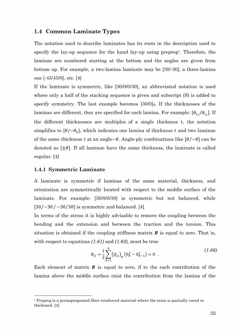
1.4 Common Laminate Types

The notation used to describe laminates has its roots in the description used to

specify the lay-up sequence for the hand lay-up using prepreg1. Therefore, the

laminae are numbered starting at the bottom and the angles are given from

bottom up. For example, a two-lamina laminate may be [30/-30], a three-lamina

one [-45/45/0], etc. [4]

If the laminate is symmetric, like [30/0/0/30], an abbreviated notation is used

where only a half of the stacking sequence is given and subscript (S) is added to

specify symmetry. The last example becomes [30/0]S. If the thicknesses of the

laminae are different, they are specified for each lamina. For example: [

. If

the different thicknesses are multiples of a single thickness , the notation

simplifies to [ , which indicates one lamina of thickness and two laminae

of the same thickness at an angle . Angle-ply combinations like can be

denoted as . If all laminae have the same thickness, the laminate is called

regular. [4]

1.4.1 Symmetric Laminate

A laminate is symmetric if laminae of the same material, thickness, and

orientation are symmetrically located with respect to the middle surface of the

laminate. For example: [30/0/0/30] is symmetric but not balanced, while

is symmetric and balanced. [4]

In terms of the stress it is highly advisable to remove the coupling between the

bending and the extension and between the traction and the torsion. This

situation is obtained if the coupling stiffness matrix is equal to zero. That is,

with respect to equations (1.61) and (1.62), must be true

(1.66)

Each element of matrix is equal to zero, if to the each contribution of the

lamina above the middle surface exist the contribution from the lamina of the

1 Prepreg is a preimpregnated fiber-reinforced material where the resin is partially cured or

thickened. [4]

33

same properties and orientation in the same distance below the middle surface

(see figure 1.10).

Figure 1.10: Symmetric laminate [1]

It must be true

(1.67)

If each layer above the middle surface will correspond to the identical layer under

the middle surface, it is the symmetrical laminate. The global stiffness matrix

from equation (1.63) will be in the form

(1.68)

A binding between tensions and the bending, which constitutes the matrix is a

result of a sequence of the layers. It does not follow from the anisotropy or the

orthotropic layers. It is the result of a sequence of layers. This relation also exists

in the composites made of two different metal isotropic materials (bimetal). Due

to changes in temperature the bending of the composite is visible.

1.4.2 Antisymmetric Laminate

An antisymmetric laminate consists of an even number of layers (see figure 1.11).

It has a pairs of laminae of opposite orientation but of the same material and

thickness symmetrically located with respect to the middle surface of the

laminate. For example: [30/-30/30/-30] is an antisymmetric angle-ply laminate

and [0/90/0/90] is an antisymmetric cross-ply. [4]

34

Therefore, for each two plies of the same material properties is true

(1.69)

From this two conditions follows that both plies have the same thicknesses and

they are at the same distance from the middle surface.

Figure 1.11: Antisymmetric laminate [1]

The global stiffness matrix from equation (1.63) of the antisymmetric laminates

has a form

(1.70)

Antisymmetric laminates have elements equal to zero

(1.71)

but they are not particularly useful nor they are easier to analyze than general

laminates because the bending extension coefficients and are

not zero for these laminates. [4]

1.4.3 Quasi-isotropic Laminate

Quasi-isotropic laminates are constructed to create a composite, which behaves

as an isotropic material. The in-plane behaviour of quasi-isotropic laminates is

similar to that of isotropic plates but the bending behaviour of quasi-isotropic

laminates is quite different than the bending behaviour of isotropic plates. [4]

In a quasi-isotropic laminate, each lamina has an orientation given by

35

(1.72)

where is the lamina number, is the number of laminae (at least three), and

is an arbitrary indicial angle. The laminate can be ordered in any order like

[ ] or [ ] and the laminate is still quasi-isotropic.

Quasi-isotropic laminates are not symmetric, but they can be made symmetric by

doubling the number of laminae in a mirror (symmetric) fashion. For e.g. the

[ ] can be made into a [ ], which is still quasi-

isotropic. The advantage of the symmetric quasi-isotropic laminates is that they

have the coupling stiffness matrix . [4]

The tensile stiffness matrix and the bending stiffness matrix of isotropic

plates can be written in terms of the thickness of the plate and only two

material properties, the modulus of elasticity and the Poisson’s ratio as

(1.73)

and

(1.74)

Quasi-isotropic laminates have, like isotropic plates, , but they have

and , which makes quasi-isotropic laminates quite

different from the isotropic materials as it is seen below

(1.75)

and

(1.76)

Therefore, formulas for the bending, the buckling and vibrations of isotropic

plates can be used for quasi-isotropic laminates only as an approximation. The

formulas for isotropic plates provide a reasonable approximation only if the

laminate is designed trying to approach the characteristics of isotropic plates

36

with and . This can be achieved for symmetric quasi-

isotropic laminates, which are balanced and have a large number of plies.

37

2 The Theory of the Deflection

The deflection is a kind of stress, in which a straight beam is curved to a plane or

a three-dimensional curve. The beam is called a straight rod that it is loaded

mainly to the bending. The beam bending is one of the most common types of

stresses at all (e.g. all shafts are beams). The properties of the beam are

substantially dependent on the type of its support. [2]

This work deals with the encastre composite beams loaded by concentrated

force at the end of its length. (Figure2.8) The bending of the beam will be solved

by determination of the deformation energy due to the bending moment and the

shear force. The deformation of the beam is determined using Bernoulli’s method.

Every cross-section of the bended beam transfers the bending moment and

the shear force . The shear forces and the bending moments are caused by one

common cause, namely the external loading. A relation between them is shown in

the figure 2.1.

Figure 2.1: Loaded beam and out of joint element with force effects [2]

In the right side of the figure 2.1 there is an element of the beam with the force

effects acting on it. The element of the beam has to be in equilibrium. The

equilibrium equations of this element are known as the Schwedler theorem. [2]

For the shear force we have

(2.1)

and for the bending moment

(2.2)

38

As a result of those effects of the shear force and the bending moment there

is some tension. For simplicity, one considers only the case of load by bending

momentum. This case is called a pure bending. For a pure bending is proved the

validity of the Bernoulli hypothesis. This hypothesis says that the planar cuts,

which were perpendicular to the longitudinal axis of the beam before the

deformation, remain plane after deformation and are perpendicular to the

deformed longitudinal axis of the beam. [2] This is shown in the figure 2.2 and

1.9.

Figure 2.2: Deformation of the beam according the Bernoulli hypothesis [2]

From the figure 2.2 it is evident that an elongation and a relative elongation

of the beam

(2.3)

39

are proportional to the distance from the neutral axis . As the Hooke’s law is

valid

(2.4)

one can express as

2

(2.5)

where is stress, is the bending moment, is the moment of inertia to the

axis and is the distance from the neutral axis to the top or the bottom of

the section, as it is shown in the figure 2.2.

If one substitutes the relation (2.5) to the Hooke’s law (2.4), one gets

(2.6)

where is the relative elongation in a direction of the -axis.

The important characteristic of the deformation curve of the beam is its

curvature . From the figure 2.3 one can express the elongation as

(2.7)

The curvature of the beam is possible to express as

2 The whole derivation is in the literature [2].

Figure 2.3: The part of the beam with marked extension [2]

40

(2.8)

From the equation (2.8) one derivates the differential equation of the deflection

line, if one substitutes the known relation of the analytical geometry, which

express the curvature of the planar curve , to the equation of the curvature

of the beam.

(2.9)

To the deflection referred in the figure 2.3 corresponds the sign minus

( ). For the small values one can neglect the term . So the

simplified relation is obtained

(2.10)

The differential equation of the elastic deflection line

(2.11)

presented the Swiss mathematician J. Bernoulli in 1694. [2]

2.1 The Moment of Inertia

If the coordinate system is defined as in the figure 2.4, the cross section lies in

the plane .

Figure 2.4: The beam placed in coordinate system and the plane of the cross section [2]

According to the figure 2.4 one removes the element from the cross

section which has the coordinates and relative to the axes and . [2]

41

The moment of inertia to the axis is expressed by the relation

(2.12)

Analogically the moment of inertia to the axis can be defined

(2.13)

For the beams with a circular cross section it is appropriate to establish the polar

coordinates as it is shown in the figure 2.5.

Figure 2.5: The cross section of the circular beam with the cylindrical coordinates [2]

Generally the relation

(2.14)

is valid.

To solve the moment of inertia on the wound fibreglass pipe the additivity of the

moment of inertia is utilized. The moment of the whole pipe is computed as a

sum of the moments of individual layers

(2.15)

where is the external diameter of the each layer, is the internal diameter of

the each layer and is the number of layers.

We will use this property to computation of the bending stiffness in chapter 3.

42

2.2 The Determination of the Deformation Energy

2.2.1 The Deformation Energy from the Pure Bending

The pure bending is the uniaxial stress; therefore, the derivation of the

deformation energy is based on the equation for density of the deformation

energy

(2.16)

The magnitude of the stress is a function of a position. The relation is based on

the form of the element (figure 2.6), where the stress is regarded as a constant.

The energy of this element is determined, and then the value of the deformation

energy in the entire beam by integration is determined. [2], [6]

Figure 2.6: Cross section of the general beam [2]

The selected element has a volume

(2.17)

where is an element of the area and is an element of the distance in the

direction of - axis. In this element the energy is accumulated

(2.18)

For the bending stress the relation is valid

(2.19)

After the substitution of the equation (2.19) to the (2.18) one gets

43

(2.20)

The total energy accumulated in the beam one can express by the integration

with respect to and

(2.21)

after editing

(2.22)

Because the relation for the moment of inertia is valid

(2.23)

the relation for the deformation energy of the beam is

(2.24)

In case, that the relation - the beam has a constant cross-section,

one can write

(2.25)

2.2.2 The Deformation Energy by the Shear Force

In case of the deformation energy caused by the shear stress the relation is

generally valid

(2.26)

where is an elementary deformation energy, is a shear modulus and is

an elementary volume. [2]

The shear stress from the shear force depends on the shape of the cross-section.

The determination of the expression of the energy from the shear force we

perform on the beam with the rectangular cross-section. In this case it is valid

the expression

44

(2.27)

and

(2.28)

where is the shear force according to the Schwedler’s theorem (2.1), is the

moment of inertia with respect to the neutral axis is a static moment of the

area (

), is magnitude of shear stress which should be created

if it was spread evenly over the entire cross-section and is the width of the

rectangular cross-section; if one used the designation from the figure 2.7.

Figure 2.7: The cross section of the rectangular beam loaded with shear [2]

If the beam has a length , then the following relation is valid

(2.29)

and after substitution

(2.30)

Because the centre shear stress is the deformation energy is

(2.31)

After integration and editing one obtains

45

(2.32)

As it is apparent from the expression of the deformation energy from the

influence of the shear force, at the beam with a rectangular cross-section due to

the nonlinear distribution of shear stresses the coefficient has been added. The

same result one obtains for beams with other shapes of the cross-section, but

with another coefficient . [2] The general relation for the deformation energy

from shear force is

(2.33)

The coefficient depends on the shape of the cross-section

(2.34)

For the rectangular cross-section we obtain

, for circular cross-section is

and for eg. I-beams is . [2]

2.3 The Deflection of the Beam

The deflection of a composite beam has two components, bending and shear

(2.35)

where is the total deflection, is the bending deflection and is the shear

deflection. The bending deflection is controlled by the bending stiffness ( )

and the shear deflection by the shear stiffness ( ). [4]

Shear deformations are neglected for metallic beams because the shear modulus

is high ( ), but shear deformations are important for composites because

Figure 2.8: The model of the beam used for analysis

46

the shear modulus is low (about or less). The significance of the shear

deflection with respect to the bending deflection varies with the span, the

larger the span the lesser the influence of the shear (compared to bending). [4]

Calculation of the beam bending is made to a cantilever beam (figure 2.8), which

is used for the analysis of the following methods for calculating the deflection.

First, we determine the diagram of the shear force and the diagram of the

bending moment . It is illustrated in the figure 2.9.

Figure 2.9: The loaded beam with the course of shear force


(2.36)

The deformation energy is determined as a sum of the bending deformation

energy and the shear deformation energy. The equation (2.25) and (2.33) is used.

(2.37)

Because the cross section of the beam is constant, the moment of inertia is

constant too, so we can factor them out. For the respective deformation energies

we have

(2.38)

and

(2.39)

The expression for the total energy is therefore

(2.40)

47

For the calculation of the deflection at the end of the beam under the force we

use the Castigliano’s theorem3

(2.41)

The same result we get if we use the Mohr’s Integral, which follows from the

Castigliano’s theorem.

(2.42)

(2.43)

The relation for the deflection at the end of the beam will have a form

(2.44)

1.

3 The detailed derivation of the Castigliano’s theorem can be found in the literature [2].

48

3 The Methods Used for the Analysis

3.1 The Used Model of the Beam

Figure 3.1: The model of the beam used for the analysis

All computations for the analysis of the composite beam bending are designed for

the cantilever beam that is loaded with concentrated force at the end of its

length. The beam is a wound composite pipe with a circular cross section. All

data used for computations are presented in the table 3.1 below.

3.2 The Calculation of the Beam Bending by Bernoulli’s

Method

For the calculation of the bending by this method the Castigliano’s method is

used, which is the same method as the calculation of the bending of the isotropic

material, with an extension for shear. The validity of the Bernoulli’s hypothesis is

still assumed as it is written in the previous chapter 2.

Input data

Geometry

length L = 1 m inner diameter d = [2, 4, 6, 8, 10] mm thickness of each composite

layer

t = 1 mm

thickness of the wound pipe tp = 3 mm Load

concentrated force F = 100 N Material

density ρ 7 kg m3 longitudinal modulus of

elasticity

EL = 156.05 GPa

transversal modulus of

elasticity

ET = 6.045 GPa

shear modules GLT = 4.431 GPa GLT’ = 4.431 GPa GTT’ = 4.431 GPa Poisson’s ratio νLT = 0.328 layup of composite material α -α angle of fiber α 7 Table 3.1: Input data used for analysis

49

(3.1)

The Castigliano’s method (3.1) is adjusted to the form (2.42) that is called Mohr’s

Integral.

(3.2)

Shear effects cannot be ignored, because in the bending of the composite beam it

has a larger share of the total bending than in the isotropic material.

The composite theory enters this computation in the calculation of the modulus of

elasticity . It is known, that the effect in each layer may be different so this

problem must be included in the computation. A modulus of elasticity of each

layer is calculated using the stiffness matrix in the main coordinate system

of the composite material.

(3.3)

, are tensile modules in the direction and ; and are Poisson’s

ratios; is a shear modulus; is index of each layer; is a number of layers.

The stiffness matrix must be transformed to the coordinate system of

the whole beam by the transformation matrix .

(3.4)

where is a rotation angle around the - axis. (Angle may be different for each

layer.)

Then, we can do the transformation.

(3.5)

To express the modulus of elasticity in main coordinate system the

compliance matrix is needed. The compliance matrix is the inverse matrix to

the stiffness matrix .

(3.6)

50

From this matrix we choose the following elements to determine the modulus of

elasticity and the shear modulus for each layer.

(3.7)

(3.8)

The resultant bending stiffness is obtained by adding the product of the

modulus of elasticity and an appropriate quadratic moment of the cross section

for each layer

(3.9)

(3.10)

where is the external diameter of each layer, is the internal diameter of each

layer, is the index of each layer and is the number of layers. To obtain the

resultant equivalent shear stiffness we proceed similarly

(3.11)

(3.12)

Again, is the external diameter of each layer, is the internal diameter of each

layer, is the index of a layer and is the number of layers.

The deflection is calculated from the equation (3.2). The determination of the

diagram of the shear force and the bending moment is the same in the

section 2.3

(3.13)

and the bending moment by a dummy force is

(3.14)

as it is illustrated in the figure 3.2.

51

Figure 3.2: The beam loaded by the unit force with the course of the shear force


Then, the Mohr’s integral is computed according to the equation (2.42)

(3.15)

After the integration that is

(3.16)

where is the force load, is the length of the beam, is the distance on the

-axis, is the coefficient characterizing the unequal distribution of the shear

stress. The coefficient depends on the geometry of the cross section

(section 2.2.2) and is the sectional area of the beam.

After substituting we obtain the deflection in the place under the force .

(3.17)

This computation of the bending is based on the compliance matrix . The

resultant deflection thus represents the upper limit of the safety. The deflection

provides greater or equal values in the comparison with other methods of the

deflection. If we use the stiffness matrix for the calculation of the deflection, we

will obtain another limit value, this time the lower limit of the beam deflection.

These values correspond to the application of the longitudinal modulus of

elasticity (the lower value of the deflection) and transversal modulus of elasticity

(the upper value of the deflection) to the computation of bending. This fully

agrees with the theory of composite materials.

For this method of the computation bending a program DP_Trubka.m in

MATLAB® was created. Program calculates the bending of the beam of the

52

circular cross section for any number of layers. The structure of composite

material may also be arbitrary. With this program the data to the summary

graphs (4.1-5) of the dependence of the bending of a beam on the angle of the

direction of the fibres in the composite material have been calculated. The overall

listing of the program is presented in Annex [1.1].

3.3 The Calculation of the Bending of the Composite Beam

Using ABD Matrices

For the calculation of the beam bending with a circular cross section (figure 3.1)

by this method the equation (1.63)

described in the chapter 1 is used.

First, we determine all input values. These are geometrical dimensions and

material constants for all layers described in the table 3.1 in the section 3.1.

Then, we can put together the stiffness matrix in the principal coordinate system

(3.19)

Its elements are determined by these relations (1.39) in the section 1.3

(3.20)

The transformation into the global coordinate system of the beam is necessary.

This is realized according to the formula (1.44)

(3.21)

In a completely general case one needs a reduced stiffness matrix to compute,

but this is a planar case, so the off-axis stiffness matrix is equal to the stiffness

matrix transformed to the global coordinate system.

(3.18)

53

(3.22)

Now we can compute the elements of stiffness matrices , and according

to the formulas (1.61)

(3.23)

In our case we use the matrix to compute the equivalent modulus of elasticity

of our beam. The strain is planar and the matrix is zero so the equation has

a form

(3.24)

Then we can divide the matrix notation to the two equations

(3.25)

and

(3.26)

From the second equation (3.25) we obtain a relation of deformation to the middle

area in directions and

(3.27)

This relation we substitute to the first equation (3.24)

(3.28)

As it is written in the section 1.3 the resultant of the force has a dimension

[ ], so this is not an expression of a stress. The stress of the composite

material we can express using the Hooke’s law (2.4). To obtain an expression of

the stress from this relation (3.28), it is necessary to divide the entire expression

by the total thickness of the composite material. From the relation (3.28) it is

evident, that the modulus of elasticity corresponds to the expression in brackets

divided by the total thickness of the laminate .

54

(3.29)

The equivalent modulus of elasticity for this case one can express by the

formula

(3.30)

where are the elements of the extensional stiffness matrix and is the

thickness of the composite material.

The equivalent shear modulus is obtained the same way from the equation

(3.18). The assumptions are similar as in the previous case. The matrix is zero

and the pure shear stress is considered. The equation has a form

(3.31)

Again we can divide the matrix notation to the two equations

(3.32)

and

(3.33)

From the first equation (3.32) we obtain a relation of the deformation to the

middle area in directions and

(3.34)

This relation we substitute to the second equation (3.33)

(3.35)

Once again the shear force has a dimension [ ], so this is not an

expression of the shear stress. The shear loading we can express using the

generalized Hooke’s law

(3.36)

To obtain an expression of the shear from the relation (3.18), the entire

expression (3.35) is necessary to divide by the total thickness of the composite

material. From this relation (3.35) it is evident, that the shear modulus

corresponds to the expression in brackets divided by the total thickness of

laminate .

55

(3.37)

The equivalent shear modulus for this case one can express by the formula

(3.38)

where are elements of the extensional stiffness matrix and is the thickness

of composite material.

The following is a substitution of and into the formula for the calculation

of bending (2.44), which is

(3.39)

This method is only approximate, because it includes several inaccuracies. First,

to calculate modulus of elasticity we assume the plane stress and the pure shear.

We count with the unwound circular cross-section of the beam. Second, we

assume that the bending-extension coupling stiffness matrix is zero. This

precondition is fulfilled only for specific compositions of the composite material as

is the symmetric laminate (section 1.4.1). This greatly reduces the possibility of

either using the method or we will admit the neglect of certain bonds in the

material. [1] Although this method is approximate, it shows that it gives

significant results. These assumptions do not bring a considerable mistake into

the calculation.

For this method of the computation of the bending a program

DP_ABD_Trubka.m in MATLAB® was created. (Annex [1.2]) The program

calculates the beam bending of the circular cross section for any number of

layers. The structure of the composite material may also be arbitrary. The output

data are summarized into graphs of the dependence of the beam deflection on the

angle of the direction of the fibres in the composite material.

3.4 The Calculation of the Beam Bending by the Finite

Elements Method

In this work all FEM models are created with Abaqus CAE. There are three

options that can be used for the modelling of the composite beam by the finite

elements method:

56

conventional shell

continuum shell

volume model

The specifics of each method are presented in the following sections. This is not a

tutorial to get started with the modelling in Abaqus, but there are captured

substantial differences of individual models and there are information to

reconstruct the models of the composite beam.

For each model was created a CAE file, where was specified geometry, materials,

loads and constraints. Then, it was generated a script in Python (the

programming language for Abaqus) of this CAE file. In this script variables were

edited (the cross-sectional size and the angle of the direction of the fibres) to

obtain particular data for each combination of the diameter and the angle of

fibres. The script is shown in Annexes [1.3-5]. Values of calculated deflections are

shown in table 4.1. For every model the same input data have been used. This is

written in the table 3.1.

3.4.1 The Calculation by Using Conventional shell

The whole geometry is represented at a reference surface. The reference surface

of the shell is defined by the shell element’s nodes and normal direction.

Thickness is defined by section property. The input data was chosen according

the table 3.1. The following is a description of the operations in Abaqus CAE to

obtain a script in Python.

The following is a description of the operations in the particular modules of CAE:

Sketch

For the modelling of the geometry of the pipe as a conventional shell one used the

Part manager →Create Part →Shell, Extrusion. Then, a sketch is made as is

shown in the figure 3.3.

57

Figure 3.3: The sketch for the model of the pipe

Property

The material has to be determined. One used the Material manager → Create

and set the density of the chosen material ant its constants. For the modelling of

a composite material the type Lamina is used. The details are shown in a figure

(3.4) below. In Abaqus we have to specify the shear modules in all three

dimensions. For our task was chosen the same value in all dimensions as it is

written in the table of input values (3.1).

Figure 3.4: The window for editing the material

When the material is determined, the composite layup can be defined using

Composite Layup Manager → Create →Conventional Shell. One sets the

58

coordinate system for the used geometry, the normal direction, the number of

plies and their properties. The thickness of plies, the material, the rotation angle

and the coordinate system for all plies are specified (figure 3.5). There is also

specified the geometry area for each ply.

Assembly

If the properties of material and geometry are determined one can set the

assembly. In this case the assembly contains one part – the shell of the pipe. As

we can see in the figure (3.6) the assembly includes two coordinate systems. It is

caused by our specification of the coordinate system for the direction of fibers.

The coordinate system, which is used for the computation, has the x-axis

identical to the longitudinal axis of the pipe (in the figure (3.6) it is on the left

side). The second one is automatically generated for the assembly (it is on the

right side in the figure (3.6)).

Figure 3.5: The window for editing the composite layup

Now the partition of the shell into two parts is made. It is for the better

identification of the direction of the composite material and also for the better

meshing of a part. The partition is made by the order Partition Cell: Use

Datum Plane. First one has to create the datum plane by using the order

Create Datum Plane: 3 Points.

59

Step

In the mode Step the procedure type Static, General is defined, because we are

computing the static case of the beam bending. The point of our interest is a size

of the bending at the end of the beam, so the only calculation of the translation is

needed. This we specify in the Field Output Request Manager → Cerate →

Continue → Edit Field Output Request, where we choose the possibilities as it

is shown in the figure (3.7 b).

a) b)

Figure 3.7: a) The window to specify the calculating step

b) The window for choosing the outputs

Interaction

The beam is loaded by a concentrated force, therefore it is appropriate to place

the force into the centre of the circular cross-section at the end of the beam. The

Figure 3.6: The assembly of the beam

60

centre of the cross-section has to be connected with a cross-section at the end of

the beam. This we can define by the Constraint Manager → Create →

Coupling →Edit Constraint. Before that we determine the reference point

(RP-1 in the figure (3.8 a)) for a coupling by the order Create Reference Point

in the centre of the cross-section at the end of the beam.

a)

b)

Figure 3.8: a) The pipe with the shown coupling properties


Than we set a coordinate system for the coupling, we choose the same one we

have used for the determination of the composite material specification (the red

one in the figure (3.8 a)).

Load

In this module the size of the concentrated force and its location is specified as

well as fixation of the beam. The concentrated force is defined in Load Manager

→ Create → Concentrated Force → Edit Load. We define a coordinate system

that we used (the red one in the figure (3.9 b) and a force in the direction of the

-axis as it is shown in the figure (3.9 a).

The fixation of the beam is specified in Boundary Condition Manager →

Create → Symmetry/Antisymmetry/Encastre → Encastre (

). Again the coordinate system has to be defined.

61

a)

b)

Figure 3.9: a) The window for editing the load

b) The pipe with the shown load and the fixation

Figure 3.10: The window for editing the boundary conditions

Mesh

The element type S4R has been used for the meshing of the pipe. S4R is a robust,

general-purpose element that is suitable for a wide range of applications. The

size of elements has been chosen 0,005 x 0,001. It is not an optimal choice of a

size for this type of elements, because the aspect ratio should be less than three.

But we do not review some local effects on the geometry, for calculating the

deflection of the whole beam this selection of the size of elements does not distort

the calculation.

62

Figure 3.11: The meshed beam

Job

The calculation was carried out without errors. Details can be seen in the figure

(3.12).

Figure 3.12: The listing of the calculation

Visualization

The deformation of the beam was most reflected as it has been expected in the

direction of the concentrated force. It is evident from the figure (3.13 a).

63

a)

b)

Figure 3.13: a) The deformed beam shown in the plane

b) The deformed beam in a general perspective with the scale

The value of the deflection is different in individual nodes in the cross-section.

This is shown in the figure (3.14). So the numerical size of the bending was

calculated as the average of values of the deformation in the direction of the -

axis of individual nodes at the end of the beam.

Figure 3.14: The detail of the end of the deformed beam with the values of the deflection

64

3.4.2 The Calculation by Using the Continuum Shell

For the calculation using the continuum shell the full 3-D geometry is specified.

The element thickness is defined by the nodal geometry. Continuum shell

captures more accurately the through-thickness response for composite laminate

structures. It has a high aspect ratio between in-plane dimensions and the

thickness. The input data were chosen according the table 3.1. The following is a

description of the operations in Abaqus CAE to obtain a script in Python.


Sketch

For modelling the geometry of the pipe as a continuum shell one used the Part

manager → Create Part →Solid, Extrusion. Then a sketch is made by two

circles as it is shown in the figure (3.15).

Figure 3.15: The sketch for model of the pipe

Property

In the module Property the material has to be determined. One used the

Material manager → Create and set the density of the chosen material and its

constants. For the modelling of a composite material the type Lamina is used.

The details are shown in the figure (3.16) below. This part is the same as in the

section 3.4.1 (modelling of the conventional shell).

When the material is determined, the composite layup can be defined using

Composite Layup Manager → Create → Continuum Shell as it is shown in

the figure (3.17). One sets the coordinate system for the used geometry, the

normal direction, the number of plies and their properties. The thickness of plies,

the material, the rotation angle and the coordinate system for all plies are

specified. There is also specified the geometry area for properties of each ply. The

65

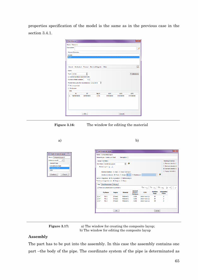
properties specification of the model is the same as in the previous case in the

section 3.4.1.


a) b)

Figure 3.17: a) The window for creating the composite layup;

b) The window for editing the composite layup

Assembly

The part has to be put into the assembly. In this case the assembly contains one

part –the body of the pipe. The coordinate system of the pipe is determinated as

66

we can see in the figure (3.18). It is the coordinate system, which is used for the

determination of the direction of fibres. The coordinate system that is used for

the computation has the -axis identical to the longitudinal axis of the pipe.


Now the partition of the geometry into two parts is made. It is for the better

identification of the direction of the composite material and also for the better

meshing of the part. The partition is made by order Partition Cell: Use Datum

Plane. First, one has to create the datum plane by using order Create Datum

Plane: 3 Points.

Figure 3.19: The window for choosing the outputs

67

Step

As it is written in the section 3.4.1, the procedure type Static, General is

defined. The outputs are set as in the previous case, where we choose the

possibilities of the displacement as is shown in the figure (3.19).

Interaction

Again the one end of the beam is prepared for the loading using Constraint

Manager → Create → Coupling →Edit Constraint. The reference point

(RP-1 in the figure (3.20 a)) is set. According to our model the beam is loaded by

a concentrated force, which is placed into the centre of the circular cross-section

at the end of the beam. The centre of the cross-section has to be connected with a

cross-section at the end of the beam by constraint. The coordinate system is

selected as in the previous case according to the specification of the composite

material.

Load

Further, the concentrated force and the fixation of the beam are determined. The

concentrated force is defined in Load Manager →Create →Concentrated

Force →Edit Load. We define a coordinate system that we have used before (the

red one in the figure (3.21 a)) and a concentrated force in the direction of the

-axis as it is shown in the figure (3.21 b).

a) b)



68

The support of the beam is specified in Boundary Condition Manager →

Create → Symmetry/Antisymmetry/Encastre → Encastre (

). The coordinate system has to be defined. The fixation is

accomplished in the same way as in the previous section 3.4.1.

Mesh

Continuum shell elements are 3-D stress/displacement elements for the use in

the modelling of structures that are generally slender, with a shell-like response

but the continuum element topology. They capture more accurately the through-

thickness response for composite laminate structures. The element type SC8R

(8-node hexahedron for a general purpose) has been used for the meshing the

geometry. The thickness direction can be ambiguous for the SC8R element. Any

of the 6-faces could be a bottom face, therefore it is important to define the

bottom side of the elements and assign the stack direction. This can be

determined by order Assign Stack Direction as it is shown in the figure (3.22).

The size of elements has been chosen 0,005m along the -axis and the quantity

40 elements along the perimeter.

a)

b)

Figure 3.21: a) The pipe with the shown load and the fixation


69

Figure 3.22: The meshed beam with the layup orientation

Job


(3.23).


Visualization

Deformation of the beam was most reflected as it has been expected in the


The value of the deflection is the same in individual nodes in the whole cross-

section. This is shown in the figure (3.25). So the numerical size of the deflection

was taken as the value of the deformation in one node at the end of the beam.

70

a)

b)




71

3.4.3 The Calculation Using the Volume Model

For the calculation using the volume model the full 3-D geometry is specified and

each ply is created separately as a separate body. The input data were chosen

according to the table 3.1 of the input data. The following is a description of the

operations in Abaqus CAE to obtain a script in Python.


Sketch

For modelling the geometry of a pipe as a volume model one used the Part

manager →Create Part →Solid, Extrusion as by the modelling of the

continuum shell. Then, a sketch is made by two circles for each ply as it is shown

in the figure (3.26).

Figure 3.26: The sketch of the one layer for model of the pipe

Property

In this module the material and its orientation has to be determined. One used

the Material manager → Create and set the density of a chosen material and

its constants. For modeling a composite material the type Engineering

Constants is used. Poisson’s ratio in all three dimensions has to be determined

as well as the module of elasticity and the shear module. Poison’s ratio was

defined the same in all directions

72

The modules of elasticity and in the direction of -axis and -axis were

defined equal as the transversal modulus of elasticity

The shear modules ware defined as in previous models of composite beams

according to the table of input values 3.1. The details are shown in the figure

(3.27) below.


When the material is determined, the composite layup can be defined. For

modelling the composite beam using the volume model each ply must be

determinated separately, because we have a part for each ply. The material of

each ply we determine using Section Manager → Create → Solid, Composite,

and then one can set the material of the ply, the rotation angle and the element

relative thickness as it is shown in the figure (3.28 a). This operation is repeated

with each layer.

The material orientation is defined by Assign Material Orientation. It is

important for the determination of the direction of fibres in the composite

material. The direction is defined with respect to the coordinate system that has

the -axis coincident with the longitudinal axis of the pipe (the purple one in the

figure (3.29)).

73

a)

b)

c)

Figure 3.28: a) The window for creating the composite type of section

b) The window for choosing the section for editing its properties

c) The window for editing the composite layup

Figure 3.29: The window for specify the orientation of the material

Assembly

Parts have to be put into the assembly. In this case the assembly contains three

parts – one part for each ply of the pipe. The coordinate system of the pipe is

determinated as we can see in the figure (3.30). It is the coordinate system, which

74

is used for the determination of the direction of fibres. Three parts are put

together to make a model of the wound composite pipe as one can see in the

figure (3.30).


Now the partition of the geometry into two parts of each ply is made. It is for

better identification of the direction of the composite material and also for the

better meshing of the parts. The partition is made by the order Partition Cell:

Use Datum Plane. First, one has to create the datum plane by using the order

Create Datum Plane: 3 Points.

Step

As it is written in previous sections 3.4.2, the procedure type Static, General is

defined. The outputs are set the same way as in the previous case, where we

choose the possibilities of displacement as it is shown in the figure (3.31).

Interaction

The end of the beam is prepared for the loading using Constraint Manager →

Create → Coupling → Edit Constraint. The reference point (RP-1 in the

figure (3.32 a)) is set in the centre of the cross section as it is made in previous

models. The coordinate system is selected according to the specification of the

composite material. In this case all three parts have to be connected with the

constraint as it is shown in the figure (3.32).

75

Figure 3.31: The window for choosing the outputs

a)

b)



Load

The concentrated force is defined in Load Manager → Create → Concentrated

Force → Edit Load. We define a coordinate system that we used before (the red

one in the figure (3.33 a)) and a concentrated force in the direction of the -axis.

This is shown in the figure (3.33 b).

76

a)

b)

Figure 3.33: a) The pipe with the shown load and the fixation


The support of the beam is once again specified in Boundary Condition

Manager → Create → Symmetry/Antisymmetry/Encastre → Encastre (

). The coordinate system has to be defined. The

fixation is accomplished in the same way as in previous sections, but there have

to be fixed all three parts. This is illustrated in the figure (3.34 a).

a)

b)

Figure 3.34: a) The beam with shown the fixation

b)The window for editing the boundary condition

Mesh

The element type C3D8R (three-dimensional hexahedral element) has been used

for meshing the pipe. These elements are linear, reduced-integration elements. A

good mesh of C3D8R elements usually provides a solution of accuracy at less cost.

Quadrilateral and brick elements are preferred when such meshing is

77

reasonable. The size of elements has been chosen 0,005m along the -axis,

quantity 40 elements along the perimeter as in the continuum shell model and

five elements across each layer. It is not an optimal choice of size for this type of

elements, because the aspect ratio should be less than three. But we do not

review some local effects on the geometry, for calculating the deflection of the

whole beam this selection of size of elements does not distort the calculation in

the general scale.

Figure 3.35: The meshed beam

Job


(3.36).


78

Visualization

Deformation of the beam was most reflected as it had been expected in the


The value of the deflection is different in individual nodes in the whole cross-

section. This is shown in the figure (3.38). So the numerical size of the bending

was calculated as the average of values of the deformation in the direction of the

-axis of individual nodes at the end of the beam.

a)

b)



79


80

4 Results

The beam bending has been calculated by methods mentioned in the previous

chapter. For all analyzed methods was used the same model of the beam and the

same properties of a material, which they are specified in the table of Input data

3.1. All obtained values of the deflection are listed in the table 4.1 below.

Table 4.1: The numerical results of the analysis of the methods for calculation the deflection

For both analytical methods (Bernoulli’s method and the method using ABD

matrix) the deflection was computed with the shear effect as it is written in the

Deflection (m)

d (mm) 0 5 15 25 35 45 55 65 75 85 90

2 1,13096 1,40923 3,53913 7,32757 12,00693 16,76582 20,95840 24,20021 26,34762 27,40277 27,53341

1,13048 1,40875 3,53867 7,32714 12,00653 16,76543 20,95800 24,19978 26,34716 27,40230 27,53293

3,25266 3,31299 3,69472 4,29963 5,10820 6,15034 7,51986 9,46172 12,94770 20,79490 22,20870

1,46525 1,51444 1,86764 2,65495 4,28955 7,44343 12,89239 20,64141 28,39480 32,72279 33,20780

1,14427 1,34350 2,90620 5,96703 10,29213 15,28243 20,06958 23,90649 26,45070 27,68670 27,83870

1,56441 1,58724 1,79391 2,35681 3,68736 6,67597 12,49878 20,26116 25,64641 27,38751 27,53341

1,56393 1,58676 1,79343 2,35633 3,68688 6,67549 12,49830 20,26068 25,64593 27,38703 27,53293

4 0,49799 0,62015 1,55082 3,18738 5,17623 7,16287 8,88379 10,19605 11,05663 11,47698 11,52891

0,49765 0,61981 1,55049 3,18707 5,17594 7,16259 8,88350 10,19574 11,05630 11,47664 11,52857

0,87850 0,89110 0,97658 1,11916 1,31141 1,55444 1,86219 2,27442 2,95759 4,28350 4,49091

0,52150 0,61073 0,72800 1,00380 1,57880 2,71441 4,76785 7,82428 10,93090 12,61133 12,79300

0,50392 0,58797 1,25272 2,55538 4,38779 6,48629 8,47878 10,05701 11,09211 11,59113 11,65230

0,65519 0,66475 0,75129 0,98698 1,54411 2,79550 5,23362 8,48388 10,73878 11,46782 11,52891

0,65485 0,66441 0,75094 0,98664 1,54377 2,79516 5,23328 8,48354 10,73844 11,46748 11,52857

6 0,26008 0,32371 0,80656 1,64748 2,65569 3,64805 4,49602 5,13549 5,55155 5,75384 5,77878

0,25982 0,32345 0,80630 1,64724 2,65546 3,64783 4,49579 5,13525 5,55130 5,75357 5,77852

0,36338 0,36733 0,39642 0,44870 0,52163 0,61385 0,72847 0,87695 1,11126 1,53335 1,59487

0,29824 0,30421 0,35502 0,47876 0,73609 1,24947 2,20933 3,70184 5,25468 6,07535 6,16102

0,26329 0,30615 0,64649 1,31198 2,24176 3,29670 4,28747 5,06371 5,56819 5,80997 5,83954

0,32850 0,33329 0,37666 0,49480 0,77406 1,40129 2,62337 4,25251 5,38274 5,74816 5,77878

0,32823 0,33302 0,37640 0,49454 0,77379 1,40103 2,62310 4,25224 5,38248 5,74790 5,77852

8 0,15213 0,18927 0,47015 0,95559 1,53139 2,09165 2,56538 2,91960 3,14870 3,25969 3,27336

0,15192 0,18905 0,46994 0,95539 1,53121 2,09147 2,56519 2,91941 3,14849 3,25948 3,27315

0,18496 0,18653 0,19888 0,22281 0,25752 0,30181 0,35645 0,42580 0,53167 0,71419 0,73967

0,16994 0,17288 0,19891 0,26393 0,39897 0,66936 1,18597 2,01830 2,90580 3,36802 3,41484

0,15411 0,17880 0,37532 0,75858 1,29067 1,88934 2,44636 2,87889 3,15801 3,29119 3,30745

0,18614 0,18885 0,21342 0,28034 0,43852 0,79381 1,48603 2,40883 3,04903 3,25602 3,27336

0,18592 0,18864 0,21320 0,28012 0,43830 0,79359 1,48581 2,40861 3,04882 3,25580 3,27315

10 0,09642 0,11991 0,29713 0,60153 0,95954 1,30475 1,59425 1,80932 1,94778 2,01468 2,02291

0,09624 0,11973 0,29695 0,60136 0,95938 1,30459 1,59409 1,80916 1,94760 2,01450 2,02273

0,10686 0,10759 0,11371 0,12634 0,14530 0,16976 0,19990 0,23770 0,29409 0,38860 0,40141

0,10585 0,10750 0,12245 0,16051 0,23960 0,39822 0,70552 1,21414 1,76855 2,05482 2,08116

0,09775 0,11324 0,23664 0,47675 0,80829 1,17870 1,52069 1,78437 1,95359 2,03406 2,04387

0,11508 0,11676 0,13194 0,17329 0,27104 0,49060 0,91838 1,48865 1,88428 2,01220 2,02291

0,11490 0,11657 0,13176 0,17311 0,27086 0,49042 0,91820 1,48847 1,88410 2,01201 2,02273

Angles of fibers (°)

Bernoulli's method

Bernoulli's method without the shear

conventional shell

continuum shell

volume model

ABD matrix

ABD matrix without the shear

81

chapter 2 and the bending without considering the shear effect. The values

without consideration of the shear effect are in both cases lower but still very

close to the values, where the shear is included. In the graphical results only the

cases that they include the shear effect are mentioned.

All obtained data are put into the graphs in figures (4.1-5) to compare the

individual methods of the deflection calculation. In the figures are compared the

methods that are presented in this thesis with other existing methods used for

calculation of the deflection.

The curves vC ( ) and vE ( ) are computed using the longitudinal

modulus of elasticity (for vE) and the transversal modulus of elasticity (for

vC) of composite material.[7] They operate with the highest and the lowest

possible values of the modulus of elasticity so these methods give the upper and

the lower bounds of the deflection in all cases. The assumption is that all other

methods should give the results, which values will be between the mentioned

curves. This assumption is the most fulfilled as is seen in the figures (4.1-5). The

curves vSE ( ) and vK ( ) are computed in programs according the

methods described in literature [7]. These are other methods to calculation of the

deflection to comparison.

The results from the Bernoulli’s method ( ) are very close to the calculations

using the transversal modulus of elasticity . This corresponds to the use of

compliance matrix to obtain the equivalent modulus of elasticity as it is

written in the section 3.2. The results from calculation of bending using ABD

matrix ( ) are fully consistent with the control calculation using the same

method. Generally, this method is closer to the model with the higher values of

equivalent modulus of elasticity, which corresponds to a lower deflection.

From the models using FEM gives the best results the classical volume model

( ). It gives in all cases the results that are close to the Bernoulli’s method

and the vC curve. The model of the continuum shell ( ) seems to approximate

the calculation using ABD matrix; but this method, when it used the higher angle

of direction of fibres, gives much greater values than all other methods. This is

shown mainly in the cases with the smaller inner diameter. With the increasing

inner diameter of the pipe this variation is narrowing. This is seen from the

0

5

10

15

20

25

30

35

0 20 40 60 80 100

prů

hyb

[m

]

úhel směru vláken ±α [°]

ø 2mmBernoulli's method

conventional shell

continuum shell

volume model

ABD

vK

vE

vC

vABD

vSE

Semianalytická metoda -L.Jiran

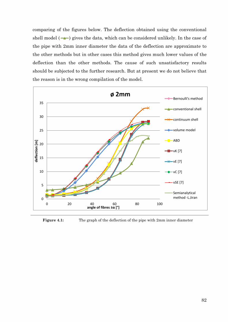
82

comparing of the figures below. The deflection obtained using the conventional

shell model ( ) gives the data, which can be considered unlikely. In the case of

the pipe with 2mm inner diameter the data of the deflection are approximate to

the other methods but in other cases this method gives much lower values of the

deflection than the other methods. The cause of such unsatisfactory results

should be subjected to the further research. But at present we do not believe that

the reason is in the wrong compilation of the model.

Figure 4.1: The graph of the deflection of the pipe with 2mm inner diameter

0

5

10

15

20

25

30

35

0 20 40 60 80 100

de

fle

ctio

n [

m]

angle of fibres ±α [°]

ø 2mm Bernoulli's method

conventional shell

continuum shell

volume model

ABD

vK [7]

vE [7]

vC [7]

vSE [7]

Semianalytical method -L.Jiran

83



0

2

4

6

8

10

12

14

0 20 40 60 80 100

de

fle

ctio

n [

m]



conventional shell

continuum shell

volume model

ABD

vK [7]

vE [7]

vC [7]

vSE [7]


0

1

2

3

4

5

6

7

0 20 40 60 80 100

de

fle

ctio

n [

m]



conventional shell

continuum shell

volume model

ABD

vK [7]

vE [7]

vC [7]

vSE [7]


84



0

0,5

1

1,5

2

2,5

3

3,5

4

0 20 40 60 80 100

de

fle

ctio

n [

m]



conventional shell

continuum shell

Volume model

ABD

vK [7]

vE [7]

vC [7]

vSE [7]


0

0,5

1

1,5

2

0 20 40 60 80 100

de

fle

ctio

n [

m]



conventional shell

continuum shell

Volume model

ABD

vK [7]

vE [7]

vC [7]

vSE [7]


85

5 Conclusion

The aim of this study was to compare the analytical methods of calculation of the

deflection of the beam with the results of the modelling of the same by using

FEM. In this thesis were compared the Bernoulli’s methods with the calculation

using ABD matrix and with the FEM models of the conventional shell, the

continuum shell and the volume model. The analytical models were performed in

MATLAB® and the FEM models were implemented in Abaqus®.

All discussed methods were applied to several beams of a circular cross section

with a different diameter and with the various layup of the composite material.

The analytical methods give the results that were expected and show a material

behaviour predicted by other theories. The FEM models give more interesting

results. Results calculated using a volume model are the closest to the results of

analytical methods. The continuum shell model gives the comparable results, but

in some cases considerably deviates from the solution calculated by analytical

methods. The conventional shell model provides the completely different

outcomes from the other methods. It is recommended for a further research.

All results were presented both graphically and in the tabular form. The

calculation methods with specific comments on the creation of individual

programs and FEM models are described in detail in this thesis. The codes in

MATLAB® and scripts of the models, which are created in Abaqus®, including

the input files are attached in the annexes.

The analysis made in this thesis does not include all the existing methods for the

calculation of the deflection of the composite materials; it would be appropriate

the extension by another methods and the concrete comparison with an

experiment would be appropriate.

86

List of Literature

[1] LAŠ, Vladislav. Mechanika kompozitních materiálů. 2. přeprac. vyd. Plzeň:

Západočeská univerzita, 2008. 200s. ISBN 978-80-7043-689-9.

[2] MICHALEC, Jiří a kol. Pružnost a pevnost I. Vyd. 3. Praha: ČVUT, 2009. 308

s. ISBN 978-80-01-04224-3.

[3] ŘEZNÍČEK, Jan a Jitka ŘEZNÍČKOVÁ. Pružnost a pevnost v technické praxi:

příklady III. Praha: Česká technika - nakladatelství ČVUT, 2008. 73 s. ISBN

978-80-01-03947-2.

[4] BARBERO, Ever J. Introduction to composite materials design. 2nd ed. Boca

Raton: Taylor & Francis, ©2011. xxxix, 520 s. ISBN 978-1-4200-7915-9.

[5] GAY, Daniel. Composite materials: design and applications. Third ed. Boca

Raton: CRC Press/Taylor & Francis, ©2015. xxiii, 611 s. ISBN 978-1-4665-8487-7.

[6] ZAVŘELOVÁ, Tereza. Model ohybu kompozitního nosníku. Praha, 2013.

Bakalářská práce. České vysoké učení technické v Praze. Fakulta strojní.

Vedoucí práce Karel DOUBRAVA.

[7] KULÍŠEK Viktor, Lukáš JIRAN, Tomáš MAREŠ, Milan RŮŽIČKA a kol.

DV#7-1 (2012) Verifikované výpočetní modely pro predikci tuhosti a modálních

vlastností komponent z nekonvenčních materiálů. Praha, 2012. Neveřejná

výzkumná zpráva č. V-12-060. ČVUT v Praze. Fakulta strojní, Ústav výrobních

strojů a zařízení.

87

List of Annexes


DP_Trubka.m 88

1.2 Program designed in MATLAB® using ABD matrices:

DP_ABD_Trubka.m 91

1.3 Script for FEM model using conventional shell 95

1.4 Script for FEM model using continuum shell 100

1.5 Script for FEM model using volume model 107

88


DP_Trubka.m

clear all close all clc %Vektor uhlu vlaken Alfa=[0 5 15 25 35 45 55 65 75 85 90]; %Vektor prumeru D=(1:20)*1e-3; %Pocet promennych K=size(D); K=K(2); Q=size(Alfa); Q=Q(2); %Pole pro vysledky V_vysledky=zeros(K,Q); W_vysledky=zeros(K,Q); for k=1:K for q=1:Q %VSTUPY %sila F [N] F=100; %GEOMETRIE %delka l [m] l=1; %polomery - vnitrni, vnejsi [m] r1=D(k)/2; %r2=(30e-3)/2; %EL, Et, Glt, vlt, alfa, t[m] v tabulce/ matici - poradi je zavazne V=[156.05e9 6.045e9 4.431e9 0.328 90 1e-3; 156.05e9 6.045e9 4.431e9 0.328 Alfa(q) 1e-3; 156.05e9 6.045e9 4.431e9 0.328 -Alfa(q) 1e-3;]; %- V jako vstupy %N- pocet vrstev N=size(V,1); %soucinitel beta beta= 1 ;

89

%pole pro ulozeni dat pro jdn. vrstvy - mozna nadbytecne E=zeros(3,3,N); T=zeros(3,3,N); %J=zeros(N,1); %Ex=zeros(N,1); Cxy=zeros(3,3,N); Gxy=zeros(N,1); A=zeros(N,1); %vsechny potrebne prumery d=zeros(N+1,1); d(1)=2*r1; for i=1:N %sestaveni Ci e11=V(i,1)/(1-(V(i,2)/V(i,1))*V(i,4)^2); e22=e11*(V(i,2)/V(i,1)); e12=V(i,4)*e22; e21=e12; e66=V(i,3); E(:,:,i)=[e11 e12 0; e21 e22 0; 0 0 e66]; %sestaveni Ti alfa=V(i,5)/180*pi; T(:,:,i)=[ (cos(alfa))^2 (sin(alfa))^2 -2*sin(alfa)*cos(alfa); (sin(alfa))^2 (cos(alfa))^2 2*sin(alfa)*cos(alfa); sin(alfa)*cos(alfa) -sin(alfa)*cos(alfa) (cos(alfa))^2-(sin(alfa))^2]; %sestaveni Ji d(i+1)=d(i)+2*V(i,6); J(i)=(pi*(d(i+1)^4/64))*(1-(d(i)/d(i+1))^4); %transformace Ei do systemu xy Exy(:,:,i)=T(:,:,i)*E(:,:,i)*T(:,:,i)'; %Matice poddajnosti Cxy(:,:,i)=inv(Exy(:,:,i)); %Vektor hodnot modulu pruznosti v tahu Exi =[Ex1 Ex2 ....ExN] exi=1/Cxy(1,1,i); Ex(i)=exi;

90

%plocha pro Gxy*A A(i)=(pi()/4)*(d(i+1)^2-d(i)^2); %modul pruznosti ve smyku gxyi=1/Cxy(3,3,i); Gxy(i)=gxyi; end %Ohybova tuhost EJ=Ex*J' ;%vychazim z toho, ze fce zeros generuje radkove vektory(?) %Soucin Gxy*A GxyA=Gxy'*A; %beta/Gxy*A betaGA=beta./GxyA; %PRUHYB x=0:l/10:l; %vypocet Mohr. integral v=(1/EJ)*((F*l^2*x)-(F*l*x.^2)-(F*x.^3)/3); %vypocet se zahrnutim smyku w=(1/EJ)*((F*l^2*x)-(F*l*x.^2)-(F*x.^3)/3)+betaGA*F*x; %Tabulky vysledku - matice V_vysledky(k,q)=v(1); W_vysledky(k,q)=w(1); end end %save ('DP_Trubka_uhly_prumery', 'V_vysledky', 'W_vysledky' )

91

1.2 Program designed in MATLAB® using ABD matrices: DP_ABD_Trubka.m clc clear all close all %% Vstupy %Vektor uhlu vlaken Alfa=[0 5 15 25 35 45 55 65 75 85 90]; %Vektor prumeru P=(1:10)*1e-3; %Pocet promennych K=size(P); K=K(2); U=size(Alfa); U=U(2); %Pole pro vysledky V_vysledky=zeros(K,U); W_vysledky=zeros(K,U); for s=1:K for t=1:U %VSTUPZ %Sila F=100; %GEOMETRIE %delka l [m] l=1; %polomery - vnitrni, vnejsi [m] r1=P(s)/2; %r2=(30e-3)/2; % Matice vstupu pro jdntl. vrstvy % 1 2 3 4 5 6 % EL ET GLT vLT alfa(°) t(m) V=[156.05e9 6.045e9 4.431e9 0.328 90 1e-3; 156.05e9 6.045e9 4.431e9 0.328 Alfa(t) 1e-3; 156.05e9 6.045e9 4.431e9 0.328 -Alfa(t) 1e-3;]; %- V jako vstupy %pocet vrstev k xx=size(V); k=xx(1);

92

%pole pro ukladani mezivypoctu Tvx=zeros(6,6,k); c=zeros(6,6,k); C=zeros(3,3,k); Cxy=zeros(3,3,k); Q=zeros(3,3,k); q=zeros(6,6,k); A=zeros(3,3); B=zeros(3,3); D=zeros(3,3); %% Matice tuhosti for i=1:k c(1,1,i)=V(i,1)/(1-((V(i,2)/V(i,1))*V(i,4)^2)); c(2,2,i)=V(i,2)/V(i,1)*c(1,1,i); c(1,2,i)=V(i,4)*c(2,2,i); c(2,1,i)=c(1,2,i); c(6,6,i)=V(i,3); C(:,:,i)=[c(1,1,i) c(1,2,i) 0; c(2,1,i) c(2,2,i) 0; 0 0 c(6,6,i);]; %% Transformace matice tuhosti % Transformacni matice ze systemu LTt do systemu xyz alfa=V(i,5)/180*pi; Ts(:,:,i)=[ (cos(alfa))^2 (sin(alfa))^2 2*sin(alfa)*cos(alfa); (sin(alfa))^2 (cos(alfa))^2 -2*sin(alfa)*cos(alfa); -sin(alfa)*cos(alfa) sin(alfa)*cos(alfa) (cos(alfa))^2-(sin(alfa))^2]; Te(:,:,i)=[ (cos(alfa))^2 (sin(alfa))^2 sin(alfa)*cos(alfa); (sin(alfa))^2 (cos(alfa))^2 -sin(alfa)*cos(alfa); -2*sin(alfa)*cos(alfa) 2*sin(alfa)*cos(alfa) (cos(alfa))^2-(sin(alfa))^2]; Cxy(:,:,i)=inv(Ts(:,:,i))*C(:,:,i)*Te(:,:,i);%(Tvx)^-1*C*Tvx' ????? \Tvx !!!!!=Q pro rovinnou napjatost end %% Matice ABD h(1)=-sum(V(:,6))/2;%h0 for n=1:k; for m=1:k; for i=1:k; %Vsechna h h(i+1)=(h(1)+sum(V(1:i,6)));

93

a(i)=(Cxy(n,m,i)*(h(i+1)-h(i))); b(i)=((1/2)*Cxy(n,m,i)*(h(i+1)^2-h(i)^2)); d(i)=((1/3)*Cxy(n,m,i)*(h(i+1)^3-h(i)^3)); end A(n,m)=sum(a); B(n,m)=sum(b); D(n,m)=sum(d); end end %Modul pruznosti v tahu E=(A(1,1)-A(1,2:3)*(A(2:3,2:3)^(-1)*A(2:3,1)))/sum(V(:,6)); %Modul pruznosti ve smyku G=(A(3,3)-A(3,1:2)*(A(1:2,1:2)^(-1)*A(1:2,3)))/sum(V(:,6)); %vsechny potrebne prumery dd=zeros(k+1,1); dd(1)=2*r1; %sestaveni Ji a GA for i=1:k dd(i+1)=dd(i)+2*V(i,6); j(i)=(pi*(dd(i+1)^4/64))*(1-(dd(i)/dd(i+1))^4); %plocha pro G*A S(i)=(pi/4)*(dd(i+1)^2-dd(i)^2); %modul pruznosti ve smyku % gxyi=1/Cxy(6,6,i); % Gxy(i)=gxyi; end J=sum(j); S_celk=sum(S); %PRUHYB x=0:l/10:l; %vypocet Mohr. integral v=(1/(E*J))*((F*l^3)/3-(F*l^2*x)/2-(F*x.^3)/3+(F*x.^3)/2); %vypocet se zahrnutim smyku %soucinitel beta beta= 1 ;

94

%Soucin Gxy*A GxyA=G*S_celk; %beta/Gxy*A betaGA=beta/GxyA; w=(1/(E*J))*((F*l^3)/3-(F*l^2*x)/2-(F*x.^3)/3+(F*x.^3)/2)+betaGA*F*(l-x); %Tabulky vysledku - matice V_vysledky_G(s,t)=v(1); W_vysledky_G(s,t)=w(1); end end save('DP_ABD_Trubka_uhly_prumery', 'V_vysledky_G', 'W_vysledky_G')

95

1.3 Script for FEM model using conventional shell

#prumer

d=0.008

x=d*0.1

r=d/2

#uhel

a=0

# -*- coding: mbcs -*-

from part import *

from material import *

from section import *

from assembly import *

from step import *

from interaction import *

from load import *

from mesh import *

from optimization import *

from job import *

from sketch import *

from visualization import *

from connectorBehavior import *

mdb.models['Model-1'].ConstrainedSketch(name='__profile__', sheetSize=2.0)

mdb.models['Model-1'].sketches['__profile__'].CircleByCenterPerimeter(center=(

0.0, 0.0), point1=(-0.1, 0.0))

mdb.models['Model-1'].sketches['__profile__'].RadialDimension(curve=

mdb.models['Model-1'].sketches['__profile__'].geometry[2], radius=0.005,

textPoint=(0.0, 0.0))

mdb.models['Model-1'].sketches['__profile__'].delete(objectList=(

mdb.models['Model-1'].sketches['__profile__'].dimensions[0], ))


mdb.models['Model-1'].sketches['__profile__'].geometry[2], radius=r,


mdb.models['Model-1'].Part(dimensionality=THREE_D, name='Part-1', type=

DEFORMABLE_BODY)

mdb.models['Model-1'].parts['Part-1'].BaseShellExtrude(depth=1.0, sketch=

mdb.models['Model-1'].sketches['__profile__'])

del mdb.models['Model-1'].sketches['__profile__']

mdb.models['Model-1'].parts['Part-1'].DatumCsysByThreePoints(coordSysType=

CARTESIAN, name='Datum csys-1', origin=

mdb.models['Model-1'].parts['Part-1'].InterestingPoint(

mdb.models['Model-1'].parts['Part-1'].edges[0], CENTER), point1=




mdb.models['Model-1'].parts['Part-1'].edges[0], MIDDLE))

96

mdb.models['Model-1'].Material(name='Material-1')

mdb.models['Model-1'].materials['Material-1'].Density(table=((1474.0, ), ))

mdb.models['Model-1'].materials['Material-1'].Elastic(table=((156050000000.0,

6045000000.0, 0.328, 4431000000.0, 4431000000.0, 4431000000.0), ), type=

LAMINA)

mdb.models['Model-1'].parts['Part-1'].DatumPlaneByThreePoints(point1=

mdb.models['Model-1'].parts['Part-1'].vertices[0], point2=


mdb.models['Model-1'].parts['Part-1'].edges[0], MIDDLE), point3=



mdb.models['Model-1'].parts['Part-1'].PartitionFaceByDatumPlane(datumPlane=

mdb.models['Model-1'].parts['Part-1'].datums[3], faces=

mdb.models['Model-1'].parts['Part-1'].faces.getSequenceFromMask(('[#1 ]', ),

))

mdb.models['Model-1'].parts['Part-1'].CompositeLayup(description='',

elementType=SHELL, name='CompositeLayup-1',

offsetType=BOTTOM_SURFACE,

symmetric=False, thicknessAssignment=FROM_SECTION)

mdb.models['Model-1'].parts['Part-1'].compositeLayups['CompositeLayup-

1'].Section(

integrationRule=SIMPSON, poissonDefinition=DEFAULT, preIntegrate=OFF,

temperature=GRADIENT, thicknessType=UNIFORM, useDensity=OFF)


1'].ReferenceOrientation(

additionalRotationField='', additionalRotationType=ROTATION_NONE,

angle=0.0

, axis=AXIS_2, fieldName='', localCsys=

mdb.models['Model-1'].parts['Part-1'].datums[2], orientationType=SYSTEM)


1'].CompositePly(

additionalRotationField='', additionalRotationType=ROTATION_ANGLE,

angle=

90.0, axis=AXIS_2, material='Material-1', numIntPoints=3, orientation=

mdb.models['Model-1'].parts['Part-1'].datums[2], orientationType=CSYS,

plyName='Ply-1', region=Region(

faces=mdb.models['Model-1'].parts['Part-1'].faces.getSequenceFromMask(

mask=('[#3 ]', ), )), suppressed=False, thickness=0.001, thicknessType=

SPECIFY_THICKNESS)


1'].CompositePly(


angle=a

, axis=AXIS_2, material='Material-1', numIntPoints=3, orientation=

97





SPECIFY_THICKNESS)


1'].CompositePly(


angle=-a






SPECIFY_THICKNESS)

mdb.models['Model-1'].rootAssembly.DatumCsysByDefault(CARTESIAN)

mdb.models['Model-1'].rootAssembly.Instance(dependent=OFF, name='Part-1-1',

part=mdb.models['Model-1'].parts['Part-1'])

mdb.models['Model-1'].StaticStep(name='Step-1', previous='Initial')

mdb.models['Model-1'].rootAssembly.ReferencePoint(point=

mdb.models['Model-1'].rootAssembly.instances['Part-1-1'].InterestingPoint(

mdb.models['Model-1'].rootAssembly.instances['Part-1-1'].edges[3], CENTER))

mdb.models['Model-1'].rootAssembly.Set(name='m_Set-1', referencePoints=(

mdb.models['Model-1'].rootAssembly.referencePoints[4], ))

mdb.models['Model-1'].rootAssembly.Set(edges=

mdb.models['Model-1'].rootAssembly.instances['Part-1-

1'].edges.getSequenceFromMask(

('[#18 ]', ), ), name='s_Set-1')

mdb.models['Model-1'].Coupling(controlPoint=

mdb.models['Model-1'].rootAssembly.sets['m_Set-1'],

couplingType=KINEMATIC,

influenceRadius=WHOLE_SURFACE, localCsys=

mdb.models['Model-1'].rootAssembly.instances['Part-1-1'].datums[2], name=

'Constraint-1', surface=mdb.models['Model-1'].rootAssembly.sets['s_Set-1'],

u1=ON, u2=ON, u3=ON, ur1=ON, ur2=ON, ur3=ON)

mdb.models['Model-1'].fieldOutputRequests['F-Output-1'].setValues(variables=(

'U', 'UT', 'UR'))

mdb.models['Model-1'].rootAssembly.Set(name='Set-3', referencePoints=(


mdb.models['Model-1'].ConcentratedForce(cf3=100.0, createStepName='Step-1',

distributionType=UNIFORM, field='', localCsys=


'Load-1', region=mdb.models['Model-1'].rootAssembly.sets['Set-3'])

mdb.models['Model-1'].rootAssembly.Set(edges=



('[#22 ]', ), ), name='Set-4')

mdb.models['Model-1'].EncastreBC(createStepName='Step-1', localCsys=

98


'BC-1', region=mdb.models['Model-1'].rootAssembly.sets['Set-4'])

mdb.models['Model-1'].rootAssembly.setElementType(elemTypes=(ElemType(

elemCode=S4R, elemLibrary=STANDARD, secondOrderAccuracy=OFF,

hourglassControl=DEFAULT), ElemType(elemCode=S3,

elemLibrary=STANDARD)),

regions=(


1'].faces.getSequenceFromMask(

('[#3 ]', ), ), ))

mdb.models['Model-1'].rootAssembly.setMeshControls(regions=



('[#3 ]', ), ), technique=STRUCTURED)

mdb.models['Model-1'].rootAssembly.seedPartInstance(deviationFactor=0.1,

minSizeFactor=0.1, regions=(

mdb.models['Model-1'].rootAssembly.instances['Part-1-1'], ), size=0.005)

mdb.models['Model-1'].rootAssembly.seedEdgeBySize(constraint=FINER,

deviationFactor=0.1, edges=



('[#3a ]', ), ), minSizeFactor=0.1, size=x)

mdb.models['Model-1'].rootAssembly.generateMesh(regions=(

mdb.models['Model-1'].rootAssembly.instances['Part-1-1'], ))

mdb.Job(atTime=None, contactPrint=OFF, description='', echoPrint=OFF,

explicitPrecision=SINGLE, getMemoryFromAnalysis=True, historyPrint=OFF,

memory=50, memoryUnits=PERCENTAGE, model='Model-1',

modelPrint=OFF,

multiprocessingMode=DEFAULT, name='Job-0',

nodalOutputPrecision=SINGLE,

numCpus=1, numGPUs=0, queue=None, scratch='', type=ANALYSIS,

userSubroutine='', waitHours=0, waitMinutes=0)

mdb.jobs['Job-0'].submit(consistencyChecking=OFF)

mdb.jobs['Job-0']._Message(STARTED, {'phase': BATCHPRE_PHASE,

'clientHost': 'ntb-HPPB4310s', 'handle': 0, 'jobName': 'Job-0'})

mdb.jobs['Job-0']._Message(WARNING, {'phase': BATCHPRE_PHASE,

'message': 'WHENEVER A TRANSLATION (ROTATION) DOF AT A NODE IS

CONSTRAINED BY A KINEMATIC COUPLING DEFINITION THE

TRANSLATION (ROTATION) DOFS FOR THAT NODE CANNOT BE

INCLUDED IN ANY OTHER CONSTRAINT INCLUDING MPCS, RIGID

BODIES, ETC.',

'jobName': 'Job-0'})

mdb.jobs['Job-0']._Message(WARNING, {'phase': BATCHPRE_PHASE,

'message': 'MPCS (EXTERNAL or INTERNAL, including those generated from

rigid body definitions), KINEMATIC COUPLINGS, AND/OR EQUATIONS WILL

ACTIVATE ADDITIONAL DEGREES OF FREEDOM',


99

mdb.jobs['Job-0']._Message(ODB_FILE, {'phase': BATCHPRE_PHASE,

'file': 'C:\\Temp\\Job-0.odb', 'jobName': 'Job-0'})

mdb.jobs['Job-0']._Message(COMPLETED, {'phase': BATCHPRE_PHASE,

'message': 'Analysis phase complete', 'jobName': 'Job-0'})

mdb.jobs['Job-0']._Message(STARTED, {'phase': STANDARD_PHASE,

'clientHost': 'ntb-HPPB4310s', 'handle': 5316, 'jobName': 'Job-0'})

mdb.jobs['Job-0']._Message(STEP, {'phase': STANDARD_PHASE, 'stepId': 1,


mdb.jobs['Job-0']._Message(WARNING, {'phase': STANDARD_PHASE,

'message': 'The 3-direction at one or more points in one or more layers in 3200

elements as defined in *ORIENTATION are in the opposite direction to the

element normals. Either the 1 or 2 and the 3-direction defined in

*ORIENTATION will be reversed. The elements have been identified in element

set WarnElem3DirOppElemNormalStep1Inc1.',


mdb.jobs['Job-0']._Message(ODB_FRAME, {'phase': STANDARD_PHASE, 'step':

0,

'frame': 0, 'jobName': 'Job-0'})

mdb.jobs['Job-0']._Message(STATUS, {'totalTime': 0.0, 'attempts': 0,

'timeIncrement': 1.0, 'increment': 0, 'stepTime': 0.0, 'step': 1,

'jobName': 'Job-0', 'severe': 0, 'iterations': 0, 'phase': STANDARD_PHASE,

'equilibrium': 0})

mdb.jobs['Job-0']._Message(MEMORY_ESTIMATE, {'phase':

STANDARD_PHASE,

'jobName': 'Job-0', 'memory': 132.121262550354})

mdb.jobs['Job-0']._Message(ODB_FRAME, {'phase': STANDARD_PHASE, 'step':

0,

'frame': 1, 'jobName': 'Job-0'})

mdb.jobs['Job-0']._Message(STATUS, {'totalTime': 1.0, 'attempts': 1,


'jobName': 'Job-0', 'severe': 0, 'iterations': 2, 'phase': STANDARD_PHASE,

'equilibrium': 2})

mdb.jobs['Job-0']._Message(END_STEP, {'phase': STANDARD_PHASE, 'stepId':

1,


mdb.jobs['Job-0']._Message(COMPLETED, {'phase': STANDARD_PHASE,

'message': 'Analysis phase complete', 'jobName': 'Job-0'})

mdb.jobs['Job-0']._Message(JOB_COMPLETED, {'time': 'Thu Mar 12 16:21:06

2015',


# Save by user on 2015_03_12-16.23.10; build 6.12-1 2012_03_13-20.44.39 119612

100

1.4 Script for FEM model using continuum shell

#prumer

d=0.002

r=d/2

k=r+0.003

#uhel

a=90


from part import *





from step import *


from load import *

from mesh import *

from job import *






0.0, 0.0), point1=(-2.5, 0.0))


0.0, 0.0), point1=(-1.25, 0.0))


mdb.models['Model-1'].sketches['__profile__'].geometry[2], radius=r,



mdb.models['Model-1'].sketches['__profile__'].geometry[3], radius=k,



DEFORMABLE_BODY)

mdb.models['Model-1'].parts['Part-1'].BaseSolidExtrude(depth=1.0, sketch=






6045000000.0, 0.328, 4431000000.0, 4431000000.0, 4431000000.0), ), type=

LAMINA)

101

mdb.models['Model-1'].parts['Part-1'].DatumPlaneByThreePoints(point1=

mdb.models['Model-1'].parts['Part-1'].vertices[2], point2=


mdb.models['Model-1'].parts['Part-1'].edges[2], MIDDLE), point3=



mdb.models['Model-1'].parts['Part-1'].PartitionCellByDatumPlane(cells=

mdb.models['Model-1'].parts['Part-1'].cells.getSequenceFromMask(('[#1 ]',

), ), datumPlane=mdb.models['Model-1'].parts['Part-1'].datums[2])









mdb.models['Model-1'].parts['Part-1'].CompositeLayup(description='',

elementType=CONTINUUM_SHELL, name='CompositeLayup-1',

symmetric=False)


1'].Section(

integrationRule=SIMPSON, poissonDefinition=DEFAULT, preIntegrate=OFF,

temperature=GRADIENT, thicknessModulus=None, useDensity=OFF)


1'].ReferenceOrientation(


angle=0.0


mdb.models['Model-1'].parts['Part-1'].datums[4], orientationType=SYSTEM,

stackDirection=STACK_3)


1'].CompositePly(


angle=0.0




cells=mdb.models['Model-1'].parts['Part-1'].cells.getSequenceFromMask(


SPECIFY_THICKNESS)

102


1'].CompositePly(


angle=0.0






SPECIFY_THICKNESS)


1'].CompositePly(


angle=0.0






SPECIFY_THICKNESS)






'U', 'UT', 'UR', 'RF', 'CF'))






mdb.models['Model-1'].rootAssembly.Surface(name='s_Surf-1', side1Faces=



('[#204 ]', ), ))






'Constraint-1', surface=

mdb.models['Model-1'].rootAssembly.surfaces['s_Surf-1'], u1=ON, u2=ON, u3=

ON, ur1=ON, ur2=ON, ur3=ON)

mdb.models['Model-1'].rootAssembly.Set(faces=



('[#110 ]', ), ), name='Set-2')

103

mdb.models['Model-1'].EncastreBC(createStepName='Step-1', localCsys=


'BC-1', region=mdb.models['Model-1'].rootAssembly.sets['Set-2'])






'Load-1', region=mdb.models['Model-1'].rootAssembly.sets['Set-3'])

mdb.models['Model-1'].rootAssembly.setElementType(elemTypes=(ElemType(

elemCode=SC8R, elemLibrary=STANDARD, secondOrderAccuracy=OFF,

hourglassControl=DEFAULT), ElemType(elemCode=SC6R,

elemLibrary=STANDARD),

ElemType(elemCode=UNKNOWN_TET, elemLibrary=STANDARD)),

regions=(


1'].cells.getSequenceFromMask(

('[#3 ]', ), ), ))











('[#3ff00 ]', ), ), minSizeFactor=0.1, size=0.001)


















104





mdb.models['Model-1'].rootAssembly.instances['Part-1-1'], ))


1'].deletePlies( )


1'].CompositePly(

additionalRotationField='', additionalRotationType=ROTATION_ANGLE,

angle=

90.0, axis=AXIS_2, material='Material-1', numIntPoints=3, orientation=





SPECIFY_THICKNESS)


1'].CompositePly(


angle=a






SPECIFY_THICKNESS)


1'].CompositePly(


angle=-a






SPECIFY_THICKNESS)

mdb.models['Model-1'].rootAssembly.regenerate()




modelPrint=OFF,

multiprocessingMode=DEFAULT, name='Job-e',




mdb.jobs['Job-e'].submit(consistencyChecking=OFF)

mdb.jobs['Job-e']._Message(STARTED, {'phase': BATCHPRE_PHASE,

105

'clientHost': 'ntb-HPPB4310s', 'handle': 0, 'jobName': 'Job-e'})

mdb.jobs['Job-e']._Message(WARNING, {'phase': BATCHPRE_PHASE,

'message': 'WHENEVER A TRANSLATION (ROTATION) DOF AT A NODE IS

CONSTRAINED BY A KINEMATIC COUPLING DEFINITION THE

TRANSLATION (ROTATION) DOFS FOR THAT NODE CANNOT BE

INCLUDED IN ANY OTHER CONSTRAINT INCLUDING MPCS, RIGID

BODIES, ETC.',

'jobName': 'Job-e'})

mdb.jobs['Job-e']._Message(WARNING, {'phase': BATCHPRE_PHASE,

'message': 'MPCS (EXTERNAL or INTERNAL, including those generated from

rigid body definitions), KINEMATIC COUPLINGS, AND/OR EQUATIONS WILL

ACTIVATE ADDITIONAL DEGREES OF FREEDOM',


mdb.jobs['Job-e']._Message(ODB_FILE, {'phase': BATCHPRE_PHASE,

'file': 'C:\\Temp\\Job-e.odb', 'jobName': 'Job-e'})

mdb.jobs['Job-e']._Message(COMPLETED, {'phase': BATCHPRE_PHASE,

'message': 'Analysis phase complete', 'jobName': 'Job-e'})

mdb.jobs['Job-e']._Message(STARTED, {'phase': STANDARD_PHASE,

'clientHost': 'ntb-HPPB4310s', 'handle': 3840, 'jobName': 'Job-e'})

mdb.jobs['Job-e']._Message(STEP, {'phase': STANDARD_PHASE, 'stepId': 1,


mdb.jobs['Job-e']._Message(WARNING, {'phase': STANDARD_PHASE,

'message': 'The 3-direction at one or more points in one or more layers in 8200

elements as defined in *ORIENTATION are in the opposite direction to the

element normals. Either the 1 or 2 and the 3-direction defined in

*ORIENTATION will be reversed. The elements have been identified in element

set WarnElem3DirOppElemNormalStep1Inc1.',


mdb.jobs['Job-e']._Message(ODB_FRAME, {'phase': STANDARD_PHASE, 'step':

0,

'frame': 0, 'jobName': 'Job-e'})

mdb.jobs['Job-e']._Message(STATUS, {'totalTime': 0.0, 'attempts': 0,


'jobName': 'Job-e', 'severe': 0, 'iterations': 0, 'phase': STANDARD_PHASE,

'equilibrium': 0})

mdb.jobs['Job-e']._Message(MEMORY_ESTIMATE, {'phase':

STANDARD_PHASE,

'jobName': 'Job-e', 'memory': 348.168928146362})

mdb.jobs['Job-e']._Message(ODB_FRAME, {'phase': STANDARD_PHASE, 'step':

0,

'frame': 1, 'jobName': 'Job-e'})

mdb.jobs['Job-e']._Message(STATUS, {'totalTime': 1.0, 'attempts': 1,


'jobName': 'Job-e', 'severe': 0, 'iterations': 1, 'phase': STANDARD_PHASE,

'equilibrium': 1})

mdb.jobs['Job-e']._Message(END_STEP, {'phase': STANDARD_PHASE, 'stepId':

1,


106

mdb.jobs['Job-e']._Message(COMPLETED, {'phase': STANDARD_PHASE,

'message': 'Analysis phase complete', 'jobName': 'Job-e'})

mdb.jobs['Job-e']._Message(JOB_COMPLETED, {'time': 'Wed Mar 11 14:48:04

2015',



107

1.5 Script for FEM model using volume model

#prumer

d=0.01

#uhel

a=55

#polomery

r1=d/2

r2=r1+0.001

r3=r2+0.001

r4=r3+0.001

x1=d*0.1

# -*- coding: mbcs -*-

from part import *




from step import *


from load import *

from mesh import *


from job import *





mdb.models['Model-1'].sketches['__profile__'].sketchOptions.setValues(

decimalPlaces=3)


0.0, 0.0), point1=(-0.005, 0.0))


0.0, 0.0), point1=(-0.01, 0.0))


mdb.models['Model-1'].sketches['__profile__'].geometry[2], radius=r1,






DEFORMABLE_BODY)



108




decimalPlaces=3)


0.0, 0.0), point1=(-0.005, 0.0))


0.0, 0.0), point1=(-0.01, 0.0))








DEFORMABLE_BODY)






decimalPlaces=3)


0.0, 0.0), point1=(-0.005, 0.0))


0.0, 0.0), point1=(-0.01, 0.0))








DEFORMABLE_BODY)







6045000000.0, 6045000000.0, 0.328, 0.328, 0.328, 4431000000.0,

4431000000.0, 4431000000.0), ), type=ENGINEERING_CONSTANTS)

mdb.models['Model-1'].CompositeSolidSection(layup=(SectionLayer(

thickness=0.001, orientAngle=90.0, numIntPts=1, material='Material-1',

plyName='Ply-1'), ), layupName='', name='Section-1', symmetric=False)


thickness=0.001, orientAngle=a, numIntPts=1, material='Material-1',


109


thickness=0.001, orientAngle=-a, numIntPts=1, material='Material-1',


























mdb.models['Model-1'].parts['Part-1'].MaterialOrientation(


angle=0.0



region=Region(


mask=('[#1 ]', ), )), stackDirection=STACK_3)



angle=0.0



region=Region(





angle=0.0


110


region=Region(



mdb.models['Model-1'].parts['Part-1'].Set(cells=


), ), name='Set-2')

mdb.models['Model-1'].parts['Part-1'].SectionAssignment(offset=0.0,

offsetField='', offsetType=MIDDLE_SURFACE, region=

mdb.models['Model-1'].parts['Part-1'].sets['Set-2'], sectionName=

'Section-1', thicknessAssignment=FROM_SECTION)



), ), name='Set-2')







), ), name='Set-2')












mdb.models['Model-1'].rootAssembly.Coaxial(fixedAxis=

mdb.models['Model-1'].rootAssembly.instances['Part-2-1'].faces[1], flip=OFF

, movableAxis=

mdb.models['Model-1'].rootAssembly.instances['Part-1-1'].faces[1])



, movableAxis=




, movableAxis=


mdb.models['Model-1'].rootAssembly.ParallelFace(fixedPlane=


, movablePlane=


111

mdb.models['Model-1'].rootAssembly.ParallelFace(fixedPlane=


, movablePlane=


mdb.models['Model-1'].rootAssembly.DatumPlaneByThreePoints(point1=

mdb.models['Model-1'].rootAssembly.instances['Part-3-1'].vertices[0],

point2=


mdb.models['Model-1'].rootAssembly.instances['Part-3-1'].edges[0], MIDDLE),

point3=


mdb.models['Model-1'].rootAssembly.instances['Part-3-1'].edges[1], MIDDLE))

mdb.models['Model-1'].rootAssembly.PartitionCellByDatumPlane(cells=



mask=('[#1 ]', ), )+\



mask=('[#1 ]', ), )+\



mask=('[#1 ]', ), ), datumPlane=

mdb.models['Model-1'].rootAssembly.datums[13])

mdb.models['Model-1'].rootAssembly.DatumCsysByThreePoints(coordSysType=



mdb.models['Model-1'].rootAssembly.instances['Part-3-1'].edges[10], CENTER)

, point1=


mdb.models['Model-1'].rootAssembly.instances['Part-3-1'].edges[8], CENTER),

point2=

mdb.models['Model-1'].rootAssembly.instances['Part-3-1'].vertices[0])



'U', ))






mdb.models['Model-1'].rootAssembly.Surface(name='s_Surf-1', side1Faces=



mask=('[#204 ]', ), )+\



mask=('[#204 ]', ), )+\

112



mask=('[#204 ]', ), ))





mdb.models['Model-1'].rootAssembly.datums[15], name='Constraint-1',

surface=mdb.models['Model-1'].rootAssembly.surfaces['s_Surf-1'], u1=ON, u2=

ON, u3=ON, ur1=ON, ur2=ON, ur3=ON)





mdb.models['Model-1'].rootAssembly.datums[15], name='Load-1', region=

mdb.models['Model-1'].rootAssembly.sets['Set-2'])

mdb.models['Model-1'].rootAssembly.Set(faces=



mask=('[#110 ]', ), )+\



mask=('[#110 ]', ), )+\



mask=('[#110 ]', ), ), name='Set-3')

mdb.models['Model-1'].EncastreBC(createStepName='Initial', localCsys=

mdb.models['Model-1'].rootAssembly.datums[15], name='BC-1', region=

mdb.models['Model-1'].rootAssembly.sets['Set-3'])



mdb.models['Model-1'].rootAssembly.instances['Part-3-1'],


mdb.models['Model-1'].rootAssembly.instances['Part-1-1']), size=0.005)





mask=('[#aa ]', ), )+\



mask=('[#aa ]', ), )+\



mask=('[#aa ]', ), ), minSizeFactor=0.1, size=0.0002)

113

mdb.models['Model-1'].rootAssembly.seedEdgeByNumber(constraint=FINER,

edges=



('[#a900 ]', ), ), number=20)


edges=



('[#a900 ]', ), ), number=20)


edges=



('[#a900 ]', ), ), number=20)


edges=



('[#5600 ]', ), ), number=20)




mdb.models['Model-1'].rootAssembly.instances['Part-1-1']))




modelPrint=OFF,

multiprocessingMode=DEFAULT, name='Job-55',




mdb.jobs['Job-55'].submit(consistencyChecking=OFF)

Documents

DIPLOMOVÁ PRÁCE - cvut.czusers.fs.cvut.cz/tomas.mares/theses/TerezaZavrelova2015.pdf · DIPLOMOVÁ PRÁCE Analysis of the ... 1.3 Script for FEM model using conventional shell 95