2 2 2 | N A T U R E | V O L 5 3 4 | 9 J U N E 2 0 1 6

LETTERdoi:10.1038/nature17658

Digitized adiabatic quantum computing with a superconducting circuitR. Barends1, A. Shabani2, L. Lamata3, J. Kelly1, A. Mezzacapo3†, U. Las Heras3, R. Babbush2, A. G. Fowler1, B. Campbell4, Yu Chen1, Z. Chen4, B. Chiaro4, A. Dunsworth4, E. Jeffrey1, E. Lucero1, A. Megrant4, J. Y. Mutus1, M. Neeley1, C. Neill4, P. J. J. O’Malley4, C. Quintana4, P. Roushan1, D. Sank1, A. Vainsencher4, J. Wenner4, T. C. White4, E. Solano3,5, H. Neven2 & John M. Martinis1,4

Quantum mechanics can help to solve complex problems in physics1 and chemistry2, provided they can be programmed in a physical device. In adiabatic quantum computing3–5, a system is slowly evolved from the ground state of a simple initial Hamiltonian to a final Hamiltonian that encodes a computational problem. The appeal of this approach lies in the combination of simplicity and generality; in principle, any problem can be encoded. In practice, applications are restricted by limited connectivity, available interactions and noise. A complementary approach is digital quantum computing6, which enables the construction of arbitrary interactions and is compatible with error correction7,8, but uses quantum circuit algorithms that are problem-specific. Here we combine the advantages of both approaches by implementing digitized adiabatic quantum computing in a superconducting system. We tomographically probe the system during the digitized evolution and explore the scaling of errors with system size. We then let the full system find the solution to random instances of the one-dimensional Ising problem as well as problem Hamiltonians that involve more complex interactions. This digital quantum simulation9–12 of the adiabatic algorithm consists of up to nine qubits and up to 1,000 quantum logic gates. The demonstration of digitized adiabatic quantum computing in the solid state opens a path to synthesizing long-range correlations and solving complex computational problems. When combined with fault-tolerance, our approach becomes a general-purpose algorithm that is scalable.

A key challenge in adiabatic quantum computing is to construct a device that is capable of encoding problem Hamiltonians that are classically intractable, that is, non-stoquastic13. Such Hamiltonians would enable universal adiabatic quantum computing14,15 and improve the performance for difficult instances of classical opti-mization problems16. Additionally, simulating interacting fermions for applications in physics and chemistry requires non-stoquastic Hamiltonians1,17. In general, these Hamiltonians are more difficult to study classically, because Monte Carlo simulations fail to con-verge owing to the ‘sign problem’18. A hallmark of non-stoquastic Hamiltonians is the need for several distinct types of coupling, for example, σzσz and σxσx couplings with different signs, where σx and σz are Pauli operators. With a digitized approach, different couplings can be constructed without change of hardware. Long-range multibody interactions can be assembled to aid in quan-tum tunnelling19 or to encode the non-local terms for fermionic simulations20,21. And finally, analogue systems exhibit noise, which can thwart the evolution, whereas digital systems can be fully fault-tolerant. Crucially, this ability makes the digitized approach scalable, because any non-corrected implementation is ultimately limited by the accumulation of error. Our experiment addresses the

challenge of adiabatically evolving to final problem Hamiltonians that are non-stoquastic.

We explore the adiabatic quantum evolutions of one-dimensional spin chains with nearest-neighbour coupling. We start with a simple ferromagnetic problem to visualize the adiabatic evolution process. We identify specific error contributions, and follow up by exploring the scaling of errors with system size. We finish by testing the device on random stoquastic and non-stoquastic problems. The initial (‘I’) and problem (‘P’) Hamiltonians are

( ) ( )∑

∑ ∑

σ

σ σ σ σ σ σ

=−

=− + − ++ + + +

H B

H B B J J

xi

xi

izi

zi

xi

xi

izzi i

zi

zi

xxi i

xi

xi

I ,I

P, 1 1 , 1 1

where Bzi and Bx

i denote local field strengths of the ith qubit, +J zzi i, 1 and

+J xxi i, 1 denote the σzσz and σxσx coupling strengths, respectively, between

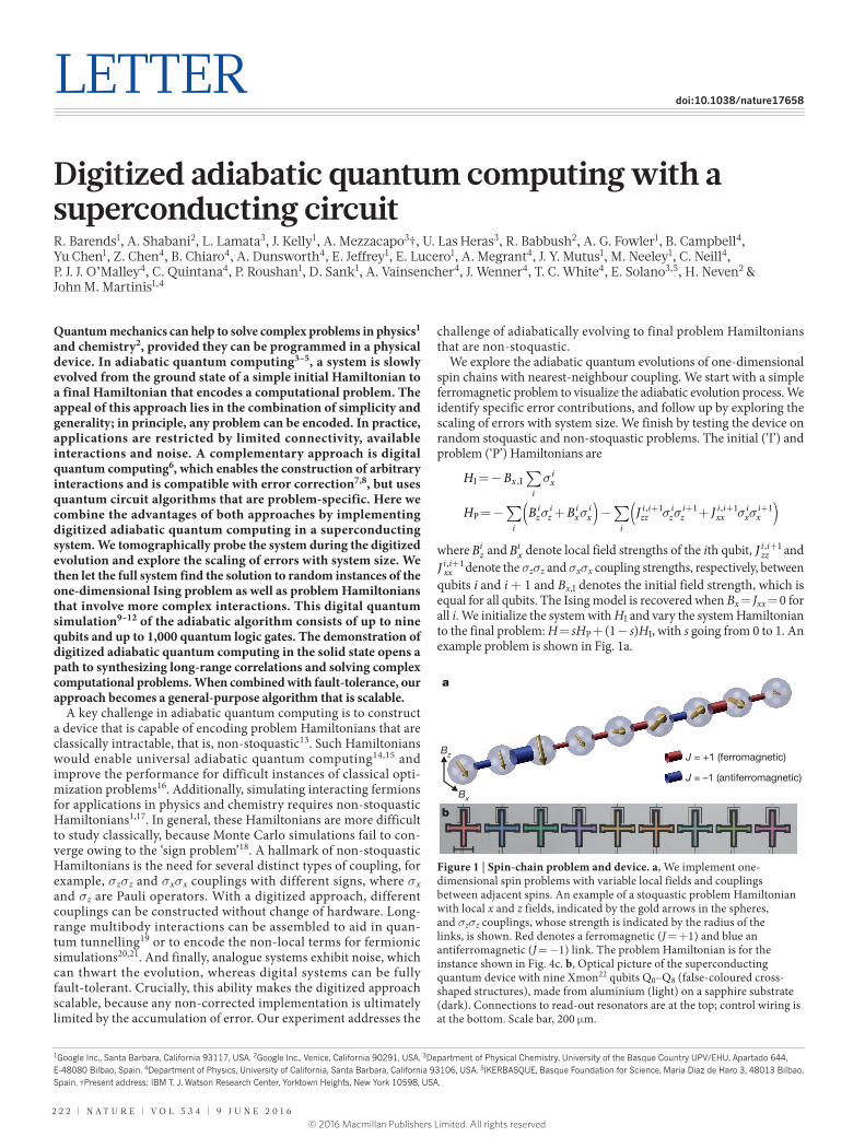
qubits i and i +  1 and Bx,I denotes the initial field strength, which is equal for all qubits. The Ising model is recovered when Bx = Jxx = 0 for all i. We initialize the system with HI and vary the system Hamiltonian to the final problem: H = sHP + (1 − s)HI, with s going from 0 to 1. An example problem is shown in Fig. 1a.

1Google Inc., Santa Barbara, California 93117, USA. 2Google Inc., Venice, California 90291, USA. 3Department of Physical Chemistry, University of the Basque Country UPV/EHU, Apartado 644, E-48080 Bilbao, Spain. 4Department of Physics, University of California, Santa Barbara, California 93106, USA. 5IKERBASQUE, Basque Foundation for Science, Maria Diaz de Haro 3, 48013 Bilbao, Spain. †Present address: IBM T. J. Watson Research Center, Yorktown Heights, New York 10598, USA.

Bx

Bz

a

b

J = +1 (ferromagnetic)

J = –1 (antiferromagnetic)

Figure 1 | Spin-chain problem and device. a, We implement one-dimensional spin problems with variable local fields and couplings between adjacent spins. An example of a stoquastic problem Hamiltonian with local x and z fields, indicated by the gold arrows in the spheres, and σzσz couplings, whose strength is indicated by the radius of the links, is shown. Red denotes a ferromagnetic (J = + 1) and blue an antiferromagnetic (J = − 1) link. The problem Hamiltonian is for the instance shown in Fig. 4c. b, Optical picture of the superconducting quantum device with nine Xmon22 qubits Q0–Q8 (false-coloured cross-shaped structures), made from aluminium (light) on a sapphire substrate (dark). Connections to read-out resonators are at the top; control wiring is at the bottom. Scale bar, 200 μ m.

© 2016 Macmillan Publishers Limited. All rights reserved

LETTER RESEARCH

9 J U N E 2 0 1 6 | V O L 5 3 4 | N A T U R E | 2 2 3

The spin system is formed by a superconducting circuit with nine qubits. The qubits are the cross-shaped structures22, patterned out of an aluminium layer on top of a sapphire substrate, and arranged in a linear chain; see Fig. 1b. Each qubit is capacitively coupled to its nearest neigh-bours, and can be individually controlled and measured; for details see ref. 23. By tuning the frequencies of the qubits we can implement a tunable controlled-phase entangling gate. We use the first-order Trotter expansion to digitize24. The evolution is divided into many steps and implemented using gates; see Supplementary Information.

For quantifying digitized adiabatic evolutions there are four sets of data:(1) the ideal continuous time evolution, for infinite time, which is free of error and provides the perfect solution, and which we refer to as the ‘target state’;(2) the ideal continuous time evolution for a finite time T, which is sensitive to non-adiabatic errors, and which we call ‘ideal continuous evolution’;(3) the ‘ideal digital evolution’, where the finite ideal continuous evolution is digitized, and which therefore includes digital error as well as non-adiabatic errors; and (4) the experimental results, which include a contribution from gate errors as well.

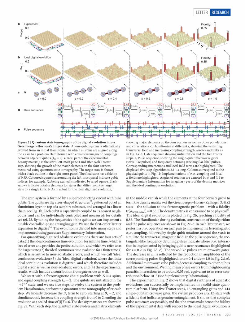
We start with a ferromagnetic chain problem with N = 4 spins, and equal coupling strength Jzz = 2. The qubits are initialized in the | + ⟩ ⊗N state, and we use five steps to evolve the system to the prob-lem Hamiltonian, performing quantum state tomography after each step. We linearly decrease the Bx term to zero, starting at Bx = 2, and simultaneously increase the coupling strength from 0 to 2, ending the evolution at a scaled time of | J| T = 6. The density matrices are shown in Fig. 2a. With each step, the quantum state evolves and matrix elements

in the middle vanish while the elements at the four corners grow to form the density matrix ρ of the Greenberger–Horne–Zeilinger (GHZ) state—the solution to the ferromagnetic problem—with a fidelity tr(ρtarget-stateρ) = 0.55. The density matrix is constrained to be physical25. The ideal digital evolution is plotted in Fig. 2b, reaching a fidelity of 0.85. The Hamiltonian during evolution, construction of the algorithm and the pulse sequence are shown in Fig. 2c–e. In each Trotter step, we perform a σzσz operation on each pair to implement the ferromagnetic σzσz coupling, followed by single-qubit rotations around the x axis to simulate the transversal magnetic field. In the pulse sequence, the rec-tangular-like frequency detuning pulses indicate where σzσz interac-tion is implemented by bringing qubits near resonance (highlighted for s = 0.2 in Fig. 2d, e). The wave-like pulses are microwave gates. The decrease in Bx is reflected by the reduction in amplitudes of the corresponding pulses (highlighted for s = 0.4 and s = 1.0 in Fig. 2d, e). Additional microwave echo pulses decrease coupling to other qubits and the environment. We find mean phase errors from neighbouring parasitic interactions to be around 0.05 rad, equivalent to an error con-tribution below 10−3 (see Supplementary Information).

The experiment in Fig. 2 shows that digital synthesis of adiabatic evolutions can successfully be implemented in a solid-state quan-tum platform. Using five Trotter steps, 15 entangling gates and 144 single-qubit microwave gates, the system produces a GHZ state with a fidelity that indicates genuine entanglement. It shows that complex pulse sequences are possible, and that the errors make sense: the fidelity of the experimental data with respect to the ideal digital evolution is

X

X

X

X

X

X

X

X

X

X

X

X

X

X

X

X

X

X

X

X

z z2

z z2

z z2

z z2

z z2

z z2

z z2

z z2

z z2

z z2

z z2

z z2

z z2

z z2

z z2

|+⟩

|+⟩

|+⟩

|+⟩

0.5

0.0

Fidelity: 0.55

s = 0.0 s = 0.2 s = 0.4 s = 0.6 s = 0.8 s = 1.0

Experiment

Ideal digital evolution

Gate sequence

Pulse sequence

Fidelity: 0.85

a

b

d

e

0.5

0.0

c H

2,3Jzz 3Bx

2Bx

0Bx1Bx

Re(

)R

e()

Figure 2 | Quantum state tomography of the digital evolution into a Greenberger–Horne–Zeilinger state. A four-qubit system is adiabatically evolved from an initial Hamiltonian in which all spins are aligned along the x axis to a problem Hamiltonian with equal ferromagnetic couplings between adjacent qubits (Jzz = 2). a, Real part of the experimental density matrix ρ at the start (left-most panel) and after each Trotter step, showing the growth of the major elements on the four corners, measured using quantum state tomography. The target state is shown with a black outline in the right-most panel. The final state has a fidelity of 0.55. Coloured squares surrounding the left-most panel indicate qubit indices: for example, Q0 being excited is indicated by a red square. Black arrows indicate notable elements for states that differ from the target state by a single kink. b, As in a, but for the ideal digitized evolution,

showing major elements on the four corners as well as other populations and correlations. c, Hamiltonian at different s, showing the vanishing transversal field and increasing coupling strength; arrows and links as in Fig. 1a. d, Gate sequence showing initialization and the five Trotter steps. e, Pulse sequence, showing the single-qubit microwave gates (wave-like pulses) and frequency detuning (rectangular-like) pulses. Corresponding interactions and local field terms are highlighted. The displayed five-step algorithm is 2.1-μ s long. Colours correspond to the physical qubits in Fig. 1b. Implementations of σzσz coupling and local x-fields are highlighted. Angles of rotation are denoted by φ and θ. See Supplementary Information for imaginary parts of the density matrices and the ideal continuous evolution.

© 2016 Macmillan Publishers Limited. All rights reserved

LETTERRESEARCH

2 2 4 | N A T U R E | V O L 5 3 4 | 9 J U N E 2 0 1 6

0.64. The overlap between the ideal digital evolution and ideal contin-uous time evolution for finite time is 0.93, and the overlap of this con-tinuous evolution with the GHZ state (see Supplementary Information) is 0.88. The product of the above three values (0.52) is close to the experimental fidelity of 0.55, and shows that the experimental error is a combination of non-adiabatic, digitization and gate errors. Adopting the entangling gate error of 7.4 × 10−3 and 8 × 10−4 as measured in ref. 25, we expect an accumulated gate error of 0.23 whereas we find an infidelity of 0.36; we attribute the difference to errors in maintaining the phases of the four-qubit system for a duration of 2.1 μ s.

An important feature of the errors is the prevalence of populations and correlations of the | 0001⟩ , | 0011⟩ and | 0111⟩ states and their bit-wise inverses; see arrows in Fig. 2a. Their elements are also present in the ideal digital results and in the ideal continuous evolutions (see Supplementary Information). These are states that deviate by a single kink from the target state, having a residual energy of 2| J| , indicating the presence of non-adiabatic errors. These kink errors are connected to the formation of defects during a phase transition, as described by the Kibble–Zurek mechanism26,27.

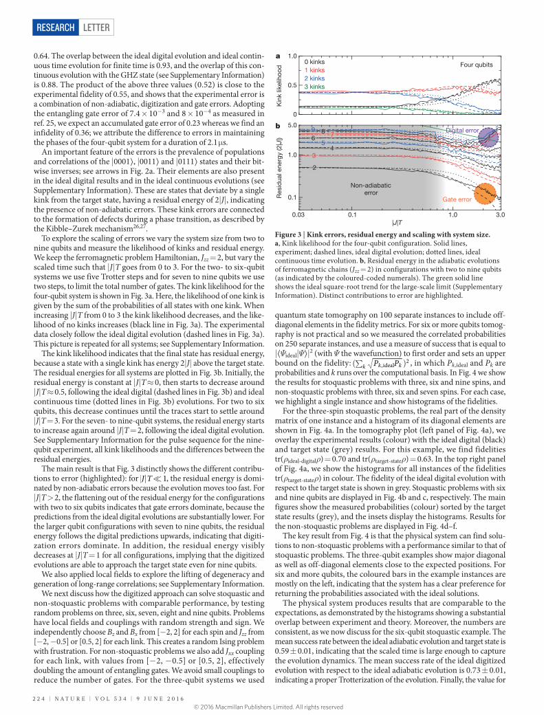
To explore the scaling of errors we vary the system size from two to nine qubits and measure the likelihood of kinks and residual energy. We keep the ferromagnetic problem Hamiltonian, Jzz = 2, but vary the scaled time such that | J| T goes from 0 to 3. For the two- to six-qubit systems we use five Trotter steps and for seven to nine qubits we use two steps, to limit the total number of gates. The kink likelihood for the four-qubit system is shown in Fig. 3a. Here, the likelihood of one kink is given by the sum of the probabilities of all states with one kink. When increasing | J| T from 0 to 3 the kink likelihood decreases, and the like-lihood of no kinks increases (black line in Fig. 3a). The experimental data closely follow the ideal digital evolution (dashed lines in Fig. 3a). This picture is repeated for all systems; see Supplementary Information.

The kink likelihood indicates that the final state has residual energy, because a state with a single kink has energy 2| J| above the target state. The residual energies for all systems are plotted in Fig. 3b. Initially, the residual energy is constant at | J| T ≈ 0, then starts to decrease around | J| T ≈ 0.5, following the ideal digital (dashed lines in Fig. 3b) and ideal continuous time (dotted lines in Fig. 3b) evolutions. For two to six qubits, this decrease continues until the traces start to settle around | J| T = 3. For the seven- to nine-qubit systems, the residual energy starts to increase again around | J| T = 2, following the ideal digital evolution. See Supplementary Information for the pulse sequence for the nine-qubit experiment, all kink likelihoods and the differences between the residual energies.

The main result is that Fig. 3 distinctly shows the different contribu-tions to error (highlighted): for | | �J T 1, the residual energy is domi-nated by non-adiabatic errors because the evolution moves too fast. For | J| T > 2, the flattening out of the residual energy for the configurations with two to six qubits indicates that gate errors dominate, because the predictions from the ideal digital evolutions are substantially lower. For the larger qubit configurations with seven to nine qubits, the residual energy follows the digital predictions upwards, indicating that digiti-zation errors dominate. In addition, the residual energy visibly decreases at | J| T = 1 for all configurations, implying that the digitized evolutions are able to approach the target state even for nine qubits.

We also applied local fields to explore the lifting of degeneracy and generation of long-range correlations; see Supplementary Information.

We next discuss how the digitized approach can solve stoquastic and non-stoquastic problems with comparable performance, by testing random problems on three, six, seven, eight and nine qubits. Problems have local fields and couplings with random strength and sign. We independently choose Bz and Bx from [− 2, 2] for each spin and Jzz from [− 2, − 0.5] or [0.5, 2] for each link. This creates a random Ising problem with frustration. For non-stoquastic problems we also add Jxx coupling for each link, with values from [− 2, − 0.5] or [0.5, 2], effectively doubling the amount of entangling gates. We avoid small couplings to reduce the number of gates. For the three-qubit systems we used

quantum state tomography on 100 separate instances to include off- diagonal elements in the fidelity metrics. For six or more qubits tomog-raphy is not practical and so we measured the correlated probabilities on 250 separate instances, and use a measure of success that is equal to | ⟨ Ψideal| Ψ⟩ | 2 (with Ψ the wavefunction) to first order and sets an upper bound on the fidelity: (∑ )P Pk k k,ideal

2 , in which Pk,ideal and Pk are probabilities and k runs over the computational basis. In Fig. 4 we show the results for stoquastic problems with three, six and nine spins, and non-stoquastic problems with three, six and seven spins. For each case, we highlight a single instance and show histograms of the fidelities.

For the three-spin stoquastic problems, the real part of the density matrix of one instance and a histogram of its diagonal elements are shown in Fig. 4a. In the tomography plot (left panel of Fig. 4a), we overlay the experimental results (colour) with the ideal digital (black) and target state (grey) results. For this example, we find fidelities tr(ρideal-digitalρ) = 0.70 and tr(ρtarget-stateρ) = 0.63. In the top right panel of Fig. 4a, we show the histograms for all instances of the fidelities tr(ρtarget-stateρ) in colour. The fidelity of the ideal digital evolution with respect to the target state is shown in grey. Stoquastic problems with six and nine qubits are displayed in Fig. 4b and c, respectively. The main figures show the measured probabilities (colour) sorted by the target state results (grey), and the insets display the histograms. Results for the non-stoquastic problems are displayed in Fig. 4d–f.

The key result from Fig. 4 is that the physical system can find solu-tions to non-stoquastic problems with a performance similar to that of stoquastic problems. The three-qubit examples show major diagonal as well as off-diagonal elements close to the expected positions. For six and more qubits, the coloured bars in the example instances are mostly on the left, indicating that the system has a clear preference for returning the probabilities associated with the ideal solutions.

The physical system produces results that are comparable to the expectations, as demonstrated by the histograms showing a substantial overlap between experiment and theory. Moreover, the numbers are consistent, as we now discuss for the six-qubit stoquastic example. The mean success rate between the ideal adiabatic evolution and target state is 0.59 ± 0.01, indicating that the scaled time is large enough to capture the evolution dynamics. The mean success rate of the ideal digitized evolution with respect to the ideal adiabatic evolution is 0.73 ± 0.01, indicating a proper Trotterization of the evolution. Finally, the value for

0

1.0

|J|T1.00.1

Res

idua

l ene

rgy

(2|J

|)

1.0

Kin

k lik

elih

ood Four qubits

0.1

3.00.03

Non-adiabaticerror

Gate error

2

34

56 789

0 kinks1 kinks2 kinks3 kinks

a

b

0.5

5.0Digital error

Figure 3 | Kink errors, residual energy and scaling with system size. a, Kink likelihood for the four-qubit configuration. Solid lines, experiment; dashed lines, ideal digital evolution; dotted lines, ideal continuous time evolution. b, Residual energy in the adiabatic evolutions of ferromagnetic chains (Jzz = 2) in configurations with two to nine qubits (as indicated by the coloured-coded numerals). The green solid line shows the ideal square-root trend for the large-scale limit (Supplementary Information). Distinct contributions to error are highlighted.

© 2016 Macmillan Publishers Limited. All rights reserved

LETTER RESEARCH

9 J U N E 2 0 1 6 | V O L 5 3 4 | N A T U R E | 2 2 5

the experimental evolution with respect to the ideal digitized evolution is 0.714 ± 0.006, indicating that the experiment follows the ideal digital evolution reasonably well. The product of these three numbers, 0.31, is very close to the mean value between the experimental data and the target state, 0.296 ± 0.007. This shows that the experimental errors arise from comparable contributions of non-adiabatic, digital and gate errors. For the six-qubit non-stoquastic case, experimental-to-target state values are higher than this product, suggesting that errors par-tially cancel. A further reason for the higher success rate could be that the presence of σxσx terms is helpful for difficult problems in general16. This experiment took up to nine qubits and up to 103 gates. See Supplementary Information for pulse sequences, gate counts, problem parameters and additional metrics.

To further quantify the performance of the system, we compare experimental and random probabilities with the theoretical results. In essence, we take a uniform random distribution over the 2N possible measurement outputs as a baseline sanity check. We find that, for the stoquastic problems, the measures of success of all six- to nine-qubit

configurations are significantly above this baseline: for six qubits, the success measure of the experimental data with respect to the target state is 0.296 ± 0.007, whereas using uniform random probabilities produces a value of 0.168 ± 0.005. For the nine-qubit case the num-bers are 0.122 ± 0.006 for the experimental data and 0.074 ± 0.004 for random. For the non-stoquastic problems the numbers are 0.380 ± 0.009 and 0.335 ± 0.008 for the six-qubit configuration, and 0.311 ± 0.009 and 0.277 ± 0.008 for the seven-qubit configuration. A complete listing for all configurations is provided in Supplementary Information.

This experiment shows that digital synthesis of the adiabatic evo-lutions can be used to find signatures of the ground states of random stoquastic and non-stoquastic problems. Errors arise from a compara-ble contribution of non-adiabatic, digital and gate errors, and success rates are significantly above a uniform random baseline. For larger qubit systems, the number of Trotter steps needs to be limited to reduce the accumulation of gate error, in turn limiting the evolution we can simulate. Therefore, the experimental error is larger, arising from a

Figure 4 | Digital evolutions of random stoquastic and non-stoquastic problems. As stoquastic problems we use frustrated Ising Hamiltonians, with random local x and z fields, and random σzσz couplings. a–c, Stoquastic results for three, six and nine qubits. a, For three qubits we have done tomography. An example instance is provided on the left, where we show the real part of the density matrix ρ. Coloured bars denote the experimental data, and black and grey outlined bars show the ideal digital evolution and the target state, respectively. The diagonals of the experiment (colour) and the target state (grey) are shown in the bottom right panel (as indicated by the dashed arrow), sorted by ideal target state results. The fidelity results for all 100 instances are summarized in the histogram (top right), where ratio denotes the normalized occurrence; coloured bars, fidelities of experimental results with respect to the target

state; grey bars, fidelities of the ideal digital evolution with respect to the target state. b, c, The correlated probabilities for six (b) and nine (c) qubits, sorted by target state results. Experimental data are in colour, the target state is in grey. The results for all 250 instances are summarized in the insets. For the nine-qubit instance (c), the first 100 elements are shown. In a–c, the coloured squares surrounding or below the plots indicate qubit indices, as in Fig. 2. d–f, As in a–c, but for non-stoquastic problems, which have additional random σxσx couplings. Here we plot the data for three, six and seven qubits, for which the average measure of success is above the random baseline (not shown; see text). The results show that the system can find the ground states of stoquastic and non-stoquastic Hamiltonians with similar performance.

Pro

bab

ility

10–1

10–2

Pro

bab

ility

10–1

10–2

Non-stoquastic

Six qubits Six qubits

Nine qubits Seven qubitsP

rob

abili

ty

10–1

10–2

Pro

bab

ility

10–1

10–2

Three qubits

b

c

e

a d

0

0.75

0 1.0Measure of success

0

0.75

0 1.0Measure of success

Stoquastic

Three qubits

0

0.75

0 1Fidelity

10–2

100

Pro

bab

ility

0 1Fidelity0

0.75

10–2

100

Pro

bab

ility

0

0.5

f

0

0.5

Target state

Experiment

0.50.5

Rat

io

Rat

ioR

atio

0

0.75

0 1.0Measure of success

0.5

Rat

io

Rat

io

0

0.75

0 1.0Measure of success

0.5

Rat

io

Re (

)

Re(

)

© 2016 Macmillan Publishers Limited. All rights reserved

LETTERRESEARCH

2 2 6 | N A T U R E | V O L 5 3 4 | 9 J U N E 2 0 1 6

combination of gate, digitization and non-adiabatic error. However, in an error-corrected system, the number of gates is in principle uncon-strained, digitization can be made arbitrarily accurate and one can move more slowly through critical parts of the evolution. Although we have used Trotterization28, the scaling of the digitization becomes more appealing with recent methods based on the truncation of Taylor series29. See Supplementary Information for further motivations and discussions.

We believe that the digitized approach to adiabatic quantum evo-lutions of complex problems—where local fields, variable coupling strengths and types, and multibody interactions can be constructed—would become viable on the small scale with lower gate errors, and that large-scale applications could be achieved in conjunction with error correction. We hope our work accelerates further improvements in superconducting quantum systems and motivates research into the encoding and measurement of non-stoquastic computational problems. In addition, we anticipate that these results encourage work on the effi-cient digitization of algorithms for small- and large-scale systems, for which reducing the effects of noise by, for example, dynamical decou-pling techniques, or reducing the circuit complexity is paramount.

Received 13 November 2015; accepted 1 March 2016.

1. Feynman, R. P. Simulating physics with computers. Int. J. Theor. Phys. 21, 467–488 (1982).

2. Aspuru-Guzik, A., Dutoi, A. D., Love, P. J. & Head-Gordon, M. Simulated quantum computation of molecular energies. Science 309, 1704–1707 (2005).

3. Farhi, E., Goldstone, J., Gutmann, S. & Sipser, M. Quantum computation by adiabatic evolution. Preprint at http://arxiv.org/abs/quant-ph/0001106 (2000).

4. Farhi, E. et al. A quantum adiabatic evolution algorithm applied to random instances of an NP-complete problem. Science 292, 472–475 (2001).

5. Nishimori, H. Statistical Physics of Spin Glasses and Information Processing: An Introduction (Oxford Univ. Press, 2001).

6. Lloyd, S. Universal quantum simulators. Science 273, 1073–1078 (1996).7. Bravyi, S. B. & Kitaev, A. Yu. Quantum codes on a lattice with boundary.

Preprint at http://arxiv.org/abs/quant-ph/9811052 (1998).8. Fowler, A. G., Mariantoni, M., Martinis, J. M. & Cleland, A. N. Surface codes:

towards practical large-scale quantum computation. Phys. Rev. A 86, 032324 (2012).

9. Steffen, M. et al. Experimental implementation of an adiabatic quantum optimization algorithm. Phys. Rev. Lett. 90, 067903 (2003).

10. Lanyon, B. P. et al. Universal digital quantum simulation with trapped ions. Science 334, 57–61 (2011).

11. Barends, R. et al. Digital quantum simulation of fermionic models with a superconducting circuit. Nat. Commun. 6, 7654 (2015).

12. Salathé, Y. et al. Digital quantum simulation of spin models with circuit quantum electrodynamics. Phys. Rev. X 5, 021027 (2015).

13. Bravyi, S., DiVincenzo, D. P., Oliveira, R. I. & Terhal, B. M. The complexity of stoquastic local Hamiltonian problems. Quantum Inf. Comput. 8, 361–385 (2008).

14. Aharonov, D. et al. Adiabatic quantum computation is equivalent to standard quantum computation. SIAM Rev. 50, 755–787 (2008).

15. Lloyd, S. & Terhal, B. M. Adiabatic and Hamiltonian computing on a 2D lattice with simple two-qubit interactions. New J. Phys. 18, 023042 (2016).

16. Crosson, E., Farhi, E., Lin, C. Y.-Y., Lin, H.-H. & Shor, P. Different strategies for optimization using the quantum adiabatic algorithm. Preprint at http://arxiv.org/abs/1401.7320 (2014).

17. Babbush, R., Love, P. J. & Aspuru-Guzik, A. Adiabatic quantum simulation of quantum chemistry. Sci. Rep. 4, 6603 (2014).

18. Troyer, M. & Wiese, U.-J. Computational complexity and fundamental limitations to fermionic quantum Monte Carlo simulations. Phys. Rev. Lett. 94, 170201 (2005).

19. Boixo, S. et al. Computational multiqubit tunnelling in programmable quantum annealers. Nat. Commun. 7, 10327 (2016).

20. Bravyi, S. B. & Kitaev, A. Yu. Fermionic quantum computation. Ann. Phys. 298, 210–226 (2002).

21. Seeley, J. T., Richard, M. J. & Love, P. J. The Bravyi–Kitaev transformation for quantum computation of electronic structure. J. Chem. Phys. 137, 224109 (2012).

22. Barends, R. et al. Coherent Josephson qubit suitable for scalable quantum integrated circuits. Phys. Rev. Lett. 111, 080502 (2013).

23. Kelly, J. et al. State preservation by repetitive error detection in a superconducting quantum circuit. Nature 519, 66–69 (2015).

24. Suzuki, M. Fractal decomposition of exponential operators with applications to many-body theories and Monte Carlo simulations. Phys. Lett. A 146, 319–323 (1990).

25. Barends, R. et al. Superconducting quantum circuits at the surface code threshold for fault tolerance. Nature 508, 500–503 (2014).

26. Kibble, T. W. B. Some implications of a cosmological phase transition. Phys. Rep. 67, 183–199 (1980).

27. Zurek, W. H. Cosmological experiments in superfluid helium? Nature 317, 505–508 (1985).

28. Wiebe, N., Berry, D., Hoyer, P. & Sanders, B. C. Higher order decompositions of ordered operator exponentials. J. Phys. A 43, 065203 (2010).

29. Berry, D., Childs, A. M., Cleve, R., Kothari, R. & Somma, R. D. Simulating Hamiltonian dynamics with a truncated Taylor series. Phys. Rev. Lett. 114, 090502 (2015).

Supplementary Information is available in the online version of the paper.

Acknowledgements We acknowledge support from Spanish MINECO FIS2012-36673-C03-02; Ramón y Cajal grant RYC-2012-11391; UPV/EHU UFI 11/55 and EHUA14/04; Basque Government IT472-10; a UPV/EHU PhD grant; and PROMISCE and SCALEQIT EU projects. Devices were made at the UC Santa Barbara Nanofabrication Facility, a part of the NSF-funded National Nanotechnology Infrastructure Network, and at the NanoStructures Cleanroom Facility.

Author Contributions R. Barends, A.S. and L.L. designed the experiment, with E.S., H.N. and J.M.M. providing supervision and A. Mezzacapo, U.L.H. and R. Babbush providing additional theoretical support. R. Barends, A.S., L.L. and R. Babbush co-wrote the manuscript with E.S., H.N. and J.M.M. R. Barends, A.S. and L.L. performed the experiment and analysed the data. The device was designed by R. Barends and J.K. All authors contributed to the fabrication process, experimental set-up and manuscript preparation.

Author Information Reprints and permissions information is available at www.nature.com/reprints. The authors declare no competing financial interests. Readers are welcome to comment on the online version of the paper. Correspondence and requests for materials should be addressed to R. Barends (barends@google.com) or A.S. (shabani@google.com).

© 2016 Macmillan Publishers Limited. All rights reserved