Embed Size (px)
Citation preview

Digital Signal Processing for Medical ImagingUsing Matlab

E. S. Gopi
Digital Signal Processingfor Medical Imaging UsingMatlab
123

E. S. GopiDepartment of Electronics
and Communications EngineeringNational Institute of Technology TrichyTiruchirappalli, Tamil NaduIndia
ISBN 978-1-4614-3139-8 ISBN 978-1-4614-3140-4 (eBook)DOI 10.1007/978-1-4614-3140-4Springer New York Heidelberg Dordrecht London
Library of Congress Control Number: 2012944390
� Springer Science+Business Media New York 2013This work is subject to copyright. All rights are reserved by the Publisher, whether the whole or part ofthe material is concerned, specifically the rights of translation, reprinting, reuse of illustrations,recitation, broadcasting, reproduction on microfilms or in any other physical way, and transmission orinformation storage and retrieval, electronic adaptation, computer software, or by similar or dissimilarmethodology now known or hereafter developed. Exempted from this legal reservation are briefexcerpts in connection with reviews or scholarly analysis or material supplied specifically for thepurpose of being entered and executed on a computer system, for exclusive use by the purchaser of thework. Duplication of this publication or parts thereof is permitted only under the provisions ofthe Copyright Law of the Publisher’s location, in its current version, and permission for use must alwaysbe obtained from Springer. Permissions for use may be obtained through RightsLink at the CopyrightClearance Center. Violations are liable to prosecution under the respective Copyright Law.The use of general descriptive names, registered names, trademarks, service marks, etc. in thispublication does not imply, even in the absence of a specific statement, that such names are exemptfrom the relevant protective laws and regulations and therefore free for general use.While the advice and information in this book are believed to be true and accurate at the date ofpublication, neither the authors nor the editors nor the publisher can accept any legal responsibility forany errors or omissions that may be made. The publisher makes no warranty, express or implied, withrespect to the material contained herein.
Printed on acid-free paper
Springer is part of Springer Science+Business Media (www.springer.com)

Dedicated to my wife G. Viji, son A. G. Vasigand daughter A. G. Desna
Preface
Digital signal processing (DSP) techniques, like Radon transformation, Projectiontechniques, Fourier transformation in polar form, Hankel transformation, etc., areused in Medical imaging techniques like Computed Tomography (CT) andMagnetic Resonance Imaging (MRI) during the process of imaging. These are notusually covered in the regular DSP and Image processing books. This book iswritten with the intention to focus the DSP aspects used during the process ofimaging in CT and MRI. Also, DSP aspects used in the post imaging techniquessuch as Image enhancement, Image compression and pattern recognition are alsodiscussed in this book. The Matlab illustrations are given for better understanding.This book is suitable for beginners who are doing research in Medical imagingprocessing.
vii

Acknowledgments
I am very much thankful to Prof. P. Palanisamy, Department of ECE, NationalInstitute of Technology, Trichy, for his encouragement. I am extremely happy toexpress my thanks to Prof. K. M. M. Prabhu (IITM), Prof. M. Chidambaram(IITM), Prof. S. Sundararajan (NITT), Prof. P. Somaskandan (NITT), Prof. B.Venkataramani (NITT), and Prof. S. Raghavan (NITT) for their support. I alsothank those who were directly or indirectly involved in bringing up this booksuccessfully. Special thanks to my parents Mr. E. Sankara Subbu and Mrs. E. S.Meena.
ix

Contents
1 Radon Transformation . . . . . . . . . . . . . . . . . . . . . . . . . . . . . . . . . 11.1 Introduction to Computed Tomography (CT) . . . . . . . . . . . . . . 11.2 Parallel Beam Projection . . . . . . . . . . . . . . . . . . . . . . . . . . . . 1
1.2.1 Discrete Realization of (1.15) . . . . . . . . . . . . . . . . . . . . 51.2.2 List of Figs. 1.1 to 1.11 in Terms of the
Notations Used . . . . . . . . . . . . . . . . . . . . . . . . . . . . . . 61.3 Fanbeam Projection . . . . . . . . . . . . . . . . . . . . . . . . . . . . . . . . 9
1.3.1 Relationship Between Parallel Beamand Fanbeam Projection. . . . . . . . . . . . . . . . . . . . . . . . 10
1.3.2 Discrete Realization of (1.25) . . . . . . . . . . . . . . . . . . . . 151.3.3 List of Figs. 1.12 to 1.25 in Terms
of the Notations used. . . . . . . . . . . . . . . . . . . . . . . . . . 17
2 Magnetic Resonance Imaging . . . . . . . . . . . . . . . . . . . . . . . . . . . . 272.1 Bloch Equation . . . . . . . . . . . . . . . . . . . . . . . . . . . . . . . . . . . 272.2 Comment on the Equations (2.8)–(2.10) . . . . . . . . . . . . . . . . . . 292.3 The Larmor Frequency and the Tip Angle a . . . . . . . . . . . . . . . 29
2.3.1 Disturbance to Obtain Non-Zero a Value. . . . . . . . . . . . 302.3.2 Observation on (2.22) and (2.25) . . . . . . . . . . . . . . . . . 33
2.4 Trick on MRI . . . . . . . . . . . . . . . . . . . . . . . . . . . . . . . . . . . . 352.5 Selecting the Human Slice and the Corresponding
External RF Pulse . . . . . . . . . . . . . . . . . . . . . . . . . . . . . . . . . 352.5.1 Summary of the Section 2.5 . . . . . . . . . . . . . . . . . . . . . 38
2.6 Measurement of the Transverse Component Usingthe Receiver Antenna. . . . . . . . . . . . . . . . . . . . . . . . . . . . . . . 392.6.1 Observation on (2.47)–(2.50) . . . . . . . . . . . . . . . . . . . . 402.6.2 Receiver to Receive the Transverse Component . . . . . . . 40
2.7 Sampling the MRI Image in the Frequency Domain . . . . . . . . . 41
xi

2.8 Practical Difficulties and Remedies in MRI . . . . . . . . . . . . . . . 422.8.1 Proton-Density MRI Image Using Gradient Echo . . . . . . 432.8.2 T2 MRI Image Using Spin–Echo and
Carteisian Scanning. . . . . . . . . . . . . . . . . . . . . . . . . . . 442.8.3 T2 MRI Image Using Spin–Echo and
Polar Scanning . . . . . . . . . . . . . . . . . . . . . . . . . . . . . . 462.8.4 T1 MRI Image . . . . . . . . . . . . . . . . . . . . . . . . . . . . . . 47
3 Illustrations on MRI Techniques Using Matlab . . . . . . . . . . . . . . . 493.1 Illustration on the Steps Involved in Obtaining
Proton-Density MRI Image . . . . . . . . . . . . . . . . . . . . . . . . . . . 493.1.1 Proton-Density MRI Imaging . . . . . . . . . . . . . . . . . . . . 50
3.2 Illustration on the Steps Involved in Obtainingthe T2 MRI Image Using Cartesian Scanning . . . . . . . . . . . . . . 533.2.1 Note to the Fig. 3.4 . . . . . . . . . . . . . . . . . . . . . . . . . . . 573.2.2 Momentary Peak Due to Spin Echo . . . . . . . . . . . . . . . 60
3.3 Illustration on the Steps Involved in Obtainingthe T2 MRI Image Using Polar Scanning . . . . . . . . . . . . . . . . . 633.3.1 Reconstructing f ðx; yÞ from Gðr; hÞ . . . . . . . . . . . . . . . . 64
3.4 Illustration on the Steps Involved in Obtainingthe T1 MRI Image . . . . . . . . . . . . . . . . . . . . . . . . . . . . . . . . . 683.4.1 t1.m . . . . . . . . . . . . . . . . . . . . . . . . . . . . . . . . . . . . . 70
4 Medical Image Processing . . . . . . . . . . . . . . . . . . . . . . . . . . . . . . 734.1 Summary on the Various Medical Imaging Techniques . . . . . . . 734.2 Image Enhancement. . . . . . . . . . . . . . . . . . . . . . . . . . . . . . . . 74
4.2.1 Logirthmic Display . . . . . . . . . . . . . . . . . . . . . . . . . . . 744.2.2 Non-Linear Filtering . . . . . . . . . . . . . . . . . . . . . . . . . . 744.2.3 Image Substraction . . . . . . . . . . . . . . . . . . . . . . . . . . . 744.2.4 Linear Filterering and the Hankel Transformation . . . . . . 764.2.5 Histogram Equalization . . . . . . . . . . . . . . . . . . . . . . . . 804.2.6 Histogram Specification . . . . . . . . . . . . . . . . . . . . . . . . 81
4.3 Image Compression . . . . . . . . . . . . . . . . . . . . . . . . . . . . . . . . 824.3.1 Discrete Cosine Transformation (DCT) . . . . . . . . . . . . . 824.3.2 Using KL-Transformation . . . . . . . . . . . . . . . . . . . . . . 85
4.4 Feature Extraction and Classification . . . . . . . . . . . . . . . . . . . . 864.4.1 Using Discrete Wavelet Transformation. . . . . . . . . . . . . 874.4.2 Dimensionality Reduction Using Principal Component
Analysis (PCA). . . . . . . . . . . . . . . . . . . . . . . . . . . . . . 894.4.3 Dimensionality Reduction Using Linear Discriminant
Analysis (LDA) . . . . . . . . . . . . . . . . . . . . . . . . . . . . . 934.4.4 Dimensionality Reduction Using Kernel-Linear
Discriminant Analysis (K-LDA) . . . . . . . . . . . . . . . . . . 96
xii Contents

Appendix A: Solving Bloch Equation with ADv sincðDvtÞ Envelope . . . 101
Appendix B: Projection Techniques . . . . . . . . . . . . . . . . . . . . . . . . . . 103
Appendix C: Hankel Transformation . . . . . . . . . . . . . . . . . . . . . . . . . 107
Appendix D: List of m-Files. . . . . . . . . . . . . . . . . . . . . . . . . . . . . . . . 109
Index . . . . . . . . . . . . . . . . . . . . . . . . . . . . . . . . . . . . . . . . . . . . . . . . 111
Contents xiii

Chapter 1Radon Transformation
1.1 Introduction to Computed Tomography (CT)
The physical setup to obtain the CT of the particular slice of the test body involvespassing the X-ray to that particular slice and detecting the attenuated signal at theother side. This value is conceptually proportional to the integral value of sliced imagealong the X-ray paths. The ray-path directions with respect to sliced image describesthe type of projection used in that CT. There are two major types of projectiontechniques namely Parallel beam projection and Fan-beam projection used in CT.The process of reconstructing the image from the projected data involves digitalsignal processing, which are described below.
1.2 Parallel Beam Projection
Let us consider an example image (refer Fig. 1.1) as the sliced image of the testbody. The parallel beam projection involves transmitting X-ray signals one after andanother, parallel to each other and the corresponding attenuated signals are capturedusing the detector kept exactly on the other sides of the ray (refer Fig. 1.2). This isequivalent to obtaining the line integration of the image in the direction of the parallelbeam. This is the radon transformation with an angle 0◦. Now the image is rotatedin the clock-wise direction with an angle θ◦ and the line integration is computedas mentioned above. This is the radon transformation with angle θ◦. (In practice,this is obtained by shifting the positions of the source and the detector such thatthe imaginary line joining the source and the detector is rotated in the anticlockwisedirection by an angle θ◦). This is repeated for the angle θ◦ ranging from 0 to 360◦.This completes the forward radon transformation. The process of estimating theoriginal image from the forward radon transformation data is called as inverse radontransformation, which is described below.
E. S. Gopi, Digital Signal Processing for Medical Imaging Using Matlab, 1DOI: 10.1007/978-1-4614-3140-4_1, © Springer Science+Business Media New York 2013
2 1 Radon Transformation
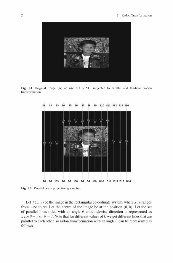
Fig. 1.1 Original image (A) of size 511 × 511 subjected to parallel and fan-beam radontransformation
Fig. 1.2 Parallel beam projection geometry
Let f (x, y) be the image in the rectangular co-ordinate system, where x, y rangesfrom −∞ to ∞. Let the centre of the image be at the position (0, 0). Let the setof parallel lines titled with an angle θ anticlockwise direction is represented asx cos θ + y sin θ = l. Note that for different values of l, we get different lines that areparallel to each other. so radon transformation with an angle θ can be represented asfollows.

1.2 Parallel Beam Projection 3
R(l, θ) =∞∫
−∞
∞∫
−∞f (x, y)δ(x cos θ + y sin θ − l)dxdy (1.1)
For the fixed θ, R(l, θ) = R(l). Taking fourier transformation of R(l), we getthe following.
G(U ) =∞∫
−∞R(l) exp− j2πUldl (1.2)
⇒ G(U ) =∞∫
−∞
∞∫
−∞
∞∫
−∞f (x, y)δ(x cos θ + y sin θ − l)dxdy exp− j2πUl dl (1.3)
⇒ G(U ) =∞∫
−∞
∞∫
−∞f (x, y) exp− j2π(x cos θ+y sin θ)U dxdy (1.4)
Let the 2D-Fourier transformation of the image matrix f (x, y) be represented asF(U ′, V ′). It is noted from the (1.4) that G(U ) = F(U ′, V ′), when U ′ = U cos θ
and V ′ = U sin θ . If the values are collected from the 2D-Fourier transformationF(U ′, V ′) of f(x,y), along the line U ′ cos(θ) + V ′ sin(θ) = U ((i.e) for various U ),we get G(U ). This is called projection-slice theorem.
f (x, y) is obtained from the F(U ′, V ′) using inverse 2D-Fourier transformationas mentioned below.
f (x, y) =∞∫
−∞
∞∫
−∞F(U ′, V ′) exp j2π(xU ′+yV ′) dU ′dV ′ (1.5)
Substituting U ′ = U cos θ and V ′ = U sin θ in (1.5), we get the following.F(U cos θ, V sin θ) = G(U, θ), which is the Fourier transformation of g(l, θ) for theconstant θ (refer (1.2)). Changing the variables from (x, y) to (U, θ), (1.5) becomes
f (x, y) =π∫
−π
∞∫
0
G(U, θ) exp j2π(x cos θ+y sin θ)U |J |dUdθ (1.6)
where |J |, is the jacobian of the transformation U = √U ′2 + V ′2, θ = tan−1 V ′
U ′ .
(i.e) J =[
∂U∂U ′ ∂U
∂V ′∂θ∂U ′ ∂θ
∂V ′
]⇒ |J | = |U |

4 1 Radon Transformation
Hence,(1.6) is rewritten as
f (x, y) =π∫
−π
∞∫
0
G(U, θ) exp j2π(x cos θ+y sin θ)U |U |dUdθ (1.7)
From (1.1), we get R(l, θ) = R(−l, θ + π). This implies
G(−U, θ) = G(U, θ + π) (1.8)
Splitting (1.7) into two terms,I-term:
0∫
−π
∞∫
−∞G(U, θ) exp j2π(x cos θ+y sin θ)U |U |dUdθ (1.9)
II-term:π∫
0
∞∫
0
G(U, θ) exp j2π(x cos θ+y sin θ)U |U |dUdθ (1.10)
Change the variable φ = θ + π and U1 = −U in the first term (1.9), we get
π∫
0
∞∫
0
G(−U1, φ − π) exp j2π(x cos φ+y sin φ)U1 |U1|dU1dφ (1.11)
Using (1.7)–(1.11), we get
f (x, y) = 2
π∫
0
∞∫
0
G(U1, φ − π + π) exp j2π(x cos φ+y sin φ)U1 |U1|dU1dφ.
(1.12)Replacing the dummy variables U1 and φ with U and θ respectively in (1.12)
and writing the second limit ranging from −∞ to ∞, we get the following.
f (x, y) = 2(1/2)
π∫
0
∞∫
−∞G(U, θ) exp j2π(x cos θ+y sin θ)U |U |dUdθ (1.13)
Let l = x cos θ + y sin θ . Thus rewriting (1.12) as follows.
f (x, y) =π∫
0
∞∫
−∞G(U, θ) exp j2πlU |U |dUdθ (1.14)
1.2 Parallel Beam Projection 5
Note that∫ ∞−∞ G(U, θ) exp j2πlU |U |dU is the inverse fourier transformation of
the function G(U, θ)|U | for constant θ . This can be achieved as the convolution ofinverse fourier transform (IFT) of G(U, θ) and IFT of |U |. Note that IFT of G(U, θ)
is R(l, θ) for constant θ (refer (1.2)). Final reconstruction formula from parallel beamradon transformation R(l, θ) is represented as follows.
f (x, y) =π∫
0
R(l, θ) ∗ I FT (|U |)dθ (1.15)
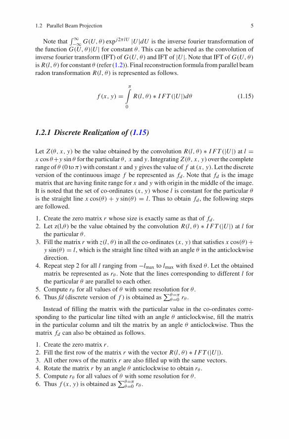
1.2.1 Discrete Realization of (1.15)
Let Z(θ, x, y) be the value obtained by the convolution R(l, θ) ∗ I FT (|U |) at l =x cos θ+y sin θ for the particular θ, x and y. Integrating Z(θ, x, y) over the completerange of θ (0 to π ) with constant x and y gives the value of f at (x, y). Let the discreteversion of the continuous image f be represented as fd . Note that fd is the imagematrix that are having finite range for x and y with origin in the middle of the image.It is noted that the set of co-ordinates (x, y) whose l is constant for the particular θ
is the straight line x cos(θ) + y sin(θ) = l. Thus to obtain fd , the following stepsare followed.
1. Create the zero matrix r whose size is exactly same as that of fd .2. Let z(l,θ ) be the value obtained by the convolution R(l, θ) ∗ I FT (|U |) at l for
the particular θ .3. Fill the matrix r with z(l, θ) in all the co-ordinates (x, y) that satisfies x cos(θ)+
y sin(θ) = l, which is the straight line tilted with an angle θ in the anticlockwisedirection.
4. Repeat step 2 for all l ranging from −lmax to lmax with fixed θ . Let the obtainedmatrix be represented as rθ . Note that the lines corresponding to different l forthe particular θ are parallel to each other.
5. Compute rθ for all values of θ with some resolution for θ .6. Thus fd (discrete version of f ) is obtained as
∑θ=πθ=0 rθ .
Instead of filling the matrix with the particular value in the co-ordinates corre-sponding to the particular line tilted with an angle θ anticlockwise, fill the matrixin the particular column and tilt the matrix by an angle θ anticlockwise. Thus thematrix fd can also be obtained as follows.
1. Create the zero matrix r .2. Fill the first row of the matrix r with the vector R(l, θ) ∗ I FT (|U |).3. All other rows of the matrix r are also filled up with the same vectors.4. Rotate the matrix r by an angle θ anticlockwise to obtain rθ .5. Compute rθ for all values of θ with some resolution for θ .6. Thus f (x, y) is obtained as
∑θ=πθ=0 rθ .

6 1 Radon Transformation
Fig. 1.3 Parallel beam radon transformation of the image ‘A’ (refer Fig. 1.1) with thetaresolution = 0.5014◦
1.2.2 List of Figs. 1.1 to 1.11 in Terms of the Notations Used
• Figure 1.1: Original image subjected to parallel beam projection.• Figure 1.2: Parallel beam projection geometry• Figure 1.3: R(l, θ) (Sinogram) corresponding to the original image with the reso-
lution of θ = 24.5682.• Figure 1.4: Impulse response and the transfer function of the filter |U |• Figure 1.5: R(l, θ) for θ = 24.5682 degree and R(l, θ) ∗ |U |• Figure 1.6: rθ for various θ with R(l, θ) ∗ I FT (|U |) = R(l, θ) ((i.e.) without
filtering)• Figure 1.7: rθ for various θ (with filtering)• Figure 1.8:
∑θ=�θ=0 rθ for various � with R(l, θ) ∗ I FT (|U |) = R(l, θ) ((i.e.)
without filtering)• Figure 1.9:
∑θ=�θ=0 rθ for various � ((i.e.)without filtering)
• Figure 1.10: Final reconstructed image fd obtained with R(l, θ) ∗ I FT (|U |) =R(l, θ) ((i.e) without filtering)
• Figure 1.11: Final reconstructed image fd (with filtering)

1.2 Parallel Beam Projection 7
Fig. 1.4 Impulse response of the ramp filter and the corresponding spectrum
Fig. 1.5 Original and the corresponding filtered parallel beam projection for θ = 24.5682◦
1.2.2.1 Parallelbeamprojection.m
RECONSTRUCTEDIMAGE=0;load VASIGIMAGEC=C(1:1:255,1:1:255);C=[zeros(128,511);zeros(255,128) C zeros(255,128);zeros
(128,511)];B=double(C)/255;T=1;

8 1 Radon Transformation
Fig. 1.6 Illustration of original (without filtering) parallel beam backprojected images obtainedfor θ = 0, 20.0557, 40.1114, 60.1617, 80.2228, 100.2786, 120.3343, 140.3900, 160.4457◦ (Notethat parallel-beam reconstructed images are computed for all θ ranging from 0 to 180◦ with theresolution of 0.5014◦)
angleresolution=360;for theta=0:(180/(angleresolution-1)):180%disp( theta)RADONTRANSFORMATION{T}=sum(imrotate(B,theta,’nearest’,’crop’));T=T+1;end%Back projection technique to get back the dataS=1;Z=[1:10:359];Z=[Z 0];z=1;k=0;for theta=0:(180/(angleresolution-1)):180k=k+1;disp( theta)%Filtering with ramp spectrumtemp=conv(RADONTRANSFORMATION{S},fir2(102,(0:1/101:1),(0:1/101:1),rectwin(103)));
temp=repmat(temp,size(temp,2),1)’;

1.2 Parallel Beam Projection 9
Fig. 1.7 Illustration of filtered parallel beam backprojected images obtained for θ = 0, 20.0557,
40.1114, 60.1617, 80.2228, 100.2786, 120.3343, 140.3900, 160.4457◦ (Note that parallel-beamreconstructed images are computed for all θ ranging from 0 to 180◦ with the resolution of 0.5014◦)
temp=imrotate(temp,90);D=imrotate(temp,-theta,’nearest’,’crop’);RECONSTRUCTEDIMAGE=RECONSTRUCTEDIMAGE+D;if(Z(z)==k)SNAPSHOT_RECONSTRUCTED{z}=RECONSTRUCTEDIMAGE;SNAPSHOP_DATA{z}=D;z=z+1;endS=S+1;endfigurecolormap(gray(256))imagesc(RECONSTRUCTEDIMAGE)

10 1 Radon Transformation
Fig. 1.8 Illustration of reconstruction of the image obtained by cumulative summation of originalparallel beam backprojected images
1.3 Fanbeam Projection
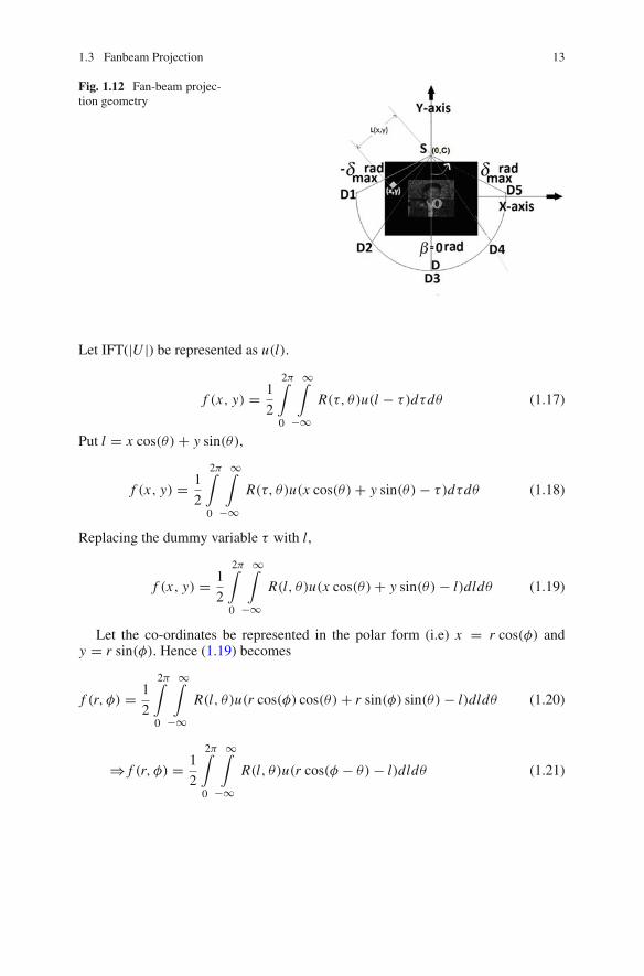
The parallel beam projection technique based CT Scan takes more scanning time.Hence Fanbeam projection technique based CT Scan is used. The Geometry for theFan beam projection is as mentioned in the Fig. 1.12. The single X-ray source (S) keptin the y-axis at the distance D from the origin is subjected to the slice of the test bodyand the multiple detectors (D1–D5 ) kept at the circumference of the sector (obtainedwith S as the centre) are used to capture the attenuated signal along the ray of paths.Mathematically this is proportional to the line integrals taken along the ray of paths.This arrangement helps in reducing the scanning time. This corresponds to the angleβ = 0. Further the source is tilted by an angle β = B in the anticlockwise directionand the corresponding attenuated signals are captured. This is repeated for β rangingfrom 0 to 2π radians. Positions of the detectors are described by the angle measuredfrom reference line segment SD to the line segment joining the source(S) and thedetector in the anticlockwise direction. This angle is represented as δ. Detector 1(refer Fig. 1.12), is kept at an angle −δmax and the detector 5 is kept at an angle+δmax.
1.3 Fanbeam Projection 11
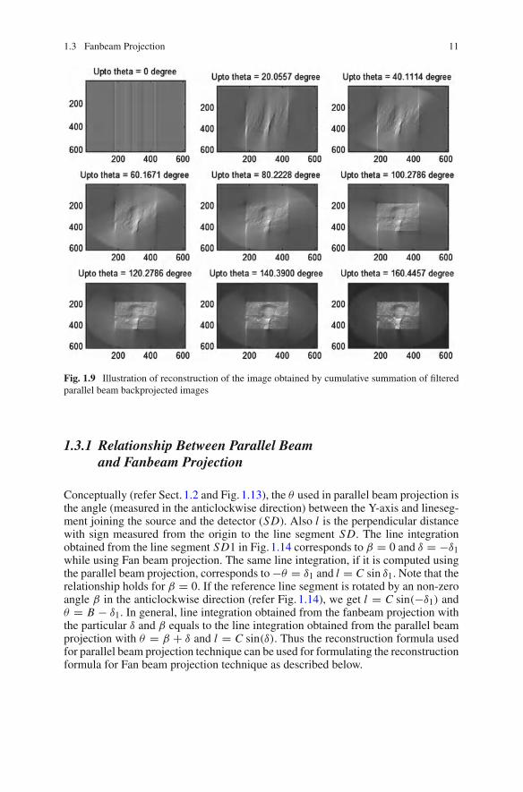
Fig. 1.9 Illustration of reconstruction of the image obtained by cumulative summation of filteredparallel beam backprojected images
1.3.1 Relationship Between Parallel Beamand Fanbeam Projection
Conceptually (refer Sect. 1.2 and Fig. 1.13), the θ used in parallel beam projection isthe angle (measured in the anticlockwise direction) between the Y-axis and lineseg-ment joining the source and the detector (SD). Also l is the perpendicular distancewith sign measured from the origin to the line segment SD. The line integrationobtained from the line segment SD1 in Fig. 1.14 corresponds to β = 0 and δ = −δ1while using Fan beam projection. The same line integration, if it is computed usingthe parallel beam projection, corresponds to −θ = δ1 and l = C sin δ1. Note that therelationship holds for β = 0. If the reference line segment is rotated by an non-zeroangle β in the anticlockwise direction (refer Fig. 1.14), we get l = C sin(−δ1) andθ = B − δ1. In general, line integration obtained from the fanbeam projection withthe particular δ and β equals to the line integration obtained from the parallel beamprojection with θ = β + δ and l = C sin(δ). Thus the reconstruction formula usedfor parallel beam projection technique can be used for formulating the reconstructionformula for Fan beam projection technique as described below.

12 1 Radon Transformation
Fig. 1.10 Final reconstructed image obtained from parallel beam without filtering
Fig. 1.11 Final reconstructed image obtained from filtered parallel beam
Rewriting (1.15) with θ ranging from 0 to 2π , we get the following.
f (x, y) = 1
2
2π∫
0
R(l, θ) ∗ I FT (|U |)dθ (1.16)
1.3 Fanbeam Projection 13
Fig. 1.12 Fan-beam projec-tion geometry
Let IFT(|U |) be represented as u(l).
f (x, y) = 1
2
2π∫
0
∞∫
−∞R(τ, θ)u(l − τ)dτdθ (1.17)
Put l = x cos(θ) + y sin(θ),
f (x, y) = 1
2
2π∫
0
∞∫
−∞R(τ, θ)u(x cos(θ) + y sin(θ) − τ)dτdθ (1.18)
Replacing the dummy variable τ with l,
f (x, y) = 1
2
2π∫
0
∞∫
−∞R(l, θ)u(x cos(θ) + y sin(θ) − l)dldθ (1.19)
Let the co-ordinates be represented in the polar form (i.e) x = r cos(φ) andy = r sin(φ). Hence (1.19) becomes
f (r, φ) = 1
2
2π∫
0
∞∫
−∞R(l, θ)u(r cos(φ) cos(θ) + r sin(φ) sin(θ) − l)dldθ (1.20)
⇒ f (r, φ) = 1
2
2π∫
0
∞∫
−∞R(l, θ)u(r cos(φ − θ) − l)dldθ (1.21)

14 1 Radon Transformation
Fig. 1.13 Relationship between parallel beam and the fan-beam projection geometry-1
(1.21) is rewritten using the new set of variables θ = β + δ and l = C sin(δ).
f (r, φ)
=δmax∫
−δmin
2π+δ∫
0+δ
R(C sin(δ), β − δ)u(r cos(φ − β − δ) − C sin(δ))|J |dβdδ,
(1.22)
where |J |, is the jacobian of the transformation θ = β + δ and l = C sin(δ) (i.e)
J =
⎡⎢⎢⎣
∂β
∂θ
∂β∂δ
∂l
∂θ∂θ∂δ
⎤⎥⎥⎦ ⇒ |J | = |C cos(δ)|
Hence, (1.22) is rewritten as
f (r, φ)
=δmax∫
−δmax
−δ+2π∫
−δ+0
R(C sin(δ), β + δ)u(r cos(φ − β − δ) − C sin(δ))|C cos(δ)|dβdδ (1.23)
With constant δ, R(C sin(δ), β + δ) and u(r cos(φ − β − δ) − C sin(δ)) are theperiodic functions of the variable β with period 2π . Thus the final reconstruction

1.3 Fanbeam Projection 15
Fig. 1.14 Relationship between parallel beam and the fan-beam projection geometry-2
formula for Fanbeam projection is given below.
f (r, φ) =δmax∫
−δmax
2π∫
0
R(C sin(δ), β + δ)u(r cos(φ − β − δ) − C sin(δ))|C cos(δ)|dβdδ
(1.24)
interchanging the order of the limits, we get
f (r, φ) =2π∫
0
δmax∫
−δmax
R(C sin(δ), β + δ)u(r cos(φ − β − δ) − C sin(δ))|C cos(δ)|dδdβ
(1.25)
1.3.2 Discrete Realization of (1.25)
Consider the fan-beam ray path joining the source point S and the arbitrary point Pwith polar co-ordinates (r, φ). Let the distance between the S and P be C2 (referFig. 1.15). Note that the ray path corresponds to the angle β = B and δ = δ2. Fromthe geometry structure (refer Fig. 1.15), it is found that C = C2 cos(δ2)+r cos(φ−B)and r cos(φ − B) = C2 sin(δ2). This is true for all values of β. So for some arbitraryβ, C = C2 cos(δ2)+ r cos(φ −β) and r cos(φ −β) = C2 sin(δ2). Substituting backin (1.25), we get the simplified version of r cos(φ − β − δ) − C sin(δ) (part of 1.26)

16 1 Radon Transformation
Fig. 1.15 Relationshipbetween parallel beam andthe fan-beam projectiongeometry-3
as follows. Expanding r cos(φ − β − δ) − C sin(δ), we get
r cos(φ − β) cos(δ)+r sin(φ−β) sin(δ)−C2 cos(δ2) sin(δ)−r cos(φ−B) sin(δ)
= r cos(φ − β) cos(δ) − C2 cos(δ2) sin(δ)
= C2 sin(δ2) cos(δ) − C2 cos(δ2) sin(δ)
= C2 sin(δ2 − δ)
Thus Eq. (1.25) is rewritten as
f (r, φ) =2π∫
0
δmax∫
−δmax
R(C sin(δ), β + δ)u(C2 sin(δ2 − δ))|C cos(δ)|dδdβ (1.26)
Also let R(C sin(δ), β + δ) be represented as W (δ, β)
⇒ f (r, φ) =2π∫
0
δmax∫
−δmax
W (δ, β)u(C2 sin(δ2 − δ))|C cos(δ)|dδdβ (1.27)
Note that∫ δmax−δmax
W (δ, β)u(C2 sin(δ2 − δ))|C cos(δ)|dδ is the convolution ofu(C2 sin(δ2)) with W (δ2, β)|C cos(δ2)|. It is also noted that u is the inverse fourier

1.3 Fanbeam Projection 17
transformation of ramp function |U |. From inverse fourier transformation we canrepresent
u(C2 sin(δ2)) =∞∫
−∞|U |e j2πUC2 sin(δ2)dU (1.28)
Let U1δ2 = C2 sin(δ2)U substituting back in the Eq. (1.28), we get the following.
∞∫
−∞
∣∣∣∣ U1δ2
C2 sin(δ2)
∣∣∣∣ e j2πU1δ2δ2
C2 sin(δ2)dU1 (1.29)
⇒ u(C2 sin(δ2)) =(
δ2
C2 sin(δ2)
)2 ∞∫
−∞|U1|e j2πU1δ2 dU1 (1.30)
⇒ u(C2 sin(δ2)) =(
δ2
C2 sin(δ2)
)2
u(δ2) (1.31)
Also note that C2 is constant for the particular value of r and φ. Rewriting (1.27)using (1.31), we get the following.
f (r, φ) =2π∫
0
δmax∫
−δmax
W (δ, β)
(δ2 − δ2
C2 sin(δ2 − δ2)
)2
u(δ2)|C cos(δ)|dδdβ (1.32)
⇒ f (r, φ) =2π∫
0
δmax∫
−δmax
1
(C2)2 W (δ, β)
((δ2 − δ)
sin(δ2 − δ)
)2
u(δ2 − δ)|C cos(δ)|dδdβ
(1.33)
Thus discrete form of (1.33) is realized as follows.
1. Compute the product of fan-beam radon transformation W (δ, β) for the particularβ with C cos(δ). Note that C is the constant. Treat the result as the function of δ2(say f anradon(δ2)).
2. Compute the convolution of fanradon(δ2)with(
δ2sin(δ2)
)2u(δ2) to obtain faniradon
(δ2). Note that the sample of f anradon(δ2) corresponds to the δ2 ranging from
−deltamax to deltamax. Also the samples of(
δ2sin(δ2)
)2u(δ2) corresponds to the δ2
ranging from −deltamax to deltamax. Hence the index of the convoluted sequencef aniradon(δ2) ranges from −2 ∗ deltamax to 2 ∗ deltamax.
3. Create the zero matrix (M) (same size as that of the original matrix) with origin inthe middle. The set of all polar co-ordinates (r, φ) for the constant δ2 are chosenand are filled up with f aniradon(δ2) computed for the particular δ2. This isrepeated for all values of δ2.
4. Compute L = 1/C22 matrix for the complete range of r and φ as described in
step 5.
18 1 Radon Transformation
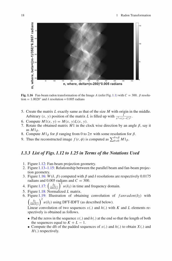
Fig. 1.16 Fan-beam radon transformation of the Image A (refer Fig. 1.1) with C = 300, β resolu-tion = 1.0028◦ and δ resolution = 0.005 radians
5. Create the matrix L exactly same as that of the size M with origin in the middle.Arbitrary (x, y) position of the matrix L is filled up with 1
x2+(y−C)2 .6. Compute M1(x, y) = M(x, y)L(x, y).7. Rotate the obtained matrix M1 in the clock wise direction by an angle β, say it
as M1β .8. Compute M1β for β ranging from 0 to 2π with some resolution for β.9. Thus the reconstructed image f (r, φ) is computed as
∑θ=βθ=0 M1β .
1.3.3 List of Figs. 1.12 to 1.25 in Terms of the Notations Used
1. Figure 1.12: Fan-beam projection geometry.2. Figure 1.13–1.15: Relationship between the parallel beam and fan-beam projec-
tion geometry.3. Figure 1.16: W (δ, β) computed with β and δ resolutions are respectively 0.0175
radians and 0.005 radians and C = 300.
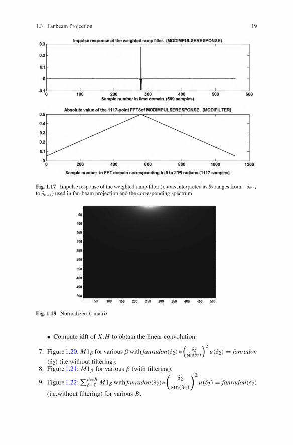
4. Figure 1.17:(
δ2sin(δ2)
)2u(δ2) in time and frequency domain.
5. Figure 1.18: Normalized L matrix.6. Figure 1.19: Illustration of obtaining convolution of f anradon(δ2) with(
δ2sin(δ2)
)2u(δ2) using DFT-IDFT (as described below).
Linear convolution of two sequences x(.) and h(.) with K and L elements re-spectively is obtained as follows.
• Pad the zeros in the sequence x(.) and h(.) at the end so that the length of boththe sequences equal to K + L − 1.
• Compute the dft of the padded sequences of x(.) and h(.) to obtain X (.) andH(.) respectively.
1.3 Fanbeam Projection 19
Fig. 1.17 Impulse response of the weighted ramp filter (x-axis interpreted as δ2 ranges from −δmaxto δmax) used in fan-beam projection and the corresponding spectrum
Fig. 1.18 Normalized L matrix
• Compute idft of X.H to obtain the linear convolution.
7. Figure 1.20: M1β for various β with fanradon(δ2)∗(
δ2sin(δ2)
)2u(δ2) = fanradon
(δ2) (i.e.without filtering).8. Figure 1.21: M1β for various β (with filtering).
9. Figure 1.22:∑β=B
β=0 M1β with fanradon(δ2)∗(
δ2
sin(δ2)
)2
u(δ2) = fanradon(δ2)
(i.e.without filtering) for various B.

20 1 Radon Transformation
Fig. 1.19 Illustration of obtaining the filtered fan-beam projection data from the original fan-beamprojection data for the angle β = 0.07 radian
Fig. 1.20 Illustration of original fan-beam backprojected images obtained from the OFBPD forβ = 0.0175, 0.7156, 1.4137, 2.1118, 2.8100, 3.5081, 4.2062, 4.9044, 5.6025 radians. (Note thatfan-beam reconstructed images are computed for all β ranging from 0 to 6.2657 with the resolutionof 0.0175 radians)

1.3 Fanbeam Projection 21
Fig. 1.21 Illustration of filtered fan-beam backprojected images obtained from the FFBPD forβ = 0.0175, 0.7156, 1.4137, 2.1118, 2.8100, 3.5081, 4.2062, 4.9044, 5.6025 radians. (Note thatfan-beam reconstructed images are computed for all β ranging from 0 to 6.2657 with the resolutionof 0.0175 radians)
Fig. 1.22 Illustration of reconstruction of the image obtained by cumulative summation of originalfan-beam backprojected images

22 1 Radon Transformation
Fig. 1.23 Illustration of reconstruction of the image obtained by cumulative summation of filteredfan-beam backprojected images
Fig. 1.24 Final reconstructed image obtained from original fanbeam projection with C = 300

1.3 Fanbeam Projection 23
Fig. 1.25 Final reconstructedimage obtained from filteredfanbeam projection withC = 300
10. Figure 1.23:∑β=B
β=0 M1β for various B (with filtering).11. Figure 1.24: Final fan-beam reconstructed image f (r, φ) without filtering.12. Figure 1.25: Final fan-beam reconstructed image f (r, φ) with filtering.
1.3.3.1 Fanbeamprojection.m
%load the original imageload VASIGIMAGEC=C(1:1:255,1:1:255);C=[zeros(128,511);zeros(255,128) C zeros(255,128);
zeros(128,511)];C=double(C)/255;figureD=300;maxiangle=atan(256/((D-255)+1));B=zeros(511,511);j=1;range1=0:0.005:round(maxiangle/0.005)*0.005;range2=sort(-1*range1);ang=0:(2*pi)/359:2*pi;angdeg=(ang/pi)*180;for ang=angdeg(1:1:length(angdeg)-1)t=0;i=1;A1=imrotate(C,ang,’crop’);%Computation of Betabeta(j)=ang;%Computation of deltadelta=[range2 range1(2:1:length(range1))];for range=[range2 range1(2:1:length(range1))];

24 1 Radon Transformation
s=0;%X and Y positionsX=-255:1:255;Y=round((D-X)*tan(range));Y1=-1*(Y+256)+512;X1=-1*(X+256)+512;COL{i}=[X1;Y1];for u=1:1:511if(X1(u)<=511&Y1(u)<=511&Y1(u)>0)B(X1(u),Y1(u))=255;s=s+A1(X1(u),Y1(u));endendt(i)=s;i=i+1;endfanbeam{j}=t;t=0;j=j+1;endfigurecolormap(gray)imagesc(B)fanbeamprojection=fanbeam;%Fan beam reconstruction%4.Multiply with the modified ramp filter%5.Weighted back projectionDATA=zeros(511,511);RECONSTRUCTEDMATRIX=zeros(511,511);%Computation of weight matrix Lˆ(-2)for i=1:1:511
for j=1:1:511k=-i+512-256;l=-j+512-256;
L_MATRIX(j,i)=sqrt(kˆ2+(D-l)ˆ2);end
endL_MATRIX=L_MATRIX.ˆ(-2)/max(max(L_MATRIX.ˆ(-2)));DATA=0;figurecolormap(gray)%Design of the weighted ramp filterdeltaterm=((delta.ˆ2)./(sin(delta).ˆ2));deltaterm(280)=1;MODIMPULSERESPONSE=(1/2)*fir2(558,[0:1/558:1],[0.1:0.9/558:1],
hann(559)).*deltaterm;%Fourier tansformation of the weighted ramp filter
after zero padding.MODFILTER=fft(MODIMPULSERESPONSE,1117);for k=1:1:359RECONSTRUCTEDMATRIX=zeros(511,511);%Compuation of the Modified fanbeam projectionfanbeamprojection_modified1{k}=(D*cos(delta)).

1.3 Fanbeam Projection 25
*fanbeamprojection{k};%Fourier transformation of the modified fan beam projectionafter zero padding
fanbeamprojection_modified2{k}=fft(fanbeamprojection_modified1{k},1117);
%Multiplication with the fourier tansformationof the weighted ramp
%filter after zero padding%Computation of inverese fourier transformationfanbeamprojection_modified3{k}=ifft(fanbeamprojection_
modified2{k}.*MODFILTER);%Backprojection in the fanbeam structurel=1;for range=(-2*maxiangle):(4*maxiangle)/1116:(2*maxiangle)X=-255:1:255;Y=round((D-X)*tan(range));Y1=-1*(Y+256)+512;X1=-1*(X+256)+512;for u=1:1:511if((X1(u)<=511)&(Y1(u)<=511)&(Y1(u)>0))RECONSTRUCTEDMATRIX(X1(u),Y1(u))=fanbeamprojection_
modified3{k}(l);endendl=l+1;end%Multiplication with the weight matrixRECONSTRUCTEDMATRIX=RECONSTRUCTEDMATRIX.*L_MATRIX;%Obtaining the reconstructed matrix for beta(k)RECONSTRUCTEDMATRIX=imrotate(RECONSTRUCTEDMATRIX,
-beta(k),’crop’);imagesc(RECONSTRUCTEDMATRIX)pause(0.5)DATA=DATA+RECONSTRUCTEDMATRIX;endfigurecolormap(gray(256))imagesc(DATA)

Chapter 2Magnetic Resonance Imaging
2.1 Bloch Equation
The concept of MRI physics is described by the bloch equations. Consider the weak
magnetic field→
M(t) kept at an angle α (in the anticlockwise direction) with the
strong magnetic field→
B(t) (which is kept in the z-direction as shown in the Fig. 2.1).The interaction between these magnetic fields end up with the torque (The rate of
change of angular momentum→
J(t) is the torque) on the weaker magnetic field→
B(t)as mentioned in the Eq. (2.1).
→J(t)
dt= →
M(t) × →B(t) (2.1)
Note that the magnetic moment is proportional to the angular momentum (i.e)→
M(t) =γ
→J(t)⇒ d
→M(t)dt = γ
→M(t) × →
B(t), where γ is gyromagnetic ratio of the magnetic
moment→
M(t).
Let→
M(t)= Mx(t)̂i + My(t)̂j + Mz(t)̂k and→
B(t)= Bx(t)̂i + By(t)̂j + Bz(t)̂k withBx(0) = 0, By(0) = 0 and Bz(0) = B0
⇒ →M(t) × →
B(t)=⎡⎣ i j k
Mx(t) My(t) Mz(t)0 0 B0
⎤⎦
This further implies,
dMx(t)
dt= γ My(t)B0 (2.2)
E. S. Gopi, Digital Signal Processing for Medical Imaging Using Matlab, 27DOI: 10.1007/978-1-4614-3140-4_2, © Springer Science+Business Media New York 2013
28 2 Magnetic Resonance Imaging
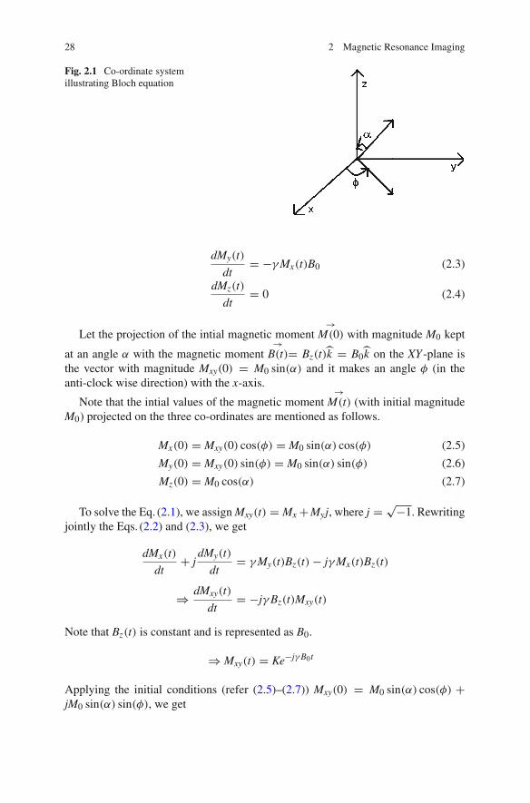
Fig. 2.1 Co-ordinate systemillustrating Bloch equation
dMy(t)
dt= −γ Mx(t)B0 (2.3)
dMz(t)
dt= 0 (2.4)
Let the projection of the intial magnetic moment→
M(0) with magnitude M0 kept
at an angle α with the magnetic moment→
B(t)= Bz(t)̂k = B0̂k on the XY -plane isthe vector with magnitude Mxy(0) = M0 sin(α) and it makes an angle φ (in theanti-clock wise direction) with the x-axis.
Note that the intial values of the magnetic moment→
M(t) (with initial magnitudeM0) projected on the three co-ordinates are mentioned as follows.
Mx(0) = Mxy(0) cos(φ) = M0 sin(α) cos(φ) (2.5)
My(0) = Mxy(0) sin(φ) = M0 sin(α) sin(φ) (2.6)
Mz(0) = M0 cos(α) (2.7)
To solve the Eq. (2.1), we assign Mxy(t) = Mx +Myj, where j = √−1. Rewritingjointly the Eqs. (2.2) and (2.3), we get
dMx(t)
dt+ j
dMy(t)
dt= γ My(t)Bz(t) − jγ Mx(t)Bz(t)
⇒ dMxy(t)
dt= −jγ Bz(t)Mxy(t)
Note that Bz(t) is constant and is represented as B0.
⇒ Mxy(t) = Ke−jγ B0t
Applying the initial conditions (refer (2.5)–(2.7)) Mxy(0) = M0 sin(α) cos(φ) +jM0 sin(α) sin(φ), we get
2.1 Bloch Equation 29
⇒ Mxy(t) = (M0 sin(α) cos(φ) + jM0 sin(α) sin(φ))e−jγ B0t
⇒ Mxy(t) = M0 sin(α)ejφe−jγ B0t
⇒ Mx(t) = M0 sin(α) cos(φ − γ B0t) = M0 sin(α) cos(−γ B0t + φ) (2.8)
My(t) = M0 sin(α) sin(φ − γ B0t) = M0 sin(α) sin(−γ B0t + φ) (2.9)
Mz(t) = M0 cos(α) (2.10)
2.2 Comment on the Equations 2.8–2.10
When the weak initial magnetic moment→
M(0) with magnitude M0 is kept at an
angle α with the strong constant magnetic moment→
B(t)= Bz(t)̂k = B0̂k, due tobloch equation, magnetic moment in the z-direction remains unchanged. But themagnetic moment in the x-direction and the y-direction oscillates with the angularfrequency of γ B0 radians or γ B0
2πHz with maximum amplitude M0 sin(α). Thus at
any particular time instant, the magnitude of the resultant magnetic moment on theX–Yplane is constant and is equal to M0 sin(α). Also note that at any particular timeinstant t, the resultant magnetic moment on the XY -plane is making an angle withmagnitude (−γ B0t + φ) with the x-axis measured in the anti-clock wise direction.As time goes, the magnitude of the angle is increasing. This implies the resultantvector on the XY -plane rotates in the anti-clock wise direction (when viewed in the zdirection) with the frequency γ B0. This frequecy is called larmor frequeny in radiansand it is computed as γ B0
2πin Hz. For the constant strong magnetic moment B0, the
larmor frequency purey depends on the gyromagnetic ratio of the magnetic moment→
B(t). Note that the magnitude of the resultant magnetic moment in the XY -plane(transverse plane) is directly proportional to the angle α. Note:Clock wise directionis identified with respect to the view point in the direction of − z axis (refer Fig. 2.1).
2.3 The Larmor Frequency and the Tip Angle α
In general, resultant magnetic moment (without externel strong magnetic moment)obtained in the macroscopic level in the human body is zero. When the human bodyis kept under the constant strong magnetic moment of B0 in the z-direction. Theresultant magnetic moment in the macroscopic level is aligned to the direction ofthe external strong magnetic moment (i.e) z-direction. When it is disturbed to bringthe resultant magnetic moment to make an angle α (measured anti-clock-wise direc-tion) with the z-axis, there exists the resultant anti-clock-wise rotating magneticmoment in the transverse plane (due to bloch equations), that rotates with the fre-quency 42.58 Mhz, when B0 is 1 Tesla.

30 2 Magnetic Resonance Imaging
2.3.1 Disturbance to obtain Non-Zero α Value
The external field (apart from the strong constant magnetic moment B0) is applied for
the short duration (τ ) in such a way that the resultant magnetic moment→
E(t) is rotating
exactly with the larmor frequency of the magnetic moment→
M(t) to be disturbed. It
is noted that the macro magnetic moment→
M(t) obtained using the hydrogen atomsthat are aligned in the z-direction due to the availibility of strong magnetic moment
B0 in the z-direction. The interaction between the magnetic moment→
M(t) aligned
in the z-direction with magnitude M0 and the rotating magnetic moment→
E(t) onthe transverse plane is described by the bloch equations as described below. The
strength of the magnetic moment→
E(t) is strong compared with the natural magnetic
moment→
M(t) available in the human body that are aligned initially in the z-direction.
Rewriting the bloch equation using→
M(t) and→
E(t), we get the following.
→dJ(t)
dt= →
M(t) × →E(t) (2.11)
⇒ →M(t) × →
E(t) =⎡⎣ i j k
0 0 Mz(t)Ex(t) Ey(t) 0
⎤⎦ ⇒
dMx(t)
dt= γ Ey(t)M0 = γ E0 cos(−γ B0t + θ)M0 (2.12)
dMy(t)
dt= γ Ex(t)M0 = γ E0 sin(−γ B0t + θ)M0 (2.13)
dMz(t)
dt= 0 (2.14)
Solving the Eqs. (2.12)–(2.14) as described in the Sect. 2.1, we still get the resultant
magnetic moment→
M(t) lies only in the z-direction. It is noted from the equationsthat the transverse magnetic moment is zero due to the initial conditions Mx(0) =0, My(0) = 0.
But in practice, due to the external field, there is the disturbance in the resultantmagnetic moment and there exist very low magnitude Mx and My component thatrotates in the larmor frequency due to the existance of strong field B0 as described in
the Sect. 2.1. Now consider the interaction between the magnetic fields→
E(t) (which
has Ex(t) and Ey(t) components) and→
B(t) (which has Bz(t) = B0 component) on the
magnetic moment→
M(t) which have all the three components.
→dM(t)
dt= γ
→M(t) ×(
→E(t) + →
B(t)) (2.15)

2.3 The Larmor Frequency and the Tip Angle α 31
The resultant magnetic moment→
M(t) depends upon the first term and the second
term of the RHS of the (2.16) independently. The resultant→
M(t) due to the secondterm ends up with Mx(t), My(t) and Mz(t) components as described in the Eqs. (2.9)–(2.11). Note that the z-component of the resultant vector is constant due to the second
term. Now the magnetic moment→
M(t) due to the first term is obtained as follows.Rewriting (2.15) with only first term of the RHS as
→dM(t)
dt= γ
→M(t) ×(
→E(t)) (2.16)
⇒ →M(t) × →
E(t) =⎡⎣ i j k
Mx(t) My(t) Mz(t)Ex(t) Ey(t) 0
⎤⎦ ⇒
dMx(t)
dt= −γ Ey(t)Mz(t) = −γ E0 sin(−γ B0t + θ)M0 cos(α) (2.17)
dMy(t)
dt= γ Ex(t)Mz(t) = γ E0 cos(−γ B0t + θ)M0 cos(α) (2.18)
dMz(t)
dt= γ (Mx(t)Ey(t) − My(t)Ex(t)) (2.19)
Solving the Eqs. (2.17)–(2.19) as described in Sect. 2.1, we get the following.
dMx(t)
dt+ j
dMy(t)
dt= γ E0M0 cos(α)(− sin(−γ B0t + θ)
+ jcos(−γ B0t + θ)) (2.20)
⇒ dMxy(t)
dt= jγ E0M0 cos(α)ej(−γ B0t+θ) (2.21)
⇒ Mxy(t) = −E0M0 cos(α)
B0ej(−γ B0t+θ)K,
where K is the constant.As Mxy(0) = M0 sin(α) cos(φ) + jM0 sin(α) sin(φ) = M0 sin(α)e(jφ) we get K
as follows.
Mxy(0) = −E0M0 cos(α)
B0e(jθ)K
⇒ −E0M0 cos(α)
B0cos(θ)K = M0 sin(α) cos(φ)
Also,
32 2 Magnetic Resonance Imaging
−E0M0 cos(α)
B0sin(θ)K = M0 sin(α) sin(φ)
⇒ K = −B0
E0tan(α)ej(φ−θ)
⇒ Mxy(t) = −E0M0 cos(α)
B0ej(−γ B0t+θ) −B0
E0tan(α)ej(φ−θ)
⇒ Mxy(t) = M0 sin(α)ej(−γ B0t+φ)
Note that, the transverse component is not changed due to the external field→
E(t).What we achieved is that the transverse magnetic moment Mxy(t) due to the external
field→
E(t) is in phase as that of the transvere component obtained using the static
magnetic field B0. The resultant transverse magnetic moment due to B0 and→
E(t) isgiven as
Mxy(t) = 2M0 sin(α)ej(−γ B0t+φ) (2.22)
The effect of the external magnetic moment→
E(t) on the z-component of the magnetic
moment→
M(t) is obtained by solving (2.19) as shown below.
dMz(t)
dt= γ (Mx(t)Ey(t) − My(t)Ex(t))
= γ M0E0 sin(α)(sin(−γ B0t + θ) cos(−γ B0t + φ)
− cos(−γ B0t + θ) sin(−γ B0t + φ))
= γ M0 sin(α)E0 sin(−γ B0t + θ − (−γ B0t + φ)
Thus
dMz(t)
dt= γ M0 sin(α)E0 sin(θ − φ) (2.23)
⇒ Mz(t) = γ M0 sin(α)E0 sin(θ − φ)t + Mz(0) (2.24)
Applying the initial condition Mz(0) = M0 cos(α) in (2.24), we get Mz(t) =γ M0 sin(α)E0 sin(θ − φ)t + M0 cos(θ). Recall that the z-component due to B0 isM0 cos(α) and hence resultant z-component is obtained as follows
Mz(t) = γ M0 sin(α)E0 sin(θ − φ)t + 2M0 cos(α) (2.25)
It is also noted that the resultant z-component with external field B1 (instead ofB0) is given as
Mz(t) = γ M0 sin(α)E0 sin(−γ (B1 − B0) + θ − φ)t + 2M0 cos(α) (2.26)
2.3 The Larmor Frequency and the Tip Angle α 33
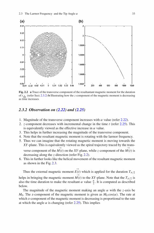
Fig. 2.2 a Trace of the transverse component of the resultantant magnetic moment for the durationof t π
200(refer Sect. 2.3.2) b Illustrating how the z-component of the magnetic moment is decreasing
as time increases
2.3.2 Observation on (2.22) and (2.25)
1. Magnitude of the transverse component increases with α value (refer 2.22).2. z-component decreases with incremental change in the time t (refer 2.25). This
is equivalently viewed as the effective increase in α value.3. This helps in further increasing the magnitude of the transverse component.4. Note that the resultant magnetic moment is rotating with the larmor frequency.5. Thus we can imagine that the rotating magnetic moment is moving towards the
XY -plane. This is equivalently viewed as the spiral trajectory traced by the trans-
verse component of the→
M(t) on the XY -plane, while z-component of the→
M(t) isdecreasing along the z-direction (refer Fig. 2.2).
6. This in further looks like the helical movement of the resultant magnetic momentas shown in the Fig. 2.3.
Thus the external magnetic moment→
E(t) which is applied for the duration Tπ/2
helps in bringing the magnetic moment→
M(t) to the XY -plane. Note that the Tπ/2 isalso the time duration to make the resultant α value π
2 . It is computed as describedbelow.
The magnitude of the magnetic moment making an angle α with the z-axis beM0. The z-component of the magnetic moment is given as M0 cos(α). The rate atwhich z-component of the magnetic moment is decreasing is proportional to the rateat which the angle α is changing (refer 2.25). This implies

34 2 Magnetic Resonance Imaging
Fig. 2.3 Trace of the resultant magnetic moment in 3D for the duration of t π200
(refer Sect. 2.3.2)
− M0 sin(α)dα
dt= γ M0 sin(α)E0 sin(θ − φ) (2.27)
⇒ dα
dt= −γ E0 sin(θ − φ) (2.28)
⇒ α(t) = −t∫
0
γ E0 sin(θ − φ)dt (2.29)
If the external field is B1, then α(t) is computed as follows (refer 2.26).
α(t) = −t∫
0
γ E0 sin(−γ (B1 − B0) + θ − φ)dt (2.30)
2.3.2.1 resmagneticmoment.m
gamma=2*pi*42.58*10ˆ6;E0=0.0001;M0=1;B0=1;phi=0.1;theta=0.2;x=[];y=[];z=[];duration=5.8713*10ˆ(-5);for t=0:(duration/100000):(duration/100)alpha1= E0*gamma*t;x=[x 2*M0*sin(alpha1)*cos(-gamma*B0*t+phi)];

2.3 The Larmor Frequency and the Tip Angle α 35
y=[y 2*M0*sin(alpha1)*sin(-gamma*B0*t+phi)];z=[z gamma*M0*sin(alpha1)*E0*sin(theta-phi)*t+2*M0*cos(alpha1)];endfigureplot3(x,y,z)figuresubplot(1,2,1)plot(x,y)subplot(1,2,2)plot(z)
2.4 Trick on MRI
The external magnetic moment→
E(t) is applied for the duration Tπ/2 to bring theresultant magnetic moment to the transverse plane as described in the Sect. 2.3. After
that, when→
E(t) is removed, the resultant magnetic moment has to rotate with constantmagnitude in the XY -plane with the larmor frequency. But in nature, transversecomponent decreases and reaches zero after some time. This is called spin relaxation.This is due to the spin–spin interactions between the micro-level magnetic momentsavailable in the human body. The time required to obtain (1/e) times the initial valueof the transverse component after the removal of the external magnetic moment(represented as T2) depends on the characteristics of the tissues of human body.The resultant transverse magnetic moment during relaxation (free induction decay(FID)) is recorded using the receiver antenna. This is used to obtain T2 MRI andproton-density MRI images.
In the same fashion, longituidanal component gradually increases and attains themaximum value. This is due to spin-lattice interactions in the micro level magneticmoments of the human body. The rate at which lognituidanal component reaches themaximum value is described by the time constant T1 (depends on the characteristicsof the tissues of the human body). Usually T1 � T2. After sufficient time (to nullifythe influence of existing transverse component), longitudanal component is flippedto the transverse component and the corresponding FID is measured. This is used toobtain the T1 MRI image. Note that in all the cases (T1, T2 and proton-density) MRIimages, the receiver records only the transverse components of the magnetic fieldduring relaxation. The complete description is given in Sect. 2.8.
2.5 Selecting the Human Slice and the CorrespondingExternal RF Pulse
When the external RF frequency is same as that of the larmour frequency, we areable to get the transverse component of the magnetic field. When the completehuman body is kept under the identical strong magnetic moment B0, the recorded
36 2 Magnetic Resonance Imaging
FID signal corresponds to the complete human body. But we need to get the imageof the particular slice. This is obtained using the concept of Gradient. Let us assumethat we need to image the particular slice of the human body along the z-axis. Weapply the gradient magnetic moment such that the z-component of the static magneticfield Bz(z) is the function of z. The resultant z-component of the magnetic momentis given as Bz(z) = Gzz + K , where Gz is the z-gradient and K is the constant. Theconstant is chosen such that at the required point z, the magnitude of the magneticmoment is B0. (i.e)
Bz(z) = Gz(z − z̄) + B0 (2.31)
Recollect that the external field used to disturb the orignal magnetic moment M(t)(to obtain non-zero alpha) which are kept under the strong magnetic field B0 in thez-axis is given as Ex(t) = −γ E0 sin(−γ B0t+θ) and Ey(t) = −γ E0 cos(−γ B0t+θ)
(refer 2.12 and 2.13). We can still use the same external field for disturbance. Butit controls the slice corresponding to the frequency γ B0. In practice it is difficultto generate such signals. so the alternate technique is to choose the slice with pre-determined thickness. Let us assume, we need to image the slice corresponds to themagnetic field ranging between Bz1 and Bz2 , where z̄ = (z1+z2)
2 . In this case, theexternal magnetic field is chosen such tha Tα for all the magnetic moments of thechosen slice is identical. It is given as follows.
Ex(t) = −AΔvγ sinc(Δvt) sin(−γ B0t + θ) (2.32)
Ey(t) = −AΔvγ sinc(Δvt) cos(−γ B0t + θ) (2.33)
It is noted that the external field is having only transverse comonents. Also note
that the Δv is the bandwidth in Hz, which is computed asγ (Bz1−Bz2 )
2π. Using (2.31)
we obtain, Δv = γ Gz(z1−z2)2π
. It is noted Δv � B0γ2π
. Using this condition, blochequations with external fields (refer Sect. 2.3.2 and appendix 1) is solved to obtainthe following equation for α(t).
α(t, z) = −t∫
0
AΔvγ sinc(Δvt) sin(−γ (Bz(z) − B0) + θ − φ)dt (2.34)
Note that the time instant at which t = 0 is the starting time at which the externalfield is applied. In (2.28), the amplitude (envelope) of the external field is constant. Butin this case, the starting time is properly chosen as the envelope is the AΔvsinc(Δvt)function. The sinc function is given as sinc(Δvt) = sin πΔvt
πΔvt and is maximum att = 0.
Suppose let us assume the case we are applying the AΔvsinc(Δvt) pulse for theduration from −∞ to ∞ (which is not practical). The obtained α values as thefunction of z (refer Sect. 2.3.2) is obtained as follows.
2.5 Selecting the Human Slice and the Corresponding External RF Pulse 37
α(z) = −∞∫
−∞AΔvγ sinc(Δvt) sin(−γ Gz(z − z̄)t + θ − φ)dt (2.35)
⇒ α(z) = Im
⎛⎝−
∞∫
−∞AΔvγ sinc(Δvt)ej(−γ Gz(z−z̄)t+θ−φ)dt
⎞⎠ (2.36)
Consider the following equation as the fourier transformation of the AΔvγ sin c(Δvt)ej(θ−φ) with frequency γ Gz(z − z̄) (in radians)
−∞∫
−∞AΔvγ sinc(Δvt)ej(−γ Gz(z−z̄)t+θ−φ)dt (2.37)
Solving we get the following.
α(z) = −Aγ sin(θ − φ)rect
(γ Gz(z − z̄)
2πΔv
)(2.38)
⇒ α(z) = −Aγ sin(θ − φ)rect
((z − z̄)
Δz
)(2.39)
where Δz = 2πΔvγ Gz
Thus the obtained α for the entire slice is constant. But in practice the sinc envelopeis not applied for the infinite duration. It is applied during the duration −τp/2 toτp/2. This makes the α(z) profile not perfectly flat. From signal processing, weunderstand that FT(rect( t
τp)AΔvγ sinc(Δvt)) computed with frequency γ Gz(z−z̄) is
same as that of the convolution of FT(rect( tτp
) (computed with frequency γ Gz(z− z̄))and FT(AΔvγ sinc(Δvt)) (computed with frequency γ Gz(z − z̄)). This implies thefollowing expression for α(z).
α(z) = −Aγ sin(θ − φ)rect((z − z̄)
Δz) ∗ τpsinc(τpγ Gz(z − z̄)) (2.40)
Thus using the external field (2.32) and (2.33), we obtain almost the identical α overthe region of interest (slice region). Thus the particular slice of the human body alongthe z-axis is selected. Note that external field is applied over the duration −τp/2 toτp/2.
At the end of time instant τp/2 (after acquiring required α value), Mxy(t, z) isobtained as follows (refer (2.22)).
Mxy(τp/2) = 2M0 sin(ατp/2)ej(−γ Bz(z)τp/2+φ) (2.41)
⇒ Mxy(τp/2) = 2M0 sin(ατp/2)ej(−γ (Gz(z−z̄)+B0)τp/2+φ) (2.42)
38 2 Magnetic Resonance Imaging
Note that the phase component of (2.42) varies with z as ej(−γ (Gz(z−z̄)τp/2)). To nullifythis, negative z-gradient −Gz (along with the existent strong magnetic field B0) isapplied. This is known as Refocussing gradient. Note that the external field (2.32)and (2.33) are removed. When the resultant magnetic moment is having non-zero α
and are kept with the strong magnetic field −(Gz(z − z̄) + B0) for the time durationτp/2, rotating transverse component (after τp/2) is obtained and is given as follows.
2M0 sin(ατp/2)ej(−γ (Gz(z−z̄)+B0)τp/2+φ)ej(−γ (−Gz(z−z̄)+B0)τp/2) (2.43)
⇒ 2M0 sin(ατp/2)ej(−γ (B0)τp+φ) (2.44)
Thus the resultant phase component is constant throughout the slice (not the functionof z). But note that there is still strong magnetic field B0 available in the z-axis. Hencetransverse magnetic moments along the slice are having the same phase, havingnon-zero α value and are under the constant magnetic field B0. Hence transversecomponents of the magnetic field along the slice follows the equation as mentionedbelow.
2M0 sin(ατp/2)ej(−γ (B0)τp+φ)ej(−γ (B0)t) (2.45)
In (2.45), t = 0 corresponds to τp in the time scale t′, where t′ = 0 correspondsto the middle of the sinc pulse applied. As described in the Sect. 2.4, the resultanttransverse component (refer 2.46) gradually decreases due to spin–spin interations.This interactions start at the moment when there is non-zero α value. so at timet = 0 (middle of the RF pulse) itself, the transverse components decreses with timeconstant T2. If there is no refocussing gradient and other externally disturbing fields,the disturbance in the transverse component is only due to spin–spin interaction,which is completely described by the time constant T2. For instance, after applyingrefocussing gradient, the transverse component of the magnetic moment (includingthe effect of spin–spin relaxation) is given as follows.
2M0 sin(ατp/2)ej(−γ (B0)τp+φ)ej(−γ (B0)t)e
−tT2(x,y) e
−τpT2(x,y) (2.46)
Note that T2 is the function of (x, y) due to different physical characteristics of thetissues. The transverse component of the signal is sampled at some time instant TR
(read-out time instant) depends on the factor T2(x, y) and helps for T2-MRI imagingtechnique.
2.5.1 Summary of the Section 2.5
1. Apply positive z-gradient Gz to select the slice of the human body along the z-axis.2. RF pulse AΔvγ sinc(Δvt)rect( t
τp) is applied (Note that the duration is between
−τp/2 and τp/2) to obtain the identical α throughout the slice.

2.5 Selecting the Human Slice and the Corresponding External RF Pulse 39
3. Negative z-gradient −Gz (refocussing gradient) (for the duration τp/2 to τp) isapplied to achieve the identical strong magnetic field throughout the slice, bynullifying the phase introduced during RF exitation.
4. Step 3 helps in obtaining the transverse magnetic components within the selectedslice (in all (x, y) co-ordinates) to rotate with the larmour frequency with zerophase difference for a moment.
5. But the transverse component gradually decreases with time due to spin–spininteraction. This is known as relaxation. The rate at which the transverse compo-nents decreases depend on the location (with differnet tissue property at (x, y))described by the time constant T2.
6. Transverse components are assumed to start decaying from the time instant t = 0,which is the middle of the applied RF pulse.
7. We need to measure the transverse component during relaxation which acts asthe first step to obtain MRI image as described in the Sect. 2.6
2.6 Measurement of the Transverse Component Usingthe Receiver Antenna
In general, the transverse magnetic moment and the longituidanal magnetic momentduring the readout phase are given as follows.
Mxy(x, y, t) = Mxy(x, y, 0+)ej(−γ (B0)t+φ)e−t
T2(x,y)
Mxy(x, y, 0+) = Mz(x, y, 0−) sin(α(x, y))
Mz(x, y, t) = Mz(x, y, 0+)e−t/T1 + (1 − e−t/T1)B0
Mz(x, y, 0+) = Mz(x, y, 0−) cos(α(x, y))
To obtain the image that describes the Tx,y property of the sliced XY plane(selected slice plane), readout time should be chosen such that the α(x, y) value mustbe constant throughout the plane. Rewriting the equations with constant α(x, y) is asfollows.
Mxy(x, y, t) = Mxy(x, y, 0+)ej(−γ (B0)t+φ)e−t
T2(x,y) (2.47)
Mxy(x, y, 0+) = Mz(x, y, 0−) sin(α) (2.48)
Mz(x, y, t) = Mz(x, y, 0+)e−t/T1 + (1 − e−t/T1)B0 (2.49)
Mz(x, y, 0+) = Mz(x, y, 0−) cos(α) (2.50)

40 2 Magnetic Resonance Imaging
2.6.1 Observation on (2.47)–(2.50)
1. The time instant t = 0 in (2.47) is the starting time at which the receiver startsreceiving the signal. This is otherwise called as the starting time instance of thereadout phase.
2. Note that the transverse component is rotating with identical larmour frequencyat all (x,y) positions. This is achieved with the identical strong magnetic field (inthe z-axis) throughout the slice.
3. The amplitude Mxy(x, y, 0+) is the function of (x, y) as it involves the hidden
term e−t
T2(x,y) from the time instance of the middle of the RF pulse.4. Hence if the receiver is designed to receive the transverse component as the
function of (x, y), the image completely describes the T2(x, y) characteristics ofthe sliced tissue.
2.6.2 Receiver to Receive the Transverse Component
The transverse component M(x, y, t) is represented as the vector [Mx,t My,t]. UsuallyMx,t component is sensed as the voltage induced in the the receiver coil as describedbelow. When the receiver coil is excited with the external source to generate thetransverse magnetic moment represented as the vector [1 0] and are kept in thetransverse magnetic moment (to be sensed) represented as the vector [Mx,t My,t], thevoltage is induced in the coil as follows.
v(t) = − d
dt
∫
x
∫
y
[Mx,t My,t] · [1 0]dxdy (2.51)
The generalized expression for the transverse component of the magnetic momentis given as
M(x, y, t) = (Mr + jMi)e−j(γ B0t−φ) (2.52)
⇒ v(t) = − d
dt
∫
x
∫
y
[(Mr cos(γ B0t − φ) + Mi sin(γ B0t − φ))
(−Mr sin(γ B0t − φ) + Mi cos(γ B0t − φ))] · [1 0]dxdy (2.53)
⇒ v(t) = γ B0
∫
x
∫
y
(Mr sin(γ B0t − φ) − Mi cos(γ B0t − φ))dxdy (2.54)
It is possible to obtain Mr and Mi as follows.

2.6 Measurement of the Transverse Component Using the Receiver Antenna 41
1. Multiply v(t) with sin(γ B0t − φ) and pass it through the low pass filter to obtainKγ B0
∫x
∫y Mrdxdy component, where K is the constant. Note that phase lock is
also required.2. Similarly, multiply v(t) with − cos(γ B0t − φ) and pass it through the low pass
filter to obtain Kγ B0∫
x
∫y Midxdy component.
3. Thus the complex numbr C∫
x
∫y(Mr + jMi)dxdy can be stored in the computer
as the complex number, where C is real constant.4. In MRI imaging, Mr, vMi are usually the function of time which are represented
as Mr(t), Mi(t). The frequency content of the signals Mr(t) and Mi(t) are com-paritively very less when compared with the frequency γ B0. Hence the sameprocedure (as described in 1 and 2) can be used to obtain the complex numberC1
∫x
∫y(Mr(t) + jMi(t))dxdy as the function of time, where C1 is some arbitrary
real constant.5. Sampling the signal at any time instant gives the constant complex number, which
can be stored in the computer.
2.7 Sampling the MRI Image in the Frequency Domain
We understand that the the receiver is capable of receiving the real and imaginarycomponent of the signal s(t) (funtion of t) mentioned in (2.55). Recall that theMxy(x, y, 0+) is the complex quantity.
s(t) =∞∫
−∞
∞∫
−∞Mxy(x, y, 0+)ej(φ)e
−tT2(x,y) dxdy (2.55)
Suppose that the external strong magnetic field (in the z-axis) is made as the functionof x and y (i.e) Bz(x, y) = B0 + xgx + ygy (Note that gx and gy are constants),we get
s(t) =∞∫
−∞
∞∫
−∞Mxy(x, y, 0+)ej(−γ (Bz(x,y))t+φ)e
−tT2(x,y) dxdy (2.56)
⇒ s(t) =∞∫
−∞
∞∫
−∞Mxy(x, y, 0+)ej(−γ (B0+xgx+ygy)t+φ)e
−tT2(x,y) dxdy (2.57)
By varying the constants gx gy described by the variables Gx, Gy respectively, thesame receiver is now capable of obtaining the real and imaginary component of thesignal s(Gx, Gy, t).
42 2 Magnetic Resonance Imaging
s(Gx, Gy, t) =∞∫
−∞
∞∫
−∞Mxy(x, y, 0+)ej(−γ (xGx+yGy)t+φ)e
−tT2(x,y) dxdy (2.58)
Sample the obtained complex signal at the middle of the readout time duration(Treadout/2), which is the function of Gx and Gy). By vaying different values of Gx
and Gy we obtain the real matrix R(Gx, Gy) and the imaginary matrix I(Gx, Gy).Note that Gx and Gy ranges from the −Gmax/2 to Gmax/2 with the step incrementof Gmax/L, where L is the level number. Let us assume that the complete slice hasto pictured with 101 × 101 pixel resolution, then the Gx and Gy must have L = 101.This is equivalent to sampling the image in frequency domain.
C(Gx, Gy) = R(Gx, Gy) + jI(Gx, Gy) (2.59)
=∞∫
−∞
∞∫
−∞Mxy(x, y, 0+)ej(−γ (xGx+yGy)(Treadout/2)+φ)e
−(Treadout/2)
T2(x,y) dxdy
(2.60)
Apply the linear map of the variable Gx to U and Gx to V as Gx = (Gmax/(L −1))U(Gmax/2) and Gy = (Gmax/(L − 1))V − (Gmax/2) and rewrting the matrixC(Gx, Gy) as C1(U, V), where U ranges from 0 to L − 1 and V = 0 to L − 1, we getDiscrete image in frequency domain. Thus applying the 2D-DFT, we get the discreteversion of the following matrix.
MRIIMAGE(x, y) = Mxy(x, y, 0+)e−(Treadout/2)
T2(x,y) ejφ (2.61)
MRIDISCRETEIMAGE(r, c) =L−1∑
0
L−1∑0
C1(U, V)ej2πrU
L ej2πcV
L (2.62)
Note that the r = 0 and c = 0 indicate that top-left corner position of the discreteimage. Also note that r and c ranges from 0 to L−1. Hence MRIDISCRETEIMAGEis obtained.
2.8 Practical Difficulties and Remedies in MRI
The Eqs. (2.47)–(2.50) completely describe the transverse components of the mag-netic moment during the read-out duration. The equation is valid provided the sliceunder consideration must satisfy the following conditions.
• The α value and the strong magnetic field B0 in the z-direction is constant alongthe z-axis. This is achived using RF exitation followed by refocussing gradient (asdescribed in Sect. 2.5)
• There is no other sources that affect the magnetic field B0

2.8 Practical Difficulties and Remedies in MRI 43
But in practice, due to perturbation of the magnetic field B0 and other externalmagnetic field, the transverse components decreases at the faster rate with timeconstance T∗
2 instead of T2, with T∗2 � T2. Hence the obtained discrete image
described in the Sect. 2.7 is not completely due to T2 characteristics ( i.e spin–spinrelaxation). If the signal s(Gx, Gy, t) is sampled at time instant t = 0 (instead ofTreadout/2), the obtained image is proton-density MRI image.
2.8.1 Proton-Density MRI Image using Gradient Echo
In practice, sampling the signal s(Gx, Gy, t) at almost near to t = 0 gives proton-density image and is achieved as follows.
1. The z-gradient and the RF pulse are applied simultaneously for the duration τp/2to obtain the required α value throughout the selected slice in the z-direction.(refer Sect. 2.5). The value of the α is usually chosen as π
2 .2. Refocussing z-gradient is applied to obtain the identical magnetic field B0 in the
z-axis, throughout the slice.3. The transverse component at this moment is given as Mxy(x, y, t) = 2M0
sin(ατp/2)ej(−γ (B0)τp+φ)ej(−γ (B0)t)e−t
T2(x,y)
4. Apply the Gy gradient for the duration of τy, so that the transverse componentbecomes Mxy(x, y, t) = 2M0 sin(ατp/2)ej(−γ (B0)τp+φ)ej(−γ (B0+Gyy)τy)ej(−γ (B0t))
× e−(t+τy)
T2(x,y) .5. Apply the −Gx gradient for the duration of τx , so that the transverse component
becomes Mxy(x, y, t) = 2M0 sin(ατp/2)ej(−γ (B0)τp+φ)ej(−γ (B0+Gyy)τy)
× ej(−γ (B0−Gxx)τx)ej(−γ (B0t))e−(t+τy+τx )
T2(x,y) (It is assumed that there is no significantchange in α value.)
6. The read-out phase starts at this moment. Postive gradient Gx is applied duringthe read-out phase for the duration of 2τx . The resultant magnetic moment duringthe read-out phase is given as mentioned in (2.63).
Mxy(x, y, t) = 2M0 sin(ατp/2)ej(−γ (B0)τp+φ)ej(−γ (B0+Gyy)τy)ej(−γ (B0−Gxx)τx)
× ej(−γ (B0+Gxx)t)e−(t+τy+τx )
T2(x,y) . (2.63)
7. The phase component introduced due to Gx cancels in the middle of the read-outphase. This is known as Gradient echo. This helps to synchronize the hardware tosample the real and imaginary part of the signal at the end of the read-out phase(2τx) to obtain the sample value of the magnitude of the signal s(t) correspondingto the particular location in the K-space ((i.e) Gx, Gy).
8. Wait for the complete relaxation ((i.e) equillibrium) until all the longituidalcomponents reaches B0. This can also be done using spoiler gradient in moderntechniques.
44 2 Magnetic Resonance Imaging
9. The steps 1–7 are repeated for the complete range of Gx and Gy (refer Sect. 2.7)and hence discrete MRI image in the frequency domain is obtained.
10. Apply the inverse 2D-DFT to obtain MRI image. The image thus obtained cor-responds to proton-density image. This gives the proton-density (refer Sect. 3.1for illustration) of every pixel of the image slice.
2.8.2 T2 MRI Image Using Spin–Echo and Carteisian Scanning
T2 MRI principles are explained with the micro-level behaviour of the randomly ori-ented individual magnetic moments (with various rate at which the phase is changing)at every point (x,y) across the slice. Due to the slice selection (along the z-axis) byapplying the z-gradient, followed by RF exitation and refocussing gradient we areable to obtain the in-phase resultant magnetic moment making an angle α with thez-axis (measured anti-clockwise when viewed along the z-axis). The correspondingtransverse component is making an angle φ with the x-axis (measured anti-clockwisewhen viewed along the z-axis).
The individual magnetic moments at the particular position (x, y) after the releaseof RF exitation, starts to experience different phase (even though it was made inphasedue to external RF exitation). This is the natural phenomenon due to spin–spininteraction. The phase achived by the individul magnetic moment over the time helpsin decreasing the resultant transverse component. The rate at whcich the the phaseof the individual magnetic moment is changing purely depends on the tissue. Therate at which the resultant transverse magnetic moment is decreasing is describedby the factor T2(x, y) and hence T2(x, y) plays the important role in knowing thecharacteristics of the tissue and hence image is obtained. But in practice the rate atwhich the resultant transverse component is characterized by the factor T∗
2 . Evenafter the transverse component becomes zero due to the factor T∗
2 , the dephasingoperation still continuos. This leads to the technique called spin echo (describedbelow) to obtain the non-zero transverse component, (even after reaching zero dueto T∗
2 ). This in further helps to obtain the frequency sample of the MRI imagehighlighting the T2 values as described below.
1. Steps 1–4 are performed similar to the technique mentioned in the Sect. 2.8.1.2. Thus the currently obtained transverse component is given by
Mxy(x, y, t) = 2M0 sin(ατp/2)ej(−γ (B0)τp+φ)ej(−γ (B0+Gyy)τy)ej(−γ (B0t))e−(t+τy)
T2(x,y) .3. Apply the Gx gradient for the duration of τx , so that the transverse component
becomes (2.65). Mxy(x, y, t) = 2M0 sin(ατp/2)ej(−γ (B0)τp+φ)ej(−γ (B0+Gyy)τy) . . .
ej(−γ (B0+Gxx)τx)ej(−γ (B0t))e−(t+τy+τx )
T2(x,y) (2.64)
It is assumed that there is no significant change in α value.

2.8 Practical Difficulties and Remedies in MRI 45
4. The exponentially decreasing term e−t
T2(x,y) in (2.64) describes the micro-levelbehaviour of the individual magnetic moments (spin–spin interactions) at (x, y).Thus the equation can also be written with micro-level behaviour of the individualmagnetic moments as follows.
∑n
Mxy(x, y, t, n) =∑
n
2M0 sin(ατp/2)ej(−γ (B0)τp+φn(t,x,y))ej(−γ (B0+Gyy)τy)
× ej(−γ (B0+Gxx)τx)ej(−γ (B0t)).
where, Mxy(x, y, t, n) is the nth micro-level magnetic moment which is the func-tion of x, y and t.
5. Now apply the 180◦ RF pulse. This is not same as that of the RF pulse. This helpsin changing the phase component of the transverse component from arbitraryρ to −ρ. Note that the selection gradient(Gz) is applied while applying 180◦pulse.
6. After applying 180◦ pulse, the resultant transverse magnetic moment isgiven as
∑n
Mxy(x, y, t, n) =∑
n
2M0 sin(ατp/2)ej(+γ (B0)τp−φn(t,x,y))ej(+γ (B0+Gyy)τy)
× ej(+γ (B0+Gxx)τx)ej(−γ (B0t)).
7. The magnitude of the signal Mxy(x, y, t) at every pixel corresponding to thetransverse component in step 5 is decreasing gradully with time (due to dephas-ing). Hence the magnitude of Mxy(x, y, t) corresponding to the transverse com-ponent in step 6 increases with time (refer Sect. 3.2.2 for illustration) andreaches maximum after some time duration. This is known as spin–echo.Spin–echo guarantees the existence of required amplitude of MRI signal forsampling.
8. Read-out phase starts immediate after some time (required time for rephas-ing) after applying 180◦ pulse along with the positive x-gradient Gx for theduration of τx . The resultant transverse component during read-out phase isgiven as
∑n
Mxy(x, y, t, n) =∑
n
2M0 sin(ατp/2)ej(+γ (B0)τp−φn(x,y,t))ej(+γ (B0+Gyy)τy)
× ej(+γ (B0+Gxx)τx)ej(−γ ((B0+Gxx)t)).
9. After time duration of τx , there is the cancellation of the phase introduced dueto Gx gradient (upto step 8). This is known as Gradient echo. This helps tosynchronize the hardware and sample the magnitude of s(t) at the end of thereading phase 2τx corresponding to the particular location in the K-space. Thisstep is same as that of the one used in proton-density imaging using phase

46 2 Magnetic Resonance Imaging
gradient. But what we achived is the sampled value gives the information aboutT2(x, y). (refer Sect. 3.2) for illustration.
10. Note that the sampled value corresponds to (Gx,−Gy), not (Gx, Gy).
2.8.3 T2 MRI Image Using Spin–Echo and Polar Scanning
1. Steps 1–3 are performed similar to the technique mentioned in the Sect. 2.8.1.2. Thus the currently obtained transverse component is given by
Mxy(x, y, t) = 2M0 sin(ατp/2)ej(−γ (B0)τp+φ)ej(−γ (B0)t)e
−tT2(x,y) .
3. Apply both Gx and Gy gradient simulataneously for the time duration τxy, so thatthe transverse components become the following.
Mxy(x, y, t) = 2M0 sin(ατp/2)ej(−γ (B0)τp+φ)ej(−γ (B0+Gyy+Gxx)τxy)
× ej(−γ (B0t))e−(t+τxy)
T2(x,y)
4. The technique used in the steps 4–7 of the Sect. 2.8.2 are adopted.5. Read-out phase starts immediate after some time (required time for rephasing)
after applying 180◦ pulse along with the positive x-gradient Gx and positive y-gradient Gy for the duration of τxy. The resultant transverse component duringread-out phase is given as
∑n
Mxy(x, y, t, n) =∑
n
2M0 sin(ατp/2)ej(+γ (B0)τp−φn(x,y,t))
× ej(+γ (B0+Gxx+Gyy)τxy)ej(−γ ((B0+Gxx+Gyy)t)).
6. After time duration of τxy, there is the cancellation of the phase introduced due toGx and Gy gradient (upto step 4). This is gradient echo. This helps to synchronizethe hardware to sample the magnitude of s(t) at the end of the reading phase2τx corresponding to the particular location in the K-space. This step is same asthat of the one used in phase gradient. But what we achived is the sampled valuegives the information about T2(x, y). (refer Sect. 3.3) for illustrations.
7. Note that the sample value corresponds to the point (−Gx,−Gy).8. This is the polar version of the technique used in Sect. 2.8.2. The main difference
is that the gradients are applied simultaneously. Also the value of Gx and Gy arechanged in such a way that the samples of the k-space (frequency domian) are
uniformly scanned over the variables r and θ , where r =√
(G2x + G2
y) and
θ = tan−1(
GyGx
).
2.8 Practical Difficulties and Remedies in MRI 47
2.8.4 T1 MRI Image
We understand that there is the natural relaxation in the transverse component ofthe resultant magnetic moment due to spin–spin interaction. This is known as T2relaxation. We exploit the different relaxation time and different proton-density(refer Sects. 2.8.1–2.8.3) for the different tissues to obtain MRI image (T2 and proton-density respectively). In the same way, due to spin–lattice interaction, the longintu-idanal components gradually increases. This is the another natural relaxation knownas T1 relaxation (which is independent of T2 relaxation). Different tissues have dif-ferent T1 relaxation time. This helps to obtain the another type of MRI image knownas T1 MRI image. Usually T1 is very larger when compared with the correspondingT2. Exploiting this property, the following trick is used to obtain the T1 MRI image.
1. Steps 1–3 in Sect. 2.8.1 is performed.2. Wait for the time to get almost zero transverse-component. But by this time,
longituidal component gradually increases (not reached maximum).3. At this moment, flip the longituidanal component by an angle α (usually 90◦) to
obtain the transverse component. Sample the transverse component immediateafter obtaining the transverse component (i.e at t = 0 during read-out phase) toobtain the K-space of the T1 image for the particular Gx and Gy. The operationis repeated for the required range of Gx and Gy values. Apply 2D-IDFT to obtainthe T1 image. Instead of sampling the transverse component at time instant t = 0,gradient echo can also be used to measure the transverse component as describedin the Sect. 2.8.1.
4. Note that T1 image is obtained by measuring the transverse component. But themeasured transverse component is mainly due to longituidanal relaxation obtainedfrom spin–lattice interaction. The trick is to flip the longituidal component, whichare in relaxation state to obtain the transverse component. The magnitude of thetransverse component describes the T1 characteristics of the tissue. Thus the imageobtained is known as T1 image (refer Sect. 3.4 for illustration).

Chapter 3Illustrations on MRI TechniquesUsing Matlab
3.1 Illustration on the Steps Involved in ObtainingProton-Density MRI Image
Let the image slice in the z-direction is selected and 90◦ RF pulse is applied.Refocussing gradient is also applied to compensate the phase introduced duringthe slice selection. Let the size of the image slice be 11 × 11 in spatial domain.Under this condition, every pixel of the image slice (x, y) are assumed to have thefinite number of identical individual transverse magnetic moments n(x, y). Also theindividual magnetic moment at every position is undergoing linear phase delay withdifferent rate k(x, y, i) i.e. φ(t) = 2πk(x, y, i)t. Thus every pixel of the image sliceis characterized by the following factors.
• n(x, y): Number of individual magnetic moments corresponding to proton density.• k(x, y, i): Phase constant associated with ith magnetic moment of the (x, y) posi-
tion of the image slice.
When the individual magnetic moments of the particular position (x, y) are under-going random phase change, resultant magnitude of the magnetic moment at (x, y)gradually decreases at every pixel. This is known as dephasing. The rate at which themagnitude is decreasing gives the characteristics of the image slice at (x, y). In caseof proton-density image, we try to record n(x, y) and in the case of T2 image, we tryto measure the magnitude of the resultant magnetic moment of every pixel (x, y) atthe particular instant to sense the rate at which the magnitude is decreasing i.e. T2imaging. The time instants mentioned in this chapter are arbitrarily chosen and arerepresented in seconds.
E. S. Gopi, Digital Signal Processing for Medical Imaging Using Matlab, 49DOI: 10.1007/978-1-4614-3140-4_3, © Springer Science+Business Media New York 2013

50 3 Illustrations on MRI Techniques Using Matlab
3.1.1 Proton-Density MRI Imaging
Let the image slice be represented as the matrix with the values filled up with proton-density is as follows.
n =
⎡⎢⎢⎢⎢⎢⎢⎢⎢⎢⎢⎢⎢⎢⎢⎢⎢⎣
3 3 9 7 9 5 8 6 9 9 45 5 9 10 9 5 5 1 7 9 106 9 6 1 2 9 9 2 6 9 65 6 2 2 7 8 2 2 2 9 29 8 1 10 9 5 8 7 10 1 56 1 2 4 7 3 7 8 1 3 99 9 7 6 5 4 7 9 10 3 45 3 2 9 8 9 4 6 5 10 74 1 3 8 2 9 5 10 9 4 65 9 6 4 4 2 1 7 8 9 74 8 5 7 8 3 1 4 9 8 4
⎤⎥⎥⎥⎥⎥⎥⎥⎥⎥⎥⎥⎥⎥⎥⎥⎥⎦
These are the magnitude of the resultant magnetic moment at t = 0 (refer Fig. 3.4).The following steps are followed to obtain the K-space corresponding to the proton-density image. The identical transverse components are assumed to be available atevery pixel of the image slice, i.e. they are in-phase and are rotating in the Larmorfrequency.
1. Apply Gy gradient for the duration of 0.0000000009.2. Apply −Gx gradient for the duration of 0.0000000009.3. Apply Gx gradient for the duration of 0.0000000018. During this phase, after the
time duration of 0.0000000009, there is the cancellation of phase introduced dueto Gx . This is known as Gradient echo. This helps to synchronize the hardwareto sample at the particular instant during real time to choose the proper positionin the K-space.
4. Sample the real and imaginary component of the signal s(t) to obtain the sampleof the K-space at (Gx, Gy).
5. Proper scaling factor is used so that the final basis (to perform IFFT2) look like
the standard form e−j2πxGx
11 e−j2πyGy
11 . This is the process of discretization.6. The above steps are repeated for the complete scan in the K-space. For every
time, we have to wait for the longitudinal component to reach maximum beforeapplying 90◦ RF pulse. (This is illustrated by repeating the steps 1–5 by varyingthe values of Gx and Gy ranging from −5 to 5 with the interval of 1.)
The resultant KSPACE is obtained as follows.
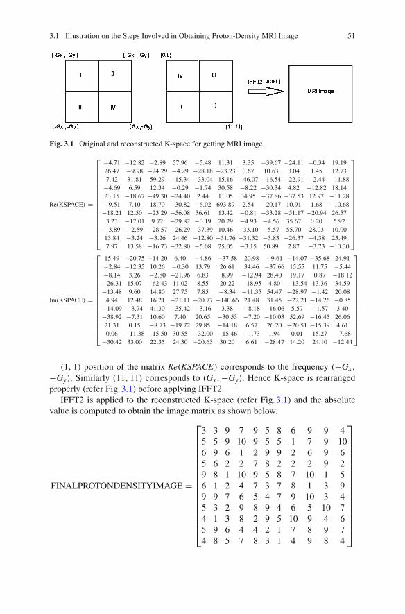
3.1 Illustration on the Steps Involved in Obtaining Proton-Density MRI Image 51
Fig. 3.1 Original and reconstructed K-space for getting MRI image
Re(KSPACE) =
⎡⎢⎢⎢⎢⎢⎢⎢⎢⎢⎢⎢⎢⎢⎢⎢⎢⎢⎣
−4.71 −12.82 −2.89 57.96 −5.48 11.31 3.35 −39.67 −24.11 −0.34 19.1926.47 −9.98 −24.29 −4.29 −28.18 −23.23 0.67 10.63 3.04 1.45 12.737.42 31.81 59.29 −15.34 −33.04 15.16 −46.07 −16.54 −22.91 −2.44 −11.88
−4.69 6.59 12.34 −0.29 −1.74 30.58 −8.22 −30.34 4.82 −12.82 18.1423.15 −18.67 −49.30 −24.40 2.44 11.05 34.95 −37.86 −37.53 12.97 −11.28−9.51 7.10 18.70 −30.82 −6.02 693.89 2.54 −20.17 10.91 1.68 −10.68−18.21 12.50 −23.29 −56.08 36.61 13.42 −0.81 −33.28 −51.17 −20.94 26.57
3.23 −17.01 9.72 −29.82 −0.19 20.29 −4.93 −4.56 35.67 0.20 5.92−3.89 −2.59 −28.57 −26.29 −37.39 10.46 −33.10 −5.57 55.70 28.03 10.0013.84 −3.24 −3.26 24.46 −12.80 −31.76 −31.32 −3.83 −26.37 −4.38 25.497.97 13.58 −16.73 −32.80 −5.08 25.05 −3.15 50.89 2.87 −3.73 −10.30
⎤⎥⎥⎥⎥⎥⎥⎥⎥⎥⎥⎥⎥⎥⎥⎥⎥⎥⎦
Im(KSPACE) =
⎡⎢⎢⎢⎢⎢⎢⎢⎢⎢⎢⎢⎢⎢⎢⎢⎢⎢⎣
15.49 −20.75 −14.20 6.40 −4.86 −37.58 20.98 −9.61 −14.07 −35.68 24.91−2.84 −12.35 10.26 −0.30 13.79 26.61 34.46 −37.66 15.55 11.75 −5.44−8.14 3.26 −2.80 −21.96 6.83 8.99 −12.94 28.40 19.17 0.87 −18.12−26.31 15.07 −62.43 11.02 8.55 20.22 −18.95 4.80 −13.54 13.36 34.59−13.48 9.60 14.80 27.75 7.85 −8.34 −11.35 54.47 −28.97 −1.42 20.08
4.94 12.48 16.21 −21.11 −20.77 −140.66 21.48 31.45 −22.21 −14.26 −0.85−14.09 −3.74 41.30 −35.42 −3.16 3.38 −8.18 −16.06 5.57 −1.57 3.40−38.92 −7.31 10.60 7.40 20.65 −30.53 −7.20 −10.03 52.69 −16.45 26.0621.31 0.15 −8.73 −19.72 29.85 −14.18 6.57 26.20 −20.51 −15.39 4.610.06 −11.38 −15.50 30.55 −32.00 −15.46 −1.73 1.94 0.01 15.27 −7.68
−30.42 33.00 22.35 24.30 −20.63 30.20 6.61 −28.47 14.20 24.10 −12.44
⎤⎥⎥⎥⎥⎥⎥⎥⎥⎥⎥⎥⎥⎥⎥⎥⎥⎥⎦
(1, 1) position of the matrix Re(KSPACE) corresponds to the frequency (−Gx,
−Gy). Similarly (11, 11) corresponds to (Gx,−Gy). Hence K-space is rearrangedproperly (refer Fig. 3.1) before applying IFFT2.
IFFT2 is applied to the reconstructed K-space (refer Fig. 3.1) and the absolutevalue is computed to obtain the image matrix as shown below.
FINALPROTONDENSITYIMAGE =
⎡⎢⎢⎢⎢⎢⎢⎢⎢⎢⎢⎢⎢⎢⎢⎢⎢⎣
3 3 9 7 9 5 8 6 9 9 45 5 9 10 9 5 5 1 7 9 106 9 6 1 2 9 9 2 6 9 65 6 2 2 7 8 2 2 2 9 29 8 1 10 9 5 8 7 10 1 56 1 2 4 7 3 7 8 1 3 99 9 7 6 5 4 7 9 10 3 45 3 2 9 8 9 4 6 5 10 74 1 3 8 2 9 5 10 9 4 65 9 6 4 4 2 1 7 8 9 74 8 5 7 8 3 1 4 9 8 4
⎤⎥⎥⎥⎥⎥⎥⎥⎥⎥⎥⎥⎥⎥⎥⎥⎥⎦

52 3 Illustrations on MRI Techniques Using Matlab
In this procedure, it is noted that at the time of sampling the K-space, there is nosignificant dephasing experienced by the individual magnetic moments at every pixel.Hence the reconstructed image mainly contributes the proton-density at every pixel. Itis observed from the matrix FINALPROTONDENSITYIMAGE that the pixel valuesare exactly the number of individual magnetic moments (n) at every pixel (x, y). Thistype of MRI imaging technique is known as proton-density MRI imaging.
3.1.1.1 protondensity.m
siz=11;K=0.2; %Initial phaseMxyit=[];gamma=2*pi*42.58*(10ˆ6);d1=((10ˆ3)/(11*42.58*(10ˆ6)*0.0000000009));d2=((10ˆ3)/(11*42.58*(10ˆ6)*0.0000000009));B0=1;n=round(rand(siz,siz)*9+1);for x=1:1:siz
for y=1:1:sizfor i=1:1:n(x,y)
k(x,y,i)=rand*2-1;end
endendKSPACE=zeros(11,11);for Gx=-5:1:5;for Gy=-5:1:5;Gy1=Gy/(10ˆ3);%This is to indicate that B0 is high compared with y-gradientGx1=Gx/(10ˆ3);%This is to indicate that B0 is high compared with x-gradientfor x=0:1:siz-1for y=0:1:siz-1for i=1:1:n(x+1,y+1)phi1=k(x+1,y+1,i)*0.0000000009*2*pi;%The magnetic moments after applying y-gradient for the duration of%0.0000000009temp1(x+1,y+1,i)=exp(-j*((B0*gamma+gamma*y*d2*Gy1)*0.0000000009-phi1+K));%The magnetic moments after applying x-gradient for the duration of%0.0000000009 after applying the y-gradient for the duration of%0.0000000009phi2=k(x+1,y+1,i)*0.0000000009*2*pi;temp2(x+1,y+1,i)=exp(-j*((B0*gamma+d2*gamma*y*Gy1)*0.0000000009-phi1+K))...*exp(-j*((B0*gamma-gamma*d1*x*Gx1)*0.0000000009-phi2));%The magnetic moments after applying x-gradient for the duration of%0.0000000018 after applying the y-gradient for the duration of%0.0000000009 and negative x-gradient for the duration of 0.0000000009phi3=k(x+1,y+1,i)*0.0000000018*2*pi;temp3(x+1,y+1,i)=exp(-j*((B0*gamma+gamma*d2*y*Gy1)*0.0000000009-phi1+K))...*exp(-j*((B0*gamma-gamma*d1*x*Gx1)*0.0000000009-phi2))*...exp(-j*((B0*gamma+gamma*d1*x*Gx1)*0.0000000018-phi3));endendend
for x=0:1:siz-1for y=0:1:siz-1
for i=1:1:n(x+1,y+1)

3.1 Illustration on the Steps Involved in Obtaining Proton-Density MRI Image 53
KSPACE(Gx+6,Gy+6)=KSPACE(Gx+6,Gy+6)+temp3(x+1,y+1,i);endend
endendend
KSPACEREARRANGED=KSPACE(6:1:11,6:1:11);KSPACEREARRANGED=[KSPACEREARRANGED KSPACE(6:1:11,1:1:5)];KSPACEREARRANGED=[KSPACEREARRANGED; KSPACE(1:1:5,6:1:11) KSPACE(1:1:5,1:1:5) ];RECONSTRUCTED=ifft2(KSPACEREARRANGED)%Hence the measured image is the proton density image.
3.2 Illustrtion on the Steps Involved in Obtaining the T2 MRIImage Using Cartesian Scanning
Let the image slice be represented as the matrix with the values filled up with proton-density (number of individual magnetic moments available at every pixel) is asfollows.
n =
⎡⎢⎢⎢⎢⎢⎢⎢⎢⎢⎢⎢⎢⎢⎢⎢⎢⎣
3 5 9 3 7 4 7 2 10 3 38 5 5 3 9 1 6 2 9 4 98 3 9 4 2 3 6 5 3 6 63 8 4 9 7 6 4 7 6 8 97 8 7 6 2 6 8 7 8 5 72 9 6 8 7 3 4 7 6 6 37 6 2 4 7 7 7 1 7 2 24 3 5 5 1 2 9 2 6 3 67 6 9 10 8 9 4 8 8 4 54 3 1 2 10 2 8 9 2 5 77 5 4 2 5 4 8 8 5 3 8
⎤⎥⎥⎥⎥⎥⎥⎥⎥⎥⎥⎥⎥⎥⎥⎥⎥⎦
Every magnetic moments at every pixel are assumed to be identical (magnitude andphase) at t = 0. Initial phase of every individual magnetic moments are assumedto be identically equal to K = 0.2. Individual magnetic moments of every pixelundergoes phase change, which varies linearly as 2πk(x, y, i)t, where k(x, y, i) isthe linear phase constant associated with ith magnetic moment at the position (x, y).Phase constants of the individual magnetic moments at every pixel are illustrated inthe Fig. 3.2. Every subplot of the Fig. 3.2 belongs to the individual pixel. For instant(1, 1) subplot corresponds to (1, 1) pixel. The phase constants associated with thethree (note that n(1, 1) = 3) individual magnetic moments at the position (1, 1) isshown as the three stems in the subplot (1, 1). The following steps are followed toobtain T2 image.
1. Apply Gy gradient for the duration of 0.1.2. Apply Gx gradient for the duration of 0.1.

54 3 Illustrations on MRI Techniques Using Matlab
Fig. 3.2 Illustration of the phase constants of the individual magnetic moments at every pixel ofthe image slice of size 11 × 11 (refer Sect. 3.2)
3. Apply 180◦ pulse and allow the magnetic moment to dephase for 0.3. During thisphase, after the time duration of 0.2, there exists the momentary peak occur in theresultant magnitude of the magnetic moment of every pixel. This is called spinecho (refer Sect. 3.2.2). Usually the transverse components reduces drasticallydue to factors other than the spin–spin relaxation. The transverse componentbecomes almost zero before the hardware perform the procedure to capture theMRI signal. But spin echo guarantees the availability of the signal, so that thehardware can capture the required signal.
4. Apply Gx gradient for the duration of 0.2. During this period, there is the cancel-lation of phase introduced due to the Gx component. This is known as Gradientecho. This helps to synchronize the hardware to sample at the particular sampletime to choose the proper position in the K-space. This is similar to the one usedin proton-density MRI image.
5. Sample the real and imaginary component of the signal s(t) to obtain the sampleof the K-space at (Gx,−Gy).
6. Proper scaling factor is used so that the final basis (to perform IFFT2) look like
the standard form e−j2πxGx
11 e−j2πyGy
11 . This is the process of discretization.7. The above steps are repeated for the complete scan in the K-space. For every
time, we have to wait for the longitudinal component to reach maximum beforeapplying 90◦ RF pulse. (This is illustrated by repeating the steps 1–5 by varyingthe values of Gx and Gy ranging from −5 to 5 with the interval of 1).
The obtained K-space is viewed as the function of Gx and G′y = −Gy. The K-
space is rearranged and are subjected to IFFT2 to obtain the MRI image f (x,−y)
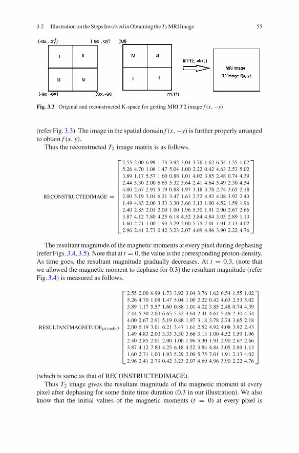
3.2 Illustration on the Steps Involved in Obtaining the T2 MRI Image 55
Fig. 3.3 Original and reconstructed K-space for getting MRI T2 image f (x,−y)
(refer Fig. 3.3). The image in the spatial domain f (x,−y) is further properly arrangedto obtain f (x, y).
Thus the reconstructed T2 image matrix is as follows.
RECONSTRUCTEDIMAGE =
⎡⎢⎢⎢⎢⎢⎢⎢⎢⎢⎢⎢⎢⎣
2.55 2.00 6.99 1.73 3.92 3.04 3.76 1.62 6.54 1.55 1.025.26 4.70 1.08 1.47 5.04 1.00 2.22 0.42 4.63 2.53 5.023.89 1.17 5.57 1.60 0.88 1.01 4.02 3.85 2.48 0.74 4.392.44 5.30 2.00 6.65 5.32 3.64 2.41 4.64 5.49 2.30 4.544.00 2.67 2.91 5.19 0.88 1.97 3.18 3.78 2.74 3.65 2.182.00 5.19 3.01 6.21 3.47 1.61 2.52 4.92 4.08 3.92 2.431.49 4.83 2.00 3.33 3.30 3.66 3.13 1.00 4.52 1.59 1.962.40 2.85 2.01 2.00 1.00 1.96 5.30 1.91 2.90 2.67 2.663.87 4.12 7.80 4.25 6.18 4.52 3.84 4.84 3.05 2.89 1.131.60 2.71 1.00 1.93 5.29 2.00 5.75 7.01 1.91 2.13 4.022.96 2.41 2.73 0.42 3.23 2.07 4.69 4.96 3.90 2.22 4.76
⎤⎥⎥⎥⎥⎥⎥⎥⎥⎥⎥⎥⎥⎦
The resultant magnitude of the magnetic moments at every pixel during dephasing(refer Figs. 3.4, 3.5). Note that at t = 0, the value is the corresponding proton-density.As time goes, the resultant magnitude gradually decreases. At t = 0.3, (note thatwe allowed the magnetic moment to dephase for 0.3) the resultant magnitude (referFig. 3.4) is measured as follows.
RESULTANTMAGNITUDEat t=0.3
⎡⎢⎢⎢⎢⎢⎢⎢⎢⎢⎢⎢⎢⎣
2.55 2.00 6.99 1.73 3.92 3.04 3.76 1.62 6.54 1.55 1.025.26 4.70 1.08 1.47 5.04 1.00 2.22 0.42 4.63 2.53 5.023.89 1.17 5.57 1.60 0.88 1.01 4.02 3.85 2.48 0.74 4.392.44 5.30 2.00 6.65 5.32 3.64 2.41 4.64 5.49 2.30 4.544.00 2.67 2.91 5.19 0.88 1.97 3.18 3.78 2.74 3.65 2.182.00 5.19 3.01 6.21 3.47 1.61 2.52 4.92 4.08 3.92 2.431.49 4.83 2.00 3.33 3.30 3.66 3.13 1.00 4.52 1.59 1.962.40 2.85 2.01 2.00 1.00 1.96 5.30 1.91 2.90 2.67 2.663.87 4.12 7.80 4.25 6.18 4.52 3.84 4.84 3.05 2.89 1.131.60 2.71 1.00 1.93 5.29 2.00 5.75 7.01 1.91 2.13 4.022.96 2.41 2.73 0.42 3.23 2.07 4.69 4.96 3.90 2.22 4.76
⎤⎥⎥⎥⎥⎥⎥⎥⎥⎥⎥⎥⎥⎦
(which is same as that of RECONSTRUCTEDIMAGE).Thus T2 image gives the resultant magnitude of the magnetic moment at every
pixel after dephasing for some finite time duration (0.3 in our illustration). We alsoknow that the initial values of the magnetic moments (t = 0) at every pixel is
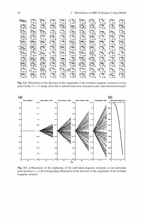
56 3 Illustrations on MRI Techniques Using Matlab
Fig. 3.4 Illustration of the decrease in the magnitude of the resultant magnetic moment at everypixel (of the 11 × 11 image slice) due to natural transverse relaxation (spin–spin interaction based)
Fig. 3.5 a Illustration of the dephasing of the individual magnetic moments at one particularpixel position (x, y); b corresponding illustration of the decrease in the magnitude of the resultantmagnetic moment

3.2 Illustration on the Steps Involved in Obtaining the T2 MRI Image 57
measured using proton-density image. Let the resultant magnitude of the magneticmoment of the pixel (x, y) at t = 0 and at t = 0.3 be represented as K(x, y)0 and
K(x, y)0.3 respectively. They are related as K(x, y)0.3 = K(x, y)0e−0.3
T2(x,y) . Hence
T2(x, y) = 0.3 ∗ loge
(K(x, y)0.3
K(x, y)0
)(3.1)
Thus T2 image is obtained as follows.
FINALT2IMAGE =
⎡⎢⎢⎢⎢⎢⎢⎢⎢⎢⎢⎢⎢⎢⎢⎢⎢⎢⎣
0.16 0.92 0.2527 0.5505 0.5798 0.2744 0.6215 0.2107 0.4246 0.6604 1.07880.42 0.06 1.5325 0.7133 0.5798 0 0.9943 1.5606 0.6647 0.4581 0.58380.72 0.94 0.4798 0.9163 0.8210 1.0887 0.4005 0.2614 0.1904 2.0929 0.31240.21 0.41 0.6931 0.3026 0.2744 0.4998 0.5067 0.4112 0.0888 1.2465 0.68430.56 1.0974 0.8778 0.1450 0.8210 1.1137 0.9226 0.6162 1.0715 0.3147 1.1666
0 0.5505 0.6898 0.2533 0.7018 0.6224 0.4620 0.3526 0.3857 0.4257 0.21071.55 0.2169 0 0.1833 0.7520 0.6484 0.8049 0 0.4374 0.2294 0.02020.51 0.0513 0.9113 0.9163 0 0.0202 0.5295 0.0460 0.7270 0.1165 0.81340.59 0.3759 0.1431 0.8557 0.2581 0.6887 0.0408 0.5025 0.9643 0.3250 1.48720.92 0.1017 0 0.0356 0.6368 0 0.3302 0.2499 0.0460 0.8533 0.55460.86 0.7298 0.3820 1.5606 0.4370 0.6587 0.5340 0.4780 0.2485 0.3011 0.5192
⎤⎥⎥⎥⎥⎥⎥⎥⎥⎥⎥⎥⎥⎥⎥⎥⎥⎥⎦
3.2.1 Note to the Fig. 3.4
1. The initial magnitude of the resultant magnetic moment gives the proton-densityof the particular pixel. This leads to proton-density image.
2. The rate at which the resultant magnetic moment is decreasing gives the timeconstant T2, which leads to T2 image.
3.2.1.1 t2.m
siz=11;K=0.2; %Initial phaseMxyit=[];gamma=2*pi*42.58*(10ˆ6);d1=((10ˆ3)/(11*42.58*10ˆ6*0.1));d2=((10ˆ3)/(11*42.58*10ˆ6*0.1));B0=1;n=round(rand(siz,siz)*9+1);%n=ones(siz,siz)*10;for x=1:1:siz
for y=1:1:sizfor i=1:1:n(x,y)
k(x,y,i)=rand*2-1;end
endendKSPACE=zeros(11,11);for Gx=-5:1:5;for Gy=-5:1:5;

58 3 Illustrations on MRI Techniques Using Matlab
Gx1=Gx/(10ˆ3);Gy1=Gy/(10ˆ3);for x=0:1:siz-1for y=0:1:siz-1for i=1:1:n(x+1,y+1)phi1=k(x+1,y+1,i)*0.1*2*pi;%The magnetic moments after applying positive y-gradient for the duration of%0.1temp1(x+1,y+1,i)=exp(-j*((B0*gamma+gamma*y*d2*Gy1)*0.1-phi1+K));%The magnetic moments after applying negative x-gradient for the duration of%0.1 after applying the y-gradient for the duration of 0.1
phi2=k(x+1,y+1,i)*0.1*2*pi;temp2(x+1,y+1,i)=exp(-j*((B0*gamma+d2*gamma*y*Gy1)*0.1-phi1+K))...*exp(-j*((B0*gamma+gamma*d1*x*Gx1)*0.1-phi2));%Apply 180 degree phase shift and allow it to dephase for 0.3 durationphi3=k(x+1,y+1,i)*0.3*2*pi;temp3(x+1,y+1,i)=exp(j*((B0*gamma+gamma*d2*y*Gy1)*0.1-phi1+K))...*exp(j*((B0*gamma+gamma*d1*x*Gx1)*0.1-phi2))*...exp(-j*((B0*gamma)*0.3-phi3));
%apply positive x-gradient for readout for the duration of 0.2
phi4=k(x+1,y+1,i)*0.2*2*pi;temp3(x+1,y+1,i)=exp(j*((B0*gamma+gamma*d2*y*Gy1)*0.1-phi1+K))...*exp(j*((B0*gamma+gamma*d1*x*Gx1)*0.1-phi2))*...exp(-j*((B0*gamma)*0.3-phi3))*exp(-j*((B0*gamma+gamma*d1*x*Gx1)*0.2-phi4));
endendend
for x=0:1:siz-1for y=0:1:siz-1
for i=1:1:n(x+1,y+1)KSPACE(Gx+6,Gy+6)=KSPACE(Gx+6,Gy+6)+temp3(x+1,y+1,i);end
endendendendKSPACEREARRANGED=KSPACE(6:1:11,6:1:11);KSPACEREARRANGED=[KSPACEREARRANGED KSPACE(6:1:11,1:1:5)];KSPACEREARRANGED=[KSPACEREARRANGED; KSPACE(1:1:5,6:1:11) KSPACE(1:1:5,1:1:5) ];RECONSTRUCTED=abs(ifft2(KSPACEREARRANGED));%But note that what we reconstructed is f(x,-y) and not f(x,y).save T2DATA n kFINALRECONSIMAGE=zeros(11,11);FINALRECONSIMAGE(:,1)=RECONSTRUCTED(:,1);for p=1:1:11
for q=2:1:11FINALRECONSIMAGE(p,q)=RECONSTRUCTED(p,13-q);
endend

3.2 Illustration on the Steps Involved in Obtaining the T2 MRI Image 59
3.2.1.2 Relaxation.m
load T2DATAvector=0for x=1:1:11
for y=1:1:11MAG{x,y}=[];for t=0:0.01:0.3
vector=0;for i=1:1:n(x,y)
phi=k(x,y,i)*t*2*pi;vector=vector+exp(-j*phi);
endMAG{x,y}=[MAG{x,y} abs(vector)];
endend
endfiguresub=1;for x=1:1:11
for y=1:1:11subplot(11,11,sub)%plot(MAG{x,y}/max(MAG{x,y}))plot(MAG{x,y})sub=sub+1;COLLECTION(x,y)=MAG{x,y}(length(MAG{x,y}));
endend
3.2.1.3 Dephasing.m
%Concept of dephasingMAG=[];t=0:0.01:1;vectorsum=0;k=rand(1,100)*2-1;snap=1;for t=0:0.01:0.04vectorsum=0;for i=1:1:100phi=k(i)*t*2*pi;subplot(1,6,snap)hold onplot([0 cos(phi)],[0 -sin(phi)],’k’)title(strcat(’Time instant’,num2str(t)))vectorsum=vectorsum+exp(-j*phi);endMAG=[MAG vectorsum];snap=snap+1;endsubplot(1,6,snap)plot(abs(MAG),’k’)title(’Resultant magnitude versus time’)xlabel(’Time’)

60 3 Illustrations on MRI Techniques Using Matlab
3.2.2 Momentary Peak Due to Spin Echo
The following experiment demonstrate the momentary peak of the resultant mag-nitude at every pixel achieved after applying 180◦ pulse. This is due to rephasing.This is called spin echo. Spin echo helps to obtain the significant signal for a whileso that the hardware can capture the required signal during dephasing. The experi-ment involves obtaining the spatial domain image at three different time instancesas described below.Time instant: 0.2
1. Initialize k and n.2. Apply Gy gradient for the duration of 0.1.3. Apply the read-out Gx gradient for the duration of 0.1.4. Sample the value at the end of read-out duration.5. Sample value corresponds to Gx, Gy.6. Note that the resultant magnitude at every pixel (at time instant t = 0.2) corre-
sponds to the values obtained after dephasing for the duration of 0.2.
Time instant: 0.4
1. Initialize k and n (same as that of the one used in the case of time instant t = 0.2).2. Apply Gy gradient for the duration of 0.1.3. Apply Gx gradient for the duration of 0.1.4. Apply 180◦ RF pulse.5. Apply read-out Gx gradient for the duration of 0.2.6. Sample the value at the end of read-out duration.7. Sample value corresponds to Gx,−Gy.8. Note that the resultant magnitude at every pixel (at time instant t = 0.4) corre-
sponds to the values obtained after rephasing for the duration of 0.2 (obtainedduring read-out phase), after the time instant t = 0.2.
9. This is the spin–echo instant at which momentary peak has occurred.
Time instant: 0.5
1. Initialize k and n (same as that of the one used in the case of time instant t = 0.2).2. Apply Gy gradient for the duration of 0.1.3. Apply Gx gradient for the duration of 0.1.4. Apply 180◦ RF pulse.5. Allow relaxation explicitly for the duration of 0.1. This helps to cancel out partially
the phase introduced in steps 1 and 2. This step acts as the rephasing stage.6. Apply read-out Gx gradient for the duration of 0.2. During this phase, the first
0.1 s acts as the rephasing stage to obtain the echo at 0.4. The next 0.1 s acts asthe dephasing stage.
7. Sample the value at the end of read-out duration.8. Sample value corresponds to Gx,−Gy.

3.2 Illustration on the Steps Involved in Obtaining the T2 MRI Image 61
9. Thus the resultant magnitude at every pixel (at time instant t = 0.5) correspondsto the values obtained after dephasing of the resultant magnetic moment for theduration of 0.1. This is obviously lesser than the value at time instant t = 0.4
The spatial matrix at three different time instances (described in the Sect. 3.2.2)are given below.
S0.2 =
⎡⎢⎢⎢⎢⎢⎢⎢⎢⎢⎢⎢⎢⎢⎢⎢⎢⎣
1.00 5.84 6.11 2.96 2.79 2.54 7.93 6.99 7.59 1.42 3.421.00 5.95 3.56 2.05 7.00 5.67 3.33 1.34 9.14 1.00 6.022.29 4.33 5.73 4.04 6.44 4.00 1.65 5.33 6.53 1.87 4.683.74 3.86 1.89 7.07 6.67 4.16 3.63 2.86 6.67 5.09 3.756.69 3.26 2.86 3.18 3.72 6.90 5.76 6.66 4.41 1.81 1.456.06 2.00 3.53 4.44 3.94 2.97 3.45 4.92 1.00 7.98 4.586.16 4.48 1.97 3.96 3.87 6.15 5.39 7.60 6.42 3.03 4.045.40 4.84 3.27 3.95 5.90 6.34 5.56 5.78 3.33 2.50 5.278.72 6.32 1.00 5.23 3.13 4.72 1.00 1.84 5.00 3.89 6.112.18 2.98 2.55 3.61 2.00 2.57 1.86 2.00 7.09 1.94 1.004.24 2.31 2.45 5.02 8.00 6.04 4.45 2.00 2.09 2.41 1.55
⎤⎥⎥⎥⎥⎥⎥⎥⎥⎥⎥⎥⎥⎥⎥⎥⎥⎦
S0.4 =
⎡⎢⎢⎢⎢⎢⎢⎢⎢⎢⎢⎢⎢⎢⎢⎢⎢⎣
2.00 6.00 7.00 4.00 3.00 3.00 9.00 9.00 10.00 2.00 4.001.00 7.00 4.00 3.00 9.00 8.00 4.00 2.00 10.00 1.00 7.003.00 6.00 7.00 5.00 8.00 5.00 2.00 7.00 9.00 3.00 6.004.00 4.00 2.00 10.00 9.00 5.00 5.00 4.00 8.00 8.00 4.008.00 4.00 5.00 4.00 5.00 9.00 8.00 8.00 6.00 2.00 2.009.00 2.00 4.00 5.00 6.00 4.00 4.00 6.00 1.00 9.00 6.008.00 6.00 2.00 4.00 5.00 8.00 8.00 10.00 8.00 4.00 6.006.00 6.00 4.00 4.00 8.00 8.00 7.00 7.00 5.00 3.00 8.00
10.00 8.00 1.00 6.00 4.00 6.00 1.00 3.00 5.00 4.00 9.003.00 3.00 4.00 5.00 2.00 4.00 2.00 2.00 9.00 2.00 1.006.00 3.00 3.00 6.00 9.00 8.00 6.00 2.00 3.00 3.00 2.00
⎤⎥⎥⎥⎥⎥⎥⎥⎥⎥⎥⎥⎥⎥⎥⎥⎥⎦
S0.5 =
⎡⎢⎢⎢⎢⎢⎢⎢⎢⎢⎢⎢⎢⎢⎢⎢⎢⎣
1.73 5.96 6.77 3.72 2.95 2.88 8.72 8.44 9.37 1.85 3.851.00 6.71 3.89 2.74 8.47 7.37 3.83 1.88 9.78 1.00 6.752.81 5.56 6.66 4.75 7.59 4.74 1.91 6.55 8.34 2.69 5.653.94 3.96 1.97 9.23 8.36 4.78 4.63 3.68 7.65 7.22 3.94
7.650 3.80 4.42 3.78 4.67 8.45 7.40 7.65 5.58 1.95 1.868.21 2.00 3.88 4.85 5.46 3.73 3.86 5.72 1.00 8.74 5.607.51 5.60 2.00 3.99 4.71 7.52 7.30 9.35 7.58 3.75 5.485.85 5.70 3.80 3.99 7.45 7.55 6.63 6.67 4.56 2.87 7.279.66 7.55 1.00 5.80 3.77 5.66 1.00 2.68 5.00 3.97 8.222.78 3.00 3.58 4.64 2.00 3.61 1.96 2.00 8.46 1.98 1.005.53 2.82 2.86 5.73 8.72 7.47 5.59 2.00 2.76 2.85 1.88
⎤⎥⎥⎥⎥⎥⎥⎥⎥⎥⎥⎥⎥⎥⎥⎥⎥⎦
Note that the elements of the matrix S0.4 corresponds to the local maxima occurreddue to rephasing (spin echo).

62 3 Illustrations on MRI Techniques Using Matlab
3.2.2.1 Spinechodemonstration.m
siz=11;K=0.2; %Initial phaseMxyit=[];gamma=2*pi*42.58*(10ˆ6);d1=((10ˆ3)/(11*42.58*10ˆ6*0.1));d2=((10ˆ3)/(11*42.58*10ˆ6*0.1));B0=1;n=round(rand(siz,siz)*9+1);for x=1:1:siz
for y=1:1:sizfor i=1:1:n(x,y)
k(x,y,i)=rand*2-1;end
endend
KSPACE=zeros(11,11);for i=1:1:3KKSPACE{i}=zeros(11,11);endfor Gx=-5:1:5;for Gy=-5:1:5;Gx1=Gx/(10ˆ3);Gy1=Gy/(10ˆ3);for x=0:1:siz-1for y=0:1:siz-1for i=1:1:n(x+1,y+1)phi1=k(x+1,y+1,i)*0.1*2*pi;%The magnetic moments after applying positive y-gradient for the duration of%0.1temp1(x+1,y+1,i)=exp(-j*((B0*gamma+gamma*y*d2*Gy1)*0.1-phi1+K));%Case 1:%At time instant=0.2 (refer section 3.2.2)phi2=k(x+1,y+1,i)*0.1*2*pi;temp2(x+1,y+1,i)=exp(-j*((B0*gamma+d2*gamma*y*Gy1)*0.1-phi1+K))...*exp(-j*((B0*gamma+gamma*d1*x*Gx1)*0.1-phi2));
%Case 2:%At time instant=0.4 (refer section 3.2.2)
phi3=k(x+1,y+1,i)*0.2*2*pi;temp3(x+1,y+1,i)=exp(j*((B0*gamma+gamma*d2*y*Gy1)*0.1-phi1+K))...*exp(j*((B0*gamma+gamma*d1*x*Gx1)*0.1-phi2))*...exp(-j*((B0*gamma+gamma*d1*x*Gx1)*0.2-phi3));
%Case 3:%At time instant=0.8 (refer section 3.2.2)phi4=k(x+1,y+1,i)*0.1*2*pi;phi5=k(x+1,y+1,i)*0.2*2*pi;temp4(x+1,y+1,i)=exp(j*((B0*gamma+gamma*d2*y*Gy1)*0.1-phi1+K))...*exp(j*((B0*gamma+gamma*d1*x*Gx1)*0.1-phi2))*...exp(-j*((B0*gamma)*0.1-phi4))*exp(-j*((B0*gamma+gamma*d1*x*Gx1)*0.2-phi5));endendend
for x=0:1:siz-1for y=0:1:siz-1

3.2 Illustration on the Steps Involved in Obtaining the T2 MRI Image 63
for i=1:1:n(x+1,y+1)KKSPACE{1}(Gx+6,Gy+6)=KKSPACE{1}(Gx+6,Gy+6)+temp2(x+1,y+1,i);KKSPACE{2}(Gx+6,Gy+6)=KKSPACE{2}(Gx+6,Gy+6)+temp3(x+1,y+1,i);KKSPACE{3}(Gx+6,Gy+6)=KKSPACE{3}(Gx+6,Gy+6)+temp4(x+1,y+1,i);
endend
endendend
KSPACE=KKSPACE{1};KSPACEREARRANGED=KSPACE(6:1:11,6:1:11);KSPACEREARRANGED=[KSPACEREARRANGED KSPACE(6:1:11,1:1:5)];KSPACEREARRANGED=[KSPACEREARRANGED; KSPACE(1:1:5,6:1:11) KSPACE(1:1:5,1:1:5) ];SPINECHO{1}=abs(ifft2(KSPACEREARRANGED));%Note that what we have reconstructed f(x,y)
for i=2:1:3KSPACE=KKSPACE{i};KSPACEREARRANGED=KSPACE(6:1:11,6:1:11);KSPACEREARRANGED=[KSPACEREARRANGED KSPACE(6:1:11,1:1:5)];KSPACEREARRANGED=[KSPACEREARRANGED; KSPACE(1:1:5,6:1:11) KSPACE(1:1:5,1:1:5) ];RECONSTRUCTED=abs(ifft2(KSPACEREARRANGED));%But note that what we reconstructed is f(x,-y) and not f(x,y).%f(x,y) is reconstructed as follows.FINALRECONSIMAGE=zeros(11,11);FINALRECONSIMAGE(:,1)=RECONSTRUCTED(:,1);for p=1:1:11
for q=2:1:11FINALRECONSIMAGE(p,q)=RECONSTRUCTED(p,13-q);
endendSPINECHO{i}=FINALRECONSIMAGE;end
3.3 Illustration on the Steps Involved in Obtaining the T2 MRIImage Using Polar Scanning
1. Initialize n and k.2. Apply Gx and Gy gradient simultaneously for the duration of 0.1 corresponding
to the controlling parameter r and θ i.e. Gx = rcos(θ) and Gy = rsin(θ).
3. Apply 180◦ pulse for the duration of 0.3.4. Allow the resultant magnetic moment to dephase for the duration of 0.3.5. Apply the Gx and Gy gradient simultaneously for the duration of 0.2 as the read-
out phase. Sample the value at the end of the read-out phase. This correspondsto Gx = rcos(θ) and Gy = rsin(θ).
6. Note that the steps used in this technique are exactly same as that of Cartesianspin–echo based T2 MRI. The difference is, in this case K-space is scanned inthe polar fashion as shown in the Fig. 3.6.
7. This is repeated for specific range of r (depends upon on the resolution requiredfor the image slice) and θ ranges from 0 to π .
8. K-space data F(Gx, Gy) = F(rcos(θ), rsin(θ)) is rewritten as G(r, θ).

64 3 Illustrations on MRI Techniques Using Matlab
Fig. 3.6 a Illustrating the order in which the K-space is scanned; b sample polar scanned K-space
9. Apply inverse fourier transformation in polar form to obtain f (x, y) (referSect. 3.3.1).
10. For checking the validity of reconstruction from polar data, k is chosen as zeromatrix (No dephasing) for illustration. This helps to obtain proton-density image(n-matrix) as the reconstructed image.
3.3.1 Reconstructing f (x, y) from G(r, θ)
There are two major techniques to obtain f (x, y) from G(r, θ) namely back-projection technique and the interpolation technique as described below. Theinterpolation technique is used for illustration purpose.
3.3.1.1 Back-Projection Technique
The generalized formula to reconstruct f (x, y) from G(r, θ) is as shown below.
f (x, y) =π∫
−π
∞∫
0
G(r, θ) expj2π(xcosθ+ysinθ)r |J|drdθ (3.2)
1. It it noted G(r, θ) is the fourier transformation of the radon transformation R(l, θ)
for the specific constant θ .2. It is possible to get back f (x, y) by getting R(l, θ) using inverse fourier transfor-
mation (refer Sect. 1.2), followed by back-projection technique.
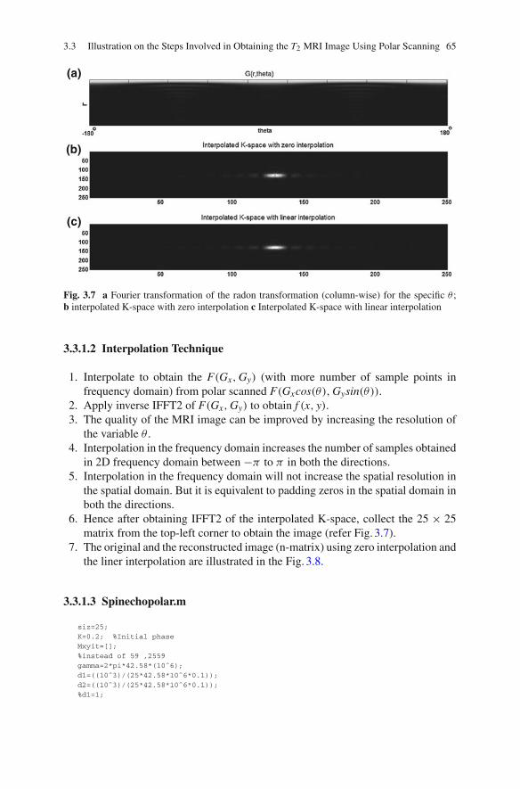
3.3 Illustration on the Steps Involved in Obtaining the T2 MRI Image Using Polar Scanning 65
(a)
(b)
(c)
Fig. 3.7 a Fourier transformation of the radon transformation (column-wise) for the specific θ ;b interpolated K-space with zero interpolation c Interpolated K-space with linear interpolation
3.3.1.2 Interpolation Technique
1. Interpolate to obtain the F(Gx, Gy) (with more number of sample points infrequency domain) from polar scanned F(Gxcos(θ), Gysin(θ)).
2. Apply inverse IFFT2 of F(Gx, Gy) to obtain f (x, y).3. The quality of the MRI image can be improved by increasing the resolution of
the variable θ .4. Interpolation in the frequency domain increases the number of samples obtained
in 2D frequency domain between −π to π in both the directions.5. Interpolation in the frequency domain will not increase the spatial resolution in
the spatial domain. But it is equivalent to padding zeros in the spatial domain inboth the directions.
6. Hence after obtaining IFFT2 of the interpolated K-space, collect the 25 × 25matrix from the top-left corner to obtain the image (refer Fig. 3.7).
7. The original and the reconstructed image (n-matrix) using zero interpolation andthe liner interpolation are illustrated in the Fig. 3.8.
3.3.1.3 Spinechopolar.m
siz=25;
K=0.2; %Initial phase
Mxyit=[];
%instead of 59 ,2559
gamma=2*pi*42.58*(10ˆ6);
d1=((10ˆ3)/(25*42.58*10ˆ6*0.1));
d2=((10ˆ3)/(25*42.58*10ˆ6*0.1));
%d1=1;

66 3 Illustrations on MRI Techniques Using Matlab
Fig. 3.8 Illustration of the original and the reconstructed spatial domain (proton-density) from thepolar scanned K-space G(r, θ)
%d2=1;
B0=1;
n=ones(3,25)*2;
for i=1:1:10
n=[n;ones(1,25)*i];
end
for i=10:-1:1
n=[n;ones(1,25)*i];
end
n=[n;ones(2,25)*1];
POS=[];
for x=1:1:siz
for y=1:1:siz
for i=1:1:n(x,y)
% k(x,y,i)=rand*2-1; %With dephasing
k(x,y,i)=0; %Just to check the validity of the program
end
end
end
KSPACE=zeros(101,180);
for r=0:(13/100):13
r1=round((r)*(100/13)+1);
for theta=-pi:(2*pi)/179:pi
theta1=round((theta+pi)*(179/(2*pi))+1);
Gx=r*cos(theta) ;
Gy=r*sin(theta);
Gx1=Gx/(10ˆ3);
Gy1=Gy/(10ˆ3);
POS=[POS;
Gx Gy];
temp=0;
for x=0:1:24
for y=0:1:24
for i=1:1:n(x+1,y+1)
phi1=k(x+1,y+1,i)*0.1*2*pi;
%x-Gradient and y-Gradient are applied simultaneously for the duration of
%0.1

3.3 Illustration on the Steps Involved in Obtaining the T2 MRI Image Using Polar Scanning 67
temp1(x+1,y+1,i)=exp(-j*((B0*gamma+gamma*y*d2*Gy1)*0.1-phi1+K))...
*exp(-j*((B0*gamma+gamma*x*d1*Gx1)*0.1-phi1+K));
%Apply 180 degree phase shift and allow it to dephase for 0.3 duration
phi2=k(x+1,y+1,i)*0.3*2*pi;
temp2(x+1,y+1,i)=exp(j*((B0*gamma+gamma*y*d2*Gy1)*0.1-phi1+K))*...
exp(j*((B0*gamma+gamma*x*d1*Gx1)*0.1-phi1+K))*...
exp(-j*((B0*gamma)*0.3-phi2));
%Positive x-Gradient and y-Gradient are applied simultaneously for the duration of
%0.2 as the read-out time duphase. At the end of the read-out phase,the
%k-space is sampled corresponding to (r,theta)
phi3=k(x+1,y+1,i)*0.2*2*pi;
temp3(x+1,y+1,i)=exp(j*((B0*gamma+gamma*y*d2*Gy1)*0.1-phi1+K))*...
exp(j*((B0*gamma+gamma*x*d1*Gx1)*0.1-phi1+K))*...
exp(-j*((B0*gamma)*0.3-phi2))*exp(-j*((B0*gamma+gamma*y*d2*Gy1)*...
0.2-phi3))*exp(-j*((B0*gamma+gamma*x*d1*Gx1)*0.2-phi3));
end
end
end
for x=0:1:siz-1
for y=0:1:siz-1
for i=1:1:n(x+1,y+1)
KSPACE(r1,theta1)=KSPACE(r1,theta1)+temp3(x+1,y+1,i);
end
end
end
end
end
%Reconstruction using second technique(refer section 2.11.2)
F=KSPACE;
POS=round((POS+14)*10);
%Number of samples in frequency domain is increased as 250x250 from 25x25
%and zero interpolated.
A=zeros(250,250);
r1=1;
theta1=1;
for i=1:1:length(POS)
F(r1,theta1)
A(POS(i,1),POS(i,2))=F(r1,theta1) ;
theta1=theta1+1;
if(theta1==181)
r1=r1+1;
theta1=1;
end
end
figure
A=fftshift(A);
imagesc(abs(A))
C1=abs(ifft2(A));
%Increase the number of samples in frequency domain from 25x25 to 250x250
%and apply Linear interpolation,considering 8 neighbours of every pixel.
B=A;
[p,q]=find(B==0);
C=[zeros(1,250);B;zeros(1,250)];
C=[zeros(252,1) C zeros(252,1)];
p=p+1;q=q+1;
D=C;
for i=1:1:length(p)
vector=[C(p(i)-1,q(i)-1) C(p(i)-1,q(i)+1) C(p(i)+1,q(i)-1) C(p(i)+1,q(i)+1) ...
C(p(i),q(i)-1) C(p(i),q(i)+1) C(p(i)+1,q(i)) C(p(i)+1,q(i))];
D(p(i),q(i))=mean(vector);
end
B=D(2:1:251,2:1:251);

68 3 Illustrations on MRI Techniques Using Matlab
Fig. 3.9 Illustration of the increase in the magnitude of the resultant longitudinal magnetic momentat every pixel (of the 11 × 11 image slice) due to natural longitudinal relaxation (spin–latticeinteraction based)
figure
imagesc(abs(B))
C2=abs(ifft2(B));
figure
colormap(gray)
subplot(3,1,1)
imagesc(n)
title(’Original’)
subplot(3,1,2)
imagesc(C1(1:1:25,1:1:25))
title(’With zero interpolation in frequency domain’)
subplot(3,1,3)
title(’With Linear interpolation in frequency domain’)
imagesc(C2(1:1:25,1:1:25))
3.4 Illustration on the Steps Involved in Obtaining the T1 MRIImage
The following steps are followed to obtain the T1 image.
1. Select the image slice using z-gradient. Apply refocussing gradient to compen-sate the phase introduced due to z-gradient.
2. Apply 90◦ pulse to obtain the transverse component.3. The transverse component at different pixel starts dephasing due to spin–spin
interaction (described by the factor T2(x, y)).
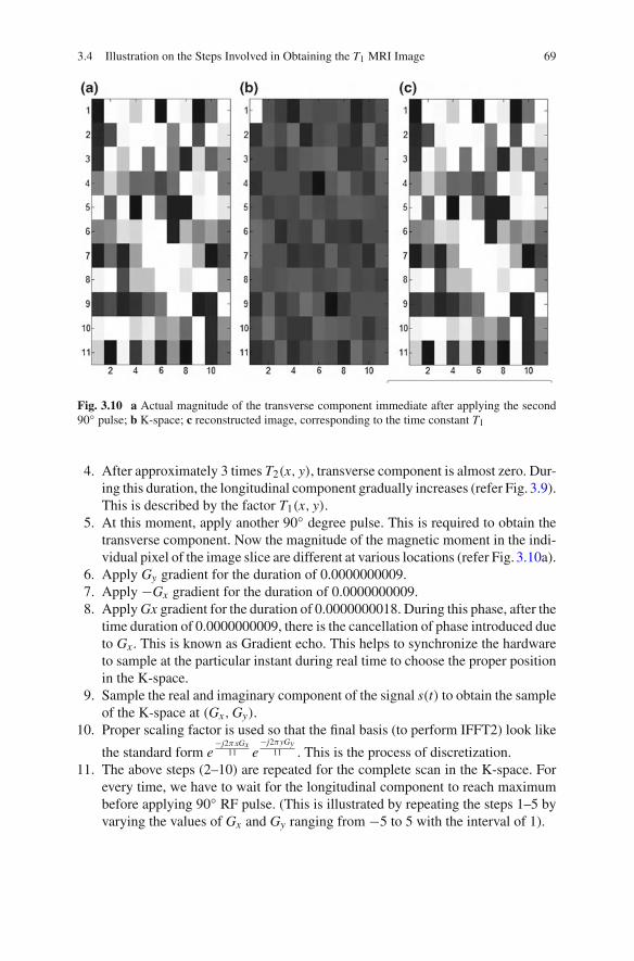
3.4 Illustration on the Steps Involved in Obtaining the T1 MRI Image 69
Fig. 3.10 a Actual magnitude of the transverse component immediate after applying the second90◦ pulse; b K-space; c reconstructed image, corresponding to the time constant T1
4. After approximately 3 times T2(x, y), transverse component is almost zero. Dur-ing this duration, the longitudinal component gradually increases (refer Fig. 3.9).This is described by the factor T1(x, y).
5. At this moment, apply another 90◦ degree pulse. This is required to obtain thetransverse component. Now the magnitude of the magnetic moment in the indi-vidual pixel of the image slice are different at various locations (refer Fig. 3.10a).
6. Apply Gy gradient for the duration of 0.0000000009.7. Apply −Gx gradient for the duration of 0.0000000009.8. Apply Gx gradient for the duration of 0.0000000018. During this phase, after the
time duration of 0.0000000009, there is the cancellation of phase introduced dueto Gx . This is known as Gradient echo. This helps to synchronize the hardwareto sample at the particular instant during real time to choose the proper positionin the K-space.
9. Sample the real and imaginary component of the signal s(t) to obtain the sampleof the K-space at (Gx, Gy).
10. Proper scaling factor is used so that the final basis (to perform IFFT2) look like
the standard form e−j2πxGx
11 e−j2πyGy
11 . This is the process of discretization.11. The above steps (2–10) are repeated for the complete scan in the K-space. For
every time, we have to wait for the longitudinal component to reach maximumbefore applying 90◦ RF pulse. (This is illustrated by repeating the steps 1–5 byvarying the values of Gx and Gy ranging from −5 to 5 with the interval of 1).

70 3 Illustrations on MRI Techniques Using Matlab
12. In the earlier illustrations (T2 and proton-density imaging), we have consideredthe proton-density at every pixel(number of magnetic moments). But in this case,the illustration is done in the macro level at every pixel.
13. The actual magnitude of the transverse component immediate after applying thesecond 90◦ pulse, K-space and the corresponding the reconstructed image areshown in the Fig. 3.10.
3.4.1 t1.m
siz=11;K=0.2; %Initial phasegamma=2*pi*42.58*(10ˆ6);d1=((10ˆ3)/(11*42.58*(10ˆ6)*0.0000000009));d2=((10ˆ3)/(11*42.58*(10ˆ6)*0.0000000009));t1=1;B0=1%Mz(x,y) is the longituidanal component at (x,y).T1=rand(11,11);for tb=0:0.01:1;
t1=t1+1;for x=1:1:11
for y=1:1:11Mz{x,y}(t1)=(1-exp(-tb/T1(x,y)))*B0;
endendendi=1;%snapshotfor x=1:1:11for y=1:1:11subplot(11,11,i)plot(Mz{x,y})i=i+1;endend%At tb=1 (at which the original transverse component due%to dephasing is almost zero),90 degree pulse is again applied.%Now the transverse component at different%pixel in the image slice have different magnitude.for x=1:1:11
for y=1:1:11M(x,y)=Mz{x,y}(101);
endend%M is the magnitude of the individual transverse component at every pixel%immediate after applying the 90 degree pulse (at t=0).
%Sampling the k-space at Gx,Gy.temp1=0;temp2=0;temp3=0;KSPACE=zeros(11,11);for Gx=-5:1:5;for Gy=-5:1:5;Gy1=Gy/(10ˆ3);%This is to indicate that B0 is high compared with y-gradient

3.4 Illustration on the Steps Involved in Obtaining the T1 MRI Image 71
Gx1=Gx/(10ˆ3);%This is to indicate that B0 is high compared with x-gradientfor x=0:1:siz-1for y=0:1:siz-1%The magnetic moments after applying y-gradient for the duration of%0.0000000009temp1=temp1+M(x+1,y+1)*exp(-j*((B0*gamma+gamma*y*d2*Gy1)*0.0000000009+K));%The magnetic moments after applying negative x-gradient for the duration of%0.0000000009 after applying the y-gradient for the duration of%0.0000000009temp2=temp2+M(x+1,y+1)*exp(-j*((B0*gamma+d2*gamma*y*Gy1)*0.0000000009+K))...*exp(-j*((B0*gamma-gamma*d1*x*Gx1)*0.0000000009));%The magnetic moments after applying x-gradient for the duration of%0.0000000018 after applying the y-gradient for the duration of%0.0000000009 and negative x-gradient for the duration of 0.0000000009temp3=temp3+M(x+1,y+1)*exp(-j*((B0*gamma+gamma*d2*y*Gy1)*0.0000000009+K))...*exp(-j*((B0*gamma-gamma*d1*x*Gx1)*0.0000000009))*...exp(-j*((B0*gamma+gamma*d1*x*Gx1)*0.0000000018));endendKSPACE(Gx+6,Gy+6)=temp3;temp1=0;temp2=0;temp3=0;endendKSPACEREARRANGED=KSPACE(6:1:11,6:1:11);KSPACEREARRANGED=[KSPACEREARRANGED KSPACE(6:1:11,1:1:5)];KSPACEREARRANGED=[KSPACEREARRANGED; KSPACE(1:1:5,6:1:11) KSPACE(1:1:5,1:1:5) ];RECONSTRUCTED=ifft2(KSPACEREARRANGED)figuresubplot(1,3,1)colormap(gray)imagesc(M)subplot(1,3,2)colormap(gray)imagesc(log(abs(KSPACEREARRANGED)))subplot(1,3,3)colormap(gray)imagesc(abs(RECONSTRUCTED))

Chapter 4Medical Image Processing
4.1 Summary on the Various Medical Imaging Techniques
1. X-ray image: X-ray is transmitted through the body and are captured on the otherside of the body. The attenuation introduced in the ray helps in obtaining the image.There are different modalities used in X-ray imaging. Example: Angiography,Neuroradiology.
2. Computed Tomography (CT): This is identical to X-ray. But in this case, thesequence of images are captured by rotating the image slice for 180◦ with theresolution of θres degree. This helps to capture the particular slice of the humanbody. Refer Chap. 1 for further details.
3. Magnetic Resonance Imaging (MRI): In this case, human body is exited with thestrong external magnetic field to obtain the resultant magnetic moment at everyvoxel to align in the identical direction. These magnetic moments are disturbedwith the external RF excitation and the transverse component of the magneticmoments are captured. Based on the methodology, MRI is capable of capturingthe characteristics of the proton-density (PD image), spin–spin interaction be-tween the magnetic moments (T2 image), spin–lattice interaction of the magneticmoments (T1 image). Refer Chap. 2 for further details.
4. Ultrasound image: The ultrasound waves are transmitted through the human bodyand the reflected wave (due to reflection and the scattering) is recorded to obtainthe image.There are different modalities used in Ultrasound imaging systems.Example: Doppler imaging.
5. Nuclear medicine image: The appropriate radioactive substances are introduced tothe body and the emission of the gamma rays are recorded to obtain the image. TheDSP’s used in CT images are used in this imaging technique also. The differenceis, in this case gamma rays emitted due to the introduced radioactive substancesare used instead of x-rays. Example: Planar scintigraphy, Positron emission to-mography (PET), Single photon emission computed tomography (SPECT).
E. S. Gopi, Digital Signal Processing for Medical Imaging Using Matlab, 73DOI: 10.1007/978-1-4614-3140-4_4, © Springer Science+Business Media New York 2013

74 4 Medical Image Processing
4.2 Image Enhancement
The images obtained using the medical imaging technique are not usually suitablefor direct display. There is the need to process the image so that the required portionof the image are highlighted properly for better visibility.
4.2.1 Logirthmic Display
When the range of gray values available in the image is very large (Example: Thespectrum of the image), linear colormap will not convey the complete information(refer Fig. 4.4a).
If the logirthmic of the image values are taken and is displayed using the linearcolormap, we get the enhanced look of the image, as shown in the Fig. 4.4b.
4.2.2 Non-Linear Filtering
The non-linear filter like median filter is used to filter the spot-noise in the image asdescribed below.
1. Create the zero matrix Z with the size of the input image I to be filtered.2. For every 3 × 3 (or more) overlapping subblocks of the image I , compute the
median of all the pixel values to obtain the value P .3. The position of the center pixel of the subblock is noted as (m, n).4. The pixel (m, n) of matrix Z is replaced with P . The image thus obtained is
median filtered image. The image with spot noise and the corresponding filteredimage using median filter is illustrated in the Fig. 4.1.
4.2.3 Image Substraction
During the treatment of the diseases (that involves medical imaging), the progress inthe treatment can be identified by substracting the image captured before and aftertreatment. This highlights the progress in the treatment. There are certain imagingtechnique where indicator is used. The difference between the image captured be-fore and after the injection of indicator helps in enhanced visibility. The differencebetween the successive frame of the MRI video (26 frames) helps in highlighting thefunction of the organ (refer Fig. 4.2).

4.2 Image Enhancement 75
Fig. 4.1 MRI image with impulsive noise and the corresponding filtered image using median filter
Fig. 4.2 Difference image in the logirthmic scale
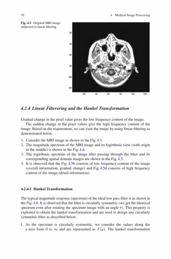
76 4 Medical Image Processing
Fig. 4.3 Original MRI imagesubjected to linear filtering
4.2.4 Linear Filterering and the Hankel Transformation
Gradual change in the pixel value gives the low frequency content of the image.The sudden change in the pixel values give the high frequency content of the
image. Based on the requirement, we can view the image by using linear filtering asdemonstrated below.
1. Consider the MRI image as shown in the Fig. 4.3.2. The magnitude spectrum of the MRI image and its logirthmic view (with origin
in the middle) is shown in the Fig. 4.4.3. The logirthmic spectrum of the image after passing through the filter and its
corresponding spatial domain images are shown in the Fig. 4.5.4. It is observed that the Fig. 4.5b consists of low frequency content of the image
(overall information, gradual change) and Fig. 4.5d consists of high frequencycontent of the image (detail information).
4.2.4.1 Hankel Transformation
The typical magnitude response (spectrum) of the ideal low pass filter is as shown inthe Fig. 4.6. It is observed that the filter is circularly symmetric (we get the identicalspectrum even after rotating the spectrum image with an angle θ ). This property isexploited to obtain the hankel transformation and are used to design any circularlysymmetric filter as described below.
1. As the spectrum is circularly symmetric, we consider the values along they-axis from 0 to ∞ and are represented as F(q). The hankel transformation

4.2 Image Enhancement 77
Fig. 4.4 Original spectrum and the logirthmic spectrum of the MRI image (with origin) in themiddle
(refer Appendix) of the function F(q) is given as
f (r) = 2π
∞∫
0
q F(q)J0(2πqr) (4.1)
where,
J0(q) = 1
π
π∫
0
cos(qsin(φ)) (4.2)
2. Thus the hankel transformation is applied to the function F(q) to obtain f (r).3. The values of F(r) are treated as the polar representation of the spatial domain
F(r, θ) for all the angle θ .4. For the 2D-filter specification shown in the Fig. 4.6, the spatial domain of filter
obtained using the direct method (2D-IDFT) and the hankel transformation are

78 4 Medical Image Processing
Fig. 4.5 a Logirthmic low pass spectrum. b Image corresponding to low pass spectrum. c Logirth-mic high pass spectrum. d Image corresponding to high pass spectrum
shown in the figure. It is noted that the spatial domain obtaining using the hankeltransformation requires lesser number of computation to obtain the spatial domain.
5. Note that in case of continous hankel transformation, the 2D-filter specificationis perfectly circular symmetric and hence 2D-FFT consists of only the real com-ponents.
6. Ideally (1) and (4) subplots of the Fig. 4.6 must be identical. The variation is dueto the imperfection in the circular symmetry while realizing in discrete form.
4.2.4.2 hankeltransformation.m
%Demonstration of Hankel transformationA=zeros(31,31);a=ones(1,15);for r=0:1:9for theta=0:(2*pi)/360:(2*pi);x=round(r*cos(theta));y=round(r*sin(theta));
A(x+16,y+16)=a(r+1);

4.2 Image Enhancement 79
Fig. 4.6 a Circular symmetric filter with origin as the center. b Corresponding spatial domain(magnitude) obtained using 2D-IDFT. c Spatial domain (magnitude) obtained using Hankel trans-formation. d Magnitude of 2D-FFT of spatial domain obtained using Hankel transformation
endendB=ifft2(A);B=fftshift(B);%The above 2D-IDFT is realized using Hankel transformation%as described%below.F=[];for i=16:1:31
F=[F A(i,16)];ends=0;for q=0:1:15for r=1:1:14
s=s+2*pi*2*r*F(r+1)*Jbessel(2*pi*q*r/31);ends=s+F(16)*Jbessel(2*pi*q*15/31)f(q+1)=s;s=0;end
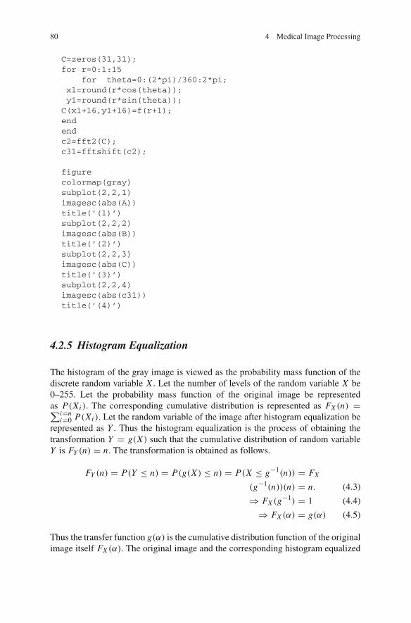
80 4 Medical Image Processing
C=zeros(31,31);for r=0:1:15
for theta=0:(2*pi)/360:2*pi;x1=round(r*cos(theta));y1=round(r*sin(theta));
C(x1+16,y1+16)=f(r+1);endendc2=fft2(C);c31=fftshift(c2);
figurecolormap(gray)subplot(2,2,1)imagesc(abs(A))title(’(1)’)subplot(2,2,2)imagesc(abs(B))title(’(2)’)subplot(2,2,3)imagesc(abs(C))title(’(3)’)subplot(2,2,4)imagesc(abs(c31))title(’(4)’)
4.2.5 Histogram Equalization
The histogram of the gray image is viewed as the probability mass function of thediscrete random variable X . Let the number of levels of the random variable X be0–255. Let the probability mass function of the original image be representedas P(Xi ). The corresponding cumulative distribution is represented as FX (n) =∑i=n
i=0 P(Xi ). Let the random variable of the image after histogram equalization berepresented as Y . Thus the histogram equalization is the process of obtaining thetransformation Y = g(X) such that the cumulative distribution of random variableY is FY (n) = n. The transformation is obtained as follows.
FY (n) = P(Y ≤ n) = P(g(X) ≤ n) = P(X ≤ g−1(n)) = FX
(g−1(n))(n) = n. (4.3)
⇒ FX (g−1) = 1 (4.4)
⇒ FX (α) = g(α) (4.5)
Thus the transfer function g(α) is the cumulative distribution function of the originalimage itself FX (α). The original image and the corresponding histogram equalized
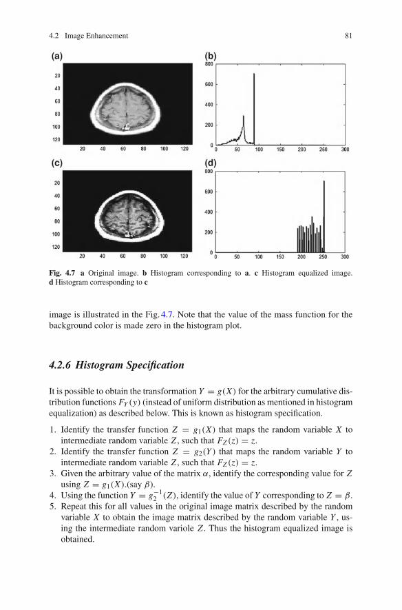
4.2 Image Enhancement 81
Fig. 4.7 a Original image. b Histogram corresponding to a. c Histogram equalized image.d Histogram corresponding to c
image is illustrated in the Fig. 4.7. Note that the value of the mass function for thebackground color is made zero in the histogram plot.
4.2.6 Histogram Specification
It is possible to obtain the transformation Y = g(X) for the arbitrary cumulative dis-tribution functions FY (y) (instead of uniform distribution as mentioned in histogramequalization) as described below. This is known as histogram specification.
1. Identify the transfer function Z = g1(X) that maps the random variable X tointermediate random variable Z , such that FZ (z) = z.
2. Identify the transfer function Z = g2(Y ) that maps the random variable Y tointermediate random variable Z , such that FZ (z) = z.
3. Given the arbitrary value of the matrix α, identify the corresponding value for Zusing Z = g1(X).(say β).
4. Using the function Y = g−12 (Z), identify the value of Y corresponding to Z = β.
5. Repeat this for all values in the original image matrix described by the randomvariable X to obtain the image matrix described by the random variable Y , us-ing the intermediate random variole Z . Thus the histogram equalized image isobtained.

82 4 Medical Image Processing
4.2.6.1 histogramequalization.m
%Histogram equalizationload mriA=D(:,:,:,25);A=A(1:1:127,1:1:127);B=histeq(A)’;figurecolormap(gray)subplot(2,2,1)imagesc(A)subplot(2,2,2)plot(imhist(A))a=imhist(A);a(1)=0;plot(a)subplot(2,2,3)B=imrotate(B,-90);imagesc(B)subplot(2,2,4)b=imhist(B)b(187)=0;plot(b)
4.3 Image Compression
4.3.1 Discrete Cosine Transformation (DCT)
The following steps are followed to compress the image using DCT.
1. Subtract 128 from all the pixel values to obtain the DC component 0.2. Divide the image into subblock of size 8×8.3. Each subblock is subjected to 2D-DCT.4. Divide each sub-block with the quantization mask (JPEG Mask) and round it. We
get more number of zeros. The quantized data from each sublock is collected inthe zig-zag fashion and are stored using run-length and Huffmann coding.
5. Hence image is compressed using 2D-DCT. Refer Fig. 4.8 to view the originaland the corresponding compressed image obtained using 2D-DCT ( Figs. 4.9and 4.10).
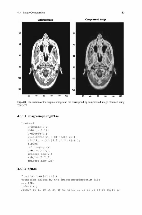
4.3 Image Compression 83
Fig. 4.8 Illustration of the original image and the corresponding compressed image obtained using2D-DCT
4.3.1.1 imagecompusingdct.m
load mriD=double(D);V=D(:,:,1,1);V=double(V);V1=blkproc(V,[8 8],’dctt(x)’);V2=blkproc(V1,[8 8],’idctt(x)’);figurecolormap(gray)subplot(1,2,1)imagesc(abs(V))subplot(1,2,2)imagesc(abs(V2))
4.3.1.2 dctt.m
function [res]=dctt(x)%Function called by the imagecompusingdct.m filex=x-128;x=dct2(x);JPEGQ=[16 11 10 16 24 40 51 61;12 12 14 19 26 58 60 55;14 13

84 4 Medical Image Processing
Fig. 4.9 a Original image. b 1:5.12 Compressed image using KL-Transformation. c 1:2.56 Com-pressed image using KL-Transformation
16 24 40 57 69 56;...14 17 22 29 51 87 80 62;18 22 37 56 68 109 103 77;24 3555 64 81 104 113 92;...49 64 78 87 103 121 120 101;72 92 95 98 112 100 103 99];
res=round(x./JPEGQ);
4.3.1.3 idctt.m
function [res]=idctt(x)%Function called by the imagecompusingdct.m fileJPEGQ=[16 11 10 16 24 40 51 61;12 12 14 19 26 58 60 55;14 13
16 24 40 57 69 56;...14 17 22 29 51 87 80 62;18 22 37 56 68 109 103 77;24 35 5564 81 104 113 92;...49 64 78 87 103 121 120 101;72 92 95 98 112 100 103 99];
x=x.*JPEGQ;x=idct2(x);res=x+128;

4.3 Image Compression 85
Fig. 4.10 Original image and the first level wavelet decomposed images using db6 filter
4.3.2 Using KL-Transformation
1. Consider the group of similar medical images to be compressed. Example: MRIimages.
2. Every column of the individual medical image is treated as the vector.3. Compute the co-variance matrix C using the collected vectors.4. Compute the significant eigen vectors of the C corresponding to the significant
eigen values.5. Represent each column of the image to be compressed as the linear combinations
of significant vectors. The corresponding co-efficients are stored along with thesignificant eigen vectors as the compressed data.
6. Significant eigen vectors are common for all the images. The corresponding co-efficients along with the stored significant eigen vectors are used to reconstructthe image back.
7. Number of significant eigen vectors determines the quality of the reconstructedimage.
8. 27 MRI images each with size 128 × 128 is considered to demonstrate the KLTbased compression.
9. Every image is reconstructed back with two different compression ratio and aredisplayed in the Fig. 2.3. One with 50 significant eigen vectors ( compression ratio1:2.56) and another with 25 significant eigen vectors (compression ratio 1:5.12).

86 4 Medical Image Processing
4.3.2.1 kltformedimagecomp.m
%Medical image compression using KL-Transformation%Each column of the image is treated as the vector.
load mriD=double(D);%collecting the vectorsvect=[];for i=1:1:27
vect=[vect D(:,:,1,i)];endvect=double(vect);%Computing the inner-product matrixvect=double(vect);C=cov(double(vect’));[E,V]=eigs(C,50);%Compression starts here%The co-efficients to be stored (to store all the images ) is as follows.%Compression for the first image
a=[25 50];p=1;for i=1:5:27I=double(D(:,:,i));subplot(6,3,p)p=p+1colormap(gray)imagesc(I)for cr=1:1:2COEF=[ ];
E1=E(:,1:1:a(cr));for j=1:1:128COEF=[COEF E1’*I(:,j)];end%Reconstructionfor k=1:1:128
R(:,k)=E1*COEF(:,k);endsubplot(6,3 ,p)colormap(gray)imagesc(R)p=p+1endend
4.4 Feature Extraction and Classification
To help the automated system to classify the medical images into normal and ab-normal categories, the features are extracted from the medical image to train theclassifier. The feature vector extracted using the wavelet transformation is describedbelow.

4.4 Feature Extraction and Classification 87
Table 4.1 Discrete WaveletTransformation (DWT)
Row-wise Column-wise Type1
Low pass Low pass ApproximationLow pass High pass HorizontalHigh pass Low pass VerticalHigh pass High pass Diagonal
4.4.1 Using Discrete Wavelet Transformation
1. Discrete wavelet transformation (DWT) consists of four discrete 1D-filters. Theyare low pass decomposition filter, high pass decomposition, corresponding lowpass reconstruction filter and high pass reconstruction filter.
2. Every row of the medical image under consideration is passed through the 1D-filter 1.
3. Every column of the obtained image is passed through the 1D-filter 2.4. The alternative samples are removed from the obtained image to obtain the
Wavelet decomposed image.5. Based on the combinations of the filter-1 and filter-2 selected from the low-pass
and the high-pass decomposition filters, we obtain approximation, horizontal,vertical and the diagonal images of first level decomposition (refer Table 4.1).
6. The approximation of the first level decomposed image is treated as the originalimage and are subjected to decomposition to obtain second level decomposition(refer Fig. 4.11) and so on.
7. The decomposed values (significant) of last level approximation image and all thehorizontal, vertical and diagonal values (upto to the last level decomposition) arecollected as the vector and are treated as feature vector for further classification.
8. Based on the type of 1D filters used, we obtain different wavelet decomposition.The db6 1D-filters are used for illustration.
9. Corresponding recomposition filters are used for DWT based medical image com-pression and denoising. Decomposition filters are not used for feature extraction.
4.4.1.1 feaextwavelet.m
load mriA=D(:,:,1,14);[C,L]=wavedec2(A,2,’db6’);A=appcoef2(C,L,’db6’,2);[H2,V2,D2]=detcoef2(’all’,C,L,2);[H1,V1,D1]=detcoef2(’all’,C,L,1);
figurecolormap(gray)

88 4 Medical Image Processing
Fig. 4.11 Second level wavelet decomposed images using db6 filter
subplot(2,2,1)imagesc(A)subplot(2,2,2)imagesc(H2)subplot(2,2,3)imagesc(V2)subplot(2,2,4)imagesc(D2)figurecolormap(gray)subplot(2,2,1)imagesc(D(:,:,1,14))subplot(2,2,2)imagesc(H1)subplot(2,2,3)imagesc(V1)subplot(2,2,4)imagesc(D1)

4.4 Feature Extraction and Classification 89
4.4.2 Dimensionality Reduction Using PrincipalComponent Analysis (PCA)
The features that highlights the discrimination between the different groups arecollected from the individual images and are collected as the feature vectors. Thedimension of such collected vectors are usually large. There is the need to map thosevectors to the lower dimensional space for further classification. This is achieved byidentifying the transformation matrix W T of size m × n that maps the vector v ofsize n × 1 to the vector u of size m × 1, where m � n. One way to achieve the sameis to use the KL-Transformation (refer Sect. 4.3.2) and are known as Principal Com-ponent Analysis (PCA). The steps involved in dimensionality reduction using PCA,followed by the simple euclidean distance based classifier is summarized below.
1. Consider the first 24 frames of the MRI image are grouped (refer Fig. 4.12) intofour categories (based on the time it occur).
2. First three columns of the images in the Fig. 4.12 are treated as the training set.The remaining data are treated as the testing images.
3. For simplicity the actual image is resized to the size of 12×12 and are reshapedto 1 × 144 to obtain the feature vector. (Note that in practice, suitable featureextraction is applied).
4. Apply KL-Transformation (refer Sect. 4.3.2) to obtain the significant eigen vec-tors.
5. The dimension of the projected vector depends on the selection of the numberof significant eigen vectors.
6. For instance, if one eigen vector is selected, the dimension of the projected vectoris 1 × 1. If two significant vectors are selected, the dimension of the projectedvector is 2 × 1. The projection using the PCA basis maximizes the variances ofthe individual elements of the projected vectors (refer Appendix B).
7. The projected 1D and 2D vectors corresponding to the training set is displayedin the Figs. 4.13 and 4.14 respectively.
8. The mean of the projected vectors corresponding to the individual groups arecomputed and are stored for further classification of unknown vectors.
9. For the arbitrary test image(I), feature vector is collected and are projected tothe lower dimensional space using the corresponding transformation matrix. Theeuclidean distance of the projected vector with the mean vectors of the individualgroups of the projected vectors are computed. Identify the group that belongs tothe lowest euclidean distance (say group G) and declare that the arbitrary testimage (I) belongs to the group G.
10. The classification procedure (based on eculidean distance) is repeated for allthe test images and the corresponding declared group number is displayed inTable 4.3 along with the corresponding original group number. The percentageof correct classification are given as 66.67 and 50 respectively with the 1D and2D projection.
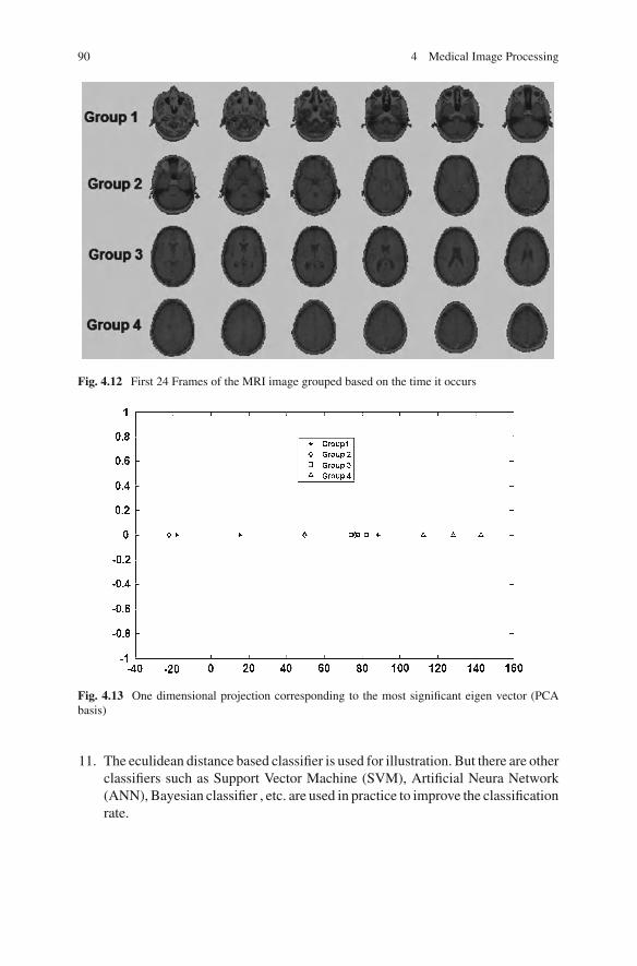
90 4 Medical Image Processing
Fig. 4.12 First 24 Frames of the MRI image grouped based on the time it occurs
Fig. 4.13 One dimensional projection corresponding to the most significant eigen vector (PCAbasis)
11. The eculidean distance based classifier is used for illustration. But there are otherclassifiers such as Support Vector Machine (SVM), Artificial Neura Network(ANN), Bayesian classifier , etc. are used in practice to improve the classificationrate.

4.4 Feature Extraction and Classification 91
Fig. 4.14 Two dimensional projection with two eigen vectors corresponding to the largest twoeigen values (PCA basis)
4.4.2.1 projection1d-2d-pca.m
%PCA based Dimensionality reduction
load mrifigurecolormap(map)montage(D)tr=[1 3 5 7 9 11 13 15 17 19 21 23];COLLECT=[ ];D=double(D);for i=1:1:12
D1=imresize(D(:,:,1,tr(i)),[12 12]);COLLECT=[COLLECT; reshape(D1,1,12*12)];
endC=cov(COLLECT,1);
%1D projection for the training data[EV1,DV1]=eigs(C,1);ONEDPV=EV1’*COLLECT’figureplot(ONEDPV(1:3),zeros(1,3),’*’)hold onplot(ONEDPV(4:6),zeros(1,3),’d’)hold onplot(ONEDPV(7:9),zeros(1,3),’s’)hold on
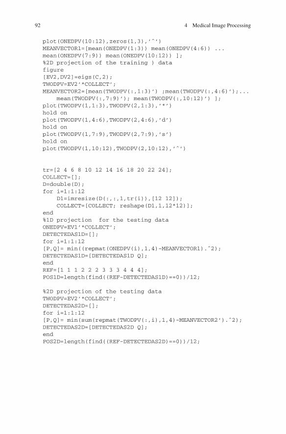
92 4 Medical Image Processing
plot(ONEDPV(10:12),zeros(1,3),’ˆ’)MEANVECTOR1=[mean(ONEDPV(1:3)) mean(ONEDPV(4:6)) ...mean(ONEDPV(7:9)) mean(ONEDPV(10:12)) ];%2D projection of the training ) datafigure[EV2,DV2]=eigs(C,2);TWODPV=EV2’*COLLECT’;MEANVECTOR2=[mean(TWODPV(:,1:3)’) ;mean(TWODPV(:,4:6)’);...
mean(TWODPV(:,7:9)’); mean(TWODPV(:,10:12)’) ];plot(TWODPV(1,1:3),TWODPV(2,1:3),’*’)hold onplot(TWODPV(1,4:6),TWODPV(2,4:6),’d’)hold onplot(TWODPV(1,7:9),TWODPV(2,7:9),’s’)hold onplot(TWODPV(1,10:12),TWODPV(2,10:12),’ˆ’)
tr=[2 4 6 8 10 12 14 16 18 20 22 24];COLLECT=[];D=double(D);for i=1:1:12
D1=imresize(D(:,:,1,tr(i)),[12 12]);COLLECT=[COLLECT; reshape(D1,1,12*12)];
end%1D projection for the testing dataONEDPV=EV1’*COLLECT’;DETECTEDAS1D=[];for i=1:1:12[P,Q]= min((repmat(ONEDPV(i),1,4)-MEANVECTOR1).ˆ2);DETECTEDAS1D=[DETECTEDAS1D Q];endREF=[1 1 1 2 2 2 3 3 3 4 4 4];POS1D=length(find((REF-DETECTEDAS1D)==0))/12;
%2D projection of the testing dataTWODPV=EV2’*COLLECT’;DETECTEDAS2D=[];for i=1:1:12[P,Q]= min(sum(repmat(TWODPV(:,i),1,4)-MEANVECTOR2’).ˆ2);DETECTEDAS2D=[DETECTEDAS2D Q];endPOS2D=length(find((REF-DETECTEDAS2D)==0))/12;
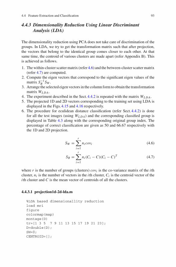
4.4 Feature Extraction and Classification 93
4.4.3 Dimensionality Reduction Using Linear DiscriminantAnalysis (LDA)
The dimensionality reduction using PCA does not take care of discrimination of thegroups. In LDA, we try to get the transformation matrix such that after projection,the vectors that belong to the identical group comes closer to each other. At thatsame time, the centroid of various clusters are made apart (refer Appendix B). Thisis achieved as follows.
1. The within-cluster scatter matrix (refer 4.6) and the between-cluster scatter matrix(refer 4.7) are computed.
2. Compute the eigen vectors that correspond to the significant eigen values of thematrix S−1
B SW .3. Arrange the selected eigen vectors in the column form to obtain the transformation
matrix WL D A.4. The experiment described in the Sect. 4.4.2 is repeated with the matrix WL D A.5. The projected 1D and 2D vectors corresponding to the training set using LDA is
displayed in the Figs. 4.15 and 4.16 respectively.6. The procedure for eculidean distance classification (refer Sect. 4.4.2) is done
for all the test images (using WL D A) and the corresponding classified group isdisplayed in Table 4.3 along with the corresponding original group index. Thepercentage of correct classification are given as 50 and 66.67 respectively withthe 1D and 2D projection.
SW =r∑
i=1
ni covi (4.6)
SB =r∑
i=1
ni (Ci − C)(Ci − C)T (4.7)
where r is the number of groups (clusters) covi is the co-variance matrix of the i thcluster, ni is the number of vectors in the i th cluster, Ci is the centroid vector of thei th cluster and C is the mean vector of centroids of all the clusters.
4.4.3.1 projection1d-2d-lda.m
%LDA based dimensionallity reductionload mrifigurecolormap(map)montage(D)tr=[1 3 5 7 9 11 13 15 17 19 21 23];D=double(D);SW=0;CENTROID=[];

94 4 Medical Image Processing
Fig. 4.15 One dimensional projection corresponding to the most significant eigen vector (LDAbasis)
Fig. 4.16 Two dimensional projection with two eigen vectors corresponding to the largest twoeigen values (LDA basis)
for j=1:1:4COLLECT=[];for i=1:1:3
D1=imresize(D(:,:,1,tr(3*(j-1)+i)),[12 12]);COLLECT=[COLLECT; reshape(D1,1,12*12)];
endCENTROID=[CENTROID;mean(COLLECT)];

4.4 Feature Extraction and Classification 95
SW=SW+cov(COLLECT);endSB=cov(CENTROID);
COLLECT=[ ];for i=1:1:12
D1=imresize(D(:,:,1,tr(i)),[12 12]);COLLECT=[COLLECT; reshape(D1,1,12*12)];
end%1D projection for the training data[E1,V1]=eigs(pinv(SB)*SW,1);ONEDPV=E1’*COLLECT’figureplot(ONEDPV(1:3),zeros(1,3),’*’)hold onplot(ONEDPV(4:6),zeros(1,3),’d’)hold onplot(ONEDPV(7:9),zeros(1,3),’s’)hold onplot(ONEDPV(10:12),zeros(1,3),’ˆ’)MEANVECTOR1=[mean(ONEDPV(1:3)) mean(ONEDPV(4:6))...mean(ONEDPV(7:9)) mean(ONEDPV(10:12)) ];
%2D projection of the training datafigure[E2,V2]=eigs(pinv(SB)*SW,2);TWODPV=E2’*COLLECT’;MEANVECTOR2=[mean(TWODPV(:,1:3)’) ;mean(TWODPV(:,4:6)’);...
mean(TWODPV(:,7:9)’); mean(TWODPV(:,10:12)’) ];plot(TWODPV(1,1:3),TWODPV(2,1:3),’*’)hold onplot(TWODPV(1,4:6),TWODPV(2,4:6),’d’)hold onplot(TWODPV(1,7:9),TWODPV(2,7:9),’s’)hold onplot(TWODPV(1,10:12),TWODPV(2,10:12),’ˆ’)
tr=[2 4 6 8 10 12 14 16 18 20 22 24];COLLECT=[];D=double(D);for i=1:1:12
D1=imresize(D(:,:,1,tr(i)),[12 12]);COLLECT=[COLLECT; reshape(D1,1,12*12)];
end
%1D projection for the testing dataONEDPV=E1’*COLLECT’;DETECTEDAS1D=[];for i=1:1:12

96 4 Medical Image Processing
[P,Q]= min((repmat(ONEDPV(i),1,4)-MEANVECTOR1).ˆ2);DETECTEDAS1D=[DETECTEDAS1D Q];endREF=[1 1 1 2 2 2 3 3 3 4 4 4];POS1D=length(find((REF-DETECTEDAS1D)==0))/12;
%2D projection of the testing dataTWODPV=E2’*COLLECT’;DETECTEDAS2D=[];for i=1:1:12[P,Q]= min(sum(repmat(TWODPV(:,i),1,4)-MEANVECTOR2’).ˆ2);DETECTEDAS2D=[DETECTEDAS2D Q];endPOS2D=length(find((REF-DETECTEDAS2D)==0))/12;
4.4.4 Dimensionality Reduction Using Kernel-LinearDiscriminant Analysis (K-LDA)
Although discrimination is taken care in LDA, the clusters in the projected space areoverlapping in nature. Intuitively, we understand that when the vectors are mapped tothe higher dimensional space, there is the chance to have more separation between theclusters. The LDA formulated using the mapped vectors in the higher dimensionalspace involves the inner-product of the mapped vectors rather than the mapped vectoritself. (i.e) Let the vector u and v are present in the lower dimensional space. Also letthe corresponding transformed vectors in the higher dimensional space be representedas φ(u) and φ(v) respectively. The LDA formulated using the projected vectorsdoesn’t involve φ(u) and φ(v) explicitly (refer Appendix B), instead it involvesφ(u)T φ(v) (the inner-product values of the projected vectors). Hence if we are ableto find the function k (kernel function) such that k(u, v) = φ(u)T φ(v), there is noneed of explicit mapping to the higher dimensional space. This lead to the techniquecalled Kernel-Linear discriminant analysis as described below.
1. Arrange all the training vectors in the column form to obtain the matrix M .2. Compute the kernel matrix K = k(MT M),where k is the kernel function. The
list of mostly used kernel function is listed in the Table 4.2.3. The columns of the matrix K are considered as the training vectors in the inner-
product space.4. Compute the LDA basis (refer Sect. 4.4.3) in the inner-product space. Arrange
them in the columnwise to obtain the transformation matrix WK to map to thelower dimensional space.
5. Any arbitrary vector v in the feature space is mapped to the kernel space us-ing k(MT v). This is further mapped to the lower dimensional space using thetransformation matrix WK as WK k(MT v).

4.4 Feature Extraction and Classification 97
Table 4.2 List of mostly used kernel functions
Name Kernel function k(x1, x2)
Innerproduct kernel (x1T x2)
Gaussian exp−||x1−x2||2
c1
Polynomial (x1T x2 + c2)c3
Table 4.3 Classification using PCA,LDA and K-LDA projection
ORIGINAL GROUP 1 1 1 2 2 2 3 3 3 4 4 4Classified using 1D PCA 3 1 1 1 3 3 3 3 3 4 4 4Classified using 2D PCA 4 3 2 2 3 3 3 3 1 4 4 4Classified using 1D LDA 3 2 2 2 1 4 3 3 3 4 4 1Classified using 2D LDA 4 1 2 2 2 3 3 3 1 4 4 4Classified using 1D K-LDAa 3 2 2 2 3 3 3 3 3 3 4 2Classified using 2D K-LDAa 1 1 2 2 3 2 3 3 1 4 4 4a Using gaussian kernel
Fig. 4.17 One dimensionalprojection corresponding tothe most significant eigenvector (K-LDA basis)
6. The experiment described in the Sect. 4.4.2 is repeated with the transformationmatrix WK and the transformation WK k(MT v).
7. The projected 1D and 2D vectors corresponding to the training set using K-LDAis displayed in the Figs. 4.17 and 4.18 respectively.
8. The procedure for eculidean distance classification (refer Sect. 4.4.2) is done forall the testing images (using the transformation matrix WK and the transformationWK k(MT v)) and the corresponding classified group is displayed in Table 4.3along with the corresponding original group index. The percentage of correctclassification are given as 41.67 and 75 respectively with the 1D and 2D projection.
4.4.4.1 projection1d-2d-klda.m
%KLDA based dimensionallity reductionload mri

98 4 Medical Image Processing
Fig. 4.18 Two dimensionalprojection with two eigenvectors corresponding tothe largest two eigen values(K-LDA basis)
figurecolormap(map)montage(D)tr=[1 3 5 7 9 11 13 15 17 19 21 23];D=double(D);COLLECT1=[ ];for i=1:1:12
D1=imresize(D(:,:,1,tr(i)),[12 12]);COLLECT1=[COLLECT1; reshape(D1,1,12*12)];
endCOLLECT1=COLLECT1’;%Computing the kernel matrixK=[];for i=1:1:12
for j=1:1:12K(j,i)=k11(COLLECT1(:,i),COLLECT1(:,j),1)
endend
SW=0;CENTROID=[];for j=1:1:4COLLECT=K(:,(3*(j-1)+1):1:(3*(j-1)+3));CENTROID=[CENTROID;mean(COLLECT’)];SW=SW+cov(COLLECT’);endSB=cov(CENTROID);
%1D projection for the training data[E1,V1]=eigs(pinv(SB)*SW,1);ONEDPV=E1’*K’;figureplot(ONEDPV(1:3),zeros(1,3),’*’)
4.4 Feature Extraction and Classification 99
hold onplot(ONEDPV(4:6),zeros(1,3),’d’)hold onplot(ONEDPV(7:9),zeros(1,3),’s’)hold onplot(ONEDPV(10:12),zeros(1,3),’ˆ’)MEANVECTOR1=[mean(ONEDPV(1:3)) mean(ONEDPV(4:6)) ...mean(ONEDPV(7:9)) mean(ONEDPV(10:12)) ];%2D projection of the training datafigure[E2,V2]=eigs(pinv(SB)*SW,2);TWODPV=E2’*K’;MEANVECTOR2=[mean(TWODPV(:,1:3)’) ;mean(TWODPV(:,4:6)’);...
mean(TWODPV(:,7:9)’); mean(TWODPV(:,10:12)’) ];plot(TWODPV(1,1:3),TWODPV(2,1:3),’*’)hold onplot(TWODPV(1,4:6),TWODPV(2,4:6),’d’)hold onplot(TWODPV(1,7:9),TWODPV(2,7:9),’s’)hold onplot(TWODPV(1,10:12),TWODPV(2,10:12),’ˆ’)
tr=[2 4 6 8 10 12 14 16 18 20 22 24];D=double(D);COLLECT2=[ ];for i=1:1:12
D1=imresize(D(:,:,1,tr(i)),[12 12]);COLLECT2=[COLLECT2; reshape(D1,1,12*12)];
endCOLLECT2=COLLECT2’;Ktest=[];for i=1:1:12
for j=1:1:12Ktest(j,i)=k11(COLLECT2(:,i),COLLECT1(:,j),1);
endend
%1D projection for the testing dataONEDPV=E1’*Ktest;DETECTEDAS1D=[];for i=1:1:12[P,Q]= min((repmat(ONEDPV(i),1,4)-MEANVECTOR1).ˆ2);DETECTEDAS1D=[DETECTEDAS1D Q];endREF=[1 1 1 2 2 2 3 3 3 4 4 4];POS1D=length(find((REF-DETECTEDAS1D)==0))/12;
%2D projection of the testing data

100 4 Medical Image Processing
TWODPV=E2’*Ktest;DETECTEDAS2D=[];for i=1:1:12[P,Q]= min(sum(repmat(TWODPV(:,i),1,4)-MEANVECTOR2’).ˆ2);DETECTEDAS2D=[DETECTEDAS2D Q];endPOS2D=length(find((REF-DETECTEDAS2D)==0))/12;
In general the percentage of classification depends on the following.
1. Type of the feature vector.2. Type of the projection technique.3. Dimension of the projected vectors.4. Number of training data.5. Type of the classifier.

Appendix ASolving Bloch Equation with ADvsincðDvtÞEnvelope
Rewriting (2.21) and (2.23) with ADvsincðDvtÞ envelope as follows with thecondition Dv\\ B0c
2p .
dMxyðtÞdt
¼ jcADvsincðDvtÞM0cosðaÞejð�cB0tþhÞ ðA:1Þ
dMzðtÞdt
¼ cADvsincðDvtÞM0sinðaÞE0sinðh� /Þ ðA:2Þ
Since sincðDvtÞ is almost one for all t with Dv\\ B0c2p , we treat sincðDvtÞ as the
constant in both the equations and solution is obtained as follows
MxyðtÞ ¼ 2M0sinðaÞejð�cB0tþ/Þ ðA:3Þ
MzðtÞ ¼ cM0sinðaÞADvsincðDvtÞsinðh� /Þt þ 2M0cosðaÞ ðA:4Þ
E. S. Gopi, Digital Signal Processing for Medical Imaging Using Matlab,DOI: 10.1007/978-1-4614-3140-4, � Springer Science+Business Media New York 2013
101

Appendix BProjection Techniques
When the number of samples in the feature vector is large, the computationalcomplexity in computing the decision boundary between the different clustersincreases. Therefore, there is a requirement to map the feature vector into thelower dimensional space; thereby reducing the computational complexity. Thismapping is achieved by using transformation matrix WT obtained as describedbelow.
B.1 Principal Component Analysis
The covariance matrix of the vectors in the vector space is given asCX ¼ EððX � lXÞðX � lXÞTÞ, where X is the random vector asssociated with thevectors in the vector space (V), lX is the mean vector of the vector space.Thediagonal elements of the matrix CX gives the variance of the individual elements ofthe random variable X. Let the size of the random vector X be m� 1 and thetransformation vector W1 of size m� 1 is used to transform the random vector X torandom variable Y1 as Y1 ¼ WT
1 X. Note that the random variable Y1 is of the size1� 1. Let us formulate the objective function to optimize the vector W1 such thatthe variance of the random variable Y1 is maximized, subject to the constraint thatWT
1 W1 ¼ 1. Note the variance of the random variable Y is given as CY ¼ WT1 CXW1.
The solution is obtained as follows. The lagrangean equation is given as
J ¼ WT1 CXW1 þ kðWT
1 W1 � 1Þ ðB:1Þ
differentiating with respect to the W1 and equate to zero and solve for W1
(exploiting the property of the symmetry of the covariance matrix CX), we getCXW1 ¼ �kW1. This indicate that the W1 is the eigen vector corresponding to theeigen value �k. To maximize the function, we have to choose the eigen vectorcorresponding to the largest eigen value.
Thus in general the eigen vectors of the co-variance matrix CX corresponding thelargest n significant eigen values are arranged in columnwise to obtain the
E. S. Gopi, Digital Signal Processing for Medical Imaging Using Matlab,DOI: 10.1007/978-1-4614-3140-4, � Springer Science+Business Media New York 2013
103
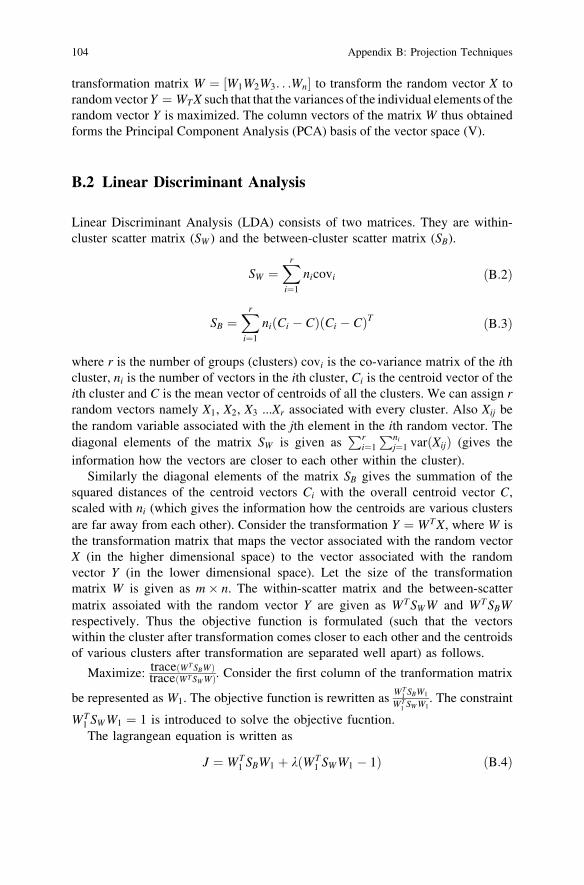
transformation matrix W ¼ ½W1W2W3. . .Wn� to transform the random vector X torandom vector Y ¼ WT X such that that the variances of the individual elements of therandom vector Y is maximized. The column vectors of the matrix W thus obtainedforms the Principal Component Analysis (PCA) basis of the vector space (V).
B.2 Linear Discriminant Analysis
Linear Discriminant Analysis (LDA) consists of two matrices. They are within-cluster scatter matrix (SW ) and the between-cluster scatter matrix (SB).
SW ¼Xr
i¼1
nicovi ðB:2Þ
SB ¼Xr
i¼1
niðCi � CÞðCi � CÞT ðB:3Þ
where r is the number of groups (clusters) covi is the co-variance matrix of the ithcluster, ni is the number of vectors in the ith cluster, Ci is the centroid vector of theith cluster and C is the mean vector of centroids of all the clusters. We can assign rrandom vectors namely X1, X2, X3 ...Xr associated with every cluster. Also Xij bethe random variable associated with the jth element in the ith random vector. Thediagonal elements of the matrix SW is given as
Pri¼1
Pnij¼1 varðXijÞ (gives the
information how the vectors are closer to each other within the cluster).Similarly the diagonal elements of the matrix SB gives the summation of the
squared distances of the centroid vectors Ci with the overall centroid vector C,scaled with ni (which gives the information how the centroids are various clustersare far away from each other). Consider the transformation Y ¼ WT X, where W isthe transformation matrix that maps the vector associated with the random vectorX (in the higher dimensional space) to the vector associated with the randomvector Y (in the lower dimensional space). Let the size of the transformationmatrix W is given as m� n. The within-scatter matrix and the between-scattermatrix assoiated with the random vector Y are given as WT SWW and WT SBWrespectively. Thus the objective function is formulated (such that the vectorswithin the cluster after transformation comes closer to each other and the centroidsof various clusters after transformation are separated well apart) as follows.
Maximize: traceðWT SBWÞtraceðWT SW WÞ. Consider the first column of the tranformation matrix
be represented as W1. The objective function is rewritten asWT
1 SBW1
WT1 SW W1
. The constraint
WT1 SW W1 ¼ 1 is introduced to solve the objective fucntion.The lagrangean equation is written as
J ¼ WT1 SBW1 þ kðWT
1 SW W1 � 1Þ ðB:4Þ
104 Appendix B: Projection Techniques

differentiating the equation with respect to W1 (exploiting the property of symmetryproperty of the matrices SB and SW and equate to zero gives the solution as the eigenvector corresponding to the matrix S�1
W SB corresponding to the largest eigen value.The other columns of the matrix W are the eigen vectors corresponding to the nextlargest eigen values.Thus the eigen vectors corresponding to the significant eigenvalues of the matrix S�1
W SB are arranged column wise to obtain the matrix W . Thecolumn vectors thus obtained form the LDA basis of the vector space V associatedwith random variable X.
B.3 Kernel-Linear Discriminant Analysis
To improve the performance of LDA by creating wide separation between theclusters in the higher dimensional space, Kernel-Linear Discriminant Analysis(K-LDA) is used. In this technique, the vectos corresponding to the featuredimensional space is mapped to the higher dimensional space. By intuition weunderstand that the map to the higher dimensional space introduces betterseparation. Suppose the transformation /ðXÞ transforms the vector in the featuredimensional space to the higher dimensional space. The between-scatter matrix andwithin-scatter matrix computed using the the transformed vectors are represented asS/B and S/W respectively. The columns of the transformation matrix (W/) to mapfrom this higher dimensional space to the lower dimensional space is given as theeigen vector v/ of S/�1
W S/B (i.e) S/Bv/ ¼ kphiS/W v/. The vector v/ lies inthe vector space spanned by all the training vectors (/ðXÞ) that are used to computethe S/W and S/B. Hence we can represent the vector v/ as following.
For some arbitray vector u.
v/ ¼ ½/ðX1Þ/ðX2Þ . . . /ðXNÞ�u ðB:5Þ
) S/B½/ðX1Þ/ðX2Þ . . . /ðXNÞ�u ¼ kphiS/W ½/ðX1Þ/ðX2Þ . . . /ðXNÞ�u ðB:6Þ
Multiplying ½/ðX1Þ/ðX2Þ . . . /ðXNÞ�T on both sides of (B.6) and representing SKB ¼½/ðX1Þ/ðX2Þ . . . /ðXNÞ�T S/B½/ðX1Þ/ðX2Þ . . . /ðXNÞ� and SKW ¼ ½/ðX1Þ/ðX2Þ . . .
/ðXNÞ�T S/W ½/ðX1Þ/ðX2Þ . . . /ðXNÞ�, we get the following.
SKBu ¼ kphiSKWu) ðB:7Þ
It can be easily verified that SKB and SKW are the between-scatter matrix and thewithin-scatter matrix respectively, computed using the corresponding columns of
the Gram-matrix /ðXÞT/ðXÞ, where /ðXÞ ¼ ½/ðX1Þ/ðX2Þ . . . /ðXNÞ�. Let theeigen vectors of the matrix SK�1
W SKB be arranged in the column-wise to obtain thematrix M. Then the transformation matrix that transforms the vector in the higherdimensional space (/ð:Þ) to the lower dimensional space is given as
½/ðX1Þ/ðX2Þ . . . /ðXNÞ�T M. Let the arbitrary vector in the higher dimensional
Appendix B: Projection Techniques 105

space be represented as /ðqÞ corresponding the feature dimensional vector q. Thecorresponding transformed vector in the lower dimensional space is given as
½/ðX1Þ/ðX2Þ . . . /ðXNÞ�T MÞT/ðqÞ ) MT ½/ðX1Þ/ðX2Þ . . . /ðXNÞ�T/ðqÞ ðB:8Þ
½/ðX1Þ/ðX2Þ . . . /ðXNÞ�T/ðqÞ is the vector in the kernel space corresponding tothe vector in the feature space /ðqÞ. Hence to map the vector to the lowerdimensional space, the following steps are followed.
1. For the arbitrary vector q in the feature space, compute the corresponding
vector in the kernel space as qk ¼ ½kðX1; qÞ kðX2; qÞ . . . kðXN ; qÞ�T .2. Thus the transformed vector to the lower dimensional space is given as MT qk.
106 Appendix B: Projection Techniques

Appendix CHankel Transformation
Hankel transformation is applicable for the image that is circular symmetric.Hence assume f ðx; yÞ is circular symmetric. The 2D-Fourier transformation inpolar form is given as follows.
FðU;VÞ ¼Zp
�p
Z1
0
gðr; hÞe�j2prlrdrdh ðC:1Þ
where l ¼ UcosðhÞ þ VsinðhÞ Note that gðr; hÞ is the polar representation of theoriginal image f ðx; yÞ (It is also the inverve fourier tranformation of the radontranformation of FðU;VÞ), where U ¼ lcosðhÞ and V ¼ lsinðhÞ. As f ðx; yÞ iscircular symmetric, the corresponding radon transformation is identical and hencegðr; hÞ is identical for all h. This implies that the radon transformation of FðU;VÞis independent of h. (i.e) FðU;VÞ is circular symmetric and hence it is enough tocompute the values for the co-ordinates on the y-axis. (i.e) U ¼ 0 and V ¼ 0 to1.Particularly for U ¼ 0 and V ¼ q, we get l ¼ q sinðhÞ. Substituting back to theEq. (C.1), we get
GðqÞ ¼Zp
�p
Z1
0
gðrÞe�j2prqsinðhÞr dr dh ðC:2Þ
) GðqÞ ¼Z0
�p
Z1
0
gðrÞe�j2prqsinðhÞr dr dhþZp
0
Z1
0
gðrÞe�j2prqsinðhÞr dr dh ðC:3Þ
) GðqÞ ¼ 2Zp
0
Z1
0
gðrÞcosð2prqsinðhÞÞr dr dh ðC:4Þ
GðqÞ thus obtained is the hankel transformation of gðrÞ:
E. S. Gopi, Digital Signal Processing for Medical Imaging Using Matlab,DOI: 10.1007/978-1-4614-3140-4, � Springer Science+Business Media New York 2013
107

Appendix DList of m-Files
• 1.2.2.1 parallelbeamprojection.m• 1.3.3.1 Fanbeamprojection.m• 2.3.2.1 resmagneticmoment.m• 3.1.1.1 protondensity.m• 3.2.1.1 t2.m• 3.2.1.2 relaxation.m• 3.2.1.3 dephasing.m• 3.2.2.1 spinechodemonstration• 3.3.1.3 spinechopolar.m• 3.4.0.4 t1.m• 4.2.4.2 hankeltransformation.m• 4.2.6.1 histogramequalization.m• 4.3.1.1 imagecompusingdct.m• 4.3.1.2 dctt.m• 4.3.1.3 idctt.m• 4.3.2.1 kltformedimagecomp.m• 4.4.1.1 feaextwavelet.m• 4.4.2.1 projection1d-2d-pca.m• 4.4.2.1 projection1d-2d-lda.m• 4.4.2.1 projection1d-2d-klda.m
E. S. Gopi, Digital Signal Processing for Medical Imaging Using Matlab,DOI: 10.1007/978-1-4614-3140-4, � Springer Science+Business Media New York 2013
109

Index
T1 MRI image, 35T2 MRI, 35a value, 292D-DFT, 422D-Fourier transformation, 3
AApproximation, 87
BBack-projection, 64Between-cluster, 93Bloch equations, 27
CCarteisian scanning, 44Classification, 86Co-variance matrix, 85Compression ratio, 85Computed tomography (CT), 1, 73Cumulative distribution, 80
DDephasing, 49Diagonal, 87Dimensionality reduction, 89Discrete cosine transformation, 82Discrete wavelet transformation, 87Discretization, 50, 54, 69
EEculidean distance, 93Eigen vectors, 85Envelope, 37Euclidean distance, 89
FFan-beam projection, 1Feature extraction, 86Fourier transformation, 36Free induction decay, 35Frequency domain, 41
GGradient echo, 43, 50
HHankel transformation, 76Helical movement, 33High pass decomposition, 87High pass reconstruction filter, 87Histogram equalization, 80Histogram specification, 81Horizontal, 87
IIFFT2, 51Image compression, 82Image enhancement, 74Image substraction, 74Interpolation, 65
E. S. Gopi, Digital Signal Processing for Medical Imaging Using Matlab,DOI: 10.1007/978-1-4614-3140-4, � Springer Science+Business Media New York 2013
111

JJacobian, 3
KK-space, 43Kernel-linear discriminant analysis, 96Kl-transformation, 89
LLarmor frequency, 29Linear discriminant analysis, 93Linear filterering, 76Linear phase delay, 49Logirthmic display, 74Longituidanal, 35Low pass decomposition, 87Low pass filter, 40Low pass reconstruction filter, 87
MMagnetic resonance imaging, 27, 49Medical image processing, 73
NNon-linear filtering, 74Nuclear medicine image, 73
PParallel beam projection, 1Phase component, 37Pixel, 49Polar scanned, 65Polar scanning, 45Principal component analysis, 89Proton-density, 35, 43
RRadon transformation, 1Receiver antenna, 39
Receiver coil, 40Refocussing, 37Relaxation, 38Rephasing, 61Resolution, 65RF, 35
SSelection gradient, 45Sinc, 36Spatial domain, 49Spatial matrix, 61Spin echo, 45Spin–spin, 38Spiral trajectory, 33
TTransformation matrix, 89Transverse component, 32
UUltrasound image, 73
VVertical, 87
WWithin-cluster, 93
XX-ray image, 73
ZZ-component, 33Z-gradient, 37
112 Index