Embed Size (px)
Citation preview
NASA/TM–2016–219173
Diagonally Implicit Runge-KuttaMethods for Ordinary DifferentialEquations. A Review
Christopher A. KennedyPrivate Professional Consultant, Palo Alto, California
Mark H. CarpenterLangley Research Center, Hampton, Virginia
March 2016
https://ntrs.nasa.gov/search.jsp?R=20160005923 2018-06-30T19:55:37+00:00Z
NASA STI Program . . . in Profile
Since its founding, NASA has been dedicatedto the advancement of aeronautics and spacescience. The NASA scientific and technicalinformation (STI) program plays a key partin helping NASA maintain this importantrole.
The NASA STI Program operates under theauspices of the Agency Chief InformationOfficer. It collects, organizes, provides forarchiving, and disseminates NASA’s STI.The NASA STI Program provides access tothe NASA Aeronautics and Space Databaseand its public interface, the NASA TechnicalReport Server, thus providing one of thelargest collection of aeronautical and spacescience STI in the world. Results arepublished in both non-NASA channels andby NASA in the NASA STI Report Series,which includes the following report types:
• TECHNICAL PUBLICATION. Reports ofcompleted research or a major significantphase of research that present the resultsof NASA programs and include extensivedata or theoretical analysis. Includescompilations of significant scientific andtechnical data and information deemed tobe of continuing reference value. NASAcounterpart of peer-reviewed formalprofessional papers, but having lessstringent limitations on manuscript lengthand extent of graphic presentations.
• TECHNICAL MEMORANDUM.Scientific and technical findings that arepreliminary or of specialized interest, e.g.,quick release reports, working papers, andbibliographies that contain minimalannotation. Does not contain extensiveanalysis.
• CONTRACTOR REPORT. Scientific andtechnical findings by NASA-sponsoredcontractors and grantees.
• CONFERENCE PUBLICATION.Collected papers from scientific andtechnical conferences, symposia, seminars,or other meetings sponsored orco-sponsored by NASA.
• SPECIAL PUBLICATION. Scientific,technical, or historical information fromNASA programs, projects, and missions,often concerned with subjects havingsubstantial public interest.
• TECHNICAL TRANSLATION. English-language translations of foreign scientificand technical material pertinent toNASA’s mission.
Specialized services also include creatingcustom thesauri, building customizeddatabases, and organizing and publishingresearch results.
For more information about the NASA STIProgram, see the following:
• Access the NASA STI program home pageat http://www.sti.nasa.gov
• E-mail your question via the Internet [email protected]
• Fax your question to the NASA STI HelpDesk at (757) 864-9658
• Phone the NASA STI Help Desk at (757)864-9658
• Write to:NASA STI Information DeskMail Stop 148NASA Langley Research CenterHampton, VA 23681-2199
NASA/TM–2016–219173
Diagonally Implicit Runge-KuttaMethods for Ordinary DifferentialEquations. A Review
Christopher A. KennedyPrivate Professional Consultant, Palo Alto, California
Mark H. CarpenterLangley Research Center, Hampton, Virginia
National Aeronautics andSpace Administration
Langley Research CenterHampton, Virginia 23681-2199
March 2016
Acknowledgments
Helpful suggestions from Ernst Hairer, Alan Hindmarsh, Marc Spijker, and Michel Crouzeix aregreatly appreciated. Matteo Parsani kindly and thoroughly reviewed this paper, making manyhelpful recommendations.
The use of trademarks or names of manufacturers in this report is for accurate reporting and does notconstitute an offical endorsement, either expressed or implied, of such products or manufacturers by theNational Aeronautics and Space Administration.
Available from:
NASA STI Program / Mail Stop 148NASA Langley Research Center
Hampton, VA 23681-2199757-864-6500
Abstract
A review of diagonally implicit Runge-Kutta (DIRK) methods applied to first-orderordinary differential equations (ODEs) is undertaken. The goal of this review is tosummarize the characteristics, assess the potential, and then design several nearlyoptimal, general purpose, DIRK-type methods. Over 20 important aspects of DIRK-type methods are reviewed. A design study is then conducted on DIRK-type meth-ods having from two to seven implicit stages. From this, 15 schemes are selected forgeneral purpose application. Testing of the 15 chosen methods is done on three sin-gular perturbation problems. Based on the review of method characteristics, thesemethods focus on having a stage order of two, stiff accuracy, L-stability, high qualityembedded and dense-output methods, small magnitudes of the algebraic stabilitymatrix eigenvalues, small values of aii, and small or vanishing values of the internalstability function for large eigenvalues of the Jacobian. Among the 15 new meth-ods, ESDIRK4(3)6L[2]SA is recommended as a good default method for solving stiffproblems at moderate error tolerances.
Contents
1 Introduction 3
2 Background 6
2.1 Order Conditions . . . . . . . . . . . . . . . . . . . . . . . . . . . . . 8
2.2 Simplifying Assumptions . . . . . . . . . . . . . . . . . . . . . . . . . 10
2.3 Error . . . . . . . . . . . . . . . . . . . . . . . . . . . . . . . . . . . . 16
2.4 Linear Stability . . . . . . . . . . . . . . . . . . . . . . . . . . . . . 17
2.5 Nonlinear Stability . . . . . . . . . . . . . . . . . . . . . . . . . . . . 26
2.6 Internal Stability . . . . . . . . . . . . . . . . . . . . . . . . . . . . . 30
2.7 Dense Output . . . . . . . . . . . . . . . . . . . . . . . . . . . . . . 32
2.8 Conservation, Symplecticity and Symmetry . . . . . . . . . . . . . . 32
2.9 Dissipation and Dispersion Accuracy . . . . . . . . . . . . . . . . . . 35
2.10 Memory Economization . . . . . . . . . . . . . . . . . . . . . . . . . 37
2.11 Regularity . . . . . . . . . . . . . . . . . . . . . . . . . . . . . . . . . 37
2.12 Boundary and Smoothness Order Reduction . . . . . . . . . . . . . . 39
2.13 Efficiency . . . . . . . . . . . . . . . . . . . . . . . . . . . . . . . . . 41
2.14 Solvability . . . . . . . . . . . . . . . . . . . . . . . . . . . . . . . . . 41
2.15 Implementation . . . . . . . . . . . . . . . . . . . . . . . . . . . . . . 42
2.16 Step-Size Control . . . . . . . . . . . . . . . . . . . . . . . . . . . . . 46
2.17 Iteration Control . . . . . . . . . . . . . . . . . . . . . . . . . . . . . 52
2.18 Stage-Value Predictors . . . . . . . . . . . . . . . . . . . . . . . . . . 55
2.19 Discontinuities . . . . . . . . . . . . . . . . . . . . . . . . . . . . . . 66
2.20 Software . . . . . . . . . . . . . . . . . . . . . . . . . . . . . . . . . . 69
3 Early Methods 69
1
4 Two- and Three-stage Methods (SI = 2) 71
4.1 Second-Order Methods . . . . . . . . . . . . . . . . . . . . . . . . . . 71
4.1.1 ESDIRK . . . . . . . . . . . . . . . . . . . . . . . . . . . . . . 71
4.1.2 SDIRK . . . . . . . . . . . . . . . . . . . . . . . . . . . . . . 72
4.2 Third-Order Methods . . . . . . . . . . . . . . . . . . . . . . . . . . 73
4.2.1 ESDIRK . . . . . . . . . . . . . . . . . . . . . . . . . . . . . . 73
4.2.2 SDIRK . . . . . . . . . . . . . . . . . . . . . . . . . . . . . . 73
4.3 Fourth-Order Methods . . . . . . . . . . . . . . . . . . . . . . . . . . 74
4.3.1 ESDIRK . . . . . . . . . . . . . . . . . . . . . . . . . . . . . . 74
5 Three- and Four-stage Methods (SI = 3) 74
5.1 Third-Order Methods . . . . . . . . . . . . . . . . . . . . . . . . . . 74
5.1.1 ESDIRK . . . . . . . . . . . . . . . . . . . . . . . . . . . . . . 74
5.1.2 QESDIRK . . . . . . . . . . . . . . . . . . . . . . . . . . . . . 76
5.1.3 SDIRK . . . . . . . . . . . . . . . . . . . . . . . . . . . . . . 77
5.2 Fourth-Order Methods . . . . . . . . . . . . . . . . . . . . . . . . . . 78
5.2.1 ESDIRK . . . . . . . . . . . . . . . . . . . . . . . . . . . . . . 78
5.2.2 SDIRK . . . . . . . . . . . . . . . . . . . . . . . . . . . . . . 78
5.3 Fifth-Order Methods . . . . . . . . . . . . . . . . . . . . . . . . . . . 78
5.3.1 ESDIRK . . . . . . . . . . . . . . . . . . . . . . . . . . . . . . 78
6 Four- and Five-stage Methods (SI = 4) 79
6.1 Third-Order Methods . . . . . . . . . . . . . . . . . . . . . . . . . . 79
6.1.1 ESDIRK . . . . . . . . . . . . . . . . . . . . . . . . . . . . . . 79
6.1.2 QESDIRK . . . . . . . . . . . . . . . . . . . . . . . . . . . . . 81
6.1.3 SDIRK . . . . . . . . . . . . . . . . . . . . . . . . . . . . . . 82
6.2 Fourth-Order Methods . . . . . . . . . . . . . . . . . . . . . . . . . . 84
6.2.1 ESDIRK . . . . . . . . . . . . . . . . . . . . . . . . . . . . . . 84
6.2.2 QESDIRK . . . . . . . . . . . . . . . . . . . . . . . . . . . . . 86
6.2.3 SDIRK . . . . . . . . . . . . . . . . . . . . . . . . . . . . . . 86
6.3 Fifth-Order Methods . . . . . . . . . . . . . . . . . . . . . . . . . . . 87
6.3.1 ESDIRK . . . . . . . . . . . . . . . . . . . . . . . . . . . . . . 87
6.4 Sixth-Order Methods . . . . . . . . . . . . . . . . . . . . . . . . . . . 87
6.4.1 EDIRK . . . . . . . . . . . . . . . . . . . . . . . . . . . . . . 87
7 Five- and Six-stage Methods (SI = 5) 88
7.1 Fourth-Order Methods . . . . . . . . . . . . . . . . . . . . . . . . . . 88
7.1.1 ESDIRK . . . . . . . . . . . . . . . . . . . . . . . . . . . . . . 88
7.1.2 QESDIRK . . . . . . . . . . . . . . . . . . . . . . . . . . . . . 91
7.1.3 SDIRK . . . . . . . . . . . . . . . . . . . . . . . . . . . . . . 93
7.1.4 QSDIRK . . . . . . . . . . . . . . . . . . . . . . . . . . . . . 95
7.2 Fifth-Order Methods . . . . . . . . . . . . . . . . . . . . . . . . . . . 95
7.2.1 ESDIRK . . . . . . . . . . . . . . . . . . . . . . . . . . . . . . 95
7.2.2 SDIRK . . . . . . . . . . . . . . . . . . . . . . . . . . . . . . 97
7.3 Sixth-Order Methods . . . . . . . . . . . . . . . . . . . . . . . . . . . 98
2
7.3.1 ESDIRK . . . . . . . . . . . . . . . . . . . . . . . . . . . . . . 98
7.4 Seventh-Order Methods . . . . . . . . . . . . . . . . . . . . . . . . . 99
7.4.1 EDIRK . . . . . . . . . . . . . . . . . . . . . . . . . . . . . . 99
8 Six- and Seven-stage Methods (SI = 6) 99
8.1 Fifth-Order Methods . . . . . . . . . . . . . . . . . . . . . . . . . . . 99
8.1.1 ESDIRK . . . . . . . . . . . . . . . . . . . . . . . . . . . . . . 99
8.1.2 QESDIRK . . . . . . . . . . . . . . . . . . . . . . . . . . . . . 101
8.1.3 SDIRK . . . . . . . . . . . . . . . . . . . . . . . . . . . . . . 102
8.2 Sixth-Order Methods . . . . . . . . . . . . . . . . . . . . . . . . . . . 102
8.2.1 ESDIRK . . . . . . . . . . . . . . . . . . . . . . . . . . . . . . 102
8.2.2 DIRK . . . . . . . . . . . . . . . . . . . . . . . . . . . . . . . 104
9 Seven- and Eight-stage Methods (SI = 7) 104
9.1 Fifth-Order Methods . . . . . . . . . . . . . . . . . . . . . . . . . . . 104
9.1.1 ESDIRK . . . . . . . . . . . . . . . . . . . . . . . . . . . . . . 104
10 Test Problems 106
11 Discussion 107
11.1 Convergence . . . . . . . . . . . . . . . . . . . . . . . . . . . . . . . . 108
11.1.1 Second-Order Methods . . . . . . . . . . . . . . . . . . . . . . 108
11.1.2 Third-Order Methods . . . . . . . . . . . . . . . . . . . . . . 109
11.1.3 Fourth-Order Methods . . . . . . . . . . . . . . . . . . . . . . 109
11.1.4 Fifth- and Sixth-Order Methods . . . . . . . . . . . . . . . . 111
11.2 Solvability . . . . . . . . . . . . . . . . . . . . . . . . . . . . . . . . . 112
11.3 Error Estimation and Step-Size Control . . . . . . . . . . . . . . . . 113
11.4 Dense Output . . . . . . . . . . . . . . . . . . . . . . . . . . . . . . . 115
12 Conclusions 115
A Runge-Kutta Order Conditions 151
B Dense Output Coefficients 152
C Method Properties 156
1 Introduction
The diagonally implicit Runge-Kutta (DIRK) family of methods is possiblythe most widely used implicit Runge-Kutta (IRK) method in practical applicationsinvolving stiff, first-order, ordinary differential equations (ODEs) for initial valueproblems (IVPs) due to their relative ease of implementation. In the notation in-troduced by Butcher [59], they are characterized by a lower triangular A-matrixwith at least one nonzero diagonal entry and are sometimes referred to as semi-implicit or semi-explicit Runge-Kutta methods. This structure permits solving for
3
each stage individually rather than all stages simultaneously. Applications for thesemethods include fluid dynamics [36, 38, 39, 93, 94, 208, 222, 240, 248, 438, 440, 458],chemical reaction kinetics and mechanisms [49, 271], medicine [421], semiconductordesign [31,425], plasticity [449], structural analysis [133,331], neutron kinetics [130],porous media [33,137], gas transmission networks [107], transient magnetodynamics[306], and the Korteweg-de Vries [369] and Schrodinger [135] equations. They mayalso represent the implicit portion of an additive implicit-explicit (IMEX) method[25,44,47,48,83,160,164,200,205,255,289,334,337,356,460,461,468] or be used to-ward the solution of boundary value problems [99]. In addition to first-order ODEapplications, they are used for solving of differential algebraic equations (DAEs)[8, 88, 89, 91, 92, 187, 202, 203, 263, 272, 273, 277, 279, 280, 305, 339, 345, 400, 450, 451],partitioned half-explicit methods for index-2 DAEs [24, 304], differential equationson manifolds [330], delay differential equations [9, 234, 239, 265, 419, 441], second-order ODEs [10, 14, 111, 113, 153, 156, 168, 213, 216, 224, 231–233, 235, 335, 364–368,381, 407, 446], Volterra integro-differential equations of the first kind [3], Volterrafunctional differential equations [447], quadratic ODEs [229] and stochastic differ-ential equations [58]. In certain contexts, DIRK methods may be useful as startingalgorithms to implicit methods having a multistep character [101]. They may alsobe used in interval computations [298] and in the design functionally fitted [333] andblock methods [98].
In the context of general linear methods (GLMs), the basic DIRK structure formsthe basis of certain two-step Runge-Kutta methods [32,243], diagonally implicit mul-tistage integration methods (DIMSIMs) [66], diagonally implicit single-eigenvaluemethods (DIMSEMs) [140], Multistep Runge-Kutta [55], Almost Runge-Kutta [74],inherent Runge-Kutta stability methods (IRKS) [67], and second derivative IRKSmethods [73]. For the class of methods known as multiderivative Runge-Kutta(Turan) methods, two-derivative methods using a DIRK-type structure have re-cently been derived [430]. Parallel DIRK (PDIRK) methods [112,131,151,216,217,226, 237] also exist but are not generally composed of lower triangular A matricesand are, therefore, not of immediate concern here as are diagonally split Runge-Kutta (DSRK) methods [34].
Beginning with the implicit Euler method, implicit midpoint rule, trapezoidalrule and the Hammer-Hollingsworth “exact” trapezoidal rule, to the first effectivelymultistage DIRK-type method introduced nearly 40 years ago by Butcher [60], muchhas been learned about IRK methods, in general, and DIRK-type methods in partic-ular. Applied to stiff problems, high stage-order, as opposed to classical order, stiffaccuracy and L-stability have proven particularly useful [194]. Although DIRK-typemethods may be constructed to be stiffly-accurate and L-stable, their stage-ordermay not exceed two. This fundamentally limits their utility to settings requiring onlylow to moderate error tolerances. As most technological applications do not requireexceedingly stringent error tolerances, this limitation may often be inconsequential.If a stage-order of three or greater is desired, fully implicit Runge-Kutta (FIRK)methods may be considered but are substantially more expensive to implement.Hence, DIRK-type methods represent a line in sand that one crosses only whenhigh stage-order is worth the additional implementation cost or moving to FIRKs
4
or multistage methods with a multistep or multiderivative character. Surprisingly,the majority of papers on DIRK-type methods have focused on stage-order onemethods rather than the potentially more useful stage-order two methods. Anothercommon problem with methods offered in the past is the focus on some particularattribute or attributes while ignoring the many others of relevance. Many publishedschemes do not include error estimators, dense output, or stage-value predictors.Arguably, what is needed are methods that are optimimized across a broad spec-trum of characteristics. Invariably, requiring one attribute may preclude another;hence, priorities must be established. For example, with DIRK-type methods, onemay impart algebraic stability to the method or stage-order two, but not both.Other properties like regularity are largely beyond the control of the scheme de-signer; therefore, little effort might be expended trying to improve this aspect ofthe method. Order reduction from stiffness, spatial boundaries of space-time partialdifferential equations (PDEs), or nonsmoothness favors higher stage-order methods.Although most applications of DIRK-type methods involve stiffness, implicitnessmay be desired even in the absence of stiffness. Symplectic and symmetric methodsfavor implicit schemes but constitute very specialized applications [188].
The goal of this paper is to comprehensively summarize the characteristics andassess the potential and limitations of DIRK-type methods for first-order ODEs inan applied fashion. This review establishes what matters, what has been done, whatis possible and at what cost; then, scheme coefficients are derived for methods withtwo to seven implicit stages and orders primarily from three to five. Methods of ordergreater than five seem of dubious value when applied to stiff problems if the stageorder may be no greater than two. It is hoped that these new schemes representnearly optimal DIRK-type methods for moderate error tolerance, general-purposecontexts. While optimal methods are useful, the overall solution procedure will besuboptimal without careful consideration of implementation issues. No substantialfocus is made on designing custom methods for niche applications like symplectic orhigh phase-order methods. It is beyond the scope of the current work to properlyplace DIRK-type methods within the broader class of IRK methods, or further,within the still broader class of multistep, multistage, multiderivative methods.
This review is organized beginning with a brief introduction in section 1. Sec-tion 2 reviews over 20 important aspects of DIRK-type methods relevant to properdesign and application of such methods. These include the general structure, orderconditions, simplifying assumptions, error, linear stability, nonlinear stability, inter-nal stability, dense output, conservation, symplecticity, symmetry, dissipation anddispersion accuracy, memory economization, regularity, boundary and smoothnessorder reduction, efficiency, solvability, implementation, step-size control, iterationcontrol, stage-value predictors, discontinuities and existing software. It is hopedthat upon considering each of these aspects that new and existing methods maybe placed in a broad and proper perspective. Special attention is paid to the topicof stage-value predictors because of the prospect of considerable cost savings fromthe use of well designed predictors. However, a complete investigation of differentapproaches to stage value predictors, including methods, is beyond the scope of thispaper. The same is true for dealing with discontinuities. In section 3, early activ-
5
ity on the topic of DIRK-type methods is summarized. Sections 4-9 focus on bothnew and existing methods with two, three, four, five, six and seven implicit stages.Due to the large numbers of possible methods, detailing all coefficients of eachscheme is not feasible; however, abscissae are often given as they are the most diffi-cult to determine. From these methods, a small group of nearly complete methods(minimally, those with error estimators and dense output) are offered for general-purpose situations and compared against what is arguably the standard method ofthis class: SDIRK4 [193]. Singular perturbation test problems for both new andexisting DIRK-type methods are given in section 10 along with references to othertests of DIRK-type methods. A discussion of test results and conclusions are pre-sented in sections 11 and 12, respectively. A comprehensive reference list and threeappendixes are included; appendix A lists the relevant order conditions, appendixB lists dense-output coefficients and appendix C lists method properties. Citationsto literature will be made both for those works that are immediately relevant tothe topic at hand and also those needed for further reading. No distinction will bemade between the two so as to avoid unnecessary distraction. Scheme coefficientsare provided to at least 25 digits of accuracy using Mathematica [453,454].
2 Background
DIRK-type methods are used to solve ODEs of the form
dU
dt= F (t, U(t)), U(a) = U0, t ∈ [a, b] (1)
and are applied over s-stages as
Fi = Fi(ti, Ui), Ui = U [n] + (∆t)∑s
j=1 aijFj , ti = t[n] + ci∆t,
U [n+1] = U [n] + (∆t)∑s
i=1 biFi, U [n+1] = U [n] + (∆t)∑s
i=1 biFi.
(2)
where i = 1, 2, · · · , s, Fi = F[n]i = F (Ui, t
[n] + ci∆t). Here, ∆t > 0 is the step-size,
U [n] ' U(t[n]) is the value of the U -vector at time step n, Ui = U[n]i ' U
(t[n] + ci∆t
)is the value of the U -vector on the ith-stage, and U [n+1] ' U(t[n] + ∆t). Both U [n]
and U [n+1] are of order p. The U -vector associated with the embedded scheme,U [n+1], is of order p. This constitutes a (p, p) pair. Each of the respective Runge-Kutta coefficients aij (stage weights), bi (scheme weights) , bi (embedded schemeweights), and ci (abscissae or nodes), i, j = 1, 2, · · · , s are real and are constrained,at a minimum, by certain order of accuracy and stability considerations.
DIRK-type methods may be divided into several classes [283]. In the ensuingacronyms, S, E and Q denote singly, explicit first stage, and quasi, respectively.Representative four-stage DIRK, SDIRK and QSDIRK methods appear in Butcher
6
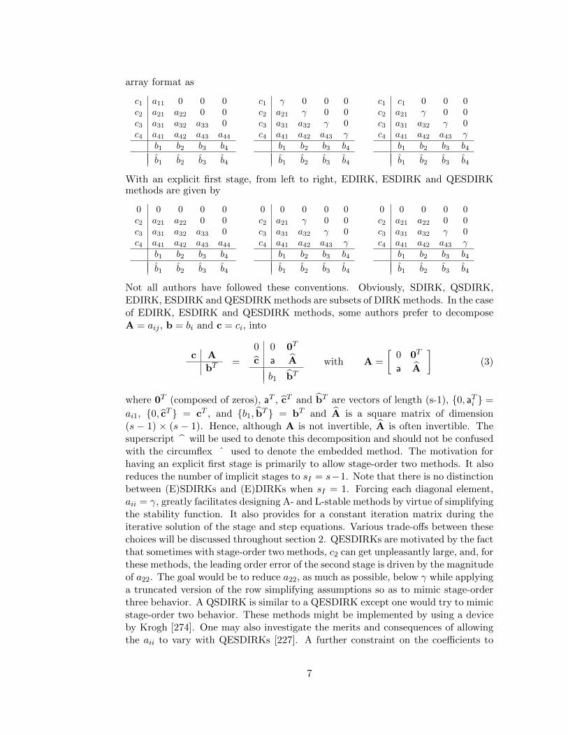
array format as
c1 a11 0 0 0c2 a21 a22 0 0c3 a31 a32 a33 0c4 a41 a42 a43 a44
b1 b2 b3 b4
b1 b2 b3 b4
c1 γ 0 0 0c2 a21 γ 0 0c3 a31 a32 γ 0c4 a41 a42 a43 γ
b1 b2 b3 b4
b1 b2 b3 b4
c1 c1 0 0 0c2 a21 γ 0 0c3 a31 a32 γ 0c4 a41 a42 a43 γ
b1 b2 b3 b4
b1 b2 b3 b4
With an explicit first stage, from left to right, EDIRK, ESDIRK and QESDIRKmethods are given by
0 0 0 0 0c2 a21 a22 0 0c3 a31 a32 a33 0c4 a41 a42 a43 a44
b1 b2 b3 b4
b1 b2 b3 b4
0 0 0 0 0c2 a21 γ 0 0c3 a31 a32 γ 0c4 a41 a42 a43 γ
b1 b2 b3 b4
b1 b2 b3 b4
0 0 0 0 0c2 a21 a22 0 0c3 a31 a32 γ 0c4 a41 a42 a43 γ
b1 b2 b3 b4
b1 b2 b3 b4
Not all authors have followed these conventions. Obviously, SDIRK, QSDIRK,EDIRK, ESDIRK and QESDIRK methods are subsets of DIRK methods. In the caseof EDIRK, ESDIRK and QESDIRK methods, some authors prefer to decomposeA = aij , b = bi and c = ci, into
c A
bT=
0 0 0T
c a A
b1 bTwith A =
[0 0T
a A
](3)
where 0T (composed of zeros), aT , cT and bT are vectors of length (s-1), {0, aTi } =
ai1, {0, cT } = cT , and {b1, bT } = bT and A is a square matrix of dimension(s − 1) × (s − 1). Hence, although A is not invertible, A is often invertible. Thesuperscript will be used to denote this decomposition and should not be confusedwith the circumflex ˆ used to denote the embedded method. The motivation forhaving an explicit first stage is primarily to allow stage-order two methods. It alsoreduces the number of implicit stages to sI = s−1. Note that there is no distinctionbetween (E)SDIRKs and (E)DIRKs when sI = 1. Forcing each diagonal element,aii = γ, greatly facilitates designing A- and L-stable methods by virtue of simplifyingthe stability function. It also provides for a constant iteration matrix during theiterative solution of the stage and step equations. Various trade-offs between thesechoices will be discussed throughout section 2. QESDIRKs are motivated by the factthat sometimes with stage-order two methods, c2 can get unpleasantly large, and, forthese methods, the leading order error of the second stage is driven by the magnitudeof a22. The goal would be to reduce a22, as much as possible, below γ while applyinga truncated version of the row simplifying assumptions so as to mimic stage-orderthree behavior. A QSDIRK is similar to a QESDIRK except one would try to mimicstage-order two behavior. These methods might be implemented by using a deviceby Krogh [274]. One may also investigate the merits and consequences of allowingthe aii to vary with QESDIRKs [227]. A further constraint on the coefficients to
7
these methods that is both simple and beneficial is the stiffly-accurate assumptionof Prothero and Robinson [340], asj = bj , implying cs = 1. Explicit first-stagemethods using the stiffly-accurate assumption are sometimes called first same as last(FSAL) methods [209, 324, 396, 397]. Albrecht [4] considers these composite linearmultistep methods. If a method has at least two identical values of ci, then it is calledconfluent, otherwise it is nonconfluent. Unlike reducible methods, methods that areDJ- (Dahlquist-Jeltsch [125]) or (H)S- (Hundsdorfer-Spijker [220]) irreducible cannotbe manipulated into an equivalent method having fewer stages.
To identify certain schemes derived in this paper, a nomenclature similar to thatoriginally devised by Dormand and Prince is followed [132,255]. For those schemesthat are given names, they will be named DIRKp(pI)sS[q]X x, where p is the orderof the main method, p is the order of the embedded method, I is included if internalerror-control is offered, s is the number of stages, S is some stability characterizationof the method, q is the stage-order of the method, X is used for any other importantcharacteristic of the method, and x distinguishes between family members of sometype of method.
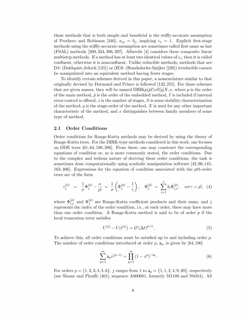
2.1 Order Conditions
Order conditions for Runge-Kutta methods may be derived by using the theory ofRunge-Kutta trees. For the DIRK-type methods considered in this work, one focuseson ODE trees [61, 64, 190, 286]. From these, one may construct the correspondingequations of condition or, as is more commonly stated, the order conditions. Dueto the complex and tedious nature of deriving these order conditions, the task issometimes done computationally using symbolic manipulation software [43,90,145,163, 406]. Expressions for the equation of condition associated with the pth-ordertrees are of the form
τ(p)j =
1
σΦ
(p)j −
α
p!=
1
σ
(Φ
(p)j −
1
γ
), Φ
(p)j =
s∑i=1
biΦ(p)i,j , ασγ = p!, (4)
where Φ(p)i,j and Φ
(p)j are Runge-Kutta coefficient products and their sums, and j
represents the index of the order condition, i.e., at each order, there may have morethan one order condition. A Runge-Kutta method is said to be of order p if thelocal truncation error satisfies
U [n] − U(t[n]) = O (∆t)p+1 . (5)
To achieve this, all order conditions must be satisfied up to and including order p.The number of order conditions introduced at order p, ap, is given by [64,190]
∞∑p=1
apx(p−1) =
∞∏p=1
(1− xp)−ap . (6)
For orders p = {1, 2, 3, 4, 5, 6}, j ranges from 1 to ap = {1, 1, 2, 4, 9, 20}, respectively(see Sloane and Plouffe [401]; sequence A000081, formerly M1180 and N0454). All
8
methods constructed later in this paper use the row-sum convention, Ae = c, wheree = {1, 1, · · · , 1}T . Verner [433] distinguishes four distinct types of order conditionsfor ODE contexts: quadrature, subquadrature, extended subquadrature and non-linear conditions. Moving from order p−1 to order p, one new quadrature conditionis introduced, (p− 2) for p ≥ 3 new subquadrature conditions and (2p−2− p+ 1) forp ≥ 4 new extended subquadrature conditions are added. Nonlinear order conditionsdo not arise until fifth-order and number ap − (2p−2), p ≥ 5.
Quadrature conditions allow solution of vector equations of the form y′(t) = f(t)and may be written at order k as
τ(k)Q =
1
(k − 1)!bTCk−1e− 1
k!, k = 1, 2, · · · , p, (7)
where C = diag(c) or Ce = c. Componentwise multiplication of two vectors, aand b will be denoted as a ∗ b. Powers of the vector c should be interpreted ascomponentwise multiplication. Hence c3 =c ∗ c ∗ c =C3e and c0 = e. Powers of theA-matrix are given by A0 = I, A1 = A and A2 = AA.
Trees associated with quadrature conditions are often referred to as bushy trees.Subquadrature conditions permit solution of linear, nonhomogeneous, vector equa-tions, y′(t) = Ay(t) + f(t), where A is a constant. They may be written at orderk + r as
τ(k+r)SQ =
1
(k − 1)!bTArCk−1e− 1
(k + r)!, k − 1, r ≥ 0, 1 ≤ k + r ≤ p. (8)
An important subset of the subquadrature conditions are the tall trees where k = 1;
τ(r+1)SQtall
= bTAre − 1/(r + 1)!, associated with the equation y′(t) = Ay(t). Setting
r = 0 recaptures the quadrature order conditions in (8). Extended subquadratureconditions extend these conditions to linear nonautonomous, nonhomogeneous vec-tor equations, y′(t) = A(t)y(t) + f(t). Defining K = k+
∑mj=0 kj and κi =
∑ij=0 kj ,
at order K they are
τ(K)ESQ =
1
σbTCk0−1ACk1−1 · · ·ACkm−1ACk−1e− α
K!, k, ki > 0 (9)
for 1 ≤ K ≤ p with σ = (k0 − 1)!(k1 − 1)! · · · (km − 1)!(k − 1)!, γ = (K − κm)(K −κm−1) · · · (K − κ0)K and α = K!/σγ. Setting k0 = k1 = · · · = km = 1 retrievesthe subquadrature conditions. All conditions not contained within these three cat-egories are nonlinear order conditions. Their general form, given by Verner [433], isquite complicated and will not be given here. Note that at lower orders, extendedsubquadrature conditions collapse into subquadrature conditions (ki = 1,m = r),and subquadrature conditions collapse into quadrature conditions (r = 0). Hence,even though the first nonlinear condition does not appear until fifth-order, lower-order methods retain their formal order on nonlinear problems. Appendix A listsRunge-Kutta order conditions up to sixth-order. Rather than increasing the orderof method by considering the order conditions at the next order, Farago et al. [146]attempt to achieve this using Richardson extrapolation.
9
Similar conditions apply to the embedded and dense output methods where band b(θ) (See §2.7) replace b in all of the preceeding expressions. Another importantaspect of order is the stage-order of a method, discussed in the following sections. Forthe stages, order conditions resemble those for the overall method (step conditionsversus stage conditions)
t(p)i,m =
1
σΥ
(p)i,m −
α
p!cpi , Υ
(p)i,m =
s∑j=1
aijΦ(p)j,m, ασγ = p!. (10)
2.2 Simplifying Assumptions
Simplifying assumptions are often made to facilitate the solution of Runge-Kuttaorder conditions and possibly to enforce higher stage-order. They were devised byButcher [59,60,129,190,193] based on the structure of Runge-Kutta trees and mayprovide insight into particular methods. The three common ones are
B(p) :s∑j=1
bick−1i =
1
k, k = 1, ..., p, (11)
C(η) :s∑j=1
aijck−1j =
ckik, k = 1, ..., η, (12)
D(ζ) :
s∑i=1
bick−1i aij =
bjk
(1− ckj ), k = 1, ..., ζ. (13)
A fourth simplifying assumption, E(η, ζ), is not needed for DIRK-type methods[129]. Recently, Khashin [258, 434] has given simplifying strategies substantiallydifferent from those given by Butcher. However, they are only likely to offer newinsight into methods having vastly different step and stage orders such as high-orderexplicit Runge-Kutta methods.
The first, (11), is related to the quadrature conditions. Enforcing B(p), (7),
forces τ(k)Q = 0, k = 1, 2, · · · , p for all orders up to and including p. Assumptions
C(η) and D(ζ) are sometimes referred to as the row and column simplifying as-sumptions, respectively. The stage-order of a Runge-Kutta method is the largestvalue of q such that B(q) and C(q) are both satisfied. As its name implies, stage-order is related to the order of accuracy of the intermediate stage values of theU -vector, Ui, and equals the lowest order amongst all stages. Stage-order stronglyinfluences the accuracy of methods when applied to stiff problems, boundary andsmoothness order-reduction, error-estimate quality and stage-value predictor qual-ity. While virtually all DIRK-type methods in the literature are at least stage-orderone by virtue of satisfying the row-sum condition Ae = c (Zlatev [466] does not),fewer satisfy C(2). This requires that a11 = 0 and forces a21 = a22. Hence, onlyEDIRK, ESDIRK and QESDIRK methods have the potential for a stage-order oftwo. It is impossible to satisfy C(3) for DIRK-type methods because of the second
stage where q(3)2 = 4a3
22/3, which implies that a22 = 0.
10
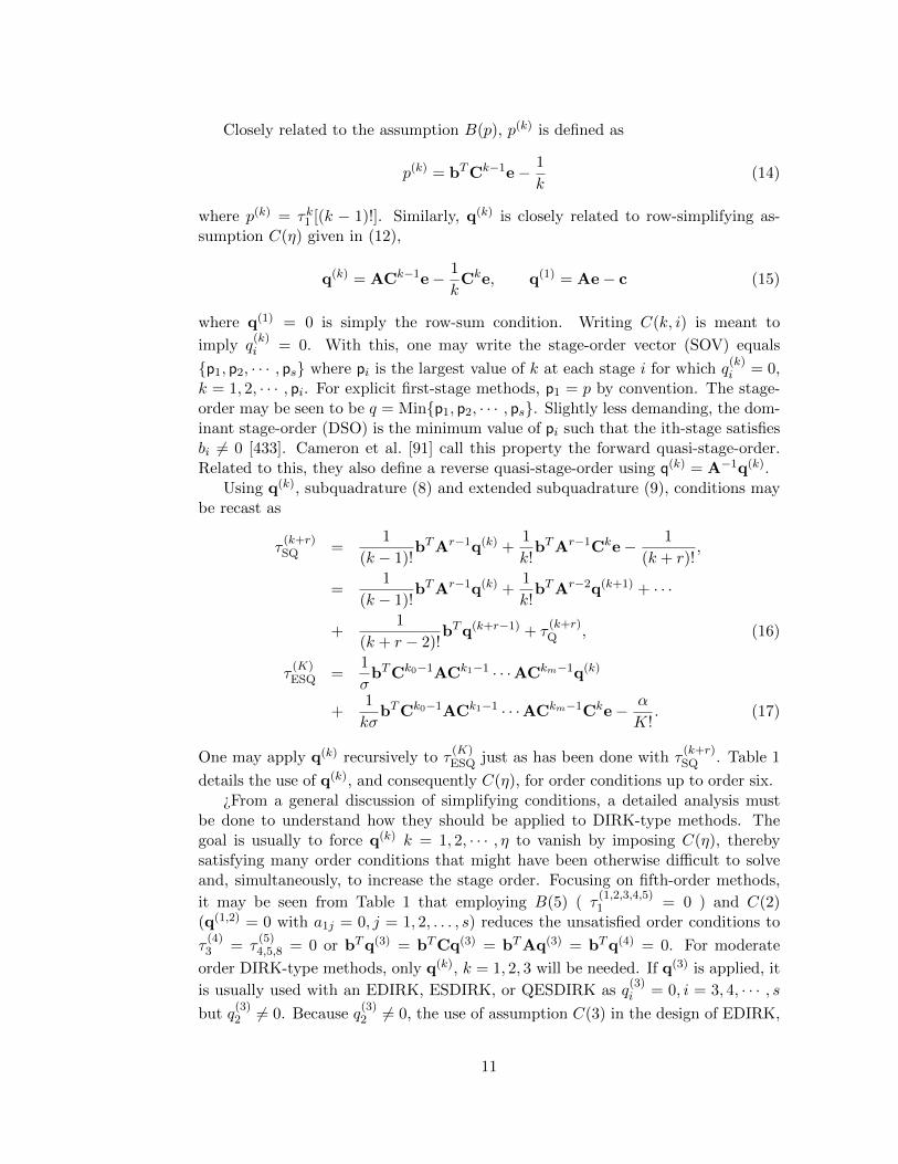
Closely related to the assumption B(p), p(k) is defined as
p(k) = bTCk−1e− 1
k(14)
where p(k) = τk1 [(k − 1)!]. Similarly, q(k) is closely related to row-simplifying as-sumption C(η) given in (12),
q(k) = ACk−1e− 1
kCke, q(1) = Ae− c (15)
where q(1) = 0 is simply the row-sum condition. Writing C(k, i) is meant to
imply q(k)i = 0. With this, one may write the stage-order vector (SOV) equals
{p1, p2, · · · , ps} where pi is the largest value of k at each stage i for which q(k)i = 0,
k = 1, 2, · · · , pi. For explicit first-stage methods, p1 = p by convention. The stage-order may be seen to be q = Min{p1, p2, · · · , ps}. Slightly less demanding, the dom-inant stage-order (DSO) is the minimum value of pi such that the ith-stage satisfiesbi 6= 0 [433]. Cameron et al. [91] call this property the forward quasi-stage-order.Related to this, they also define a reverse quasi-stage-order using q(k) = A−1q(k).
Using q(k), subquadrature (8) and extended subquadrature (9), conditions maybe recast as
τ(k+r)SQ =
1
(k − 1)!bTAr−1q(k) +
1
k!bTAr−1Cke− 1
(k + r)!,
=1
(k − 1)!bTAr−1q(k) +
1
k!bTAr−2q(k+1) + · · ·
+1
(k + r − 2)!bTq(k+r−1) + τ
(k+r)Q , (16)
τ(K)ESQ =
1
σbTCk0−1ACk1−1 · · ·ACkm−1q(k)
+1
kσbTCk0−1ACk1−1 · · ·ACkm−1Cke− α
K!. (17)
One may apply q(k) recursively to τ(K)ESQ just as has been done with τ
(k+r)SQ . Table 1
details the use of q(k), and consequently C(η), for order conditions up to order six.¿From a general discussion of simplifying conditions, a detailed analysis must
be done to understand how they should be applied to DIRK-type methods. Thegoal is usually to force q(k) k = 1, 2, · · · , η to vanish by imposing C(η), therebysatisfying many order conditions that might have been otherwise difficult to solveand, simultaneously, to increase the stage order. Focusing on fifth-order methods,
it may be seen from Table 1 that employing B(5) ( τ(1,2,3,4,5)1 = 0 ) and C(2)
(q(1,2) = 0 with a1j = 0, j = 1, 2, . . . , s) reduces the unsatisfied order conditions to
τ(4)3 = τ
(5)4,5,8 = 0 or bTq(3) = bTCq(3) = bTAq(3) = bTq(4) = 0. For moderate
order DIRK-type methods, only q(k), k = 1, 2, 3 will be needed. If q(3) is applied, it
is usually used with an EDIRK, ESDIRK, or QESDIRK as q(3)i = 0, i = 3, 4, · · · , s
but q(3)2 6= 0. Because q
(3)2 6= 0, the use of assumption C(3) in the design of EDIRK,
11
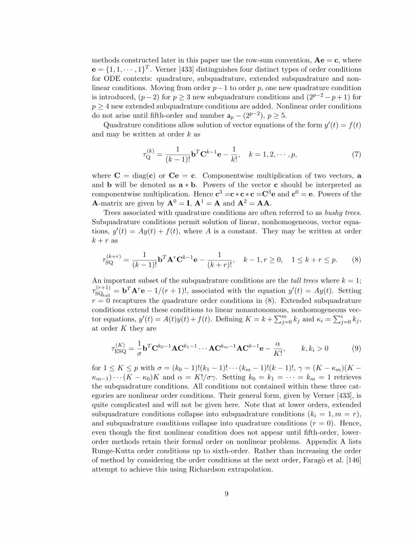
Table 1. Order conditions expressed using q(k), k = 2, 3, 4, 5 up to sixth-order for
Runge-Kutta methods. Bushy tree order conditions τ(l)1 , l = 1, 2, · · · , 6 are not
included. Order conditions are denoted as to whether they are subquadrature (SQ),extended subquadrature (ESQ) or nonlinear (NL).
SQ τ(3)2 = bTq(2) + τ
(3)1
ESQ τ(4)2 = bTCq(2) + 3τ
(4)1
SQ τ(4)3 = 1
2bTq(3) + τ(4)1
SQ τ(4)4 = bTAq(2) + τ
(4)3
ESQ τ(5)2 = 1
2bTC2q(2) + 6τ(5)1
NL τ(5)3 = 1
2bT(q(2)
)2+ 1
2bTC2q(2) + 3τ(5)1
ESQ τ(5)4 = 1
2bTCq(3) + 4τ(5)1
SQ τ(5)5 = 1
6bTq(4) + τ(5)1
ESQ τ(5)6 = bTCAq(2) + τ
(5)4
ESQ τ(5)7 = bTACq(2) + 3τ
(5)5
SQ τ(5)8 = 1
2bTAq(3) + τ(5)5
SQ τ(5)9 = bTAAq(2) + τ
(5)8
ESQ τ(6)2 = 1
6bTC3q(2) + 10τ(6)1
NL τ(6)3 = 1
2bTC(q(2)
)2+ 1
2bTC3q(2) + 15τ(6)1
ESQ τ(6)4 = 1
4bTC2q(3) + 10τ(6)1
NL τ(6)5 = 1
2bTQ(3)q(2) + 16bTC3q(2) + τ
(6)4
ESQ τ(6)6 = 1
6bTCq(4) + 5τ(6)1
SQ τ(6)7 = 1
24bTq(5) + τ(6)1
ESQ τ(6)8 = 1
2bTC2Aq(2) + τ(6)4
NL τ(6)9 = bTQ(2)Aq(2) + 1
2bTQ(2)q(3) + 16bTC3q(2) + τ
(6)8
ESQ τ(6)10 = bTCACq(2) + 3τ
(6)6
ESQ τ(6)11 = 1
2bTAC2q(2) + 6τ(6)7
NL τ(6)12 = 1
2bTA(q(2)
)2+ 1
2bTAC2q(2) + 3τ(6)7
ESQ τ(6)13 = 1
2bTCAq(3) + τ(6)6
ESQ τ(6)14 = 1
2bTACq(3) + 4τ(6)7
SQ τ(6)15 = 1
6bTAq(4) + τ(6)7
ESQ τ(6)16 = bTCAAq(2) + τ
(6)13
ESQ τ(6)17 = bTACAq(2) + τ
(6)14
ESQ τ(6)18 = bTAACq(2) + 3τ
(6)15
SQ τ(6)19 = 1
2bTAAq(3) + τ(6)15
SQ τ(6)20 = bTAAAq(2) + τ
(6)19
12
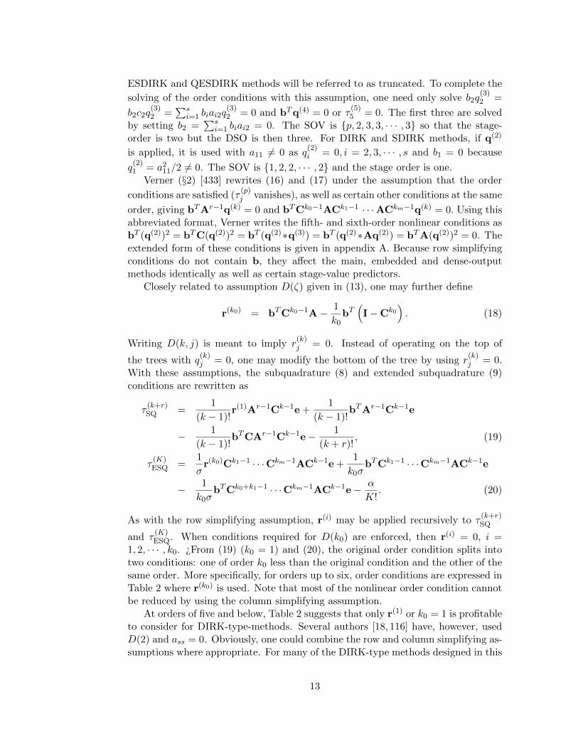
ESDIRK and QESDIRK methods will be referred to as truncated. To complete the
solving of the order conditions with this assumption, one need only solve b2q(3)2 =
b2c2q(3)2 =
∑si=1 biai2q
(3)2 = 0 and bTq(4) = 0 or τ
(5)5 = 0. The first three are solved
by setting b2 =∑s
i=1 biai2 = 0. The SOV is {p, 2, 3, 3, · · · , 3} so that the stage-order is two but the DSO is then three. For DIRK and SDIRK methods, if q(2)
is applied, it is used with a11 6= 0 as q(2)i = 0, i = 2, 3, · · · , s and b1 = 0 because
q(2)1 = a2
11/2 6= 0. The SOV is {1, 2, 2, · · · , 2} and the stage order is one.Verner (§2) [433] rewrites (16) and (17) under the assumption that the order
conditions are satisfied (τ(p)j vanishes), as well as certain other conditions at the same
order, giving bTAr−1q(k) = 0 and bTCk0−1ACk1−1 · · ·ACkm−1q(k) = 0. Using thisabbreviated format, Verner writes the fifth- and sixth-order nonlinear conditions asbT (q(2))2 = bTC(q(2))2 = bT (q(2)∗q(3)) = bT (q(2)∗Aq(2)) = bTA(q(2))2 = 0. Theextended form of these conditions is given in appendix A. Because row simplifyingconditions do not contain b, they affect the main, embedded and dense-outputmethods identically as well as certain stage-value predictors.
Closely related to assumption D(ζ) given in (13), one may further define
r(k0) = bTCk0−1A− 1
k0bT(I−Ck0
). (18)
Writing D(k, j) is meant to imply r(k)j = 0. Instead of operating on the top of
the trees with q(k)j = 0, one may modify the bottom of the tree by using r
(k)j = 0.
With these assumptions, the subquadrature (8) and extended subquadrature (9)conditions are rewritten as
τ(k+r)SQ =
1
(k − 1)!r(1)Ar−1Ck−1e +
1
(k − 1)!bTAr−1Ck−1e
− 1
(k − 1)!bTCAr−1Ck−1e− 1
(k + r)!, (19)
τ(K)ESQ =
1
σr(k0)Ck1−1 · · ·Ckm−1ACk−1e +
1
k0σbTCk1−1 · · ·Ckm−1ACk−1e
− 1
k0σbTCk0+k1−1 · · ·Ckm−1ACk−1e− α
K!. (20)
As with the row simplifying assumption, r(i) may be applied recursively to τ(k+r)SQ
and τ(K)ESQ. When conditions required for D(k0) are enforced, then r(i) = 0, i =
1, 2, · · · , k0. ¿From (19) (k0 = 1) and (20), the original order condition splits intotwo conditions: one of order k0 less than the original condition and the other of thesame order. More specifically, for orders up to six, order conditions are expressed inTable 2 where r(k0) is used. Note that most of the nonlinear order condition cannotbe reduced by using the column simplifying assumption.
At orders of five and below, Table 2 suggests that only r(1) or k0 = 1 is profitableto consider for DIRK-type-methods. Several authors [18, 116] have, however, usedD(2) and ass = 0. Obviously, one could combine the row and column simplifying as-sumptions where appropriate. For many of the DIRK-type methods designed in this
13
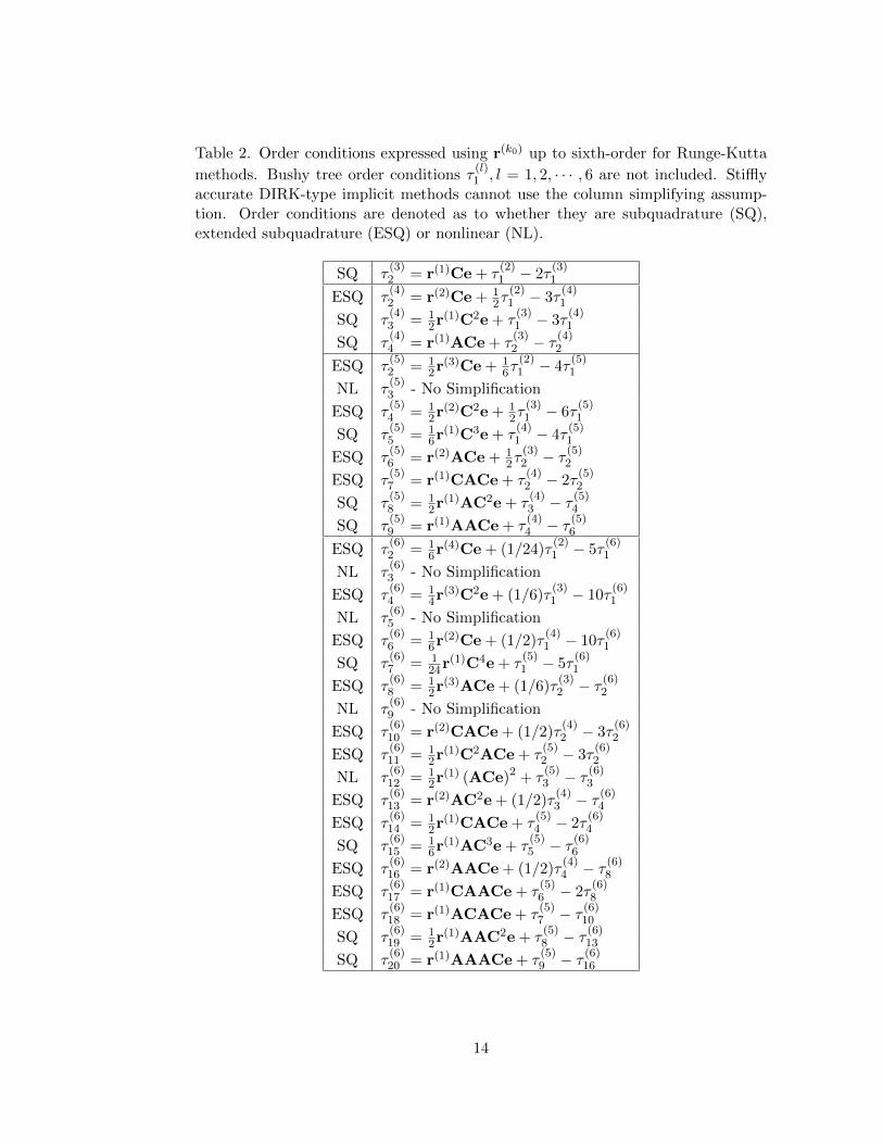
Table 2. Order conditions expressed using r(k0) up to sixth-order for Runge-Kutta
methods. Bushy tree order conditions τ(l)1 , l = 1, 2, · · · , 6 are not included. Stiffly
accurate DIRK-type implicit methods cannot use the column simplifying assump-tion. Order conditions are denoted as to whether they are subquadrature (SQ),extended subquadrature (ESQ) or nonlinear (NL).
SQ τ(3)2 = r(1)Ce + τ
(2)1 − 2τ
(3)1
ESQ τ(4)2 = r(2)Ce + 1
2τ(2)1 − 3τ
(4)1
SQ τ(4)3 = 1
2r(1)C2e + τ(3)1 − 3τ
(4)1
SQ τ(4)4 = r(1)ACe + τ
(3)2 − τ (4)
2
ESQ τ(5)2 = 1
2r(3)Ce + 16τ
(2)1 − 4τ
(5)1
NL τ(5)3 - No Simplification
ESQ τ(5)4 = 1
2r(2)C2e + 12τ
(3)1 − 6τ
(5)1
SQ τ(5)5 = 1
6r(1)C3e + τ(4)1 − 4τ
(5)1
ESQ τ(5)6 = r(2)ACe + 1
2τ(3)2 − τ (5)
2
ESQ τ(5)7 = r(1)CACe + τ
(4)2 − 2τ
(5)2
SQ τ(5)8 = 1
2r(1)AC2e + τ(4)3 − τ (5)
4
SQ τ(5)9 = r(1)AACe + τ
(4)4 − τ (5)
6
ESQ τ(6)2 = 1
6r(4)Ce + (1/24)τ(2)1 − 5τ
(6)1
NL τ(6)3 - No Simplification
ESQ τ(6)4 = 1
4r(3)C2e + (1/6)τ(3)1 − 10τ
(6)1
NL τ(6)5 - No Simplification
ESQ τ(6)6 = 1
6r(2)Ce + (1/2)τ(4)1 − 10τ
(6)1
SQ τ(6)7 = 1
24r(1)C4e + τ(5)1 − 5τ
(6)1
ESQ τ(6)8 = 1
2r(3)ACe + (1/6)τ(3)2 − τ (6)
2
NL τ(6)9 - No Simplification
ESQ τ(6)10 = r(2)CACe + (1/2)τ
(4)2 − 3τ
(6)2
ESQ τ(6)11 = 1
2r(1)C2ACe + τ(5)2 − 3τ
(6)2
NL τ(6)12 = 1
2r(1) (ACe)2 + τ(5)3 − τ (6)
3
ESQ τ(6)13 = r(2)AC2e + (1/2)τ
(4)3 − τ (6)
4
ESQ τ(6)14 = 1
2r(1)CACe + τ(5)4 − 2τ
(6)4
SQ τ(6)15 = 1
6r(1)AC3e + τ(5)5 − τ (6)
6
ESQ τ(6)16 = r(2)AACe + (1/2)τ
(4)4 − τ (6)
8
ESQ τ(6)17 = r(1)CAACe + τ
(5)6 − 2τ
(6)8
ESQ τ(6)18 = r(1)ACACe + τ
(5)7 − τ (6)
10
SQ τ(6)19 = 1
2r(1)AAC2e + τ(5)8 − τ (6)
13
SQ τ(6)20 = r(1)AAACe + τ
(5)9 − τ (6)
16
14
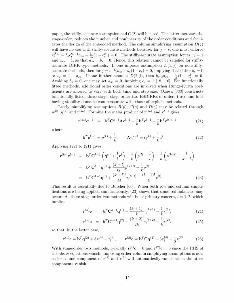
paper, the stiffly-accurate assumption and C(2) will be used. The latter increases thestage-order, reduces the number and nonlinearity of the order conditions and facili-tates the design of the embedded method. The column simplifying assumption D(ζ)will have no use with stiffly-accurate methods because, for j = s, one must enforce
r(k0)s = bsc
k0−1s ass − bs
k0(1 − ck0s ) = 0. The stiffly-accurate assumption forces cs = 1
and ass = bs so that ass = bs = 0. Hence, this relation cannot be satisfied for stiffly-accurate DIRK-type methods. If one imposes assumption D(1, j) on nonstiffly-accurate methods, then for j = s, bsass− bs(1− cs) = 0, implying that either bs = 0or cs = 1 − ass. If one further assumes D(2, j), then bscsass − bs
2 (1 − c2s) = 0.
Avoiding bs = 0, one may set ass = 0, implying cs = 1 [18, 116]. For functionallyfitted methods, additional order conditions are involved when Runge-Kutta coef-ficients are allowed to vary with both time and step size. Ozawa [333] constructsfunctionally fitted, three-stage, stage-order two ESDIRKs of orders three and fourhaving stability domains commensurate with those of explicit methods.
Lastly, simplifying assumptions B(p), C(η) and D(ζ) may be related throughp(k), q(k) and r(k0). Forming the scalar product of r(k0) and cl−1 gives
r(k0)cl−1 = bTCk−1Acl−1 − 1
kbT cl−1 +
1
kbT ck+l−1 (21)
where
bT ck−1 = p(k) +1
k, Ack−1 = q(k) +
1
kck. (22)
Applying (22) to (21) gives
r(k0)cl−1 = bTCk−1
(q(l) +
1
lcl)− 1
k
(p(l) +
1
l
)+
1
k
(p(k+l) +
1
k + l
)= bTCk−1q(l) +
(k + l)
klp(k+l) − 1
kp(l)
= bTCk−1q(l) +(k + l)!
klτ
(k+l)1 − (l − 1)!
kτ
(l)1 . (23)
This result is essentially due to Butcher [60]. When both row and column simpli-fications are being applied simultaneously, (23) shows that some redundancies mayoccur. As these stage-order two methods will be of primary concern, l = 1, 2, whichimplies
r(k)e = bTCk−1q(1) +(k + 1)!
kτ
(k+1)1 − 1
kτ
(1)1 , (24)
r(k)c = bTCk−1q(2) +(k + 2)!
2kτ
(k+2)1 − 1
kτ
(2)1 . (25)
so that, in the latter case,
r(1)c = bTq(2) + 3τ(3)1 − τ (2)
1 , r(2)c = bTCq(2) + 6τ(4)1 − 1
2τ
(2)1 . (26)
With stage-order two methods, typically r(1)c = 0 and r(2)c = 0 since the RHS ofthe above equations vanish. Imposing either column simplifying assumptions is noweasier as one component of r(1) and r(2) will automatically vanish when the othercomponents vanish.
15
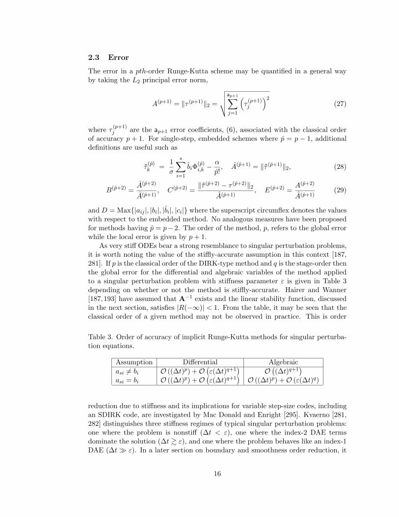
2.3 Error
The error in a pth-order Runge-Kutta scheme may be quantified in a general wayby taking the L2 principal error norm,
A(p+1) = ‖τ (p+1)‖2 =
√√√√ap+1∑j=1
(τ
(p+1)j
)2(27)
where τ(p+1)j are the ap+1 error coefficients, (6), associated with the classical order
of accuracy p + 1. For single-step, embedded schemes where p = p − 1, additionaldefinitions are useful such as
τ(p)k =
1
σ
s∑i=1
biΦ(p)i,k −
α
p!, A(p+1) = ‖τ (p+1)‖2, (28)
B(p+2) =A(p+2)
A(p+1), C(p+2) =
‖τ (p+2) − τ (p+2)‖2A(p+1)
, E(p+2) =A(p+2)
A(p+1)(29)
and D = Max{|aij |, |bi|, |bi|, |ci|} where the superscript circumflex denotes the valueswith respect to the embedded method. No analogous measures have been proposedfor methods having p = p− 2. The order of the method, p, refers to the global errorwhile the local error is given by p+ 1.
As very stiff ODEs bear a strong resemblance to singular perturbation problems,it is worth noting the value of the stiffly-accurate assumption in this context [187,281]. If p is the classical order of the DIRK-type method and q is the stage-order thenthe global error for the differential and algebraic variables of the method appliedto a singular perturbation problem with stiffness parameter ε is given in Table 3depending on whether or not the method is stiffly-accurate. Hairer and Wanner[187,193] have assumed that A−1 exists and the linear stability function, discussedin the next section, satisfies |R(−∞)| < 1. From the table, it may be seen that theclassical order of a given method may not be observed in practice. This is order
Table 3. Order of accuracy of implicit Runge-Kutta methods for singular perturba-tion equations.
Assumption Differential Algebraic
asi 6= bi O ((∆t)p) +O(ε(∆t)q+1
)O((∆t)q+1
)asi = bi O ((∆t)p) +O
(ε(∆t)q+1
)O ((∆t)p) +O (ε(∆t)q)
reduction due to stiffness and its implications for variable step-size codes, includingan SDIRK code, are investigated by Mac Donald and Enright [295]. Kvaerno [281,282] distinguishes three stiffness regimes of typical singular perturbation problems:one where the problem is nonstiff (∆t < ε), one where the index-2 DAE termsdominate the solution (∆t & ε), and one where the problem behaves like an index-1DAE (∆t� ε). In a later section on boundary and smoothness order reduction, it
16
will be seen that order reduction may also occur due to spatial boundary conditionsin a discretized PDE or nonsmooth coefficients contained within the right hand side(RHS) of the ODEs. The worst occurrences of this order reduction will result inglobal convergence rates of the minimum between p and q + 1. Several detailedconvergence studies [139,320] are also available.
2.4 Linear Stability
Linear stability of DIRK-type methods applied to ODEs is studied based on theequation U ′ = λU by using the stabilty function
R(z) =P (z)
Q(z)=
Det[I− zA + ze⊗ bT
]Det [I− zA]
= 1 + zbT [I− zA]−1 e, (30)
where I is the identity matrix and z = λ∆t. Similar expressions may be writtenfor the embedded and dense output methods by simply replacing b with b andb(θ), respectively. If t0 = 0 and U(t0) = 1, then after one step, U = exp(λ∆t) =exp(z). Therefore, one would like R(z) to approximate exp(z). The motivation forstudying this simple equation when actually trying to solve (1) is based on a two-partsimplification [412]. One first linearizes (1) to U ′ = AU where A is the Jacobian∂F/∂U at any point t∗ belonging to the time interval under consideration [69].Next, one selects an eigenvalue λ, belonging to the spectrum of A, where λ maybe complex. On occasions, these simplifications may break down and render linearstability insufficient. Both numerator and denominator of the stability function arepolynomials of degree, deg ≤ s. An explicit first stage reduces the degree of thedenominator by one. A method is called A-stable and its stability function is calledA-acceptable if |R(z)| ≤ 1 for <(z) ≤ 0. If <(z) ≤ 0, then the linear autonomousproblem U ′ = λU is dissipative in an inner product norm, i.e., for two differentsolutions ||U(t + ∆t) − U(t + ∆t)|| ≤ ||U(t) − U(t)||. The inner product normof a vector x is defined as ||x|| =
√< x, x >. A common alternative expression
is obtained by differentiating the separation distance between the two solutionsand requiring that it never increase; that is d
dt ||U(t)− U(t)||2 ≤ 0 or ||F (t, U(t))−F (t, U(t)), U(t)−U(t)|| ≤ 0. The tilde solution may be thought of as a perturbationof the original solution due to truncation, round-off and iteration errors [415]. A-stability then implies the unconditional (all step-sizes ∆t > 0) contractivity of thecorresponding numerical solution in an inner product norm, ||U [n+1] − U [n+1]|| ≤||U [n]−U [n]|| [267]. Hence, the radius of contractivity is rL2 = ∞, where L denotesa linear problem and the subscript 2 denotes the norm. If one attempts to extendunconditional contractivity of Runge-Kutta methods applied to linear autonomousproblems to an arbitrary norm, which includes the max norm with rL∞= ∞, thenR(z) must be absolutely monotonic for z on the entire negative real axis, −∞ ≤z ≤ 0, and, consequently, the order of accuracy may not exceed one [408]. If, inaddition to A-stability, R(z)z→−∞ = 0, then the method is called L-stable, andits stability function is called L-acceptable. L-acceptable stability functions havedeg Q(z) > deg P (z). Intermediate between A- and L-stability is what Crouzeix[120,121,123] terms strong A-stability. This requires that a method be A-stable and
17
R(z)z→−∞ < 1 which gives the method a desirable error growth function [170,171].Less restrictive measures of linear stability may also be considered [193, 286, 457].A(α)-stable methods provide |R(z)| ≤ 1 for all z in a sector of ±α radians aboveand below the negative real axis, −∞ ≤ z ≤ 0, within the complex left half-plane(LHP). If α = π/2, then the method is simply A-stable. If that angle includesα = 0, the negative real axis, then the method is called A0-stable. Methods thatare both A(α)-stable and have R(z)z→−∞ = 0 are termed L(α)-stable. A simpleway to assist in achieving L-stability is to set ps = 0 in (31) by using the stiffly-accurate assumption, asj = bj [340], which reduces the deg P (z) from s to s − 1.The stiffly-accurate assumption forces U [n+1] to be computed implicitly, while alsoincreasing the convergence rate (see Table 3) on stiff and DAE problems. Lastly, astability function is said to be P-stable if |R(iν)| = 1 where i =
√−1 and ν is a real
number [152,212].Given the stability function, (30), then
Rm,n(z) =P (z)
Q(z)=
∑mi=0 piz
i∑nj=0 qjz
j=
∑si=0 piz
i∏sj=1 (1− ajjz)
(31)
where pi and qi are real. Nørsett and Wolfbrandt [318,452] show that the maximumorder of approximation to exp(z) using Rm,n(z) is m+1 if all poles are real. Appliedto SDIRKs and ESDIRKs, this implies p ≤ sI + 1. To better understand the max-imum order of approximation for A-acceptable approximations to exp(z), Wanneret al. [70, 227, 316, 317, 443, 444] introduced order stars where the order star of anapproximation to the exponential is given by R(z)/ exp(z). Shirkov [386] attemptsto design L-stable DIRK methods having p = s, s = 1, 2, 3, 4 with “second-orderdamped” (SOD), i.e., deg Q(z) = deg P (z) + 2 or p = sI + 2 rather than the morecommon deg Q(z) = deg P (z) + 1. ¿From Nørsett [308, 309] and Crouzeix [120],SDIRK methods of order p = {2, 3, 4} and s = {1, 2, 3} have been derived. The twohigher-order, A-stable methods are shown to be unique but a four-stage, fifth-ordermethod is impossible. Nørsett and Wolfbrandt state that a DIRK with p = 5 ands = 4 must have two distinct values of aii. Cooper and Sayfy [116] and Shintani andYoshida [385] derive A-stable SDIRK methods having p = 5 and s = 5. Relaxingthe requirement of identical diagonal coefficients, Cooper and Sayfy [116] derive anA-stable DIRK with p = 6 and s = 6, but the last stage is computed explicitly asa66 = 0. It is unlikely that an A-stable p = 6, s = 6 SDIRK exists. Methods havingp = 5 and s = 4 [18], p = 5 and s = 5 [266], p = 6 and s = 5 [18] have also beenderived, yet none are A-stable. Al-Rabeh [18] shows that the maximum order ofan s-stage, nonconfluent DIRK with nonzero weights cannot exceed s+ 1 and doesthis only for 1 ≤ s ≤ 5. Bales et al. [30] prove that for Q(z) =
∏sIi=1 (1− aiiz), if
aii ≥ 1/2, i = 1, 2, · · · , sI and R(z) is at least an order sI approximation to theexponential, then R(z) is A0-acceptable. Associated with each stability function isan error constant, C, defined by [262, 278, 395] exp(z) − R(z) = Czp+1 + O(zp+2),where R(z) is a pth-order approximant to the exponential. Burrage [50] and Wan-ner [442] note that when simplifying assumptions are applied to the method, theerror constant bears a close resemblance to the error constant of the entire Runge-Kutta method. In low stage-order methods, this correlation is generally lost. As
18
the error is indicative of the error near z = 0, a minimum error constant may notbe minimal for |z| � 0 [395]. Orel [326] proves that the minimum error constant ofany approximant to the exponential having only real poles has all poles equal. Iser-les and Nørsett [227] suggest that it may be profitable to consider DIRK methodsrather than SDIRK methods. They ask whether more methods may be generatedthat are A-stable and whether certain order barriers might be broken by allowingthe aii to vary. The work of Orel [326] and Keeling [253] suggests that there is nobenefit to permitting distinct, nonzero, diagonal entries in Q(z). Shirobokov seeksto minimize the value of the error constant of SDIRK [387] and DIRK [388–391]methods along a finite interval of the negative real-axis beginning at the origin. In alater paper, Shirobokov [392–394] seeks to minimize the magnitude of |R(z)−exp(z)|within the class of fourth-order accurate A0-stable DIRK methods. Kalitkin andPoshivaylo [250] seek to optimize implicit Runge-Kutta methods by considering theinverse stability function of an explicit Runge-Kutta method.
Limiting the discussion to SDIRKs and ESDIRKs, one may derive some usefulanalytical results regarding R(z) for A-stable methods in cases where the order ofthe method p and the number of implicit stages are related by sI ≤ p ≤ sI + 1.For L-stable methods, this becomes sI − 1 ≤ p ≤ sI . Nørsett [309, 311] and others[50,123,193,442] derive a compact expression for the SDIRK and ESDIRK stabilityfunction in terms of Laguerre polynomials. Using the definitions of the Laguerrepolynomials and their mth-derivatives,
Ls(x) =
s∑k=0
(s
k
)(−x)k
k!, L(m)
s (x) =s−m∑k=0
(s
k +m
)(−1)k+mxk
k!, (32)
where (s
k
)=
s!
(s− k)!k!, (33)
one may write
P (z) =
sI∑j=0
pjzj = (−1)sI
sI∑j=0
L(sI−j)sI
(1
γ
)(γz)j
=
sI∑j=0
zjj∑
k=0
(sIk
)(−γ)k
(j − k)!, (34)
Q(z) = (1− γz)sI =
sI∑k=0
qkzk =
sI∑k=0
(sIk
)(−γ)kzk (35)
with error constant
C =γsI (−1)sI+1
(sI + 1)L
(1)sI+1
(1
γ
)=
1
sI + 1
sI∑k=0
(sI + 1
k + 1
)(−γ)sI−k
k!. (36)
These results merit a quick explanation. The expression for Q(z) follows directlyfrom its definition, Q(z) = Det [I− zA], and the diagonal structure of A. From
19
[227], P (z) is defined by
P (z) =m∑j=0
pjzj = (1− γz)n exp(z) +O
(zm+1
)(37)
since R(z) is a restricted approximant to the exponential. Matching terms afterexpanding (1 − γz)n exp(z) in a series provides the form of P (z). This result maythen be recast in terms of Laguerre polynomials.
Forcing the error constant to vanish gives the γ for which the stability functionis an (sI + 1)th-order approximation to exp(z) [309]. If one restricts this to caseswhere deg P (z) + 1 = deg Q(z) and sI − 1 ≤ p ≤ sI , then the method will haveR(−∞) = 0. In this case, psI = 0 and
P (z) =
sI−1∑j=0
pjzj = (−1)sI
sI−1∑j=0
L(sI−j)sI
(1
γ
)(γz)j
=
sI−1∑j=0
zjj∑
k=0
(sIk
)(−γ)k
(j − k)!(38)
with psI = C = 0
C = psI = (−γ)sILsI
(1
γ
)=
sI∑k=0
(sIk
)(−γ)sI−k
k!=
sI∑k=0
(sIk
)(−γ)k
(sI − k)!. (39)
Higher-order error terms are given by Koto [262]. Butcher [67] also considers thecase p = s − 2. Concepcion [110] gives the necessary and sufficient conditions forthe A-acceptability of Rk−1,k(z) approximates to the exponential having a singlereal root, γ−1 (aii = γ). This is relevant to L-stable SDIRKs and ESDIRKs. Giventhe form of the stability function, one may enforce A- or I-stability. A Runge-Kutta method is imaginary axis or I-stable if |R(z)| ≤ 1 for <(z) = 0. Alt [20]determines that if R(z) has no poles in the complex LHP and the stability functionis I-acceptable (the Runge-Kutta method is I-stable) then the method is A-stable.An analytic stability function for DIRK-type methods simply requires that aii ≥ 0.Nørsett [310] devises the E-polynomial to test for I-stability,
E(y) = Q(+iy)Q(−iy)− P (+iy)P (−iy)
= E0 + E2 y2 + · · ·+ E2s y
2s =
s∑j=0
E2j y2j (40)
where i =√−1. Contemporaries of Nørsett; Alt [19, 20, 22], Crouzeix [120, 121],
Kurdi [278] and Miller [299] use the identical principle in a slightly different form:|R(iy)| ≤ 1 for all real y. In general for DIRK-type methods, Q(+iy)Q(−iy) =∏sIj=1
[1 + (ajjy)2
]; however, for SDIRKs and ESDIRKs, Q(+iy)Q(−iy) = [1 +
(γy)2]sI . I-stability requires that E(y) ≥ 0 for all values of real y, which requiresE(y) to have only imaginary roots. It is sufficient, but not necessary, to have E2j ≥
20
0, j = 1, 2, · · · , s. For order p ≥ 2j, E2j = 0. First-stage explicit methods reduce thedegree of Q(z) by one, while stiffly-accurate methods reduce the degree of P (z) byone by forcing ps = 0. Hence, E2s = 0. Further, if L-stability is desired, then psI−1
must also vanish. Related but slightly different, Cooper and Sayfy [116] analyseA-stability for DIRK-type methods with one or more aii = 0. This may cause onestage value to be updated explicitly and may result in severe internal instabilityon stiff problems. Al-Rabeh [17] investigates the requirements for A-stability whenp = s and all diagonal coefficients are not equal. An alternative, yet less practical,approach to establishing I- and A-stability is given by Scherer and Wendler [182,191, 303, 358, 359]. Defining C = A − 1
2ebT and Q = {e,Ae, · · · ,As−1e}, then anecessary and sufficient condition for I-stability is that there exists a symmetricmatrix R such that Re = b and QT (RC + CTR)Q are non-negative definite. If, inaddition, QTRQ is non-negative definite, then the method is also A-stable. Theseconditions may be simplified a bit in cases where the stability function is minimal bysetting Q = I. Minimality is a stronger requirement on a method than irreducibilityand requires that deg P (z) and deg Q(z) are not both less than s [358]. A- andL-stable, first-stage explicit DIRK-type methods are not minimal. Note that forQ = I and R = B = diag(b), then (RC+CTR) equals the algebraic stability matrixM given by (47).
With the E-polynomial, one may establish a priori the bounds on γ that willresult in either A-stable or L-stable methods [50, 193, 311] provided that p ≈ s.These bounds are given in Tables 4 and 5. Entries in the tables arise via severaldifferent avenues. All A-stable values of γ in Table 4 entries, except γ = (3 +√
3)/6, correspond to roots of E2s or E2jmin where jmin is the minimum value thatcorresponds to a nonzero value of E2j . While these two criteria are not sufficient toensure that E(y) ≥ 0, they correspond to the observed values of γ in Table 4. The
γ = (3 +√
3)/6 entry results from satisfying order condition τ(3)2 . Ranges of γ for
A-stability are those where both E2s or E2jmin remain non-negative. For s odd, if aroot of E2jmin is in this range, then order p = s + 1 can be achieved. No A-stablemethods were found for 9 ≥ sI ≥ 20.
Finding L-stable values of γ, shown in Table 5, involves the values for the roots ofpsI , E2s, E2jmin and the roots to the discriminant of E(y). Since E2s = γ2s, E2s willremain positive for all positive values of γ. Boundaries in the range of γ correspondto a root of either E2jmin or the discriminant of E(y). Some care should be taken atthe values of γ which separate L-stable from non-L-stable methods as some boundarypoints have |R(iy)| = 1 at discrete points on the imaginary axis [170]. Aggregatingand sorting these roots according to their magnitude, if E(y) ≥ 0 between twoadjacent roots, then the method is L-stable for values of γ between these adjacentroot values. Further, if a root of psI resides within this range, then the order of themethod is p = s. An alternative procedure to determine I-stability for any DIRK-type method is to simply compute all roots of E(y) for a given value of γ and ensurethat all roots are imaginary. No L-stable methods were found for 12 ≥ sI ≥ 20.
Rather than seek L-stable stability functions given in (31) by setting m = sI − 1and n = sI , one may seek stability functions where m = sI − 2 and n = sI ,zR(z)z→−∞ = 0, in hopes of having stronger damping of stiff scaled eigenvalues.
21
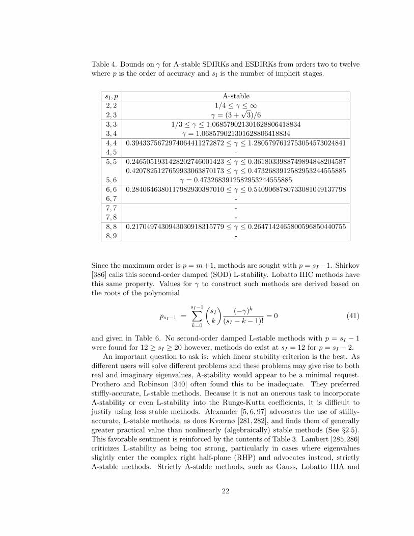
Table 4. Bounds on γ for A-stable SDIRKs and ESDIRKs from orders two to twelvewhere p is the order of accuracy and sI is the number of implicit stages.
sI, p A-stable
2, 2 1/4 ≤ γ ≤ ∞2, 3 γ = (3 +
√3)/6
3, 3 1/3 ≤ γ ≤ 1.0685790213016288064188343, 4 γ = 1.068579021301628806418834
4, 4 0.3943375672974064411272872 ≤ γ ≤ 1.28057976127530545730248414, 5 -
5, 5 0.2465051931428202746001423 ≤ γ ≤ 0.36180339887498948482045870.4207825127659933063870173 ≤ γ ≤ 0.4732683912582953244555885
5, 6 γ = 0.4732683912582953244555885
6, 6 0.2840646380117982930387010 ≤ γ ≤ 0.54090687807330810491377986, 7 -
7, 7 -7, 8 -
8, 8 0.2170497430943030918315779 ≤ γ ≤ 0.26471424658005968504407558, 9 -
Since the maximum order is p = m+1, methods are sought with p = sI−1. Shirkov[386] calls this second-order damped (SOD) L-stability. Lobatto IIIC methods havethis same property. Values for γ to construct such methods are derived based onthe roots of the polynomial
psI−1 =
sI−1∑k=0
(sIk
)(−γ)k
(sI − k − 1)!= 0 (41)
and given in Table 6. No second-order damped L-stable methods with p = sI − 1were found for 12 ≥ sI ≥ 20 however, methods do exist at sI = 12 for p = sI − 2.
An important question to ask is: which linear stability criterion is the best. Asdifferent users will solve different problems and these problems may give rise to bothreal and imaginary eigenvalues, A-stability would appear to be a minimal request.Prothero and Robinson [340] often found this to be inadequate. They preferredstiffly-accurate, L-stable methods. Because it is not an onerous task to incorporateA-stability or even L-stability into the Runge-Kutta coefficients, it is difficult tojustify using less stable methods. Alexander [5, 6, 97] advocates the use of stiffly-accurate, L-stable methods, as does Kværnø [281,282], and finds them of generallygreater practical value than nonlinearly (algebraically) stable methods (See §2.5).This favorable sentiment is reinforced by the contents of Table 3. Lambert [285,286]criticizes L-stability as being too strong, particularly in cases where eigenvaluesslightly enter the complex right half-plane (RHP) and advocates instead, strictlyA-stable methods. Strictly A-stable methods, such as Gauss, Lobatto IIIA and
22
Table 5. Bounds on γ for L-stable SDIRKs and ESDIRKs from orders two to twelvewhere p is the order of accuracy and sI is the number of implicit stages.
sI, p L-stable
2, 2 γ = (2±√
2)/2
3, 2 0.1804253064293985641345831 ≤ γ ≤ 2.18560009735504008262914003, 3 γ = 0.43586652150845899941601945
4, 3 0.2236478009341764510696898 ≤ γ ≤ 0.57281606248213485540800144, 4 γ = 0.5728160624821348554080014
5, 4 0.2479946362127474551679910 ≤ γ ≤ 0.67604239322628132887238635, 5 γ = 0.2780538411364523249315862
6, 5 0.1839146536751751632321436 ≤ γ ≤ 0.33414236706805043595403016, 6 γ = 0.3341423670680504359540301
7, 6 0.2040834517158857633717906 ≤ γ ≤ 0.37886489448532834402588537, 7 -
8, 7 0.1566585993970439483924506 ≤ γ ≤ 0.20293486084337767377793490.2051941719494007117460614 ≤ γ ≤ 0.2343731596055835579475589
8, 8 γ = 0.2343731596055835579475589
9, 8 0.1708919625574635309332223 ≤ γ ≤ 0.25942051048144255476694959, 9 -
10, 9 -10, 10 -
11, 10 0.1468989308591125260680428 ≤ γ ≤ 0.16579261009805605710961750.1937733662800920635754554 ≤ γ ≤ 0.1961524231108803003116274
11, 11 -
23
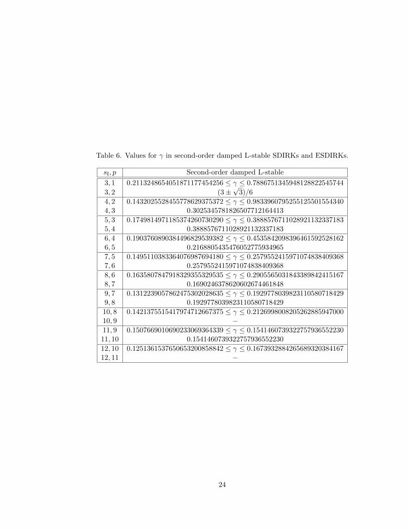
Table 6. Values for γ in second-order damped L-stable SDIRKs and ESDIRKs.
sI, p Second-order damped L-stable
3, 1 0.2113248654051871177454256 ≤ γ ≤ 0.7886751345948128822545744
3, 2 (3±√
3)/6
4, 2 0.1432025528455778629375372 ≤ γ ≤ 0.98339607952551255015543404, 3 0.3025345781826507712164413
5, 3 0.1749814971185374260730290 ≤ γ ≤ 0.38885767110289211323371835, 4 0.3888576711028921132337183
6, 4 0.1903760890384496829539382 ≤ γ ≤ 0.45358420983964615925281626, 5 0.2168805435476052775934965
7, 5 0.1495110383364076987694180 ≤ γ ≤ 0.25795524159710748384093687, 6 0.2579552415971074838409368
8, 6 0.1635807847918329355329535 ≤ γ ≤ 0.29055650318433898424151678, 7 0.1690246378620602674461848
9, 7 0.1312239057862475302028635 ≤ γ ≤ 0.19297780398231105807184299, 8 0.1929778039823110580718429
10, 8 0.1421375515417974712667375 ≤ γ ≤ 0.212699800820526288594700010, 9 −11, 9 0.1507669010690233069364339 ≤ γ ≤ 0.154146073932275793655223011, 10 0.1541460739322757936552230
12, 10 0.1251361537650653200858842 ≤ γ ≤ 0.167393288426568932038416712, 11 −
24
Lobatto IIIB methods, are those where E(y) = 0 and the stability boundary isexactly the imaginary axis. Both symmetric and symplectic DIRK-type methodsare also strictly A-stable.
Additional motivations may also be considered in the construction of desirablestability functions. In solving discretized PDEs using an approximately factorizedNewton iteration method, maximum step-sizes may not be governed by traditionalissues like A- or L-stability but rather by the spectral radius of the A-matrix, ρ(A).Van der Houwen and Sommeijer [215] construct A- and L-stable SDIRK methodsof orders two and three in two, three, or four stages, which minimize ρ(A). Atsecond-order, optimal methods have |P (iy)| = |Q(iy)|. Minimal ρ(A) is generallyachieved for all aii = γ. Another possible motivation related to space-time PDEs isto focus on the locations of the zeros of P (z) [424]. The goal might be to determinethe location of scaled eigenvalues zi = λi(∆t), which correspond to poorly resolvedspatial information, and to set P (zi) = 0. This approach has been done for explicitRunge-Kutta (ERK) methods and requires s� p to be able to exert any meaningfulcontrol.
Three further stability concepts to be mentioned are S-, D- and AS-stability. S-and strong S-stability were introduced by Prothero and Robinson [340] to extendthe concepts of A- and L-stability to the nonhomogeneous test equation y′(t) =g′(t) + λ (y(t)− g(t)). One may also speak of S(α)-stable methods. Alexander [5]and others [92, 209, 280] derive several strongly S-stable SDIRKs; however, Zhao etal. [465] claim that the concept of S-stability is fundamentally flawed and that noconsistent, well-defined Runge-Kutta method is S-stable. Alexander states thatan A-stable DIRK-type method with positive aii and invertible A-matrix is S-stable if and only if |R(−∞)| < 1. An S-stable method is strongly S-stable ifand only if it is stiffly-accurate. Decomposition- or D-stability [129] is not a tradi-tional stability measure in that it is not concerned with the propagation of errors.It is concerned with the boundedness of stiff, linear, nonautonomous problems.Hairer [183] states that D-stability requires that the eigenvalues of aij lie in thecomplex RHP (<(λaij ) > 0). If aij is singular (EDIRK, ESDIRK, or QESDIRKmethods), then only reducible or confluent methods can be D-stable. If a Runge-Kutta method is irreducible and deg Q(z) = s, then A-stability implies D-stability.AS-stability [57, 77, 123] is the linear analog of the more familiar nonlinear BS-stability concept and plays an essential role in the convergence analysis of stiff semi-linear problems with constant coefficients. A method is called AS-stable if (I− zA)is nonsingular for all z in the complex LHP and ||zbT (I − zA)−1|| is uniformlybounded in an inner product norm within the complex LHP. Stability analysis ofnonautonomous linear problems focuses on AN-stability using the K-function
K(Z) = 1 + bTZ(I−AZ)−1e =det[I− (A− e⊗ bT )Z
]det [I−AZ]
, (42)
where Z = diag{z1, z2, · · · , zs} and which, surprisingly, is more properly investigatedwithin the purview of nonlinear stability. Following Burrage and Butcher [53], theK-function for Runge-Kutta methods is given as
K(Z) = 1 + eTBZ [I−AZ]−1 e, (43)
25
where B = diag(bT). A Runge-Kutta is AN-stable if |K(Z)| ≤ 1, <(zi) ≤ 0 for all
zi, i = 1, 2, . . . , s such that zi = zj whenever ci = cj . Defining Kint = (I−AZ)−1 eand e = (I−AZ)Kint, then
K(Z) = 1 + eTBZKint, K(Z) = 1 + KTintZBTe (44)
with the superscript denoting the complex conjugate. Therefore, since (BTe)(eTB) =BBT ,
|K(Z)| = K(Z)K(Z) = 1 + eTBZKint + KTintZBTe + KTintZBBTZKint (45)
= 1 + KTint
(BZ + ZBT
)Kint
− KTintZk(BTA + ATB−BBT
)ZKint, (46)
where expressions for e and its transpose were used. Defining the symmetric alge-braic stability matrix as
M = BTA + ATB−BBT , Mij = biaij + bjaji − bibj , i, j = 1, 2, . . . , s, (47)
then
|K(Z)| − 1 = 2<(KTintBZKint
)− KTintZMZKint
= 2
(s∑i=1
bi< (zi) |K(i)int|
2
)−
s∑i,j=1
K(i)intziMijzjK
(j)int , (48)
where K(i)int are the components of the vector Kint, which will be seen below to be the
nonautonomous internal stability function. If the Runge-Kutta method is AN-stablethen, |K(Z)| ≤ 1 or
|K(Z)| − 1 = 2
(s∑i=1
bi< (zi) |K(i)int|
2
)−
s∑i,j=1
K(i)intziMijzjK
(j)int ≤ 0 (49)
for all zi such that zi = zj whenever ci = cj where <(zi) ≤ 0. It will be seen in thenext section that this result has much in common with algebraic stability exceptwhen the method is confluent.
2.5 Nonlinear Stability
Maximum norm and inner product norm contractivity on nonlinear problems aswell as nonlinear stability [51–53,89,122,125,126,129,192,193,251,252,266,267,287,300, 312, 313, 362, 456, 469] may be considered for DIRK-type methods. Stabilityand contractivity are related, but contractivity is generally a stronger requirement[125,126,268,409,412]. For ODE systems where the difference between two solutions
satisfies ||U(t + ∆t) − U(t + ∆t)|| ≤ ||U(t) − U(t)|| in some norm (a dissipativitycondition) for ∆t > 0, one might reasonably demand of the numerical method
that ||U (n) − U (n)|| ≤ αnβ||U (0) − U (0)|| in that same norm where α and β denotepositive real constants and n ≥ 1 denotes the number of time steps [412]. In the
26
case where β = 0 and α = 1, one has contractivity. If β = 0 but α is of moderatesize, one has strong stability, but if both α and β are of moderate size then onehas only weak stability. Nonlinear stability of implicit Runge-Kutta methods isgenerally characterized in terms of algebraic-, B-, BN-, or AN-stability and requiresa dissipativity condition on the underlying ODEs. Each of these measures impliesA-stability. The first three also imply unconditional contractivity (unlimited stepsize) in an inner product norm, rF2 =∞ where F denotes a nonlinear RHS, for bothconfluent and nonconfluent Runge-Kutta methods [270]. For nonconfluent methods,each of these four concepts is equivalent. For confluent methods, B- and BN-stabilityare equivalent to algebraic-stability but AN-stability is not [129, 193, 300]. It issufficient for the present purposes to focus simply on algebraic-stability. In the innerproduct norm case, one constructs the matricesM and B = diag(b) or b = Be using
the algebraic stability matrix asM = B−1/2MB−1/2 where the former expression isused only when b > 0. An analogous construction may be made for the embeddedmethod by replacing b with b. The most general algebraic stability is (k, l)-algebraicstability [52,251] where the more common algebraic-stability is retrieved with k = 1,l = 0. Algebraic-stability [410] of irreducible methods requires that aii, bi > 0 andM ≥ O. Consequently, DIRKs, SDIRKs and QSDIRKs may be algebraically stablebut EDIRKs, ESDIRKs and QESDIRKs may not. The maximum order of accuracyfor an algebraically stable DIRK-type scheme is four [181]. Burrage and Butcher [53]and Crouzeix [122] were the first to characterize the nonlinear stability of DIRK-typemethods by showing that two methods, a two-stage, third-order (SDIRK-NCS23)and a three-stage, fourth-order (SDIRK-NC34) SDIRK, due to Nørsett [308] andCrouzeix [120] (and Scherer [357] on SDIRK-NCS23), were algebraically stable
γ γ 01− γ 1− 2γ γ
12
12
γ γ 0 012
12 − γ γ 0
1− γ 2γ 1− 4γ γ1
6(1−2γ)22(1−6γ+6γ2)
3(2γ−1)21
6(1−2γ)2
(50)
where γ = 3+√
36 ≈ 0.7887 and R(−∞) = 1.0 for the two-stage method, and
γ =3+2√
3 cos( π18)6 ≈ 1.069 and R(−∞) = −0.732 for the three-stage method. The
two-stage method also appears in a paper by Makinson [296], but in the contextof Rosenbrock methods. Burrage and Butcher [53] present an interesting SDIRKmethod
γ γ 0 0 · · · 0γ + b1 b1 γ 0 · · · 0
γ + b1 + b2 b1 b2 γ. . .
......
......
. . .. . . 0
γ +∑s−1i=1 bi b1 b2 · · · bs−1 γ
b1 b2 · · · bs−1 bs
(51)
where the resulting algebraic-stability matrix is diagonal with entries Mii = bi(2γ−bi) and i = 1, 2, · · · , s. We remark that the form of this Butcher array is reminiscentof the van der Houwen approach to memory storage reduction [256]. Burrage [51]presents second-, third-, and fourth-order algebraically stable SDIRK methods upto four stages. At two stages, SDIRK-NCS23 given previously (with a different γ)is algebraically stable and second-order accurate for γ ≥ 1/4, γ 6= 1/2 and is third-
27
order accurate for γ = 3+√
36 . At three and four stages, Burrage gives complete class
of nonconfluent algebraically stable SDIRKs of orders three and four are given. Todesign these algebraically stable methods, Burrage defines a symmetric matrix R =VTMV by using the algebraic-stability matrix and the van der Monde matrix, Vij =
cj−1i , i, j = 1, 2, · · · , s. It may be shown that all elements of Rij vanish for i+j ≤ p,
where p is the classical order of the method. Assuming a nonconfluent method, theirreducible DIRK-type method is algebraically stable if R ≥ O and b > 0. Nørsettand Thomsen [312] derive an algebraically stable, three-stage SDIRK, with an A-stable embedded method of order two. Cameron [89] derives two algebraically andL-stable, four-stage, third-order DIRKs along with an algebraically stable, three-stage SDIRK method.
Cooper [115] offers a less restrictive form of nonlinear stability called weak B-stability. It requires the existence of a symmetric matrix D such that b ≥ 0 andDA + ATD − bTb ≥ O, with De = b and dij ≤ 0 for i 6= j. He shows that thetwo-stage, second-order SDIRK method is both B-stable and weakly B-stable forγ ≥ 1/4 but is weakly B-stable for 0 ≤ b2 ≤ 1/2 and B-stable for only b2 = 1/2.Weak stability is closely related to what Spijker [411] calls weak contractivity. Hesimultaneously generalizes algebraic-stability and weak B-stability by consideringa modified dissipativity condition to study contractivity and weak contractivity.Rather than weakening algebraic-stability, passive and lossless Runge-Kutta meth-ods require more than algebraic-stability [158, 159, 319]. Passive methods requirethat all elements of b be identical along with algebraic-stability. Lossless methodsrequire the method to be both passive and symplectic.
An important question is whether algebraic-stability matters in a practical sense.Hairer [184] constructs a one-parameter family of A-stable, three-stage, fourth-order, fully implicit Runge-Kutta methods by using assumptions C(1), D(1), ci ={0, 1/2, 1} and bi = {1/6, 4/6, 1/6}. For a specific value of the parameter, themethod becomes algebraically stable. The method was tested on Kreiss’s prob-lem [129] which, in the limit of infinite stiffness, transforms from an ODE to anindex-2 DAE. Behavior of the methods was best for choices of the parameter thatnearly, but not exactly, corresponded to algebraic-stability. Scheme efficiency wasrelatively insensitive to the parameter at coarse tolerances but became stronglydependent on it at strict tolerances. Contractivity was a strong function of theparameter at all tolerances. For all values of the adjustable parameter, all internalstages were completely damped for z → −∞. It was not clear how changing thevalue of the adjustable parameter affected the satisfaction of index-2 DAE orderconditions for the method. In another effort to assess the practical value of alge-braically stable methods, Verwer [436] considers whether the stability property ispreserved during implementation with a Newton-type solver. If users are willing toreevaluate the Jacobian at each stage, algebraic-stability is preserved; otherwise, itis generally not preserved. Spijker [412] asks whether methods exist that possessstrong or weak stability but not contractivity (algebraic-stability) on (1), subjectto a dissipativity condition. Kraaijevanger and Spijker [270] construct the DIRK
28
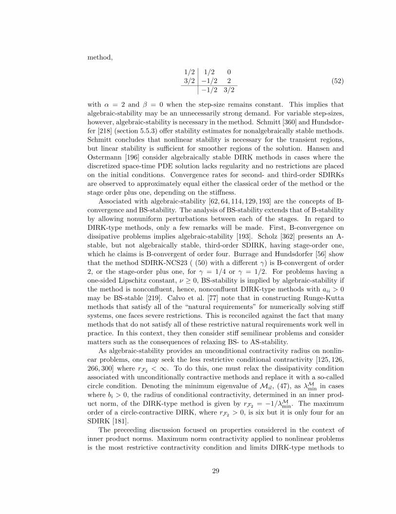
method,
1/2 1/2 03/2 −1/2 2
−1/2 3/2
(52)
with α = 2 and β = 0 when the step-size remains constant. This implies thatalgebraic-stability may be an unnecessarily strong demand. For variable step-sizes,however, algebraic-stability is necessary in the method. Schmitt [360] and Hundsdor-fer [218] (section 5.5.3) offer stability estimates for nonalgebraically stable methods.Schmitt concludes that nonlinear stability is necessary for the transient regions,but linear stability is sufficient for smoother regions of the solution. Hansen andOstermann [196] consider algebraically stable DIRK methods in cases where thediscretized space-time PDE solution lacks regularity and no restrictions are placedon the initial conditions. Convergence rates for second- and third-order SDIRKsare observed to approximately equal either the classical order of the method or thestage order plus one, depending on the stiffness.
Associated with algebraic-stability [62, 64, 114, 129, 193] are the concepts of B-convergence and BS-stability. The analysis of BS-stability extends that of B-stabilityby allowing nonuniform perturbations between each of the stages. In regard toDIRK-type methods, only a few remarks will be made. First, B-convergence ondissipative problems implies algebraic-stability [193]. Scholz [362] presents an A-stable, but not algebraically stable, third-order SDIRK, having stage-order one,which he claims is B-convergent of order four. Burrage and Hundsdorfer [56] showthat the method SDIRK-NCS23 ( (50) with a different γ) is B-convergent of order2, or the stage-order plus one, for γ = 1/4 or γ = 1/2. For problems having aone-sided Lipschitz constant, ν ≥ 0, BS-stability is implied by algebraic-stability ifthe method is nonconfluent, hence, nonconfluent DIRK-type methods with aii > 0may be BS-stable [219]. Calvo et al. [77] note that in constructing Runge-Kuttamethods that satisfy all of the “natural requirements” for numerically solving stiffsystems, one faces severe restrictions. This is reconciled against the fact that manymethods that do not satisfy all of these restrictive natural requirements work well inpractice. In this context, they then consider stiff semilinear problems and considermatters such as the consequences of relaxing BS- to AS-stability.
As algebraic-stability provides an unconditional contractivity radius on nonlin-ear problems, one may seek the less restrictive conditional contractivity [125, 126,266, 300] where rF2 < ∞. To do this, one must relax the dissipativity conditionassociated with unconditionally contractive methods and replace it with a so-calledcircle condition. Denoting the minimum eigenvalue of Mil, (47), as λMmin in caseswhere bi > 0, the radius of conditional contractivity, determined in an inner prod-uct norm, of the DIRK-type method is given by rF2 = −1/λMmin. The maximumorder of a circle-contractive DIRK, where rF2 > 0, is six but it is only four for anSDIRK [181].
The preceeding discussion focused on properties considered in the context ofinner product norms. Maximum norm contractivity applied to nonlinear problemsis the most restrictive contractivity condition and limits DIRK-type methods to
29
first-order accuracy if unconditional contractivity, rF∞= ∞, is desired [266]. Asmentioned earlier, this order barrier does not change if the nonlinear problem isreplaced with a linear one, where rL∞= ∞. Relaxing unconditional to conditionalcontractivity so that the maximum-norm conditional contractivity radius, rF∞> 0rather than rF∞= ∞, one requires that beyond aij , bi > 0, that (I − ξA) is non-singular and R(ξ) ≥ 0, A(ξ) = A(I − ξA)−1 ≥ 0, B(ξ) = bT(I − ξA)−1 ≥ 0and E(ξ) = (I − ξA)−1e ≥ 0, where rF∞ is the smallest value of ξ for which allcomponents of R(ξ), A(ξ), B(ξ) and E(ξ) are non-negative. Kraaijevanger [266]constructs a fifth-order EDIRK that is neither algebraically stable nor A-stable yethas nonvanishing contractivity radii of rF∞= 0.5906 and rF2 = 2.489. Ferracinaand Spijker [148, 149] give the maximally contractive SDIRK in two stages, (78),with rF∞= 2. They also show that any method which is optimal in the sense thatrF∞ is maximized also is optimal in the sense of maximizing the step-size for a totalvariation diminishing (TVD) Runge-Kutta process. In a later paper, Ferracina andSpijker [150] establish rF∞for SDIRKs at orders one through four and stage numbersfrom one to eight. Duraisamy et al. [134] also consider TVD SDIRKs. Ketcheson etal. [257] include fully implicit Runge-Kutta methods as well as DIRK-methods toorder six while Gottlieb et al. [177, 178] also include multistep methods. Extensionof BS-stability bounds to the max norm is given by Kraaijevanger [266]. Positivityof aij and bi in a DIRK are also useful preserving the monotonicity behavior oflinear differential equations decribing dynamical systems during numerical integra-tion [259]. Hundsdorfer and Spijker [221] relate the results of Kraaijevanger [266]to the topic of boundedness including the total variation bounded (TVB) property.Step-size restrictions dictated by rF∞are found to also apply if a TVB property isdesired except for a very special class of irreducible RK-methods. This special classhas a zero row in its A-matrix and another row equal to b.
2.6 Internal Stability
Beyond traditional stepwise stability, it may be useful to control the stability as-sociated with each stage in addition to each step. This is particularly true forlarge scaled eigenvalues, z, associated with stiff problems [255,436]. IMEX additiveRunge-Kutta methods are especially sensitive to the internal stability of the implicitmethod [255]. Kurdi [278] appears to have been the first to consider the internalstability of DIRK-type methods. To determine the vector of internal stabilities ofRunge-Kutta methods, one evaluates
Rint(z) = (I− zA)−1e = {R(1)int (z), R
(2)int (z), · · · , R(s)
int(z)}T
=
{P
(1)int (z)
Q(1)int(z)
,P
(2)int (z)
Q(2)int(z)
, · · · ,P
(s)int (z)
Q(s)int(z)
}T. (53)
The primary concern will be the value of R(i)int(−∞). For DIRK-type methods,
P(i)int (z) is generally a polynomial of degree i− 1 in z because a stage-wise version of
the stiffly-accurate assumption holds while Q(i)int(z) is generally of degree i. Conse-
quently, DIRKs with aii 6= 0 and SDIRKs have R(i)int(−∞) = 0. EDIRKs, ESDIRKs
30
and QESDIRKs with Q(i)int(z) reduced to degree i− 1 because a11 = 0, then they do
not generally satisfy R(i)int(−∞) = 0. If EDIRK, ESDIRK and QESDIRK methods
satisfy C(1), then R(1)int (−∞) = 1. If the EDIRK, ESDIRK, or QESDIRK satisfies
C(2), then R(2)int (−∞) = −1. One may also consider the E-polynomial, (40), at
internal stages to determine stage-wise I-stability by using
E(i)int(y) = Q
(i)int(iy)Q
(i)int(−iy)− P (i)
int (iy)P(i)int (−iy). (54)
To assess the internal AN-stability with regard to nonautonomous linear equations,one may consider evaluating the Runge-Kutta K-function [266] at internal stages
Kint(Z) = (I−AZ)−1e = {K(1)int (Z),K
(2)int (Z), · · · ,K(s)
int (Z)}T . (55)
One could also consider a stage-wise analog to the algebraic-stability matrix. Fol-lowing section 4.2 of Dekker and Verwer [129], one may derive the following step
||U [n+1]||2 − ||U [n]||2 = 2(∆t)s∑j=1
bj < Uj , Fj >
− (∆t)2s∑
j,k=1
(bjajk + bkakj − bjbk) < Fj , Fk > (56)
and stage
||Ui||2 − ||U [n]||2 = 2(∆t)
s∑j=1
aij < Uj , Fj >
− (∆t)2s∑
j,k=1
(aijajk + aikakj − aijaik) < Fj , Fk > (57)
relations where
M(i)jk = aijajk + aikakj − aijaik (58)
is the internal algebraic-stability matrix for stage i. Hence, for internal algebraicstability on stage i of an irreducible method, it is necessary that M(i) ≥ O and thataij ≥ 0. This matrix has been considered by Burrage and Butcher [53] but it doesnot appear to have ever been considered in this context.
Internal stability influences on methods have been studied in several differentcontexts. Calvo et al. [76] consider, in part, the effect of internal stability on theconvergence of IRK methods applied to stiff, nonlinear, dissipative ODEs. Gonzalez-Pinto et al. [173–175] factor internal stability into the design of starting algorithmsfor implicit Runge-Kutta methods. It is for the preservation of internal stabilitythat it is unwise to use aii = 0 on any stage but the first.
Several additional internal stability concepts include ASI-stability [57,77,123] forlinear problems and BSI-stability [64,129,193] for nonlinear problems. A method is
31
ASI-stable if the matrix (I − zA) is nonsingular for all z in the complex LHP andits inverse is uniformly bounded in the complex LHP in an inner product norm. Ifthere exists a positive definite, diagonal matrix D, such that DA + ATD is positivedefinite, then the Runge-Kutta method is BSI-stable [128]. This requirement isonly achievable for DIRK-type methods if aii > 0 [219]. Kraaijevanger [266] givesBSI-stability bounds valid in all norms, not just an inner product norm. InternalS-stability has been considered by Verwer [435] and internal D-stability is discussedby Dekker and Verwer [129].
2.7 Dense Output
On occasion, it may be necessary to determine the value of the integration vector attime locations not coincident with a time step (t[n]) or stage location (t[n] + ci∆t).Dense output [190, 332] provides a mechanism that allows high-order interpolationof the integration variables at any point, t[n] + θ∆t, inside the current integrationstep where 0 ≤ θ ≤ 1 by using
U(t[n] + θ∆t) ∼= U [n] + (∆t)s∑i=1
b∗i (θ)Fi, b∗i (θ) =
p∗∑j=1
b∗ijθj , b∗i (θ = 1) = bi, (59)
where p∗ is the lowest order of the interpolant on the interval 0 ≤ θ ≤ 1. Byconstruction, b∗i (θ = 0) = 0. Order conditions at order m and the stability functionR∗(z, θ) for the dense-output method are given by [35]
τ∗(m)j =
1
σ
s∑i
b∗i (θ)Φ(m)i,j −
αθm
m!, R∗(z, θ) =
Det[I− zA + ze⊗ b∗T (θ)
]Det [I− zA]
. (60)
Setting m = p and θ = 1 retrieves the standard Runge-Kutta order conditions.As with the main and embedded formulas, one may write terms like A∗(p
∗+1) =A∗(p
∗+1)(θ) to access the truncation error of the dense output method. Relativelyfew DIRK-type methods appearing in the literature include dense output [89, 193,255,280,382–384,426]. As with embedded methods, dense output methods could beenhanced by using a two-step procedure [176].
2.8 Conservation, Symplecticity and Symmetry
All consistent DIRK, SDIRK and ESDIRK methods conserve linear first integrals[188]. To conserve quadratic and cubic first integrals, one focuses on the symmetricmatrices
Mij = biaij + bjaji − bibj (61)
Mijk = biaijajk + bjajkaki + bkakiaij
− (bibjaik + bjbkaji + bkbiakj) + bibjbk (62)
with magnitudes that may be defined as ||Mij || =(∑s
i,j=1MijMij
)1/2and ||Mijk|| =(∑s
i,j,k=1 MijkMijk
)1/2. Methods having Mij = 0 conserve certain quadratic first
32
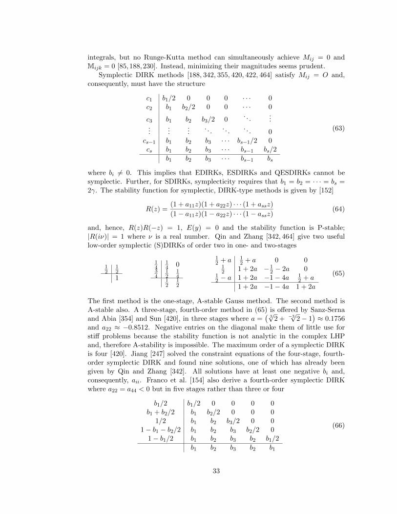
integrals, but no Runge-Kutta method can simultaneously achieve Mij = 0 andMijk = 0 [85,188,230]. Instead, minimizing their magnitudes seems prudent.
Symplectic DIRK methods [188, 342, 355, 420, 422, 464] satisfy Mij = O and,consequently, must have the structure
c1 b1/2 0 0 0 · · · 0c2 b1 b2/2 0 0 · · · 0
c3 b1 b2 b3/2 0. . .
......
......
. . .. . .
. . . 0cs−1 b1 b2 b3 · · · bs−1/2 0cs b1 b2 b3 · · · bs−1 bs/2
b1 b2 b3 · · · bs−1 bs
(63)
where bi 6= 0. This implies that EDIRKs, ESDIRKs and QESDIRKs cannot besymplectic. Further, for SDIRKs, symplecticity requires that b1 = b2 = · · · = bs =2γ. The stability function for symplectic, DIRK-type methods is given by [152]
R(z) =(1 + a11z)(1 + a22z) · · · (1 + assz)
(1− a11z)(1− a22z) · · · (1− assz)(64)
and, hence, R(z)R(−z) = 1, E(y) = 0 and the stability function is P-stable;|R(iν)| = 1 where ν is a real number. Qin and Zhang [342, 464] give two usefullow-order symplectic (S)DIRKs of order two in one- and two-stages
12
12
1
14
14 0
34
12
14
12
12
12 + a 1
2 + a 0 012 1 + 2a −1
2 − 2a 012 − a 1 + 2a −1− 4a 1
2 + a
1 + 2a −1− 4a 1 + 2a
(65)
The first method is the one-stage, A-stable Gauss method. The second method isA-stable also. A three-stage, fourth-order method in (65) is offered by Sanz-Sernaand Abia [354] and Sun [420], in three stages where a =
(3√
2 + −3√
2− 1)≈ 0.1756
and a22 ≈ −0.8512. Negative entries on the diagonal make them of little use forstiff problems because the stability function is not analytic in the complex LHPand, therefore A-stability is impossible. The maximum order of a symplectic DIRKis four [420]. Jiang [247] solved the constraint equations of the four-stage, fourth-order symplectic DIRK and found nine solutions, one of which has already beengiven by Qin and Zhang [342]. All solutions have at least one negative bi and,consequently, aii. Franco et al. [154] also derive a fourth-order symplectic DIRKwhere a22 = a44 < 0 but in five stages rather than three or four
b1/2 b1/2 0 0 0 0b1 + b2/2 b1 b2/2 0 0 0
1/2 b1 b2 b3/2 0 01− b1 − b2/2 b1 b2 b3 b2/2 0
1− b1/2 b1 b2 b3 b2 b1/2
b1 b2 b3 b2 b1
(66)
33
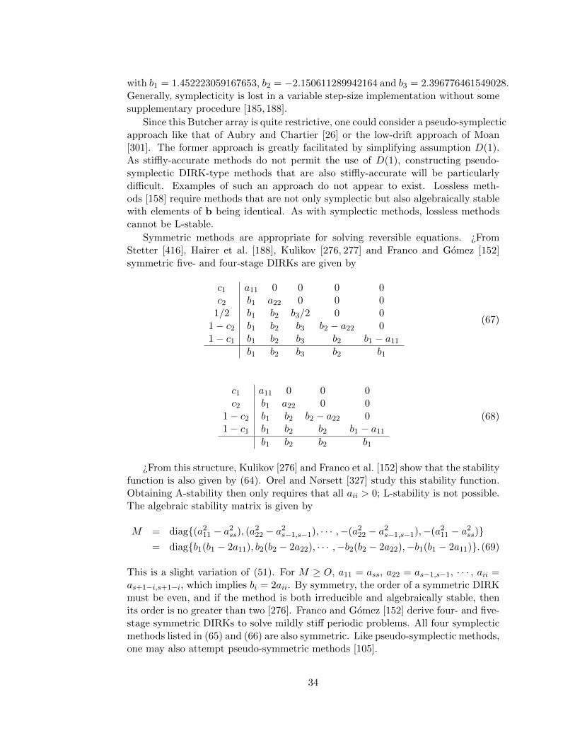
with b1 = 1.452223059167653, b2 = −2.150611289942164 and b3 = 2.396776461549028.Generally, symplecticity is lost in a variable step-size implementation without somesupplementary procedure [185,188].
Since this Butcher array is quite restrictive, one could consider a pseudo-symplecticapproach like that of Aubry and Chartier [26] or the low-drift approach of Moan[301]. The former approach is greatly facilitated by simplifying assumption D(1).As stiffly-accurate methods do not permit the use of D(1), constructing pseudo-symplectic DIRK-type methods that are also stiffly-accurate will be particularlydifficult. Examples of such an approach do not appear to exist. Lossless meth-ods [158] require methods that are not only symplectic but also algebraically stablewith elements of b being identical. As with symplectic methods, lossless methodscannot be L-stable.
Symmetric methods are appropriate for solving reversible equations. ¿FromStetter [416], Hairer et al. [188], Kulikov [276, 277] and Franco and Gomez [152]symmetric five- and four-stage DIRKs are given by
c1 a11 0 0 0 0c2 b1 a22 0 0 0
1/2 b1 b2 b3/2 0 01− c2 b1 b2 b3 b2 − a22 01− c1 b1 b2 b3 b2 b1 − a11
b1 b2 b3 b2 b1
(67)
c1 a11 0 0 0c2 b1 a22 0 0
1− c2 b1 b2 b2 − a22 01− c1 b1 b2 b2 b1 − a11
b1 b2 b2 b1
(68)
¿From this structure, Kulikov [276] and Franco et al. [152] show that the stabilityfunction is also given by (64). Orel and Nørsett [327] study this stability function.Obtaining A-stability then only requires that all aii > 0; L-stability is not possible.The algebraic stability matrix is given by
M = diag{(a211 − a2
ss), (a222 − a2
s−1,s−1), · · · ,−(a222 − a2
s−1,s−1),−(a211 − a2
ss)}= diag{b1(b1 − 2a11), b2(b2 − 2a22), · · · ,−b2(b2 − 2a22),−b1(b1 − 2a11)}. (69)
This is a slight variation of (51). For M ≥ O, a11 = ass, a22 = as−1,s−1, · · · , aii =as+1−i,s+1−i, which implies bi = 2aii. By symmetry, the order of a symmetric DIRKmust be even, and if the method is both irreducible and algebraically stable, thenits order is no greater than two [276]. Franco and Gomez [152] derive four- and five-stage symmetric DIRKs to solve mildly stiff periodic problems. All four symplecticmethods listed in (65) and (66) are also symmetric. Like pseudo-symplectic methods,one may also attempt pseudo-symmetric methods [105].
34
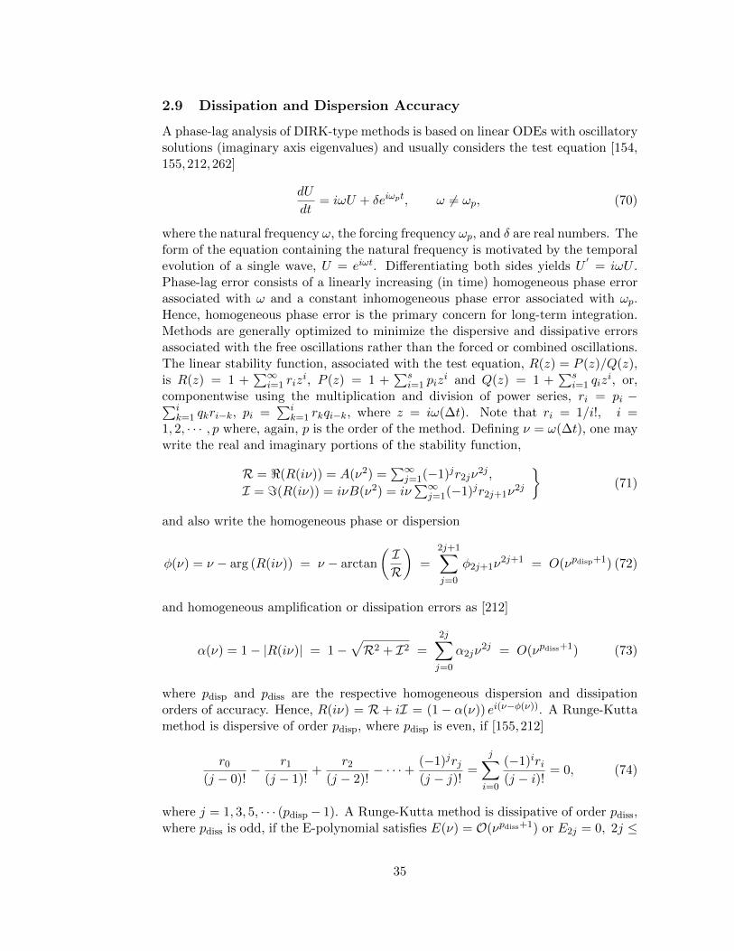
2.9 Dissipation and Dispersion Accuracy
A phase-lag analysis of DIRK-type methods is based on linear ODEs with oscillatorysolutions (imaginary axis eigenvalues) and usually considers the test equation [154,155,212,262]
dU
dt= iωU + δeiωpt, ω 6= ωp, (70)
where the natural frequency ω, the forcing frequency ωp, and δ are real numbers. Theform of the equation containing the natural frequency is motivated by the temporalevolution of a single wave, U = eiωt. Differentiating both sides yields U
′= iωU .
Phase-lag error consists of a linearly increasing (in time) homogeneous phase errorassociated with ω and a constant inhomogeneous phase error associated with ωp.Hence, homogeneous phase error is the primary concern for long-term integration.Methods are generally optimized to minimize the dispersive and dissipative errorsassociated with the free oscillations rather than the forced or combined oscillations.The linear stability function, associated with the test equation, R(z) = P (z)/Q(z),is R(z) = 1 +
∑∞i=1 riz
i, P (z) = 1 +∑s
i=1 pizi and Q(z) = 1 +
∑si=1 qiz
i, or,componentwise using the multiplication and division of power series, ri = pi −∑i
k=1 qkri−k, pi =∑i
k=1 rkqi−k, where z = iω(∆t). Note that ri = 1/i!, i =1, 2, · · · , p where, again, p is the order of the method. Defining ν = ω(∆t), one maywrite the real and imaginary portions of the stability function,
R = <(R(iν)) = A(ν2) =∑∞
j=1(−1)jr2jν2j ,
I = =(R(iν)) = iνB(ν2) = iν∑∞
j=1(−1)jr2j+1ν2j
}(71)
and also write the homogeneous phase or dispersion
φ(ν) = ν − arg (R(iν)) = ν − arctan
(IR
)=
2j+1∑j=0
φ2j+1ν2j+1 = O(νpdisp+1) (72)
and homogeneous amplification or dissipation errors as [212]
α(ν) = 1− |R(iν)| = 1−√R2 + I2 =
2j∑j=0
α2jν2j = O(νpdiss+1) (73)
where pdisp and pdiss are the respective homogeneous dispersion and dissipationorders of accuracy. Hence, R(iν) = R+ iI = (1− α(ν)) ei(ν−φ(ν)). A Runge-Kuttamethod is dispersive of order pdisp, where pdisp is even, if [155,212]
r0
(j − 0)!− r1
(j − 1)!+
r2
(j − 2)!− · · ·+ (−1)jrj
(j − j)!=
j∑i=0
(−1)iri(j − i)!
= 0, (74)
where j = 1, 3, 5, · · · (pdisp− 1). A Runge-Kutta method is dissipative of order pdiss,where pdiss is odd, if the E-polynomial satisfies E(ν) = O(νpdiss+1) or E2j = 0, 2j ≤
35
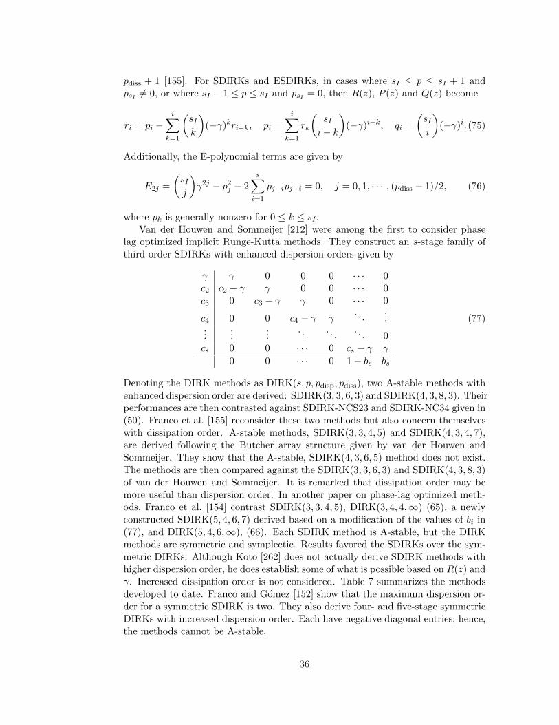
pdiss + 1 [155]. For SDIRKs and ESDIRKs, in cases where sI ≤ p ≤ sI + 1 andpsI 6= 0, or where sI − 1 ≤ p ≤ sI and psI = 0, then R(z), P (z) and Q(z) become
ri = pi −i∑
k=1
(sIk
)(−γ)kri−k, pi =
i∑k=1
rk
(sIi− k
)(−γ)i−k, qi =
(sIi
)(−γ)i. (75)
Additionally, the E-polynomial terms are given by
E2j =
(sIj
)γ2j − p2
j − 2s∑i=1
pj−ipj+i = 0, j = 0, 1, · · · , (pdiss − 1)/2, (76)
where pk is generally nonzero for 0 ≤ k ≤ sI .Van der Houwen and Sommeijer [212] were among the first to consider phase
lag optimized implicit Runge-Kutta methods. They construct an s-stage family ofthird-order SDIRKs with enhanced dispersion orders given by
γ γ 0 0 0 · · · 0c2 c2 − γ γ 0 0 · · · 0c3 0 c3 − γ γ 0 · · · 0
c4 0 0 c4 − γ γ. . .
......
......
. . .. . .
. . . 0cs 0 0 · · · 0 cs − γ γ
0 0 · · · 0 1− bs bs
(77)
Denoting the DIRK methods as DIRK(s, p, pdisp, pdiss), two A-stable methods withenhanced dispersion order are derived: SDIRK(3, 3, 6, 3) and SDIRK(4, 3, 8, 3). Theirperformances are then contrasted against SDIRK-NCS23 and SDIRK-NC34 given in(50). Franco et al. [155] reconsider these two methods but also concern themselveswith dissipation order. A-stable methods, SDIRK(3, 3, 4, 5) and SDIRK(4, 3, 4, 7),are derived following the Butcher array structure given by van der Houwen andSommeijer. They show that the A-stable, SDIRK(4, 3, 6, 5) method does not exist.The methods are then compared against the SDIRK(3, 3, 6, 3) and SDIRK(4, 3, 8, 3)of van der Houwen and Sommeijer. It is remarked that dissipation order may bemore useful than dispersion order. In another paper on phase-lag optimized meth-ods, Franco et al. [154] contrast SDIRK(3, 3, 4, 5), DIRK(3, 4, 4,∞) (65), a newlyconstructed SDIRK(5, 4, 6, 7) derived based on a modification of the values of bi in(77), and DIRK(5, 4, 6,∞), (66). Each SDIRK method is A-stable, but the DIRKmethods are symmetric and symplectic. Results favored the SDIRKs over the sym-metric DIRKs. Although Koto [262] does not actually derive SDIRK methods withhigher dispersion order, he does establish some of what is possible based on R(z) andγ. Increased dissipation order is not considered. Table 7 summarizes the methodsdeveloped to date. Franco and Gomez [152] show that the maximum dispersion or-der for a symmetric SDIRK is two. They also derive four- and five-stage symmetricDIRKs with increased dispersion order. Each have negative diagonal entries; hence,the methods cannot be A-stable.
36
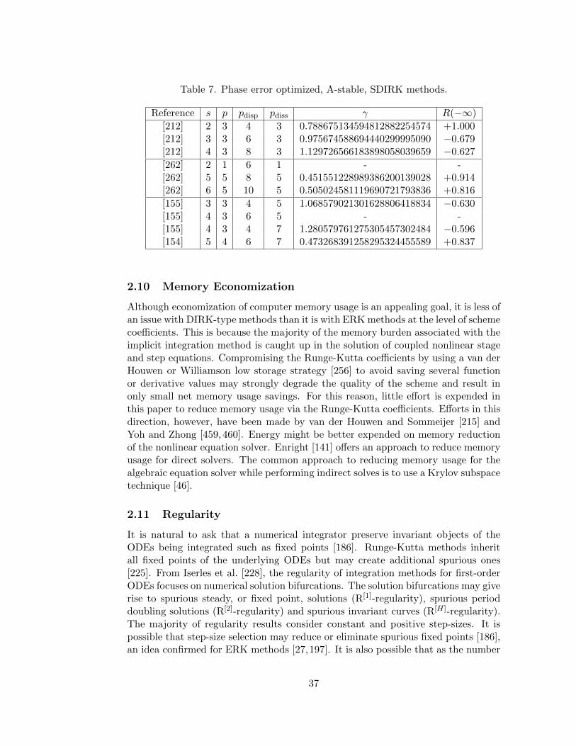
Table 7. Phase error optimized, A-stable, SDIRK methods.
Reference s p pdisp pdiss γ R(−∞)
[212] 2 3 4 3 0.788675134594812882254574 +1.000[212] 3 3 6 3 0.975674588694440299995090 −0.679[212] 4 3 8 3 1.129726566183898058039659 −0.627
[262] 2 1 6 1 - -[262] 5 5 8 5 0.451551228989386200139028 +0.914[262] 6 5 10 5 0.505024581119690721793836 +0.816
[155] 3 3 4 5 1.068579021301628806418834 −0.630[155] 4 3 6 5 - -[155] 4 3 4 7 1.280579761275305457302484 −0.596[154] 5 4 6 7 0.473268391258295324455589 +0.837
2.10 Memory Economization
Although economization of computer memory usage is an appealing goal, it is less ofan issue with DIRK-type methods than it is with ERK methods at the level of schemecoefficients. This is because the majority of the memory burden associated with theimplicit integration method is caught up in the solution of coupled nonlinear stageand step equations. Compromising the Runge-Kutta coefficients by using a van derHouwen or Williamson low storage strategy [256] to avoid saving several functionor derivative values may strongly degrade the quality of the scheme and result inonly small net memory usage savings. For this reason, little effort is expended inthis paper to reduce memory usage via the Runge-Kutta coefficients. Efforts in thisdirection, however, have been made by van der Houwen and Sommeijer [215] andYoh and Zhong [459, 460]. Energy might be better expended on memory reductionof the nonlinear equation solver. Enright [141] offers an approach to reduce memoryusage for direct solvers. The common approach to reducing memory usage for thealgebraic equation solver while performing indirect solves is to use a Krylov subspacetechnique [46].
2.11 Regularity
It is natural to ask that a numerical integrator preserve invariant objects of theODEs being integrated such as fixed points [186]. Runge-Kutta methods inheritall fixed points of the underlying ODEs but may create additional spurious ones[225]. From Iserles et al. [228], the regularity of integration methods for first-orderODEs focuses on numerical solution bifurcations. The solution bifurcations may giverise to spurious steady, or fixed point, solutions (R[1]-regularity), spurious perioddoubling solutions (R[2]-regularity) and spurious invariant curves (R[H]-regularity).The majority of regularity results consider constant and positive step-sizes. It ispossible that step-size selection may reduce or eliminate spurious fixed points [186],an idea confirmed for ERK methods [27,197]. It is also possible that as the number
37
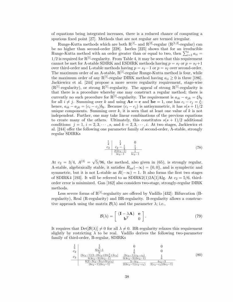
of equations being integrated increases, there is a reduced chance of computing aspurious fixed point [27]. Methods that are not regular are termed irregular.
Runge-Kutta methods which are both R[1]- and R[2]-regular (R[1,2]-regular) canbe no higher than second-order [228]. Iserles [225] shows that for an irreducibleRunge-Kutta method with an order greater than or equal to two, then
∑si=1 aii =
1/2 is required for R[1]-regularity. From Table 4, it may be seen that this requirementcannot be met for A-stable SDIRK and ESDIRK methods having p = sI or p = sI+1over third-order and L-stable methods having p = sI−1 or p = sI over second-order.The maximum order of an A-stable, R[1]-regular Runge-Kutta method is four, whilethe maximum order of any R[1]-regular DIRK method having aii ≥ 0 is three [186].Jackiewicz et al. [244] propose a more severe regularity requirement, stage-wise
(R[1]-regularity), or strong R[1]-regularity. The appeal of strong R[1]-regularity isthat there is a procedure whereby one may construct a regular method; there iscurrently no such procedure for R[1]-regularity. The requirement is aik − ajk = ξbkfor all i 6= j. Summing over k and using Ae = c and be = 1, one has ci − cj = ξ;hence, aik − ajk = (ci − cj)bk. Because (ci − cj) is antisymmetric, it has s(s+ 1)/2unique components. Summing over k, it is seen that at least one value of k is notindependent. Further, one may take linear combinations of the previous equationsto create many of the others. Ultimately, this constitutes s(s + 1)/2 additionalconditions: j = 1, i = 2, 3, · · · , s, and k = 2, 3, · · · , i. At two stages, Jackiewicz etal. [244] offer the following one parameter family of second-order, A-stable, stronglyregular SDIRKs
14
14 0
c2 c2 − 14
14
2(2c2−1)4c2−1
14c2−1
(78)
At c2 = 3/4, A(3) =√
5/96, the method, also given in (65), is strongly regular,A-stable, algebraically stable, it satisfies Rint(−∞) = {0, 0}, and is symplectic andsymmetric, but it is not L-stable as R(−∞) = 1. It also forms the first two stagesof SDIRK4 [193]. It will be referred to as SDIRK2(1)2A[1]Alg. At c2 = 5/6, third-order error is minimized. Gan [162] also considers two-stage, strongly-regular DIRKmethods.
Less severe forms of R[1]-regularity are offered by Vadillo [432]: Bifurcation (B-regularity), Real (R-regularity) and BR-regularity. B-regularity allows a construc-tive approach using the matrix B(λ) and the parameter λ; i.e.,
B(λ) =
[(I− λA) e
bT 0
]. (79)
It requires that Det[B(λ)] 6= 0 for all λ 6= 0. BR-regularity relaxes this requirementslightly by restricting λ to be real. Vadillo derives the following two-parameterfamily of third-order, B-regular, SDIRKs
16
16 0 0
c26c2−1
616 0
c3(6c3−1)(3−24c2+24c22+2c3)
6(4c2−3)(6c2−1)(6c3−1)(c2−c3)3(4c2−3)(6c2−1)
16
6(2−3c2−3c3+6c2c3)(6c2−1)(6c3−1)
3−4c32(6c2−1)(c2−c3)
4c2−32(c2−c3)(6c3−1)
(80)
38
for which Det[B(λ)] = −1. There are no values of c2 and c3 that yield an A-stablemethod. Weaker still, Xiao et al. [455] defines weak R[1]-regularity that is achievedby all consistent Runge-Kutta methods.
Xiao et al. [455] also define a weak R[2]-regularity. Runge-Kutta methods thathave M > O and b ≥ 0 are weakly R[2]-regular for positive step-sizes. In terms ofHopf bifurcations, Iserles et al. [228] state that symplectic Runge-Kutta methodswith positive weights, bi ≥ 0, are R[H]− regular. Further, a consistent Runge-Kuttamethod is R[H] − regular if and only if R(z) is symmetric [R(z)R(−z) = 1 or (64)],and the method is A-stable. Methods that are R[1,2,H]-regular are termed strictlyregular.
2.12 Boundary and Smoothness Order Reduction
A common application of DIRK-type methods is to semidiscretized PDEs. Theresulting initial boundary value problem (IBVP) solution may fail to exhibit theclassical global convergence rate that one might expect. Crouzeix [120,123] appearsto have been the first to point this out. The phenomenon is attributable to thespatial boundaries (space-time problems) due to the interaction of the boundaryconditions with the low stage-order information. It may also occur due to a lack ofspatial smoothness of the RHS for the same reason. The degree of order reductiondepends on the type of problem being integrated, the type of boundary conditionbeing applied and the spatial smoothness of the solution. A cursory summary ofboundary and smoothness order reduction results relevant to DIRK-type methodsis provided, focusing primarily on its severity under different circumstances. Globalconvergence rates generally appear as the minimum of the classical order p and thestage-order q, plus some constant, i.e., a best- and worst-case scenario.
Boundary order reduction of implicit Runge-Kutta methods in the context oflinear equations, u′(t) = A(t)u(t) + f(t) (nonautonomous) and u′(t) = Au(t) + f(t)(autonomous), is the best understood. One of the earliest efforts on this mat-ter was by Verwer [437]. He considers the implicit Euler, the one-stage, second-order Gauss method, SDIRK-NCS23 and SDIRK-NC34 methods on the nonhomo-geneous problem using either homogeneous or inhomogeneous Dirichlet boundaryconditions. Empirically derived global convergence rates were Min(p, q + 2 + 1/3)and Min(p, q + 1 + 1/4) in these two cases, respectively. If the value of A wasnonsmooth, this is further reduced to Min(p, q + 1). Ostermann and Roche [328]performed an analytical study of the autonomous nonhomogeneous problem, requir-ing A(α)-stable methods and, under certain restrictions, derived global convergencerates. For step-sizes h0 ≤ h ≤ H, homogeneous boundary conditions gave riseto global convergence rates of Min(p, q + 2 + ν), while nonhomogeneous conditionsyielded Min(p, q + 1 + ν). The reader is referred to Ostermann and Roche [328]for the definition of nu. Smaller step-sizes h ≤ h0 return the classical convergencerate p. Refining this, Lubich and Ostermann [290] solved the one-dimensional in-homogeneous heat equation and determined global order to be Min(p, q + 1 + β).Dirichlet conditions produced β = 5/4 and β = 1/4 in the homogeneous and inho-mogeneous cases, respectively. Corresponding results for Neumann conditions were
39
found to be β = 7/4 and β = 3/4. Increasing the dimensionality and consideringthe nonautonomous problem, Lubich and Ostermann [292] find that the convergencerate is unaffected by periodic boundary conditions; however, Neumann conditionshave lower convergence rates, Min(p, q+ 1 + β), in two and three dimensions whereβ = 1/4, than in one dimension where β = 5/4. Lubich and Ostermann [293]then showed that the boundary order reduction was confined to the boundary, andthat the interior manifested superconvergence to the classical order of the method.Nonsmooth data also exhibited localized order reduction. Results from each ofthese papers assumed an invertible A-matrix and strongly A(α)-stable methods.Zouraris [467] derives a global convergence rate of Min(p, q + 1 + 1/2) for SDIRK-NC34 solving the nonautonomous problem with Neumann conditions. In the caseof variable step-sizes applied to the nonautonomous problem, Gonzalez and Oster-mann [169] show that results are similar to the fixed step-size case. Using a differentanalysis tool than Ostermann and Roche [328], Alonso-Mallo and Palencia [15] con-sider A(α)-stable methods but only require that the lower left (s−1)× (s−1) blockof the A-matrix be invertible (thus allowing EDIRKs, ESDIRKs and QESDIRKs).On nonhomogeneous hyperbolic and parabolic problems, the global convergence ratewas determined to be Min(p, q + 1 + ν) for |R(−∞)| < 1 and Min(p, q + ν + ν/m)for |R(−∞)| = 0 where m is the multiplicity of the root at z = −∞ for the func-tion R(z) − 1 = 0. Test problems using SDIRK-NC34 and homogeneous Dirichletconditions on the autonomous parabolic equations showed 0 ≤ ν ≤ 5/4. Inhomoge-neous boundary conditions lowered this to 0 ≤ ν ≤ 1/4. Solving an inhomogeneoushyperbolic equation with inhomogeneous Dirichlet conditions showed 0 ≤ ν ≤ 1/2.Trompert and Verwer [429] consider order reduction on linear PDEs in the presenceof local spatial grid refinement while using a stage-order two ESDIRK.
To address the boundary order reduction associated with linear problems, cor-rective action may take place with the Runge-Kutta coefficients of the scheme or bycorrecting each of the stage and step values. To date, we are not aware of any effortsto remedy boundary order reduction by using Butcher coefficients for DIRK-typemethods. Koto [264] does this with explicit Runge-Kutta methods but the resultingmethods are relatively inefficient. Lubich and Ostermann [291] provide additionalorder conditions to deal with boundary order reduction for methods closely re-lated to DIRK-type methods, Rosenbrock methods. Recently, Alonso-Mallo [11,12],Alonso-Mallo and Cano [13], and Calvo and Palencia [86] devise alternative cor-rective procedures applied to algebraically stable SDIRKs to retrieve full temporalconvergence rates.
Fewer results exist on semilinear, quasilinear and nonlinear problems. Verwer[437] solves Burgers’ equation numerically by using SDIRK-NCS23 and SDIRK-NC34 and he empirically observes global convergence rates of Min(p, q + 2 + 2/3)and Min(p, q+ 1 + 1/4) with homogeneous and inhomogeneous Dirichlet conditions,respectively. For a nonlinear problem with nonsmooth coefficients, this convergencerate was reduced to Min(p, q + 1). Lubich and Ostermann [292] conclude that,with the possible exception of 3-D problems using Neumann boundary conditions,results for quasilinear problems u′(t) = A(u(t))u(t) + f(t) were the same as thosefor linear nonautonomous problems. For semilinear problems u′(t) = A(t)u(t) +
40
g(t, u(t)), Lubich and Ostermann [290] find that homogeneous Dirichlet conditionsyields Min(p, q + 1 + 3/4) on the semilinear problem but Min(p, q + 1 + 5/4) onthe linear problem. Nonlinear equations exhibit boundary order reduction mostseverely. Ostermann and Thalhammer [329] study strongly A(α)-stable methodsapplied to parabolic nonlinear equations and obtain convergence rates of Min(p, q+1)independent of whether the step-size was fixed or not. Calvo et al. [81] providea method for avoiding order reduction on nonlinear problems when using IMEXadditive Runge-Kutta methods. The implicit portion of these third- and fourth-order IMEX methods are SDIRKs padded with a column of zeros (ai1 = 0, i =1, 2, . . . , s).
2.13 Efficiency
Quantifying the efficiency of DIRK-type methods for purposes of comparing meth-ods is far more difficult than it is for explicit Runge-Kutta methods [256]. Becausethe methods are ideally never stability bound, one may focus on accuracy efficiencyalone, i.e., the work required per unit of physical time at fixed integration error. Todo this, however, one must quantify both accuracy and work. If there is no orderreduction, accuracy of methods may be compared by using the leading order trunca-tion error, A(p+1). In the presence of order reduction, the proper analogue of A(p+1)
is not clear. Matters are made even more difficult on stiff problems because one isconfronted with different accuracies for the differential variables and the emergingalgebraic variables. Measuring work of a method may be affected by many thingsthat are intrinsic to the overall method, including the magnitude of γ, the spacing ofthe abscissae, the quality of the stage-value prediction, the stage-order and the manystability characteristics of the method. It is also affected by issues not intrinsic tothe method, including iteration control and the implementation strategy. In certaincases, confluent methods may reduce work because the iteration on the second stage,having the repeated abscissae, begins with a high-quality starting guess. Succeedingat measuring work would also benefit a variable-order implementation. Capitulatingon a quantitative measure of relative efficiency, several qualitative guidelines seemreasonable. Small values of γ, high stage-order, L-stability, internal stability coupledwith high-quality stage-value predictors and iteration control are likely to enhanceefficiency. Some work savings are also possible when using stiffly-accurate EDIRK,ESDIRK and QESDIRK methods by stage-derivative reuse [324].
2.14 Solvability
Before proceeding to solve for the stage- and step-values, U [i] and U [n+1], it would beprudent to understand under what conditions the coupled nonlinear stage and stepequations possess a unique solution [76, 77, 80, 129, 193, 269, 470]. If the equationsdo possess a unique solution, the method is termed feasible [410]. For inner prod-uct norms and differential equations having a one-sided Lipschitz constant ν, thenonlinear stage equations of DIRK or SDIRK method, having positive aii, possess aunique solution for step-sizes given by [193, 302] ν∆t < Min
(a−1ii
), i = 1, 2, · · · , s.
For EDIRKs, ESDIRKs and QESDIRKs, where a11 = 0 and aij is not invertible,
41
the previous result is likely to still apply, but with i = 2, 3, · · · , s [193]. To make thisrelation practical, one must estimate the value of ν for their problem. We are notaware of any code that explicitly uses this criterion as part of a step-size algorithm.Calvo et al. [80] consider this same topic by using the maximum norm but offer nocomparable result for DIRK-type methods. Kraaijevanger [266] also considers themaximum norm and discusses solvability for both unconditionally and conditionallycontractive methods.
2.15 Implementation
Depending on the size of the equation system, one solves the implicit algebraicequations in different ways. For small systems of equations, one generally usesdirect solvers. In this case, using the definition Fj = F
(Uj , t
[n] + cj∆t), one must
solve
Ui = U [n] +Xi + (∆t)aiiFi, Xi = (∆t)i−1∑j=1
aijFj , 1 ≤ i ≤ s (81)
where Xi is explicitly computed from existing data. Combining (81) with an appro-priate starting guess, a modified Newton iteration [180, 210, 371, 372, 378] providesUi and Fi. This is accomplished by solving
(I − (∆t)aiiJ) (Ui,k+1 − Ui,k) = −(Ui,k − U [n]
)+ Xi + (∆t)aiiFi (82)
where the subscript k denotes the value on the kth iteration, (∂F/∂U) = J is theJacobian, I is the identity matrix, (I− (∆t)aiiJ) = N is the (Newton) iterationmatrix, and (Ui,k+1 − Ui,k) = di,k is the displacement. The RHS of (82) is calledthe residual, ri,k where
Ndi,k = ri,k. (83)
Solving for the displacement vector is generally done using Gaussian eliminationwhere the iteration matrix is factorized into a permutation matrix P, for pivotingand a lower, L, and upper, U, triangular matrix. Shampine remarks that althoughthe iteration matrix for stiff problems is often ill-conditioned, the linear systemsassociated with it are not [377]. On the kth-iteration, one has
PLUdi,k = ri,k, Ui,k+1 = Ui,k + U−1L−1P−1ri,k. (84)
Jacobians are generally not reevaluated at each stage but rather after many stepsunless the problem is extremely stiff. The iteration is terminated when either thenormalized di,k = di,k/ (|Ui,k|+ η/ε) (displacement test) or the normalized ri,k =ri,k/ (|Ui,k|+ η/ε) (residual test) are sufficiently small [210,324,413,414],
τresid = cεε ≤ ||ri,k||, or, τdispl = cεε ≤ ||di,k||, cε ≈ 0.005− 0.1, (85)
where ε is the user-specified integration relative error tolerance, η is the user-specifiedintegration absolute error tolerance, cε is the tolerance ratio, and η is an absolute
42
error tolerance that need not be equal for each equation [45, 206, 343, 378]. Nørsettand Thomsen [313] investigate the proper choice for the tolerance ratio for SDIRKs.If the selected ratio is too small, then unnecessary iterations are performed; if it is toolarge, then local and global error will suffer. They select cε = 2||(b − b)TA−1||−1
where they consider embedded methods having order p + 1. Displacements (andresiduals) may be evaluated in either an L∞ or an L2 norm,
||di,k||∞ = maxi|di,k| , ||di,k||2 =
√√√√ 1
N
N∑i=1
(di,k)2. (86)
Hindmarsh [206, 377] chooses the displacement test for LSODE [343] because theresidual magnifies the error in the stiff ODE case. Two slightly different convergencerates may be defined as
ρm = (||di,m||/||di,1||)1/m , αk = ||di,k||/||di,k−1||, α = maxk
αk (87)
In PVODE [206], the convergence test is R||di,k||2 < 0.1ε where R is a constant givenin the reference [206]. DASSL [45] requires that ρm
1−ρm ||di,m||2 < ε/3. Hairer andWanner [193] use αk
1−αk ||di,k||2 ≤ cεε. Houbak et al. [210,313] suggest a combinationof displacement and residual tests. Shampine [372] insists that accepting an iterationbased on a displacement test must be accompanied by a convergence rate α ofless than unity. Hence, at least two iterations must be computed. Shampine [372]advocates α as the most accurate indicator of convergence rate. Divergence is definedas a convergence rate of αk > 2 by Hindmarsh [206], αk > 1 by Shampine [372], andρm > 0.9 by Brenan et al. [45]. For stiffly-accurate, first-stage explicit DIRK-typemethods, Olsson and Soderlind [324] recommend stage derivative reuse; the valuesof Fs = F [n+1] at the end of one step are used immediately as F1 in the followingstep.
In mildly stiff cases where either the time step or aii are changing rapidly butthe Jacobian is still sufficiently accurate, computational savings are possible. Thescaled iteration matrix is defined
Ns =−1
aii(∆t)N =
[J− 1
aii(∆t)I
](88)
for the purposes of changing either aii or (∆t) cheaply. Equation (82) is modifiedaccordingly. Following Enright [141], decomposing Ns into a lower triangular ma-trix, its inverse and an upper Hessenberg matrix, Ns = LHL−1, one may updateNs with updated (aii)2 or (∆t)2 via
J− 1
(aii)2(∆t)2I = L
[H +
(aii)2(∆t)2 − (aii)1(∆t)1
(aii)1(aii)2(∆t)1(∆t)2
I
]L−1. (89)
An alternative procedure has been given by Krogh [206,275,462]. Instead of solvingfor the displacement as suggested above, a constant c is computed and a modifiedprocedure is solved:
d(i)k = cU−1L−1P−1r
(i)k , c =
2(aii)1(∆t)1
(aii)1(∆t)1 + (aii)2(∆t)2. (90)
43
Either of these procedures may be useful in the implementation of DIRK, EDIRK,or QESDIRK methods where nonzero diagonal elements may have different values.Al-Rabeh [16] constructs p(p+ 1) pairs with aii = γ left as a free parameter. As thestep size is changed, γ is changed, within reason, such that the product containedwithin the iteration matrix γ(∆t) remains fixed.
In the event that the system of ODEs becomes nonstiff intermittently during thecomputation, one may wish to perform stiffness switching [65,314,338]. The idea isto switch between a Newton-type iteration and a fixed-point, or Picard iteration, oreven an explicit Runge-Kutta method. To do this, one first estimates the value of theLipschitz constant for the problem at hand as ||J||2 or, less precisely but more easily,as ||J||∞. By selecting (∆t) to satisfy some error tolerance, stiffness is then defined as(∆t)||J||2 � 1 [129,286,373,376,414]. Given that fixed-point iteration converges for(∆t)aii||J||2 < 1, for values larger than unity, a Newton iteration is used; for valuesless than unity, a fixed point iteration is used. Van der Houwen and Sommeijer [214]propose an intermediate solution, called approximate factorization iteration, forcases where (∆t)||J||∞ is small. They switch between iteration procedures basedon the value of aii(∆t)||J||∞. Fixed-point iteration is used for aii(∆t)||J||∞ < a,approximate factorization is used for a ≤ aii(∆t)||J||∞ < b and Newton iterationis used for b ≤ aii(∆t)||J||∞, with a = 1/2 and b = 3. A complicating factor inthis approach is that the estimation of the stiffness may be inaccurate. Higham andTrefethen [198] contend that the true characterization of stiffness comes not fromthe spectra of the Jacobian but its pseudospectra and the two may be different.
One further issue relevant to implementation using direct methods is the com-putation of the Jacobian. One may use a numerically generated Jacobian by usingfinite-difference techniques or use an analytically derived one [378]. It is a commonlyheld belief that an analytical Jacobian should be used whenever possible. Petzoldcomments that the numerical Jacobian is the weakest part of the DASSL code [45].For certain problems, a numerical Jacobian can never be expected to work. A rela-tively recent development towards analytical Jacobians is automatic differentiationtools applied directly to the source code. These tools are available for FORTRAN77 [40], FORTRAN 90 [341], and C [41]. When an analytical Jacobian is not feasibleand a numerical one must be considered, one must compute
∂Fi∂Uj
≈ F (Ui + ∆jej)− F (Ui)
∆j, (91)
where ej = {0, 0, · · · , 1, · · · , 0, 0}T is composed of only zeros except a single 1 in thejth-position. Its is apparent from the context in which it is used. The difficultiesinvolved are choosing an appropriate ∆j and computing the Jacobian expeditiously.Most codes choose ∆j based on some variation of ∆j =
√u Max (|Uj |, η), where u
is related to machine precision. It is the smallest number such that 1 +u > 1 on thecomputer of interest. To avoid division by zero, η is some absolute error tolerance.LSODE [343] and DASSL [45] offer slight variations on this idea.
Salane [349] offers a more sophisticated approach to compute a good ∆j . First, hedefines U(ref) as a U-vector constructed using representative values of the elements.
44
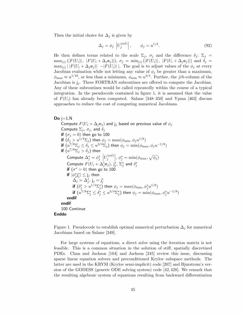
Then the initial choice for ∆j is given by
∆j = φj
∣∣∣U (ref)j
∣∣∣ , φj = u1/2. (92)
He then defines terms related to the scale Σj , σj and the difference δj ; Σj =max(i) (|F (Ui)| , |F (Ui + ∆jej)|), σj = min(i) (|F (Ui)| , |F (Ui + ∆jej)|) and δj =max(i) | |F (Ui + ∆jej)| −|F (Ui)| |. The goal is to adjust values of the φj at everyJacobian evaluation while not letting any value of φj be greater than a maximum,φmax ≈ u1/10, or less than a minimum, φmin ≈ u3/4. Further, the jth-column of theJacobian is jj . Three FORTRAN subroutines are offered to compute the Jacobian.Any of these subroutines would be called repeatedly within the course of a typicalintegration. In the pseudocode contained in figure 1, it is assumed that the valueof F (Ui) has already been computed. Salane [348–350] and Ypma [463] discussapproaches to reduce the cost of computing numerical Jacobians.
Do j=1,NCompute F (Ui + ∆jej) and jj based on previous value of φjCompute Σj , σj , and δjif (σj = 0) then go to 100if (δj > u1/4Σj) then φj = max(φmin, φju
1/8)if (u7/8Σj ≤ δj ≤ u3/4Σj) then φj = min(φmax, φju
−1/8)if (u7/8Σj > δj) then
Compute ∆∗j = φ∗j
∣∣∣U (ref)j
∣∣∣, φ∗j = min(φmax,√φj)
Compute F (Ui + ∆∗jej), j∗j , Σ∗j and δ∗j
if (σ∗ = 0) then go to 100if |φ∗j j∗j | ≤ jj then
∆j = ∆∗j , jj = j∗jif (δ∗j > u1/4Σ∗j ) then φj = max(φmin, φ
∗ju
1/8)
if (u7/8Σ∗j ≤ δ∗j ≤ u3/4Σ∗j ) then φj = min(φmax, φ∗ju−1/8)
endifendif100 Continue
Enddo
Figure 1. Pseudocode to establish optimal numerical perturbation ∆j for numericalJacobians based on Salane [349].
For large systems of equations, a direct solve using the iteration matrix is notfeasible. This is a common situation in the solution of stiff, spatially discretizedPDEs. Chan and Jackson [104] and Jackson [245] review this issue, discussingsparse linear equation solvers and preconditioned Krylov subspace methods. Thelatter are used in the KRYSI (Krylov semi-implicit) code [207] and Bjurstrøm’s ver-sion of the GODESS (generic ODE solving system) code [42, 428]. We remark thatthe resulting algebraic system of equations resulting from backward differentiation
45
formulae (BDF) methods is essentially identical to those resulting from DIRK-typemethods. Rather than the modified Newton method that is used for small sys-tems of equations, one usually considers inexact Newton methods for larger systemsof coupled equations [207, 254, 344]. The implementation of this inexact Newtonmethod in PVODEs is described by Hindmarsh [206]. Jothiprasad et al. [248] com-pare nonlinear multigrid with two variants of an inexact Newton scheme while usingan ESDIRK method to solve the compressible Navier-Stokes equations. Isono andZingg [240] contrast an approximate factorization algorithm with a Newton-Krylovalgorithm in the study of unsteady, compressible flows using the same ESDIRK.In a further study with the ESDIRK from ARK4(3)6L[2]SA [255], Bijl and Car-penter [37, 95] combine a multigrid solution strategy followed by a Newton-Krylovmethod to achieve a 30 percent speed-up.
Variable-order implicit Runge-Kutta implementations are possible but are farless common than similar multistep implementations. Cash and Liem [102] andCameron [92] do this with SDIRKs, Burrage et al. [54] use SIRKs, Butcher et al. [71]consider DESI methods, and Hairer and Wanner [194] use the Radau IIA family ofmethods. Hairer and Wanner state that the objective of such implementations is tominimize the local error per unit step. The required step-size is estimated for eachcandidate method and then the cost of this step-size is estimated. One then selectsthe method with the lowest cost to step-size ratio. As the optimal γ changes forSDIRKs and ESDIRKs as order and the number of stages changes, an embeddedapproach like the ones Cash and Liem and Burrage et al. use seems less thanideal. With increased efficiency as the goal, a variable-order strategy would bestbe incorporated into the iteration control strategy. Possibly the reason why so fewvariable-order implicit Runge-Kutta codes exist is the difficulty in executing thiswell. Butcher [63] describes an order selection strategy for variable-order methods.
In certain contexts, implicit methods may be implemented to mimic IMEX meth-ods. Brown and Hindmarsh [46] effectively consider solving (82) by treating the RHSas if all terms were to be integrated implicitly but constructing the Jacobian by usingonly the stiff part of the RHS.
2.16 Step-Size Control
Local integration error for Runge-Kutta methods is usually controlled by first cre-ating a local error estimate via an embedded method. This error estimate is thenfed to an error controller, that adjusts the time step in order to maintain some user-specified relative error tolerance ε. Ideally, this step-size estimate is used as partof an iteration control strategy. Although this review focuses on largely cost-freeembedded methods where p = p+ 1, some papers use p = p− 1 [7,16,17,209]. Oth-ers [17, 382] include the possibility of using extra function evaluations to increasethe order of their embedded method. The reliability of this error estimate may befacilitated by using L-stable main and embedded methods [179] as well as higherstage-order methods. Given noisy data, Krogh [274] describes a step-size selectionstrategy that uses a least-squares fit of past data. Ilie et al. [223] approach opti-mal time step locations during the integration of both initial and boundary value
46
problems by considering a grid deformation map, t = Θ(τ). In this formulation,each time step location in the deformed space is equispaced relative to adjacent steplocations but variable in the undeformed space. The goal is to determine an optimalgrid deformation map, through a variational approach, which either 1) minimizesthe work required to maintain a specified local error tolerance or 2) minimizes thelocal error given a fixed amount of work (steps).
Following Soderlind [402–405], we consider several error-control strategies of theform
(∆t)[n+1] = κ(∆t)[n]
{ε
||δ[n+1]||
}α{ ||δ[n]||ε
}β {ε
||δ[n−1]||
}γ×
×
{(∆t)[n]
(∆t)[n−1]
}a{(∆t)[n−1]
(∆t)[n−2]
}b
(93)
for p(p)-pairs (p = p− 1). In (93), κ ≈ 0.95 is the safety factor, (∆t)[n−i] = t[n−i] −t[n−i−1] is the step size, and δ[n+1] is the vector of most recent local error estimatesof the integration from t[n−1] to t[n] associated with the computation of U [n+1]. Toanalyse this controller, Soderlind defines two polynomials P (q) = αq2 − βq + γ andQ(q) = q2 − aq − b where it is required that deg P (q) ≤ deg Q(q). If commonfactors are contained in both P (q) and Q(q) then they are removed. ¿From this,the characteristic polynomial or characteristic equation of the controller, having nocommon factors between P (q) and Q(q), is
Φ(q) = (q − 1)Q(q) + pP (q) = q3 + (pα− a− 1) q2
+ (−pβ + a− b) q + (pγ + b) . (94)
For stability, all roots of Φ must have a magnitude of less than or equal to one.Controllers based on this structure possess three distinct orders: the order of thedynamics, pD; the order of adaptivity, pA; and the order of the step-size filter, pF .Soderlind names particular controllers as HpDpApF . The degree of the polynomialΦ is the order of the dynamics, while the order of adaptivity determines the rateat which the local error is adapted to the error tolerance. The filter order is re-lated to averaging of the potentially noisy data and, when greater than zero, thecontroller acts as a low-pass step-size filter by removing high frequency data. Assmall roots to the characteristic equation are sometimes desirable, one may enforce(pα− a− 1) = 0, (−pβ + a− b) = 0 and (pγ + b) = 0 to obtain Φ = (q − 0)3. Thisimplies α = (a + 1)/p, β = (a − b)/p and γ = −b/p and that all roots vanish.Controllers satisfying these equations are denoted H0pDpApF . Methods posessingthird-order dynamics are of particular interest. Within this class, one may designH312 [β = −2α, γ = α], H321 [b = (1− a), γ = −(α+ β)] and H330 [a = 2, b = −1]controllers, but HpDpApF controllers having pD < pA + pF do not appear to exist.Table 8 lists coefficients for various controllers. A more exhaustive list is given bySoderlind [404] as well as further design details. As the characteristic polynomialroot positions play an important role in controller behavior, we note the pD-rootsof several controllers: H211 {1/2 ± I/2}, PPID {0.4838 ± 0.3275I, 0.7325}, H321
47
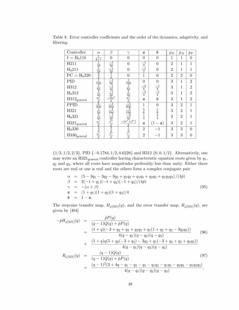
Table 8. Error controller coefficients and the order of the dynamics, adaptivity, andfiltering.
Controller α β γ a b pD pA pFI = H0110 1
p+1 0 0 0 0 1 1 0
H211 14p
−14p 0 −1
4 0 2 1 1
H0211 12p
−12p 0 −1
2 0 2 1 1
PC = H0220 2p
1p 0 1 0 2 2 0
PID 118p
−19p
118p 0 0 3 1 2
H312 18p
−14p
18p
−38
−18 3 1 2
H0312 14p
−12p
14p
−34
−14 3 1 2
H312generalα∗
p−2α∗
pα∗
p a b 3 1 2
PPID 620p
−120p
−520p 1 0 3 2 1
H321 13p
−118p
−518p
56
16 3 2 1
H0321 54p
−12p
−34p
14
34 3 2 1
H321generalα∗
pβ∗
p−(α∗+β∗)
p a (1− a) 3 2 1
H0330 3p
3p
1p 2 −1 3 3 0
H330generalα∗
pβ∗
pγ∗
p 2 −1 3 3 0
{1/3, 1/2, 2/3}, PID {−0.1784, 1/2, 0.6228} and H312 {0, 0, 1/2}. Alternatively, onemay write an H321general controller having characteristic equation roots given by q1,q2 and q3, where all roots have magnitudes preferably less than unity. Either threeroots are real or one is real and the others form a complex conjugate pair
α = (5− 3q1 − 3q2 − 3q3 + q1q2 + q1q3 + q2q3 + q1q2q3) /(4p)β = 2(−1 + q1)(−1 + q2)(−1 + q3)/(4p)γ = −(α+ β)a = (1 + q1)(1 + q2)(1 + q3)/4b = 1− a.
(95)
The step-size transfer map, Hϕ[321](q), and the error transfer map, Rϕ[321](q), aregiven by [404]
−pHϕ[321](q) =pP (q)
(q − 1)Q(q) + pP (q)
=(1 + q)(−3 + q2 + q3 + q2q3 + q1(1 + q2 + q3 − 3q2q3))
4(q − q1)(q − q2)(q − q3)(96)
+(1 + q)q(5 + q2(−3 + q3)− 3q3 + q1(−3 + q2 + q3 + q2q3))
4(q − q1)(q − q2)(q − q3)
Rϕ[321](q) =(q − 1)Q(q)
(q − 1)Q(q) + pP (q)(97)
=(q − 1)2(3 + 4q − q1 − q2 − q3 − q1q2 − q1q3 − q2q3 − q1q2q3)
4(q − q1)(q − q2)(q − q3).
48
One may also consider the control map of the controller [404]
C(q) =P (q)
(q − 1)Q(q). (98)
As with the H321general controller, one may also write an H312general as
α = −(q1 − 1)(q2 − 1)(q3 − 1)/(4p)β = −2αγ = αa = (3(−1 + q3) + q2(3 + q3) + q1(3 + q2 + q3 − q2q3)) /4b = (−1 + q2 + q3 − q2q3 − q1(−1 + q2 + q3 + 3q2q3)) /4
(99)
and
−pHϕ[312](q) =−(1 + q)2(q1 − 1)(q2 − 1)(q3 − 1)
4(q − q1)(q − q2)(q − q3),(100)
Rϕ[312](q) =(q − 1)(4q + (−1 + q2)(−1 + q3) + q1(−1 + q2 + q3 + 3q2q3)
4(q − q1)(q − q2)(q − q3)
+q(q − 1)(3 + q1(−3 + q2(−1 + q3)− q3)− 3q3 − q2(3 + q3))
4(q − q1)(q − q2)(q − q3).
(101)
In the event that one needs higher-order adaptivity or filtering, one may consider amore general controller than (93) by multiplying the RHS by{
||δ(n−2)||ε
}δ {ε
||δ(n−3)||
}ε{(∆t)(n−2)
(∆t)(n−3)
}c{(∆t)(n−3)
(∆t)(n−4)
}d
. (102)
If this is done, one might best include the step-size ratio dependence of α, β, γ, δ andε that occurs with controllers using γ, δ, ε, · · · otherwise the delivered controllerbehavior in cases where the step-size ratio deviates significantly from unity maybe different from the design intent. In the event of order reduction, p no longerreflects the actual order of the embedded method. Controller coefficients might bestbe considered so that the controller functions well when given either the formal oractual value of p. Order conditions for the adaptivity and filter are
pA = 2 a = 1− b− c− dpA = 3 b = −1− 2c− 3d,pA = 4 c = 1− 3dpA = 5 d = −1
pF = 1 α = −β − γ − δ − εpF = 2 β = −2γ − 3δ − 4εpF = 3 γ = −3δ − 6εpF = 4 δ = −4ε.
(103)
49
Using these along with P (q) = αq4−βq3+γq2−γq+ε andQ(q) = q4−aq3−bq2−cq−d(with common factors between P (q) and Q(q) removed), one may construct thecharacteristic polynomial of the controller and generate a controller having desirableroots.
In the simplest case, the local error estimate is given by δ[n+1] = U [n+1]− U [n+1].There are two ways in which this might be improved. Normalization of the errorsfrom each equation makes particular sense when elements of the integration vectorhave different orders of magnitude. To avoid division by zero, one adds a smallpositive absolute error tolerance, η, to the denominator [45, 206, 343, 378]. Hence,the two equivalent expressions
δ[n+1] =U [n+1] − U [n+1]
|U [n+1]|+ ηε
,δ[n+1]
ε=U [n+1] − U [n+1]
ε|U [n+1]|+ η. (104)
A scalar measure of δ[n+1] is often obtained by using either an L∞ or an L2 norm,
||δ[n+1]||∞ = maxi
∣∣∣δ[n+1]i
∣∣∣ , ||δ[n+1]||2 =
√√√√ 1
N
N∑i=1
(δ
[n+1]i
)2, (105)
where N is the number of equations being integrated. When stiff equations are beingintegrated, some error estimators are prone to gross overestimation of the local error.This overestimation is related to the stability function of the embedded method asz → −∞. When R(−∞) is nonzero for stiff scaled eigenvalues, Shampine andBaca [209, 379] recommend multiplying the traditional estimate by inverse powersof the (Newton) iteration matrix. Defining m by(
R(z)− R(z)
exp(z)−R(z)
)= O(zm), <(z) < 0, z → −∞ (106)
one computes the error estimate by
δ[n+1] = N−m
(U [n+1] − U [n+1]
|U [n+1]|+ ηε
), (107)
where N−1 = U−1L−1P−1 from (84). If multiple equations are being solved, anerror controller for each equation may be required, including a tailored value of η.The motivation for doing this is that each value of δ[n+1], δ[n] and δ[n−1] in (93)might otherwise be a value from a different equation, resulting in an erratic errorhistory. Generally, one also places limits on how quickly the step-size is allowedto vary. Increases or decreases of a factor of less than five in any given step areprudent [378]. Increases greater than a factor of two may be at odds with robuststage-value predictors, error control and iteration control. Hindmarsh [206] allowsLSODE to increase the step-size up to a factor of 10 000 on the first step but limitsthis increase to 10 afterwards. VODE limits reductions in step-size to 1/10. Insituations where the future step-size selected by the controller is nearly equal to the
50
current step-size, some codes make no change to the step-size until some thresholdof, often, +20 percent is exceeded. Soderlind [403] strongly discourages introducingsuch a dead-zone because, when the controller is eventually invoked, the strongactions may cause error overshoots and step rejections.
Although never applied to implicit Runge-Kutta methods, the p(p− 2)-pair ap-proach of Tsitouras and Papakostas [431] is appealing. They consider a modifiedI-controller,
(∆t)[n+1]I = κ(∆t)[n]
{ε
f2(∆t)||δ[n+1]||
} 1p+1
, (108)
where f2 ≈ 10 is experimentally optimized. More sophisticated incarnations of thisstrategy are certainly possible and would allow one to design main scheme methodsthat were less compromised by demands of the embedded method. An alternativeapproach is to use two-step embedded methods [176] to enable higher order andbetter stability. Beyond control of local error, one might wish to control globalerror. The literature contains limited guidance on global error estimation of implicitRunge-Kutta methods applied to stiff problems [124,144,307,361,363,375,417].
Because machine precision is finite, the preceding approaches must be appliedrespecting this limit. If |U [n+1]| becomes very small, then an absolute error toleranceis added to the error estimate. Further, there are limits on how strict an errortolerance [343] or how small of a step-size may be rationally set [370]. Related tothis limit is the selection of an initial step size [45, 165, 167, 193, 206, 313, 343, 445].If the chosen step-size is too large, then the error will be excessive or the iterationmay not converge. If the chosen step-size is too small, then an inefficiency is addedor the result is swamped by rounding error. Rounding error may be minimized byusing compensated summations [69,189,199,346].
Traditionally, the embedded method is distinct from the main method becausethere are two sets of scheme weights, bi and bi. A disadvantage to this approachwhile solving stiff ODEs is that the error estimate has the stability function of anexplicit method. One could follow the strategy of Shampine and Baca, (107), andmultiply the resulting error estimate times the appropriate inverse power of theiteration matrix. However, to improve on this process, Al-Rabeh [17] and others[8, 89, 281, 450, 451] consider what one may call internal error-control as opposedto the traditional external error-control. Internal error control is often performedwithin the context of DAEs and is accomplished by imposing all embedded methodconstraints on one of the stages, often the penultimate stage, to avoid fixing γ and topermit higher order methods. The resulting error estimate is likely relatively reliableif the internal stability of the penultimate stage is controlled. When combined withthe stiffly-accurate assumption, unfortunately, the method becomes confluent. Apotential drawback of this approach is when significant order reduction occurs, eachmethod reduces to the same order because they share the same stage order. Asthe stiffness primarily affects the order of the stiff modes [157], the two solutionswill probably not collide. It is an interesting question whether there is any benefitto generating both an internal and an external error estimate. Several proposed
51
methods in this paper offer both in the event the construct is helpful, possibly usingthe difference as a measure of stiffness or order reduction.
2.17 Iteration Control
Traditionally for DIRK-type methods, the step-size is selected by using an errorestimate in collaboration with an error controller such as a P(redictive)C(ontrol)-controller. However, one must also consider how the step-size selection affects theconvergence rate of the iterative solver. Iteration control attempts to coordinate thetwo requirements of integration accuracy and iteration efficiency to yield an opti-mal time step choice throughout the computation. Gustafsson and Soderlind [180]propose a comprehensive approach to iteration control when using direct solvers.Salane [350] addresses some of these issues, but less comprehensively. Iteration con-trol strategies used in the LSODE [343], PVODE [206], and DASSL [45] softwarepackages may also be consulted. Unfortunately, little guidance exists in the litera-ture on iteration control associated with indirect solvers [206] where, arguably, mostreal-world CPU-hours are consumed.
In the case of a modified Newton iteration, Gustafsson and Soderlind contrastthe value of the iteration matrix being used to that which would exist when using acurrent step-size and fresh Jacobian. As the iteration matrix becomes more dated,they decompose the expected convergence rate of the iteration into that causedby changes in step-size from the value used to construct the iteration matrix andthat due to an increasingly inaccurate Jacobian. As one may observe the actualconvergence rate, α, and readily compute the convergence rate component due tostep-size changes, αlu
αk = ||d(i)k ||/||d
(i)k−1||, α = max
kαk, αlu =
∣∣∣∣(∆t)− (∆t)lu
(∆t)lu
∣∣∣∣ (109)
via a linearization, then αjac = α− αlu. The subscript lu denotes the value used toconstruct the most recent iteration matrix. For quantites related to the Jacobian,the subscript jac is used. Obviously, reliable estimates for the scaled displacementare essential to proper functioning of the iteration control. One then contrasts theseestimates to target values for these quantities, αref , αLU and αJAC. The goal now isto keep α ≈ αref , αlu ≈ αLU and αjac ≈ αJAC. If αjac > αJAC, then the convergenceis likely to either fail or be inefficient due to an old Jacobian. Note that with thisprocedure, one need not place a priori fixed age limits on the Jacobian or iterationmatrices as is commonly done. Gustafsson and Soderlind recommend starting withthe values αref = 0.2, αLU = 0.2 and αJAC = 0.2. Soderlind [403] recommendsαref ≤ 0.37 on lower precision calculations and reduced values as the precisionrequirement becomes more strict. With these values, they provide pseudocode forselecting the time step in conjunction with the error controller, criteria for updatingthe Jacobian, and when to update the iteration matrix, for both converging anddiverging iterations. Several improvements to this procedure have been devised byOlsson and Soderlind [323] and de Swart [423]. An abbreviated version of the latterappears in figure 2. It is invoked once the step has either been successfully completed
52
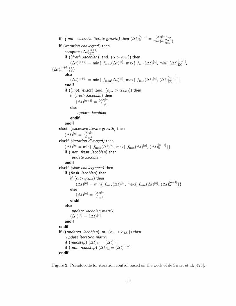
if (.not. excessive iterate growth) then (∆t)[n+1]α = (∆t)[n]αref
max{α, αreffmax
}if (iteration converged) then
compute (∆t)[n+1]EC
if ((fresh Jacobian) .and. (α > αref)) then
(∆t)[n+1] = min{ fmax(∆t)[n], max{ fmin(∆t)[n], min{ (∆t)[n+1]EC ,
(∆t)[n+1]α }}}
else(∆t)[n+1] = min{ fmax(∆t)[n], max{ fmin(∆t)[n], (∆t)
[n+1]EC }}
endifif ((.not. exact) .and. (αjac > αJAC)) then
if (fresh Jacobian) then
(∆t)[n+1] = (∆t)[n]
frigidelse
update Jacobianendif
endifelseif (excessive iterate growth) then
(∆t)[n] = (∆t)[n]
frigid
elseif (iteration diverged) then
(∆t)[n] = min{ fmax(∆t)[n], max{ fmin(∆t)[n], (∆t)[n+1]α }}
if (.not. fresh Jacobian) thenupdate Jacobian
endifelseif (slow convergence) then
if (fresh Jacobian) thenif (α > ξαref) then
(∆t)[n] = min{ fmax(∆t)[n], max{ fmin(∆t)[n], (∆t)[n+1]α }}
else(∆t)[n] = (∆t)[n]
frigidendif
elseupdate Jacobian matrix
(∆t)[n] = (∆t)[n]
endifendifif ((updated Jacobian) .or. (αlu > αLU)) then
update iteration matrixif (redostep) (∆t)lu = (∆t)[n]
if (.not. redostep) (∆t)lu = (∆t)[n+1]
endif
Figure 2. Pseudocode for iteration control based on the work of de Swart et al. [423].
53
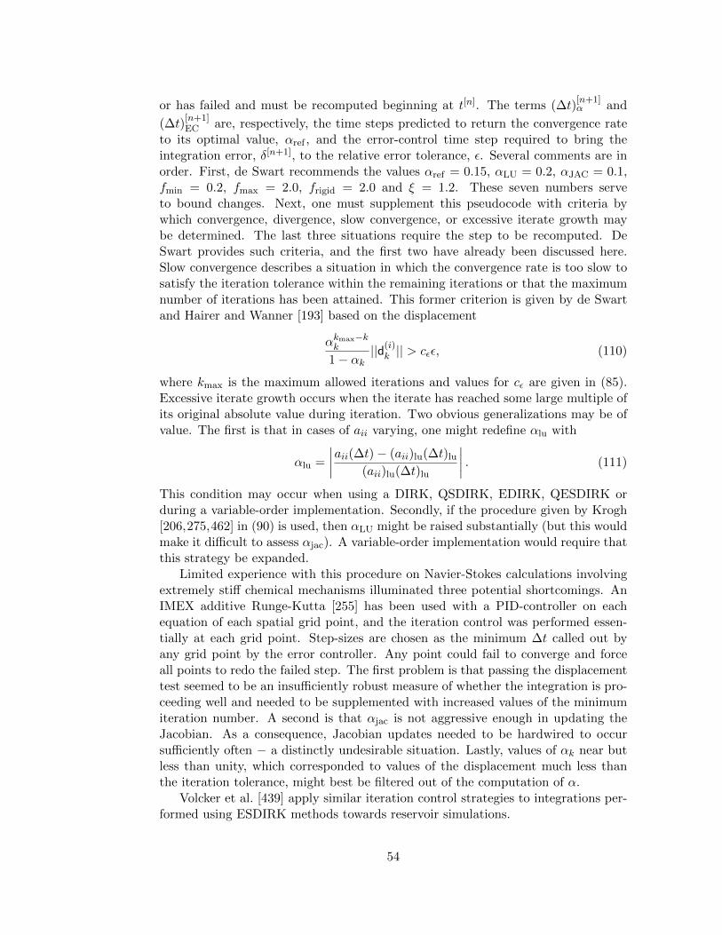
or has failed and must be recomputed beginning at t[n]. The terms (∆t)[n+1]α and
(∆t)[n+1]EC are, respectively, the time steps predicted to return the convergence rate
to its optimal value, αref , and the error-control time step required to bring theintegration error, δ[n+1], to the relative error tolerance, ε. Several comments are inorder. First, de Swart recommends the values αref = 0.15, αLU = 0.2, αJAC = 0.1,fmin = 0.2, fmax = 2.0, frigid = 2.0 and ξ = 1.2. These seven numbers serveto bound changes. Next, one must supplement this pseudocode with criteria bywhich convergence, divergence, slow convergence, or excessive iterate growth maybe determined. The last three situations require the step to be recomputed. DeSwart provides such criteria, and the first two have already been discussed here.Slow convergence describes a situation in which the convergence rate is too slow tosatisfy the iteration tolerance within the remaining iterations or that the maximumnumber of iterations has been attained. This former criterion is given by de Swartand Hairer and Wanner [193] based on the displacement
αkmax−kk
1− αk||d(i)
k || > cεε, (110)
where kmax is the maximum allowed iterations and values for cε are given in (85).Excessive iterate growth occurs when the iterate has reached some large multiple ofits original absolute value during iteration. Two obvious generalizations may be ofvalue. The first is that in cases of aii varying, one might redefine αlu with
αlu =
∣∣∣∣aii(∆t)− (aii)lu(∆t)lu
(aii)lu(∆t)lu
∣∣∣∣ . (111)
This condition may occur when using a DIRK, QSDIRK, EDIRK, QESDIRK orduring a variable-order implementation. Secondly, if the procedure given by Krogh[206,275,462] in (90) is used, then αLU might be raised substantially (but this wouldmake it difficult to assess αjac). A variable-order implementation would require thatthis strategy be expanded.
Limited experience with this procedure on Navier-Stokes calculations involvingextremely stiff chemical mechanisms illuminated three potential shortcomings. AnIMEX additive Runge-Kutta [255] has been used with a PID-controller on eachequation of each spatial grid point, and the iteration control was performed essen-tially at each grid point. Step-sizes are chosen as the minimum ∆t called out byany grid point by the error controller. Any point could fail to converge and forceall points to redo the failed step. The first problem is that passing the displacementtest seemed to be an insufficiently robust measure of whether the integration is pro-ceeding well and needed to be supplemented with increased values of the minimumiteration number. A second is that αjac is not aggressive enough in updating theJacobian. As a consequence, Jacobian updates needed to be hardwired to occursufficiently often − a distinctly undesirable situation. Lastly, values of αk near butless than unity, which corresponded to values of the displacement much less thanthe iteration tolerance, might best be filtered out of the computation of α.
Volcker et al. [439] apply similar iteration control strategies to integrations per-formed using ESDIRK methods towards reservoir simulations.
54
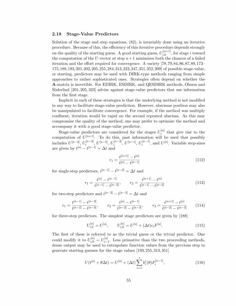
2.18 Stage-Value Predictors
Solution of the stage and step equations, (82), is invariably done using an iterativeprocedure. Because of this, the efficiency of this iterative procedure depends strongly
on the quality of the starting guess. A good starting guess, U[n+1]i,0 , for stage i toward
the computation of the U -vector at step n+1 minimizes both the chances of a failediteration and the effort required for convergence. A variety [78,79,84,86,87,89,173–175,188,193,201,202,205,255,284,313,323,347,351,352,399] of possible stage-value,or starting, predictors may be used with DIRK-type methods ranging from simpleapproaches to rather sophisticated ones. Strategies often depend on whether theA-matrix is invertible. For EDIRK, ESDIRK, and QESDIRK methods, Olsson andSoderlind [201, 205, 323] advise against stage-value predictors that use informationfrom the first stage.
Implicit in each of these strategies is that the underlying method is not modifiedin any way to facilitate stage-value prediction. However, abscissae position may alsobe manipulated to facilitate convergence. For example, if the method was multiplyconfluent, iteration would be rapid on the second repeated abscissa. As this maycompromise the quality of the method, one may prefer to optimize the method andaccompany it with a good stage-value predictor.
Stage-value predictors are considered for the stages U[n]i that give rise to the
computation of U [n+1]. To do this, past information will be used that possibly
includes U [n−3], U[n−3]i , U [n−2], U
[n−2]i , U [n−1], U
[n−1]i , and U [n]. Variable step-sizes
are given by t[n] − t[n−1] = ∆t and
r1 =t[n+1] − t[n]
t[n] − t[n−1](112)
for single-step predictors, t[n−1] − t[n−2] = ∆t and
r1 =t[n] − t[n−1]
t[n−1] − t[n−2], r2 =
t[n+1] − t[n]
t[n−1] − t[n−2](113)
for two-step predictors and t[n−2] − t[n−3] = ∆t and
r1 =t[n−1] − t[n−2]
t[n−2] − t[n−3], r2 =
t[n] − t[n−1]
t[n−2] − t[n−3], r3 =
t[n+1] − t[n]
t[n−2] − t[n−3](114)
for three-step predictors. The simplest stage predictors are given by [188]
U[n]i,0 = U [n], U
[n]i,0 = U [n] + (∆t)ciF
[n]. (115)
The first of these is referred to as the trivial guess or the trivial predictor. One
could modify it to U[n]i,0 = U
[n]i−1. Less primative than the two proceeding methods,
dense output may be used to extrapolate function values from the previous step togenerate starting guesses for the stage values [193,255,313,351]
U(t[n] + θ∆t) = U [n] + (∆t)s∑i=1
b∗i (θ)F[n−1]i , (116)
55
where θ is selected to be one of the scheme abscissae, ci. Both stability and accuracydegrade quickly as θ is increased; consequently, a limit of θ ≤ 3 is often imposed[173,175,352]. This step change restriction is not inconsistent with prudent error anditeration control strategies [423]. These methods, like those that follow, cannot beused on the first step where the trivial guess must be used. Some authors advocatehermite interpolation for stage-value predictors [7, 281].
More sophisticated approaches to stage-value prediction are now considered.Laburta [284] considers stage-value predictors that require as many as two effectiveadditional function evaluations and are of the form
U[n]i,0 = U [n−1] + (∆t)
s∑j=1
βijF[n−1]j
+ (∆t)(βi,0F
[n−1] + βi,s+1F[n] + βi,s+2F
[n−1]s+2
)(117)
U[n−1]s+2 = U [n−1] + (∆t)
s∑j=1
µjF[n−1]j
+ (∆t)(µ0F
[n−1] + µs+1F[n]), (118)
where extra function evaluations (F [n−1], F [n] and F[n−1]s+2 ) may be used to increase
the order of the predictor. Hairer et al. [188] generalize this procedure to appear as
U[n]i,0 = U [n−1] + (∆t)
s∑j=1
βijF[n−1]j + (∆t)
m∑j=1
νijF[n−1]s+j (119)
U[n−1]s+j = U [n−1] + (∆t)
s∑k=1
µAjkF[n−1]k + (∆t)
j−1∑k=1
µBjkF[n−1]k , (120)
where µij = (µAij , µBij) and ςi =
∑sj=1 µ
Aij+∑i−1
j=1 µBij . It is useful to define c = (e+rc)
and B = e ⊗ bT . Matrices βij and µAij are of dimension s × s, νij is of dimension
s ×m and µBij is of dimension s × (m − 1). It may be seen that Laburta’s methodincludes up to three additional function evaluations (m ≤ 3). Effectively, however,it has two additional function evaluations as F [n] from the previous step may be
used for F [n−1] in the current step. Order conditions for these methods, t(p)j , up to
order p = 4, may be constructed with six of the eight order conditions already given
by Hairer et al. [188] for step-size ratios of unity. For bushy trees, t(κ)1 , κ = 1, 2, 3, 4,
s∑j=1
βijcκ−1j +
m∑j=1
νijςκ−1j =
s∑j=1
Bijcκ−1j + r
s∑j=1
aijcκ−1j (121)
56
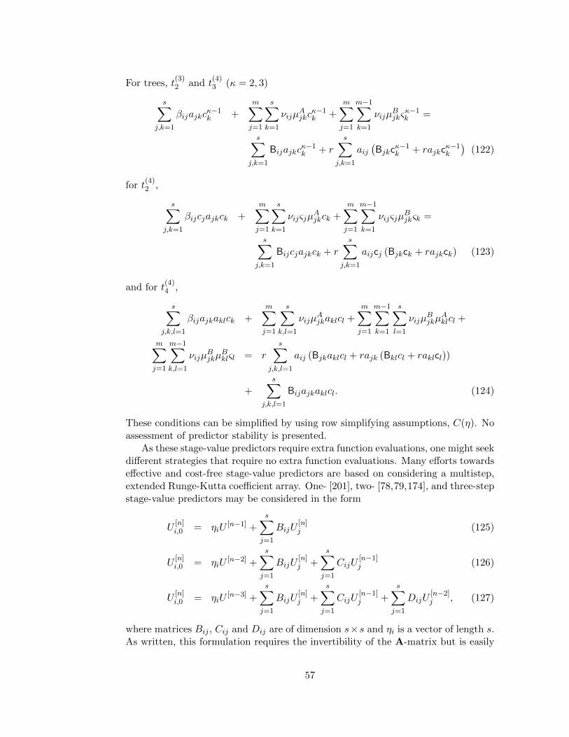
For trees, t(3)2 and t
(4)3 (κ = 2, 3)
s∑j,k=1
βijajkcκ−1k +
m∑j=1
s∑k=1
νijµAjkc
κ−1k +
m∑j=1
m−1∑k=1
νijµBjkς
κ−1k =
s∑j,k=1
Bijajkcκ−1k + r
s∑j,k=1
aij(Bjkc
κ−1k + rajkc
κ−1k
)(122)
for t(4)2 ,
s∑j,k=1
βijcjajkck +m∑j=1
s∑k=1
νijςjµAjkck +
m∑j=1
m−1∑k=1
νijςjµBjkςk =
s∑j,k=1
Bijcjajkck + r
s∑j,k=1
aijcj (Bjkck + rajkck) (123)
and for t(4)4 ,
s∑j,k,l=1
βijajkaklck +
m∑j=1
s∑k,l=1
νijµAjkaklcl +
m∑j=1
m−1∑k=1
s∑l=1
νijµBjkµ
Aklcl +
m∑j=1
m−1∑k,l=1
νijµBjkµ
Bklςl = r
s∑j,k,l=1
aij (Bjkaklcl + rajk (Bklcl + raklcl))
+
s∑j,k,l=1
Bijajkaklcl. (124)
These conditions can be simplified by using row simplifying assumptions, C(η). Noassessment of predictor stability is presented.
As these stage-value predictors require extra function evaluations, one might seekdifferent strategies that require no extra function evaluations. Many efforts towardseffective and cost-free stage-value predictors are based on considering a multistep,extended Runge-Kutta coefficient array. One- [201], two- [78,79,174], and three-stepstage-value predictors may be considered in the form
U[n]i,0 = ηiU
[n−1] +s∑j=1
BijU[n]j (125)
U[n]i,0 = ηiU
[n−2] +s∑j=1
BijU[n]j +
s∑j=1
CijU[n−1]j (126)
U[n]i,0 = ηiU
[n−3] +s∑j=1
BijU[n]j +
s∑j=1
CijU[n−1]j +
s∑j=1
DijU[n−2]j , (127)
where matrices Bij , Cij and Dij are of dimension s×s and ηi is a vector of length s.As written, this formulation requires the invertibility of the A-matrix but is easily
57

generalized to a k-step predictor. Calvo designs constant [82] and variable [87] step-size k-step predictors, requiring the invertibility of A, based on previous values ofonly one particular stage.
Single-step predictors like (125) appear first to have been considered by Sand[352] and later by many others [173,175,201,205,323,347]. Sand [352] derives orderand inverse-order conditions for a class of predictors and distinguishes between caseswhere the step-size ratio, r = (∆t)[n+1]/(∆t)[n], is either r < 0.1, 0.1 ≤ r ≤ 2.0, or2.0 ≤ r. As r increases, order is reduced and inverse order is increased. Gonzalez-Pinto et al. [174,175] conclude that at stringent tolerances, predictor order mattersbut at more lax tolerances, stability properties matter more. Both Gonzalez-Pintoet al. [174] and Calvo and Portillo [87] find that higher order starters do not alwaysoutperform lower order ones.
General one-, two- and three-step predictors are represented by using extendedButcher arrays characterized by A, b and c as
c A Oc B r1A
bT r1bT
c A O Oc B r1A Oc B r1B r2A
bT r1bT r2b
T
c A O O Oc B r1A O Oc B r1B r2A Oc B r1B r2B r3A
bT r1bT r2b
T r3bT
(128)
associated with (125), (126) and (127), where B = e ⊗ bT , eT = {e, e, · · · , e},Ae = c, O is a square matrix of zeros, and Be = e for methods that are at leastfirst-order accurate. Note that the components of c are given by c, c = e + r1c,c = e(1 + r1) + r2c and c = e(1 + r1 + r2) + r3c
c = {c, c}T , c = {c, c, c}T , c = {c, c, c, c}T . (129)
Directly related to these, diag(c) = C, diag(c) = C and diag(c) = C. We also defineβ, the last row of A, for one-, two- and three-step predictors as
β = {B, r1A}T , β = {B, r1B, r2A}T , β = {B, r1B, r2B, r3A}T . (130)
The order of accuracy of the stage-value predictor is given by
||U [n]i − U
[n]i,0 || = O
((∆t)p
), (131)
where p is the largest integer for which the relation holds across all i. One may nowwrite the j-order conditions for the predictors at order p ≤ 4, following the notation
in (4), Φ(p)j , as
Φ(1)1 = βT e (132)
Φ(2)1 = 2βT c (133)
Φ(3)1 = 3βT c2, Φ
(3)2 = 6βT Ac (134)
Φ(4)1 = 4βT c3, Φ
(4)2 = 8βT CAc, (135)
Φ(4)3 = 12βT Ac2, Φ
(4)4 = 24βT AAc. (136)
58
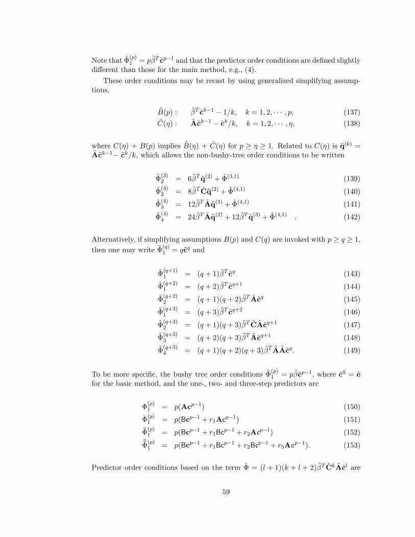
Note that Φ(p)1 = pβT cp−1 and that the predictor order conditions are defined slightly
different than those for the main method, e.g., (4).
These order conditions may be recast by using generalized simplifying assump-tions,
B(p) : βT ck−1 − 1/k, k = 1, 2, · · · , p, (137)
C(η) : Ack−1 − ck/k, k = 1, 2, · · · , η, (138)
where C(η) + B(p) implies B(η) + C(η) for p ≥ η ≥ 1. Related to C(η) is q(k) =Ack−1− ck/k, which allows the non-bushy-tree order conditions to be written
Φ(3)2 = 6βT q(2) + Φ(3,1) (139)
Φ(4)2 = 8βT Cq(2) + Φ(4,1) (140)
Φ(4)3 = 12βT Aq(3) + Φ(4,1) (141)
Φ(4)4 = 24βT Aq(2) + 12βT q(3) + Φ(4,1) . (142)
Alternatively, if simplifying assumptions B(p) and C(q) are invoked with p ≥ q ≥ 1,
then one may write Φ(q)1 = qcq and
Φ(q+1)1 = (q + 1)βT cq (143)
Φ(q+2)1 = (q + 2)βT cq+1 (144)
Φ(q+2)2 = (q + 1)(q + 2)βT Acq (145)
Φ(q+3)1 = (q + 3)βT cq+2 (146)
Φ(q+3)2 = (q + 1)(q + 3)βT CAcq+1 (147)
Φ(q+3)3 = (q + 2)(q + 3)βT Acq+1 (148)
Φ(q+3)4 = (q + 1)(q + 2)(q + 3)βT AAcq. (149)
To be more specific, the bushy tree order conditions Φ(p)1 = pβcp−1, where c0 = e
for the basic method, and the one-, two- and three-step predictors are
Φ(p)1 = p(Acp−1) (150)
Φ(p)1 = p(Bcp−1 + r1Acp−1) (151)
¯Φ(p)1 = p(Bcp−1 + r1Bc
p−1 + r2Acp−1) (152)¯Φ
(p)1 = p(Bcp−1 + r1Bc
p−1 + r2Bcp−1 + r3Acp−1). (153)
Predictor order conditions based on the term Φ = (l + 1)(k + l + 2)βT CkAcl are
59
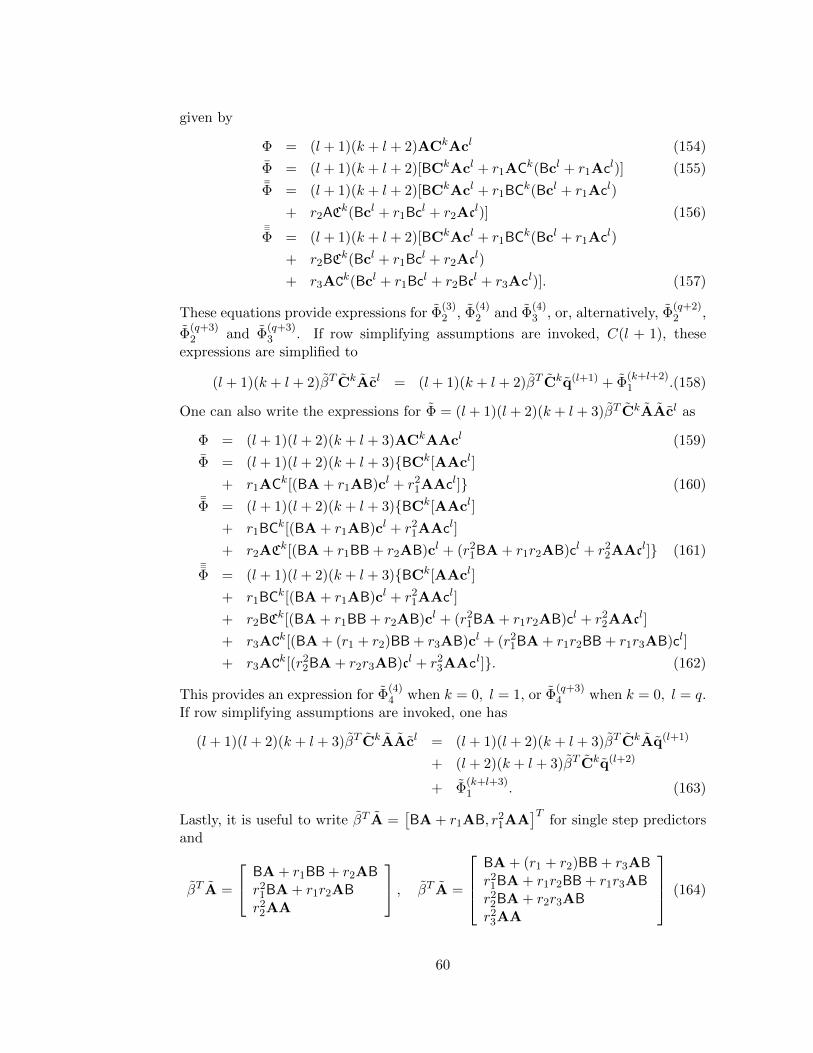
given by
Φ = (l + 1)(k + l + 2)ACkAcl (154)
Φ = (l + 1)(k + l + 2)[BCkAcl + r1ACk(Bcl + r1Acl)] (155)¯Φ = (l + 1)(k + l + 2)[BCkAcl + r1BC
k(Bcl + r1Acl)
+ r2ACk(Bcl + r1Bc
l + r2Acl)] (156)¯Φ = (l + 1)(k + l + 2)[BCkAcl + r1BC
k(Bcl + r1Acl)
+ r2BCk(Bcl + r1Bc
l + r2Acl)
+ r3ACk(Bcl + r1Bcl + r2Bc
l + r3Acl)]. (157)
These equations provide expressions for Φ(3)2 , Φ
(4)2 and Φ
(4)3 , or, alternatively, Φ
(q+2)2 ,
Φ(q+3)2 and Φ
(q+3)3 . If row simplifying assumptions are invoked, C(l + 1), these
expressions are simplified to
(l + 1)(k + l + 2)βT CkAcl = (l + 1)(k + l + 2)βT Ckq(l+1) + Φ(k+l+2)1 .(158)
One can also write the expressions for Φ = (l + 1)(l + 2)(k + l + 3)βT CkAAcl as
Φ = (l + 1)(l + 2)(k + l + 3)ACkAAcl (159)
Φ = (l + 1)(l + 2)(k + l + 3){BCk[AAcl]
+ r1ACk[(BA + r1AB)cl + r21AAcl]} (160)
¯Φ = (l + 1)(l + 2)(k + l + 3){BCk[AAcl]
+ r1BCk[(BA + r1AB)cl + r2
1AAcl]
+ r2ACk[(BA + r1BB + r2AB)cl + (r21BA + r1r2AB)cl + r2
2AAcl]} (161)¯Φ = (l + 1)(l + 2)(k + l + 3){BCk[AAcl]
+ r1BCk[(BA + r1AB)cl + r2
1AAcl]
+ r2BCk[(BA + r1BB + r2AB)cl + (r2
1BA + r1r2AB)cl + r22AAcl]
+ r3ACk[(BA + (r1 + r2)BB + r3AB)cl + (r21BA + r1r2BB + r1r3AB)cl]
+ r3ACk[(r22BA + r2r3AB)cl + r2
3AAcl]}. (162)
This provides an expression for Φ(4)4 when k = 0, l = 1, or Φ
(q+3)4 when k = 0, l = q.
If row simplifying assumptions are invoked, one has
(l + 1)(l + 2)(k + l + 3)βT CkAAcl = (l + 1)(l + 2)(k + l + 3)βT CkAq(l+1)
+ (l + 2)(k + l + 3)βT Ckq(l+2)
+ Φ(k+l+3)1 . (163)
Lastly, it is useful to write βT A =[BA + r1AB, r2
1AA]T
for single step predictorsand
βT A =
BA + r1BB + r2ABr2
1BA + r1r2ABr2
2AA
, βT A =
BA + (r1 + r2)BB + r3ABr2
1BA + r1r2BB + r1r3ABr2
2BA + r2r3ABr2
3AA
(164)
60
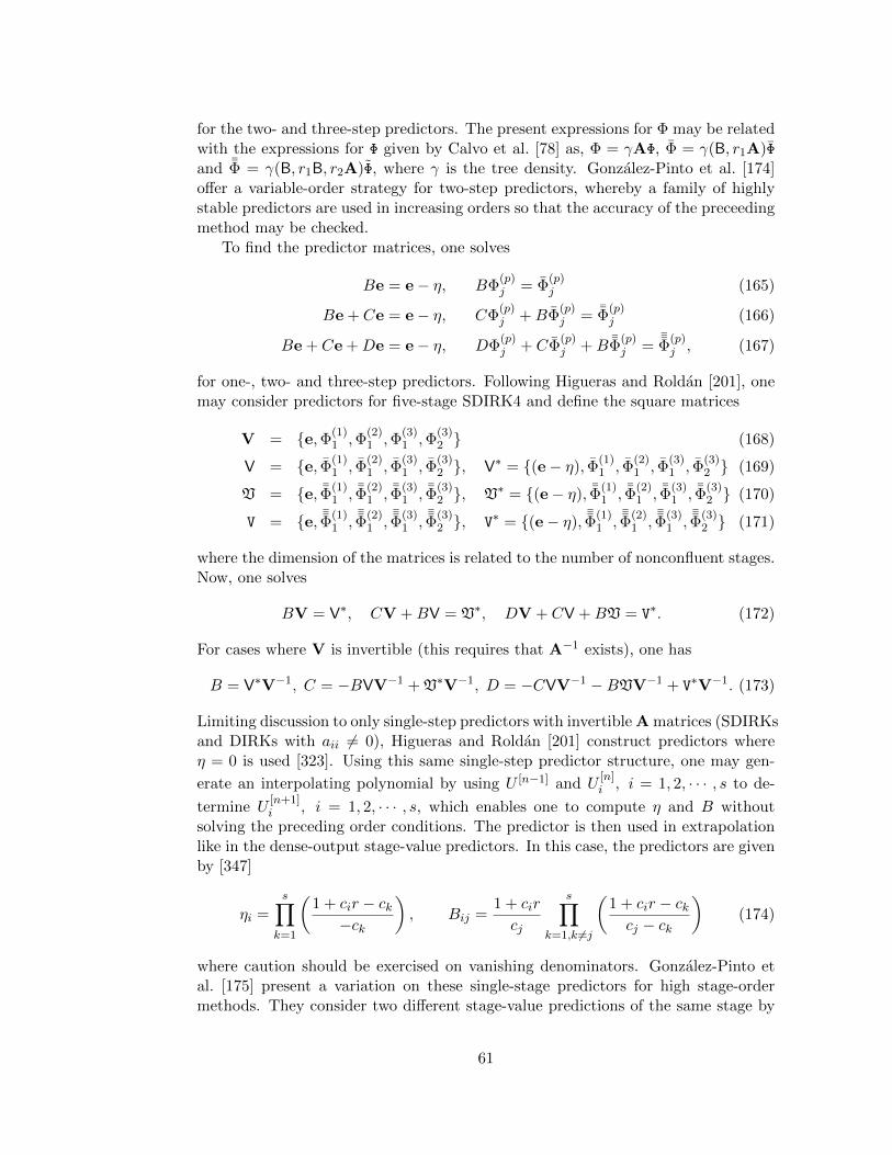
for the two- and three-step predictors. The present expressions for Φ may be relatedwith the expressions for Φ given by Calvo et al. [78] as, Φ = γAΦ, Φ = γ(B, r1A)Φand ¯Φ = γ(B, r1B, r2A)Φ, where γ is the tree density. Gonzalez-Pinto et al. [174]offer a variable-order strategy for two-step predictors, whereby a family of highlystable predictors are used in increasing orders so that the accuracy of the preceedingmethod may be checked.
To find the predictor matrices, one solves
Be = e− η, BΦ(p)j = Φ
(p)j (165)
Be + Ce = e− η, CΦ(p)j +BΦ
(p)j = ¯Φ
(p)j (166)
Be + Ce +De = e− η, DΦ(p)j + CΦ
(p)j +B ¯Φ
(p)j =
¯Φ
(p)j , (167)
for one-, two- and three-step predictors. Following Higueras and Roldan [201], onemay consider predictors for five-stage SDIRK4 and define the square matrices
V = {e,Φ(1)1 ,Φ
(2)1 ,Φ
(3)1 ,Φ
(3)2 } (168)
V = {e, Φ(1)1 , Φ
(2)1 , Φ
(3)1 , Φ
(3)2 }, V∗ = {(e− η), Φ
(1)1 , Φ
(2)1 , Φ
(3)1 , Φ
(3)2 } (169)
V = {e, ¯Φ(1)1 , ¯Φ
(2)1 , ¯Φ
(3)1 , ¯Φ
(3)2 }, V∗ = {(e− η), ¯Φ
(1)1 , ¯Φ
(2)1 , ¯Φ
(3)1 , ¯Φ
(3)2 } (170)
V = {e, ¯Φ
(1)1 ,
¯Φ
(2)1 ,
¯Φ
(3)1 ,
¯Φ
(3)2 }, V∗ = {(e− η),
¯Φ
(1)1 ,
¯Φ
(2)1 ,
¯Φ
(3)1 ,
¯Φ
(3)2 } (171)
where the dimension of the matrices is related to the number of nonconfluent stages.Now, one solves
BV = V∗, CV +BV = V∗, DV + CV +BV = V∗. (172)
For cases where V is invertible (this requires that A−1 exists), one has
B = V∗V−1, C = −BVV−1 + V∗V−1, D = −CVV−1 −BVV−1 + V∗V−1. (173)
Limiting discussion to only single-step predictors with invertible A matrices (SDIRKsand DIRKs with aii 6= 0), Higueras and Roldan [201] construct predictors whereη = 0 is used [323]. Using this same single-step predictor structure, one may gen-
erate an interpolating polynomial by using U [n−1] and U[n]i , i = 1, 2, · · · , s to de-
termine U[n+1]i , i = 1, 2, · · · , s, which enables one to compute η and B without
solving the preceding order conditions. The predictor is then used in extrapolationlike in the dense-output stage-value predictors. In this case, the predictors are givenby [347]
ηi =
s∏k=1
(1 + cir − ck−ck
), Bij =
1 + cir
cj
s∏k=1,k 6=j
(1 + cir − ckcj − ck
)(174)
where caution should be exercised on vanishing denominators. Gonzalez-Pinto etal. [175] present a variation on these single-stage predictors for high stage-ordermethods. They consider two different stage-value predictions of the same stage by
61

using (174) and the analogous formula where ηi = 0. The stage-value predictionis then equal to the latter prediction, plus the product of the inverse iterationmatrix times the difference between the two predicted values in order to introducea stabilizing contribution.
The predictor stability functions at stage i, R(i)pred(z), for (125), (126) and (127)
are then given by [173–175]
R(i)pred(z) = ηi +
s∑j=1
BijR(j)int(z) (175)
R(i)pred(z) = ηi +
s∑j=1
BijR(j)int(r1z)
R(z) +
s∑j=1
CijR(j)int(z) (176)
R(i)pred(z) = ηi +
s∑j=1
BijR(j)int(r2z)
R(r1z)R(z) +
s∑j=1
CijR(j)int(r1z)
R(z)
+s∑j=1
DijR(j)int(z), (177)
where R(j)int(z) is the internal stability function, (53), at stage j. Applied to stiff
problems, R(j)int(−∞) = 0 implies that the starting algorithm cushions the very stiff
components [174]. Three simple things may be done to enhance predictor stability:set ηi = 0, choose an L-stable underlying method, R(−∞) = 0, and design a method
so that R(j)int(−∞) = 0.
When the A-matrix is singular because the first stage is explicit, as it is withEDIRKs, ESDIRKs and QESDIRKs, this single-step structure must be modified[202,204]. Modified stage-value predictors may now be considered in the form
U[n]i+1,0 = ηiU
[n−1] +s−1∑j=1
BijU[n]j+1 (178)
U[n]i+1,0 = ηiU
[n−2] +s−1∑j=1
BijU[n]j+1 +
s−1∑j=1
CijU[n−1]j+1 (179)
U[n]i+1,0 = ηiU
[n−3] +s−1∑j=1
BijU[n]j+1 +
s−1∑j=1
CijU[n−1]j+1 +
s−1∑j=1
DijU[n−2]j+1 , (180)
where i = 1, 2, · · · , (s − 1), the matrices Bij , Cij , and Dij are of dimension (s −1) × (s − 1), and η is a vector of length (s − 1). The conventional Butcher arrayis then decomposed according to (3). Also, b, c and e (composed of ones) arevectors of length (s − 1), and B = e ⊗ b. The components of c are c, c = e + r1c,c = e(1 + r1) + r2c and c = e(1 + r1 + r2) + r3c. Order conditions for these methods
62
are solved by using
Be = e− η, BΦ(p)j = Φ(p)
j (181)
Be + Ce = e− η, CΦ(p)j + B Φ(p)
j =Φ
(p)
j (182)
Be + Ce + De = e− η, DΦ(p)j + C Φ(p)
j + BΦ
(p)
j =Φ
(p)
j . (183)
Higueras and Roldan [202,204] use these relations in the context of single-step predic-tors for ODEs and index-2 DAEs. Order conditions for first-stage explicit methodsare slight modifications of those with invertible A-matrices. The difference termsd = (1 + r1) and d = (1 + r1 + r2) will be useful. Bushy tree order conditions forthe basic method and for one-, two- and three-step predictors are
Φ(p)1 = p(Acp−1) (184)Φ(p)
1 = p(Bcp−1 + r1(Acp−1 + a)) (185)Φ
(p)
1 = p(Bcp−1 + r1Bcp−1 + r2(Acp−1 + adp−1)) (186)
Φ(p)
1 = p(Bcp−1 + r1Bcp−1 + r2Bc
p−1 + r3(Acp−1 + adp−1)). (187)
Order conditions derived from the term Φ = (l + 1)(k + l + 2)βCkAcl are given by
Φ = (l + 1)(k + l + 2)ACkAcl (188)Φ = (l + 1)(k + l + 2)[BCkAcl + r1ACk(Bcl + r1Acl + r1a)] (189)Φ = (l + 1)(k + l + 2)[BCkAcl + r1BC
k(Bcl + r1Acl + r1a)
+ r2ACk(Bcl + r1Bc
l + r2Acl + r2adl)] (190)
Φ = (l + 1)(k + l + 2)[BCkAcl + r1BCk(Bcl + r1Acl + r1a)
+ r2BCk(Bcl + r1Bc
l + r2Acl + r2adl)
+ r3ACk(Bcl + r1Bcl + r2Bc
l + r3Acl + r3adl)]. (191)
Expressions for Φ(3)
2 , Φ(4)
2 and Φ(4)
3 or, alternatively, Φ(q+2)
2 , Φ(q+3)
2 and Φ(q+3)
3 maybe derived by using these relations. One can also write the expressions derived from
63
Φ = (l + 1)(l + 2)(k + l + 3)βCkAAcl as
Φ = (l + 1)(l + 2)(k + l + 3)ACkAAcl (192)Φ = (l + 1)(l + 2)(k + l + 3){BCk[AAcl]
+ r1ACk[(BA + r1AB)cl + r21A(Acl + a)]} (193)
Φ = (l + 1)(l + 2)(k + l + 3){BCk[AAcl]
+ r1BCk[(BA + r1AB)cl + r2
1A(Acl + a)]
+ r2ACk[(BA + r1BB + r2AB)cl + (r21BA + r1r2AB)cl +
r21Ba + r2
2A(Acl + adl)]} (194)Φ = (l + 1)(l + 2)(k + l + 3){BCk[AAcl]
+ r1BCk[(BA + r1AB)cl + r2
1A(Acl + a)]
+ r2BCk[(BA + r1BB + r2AB)cl + (r2
1BA + r1r2AB)cl +
r21Ba + r2
2A(Acl + adl)]
+ r3ACk[(BA + (r1 + r2)BB + r3AB)cl + (r21BA + r1r2BB + r1r3AB)cl +
r21Ba + (r2
2BA + r2r3AB)cl + r22Bad
l + r23A(Acl + adl)]}. (195)
These equations provide an expression for Φ(4,4)
when k = 0, l = 1, or Φ(q+3,4)
whenk = 0, l = q. To solve for the predictor matrices, one may consider a nonconfluentfive-stage, stage-order two ESDIRK and define the square matrices
V = {e, Φ(1)1 , Φ
(2)1 , Φ
(3)1 } (196)
V = {e, Φ(1)
1 , Φ(2)
1 , Φ(3)
1 }, V∗ = {(e− η), Φ(1)
1 , Φ(2)
1 , Φ(3)
1 } (197)
V = {e, Φ(1)
1 ,Φ
(2)
1 ,Φ
(3)
1 }, V∗ = {(e− η),Φ
(1)
1 ,Φ
(2)
1 ,Φ
(3)
1 } (198)
V = {e, Φ(1)
1 ,Φ
(2)
1 ,Φ
(3)
1 }, V∗ = {(e− η),Φ
(1)
1 ,Φ
(2)
1 ,Φ
(3)
1 }, (199)
where the dimension of the matrices is related to the number of nonconfluent stages.Now, one must solve
BV = V∗, CV + BV = V∗, DV + CV + BV = V∗. (200)
In cases where V is invertible (this requires that A−1 exists), one has B = V∗V−1
and
C = −BVV−1 + V∗V−1, D = −CVV−1 − BVV−1 + V∗V−1. (201)
Higueras and Roldan [201] supplement their single-stage predictor, (125), with astrategy described by Hairer and Wanner [193] and used in the SDIRK4 code: theyuse early stage values to predict later stage values. Originally this strategy was based
on the Φ[p]j vectors, but Higueras and Roldan also extend it to include Φ
[p]j vectors.
Before putting these order conditions to use, one may define Z[n]i = U
[n]i − U [n]
64
associated with stage i at t[n] + ci∆t. The starting guess for stage i is then U[n]i,0 =
U [n]+Z[n]i,0 . Hairer and Wanner propose to estimate Z
[n]i,0 by using Z
[n]i,0 =
∑i−1j=1 αjZ
[n]j
where the values αj may be precomputed for each stage. Depending on how manystages of the current step one has completed, one obtains different orders of accuracy.
Considering a five-stage SDIRK such as SDIRK4, Z[n]2 may be computed to first-
order accuracy by using α1 = c2/c1. If the first two (three) stages of an SDIRK
have been computed then Z[n]3 (Z
[n]4 ) may be computed to second-order accuracy by
using (c1 c2
(Ac)1 (Ac)2
)(α1
α2
)=
(c3
(Ac)3
)(202) c1 c2 c3
(Ac)1 (Ac)2 (Ac)3
ϕ(3)1 ϕ
(3)2 ϕ
(3)3
α1
α2
α3
=
c4
(Ac)4
ϕ(3)4
, (203)
where ϕ(3) is some combination of the two third-order trees, Ac2 and A2c. Note
that these terms included are simply proportional to the Φ[p]j given above. On the
fifth-stage, a third-order approximation may be usedc1 c2 c3 c4
(Ac)1 (Ac)2 (Ac)3 (Ac)4(Ac2
)1
(Ac2
)2
(Ac2
)3
(Ac2
)4(
A2c)
1
(A2c
)2
(A2c
)3
(A2c
)4
α1
α2
α3
α4
=
c5
(Ac)5(Ac2
)5(
A2c)
5
. (204)
Hairer and Wanner use dense output for the first stage of SDIRK4, α1 = c2/c1 forstage two, and (202), (203), and (204) for latter stages. Higueras and Roldan [201]found best results for this stage-order one method by using (125) and (165) to predictthe first two stages and (203) and (204) for the fourth- and fifth stages. The thirdstage could be predicted with either (202) or (205) and (206). For EDIRKs, ES-DIRKs and QESDIRKs, one must increase the subscripts by one. If row-simplifyingassumption C(η) is being used, the selection of order conditions must respect po-tentially redundant conditions. This same strategy may also use stage informationfrom the latter stages of the previous step. For instance, to compute
U[n]3 = α1U
[n]3 + α2U
[n]4 + α3U
[n]5 + α4U
[n+1]1 + α5U
[n+1]2 (205)
one solves
1 1 1 1 1c3 c4 c5 c1 c2
(Ac)3 (Ac)4 (Ac)5
(Φ
[2]1
)1
(Φ
[2]1
)2(
Ac2)
3
(Ac2
)4
(Ac2
)5
(Φ
[3]1
)1
(Φ
[3]1
)2(
A2c)
3
(A2c
)4
(A2c
)5
(Φ
[3]2
)1
(Φ
[3]2
)2
α1
α2
α3
α4
α5
=
1c3(
Φ[2]1
)3(
Φ[3]1
)3(
Φ[3]2
)3
.(206)
Notice that when stages from two steps are involved, the summation is over U[n]i and
U[n]i rather than Z
[n]i . This strategy may be extended to include additional prior
steps by using order conditions based on two- and three-step predictors.
65
2.19 Discontinuities
In the course of integrating the ODE
dU
dt= F (U(t), t) (207)
the RHS function, F (U(t), t), or one of its elementary differentials may become dis-continuous [81,96,138,142,166,297,325,380,427]. Examples of situations where thismay occur include the time-dependent temperature in a room when a thermostat isemployed or the time dependent velocity of an object which collides with another ob-ject. In computer codes used to solve time-dependent partial differential equations,temporal discontinuities may arise by changes in boundary conditions or changeswithin a submodel caused by conditional statements. If Runge-Kutta methods at-tempt to integrate over this discontinuity, both local and global errors will likelyincrease unless proper care is taken by the algorithm. A function F (U(t), t) has adiscontinuity of order q − 1 if at least one of the partial derivatives with respect totime is discontinuous of order q − 1, but all partial derivatives with respect to timeof order < q − 1 are continuous. Let FL(U(t), t) and FR(U(t), t) be the functionsto the left and right, respectively, of the discontinuity and let a discontinuity belocated at td. The size of the qth-order discontinuity is given by
d(q−1)FLdt(q−1)
∣∣∣t+d
− d(q−1)FRdt(q−1)
∣∣∣t+d
= Kq, (208)
where the functions are evaluated immediately to the right of the discontinuity,t+d . Only bounded discontinuities will be considered, i.e., Kq is finite. If at somevalue of t = ts, F (U(t), t) becomes infinite, then a singularity has been encountered.Discussions of singular initial value problems may be found in the literature [127,147,249,260,261,418].
Some discontinuities may be anticipated while others may not. Those that areanticipated are often accompanied by switching functions, g(U(t), t). This function,g(U(t), t) = 0, defines the discontinuity hypersurface. Shampine and Thompson[380] consider well-posedness in this situation. If the integration is well-posed onthe interval [a, td] with U(a) = A, then a small perturbation to the initial condition;U(a) = A + α will give rise to a small perturbation in UL(t) by the amount δUL.This then induces a small change in the location of the discontinuity; δt. Taking thefirst terms of a Taylor series expansion about U(t) and td, where g(U(td), td) = 0,
g(UL(td + δt) + δUL, td + δt) = g(UL(td), td) +∂g
∂U
∣∣∣tdδUL
+
(∂g
∂t
∣∣∣td
+∂g
∂U
∣∣∣td
∂U
∂t
∣∣∣td
)δt+ · · ·
= 0 (209)
Hence,
δt = − ∂g∂U
∣∣∣td
(∂g
∂t
∣∣∣td
+∂g
∂U
∣∣∣td
∂U
∂t
∣∣∣td
)−1
δUL. (210)
66
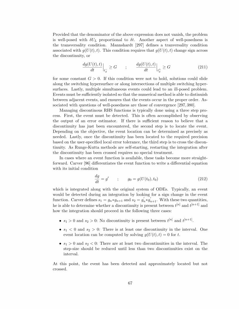
Provided that the denominator of the above expression does not vanish, the problemis well-posed with δUL proportional to δt. Another aspect of well-posedness isthe transversality condition. Mannshardt [297] defines a tranversality conditionassociated with g(U(t), t). This condition requires that g(U(t), t) change sign acrossthe discontinuity, or
dg(U(t), t)
dt
∣∣∣t−d
≥ G ;dg(U(t), t)
dt
∣∣∣t+d
≥ G (211)
for some constant G > 0. If this condition were not to hold, solutions could slidealong the switching hypersurface or along intersections of multiple switching hyper-surfaces. Lastly, multiple simultaneous events could lead to an ill-posed problem.Events must be sufficiently isolated so that the numerical method is able to distinuishbetween adjacent events, and ensures that the events occur in the proper order. As-sociated with questions of well-posedness are those of convergence [297,380].
Managing discontinous RHS functions is typically done using a three step pro-cess. First, the event must be detected. This is often accomplished by observingthe output of an error estimator. If there is sufficient reason to believe that adiscontinuity has just been encountered, the second step is to locate the event.Depending on the objective, the event location can be determined as precisely asneeded. Lastly, once the discontinuity has been located to the required precisionbased on the user-specified local error tolerance, the third step is to cross the discon-tinuity. As Runge-Kutta methods are self-starting, restarting the integration afterthe discontinuity has been crossed requires no special treatment.
In cases where an event function is available, these tasks become more straight-forward. Carver [96] differentiates the event function to write a differential equationwith its initial condition
dg
dt= g′ ; g0 = g(U(t0), t0) (212)
which is integrated along with the original system of ODEs. Typically, an eventwould be detected during an integration by looking for a sign change in the eventfunction. Carver defines s1 = gn∗gn+1 and s2 = g
′n∗g
′n+1. With these two quantities,
he is able to determine whether a discontinuity is present between t[n] and t[n+1] andhow the integration should proceed in the following three cases:
• s1 > 0 and s2 > 0: No discontinuity is present between t[n] and t[n+1].
• s1 < 0 and s2 > 0: There is at least one discontinuity in the interval. Oneevent location can be computed by solving g(U(t), t) = 0 for t.
• s1 > 0 and s2 < 0: There are at least two discontinuities in the interval. Thestep-size should be reduced until less than two discontinuities exist on theinterval.
At this point, the event has been detected and approximately located but notcrossed.
67
Event detection, location and crossing often occur in the general situation whereno event function is available. Several general criteria have been presented in theliterature to detect the presence of a discontinuity in the course of integrating first-order ODEs. They share the objectives of being inexpensive and relying on func-tionality already present in the integration algorithm. Regardless of which criterionis chosen, discontinuities having large values of q but small values of Kq may go un-detected. Further, since local error estimates are used in event detection, lax localerror tolerances may also contribute to a discontinuity going undetected. Ratherthan going undetected, caution should be made to ensure that a discontinuity is notconfused with rapidly varying RHS caused by numerical stiffness. If the integrationmethod lacks sufficient stability, discontinuity detection may be routinely activatedby stiffness.
Assume that the integration has successfully stepped from t[n−1] to t[n] and is
now attempting to step from t[n] to t[n+1] using an initial step-size of (∆t)[n]1 . Assume
that the step is rejected by the error controller. A rejected step is typically whenevent detection is initiated. Gear and Østerby [166] recompute a new step-size to
be used on the failed step, (∆t)[n]2 . A discontinuity is suspected if either criterion is
met:
• (GØ1) 2(∆t)[n]2 < (∆t)
[n]1 then a discontinuity is suspected of being in the
interval {t[n], t[n] + (∆t)[n]1 }.
• (GØ2) There are two successive failed steps, i.e., both (∆t)[n]1 and (∆t)
[n]2 result
in failed steps. In this case, a discontinuity is suspected of being in the interval
{t[n], t[n] + (∆t)[n]2 }.
Enright et al. [142] suspect a discontinuity if:
• (E1) After a step from t[n] to t[n+1] has been rejected j-times, it is accepted on
the (j+1)-th attempt with the step-size (∆t)[n]j+1. A new step-size is estimated
from t[n+1] to t[n+2] as (∆t)[n+1]1 . If (∆t)
[n+1]1 ≥ 2(∆t)
[n]j+1, then a discontinuity
is supected of being in the interval {t[n+1], t[n+1] + (∆t)[n]j+1}.
Lastly, Calvo et al. [81] suspect a discontinuity if either:
• Same as GØ1
• In the last three steps, the code has at least two step rejections.
In some cases, event detection should be disabled. Two such cases are immediatelyfollowing the crossing of a discontinuity and at the beginning of the integration whenapproximate (nonequilibrium) initial conditions have been applied.
Event location may be approached in several different ways [81, 142, 166]. Eachof the proposed strategies are quite involved and will not be reviewed here. Thesepapers discuss how the discontinuity is located to an accuracy sufficient to preservethe local error tolerance prescribed for the integration when the event is crossed.Once the discontinuity has been crossed and the local error has been preserved, theintegration is simply resumed with the event detection logic deactivated for the firststep after the crossing.
68
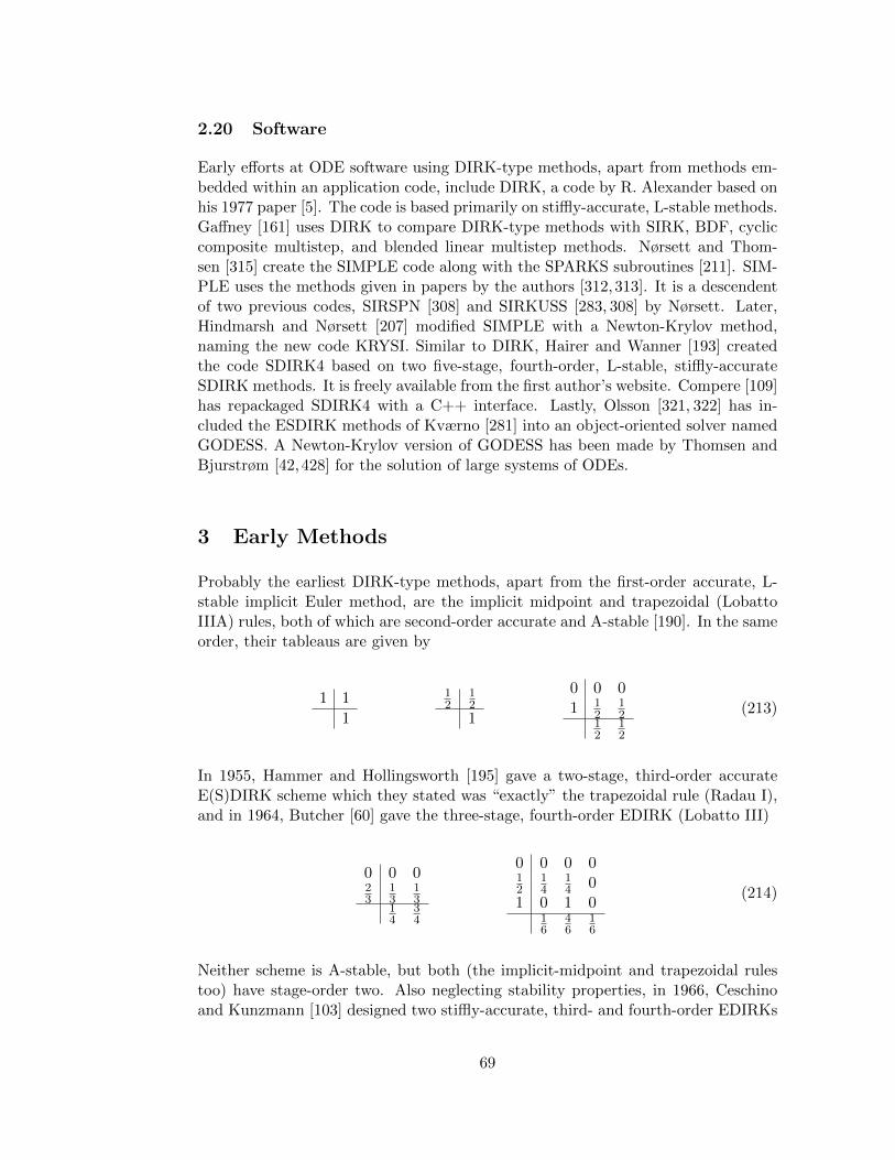
2.20 Software
Early efforts at ODE software using DIRK-type methods, apart from methods em-bedded within an application code, include DIRK, a code by R. Alexander based onhis 1977 paper [5]. The code is based primarily on stiffly-accurate, L-stable methods.Gaffney [161] uses DIRK to compare DIRK-type methods with SIRK, BDF, cycliccomposite multistep, and blended linear multistep methods. Nørsett and Thom-sen [315] create the SIMPLE code along with the SPARKS subroutines [211]. SIM-PLE uses the methods given in papers by the authors [312,313]. It is a descendentof two previous codes, SIRSPN [308] and SIRKUSS [283, 308] by Nørsett. Later,Hindmarsh and Nørsett [207] modified SIMPLE with a Newton-Krylov method,naming the new code KRYSI. Similar to DIRK, Hairer and Wanner [193] createdthe code SDIRK4 based on two five-stage, fourth-order, L-stable, stiffly-accurateSDIRK methods. It is freely available from the first author’s website. Compere [109]has repackaged SDIRK4 with a C++ interface. Lastly, Olsson [321, 322] has in-cluded the ESDIRK methods of Kværno [281] into an object-oriented solver namedGODESS. A Newton-Krylov version of GODESS has been made by Thomsen andBjurstrøm [42,428] for the solution of large systems of ODEs.
3 Early Methods
Probably the earliest DIRK-type methods, apart from the first-order accurate, L-stable implicit Euler method, are the implicit midpoint and trapezoidal (LobattoIIIA) rules, both of which are second-order accurate and A-stable [190]. In the sameorder, their tableaus are given by
1 1
1
12
12
1
0 0 01 1
212
12
12
(213)
In 1955, Hammer and Hollingsworth [195] gave a two-stage, third-order accurateE(S)DIRK scheme which they stated was “exactly” the trapezoidal rule (Radau I),and in 1964, Butcher [60] gave the three-stage, fourth-order EDIRK (Lobatto III)
0 0 023
13
13
14
34
0 0 0 012
14
14 0
1 0 1 016
46
16
(214)
Neither scheme is A-stable, but both (the implicit-midpoint and trapezoidal rulestoo) have stage-order two. Also neglecting stability properties, in 1966, Ceschinoand Kunzmann [103] designed two stiffly-accurate, third- and fourth-order EDIRKs
69
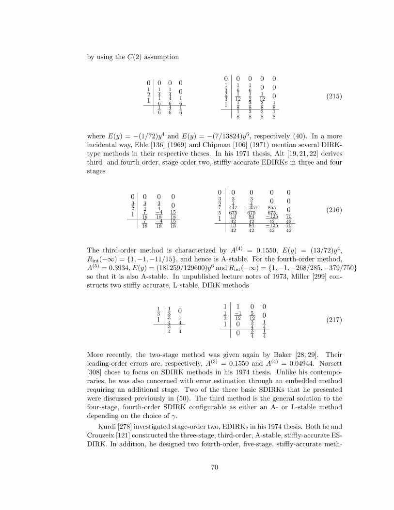
by using the C(2) assumption
0 0 0 012
14
14 0
1 16
46
16
16
46
16
0 0 0 0 013
16
16 0 0
23
112
12
112 0
1 18
38
38
18
18
38
38
18
(215)
where E(y) = −(1/72)y4 and E(y) = −(7/13824)y6, respectively (40). In a moreincidental way, Ehle [136] (1969) and Chipman [106] (1971) mention several DIRK-type methods in their respective theses. In his 1971 thesis, Alt [19, 21, 22] derivesthird- and fourth-order, stage-order two, stiffly-accurate EDIRKs in three and fourstages
0 0 0 032
34
34 0
1 718
−418
1518
718
−418
1518
0 0 0 0 032
34
34 0 0
75
447675
−357675
855675 0
1 1342
8442
−12542
7042
1342
8442
−12542
7042
(216)
The third-order method is characterized by A(4) = 0.1550, E(y) = (13/72)y4,Rint(−∞) = {1,−1,−11/15}, and hence is A-stable. For the fourth-order method,A(5) = 0.3934, E(y) = (181259/129600)y6 andRint(−∞) = {1,−1,−268/285,−379/750}so that it is also A-stable. In unpublished lecture notes of 1973, Miller [299] con-structs two stiffly-accurate, L-stable, DIRK methods
13
13 0
1 34
14
34
14
1 1 0 013−112
512 0
1 0 34
14
0 34
14
(217)
More recently, the two-stage method was given again by Baker [28, 29]. Theirleading-order errors are, respectively, A(3) = 0.1550 and A(4) = 0.04944. Nørsett[308] chose to focus on SDIRK methods in his 1974 thesis. Unlike his contempo-raries, he was also concerned with error estimation through an embedded methodrequiring an additional stage. Two of the three basic SDIRKs that he presentedwere discussed previously in (50). The third method is the general solution to thefour-stage, fourth-order SDIRK configurable as either an A- or L-stable methoddepending on the choice of γ.
Kurdi [278] investigated stage-order two, EDIRKs in his 1974 thesis. Both he andCrouzeix [121] constructed the three-stage, third-order, A-stable, stiffly-accurate ES-DIRK. In addition, he designed two fourth-order, five-stage, stiffly-accurate meth-
70
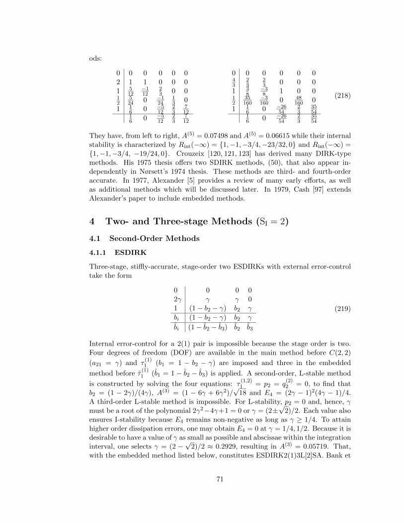
ods:
0 0 0 0 0 02 1 1 0 0 01 5
12−112
23 0 0
12
524 0 −1
2413 0
1 16 0 −5
1223
712
16 0 −5
1223
712
0 0 0 0 0 043
23
23 0 0 0
1 38
−38 1 0 0
12
35160
−3160 0 48
160 01 1
6 0 −2654
23
3554
16 0 −26
5423
3554
(218)
They have, from left to right, A(5) = 0.07498 and A(5) = 0.06615 while their internalstability is characterized by Rint(−∞) = {1,−1,−3/4,−23/32, 0} and Rint(−∞) ={1,−1,−3/4, −19/24, 0}. Crouzeix [120, 121, 123] has derived many DIRK-typemethods. His 1975 thesis offers two SDIRK methods, (50), that also appear in-dependently in Nørsett’s 1974 thesis. These methods are third- and fourth-orderaccurate. In 1977, Alexander [5] provides a review of many early efforts, as wellas additional methods which will be discussed later. In 1979, Cash [97] extendsAlexander’s paper to include embedded methods.
4 Two- and Three-stage Methods (SI = 2)
4.1 Second-Order Methods
4.1.1 ESDIRK
Three-stage, stiffly-accurate, stage-order two ESDIRKs with external error-controltake the form
0 0 0 02γ γ γ 01 (1− b2 − γ) b2 γ
bi (1− b2 − γ) b2 γ
bi (1− b2 − b3) b2 b3
(219)
Internal error-control for a 2(1) pair is impossible because the stage order is two.Four degrees of freedom (DOF) are available in the main method before C(2, 2)
(a21 = γ) and τ(1)1 (b1 = 1 − b2 − γ) are imposed and three in the embedded
method before τ(1)1 (b1 = 1 − b2 − b3) is applied. A second-order, L-stable method
is constructed by solving the four equations: τ(1,2)1 = p2 = q
(2)2 = 0, to find that
b2 = (1 − 2γ)/(4γ), A(3) = (1 − 6γ + 6γ2)/√
18 and E4 = (2γ − 1)2(4γ − 1)/4.A third-order L-stable method is impossible. For L-stability, p2 = 0 and, hence, γmust be a root of the polynomial 2γ2−4γ+1 = 0 or γ = (2±
√2)/2. Each value also
ensures I-stability because E4 remains non-negative as long as γ ≥ 1/4. To attainhigher order dissipation errors, one may obtain E4 = 0 at γ = 1/4, 1/2. Because it isdesirable to have a value of γ as small as possible and abscissae within the integrationinterval, one selects γ = (2 −
√2)/2 ≈ 0.2929, resulting in A(3) = 0.05719. That,
with the embedded method listed below, constitutes ESDIRK2(1)3L[2]SA. Bank et
71
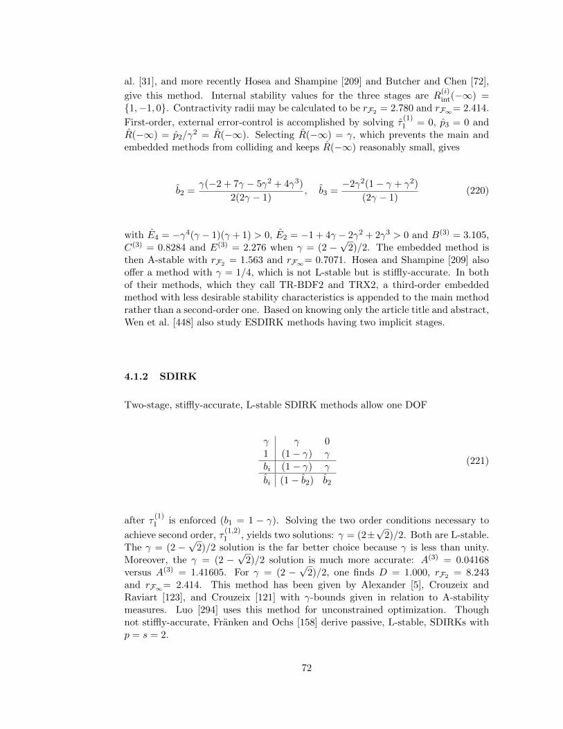
al. [31], and more recently Hosea and Shampine [209] and Butcher and Chen [72],
give this method. Internal stability values for the three stages are R(i)int(−∞) =
{1,−1, 0}. Contractivity radii may be calculated to be rF2 = 2.780 and rF∞= 2.414.
First-order, external error-control is accomplished by solving τ(1)1 = 0, p3 = 0 and
R(−∞) = p2/γ2 = R(−∞). Selecting R(−∞) = γ, which prevents the main and
embedded methods from colliding and keeps R(−∞) reasonably small, gives
b2 =γ(−2 + 7γ − 5γ2 + 4γ3)
2(2γ − 1), b3 =
−2γ2(1− γ + γ2)
(2γ − 1)(220)
with E4 = −γ4(γ − 1)(γ + 1) > 0, E2 = −1 + 4γ − 2γ2 + 2γ3 > 0 and B(3) = 3.105,C(3) = 0.8284 and E(3) = 2.276 when γ = (2 −
√2)/2. The embedded method is
then A-stable with rF2 = 1.563 and rF∞= 0.7071. Hosea and Shampine [209] alsooffer a method with γ = 1/4, which is not L-stable but is stiffly-accurate. In bothof their methods, which they call TR-BDF2 and TRX2, a third-order embeddedmethod with less desirable stability characteristics is appended to the main methodrather than a second-order one. Based on knowing only the article title and abstract,Wen et al. [448] also study ESDIRK methods having two implicit stages.
4.1.2 SDIRK
Two-stage, stiffly-accurate, L-stable SDIRK methods allow one DOF
γ γ 01 (1− γ) γ
bi (1− γ) γ
bi (1− b2) b2
(221)
after τ(1)1 is enforced (b1 = 1 − γ). Solving the two order conditions necessary to
achieve second order, τ(1,2)1 , yields two solutions: γ = (2±
√2)/2. Both are L-stable.
The γ = (2 −√
2)/2 solution is the far better choice because γ is less than unity.Moreover, the γ = (2 −
√2)/2 solution is much more accurate: A(3) = 0.04168
versus A(3) = 1.41605. For γ = (2 −√
2)/2, one finds D = 1.000, rF2 = 8.243and rF∞= 2.414. This method has been given by Alexander [5], Crouzeix andRaviart [123], and Crouzeix [121] with γ-bounds given in relation to A-stabilitymeasures. Luo [294] uses this method for unconstrained optimization. Thoughnot stiffly-accurate, Franken and Ochs [158] derive passive, L-stable, SDIRKs withp = s = 2.
72
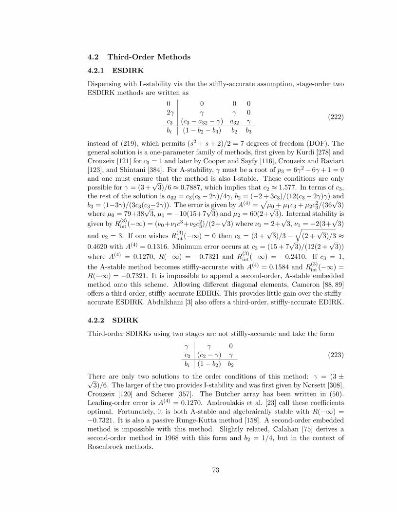
4.2 Third-Order Methods
4.2.1 ESDIRK
Dispensing with L-stability via the the stiffly-accurate assumption, stage-order twoESDIRK methods are written as
0 0 0 02γ γ γ 0c3 (c3 − a32 − γ) a32 γ
bi (1− b2 − b3) b2 b3
(222)
instead of (219), which permits (s2 + s+ 2)/2 = 7 degrees of freedom (DOF). Thegeneral solution is a one-parameter family of methods, first given by Kurdi [278] andCrouzeix [121] for c3 = 1 and later by Cooper and Sayfy [116], Crouzeix and Raviart[123], and Shintani [384]. For A-stability, γ must be a root of p3 = 6γ2− 6γ+ 1 = 0and one must ensure that the method is also I-stable. These conditions are onlypossible for γ = (3 +
√3)/6 ≈ 0.7887, which implies that c2 ≈ 1.577. In terms of c3,
the rest of the solution is a32 = c3(c3 − 2γ)/4γ, b2 = (−2 + 3c3)/(12(c3 − 2γ)γ) andb3 = (1−3γ)/(3c3(c3−2γ)). The error is given by A(4) =
√µ0 + µ1c3 + µ2c2
3/(36√
3)where µ0 = 79+38
√3, µ1 = −10(15+7
√3) and µ2 = 60(2+
√3). Internal stability is
given by R(3)int (−∞) = (ν0+ν1c
3+ν2c23)/(2+
√3) where ν0 = 2+
√3, ν1 = −2(3+
√3)
and ν2 = 3. If one wishes R(3)int (−∞) = 0 then c3 = (3 +
√3)/3 −
√(2 +
√3)/3 ≈
0.4620 with A(4) = 0.1316. Minimum error occurs at c3 = (15 + 7√
3)/(12(2 +√
3))
where A(4) = 0.1270, R(−∞) = −0.7321 and R(3)int (−∞) = −0.2410. If c3 = 1,
the A-stable method becomes stiffly-accurate with A(4) = 0.1584 and R(3)int (−∞) =
R(−∞) = −0.7321. It is impossible to append a second-order, A-stable embeddedmethod onto this scheme. Allowing different diagonal elements, Cameron [88, 89]offers a third-order, stiffly-accurate EDIRK. This provides little gain over the stiffly-accurate ESDIRK. Abdalkhani [3] also offers a third-order, stiffly-accurate EDIRK.
4.2.2 SDIRK
Third-order SDIRKs using two stages are not stiffly-accurate and take the form
γ γ 0c2 (c2 − γ) γ
bi (1− b2) b2
(223)
There are only two solutions to the order conditions of this method: γ = (3 ±√3)/6. The larger of the two provides I-stability and was first given by Nørsett [308],
Crouzeix [120] and Scherer [357]. The Butcher array has been written in (50).Leading-order error is A(4) = 0.1270. Androulakis et al. [23] call these coefficientsoptimal. Fortunately, it is both A-stable and algebraically stable with R(−∞) =−0.7321. It is also a passive Runge-Kutta method [158]. A second-order embeddedmethod is impossible with this method. Slightly related, Calahan [75] derives asecond-order method in 1968 with this form and b2 = 1/4, but in the context ofRosenbrock methods.
73
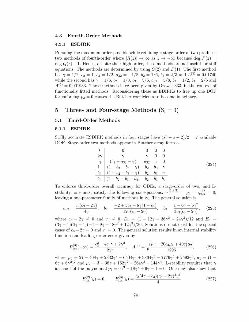
4.3 Fourth-Order Methods
4.3.1 ESDIRK
Pursuing the maximum order possible while retaining a stage-order of two producestwo methods of fourth-order where |R(z)| → ∞ as z → −∞ because deg P (z) =deg Q(z) + 1. Hence, despite their high-order, these methods are not useful for stiffequations. The methods are determined by using C(2) and D(1). The first methodhas γ = 1/2, c2 = 1, c3 = 1/2, a32 = −1/8, b2 = 1/6, b3 = 2/3 and A(5) = 0.01740while the second has γ = 1/6, c2 = 1/3, c3 = 5/6, a32 = 5/8, b2 = 1/2, b3 = 2/5 andA(5) = 0.001933. These methods have been given by Ozawa [333] in the context offunctionally fitted methods. Reconsidering these as EDIRKs to free up one DOFfor enforcing p3 = 0 causes the Butcher coefficients to become imaginary.
5 Three- and Four-stage Methods (SI = 3)
5.1 Third-Order Methods
5.1.1 ESDIRK
Stiffly accurate ESDIRK methods in four stages have (s2 − s + 2)/2 = 7 availableDOF. Stage-order two methods appear in Butcher array form as
0 0 0 0 02γ γ γ 0 0c3 (c3 − a32 − γ) a32 γ 01 (1− b2 − b3 − γ) b2 b3 γ
bi (1− b2 − b3 − γ) b2 b3 γ
bi (1− b2 − b3 − b4) b2 b3 b4
(224)
To enforce third-order overall accuracy for ODEs, a stage-order of two, and L-
stability, one must satisfy the following six equations: τ(1,2,3)1 = p3 = q
(2)2,3 = 0,
leaving a one-parameter family of methods in c3. The general solution is
a32 =c3(c3 − 2γ)
4γ, b2 =
−2 + 3c3 + 6γ(1− c3)
12γ(c3 − 2γ), b3 =
1− 6γ + 6γ2
3c3(c3 − 2γ), (225)
where c3 − 2γ 6= 0 and c3 6= 0, E4 = (1 − 12γ + 36γ2 − 24γ3)/12 and E6 =(3γ − 1)(6γ − 1)(−1 + 9γ − 18γ2 + 12γ3)/36. Solutions do not exist for the specialcases of c3− 2γ = 0 and c3 = 0. The general solution results in an internal stabilityfunction and leading-order error given by
R(3)int (−∞) =
c23 − 4c3γ + 2γ2
2γ2, A(4) =
√µ0 − 20c3µ1 + 40c2
3µ2
1296, (226)
where µ0 = 27 − 408γ + 2332γ2 − 6504γ3 + 9864γ4 − 7776γ5 + 2592γ6, µ1 = (1 −6γ + 6γ2)2 and µ2 = 3 − 38γ + 162γ2 − 264γ3 + 144γ4. L-stability requires that γis a root of the polynomial p3 = 6γ3 − 18γ2 + 9γ − 1 = 0. One may also show that
E(2)int (y) = 0, E
(3)int (y) =
c3(4γ − c3)(c3 − 2γ)2y4
4(227)
74
so that internal I-stability is achieved on stage 3 for c3 ≥ 0 and 4γ ≥ c3. DemandingI-stability of the step requires that E4, E6 > 0 and precludes two of the roots, leavingγ = 0.43586652150845899941601945. This implies that for γ ≈ 0.4358 and 0 ≤ c3 ≤1.743, the third stage is I-stable. This basic scheme has been considered by manyresearchers [7, 8, 88, 89, 281, 396, 398, 426, 450, 451], though probably first by Cooperand Sayfy [116] and later by Alexander and Coyle [8] in the context of DAEs with γ ≈0.4039. One may optimize methods by using c3. Minimum A(4) = 0.03662 occurs at∂A(4)
∂c3= 0 where c3 = (3− 20γ + 24γ2)/(4− 24γ + 24γ2) and R
(3)int (−∞) = −0.8183.
In constructing an IMEX method, Kennedy and Carpenter [255] select the nearby
point c3 = 3/5, where A(4) = 0.03663 and R(3)int (−∞) = −0.8057. Maintaining stiff
accuracy, Skvortsov [398] accepts L(α)-stability (α = 75.6) degrees with the goal toreduce A(4) with his method ES33b.
One may also elect to increase an element of the stage-order vector, taking it from{3,2,2,3} to {3,2,3,3} by selecting c3 = (3±
√3)γ. To keep c3 less than unity, one se-
lects c3 = (3−√
3)γ to find A(4) = 0.03693 and R(3)int (−∞) = −0.7321. Internal error-
control via an A- or L-stable, internal, three-stage, second-order method requiresthat c3 = 1 and E4 = (2γ− 1)2(4γ− 1)/4 ≥ 0. Hence, γ ≥ 1/4 for A-stability of theinternally embedded method and, from before, γ = (2±
√2)/2 for L-stability. The
embedded method is therefore A-stable but not L-stable. This scheme has been givenby Kværno [281, 282] and will be called ESDIRK3(2I)4L[2]SA. Error and stability
are given by A(4) = 0.04907, R(−∞) = R(3)int (−∞) = (2γ2− 4γ+ 1)/2γ2 ≈ −0.9567,
A(3) = 0.1120, B(4) = 1.476, C(4) = 1.912 and E(4) = 0.4380. Optimal inter-
nal stability is achieved when R(3)int (−∞) = 0 by setting c3 = γ(2 ±
√2). Keep-
ing the abscissa within the current step, the c3 = γ(2 −√
2) solution is selectedfor A(4) = 0.04705. An alternative approach to internal error-control is given byWilliams et al. [450, 451] and uses the trapezoidal rule, (213), for the first twostages; that is, γ = 1/2. The 3(2) method is A-stable and has A(4) = 0.1058
and R(3)int (−∞) = −0.5. Cameron [89] designs two A-stable 3(2) pairs by using the
third- and fourth-stages for his two solutions. Thomsen [426] elects to forfeit L-stability by setting γ = 5/12 ≈ 0.4167, but achieves a 3(2) pair with Rint(−∞) ={1,−1,−31/49, 17/125} and A(4) = 0.03291. Cameron [88] proposes a method withinternal error-control and γ = 17/50 = 0.34. Skvortsov’s [396] stiffly-accurate 3(2)pair has γ ≈ 0.1590. Reduced storage via a van der Houwen strategy [256] requiresthat a31 = b1, giving the unacceptably large value of c3 ≈ 1.825. Corresponding
error and internal stability values are A(4) = 0.1080 and R(3)int (−∞) = 1.394. Condi-
tional contractivity requires that all bi > 0, a criterion that cannot be met by thissingle-parameter family of methods. Second-order, external error-control is accom-
plished by solving τ(1,2)1 = p4 = 0, R(−∞) = −p3/γ
3 = γ/2. For a A-stability, onehas
75
b2 =c3(−1 + 6γ − 24γ3 + 12γ4 − 6γ5))
4γ(2γ − c3)(1− 6γ + 6γ2)
+(3− 27γ + 68γ2 − 55γ3 + 21γ4 − 6γ5)
2(2γ − c3)(1− 6γ + 6γ2)
b3 =−γ(−2 + 21γ − 68γ2 + 79γ3 − 33γ4 + 12γ5)
c3(c3 − 2γ)(1− 6γ + 6γ2)
b4 =−3γ2(−1 + 4γ − 2γ2 + γ3)
(1− 6γ + 6γ2)
with E4 = (−1 + 12γ − 48γ2 + 72γ3 − 28γ4 + 12γ5)/4 > 0 and E6 = −γ6(γ −2)(γ + 2)/4 > 0. Selecting this embedded method, L-stability and c3 = 3/5, onemay derive ESDIRK3(2)4L[2]SA where stage 3 is strongly A-stable [255]. The em-bedded method is characterized by A(3) = 0.02552, B(4) = 2.907, C(4) = 1.641 andE(4) = 1.435. If c3 = 1, one may compare the nonstiffly-accurate, stage-order oneexternal value, U (n+1), with the stiffly-accurate, stage-order two internal value ofU (n+1). This comparison may provide some measure of the stiffness. In this case,ESDIRK3(2I)4L[2]SA, one has B(4) = 3.831, C(4) = 1.912 and E(4) = 1.923 for theexternally embedded method. Alexander [7] compares a 3(2) with a 3(4) methodand finds that, due to the conservative nature of the error estimate of the 3(2) pair,the 3(4) pair is more efficient in practice.
5.1.2 QESDIRK
One can use a stiffly-accurate QESDIRK, rather than an ESDIRK, by solving vir-tually the identical order conditions as the increased SOV method but try to mimic
stage-order three behavior at relatively lax tolerances by reducing the error in q(3)2
with SOV = {3, 2, 3, 3}. As the previous ESDIRK has the unpleasantly large valueof c2 ≈ 0.8717, this QESDIRK method provides an opportunity to investigate theutility of differing nonzero diagonal elements [227]. The Butcher array for such amethod is
0 0 0 0 0c2 c2/2 c2/2 0 0c3 (c3 − a32 − γ) a32 γ 01 (1− b2 − b3 − γ) b2 b3 γ
bi (1− b2 − b3 − γ) b2 b3 γ
bi (1− b2 − b3 − b4) b2 b3 b4
(228)
If c2 = 2γ, then the ESDIRK is retrieved. Table 9 lists three possible L-stable QES-DIRKs for the smaller of the two roots giving c3. Only the case where c2 = γ seemsworthy of any further consideration; hence, we give the two nontrivial abscissae:c2 = 4266051685502/7784516477473 and c3 = 3420827508294/7669858543565.
76
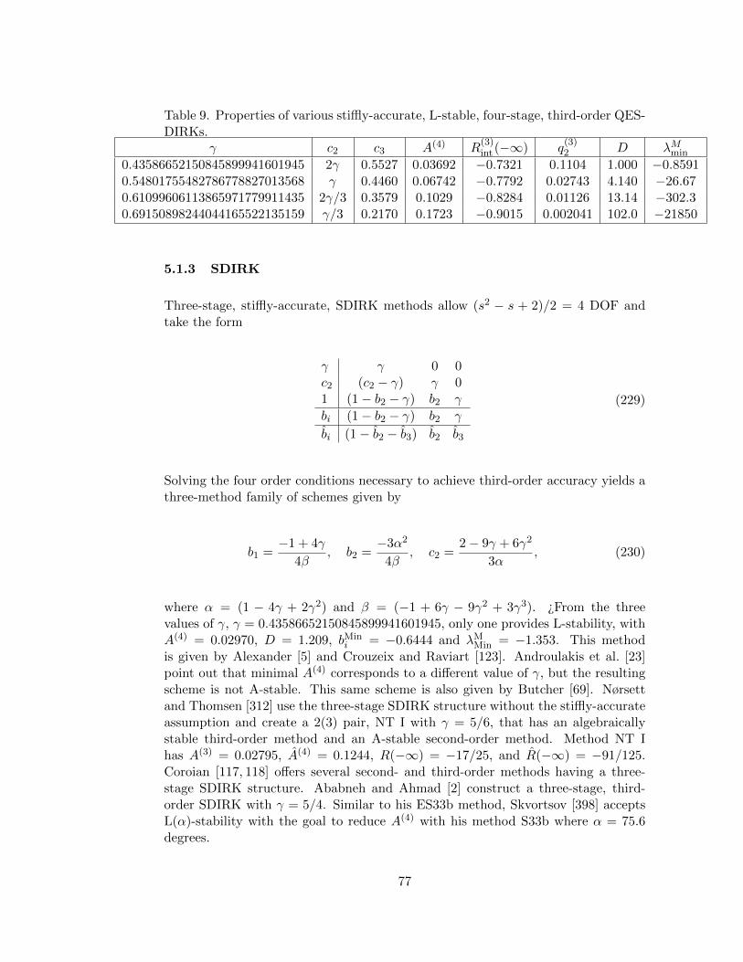
Table 9. Properties of various stiffly-accurate, L-stable, four-stage, third-order QES-DIRKs.
γ c2 c3 A(4) R(3)int (−∞) q
(3)2 D λMmin
0.43586652150845899941601945 2γ 0.5527 0.03692 −0.7321 0.1104 1.000 −0.85910.54801755482786778827013568 γ 0.4460 0.06742 −0.7792 0.02743 4.140 −26.670.61099606113865971779911435 2γ/3 0.3579 0.1029 −0.8284 0.01126 13.14 −302.30.69150898244044165522135159 γ/3 0.2170 0.1723 −0.9015 0.002041 102.0 −21850
5.1.3 SDIRK
Three-stage, stiffly-accurate, SDIRK methods allow (s2 − s + 2)/2 = 4 DOF andtake the form
γ γ 0 0c2 (c2 − γ) γ 01 (1− b2 − γ) b2 γ
bi (1− b2 − γ) b2 γ
bi (1− b2 − b3) b2 b3
(229)
Solving the four order conditions necessary to achieve third-order accuracy yields athree-method family of schemes given by
b1 =−1 + 4γ
4β, b2 =
−3α2
4β, c2 =
2− 9γ + 6γ2
3α, (230)
where α = (1 − 4γ + 2γ2) and β = (−1 + 6γ − 9γ2 + 3γ3). ¿From the threevalues of γ, γ = 0.43586652150845899941601945, only one provides L-stability, withA(4) = 0.02970, D = 1.209, bMin
i = −0.6444 and λMMin = −1.353. This method
is given by Alexander [5] and Crouzeix and Raviart [123]. Androulakis et al. [23]point out that minimal A(4) corresponds to a different value of γ, but the resultingscheme is not A-stable. This same scheme is also given by Butcher [69]. Nørsettand Thomsen [312] use the three-stage SDIRK structure without the stiffly-accurateassumption and create a 2(3) pair, NT I with γ = 5/6, that has an algebraicallystable third-order method and an A-stable second-order method. Method NT Ihas A(3) = 0.02795, A(4) = 0.1244, R(−∞) = −17/25, and R(−∞) = −91/125.Coroian [117, 118] offers several second- and third-order methods having a three-stage SDIRK structure. Ababneh and Ahmad [2] construct a three-stage, third-order SDIRK with γ = 5/4. Similar to his ES33b method, Skvortsov [398] acceptsL(α)-stability with the goal to reduce A(4) with his method S33b where α = 75.6degrees.
77
5.2 Fourth-Order Methods
5.2.1 ESDIRK
Stage-order two, fourth-order ESDIRK methods in four stages
0 0 0 0 02γ γ γ 0 0c3 (c3 − a32 − γ) a32 γ 0c4 (c4 − a42 − a43 − γ) a42 a43 γ
bi (1− b2 − b3 − γ) b2 b3 b4
(231)
that are at least A-stable constitute a two-parameter family of non-stiffly-accurate
methods in, e.g., c3 and c4 where one must solve τ(1,2,3,4)1 = p4 = q
(2)2,3,4 = τ
(4)3 =
0. Solving p4 = (1 − 12γ + 36γ2 − 24γ3) = 0 and requiring I-stability givesγ =
(3 + 2
√3 cos
(π18
))/6 ≈ 1.069. Taking the derivatives of A(5) with respect
to c3 and c4, the minimum error occurs in the immediate vicinity of c3 = 5/7and c4 = 4/7, but the error is still a rather unimpressive A(5) = 0.2328. At thissame point, Rint(−∞) = {1,−1,−0.1135,−0.3543}, R(−∞) = −0.6304, b > 0 andthe four eigenvalues of M are {1.353,−0.06234, 0.02493,−0.003735}. Cooper andSayfy [116], Crouzeix and Raviart [123] and Shintani [384] also derive methods ofthis class.
5.2.2 SDIRK
The three-stage, fourth-order, SDIRK family of methods
γ γ 0 0c2 (c2 − γ) γ 0c3 (c3 − a32 − a32) a32 γ
bi (1− b2 − b3) b2 b3
(232)
has three members, only one of which is A-stable; γ =(3 + 2
√3 cos
(π18
))/6 ≈ 1.069.
Both Nørsett [308] and Crouzeix [120] discovered this method, (50), where A(5) =0.2570, R(−∞) = −0.6304, and the eigenvalues of M are {1.553, 0, 0}. It may be
obtained by solving B(4) for b and c2, τ(4)2 = τ
(3)2 = 0 for a32 and c3 and, lastly,
τ(4)4 = 0 for γ. Alternatively, one could use D(1). As stated earlier, the method is
algebraically stable and therefore A-stable as well. Franken and Ochs [158] constructa passive DIRK analog of this class of methods along with an L-stable version thatis third-order.
5.3 Fifth-Order Methods
5.3.1 ESDIRK
Al-Rabeh [18] has designed fifth-order ESDIRK methods in four-stages by usingassumptions C(2), D(1) and the structure given in (231). Unfortunately, deg P (z)= 1 + deg Q(z), making the methods highly inappropriate for stiff problems. Three
78
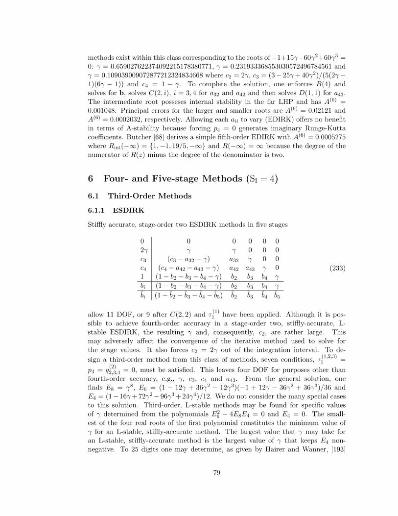
methods exist within this class corresponding to the roots of −1+15γ−60γ2+60γ3 =0: γ = 0.659027622374092215178380771, γ = 0.231933368553030572496784561 andγ = 0.109039009072877212324834668 where c2 = 2γ, c3 = (3− 25γ+ 40γ2)/(5(2γ−1)(6γ − 1)) and c4 = 1 − γ. To complete the solution, one enforces B(4) andsolves for b, solves C(2, i), i = 3, 4 for a32 and a42 and then solves D(1, 1) for a43.The intermediate root posseses internal stability in the far LHP and has A(6) =0.001048. Principal errors for the larger and smaller roots are A(6) = 0.02121 andA(6) = 0.0002032, respectively. Allowing each aii to vary (EDIRK) offers no benefitin terms of A-stability because forcing p4 = 0 generates imaginary Runge-Kuttacoefficients. Butcher [68] derives a simple fifth-order EDIRK with A(6) = 0.0005275where Rint(−∞) = {1,−1, 19/5,−∞} and R(−∞) = ∞ because the degree of thenumerator of R(z) minus the degree of the denominator is two.
6 Four- and Five-stage Methods (SI = 4)
6.1 Third-Order Methods
6.1.1 ESDIRK
Stiffly accurate, stage-order two ESDIRK methods in five stages
0 0 0 0 0 02γ γ γ 0 0 0c3 (c3 − a32 − γ) a32 γ 0 0c4 (c4 − a42 − a43 − γ) a42 a43 γ 01 (1− b2 − b3 − b4 − γ) b2 b3 b4 γ
bi (1− b2 − b3 − b4 − γ) b2 b3 b4 γ
bi (1− b2 − b3 − b4 − b5) b2 b3 b4 b5
(233)
allow 11 DOF, or 9 after C(2, 2) and τ(1)1 have been applied. Although it is pos-
sible to achieve fourth-order accuracy in a stage-order two, stiffly-accurate, L-stable ESDIRK, the resulting γ and, consequently, c2, are rather large. Thismay adversely affect the convergence of the iterative method used to solve forthe stage values. It also forces c2 = 2γ out of the integration interval. To de-
sign a third-order method from this class of methods, seven conditions, τ(1,2,3)1 =
p4 = q(2)2,3,4 = 0, must be satisfied. This leaves four DOF for purposes other than
fourth-order accuracy, e.g., γ, c3, c4 and a43. From the general solution, onefinds E8 = γ8, E6 = (1 − 12γ + 36γ2 − 12γ3)(−1 + 12γ − 36γ2 + 36γ3)/36 andE4 = (1−16γ+ 72γ2−96γ3 + 24γ4)/12. We do not consider the many special casesto this solution. Third-order, L-stable methods may be found for specific valuesof γ determined from the polynomials E2
6 − 4E8E4 = 0 and E4 = 0. The small-est of the four real roots of the first polynomial constitutes the minimum value ofγ for an L-stable, stiffly-accurate method. The largest value that γ may take foran L-stable, stiffly-accurate method is the largest value of γ that keeps E4 non-negative. To 25 digits one may determine, as given by Hairer and Wanner, [193]
79
0.2236478009341764510696898 ≤ γ ≤ 0.5728160624821348554080014. Internal sta-bility of the third- and fourth-stages are given by
R(3)int (−∞) =
c23 − 4c3γ + 2γ2
2γ2(234)
R(4)int (−∞) =
γ(c24 − 4c4γ + 2γ2)− (a43c3(c3 − 2γ))
2γ3(235)
The first vanishes when c3 = γ(2 ±√
2), and the second vanishes when a43 =γ(c24−4c3γ+2γ2)
c3(c3−2γ) . Several different approaches can lead to useful methods. With exter-nal error-control, one could take advantage of the low truncation error of the secondstage relative to the second stage of the 3(2) from the previous section. Enforcing
q(3)3,4 = 0 and R
(4)int (−∞) = 0, while minimizing γ with γ = 9/40 = 0.225, leads to
three methods with a SOV of {3, 2, 3, 3, 3}, c3 = (3−√
3)γ and R(3)int (−∞) = −0.7321
and three with c3 = (3 +√
3)γ and R(3)int (−∞) = 2.7321. Amongst the solu-
tions using c3 = (3 −√
3)γ, the two better solutions have c4 = 41153159264417972126390072 and
A(4) = 0.01283 and c4 = 110884490577711853057145576 and A(4) = 0.002399. Order conditions for
the externally embedded scheme are τ(1,2)1 = p5 = p4 = 0 and τ
(3)1 = 1/600. In-
stead of maximizing the elements of the stage-order vector, one could choose to
simply have R(3)int (−∞) = R
(4)int (−∞) = 0 and find the solution having the min-
imum A(4). This occurs for γ = 9/40 = 0.225 at c3 = 9(2 +√
2)/40 and ap-proximately c3 = 3/5 where A(4) = 0.0007769; using the embedded method justdescribed, A(3) = 0.002357, B(4) = 1.966, C(4) = 1.095 and E(4) = 2.134. Theactual mimima of the system is A(4) = 0.0007666 at γ = 9/40 where the methodis I-stable on all internal stages and, hence, A-stable on stage 2 and L-stable onstages 3,4 and 5. This scheme, ESDIRK3(2)5L[2]SA, appears in Table 10. Notethat ai1 = ai2, i = 1, 2, . . . , s. Another option is to use L-stable internal error-
control by setting c4 = 1 and R(−∞) = R(4)int (−∞) = 0. The resulting four-stage,
second-order internally embedded method is I-stable only if both E6 = γ6 andE4 = (−1 + 12γ − 48γ2 + 72γ3 − 24γ4)/4 are non-negative. The former simply re-quires γ ≥ 0, while the latter additionally requires 0.1804253064293985641345831 ≤γ ≤ 2.1856000973550400826291400. Hence, the acceptable values of γ for the mainmethod are a subset of those that are acceptable for an L-stable, internally embeddedmethod. By selecting γ = 9/40 = 0.225, both main and internal embedded methods
are L-stable. For the final degree of freedom, c3, enforcing R(3)int (−∞) = 0 gives
c3 = 9(2±√
2)/40 from which one selects c3 = 9(2−√
2)/40 to find A(4) = 0.06446.Relaxing the stability constraint on stage three, one sets c3 = 4/5, which gives a
better method with A(4) = 0.01149 and R(3)int (−∞) = 17/81. As stages 2,3 and 4
are I-stable, stage 2 is strictly A-stable, stage 3 is strongly A-stable and stage 4 isL-stable. Order conditions for the external controller are the same as those given
previously, except the last equation that is changed to τ(3)1 = 1/180. For the in-
ternally embedded method, B(5) = 1.388, C(5) = 1.613 and E(5) = 0.2678. Theexternally embedded method has B(5) = 1.216 and E(5) = 0.4877. The scheme,ESDIRK3(2I)5L[2]SA, is presented in Table 11. If one insists on keeping γ = 9/40,
80
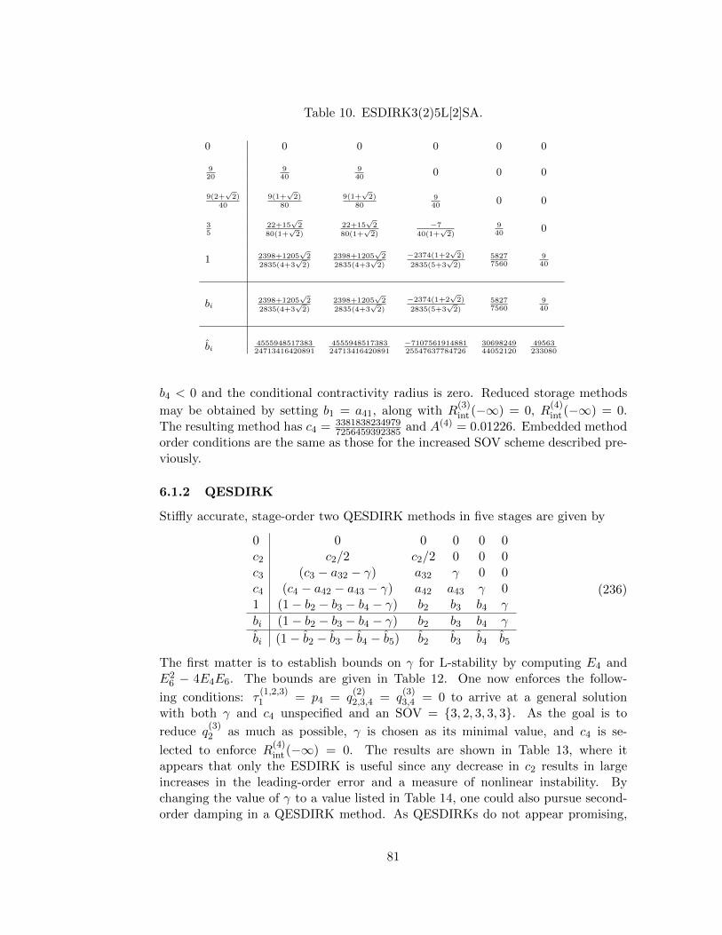
Table 10. ESDIRK3(2)5L[2]SA.
0 0 0 0 0 0
920
940
940
0 0 0
9(2+√2)
409(1+
√2)
809(1+
√2)
80940
0 0
35
22+15√
2
80(1+√2)
22+15√
2
80(1+√2)
−7
40(1+√2)
940
0
1 2398+1205√2
2835(4+3√2)
2398+1205√
2
2835(4+3√2)
−2374(1+2√2)
2835(5+3√2)
58277560
940
bi2398+1205
√2
2835(4+3√2)
2398+1205√
2
2835(4+3√2)
−2374(1+2√2)
2835(5+3√2)
58277560
940
bi455594851738324713416420891
455594851738324713416420891
−710756191488125547637784726
3069824944052120
49563233080
b4 < 0 and the conditional contractivity radius is zero. Reduced storage methods
may be obtained by setting b1 = a41, along with R(3)int (−∞) = 0, R
(4)int (−∞) = 0.
The resulting method has c4 = 33818382349797256459392385 and A(4) = 0.01226. Embedded method
order conditions are the same as those for the increased SOV scheme described pre-viously.
6.1.2 QESDIRK
Stiffly accurate, stage-order two QESDIRK methods in five stages are given by
0 0 0 0 0 0c2 c2/2 c2/2 0 0 0c3 (c3 − a32 − γ) a32 γ 0 0c4 (c4 − a42 − a43 − γ) a42 a43 γ 01 (1− b2 − b3 − b4 − γ) b2 b3 b4 γ
bi (1− b2 − b3 − b4 − γ) b2 b3 b4 γ
bi (1− b2 − b3 − b4 − b5) b2 b3 b4 b5
(236)
The first matter is to establish bounds on γ for L-stability by computing E4 andE2
6 − 4E4E6. The bounds are given in Table 12. One now enforces the follow-
ing conditions: τ(1,2,3)1 = p4 = q
(2)2,3,4 = q
(3)3,4 = 0 to arrive at a general solution
with both γ and c4 unspecified and an SOV = {3, 2, 3, 3, 3}. As the goal is to
reduce q(3)2 as much as possible, γ is chosen as its minimal value, and c4 is se-
lected to enforce R(4)int (−∞) = 0. The results are shown in Table 13, where it
appears that only the ESDIRK is useful since any decrease in c2 results in largeincreases in the leading-order error and a measure of nonlinear instability. Bychanging the value of γ to a value listed in Table 14, one could also pursue second-order damping in a QESDIRK method. As QESDIRKs do not appear promising,
81
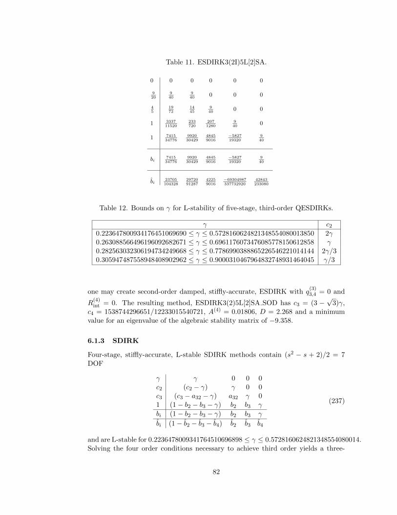
Table 11. ESDIRK3(2I)5L[2]SA.
0 0 0 0 0 0
920
940
940
0 0 0
45
1972
1445
940
0 0
1 333711520
233720
2071280
940
0
1 741534776
992030429
48459016
−582719320
940
bi741534776
992030429
48459016
−582719320
940
bi23705104328
2972091287
42259016
−69304987337732920
42843233080
Table 12. Bounds on γ for L-stability of five-stage, third-order QESDIRKs.
γ c2
0.223647800934176451069690 ≤ γ ≤ 0.5728160624821348554080013850 2γ0.263088566496196092682671 ≤ γ ≤ 0.6961176073476085778150612858 γ0.282563032306194734249668 ≤ γ ≤ 0.7786990388865226546221014144 2γ/30.305947487558948408902962 ≤ γ ≤ 0.9000310467964832748931464045 γ/3
one may create second-order damped, stiffly-accurate, ESDIRK with q(3)3,4 = 0 and
R(4)int = 0. The resulting method, ESDIRK3(2)5L[2]SA SOD has c3 = (3 −
√3)γ,
c4 = 1538744296651/12233015540721, A(4) = 0.01806, D = 2.268 and a minimumvalue for an eigenvalue of the algebraic stability matrix of −9.358.
6.1.3 SDIRK
Four-stage, stiffly-accurate, L-stable SDIRK methods contain (s2 − s + 2)/2 = 7DOF
γ γ 0 0 0c2 (c2 − γ) γ 0 0c3 (c3 − a32 − γ) a32 γ 01 (1− b2 − b3 − γ) b2 b3 γ
bi (1− b2 − b3 − γ) b2 b3 γ
bi (1− b2 − b3 − b4) b2 b3 b4
(237)
and are L-stable for 0.2236478009341764510696898 ≤ γ ≤ 0.5728160624821348554080014.Solving the four order conditions necessary to achieve third order yields a three-
82
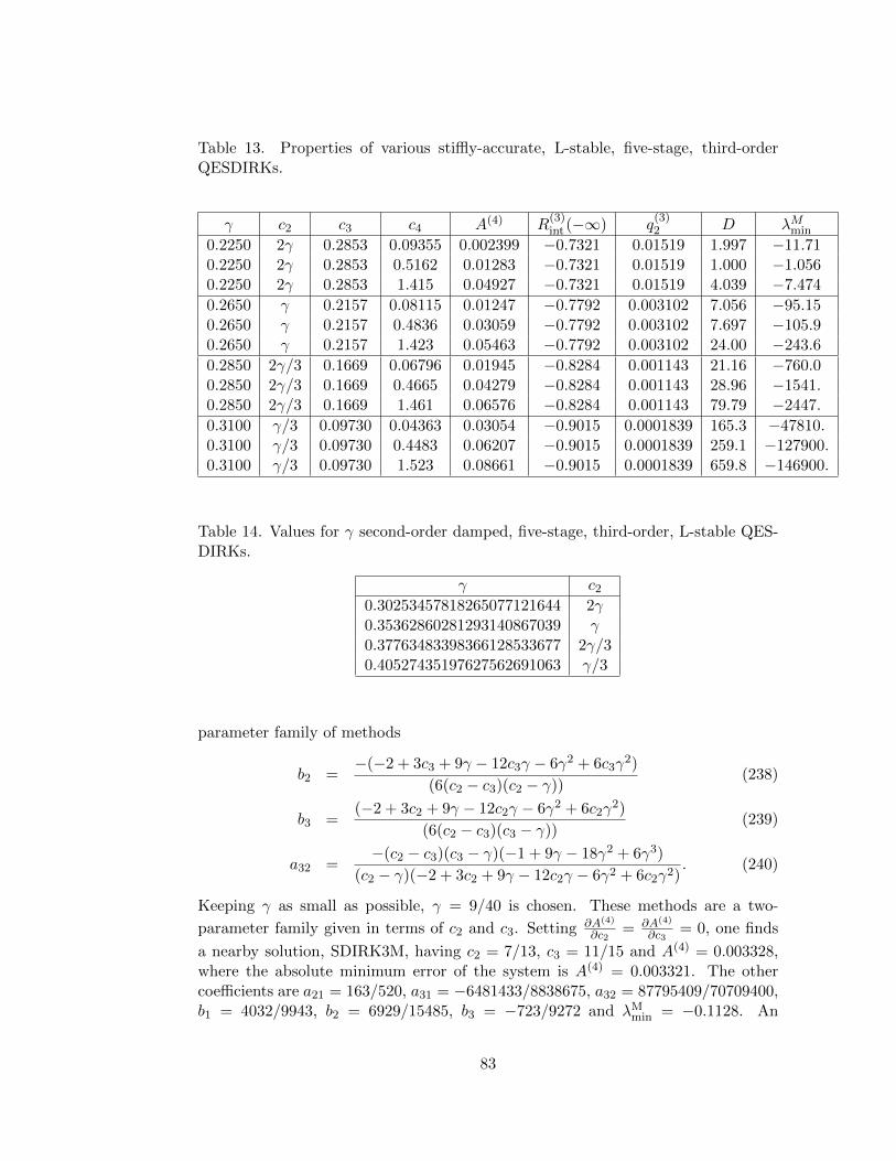
Table 13. Properties of various stiffly-accurate, L-stable, five-stage, third-orderQESDIRKs.
γ c2 c3 c4 A(4) R(3)int (−∞) q
(3)2 D λMmin
0.2250 2γ 0.2853 0.09355 0.002399 −0.7321 0.01519 1.997 −11.710.2250 2γ 0.2853 0.5162 0.01283 −0.7321 0.01519 1.000 −1.0560.2250 2γ 0.2853 1.415 0.04927 −0.7321 0.01519 4.039 −7.474
0.2650 γ 0.2157 0.08115 0.01247 −0.7792 0.003102 7.056 −95.150.2650 γ 0.2157 0.4836 0.03059 −0.7792 0.003102 7.697 −105.90.2650 γ 0.2157 1.423 0.05463 −0.7792 0.003102 24.00 −243.6
0.2850 2γ/3 0.1669 0.06796 0.01945 −0.8284 0.001143 21.16 −760.00.2850 2γ/3 0.1669 0.4665 0.04279 −0.8284 0.001143 28.96 −1541.0.2850 2γ/3 0.1669 1.461 0.06576 −0.8284 0.001143 79.79 −2447.
0.3100 γ/3 0.09730 0.04363 0.03054 −0.9015 0.0001839 165.3 −47810.0.3100 γ/3 0.09730 0.4483 0.06207 −0.9015 0.0001839 259.1 −127900.0.3100 γ/3 0.09730 1.523 0.08661 −0.9015 0.0001839 659.8 −146900.
Table 14. Values for γ second-order damped, five-stage, third-order, L-stable QES-DIRKs.
γ c2
0.30253457818265077121644 2γ0.35362860281293140867039 γ0.37763483398366128533677 2γ/30.40527435197627562691063 γ/3
parameter family of methods
b2 =−(−2 + 3c3 + 9γ − 12c3γ − 6γ2 + 6c3γ
2)
(6(c2 − c3)(c2 − γ))(238)
b3 =(−2 + 3c2 + 9γ − 12c2γ − 6γ2 + 6c2γ
2)
(6(c2 − c3)(c3 − γ))(239)
a32 =−(c2 − c3)(c3 − γ)(−1 + 9γ − 18γ2 + 6γ3)
(c2 − γ)(−2 + 3c2 + 9γ − 12c2γ − 6γ2 + 6c2γ2). (240)
Keeping γ as small as possible, γ = 9/40 is chosen. These methods are a two-
parameter family given in terms of c2 and c3. Setting ∂A(4)
∂c2= ∂A(4)
∂c3= 0, one finds
a nearby solution, SDIRK3M, having c2 = 7/13, c3 = 11/15 and A(4) = 0.003328,where the absolute minimum error of the system is A(4) = 0.003321. The othercoefficients are a21 = 163/520, a31 = −6481433/8838675, a32 = 87795409/70709400,b1 = 4032/9943, b2 = 6929/15485, b3 = −723/9272 and λM
min = −0.1128. An
83
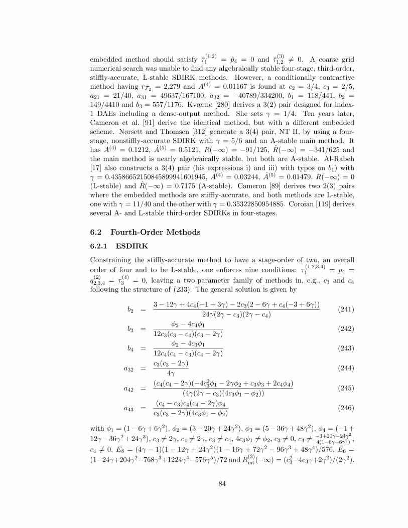
embedded method should satisfy τ(1,2)1 = p4 = 0 and τ
(3)1,2 6= 0. A coarse grid
numerical search was unable to find any algebraically stable four-stage, third-order,stiffly-accurate, L-stable SDIRK methods. However, a conditionally contractivemethod having rF2 = 2.279 and A(4) = 0.01167 is found at c2 = 3/4, c3 = 2/5,a21 = 21/40, a31 = 49637/167100, a32 = −40789/334200, b1 = 118/441, b2 =149/4410 and b3 = 557/1176. Kværnø [280] derives a 3(2) pair designed for index-1 DAEs including a dense-output method. She sets γ = 1/4. Ten years later,Cameron et al. [91] derive the identical method, but with a different embeddedscheme. Nørsett and Thomsen [312] generate a 3(4) pair, NT II, by using a four-stage, nonstiffly-accurate SDIRK with γ = 5/6 and an A-stable main method. Ithas A(4) = 0.1212, A(5) = 0.5121, R(−∞) = −91/125, R(−∞) = −341/625 andthe main method is nearly algebraically stable, but both are A-stable. Al-Rabeh[17] also constructs a 3(4) pair (his expressions i) and iii) with typos on b1) withγ = 0.43586652150845899941601945, A(4) = 0.03244, A(5) = 0.01479, R(−∞) = 0(L-stable) and R(−∞) = 0.7175 (A-stable). Cameron [89] derives two 2(3) pairswhere the embedded methods are stiffly-accurate, and both methods are L-stable,one with γ = 11/40 and the other with γ = 0.35322850954885. Coroian [119] derivesseveral A- and L-stable third-order SDIRKs in four-stages.
6.2 Fourth-Order Methods
6.2.1 ESDIRK
Constraining the stiffly-accurate method to have a stage-order of two, an overall
order of four and to be L-stable, one enforces nine conditions: τ(1,2,3,4)1 = p4 =
q(2)2,3,4 = τ
(4)3 = 0, leaving a two-parameter family of methods in, e.g., c3 and c4
following the structure of (233). The general solution is given by
b2 =3− 12γ + 4c4(−1 + 3γ)− 2c3(2− 6γ + c4(−3 + 6γ))
24γ(2γ − c3)(2γ − c4)(241)
b3 =φ2 − 4c4φ1
12c3(c3 − c4)(c3 − 2γ)(242)
b4 =φ2 − 4c3φ1
12c4(c4 − c3)(c4 − 2γ)(243)
a32 =c3(c3 − 2γ)
4γ(244)
a42 =(c4(c4 − 2γ)(−4c2
3φ1 − 2γφ2 + c3φ3 + 2c4φ4)
(4γ(2γ − c3)(4c3φ1 − φ2))(245)
a43 =(c4 − c3)c4(c4 − 2γ)φ4
c3(c3 − 2γ)(4c3φ1 − φ2)(246)
with φ1 = (1− 6γ+ 6γ2), φ2 = (3− 20γ+ 24γ2), φ3 = (5− 36γ+ 48γ2), φ4 = (−1 +
12γ−36γ2 +24γ3), c3 6= 2γ, c4 6= 2γ, c3 6= c4, 4c3φ1 6= φ2, c3 6= 0, c4 6= −3+20γ−24γ2
4(1−6γ+6γ2),
c4 6= 0, E8 = (4γ − 1)(1 − 12γ + 24γ2)(1 − 16γ + 72γ2 − 96γ3 + 48γ4)/576, E6 =
(1−24γ+204γ2−768γ3+1224γ4−576γ5)/72 andR(3)int (−∞) = (c2
3−4c3γ+2γ2)/(2γ2).
84
No attempt is made to consider all special cases of this general solution becausespecial cases rarely prove to be the most useful methods. Solving p4 = 0 con-strains γ to be a root of the polynomial 1 − 16γ + 72γ2 − 96γ3 + 24γ4, but I-stability requires that both E6 and E8 be non-negative. Of the four roots top4 = 0, only γ ≈ 0.5728160624821348554080014 satifies all three criteria. Min-imum A(5) for this two free-parameter family of methods may be determined by
taking ∂A(5)
∂c3= ∂A(5)
∂c4= 0 where c3 ≈ 1308256777188
2690004194437 , c4 ≈ 20263890754772726940318254 , R
(3)int (−∞) =
−0.3376, R(4)int (−∞) = 0.1327, and A(5) = 0.03855. Nearby, at c3 = 1/2 and
c4 = 3/4, ESDIRK4(3)5L[2]SA has R(3)int (−∞) = −0.3648, R
(4)int (−∞) = 0.03237,
A(5) = 0.03857. This method has been previously given by Kennedy and Carpen-ter as part of ARK4(2)5L[2]SA [255]. Both methods are I-stable on stages 2, 3and 4 and, hence, these stages are strongly A-stable. Internal error-control mayuse either a second- or third-order method. Embedding an A-stable, four-stage,third-order method within the five-stage, fourth-order method requires that bothE6 = (1 − 12γ + 36γ2 − 24γ3) and E8 = (1 − 3γ)(1 − 6γ)(−1 + 9γ − 18γ2 + 12γ3)be non-negative. This occurs for 1/3 ≤ γ ≤ 1.068579021301628806418834, and,hence, one is assured an A-stable, internally embedded method. From the previ-ous section, L-stability requires that γ ≈ 0.43586652150845899941601945. Mini-mally, two additional conditions must be enforced with the two remaining DOF:
c4 = 1 and τ(3)1 = 0 (C(3, 4)). The method, first given by Kværnø [281], has
c3 = 2γ(2−9γ+12γ2)1−6γ+12γ2
, R(3)int (−∞) = −0.5415, R
(4)int (−∞) = −0.5525, A(5) = 0.04506,
B(5) = 2.588, C(5) = 3.059 and E(5) = 0.5157. It will be referred to as ES-DIRK4(3I)5L[2]SA. It is also strongly A-stable on stages 2, 3 and 4. Another optionfor an internally embedded method is to relax the order requirement to second-orderand use the extra DOF to enforce L-stability of the embedded method, as shown in
the previous section. Choosing c4 = 1 and c3 = (3γ−1)(1−14γ+50γ2−56γ3+16γ4)−1+18γ−100γ2+224γ3−192γ4+48γ5
gives
R(3)int (−∞) = −0.3080, R
(4)int (−∞) = 0, and A(5) = 0.04423. Increasing the SOV from
{4,2,2,2,4} to {4,2,3,3,4} is accomplished by enforcing C(3, 3) and C(3, 4). Doingthis gives c3 = (3 ±
√3)γ; however, if consideration is limited to c3 = (3 −
√3)γ,
then c4 = 3(3+√
3−4(5+√
3)γ+24γ2)
4(3+√
3−3(6+√
3)γ+18γ2), R
(3)int (−∞) = −0.7321, R
(4)int (−∞) = 0.7189, and
A(5) = 0.04201. Cameron [89] derives a similar general solution without using c3 asa parameter. Storage reduction [256] may be accomplished by setting c4 = 5/6 and
a41 = b1 via c3 = 1128789260840718061209278123 where R
(3)int (−∞) = −0.5869, R
(4)int (−∞) = −0.5017
and A(5) = 0.04043. Lastly, one might wish to maximize the contractivity radius. Acomputer search shows that it is likely impossible to simultaneously have all positivevalues of bi therefore, the radius of conditional contractivity is likely zero.
Third-order, external error-control is accomplished by solving τ(1,2,3)1 = p5 = 0,
and R(−∞) = p4/γ4 = −γ/3, yielding
b5 =4γ2(−1 + 9γ − 18γ2 + 6γ3 − 2γ4)
(−1 + 12γ − 36γ2 + 24γ3)(247)
b4 =−γφ1(−3 + 4c3 + 20γ − 24c3γ − 24γ2 + 24c3γ
2)
3c4(c4 − c3)(c4 − 2γ)(−1 + 12γ − 36γ2 + 24γ3)2(248)
85
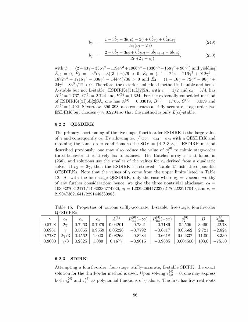
b3 =1− 3b5 − 3b4c
24 − 3γ + 6b5γ + 6b4c4γ
3c3(c3 − 2γ)(249)
b2 =2− 6b5 − 3c3 + 6b5c3 + 6b4c3c4 − 6b4c
24
12γ(2γ − c3), (250)
with φ1 = (2−43γ+336γ2−1194γ3 +1966γ4−1336γ5 +168γ6 +96γ7) and yieldingE10 = 0, E8 = −γ8(γ − 3)(3 + γ)/9 > 0, E6 = (−1 + 24γ − 216γ2 + 912γ3 −1872γ4 + 1716γ5 − 336γ6 − 144γ7)/36 > 0 and E4 = (1 − 16γ + 72γ2 − 96γ3 +24γ4 + 8γ5)/12 > 0. Therefore, the exterior embedded method is I-stable and henceA-stable but not L-stable. ESDIRK4(3)5L[2]SA, with c3 = 1/2 and c4 = 3/4, hasB(5) = 1.767, C(5) = 2.744 and E(5) = 1.324. For the externally embedded methodof ESDIRK4(3I)5L[2]SA, one has A(4) = 0.03019, B(5) = 1.766, C(5) = 3.059 andE(5) = 1.492. Skvortsov [396,398] also constructs a stiffly-accurate, stage-order twoESDIRK but chooses γ ≈ 0.2204 so that the method is only L(α)-stable.
6.2.2 QESDIRK
The primary shortcoming of the five-stage, fourth-order ESDIRK is the large valueof γ and consequently c2. By allowing a22 6= a33 = a44 = a55 with a QESDIRK andretaining the same order conditions as the SOV = {4, 2, 3, 3, 4} ESDIRK method
described previously, one may also reduce the value of q(3)2 to mimic stage-order
three behavior at relatively lax tolerances. The Butcher array is that found in(236), and solutions use the smaller of the values for c3 derived from a quadraticsolve. If c2 = 2γ, then the ESDIRK is retrieved. Table 15 lists three possibleQESDIRKs. Note that the values of γ come from the upper limits listed in Table12. As with the four-stage QESDIRK, only the case where c2 = γ seems worthyof any further consideration; hence, we give the three nontrivial abscissae: c2 =10393270312171/14930336774230, c3 = 12329209447232/21762223217049, and c4 =2190473621641/2291448330983.
Table 15. Properties of various stiffly-accurate, L-stable, five-stage, fourth-orderQESDIRKs.
γ c2 c3 c4 A(5) R(3)int (−∞) R
(4)int (−∞) q
(3)2 D λMmin
0.5728 2γ 0.7263 0.7979 0.04201 −0.7321 −0.7189 0.2506 3.490 −22.780.6961 γ 0.5665 0.9559 0.05226 −0.7792 −0.6417 0.05662 2.721 −2.8240.7787 2γ/3 0.4562 1.023 0.08263 −0.8284 −0.6618 0.02332 11.00 −8.3300.9000 γ/3 0.2825 1.080 0.1677 −0.9015 −0.9685 0.004500 103.6 −75.50
6.2.3 SDIRK
Attempting a fourth-order, four-stage, stiffly-accurate, L-stable SDIRK, the exact
solution for the third-order method is used. Upon solving τ(4)1,2 = 0, one may express
both τ(4)3 and τ
(4)4 as polynomial functions of γ alone. The first has five real roots
86
while the second has four. There are no common roots; hence, there are no fourth-order solutions to this scheme, as proven by Alexander [5].
Relenting on the desire for stiffly-accurate methods, one may derive a two-parameter family (c3 and c4) of L-stable, fourth-order methods with c2 = (3γ(−1 +2γ)2)/(1 − 6γ + 12γ2) and a non-stiffly-accurate analog of (237), implying thatγ = 0.5728160624821348554080014 and c2 ≈ 0.02429. This method is derived by
solving τ(1,2,3,4)1 for b and τ
(3)2 = τ
(4)2,3,4 = 0 for a32, a42, a43 and c2. The minimal
error solution has A(5) = 0.03202 and D = 3.469, but also has a very large negativeeigenvalue of the algebraic stability matrix: −101.3. This situation occurs in theimmediate vicinity of c3 = 11/20 and c4 = 7/9. A more useful solution might beat c3 = 5/7 and c4 = 1/4 with A(5) = 0.05008 and D = 0.7143. Nørsett [308] hasinvestigated this family of methods. In two papers, Jawais et al. [241, 242] studyfour-stage SDIRKs applied to linear ODEs. These methods are fourth-order on lin-ear ODEs but only third-order on nonlinear ODEs. Coroian [119] derives an A- andan L-stable fourth-order SDIRK in four-stages.
6.3 Fifth-Order Methods
6.3.1 ESDIRK
Before attempting to construct a fifth-order ESDIRK in five-stages, one may lookat Table 4 to see that not even A-stable methods are possible. A-stability requiresthat p5 = (1− 20γ+ 120γ2− 240γ3 + 120γ4)/120 = 0. Solving p5 = 0 produces fourroots: γ = 0.09129173346525076086032944, γ = 0.1744841756515234920453601,γ = 0.3888576711028921132337183, and γ = 1.345366419780333633860592; how-ever, none of these values give rise to a positive semidefinite E-polynomial. Hence,none of the methods can be recommended for general stiff equations. However, ifone were to be tested, the γ ≈ 0.3889 root might work best where R(−∞) = 1.038.The form of the method is (233) without the stiffly-accurate assumption. One may
construct this family of methods by solving τ(1,2,3,4,5)1 = q
(2)2,3,4,5 = τ
(4)3 = τ
(5)4,5,8 = 0.
At γ ≈ 0.3889, c4 = 17/27 and c5 = 13/16, A(6) = 0.002758 and the largest internalstability value in the far LHP is−1.755 on stage four. Minimum A(6) for each of theseroots, in ascending magnitude of γ, is A(6) = 0.0004670, 0.0008287, 0.002758, 0.9835.As is commonly observed, smaller values of γ generally correspond to smaller valuesof the leading order error. Kraaijevanger [266] constructs a fifth-order EDIRK witha55 = 0 and A(6) = 0.0002604, in the interest of studying nonlinear contractivity,but the method has Rint(−∞) = {1,−1, 9,−8,∞}.
6.4 Sixth-Order Methods
6.4.1 EDIRK
Al-Rabeh [18] has computed a sixth-order EDIRK in five-stages, four of which areimplicit. It is impossible to make this family of methods A-stable since |R(z)| → ∞as z → −∞ because deg Q(z) = deg P (z) + 1. Al-Rabeh uses assumptions C(2)and D(2) to derive a method with a33 < 0; however, the method can also be
87
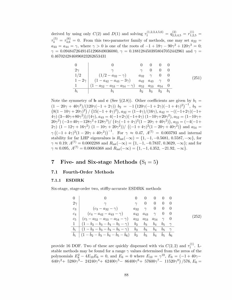
derived by using only C(2) and D(1) and solving τ(1,2,3,4,5,6)1 = q
(2)2,3,4,5 = r
(1)1,2,5 =
τ(5)4 = τ
(6)4,6 = 0. From this two-parameter family of methods, one may set a22 =
a33 = a44 = γ, where γ > 0 is one of the roots of −1 + 18γ − 90γ2 + 120γ3 = 0;γ = 0.09484726491451296849036080, γ = 0.1881284503958047052442961 and γ =0.4670242846896823262653431
0 0 0 0 0 02γ γ γ 0 0 01/2 (1/2− a32 − γ) a32 γ 0 01− 2γ (1− a42 − a43 − 3γ) a42 a43 γ 01 (1− a52 − a53 − a54 − γ) a52 a53 a54 0
bi b1 b2 b3 b2 b1
(251)
Note the symmetry of b and c (See §(2.8)). Other coefficients are given by b1 =
(1 − 20γ + 40γ2)/(120γ(−1 + 2γ)) b2 = −1(120γ(−1 + 2γ)(−1 + 4γ)2
)−1, b3 =(
8(1− 10γ + 20γ)2)/(15(−1 + 4γ)2
), a32 = (1−4γ)/(16γ), a42 = −((−1+2γ)(−1+
4γ) (3−40γ+80γ2))/(4γ), a43 = 4(−1+2γ)(−1+4γ) (1−10γ+20γ2), a52 = (1−10γ+20γ2) (−3+40γ−128γ2+128γ3)/
(4γ(−1 + 4γ)2(1− 20γ + 40γ2)
), a53 = (−4(−1+
2γ) (1 − 12γ + 16γ2) (1 − 10γ + 20γ2))/((−1 + 4γ)2(1− 20γ + 40γ2)
)and a54 =
γ((−1 + 4γ)2(1− 20γ + 40γ2)
)−1. For γ ≈ 0.47, A(7) = 0.003793 and internal
stability for far LHP eigenvalues is Rint(−∞) = {1,−1,−0.5681, 0.5587,−∞}, forγ ≈ 0.19; A(7) = 0.0002288 and Rint(−∞) = {1,−1,−0.7837, 0.3629,−∞}; and forγ ≈ 0.095, A(7) = 0.00004368 and Rint(−∞) = {1,−1, 4.352, −21.92, −∞}.
7 Five- and Six-stage Methods (SI = 5)
7.1 Fourth-Order Methods
7.1.1 ESDIRK
Six-stage, stage-order two, stiffly-accurate ESDIRK methods
0 0 0 0 0 0 02γ γ γ 0 0 0 0c3 (c3 − a32 − γ) a32 γ 0 0 0c4 (c4 − a42 − a43 − γ) a42 a43 γ 0 0c5 (c5 − a52 − a53 − a54 − γ) a52 a53 a54 γ 01 (1− b2 − b3 − b4 − b5 − γ) b2 b3 b4 b5 γ
bi (1− b2 − b3 − b4 − b5 − γ) b2 b3 b4 b5 γ
bi (1− b2 − b3 − b4 − b5 − b6) b2 b3 b4 b5 b6
(252)
provide 16 DOF. Two of these are quickly dispensed with via C(2, 2) and τ(1)1 . L-
stable methods may be found for a range γ values determined from the zeros of thepolynomials E2
8 − 4E10E6 = 0, and E6 = 0 where E10 = γ10, E8 = (−1 + 40γ−640γ2+ 5280γ3− 24240γ4+ 62400γ5− 86400γ6+ 57600γ7− 11520γ8
)/576, E6 =
88
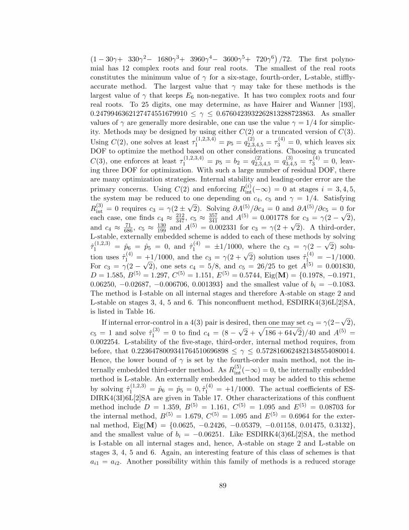
(1− 30γ+ 330γ2− 1680γ3+ 3960γ4− 3600γ5+ 720γ6)/72. The first polyno-
mial has 12 complex roots and four real roots. The smallest of the real rootsconstitutes the minimum value of γ for a six-stage, fourth-order, L-stable, stiffly-accurate method. The largest value that γ may take for these methods is thelargest value of γ that keeps E6 non-negative. It has two complex roots and fourreal roots. To 25 digits, one may determine, as have Hairer and Wanner [193],0.2479946362127474551679910 ≤ γ ≤ 0.6760423932262813288723863. As smallervalues of γ are generally more desirable, one can use the value γ = 1/4 for simplic-ity. Methods may be designed by using either C(2) or a truncated version of C(3).
Using C(2), one solves at least τ(1,2,3,4)1 = p5 = q
(2)2,3,4,5 = τ
(4)3 = 0, which leaves six
DOF to optimize the method based on other considerations. Choosing a truncated
C(3), one enforces at least τ(1,2,3,4)1 = p5 = b2 = q
(2)2,3,4,5 = q
(3)3,4,5 = τ
(4)3 = 0, leav-
ing three DOF for optimization. With such a large number of residual DOF, thereare many optimization strategies. Internal stability and leading-order error are the
primary concerns. Using C(2) and enforcing R(i)int(−∞) = 0 at stages i = 3, 4, 5,
the system may be reduced to one depending on c4, c5 and γ = 1/4. Satisfying
R(3)int = 0 requires c3 = γ(2 ±
√2). Solving ∂A(5)/∂c4 = 0 and ∂A(5)/∂c5 = 0 for
each case, one finds c4 ≈ 212347 , c5 ≈ 357
341 and A(5) = 0.001778 for c3 = γ(2 −√
2),
and c4 ≈ 71686 , c5 ≈ 130
199 and A(5) = 0.002331 for c3 = γ(2 +√
2). A third-order,L-stable, externally embedded scheme is added to each of these methods by solving
τ(1,2,3)1 = p6 = p5 = 0, and τ
(4)1 = ±1/1000, where the c3 = γ(2 −
√2) solu-
tion uses τ(4)1 = +1/1000, and the c3 = γ(2 +
√2) solution uses τ
(4)1 = −1/1000.
For c3 = γ(2 −√
2), one sets c4 = 5/8, and c5 = 26/25 to get A(5) = 0.001830,D = 1.585, B(5) = 1.297, C(5) = 1.151, E(5) = 0.5744, Eig(M) = {0.1978, −0.1971,0.06250, −0.02687, −0.006706, 0.001393} and the smallest value of bi = −0.1083.The method is I-stable on all internal stages and therefore A-stable on stage 2 andL-stable on stages 3, 4, 5 and 6. This nonconfluent method, ESDIRK4(3)6L[2]SA,is listed in Table 16.
If internal error-control in a 4(3) pair is desired, then one may set c3 = γ(2−√
2),
c5 = 1 and solve τ(3)1 = 0 to find c4 = (8 −
√2 +
√186 + 64
√2)/40 and A(5) =
0.002254. L-stability of the five-stage, third-order, internal method requires, frombefore, that 0.2236478009341764510696898 ≤ γ ≤ 0.5728160624821348554080014.Hence, the lower bound of γ is set by the fourth-order main method, not the in-
ternally embedded third-order method. As R(5)int (−∞) = 0, the internally embedded
method is L-stable. An externally embedded method may be added to this scheme
by solving τ(1,2,3)1 = p6 = p5 = 0, τ
(4)1 = +1/1000. The actual coefficients of ES-
DIRK4(3I)6L[2]SA are given in Table 17. Other characterizations of this confluentmethod include D = 1.359, B(5) = 1.161, C(5) = 1.095 and E(5) = 0.08703 forthe internal method, B(5) = 1.679, C(5) = 1.095 and E(5) = 0.6964 for the exter-nal method, Eig(M) = {0.0625, −0.2426, −0.05379, −0.01158, 0.01475, 0.3132},and the smallest value of bi = −0.06251. Like ESDIRK4(3)6L[2]SA, the methodis I-stable on all internal stages and, hence, A-stable on stage 2 and L-stable onstages 3, 4, 5 and 6. Again, an interesting feature of this class of schemes is thatai1 = ai2. Another possibility within this family of methods is a reduced storage
89
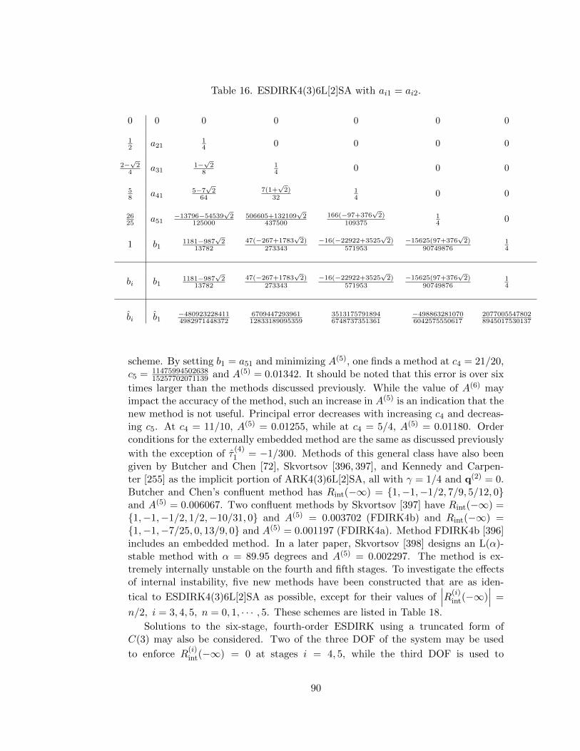
Table 16. ESDIRK4(3)6L[2]SA with ai1 = ai2.
0 0 0 0 0 0 0
12 a21
14 0 0 0 0
2−√2
4 a311−√2
814 0 0 0
58 a41
5−7√2
647(1+
√2)
3214 0 0
2625 a51
−13796−54539√2
125000506605+132109
√2
437500166(−97+376
√2)
10937514 0
1 b11181−987
√2
1378247(−267+1783
√2)
273343−16(−22922+3525
√2)
571953−15625(97+376
√2)
9074987614
bi b11181−987
√2
1378247(−267+1783
√2)
273343−16(−22922+3525
√2)
571953−15625(97+376
√2)
9074987614
bi b1−4809232284114982971448372
670944729396112833189095359
35131757918946748737351361
−4988632810706042575550617
20770055478028945017530137
scheme. By setting b1 = a51 and minimizing A(5), one finds a method at c4 = 21/20,c5 = 11475994502638
15257702071139 and A(5) = 0.01342. It should be noted that this error is over six
times larger than the methods discussed previously. While the value of A(6) mayimpact the accuracy of the method, such an increase in A(5) is an indication that thenew method is not useful. Principal error decreases with increasing c4 and decreas-ing c5. At c4 = 11/10, A(5) = 0.01255, while at c4 = 5/4, A(5) = 0.01180. Orderconditions for the externally embedded method are the same as discussed previously
with the exception of τ(4)1 = −1/300. Methods of this general class have also been
given by Butcher and Chen [72], Skvortsov [396, 397], and Kennedy and Carpen-ter [255] as the implicit portion of ARK4(3)6L[2]SA, all with γ = 1/4 and q(2) = 0.Butcher and Chen’s confluent method has Rint(−∞) = {1,−1,−1/2, 7/9, 5/12, 0}and A(5) = 0.006067. Two confluent methods by Skvortsov [397] have Rint(−∞) ={1,−1,−1/2, 1/2,−10/31, 0} and A(5) = 0.003702 (FDIRK4b) and Rint(−∞) ={1,−1,−7/25, 0, 13/9, 0} and A(5) = 0.001197 (FDIRK4a). Method FDIRK4b [396]includes an embedded method. In a later paper, Skvortsov [398] designs an L(α)-stable method with α = 89.95 degrees and A(5) = 0.002297. The method is ex-tremely internally unstable on the fourth and fifth stages. To investigate the effectsof internal instability, five new methods have been constructed that are as iden-
tical to ESDIRK4(3)6L[2]SA as possible, except for their values of∣∣∣R(i)
int(−∞)∣∣∣ =
n/2, i = 3, 4, 5, n = 0, 1, · · · , 5. These schemes are listed in Table 18.
Solutions to the six-stage, fourth-order ESDIRK using a truncated form ofC(3) may also be considered. Two of the three DOF of the system may be used
to enforce R(i)int(−∞) = 0 at stages i = 4, 5, while the third DOF is used to
90
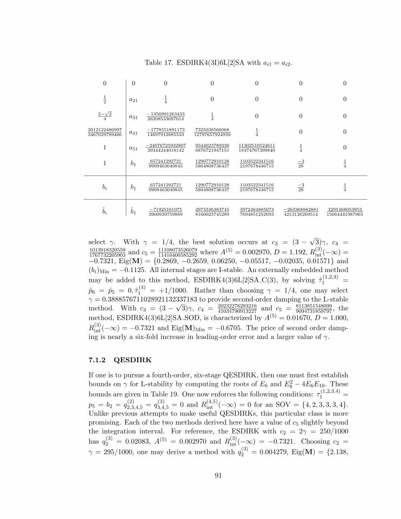
Table 17. ESDIRK4(3I)6L[2]SA with ai1 = ai2.
0 0 0 0 0 0 0
12 a21
14 0 0 0 0
2−√2
4 a31−135699126343326208533697614
14 0 0 0
20121224869973467029789466 a41
−177855189117314697912885533
732503856606812797657924939
14 0 0
1 a51−2407672593280739344244018142
93440237893306876721947151
1130251052461118374767399840
14 0
1 b16572412927219909463049845
12907729101285804808736437
11035223415162197678446715
−328
14
bi b16572412927219909463049845
12907729101285804808736437
11035223415162197678446715
−328
14
bi b1−719251610753900939759889
29733463837458160025745289
39724648850737694851252693
−2633688828814213126269514
329546805395315064441987965
select γ. With γ = 1/4, the best solution occurs at c3 = (3 −√
3)γ, c4 =10139183205591767732205903 and c5 = 11108073526079
11410400585292 where A(5) = 0.002970, D = 1.192, R(3)int (−∞) =
−0.7321, Eig(M) = {0.2869, −0.2659, 0.06250, −0.05517, −0.02035, 0.01571} and(bi)Min = −0.1125. All internal stages are I-stable. An externally embedded method
may be added to this method, ESDIRK4(3)6L[2]SA C(3), by solving τ(1,2,3)1 =
p6 = p5 = 0, τ(4)1 = +1/1000. Rather than choosing γ = 1/4, one may select
γ = 0.3888576711028921132337183 to provide second-order damping to the L-stablemethod. With c3 = (3 −
√3)γ, c4 = 20232276293216
41034790913227 and c5 = 81138515480999094731859797 , the
method, ESDIRK4(3)6L[2]SA SOD, is characterized by A(5) = 0.01670, D = 1.000,
R(3)int (−∞) = −0.7321 and Eig(M)Min = −0.6705. The price of second order damp-
ing is nearly a six-fold increase in leading-order error and a larger value of γ.
7.1.2 QESDIRK
If one is to pursue a fourth-order, six-stage QESDIRK, then one must first establishbounds on γ for L-stability by computing the roots of E6 and E2
8 − 4E6E10. These
bounds are given in Table 19. One now enforces the following conditions: τ(1,2,3,4)1 =
p5 = b2 = q(2)2,3,4,5 = q
(3)3,4,5 = 0 and R
(4,5)int (−∞) = 0 for an SOV = {4, 2, 3, 3, 3, 4}.
Unlike previous attempts to make useful QESDIRKs, this particular class is morepromising. Each of the two methods derived here have a value of c5 slightly beyondthe integration interval. For reference, the ESDIRK with c2 = 2γ = 250/1000
has q(3)2 = 0.02083, A(5) = 0.002970 and R
(3)int (−∞) = −0.7321. Choosing c2 =
γ = 295/1000, one may derive a method with q(3)2 = 0.004279, Eig(M) = {2.138,
91
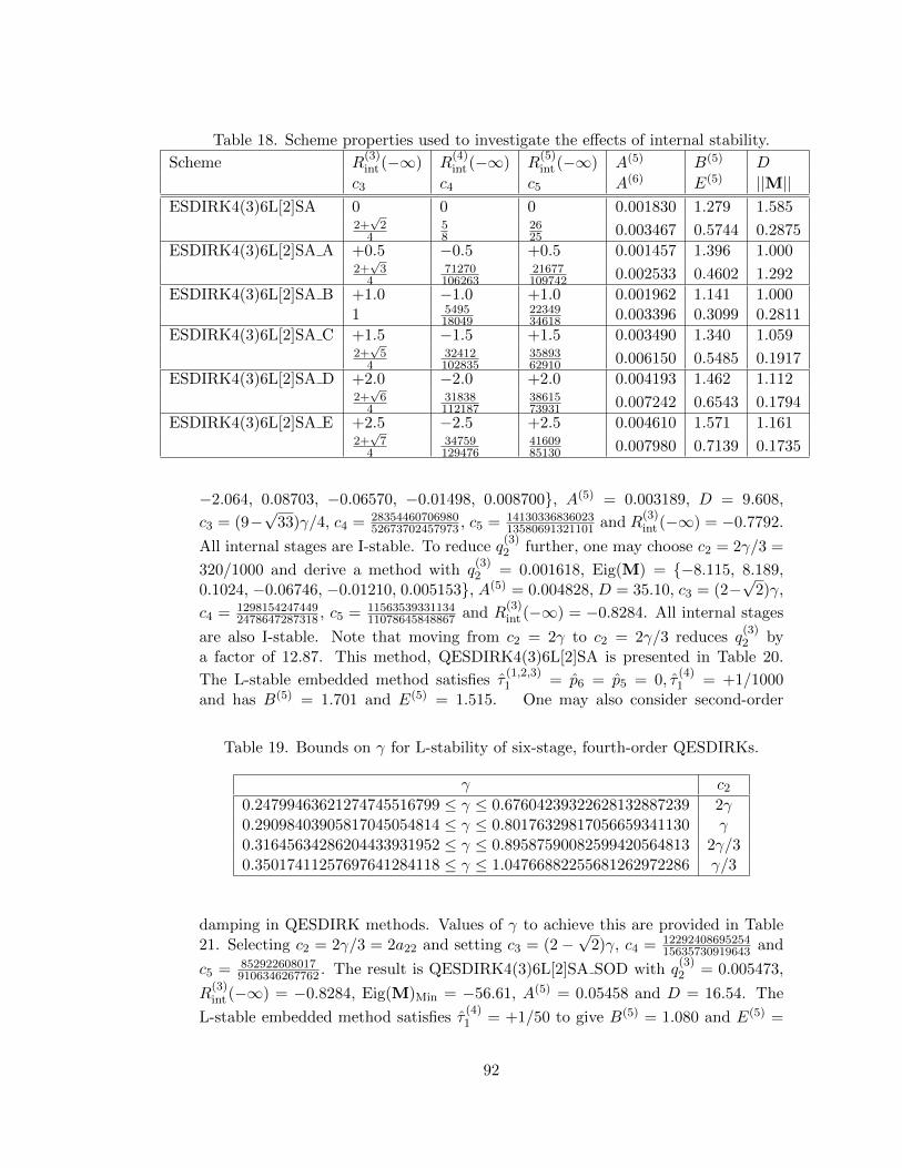
Table 18. Scheme properties used to investigate the effects of internal stability.
Scheme R(3)int (−∞) R
(4)int (−∞) R
(5)int (−∞) A(5) B(5) D
c3 c4 c5 A(6) E(5) ||M||ESDIRK4(3)6L[2]SA 0 0 0 0.001830 1.279 1.585
2+√
24
58
2625 0.003467 0.5744 0.2875
ESDIRK4(3)6L[2]SA A +0.5 −0.5 +0.5 0.001457 1.396 1.0002+√
34
71270106263
21677109742 0.002533 0.4602 1.292
ESDIRK4(3)6L[2]SA B +1.0 −1.0 +1.0 0.001962 1.141 1.0001 5495
180492234934618 0.003396 0.3099 0.2811
ESDIRK4(3)6L[2]SA C +1.5 −1.5 +1.5 0.003490 1.340 1.0592+√
54
32412102835
3589362910 0.006150 0.5485 0.1917
ESDIRK4(3)6L[2]SA D +2.0 −2.0 +2.0 0.004193 1.462 1.1122+√
64
31838112187
3861573931 0.007242 0.6543 0.1794
ESDIRK4(3)6L[2]SA E +2.5 −2.5 +2.5 0.004610 1.571 1.1612+√
74
34759129476
4160985130 0.007980 0.7139 0.1735
−2.064, 0.08703, −0.06570, −0.01498, 0.008700}, A(5) = 0.003189, D = 9.608,
c3 = (9−√
33)γ/4, c4 = 2835446070698052673702457973 , c5 = 14130336836023
13580691321101 and R(3)int (−∞) = −0.7792.
All internal stages are I-stable. To reduce q(3)2 further, one may choose c2 = 2γ/3 =
320/1000 and derive a method with q(3)2 = 0.001618, Eig(M) = {−8.115, 8.189,
0.1024, −0.06746, −0.01210, 0.005153}, A(5) = 0.004828, D = 35.10, c3 = (2−√
2)γ,
c4 = 12981542474492478647287318 , c5 = 11563539331134
11078645848867 and R(3)int (−∞) = −0.8284. All internal stages
are also I-stable. Note that moving from c2 = 2γ to c2 = 2γ/3 reduces q(3)2 by
a factor of 12.87. This method, QESDIRK4(3)6L[2]SA is presented in Table 20.
The L-stable embedded method satisfies τ(1,2,3)1 = p6 = p5 = 0, τ
(4)1 = +1/1000
and has B(5) = 1.701 and E(5) = 1.515. One may also consider second-order
Table 19. Bounds on γ for L-stability of six-stage, fourth-order QESDIRKs.
γ c2
0.24799463621274745516799 ≤ γ ≤ 0.67604239322628132887239 2γ0.29098403905817045054814 ≤ γ ≤ 0.80176329817056659341130 γ0.31645634286204433931952 ≤ γ ≤ 0.89587590082599420564813 2γ/30.35017411257697641284118 ≤ γ ≤ 1.04766882255681262972286 γ/3
damping in QESDIRK methods. Values of γ to achieve this are provided in Table21. Selecting c2 = 2γ/3 = 2a22 and setting c3 = (2−
√2)γ, c4 = 12292408695254
15635730919643 and
c5 = 8529226080179106346267762 . The result is QESDIRK4(3)6L[2]SA SOD with q
(3)2 = 0.005473,
R(3)int (−∞) = −0.8284, Eig(M)Min = −56.61, A(5) = 0.05458 and D = 16.54. The
L-stable embedded method satisfies τ(4)1 = +1/50 to give B(5) = 1.080 and E(5) =
92
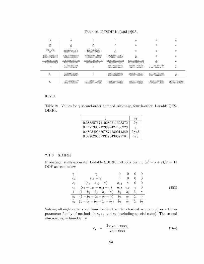
Table 20. QESDIRK4(3)6L[2]SA.
0 0 0 0 0 0 0
1675
875
875
0 0 0 0
8(2−√
2)25
6054978619789136257189845
−212784879855110702252975294
825
0 0 0
12981542474492478647287318
−30051066869556150333508049
−6866266819379911091168490809
8078689811082211737001380747
825
0 0
1156353933113411078645848867
−261628055588468363194173203
−2919872959644879066074244437
38468289227867010959450712301
1355554845110214148104892819
825
0
1 5400882386974693226184761
0 10947624909947880993776667
40165647630037185357966874
−4118202588273096789411938
825
bi5400882386974693226184761
0 10947624909947880993776667
40165647630037185357966874
−4118202588273096789411938
825
bi−3744843266778442488809460
−4112509115993825963879779069
2402508827049412927594097169
51939174613018985383982321
−184312200183016078617943063
24395722129727960792257433
0.7701.
Table 21. Values for γ second-order damped, six-stage, fourth-order, L-stable QES-DIRKs.
γ c2
0.38885767110289211323372 2γ0.44773852423399424486223 γ0.48034935707874730014389 2γ/30.52202633733470430577704 γ/3
7.1.3 SDIRK
Five-stage, stiffly-accurate, L-stable SDIRK methods permit (s2 − s + 2)/2 = 11DOF as seen below
γ γ 0 0 0 0c2 (c2 − γ) γ 0 0 0c3 (c3 − a32 − γ) a32 γ 0 0c4 (c4 − a42 − a43 − γ) a42 a43 γ 01 (1− b2 − b3 − b4 − γ) b2 b3 b4 γ
bi (1− b2 − b3 − b4 − γ) b2 b3 b4 γ
bi (1− b2 − b3 − b4 − b5) b2 b3 b4 b5
(253)
Solving all eight order conditions for fourth-order classical accuracy gives a three-parameter family of methods in γ, c3 and c4 (excluding special cases). The secondabscissa, c2, is found to be
c2 =3γ(ϕ1 + c4ϕ1)
ϕ3 + c4ϕ4(254)
93
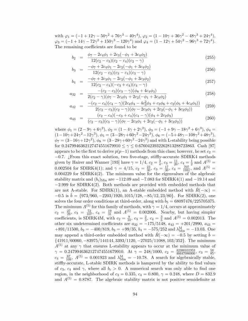
with ϕ1 = (−1 + 12γ − 50γ2 + 76γ3 − 40γ4), ϕ2 = (1− 10γ + 36γ2 − 48γ3 + 24γ4),ϕ3 = (−1 + 14γ − 72γ2 + 150γ3 − 120γ4) and ϕ4 = (1− 12γ + 54γ2 − 96γ3 + 72γ4).The remaining coefficients are found to be
b2 =φ7 − 2c4φ1 + 2c3(−φ1 + 3c4φ2)
12(c2 − c3)(c2 − c4)(c2 − γ)(255)
b3 =−φ7 + 2c4φ1 − 2c2(−φ1 + 3c4φ2)
12(c2 − c3)(c3 − c4)(c3 − γ)(256)
b4 =−φ7 + 2c3φ1 − 2c2(−φ1 + 3c3φ2)
12(c2 − c4)(−c3 + c4)(c4 − γ)(257)
a32 =−(c2 − c3)(c3 − γ)(φ8 + 4c4φ3)
2(c2 − γ)(φ7 − 2c4φ1 + 2c2(−φ1 + 3c4φ2)(258)
a42 =−(c2 − c4)(c4 − γ)(2c4φ4 − 4c2
3φ3 + c3φ6 + c2(φ5 + 4c4φ3))
2(c2 − c3)(c2 − γ)(φ7 − 2c3φ1 + 2c2(−φ1 + 3c3φ2))(259)
a43 =(c2 − c4)(−c3 + c4)(c4 − γ)(φ4 + 2c2φ3)
(c2 − c3)(c3 − γ)(φ7 − 2c3φ1 + 2c2(−φ1 + 3c3φ2))(260)
where φ1 = (2− 9γ + 6γ2), φ2 = (1− 4γ + 2γ2), φ3 = (−1 + 9γ − 18γ2 + 6γ3), φ4 =(1−10γ+24γ2−12γ3), φ5 = (3−28γ+60γ2−24γ3), φ6 = (−5+48γ−108γ2+48γ3),φ7 = (3−16γ+12γ2), φ8 = (3−28γ+60γ2−24γ3) and with L-stability being possiblefor 0.2479946362127474551679910 ≤ γ ≤ 0.6760423932262813288723863. Cash [97]appears to be the first to derive p(p−1) methods from this class; however, he set c2 =−0.7. ¿From this exact solution, two five-stage, stiffly-accurate SDIRK4 methodsgiven by Hairer and Wanner [193] have γ = 1/4, c2 = 3
4 , c3 = 1120 , c4 = 1
2 and A(5) =
0.002504 for SDIRK4(1); and γ = 4/15, c2 = 2330 , c3 = 17
30 , c4 = 7071931 , and A(5) =
0.004229 for SDIRK4(2). The minimum value for the eigenvalues of the algebraicstability matrix and (bi)Min are −112.09 and −7.083 for SDIRK4(1) and −19.14 and−2.999 for SDIRK4(2). Both methods are provided with embedded methods thatare not A-stable. For SDIRK(1), an A-stable embedded method with R(−∞) =−0.5 is b = {973/960,−2203/1920, 1015/128,−85/12, 23/80}. For SDIRK(2), onesolves the four order conditions at third-order, along with b5 = 68097476/225705375.The minimum A(5) for this family of methods, with γ = 1/4, occurs at approximatelyc2 = 27
29 , c3 = 72107 , c4 = 19
31 and A(5) = 0.002006. Nearby, but having simpler
coefficients, is SDIRK4M, with c2 = 910 , c3 = 2
3 , c4 = 35 and A(5) = 0.002013. The
other six undetermined coefficients are a32 = −175/5148, a42 = +201/2990, a43 =+891/11500, b2 = −400/819, b3 = +99/35, b4 = −575/252 and λM
Min = −13.03. One
may append a third-order embedded method with R(−∞) = −0.5 by setting b ={41911/60060,−83975/144144, 3393/1120,−27025/11088, 103/352}. The minimumA(5) at any γ that ensures L-stability appears to occur at the minimum value ofγ = 0.2479946362127474551679910. At γ = 248/1000, c2 = 42380101953
46647086000 , c3 = 5885 ,
c4 = 67109 , A(5) = 0.001923 and λM
Min = −10.78. A search for algebraically stable,stiffly-accurate, L-stable SDIRK methods is hampered by the ability to find valuesof c3, c4 and γ, where all bi > 0. A numerical search was only able to find oneregion, in the neighborhood of c3 = 0.335, c4 = 0.800, γ = 0.248, where D = 832.9and A(5) = 0.8787. The algebraic stability matrix is not positive semidefinite at
94
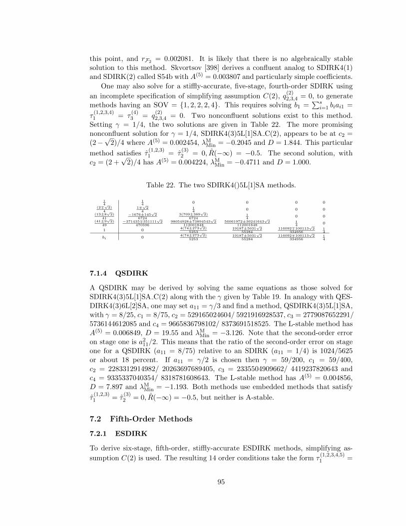
this point, and rF2 = 0.002081. It is likely that there is no algebraically stablesolution to this method. Skvortsov [398] derives a confluent analog to SDIRK4(1)and SDIRK(2) called S54b with A(5) = 0.003807 and particularly simple coefficients.
One may also solve for a stiffly-accurate, five-stage, fourth-order SDIRK using
an incomplete specification of simplifying assumption C(2), q(2)2,3,4 = 0, to generate
methods having an SOV = {1, 2, 2, 2, 4}. This requires solving b1 =∑s
i=1 biai1 =
τ(1,2,3,4)1 = τ
(4)3 = q
(2)2,3,4 = 0. Two nonconfluent solutions exist to this method.
Setting γ = 1/4, the two solutions are given in Table 22. The more promisingnonconfluent solution for γ = 1/4, SDIRK4(3)5L[1]SA C(2), appears to be at c2 =(2−
√2)/4 where A(5) = 0.002454, λM
Min = −0.2045 and D = 1.844. This particular
method satisfies τ(1,2,3)1 = τ
(3)2 = 0, R(−∞) = −0.5. The second solution, with
c2 = (2 +√
2)/4 has A(5) = 0.004224, λMMin = −0.4711 and D = 1.000.
Table 22. The two SDIRK4()5L[1]SA methods.
14
14
0 0 0 0(2∓√
2)4
1∓√
24
14
0 0 0(13±8
√2)
41−1676±145
√2
67243(709±389
√2)
672414
0 0(41±9
√2)
49−371435∓351111
√2
47059698054928±73894543
√2
11200184856061972±30241643
√2
11200184814
0
1 04(74±273
√2)
525319187±5031
√2
55284116092∓100113
√2
33495614
bi 04(74±273
√2)
525319187±5031
√2
55284116092∓100113
√2
33495614
7.1.4 QSDIRK
A QSDIRK may be derived by solving the same equations as those solved forSDIRK4(3)5L[1]SA C(2) along with the γ given by Table 19. In analogy with QES-DIRK4(3)6L[2]SA, one may set a11 = γ/3 and find a method, QSDIRK4(3)5L[1]SA,with γ = 8/25, c1 = 8/75, c2 = 529165024604/ 5921916928537, c3 = 2779087652291/5736144612085 and c4 = 9665836798102/ 8373691518525. The L-stable method hasA(5) = 0.006849, D = 19.55 and λM
Min = −3.126. Note that the second-order erroron stage one is a2
11/2. This means that the ratio of the second-order error on stageone for a QSDIRK (a11 = 8/75) relative to an SDIRK (a11 = 1/4) is 1024/5625or about 18 percent. If a11 = γ/2 is chosen then γ = 59/200, c1 = 59/400,c2 = 2283312914982/ 20263697689405, c3 = 2335504909662/ 4419237820643 andc4 = 9335337040354/ 8318781608643. The L-stable method has A(5) = 0.004856,D = 7.897 and λM
Min = −1.193. Both methods use embedded methods that satisfy
τ(1,2,3)1 = τ
(3)2 = 0, R(−∞) = −0.5, but neither is A-stable.
7.2 Fifth-Order Methods
7.2.1 ESDIRK
To derive six-stage, fifth-order, stiffly-accurate ESDIRK methods, simplifying as-
sumption C(2) is used. The resulting 14 order conditions take the form τ(1,2,3,4,5)1 =
95
p5 = τ(4)3 = τ
(5)4,5,8 = q
(2)2,3,4,5 = 0, leaving a two-parameter family of methods in terms
of c4 and c5 with
c3 =4γ(−1 + 16γ − 92γ2 + 212γ3 − 180γ4 + c5ω1)
−1 + 18γ − 120γ2 + 336γ3 − 360γ4 + c5ω2
(261)
and ω1 = 1 − 14γ + 72γ2 − 150γ3 + 120γ4, ω2 = 1 − 16γ + 96γ2 − 240γ3 + 240γ4,E10 = (1 − 10γ + 20γ2)(1 − 15γ + 30γ2)(−1 + 25γ − 200γ2 + 600γ3 − 600γ4 +240γ5)/14400, E8 = (3−120γ+1880γ2−14880γ3+63600γ4−144960γ5+158400γ6−57600γ7)/2880, E6 = (−1 + 30γ − 300γ2 + 1200γ3 − 1800γ4 + 720γ5)/360 and
R(3)int (−∞) =
(c2
3 − 4c3γ + 2γ2)/(2γ2). Expressions for the Runge-Kutta coeffi-
cients, R(4)int (−∞), R
(5)int (−∞) and A(6), are too cumbersome to include. For L-
stability of the overall scheme, γ must be a root of the polynomial 1−25γ+200γ2−600γ3 + 600γ4 − 120γ5 = 0. Only one of the five roots that ensures R(−∞) = 0also provides I-stability: γ ≈ 0.2780538411364523249315862. Upon inspection of
|R(3)int (−∞)|, |R(4)
int (−∞)|, and |R(5)int (−∞)|, it may be determined that if both c4 and
c5 remain positive, that internal stability for very stiff scaled eigenvalues is only pos-sible for specific regions within 0 ≤ c4 ≤ 0.20782427518534172606939559 and 0 ≤c5 ≤ 0.23111961220951036305109788. Enforcing R
(4)int (−∞) = 0 and R
(5)int (−∞) = 0
forces c4 = c5 = 0.07838319999965920091902891 and R(3)int (−∞) = 0.4876; however,
because b4 and b5 are each proportional to (c4 − c5)−1, they become infinite. Sep-
arating the two abscissae a bit, at c4 = 1/10 and c5 = 3/50, R(3)int (−∞) = 0.4438,
R(4)int (−∞) = −0.2198, R
(5)int (−∞) = 0.4549 and A(6) = 0.004615. Stages 2, 3 and
6 are I-stable but stages 4 and 5 are not. It appears to be impossible to make allstages I-stable with positive abscissae. A third-order, L-stable, externally embedded
method may be done as τ(1,2,3)1 = p6 = p5 = 0, and τ
(4)1 = −1/500. The result-
ing 5(3) method, ESDIRK5(3)6L[2]SA, appears in Table 23. Other schemes arepossible. One may attempt third-order internal error-control by setting c5 = 1 andimplying c3 = 4γ(−1+2γ)(−1+3γ)(−1+5γ)
−1+12γ−48γ2+60γ3≈ −0.3778. As this value is quite undesirable,
internal error-control for this method cannot be recommended. Next, one can min-
imize sixth-order error by solving ∂A(6)
∂c4= ∂A(6)
∂c5= 0 to get c4 ≈ 5935807227
8309450038 ≈ 0.7143,
c5 ≈ 1870598988315763987604 ≈ 1.187, R
(3)int (−∞) = −0.08432, R
(4)int (−∞) = −2.930, R
(5)int (−∞) =
−3.615 and A(6) = 0.002005. Again, this scheme cannot be recommended because ofinternal instability. Including a fourth-order, A-stable externally embedded methodto the internally stable main method given previously is not possible without using
the main method to satisfy τ(4)3 = 0. Reduced storage and conditionally contractive
methods are not pursued because of the small ranges of c4 and c5 that give rise tointernally stable methods. Skvortsov [396, 398] construct fifth-order methods butselects γ ≈ 0.1411. In an earlier paper, Skvortsov [396] designs a method that hasA(6) = 0.007660 and c4 = 4/3. A later paper [398] constructs an L(α)-stable method,ES65, with α = 72.3 degrees. Shintani [384] achieves fifth-order but without usingthe stiffly-accurate assumption.
For completeness, one may also derive six-stage, fifth-order, stiffly-accurate ES-
96
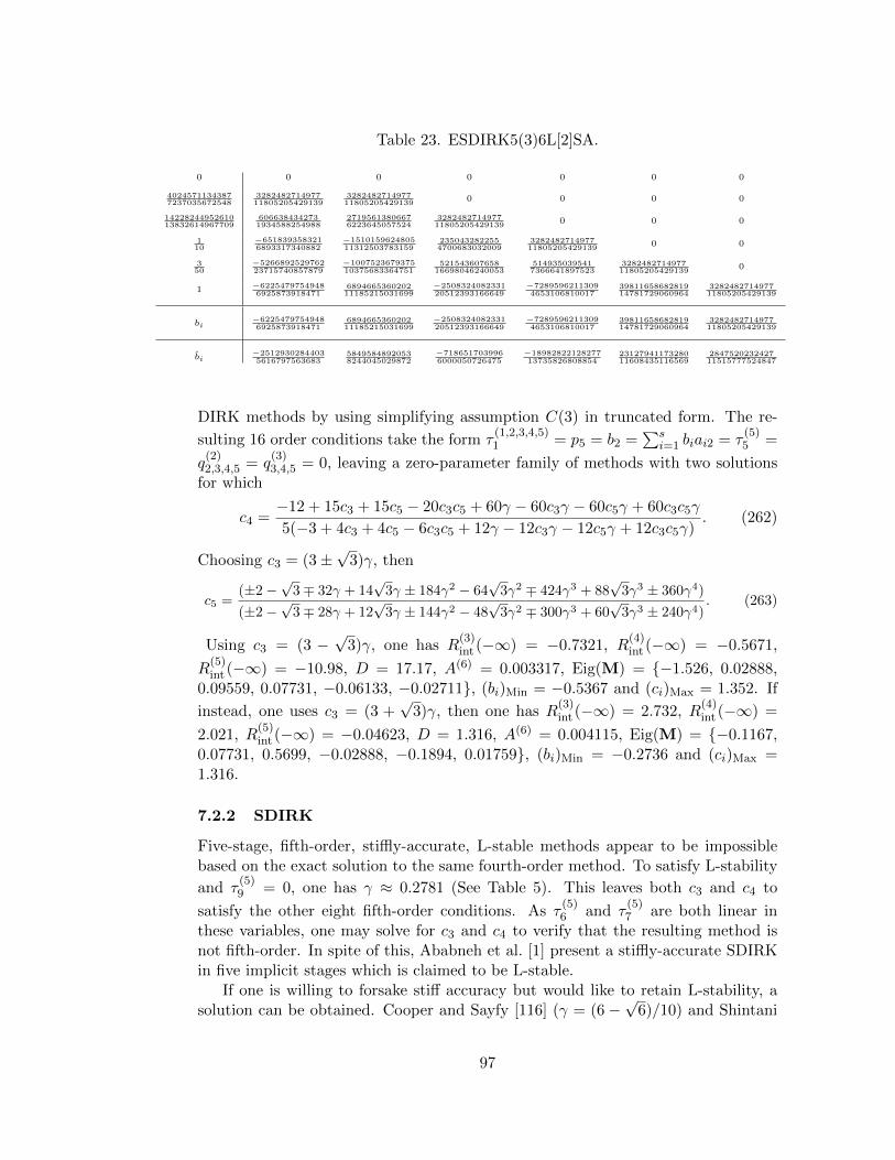
Table 23. ESDIRK5(3)6L[2]SA.
0 0 0 0 0 0 0
40245711343877237035672548
328248271497711805205429139
328248271497711805205429139
0 0 0 0
1422824495261013832614967709
6066384342731934588254988
27195613806676223645057524
328248271497711805205429139
0 0 0
110
−6518393583216893317340882
−151015962480511312503783159
2350432822554700683032009
328248271497711805205429139
0 0
350
−526689252976223715740857879
−100752367937510375683364751
52154360765816698046240053
5149350395417366641897523
328248271497711805205429139
0
1 −62254797549486925873918471
689466536020211185215031699
−250832408233120512393166649
−72895962113094653106810017
3981165868281914781729060964
328248271497711805205429139
bi−62254797549486925873918471
689466536020211185215031699
−250832408233120512393166649
−72895962113094653106810017
3981165868281914781729060964
328248271497711805205429139
bi−25129302844035616797563683
58495848920538244045029872
−7186517039966000050726475
−1898282212827713735826808854
2312794117328011608435116569
284752023242711515777524847
DIRK methods by using simplifying assumption C(3) in truncated form. The re-
sulting 16 order conditions take the form τ(1,2,3,4,5)1 = p5 = b2 =
∑si=1 biai2 = τ
(5)5 =
q(2)2,3,4,5 = q
(3)3,4,5 = 0, leaving a zero-parameter family of methods with two solutions
for which
c4 =−12 + 15c3 + 15c5 − 20c3c5 + 60γ − 60c3γ − 60c5γ + 60c3c5γ
5(−3 + 4c3 + 4c5 − 6c3c5 + 12γ − 12c3γ − 12c5γ + 12c3c5γ). (262)
Choosing c3 = (3±√
3)γ, then
c5 =(±2−
√3∓ 32γ + 14
√3γ ± 184γ2 − 64
√3γ2 ∓ 424γ3 + 88
√3γ3 ± 360γ4)
(±2−√
3∓ 28γ + 12√
3γ ± 144γ2 − 48√
3γ2 ∓ 300γ3 + 60√
3γ3 ± 240γ4). (263)
Using c3 = (3 −√
3)γ, one has R(3)int (−∞) = −0.7321, R
(4)int (−∞) = −0.5671,
R(5)int (−∞) = −10.98, D = 17.17, A(6) = 0.003317, Eig(M) = {−1.526, 0.02888,
0.09559, 0.07731, −0.06133, −0.02711}, (bi)Min = −0.5367 and (ci)Max = 1.352. If
instead, one uses c3 = (3 +√
3)γ, then one has R(3)int (−∞) = 2.732, R
(4)int (−∞) =
2.021, R(5)int (−∞) = −0.04623, D = 1.316, A(6) = 0.004115, Eig(M) = {−0.1167,
0.07731, 0.5699, −0.02888, −0.1894, 0.01759}, (bi)Min = −0.2736 and (ci)Max =1.316.
7.2.2 SDIRK
Five-stage, fifth-order, stiffly-accurate, L-stable methods appear to be impossiblebased on the exact solution to the same fourth-order method. To satisfy L-stability
and τ(5)9 = 0, one has γ ≈ 0.2781 (See Table 5). This leaves both c3 and c4 to
satisfy the other eight fifth-order conditions. As τ(5)6 and τ
(5)7 are both linear in
these variables, one may solve for c3 and c4 to verify that the resulting method isnot fifth-order. In spite of this, Ababneh et al. [1] present a stiffly-accurate SDIRKin five implicit stages which is claimed to be L-stable.
If one is willing to forsake stiff accuracy but would like to retain L-stability, asolution can be obtained. Cooper and Sayfy [116] (γ = (6 −
√6)/10) and Shintani
97
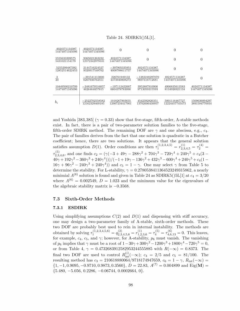
Table 24. SDIRK5()5L[1].
402457113438714474071345096
402457113438714474071345096 0 0 0 0
55556333995755431021154178
936502126323212572342979331
402457113438714474071345096 0 0 0
525529948739212852514622453
21447162245279320917548702
−3979053359514008788611757
402457113438714474071345096 0 0
320
−2915414130006267936762551
2267619491324473940808273
−12822482970709697416712681
402457113438714474071345096 0
1044950021070914474071345096
−24816795160574626464057815
−1971124226876604378783090
39528879109069713059315593
49068356135838134926921134
402457113438714474071345096
bi−252270255858212162329469185
101826790365512907234417901
454239282635113702606430957
500111646772712224457745473
15096360942973891594770934
and Yoshida [383,385] (γ = 0.33) show that five-stage, fifth-order, A-stable methodsexist. In fact, there is a pair of two-parameter solution families to the five-stage,fifth-order SDIRK method. The remaining DOF are γ and one abscissa, e.g., c4.The pair of families derives from the fact that one solution is quadratic in a Butchercoefficient; hence, there are two solutions. It appears that the general solution
satisfies assumption D(1). Order conditions are then τ(1,2,3,4,5)1 = r
(1)2,3,4,5 = τ
(4)2 =
τ(5)2,3,4,6, and one finds c2 = (γ(−3 + 49γ − 288γ2 + 704γ3 − 720γ4 + 240γ5 + c4(3 −
40γ+ 192γ2−360γ3 + 240γ4)))/(−1 + 19γ−136γ2 + 432γ3−600γ4 + 240γ5 + c4(1−16γ + 96γ2 − 240γ3 + 240γ4)) and c5 = 1 − γ. One may select γ from Table 5 todetermine the stability. For L-stability, γ = 0.2780538411364523249315862, a nearlyminimial A(6) solution is found and given in Table 24 as SDIRK5()5L[1] at c4 = 3/20where A(6) = 0.002549, D = 1.023 and the minimum value for the eigenvalues ofthe algebraic stability matrix is −0.3568.
7.3 Sixth-Order Methods
7.3.1 ESDIRK
Using simplifying assumptions C(2) and D(1) and dispensing with stiff accuracy,one may design a two-parameter family of A-stable, sixth-order methods. Thesetwo DOF are probably best used to rein in internal instability. The methods are
obtained by solving τ(1,2,3,4,5,6)1 = q
(2)2,3,4,5,6 = r
(1)1,2,3,6 = τ
(5)4 = τ
(6)4,6,13 = 0. This leaves,
for example, c4, c5, and γ; however, for A-stability, p6 must vanish. The vanishingof p6 implies that γ must be a root of 1−30γ+300γ2−1200γ3 +1800γ4−720γ5 = 0,or from Table 4, γ = 0.4732683912582953244555885 with R(−∞) = 0.8373. The
final two DOF are used to control R(i)int(−∞); c4 = 2/5 and c5 = 81/100. The
resulting method has c3 = 210618880064/9718174947659, c6 = 1 − γ, Rint(−∞) ={1,−1, 0.9095,−0.9710, 0.9873, 0.3560}, D = 22.83, A(7) = 0.004899 and Eig(M) ={5.480, −5.056, 0.2286, −0.06744, 0.0002664, 0}.
98
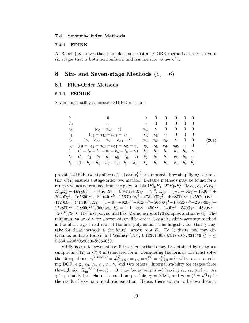
7.4 Seventh-Order Methods
7.4.1 EDIRK
Al-Rabeh [18] proves that there does not exist an EDIRK method of order seven insix-stages that is both nonconfluent and has nonzero values of bi.
8 Six- and Seven-stage Methods (SI = 6)
8.1 Fifth-Order Methods
8.1.1 ESDIRK
Seven-stage, stiffly-accurate ESDIRK methods
0 0 0 0 0 0 0 02γ γ γ 0 0 0 0 0c3 (c3 − a32 − γ) a32 γ 0 0 0 0c4 (c4 − a42 − a43 − γ) a42 a43 γ 0 0 0c5 (c5 − a52 − a53 − a54 − γ) a52 a53 a54 γ 0 0c6 (c6 − a62 − a63 − a64 − a65 − γ) a62 a63 a64 a65 γ 01 (1− b2 − b3 − b4 − b5 − b6 − γ) b2 b3 b4 b5 b6 γ
bi (1− b2 − b3 − b4 − b5 − b6 − γ) b2 b3 b4 b5 b6 γ
bi (1− b2 − b3 − b4 − b5 − b6 − b7) b2 b3 b4 b5 b6 b7
(264)
provide 22 DOF, twenty after C(2, 2) and τ(1)1 are imposed. Row simplifying assump-
tion C(2) ensures a stage-order two method. L-stable methods may be found for arange γ values determined from the polynomials 4E3
10E6+27E212E
26−18E12E10E8E6−
E210E
28 + 4E12E
38 = 0 and E6 = 0 where E12 = γ12, E10 = (−1 + 60γ − 1500γ2 +
20400γ3−165600γ4 +829440γ5−2563200γ6 +4752000γ7−4968000γ8 +2592000γ9−432000γ10)/14400, E8 = (1−48γ+920γ2−9120γ3+50400γ4−155520γ5+250560γ6−172800γ7 +28800γ8)/960 and E6 = (−1+36γ−450γ2 +2400γ3−5400γ4 +4320γ5−720γ6)/360. The first polynomial has 32 unique roots (26 complex and six real). Theminimum value of γ for a seven-stage, fifth-order, L-stable, stiffly-accurate methodis the fifth largest real root of the first polynomial. The largest value that γ maytake for these methods is the fourth largest root E6. To 25 digits, one may de-termine, as have Hairer and Wanner [193], 0.1839146536751751632321436 ≤ γ ≤0.3341423670680504359540301.
Stiffly accurate, seven-stage, fifth-order methods may be obtained by using as-sumptions C(2) or C(3) in truncated form. Considering the former, one must solve
the 15 equations, τ(1,2,3,4,5)1 = q
(2)2,3,4,5,6 = p6 = τ
(4)3 = τ
(5)4,5,8 = 0, with seven remain-
ing DOF, e.g., c3, c4, c5, c6, γ, and two others. Internal stability for stages three
through six, R(3,4,5,6)int (−∞) = 0, may be accomplished leaving c4, c6, and γ. As
γ is probably best chosen as small as possible, γ = 0.184, and c3 = (2 ±√
2)γ isthe result of solving a quadratic equation. Hence, there appear to be two distinct
99
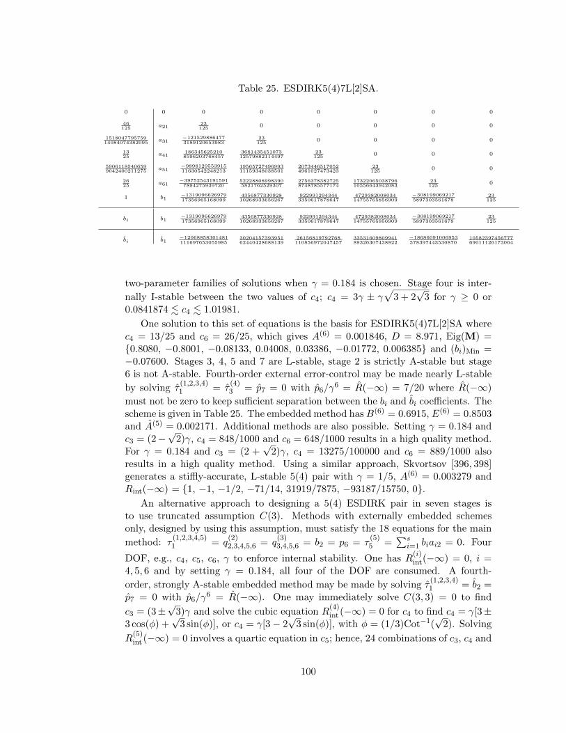
Table 25. ESDIRK5(4)7L[2]SA.
0 0 0 0 0 0 0 0
46125
a2123125
0 0 0 0 0
151804779575914084074382095
a31−1215298864773189120653983
23125
0 0 0 0
1325
a411863456252108596203768457
368143545107312579882114497
23125
0 0 0
59061185406599042400211275
a51−989812955391511630542248213
1956572749699311159348038501
20734465170524961027473423
23125
0 0
2625
a61−397525431915917894275939720
522288089983905821762529307
27563783827258748785577174
1732206503879610556643942083
23125
0
1 b1−131909662697917356965168099
435687733092810268933656267
9229912943443350617878647
472938200803414755765856909
−3081990692175897303561678
23125
bi b1−131909662697917356965168099
435687733092810268933656267
9229912943443350617878647
472938200803414755765856909
−3081990692175897303561678
23125
bi b1−12068858301481111697653055985
3020415739395162440428688139
26156819792768110856972047457
3353160980994189326307438822
−18686091006953578397443530870
1058239745677769011126173064
two-parameter families of solutions when γ = 0.184 is chosen. Stage four is inter-
nally I-stable between the two values of c4; c4 = 3γ ± γ√
3 + 2√
3 for γ ≥ 0 or0.0841874 . c4 . 1.01981.
One solution to this set of equations is the basis for ESDIRK5(4)7L[2]SA wherec4 = 13/25 and c6 = 26/25, which gives A(6) = 0.001846, D = 8.971, Eig(M) ={0.8080, −0.8001, −0.08133, 0.04008, 0.03386, −0.01772, 0.006385} and (bi)Min =−0.07600. Stages 3, 4, 5 and 7 are L-stable, stage 2 is strictly A-stable but stage6 is not A-stable. Fourth-order external error-control may be made nearly L-stable
by solving τ(1,2,3,4)1 = τ
(4)3 = p7 = 0 with p6/γ
6 = R(−∞) = 7/20 where R(−∞)
must not be zero to keep sufficient separation between the bi and bi coefficients. Thescheme is given in Table 25. The embedded method hasB(6) = 0.6915, E(6) = 0.8503and A(5) = 0.002171. Additional methods are also possible. Setting γ = 0.184 andc3 = (2−
√2)γ, c4 = 848/1000 and c6 = 648/1000 results in a high quality method.
For γ = 0.184 and c3 = (2 +√
2)γ, c4 = 13275/100000 and c6 = 889/1000 alsoresults in a high quality method. Using a similar approach, Skvortsov [396, 398]generates a stiffly-accurate, L-stable 5(4) pair with γ = 1/5, A(6) = 0.003279 andRint(−∞) = {1, −1, −1/2, −71/14, 31919/7875, −93187/15750, 0}.
An alternative approach to designing a 5(4) ESDIRK pair in seven stages isto use truncated assumption C(3). Methods with externally embedded schemesonly, designed by using this assumption, must satisfy the 18 equations for the main
method: τ(1,2,3,4,5)1 = q
(2)2,3,4,5,6 = q
(3)3,4,5,6 = b2 = p6 = τ
(5)5 =
∑si=1 biai2 = 0. Four
DOF, e.g., c4, c5, c6, γ to enforce internal stability. One has R(i)int(−∞) = 0, i =
4, 5, 6 and by setting γ = 0.184, all four of the DOF are consumed. A fourth-
order, strongly A-stable embedded method may be made by solving τ(1,2,3,4)1 = b2 =
p7 = 0 with p6/γ6 = R(−∞). One may immediately solve C(3, 3) = 0 to find
c3 = (3±√
3)γ and solve the cubic equation R(4)int (−∞) = 0 for c4 to find c4 = γ[3±
3 cos(φ) +√
3 sin(φ)], or c4 = γ[3− 2√
3 sin(φ)], with φ = (1/3)Cot−1(√
2). Solving
R(5)int (−∞) = 0 involves a quartic equation in c5; hence, 24 combinations of c3, c4 and
100
c5 satisfy C(3, 3) = R(4)int (−∞) = R
(5)int (−∞) = 0. One may then adjust c6 to obtain
a desirable R(6)int (−∞). If one insists on R
(5)int (−∞) = C(3, 3) = 0, this appears to
imply a confluent method having infinite D and Eig(M). One of the better schemesfrom the broader class of methods is found at c3 = 2325355958545/9967121867317,c4 = 5768599414322/13664887829871, c5 = 11/20 and c6 = 17/25 where A(6) =
0.001594, D = 4.158, R(4)int (−∞) = 0, R
(5)int (−∞) = 0.007233, R
(6)int (−∞) = −0.9875
and Eig(M)Min = −33.34. If one relaxes the internal stability requirement, morebalanced schemes may be possible, but it appears that these ESDIRK methods arebest constructed by using only C(2).
A 5(4) ESDIRK pair using L-stable, internal error-control may also be ap-proached by using assumption C(2) or a truncated assumption C(3). To keep bothmethods L-stable, γ is constrained by the seven-stage, fifth-order main method,0.1839146536751751632321436 ≤ γ ≤ 0.3341423670680504359540301, and the six-stage, fourth-order method, 0.2479946362127474551679910 ≤ γ ≤ 0.676042393226-2813288723863. Therefore, to satisfy each constraint simultaneously, 0.24799463621-27474551679910 ≤ γ ≤ 0.3341423670680504359540301. Using C(2), one must
satisfy the 20 conditions, τ(1,2,3,4,5)1 = τ
(3,4)1 = q
(2)2,3,4,5,6 = p6 = p5 = τ
(4)3 =
τ(4)3 = τ
(5)4,5,8 = 0, along with c6 = 1 where bj = a6j . If γ is preselected to some
convenient number between 1/4 and 1/3, then only one DOF remains to satisfy
R(3,4,5)int (−∞) = 0. One may solve 18 of the 20 conditions by excluding p6 = p5 = 0
and then adjusting c3, c3, c4 and γ to find a good 5(4) pair that may not be L-stable in either of the methods. Following this procedure, no promising methodswithin this class have been found. If a truncated C(3) is selected, then the follow-
ing 22 conditions must be satisfied: τ(1,2,3,4,5)1 = τ
(4)1 = q
(2)2,3,4,5,6 = q
(3)3,4,5,6 = b2 =
a62 = p6 = p5 = τ(5)5 =
∑si=1 biai2 = 0 and c6 = 1. There are no residual DOF
to set γ or to control Rint(−∞). The requirement p5 = 0 may be dropped if onlyA-stabilty in the embedded method is acceptable. Kværnø [281, 282] solves thissystem with γ = 0.26 and p5 6= 0, deriving her DIRK5 having A(6) = 0.003504,
R(3)int (−∞) = 2.732, R
(4)int (−∞) = 1.653 and c3 = 1.230. As no promising methods
have been found within the previous class, which has two DOF while this class hasnone, this method is not pursued further. Instead, a 5(4I) pair using eight stages isconsidered in the next section. Ismail et al. [236] construct a 5(4) ESDIRK pair insix stages but it is not A-stable.
8.1.2 QESDIRK
L-stable, stiffly-accurate QESDIRKs using assumption C(3) in truncated form must
satisfy 18 equations: τ(1,2,3,4,5)1 = q
(2)2,3,4,5,6 = q
(3)3,4,5,6 = b2 = p6 = τ
(5)5 =
∑si=1 biai2 =
0. Solving these and R(4,5)int (−∞) = 0 for c4 and c6 appears to imply c3 = c6. Table
26 lists the range of values for γ that enable L-stability. Table 19 provides thecorresponding values for the embedded method. It is possible that useful methodsexist within this class, but it does not appear likely.
101
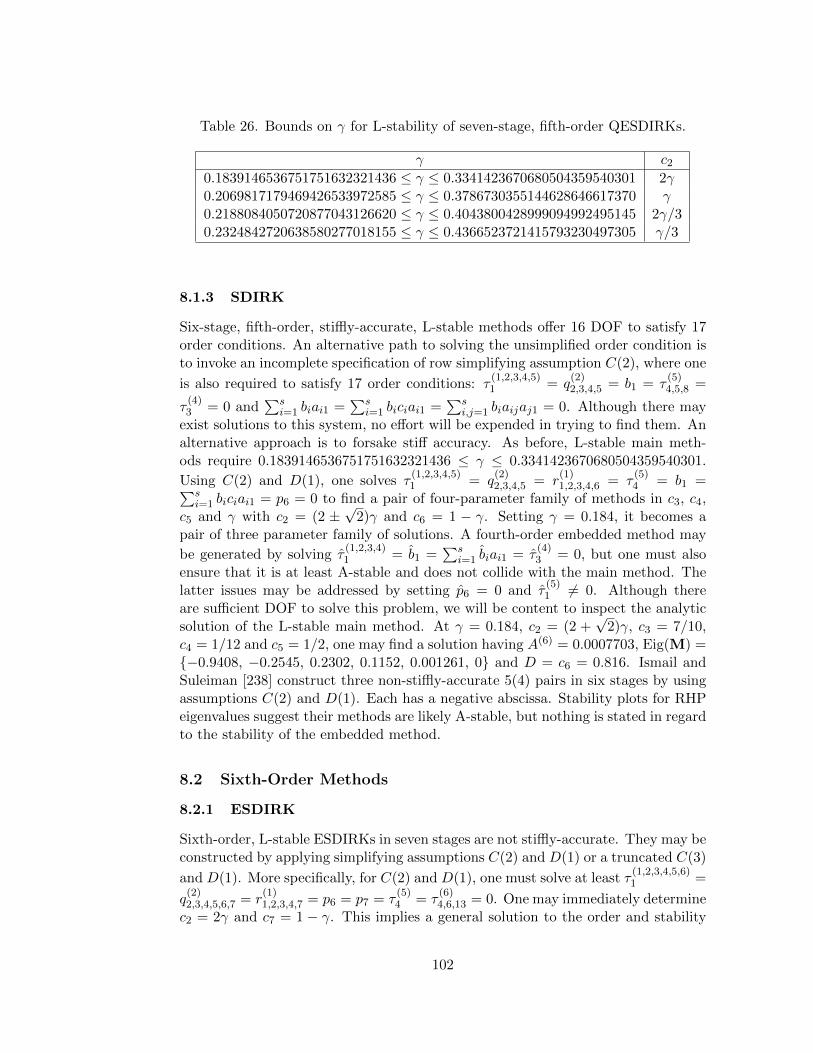
Table 26. Bounds on γ for L-stability of seven-stage, fifth-order QESDIRKs.
γ c2
0.1839146536751751632321436 ≤ γ ≤ 0.3341423670680504359540301 2γ0.2069817179469426533972585 ≤ γ ≤ 0.3786730355144628646617370 γ0.2188084050720877043126620 ≤ γ ≤ 0.4043800428999094992495145 2γ/30.2324842720638580277018155 ≤ γ ≤ 0.4366523721415793230497305 γ/3
8.1.3 SDIRK
Six-stage, fifth-order, stiffly-accurate, L-stable methods offer 16 DOF to satisfy 17order conditions. An alternative path to solving the unsimplified order condition isto invoke an incomplete specification of row simplifying assumption C(2), where one
is also required to satisfy 17 order conditions: τ(1,2,3,4,5)1 = q
(2)2,3,4,5 = b1 = τ
(5)4,5,8 =
τ(4)3 = 0 and
∑si=1 biai1 =
∑si=1 biciai1 =
∑si,j=1 biaijaj1 = 0. Although there may
exist solutions to this system, no effort will be expended in trying to find them. Analternative approach is to forsake stiff accuracy. As before, L-stable main meth-ods require 0.1839146536751751632321436 ≤ γ ≤ 0.3341423670680504359540301.
Using C(2) and D(1), one solves τ(1,2,3,4,5)1 = q
(2)2,3,4,5 = r
(1)1,2,3,4,6 = τ
(5)4 = b1 =∑s
i=1 biciai1 = p6 = 0 to find a pair of four-parameter family of methods in c3, c4,c5 and γ with c2 = (2 ±
√2)γ and c6 = 1 − γ. Setting γ = 0.184, it becomes a
pair of three parameter family of solutions. A fourth-order embedded method may
be generated by solving τ(1,2,3,4)1 = b1 =
∑si=1 biai1 = τ
(4)3 = 0, but one must also
ensure that it is at least A-stable and does not collide with the main method. Thelatter issues may be addressed by setting p6 = 0 and τ
(5)1 6= 0. Although there
are sufficient DOF to solve this problem, we will be content to inspect the analyticsolution of the L-stable main method. At γ = 0.184, c2 = (2 +
√2)γ, c3 = 7/10,
c4 = 1/12 and c5 = 1/2, one may find a solution having A(6) = 0.0007703, Eig(M) ={−0.9408, −0.2545, 0.2302, 0.1152, 0.001261, 0} and D = c6 = 0.816. Ismail andSuleiman [238] construct three non-stiffly-accurate 5(4) pairs in six stages by usingassumptions C(2) and D(1). Each has a negative abscissa. Stability plots for RHPeigenvalues suggest their methods are likely A-stable, but nothing is stated in regardto the stability of the embedded method.
8.2 Sixth-Order Methods
8.2.1 ESDIRK
Sixth-order, L-stable ESDIRKs in seven stages are not stiffly-accurate. They may beconstructed by applying simplifying assumptions C(2) and D(1) or a truncated C(3)
and D(1). More specifically, for C(2) and D(1), one must solve at least τ(1,2,3,4,5,6)1 =
q(2)2,3,4,5,6,7 = r
(1)1,2,3,4,7 = p6 = p7 = τ
(5)4 = τ
(6)4,6,13 = 0. One may immediately determine
c2 = 2γ and c7 = 1 − γ. This implies a general solution to the order and stability
102
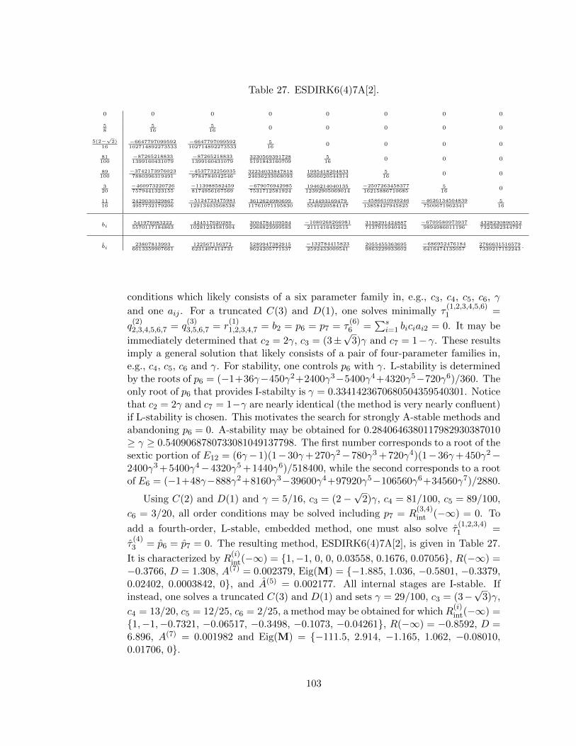
Table 27. ESDIRK6(4)7A[2].
0 0 0 0 0 0 0 0
58
516
516
0 0 0 0 0
5(2−√
2)16
−6647797099592102714892273533
−6647797099592102714892273533
516
0 0 0 0
81100
−872652188331399160431079
−872652188331399160431079
32305693917285191843160709
516
0 0 0
89100
−37421739760237880396319491
−45377322560359784784042546
3223403384781824636233068093
19954182048339606020544314
516
0 0
320
−4609732207267579441323155
−1139885824598174956167569
−6790769429857531712581924
194621404013512392905069014
−250726345837716215886710685
516
0
1116
24290303298674957732179206
−512472347598112913403568538
361262498069911761071195830
7144931694795549220584147
−458661094924613858427945825
−46261345048397500671962341
516
bi5419769832225570117184863
42451762028910281234581904
30047841095842968823999583
−10802682669812111416452515
31982914248877137915940442
−67095809739379894986011196
43282308905527324362344791
bi23807813993
66133599076611225671563726231407414731
52899473829159624205771537
−1327844158232592433009541
20554553636959863229933602
−6869524761846416474135057
27666315165797339217152243
.
conditions which likely consists of a six parameter family in, e.g., c3, c4, c5, c6, γ
and one aij . For a truncated C(3) and D(1), one solves minimally τ(1,2,3,4,5,6)1 =
q(2)2,3,4,5,6,7 = q
(3)3,5,6,7 = r
(1)1,2,3,4,7 = b2 = p6 = p7 = τ
(6)6 =
∑si=1 biciai2 = 0. It may be
immediately determined that c2 = 2γ, c3 = (3±√
3)γ and c7 = 1−γ. These resultsimply a general solution that likely consists of a pair of four-parameter families in,e.g., c4, c5, c6 and γ. For stability, one controls p6 with γ. L-stability is determinedby the roots of p6 = (−1+36γ−450γ2+2400γ3−5400γ4+4320γ5−720γ6)/360. Theonly root of p6 that provides I-stabilty is γ = 0.3341423670680504359540301. Noticethat c2 = 2γ and c7 = 1−γ are nearly identical (the method is very nearly confluent)if L-stability is chosen. This motivates the search for strongly A-stable methods andabandoning p6 = 0. A-stability may be obtained for 0.2840646380117982930387010≥ γ ≥ 0.5409068780733081049137798. The first number corresponds to a root of thesextic portion of E12 = (6γ−1)(1−30γ+ 270γ2−780γ3 + 720γ4)(1−36γ+ 450γ2−2400γ3 +5400γ4−4320γ5 +1440γ6)/518400, while the second corresponds to a rootof E6 = (−1+48γ−888γ2+8160γ3−39600γ4+97920γ5−106560γ6+34560γ7)/2880.
Using C(2) and D(1) and γ = 5/16, c3 = (2−√
2)γ, c4 = 81/100, c5 = 89/100,
c6 = 3/20, all order conditions may be solved including p7 = R(3,4)int (−∞) = 0. To
add a fourth-order, L-stable, embedded method, one must also solve τ(1,2,3,4)1 =
τ(4)3 = p6 = p7 = 0. The resulting method, ESDIRK6(4)7A[2], is given in Table 27.
It is characterized by R(i)int(−∞) = {1,−1, 0, 0, 0.03558, 0.1676, 0.07056}, R(−∞) =
−0.3766, D = 1.308, A(7) = 0.002379, Eig(M) = {−1.885, 1.036, −0.5801, −0.3379,0.02402, 0.0003842, 0}, and A(5) = 0.002177. All internal stages are I-stable. Ifinstead, one solves a truncated C(3) and D(1) and sets γ = 29/100, c3 = (3−
√3)γ,
c4 = 13/20, c5 = 12/25, c6 = 2/25, a method may be obtained for which R(i)int(−∞) =
{1,−1,−0.7321, −0.06517, −0.3498, −0.1073, −0.04261}, R(−∞) = −0.8592, D =6.896, A(7) = 0.001982 and Eig(M) = {−111.5, 2.914, −1.165, 1.062, −0.08010,0.01706, 0}.
103
8.2.2 DIRK
Using simplifying asumptions C(2) and D(2), Cooper and Sayfy [116] derive a sixth-order, A-stable DIRK in six stages with a11 = a22 = a33 = a44 = a55 = γ;however, the sixth stage is explicit (a66 = 0). Because of the assumptions used,
b1 = b2 = a66 = 0 and c6 = 1. Additionally, one enforces τ(1,2,3,4,5,6)1 = q
(2)3,4,5,6 =
r(1)1,2,3 = r
(2)1,2 = τ
(6)4,8 = E6 = 0. The system of equations has two solutions,
one of which is given by Cooper and Sayfy [116]. As part of this general solu-tion, one may derive c3 = (2 − 5c4 − 10γ + 20c4γ)/(5(1 − 4c4 − 4γ + 12c4γ)),
c4 =(5− 45γ + 80γ2±
√5(2− 36γ + 225γ2 − 560γ3 + 480γ4)
)/(5(3−24γ+40γ2)),
c5 = (1 − 2γ) and c6 = 1. A-stability is ensured by selecting the root of E6 =(−40 + 1200γ − 12000γ2 + 48000γ3 − 72000γ4 + 28800γ5)/14400 that provides I-stability; γ = 0.4732683912582953244555885. Cooper and Sayfy provide the minussolution with c2 = −6547598275475/ 14857672547324, D = 1.489, A(7) = 0.01238and Eig(M) = {0.656534, −0.282101, 0.238065, −0.0652908, 0, 0}. With posi-tive abscissae and one-third the error, the plus solution has c2 = 3496971800427/10494969937463, D = 17.82, A(7) = 0.004480 and Eig(M) = {3.0919, −2.89351,0.406624, −0.0578076, 0, 0}.
9 Seven- and Eight-stage Methods (SI = 7)
9.1 Fifth-Order Methods
9.1.1 ESDIRK
Eight-stage, stiffly-accurate, stage-order two ESDIRK methods with internal error-control
0 0 0 0 0 0 0 0 02γ γ γ 0 0 0 0 0 0c3 (c3 − a32 − γ) a32 γ 0 0 0 0 0c4 (c4 − a42 − a43 − γ) a42 a43 γ 0 0 0 0c5 (c5 − a52 − a53 − a54 − γ) a52 a53 a54 γ 0 0 0c6 (c6 − a62 − a63 − a64 − a65 − γ) a62 a63 a64 a65 γ 0 01 (1− a72 − a73 − a74 − a75 − a76 − γ) a72 a73 a74 a75 a76 γ 01 (1− b2 − b3 − b4 − b5 − b6 − b7 − γ) b2 b3 b4 b5 b6 b7 γ
bi (1− b2 − b3 − b4 − b5 − b6 − b7 − γ) b2 b3 b4 b5 b6 b7 γ
bi (1− b2 − b3 − b4 − b5 − b6 − b7 − b8) b2 b3 b4 b5 b6 b7 b8
(265)
provide 29 DOF. Three of these are quickly dispensed via C(2, 2) (a21 = γ), τ(1)1
(c7 = 1) and τ(1)1 (c8 = 1). Methods having both L-stable main and embedded
methods may be constructed by using C(2) or C(3) in truncated form. In the
former case, one must solve the 25 conditions τ(1,2,3,4,5)1 = q
(2)2,3,4,5,6,7 = p7 = τ
(4)3 =
τ(5)4,5,8 = τ
(1,3,4)1 = τ
(4)3 = p6 = R
(3,4,5,6)int (−∞) = 0. The resulting solution leaves, for
example, c4, c5, c6 and γ, but with no guarantee of I-stability for either the main or
104
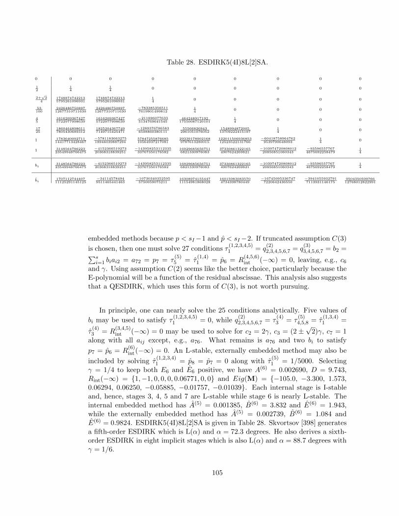
Table 28. ESDIRK5(4I)8L[2]SA.
0 0 0 0 0 0 0 0 0
12
14
14
0 0 0 0 0 0
2+√
24
17488747422135795261096931
17488747422135795261096931
14
0 0 0 0 0
53100
242648675089712677310711630
242648675089712677310711630
−7833853565117619901499812
14
0 0 0 0
45
16162093674275722977998639
16162093674275722977998639
−2118960776335134769641545
46424891719217550087120101
14
0 0 0
1725
18604648986117805430689312
18252043677497149715425471
−12893767865836598860380111
555668269432961051076052
154899487200513709222415197
14
0 0
1 178364009271114417713428467
−578118366327518946039887294
5784725587668510564937217081
293391789021689787613280015
12201150693685312523522131766
−604187589647629539790648093
14
0
1 314856478622323549948766475
−415236651927320368318839251
−14395825311233533767350176582
169296856567516821330976083
373308613221654907624269821
−10397472080801220856851060343
−935965577674675692258479
14
bi314856478622323549948766475
−415236651927320368318839251
−14395825311233533767350176582
169296856567516821330976083
373308613221654907624269821
−10397472080801220856851060343
−935965577674675692258479
14
bi170711274440711125291145125
−341145784949511465441463
−107303403525955750059075211
1630897415544711154981868028
160159830835704734398780449
−167450953367477220642436550
−39410559327917113931146175
950435059976612768012822991
embedded methods because p < sI−1 and p < sI−2. If truncated assumption C(3)
is chosen, then one must solve 27 conditions τ(1,2,3,4,5)1 = q
(2)2,3,4,5,6,7 = q
(3)3,4,5,6,7 = b2 =∑s
i=1 biai2 = a72 = p7 = τ(5)5 = τ
(1,4)1 = p6 = R
(4,5,6)int (−∞) = 0, leaving, e.g., c6
and γ. Using assumption C(2) seems like the better choice, particularly because theE-polynomial will be a function of the residual abscissae. This analysis also suggeststhat a QESDIRK, which uses this form of C(3), is not worth pursuing.
In principle, one can nearly solve the 25 conditions analytically. Five values of
bi may be used to satisfy τ(1,2,3,4,5)1 = 0, while q
(2)2,3,4,5,6,7 = τ
(4)3 = τ
(5)4,5,8 = τ
(1,3,4)1 =
τ(4)3 = R
(3,4,5)int (−∞) = 0 may be used to solve for c2 = 2γ, c3 = (2 ±
√2)γ, c7 = 1
along with all aij except, e.g., a76. What remains is a76 and two bi to satisfy
p7 = p6 = R(6)int (−∞) = 0. An L-stable, externally embedded method may also be
included by solving τ(1,2,3,4)1 = p8 = p7 = 0 along with τ
(5)1 = 1/5000. Selecting
γ = 1/4 to keep both E6 and E6 positive, we have A(6) = 0.002690, D = 9.743,Rint(−∞) = {1,−1, 0, 0, 0, 0.06771, 0, 0} and Eig(M) = {−105.0, −3.300, 1.573,0.06294, 0.06250, −0.05885, −0.01757, −0.01039}. Each internal stage is I-stableand, hence, stages 3, 4, 5 and 7 are L-stable while stage 6 is nearly L-stable. Theinternal embedded method has A(5) = 0.001385, B(6) = 3.832 and E(6) = 1.943,while the externally embedded method has A(5) = 0.002739, B(6) = 1.084 andE(6) = 0.9824. ESDIRK5(4I)8L[2]SA is given in Table 28. Skvortsov [398] generatesa fifth-order ESDIRK which is L(α) and α = 72.3 degrees. He also derives a sixth-order ESDIRK in eight implicit stages which is also L(α) and α = 88.7 degrees withγ = 1/6.
105
10 Test Problems
Testing of schemes is conducted on three singular perturbation problems: Kaps’problem, van der Pol’s equation and the Pareschi and Russo problem. The equationsexhibit increasing stiffness as ε→ 0 and, in the limit of ε = 0, the systems becomedifferential algebraic equation systems. Outside of singular perturbation problems,other simple test equations for stiff problems may be found in the literature [143,193, 288, 336, 378]. Anyone testing using the DETEST problem set should consultcomments made by Shampine [374].
The first singular perturbation problem considered is Kaps’ problem [129]
y1(t) = −(ε−1 + 2
)y1(t) + ε−1y2
2(t), y2(t) = y1(t)− y2(t)− y22(t), (266)
where 0 ≤ t ≤ 1 and whose exact solution is y1(t) = y22(t), y2(t) = exp(−t).
Equilibrium (unperturbed) initial conditions (ICs) are given by y1(0) = y2(0) = 1.In the limit of ε = 0, the system becomes an index-1 differential algebraic equationsystem.
Van der Pol’s (vdP) equation [190,193], the second problem, is given by,
y1(t) = y2(t), y2(t) = ε−1((1− y1(t)2)y2(t)− y1(t)
). (267)
Unperturbed ICs are given by [172, 193] y1(0) = 2, y2(0) = −2/3 + 10ε/81 −292ε2/2187 − 1814ε3/19683 + · · · . In the limit of ε = 0, the system becomes anindex-1 differential algebraic equation system. At large ε, this series expansionfails. However, nonequilibrium ICs will be specified for this equation by using thisexpansion and large values of ε.
Pareschi and Russo [336] have constructed a simple singular perturbation equa-tion
y1(t) = −y2(t), y2(t) = y1(t) + ε−1 (sin(y1(t))− y2(t)) . (268)
Equilibrium ICs are y1(0) = π/2, y2(0) = 1. Nonequilibrium, or perturbed, datamay be specified by replacing the condition on y2 with y2(0) = 1/2. Further compar-isions between integration methods including DIRK-type schemes are available inthe literature. In comparisons with other popular schemes, Hairer and Wanner [193]find the performance of the stage-order one SDIRK4 disappointing. This promptedCash [100] not even to include SDIRK methods in his stiff solver comparison. How-ever, comparisons conducted by Gaffney [161] and Sandu et al. [353] cast SDIRKmethods in a more favorable light. With Navier-Stokes applications in mind, Bijlet al. [38,39] show that ESDIRK schemes outperform SDIRK and BDF-methods insimulating laminar flows over airfoils and in complex multi-disciplinary flows involv-ing fluid-structure interactions. Jothiprasad et al. [248] conduct a similar study byfocusing particular attention on solution procedures for the coupled nonlinear stageand step equations. Carpenter et al. [93, 94] compare ESDIRK, BDF and MEBDFmethods on flows over airfoils by using moderately stiff turbulence models. Theyfind that ESDIRK methods are accurate even with very large timesteps, but oftenbecome decreasingly efficient in that limit. This inefficiency can result primarily
106
from dramatic slowdown of the algebraic equation solver. A partial remedy wouldbe the development of effective stage-value-predictors, so that ESDIRKs do notspend inordinate amounts of time converging stage and step iterations. Clemenset al. [108] compare a 3(2) SDIRK and Rosenbrock pair while solving nonlinearequations associated with magnetic fields. Conclusions from all of these tests needto be made while considering leading-order error of the methods, stage-order, localintegration error tolerance, equation stiffness and stage-value prediction techniques.
11 Discussion
After having thoroughly investigated matters relevant to the construction of usefuland efficient, general purpose, DIRK-type methods in §2, we now set about the taskof testing 29 methods. The goal of the testing is to establish whether methods areappropriate for general purpose settings and are free of substantial shortcomings, aswell as to determine the value of specific method characteristics. Less focus is placedon establishing whether one method is ”better” than another. Fifteen proposed newand existing DIRK-type methods: ESDIRK2(1)3L[2]SA, ESDIRK3(2)4L[2]SA, ES-DIRK3(2I)4L[2]SA, ESDIRK3(2)5L[2]SA, ESDIRK3(2I)5L[2]SA, ESDIRK4(3)5L-[2]SA, ESDIRK4(3I)5L[2]SA, ESDIRK4(3)6L[2]SA, ESDIRK4(3)6L[2]SA C(3), ES-DIRK4(3I)6L[2]SA, QESDIRK4(3)6L[2]SA, ESDIRK5(3)6L[2]SA, ESDIRK5(4)7L-[2]SA, ESDIRK5(4I)8L[2]SA and ESDIRK6(4)7A[2], are considered (see appendixC) along with 14 others: SDIRK2(1)2A[1]Alg, ESDIRK4(3)6L[2]SA A,B,C,D,E, ES-DIRK3(2)5L[2]SA SOD, ESDIRK4(3)6L[2]SA SOD, QESDIRK4(3)6L[2]SA SOD, ES-DIRK4(3)6L[2]SA ARK, SDIRK4(3)5L[1]SA C(2), QSDIRK4(3)5L[1]SA, SDIRK4(1)and SDIRK4(2). Most of these 14 additional methods are constructed to help assesscertain scheme attributes rather than to generate useful methods. Ideally, testingwill serve to confirm or refute predictions on scheme behavior, illuminate methodshortcomings, and allow the investigation of subtle changes in scheme design. Meth-ods ESDIRK3(2)5L[2]SA SOD, ESDIRK4(3)6L[2]SA SOD and QESDIRK4(3)6L-[2]SA SOD, are included to assess the value of stiff accuracy. Second-order damped,
L-stable methods when q(3)3,4,··· ,(s−1) = 0 is imposed. No SOD methods are con-
structed without imposing q(3)3,4,··· ,(s−1) = 0. Also included is the implicit por-
tion of ARK4(3)6L[2]SA [255], named ESDIRK4(3)6L[2]SA ARK for reference pur-poses. Consequences of nonvanishing values of the internal stability function forlarge eigenvalues on intermediate stages (3,4 and 5) are investigated using the fivestiffly-accurate, L-stable, stage-order 2 methods characterized in Table 18: ES-DIRK4(3)6L[2]SA A,B,C,D,E. To assess the potential of DIRK-type methods witha11 6= 0, stiff accuracy, L-stability and a stage-order of one, both SDIRK meth-ods proposed by Hairer and Wanner [193], SDIRK4(1) and SDIRK4(2), are in-
cluded along with two methods using q(2)2,3,4 = 0: SDIRK4(3)5L[1]SA C(2) and QS-
DIRK4(3)5L[1]SA. The last method, SDIRK2(1)2A[1]Alg, is chosen to compare analgebraically stable, strongly regular method to the stiffly- accurate, L-stable methodESDIRK2(1)3L[2]SA.
It should be kept in mind that one very important aspect of these methods has
107
been largely forsaken: stage-value predictors. A thorough investigation of construc-tion choices and of testing the best approaches to stage-value predictor design is avery large undertaking beyond the scope of this paper. We shall be content withthe analysis provided in §2.18. However, one should expect that higher stage-order,as well as good internal stability, will facilitate quality predictors. No testing isconducted on discontinuities. Due to the very large number of graphs that wouldbe required to support a thorough examination of each scheme’s behavior on allperformance attributes considered, a strictly verbal description follows.
11.1 Convergence
All convergence tests are done using the three singular perturbation test problems,with the same ICs for each test problem, and integrating them over the same timeinterval. Step-sizes are held constant. Singular perturbation problems are very use-ful for detecting shortcomings of methods but may not be particularly illuminatingat distinguishing which well designed method is more accurate in practical set-tings. They also fail to exercise many important implementation matters. For thesereasons, we will be content to offer qualitative assessments of scheme convergenceperformance rather than quantifying performance in such simple settings.
11.1.1 Second-Order Methods
The two second-order methods tested in this paper were ESDIRK2(1)3L[2]SA andSDIRK2(1)2A[1]Alg. In terms of leading order accuracy, SDIRK2(1)2A[1]Alg ismore accurate with A(3) = 0.02329 versus A(3) = 0.05719. Method ESDIRK2(1)3L-[2]SA is stiffly-accurate, L-stable and has a stage-order of 2. In contrast, SDIRK-2(1)2A[1]Alg is algebraically stable but not L-stable or stiffly-accurate, has a stage-order of 1 and is strongly regular. Each has a similar value of γ (0.2500 versus≈ 0.2929). Since the second stage of ESDIRK2(1)3L[2]SA is essentially a shortenedTrapezoidal rule, the stage is neutrally stable to stiff eigenvalues.
At ε = 0, the SDIRK is predictably more accurate than the ESDIRK on the vdPequation. As stiffness increases, each method behaves differently. For the SDIRK,the differential variable becomes more accurate while retaining second order accu-racy. However, the algebraic variable becomes substantially less accurate, its orderreduces slightly and it has a rather erratic convergence behavior at ε = 10−3. Con-vergence behavior of the ESDIRK is smoother, suffers from no order reduction anddoes not experience as large an increase in algebraic variable error as stiffness is ap-plied. For very large step-sizes, the convergence behavior of the ESDIRK is erratic.On Kaps’ and the Pareschi and Russo problem, stiffness increases have less of aninfluence on the methods than when solving the vdP equation. SDIRK2(1)2A[1]Algstill has more difficulty with the algebraic variable. This is made dramatically ap-parent using nonequilibrium ICs on the Pareschi and Russo problem. Stage-order 2plus L-stability seems to be more useful than stage-order 1 plus algebraic stabilityand strong regularity when solving stiff problems, particularly with nonequilibriumICs.
108
11.1.2 Third-Order Methods
Five third-order methods have been tested: ESDIRK3(2)4L[2]SA, ESDIRK3(2I)4L-[2]SA, ESDIRK3(2)5L[2]SA, ESDIRK3(2I)5L[2]SA and ESDIRK3(2)5L[2]SA SOD.Each method is L-stable, stiffly-accurate and has a stage order of 2. Method
ESDIRK3(2)5L[2]SA SOD is different from the others in that it invokes q(3)3,4 = 0
and has a second-order damped stability function. The four-stage methods are
both characterized by γ ≈ 0.4359 and have R(3)int = −0.8057, (−0.9567) and A(4) =
0.03663, (0.4907) for the method without (with) internal error-control. Similarly, for
the five stage methods without SOD, γ = 0.225 and have R(3,4)int = 0, 0, (17/81, 0)
and A(4) = 0.0007769, (0.01149) for the method without (with) internal error-
control. ESDIRK3(2)5L[2]SA SOD has γ ≈ 0.3025, R(3,4)int = {(1 −
√3), 0} and
A(4) = 0.01806.
The behavior of third-order methods strongly depends on whether one is solvingthe difficult vdP equation, the easier Kaps’ problem, or the even milder Pareschiand Russo problem. In the most severe circumstances, solving the vdP equation,ESDIRK3(2)5L[2]SA and ESDIRK3(2I)5L[2]SA are decidedly better performingmethods than the others. ESDIRK3(2)5L[2]SA SOD has severe solvability problemsthat render it rather useless at stiffness levels of ε ≤ 10−3. Both ESDIRK3(2)4L-[2]SA and ESDIRK3(2I)4L[2]SA methods suffer from solvability problems at largerstep-sizes and ε ≤ 10−3. Between ESDIRK3(2)5L[2]SA and ESDIRK3(2I)5L[2]SA,internal error control is obtained at a substantial accuracy penalty as ESDIRK-3(2)5L[2]SA is decidedly more accurate. Also, ESDIRK3(2)5L[2]SA appears to su-perconverge, to order p+ 1, at large time steps for the differential variable. None ofthe other 3(2) pairs exhibits superconvergence. Order reduction of each of the five3(2) pairs is modest and is generally confined to the algebraic variable. On the easierproblems, order reduction was nearly nonexistent except for ESDIRK3(2I)5L[2]SAon Kaps’s problem at ε = 10−3. All methods converge at essentially third-order,independent of stiffness. ESDIRK3(2)5L[2]SA exhibits superconvergence on thePareschi and Russo problem at large step sizes. The most obvious difference be-tween methods that do or do not have internal error-control is the performance ofthe algebraic variable, but this difference is not manifested consistently. MethodsESDIRK3(2I)5L[2]SA and ESDIRK3(2)4L[2]SA have more erratic convergence oftheir algebraic variables. This may suggest that something other than the internalerror-control, and the attendant confluent abscissae, is influencing matters. Of allfive 3(2) pairs, only ESDIRK3(2)5L[2]SA SOD cannot be recommended. Redesign-
ing it without invoking q(3)3,4 = 0 might make for better SOD methods.
11.1.3 Fourth-Order Methods
Eighteen of the 29 methods tested in this paper are L-stable, stiffly-accurate, fourth-order methods: ESDIRK4(3)5L[2]SA, ESDIRK4(3I)5L[2]SA, ESDIRK4(3)6L[2]SA,ESDIRK4(3)6L[2]SA C(3), ESDIRK4(3I)6L[2]SA, QESDIRK4(3)6L[2]SA, ESDIRK-4(3)6L[2]SA A,B,C,D,E, ESDIRK4(3)6L[2]SA SOD, QESDIRK4(3)6L[2]SA SOD, ES-DIRK4(3)6L[2]SA ARK, SDIRK4(3)5L[1]SA C(2), QSDIRK4(3)5L[1]SA, SDIRK-
109
4(1) and SDIRK4(2). Fourteen are stage-order two (Q)ESDIRKs and four arestage-order one (Q)SDIRKs. Twelve of the 18 methods have γ = 1/4.
To test stage-order one methods, the two SDIRK4 methods of Hairer and Wan-
ner [193] are used as well as two methods employing q(2)2,3,4 = 0: SDIRK4(3)5L-
[1]SA C(2) and QSDIRK4(3)5L[1]SA. These four methods have γ = 1/4, exceptQSDIRK4(3)5L[1]SA where γ = 8/25. Leading order errors for the methods SDIRK-4(1), SDIRK4(2), SDIRK4(3)5L[1]SA C(2) and QSDIRK4(3)5L[1]SA are A(5) =0.002504, 0.004229, 0.002454, 0.006849, respectively. Amongst the 14 stage-ordertwo methods with a11 = 0, two are five-stage methods: ESDIRK4(3)5L[2]SA and
ESDIRK4(3I)5L[2]SA. Both have γ ≈ 0.5728 and nonzero values of R(3,4)int (−∞).
Leading order errors for these two methods, A(5) = 0.03857(0.04506) for the methodwithout (with) interior error control, with four implicit stages, are often substan-tially higher than the remaining 12 stage-order two methods with five implicit stages.Two of the methods are QESDIRKs with a22 = γ/3, γ = 0.3200 (QESDIRK-
4(3)6L[2]SA), and γ ≈ 0.4803 (QESDIRK4(3)6L[2]SA SOD), q(3)3,4,5 = 0, and each
with the relatively large values of A(5) = 0.004828 and A(5) = 0.05848, respec-tively. Two of the methods have second order damped stability functions withγ ≈ 0.3889 (ESDIRK4(3)6L[2]SA SOD with A(5) = 0.01670) and γ ≈ 0.4803
(QESDIRK4(3)6L[2]SA SOD), along with q(3)3,4,5 = 0. Five methods modeled after
ESDIRK4(3)6L[2]SA, ESDIRK4(3)6L[2]SA A,B,C,D,E, are used to test the conse-
quences of setting∣∣∣R(3,4,5)
int (−∞)∣∣∣ = n/2 where n = 1, 2, · · · , 5. All have similar
leading order errors (See Table 18). Two methods are constructed with both inter-nal and external error-control, ESDIRK4(3I)5L[2]SA and ESDIRK4(3I)6L [2]SA,and may be compared against their similar and more traditional analogs, ESDIRK-4(3)5L[2]SA and ESDIRK4(3)6L[2]SA. Leading order error for the four methodsis A(5) = 0.04506, 0.002254, 0.03857, 0.001830, respectively. Methods ESDIRK-4(3)6L[2]SA (A(5) = 0.001830), ESDIRK4(3)6L[2]SA ARK (A(5) = 0.003401) andESDIRK4(3)6L[2]SA C(3) (A(5) = 0.002970) are each straightforward methods thatcould potentially be applied widely. While each is stage-order two, ESDIRK4(3)6L-
[2]SA C(3) also satisfies q(3)3,4,5 = 0. Both ESDIRK4(3)6L[2]SA and ESDIRK4(3)6L-
[2]SA C(3) have fully damped internal stability functions at stages where this ispossible.
Beginning with the easiest problem, no discernable order reduction is seen forany of the stage-order two methods on the Pareschi and Russo problem with equi-librium ICs. Order reduction in stage-order one methods was mild and occured
at very tight tolerances with ε = 10−3. Use of q(2)2,3,4 = 0 appeared to mildly mit-
igate order reduction on the stage-order one methods. Methods ESDIRK4(3)6L-[2]SA A,B,C,D,E applied using nonequilibrium ICs showed worse behavior of thealgebraic variable relative to ESDIRK4(3)6L[2]SA and other stage-order two meth-ods. Nonequilibrium ICs induce order reduction of the algebraic variable at smallstep-sizes on all methods. QESDIRK4(3)6L[2]SA had the most accurate algebraic
variable at moderate to large step sizes. (Q)SDIRK methods using q(2)2,3,4 = 0 had
less erratic convergence behavior of the algebraic variable at ε = 10−3 and small
110
step-sizes than the other stage-order one methods. Order reduction for all meth-ods was mild, and little difference existed between stage-order two and stage-orderone methods. All in all, the Pareschi and Russo problem is not terribly demand-ing of the integration method. For Kaps’ problem, order reduction is more pro-nounced at ε = 10−3 than it is on the Pareschi and Russo problem. Schemes usedto test the effects of internal instability, ESDIRK4(3)6L[2]SA A,B,C,D,E, have er-ratic convergence rates of the algebraic variable that grow increasingly erratic at
small step-sizes and as n increases with∣∣∣R(3,4,5)
int (−∞)∣∣∣ = n/2, n = 1, 2, · · · , 5.
QESDIRK4(3)6L[2]SA appears to offer no advantage over ESDIRK4(3)6L[2]SA on
Kaps’ problem. Adding a truncated version of assumption C(3) in the form q(3)3,4,5 = 0
with ESDIRK4(3)6L[2]SA C(3) also offers no benefit. QSDIRK4(3)5L[1]SA clearlyimproves algebraic variable error at large step sizes over SDIRK(1), SDIRK(2) andSDIRK4(3)5L[1]SA C(2). Stage-order two methods have dramatically better al-gebraic variable error at ε = 10−3 than stage-order one methods. This also ap-plies to ε = 10−6 at small step sizes. On the most difficult problem, the vdPequation, QESDIRK4(3)6L[2]SA has slightly better algebraic variable error thanESDIRK4(3)6L[2]SA at lax error tolerances. Otherwise, methods ESDIRK4(3)5L-[2]SA, ESDIRK4(3I)5L[2]SA, ESDIRK4(3)6L[2]SA, ESDIRK4(3)6L[2]SA C(3), ES-DIRK4(3I)6L[2]SA, QESDIRK4(3)6L[2]SA and ESDIRK4(3)6L[2]SA ARK behavesimilarly. Internal stability testing methods, ESDIRK4(3)6L[2]SA A,C,D,E, havesignificant solvability shortcomings. As with Kaps’ problem, stage-order two meth-ods perform much better on their algebraic variables than stage-order one methods.Both SOD methods perform badly. Again, adding a truncated version of assumption
C(3) with ESDIRK4(3)6L[2]SA C(3) in the form q(3)3,4,5 = 0 also offers no discernable
benefit.
11.1.4 Fifth- and Sixth-Order Methods
Convergence rate testing of higher-order ESDIRKs involves three fifth-order meth-ods: ESDIRK5(3)6L[2]SA, ESDIRK5(4)7L[2]SA, ESDIRK5(4I)8L[2]SA and one sixth-order method: ESDIRK6(4)7A[2]. All methods are stage-order two, but only thefifth-order methods are stiffly-accurate and L-stable. The sixth-order method isstrongly A-stable. Values of γ and A(6) for the fifth-order methods are γ ≈ 0.2781,0.1840, 0.2500, and A(6) = 0.004615, 0.001846, 0.002690, respectively. For ESDIRK-6(4)7A[2], γ = 0.3125, R(−∞) = −0.3766, and A(7) = 0.002379. For stages 3, 4, 5and 6, only ESDIRK5(3)6L[2]SA is not fully damped in the far LHP.
As expected, the performance of each method is very good on the rather benignPareschi and Russo problem. Order reduction becomes noticable with Kaps’ prob-lem and pronounced with the vdP equation. Beginning with the Pareschi and Russoproblem, order reduction with equilibrium ICs occurs principally around ε ≈ 10−3
and at moderate to small step-sizes but not large step-sizes. On error versus step-sizeplots, in order of decreasing accuracy, ESDIRK6(4)7A[2] > ESDIRK5(4)7L[2]SA> ESDIRK5(3)6L[2]SA > ESDIRK5(4I)8L[2]SA. Switching to nonequilibrium ICsdramatically increases the algebraic variable error and order-reduction, particularlynear ε ≈ 10−3. In spite of not being stiffly-accurate or L-stable, ESDIRK6(4)7A[2]
111
is still quite accurate. Methods ESDIRK5(4)7L[2]SA and ESDIRK5(3)6L[2]SA be-have similarly, but ESDIRK5(4I)8L[2]SA is less accurate than either. Kaps’ problemis severe enough to cause the algebraic variable error in method ESDIRK6(4)7A[2]to seriously degrade with increasing stiffness rather than simply near ε ≈ 10−3.However, the differential variable is still resolved better with this method than theother three methods. Methods ESDIRK5(4)7L[2]SA and ESDIRK5(3)6L[2]SA areof similar accuracy, but ESDIRK5(4)7L[2]SA is more accurate for very stiff modeswhile each is more accurate than ESDIRK5(4I)8L[2]SA. Solvability problems associ-ated with ESDIRK5(3)6L[2]SA on the vdP equation at stiffnesses ε ≤ 10−3 make itsuse inadvisable on such nasty problems. Both ESDIRK5(4)7L[2]SA and ESDIRK-5(4I)8L[2]SA work relatively well, with the former being more accurate. WithoutL-stability and stiff accuracy, ESDIRK6(4)7A[2] not only has a very inaccurate al-gebraic variable for nontrivial stiffnesses, it also loses accuracy in the differentialvariable at ε ≈ 10−3. It is an interesting question to ask how much the lack ofinternal I-stability on stage 6 influenced the performance of ESDIRK5(4)7L[2]SAon these tests.
11.2 Solvability
Generally, the maximum step-size possible with a DIRK-type method is given byν(∆t) < Min (aii)
−1. Beyond this value of (∆t), one is no longer assured a uniquesolution to the coupled nonlinear stage and step equations. This relation impliesthat reduced values of aii enable larger maximum step-sizes. However, testing ofthe many methods shows that this maximum step-size depends on more than ν andaii. While no attempt was made to compute ν and compare results to the expres-sion ν(∆t) < Min (aii)
−1, one may look into whether stiffness has any affect on themaximum step-size. This stiffness dependence only becomes clearly apparent whenmethods are tested on the more severe vdP equation but not on Kaps’ problem orPareschi and Russo’s problem. However, no investigation is made about solvabilitybehavior on large systems of equations. Small anomalies occur on Kaps’ problem for10−1 ≤ ε ≤ 100 with several methods. Switching from equilibrium to nonequilibriumICs on Pareschi and Russo’s problem has no noticable affect. By solving the vdPequation, one may place the 29 methods into one of three categories: essentially unaf-fected, moderately affected and severely affected. Thirteen of the 29 were essentiallyor totally unaffected: SDIRK2(1)2A[1]Alg, ESDIRK3(2)5L[2]SA, ESDIRK3(2I)5L-[2]SA, ESDIRK4(3I)5L[2]SA, ESDIRK4(3)6L[2]SA, ESDIRK4(3)6L[2]SA C(3), ES-DIRK4(3I)6L[2]SA, QESDIRK4(3)6L[2]SA, ESDIRK4(3)6L[2]SA ARK,SDIRK4(3)5L[1]SA C(2), QSDIRK4(3)5L[1]SA, ESDIRK5(4I)8L[2]SA and ESDIRK-6(4)7A[2]. Those methods that were moderately affected are: ESDIRK2(1)3L[2]SA,ESDIRK3(2)4L[2]SA, ESDIRK3(2I)4L[2]SA, ESDIRK4(3)5L[2]SA, ESDIRK5(4)7L-[2]SA, ESDIRK4(3)6L[2]SA SOD and ESDIRK4(3)6L[2]SA B. Methods whose max-imum step-size was strongly affected by stiffness are: ESDIRK4(3)6L[2]SA A,C,D,E,ESDIRK3(2)5L[2]SA SOD, QESDIRK4(3)6L[2]SA SOD, ESDIRK5(3)6L[2]SA, S-DIRK4(1) and SDIRK4(2). It is not obvious why certain methods behaved differ-ently from others in this test. Of the five methods designed specifically to investigate
112
the affects of internal instability, four of them were severely affected by stiffness whilethe fifth was only moderately affected. We tentatively conclude that internal stabil-ity is an important attribute to possess for solvability. Note that each of these five
methods controls R(i)int(−∞), i = 3, 4, 5 but not R
(i)int(z), i = 3, 4, 5. Methods having
second-order damped, L-stability fared poorly on this test. One may speculate that
the highly constrained second-order damped methods with q(3)3,4,··· ,(s−1) = 0 possessed
poor internal stability away from z = −∞. This hypothesis is not actually investi-
gated. As method ESDIRK5(3)6L[2]SA has nonzero values of R(i)int(−∞), i = 3, 4, 5,
it is also suspected that poor performance of the method is caused by insufficientdamping of stiff modes in the internal stages. Lastly, the behavior of the four fourth-order (Q)SDIRK methods seemed to depend on whether they were designed using
simplifying assumption C(2) in the truncated form q(2)2,3,4 = 0. Methods SDIRK-
4(3)5L[1]SA C(2) and QSDIRK4(3)5L[1]SA behaved much better than SDIRK4(1)and SDIRK4(2) on this solvability test. While internal stability is not ruled out,it appears that an incomplete specification of assumption C(2) benefits stage-orderone methods.
11.3 Error Estimation and Step-Size Control
Step-size selection based on an error estimate from an embedded method and anerror controller, but not in conjunction with iteration control, is tested on the threetest problems with both equilibrium and nonequilibrium initial conditions. Ideally,the error controller delivers a local error nearly equal to the error tolerance alongwith a smooth step-size sequence. As there are 27 p(p − 1) pairs being tested andnumerous error-controllers available, the first test is to see how each method be-haves with the established controllers: I, H211, PC, PID, H312, PPID, H321, H0321and H0330. Each method with each controller is used to solve the vdP equationon the same time interval using equilibrium ICs and ε = 10−5. Methods havingstage-order one and a11 6= 0 were all rather insensitive to the controller choice anddelivered an error slightly larger than the requested error. Among these methods,
imposing q(2)i = 0, i = 2, 3, 4 modestly improved the ability of the controllers to
deliver the requested error tolerance. It should be noted that the embedded meth-ods used with SDIRK4(1) and SDIRK4(2) were the revised A-stable methods andnot the original methods. Stage-order two ESDIRKs and QESDIRKs behaved quitedifferently. Their delivered local error, relative to the requested error, was stronglydependent on the controller choice. From the published controllers, ESDIRKs andQESDIRKs worked well with only the PPID and H321 controllers. Each is fromthe class of controllers having third-order dynamics, second-order adaptivity andfirst-order filtering but having different roots to the characteristic polynomial. Ex-panding to H0pDpApF controllers having pD = pA + pF and pD = 4, 5 producedno useful controllers for these methods on the vdP equation. It would seem thatnonzero roots to the controller are essential for good behavior in this context. Thismay explain why H312, which has the roots (0, 0, 1/2), did not perform well. Thenext test also uses the vdP equation with equilibrium ICs but uses only methodESDIRK4(3)6L[2]SA. Both H321general and H312general controllers are investigated
113
to find the affect of the characteristic root placement. The behavior of the con-trollers is strongly influenced by root placement. Several roots were found during acoarse search, which provide a high-quality error controller for both H321general andH312general with ESDIRK4(3)6L[2]SA: (q1, q2, q3) = (−0.5, 0.7, 0.8), (0.3, 0.3, 0.8),(0.4, 0.5, 0.6), (0.4, 0.5, 0.7) and (0.6, 0.6, 0.6). Again, H321 and PPID have rootsgiven by {1/3, 1/2, 2/3} and {0.4838± 0.3275I, 0.7325}, respectively. Roots havingcomplex conjugate pairs were not investigated. It appears that good controllershaving only real roots have roots −0.5 ≤ qi ≤ 0.8. Further tests showed that anH321general or H312general controller with ESDIRK4(3)6L[2]SA that worked well onthe vdP equation having equilibrium ICs also worked well on the other test prob-lems, including those with nonequilibrium ICs. However, controllers that workedwell with one ESDIRK could behave poorly with a different ESDIRK. The abilityof any H321general or H312general controller to deliver the requested error toleranceis often similar, given the same roots to the characteristic polynomial of the con-trollers. For the ESDIRKs and QESDIRKs, the controllers seem to be sensitiveto the method but not the problem. This is not due to matters such as internalstability. Embedded method construction is guided by parameters defining a goodembedded method for an ERK. It is possible that the parameters, B(p+2), C(p+2)
and E(p+2), (29), should be carefully chosen using different criteria or that anotherparameter is needed for the design of ESDIRK and QESDIRK embedded methods.The uniform lack of sensitivity of SDIRK and QSDIRK methods to controller choiceis puzzling in view of the consistent sensitivity of the ESDIRK and QESDIRK tocontroller choice (using externally or internally embedded methods).
Another attribute of a good controller is that it minimizes the work requiredto complete an integration by not prompting rejected steps. Controllers that con-sistently delivered an error that is significantly larger than the requested error areprone to have large numbers of rejected steps and are very inefficient at deliveringaccurate solutions. All of the good controllers yield similar efficiency on the vdPequation over the entire spectrum of target errors. A common technique in dealingwith a rejected step is to simply halve (or some other factor) the step-size and be-gin the step again. Doing this rather than computing a new step-size that woulddeliver the requested error based on the order of the method could interfere withthe operation of the error controller and might best be avoided. The delivered erroron the vdP equation at large step-sizes was very erratic for the ESDIRK schemes.This was partially attributable to rounding error.
Tests using ESDIRK methods that possess both internally and externally em-bedded methods, show similar results in all situations. For the methods presentedin this paper applied to stiff ODEs, it would seem unlikely that the methods havinginternally embedded methods offer any tangible benefit over traditional methods.However, no attempt was made to utilize both simultaneously for something likestiffness estimation or order reduction detection.
It is sometimes remarked that an SDIRK has an advantage over an ESDIRKwhen the ICs to the step are effectively nonequilibrium because the ESDIRK in-corporates the function evaluation of this IC into future values of the integrationvariable [246]. ESDIRK and QESDIRK methods designed in this paper did not
114
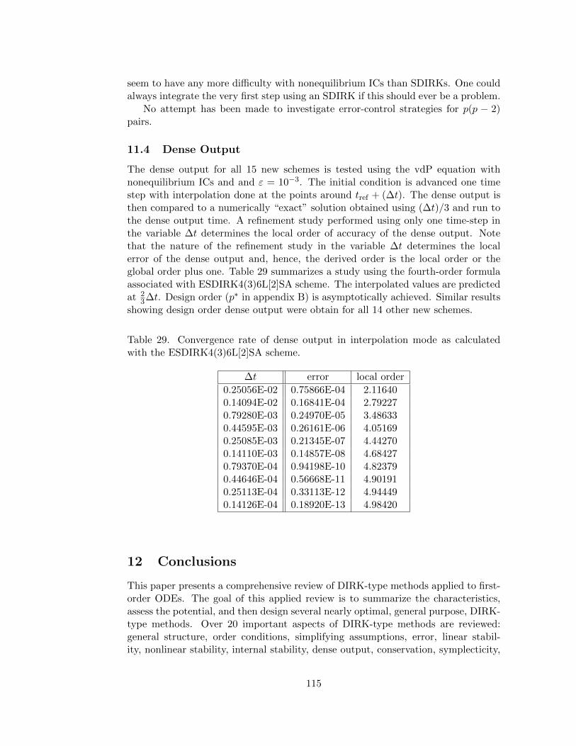
seem to have any more difficulty with nonequilibrium ICs than SDIRKs. One couldalways integrate the very first step using an SDIRK if this should ever be a problem.
No attempt has been made to investigate error-control strategies for p(p − 2)pairs.
11.4 Dense Output
The dense output for all 15 new schemes is tested using the vdP equation withnonequilibrium ICs and and ε = 10−3. The initial condition is advanced one timestep with interpolation done at the points around tref + (∆t). The dense output isthen compared to a numerically “exact” solution obtained using (∆t)/3 and run tothe dense output time. A refinement study performed using only one time-step inthe variable ∆t determines the local order of accuracy of the dense output. Notethat the nature of the refinement study in the variable ∆t determines the localerror of the dense output and, hence, the derived order is the local order or theglobal order plus one. Table 29 summarizes a study using the fourth-order formulaassociated with ESDIRK4(3)6L[2]SA scheme. The interpolated values are predictedat 2
3∆t. Design order (p∗ in appendix B) is asymptotically achieved. Similar resultsshowing design order dense output were obtain for all 14 other new schemes.
Table 29. Convergence rate of dense output in interpolation mode as calculatedwith the ESDIRK4(3)6L[2]SA scheme.
∆t error local order
0.25056E-02 0.75866E-04 2.116400.14094E-02 0.16841E-04 2.792270.79280E-03 0.24970E-05 3.486330.44595E-03 0.26161E-06 4.051690.25085E-03 0.21345E-07 4.442700.14110E-03 0.14857E-08 4.684270.79370E-04 0.94198E-10 4.823790.44646E-04 0.56668E-11 4.901910.25113E-04 0.33113E-12 4.944490.14126E-04 0.18920E-13 4.98420
12 Conclusions
This paper presents a comprehensive review of DIRK-type methods applied to first-order ODEs. The goal of this applied review is to summarize the characteristics,assess the potential, and then design several nearly optimal, general purpose, DIRK-type methods. Over 20 important aspects of DIRK-type methods are reviewed:general structure, order conditions, simplifying assumptions, error, linear stabil-ity, nonlinear stability, internal stability, dense output, conservation, symplecticity,
115
symmetry, dissipation and dispersion accuracy, memory economization, regularity,boundary and smoothness order reduction, efficiency, solvability, implementation,step-size control, iteration control, stage-value predictors, discontinuities and exist-ing software. Following this, an historical look is made into the earliest examples ofDIRK-type methods. An exhaustive design study is then conducted on DIRK-typemethods having from two to seven implicit stages. Extending previous results andderiving many new methods, one is able to clearly see what is possible with DIRK-type methods and at what cost. From this detailed investigation of methods, 15schemes are selected as being promising for general purpose application. Based onthe review of method characteristics, these methods focus on having a stage-orderof two, stiff accuracy, L-stability (except ESDIRK6(4)7A[2]), high quality embed-ded and dense-output methods, small magnitudes of the algebraic stability matrixeigenvalues, small values of aii, and small or vanishing values of the internal stabilityfunctions for large eigenvalues. These choices are also consistent with maximizingscheme efficiency. As stage-order governs the severity of order reduction, focusingon stage-order two methods facilitates accuracy. Little effort is expended pursuingalgebraic stability, symplecticity, symmetry, memory economization, minimal phaseerror or regularity. Due to the scope of the stage-value predictor topic, this impor-tant subject is comprehensively reviewed, but no attempt is made to create optimalpredictors. Similarly, precise event detection for unforeseen discontinuities in notpursued.
Testing of the 15 chosen methods is done on three singular perturbation prob-lems to ensure that the methods behave well and have no obvious shortcomings. Tosupplement the 15 methods, 14 additional methods are created or taken from theliterature, in part, to shed light on design choices. Several tentative conclusions maybe made from these tests on singular perturbation problems. Stage-order two meth-ods are better for stiff problems than stage-order one methods in spite of not beingable to possess algebraic stability. Stiffly-accurate and L-stable methods work betterthan algebraically- and A-stable methods, particularly when using nonequilibriumICs. Observed order reduction is very problem dependent. Methods exhibited littleorder reduction on the Pareschi and Russo problem, moderate order reduction onKaps’ problem, and severe order reduction on the vdP problem. Therefore, thechoice of the optimal method is to some extent a function of the problem severity.Solvability behavior of a scheme appears to be a function of not only the valuesof aii and ν but also is a function of the internal stability characteristics of themethod. Incomplete application of simplifying assumption C(3) to methods do notappear to fortify the methods and, in preliminary tests, seemed to undermine the
stage-value predictor. This may be attributable to the influence of C(3) on R(i)int(z).
However, incomplete application of simplifying assumption C(2) to SDIRKs andQSDIRKs does appear to provide some fortifying effect on the methods relative toSDIRK(1) and SDIRK(2). Attempting to achieve quasi stage-order three behaviorby satisfying all of the the design conditions for QESDIRKs results in strained meth-ods having large Runge-Kutta coefficients, large leading-order errors as well as verylarge negative eigenvalues of the algebraic stability matrix. They exhibit slightlybetter accuracy for the algebraic variable at large step-sizes. The performance of
116
methods having second-order damped stability functions was disappointing but may
be partly due to the incorporation of q(3)3,4,··· ,(s−1) = 0. Even without this, the values
of γ are unpleasantly large.
Error controller choice for the (Q)SDIRKs tested is largely insensitive to boththe method and the problem. However, controllers are far more sensitive to which(Q)ESDIRK is being used but they are still rather insensitive to the problem. Con-trollers for 27 of the 29 DIRK-type methods tested are probably best chosen from theH312general and H321general classes when solving stiff problems. For the stage-ordertwo (Q)ESDIRKs, the controller performance is very strongly dependent on the lo-cation of the characteristic polynomial roots. The root placement must be tunedfor each (Q)ESDIRK, but probably not for each problem. There was no situationencountered during testing where the use of an internally embedded method offeredany discernable benefit over an externally embedded method with the five methodswhich possessed both. As the incorporation of an internally embedded method di-minishes the main method, the embedded method, the dense output method andthe stage-value predictors by virtue of the method being confluent, it appears to bean attribute best not included. In a DAE context, a different conclusion might bereached. No effort has been made to further the topic of error-control strategies forp(p− 2) pairs.
Users wishing to have a high quality, general purpose DIRK-type method mightconsider trying ESDIRK4(3)6L[2]SA, Table 16, in conjunction with the H321 orPPID error-controller, Table 8, and the dense output offered in appendix B as adefault method. Some experimentation with controller roots might prove useful.Tentative stage-value predictors could use the dense-output method for stage twoand analogs of (202), (203) and (204) for later stages. Other ESDIRK methodsmay be investigated as time and effort permits. If the problem at hand is notparticularly demanding then the higher-order methods could also be considered iferror tolerances are sufficiently demanding.
While it appears that many matters relevant to DIRK-type methods are quitemature, several topics seem unfinshed. Two that readily come to mind are improvedstage value prediction techniques and improved iteration control for both directand indirect solvers. Each of these has the potential to substantially improve theefficiency of integrators. Lastly, we pose several questions that were not satisfactorilyaddressed in this paper. Under what conditions does the lack of regularity adverselyaffect the performance of these methods, and do B- and BR-regular methods providea meaningful improvement? Can integration techniques using p(p − 2) pairs bemade as robust as those based on p(p − 1) pairs? Can order conditions be derivedfor DIRK-type methods that mitigate boundary order reduction in the nonlinearcase? What stability, contractivity and monotonicity preserving characteristics orattributes really matter on practical problems? Does the number of equations beingintegrated influence the solvability behavior on stiff problems? Can schemes withboth internally and externally embedded methods offer any useful information?
117
References
1. O.Y. Ababneh and R. Ahmad, Construction of third-order diagonal implicitRunge-Kutta methods for stiff problems, Chin. Phys. Lett., 26(8) (2009)080503:1-3.
2. O.Y. Ababneh, R. Ahmad and E. S. Ismail, Design of new diagonally implicitRunge-Kutta methods for stiff problems, Appl. Math. Sci., 3(45-48) (2009) 2241-2253.
3. J. Albdalkhani, Higher order methods for solving Volterra integrodifferentialequations of the first kind, Appl. Math. and Comp., 57(1) (1993) 97-101.
4. P. Albrecht, A new theoretical approach to Runge-Kutta methods, SIAM J.Numer. Anal., 24(2) (1987) 391-406.
5. R. Alexander, Diagonally implicit Runge-Kutta methods for stiff O.D.E.s, SIAMJ. Numer. Anal., 14(6) (1977) 1006-1021.
6. R.K. Alexander, Stability of Runge-Kutta methods for stiff ordinary differential-equations, SIAM J. Numer. Anal., 31(4) (1994) 1147-1168.
7. R. Alexander, Design and implementation of DIRK integrators for stiff systems,Appl. Numer. Math., 46(1) (2003) 1-17.
8. R. Alexander and J.J. Coyle, Runge-Kutta methods and differential-algebraicsystems, SIAM J. Numer. Anal., 27(3) (1990) 736-752.
9. R.A. Al-Khasawneh, F. Ismail and M. Suleiman, A new diagonally implicitRunge-Kutta method of fourth order embedded in fifth order for solving delaydifferential equations, In Proc. 2nd IMT-GT Regional Conf. on Math., Stat. andAppl., Universiti Sains Malaysia, Penang (2006) 1-8.
10. R.A. Al-Khasawneh, F. Ismail and M. Suleiman, Embedded diagonally implicitRunge-Kutta-Nystrom 4(3) pair for solving special second-order IVPs, Appl.Math. and Comp., 190(2) (2007) 1803-1814.
11. I. Alonso-Mallo, Rational methods with optimal order of convergence for partialdifferential equations, Appl. Numer. Math., 35(4) (2000) 265-292.
12. I. Alonso-Mallo, Runge-Kutta methods without order reduction for linear initialboundary value problems, Numer. Math., 91(4) (2002) 577-603.
13. I. Alonso-Mallo and B. Cano, Avoiding order reduction of Runge-Kutta dis-cretizations for linear time-dependent parabolic problems, BIT 44(1) (2004)1-20.
14. I. Alonso-Mallo, B. Cano and M.J. Moreta, Stability of Runge-Kutta-Nystrommethods, J. Comp. and Appl. Math., 189(1-2) (2006) 120-131.
118
15. I. Alonso-Mallo and C. Palencia, Optimal orders of convergence for Runge-Kuttamethods and linear, initial boundary value problems, Appl. Numer. Math. 44(1-2) (2003) 1-19.
16. A.H. Al-Rabeh, A variable parameter embedded DIRK algorithm for the nu-merical integration of stiff systems of ODEs, Comp. and Math. w/ Appl., 13(4)(1987) 373-379.
17. A.H. Al-Rabeh, Embedded DIRK methods for the numerical integration of stiffsystems of ODEs, Int. J. Comp. Math., 21(1) (1987) 65-54.
18. A.H. Al-Rabeh, Optimal order diagonally implicit Runge-Kutta methods, BIT,33(4) (1993) 620-633.
19. R. Alt, Methodes A-stables pour l’Integration de Systemes Differentiels mal Con-ditionnes, Thesis (3rd cycle), Universite de Paris 6 (1971). [In French]
20. R. Alt, Deux theorems sur la A-stabilite des schemes de Runge-Kutta simpli-ment implicites, Rev. Francais d’Auto. Info. Rech. Oper. Ser. R-3, 6(3) (1972)99-104. [ISSN 0764-583X, In French]
21. R. Alt, A-stable one-step methods with step-size control for stiff systems ofordinary differential equations, J. Comp. and Appl. Math., 4(1) (1978) 29-35.
22. R. Alt and F. Ceschino, Mise en œuvre de schemas A-stables du type de Runge-Kutta pour l’integration des systems differentieles, C.R. Acad. Sci. Paris, Ser.A, 274(10) (1972) 846-849. [In French]
23. G.S. Androulakis, T.N. Grapsa and M.N. Vrahatis, Generating optimal Runge-Kutta methods, In: Proc. Sixth Int. Coll. on Diff. Eqns., Plovdiv, Bulgaria, D.Bainov, Ed., VSP, The Netherlands (1996) 1-7.
24. M. Arnold and A. Murua, Non-stiff integrators for differential-algebraic systemsof index 2, Numer. Alg., 19(1-4) (1998) 25-41.
25. U.M. Ascher, S.J. Ruuth, R.J. Spiteri, Implicit-explicit Runge-Kutta methodsfor time-dependent partial differential equations, Appl. Numer. Math., 25 (2-3)(1997) 151-167.
26. A. Aubry and P. Chartier, Pseudo-symplectic Runge-Kutta methods, BIT, 38(3)(1998) 439-461.
27. M.A. Aves, D.F. Griffiths and D.J. Higham, Does error control suppress spu-riosity?, SIAM J. Numer. Anal., 34(2) (1997) 756-778.
28. D.L. Baker, A second-order diagonally implicit Runge-Kutta time-steppingmethod, Ground Water, 31(6) (1993) 890-895.
29. D.L. Baker, Applying higher order DIRK time steps to the “Modified Picard”method, Ground Water, 33(2) (1995) 259-263.
119
30. L.A. Bales, O.A. Karakashian and S.M. Serbin, On the A0-acceptability of ra-tional approximations to the exponential function with only real poles, BIT,28(1) (1988) 70-79.
31. R.E. Bank, W.M. Coughran Jr., W. Fichtner, E.H. Grosse, D.J. Rose andR.K. Smith, Transient simulation of silicon devices and circuits, IEEE Trans.Computer-Aided Des., 4(4) (1985) 436-451.
32. Z. Bartoszewski and Z. Jackiewicz, Construction of two-step Runge-Kutta meth-ods of high order for ordinary differential equations, Numer. Alg., 18(1) (1998)51-70.
33. P. Bastian and S. Lang, Couplex benchmark computations obtained with thesoftware toolbox UG, Comp. Geosci., 8(2) (2004) 125-147.
34. A. Bellen, Z. Jackiewicz and M. Zennaro, Contractivity of wave-form relaxationRunge-Kutta iterations and related limit methods for dissipative systems in themaximum norm, SIAM J. Numer. Anal., 31(2) (1994) 499-523.
35. A. Bellen and M. Zennaro, Stability properties of interpolants for Runge-Kuttamethods, SIAM J. Numer. Anal., 25(2) (1988) 411-432.
36. H. Bijl, Iterative methods for unsteady flow computations using implicit Runge-Kutta integration schemes, AIAA Paper 2006-1278, AIAA, Aero. Sci. Meet. andExh., 44th, Reno, NV, Jan. 9-12, 2006.
37. H. Bijl and M.H. Carpenter, Iterative solution techniques for unsteady flowcomputations using higher order time integration schemes, Int. J. Numer. Meth.Fluids., 47(8-9) (2005) 857-862.
38. H. Bijl, M.H. Carpenter, V.N. Vatsa and C.A. Kennedy, Implicit time integra-tion schemes for the unsteady compressible Navier-Stokes equations: Laminarflow, J. Comp. Phys., 179(1) (2002) 313-329.
39. H. Bijl, S.J. Hulshoff and S. van Zuijlen, Accuracy and efficiency of implicittime integration schemes for fluid-structure interaction simulations, In: Proc. ofFifth World Congress on Comp. Mech. (WCCM V), July 7-12, 2002, Vienna,Austria, Eds., H.A. Mang, F.G. Rammerstorfer and J. Eberhardsteiner, ViennaUniv. of Tech., Austria (2002) 11 pp. [ISBN 3-9501554-0-6, Paper-ID: 80695.]
40. C. Bischof, P. Khademi, A. Mauer and A. Carle, ADIFOR 2.0: Automaticdifferentiation of Fortran 77 programs, IEEE Comp. Sci. and Eng., 3(3) (1996)18-32.
41. C.H. Bischof, L. Roh and A.J. Maueroats, ADIC: an extensible automatic dif-ferentiation tool for ANSI-C, Software Practice and Experience, 27(12) (1997)1427-1456.
120
42. N.H. Bjurstrøm, Krylov underrom metoder i Godess, M. Sc. Thesis, Rpt. IMM-EKS-1997-13, Dept. Info. and Math. Model., Techn. Univ. of Denmark, Lyngby(1997). [In Danish]
43. F. Bornemann, Runge-Kutta methods, Trees and Maple, Selcuk J. Appl. Math.2(1) (2001) 3-15.
44. S. Boscarino and G. Russo, On a class of uniformly accurate IMEX Runge-Kuttaschemes and applications to hyperbolic systems with relaxation, SIAM J. Sci.Comp., 31(3) (2009) 1926-1945.
45. K.E. Brenan, S.L. Campbell and L.R. Petzold, Numerical Solution of Initial-Value Problems in Differential-Algebraic Equations, SIAM, Philadelphia (1996).
46. P.N. Brown and A.C. Hindmarsh, Reduced storage matrix methods in stiff ODEsystems, Appl. Math. and Comp., 31 (1989) 40-91.
47. B. Bujanda and J.C. Jorge, Additive Runge-Kutta methods for the resolution oflinear parabolic problems, J. Comp. and Appl. Math., 140(1-2) (2002) 99-117.
48. B. Bujanda and J.C. Jorge, Order conditions for linearly implicit fractional stepRunge-Kutta methods, IMA J. Numer. Anal. 27(4) (2007) 781-797.
49. S.K. Burger and W. Yanga, Automatic integration of the reaction path us-ing diagonally implicit Runge-Kutta methods, J. Chem. Phys., 125(24) (2006)244108:1-12
50. K. Burrage, A special family of Runge-Kutta methods for solving stiff differentialequations, BIT 18(1) (1978) 22-41.
51. K. Burrage, Efficiently implementable algebraically stable Runge-Kutta meth-ods, SIAM J. Numer. Anal., 19(2) (1982) 245-258.
52. K. Burrage, (k,l)-algebraic stability of Runge-Kutta methods, IMA J. Numer.Anal., 8(3) (1988) 385-400.
53. K. Burrage and J.C. Butcher, Stability-criteria for implicit Runge-Kutta meth-ods, SIAM J. Numer. Anal., 16(1) (1979) 46-57.
54. K. Burrage, J.C. Butcher and F.H. Chipman, An implementation of singly-implicit Runge-Kutta methods, BIT, 20(3) (1980) 326-340.
55. K. Burrage and F. Chipman, Construction of A-stable diagonally implicit mul-tivalue methods, SIAM J. Numer. Anal., 26(2) (1989) 397-413.
56. K. Burrage and W.H. Hundsdorfer, The order of B-convergence of algebraicallystable Runge-Kutta methods, BIT, 27(1) (1987) 62-71.
57. K. Burrage, W.H. Hundsdorfer and J.G. Verwer, A study of B-convergence ofRunge-Kutta methods, Computing, 36(1-2) (1986) 17-34.
121
58. K. Burrage and T. Tian, Implicit stochastic Runge-Kutta methods for stochasticdifferential equations, BIT 44(1) (2004) 21-39.
59. J.C. Butcher, Coefficients for the study of Runge-Kutta integration processes,J. Australian Math. Soc., 3(2)(1963) 185-201.
60. J.C. Butcher, Implicit Runge-Kutta processes, Math. Comp. 18(85) (1964) 50-64.
61. J.C. Butcher, On Runge-Kutta processes of high order, J. Australian. Math.Soc., 4(2) (1964) 179-194.
62. J.C. Butcher, A stability property of implicit Runge-Kutta methods, BIT, 15(4)(1975) 358-361.
63. J.C. Butcher, Optimal order and stepsize sequences, IMA J. Numer. Anal., 6(4)(1986) 433-438.
64. J.C. Butcher, The Numerical Analysis of Ordinary Differential Equations:Runge-Kutta and General Linear Methods, John Wiley and Sons, Chichester(1987).
65. J.C. Butcher, Order, stepsize and stiffness switching, Computing, 44(3) (1990)209-220.
66. J.C. Butcher, Diagonally-implicit multistage integration methods, Appl. Numer.Math., 11(5) (1993) 347-363.
67. J.C. Butcher, General linear methods for stiff differential equations, BIT, 41(2)(2001) 240-264.
68. J.C. Butcher, Numerical Methods for Ordinary Differential Equations, JohnWiley and Sons, Chichester (2003).
69. J.C. Butcher, Numerical Methods for Ordinary Differential Equations, 2nd Ed.,John Wiley and Sons, Chichester (2008).
70. J.C. Butcher, Order and stability of generalized Pade approximations, Appl.Numer. Math., 59(3-4)(2009) 558-567.
71. J.C. Butcher, J.R. Cash and M.T. Diamantakis, DESI methods for stiff initial-value problems, ACM Trans. Math. Soft., 22(4) (1996) 401-422.
72. J.C. Butcher and D.J.L. Chen, A new type of singly implicit Runge-Kuttamethod, Appl. Numer. Math., 34(2-3) (2000) 179-188.
73. J.C. Butcher and G. Hojjati, Second derivative methods with RK stability,Numer. Alg., 40(4) (2005) 415-429.
74. J.C. Butcher and N. Rattenbury, ARK methods for stiff problems, Appl. Numer.Math., 53(2-4) (2005) 165-181.
122
75. D.A. Calahan, A stable, accurate method of numerical integration for nonlinearsystems, Proc. IEEE, 56(4) (1968) 744.
76. M. Calvo, S. Gonzalez-Pinto and J.I. Montijano, On the convergence of Runge-Kutta methods for stiff non linear differential equations, Numer. Math., 81(1)(1998) 31-51.
77. M. Calvo, S. Gonzalez-Pinto and J.I. Montijano, Runge-Kutta methods for thenumerical solution of stiff semilinear systems, BIT, 40(4) (2000) 611-639.
78. M. Calvo, M.P. Laburta and J.I. Montijano, Starting algorithms for GaussRunge-Kutta methods for Hamiltonian systems, Comp. and Math. w/ Appl.,45(1-3) (2003) 401-410.
79. M. Calvo, M.P. Laburta and J.I. Montijano, Two-step high order starting valuesfor for implicit Runge-Kutta methods, Adv. Comp. Math., 19(4) (2003) 401-412.
80. M. Calvo, J.I. Montijano and S. Gonzalez-Pinto, On the existence of solution ofstage equations in implicit Runge-Kutta methods, J. Comp. and Appl. Math.,111(1-2) (1999) 25-36.
81. M. Calvo, J.I. Montijano and L. Randez, On the solution of discontinuous IVPsby adaptive Runge-Kutta codes, Numer. Alg., 33(1-4) (2003) 163-182.
82. M.P. Calvo, High order starting iterates for implicit Runge-Kutta methods: animprovement for variable-step symplectic integrators, IMA J. Numer. Anal.,22(1) (2002) 153-166.
83. M.P. Calvo, J. de Frutos and J. Novo, Linearly implicit Runge-Kutta methodsfor advection-reaction-diffusion equations, Appl. Numer. Math., 37(4) (2001)535-549.
84. M.P. Calvo, J. de Frutos and J. Novo, An efficient way to avoid the or-der reduction of linearly implicit Runge-Kutta methods for nonlinear IBVP’s,In:Mathematical Modelling, Simulation and Optimization of Integrated Electri-cal Circuits, K. Antreich, R. Bulirsch, A. Gilg and P. Rentrop, Eds., Inter. Seriesof Numer. Math. Vol. 146, Birkhauser, Basel (2003) 321-332.
85. M.P. Calvo, A. Iserles and A. Zanna, Numerical solution of isospectral flows,Math. Comp., 66(220) (1997) 1461-1486.
86. M.P. Calvo and C. Palencia, Avoiding the order reduction of Runge-Kutta meth-ods for linear initial boundary value problems, Math. Comp., 71(240) (2002)1529-1543.
87. M.P. Calvo and A. Portillo, Are high order variable step equistage initializersbetter than standard starting algorithms?, J. Comp. and Appl. Math., 169(2)(2004) 333-344.
123
88. F. Cameron, A class of low order DIRK methods for a class of DAEs, Appl.Numer. Math., 31(1) (1999) 1-16.
89. F. Cameron, Low-order Runge-Kutta Methods for Differential-Algebraic Equa-tions, Ph.D. Thesis, Dept. of Math., Tampere Univ. of Tech., Tampere (1999).
90. F. Cameron, A Matlab package for automatically generating Runge-Kutta trees,order conditions and truncation error coefficients, ACM Trans. Math. Soft.,32(2) (2006) 274-298.
91. F. Cameron, M. Palmroth and R. Piche, Quasi stage order conditions for SDIRKmethods, Appl. Numer. Math., 42(1-3) (2002) 61-75.
92. I.T. Cameron, Solution of differential algebraic-systems using diagonally implicitRunge-Kutta methods, IMA J. Numer. Anal., 3(1) (1983) 273-289.
93. M.H. Carpenter, C.A. Kennedy, H. Bijl, S.A. Viken and V.N. Vatsa, Fourth-order ESDIRK schemes for fluid mechanics applications, J. Sci. Comp., 25(1/2)(2006) 157-194.
94. M.H. Carpenter, S.A. Viken and E.J. Nielsen, The temporal efficiency of higherorder schemes, AIAA Paper 2003-0086, AIAA, Aerospace Sciences Meeting andExhibit, 41st, Reno, NV, Jan. 6-9, 2003.
95. M.H. Carpenter, C. Vuik, P. Lucas, M. van Gijzen and H. Bijl, A general al-gorithm for reusing Krylov subspace information. I. Unsteady Navier-Stokes,NASA/TM-2010-216190, NASA Langley Research Center (2010) 52 pp.
96. M.B. Carver, Efficient integration over discontinuities in ordinary differentialequation simulations, Math. and Comp. in Simulation, 20(3)(1978) 190-196.
97. J.R. Cash, Diagonally implicit Runge-Kutta formulas with error estimates, J.Inst. Math. Appl., 24(3) (1979) 293-301.
98. J.R. Cash, Block Runge-Kutta methods for the numerical integration of initial-value problems in ordinary differential-equations. 2. The stiff case, Math. Comp.,40(161) (1983) 193-206.
99. J.R. Cash, Diagonally implicit Runge-Kutta formulas for the numerical inte-gration of nonlinear two-point boundary-value-problems, Comp. and Math. w/Appl., 10(2) (1984) 123-137.
100. J.R. Cash, A comparison of some codes for the stiff oscillatory problem, Comp.and Math. w/ Appl., 36(1) (1998) 51-57.
101. J.R. Cash, Efficient time integrators in the numerical method of lines, J. Comp.and Appl. Math., 183(2) (2005) 259-274.
102. J.R. Cash and C.B. Liem, On the design of a variable order, variable stepdiagonally implicit Runge-Kutta algorithm, J. Inst. Math. Appl., 26(1) (1980)87-91.
124
103. F. Ceschino and J. Kunzmann, Numerical Solution of Initial Value Problems,Prentice-Hall, Englewood Cliffs (1966).
104. T.F. Chan and K.R. Jackson, The use of iterative linear-equation solvers incodes for large systems of stiff IVPs for ODEs, SIAM J. Sci. and Stat. Comp.,7(2) (1986) 378-417.
105. P. Chartier and E. Lapotre, Reversible B-series, IRISA Internal Publication,N◦ 1221, IRISA, Rennes (1998) 17 pp.
106. F.H. Chipman, Numerical Solution of Initial Value Problems using A-stableRunge-Kutta Methods, Ph.D. Thesis, Dept. of Appl. Analysis and Comp. Sci.,Univ. of Waterloo, Ontario (1971).
107. T.S. Chua and P.M. Dew, The design of a variable-step integrator for thesimulation of gas transmission networks, Int. J. Numer. Meth. Eng., 20(10)(1984) 1797-1813.
108. M. Clemens, M. Wilke and T. Weiland, Linear-implicit time integrationschemes for error-controlled transient nonlinear magnetic field simulations,IEEE Trans. on Magnetics, 39(3) (2003) 1175-1178.
109. M.D. Compere, SDIRK4: Octave function to solve stiff system of first orderODEs, [http://econpapers.repec.org/software/codoctave/c031003.htm]
110. C.G. Concepcion, On the A-acceptability of Pade-type approximants to theexponential with a single pole, J. Comp. and Appl. Math., 19(1) (1987) 133-140.
111. N.H. Cong A-stable diagonally implicit Runge-Kutta-Nystrom methods forparallel computers, Numer. Alg., 4(2) (1993) 263-281.
112. N.H. Cong, A parallel DIRK method for stiff initial-value problems J. Comp.and Appl. Math., 54(1) (1994) 121-127.
113. N.H. Cong, A fast convergence parallel DIRKN method and its applications toPDEs, Appl. Math. Lett., 8(2) (1995) 85-90.
114. G.J. Cooper, Error bounding functions for Runge-Kutta methods, Appl. Nu-mer. Math., 5(1-2) (1989) 41-50.
115. G.J Cooper, Weak nonlinear stability of implicit Runge-Kutta methods, IMAJ. Numer. Anal., 12(1) (1992) 57-65.
116. G.J Cooper and A. Sayfy, Semi-explicit A-stable Runge-Kutta methods, Math.Comp., 33(146) (1979) 541-556.
117. I. Coroian, Low order stable semi-explicit Runge-Kutta methods, Bul. Stiint.Univ. Baia Mare, Ser. B, 18(1) (2002) 15-22. [ISSN 1224-3221]
125
118. I. Coroian, On semi-explicit Runge-Kutta methods and their stability proper-ties. Bul. Stiint. Univ. Baia Mare, Ser. B, 18(2) (2002) 187-192. [ISSN 1224-3221]
119. I. Coroian, New stable semi-explicit Runge-Kutta methods, Carpathian J.Math., 19(1) (2003) 23-34. [ISSN 1584-2851]
120. M. Crouzeix, Sur l’Approximation Equations Differentielles OperationnellesLineaires par des Methodes de Runge-Kutta, Thesis (3rd cycle), Universite deParis 6 (1975). [In French]
121. M. Crouzeix, Sur les methodes de Runge-Kutta pour l’approximations desproblemes d’evolution, In: Computing Methods in Applied Sciences and Engi-neering, Lecture Notes in Econ. and Math. Systems, 134, R. Glowinski andJ.L.Lions, Eds., Springer-Verlag, Berlin (1976) 206-223. [In French]
122. M. Crouzeix, Sur la B-stabilite des methodes de Runge-Kutta, Numer. Math.,32(1) (1979) 75-82. [In French]
123. M. Crouzeix and P.A. Raviart, Approximation des problem d’evolution, Un-published Notes (1980). [In French]
124. G. Dahlquist, On the control of the global error in stiff initial value problems,In: Numerical Analysis, Lecture Notes in Mathematics, Vol. 912, G.A. WatsonEd., Springer-Verlag, Berlin (1982) 38-49.
125. G.G. Dahlquist and R. Jeltsch, Generalized disks of contractivity for explicitand implicit Runge-Kutta methods, Report TRITA-NA-7906, Dept. of Numer.Anal. and Comp. Sci., Royal Inst. Tech., Stockholm (1979). 21 pp.
126. G. Dahlquist and R. Jeltsch, Reducibility and contractivity of Runge-Kuttamethods revisited, BIT, 46(3) (2006) 567-587.
127. F. de Hoog and R. Weiss, The application of Runge-Kutta schemes to singularinitial value problems, Math. Comp., 44(169)(1985) 93-103.
128. K. Dekker and E. Hairer, A necessary condition for BSI-stability, BIT, 25(1)(1985) 285-288.
129. K. Dekker and J.G. Verwer, Stability of Runge-Kutta Methods for Stiff Non-linear Differential Equations, North-Holland, Amsterdam, Netherlands (1984).
130. J. Devooght and E. Mund, Numerical solution of neutron kinetics equationsusing A-stable algorithms, Prog. in Nucl. Energy, 16(2) (1985) 97-126.
131. U.K.S. Din, F. Ismail, M. Suleiman, Z.A. Majid and M. Othman, The parallelthree-processor fifth-order diagonally implicit Runge-Kutta methods for solvingordinary differential equations, In: Advances in Numerical Methods, Chapter5, Lecture Notes in Elect. Eng., Vol. 11, N. Mastorakis and J. Sakellaris, Eds.,Springer-Verlag, Berlin (2009) 55-66.
126
132. J.R. Dormand and P.J. Prince, A reconsideration of some embedded Runge-Kutta formulae, J. Comp. and Appl. Math., 15(2) (1986) 203-211.
133. V.A. Dougalis and S.M. Serbin, On some unconditionally stable, higher-ordermethods for the numerical-solution of the structural dynamics equations, Int.J. Numer. Meth. Eng., 18(11) (1982) 1613-1621.
134. K. Duraisamy, J.D. Baeder and J.-G. Liu, Concepts and application of time-limiters to high resolution schemes, J. Sci. Comp., 19(1-3) (2003) 139-162.
135. A. Duran and J.M. Sanz-Serna, The numerical integration of relative equi-librium solutions. The nonlinear Schrodinger equation, IMA J. Numer. Anal.,20(2) (2000) 235-261.
136. B.L. Ehle, On Pade Approximations to the Exponential Function and A-stableMethods for the Numerical Solution of Initial Value Problems, Ph.D. Thesis,Dept. of Appl. Anal. and Comp. Sci., Univ. of Waterloo, Ontario (1969).
137. W. Ehlers, P. Ellsipen and M. Ammann, Time- and space-adaptive methodsapplied to localization phenomena in empty and saturated micropolar and stan-dard porous media, Int. J. Numer. Meth. Eng., 52(5-6) (2001) 503-526.
138. D. Ellison, Efficient automatic integration of ordinary differential equationswith discontinuities, Math. and Comp. in Simul., 23(1)(1981) 12-20.
139. E. Emmrich and M. Thalhammer, Stiffly accurate Runge-Kutta methods fornonlinear evolution problems governed by a monotone operator, Math. Comp.,79(270) (2010) 785-806.
140. R.F. Enenkel and K.R. Jackson, DIMSEMs: Diagonally implicit single-eigenvalue methods for the numerical solution of stiff ODEs on parallel com-puters, Adv. Comp. Math., 7(1-2) (1997) 97-133.
141. W.H. Enright, Improving the efficiency of matrix operations in the numericalsolution of stiff ordinary differential equations, ACM Trans. Math. Soft., 4(2)(1978) 127-136.
142. W.H. Enright, K. R. Jackson, S.P. Nørsett and P.G. Thomsen, Effective solu-tion of discontinuous IVPs using a Runge-Kutta formula pair with interpolants,Appl. Math. and Comp., 27(4) (1988) 313-335.
143. W.H. Enright and J.D. Pryce, Two FORTRAN packages for assessing initialvalue methods, ACM Trans. Math. Soft., 13(1) (1987) 1-27.
144. W.H. Enright and W.L. Seward, Achieving tolerance proportionality in soft-ware for stiff initial-value problems, Computing, 42(4) (1989) 341-352.
145. I.Th. Famelis, S.N. Papakostas and Ch. Tsitouras, Symbolic derivation ofRunge-Kutta order conditions, J. Symb. Comp. 37 (2004) 311-327.
127
146. I. Farago, A. Havasi and Z. Zlatev, The convergence of diagonally implicitRunge-Kutta methods combined with Richardson extrapolation, Comp. andMath. with Appl., In Press (2013).
147. S.O. Fatunla, Numerical treatment of singular initial value problems, Comp.and Maths. w/Appls. 12(5/6)(1986) 1109-1115.
148. L. Ferracina and M.N. Spijker, Stepsize restrictions for the total-variation-diminishing property in general Runge-Kutta methods, SIAM Numer. Anal.,42(3) (2004) 1073-1093.
149. L. Ferracina and M.N. Spijker, An extension and analysis of the Shu-Osherrepresentation of Runge-Kutta methods, Math. Comp., 74(249) (2005) 201-219.
150. L. Ferracina and M.N. Spijker, Strong stability of singly-diagonally-implicitRunge-Kutta methods, Appl. Numer. Math., 58(11) (2008) 1675-1686.
151. J.M. Franco and I. Gomez, Two three-parallel and three-processor SDIRKmethods for stiff initial-value problems, J. Comp. and Appl. Math., 87(1) (1997)119-134.
152. J.M. Franco and I. Gomez, Fourth-order symmetric DIRK methods for periodicstiff problems, Numer. Alg., 32(2-4) (2003) 317-336.
153. J.M. Franco and I. Gomez, Accuracy and linear stability of RKN methods forsolving second-order stiff problems, Appl. Numer. Math., 59(5) (2009) 959-975.
154. J.M. Franco, I. Gomez and L. Randez, Canonical DIRK methods versus SDIRKmethods for nondissipative stiff problems, In:XV Congreso de Ecuaciones Difer-enciales y Aplicaciones/ V Congreso de Matematica Aplicada, 737-742, Univer-sidade de Vigo, Vigo (1997). [ISBN 84-8158-093-7, In Spanish]
155. J.M. Franco, I. Gomez and L. Randez, SDIRK methods for stiff ODEs withoscillating solutions, J. Comp. and Appl. Math., 81(2) (1997) 197-209.
156. J.M. Franco, I. Gomez and L. Randez, Four-stage symplectic and P-stableSDIRKN methods with dispersion of high order, Numer. Alg., 26(4) (2001)347-363.
157. R. Frank, J. Schneid and C.W. Ueberhuber, B-convergence: A survey, Appl.Numer. Math., 5(1-2) (1989) 51-61.
158. D. Franken and K. Ochs, Passive Runge-Kutta methods - properties, paramet-ric representation and order conditions, BIT, 43(2) (2003) 339-361.
159. D. Franken and K. Ochs, Automatic step-size control in wave digital simulationusing passive numerical integration methods, Int. J. Electron. Comm. (AEU),58(6) (2004) 391-401.
160. J. de Frutos, Implicit-explicit Runge-Kutta methods for financial derivativespricing models, Euro. J. Oper. Res., 171(3) (2006) 991-1004.
128
161. P.W. Gaffney, A performance evaluation of some FORTRAN subroutines forthe solution of stiff oscillatory ordinary differential equations, ACM Trans.Math. Soft., 10(1) (1984) 58-72.
162. S. Gan, Strong regularity properties of Runge-Kutta methods for ordinarydifferential equations, J. Changsha Railway Univ., 18(4) (2000) 80-83. [ISSN1000-2499, In Chinese]
163. W. Gander and D. Gruntz, Derivation of numerical methods using computeralgebra, SIAM Review, 41(3) (1999) 577-593.
164. B. Garcıa-Celayeta, I. Higueras and T. Roldan, Contractivity/monotonicityfor additive Runge-Kutta methods: Inner product norms, Appl. Numer. Math.,56(6) (2006) 862-878.
165. C.W. Gear, Method and initial stepsize selection in multistep ODE solvers,Univ. Illinois, Urbana-Champaign, Dept. Comp. Sci. Rpt., UIUCDCS-R-80-1006, Urbana-Champaign (1980). 38 pp.
166. C. W. Gear and O. Østerby, Solving ordinary differential equations with dis-continuities, ACM Trans. on Math. Soft., 10(1)(1984) 23-44.
167. I. Gladwell, L.F. Shampine and R.W. Brankin, Automatic selection of theinitial step size for an ODE solver, J. Comp. and Appl. Math., 18(2) (1987)175-192.
168. I. Gomez, I. Higueras and T. Roldan, Starting algorithms for low stage orderRKN methods, J. Comp. and Appl. Math., 140(1-2) (2002) 345-367.
169. C. Gonzalez and A. Ostermann, Optimal convergence results for Runge-Kuttadiscretizations of linear nonautonomous parabolic problems, BIT, 39(1) (1999)79-95.
170. S. Gonzalez-Pinto and D. Hernandez-Abreu, Strong A-Acceptability for ratio-nal functions, BIT, 43(3) (2003) 555-561.
171. S. Gonzalez-Pinto and D. Hernandez-Abreu, Stable Runge-Kutta integrationsfor differential systems with semi-stable equilibria, Numer. Math., 97(3) (2004)473-491.
172. S. Gonzalez-Pinto and D. Hernandez-Abreu, Global error estimates for a uni-parametric family of stiffly accurate Runge-Kutta collocation methods on sin-gularly perturbed problems, BIT, 51(1) (2011) 155-175.
173. S. Gonzalez-Pinto, J.I. Montijano and S. Perez-Rodrıguez, On starting algo-rithms for implicit RK methods, BIT, 40(4) (2000) 685-714.
174. S. Gonzalez-Pinto, J.I. Montijano and S. Perez-Rodrıguez, Variable-order start-ing algorithms for implicit RK methods on stiff problems, Appl. Numer. Math.,44(1-2) (2003) 77-94.
129
175. S. Gonzalez-Pinto, J.I. Montijano and S. Perez-Rodrıguez, Stabilized startingalgorithms for collocation Runge-Kutta methods, Comp. and Math. w/ Appl.,45(1-3) (2003) 411-428.
176. S. Gonzalez-Pinto, J.I. Montijano and S. Perez-Rodrıguez, Two-step error esti-mators for implicit Runge-Kutta methods applied to stiff systems, ACM Trans.Math. Soft., 30(1) (2004) 1-18.
177. S. Gottlieb, D.I. Ketcheson and C.-W. Shu, High-order strong stability pre-serving time discretizations, J. Sci. Comp., 38(3) (2008) 251-289.
178. S. Gottlieb, D. Ketcheson and C.-W. Shu, Strong Stability Preserving Runge-Kutta and Multistep Time Discretizations, World Scientific Pub. Co., Singapore(2011).
179. K. Gustafsson, Control theoretic techniques for stepsize selection in implicitRunge-Kutta methods, ACM Trans. Math. Soft., 20(4) (1994) 496-517.
180. K. Gustafsson and G. Soderlind, Control theoretic techniques for the iterativesolution of nonlinear equation in ODE solvers, SIAM J. Sci. Comp., 18(1) (1997)23-40.
181. E. Hairer, Highest possible order of algebraically stable diagonally implicitRunge-Kutta methods, BIT, 20(2) (1980) 254-256.
182. E. Hairer, Constructive characterization of A-stable approximations to exp(z)and its connection with algebraically stable Runge-Kutta methods, Numer.Math., 39(2) (1982) 247-258.
183. E. Hairer, A note on D-stability, BIT, 24(3) (1984) 383-386.
184. E. Hairer, A-stability and B-stability for Runge-Kutta methods: characteriza-tions and equivalence, Numer. Math., 48(4) (1986) 383-389.
185. E. Hairer, Variable time step integration with symplectic methods, Appl. Nu-mer. Math., 25(2-3) (1997) 219-227.
186. E. Hairer, A. Iserles and J.M. Sanz-Serna, Equilibria of Runge-Kutta methods,Numer. Math., 58(3) (1990) 243-254.
187. E. Hairer, Ch. Lubich and M. Roche, Error of Runge-Kutta methods for stiffproblems studied via differential algebraic equations, BIT, 28(3) (1988) 678-700.
188. E. Hairer, Ch. Lubich and G. Wanner, Geometric Numerical Integration,Structure-Preserving Algorithms for Ordinary Differential Equations, 2nd Ed.,Springer-Verlag, Berlin (2006).
189. E. Hairer, R.I. McLachlan and A. Razakarivony, Achieving Brouwers law withimplicit Runge-Kutta methods, BIT, 48(2) (2008) 231-243.
130
190. E. Hairer, S.P. Nørsett and G. Wanner, Solving Ordinary Differential EquationsI, Nonstiff Problems, 2ed., Springer-Verlag, Berlin (1993).
191. E. Hairer and H. Turke, The equivalence of B-stability and A-stability, BIT,24(4) (1984) 520-528.
192. E. Hairer and G. Wanner, Characterization of non-linearly stable implicitRunge-Kutta methods, In: Numerical Integration of Differential Equations andLarge Linear Systems, Vol. 968, J. Hinze, Ed., Springer-Verlag, Berlin (1982)207-219.
193. E. Hairer and G. Wanner, Solving Ordinary Differential Equations II, Stiffand Differential-Algebraic Problems, 2ed., Springer-Verlag, Berlin (1996).
194. E. Hairer and G. Wanner, Stiff differential equations solved by Radau methods,J. Comp. and Appl. Math., 111(1-2) (1999) 93-111.
195. P.C. Hammer and J.W. Hollingsworth, Trapezoidal methods of approximatingsolutions of differential equations, Math. Tables and other Aides to Comp., 9(51)(1955) 92-96.
196. E. Hansen and A. Ostermann, Unconditional convergence of DIRK schemesapplied to dissipative evolution equations, Appl. Numer. Math., 60(1-2) (2010)55-63.
197. D.J. Higham, Regular Runge-Kutta pairs, Appl. Numer. Math., 25(2-3) (1997)229-241.
198. D.J. Higham and L.N. Trefethen, Stiffness of ODEs, BIT, 33(2) (1993) 285-303.
199. N.J. Higham, Accuracy and Stability of Numerical Algorithms, SIAM, Philadel-phia, PA. (1996).
200. I. Higueras, Strong stability for additive Runge-Kutta methods, SIAM J. Nu-mer. Anal., 44(4) (2006) 1735-1758.
201. I. Higueras and T. Roldan, Starting algorithms for some DIRK methods, Nu-mer. Alg., 23(4) (2000) 357-369.
202. I. Higueras and T. Roldan, ESDIRK methods for index-2 DAE: Starting algo-rithms, In:Monografias del Sem. Matem. Garcıa de Galdeano, 27, M. Madaune-Tort, D. Trujillo, M.C. Lopez de Silanes, M. Palacious and G. Sanz, Eds., Pren-sus Univ. Zaragoza, Zaragoza (2003) 345-352.
203. I. Higueras and T. Roldan, Consistency of a class of RK methods for index-2DAE, In:Monografias del Sem. Matem. Garcıa de Galdeano, 31, M.C. Lopez deSilanes, M. Palacious, G. Sanz, J.J. Torrens, M. Madaune-Tort and D. Trujillo,Eds., Prensus Univ. Zaragoza, Zaragoza (2004) 179-189.
204. I. Higueras and T. Roldan, Starting algorithms for a class of RK methods forindex-2 DAE, Comp. Math. w/ Appl., 49(7-8) (2005) 1081-1099.
131
205. I. Higueras and T. Roldan, Stage value predictors for additive and partitionedRunge-Kutta methods, Appl. Numer. Math., 56(1) (2006) 1-18.
206. A.C. Hindmarsh, The PVODE and IDA Algorithms, Lawrence Livermore Na-tional Lab. Tech. Rep. UCRL-ID-141558, Livermore (2000). 69 pp.
207. A.C. Hindmarsh and S.P. Nørsett, KRYSI, An ODE Solver combining a semi-implicit Runge-Kutta method with a preconditioned Krylov method, UCID-21422, Lawrence Livermore National Laboratory, Livermore (1988). 34 pp.
208. R. Hixon and M.R. Visbal, Comparison of high-order implicit time marchingschemes for unsteady flow calculations, AIAA 2007-4324, AIAA, Comp. FluidDyn. Conf., 18th, Miami, FL, Jun. 25-28, 2007.
209. M.E. Hosea and L.F. Shampine, Analysis and implementation of TR-BDF2,Appl. Numer. Math., 20(1) (1996) 21-37.
210. N. Houbak, S.P. Nørsett and P.G. Thomsen, Displacement or residual test inthe application of implicit methods for stiff problems, IMA J. Numer. Anal.,5(3) (1985) 297-305.
211. N. Houbak and P.G. Thomsen, SPARKS: A FORTRAN subroutine for thesolution of large systems of stiff ODE’s with sparse Jacobians, Numeriske Insti-tute, NI-79-02, Danmarks Tekniske Højskole, Lyngby (1979). 36 pp.
212. P.J. van der Houwen and B.P. Sommeijer, Phase-lag analysis of implicit Runge-Kutta methods, SIAM J. Numer. Anal., 26(1) (1989) 214-229.
213. P.J van der Houwen and B.P. Sommeijer, Diagonally implicit Runge-Kutta-Nystrom methods for oscillatory problems, SIAM J. Numer. Anal., 26(2) (1989)414-429.
214. P.J. van der Houwen and B.P. Sommeijer, B.P., The use of approximate fac-torization in stiff ODE solvers, J. Comp. and Appl. Math., 100(1) (1998) 11-21.
215. P.J. van der Houwen and B.P. Sommeijer, Diagonally implicit Runge-Kuttamethods for 3D shallow water applications, Adv. in Comput. Math., 12(2-3)(2000) 229-250.
216. P.J van der Houwen, B.P. Sommeijer and N.H. Cong, Parallel diagonally im-plicit Runge-Kutta Nystrom methods, Appl. Numer. Math., 9(2) (1992) 111-131.
217. P.J. van der Houwen, B.P. Sommeijer and W. Couzy, Embedded diagonallyimplicit Runge-Kutta algorithms on parallel computers, Math. Comp., 58(197)(1992) 135-159.
218. W.H. Hundsdorfer, The Numerical Solution of Nonlinear Stiff Initial ValueProblems: An Analysis of One-Step Methods, CWI Tract 12. Centrum voorWiskunde en Informatica, Amsterdam (1985).
132
219. W.H. Hundsdorfer and J. Schneid, An algebraic characterization of B-convergent Runge-Kutta methods, Numer. Math., 56(7) (1990) 695-705.
220. W.H. Hundsdorfer and M.N. Spijker, A note on B-stability of Runge-Kuttamethods, Numer. Math., 36(3)(1981) 319-331.
221. W.H. Hundsdorfer and M.N. Spijker, Boundedness and strong stability ofRunge-Kutta methods, Math. Comp., 80(274) (2011) 863-886.
222. W. Hundsdorfer and J. Verwer, Numerical Solution of Time-DependentAdvection-Diffusion-Reaction Equations, Springer-Verlag, Berlin (2003).
223. S. Ilie, G. Soderlind and R.M. Corless, Adaptivity and computational com-plexity in the numerical solution of ODEs, J. Complexity, 24(3) (2008) 341-361.
224. S.O. Imoni, F.O. Otunta and T.R. Ramamohan, Embedded implicit Runge-Kutta Nystrom method for solving second-order differential equations, Int. J.Comp. Math., 83(11) (2006) 777-784.
225. A. Iserles, Nonlinear stability and asymptotics of O.D.E. solvers, In: Numer-ical Mathematics, Singapore 1988, R.P Agarwal et al., Eds., Birkhauser, Basel(1988) 225-236.
226. A. Iserles and S.P. Nørsett, On the theory of parallel Runge-Kutta methods,IMA J. Numer. Anal., 10(4) (1990) 463-488.
227. A. Iserles and S.P. Nørsett, Order Stars, Chapman and Hall, New York (1991).
228. A. Iserles, A.T. Peplow and A.M. Stuart, A unified approach to spurious solu-tions introduced by time discretization. 1. Basic theory, SIAM J. Numer. Anal.,28(6) (1991) 1723-1751.
229. A. Iserles, G. Ramaswami and M. Sofroniou, Runge-Kutta methods forquadratic ordinary differential equations, BIT, 38(2) (1998) 315-346.
230. A. Iserles and A. Zanna, Preserving algebraic invariants with Runge-Kuttamethods, J. Comp. and Appl. Math., 125(1) (2000) 69-81.
231. F. Ismail, Embedded singly diagonally implicit Runge-Kutta-Nystrom methodorder 5(4) for the integration of special second order ODEs, Int. J. Comp. andMath. Sci., 2(2) (2008) 70-74
232. F. Ismail, Sixth order singly diagonally implicit Runge-Kutta Nystrom methodwith explicit first stage for solving second order ordinary differential equations,Euro. J. Sci. Res. 26(4) (2009) 470-479.
233. F. Ismail, Diagonally implicit Runge-Kutta Nystrom general method order fivefor solving second order IVPs, WSEAS Trans. Math., 7(9) (2010) 550-560. [ISSN1109-2769]
133
234. F.B. Ismail, R.A. Al-Khasawneh and M.B. Suleiman, Comparison of interpo-lations used in solving delay differential equations by Runge-Kutta method, Int.J. Comp. Math., 80(7) (2003) 921-930.
235. F. Ismail, R.A. Al-Khasawneh and M. Suleiman, Embedded singly diagonallyimplicit Runge-Kutta-Nystrom general method (3,4) in (4,5) for solving secondorder IVPs, IAENG Int. J. Appl. Math., 37(2) (2007) 97-101. [ISSN 1992-9978]
236. F. Ismail, R.A. Al-Khasawneh, M. Suleiman and M. A. Hassan, Embeddedpair of diagonally implicit Runge-Kutta method for solving ordinary differentialequations, Sains Malaysiana, 39(6) (2010) 1049-1054. [ISSN 0126-6039]
237. F. Ismail, Z. Siri, M. Othman and M. Suleiman, Parallel execution of diagonallyimplicit Runge-Kutta methods for solving IVPs, Euro. J. of Sci. Res., 26(4)(2009) 480-489.
238. F.B.T. Ismail and M.B. Suleiman, Embedded singly diagonally implicit Runge-Kutta methods (4,5) in (5,6). For the integration of stiff systems of ODEs sys-tems of ODEs, Int. J. Comp. Math., 66(3-4) (1997) 325-341.
239. F.B. Ismail and M.B. Suleiman, The P-stability and Q-stability of singly di-agonally implicit Runge-Kutta method for delay differential equations, Int. J.Comp. Math., 76(2) (2000) 267-277.
240. S. Isono and D.W.. Zingg, A Runge-Kutta-Newton-Krylov algorithm forfourth-order implicit time marching applied to unsteady flows, AIAA Paper2004-0433, AIAA, Aerospace Sciences Meeting and Exhibit, 42nd, Reno, NV,Jan. 5-8, 2004.
241. N.I.C. Jawias, F. Ismail, M. Suleiman and A. Jaafar, Diagonally implicitRunge-Kutta fourth order four-stage method for linear ordinary differentialequations with minimized error norm, J. Fund. Sci. 5(1) (2009) 69-78. [ISSN1823-626X]
242. N.I.C. Jawias, F. Ismail, M. Suleiman and A. Jaafar, Fourth-order four-stagediagonally implicit Runge-Kutta method for linear ordinary differential equa-tions, Malaysian J. Math. Sci. 4(1) (2010) 95-105.
243. Z. Jackiewicz and S. Tracogna, A general class of two-step Runge-Kutta meth-ods for ordinary differential equations, SIAM J. Numer. Anal., 32(5) (1995)1390-1427.
244. Z. Jackiewicz, R. Vermiglio, M. Zennaro, Regularity properties of Runge-Kuttamethods for ordinary differential equations, Appl. Numer. Math., 22(1-3) (1996)251-262.
245. K.R. Jackson, The numerical solution of large systems of stiff IVPs for ODEs,Appl. Numer. Math., 20(1-2) (1996) 5-20.
134
246. L. Jay, Convergence of a class of Runge-Kutta methods for differential-algebraicsystems of index-2, BIT, 33(1) (1993) 137-150.
247. C.J. Jiang, The coefficients of 4-stage, 4-order diagonally implicit symplecticRunge-Kutta methods, Chin. J. Numer. Math. and Appl., 24(4) (2002) 1-6.
248. G. Jothiprasad, D.J. Mavriplis and D.A. Caughey, Higher-order time integra-tion schemes for the unsteady Navier-Stokes equations on unstructured meshes,J. Comp. Phys., 191(2) (2003) 542-566.
249. B. Kacewicz and P. Przybylowicz, Optimal adaptive solution of initial-valueproblems with unknown singularities, J. Complexity, 24(4)(2008) 455-476.
250. N.N. Kalitkin and I.P. Poshivaylo, Inverse Ls-Stable Runge-Kutta schemes,Dokl. Math., 85(1) (2012) 139-143.
251. B. Karasozen, Extremely stable semi-implicit Runge-Kutta methods, DogaBilim Dergisi, Seri A1, 9(1) (1985) 12-18. [ISSN 1011-0941]
252. B. Karasozen, An extremely algebraically stable DIRK method for parabolicequations, Doga. Turkish J. Math., 10(3) (1986) 327-337. [ISSN 1010-7622]
253. S.L. Keeling, On implicit Runge-Kutta methods with a stability function hav-ing distinct real poles, BIT, 29(1) (1989) 91-109.
254. C.T. Kelley, Iterative Methods for Linear and Nonlinear Equations, SIAM,Philadelphia, PA. (1995).
255. C.A. Kennedy and M.H. Carpenter, Additive Runge-Kutta schemes forconvection-diffusion-reaction equations, Appl. Numer. Math., 44(1-2) (2003)139-181.
256. C.A. Kennedy, M.H. Carpenter and R.H. Lewis, Low-storage, explicit Runge-Kutta schemes for the compressible Navier-Stokes equations, Appl. Numer.Math., 35(3) (2000) 177-219.
257. D.I. Ketcheson, C.B. Mac Donald and S. Gottlieb, Optimal implicit strongstability preserving Runge-Kutta methods, Appl. Numer. Math. 59(2) (2009)373-392.
258. S. Khashin, Butcher algebras for Butcher systems, Numer. Alg., 65(3) (2014)597-609.
259. P.E. Kloeden and J. Schropp, Runge-Kutta methods for monotone differentialand delay equations, BIT, 43(3) (2003) 571-586.
260. O. Koch, P. Kofler, E. Weinmuller, The implicit Euler method for the numericalsolution of singular initial value problems, Appl. Numer. Math. 34(2-3) (2000)231-252.
135
261. O. Koch, E. Weinmuller, Iterated Defect Correction for the solution of singularinitial value problems, SIAM J. Numer. Anal. 38(6)(2001) 1784-1799.
262. T. Koto, Phase-lag analysis of diagonally-implicit Runge-Kutta methods, J.Info. Process., 13(3) (1990) 361-366.
263. T. Koto, Third-order semi-implicit Runge-Kutta methods for time dependentindex-one differential-algebraic equations, J. Info. Process., 14(2) (1991) 172-177. [ISSN 0387-6101]
264. T. Koto, Explicit Runge-Kutta schemes for evolutionary problems in partialdifferential equations, Annals Numer. Math., 1 (1994) 335-346.
265. T. Koto, A criterion for P-stability properties of Runge-Kutta methods, 38(4)(1998) 737-750.
266. J.F.B.M. Kraaijevanger, Contractivity of Runge-Kutta methods, BIT, 31(3)(1991) 482-528.
267. J.F.B.M. Kraaijevanger, Contractivity in the maximum norm for Runge-Kuttamethods, In: Computational Ordinary Differential Equations, J.R. Cash and I.Gladwell, Eds., Clarendon Press, New York (1992) 9-18.
268. J.F.B.M. Kraaijevanger, H.W.J. Lenferink and M.N Spijker, Stepsize restric-tions for stability in the numerical-solution of ordinary and partial-differentialequations, J. Comp. and Appl. Math., 20(OV) (1987) 67-81.
269. J.F.B.M. Kraaijevanger and J. Schneid, On the unique solvability the Runge-Kutta equations, Numer. Math., 59(2) (1991) 129-157.
270. J.F.B.M. Kraaijevanger and M.N Spijker, Algebraic stability and error propa-gation in Runge-Kutta methods, Appl. Numer. Math., 5(1-2) (1989) 71-89.
271. M.R. Kristensen, M.G. Gerritsen, P.G. Thomsen, M.L. Michelsen and E.H.Stenby, Efficient integration of stiff kinetics with phase change detection forreactive reservoir processes, Transp. Porous Media, 69(3) (2007) 383-409.
272. M.R. Kristensen, J.B. Jørgensen, P.G. Thomsen and S.B. Jørgensen, An ES-DIRK method with sensitivity analysis capabilities, Comp. and Chem. Eng.,28(12) (2004) 2695-2707.
273. M.R. Kristensen, J.B. Jørgensen, P.G. Thomsen, M.L. Michelsen and S.B.Jørgensen, Sensitivity Analysis in index-1 differential algebraic equations byESDIRK methods, In: Proceedings of the 16th IFAC World Congress, 2005,Vol. 16, Pt. 1 (2005). [ISBN: 978-3-902661-75-3] 6 pp.
274. F.T. Krogh, Stepsize selection for ordinary differential equations, ACM Trans.Math. Soft., 37(2) (2010) 15:1-11.
136
275. F.T. Krogh and K. Stewart, Asymptotic (h→∞) absolute stability for BDFsapplied to stiff differential equations, ACM Trans. Math. Soft., 10(1) (1984)45-57.
276. G.Yu. Kulikov, Symmetric Runge-Kutta methods and their stability, Russ. J.Numer. Anal. Math. Modelling, 18(1) (2003) 13-41.
277. G.Yu. Kulikov, One-step methods and implicit extrapolation technique forindex-1 differential-algebraic systems, Russ. J. Numer. Anal. Math. Modelling,19(6) (2004) 527-553.
278. M.A. Kurdi, Stable High Order Methods for Time Discretization of Stiff Dif-ferential Equations, Ph.D. Thesis, Applied Mathematics, Univ. of California,Berkeley, Berkeley (1974).
279. A. Kværnø, Runge-Kutta methods applied to fully implicit differential-algebraic equations of index-1, Math. Comp., 54(190) (1990) 583-625.
280. A. Kværnø, SDIRK-methods for differential-algebraic equations of index-1 In:Computational Ordinary Differential Equations, J.R. Cash and I. Gladwell, Eds.,Clarendon Press, New York (1992) 251-258.
281. A. Kværnø, More, and to be hoped for, better DIRK methods for the solutionof stiff ODEs, Tech. Rep. 2-1992, Math. Sci. Div., Norwegian Inst. of Tech.,Trondheim (1992).
282. A. Kværnø, Singly diagonally implicit Runge-Kutta methods with an explicitfirst stage, BIT, 44(3) (2004) 489-502.
283. A. Kværnø, S.P. Nørsett and B. Owren, Runge-Kutta research in Trondheim,Appl. Numer. Math., 22(1-3) (1996) 263-277.
284. M.P. Laburta, Starting algorithms for IRK methods, J. Comp. and Appl.Math., 83(2) (1997) 269-288.
285. J.D. Lambert, Stiffness, In: Computational Techniques for Ordinary Differ-ential Equations, I. Gladwell and D.K. Sayers, Eds., Academic Press, London(1980) 20-46.
286. J.D. Lambert, Numerical Methods for Ordinary Differential Systems. The Ini-tial Value Problem, John Wiley and Sons, Chichester, 1991.
287. S.F. Li, The nonlinear stability of explicit and diagonally implicit Runge-Kuttamethods, Math. Numer. Sinica, 9(4) (1987) 419-430. [ISSN 0254-7791, In Chi-nese]
288. W.M. Lioen, J.J.B. deSwart and W.A. van der Veen, Test set for IVP solvers,CWI Report NM-R9615, Centrum voor Wiskunde en Informatica, Amsterdam(1996).
137
289. H. Liu and J. Zou, Some new additive Runge-Kutta methods and their appli-cations, J. Comp. and Appl. Math., 190(1-2) (2006) 74-98.
290. C. Lubich and A. Ostermann, Runge-Kutta methods for parabolic equationsand convolution quadrature, Math. Comp., 60(201) (1993) 105-131.
291. C. Lubich and A. Ostermann, Linearly implicit time discretization of nonlinearparabolic equations, Univ. Innsbruck, Inst. fur Math. and Geometrie, Innsbruck(1994).
292. C. Lubich and A. Ostermann, Runge-Kutta approximation of quasi-linearparabolic equations, Math. Comp., 64(210) (1995) 601-627.
293. C. Lubich and A. Ostermann, Interior estimates for time discretizations ofparabolic equations, Appl. Numer. Math., 18(1-3) (1995) 241-251.
294. X.-L. Luo, Singly diagonally implicit Runge-Kutta methods combining linesearch techniques for unconstrained optimization, J. Comp. Math., 23(2) (2005)153-164.
295. C. Mac Donald and W. H. Enright, Implications of order reduction for implicitRunge-Kutta methods, Numer. Alg., 2(3-4) (1992) 351-369.
296. G.J. Makinson, Stable high order implicit methods for numerical solution ofsystems of differential equations, Comp. J., 11(3) (1968) 305-310.
297. R. Mannshardt, One-step methods of any order for ordinary differential equa-tions with discontinuous right-hand sides, 31(2)(1978) 131-152.
298. A. Marciniak, A resume on interval Runge-Kutta methods, Mathematica Ap-plicanda, 40(1) (2012) 39-52. [ISSN 1730-2668]
299. K. Miller, Unpublished Lecture Notes, Math 228A, Chapter II. Stiff equations,Fall 1973, Dept. of Math., U.C. Berkeley, Berkeley (1973) 1-18.
300. H. Mingyou, On the contractivity region of Runge-Kutta methods, TRITA-NA-8106, Dept. of Numer. Anal. and Comp. Sci., The Royal Inst. Tech., Stockholm(1981). 14 pp.
301. P.C. Moan, The Numerical Solution of Ordinary Differential Equations withConservation Laws, Masters Thesis, Norges Tekniske Høgskole, Trondheim(1996).
302. J.I. Montijano, Estudio de los Metodos SIRK para Resolucion Numerica deEcuaciones Differenciales de Tipo Stiff, Ph.D. Thesis, Dpto. de MatematicaAplicada, Universidad de Zaragoza, Zaragoza (1983). [In Spanish]
303. M. Muller, Algebraic characterization of I-stable Runge-Kutta methods, BIT,31(2) (1991) 314-320.
138
304. A. Murua, Partitioned half-explicit Runge-Kutta methods for differential-algebraic systems of index 2, Computing, 59(1) (1997) 43-62.
305. D. Negrut, E.J. Haug and H.C. German, An implicit Runge-Kutta method forintegration of differential algebraic equations of multibody dynamics, MultibodySystem Dynamics, 9(2) (2003) 121-142.
306. A. Nicolet and F. Delince, Implicit Runge-Kutta methods for transient mag-netic field computation, IEEE Trans. on Magnetics, 32(3) (1996) 1405-1408.
307. K. Nipp and D. Stoffer, Invariant-manifolds and global error-estimates ofnumerical-integration schemes applied to stiff systems of singular perturbationtype - Part I: RK-Methods, Numer. Math., 70(2) (1995) 245-257.
308. S.P. Nørsett, Semi explicit Runge-Kutta methods, Math. and Comp. Rpt. 6/74,Dept. of Math., Univ. Trondheim, Trondheim (1974). [ISBN 8271510096]. 75 pp.
309. S.P. Nørsett, One-step methods of Hermite type for numerical integration ofstiff systems, BIT, 14(1) (1974) 63-77.
310. S.P. Nørsett, C-polynomials for rational approximation to exponential func-tion, Numer. Math., 25(1) (1975) 39-56.
311. S.P. Nørsett, Restricted Pade approximations to the exponential function,SIAM J. Numer. Anal., 15(5) (1978) 1008-1029.
312. S.P. Nørsett and P.G. Thomsen, Embedded SDIRK-methods of basic orderthree, BIT, 24(4) (1984) 634-646.
313. S.P. Nørsett and P.G. Thomsen, Local error control in SDIRK-methods, BIT,26(1) (1986) 100-113.
314. S.P. Nørsett and P.G. Thomsen, Switching between modified Newton and fix-point iteration for implicit ODE-solvers, BIT, 26(3) (1986) 339-348.
315. S.P. Nørsett and P.G. Thomsen, SIMPLE: A stiff system solver, Tech. Rep.,Dept. Numer. Math., Norges Tekniske Høgskole, Trondheim (1987).
316. S.P. Norsett and S.R. Trickett, Exponential fitting of restricted rational approx-imations to the exponential function, In: Rational Approximation and Interpo-lation, Lecture Notes in Mathematics, Vol. 1105, Eds: P. Russell Graves-Morris,E.B. Saff and R.S. Varga, Springer-Verlag, Berlin (1984) 466-476.
317. S.P. Nørsett and G. Wanner, The real-pole sandwich for rational approxima-tions and oscillation equations, BIT, 19(1) (1979) 79-94.
318. S.P. Nørsett and A. Wolfbrandt, Attainable order of rational approximationsto the exponential function with only real poles, BIT, 17(2) (1977) 200-208.
319. K. Ochs, Passive integration methods: Fundamental theory, Int. J. Elec. andComm. (AEU), 55(3) (2001) 153-163.
139
320. M. Oliver and C. Wulff, A-stable Runge-Kutta methods for semilinear evolu-tion equations, J. Func. Anal., 263(7) (2012) 1981-2023.
321. H. Olsson, Object-oriented solvers for initial value problems, In: Modern Soft-ware Tools for Scientific Computing, E. Arge, A.M. Bruaset and H.P. Langtan-gen, Eds., Birkhauser, Boston (1997) 45-62.
322. H. Olsson, Runge-Kutta Solution of Initial Value Problems. Methods, Algo-rithms, and Implementation, Ph.D. Thesis, Dept. of Comp. Sci., Lund Univ.,Lund (1998).
323. H. Olsson and G. Soderlind, Stage value predictors and efficient Newton it-erations in implicit Runge-Kutta methods, SIAM J. Sci. Comp., 20(1) (1998)185-202.
324. H. Olsson and G. Soderlind, The approximate Runge-Kutta computationalprocess, BIT, 40(2) (2000) 351-373.
325. P.G. O’Regan, Step size adjustment at discontinuities for fourth-order Runge-Kutta methods, Comp. J., 13(4)(1970) 401-404.
326. B. Orel, Real pole approximations to the exponential function, BIT, 31(1)(1991) 144-159.
327. B. Orel and S.P. Nørsett, Symmetric pz-restricted approximants to the expo-nential function, Annals Numer. Math., 1 (1994) 183-189.
328. A. Ostermann and M. Roche, Runge-Kutta methods for partial-differentialequations and fractional orders of convergence, Math. Comp., 59(200) (1992)403-420.
329. A. Ostermann and M. Thalhammer, Convergence of Runge-Kutta methods fornonlinear parabolic equations, Appl. Numer. Math., 42(1-3) (2002) 367-380.
330. B. Owren and A. Marthinsen, Runge-Kutta methods adapted to manifolds andbased on rigid frames, BIT, 39(1) (1999) 116-142.
331. B. Owren and H.H. Simonsen, Alternative integration methods for problemsin structural dynamics, Comp. Meth. Appl. Mech. and Eng., 122(1-2) (1995)1-10.
332. B. Owren and M. Zennaro, Order barriers for continuous explicit Runge-Kuttamethods, Math. Comp., 56(194) (1991) 645-661.
333. K. Ozawa, A functionally fitted three-stage explicit singly diagonally implicitRunge-Kutta method, Japan J. Ind. Appl. Math., 22(3) (2005), 403-427.
334. C. Pantano, An additive semi-implicit Runge-Kutta family of schemes for non-stiff systems, Appl. Numer. Math. 57(3) (2007) 297-303.
140
335. G. Papageorgiou, I.T. Famelis and C. Tsitouras, A P-stable singly diagonallyimplicit Runge-Kutta-Nystrom method, Numer. Alg., 17(3-4) (1998) 345-353.
336. L. Pareschi and G. Russo, Implicit-explicit Runge-Kutta schemes for stiff sys-tems of differential equations, In: Recent Trends in Numerical Analysis, Vol. 3,L. Brugnano and D. Trigiante, Eds, Nova Science Pub., Huntington, NY (2000)269-289.
337. L. Pareschi and G. Russo, Implicit-explicit Runge-Kutta schemes and appli-cations to hyperbolic systems with relaxation, J. Sci. Comp., 25(1/2) (2005)129-155.
338. L. Petzold, Automatic selection of methods for solving stiff and nonstiff systemsof ordinary differential-equations, SIAM J. Sci. and Stat. Comp., 4(1) (1983)136-148.
339. L. Petzold, Order results for implicit Runge-Kutta methods applied todifferential-algebraic systems, SIAM J. Numer. Anal., 23(4) (1986) 837-852.
340. A. Prothero and A. Robinson, Stability and accuracy of one-step methods forsolving stiff systems of ordinary differential equations, Math. Comp. 28(125)(1974) 145-162.
341. J. D. Pryce and J. K. Reid. AD01, a FORTRAN 90 code for automatic differen-tiation, Rpt. RAL-TR-1998-057, Rutherford Appleton Laboratory, UK (1998).44 pp.
342. M-Z. Qin and M-Q. Zhang, Symplectic Runge-Kutta algorithms for Hamilto-nian systems, J. Comp. Math., 10(Suppl.) (1992) 205-215.
343. K. Radakrishnan and A.C. Hindmarsh, Description of LSODE, the Livermoresolver for ordinary differential equations, NASA RP-1327, LLNL LaboratoryReport UCRL-ID-113885, NASA Lewis Research Center, Cleveland (1993). 124pp.
344. W.C. Rheinboldt, Methods for Solving Nonlinear Equations, 2ed., SIAM,Philadelphia (1998).
345. M. Roche, Implicit Runge-Kutta methods for differential-algebraic equations,SIAM J. Numer. Anal., 26(4) (1989) 963-975.
346. M. Rodrıguez, R. Barrio, Reducing rounding errors and achieving Brouwerslaw with Taylor Series method, 62(8) (2012) 1014-1024.
347. T. Roldan and I. Higueras, IRK methods for DAE: starting algorithms, J.Comp. and Appl. Math., 111(1) (1999) 77-92.
348. D.E. Salane, An economical and robust routine for computing sparse jacobians,Sandia National Laboratories Rpt. SAND85-0977, Albuquerque (1985).
141
349. D.E. Salane, Adaptive routines for forming Jacobians numerically, Sandia Na-tional Laboratories Rpt. SAND86-1319, Albuquerque (1986).
350. D.E. Salane, Improving the performance of a code for solving stiff systems ofODEs, Appl. Numer. Math., 5(4) (1989) 363-373.
351. J. Sand, RK-predictors: Extrapolation methods for implicit Runge-Kutta for-mulae, DIKU Report Nr. 88/18, Datalogisk Institut, Københavns Universitet,Copenhagen (1988). 18 pp.
352. J. Sand, Methods for starting iteration schemes for implicit Runge-Kutta for-mulae, In: Computational Ordinary Differential Equations, J.R. Cash and I.Gladwell, Eds., Clarendon Press, New York (1992) 115-126.
353. A. Sandu, J.G. Verwer, M. Van Loon, G.R. Carmichael, F.A. Potra, D. Dab-dub, and J. Seinfeld, Benchmarking stiff ODE solvers for atmospheric chemistryproblems - I. Implicit vs. explicit, Atmos. Envir., 31(19) (1997) 3151-3166.
354. J.M. Sanz-Serna and L. Abia, Order conditions for canonical Runge-Kuttaschemes, SIAM J. Numer. Anal., 28(4) (1991) 1081-1096.
355. J.M. Sanz-Serna and M.P. Calvo, Numerical Hamiltonian Problems, Chapmanand Hall, New York (1994).
356. A. Sayfy and M. Al-Refai, Additive Runge-Kutta methods with improved sta-bility properties, Int. J. Diff. Eqns. and Appl., 4(4) (2002) 387-400.
357. R. Scherer, Stability of semi-explicit Runge-Kutta methods, Archiv Math.,26(3) (1975) 267-272. [In German]
358. R. Scherer and H. Turke, Algebraic characterization of A-stable Runge-Kuttamethods, Appl. Numer. Math., 5(1-2) (1989) 133-144.
359. R. Scherer and W. Wendler, Complete algebraic characterization of A-stableRunge-Kutta methods, SIAM J. Numer. Anal., 31(2) (1994) 540-551.
360. B.A. Schmitt, Stability of implicit Runge-Kutta methods for nonlinear stiffdifferential-equations, BIT, 28(4) (1988) 884-897.
361. S. Scholz, On Stetter’s global error estimation in the smooth phase of stiffdifferential-equations, Computing, 36(1-2) (1986) 43-55.
362. S. Scholz, Order barriers for SDIRK and ROW methods, In: Numerical Treat-ment of Differential Equations, NUMDIFF-4, K. Strehmel, Ed., Teubner-TexteMath., 104, B.G. Teubner, Leipzig (1988) 146-152.
363. S. Scholz, Implicit Runge-Kutta methods with a global error estimation forstiff differential equations, ZAMM, 69(8) (1989) 253-257.
142
364. N. Senu, M. Suleiman, F. Ismail and N.M. Arifin, New 4(3) pairs diagonallyimplicit Runge-Kutta-Nystrom method for periodic IVPs, Disc. Dyn. Nat. andSoc., Article ID 324989 (2012) 20 pp. [ISSN: 1026-0226]
365. N. Senu, M. Suleiman, F. Ismail and M. Othman, A fourth-order diagonallyimplicit Runge-Kutta- Nystrom method with dispersion of high order, In: Lat-est Trends on Applied Mathematics, Simulation, Modelling, N. Mastorakis, V.Mladenov and Z. Bojkovoc, WSEAS Press (2010) 264-269.
366. N. Senu, M. Suleiman, F. Ismail and M. Othman, A new diagonally implicitRunge-Kutta-Nystrom method for periodic IVPs, WSEAS Trans. Math., 9(9)(2010) 679-688. [ISSN 1109-2769]
367. N. Senu, M. Suleiman, F. Ismail and M. Othman, A singly diagonally implicitRunge-Kutta- Nystrom method for solving oscillatory problems, IAENG Int. J.Appl. Math., 41(2) (2011) 155-161. [ISSN 1992-9978]
368. N. Senu, M. Suleiman, F. Ismail and M. Othman, A singly diagonally implicitRunge-Kutta-Nystrom method with reduced phase-lag, Lecture Notes Eng. andComp. Sci., 2189(1) (2011) 1489-1494. [ISSN 2078-0958]
369. A.B. Shamardan, M.H. Farag and S.M. Refaat, Spatial central finite differencewith DIRK(3,3) temporal schemes for nonlinear dispersive waves, Ricerche Mat.,47(2) (1998) 383-397.
370. L.F. Shampine, Limiting precision in differential-equation solvers. II. Sourcesof trouble and starting a code, Math. Comp., 32(144) (1978) 1115-1122.
371. L.F. Shampine, Evaluation of implicit formulas for the solution of ODEs, BIT,19(4) (1979) 495-502.
372. L.F. Shampine, Implementation of implicit formulas for the solution of ODEs,SIAM J. Sci. Comp., 1(1) (1980) 103-118.
373. L.F. Shampine, Lipschitz constants and robust ODE codes, In: ComputationalMethods in Nonlinear Mechanics, J.T. Oden, Ed., North-Holland, Amsterdam(1980) 427-449.
374. L.F. Shampine, Evaluation of a test set for stiff ODE solvers, ACM Trans.Math. Soft., 7(4) (1981) 409-420.
375. L.F. Shampine, Global error estimation for stiff ODEs, In: Numerical AnalysisD.F. Griffiths, Ed., Lecture Notes Math., 1066, Springer-Verlag, Berlin (1984)159-168.
376. L.F. Shampine, Measuring stiffness, Appl. Numer. Math., 1(2) (1985) 107-119.
377. L.F. Shampine, Ill-conditioned matrices and the integration of stiff ODEs, J.Comp. and Appl. Math., 48(3) (1993) 279-292.
143
378. L.F. Shampine, Numerical Solution of Ordinary Differential Equations, Chap-man and Hall, New York (1994).
379. L.F. Shampine and L.S. Baca, Error estimators for stiff differential equations,J. Comp. and Appl. Math., 11(2) (1984) 197-207.
380. L.F. Shampine and S. Thompson, Event location for ordinary differential equa-tions, Comp. and Math. w/Appl., 39(5-6) (2000) 43-54.
381. P.W. Sharp, J.M. Fine and K. Burrage, Two-stage and three-stage diagonallyimplicit Runge-Kutta Nystrom methods of orders three and four, IMA J. Numer.Anal, 10(4) (1990) 489-504.
382. H. Shintani, Embedded singly diagonally implicit one-step methods of withinterpolants, Bull. Fac. Sch. Educ. Hiroshima Univ., Part II, 15 (1993) 51-57.[ISSN 0387-4850]
383. H. Shintani, On singly diagonally implicit one-step methods, RIMS Kokyuroku,841 (1993) 98-100. [ISSN 1880-2818, In Japanese]
384. H. Shintani, Modified singly diagonally implicit one-step methods, Bull. Fac.Sch. Educ. Hiroshima Univ., Part II, 16 (1994) 65-70. [ISSN 0387-4850]
385. H. Shintani and K. Yoshida, Existence of 5-stage singly diagonally implicitone-step methods of order 5, Bull. Fac. Sch. Educ. Hiroshima Univ., Part II, 13(1991) 29-34. [ISSN 0387-4850]
386. P.D. Shirkov, L-stability for diagonally-implicit Runge-Kutta schemes andRosenbrock’s method, Comp. Math. and Math. Phys., 32(9) (1992) 1271-1280.
387. N.V. Shirobokov, Diagonally implicit Runge-Kutta methods, Izv. Chel. Sci.Cntr., 11(2) (2001) 3-7. [In Russian] Also, Comp. Math. and Math. Phys., 42(7)(2002) 974-979.
388. N.V. Shirobokov, Diagonally unrepeated implicit Runge-Kutta methods, Izv.Chel. Sci. Cntr., 13(4) (2001) 1-5. [ISSN 1727-7434, In Russian]
389. N.V. Shirobokov, Decomposition methods of evolutionary equations on thebasis of diagonally implicit methods, Izv. Chel. Sci. Cntr., 15(2) (2002) 4-9.[ISSN 1727-7434, In Russian]
390. N.V. Shirobokov, Decomposition of evolutionary equations in three-dimensional space on the basis of diagonally implicit methods, Izv. Chel. Sci.Cntr., 22(1) (2004) 1-6. [ISSN 1727-7434, In Russian]
391. N.V. Shirobokov, Fourth order’s decomposition of evolutionary equations, Izv.Chel. Sci. Cntr., 23(2) (2004) 13-18. [ISSN 1727-7434, In Russian]
392. N.V. Shirobokov, New splitting methods for two-dimensional evolution equa-tions, Comp. Math. and Math. Phys., 47(7) (2007) 1137-1141.
144
393. N.V. Shirobokov, New fourth-order splitting methods for two-dimensional evo-lution equations, Comp. Math. and Math. Phys., 49(4) (2009) 672-675.
394. N.V. Shirobokov, Fourth-order diagonally implicit schemes for evolution equa-tions, Comp. Math. and Math. Phys., 49(6) (2009) 1033-1036.
395. J.L. Siemieniuch, Properties of certain rational approximations to e−z, BIT,16(2) (1976) 172-191.
396. L.M. Skvortsov, Diagonally implicit Runge-Kutta FSAL methods for stiff anddifferential algebraic systems, Matem. Model., 14(2) (2002) 3-17. [ISSN 0234-0879, In Russian]
397. L.M. Skvortsov, Accuracy of Runge-Kutta methods applied to stiff problems,Comp. Math. and Math. Phys., 43(9) (2003) 1320-1330.
398. L.M. Skvortsov, Diagonally implicit Runge-Kutta methods for stiff problems,Comp. Math. and Math. Phys., 46(12) (2006) 2110-2123.
399. L.M. Skvortsov, An efficient scheme for the implementation of implicit Runge-Kutta methods, Comp. Math. and Math. Phys., 48(11) (2008) 2007-2017.
400. L.M. Skvortsov, Diagonally implicit Runge-Kutta methods for differential al-gebraic equations of indices two and three, Comp. Math. and Math. Phys., 50(6)(2010) 993-1005.
401. N.J.A. Sloane and S. Plouffe, The Encyclopedia of Integer Sequences, AcademicPress, San Diego (1995).
402. G. Soderlind, The automatic control of numerical integration, CWI Quarterly,11(1) (1998) 55-74.
403. G. Soderlind, Automatic control and adaptive time-stepping, Numer. Alg.,33(1-4) (2002) 281-310.
404. G. Soderlind, Digital filters in adaptive time-stepping, ACM Math. Soft., 29(1)(2003) 1-26.
405. G. Soderlind, Time-step selection algorithms: Adaptivity, control, and signalprocessing, Appl. Numer. Math., 56(2-3) (2006) 488-502.
406. M. Sofroniou, Symbolic derivation of Runge-Kutta methods, J. Symb. Comp.18 (1994), 265-296.
407. B.P. Sommeijer, A note on a diagonally implicit Runge-Kutta-Nystrommethod, J. Comp. and Appl. Math., 19(3) (1987) 395-399.
408. M.N. Spijker, Contractivity in the numerical-solution of initial-value problems,Numer. Math., 42(3) (1983) 271-290.
145
409. M.N. Spijker, On the relation between stability and contractivity, BIT, 24(4)(1984) 656-666.
410. M.N. Spijker, Feasibility and contractivity in implicit Runge-Kutta methods,J. Comp. and Appl. Math., 12/13, (1985) 563-578.
411. M.N. Spijker, A note on contractivity in the numerical-solution of initial-valueproblems, BIT, 27(3) (1987) 424-437.
412. M.N. Spijker, Stability criteria in the numerical solution of initial value prob-lems, In: Computational Ordinary Differential Equations, J.R. Cash and I. Glad-well, Eds., Clarendon Press, New York (1992) 19-27.
413. M.N. Spijker, On the error committed by stopping the Newton iteration inimplicit Runge-Kutta methods, Annals Numer. Math., 1 (1994) 199-212.
414. M.N. Spijker, Stiffness in numerical initial-value problems, J. Comp. and Appl.Math., 72(2) (1996) 393-406.
415. M.N. Spijker, Error propagation in Runge-Kutta methods, Appl. Numer.Math., 22(1-3) (1996) 309-325.
416. H.J. Stetter, Analysis of Discretization Methods for Ordinary DifferentialEquations, Springer-Verlag, Berlin (1973).
417. H. J. Stetter, Global error estimation in ordinary initial value problems, In:Numerical Integration of Differential Equations and Large Linear Systems, Lec-ture Notes in Mathematics, Vol. 968, J. Hinze, Ed., Springer-Verlag, Berlin(1982) 269-279.
418. H. Suhartanto and W.H. Enright, Detecting and locating a singular point inthe numerical solution of IVPs for ODEs, Computing, 48(3)(1992) 161-175.
419. M. bin Suleiman and F. Ismail, Solving delay differential equations usingcomponentwise partitioning by Runge-Kutta method, Appl. Math. and Comp.,122(3) (2001) 301-323.
420. G. Sun, Construction of high-order symplectic Runge-Kutta methods, J. Comp.Math., 11(3) (1993) 250-260.
421. J. Sundnes, G.T. Lines and A. Tveito, Efficient solution of ordinary differentialequations modeling electrical activity in cardiac cells, Math. Biosci., 172(2)(2001) 55-72.
422. Yu.B. Suris, The canonicity of mappings generated by Runge-Kutta type meth-ods when integrating systems x = −∂U/∂x, U.S.S.R. Comp. Maths. Math.Phys., 29(1) (1989) 138-144.
423. J.J.B. de Swart, PSIDE: Parallel Software for Implicit Differential Equa-tions, Ph.D Thesis, Korteweg-de Vries Inst. Math., Universiteit van Amsterdam,(1997).
146
424. C.H. Tai, Acceleration Techniques for Explicit Euler Codes, Ph.D. Thesis, Dept.of Aerospace Eng., Univ. of Michigan, Ann Arbor (1990).
425. G.C. Tai, C.E. Korman and I.D. Mayergoyz, Simulation of the transient char-acteristics of partially-depleted and fully-depleted SOI MOSFETs, Solid-StateElec., 37(7) (1994) 1387-1394.
426. P.G. Thomsen, A generalized Runge-Kutta method of order three, Rpt. IMM-REP-2002-07, Dept. Info. and Math. Model., Technical Univ. of Denmark, Lyn-gby (2002).
427. P.G. Thomsen, Discontinuities in ODEs: Systems with Change of State, In:Non-smooth Problems in Vehicle Systems Dynamics, Springer-Verlag, Berlin,Eds. P.G. Thomsen and H. True, (2010). [ISBN 3642013554] 15 pp.
428. P.G. Thomsen and N.H. Bjurstrom, Krylov subspace methods for the solu-tion of large systems of ODE’s, In: Large Scale Computations in Air PollutionModelling, Z. Zlatev et al., Eds., Kluwer, Dordrecht (1999) 325-338.
429. R.A. Trompert and J.G. Verwer, Runge-Kutta methods and local uniform gridrefinement, Math. Comp., 60(202) (1996) 591-616.
430. A.Y.J. Tsai, Two-derivative Runge-Kutta methods for differential equations,Ph.D. Thesis, Dept. of Math., Univ. of Auckland, New Zealand (2011).
431. Ch. Tsitouras and S.N. Papokostas, Cheap error estimation for Runge-Kuttamethods, SIAM J. Sci. Comp., 20(6) (1999) 2067-2088.
432. F. Vadillo, On spurious fixed points of Runge-Kutta methods, J. Comp. Phys.,132(1) (1997) 78-90.
433. J.H. Verner, High-order explicit Runge-Kutta pairs with low stage order, Appl.Numer. Math., 22(1-3) (1996) 345-357.
434. J.H. Verner, Explicit RungeKutta pairs with lower stage-order, Numer. Alg.65(3) (2014) 555-577.
435. J.G. Verwer, S-stability properties for generalized Runge-Kutta methods, Nu-mer. Math., 27(4) (1977) 359-370.
436. J.G. Verwer, On the practical value of the notion of BN-stability, BIT, 21(3)(1981) 355-361.
437. J.G. Verwer, Convergence and order reduction of diagonally implicit Runge-Kutta schemes by the method of lines, In: Numerical analysis, D.F. Griffithsand G.A. Watson, Eds., Res. Notes in Math. Ser. 140, Burnt Mill, Harlow,Essex, England, Longman Sci. and Tech., New York (1986) 220-237.
438. J.G. Verwer, Runge-Kutta methods and viscous wave equations, Numer.Math., 112(3) (2009) 485-507.
147
439. C. Volcker, J.B. Jørgensen, P. G. Thomsen and E. H. Stenby, Adaptive stepsizecontrol in implicit Runge-Kutta methods for reservoir simulation, In: Proc.of the 9th Int. Symp. on Dyn. and Cont. of Proc. Sys. (DYCOPS 2010), M.Kothare, M. Tade, A. Vande Wouwere and I. Smets, Eds., IFAC (2010) 509-514.
440. L. Wang and D.J. Mavriplis, Implicit solution of the unsteady Euler equationsfor high-order accurate discontinuous Galerkin discretizations, J. Comp. Phys.,225(2) (2007) 1994-2015.
441. W. Wang, L. Wen and S.F. Li, Nonlinear stability of explicit and diagonallyimplicit Runge-Kutta methods for neutral delay differential equations in Banachspace, Appl. Math. and Comp. 199 (2008) 787-803.
442. G. Wanner, On the choice of γ for singly-implicit RK or Rosenbrock methods.BIT, 20(1) (1980) 102-106.
443. G. Wanner, E. Hairer and S. P. Nørsett, Order stars and stability theorems,BIT, 18(4) (1978) 475-489.
444. G. Wanner, E. Hairer and S.P. Nørsett, When I-stability implies A-stability,BIT, 8(4) (1978) 503.
445. H.A. Watts, Starting step size for an ODE solver, J. Comp. and Appl. Math.,9(2) (1983) 177-191.
446. L.P. Wen, A class of diagonally implicit symplectic Runge-Kutta-Nystrommethods, Natur. Sci. J. Xiangtan Univ., 20(2) (1998) 1-4. [ISSN 1000-5900,In Chinese]
447. L.P. Wen, Y. Yu, S.F Li, Stability of explicit and diagonal implicit Runge-Kutta methods for nonlinear Volterra functional differential equations in Banachspaces, Appl. Math. and Comp., 183(1) (2006) 68-78.
448. Z. Wen, T. Zhu and A. Xiao, Two classes of three-stage diagonally-implicitRunge-Kutta methods with an explicit stage for stiff oscillatory problems, Math.Applicata, 24(1) (2011) 96-103. [In Chinese ISSN: 1001-9847]
449. C. Wieners, Multigrid methods for Prandtl-Reuss plasticity, Numer. Lin. Alg.w/ Appl., 6(6) (1999) 457-478.
450. R. Williams, K. Burrage, I. Cameron and M. Kerr, A four-stage, index-2,diagonally implicit Runge-Kutta method, Appl. Numer. Math., 40(3) (2002)415-432.
451. R. Williams, I. Cameron and K. Burrage, A new index-2 Runge-Kutta methodfor the simulation of batch and discontinuous processes, Comp. and Chem. Eng.,24(2-7) (2000) 625-630.
148
452. A. Wolfbrandt, A note on a recent result of rational approximations to theexponential function, BIT, 17(3) (1977) 367-368.
453. S. Wolfram, The Mathematica Book, 4ed., Cambridge Univ. Press, Cambridge(1999).
454. Wolfram Research, Mathematica 4.0 Standard Add-On Packages, CambridgeUniv. Press, Cambridge (1999).
455. A.G. Xiao, H.Y. Fu, S.F. Li and G.N. Chen, Regularity properties of generallinear methods for initial value problems of ordinary differential equations, Appl.Numer. Math., 34(4) (2000) 405-420.
456. Y. Xiao and X. Wang, On algebraical stability of a kind of semi-implicit sym-plectic Runge-Kutta methods, J. Zhengzhou Univ. (Nat. Sci. Ed.), 31(1) (1999)20-25. [ISSN 1671-6841, In Chinese]
457. F. Yang and X. Chen, A(α)-acceptability of rational approximations to func-tion exp(z), Approx. Theory and Appl., 17(3) (2001) 54-59.
458. Z. Yang and D. J. Mavriplis, Higher-order time-integration schemes for aeroe-lastic applications on unstructured meshes, AIAA J., 45(1) (2007) 138-150.
459. J.J.-I. Yoh and X. Zhong, Low-storage semi-implicit Runge-Kutta methods forreactive flow computations, AIAA Paper 98-0130, AIAA, Aerospace SciencesMeeting and Exhibit, 36th, Reno, NV, Jan. 12-15, 1998.
460. J.J. Yoh and X. Zhong, New hybrid Runge-Kutta methods for unsteady reac-tive flow simulation, AIAA J., 42(8) (2004) 1593-1600.
461. J.J. Yoh and X. Zhong, New hybrid Runge-Kutta methods for unsteady reac-tive flow simulation: Applications, AIAA J., 42(8) (2004) 1601-1611.
462. T.J. Ypma, Relaxed Newton-like methods for stiff differential systems, J. Compand Appl. Math., 16(1) (1986) 95-103.
463. T.J. Ypma, Efficient estimation of sparse jacobian matrices by differences J.Comp and Appl. Math., 18(1) (1987) 17-28.
464. M-Q. Zhang, Diagonally implicit symplectic Runge-Kutta schemes for Hamil-tonian systems, In: Proc. of Int. Conf. on Scientific Computation, Hangzhou,China, T. Chan and Z.-C. Shi, Eds., World Scientific, Singapore (1992) 259-262.
465. S.S. Zhao, G.X. Dong and Q. Ning, On S-stability, J. Comp. Math., 7(1) (1989)56-60.
466. Z. Zlatev, Modified diagonally implicit Runge-Kutta methods, SIAM J. Sci.Stat. Comp., 2(3) (1981) 321-334.
149
467. G.E. Zouraris, Convergence of Runge-Kutta approximations for parabolicproblems with Neumann boundary conditions, Numer. Math., 77(1) (1997) 123-142.
468. A. van Zuijlen and H. Bijl, Implicit and explicit higher order time integrationschemes for fluid-structure interaction computations, In: Computational Science- ICCS 2004, Part IV, Lecture Notes in Computer Science, Vol. 3039, M. Bubak,G.D.v. Albada, P.M.A. Sloot and J. Dongarra, Eds., Springer-Verlag, Berlin(2004) 604-611.
469. Y. Zuo and J. Zhang, B-convergence of the two-stage diagonally implicit R-Kmethods, Sichuan Shifan Daxue Xuebao Ziran Kexue Ban, 14(2) (1991) 14-22.[ISSN 1001-8395, In Chinese]
470. Y. Zuo and J. Zhang, The existence and uniqueness of solutions for the non-linear algebraic equations in implicit R-K methods, Int. J. Comp. Math., 55(1)(1995) 67-77.
150
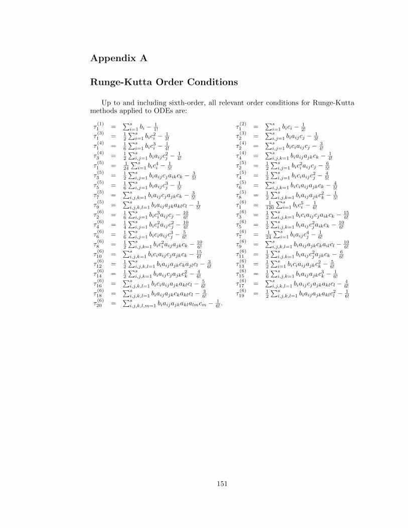
Appendix A
Runge-Kutta Order Conditions
Up to and including sixth-order, all relevant order conditions for Runge-Kuttamethods applied to ODEs are:
τ(1)1 =
∑si=1 bi −
11! τ
(2)1 =
∑si=1 bici −
12!
τ(3)1 = 1
2
∑si=1 bic
2i − 1
3! τ(3)2 =
∑si,j=1 biaijcj −
13!
τ(4)1 = 1
6
∑si=1 bic
3i − 1
4! τ(4)2 =
∑si,j=1 biciaijcj −
34!
τ(4)3 = 1
2
∑si,j=1 biaijc
2j − 1
4! τ(4)4 =
∑si,j,k=1 biaijajkck −
14!
τ(5)1 = 1
24
∑si=1 bic
4i − 1
5! τ(5)2 = 1
2
∑si,j=1 bic
2i aijcj − 6
5!
τ(5)3 = 1
2
∑si,j=1 biaijcjaikck −
35! τ
(5)4 = 1
2
∑si,j=1 biciaijc
2j − 4
5!
τ(5)5 = 1
6
∑si,j=1 biaijc
3j − 1
5! τ(5)6 =
∑si,j,k=1 biciaijajkck −
45!
τ(5)7 =
∑si,j,k=1 biaijcjajkck −
35! τ
(5)8 = 1
2
∑si,j,k=1 biaijajkc
2k − 1
5!
τ(5)9 =
∑si,j,k,l=1 biaijajkaklcl −
15! τ
(6)1 = 1
120
∑si=1 bic
5i − 1
6!
τ(6)2 = 1
6
∑si,j=1 bic
3i aijcj − 10
6! τ(6)3 = 1
2
∑si,j,k=1 biciaijcjaikck −
156!
τ(6)4 = 1
4
∑si,j=1 bic
2i aijc
2j − 10
6! τ(6)5 = 1
2
∑si,j,k=1 biaijc
2jaikck − 10
6!
τ(6)6 = 1
6
∑si,j=1 biciaijc
3j − 5
6! τ(6)7 = 1
24
∑si=1 biaijc
4j − 1
6!
τ(6)8 = 1
2
∑si,j,k=1 bic
2i aijajkck − 10
6! τ(6)9 =
∑si,j,k,l=1 biaijajkckailcl −
106!
τ(6)10 =
∑si,j,k=1 biciaijcjajkck −
156! τ
(6)11 = 1
2
∑si,j,k=1 biaijc
2jajkck − 6
6!
τ(6)12 = 1
2
∑si,j,k,l=1 biaijajkckajlcl −
36! τ
(6)13 = 1
2
∑si=1 biciaijajkc
2k − 5
6!
τ(6)14 = 1
2
∑si,j,k=1 biaijcjajkc
2k − 4
6! τ(6)15 = 1
6
∑si,j,k=1 biaijajkc
3k − 1
6!
τ(6)16 =
∑si,j,k,l=1 biciaijajkaklcl −
56! τ
(6)17 =
∑si,j,k,l=1 biaijcjajkaklcl −
46!
τ(6)18 =
∑si,j,k,l=1 biaijajkckaklcl −
36! τ
(6)19 = 1
2
∑si,j,k,l=1 biaijajkaklc
2l − 1
6!
τ(6)20 =
∑si,j,k,l,m=1 biaijajkaklalmcm −
16! .
151
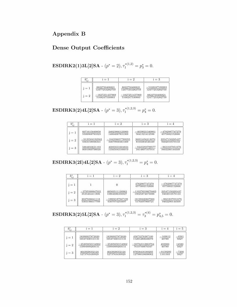
Appendix B
Dense Output Coefficients
ESDIRK2(1)3L[2]SA - (p∗ = 2), τ∗(1,2)1 = p∗3 = 0.
b∗ij i = 1 i = 2 i = 3
j = 1 882275040682112477253282759
882275040682112477253282759
−516824753088312477253282759
j = 2 −18272514379695168247530883
−18272514379695168247530883
882275040682112477253282759
ESDIRK3(2)4L[2]SA - (p∗ = 3), τ∗(1,2,3)1 = p∗4 = 0.
b∗ij i = 1 i = 2 i = 3 i = 4
j = 1 60716158498585506968783323
2482386612306014064067831369
−46390213408615641321412596
−47829877472794575882152666
j = 2 −91355041925625563158936341
−18435865778935534679930461469
369516562130708103384546449
225471502954379402010570133
j = 3 58848506211938091909798020
4009353160482413565043189019
−94452937995773414897167914
−86218370516769402290144509
ESDIRK3(2I)4L[2]SA - (p∗ = 3), τ∗(1,2,3)1 = p∗4 = 0.
b∗ij i = 1 i = 2 i = 3 i = 4
j = 1 1 0 47829877472794575882152666
−47829877472794575882152666
j = 2 −37955688470213535464411806
4858351113096310864686356927
−11027853867646319025874673088
225471502954379402010570133
j = 3 20278366411185303196617709
−188021879471996307074255697
181992208079005176497900721
−86218370516769402290144509
ESDIRK3(2)5L[2]SA - (p∗ = 3), τ∗(1,2,3)1 = τ
∗(4)3 = p∗4,5 = 0.
b∗ij i = 1 i = 2 i = 3 i = 4 i = 5
j = 1 1839093787202016547330141131
1839093787202016547330141131
4587327638710011281280648079
−16981240789
−65615827
j = 2 −2520565015496213994999269151
−2520565015496213994999269151
−837845128637647610748870347
49390040789
145805827
j = 3 46439283521245273763430929
46439283521245273763430929
8785841818920512798018608062
−81392001101303
−72005827
152
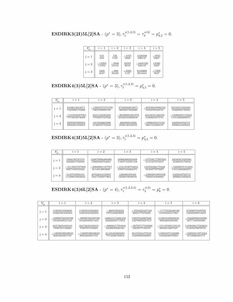
ESDIRK3(2I)5L[2]SA - (p∗ = 3), τ∗(1,2,3)1 = τ
∗(4)3 = p∗4,5 = 0.
b∗ij i = 1 i = 2 i = 3 i = 4 i = 5
j = 1 545644
7201127
−44554508
1528308938147
−65615827
j = 2 −1220511592
−304010143
323559016
−4445100938147
145805827
j = 3 18254347
−40030429
−23251127
81392002814441
−72005827
ESDIRK4(3)5L[2]SA - (p∗ = 3), τ∗(1,2,3)1 = p∗4,5 = 0.
b∗ij i = 1 i = 2 i = 3 i = 4 i = 5
j = 1 24486120549717422989170266
−130645272747697807639895795
472309028180719856057303060
−602306450863327645076548727
245459155952814520659176942
j = 2 −51435293070617773953874698
65531225832637765607547020
−8658088439187625322350989535
334185212363394189665475741
−5220683515322311015268282971
j = 3 39055678009549892491358055
14150228632865136633758329
4282560129562506140349505
−68084034151943867318289197
54228187627155898621095633
ESDIRK4(3I)5L[2]SA - (p∗ = 3), τ∗(1,2,3)1 = p∗4,5 = 0.
b∗ij i = 1 i = 2 i = 3 i = 4 i = 5
j = 1 10941267473746302601702029
12267909849049619860238704061
5096698692350611897153581109
−1375581779970059131337973237
245459155952814520659176942
j = 2 −31136537678098367169333422
−296889011679574114912804820
−3161453074484110807162464371
1455943861704289545977979287
−5220683515322311015268282971
j = 3 314570396219111339919304645
4076263415395319417583977863
1286985591691830973959079
−248628160034367385818498993
54228187627155898621095633
ESDIRK4(3)6L[2]SA - (p∗ = 4), τ∗(1,2,3,4)1 = τ
∗(4)3 = p∗6 = 0.
b∗ij i = 1 i = 2 i = 3 i = 4 i = 5 i = 6
j = 1 1196391038466512483345430363
1196391038466512483345430363
−286032646241970169629981
−35244254471832683177070205
−1717352244018610195024317061
2730887916970913030500014233
j = 2 −6999676033078818526599551455
−6999676033078818526599551455
10261017190510326266659717953
7495762390762012279805097313
1138531992356339983266320290
−842293925439506077740599399
j = 3 324736354294197030701510665
324736354294197030701510665
−388663172538416249835826165
−267057172238864265677133337
−1211053821431556658412667527
110202854750382451424476870755
j = 4 −146685286386238083464301755
−146685286386238083464301755
211034558850917774428730952
3015559147553315293695940061
11985337510208814336240079991
−636022139732246753880425717
153
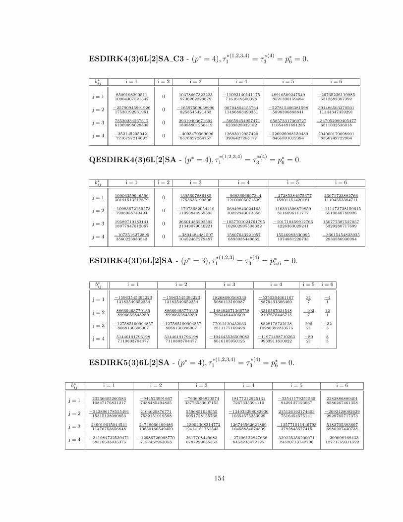
ESDIRK4(3)6L[2]SA C3 - (p∗ = 4), τ∗(1,2,3,4)1 = τ
∗(4)3 = p∗6 = 0.
b∗ij i = 1 i = 2 i = 3 i = 4 i = 5 i = 6
j = 1 850919829051110904307521542
0 103786673222239736262223679
−110931401411757161619500328
489165092475498521390159484
−267652361199855312882387392
j = 2 −2579094599192617530192931961
0 −165975090389908258545421433
9070480415576411486863490351
−2278154063815985898396888841
39148650337050111444347459291
j = 3 7353023426761761969698028838
0 2931940367169218088801260419
−566594549574716239828032182
65857331736072711054491681285
−3470529994054776511032536018
j = 4 −25214520504217216797214697
0 −40934703690968576827264757
126930129574203906427265177
−2269269881394398465891012384
2040001790989018366749722904
QESDIRK4(3)6L[2]SA - (p∗ = 4), τ∗(1,2,3,4)1 = τ
∗(4)3 = p∗6 = 0.
b∗ij i = 1 i = 2 i = 3 i = 4 i = 5 i = 6
j = 1 1990635994659630191513212679
0 13956978861851753633199896
−968369669734412100605071339
−2728538497537715901151420181
2307172388276611194553384711
j = 2 −100836721592737908958740494
0 −1707368205441911093844969395
5694984302416310222943013356
1163913068798598116096111777
−1114737381596456519848780926
j = 3 1958971018314118977847812067
0 2660148529259221349079040221
−1057701024761795162602995508332
−1017104599127664226363029241
1507773875270575329280717699
j = 4 −10735162728953560223983543
0 −380448448150710452467279487
158076432210576893035449662
155469823300951374881226733
−366154548230352830586936984
ESDIRK4(3I)6L[2]SA - (p∗ = 3), τ∗(1,2,3)1 = τ
∗(4)3 = p∗5,6 = 0.
b∗ij i = 1 i = 2 i = 3 i = 4 i = 5 i = 6
j = 1 −1596354539422313182549652254
−1596354539422313182549652254
182686905683305080413169087
−53503646611678879431386469
317
−41
j = 2 886694637701398996652843250
886694637701398996652843250
−1484920713667587963484430509
33105670245482197678446715
−1027
121
j = 3 −1275851909948578068130396907
−1275851909948578068130396907
770121204320332811177169428
882817873212810988392233575
29621
−323
j = 4 514461917961987110803704477
514461917961987110803704477
−1044435365090828616105950125
−119714987102639933911810022
−8021
83
ESDIRK5(3)6L[2]SA - (p∗ = 4), τ∗(1,2,3,4)1 = τ
∗(4)3 = p∗6 = 0.
b∗ij i = 1 i = 2 i = 3 i = 4 i = 5 i = 6
j = 1 2323660526058310847176831217
−9445239916677488485494825
−763605682057433776533607155
181772129251317267335394110
−335411792515359429127123667
22838868894018586267461358
j = 2 −24289617855549115315128090853
21046208767717532151019598
55968510495559051728155768
−13403329808293010354575253929
2151261921746037516454575141
−20924280026292929765717373
j = 3 24901961504454111476753656848
2474896649948610830160549459
−1300436831477212414161751345
12674656262186910458834074509
−1357710114467933792843577415
51837053836976980207430738
j = 4 −34198472253947138516533435375
−129867260987707127462963053
36177084496836787229655553
−274061228476668453233472125
32922535620007124520713742706
−20909816843312771759311522
154
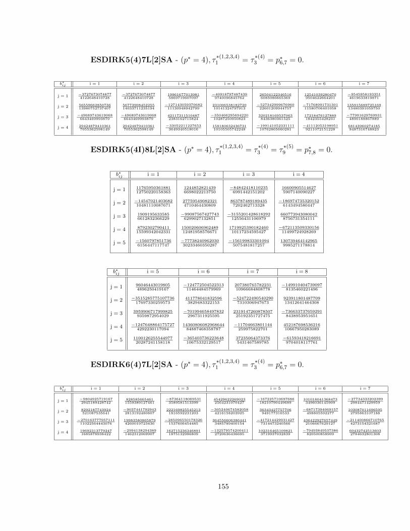
ESDIRK5(4)7L[2]SA - (p∗ = 4), τ∗(1,2,3,4)1 = τ
∗(4)3 = p∗6,7 = 0.
b∗ij i = 1 i = 2 i = 3 i = 4 i = 5 i = 6 i = 7
j = 1 −37276730748774122648410728
−37276730748774122648410728
199616770139815869719607097
−409187974874399740096845762
265041223465166085086665369
125410392804709504622664201
−95459581933514619633819871
j = 2 5655966285073613980752737407
5677390845225514033711235194
−12714305937068211130948942799
23100653818272010141324797913
−52734299967696022601209944757
−7176899173130111580706401058
13591568972516913480391059750
j = 3 −496897436190686643469993879
−496897436190686643469993879
421173115104872383162715824
−35046629569422010287250950823
3202181695370638436380361525
172184761278891842355428231
−779916297699314890188867889
j = 4 294248794103617055362598149
294248794103617055362598149
−330522112276533649340518016
15818063243673110105505742248
−19914105233111110762865660281
−411120531989519211072151228
681439602741858487316748823
ESDIRK5(4I)8L[2]SA - (p∗ = 4), τ∗(1,2,3,4)1 = τ
∗(4)3 = τ
∗(5)9 = p∗7,8 = 0.
b∗ij i = 1 i = 2 i = 3 i = 4
j = 1 1176595036188112750220158363
12448528214396698022213750
−848424181102356991442151202
166009055146275907140090227
j = 2 −1454702140368210481110087671
277595490823214710464430809
8637874891894357202462713328
−1869747353201526143494580447
j = 3 19091956335856612832366229
−990875674277436299027132851
−315520142861829212556431106979
6607739430800428756731354111
j = 4 879230279041115599342042331
15002060696248912481958576671
171992539018246010117234595427
−67211350933015611499724928269
j = 5 −15607978517366156447117747
−7773824096203030233460350287
−1561998333010945075481817257
1307394641429659985271178814
b∗ij i = 5 i = 6 i = 7 i = 8
j = 1 960464430198054896250419167
−12477250452231311464484579969
20738076578223110966684808778
−1499104047390978135460221496
j = 2 −351528577510773617697330259573
4117780418325963829483322153
−5247224905402907310306947673
92391180148770913412641464308
j = 3 39599067179998259359872954029
−7019946584978322967311925595
231914726087850725192351727475
−7366337376592918438953951651
j = 4 −12476488641757274292230117094
1436080608296864484887468358787
−11704663801144259975822701
45218769853621610667950283089
j = 5 110012625554497720287241158118
−36540373622364810675332129517
372350643733765431467589785
−615934182166919704018117761
ESDIRK6(4)7L[2]SA - (p∗ = 4), τ∗(1,2,3,4)1 = τ
∗(4)3 = p∗6,7 = 0.
b∗ij i = 1 i = 2 i = 3 i = 4 i = 5 i = 6 i = 7
j = 1 −98049257191672945189428742
8285856654611559389127461
−873641180695313589581513399
454296222690232564231070427
−16722571069768618210790449689
1010180413684733496036145909
−277343332023992984471429959
j = 2 8292187743924521087535641
−90374417929432813192480807
2221698255452131816592231203
−3052406745820584216158203925
36343427757706949177316533
−68717394069157498805592277
1030870116965952795863107188
j = 3 −27016377795711111022564443076
199835808658794260019723436
−2850965501783261537606454485
3645566063864413485789400154
−4172144299314277314473240566
4364229276574492106667629127
−2114008667107654273154321687
j = 4 196923137792471685878938422
−29941382943891462312069907
1627152363468911875132986809
−1325795742004112720636436695
1023164651098213719937032839
−79493849537386820500858909
604327425136032784632801308
155
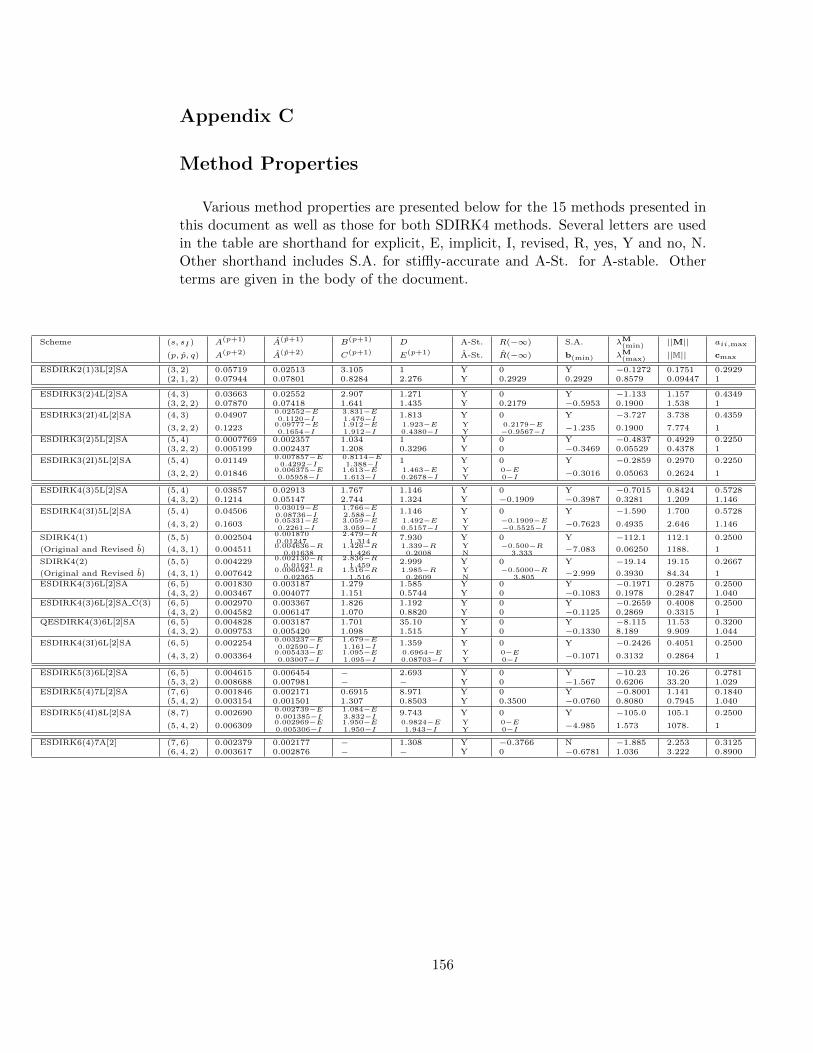
Appendix C
Method Properties
Various method properties are presented below for the 15 methods presented inthis document as well as those for both SDIRK4 methods. Several letters are usedin the table are shorthand for explicit, E, implicit, I, revised, R, yes, Y and no, N.Other shorthand includes S.A. for stiffly-accurate and A-St. for A-stable. Otherterms are given in the body of the document.
Scheme (s, sI ) A(p+1) A(p+1) B(p+1) D A-St. R(−∞) S.A. λM(min) ||M|| aii,max
(p, p, q) A(p+2) A(p+2) C(p+1) E(p+1) A-St. R(−∞) b(min) λM(max) ||M|| cmax
ESDIRK2(1)3L[2]SA (3, 2) 0.05719 0.02513 3.105 1 Y 0 Y −0.1272 0.1751 0.2929(2, 1, 2) 0.07944 0.07801 0.8284 2.276 Y 0.2929 0.2929 0.8579 0.09447 1
ESDIRK3(2)4L[2]SA (4, 3) 0.03663 0.02552 2.907 1.271 Y 0 Y −1.133 1.157 0.4349(3, 2, 2) 0.07870 0.07418 1.641 1.435 Y 0.2179 −0.5953 0.1900 1.538 1
ESDIRK3(2I)4L[2]SA (4, 3) 0.04907 0.02552−E0.1120−I
3.831−E1.476−I
1.813 Y 0 Y −3.727 3.738 0.4359
(3, 2, 2) 0.1223 0.09777−E0.1654−I
1.912−E1.912−I
1.923−E0.4380−I
YY
0.2179−E−0.9567−I
−1.235 0.1900 7.774 1
ESDIRK3(2)5L[2]SA (5, 4) 0.0007769 0.002357 1.034 1 Y 0 Y −0.4837 0.4929 0.2250(3, 2, 2) 0.005199 0.002437 1.208 0.3296 Y 0 −0.3469 0.05529 0.4378 1
ESDIRK3(2I)5L[2]SA (5, 4) 0.01149 0.007857−E0.4292−I
0.8114−E1.388−I
1 Y 0 Y −0.2859 0.2970 0.2250
(3, 2, 2) 0.01846 0.006375−E0.05958−I
1.613−E1.613−I
1.463−E0.2678−I
YY
0−E0−I
−0.3016 0.05063 0.2624 1
ESDIRK4(3)5L[2]SA (5, 4) 0.03857 0.02913 1.767 1.146 Y 0 Y −0.7015 0.8424 0.5728(4, 3, 2) 0.1214 0.05147 2.744 1.324 Y −0.1909 −0.3987 0.3281 1.209 1.146
ESDIRK4(3I)5L[2]SA (5, 4) 0.04506 0.03019−E0.08736−I
1.766−E2.588−I
1.146 Y 0 Y −1.590 1.700 0.5728
(4, 3, 2) 0.1603 0.05331−E0.2261−I
3.059−E3.059−I
1.492−E0.5157−I
YY
−0.1909−E−0.5525−I
−0.7623 0.4935 2.646 1.146
SDIRK4(1) (5, 5) 0.002504 0.0018700.01247
2.479−R1.314
7.930 Y 0 Y −112.1 112.1 0.2500
(Original and Revised b) (4, 3, 1) 0.004511 0.004636−R0.01638
1.426−R1.426
1.339−R0.2008
YN
−0.500−R3.333
−7.083 0.06250 1188. 1
SDIRK4(2) (5, 5) 0.004229 0.002130−R0.01621
2.836−R1.459
2.999 Y 0 Y −19.14 19.15 0.2667
(Original and Revised b) (4, 3, 1) 0.007642 0.006042−R0.02365
1.516−R1.516
1.985−R0.2609
YN
−0.5000−R3.805
−2.999 0.3930 84.34 1
ESDIRK4(3)6L[2]SA (6, 5) 0.001830 0.003187 1.279 1.585 Y 0 Y −0.1971 0.2875 0.2500(4, 3, 2) 0.003467 0.004077 1.151 0.5744 Y 0 −0.1083 0.1978 0.2847 1.040
ESDIRK4(3)6L[2]SA C(3) (6, 5) 0.002970 0.003367 1.826 1.192 Y 0 Y −0.2659 0.4008 0.2500(4, 3, 2) 0.004582 0.006147 1.070 0.8820 Y 0 −0.1125 0.2869 0.3315 1
QESDIRK4(3)6L[2]SA (6, 5) 0.004828 0.003187 1.701 35.10 Y 0 Y −8.115 11.53 0.3200(4, 3, 2) 0.009753 0.005420 1.098 1.515 Y 0 −0.1330 8.189 9.909 1.044
ESDIRK4(3I)6L[2]SA (6, 5) 0.002254 0.003237−E0.02590−I
1.679−E1.161−I
1.359 Y 0 Y −0.2426 0.4051 0.2500
(4, 3, 2) 0.003364 0.005433−E0.03007−I
1.095−E1.095−I
0.6964−E0.08703−I
YY
0−E0−I
−0.1071 0.3132 0.2864 1
ESDIRK5(3)6L[2]SA (6, 5) 0.004615 0.006454 − 2.693 Y 0 Y −10.23 10.26 0.2781(5, 3, 2) 0.008688 0.007981 − − Y 0 −1.567 0.6206 33.20 1.029
ESDIRK5(4)7L[2]SA (7, 6) 0.001846 0.002171 0.6915 8.971 Y 0 Y −0.8001 1.141 0.1840(5, 4, 2) 0.003154 0.001501 1.307 0.8503 Y 0.3500 −0.0760 0.8080 0.7945 1.040
ESDIRK5(4I)8L[2]SA (8, 7) 0.002690 0.002739−E0.001385−I
1.084−E3.832−I
9.743 Y 0 Y −105.0 105.1 0.2500
(5, 4, 2) 0.006309 0.002969−E0.005306−I
1.950−E1.950−I
0.9824−E1.943−I
YY
0−E0−I
−4.985 1.573 1078. 1
ESDIRK6(4)7A[2] (7, 6) 0.002379 0.002177 − 1.308 Y −0.3766 N −1.885 2.253 0.3125(6, 4, 2) 0.003617 0.002876 − − Y 0 −0.6781 1.036 3.222 0.8900
156


REPORT DOCUMENTATION PAGE Form ApprovedOMB No. 0704–0188
The public reporting burden for this collection of information is estimated to average 1 hour per response, including the time for reviewing instructions, searching existing data sources,gathering and maintaining the data needed, and completing and reviewing the collection of information. Send comments regarding this burden estimate or any other aspect of this collectionof information, including suggestions for reducing this burden, to Department of Defense, Washington Headquarters Services, Directorate for Information Operations and Reports(0704-0188), 1215 Jefferson Davis Highway, Suite 1204, Arlington, VA 22202-4302. Respondents should be aware that notwithstanding any other provision of law, no person shall besubject to any penalty for failing to comply with a collection of information if it does not display a currently valid OMB control number.PLEASE DO NOT RETURN YOUR FORM TO THE ABOVE ADDRESS.
Standard Form 298 (Rev. 8/98)Prescribed by ANSI Std. Z39.18
1. REPORT DATE (DD-MM-YYYY)01-03-2016
2. REPORT TYPE
Technical Memorandum3. DATES COVERED (From - To)
01/2011-03/20164. TITLE AND SUBTITLE
Diagonally Implicit Runge-Kutta Methods for Ordinary DifferentialEquations. A Review
5a. CONTRACT NUMBER
5b. GRANT NUMBER
5c. PROGRAM ELEMENT NUMBER
5d. PROJECT NUMBER
5e. TASK NUMBER
5f. WORK UNIT NUMBER794072.02.07.02.03
6. AUTHOR(S)
Kennedy, Christopher A., and Carpenter, Mark H.
7. PERFORMING ORGANIZATION NAME(S) AND ADDRESS(ES)
NASA Langley Research CenterHampton, Virginia 23681-2199
8. PERFORMING ORGANIZATIONREPORT NUMBER
L–20597
9. SPONSORING/MONITORING AGENCY NAME(S) AND ADDRESS(ES)
National Aeronautics and Space AdministrationWashington, DC 20546-0001
10. SPONSOR/MONITOR’S ACRONYM(S)NASA
11. SPONSOR/MONITOR’S REPORTNUMBER(S)
NASA-TM–2016–219173
12. DISTRIBUTION/AVAILABILITY STATEMENT
Subject Category 02Availability: NASA STI Program (757) 864-9658
13. SUPPLEMENTARY NOTES
14. ABSTRACT
A review of diagonally implicit Runge-Kutta (DIRK) methods applied to first-order ordinary differential equations (ODEs) isundertaken. The goal of this review is to summarize the characteristics, assess the potential, and then design several nearlyoptimal, general purpose, DIRK-type methods. Over 20 important aspects of DIRK-type methods are reviewed. A designstudy is then conducted on DIRK-type methods having from two to seven implicit stages. From this, 15 schemes are selectedfor general purpose application. Testing of the 15 chosen methods is done on three singular perturbation problems. Based onthe review of method characteristics, these methods focus on having a stage order of two, stiff accuracy, L-stability, highquality embedded and dense-output methods, small magnitudes of the algebraic stability matrix eigenvalues, small values ofaii, and small or vanishing values of the internal stability function for large eigenvalues of the Jacobian. Among the 15 newmethods, ESDIRK4(3)6L[2]SA is recommended as a good default method for solving stiff problems at moderate errortolerances.
15. SUBJECT TERMSnumerical methods,ordinary differential equations, Runge-Kutta,diagonally implicit,L-stability,dense output,stage-valuepredictors,discontinuities
16. SECURITY CLASSIFICATION OF:
a. REPORT
U
b. ABSTRACT
U
c. THIS PAGE
U
17. LIMITATION OFABSTRACT
UU
18. NUMBEROFPAGES
162
19a. NAME OF RESPONSIBLE PERSON
STI Help Desk (email: [email protected])
19b. TELEPHONE NUMBER (Include area code)
(757) 864-9658