Computational Mechanics 16 (1995) 426-436 �9 Sprmger-Verlag 1995

Development of new spatially curved frame finite element for crash analysis Part 1" Formulation and validation

S. Vasudevan, H. Okada, S. N. Atluri

426 Abstract This paper deals with the development of a new space curved frame finite element to be used for crash analysis (non-linear). The formulation has been validated for problems of large deflection and rotation, and for problems involving initially curved members. Based on the validation performed, it is expected that crash problems may be modeled using a single element per member thus retaining computational efficiency while performing an accurate analysis.

1 Introduction This research seeks to develop a computational methodology which can be used to improve the existing crashworthiness analysis codes for aircraft structures. The computational methodology will be tested through a research code and may be implemented in KRASH to provide it with the following additional features (KRASH-2000).

(1) Detailed spatial frame analysis (including large deflections, rotations and structural collapse-failure). (2) Overall analysis of aircraft crash with large deflections and rotations and incorporating structural collapse. (1) is discussed in this paper, and (2) shall be discussed in future publications.

1.1 Overview of technical approach 1) The kinematics for a beam undergoing large deflections with

transverse shear deformation being accounted for, as developed by Iura and Atluri (1989), is used in the derivation of the frame element.

2) The functional for a beam in terms of the stress and moment resultants, displacement of the beam axis and rotation of the beam section, stretch and the curvature of the beam is derived (4 geometric and 2 stress like terms). The stationary condition of this functional enforces compatibility conditions, linear and angular momentum balance laws and the constitutive relation in their weak forms.

Communicated by S. N. Atluri, 30 June 1995

S. Vasudevan, H. Okada, S. N. Atluri Computational Modeling Center, Georgia Institute of Technology, Atlanta, 6A 30332, USA

Correspondence to: S. N. Atluri

The support of this work by the FAA, under a grant to the Center of Excellence for Computational Modeling, is gratefully acknowledged.

3) The stretch and curvature are eliminated using the strong form of the constitutive relation (written in terms of the stress and moment resultants).

4) The problem is hence reduced, with two geometric variables (displacement and rotation) and the stress and moment resultants.

5) Hence, the independent variables in the problem are the rotation of the cross-section, the deflection of the center line of the beam section, and the stress and moment resultants. The linear and angular momentum balance taws as well as compatibility conditions are enforced in the weak forms, over the span.

6) Structural collapse is accounted for using the hinge formulation.

The formulation of a space frame element (structural hinge formation included) to be used in the detailed space frame analysis (under crash loading) has been completed and is discussed in this paper. The new element was validated for geometrically non-i/near problems and problems involving initially curved members using just one element per member. Hence, it is seen that the element is computationally quite effective. The new element will be implemented in a research code to study typical impact problems. The frame structures will be modelled with just one element per member with this formulation.

2 Kinematics, constitutive relation and variational principle for an initially curved member of a space-frame

2.1 Geometry of the undeformed and deformed frame For the sake of clarity and completeness, the kinematical relations of the curved member, developed by Iura and Atluri (1989), are summarized below.

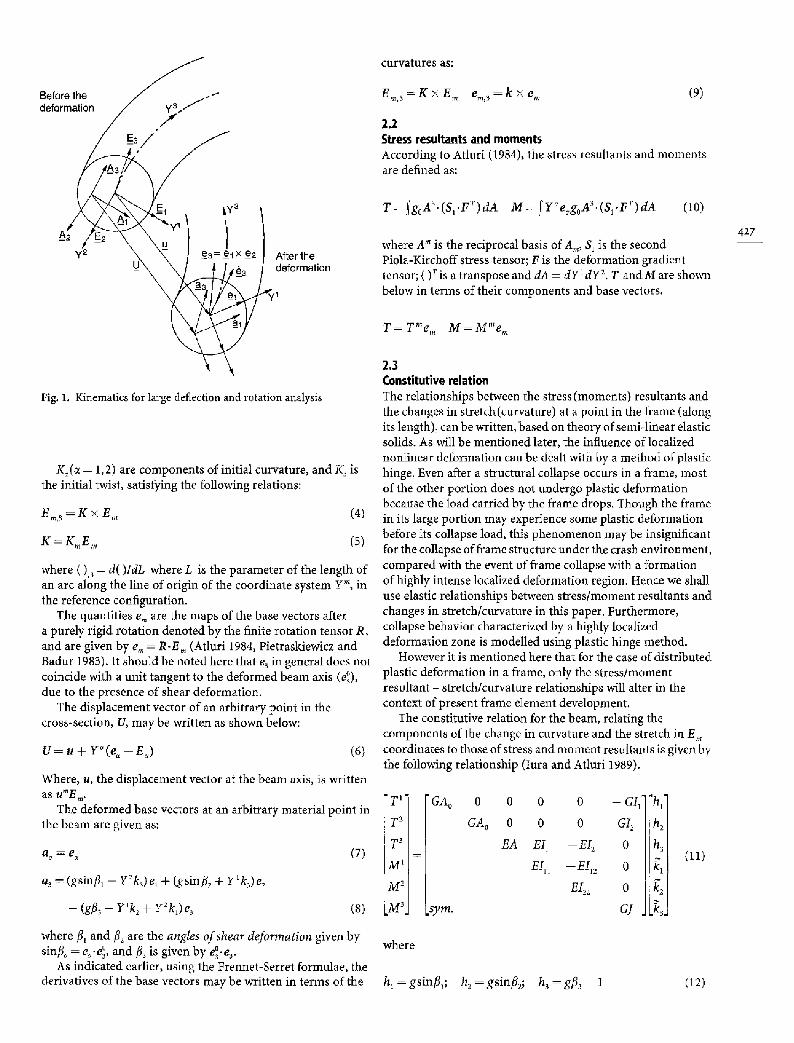
Let Y m (m = 1, 2, 3) be a convected orthogonal curvilinear coordinate system. The coordinates Y= (~ = 1, 2) are taken in the cross-section, while the coordinate y3 is taken along the beam axis, as shown in Fig. 1. The undeformed base vectors at an arbitrary point in a cross-section, is expressed in terms of the undeformed unit base vectors E~ at the beam axis, as shown below:

G=E~ (1)

A 3 = - - y2K3E ~ + Y~K3E 2 +goE3 (2)

where

go = 1 -- Y 1 K 2 + Y Z K 1 (3)

Before the deformation / ,

curvatures as:

E,~,3 = K x E m era, 3 = k x e m (9)

2.2 Stress resultants and moments According to Atluri (1984), the stress resultants and moments are defined as:

y2 U ~ ~ ~a= ~1• e2 After the i / .,~_ deformation

T = S g o A 3 . ( S , . F T ) d A M = S Y ~ e ~ g o A ~ . ( S 1 . F r ) d A (10)

where A m is the reciprocal basis of A m, S 1 is the second Piola-Kirchoff stress tensor; F is the deformation gradient tensor; ( )ris a transpose and dA = d Y ~ d Y 2. T andM are shown below in terms of their components and base vectors.

T = Tm em M = M m em

427

Fig. l. Kinematics for large deflection and rotation analysis

K s (~. = 1,2) are components of initial curvature, and/(3 is the initial twist, satisfying the following relations:

Em, 3 = K • E m

K = K m E m

where ( ),3 = d( ) ldL where L is the parameter of the length of an arc along the line of origin of the coordinate system Y~, in the reference configuration.

The quantities e m are the maps of the base vectors after a purely rigid rotation denoted by the finite rotation tensor R, and are given by e~ = R ' E m (Atluri 1984, Pietraskiewicz and Badur 1983). It should be noted here that e 3 in general does not coincide with a unit tangent to the deformed beam axis (e~), due to the presence of shear deformation.

The displacement vector of an arbitrary point in the cross-section, U, may be written as shown below:

U = u + Y ' ( e ~ - - E ~ )

2.3 Constitutive relation The relationships between the stress (moments) resultants and the changes in stretch (curvature) at a point in the frame (along its length), can be written, based on theory of semi-linear elastic solids. As will be mentioned later, the influence of localized nonlinear deformation can be dealt with by a method of plastic hinge. Even after a structural collapse occurs in a frame, most of the other portion does not undergo plastic deformation because the load carried by the frame drops. Though the frame

(4) in its large portion may experience some plastic deformation before its collapse load, this phenomenon may be insignificant (5) for the collapse of frame structure under the crash environment, compared with the event of frame collapse with a formation of highly intense localized deformation region. Hence we shall use elastic relationships between stress/moment resultants and changes in stretch/curvature in this paper. Furthermore, collapse behavior characterized by a highly localized deformation zone is modelled using plastic hinge method.

However it is mentioned here that for the case of distributed plastic deformation in a frame, only the stress/moment resultant - stretch/curvature relationships will alter in the context of present frame element development.

The constitutive relation for the beam, relating the components of the change in curvature and the stretch in E m

(6) coordinates to those of stress and moment resultants is given by the following relationship (Iura and Atluri 1989).

Where, u, the displacement vector at the beam axis, is written as umErn.

The deformed base vectors at an arbitrary material point in the beam are given as:

a~ = e~ (7)

a3 = (gsinfll - Y2k3)e, + (gsinfi2 + Ylk3)e2

(8) + (g~3 - y lk2 + y2kl)e3

where fl, and fi2 are the angles o f shear d e f o r m a t i o n given by sinfl= = e=. e~ and fi3 is given by e~

As indicated earlier, using the Frennet-Serret formulae, the derivatives of the base vectors may be written in terms of the

�9 T 1,

T 2

T 3

M 1

M 2

m 3 '

GA o 0 0

GA o 0

E A

s y m .

0 0 - GI

o o cI~

EI~ -- E I 2 0

E I n --EI12 0

EI= 0

GI

'hi"

hi

h3 ~ ( 1 1 ) kl

k2

,k3=

where

h 1 = gsinfi,; h2 = gsinfi2; h3 = gfl3 - 1 (12)

428

k" is change in curvature

A = fgodA A o = k A I~= f r~godA

I12=fY1y2godA I22=~(YZ)ZgodA l = ~ p g o d A (13)

The factor k is a shear-correction factor (Cowper (1966)). It is important to note here that some of the inertia terms (such as I~2) vanish on choosing a suitable coordinate system.

The strain energy function I4~ (which may be derived from the above stress strain relationship) is expressed as:

W, = �89 2 + GAo(h2) 2 + EA(h3) 2 + EIII (k'~l) 2

+ EI22 (k2) 2 + GJ (k3) 2 + 2EI~h3k2 - 2EI2h3 J~ 2

- 2EI12kl k 2 - 2GI lh lk 3 + 2GI2h2kf] (14)

2.4 General mixed variational principle As first shown by Fraejis de Veubeke (1972) and later generalized by Atluri and Murakawa (1977), a general mixed principle, for a 3-dimensional elastic material, and involving the first Piola Kirchoff stress tensor tl, the right stretch tensor U, the finite rotation tensor R and the displacement vector v as variables, can be stated as the stationary condition of the functional F~:

Fl(tt, U,R,v) = ~ [W0 (V) + t[: ((I + Vo v ) r - -R - U) -- po[J �9 v]dV o

-- S t . vds - ~t. (v - 9)ds (15)

where W 0 is the strain energy function, P0 the mass density in the undeformed state, b-the body force vector per unit mass, l the traction on the boundary per unit undeformed area and V0 the gradient operator in the undeformed state. It should we noted that the rotation tensor R may be written in terms of a rotation vector as e '~• (Pietraskiewicz and Badur, 1983, and Atluri and Cazzani, 1995).

Using the kinematic and constitutive relations mentioned earlier, Iura and Atluri (1989) derived the functional for the beam, and on imposing the stationary condition obtained the below equation.

+ f T . ((x + u),3 - R. (h + E3)) + 3M. (/3 -- R .k)

-- (T,3 + q ) . f u -- (M,3 + (x + u) 3 • T ).3dp]dL

- so f r . ( u - a) + fM-(4,-- ~,) =0

-- [s fU.(gl-- T) + fdp.M ]~==~ = 0 (16)

Where 6~b and/3 are defined so as to satisfy 6~b x I = fir .R r and 13 x I = R,3. R r. (Following [Atluri 1984] and [Pietraskiewicz and Badur 1983] respectively).

3 Development of finite element formulation The reason we use the variational principle in Eq. (15) is that on imposing the stationary condition, the condition of balance of angular momentum is independent of the constitutive relation. It is also worth noting here that the curvature is defined as the derivative of the tangent vector with respect to the arc length parameter and hence it is not well behaved (note: the curvature may have steeper variations than the displacement and the curvature becomes singular on hinge formation).

One may obtain the changes in curvatures and stretch by differentiating the displacement or rotation field. It is however noted that such operations (leading to a displacement finite element) would not give a singular nature for curvatures. Furthermore, the variations would be one order lower from that of rotations and two orders lower than that of displacements. Thus many elements are needed to represent required deformation.

On the other hand, the variations of stress and moment resultants are determined by the current configuration of the frame. Especially, the stress resultants do not vary in the absence of body, inertia or any distributed forces. Therefore, it is far easier to assume the stress and moment field than deriving those from the kinetic variables. Also, it is quite simple to derive the changes in curvatures and stretches from the stress and moment resultants as done below.

Thus we use the strong form of the constitutive relation to eliminate the stretch and the curvature (in terms of the moment and stress resultants by inverting the constitutive equation) while imposing compatibility, linear and angular momentum balance conditions in their weak forms. Consequently the stationary condition was simplified as shown below.

fF1 = S [fiT. ((x + u).3 -- R. (h + E 3)) + fM. (l 3 - R. k)

- (T3 + q ) . f u - (M3 + (x + @3 • T) . f4~]dL

- - 4 ~ ) ] ~ : 0 [ s f T . ( u - f t ) + f M . ( d p - L=I

L = l _ - [ s f u . ( ~ - T) + f r ] ,=0- 0 (17)

On inverting the constitutive relation, the stretch and curvature may be written as

h----HT.T + H M . M

I t= K~. T + K~z.M, (18)

thus reducing the number of independent variables to four. Note H r, H M, K T and K M are (3 • 3) obtained by inverting the (6 • 6) matrix in Eq. (11).

3.1 Discretization procedure and derivation of tangent stiffness matrix

3.1.1 Overview of discretization procedure The below development is quite general and assumes linear trial functions for the three components of all the four variables (stress resultant, moment resultant, displacement and rotation) as indicated below. In the absence of distributed loading the procedure is simplified greatly as the stress resultant is a constant.

T ' = - T * , 7 + T 2 1 - - ' ' + M ' 2 1--

u' = u', ~ + u' 2 1 - - co--co, t +co2' 1--

3.1.2 Equations obtained from stationary condition a) Expression (19) is now substituted into Eq. (17). The integrated terms and boundary terms are evaluated giving us Eq. (20) in matrix form (keeping in mind the relation between the base vectors e, = R .E,) . b) We then invoke the condition that the variation in each of the components of the four variables at both the nodes are arbitrary and independent (b T~, c~ T2', cSM~, 5M2' , (~U'I, (~Ul2 , (~(J)'l' (~(~ giving us a system of Eq. (21).

Consequently 24 equations are obtained in 24 unknowns as shown in the subsequent discussions. Quite often, however, while dealing with 1D or 2D problems, problems with displacement specified boundary conditions, or problems without distributed loading, the number of components and equations involved reduces substantially. For instance, in the example presented, due to the absence of distributed loading, the stress resultant was assumed to be a constant, furthermore it was a planar problem, thus greatly simplifying the problem.

429

for i = 1,2,3 (19)

It is important to note here that T' and M' refer to the components in e, coordinates while u' and (# refer to the components in E, coordinates. The subscripts 1 and 2 indicate that the variable is defined at the nodes 1 and 2 of the frame element, respectively.

The behavior of to, u, T and M are illustrated below.

a) T (Stress Resultant): Constant trial functions give the exact solution for a problem where there is no distributed loading.

b) M (Moment Resultant): From the strong form of the angular momentum balance condition, it may be seen that the order of M is one more than the order of T when the displacements are small. Hence linear trial functions are suitable for the moment resultants.

c) r (Finite Rotation Vector): From the definition of r = e ~ x ~, Section 2.4) it can be seen that with a linear variation of to, we obtain a higher order variation of R.

d) u (Deflection of the Beam Axis): Quadratic trial functions may appear to be necessary based on the compatibility conditions even for small deformation problems (since r is assumed to vary linearly). However only linear functions are assumed for the displacement based on the example mentioned below.

Consider the example of a cantilever beam loaded at one end by a constant force normal to the axis and undergoing small deformations. It is well known that the variation of the deflection and the rotation are cubic and quadratic respectively. Using the formulation we have derived, treating the entire cantilever beam as one element, we obtained the exact and deflection using just linear functions for u, to, M and constant for T. It should be noted that in the formulation derived the rotation and the displacement are independent variables and so are the stress and moment resultants, thus we have a mixed formulation where lower order elements are quite effective and locking is less likely.

�9 . . m bT,11 or

bT, 21 ocotl

~T? I Ocofi [B~(lx3) Bmx3)] 6T) I +[A•,• A2(lx3)] 0coil

6T21 0~o~i

+ [ c t + . G . + Ea,~)] E~ox3 ) *

+ [ D ~ + * El(1 x 3)

~co', ~co~ ~co~

&4 aco]

,~ (/)~, 6 X l

, 6 M ) I

g~MY l

6M,31 D2 +F2<~x3)] 6 M ) I

* distr, load] q- [G~(, x 3) G2(1 • 3)

~M?I

.aMZJ x,

�9 , ~u ~, au, ~

au 3,

au~

au~

.&~. ~ •

430

+ [ c 7 + * E~(~ x 3)

, ,

6~oI 6co~

cs~ C ; 'q-- E~( 1 x3)] ! 6(,0~

,6co~, ~x~

+ [q~+ TR'~(~• q'~ + T R ~ •

�9 m

O u : I

OuT I

Ou~ I

ou~ I

ou~ I

.o u q 6 • 1 J 1

* MRS1 • + [MRm • 3)

O~O~l

OCO~l

0r I

o ~ I

O(D~J 6 x l

(20)

(The details of the matrices A~, B~, etc. are discussed later) Since the variations of

6T! l bM~ 6ut i oco: l

6T2,1 6M~ 6u~i 66o~,1

6T3,1 6M~ 6u~ 6co? l

6T~ I' 6M~ ' bu~ ' oco: l

6T~ l 6M~ 6u~ 6toni

1 are arbitrary and independent, on rearranging the corresponding coeffecients of 6T~, 3Mj, 6o~ and 6u~ in Eq. (19), the below system of equations are obtained.

* = [ 0 ] ( 1 • Bmx3)

* = [ 0 ] ~ • B2(x x 3)

D ~ + F~I x3) = [ 0 ] ( 1 x3)

D; + F~I • = [01(i •

A~ + C? + E~ + H~ + ]~ + MR'~(I• ~ = [ 0 1 ( l X 3 )

~r A* + C'~ + E~ + H? + J~ + MR m • = [01(1 •

G~f + TR'~ * = [ 0 ] . + q1(1 x 3) x 3)

G~ + TR'~ + q~l • [0](1 • (21)

The details of the above equations are discussed below and specific values for an example are given in section (3.3). The various terms in condition (17) that are referred to in the following discussion are also listed.

Term 1 ~ ~6T. ((x + u).3 - R . (h + E3)) dL Column vectors A~, A~ and B~, B~ in Eq. (20) are derived

from the first term of R.H.S. in Eq. (17). Since, we assume the variation of the components of stress resultants, additional terms (B~ and B~) arise from expression for 6T as shown below: bT = 6T'e, + T*6e, and 6e, = 6R .E,. Note: 6R is written in terms of boo through the relation 6R = (6~ • I).R (note: bq~ is written in terms of 6o), to and it's derivatives (Iura and Afluri 1989)).

Hence the first terms of R.H.S. in Eq. (17) give the first two terms in the L.H.S. of expression (20). It can be seen that the terms associated with &@ 6eY 2 and 6T1, bT~ correspond to the column vectors A~, A~ and B~*, B~ respectively. The nature of these column vectors are discussed below.

B~ and B f - B~ and B~ depend on the derivative of the displacement vector (depends on the initial curvature), the rotation tensor (which is written in terms of the rotation vector using the relation R = e ~• and the stretch (written in terms of the stress and moment resultants through the constitutive relation). Consequently it is a function of the components of all four variables and depends on the initial curvature and the material properties (Hr, HM) as well.

A~ and A~ - They multiply the variations in the components of the rotation vector at the two nodes. It can be seen that this term involves the components of the stress resultant, the derivatives of the displacement vector (depends on the initial curvature), the rotation and the stretch (written in terms of the stress and moment resultants through the constitutive relation). Consequently they are functions of the components of all four variables and depend on the inital curvature and the material properties (H r Hu) also.

T e r m 2 ~ M . ( / 3 -- R . k )dL The resulting discretized equations derived from this term has similar structure to those obtained from the first term in Eq. (20). As the case of the stress resultants, the variation of the moment resultants are expressed in terms of the change of the components and of the base vectors. Hence, they are shown to be: 6M = 6M~ei + M'6e A again 6e, = 6R .E v Note: 6R is written in terms of &o through the relation 6R = (64 • I).R.

Hence the column vectors associated with 60)~, &0~ and 6M'1, 6M~ correspond to the column vectors (C7 + ET), (C; + E;) and (D~ + F~), (D; + F;) respectively (Eq. (20)). Column vectors C~, C; and Dl% D; have arisen from terms involving 13. The other column vectors, namely E~, E ; and F~, F ; have arisen from the terms involving R-k.

C~ and C; arise from (M*6G) �9 l 3 (note: As explained earlier 6e i is written in terms of &o). They multiply the variations in the components of rotation. These are functions of the components of moment resultants and the rotation vector and depends on the initial curvature.

D~ and D; are derived from the term (6M'G).I r These column vectors are functions of the rotation vector and its derivatives.

E l and E~ are derived from the term (M'6el). (R. k). These column vectors are functions of the components of all independent variables except displacement, since the change in curvature k are written in terms of the stress and moment resultants through the matrices K r and K M (material property).

F~* and F~ are obtained from (3M'G). (R ./~). They are also functions of all independent variables except for displacement, and they depend on the material properties ( K r and KM).

Term 3 ~ ( ( T 3 + q).6u)dL Gl* and G[-Obtained from the third term in condition (17). It multiplies the variations in the components of displacement at the two nodes. This term depends on the components of all variables and also the material properties (K r and KM).

T e r m 4 ~ ( M 3 + (x + u),3 x T).bdpdL The fourth term in condition (17) may be split into two parts, M3.3q~ and ((x + u).3 x T).fqk

//1" and 1-12" are obtained from the first part. It multiplies the variations in the components of the rotation vector at the two nodes(note: 6~ is written in terms of 6to, r and it's derivatives (Iura and Atluri 1989)). This term depends on the components of the stress, moment resultants and the rotation vector. It also depends on the material properties (K r and KM).

J~* and ]2" are obtained from the second part of the fourth term in condition (17), namely ((x + u) 3 • T).bqk It multiplies the variations in the components of the rotation vector at the two nodes (note: 3q9 is written in terms of 3o~, co and it's derivatives (Iura and Atluri 1989)). It is seen that this term depends on the components of the displacement, rotation and the stress resultant as well as the initial curvature.

Boundary Term (Traction specified) -- [s bU'(fl-- T) + bdp.M ]L=l L = 0

ql* and q~; TRY{ and TRy; MR~ and MR; - The first two pairs are obtained from the first part of the traction boundary condition. It multiplies the variations in the components of the displacements. TR~ and TR2* is a function of the components of the stress resultant and the rotation vector (note: e i = R .E) while q~ and q2* correspond to the end load applied. MR~ and MR2 depend on the moment resultant and the rotation and it multiplies the variation in the components of the rotation. None of these terms depend on any geometry or material dependent parameters. The trial functions may be easily chosen to satisfy some of the boundary conditions in the strong form and this term may be simplified further.

3.2 Derivation of tangent stiffness matrix As shown in the earlier section 24 scalar equations (system of equations 21) are obtained in 24 unknowns (4 variables, 3 components, 2 unknowns). It can be seen that the equations are highly coupled. Hence, we use Taylor's expansion (used as a linearization procedure) to relate the incremental displacements explicitly to the applied loading as explained in the following discussion.

By using Taylor's expansion, the value of a function at a point (Xx, x~ ...... G) may be written in terms of the value at a point in it's neighbourhood (x~, x~ ...... x~ and the increments (Xl-X~, X2-X ~ . . . . . . Xn-xOn) as shown below:

f(Xl, X 2 .... Xn ) _ o 0 o -- X~) - - f (xvx2 .... G) + (Xl

\cx2/ \ o x , /

We now focus our attention to system of Eq. (21). The right hand sides of the equations are row matrices which we shall write in terms of their scalar components as indicated below:

B ~ [ B ~ B~2 B~]

B~-~ [B~ B~ B2~ l

DI* + F T ~ [D ~ D~ D~]

D2* + F ; ~ [D2~ D~2 D2~]

A~ + C 7 + E l + H i + 1~ + MR 1 ~ [All A,2 A,3 ]

A~ + C~ + E; + H ; + ]~ + MR2*~ [A~ A2~ Az~ ]

G~ + TRT + q ~ [ G ~ G~ G~31

It is worth emphasizing that the above row matrices are in general functions of the components of the nodal displacements, rotations, stress and moment resultants. It should also be noted that the G~'s are weighted functions of the applied load. Using Taylor's expansion, we now express the values of the scalar components (A~, B**j, D'andes G*v i = 1,2 j = 1,2,3) in terms of their values at an initial state and the corresponding increments in the components of the nodal displacements, rotations, stress and moment resultants. Consequently, the system of Eq. (21) is rewritten to relate the incremental values (of the nodal components of the displacements, rotations, stress and moment resultants) to the applied loading.

fA 12x12 atr B lZx12Matr l[ =I C(12 x 12Matrix) D(12 x 12Matrix)J A

(22)

431

432

The block matrices A,

OB~ OB~ OT~ OT 2

OB~ OB~ OT) OT~ z

OB~ OB~

~T~ ~T~

OB~ OB~

o~: OT? OB~ OB~ OT) OT t

OB~ OB~ OT) OT 3

A= OD~ OD~ OT) eT 2

OD~ OD~ or) OT~ OD~ OD~ O N OT(

~D~ OD~ OT) o~rt

OD~ 2 OD~ 3T) OT?

~D~ OD~ o~t OTt

similarly B, C, D (12 •

-aB~ &o' 1

B = . . . . . . . . . .

0D~

&O~l

- (~A ~1 aT, ~

C =

0G~ 0T)

"0At1 &o]

D = , ~ . . . . . . . .

,ga~ &o',

B, C, D and P, V, X are listed as follows.

OB~ OB~ OB~ OB~ OB~ OB~ OB~ OB~ OB~ OB~ OT~ OT~ OT~ OT~ OM) OM~ OM~ OM~ OM~ OM~

OB~ OB~ OB~ OB~ OB~ OB~ OB~ OB~ OB~ OB~ 0 T 3 0 T~ 0 T~ 0 T 3 OM~ OM 2 OM( OM~ OM 2 OM~

OB~ OB~ OB~ OB~ OB~ OB~ OB~ OB~ ~B~ OB~ 0 T( 0 Td 0 T: 0 T~ OM) OM? OM: OM~ OM 2 OM~

OB~ OB~ OB~ OB~ OB~ OB~ OB~ 3B~ OB~ OB~ 0 T~ 0 Td 0 Td 0 Td OM~ OM z OM~ OM~ OM~ OM~

OB~ OB~ OS~z OB~ OB~ OB~ OB~ OB~ OB~ OB~ 0 T~ 0 Td 0 rd 0 Td OM) OM~ OM~ OMd OM 2 OM~

OB~ OB~ OB~ OB~ OS~ OB~ OB~ OB~ OB~ OB~ 0 T 3 0 T~ 0 T22 0 T~ OU) c~M~ OM( ~M~ OM 2 OM~

OD~ OD~ OD~ ODF, OD~ aD~ OD~ OD~ OD~ OD~ OT? OT~ OT 2 OT~ OM( OM? OM~ OM~ OM~ OM~

OD~ ~D~ OD~ 2 ~D~ OD~ OD~ OD~ OD~ OD~ OD~ OT( OT~ ~r~ OT~ ~M) OM 2 OM~ ~M~ OM~ ~M~

OD~ OD~ OD~ OD~ OD~ OD~ aD~ OD~ OD,~ ~D~ 3T( OTd OT~ 3T~ OM) OM z OM~ OM~ OM~ OM~

OD~ OD~ OD~ OD~ ~D~ OD~ ~D~ OD~ OD~ OD~ OT~ OTd OT~ c~T~ OM) OM~ OM~ OM~ OM~ OM~

OD~ OD~ OD~ OD~ OD~ ~O~2 OD2~ OD~ OD~ OD~ OT( OTd OT~ OT~ OM t OM~ OM~ OMd 3M: OM:

OD~ OD~ OD~ OD~ OD~ ~D~ ~D~ OD~ OD~ ~D~ OT( 0 T~z O T 2 OT i OM~ OM~ OM~ OM~ OM 2 OM~

12) are given by

0u]

OD* 3 Ou] .

OA~, OM~

aa~3 0M32.

OA~I" aul

ac~ 0u]

(23)

'ATIi "

AT2~ AT~

AT~

AT~

A P = AT~ AM11

AM

AM: AM

AM~ AM~

A V =

�9 i

Ao)~ I A6o, ~ I A~o, ~ I

Atoll

A~O~l AoXI

Au~l Au,~l

Au, ~ I

Au~ I / xu~ l

.Au]~

X =

�9 i �9 m

B,*, I A ~ I

B ~ ] A ~ I

B ~ ] A ~ I

B$, ] A~ , I

B~*~ I A ~ I Y(q) =

D ~ I G,*,[

D;I G~l

D * G* �9 2 3 J . 2 3 J

We now condense the system of equations obtained to relate the incremental displacements to the applied load (note: block matrix Y is also represented as Y(q) to indicate that it is a weighted function of the end load and the distributed loading)

AAP + BA V = X CAP + DA V = Y We may condense this equation as shown.

AP=A-I(X--BAV) (D--CA 1B)AV=Y--CA-1X (24)

Renaming the variables D -- CA-~B = D* and Y - CA ~X = Y *

and partitioning D* into four block matrices (6 x 6 each), AV into two (6 x 1) matrices and Y* into two (6 x 1) matrices, Eq. (24) may be rewritten as:

IDa D TVA q__[-Y:(6 • 1) 1 D~ D~2JLAu* j _ Y ; ( 6 • 1)

(25)

Note: AV = [_Au* A LY:J

Acol Aul ao, ~ au~

aco*= aco~ au*-- au~ a~o~ au~ a~o~ au~

_acoL .auL

This equation is condensed again as in the earlier step, thus the equation relating the incremental displacement to the applied loading is obtained as

* * - I D ~ A u * *__ * * - 1 y 1 . D21Dn = Y2 D21DlI (26)

(Note: * * - D n D n ID~ is termed as the tangent stiffness matrix. Y7 and Y2* depend on the loading, for a given initial condition) In general an incremental procedure as described above is to be followed. However, for certain specific cases (as in example, section (3.3)) the system of equations obtained are uncoupled and hence the incremental procedure need not be used.

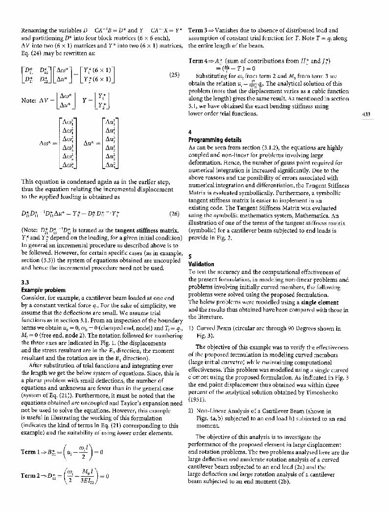
3.3 Example problem Consider, for example, a cantilever beam loaded at one end by a constant vertical force qv For the sake of simplicity, we assume that the deflections are small. We assume trial functions as in section 3.1. From an inspection of the boundary terms we obtain u 0 = 0, coo = 0 (clamped end, nodel) and T t = qt, M t = 0 (free end, node 2). The notation followed for numbering the three axes are indicated in Fig. 1. (the displacements and the stress resultant are in the E 2 direction, the moment resultant and the rotation are in the E 1 direction).

After substitution of trial functions and integrating over the length we get the below system of equations. Since, this is a planar problem with small deflections, the number of equations and unknowns are fewer than in the general case (system of Eq. (21)). Furthermore, it must be noted that the equations obtained are uncoupled and Taylor's expansion need not be used to solve the equations. However, this example is useful in illustrating the working of this formulation (indicates the kind of terms in Eq. (21) corresponding to this example) and the suitability of using lower order elements.

( coll'~ Terml = u,-T)=0

T e r m 2 ~ D ~ = (2z M ~ 3EI22/

Term 3 ~ Vanishes due to absence of distributed load and assumption of constant trial function for T. Note T = qz along the entire length of the beam.

Term 4 ~ A ~ (sum of contributions from H2* and 12") = (_~o_ T) = 0

Substituting for co I from term 2 and M 0 from term 3 we 13

obtain the relation u I = ~ qv The analytical solution of this problem (note that the displacement varies as a cubic function along the length) gives the same result. As mentioned in section 3.1, we have obtained the exact bending stiffness using lower order trial functions.

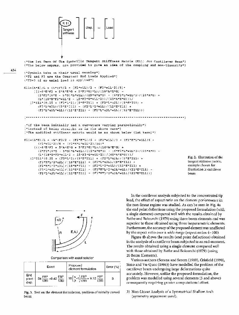
4 Programming details As can be seen from section (3.1.2), the equations are highly coupled and non-linear for problems involving large deformation. Hence, the number of gauss point required for numerical integration is increased significantly. Due to the above reasons and the possibility of errors associated with numerical integration and differentiation, the Tangent Stiffness Matrix is evaluated symbollically. Furthermore, a symbollic tangent stiffness matrix is easier to implement in an existing code. The Tangent Stiffness Matrix was evaluated using the symbollic mathematics system, Mathematica. An illustration of one of the terms of the tangent stiffness matrix (symbolic) for a cantilever beam subjected to end loads is provide in Fig. 2.

5 Validation To test the accuracy and the computational effectiveness of the present formulation, in modeling non-linear problems and problems involving initially curved members, the following problems were solved using the proposed formulation. The below problems were modelled using a single element and the results thus obtained have been compared with those in the literature.

1) Curved Beam (circular arc through 90 Degrees shown in Fig. 3).

The objective of this example was to verify the effectiveness of the proposed formulation in modeling curved members (large initial curvatre) while maintaining computational effectiveness. This problem was modelled using a single curved element using the proposed formulation. As indicated in Fig. 3 the end point displacement thus obtained was within three percent of the analytical solution obtained by Timoshenko (1951).

2) Non-Linear Analysis of a Cantilever Beam (shown in Figs. 4a, b) subjected to an end load b) subjected to an end moment.

The objective of this analysis is to investigate the performance of the proposed element in large displacement and rotation problems. The two problems analysed here are the large deflection and moderate rotation analysis of a curved cantilever beam subjected to an end load (2a) and the large deflection and large rotation analysis of a cantilever beam subjected to an end moment (2b).

433

Tangent is = oa stiffness

434

[~T~e Is. Term Of The Syrabollic Tangent Stiffness Matrix (KII) For Cantilever Beam*

(*The below exprns, are provided to give an idea of the coupling and non-linearity*

("Symbols take on their usual meaning")

("F2 and F3 are the Constant End Loads Applied*)

(*F3=0 if no axial load is applied*)

KII=(A*E)/L + (A*(E3/2 - (F2"wlL)/3 - (F3*wlL^2)/8) *

(((-6*E'F3 + 5*A*E*G + 5*F3*G)*L)/(10=A*E*G) +

(2*F2*(6*E - 5*G)*L"wlL)/(15*A'E*G) - (6*F2"L*wlL^3)/(25"A'G) +

(L*(18*E*F3*wlL^2 - !5-F3-G*~!L^2))/(40*A*E*G)))/

(3"!11"(0.25 § (F3~L^2)/(9*E*ill) + (F2"L*u2L)/(9*E"III) +

(F3*L*u3L)/(9*E'Ill) (F2*L~2*wlL)/(12"E*lll) +

(F3"L"u2L"wlL)/(12*E*!ll) - (F2~L"u3L*wlL)/(12*E"Ill)))

*If the beam initially had a curvature varying parabolical!y')

"instead of being straight as in the above case*)

"The modified stiffness matrix would be as shown below (is. term)*)

KIL=(A"E)/L + (A*(F3/2 - (F2*K*L)/5 - (F2"wlL)/3 - (F3*K~L'wLL)/6 -

(F3"~LL^2)/8 § (F2*K*L*wlL^2)/14) *

(((-6"E'F3 e 5*A"E*G + 5*F3*G)*L)/(10"A*E"G) +

(2*F2*(6*E - 5*G)*L*wlL)/(15*A*E*G) - (6"F2*L*wIL^3)/(25*AtG) +

(L*(18*E-F3*wlL^2 - 15-F3-G*wlLA2))/(40*A*E*G)))/

(3"IIi'(0.25 + (F3*LA2)/(9"E"III) + (F2"L'u2L)/(9"E'Ill) +

(F3"K*L^2"u2L)/(!8"E"II1) + (F3*L*u3L)/(9*E*!ll) -

(F2*K'L^2"u3L)/(18*E*Ill) (F2*L^2*wlL)/(12*E*lll) +

(F3*L'u2L"wlL)/(12*E*II1) (F2*K*L^2"u2L*wlL)/(21*E*~ll) -

(F2*L*u3L*wlL)/(12*E*!ll) - (F3~K*L^2*u3L*wlL)/(21*E*Ill)))

Fig. 2. Illustration of the tangent stiffness matrix, example chosen for illustration is cantilever beam

, t it

F

Comparison with exact solution

Exact

End point 37t FR3 =9 42 FR3

1251 " dlsp.

Proposed Error (%) element formulation

16(~;-1/FR3 = 9.12 FR~ 3 3 ~2 /12EI 12EI

Fig. 3. Test on the element formulation, problem of initially curved beam

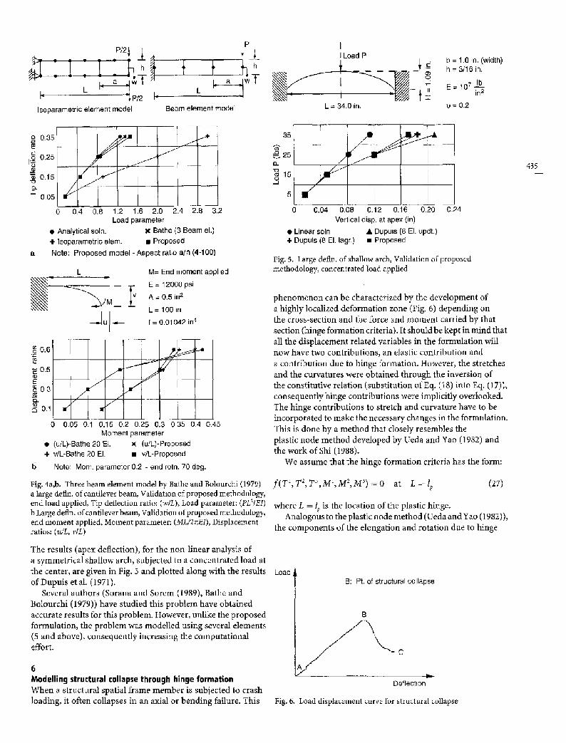
In the cantilever analysis subjected to the concentrated tip load, the effect of aspect ratio on the element performance in the non-linear regime was studied. As can be seen in Fig. 4a the end point deflections using the proposed formulation (with a single element) compared well with the results obtained by Bathe and Bolourchi (1979) using three beam elements and was superior to those obtained using three isoparametric elements. Furthermore, the accuracy of the proposed element was unaffected by the aspect ratio over a wide range (aspect ratios 4-100).

Figure 4b shows the results (end point deflections) obtained in the analysis of a cantilever beam subjected to an end-moment. The results obtained using a single element compared well with those obtained by Bathe and Bolourchi (1979) (using 20 Beam Elements).

Various authors (Sorana and Sorem (1989), Crisfield (1990), Simo and Vu-Quoc (1986)) have modelled the problem of the cantilever beam undergoing large deformations quite accurately. However, unlike the proposed formulation, the problem was modelled using several elements (5 and above) consequently requiring greater computational effort.

3) Non-Linear Analysis of a Symmetrical Shallow Arch (symmetry arguement used).

- ;. - j w f , a L r ~

P/2 I" L I, v

Isoparametric element model Beam element model

I I Load P

L = 34.0 in.

b = 1.0 in. (width) h = 3/16 in,

E= 107 113 in 2

0=0.2

o 0.35

0.15 "O

~- 0.05

f ) . f J

r 0 0.4 0.8 1.2 1.6 2.0 2.4 2.8 3.2

Load parameter �9 Analytical soln. X Bathe (3 Beam el.) § Isoparametric elem. �9 Proposed Note: Proposed model - Aspect ratio a/h (4-100)

M= End moment applied

E = 12000 psi

A = 0.5 in 2

L = 100 in

I = 0.01042 in 4

0.6

E 0.5

E 0,3

c~ 0.1

Y / /

m/

/ /

I

j l f , / J

0 0.05 0.1 0.15 0.2 0.25 0.3 035 0.4 0.45 Moment parameter

�9 (u/L)-Bathe 20 El. x (u/L)-Proposed § v/L-Bathe 20 El. �9 v/L-Proposed

Note: Morn. parameter 0.2 - end rotn. 70 deg.

Fig. 4a,b. Three beam element model by Bathe and Bolourchi (1979) a large defln, of cantilever beam, Validation of proposed methodology, end load applied, Tip deflection ratio: (w/L), Load parameter: (PL21EI) b Large defln, of cantilever beam, Validation of proposed methodology, end moment applied, Moment parameter: (ML/2zcEI), Displacement ratios: (u/L, v/L)

~" 3 5

----- 25

~ 15

0 0.04 0.08 0.12 0.16 0.20 0.24 Vertical disp. at apex (in)

�9 Linear soln �9 Dupums (8 El. updt.) § Dupuis (8 El. lagr.) �9 Proposed

Fig. 5. Large defln, of shallow arch, Validation of proposed methodology, concentrated load applied

phenomenon can be characterized by the development of a highly localized deformation zone (Fig. 6) depending on the cross-section and the force and moment carried by that section (hinge formation criteria). It should be kept in mind that all the displacement related variables in the formulation will now have two contributions, an elastic contribution and a contribution due to hinge formation. However, the stretches and the curvatures were obtained through the inversion of the constitutive relation (substitution of Eq. (18) into Eq. (17)), consequently hinge contributions were implicitly overlooked. The hinge contributions to stretch and curvature have to be incorporated to make the necessary changes in the formulation. This is done by a method that closely resembles the plastic node method developed by Ueda and Yao (1982) and the work of Shi (1988).

We assume that the hinge formation criteria has the form:

f(T1, T2, T3,M1,M2,M3)=O at L=lp (27)

where L = lp is the location of the plastic hinge. Analogous to the plastic node method (Ueda and Yao (1982)),

the components of the elongation and rotation due to hinge

435

The results (apex deflection), for the non-linear analysis of a symmetrical shallow arch, subjected to a concentrated load at the center, are given in Fig. 5 and plotted along with the results of Dupuis et al. (1971).

Several authors (Sorana and Sorem (1989), Bathe and Bolourchi (1979)) have studied this problem have obtained accurate results for this problem. However, unlike the proposed formulation, the problem was modelled using several elements (5 and above), consequently increasing the computational effort.

6 Modelling structural collapse through hinge formation When a structural spatial frame member is subjected to crash loading, it often collapses in an axial or bending failure. This

Load T B: Pt. of structural collapse

/ B

Deflection

Fig. 6. Load displacement curve for structural collapse

436

formation may be written as:

( e , ) z ~ = ) o ~ at L = I p

(0i)zp=~ ~f at L = l p ; i = 1 , 2 , 3 (28)

where the plastic hinge parameter 2 and the hinge formation criteria shall be determined through numerical experiments performed on DYNA3D.

It is worth recalling here that the curvature vector is defined as the derivative of the tangent vector with respect to the arc length parameter. Hence, it can be seen that though the curvature becomes singular in the vicinity of the hinge, its integral over the length in this region is just the change in slope across the hinge. Let us denote the rotation vector corresponding to hinge rotations by R v (It is important to note that the curvature far away from the hinge is unaffected by the hinge formation). In a similar fashion, the integral of the hinge contribution of the stretch gives the elongation.

It can be shown that on accounting for the hinge contributions of stretch and curvature results in the following additional terms in condition (17).

- - ~ST.R .e/1 p - c~M.R .Rp/tp (29)

7

Conclusion The developments accomplished in the present course of study are listed below:

A frame element formulation that is capable of."

a) handling large rotations and displacements; and the effect of transverse shear

b) modelling structural collapse through hinge formation c) modeling members with initial curvature d) running on a high and P.C. or equivalent computational

resource has been developed. Based on the validation for geometrically non-linear problems and initially curved members, it is expected that only one element will be required per member for modeling crash scenarios.

From the frame kinematics (Section 2.1) it can be seen that the formulation handles large deflections, rotations and can be used for members with initial curvature. It can also be seen from section (5) that lower order elements can be used with only one element per frame span (Section 3.3) thus greatly enhancing computational effeciency. It should also be noted here that because of the generality of the present formulation, a family of simplified elements may be derived by dropping terms like change in curvature, initial curvature etc.

Structural collapse is handled through hinge formation (Sect. 6). As indicated in Fig. 6, the structural collapse is characterized by a sudden drop in the load-deflection curve (Portion B-C in Fig. 2). In the formulation developed, hinge formation (point B) is determined by Eq. (27). When this equation is satisfied the additional terms due to hinge formation are incorporated (using Eqs. (28) and (29)). This results in lowering of structural stiffness characterized by a sudden increase in deformation and the consequent decrease in stress and moment resultants.

References Afluri, S. N.; Murakawa, H. 1977: On hybrid-finite element models in nonlinear solid mechanics. Finite elements in nonlinear mechanics. Vol. 1, 3-41 Tapir Press Afluri, S. N. 1984: Alternate stress and conjugate strain measures, and mixed variational formulations involving rigid rotations, for computational analyses of finitely deformed solids, with applications to plates and shells-I, theory. Computers and Structures. 18, No. 1: 93-116 Afluri, S. N.; Cazani, A. 1995: Rotations in computational solid mechanics. Archives for Computational Methods in Engg., Vol. 2, No. 1: 49-138 Bathe, K. l.; Bolourchi, S. 1979: Large displacement analysis of three-dimensional beam structures. Int. Journal for Num. Methods in Engg., Vol. 14:961-986 Cowper, G. R. 1966: The shear coeffecient in Timoshenko's beam theory. J. Appl. Mech. 33:335-340 Crisfield, M. A. 1990: A consistent co-roatational formulation for non-linear, three dimensional, beam-elements. Computer Methods in Appl. Mech. and Engg., 81:131-150 Dupuis, G. A.; Hibitt, H. D.; McNamara, S. F.; Marcal, P. V. 1971: Nonlinear material and geometric behavior of shell structures. Computers and Structures. Vol. 1:223-239 Fraejis de Veubeke, B. 1972: A new variational principle for finite elastic displacements. Int. Journal of Engg. Sci. 10: 745- 763 Iura, M.; Afluri, S. N. 1988: A dynamic analysis of finitely stretched and rotated three-dimensional space-curved beams. Computers and Structures. VoI. 29, No. 5:875-889 Iura, M.: Afluri, S. N. 1989: On a consistent theory, variational formulation of finitely stretched and rotated 3-D space-curved beams. Computational Mechanics. 4: 73- 88 Pietraskiewicz, W.; Badur, J. 1983: Finite rotations in the description of continuum deformation. Int. J. Eng. Sci. 21, No. 9: 1097-1115 Shi, G. 1988: Nonlinear static and dynamic analyses of large-scale lattice-type structures and nonlinear active control by piezo actuators. Ph.D. Thesis (Advisor, Dr. Atluri, S. N., School of Civil Engg. Georgia Inst. of Tech.) Simo, J. C.; Vu-Quoc, L. 1986: A three-dimensional finite strain model. Part 2: (computational aspects). Computer Methods in Appl. Mech. and Engg., 58:79-116 Surana, K. S.; Sorem, R. M. 1989: Geometrically non-linear formulation for three dimensional curved beam elements with large rotations. Int. Journal for Num. Methods in Engg., Vol. 28:43-73 Timoshenko 1951: Theory of Elasticity, third edition. 83- 87