Deterministic versus Stochastic Design of Water Distribution Networks

Dow

nloa

ded

from

asc

elib

rary

.org

by

UN

IVE

RSI

TY

OF

VIR

GIN

IA o

n 06

/16/

14. C

opyr

ight

ASC

E. F

or p

erso

nal u

se o

nly;

all

righ

ts r

eser

ved.

Deterministic versus Stochastic Designof Water Distribution Networks

Orazio Giustolisi1; Daniele Laucelli2; and Andrew F. Colombo3

Abstract: The paper describes a procedure for the robust design of water distribution networks which incorporates the uncertainty ofnodal water demands and pipe roughness in a multiobjective optimization scheme aimed at minimizing costs and maximizing hydraulicreliability. The methodology begins with a deterministic system design in order to generate a set of optimal networks that serves as theinitial population for subsequent multiobjective stochastic design. This approach does not depend on the choice of multiobjectiveoptimizer �for example, a multiobjective genetic algorithm is used here� and can drastically reduce the number of “stochastic” runs neededfor searching robust solutions. A collection of probability density functions based on the � function is introduced and applied to modelingvariable uncertainty according to different physical requirements. The approach is tested in a case study involving a real network,illustrating its computational advantages.

DOI: 10.1061/�ASCE�0733-9496�2009�135:2�117�

CE Database subject headings: Stochastic processes; Water distribution systems; Networks; System reliability; Uncertaintyprinciples.

Introduction

Risk-based management of water distribution systems �WDS� en-courages utilities to perceive reliability assessment as a usefultool for achieving effective management of new and existing net-works. Walski �2001� stressed the need for developing new net-work design strategies, not only for addressing the minimizationof pipe costs, but also the maximization of network reliability.This is usually interpreted as the provision of nodal head in ex-cess of that which is established as a minimum within the net-work. The term “reliability” can be thought of as a system’sability to demonstrate adequate performance during both normaland unusual operating conditions �Xu and Goulter 1999� and isusually studied by considering two general classes of failures�Farmani et al. 2005�: mechanical and hydraulic. The former re-fers to system component failure �such as pipe breaks, blockage,valve immobilization, pumping station interruptions, etc.�, whoseoccurrence depends on appurtenance and device reliability and isthus closely related to rehabilitation/maintenance plans. Hydraulicfailure refers to unforeseen alterations in nodal demands and piperoughness, or in the inability to cope effectively with these.

Change in nodal demands often unfolds simultaneously withcapacity deterioration due to aging and either process can result in

1Professor Dean, Engineering Faculty of Taranto, Dept. of Civil andEnvironmental Engineering, Technical Univ. of Bari, via le del Turismo,8, 74100 Taranto, Italy �corresponding author�. E-mail: [email protected]

2Research Fellow, Dept. of Civil and Environmental Engineering,Technical Univ. of Bari, v. E. Orabona 4, 70123 Bari, Italy.

3Visiting Research Fellow, Engineering Faculty of Taranto, v. le delTurismo 8, Technical Univ. of Bari, 74100 Taranto, Italy.

Note. Discussion open until August 1, 2009. Separate discussionsmust be submitted for individual papers. The manuscript for this paperwas submitted for review and possible publication on April 12, 2007;approved on August 11, 2008. This paper is part of the Journal of WaterResources Planning and Management, Vol. 135, No. 2, March 1, 2009.
©ASCE, ISSN 0733-9496/2009/2-117–127/$25.00.
JOURNAL OF WATER RESOURCES P

J. Water Resour. Plann. Mana

pressure at one or more nodes falling below an acceptable level.Babayan et al. �2005� defined “robustness of the network” as theability to adequately supply customers despite fluctuations insome, or all, of the design parameters �i.e., nodal demands, piperoughness, etc.�. Network robustness is dependent on the variabil-ity and cross correlations �Farmani et al. 2005� assumed for nodaldemands and pipe roughness �Lansey et al. 1989; Xu and Goulter1999; Babayan et al. 2005; Kapelan et al. 2005�. Thus, the designchallenge is to develop a strategy able to produce dependableresults when faced with uncertainty �that is, incorporating robust-ness into the design approach�. The stochastic least-cost WDSdesign problem was first conceived and solved as a single-objective formulation by Lansey et al. �1989�. It was then inter-preted as a constrained minimization problem and solved usingthe generalized reduced gradient 2 �GRG2� technique. Xu andGoulter �1999� developed an approach in which the first-orderreliability method �FORM� was used and the optimization wasperformed by GRG2. Calculations proved too laborious and themethod was time consuming even for small networks �Savic2004�. Moreover, the GRG2 optimization procedure assumes thedecision variables �i.e., pipe diameters� as continuous, which isunrealistic. Tolson et al. �2004� tried to improve this approachcombining a genetic algorithm �GA�-based optimization schemewith a method for estimating WDS reliability based on FORM.The approach necessitates repetitive calculation of the first-orderderivatives and matrix inversions in order to calculate uncertain-ties and becomes computationally demanding even for small net-works, sometimes inviting numerical problems. Babayan et al.�2005� avoided recourse to a sampling-based method using singleobjective GA linked to an integration-based uncertainty quantifi-cation technique. They assumed some probability density func-tions for nodal demand fluctuations �uncertainty� and defined a setof critical nodes �i.e., those that did not satisfy pressure require-ments� which were used for the evaluation of the fitness function.However, the actual level of robustness cannot be specified ex-plicitly in the problem formulation, but is calculated once the
optimization process has converged to the final solution. The
LANNING AND MANAGEMENT © ASCE / MARCH/APRIL 2009 / 117

ge. 2009.135:117-127.

Dow

nloa

ded

from

asc

elib

rary

.org

by

UN

IVE

RSI

TY

OF

VIR

GIN

IA o

n 06

/16/

14. C

opyr

ight

ASC

E. F

or p

erso

nal u

se o

nly;

all

righ

ts r

eser

ved.

above-mentioned stochastic WDS design methodologies have onecommon limitation: optimization is formulated and solved as aconstrained single-objective problem, thus resulting in a singleoptimal solution.

Recently, Kapelan et al. �2005� proposed a multiobjective�MO� optimization approach for solving WDS design under un-certainty. They modeled the uncertain variables �i.e., nodal de-mands and pipe roughness� by means of normal and uniformprobability density functions �PDFs�, respectively, which are cal-culated using the Latin hypercube �LH� sampling technique�McKay et al. 1979�. The chosen method is the Robust NSGAII,which is based on the nondominated Sorting Genetic Algorithm II�NSGAII� �Deb et al. 2002�. The procedure exploits a small num-ber of samples for fitness evaluation, leading to significant com-putational savings and producing a robust Pareto optimal front ofsolutions.

This paper proposes a multiobjective approach to the WDSdesign problem, considering nodal demands and pipe roughnessas uncertain variables. The optimal design procedure is conceivedand formulated for use with an optimizer based on a standard GA.In particular, the optimized multiobjective genetic algorithm �OP-TIMOGA�, as in Giustolisi et al. �2004�, is featured. The pro-posed strategy performs a deterministic design �i.e., constrainedleast-cost design procedure� as the first step and then, using thedeterministic solutions as initial population, solves the robust de-sign problem multiobjectively, implementing the minimization ofdesign costs and the maximization of WDS robustness as objec-tive functions. As explained subsequently, this approach can offersignificant computational savings. Further, network robustness isdefined based on the worst-performing �i.e., critical� node, afterthe evaluation of hydraulic performances of all the networknodes. Finally, a collection of PDFs is tested with the goal ofmodeling system uncertainty in different ways. Save for the nor-mal distribution, they are all based on the � function �Mood et al.1974� with each applied PDF being defined on a bounded domainand evaluated for a different range. The methodology is verifiedin a case study of a real planned network for an industrial area inan Apulian town �Southern Italy�.

Network Simulation Model for Pipe Sizing

The paper assumes the demand-driven formulation given in To-dini and Pilati �1988�. However, it should be recalled that nodaldemands are usually treated as constants for each simulation evenif, in reality, they change. To reflect this, their fluctuations arehere accounted for by some representative PDF �Kapelan et al.2005; Babayan et al. 2005; Giustolisi et al., 2005�. Therefore, anetwork comprising np pipes carrying unknown flows, nn nodeswith unknown pressure heads, and n0 nodes with known pressurehead �reservoirs� can be described as follows:

�App Apn

Anp 0��Q

H� = �− Ap0H0

q� �1�

where Q= �Q1 ,Q2 , . . . ,Qnp�T= �np ,1� column vector of the com-puted pipe flows; H= �H1 ,H2 , . . . ,Hnn�T= �nn ,1� column vectorof the computed nodal total heads; H0= �H01 ,H02 , . . . ,H0n0�T

= �n0 ,1� column vector of the known nodal total heads; and q= �q1 ,q2 , . . . ,qnn�T= �nn ,1� column vector of the nodal demands,which here are assumed to vary according to some PDF.

In the mathematical system �1�, App represents a �np ,np� diag-n−1
onal matrix whose elements are defined as App�i , i�=Ri�Qi� ,
118 / JOURNAL OF WATER RESOURCES PLANNING AND MANAGEMENT


whereas Apn=AnpT and Ap0 are topological incidence submatrices,

of size �np ,nn� and �np ,n0�, respectively, derived from the general

topological matrix Apn= �Apn �Ap0� of size �np ,nn+n0�, defined asin Todini and Pilati �1988�. Ri is the pipe hydraulic resistance thatis a function of pipe roughness, diameter, and length, whereas n isan exponent which takes into account the actual flow regime andadopted head loss relationship �here n=2 is used�. In this work,pipe roughness �and thus pipe hydraulic resistance Ri� is assumedto vary according to some PDF.

Single-Objective Optimization

The classical problem of network design centers on the selectionof pipe diameters, given the pressure head at nodes H, computedfrom system �1� for fixed deterministic demands and roughness�dependent on diameters�, and it is constrained by a minimumnodal pressure head for supplying demand. The problem is usu-ally formulated with a single objective: minimum pipe cost. Forinstance, system �1� is typically completed with the followingequations �Savic and Walters 1997�:

f�D1,D2, . . . ,Dnp� = �

i=1

np

C�Di,Li� → min �2�

Hj � Pjmin + Zj, j = 1, . . . ,nn �3�

where the former deals with financial cost minimization �depen-dent on pipe diameter �Di� and length �Li�� and the latter pertainsto service level constraints �Pj

min is the minimum nodal pressurehead and Zj its elevation above datum� that must be satisfied inorder to supply required nodal demands. Thus, pipe diameters arethe decision variables of the optimization problem and their ap-propriate selection is the specific goal of the design task. Theformulation in Eqs. �1�–�3� leads to a complex �nonlinear� com-binatorial optimization environment as diameter choices are dis-crete. Savic and Walters �1997� demonstrated that GA are anefficient way to solve this kind of problem as they undertake awide exploration of the solution space, implying a high probabil-ity of exposing the global optimum.

Robust WDS Design and Multiobjective Formulation

Recently, Kapelan et al. �2005� proposed a MO optimization ap-proach for solving WDS design under uncertainty. They modeledthe uncertain variables �i.e., nodal demands and pipe roughness�by means of Gaussian and uniform PDFs, assuming some corre-lation among the samples used. The LH technique was applied tocalculate the PDFs in order to reduce the number of samples �atleast equal to 30 for each individual in each generation�. How-ever, the key element in this work lies in the optimization method.They used the robust NSGAII, based on the NSGAII �Deb et al.2002�, which is able to evaluate each individual’s fitness, spread-ing the sampling over a number of generations. The objectivefunctions were pipe cost minimization and network robustnessmaximization, which is computed as the fraction �i.e., percentage�of the total number of samples for which the minimum pressurehead requirement is met simultaneously at all nodes in the net-work. The methodology produces a robust Pareto front of optimalsolutions which is then subjected to a final validation by applyinga Monte Carlo �MC� simulation to the optimal solutions and de-
leting those that turn out to be dominated after the final check.
© ASCE / MARCH/APRIL 2009

ge. 2009.135:117-127.

Dow

nloa

ded

from

asc

elib

rary

.org

by

UN

IVE

RSI

TY

OF

VIR

GIN

IA o

n 06

/16/

14. C

opyr

ight

ASC

E. F

or p

erso

nal u

se o

nly;

all

righ

ts r

eser

ved.

The procedure makes use of a small number of samples for fitnessevaluation, leading to significant computational savings if com-pared to the full sampling approach �the procedure without thefinal MC simulations takes at least 27 min to return the Paretofront�.

Proposed Approach

This paper introduces an alternative to the procedure of Kapelanet al. �2005� which involves the development and testing of arobust MO design strategy for WDS design employing a generalpurpose MO genetic algorithm �MOGA� as optimizer �OPTI-MOGA, Giustolisi et al. 2004�. The innovative aspects of theprocedure with respect to recent contributions �Kapelan et al.2005; Babayan et al. 2005; Tolson et al. 2004� include:1. The use of a set of � PDFs �Giustolisi et al. 2005� in order to

model nodal demand and roughness uncertainties with somevariety. This permits incorporation of a bounded PDF, which,coupled with the LH sampling technique, can allow a betterrandom sample stratification leading to more accurate esti-mation of the empirical, nodal head PDF tails �Mood et al.1974; Fishman 1996�, which is important when evaluatingWDS design robustness. Moreover, the proposed tests on realdata of different PDFs �including the normal� can show thetechnical consistency of � PDFs, allowing engineers tochoose from among them, according to their own knowledgeand experience, those best suited to represent the features ofuncertain parameters. The normal PDF is here defined on abounded domain in order to avoid numerical and physicalproblems related to its original unbounded properties.

2. The evaluation of robustness of each optimal design solutionis made with respect to the network’s critical node �i.e., theworst-performing node�, as the probability that its stochasticnodal head �Hj� is higher than the service level �Pj

min+Zj�,assuming the conservative hypothesis that the nodal headscould vary according to a normal PDF. Thus, robustnessmaximization is an objective function integrated in the opti-mization procedure, whereas in previous works it is usuallycalculated at the end of single-objective optimization. Assubsequently clarified, the features of the analyzed network�i.e., few nodes, similar water demands, etc.� allow for theevaluation of network robustness with reference to the criti-cal node without compromising the procedure’s efficiency.Larger and more complex networks might need a third ob-jective function looking at a number of critical nodes or criti-cal zones �not contiguous critical nodes� which can beaffected by service failures.

3. The design procedure is twofold: first, the problem is solvedwithin the context of a least-cost deterministic approachusing the minimization of costs and pressure deficit on thenetwork’s critical node as objective functions; second, robustdesign is performed as a dual-objective optimization problem�cost versus network robustness� employing the deterministicsolutions as an initial population. This assumption, to beclarified subsequently, is justified by evidence that the deter-ministic solutions �i.e., network configurations� are close to,or at least belong to, the final Pareto front of robust/stochastic solutions. The robust design phase uses the mini-mization of costs and the maximization of networkrobustness as objective functions. Overall, the entire ap-
proach can significantly reduce computational effort.


Nodal Demand and Pipe Roughness Uncertainty

Traditionally, both nodal demands qj and pipe hydraulic resis-tance Ri have been treated as fixed and known parameters fordesign and performance evaluation. Clearly, this is not ideal asthe values of these parameters are not usually known with accu-racy, especially when entertaining long-term projections. To over-come this challenge, all future nodal demands and roughnessparameters will be treated as uncertain variables whose values aregoverned by a PDF and, to simplify things, no correlation be-tween any two random variables will be modeled �Kapelan et al.2005�. However, generally speaking, correlation among nodal de-mands can be assumed, for example, due to some extent on un-certain factors that affect the system as a whole, such as hot, dryweather, which can result in significant extra consumption �i.e.,garden watering, drinking, etc.�, thus increasing or decreasing de-mand at all nodes simultaneously �Kapelan et al. 2005�. Assuminga normal PDF with unit mean and standard deviation �, i.e.,N�1,��, the following can be written for nodal demands and piperoughness:

qjunc � N�qj,� jqj� = qjN�1,� j�

�4�Ri

unc � N�Ri,�iRi� = RiN�1,�i�

In Eq. �4�, the N�1,�� PDF plays the role of a proportionalitycoefficient for the uncertain variables �i.e., � is related to therelative uncertainty level of the corresponding variable�. Uncer-tainty quantification is performed here using the sampling ap-proach based on MC methodology. Specifically, the LH techniqueis employed as the variance reduction method for limiting thenumber of samples required. To avoid consideration of unrealisticextreme values in the case of a normal PDF, a special beta PDF isused �Giustolisi et al. 2005�

��a,b� =xa−1�1 − x�b−1

beta�a,b��5�

where ��a ,b� stands for the beta PDF with parameters a and b,and beta �a ,b� is the beta function �Mood et al. 1974�. In Eq. �5�,the value of the beta PDF is defined for x in the range �0, 1�. Thevalues of a and b can be chosen so that the probability distribu-tion has the required mean value m and standard deviation �

m =a

a + b�6�

� = �a + b�−1 ab

�a + b + 1�

By manipulating the values of a and b, the beta PDF can beused to generate different types of PDF bounded in a range that isdefined by the user. The idea of assuming the shape, mean, andrange �in spite of the standard deviation� of the PDF is technicallysound. PDFs of different shape can be related to informationabout uncertainty and the variable’s range is an easier parameterto select. Thus, four beta PDFs have been constructed with thesame standard deviation, deriving from a particular normal PDF.This paper takes into consideration the distribution N�0.5,��,where � is computed so that the normal PDF is constrained to therange �0, 1�, for example, the upper and lower limits correspond-ing to the cumulative values of 0.001 and 0.999. In this way, thestandard deviation of the normal PDF is equal to ��=m /3.0902�⇒ �0.1618=0.5 /3.0902�, with 3.0902 being the value
associated with the cumulative PDF at 0.999. By Eq. �6�, the

ge. 2009.135:117-127.

Dow

nloa

ded

from

asc

elib

rary

.org

by

UN

IVE

RSI

TY

OF

VIR

GIN

IA o

n 06

/16/

14. C

opyr

ight

ASC

E. F

or p

erso

nal u

se o

nly;

all

righ

ts r

eser

ved.

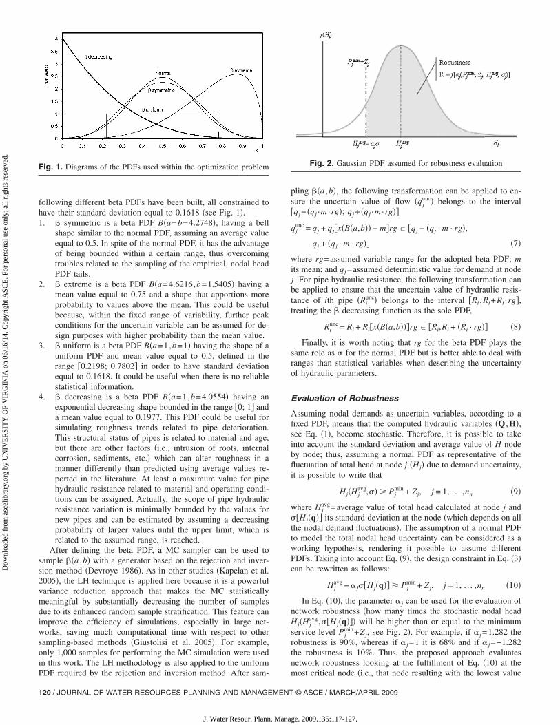
following different beta PDFs have been built, all constrained tohave their standard deviation equal to 0.1618 �see Fig. 1�.1. � symmetric is a beta PDF B�a=b=4.2748�, having a bell

shape similar to the normal PDF, assuming an average valueequal to 0.5. In spite of the normal PDF, it has the advantageof being bounded within a certain range, thus overcomingtroubles related to the sampling of the empirical, nodal headPDF tails.

2. � extreme is a beta PDF B�a=4.6216,b=1.5405� having amean value equal to 0.75 and a shape that apportions moreprobability to values above the mean. This could be usefulbecause, within the fixed range of variability, further peakconditions for the uncertain variable can be assumed for de-sign purposes with higher probability than the mean value.

3. � uniform is a beta PDF B�a=1,b=1� having the shape of auniform PDF and mean value equal to 0.5, defined in therange �0.2198; 0.7802� in order to have standard deviationequal to 0.1618. It could be useful when there is no reliablestatistical information.

4. � decreasing is a beta PDF B�a=1,b=4.0554� having anexponential decreasing shape bounded in the range �0; 1� anda mean value equal to 0.1977. This PDF could be useful forsimulating roughness trends related to pipe deterioration.This structural status of pipes is related to material and age,but there are other factors �i.e., intrusion of roots, internalcorrosion, sediments, etc.� which can alter roughness in amanner differently than predicted using average values re-ported in the literature. At least a maximum value for pipehydraulic resistance related to material and operating condi-tions can be assigned. Actually, the scope of pipe hydraulicresistance variation is minimally bounded by the values fornew pipes and can be estimated by assuming a decreasingprobability of larger values until the upper limit, which isrelated to the assumed range, is reached.

After defining the beta PDF, a MC sampler can be used tosample ��a ,b� with a generator based on the rejection and inver-sion method �Devroye 1986�. As in other studies �Kapelan et al.2005�, the LH technique is applied here because it is a powerfulvariance reduction approach that makes the MC statisticallymeaningful by substantially decreasing the number of samplesdue to its enhanced random sample stratification. This feature canimprove the efficiency of simulations, especially in large net-works, saving much computational time with respect to othersampling-based methods �Giustolisi et al. 2005�. For example,only 1,000 samples for performing the MC simulation were usedin this work. The LH methodology is also applied to the uniform

Fig. 1. Diagrams of the PDFs used within the optimization problem

PDF required by the rejection and inversion method. After sam-



pling ��a ,b�, the following transformation can be applied to en-sure the uncertain value of flow �qj

unc� belongs to the interval�qj − �qj ·m ·rg�; qj + �qj ·m ·rg��

qjunc = qj + qj�x�B�a,b�� − m�rg � �qj − �qj · m · rg�,

qj + �qj · m · rg�� 7�

where rg=assumed variable range for the adopted beta PDF; mits mean; and qj =assumed deterministic value for demand at nodej. For pipe hydraulic resistance, the following transformation canbe applied to ensure that the uncertain value of hydraulic resis-tance of ith pipe �Ri

unc� belongs to the interval �Ri ,Ri+Ri ·rg�,treating the � decreasing function as the sole PDF,

Riunc = Ri + Ri�x�B�a,b��rg � �Ri,Ri + �Ri · rg�� 8�

Finally, it is worth noting that rg for the beta PDF plays thesame role as � for the normal PDF but is better able to deal withranges than statistical variables when describing the uncertaintyof hydraulic parameters.

Evaluation of Robustness

Assuming nodal demands as uncertain variables, according to afixed PDF, means that the computed hydraulic variables �Q ,H�,see Eq. �1�, become stochastic. Therefore, it is possible to takeinto account the standard deviation and average value of H nodeby node; thus, assuming a normal PDF as representative of thefluctuation of total head at node j �Hj� due to demand uncertainty,it is possible to write that

Hj�Hjavg,�� Pj

min + Zj, j = 1, . . . ,nn �9�

where Hjavg=average value of total head calculated at node j and

��Hj�q�� its standard deviation at the node �which depends on allthe nodal demand fluctuations�. The assumption of a normal PDFto model the total nodal head uncertainty can be considered as aworking hypothesis, rendering it possible to assume differentPDFs. Taking into account Eq. �9�, the design constraint in Eq. �3�can be rewritten as follows:

Hjavg − � j��Hj�q�� Pj

min + Zj, j = 1, . . . ,nn �10�

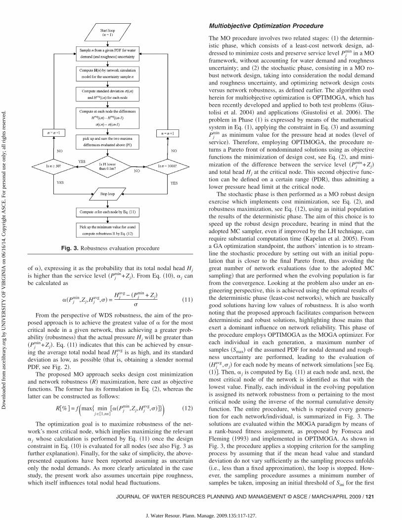
In Eq. �10�, the parameter � j can be used for the evaluation ofnetwork robustness �how many times the stochastic nodal headHj�Hj

avg ,��Hj�q�� will be higher than or equal to the minimumservice level Pj

min+Zj, see Fig. 2�. For example, if � j =1.282 therobustness is 90%, whereas if � j =1 it is 68% and if � j =−1.282the robustness is 10%. Thus, the proposed approach evaluatesnetwork robustness looking at the fulfillment of Eq. �10� at the

Fig. 2. Gaussian PDF assumed for robustness evaluation

most critical node �i.e., that node resulting with the lowest value


ge. 2009.135:117-127.

Dow

nloa

ded

from

asc

elib

rary

.org

by

UN

IVE

RSI

TY

OF

VIR

GIN

IA o

n 06

/16/

14. C

opyr

ight

ASC

E. F

or p

erso

nal u

se o

nly;

all

righ

ts r

eser

ved.

of ��, expressing it as the probability that its total nodal head Hj

is higher than the service level �Pjmin+Zj�. From Eq. �10�, � j can

be calculated as

��Pjmin,Zj,Hj

avg,�� =Hj

avg − �Pjmin + Zj�

��11�

From the perspective of WDS robustness, the aim of the pro-posed approach is to achieve the greatest value of � for the mostcritical node in a given network, thus achieving a greater prob-ability �robustness� that the actual pressure Hj will be greater than�Pj

min+Zj�. Eq. �11� indicates that this can be achieved by ensur-ing the average total nodal head Hj

avg is as high, and its standarddeviation as low, as possible �that is, obtaining a slender normalPDF, see Fig. 2�.

The proposed MO approach seeks design cost minimizationand network robustness �R� maximization, here cast as objectivefunctions. The former has its formulation in Eq. �2�, whereas thelatter can be constructed as follows:

R�%� = f�max minj��1,nn�

��Pjmin,Zj,Hj

avg,�� 12�

The optimization goal is to maximize robustness of the net-work’s most critical node, which implies maximizing the relevant� j whose calculation is performed by Eq. �11� once the designconstraint in Eq. �10� is evaluated for all nodes �see also Fig. 3 asfurther explanation�. Finally, for the sake of simplicity, the above-presented equations have been reported assuming as uncertainonly the nodal demands. As more clearly articulated in the casestudy, the present work also assumes uncertain pipe roughness,

Fig. 3. Robustness evaluation procedure

which itself influences total nodal head fluctuations.



Multiobjective Optimization Procedure

The MO procedure involves two related stages: �1� the determin-istic phase, which consists of a least-cost network design, ad-dressed to minimize costs and preserve service level Pj

min in a MOframework, without accounting for water demand and roughnessuncertainty; and �2� the stochastic phase, consisting in a MO ro-bust network design, taking into consideration the nodal demandand roughness uncertainty, and optimizing network design costsversus network robustness, as defined earlier. The algorithm usedherein for multiobjective optimization is OPTIMOGA, which hasbeen recently developed and applied to both test problems �Gius-tolisi et al. 2004� and applications �Giustolisi et al. 2006�. Theproblem in Phase �1� is expressed by means of the mathematicalsystem in Eq. �1�, applying the constraint in Eq. �3� and assumingPj

min as minimum value for the pressure head at nodes �level ofservice�. Therefore, employing OPTIMOGA, the procedure re-turns a Pareto front of nondominated solutions using as objectivefunctions the minimization of design cost, see Eq. �2�, and mini-mization of the difference between the service level �Pj

min+Zj�and total head Hj at the critical node. This second objective func-tion can be defined on a certain range �PDR�, thus admitting alower pressure head limit at the critical node.

The stochastic phase is then performed as a MO robust designexercise which implements cost minimization, see Eq. �2�, androbustness maximization, see Eq. �12�, using as initial populationthe results of the deterministic phase. The aim of this choice is tospeed up the robust design procedure, bearing in mind that theadopted MC sampler, even if improved by the LH technique, canrequire substantial computation time �Kapelan et al. 2005�. Froma GA optimization standpoint, the authors’ intention is to stream-line the stochastic procedure by setting out with an initial popu-lation that is closer to the final Pareto front, thus avoiding thegreat number of network evaluations �due to the adopted MCsampling� that are performed when the evolving population is farfrom the convergence. Looking at the problem also under an en-gineering perspective, this is achieved using the optimal results ofthe deterministic phase �least-cost networks�, which are basicallygood solutions having low values of robustness. It is also worthnoting that the proposed approach facilitates comparison betweendeterministic and robust solutions, highlighting those mains thatexert a dominant influence on network reliability. This phase ofthe procedure employs OPTIMOGA as the MOGA optimizer. Foreach individual in each generation, a maximum number ofsamples �Smax� of the assumed PDF for nodal demand and rough-ness uncertainty are performed, leading to the evaluation of�Hj

avg ,� j� for each node by means of network simulations �see Eq.�1��. Then, � j is computed by Eq. �11� at each node and, next, themost critical node of the network is identified as that with thelowest value. Finally, each individual in the evolving populationis assigned its network robustness from � pertaining to the mostcritical node using the inverse of the normal cumulative densityfunction. The entire procedure, which is repeated every genera-tion for each network/individual, is summarized in Fig. 3. Thesolutions are evaluated within the MOGA paradigm by means ofa rank-based fitness assignment, as proposed by Fonseca andFleming �1993� and implemented in OPTIMOGA. As shown inFig. 3, the procedure applies a stopping criterion for the samplingprocess by assuming that if the mean head value and standarddeviation do not vary sufficiently as the sampling process unfolds�i.e., less than a fixed approximation�, the loop is stopped. How-ever, the sampling procedure assumes a minimum number of
samples be taken, imposing an initial threshold of Sini for the first

ge. 2009.135:117-127.

Dow

nloa

ded

from

asc

elib

rary

.org

by

UN

IVE

RSI

TY

OF

VIR

GIN

IA o

n 06

/16/

14. C

opyr

ight

ASC

E. F

or p

erso

nal u

se o

nly;

all

righ

ts r

eser

ved.

individual to be evaluated within a generation. Fig. 3 thenchanges dynamically during the computation of all the individualsin the population, being set to the updated number of samplesnecessary to stabilize the initial oscillations of Havg�i ,n� and��i ,n�, with respect to the assumed approximation. Despite this,the number of iterations is constrained to the range �Smin; Smax� toensure an adequate number of samples when avoiding an endlessloop. This contrivance leads to a marked reduction in the numberof iterations, eschewing useless sampling and enjoying significantcomputational benefits.

Finally, during the MOGA run, the evolving Pareto front canbe bounded between two extreme values of network robustness�R�, implying the related limit of the parameter �. This choice isdriven by the practical benefit of the returned diagrams; actually,networks having robustness beyond an upper limit can be consid-ered too expensive to warrant further consideration, whereas net-works with very low robustness should not be perceived asappreciably more reliable because they remain closely compa-rable to the deterministic solutions. In the following section, fur-ther descriptions are provided on the used limits and motivations.

Case Study

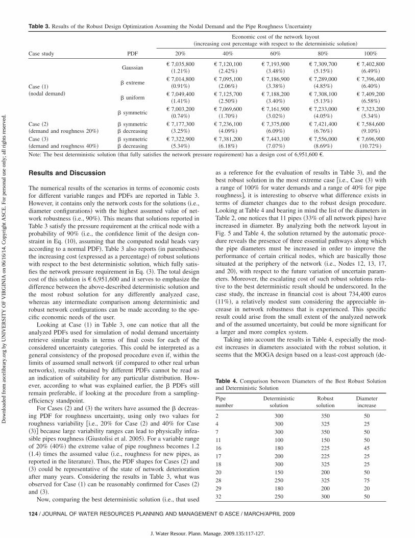
The case study is conceived in order to verify and demonstrate themethodology as applied to a real network. The featured system isthe distribution network of an Apulian town �Southern Italy�whose layout is depicted in Fig. 4 with the corresponding dataprovided in Table 1. Each pipe represented in Fig. 4 is listedaccording to its identification number �Pipe number�, and is ac-companied by its start and end nodes as well as its length �Li�. Allnodes are denoted by their identification number �Node number�and also appear in Table 1, which reports the relevant determin-istic demands �qj� �used as mean values for the uncertainty simu-lation� and elevations �Zi�. The node without an identificationnumber corresponds to the sole reservoir of the network, with thehead reported in Table 1 being the water level H01. Table 2 liststhe available pipe diameters, each coupled with its unit cost �ex-pressed in Euros per meter� and its deterministic unit resistancecoefficient,

Ri

Li= u =

�

Di5 =

8,57 � 10−4�1 +2�

Di

Di5 �13�

as evaluated by Bazin’s formula �Bazin and Darcy 1865; Manning1891�, using �=0.12. This coefficient is used as the mean value

Fig. 4. Apulian network layout

for uncertainty evaluation.



As explained earlier, the proposed procedure is conceived as ageneral one, with a certain number of parameters to be set. Re-ferring to Phase 1 �deterministic phase� the adopted minimumpressure head value �Pj

min� is equal to 10 m, whereas the range ofdefinition for the used second objective function �PDR� is �0;2�,thus admitting a lower pressure head limit of 8 m at the criticalnode. For Phase 2 �stochastic phase�, the assumed maximumnumber of samples to be taken �Smax� is 1,000, whereas the lowerlimit for samples �Smin� is equal to 30. This last choice derivesfrom the assumption that mean values and standard deviationsevaluated on, at least, 30 samples can be reasonably considered assufficiently statistically reliable �Benjamin and Cornell 1970�. Fi-nally, the assumed initial threshold for the number of samples�Sini� is equal to 100.

During Phase 2 optimization, as noted earlier, the evolvingPareto front can be bounded between two extreme values of net-work robustness. The assumed lower bound is 10% �the designconstraint in Eq. �10� is satisfied at the most critical node with aconfidence limit at least equal to 10%�, which implies that therelevant value for � is −1.282 �see Fig. 2�. The upper bound isimposed in order to confine robustness evaluation to what is tech-nically suitable, so the investigation assumes a maximum valueset to R=90%, corresponding to � equal to 1.282 �see Fig. 2�, asthe cost of solutions rises exponentially for robustness above90%, as noted by other authors �Kapelan et al. 2005; Tolson et al.2004�. During the MOGA run, networks exhibiting robustnessbeyond the assumed range are penalized. For example, a value ofR higher than 90% ��1.282� implies that the relevant networkis assumed to have a robustness of 90%, thus there is incentive toretain the design if it is cheaper; otherwise, when network robust-ness falls below 10% ��−1.282�, the solution is very cheap, butat the same time too low in robustness to be accepted �even lowerthan deterministic solution�.

As explained, the proposed approach consists of two phases:the deterministic least-cost design of the network and the robust/stochastic design that directly involves network robustness withinthe optimization. Both of these harness OPTIMOGA �Giustolisi etal. 2004� as an optimizer, using different additional objectivefunctions �minimization of pressure deficit at the critical node forPhase 1, maximization of network robustness for Phase 2�coupled with minimization of design costs. OPTIMOGA startswith a population made up of POPini individuals, POPini being setas 40 in this case. Each individual/chromosome is made up of anumber of genes that equals the number of network links in theproblem at stake, each gene being representative of the assumeddiameter for the network configuration. Genes are comprised be-tween 0 and 9, according to what is reported in Table 2. Thegenetic operators used are a multipoint crossover �with a prob-ability of 40%�, with a number of potential swapping points equalto the number of genes contained in the chromosomes. Care istaken in not swapping between two individuals’ genes represent-ing the same digit. A global mutation is initially used, each genecan be mutated with a 10% probability and assuming values rang-ing between 0 and 9. Afterwards, when the algorithm is in anexploitative phase of the Pareto front and it is not advisable toscatter the solutions in the objective space, a sort of local muta-tion is adopted, consisting in a small change of each mutatinggene �i.e., +1 or −1 with respect to its original value�. The selec-tion of the mating pool is pursued with respect to the size of thebest-found evolving Pareto front, by means of a rank-based fit-ness assignment �Fonseca and Fleming 1993�. Finally, runs can beended in two ways: by a stopping criterion based on the number
of generations achieved, or by a criterion based on the number of

ge. 2009.135:117-127.

Dow

nloa

ded

from

asc

elib

rary

.org

by

UN

IVE

RSI

TY

OF

VIR

GIN

IA o

n 06

/16/

14. C

opyr

ight

ASC

E. F

or p

erso

nal u

se o

nly;

all

righ

ts r

eser

ved.

solutions in the Pareto optimal set. In this case study the formerwas adopted, using 1,000 generations for the deterministic phaseand 200 generations for the stochastic phase. More details aboutOPTIMOGA features can be found in Giustolisi et al. �2004�.

Table 1. Apulian Network Data

Pipe

Pipenumber

Startnode

Endnode

Li

�m�

1 1 2 348

2 2 3 955

3 3 4 483

4 3 9 400

5 2 4 791

6 1 5 404

7 5 6 390

8 6 4 482

9 9 10 934

10 11 10 431

11 11 12 513

12 10 13 428

13 12 13 419

14 22 13 1,023

15 8 22 455

16 7 8 182

17 6 7 221

18 1 19 583

19 5 18 452

20 6 16 794

21 7 15 717

22 8 14 655

23 15 14 165

24 16 15 252

25 17 16 331

26 18 17 500

27 17 21 579

28 19 23 842

29 21 20 792

30 20 14 846

31 9 11 164

32 23 21 427

33 19 18 379

34 24 1 158

Table 2. Structural and Economic Features of Diameters into the ApulianNetwork

GAcoding

Nominaldiameter Ri /Li

Cost�€/m�

1 100 265.15 240.1

2 150 18.565 387.78

3 180 9.8824 435.66

4 200 5.6291 483.84

5 225 3.0681 542.34

6 250 1.6390 610.90

7 300 0.8668 690.24

8 325 0.4605 780.19

9 350 0.2466 881.55



The analyzed case study applies the above-described proce-dure to the robust design of the network assuming three uncer-tainty scenarios: �1� only the nodal demands are assumed to beuncertain; �2� and �3� both the nodal demands and roughness areconsidered uncertain, with different assumed pipe roughness un-certainty. In Case �1�, the � symmetric, � extreme, � uniform,and Gaussian PDF are used and compared. In Cases �2� and �3�,the only PDF considered for nodal demands is the � symmetricPDF, whereas the � decreasing PDF is employed for pipe rough-ness. The scenarios considered different values of variable rangerg �i.e., 20, 40, 60, 80, and 100% for nodal demands and 20 and40% for pipe roughness� with respect to the average assumedvalues for nodal demands and to the initial values for roughness�i.e., values for new pipe�, implying different bounded domainsfor the definition of any PDF. It is worth noting that some authors�Xu and Goulter 1999; Leonard et al. 2002; Tolson et al. 2004�have already used this kind of approach in order to simulate un-certainty in future demands and roughness. The ranges of thevariables employed in this paper are reasonably higher �demands�

Node

Nodenumber

qi

�L/s�Zi

�m�

1 10.863 6.4

2 17.034 7.0

3 14.947 6.0

4 14.280 8.4

5 10.133 7.4

6 15.350 9.0

7 9.114 9.1

8 10.510 9.5

9 12.182 8.4

10 14.579 10.5

11 9.0072 9.6

12 7.5745 11.7

13 15.200 12.3

14 13.550 10.6

15 9.226 10.1

16 11.200 9.5

17 11.469 10.2

18 10.818 9.6

19 14.675 9.1

20 13.318 13.9

21 14.631 11.1

22 12.012 11.4

23 10.326 10.0

Reservoir 0 H01=36.4

.5

.7

.0

.7

.9

.4

.6

.3

.4

.3

.1

.4

.0

.1

.1

.6

.3

.9

.0

.7

.7

.6

.5

.1

.5

.0

.9

.8

.6

.3

.0

.9

.2

.2

or comparable �roughness� with those reported in literature.


ge. 2009.135:117-127.

ssure r

Dow

nloa

ded

from

asc

elib

rary

.org

by

UN

IVE

RSI

TY

OF

VIR

GIN

IA o

n 06

/16/

14. C

opyr

ight

ASC

E. F

or p

erso

nal u

se o

nly;

all

righ

ts r

eser

ved.

Results and Discussion

The numerical results of the scenarios in terms of economic costsfor different variable ranges and PDFs are reported in Table 3.However, it contains only the network costs for the solutions �i.e.,diameter configurations� with the highest assumed value of net-work robustness �i.e., 90%�. This means that solutions reported inTable 3 satisfy the pressure requirement at the critical node with aprobability of 90% �i.e., the confidence limit of the design con-straint in Eq. �10�, assuming that the computed nodal heads varyaccording to a normal PDF�. Table 3 also reports �in parentheses�the increasing cost �expressed as a percentage� of robust solutionswith respect to the best deterministic solution, which fully satis-fies the network pressure requirement in Eq. �3�. The total designcost of this solution is € 6,951,600 and it serves to emphasize thedifference between the above-described deterministic solution andthe most robust solution for any differently analyzed case,whereas any intermediate comparison among deterministic androbust network configurations can be made according to the spe-cific economic needs of the user.

Looking at Case �1� in Table 3, one can notice that all theanalyzed PDFs used for simulation of nodal demand uncertaintyretrieve similar results in terms of final costs for each of theconsidered uncertainty categories. This could be interpreted as ageneral consistency of the proposed procedure even if, within thelimits of assumed small network �if compared to other real urbannetworks�, results obtained by different PDFs cannot be read asan indication of suitability for any particular distribution. How-ever, according to what was explained earlier, the � PDFs stillremain preferable, if looking at the procedure from a sampling-efficiency standpoint.

For Cases �2� and �3� the writers have assumed the � decreas-ing PDF for roughness uncertainty, using only two values forroughness variability �i.e., 20% for Case �2� and 40% for Case�3�� because large variability ranges can lead to physically infea-sible pipes roughness �Giustolisi et al. 2005�. For a variable rangeof 20% �40%� the extreme value of pipe roughness becomes 1.2�1.4� times the assumed value �i.e., roughness for new pipes, asreported in the literature�. Thus, the PDF shapes for Cases �2� and�3� could be representative of the state of network deteriorationafter many years. Considering the results in Table 3, what wasobserved for Case �1� can be reasonably confirmed for Cases �2�and �3�.

Table 3. Results of the Robust Design Optimization Assuming the Noda

Case study PDF

�in

20%

Case �1��nodal demand�

Gaussian€ 7,035,800

�1.21%�

� extreme€ 7,014,800

�0.91%�

� uniform€ 7,049,400

�1.41%�

� symmetric€ 7,003,200

�0.74%�

Case �2��demand and roughness 20%�

� symmetric� decreasing

€ 7,177,300�3.25%�

Case �3��demand and roughness 40%�

� symmetric� decreasing

€ 7,322,900�5.34%�

Note: The best deterministic solution �that fully satisfies the network pre

Now, comparing the best deterministic solution �i.e., that used



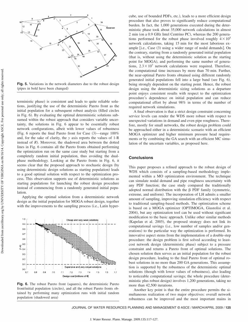
as a reference for the evaluation of results in Table 3�, and thebest robust solution in the most extreme case �i.e., Case �3� witha range of 100% for water demands and a range of 40% for piperoughness�, it is interesting to observe what difference exists interms of diameter changes due to the robust design procedure.Looking at Table 4 and bearing in mind the list of the diameters inTable 2, one notices that 11 pipes �33% of all network pipes� haveincreased in diameter. By analyzing both the network layout inFig. 5 and Table 4, the solution returned by the automatic proce-dure reveals the presence of three essential pathways along whichthe pipe diameters must be increased in order to improve theperformance of certain critical nodes, which are basically thosesituated at the periphery of the network �i.e., Nodes 12, 13, 17,and 20�, with respect to the future variation of uncertain param-eters. Moreover, the escalating cost of such robust solutions rela-tive to the best deterministic result should be underscored. In thecase study, the increase in financial cost is about 734,400 euros�11%�, a relatively modest sum considering the appreciable in-crease in network robustness that is experienced. This specificresult could arise from the small extent of the analyzed networkand of the assumed uncertainty, but could be more significant fora larger and more complex system.

Taking into account the results in Table 4, especially the mod-est increases in diameters associated with the robust solution, itseems that the MOGA design based on a least-cost approach �de-

and and the Pipe Roughness Uncertainty

Economic cost of the network layoutg cost percentage with respect to the deterministic solution�

40% 60% 80% 100%

7,120,100�2.42%�

€ 7,193,900�3.48%�

€ 7,309,700�5.15%�

€ 7,402,800�6.49%�

7,095,100�2.06%�

€ 7,186,900�3.38%�

€ 7,289,000�4.85%�

€ 7,396,400�6.40%�

7,125,700�2.50%�

€ 7,188,200�3.40%�

€ 7,308,100�5.13%�

€ 7,409,200�6.58%�

7,069,600�1.70%�

€ 7,161,900�3.02%�

€ 7,233,000�4.05%�

€ 7,323,200�5.34%�

7,236,100�4.09%�

€ 7,375,000�6.09%�

€ 7,421,400�6.76%�

€ 7,584,600�9.10%�

7,381,200�6.18%�

€ 7,443,100�7.07%�

€ 7,556,000�8.69%�

€ 7,696,900�10.72%�

equirement� has a design cost of 6,951,600 €.

Table 4. Comparison between Diameters of the Best Robust Solutionand Deterministic Solution

Pipenumber

Deterministicsolution

Robustsolution

Diameterincrease

2 300 350 50

4 300 325 25

7 300 350 50

11 100 150 50

16 180 225 45

17 200 225 25

18 300 325 25

20 150 200 50

28 250 325 75

29 180 200 20

32 250 300 50

l Dem

creasin

€

€

€

€

€

€


ge. 2009.135:117-127.

Dow

nloa

ded

from

asc

elib

rary

.org

by

UN

IVE

RSI

TY

OF

VIR

GIN

IA o

n 06

/16/

14. C

opyr

ight

ASC

E. F

or p

erso

nal u

se o

nly;

all

righ

ts r

eser

ved.

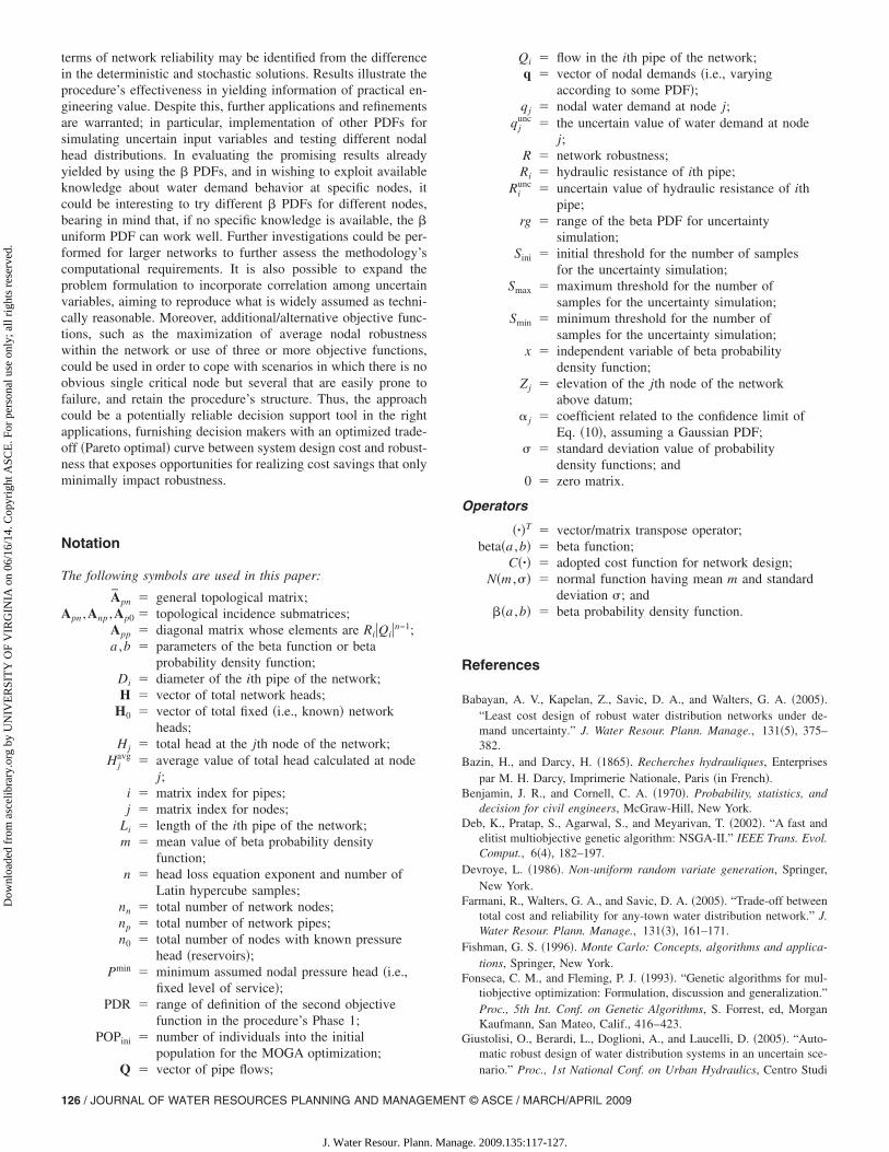
terministic phase� is consistent and leads to quite reliable solu-tions, justifying the use of the deterministic Pareto front as theinitial population for a subsequent robust analysis �filled circlesin Fig. 6�. By evaluating the optimal deterministic solutions sub-sumed within the robust approach that considers variable uncer-tainty, the solutions in Fig. 6 appear to be essentially robustnetwork configurations, albeit with lower values of robustness�Fig. 6 reports the final Pareto front for Case �3�—range 100%and, for the sake of clarity, the y axis reports the values of 1-Rinstead of R�. Moreover, the shadowed area between the dottedlines in Fig. 6 contains all the Pareto fronts obtained performingthe optimization run on the same case study but starting from acompletely random initial population, thus avoiding the dual-phase methodology. Looking at the Pareto fronts in Fig. 6, itseems clear that the proposed approach to stochastic design �byusing deterministic design solutions as starting population� leadsto a good optimal solution with respect to the optimization pro-cess. This observation supports use of deterministic solutions asstarting populations for launching the robust design procedureinstead of commencing from a randomly generated initial popu-lation.

Applying the optimal solution from a deterministic networkdesign as the initial population for MOGA robust design, togetherwith the improvements to the sampling process �i.e., Latin hyper-

Fig. 5. Variations in the network diameters due to the robust design�pipes in bold have been changed�

Fig. 6. The robust Pareto front �squares�, the deterministic Paretofront/initial population �circles�, and all the robust Pareto fronts ob-tained by performing many optimization runs with initial randompopulation �shadowed area�



cube, use of bounded PDFs, etc.�, leads to a more efficient designprocedure that also proves to significantly reduce computationalburden. In fact, the 1,000 generations executed during the deter-ministic phase took about 35,000 network calculations in almost2 min �on a 0.9 GHz Intel Centrino PC�, whereas the 200 genera-tions performed for the robust phase involved roughly 4�105

network calculations, taking 15 min for the most laborious ex-ample �i.e., Case �3� using a wider range of nodal demands�. Onthe contrary, starting from a randomly generated initial population�that is, without using the deterministic solution as the startingpoint for MOGA�, and performing the same number of genera-tions, 2.3�107 network calculations were required. Therefore,the computational time increases by more than 70 min. Further,the near-optimal Pareto fronts obtained using different randomlygenerated initial populations fell into a large band �see Fig. 6�,being strongly dependent on the starting point. Hence, the robustdesign using the deterministic sizing solutions as a departurepoint enjoys consistent results with respect to the optimizationprocedure’s dependence on initial population and can reducecomputational effort by about 98% in terms of the number ofrequired network simulations.

A final observation is that a strict design constraint concerningservice levels can render the WDS more robust with respect tounexpected variations in demand and even pipe roughness. There-fore, mostly for small networks, the robust design problem couldbe approached either in a deterministic scenario with an efficientMOGA optimizer and higher minimum pressure head require-ments or by combining the GA search with an efficient MC simu-lation of the uncertain variables, as proposed here.

Conclusions

This paper proposes a refined approach to the robust design ofWDS which consists of a sampling-based methodology imple-mented within a MO optimization environment. The techniquecan simulate nodal demand and pipe roughness uncertainty withany PDF function; the case study compared the traditionallyadopted normal distribution with the � PDF family �symmetric,extreme, and uniform�. The incorporation of LH admits a smalleramount of sampling, improving simulation efficiency with respectto traditional sampling-based methods. The optimization schemeis based on a MOGA optimizer �OPTIMOGA, Giustolisi et al.2004�, but any optimization tool can be used without significantmodification to the basic approach. Unlike other similar methods�Kapelan et al. 2005�, the proposed strategy does not link itscomputational savings �i.e., low number of samples and/or gen-erations� to the particular way the optimization is performed. Itsinnovative aspect stems from the implementation of a double-stepprocedure: the design problem is first solved according to least-cost network design �deterministic phase� subject to a pressureconstraint and returns a Pareto front of optimal solutions. Thechosen solution then serves as an initial population for the robustdesign procedure, leading to the final Pareto front of optimal ro-bust solutions in no more than 200 GA generations. This assump-tion is supported by the robustness of the deterministic optimalsolutions �though with lower values of robustness�, also leadingto noticeable computational savings; the whole procedure �deter-ministic plus robust design� involves 1,200 generations, taking nomore than 42,500 iterations.

Another key point is that the entire procedure permits the si-multaneous realization of two major objectives: overall network
robustness can be improved and the most important mains in

ge. 2009.135:117-127.

Dow

nloa

ded

from

asc

elib

rary

.org

by

UN

IVE

RSI

TY

OF

VIR

GIN

IA o

n 06

/16/

14. C

opyr

ight

ASC

E. F

or p

erso

nal u

se o

nly;

all

righ

ts r

eser

ved.

terms of network reliability may be identified from the differencein the deterministic and stochastic solutions. Results illustrate theprocedure’s effectiveness in yielding information of practical en-gineering value. Despite this, further applications and refinementsare warranted; in particular, implementation of other PDFs forsimulating uncertain input variables and testing different nodalhead distributions. In evaluating the promising results alreadyyielded by using the � PDFs, and in wishing to exploit availableknowledge about water demand behavior at specific nodes, itcould be interesting to try different � PDFs for different nodes,bearing in mind that, if no specific knowledge is available, the �uniform PDF can work well. Further investigations could be per-formed for larger networks to further assess the methodology’scomputational requirements. It is also possible to expand theproblem formulation to incorporate correlation among uncertainvariables, aiming to reproduce what is widely assumed as techni-cally reasonable. Moreover, additional/alternative objective func-tions, such as the maximization of average nodal robustnesswithin the network or use of three or more objective functions,could be used in order to cope with scenarios in which there is noobvious single critical node but several that are easily prone tofailure, and retain the procedure’s structure. Thus, the approachcould be a potentially reliable decision support tool in the rightapplications, furnishing decision makers with an optimized trade-off �Pareto optimal� curve between system design cost and robust-ness that exposes opportunities for realizing cost savings that onlyminimally impact robustness.

Notation

The following symbols are used in this paper:

Apn general topological matrix;Apn ,Anp ,Ap0 topological incidence submatrices;

App diagonal matrix whose elements are Ri�Qi�n−1;a ,b parameters of the beta function or beta

probability density function;Di diameter of the ith pipe of the network;H vector of total network heads;

H0 vector of total fixed �i.e., known� networkheads;

Hj total head at the jth node of the network;Hj

avg average value of total head calculated at nodej;

i matrix index for pipes;j matrix index for nodes;

Li length of the ith pipe of the network;m mean value of beta probability density

function;n head loss equation exponent and number of

Latin hypercube samples;nn total number of network nodes;np total number of network pipes;n0 total number of nodes with known pressure

head �reservoirs�;Pmin minimum assumed nodal pressure head �i.e.,

fixed level of service�;PDR range of definition of the second objective

function in the procedure’s Phase 1;POPini number of individuals into the initial

population for the MOGA optimization;
Q vector of pipe flows;


Qi flow in the ith pipe of the network;q vector of nodal demands �i.e., varying

according to some PDF�;qj nodal water demand at node j;

qjunc the uncertain value of water demand at node

j;R network robustness;Ri hydraulic resistance of ith pipe;

Riunc uncertain value of hydraulic resistance of ith

pipe;rg range of the beta PDF for uncertainty

simulation;Sini initial threshold for the number of samples

for the uncertainty simulation;Smax maximum threshold for the number of

samples for the uncertainty simulation;Smin minimum threshold for the number of

samples for the uncertainty simulation;x independent variable of beta probability

density function;Zj elevation of the jth node of the network

above datum;� j coefficient related to the confidence limit of

Eq. �10�, assuming a Gaussian PDF;� standard deviation value of probability

density functions; and0 zero matrix.

Operators

�·�T vector/matrix transpose operator;beta�a ,b� beta function;

C�·� adopted cost function for network design;N�m ,�� normal function having mean m and standard

deviation �; and��a ,b� beta probability density function.

References

Babayan, A. V., Kapelan, Z., Savic, D. A., and Walters, G. A. �2005�.“Least cost design of robust water distribution networks under de-mand uncertainty.” J. Water Resour. Plann. Manage., 131�5�, 375–382.

Bazin, H., and Darcy, H. �1865�. Recherches hydrauliques, Enterprisespar M. H. Darcy, Imprimerie Nationale, Paris �in French�.

Benjamin, J. R., and Cornell, C. A. �1970�. Probability, statistics, anddecision for civil engineers, McGraw-Hill, New York.

Deb, K., Pratap, S., Agarwal, S., and Meyarivan, T. �2002�. “A fast andelitist multiobjective genetic algorithm: NSGA-II.” IEEE Trans. Evol.Comput., 6�4�, 182–197.

Devroye, L. �1986�. Non-uniform random variate generation, Springer,New York.

Farmani, R., Walters, G. A., and Savic, D. A. �2005�. “Trade-off betweentotal cost and reliability for any-town water distribution network.” J.Water Resour. Plann. Manage., 131�3�, 161–171.

Fishman, G. S. �1996�. Monte Carlo: Concepts, algorithms and applica-tions, Springer, New York.

Fonseca, C. M., and Fleming, P. J. �1993�. “Genetic algorithms for mul-tiobjective optimization: Formulation, discussion and generalization.”Proc., 5th Int. Conf. on Genetic Algorithms, S. Forrest, ed, MorganKaufmann, San Mateo, Calif., 416–423.

Giustolisi, O., Berardi, L., Doglioni, A., and Laucelli, D. �2005�. “Auto-matic robust design of water distribution systems in an uncertain sce-
nario.” Proc., 1st National Conf. on Urban Hydraulics, Centro Studi

ge. 2009.135:117-127.

Dow

nloa

ded

from

asc

elib

rary

.org

by

UN

IVE

RSI

TY

OF

VIR

GIN

IA o

n 06

/16/

14. C

opyr

ight

ASC

E. F

or p

erso

nal u

se o

nly;

all

righ

ts r

eser

ved.

Drenaggio Urbano �CSDU�, Milano, Italy, 65–66 �Abstract Volumeand CD-ROM�.

Giustolisi, O., Doglioni, A., Savic, D. A., and Laucelli, D. �2004�. “Aproposal for an effective multi-objective non-dominated genetic algo-rithm: The optimised multi-objective genetic algorithm—OPTIMOGA.” Research Rep. No. 2004/07, School of Engineering,Computer Science and Mathematics, Centre for Water Systems, Univ.of Exeter, Exeter, U.K.

Giustolisi, O., Laucelli, D., and Savic, D. A. �2006�. “Development ofrehabilitation plans for water mains replacement considering risk andcost-benefit assessment.” Civ. Eng. Environ. Syst., 23�3�, 175–190.

Kapelan, Z. S., Savic, D. A., and Walters, G. A. �2005�. “Multiobjectivedesign of water distribution systems under uncertainty.” Water Resour.Res., 41�11�, W11407-1–W11407-15.

Lansey, K. E., Ning Duan Mays, L. W., and Yeou-Kung, T. �1989�.“Water distribution system design under uncertainties.” J. Water Re-sour. Plann. Manage., 115�5�, 630–645.

Leonard, M., Zecchin, A., Roberts, A., and Berrisford, M. �2002�. “Antcolony optimisation and risk-based assessment of water distributionsystems.” Final Year Research Project Rep., School of Civil and En-vironmental Engineering, Univ. of Adelaide, Adelaide, Australia.

Manning, R. �1891�. “On the flow of water in open channels and pipes.”Trans. Inst. Civ. Eng. Ireland, 20, 161–207.

McKay, M. D., Conover, W. J., and Beckman, R. J. �1979�. “A compari-



son of three methods for selecting values of input variables in theanalysis of output from a computer code.” Technometrics, 21�2�,239–245.

Mood, A. M., Graybill, F. A., and Boes, D. C. �1974�. Introduction to thetheory of statistics, McGraw-Hill, New York.

Savic, D. A. �2004�. “Risk and robust strategic investment planning in thewater industry, an optimisation approach.” Proc., 4th Int. Conf. onDecision Making in Urban and Civil Engineering �CD-ROM�, Uni-versity of Coimbra Press, Coimbra, Portugal.

Savic, D. A., and Walters, G. A. �1997�. “Genetic algorithms for theleast-cost design of water distribution networks.” J. Water Resour.Plann. Manage., 123�2�, 67–77.

Todini, E., and Pilati, S. �1988�. “A gradient algorithm for the analysis ofpipe networks.” Computer applications in water supply, Vol. 1, Wiley,London, 1–20.

Tolson, B. A., Maier, H. R., Simpson, A. R., and Lence, B. J. �2004�.“Genetic algorithms for reliability-based optimization of water distri-bution systems.” J. Water Resour. Plann. Manage., 130�1�, 63–72.

Walski, T. M. �2001�. “The wrong paradigm—Why water distributiondoesn’t work?” J. Water Resour. Plann. Manage., 127�4�, 203–205.

Xu, C., and Goulter, I. C. �1999�. “Reliability-based optimal design ofwater distribution network.” J. Water Resour. Plann. Manage.,125�6�, 352–362.


ge. 2009.135:117-127.

Documents

Deterministic versus Stochastic Design of Water Distribution Networks