DETERMINATION OF PHASE{SPACE RECONSTRUCTION … · Determination of Phase{Space Reconstruction Parameters 561 The reconstruction results are the same as those given by Kim et al

KYBERNET IK A — VOLUME 4 4 ( 2 0 0 8 ) , NU MB ER 4 , P AG E S 5 5 7 – 5 7 0

DETERMINATION OF PHASE–SPACERECONSTRUCTION PARAMETERSOF CHAOTIC TIME SERIES

Wei-Dong Cai, Yi-Qing Qin and Bing-Ru Yang

A new method called C–C–1 method is suggested, which can improve some drawbacksof the original C–C method. Based on the theory of period N , a new quantity S(t) forestimating the delay time window of a chaotic time series is given via direct computing atime-series quantity S(m, N, r, t), from which the delay time window can be found. Theoptimal delay time window is taken as the first period of the chaotic time series with alocal minimum of S(t). Only the first local minimum of the average of a quantity ∆S2(t) isneeded to ascertain the optimal delay time. The parameter of the C–C method – embeddingdimension m – is adjusted rationally. In the new method, the estimates of the optimal delaytime and the optimal delay time window are more appropriate. The robustness of the C–C–1 method reaches 40%, whereas that of the C–C method is 30%.

Keywords: phase-space reconstruction, embedding window, delay time, time series

AMS Subject Classification: 37D45

1. INTRODUCTION

Strange attractors embody the characteristics of chaotic systems. The evolvementof any component in a chaotic system is determined by other components whichinteracting each other, therefore the information of these correlated components isunderlying in the evolution process of the component [2]. Analyses to chaotic timeseries are mostly based on the phase-space reconstruction. In [8, 10], Packard et al.suggested that the phase-space can be restructured from observing the single delaycoordinate of the dynamical system, and the fundamental theorem of reconstruction,introduced by Takens [10, 11] and extended more recently in [9], gives no restrictionon the time delay constant τ while for m states a sufficient (but not necessary)condition is m ≥ 2d+1, where d is the fractal dimension of the underlying attractor,and m is the phase-space dimension. The theorem of phase-space reconstruction isas follows:

The method of delays can be used to embed a scalar time series {x(ti),i = 1, 2, . . . , N} into an m-dimensional space X(ti) = (x(ti), x(ti + τ), . . . ,x(ti +(m−1)τ)), i = 1, 2, . . . ,M , where τ is the delay time, m is the embedding

558 W.D. CAI, Y.Q. QIN AND B.R. YANG

dimension, M is the number of embedded points in the m-dimensional space, andM = N − (m − 1)τ . Set {X(ti), i = 1, 2, . . . ,M} shows the tracks of the strangeattractor in the phase-space, and the chaotic evolvement of the dynamical systemcan be studied in the reconstructed m-dimensional space. Research shows that thereconstructed phase-space with appropriate m and τ has the same quality of diffeo-morphism as the original dynamical system.

The selections of m and τ are rather important but difficult in the phase-spacereconstruction [7]. There are two main points of selecting m and τ , see e. g. [5, 12,13, 14].

Point 1: The selections of m are independent of the selections of τ . The selectionsof m and τ are based on 3 rules. The first one is the method of serial correlation,such as autocorrelation function, mutual information, high-order correlation, and soon; the second one is the method based on phase-space expansion, such as fill factor,average displacement, SVF, and so on; the last one includes the method of multi-ple autocorrelation function and the method of non-biased multiple autocorrelationfunction.

Point 2: m and τ are correlated one another for the reason that real data setsare finite and noisy. Tests show that the delay time window is τw = (m− 1)τd, andit is the entire time spanned by the components of {X(ti)}, which is independent ofm instead. In this case, the delay time τd varies with the embedding dimension m.τw is comparatively steady for a certain time series, and the irrelevant partnershipof m will affect the equivalence relationship between the reconstructed phase-spaceand the former space. Thus, some combined computing methods come into being,such as the C-C method [3], the time window length, the automated embedding andthe creep phenomenon, and so on.

Many researchers agree with Point 2 above. They consider that the process ofmutual information is rather cumbersome computationally, whereas the autocorre-lation function only treats the linear dependence of the time series and it does nottreat the nonlinearity appropriately, but it may yield an incorrect value for the delaytime τd. The C–C method suggested is most popular, which gives the delay timeτd and delay time window τw simultaneously by applying the correlation integral.Based on the statistical results, although the C–C method lacks theoretical support,it runs well in practice and it shows some advantages, such as simple operation,lower algorithm complexity, reliability for less data and better robustness, etc. Ithas become a regular method for analyzing the time series [4].

Aiming at improving some drawbacks of the C–C method, this paper suggestsan advanced method to determine the optimal delay time τd and the optimal delaytime window τw. It improves the computing process, parameter selections and thedetermination rules of the C–C method. The selections of the optimal delay timewindow τw are more reliable and stable, the determination of the optimal delay timeτd is more appropriate, and the robustness is higher than that of the C–C method.

Determination of Phase–Space Reconstruction Parameters 559

2. ANALYSIS OF THE C–C METHOD

2.1. Algorithm of the C–C method

Let the chaotic time series be x = {xi, i = 1, 2, . . . , N}, where m is the embeddingdimension, τd is the delay time, and denote X = {Xi}, where Xi are the points inthe m-dimensional space:

Xi = (xi, xi + τ, . . . , xi + (m− 1)τ)T , i = 1, 2, . . . ,M. (1)

Thus, the correlation integral for the embedded time series is [1]:

C(m,N, r, t) =2

M(M − 1)

∑

1≤i<j≤M

θ(r − dij), r > 0 (2)

where m is the embedding dimension, N is the data number of the time series, r isthe search radius, t is the delay time, M = N − (m− 1)t is the number of embeddedpoints in the m-dimensional space, θ(x) is the Heaviside function: θ(x) = 0, if x <0; θ(x) = 1, if x ≥ 0, and dij =‖ xj − xj ‖∞ denotes the sup-norm.

Correlation integral is a cumulative distribution function, which denotes the prob-ability of distances between any pairs of points in the phase-space that are not greaterthan r. The distance between a pair of points is denoted by the sup-norm of thedifference between the two vectors. Define the statistical quantity of the time seriesby

S(m,N, r, t) = C(m,N, r, t)− Cm(1, N, r, t). (3)

The computing process of Eq. (3) is to subdivide the time series x = {xi} into tdisjoint time series averagely, where t is the reconstructive delay time, i. e.

x(1) = {x1, xt+1, . . . , xbN/tc−t+1}x(2) = {x2, xt+2, . . . , xbN/tc−t+2}. . .x(t) = {xt, xt+t, . . . , xbN/tc}.

(4)

Here, define the average of the statistical quantity given by Eq. (3) as follows:

S1(m,N, r, t) =1t

t∑

s=1

[Cs(m, N, r, t)− Cms (1, N, r, t)]. (5)

As N →∞ , we can write

S1(m, r, t) =1t

t∑

s=1

[Cs(m, r, t)− Cms (1, r, t)]. (6)

For fixed m and t, S1(m, r, t) is identically equal to 0 for all r if x = {xi} isindependently and identically distributed (i.i.d.) and N → ∞. However, real datasets are finite, and the data may be correlated with noise; so, in general, S1(m, r, t) 6=


0. Thus, the locally optimal times may be either the zero crossings of S1(m, r, t) orthe times at which S1(m, r, t) shows the least variation in r, since this indicates anearly uniform distribution of points. Hence, we select several representative valuesrj , and define the quantity

∆S1(m, t) = max{S1(m, ri, t)} −min{S1(m, ri, t)} (7)

which is a measure of the variation of S1(m, r, t) in r. The locally optimal times tare then the zero crossings of S1(m, r, t) ∼ t and the minima of ∆S1(m, t) ∼ t. Thezero crossings of S1(m, r, t) ∼ t should be nearly the same for all m and r, and theminima of S1(m, r, t) ∼ t should be nearly the same for all m (otherwise, the time isnot locally optimal). The delay time τd will correspond to the first of these locallyoptimal times.

Appropriate choices for m, N and r may be found by examining the BDS statis-tic. Generally, for N = 3000, m = 2, 3, 4, 5, t = 1, 2, . . . , 200, r = k × σ/2,k = 1, 2, 3, 4, where σ = std (x) is the standard deviation of the time series. Wethen define the following averages of the quantities given by Eqs. (6) and (7):

S1(t) =116

4∑

m=1

4∑

i=1

S1(m, ri, t) (8)

∆S̄1(t) =14

4∑

m=1

∆S1(m, t) (9)

and we look for the first zero crossing of S1(t) or the first local minimum of ∆S̄1(t)to find the first locally optimal time for independence of the data, which gives thedelay time τd. The optimal time is the delay time t for which S̄1(t) and ∆S̄1(t) areboth closest to 0. If we assign equal importance to these two quantities, then wemay simply look for the minimum of the quantity

S1 cor(t) = ∆S̄1(t)+ | S̄1(t) | (10)

and this optimal time gives the delay time window τw.

2.2. Numerical examples of the C–C method

In these examples, we observe variable x from the chaotic Lorenz system by inte-grating equations using function ode45 in MATLAB. The Lorenz system (11) is asfollows:

dx/dt = −σx + σy

dy/dt = −xz + rx− y

dz/dt = xy − bz

(11)

where σ, r and b are constants. We solve this system of equations for [σ, r, b] =[16.0, 4.0, 45.92], with initial conditions [x, y, z] = [−1, 0, 1], to generate a time seriesof the variable x with interval of integration from 0 to 1000, step h = 0.01.


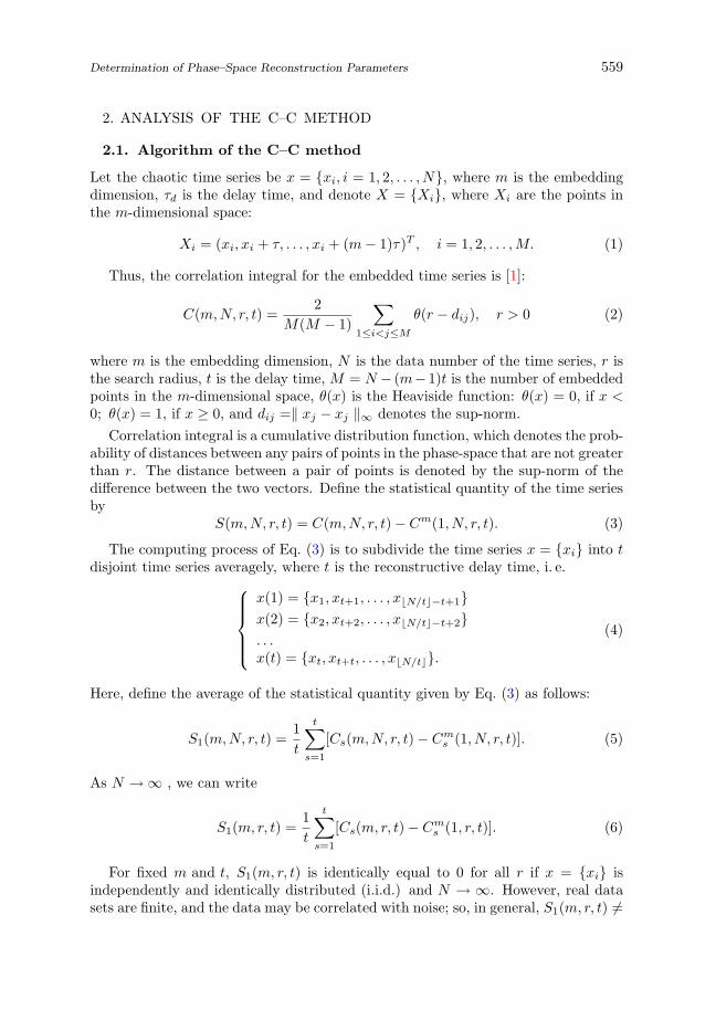
The reconstruction results are the same as those given by Kim et al. in [3], testedby 3000 points selected from 53001 to 56000 (Figure 1).

0 20 40 60 80 100 120 140 160 180 200-0.1

0

0.1

0.2

0.3

0 20 40 60 80 100 120 140 160 180 2000

0.1

0.2

0.3

0.4

10t =

1_ (100) 0.01corS =

1

1

1_

( )

∆ ( )

( )

cor

S t

S t

t

S t

t

−

•

−

Fig. 1. C–C method: analysis on variable x from the Lorenz system.

2.3. Drawbacks of the C–C method

While the numerical examples are carrying on, we also select 3000 points from dif-ferent intervals to estimate the optimal delay time τd and the optimal delay timewindow τw. The results are shown in Table 1.

Table 1. C–C method: results of the reconstructed

variable x from the Lorenz system.

Sample Interval m τd τw

10001–13000 21 10 19120001–23000 15 10 13230001–33000 20 10 18440001–43000 11 11 10450001–53000 14 11 13760001–63000 14 11 13770001–73000 9 11 8480001–83000 17 10 15290001–93000 11 11 101

There are at least 3 drawbacks in the C–C method.


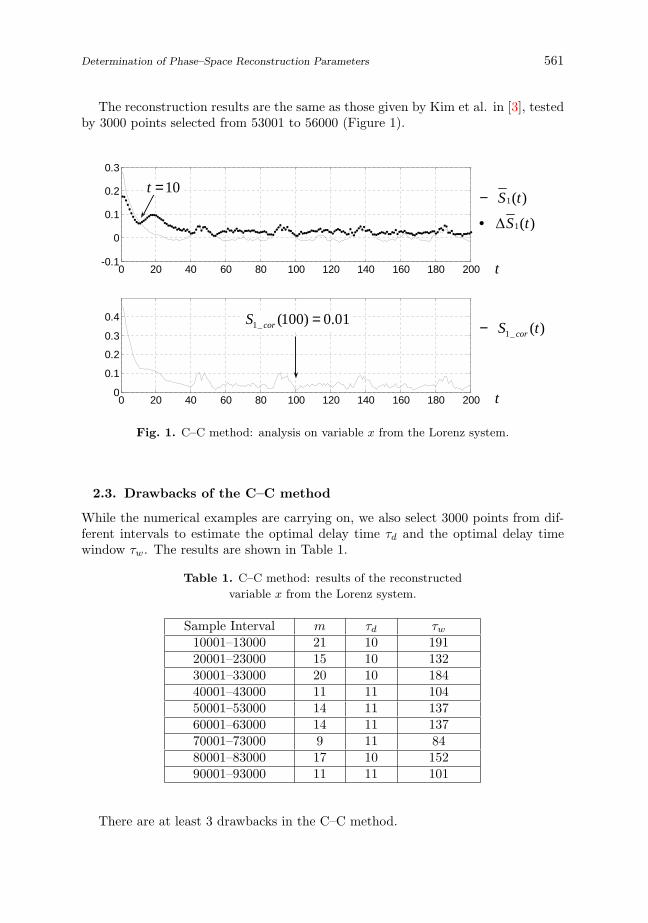
(1) Ideally the minimum of S1 cor(t) is the optimal delay time window τw, whereasin the tests there are some local minimal points whose values are much closeto the minimum of S1 cor(t). They disturb the estimate of the minimum ofS1 cor(t). And even worse, the optimal delay time window τw is not the exactminimum point, which may mislead the estimate of the optimal delay timewindow τw. In Figure 2, the marked points are all likely to be the optimaldelay time window τw.

40 60 80 100 120 140 160 180 2000

0.02

0.04

0.06

0.08

0.1

1_ ( )

corS t

t

−

Fig. 2. C–C method: results of the local minima and the minimum of S1 cor(t).

(2) In practice, the first zero crossing of S1(t) is unequal to the first local minimumof ∆S1(t). But for the time series with period T , for t = kT, k = 1, 2, . . ., oneof the points is mostly not only the first zero crossing of S̄1(t) but also theminimum of S1 cor(t); therefore, paradoxical conclusions can be drawn. Wesuggest that it is not appropriate to take the first zero crossing of S̄1(t) asthe optimal delay time τd. We may consider taking the first local minimum of∆S̄1(t) as the first locally optimal time τw.

(3) Strictly speaking, a chaotic system has no period. For low-dimensional chaoticsystems with period N , the mean orbital period T is the mean period gen-erated by the oscillations of the chaotic attractor in the phase-space orbits.The computing mode of Eq. (5) leads to the following result: if t = kT, k =1, 2, . . . , then ∆S̄1(t) = 0, and ∆S̄1(t) shows high-frequency oscillations in-creasingly along with the increase of t. When the value of the optimal delaytime τd is big enough, the high-frequency oscillations can even affect the esti-mate of the first local minimum of ∆S̄1(t).

Aiming at improving the drawbacks of the C–C method, we suggest an improvedmethod of phase-space reconstruction, which is called C–C–1 method.


3. THE IMPROVED METHOD: C–C–1 METHOD

3.1. Algorithm of the C–C–1 method

By comparing S(m,N, r, t) with S1(m,N, r, t) in Eq. (5), for fixed m, and n →∞,S1(m,N, r, t) ∼ t shows high-frequency oscillations increasingly along with the in-crease of t. In Eq. (3), on the same conditions, generally S(m,N, r, t) ∼ t has thesame oscillations characteristics as S1(m,N, r, t) ∼ t, whereas the high-frequencyoscillations of S1(m,N, r, t) ∼ t disappear.

Therefore, instead of subdividing the time series x = {xi} into t disjoint timeseries, the C–C–1 method computes S(m, N, r, t) directly. Since chaotic time serieshas intrinsic determinacy, and the direct algorithm is rather cumbersome computa-tionally, in order to reduce the time complexity, the statistical quantity S(m,N, r, t)given by Eq. (3) is computed with another average method. Being different from theC–C method, a positive integer p is selected as a constant, which is independent ofthe delay time t, to subdivide the reconstructed phase-space X = {X(ti)}; and ac-cording to the calculation of S1(t) and ∆S̄1(t) in the C–C method, S̄2(t) and ∆S̄2(t)are calculated.

Numbers of tests show that S2 cor(t) have some clear peak values with qualita-tively chaotic period N , and all of the points that bring these clear peak values arethe local minima of S1 cor(t). Thus, a new determinative rule of the optimal delaytime window τw is given: to estimate the optimal delay time window τw, the C–Cmethod looks for the minimum of S1 cor(t), whereas the C–C–1 method combines theclear peak values of S2 cor(t) with the chaotic period N and with the local minimaof S1 cor(t). By looking for the first local minimum peak value of S1 cor(t)−S2 cor(t)with the clear quality of chaotic period N , we estimate the optimal delay time win-dow τw; and aiming at the results with no clear quality of chaotic period N , we selectthe minimum of S1 cor(t)− S2 cor(t) to estimate the optimal delay time window τw.

Furthermore, the C–C method looks for the first zero crossing of S̄1(t) or thefirst local minimum of ∆S1(t) as the first optimal delay time τd, while the C–C–1method just looks for the first local minimum of ∆S̄2(t) as the first optimal delaytime τd.

The algorithm of the C–C–1 method is summarized as follows:

The phase-space reconstruction is the first step. Then, a positive integer p isselected as a constant, which is independent of the delay time t, to subdivide thereconstructed phase-space X = {X(ti)}:

X(1) = {X1, Xp+1, . . . , XbN/pc−p+1}X(2) = {X2, Xp+2, . . . , XbN/pc−p+2}. . .X(p) = {Xp, Xp+p, . . . , XbN/pc}

(12)


x(1) = {X1(1), X1(2), . . . , X1(m), Xp+1(1), Xp+1(2), . . . , Xp+1(m), . . .}x(2) = {X2(1), X2(2), . . . , X2(m), Xp+2(1), Xp+2(2), . . . , Xp+2(m), . . .}. . .x(p) = {Xp(1), Xp(2), . . . , Xp(m), Xp+p(1), Xp+p(2), . . . , Xp+p(m), . . .}.

(13)

We define the average of the statistical quantity given by Eq. (3) as follows:

S2(m, r, t) =1p

p∑

s=1

Cs(m, r, t)−[1pCs(1, r, t)

]m

(14)

where p is an adjustable parameter to balance the precision and speed of calculation.The definitions of ∆S2(m, t), S̄2(t), ∆S̄2(t) and S2 cor(t) are all the same as Eqs. (7),(8), (9) and (10).

For p = 1, Eq. (14) is equal to Eq. (3), so the results of S2(m, r, t) have thehighest precision, but the algorithm has the highest time complexity. For p > 1,the algorithm has the lower time complexity. Tests show that although the newalgorithm still has a few errors (the same situation as that in the C–C method),these errors do not disturb the estimates of the local minima.

Furthermore, we just look for the first local minimum of ∆S̄2(t) as the firstoptimal delay time τd. Considering S1 cor(t) and S2 cor(t) roundly, if we assign equalimportance to these two quantities, and define a new quantity

Scor(t) = S1 cor(t)− S2 cor(t) (15)then we may simply look for the first local minimum peak value of the quantityScor(t) with the clear quality of chaotic period N . This optimal time gives theoptimal delay time window τw; but if the results are not with clear quality of chaoticperiod N , the minimum of Scor(t) gives the optimal delay time window τw.

3.2. Numerical examples of the C–C–1 method

As tests, we apply the C–C–1 method to the Lorenz system. Large numbers ofsimulations prove that the adjustments to the ranges of the embedding dimension mcan help to obtain a more appropriate optimal delay time τd. Let m = 2, 3, . . . , 7, p =60, and other conditions be the same as the C–C method.

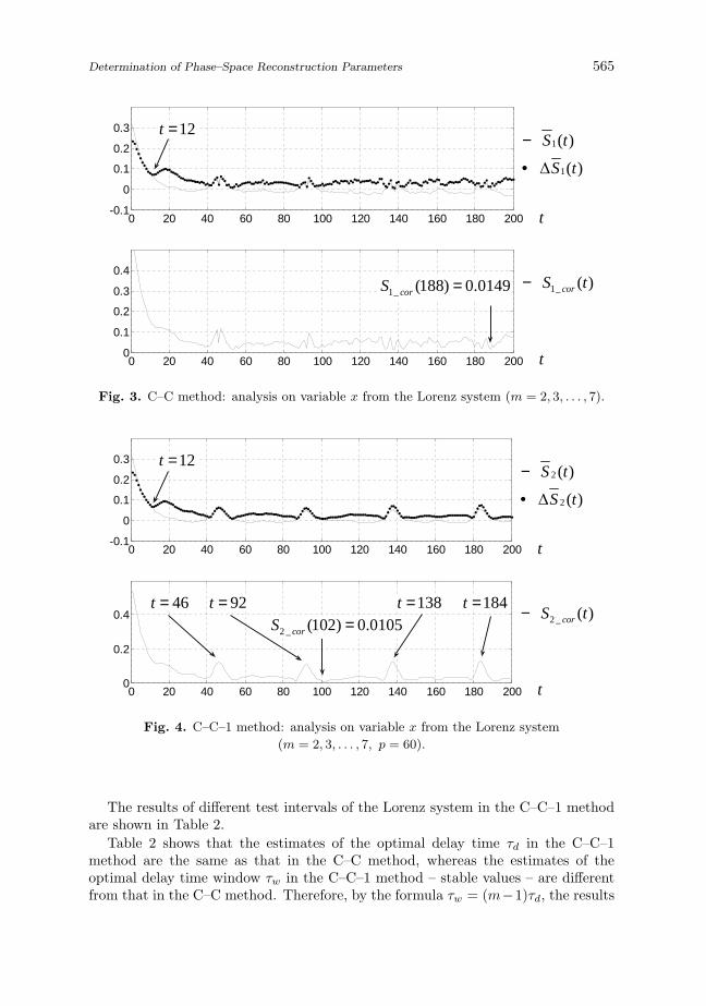
Figures 3, 4, and 5 show some contrastive results between the C–C method andthe C–C–1 method (where 3000 points are selected from 60001 to 63000).

Analyzing Figures 3, 4, and 5 shows that high-frequency oscillations are stillincreasing along with the increase of t but they are improved significently, and moreimportantly, the local maxima with the chaotic period N can be found from thegraph of the phase-space reconstruction (Figure 4).

In Figure 4, when t = 46, 92, 138, 184, the clear maximum peak values of S2 cor(t)with the quality of chaotic period N are given. Comparing with Figure 3, thesevalues are all local minima of S1 cor(t). Thus, an important conclusion is drawn: inthe C–C–1 method, the optimal delay time window τw is estimated by the first localminimum peak value of Scor(t), with a clear quality of chaotic period N .


0 20 40 60 80 100 120 140 160 180 200-0.1

0

0.1

0.2

0.3

0 20 40 60 80 100 120 140 160 180 2000

0.1

0.2

0.3

0.4

12t =

1_ (188) 0.0149corS =

1

1

1_

( )

∆ ( )

( )

cor

S t

S t

t

S t

t

−

•

−

Fig. 3. C–C method: analysis on variable x from the Lorenz system (m = 2, 3, . . . , 7).

0 20 40 60 80 100 120 140 160 180 200-0.1

0

0.1

0.2

0.3

0 20 40 60 80 100 120 140 160 180 2000

0.2

0.4

12t =

2 _ (102) 0.0105corS =

2

2

2 _

( )

∆ ( )

( )

cor

S t

S t

t

S t

t

−

•

−46t = 92t = 138t = 184t =

Fig. 4. C–C–1 method: analysis on variable x from the Lorenz system

(m = 2, 3, . . . , 7, p = 60).

The results of different test intervals of the Lorenz system in the C–C–1 methodare shown in Table 2.

Table 2 shows that the estimates of the optimal delay time τd in the C–C–1method are the same as that in the C–C method, whereas the estimates of theoptimal delay time window τw in the C–C–1 method – stable values – are differentfrom that in the C–C method. Therefore, by the formula τw = (m−1)τd, the results


0 20 40 60 80 100 120 140 160 180 200-0.15

-0.1

-0.05

0

0.05

0.1

( )

corS t

t

−

46t = 92t = 138t = 184t =

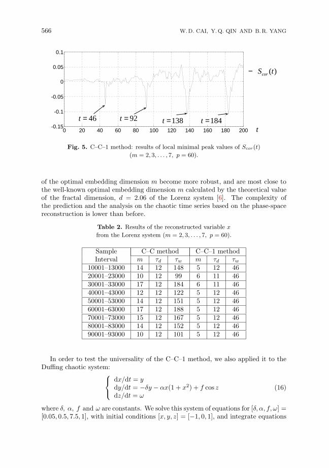
Fig. 5. C–C–1 method: results of local minimal peak values of Scor(t)

(m = 2, 3, . . . , 7, p = 60).

of the optimal embedding dimension m become more robust, and are most close tothe well-known optimal embedding dimension m calculated by the theoretical valueof the fractal dimension, d = 2.06 of the Lorenz system [6]. The complexity ofthe prediction and the analysis on the chaotic time series based on the phase-spacereconstruction is lower than before.

Table 2. Results of the reconstructed variable x

from the Lorenz system (m = 2, 3, . . . , 7, p = 60).

Sample C–C method C–C–1 methodInterval m τd τw m τd τw

10001–13000 14 12 148 5 12 4620001–23000 10 12 99 6 11 4630001–33000 17 12 184 6 11 4640001–43000 12 12 122 5 12 4650001–53000 14 12 151 5 12 4660001–63000 17 12 188 5 12 4670001–73000 15 12 167 5 12 4680001–83000 14 12 152 5 12 4690001–93000 10 12 101 5 12 46

In order to test the universality of the C–C–1 method, we also applied it to theDuffing chaotic system:

dx/dt = ydy/dt = −δy − αx(1 + x2) + f cos zdz/dt = ω

(16)

where δ, α, f and ω are constants. We solve this system of equations for [δ, α, f, ω] =[0.05, 0.5, 7.5, 1], with initial conditions [x, y, z] = [−1, 0, 1], and integrate equations


by function ode45 in MATLAB, to generate a time series of the variable x withinterval of integration from 0 to 5000, step h = 0.05.

In testing the Duffing system, we select 3000 points from 50001 to 53000. Form = 2, 3, . . . , 7, p = 60, and in order to show the characteristic of the chaotic periodN , we let t = 1, 2, . . . , 300.

The reconstructed results of x from the Duffing system in the C–C method andthe C–C–1 method are shown in Figures 6, 7, and 8. The local minimum peakvalues with the chaotic period N are also given in the graph of the phase-spacereconstruction.

0 50 100 150 200 250 300-0.1

0

0.1

0.2

0.3

0 50 100 150 200 250 3000

0.2

0.4

14t =

1_ (161) 0.0626corS =

1

1

1_

( )

∆ ( )

( )

cor

S t

S t

t

S t

t

−

•

−1_ (251) 0corS =

Fig. 6. C–C method: analysis on variable x from the Duffing system (m = 2, 3, . . . , 7).

Analyses show that the C–C–1 method has broader universality and a more appro-priate optimal delay time window τw, and the optimal delay time τd can be obtained.

4. NOISE EFFECTS

To study the effects of noise on the C–C–1 method, we add Gaussian noise to theLorenz time series. Specifically, we examine the time series yi = xi + ησεi, where xi

is the noise-free Lorenz time series, σ is its standard deviation, εi is a Gaussian i.i.d.random variable with zero mean and a standard deviation of 1, and η is the strengthof the noise. Noise levels of 10%, 20%, . . . , and 60% (with η = 0.1, 0.2, . . . , 0.6)are added to the Lorenz time series, and the C–C–1 method is performed for eachof these noise levels. According to the error standard given in [3], we observe thatthe estimates of the optimal delay time τd and the optimal delay time window τw

remain unchanged for η = 0.1, 0.2, 0.3, 0.4, but not for η = 0.5, 0.6. The results showthat the robustness of the C–C–1 method reaches 40%, whereas that of the C–Cmethod is 30%.


0 50 100 150 200 250 3000

0.1

0.2

0.3

0.4

0 50 100 150 200 250 3000

0.2

0.4

14t =

2 _ (79) 0.0896corS =

2

2

2 _

( )

∆ ( )

( )

cor

S t

S t

t

S t

t

−

•

−126t = 251t =

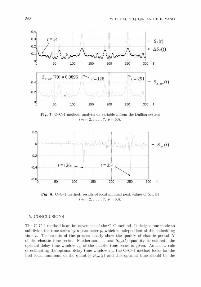
Fig. 7. C–C–1 method: analysis on variable x from the Duffing system

(m = 2, 3, . . . , 7, p = 60).

0 50 100 150 200 250 300-0.6

-0.4

-0.2

0

0.2

( )

corS t

t

−

126t = 251t =

Fig. 8. C–C–1 method: results of local minimal peak values of Scor(t)

(m = 2, 3, . . . , 7, p = 60).

5. CONCLUSIONS

The C–C–1 method is an improvement of the C–C method. It designs one mode tosubdivide the time series by a parameter p, which is independent of the embeddingtime t. The results of the process clearly show the quality of chaotic period Nof the chaotic time series. Furthermore, a new Scor(t) quantity to estimate theoptimal delay time window τw of the chaotic time series is given. As a new ruleof estimating the optimal delay time window τw, the C–C–1 method looks for thefirst local minimum of the quantity Scor(t) and this optimal time should be the


first period of the chaotic time series. On the other hand, we point out that inthe C–C method the rule of determining the optimal delay time τd by choosing thezero crossings of S̄1(t) may lead to an incorrect value. The C–C–1 method looks forthe first local minimum of ∆S̄2(t), which gives the optimal delay time τd. In thecomputing process, the parameter of the C–C method – embedding dimension m –is adjusted rationally in order to obtain more appropriate estimates of the optimaldelay time τd. Tests show that the C–C–1 method can give more reliable and stableestimates of the optimal delay time window τw and the optimal delay time τd. Wealso demonstrate the robustness of this method in the presence of noise. The noiselevels reach 40%, which is about 10% higher than that of the C–C method.

ACKNOWLEDGEMENT

This research was partially supported by the National Nature Science Foundation of China(grant No. 60675030), the Science and Technology Project of Education Office of ShandongProvince of China (project No. J06G01), and the Science and Research Foundation Projectof University of Ji’nan of China (project No.Y0614).

(Received September 30, 2007.)

REFERENC ES

[1] P. Grassberger and I. Procaccia: Measure the strangeness of strange attractors. Phys-ica D 9 (1983), 189–208.

[2] R. S. Huang: Chaos and Application. Wuhan University Press, Wuhan 2000.[3] H. S. Kim, R. Eykholt, and J.D. Salas: Nonlinear dynamics, delay times, and embed-

ding windows. Physica D 127 (1999), 48–60.[4] J. H. Lu, J.A. Lu, and S. H. Chen: Analysis and Application of Chaotic Time Series.

Wuhan University Press, Wuhan 2002.[5] X.Q. Lu, B.Cao, and M. Zeng et al. An algorithm of selecting delay time in the mutual

information method. Chinese J. Comput. Physics 23 (2006), 184–188.[6] H.G. Ma, X. H. Li, and G.H. Wang: Selection of embedding dimension and delay time

in phase space reconstruction. J. Xi’an Jiaotong University 38 (2004), 335–338.[7] M. Small and C. K. Tse: Optimal embedding parameters: A modeling paradigm.

Physica D: Nonlinear Phenomena 194 (2004), 283–296.[8] N.H. Packard, J. P. Crutchfield, J.D. Farmer et al. Geometry from a time series. Phys.

Rev. Lett. 45 (1980), 712–716.[9] T. Sauer, J. A. Yorke, and M. Casdagli: Embedology. J. Statist. Phys. 65 (1991),

579–616.[10] F. Takens: Detecting Strange Attractors in Turbulence. Dynamical Systems and Tur-

bulence. (Lecture Notes in Mathematics 898.) Springer-Verlag, Berlin 1981, pp. 366–381.

[11] F. Takens: On the Numerical Determination of the Dimension of an Attractor. Dynam-ical System and Turbulence. (Lecture Notes in Mathematics 1125.) Springer-Verlag,Berlin 1985, pp. 99–106.

[12] Y. Wang and W. Xu: The methods and performance of phase space reconstructionfor the time series in Lorenz system. J. Vibration Engrg. 19 (2006), 277–282.

[13] C.B. Xiu, X.D. Liu, and Y.H. Zhang: Selection of embedding dimension and delaytime in the phase space reconstruction. Trans. Beijing Institute of Technology 23(2003), 219–224.


[14] Y. Zhang and C. L. Ren: The methods to confirm the dimension of re-constructedphase space. J. National University of Defense Technology 27 (2005), 101–105.

Wei-Dong Cai, School of Information Science and Engineering, University of Ji’nan,

Ji’nan 250022 and School of Information Engineering, University of Science and Tech-

nology Beijing, Beijing 100083. China.

e-mail: [email protected]

Yi-Qing Qin, Computer School, Beijing Information Science & Technology University,

Beijing 100085, China and School of Information Engineering, University of Science

and Technology Beijing, Beijing 100083. China.

e-mail: qyq [email protected]

Bing-Ru Yang, School of Information Engineering, University of Science and Technology

Beijing, Beijing 100083. China.

e-mail: bryang [email protected]

Documents

DETERMINATION OF PHASE{SPACE RECONSTRUCTION … · Determination of Phase{Space Reconstruction Parameters 561 The reconstruction results are the same as those given by Kim et al