DETERMINATION OF LONG TERM DISTRIBUTION OF PETROBRAS ... · PETROBRAS/CENPES Edison C. P. de Lima, Luis V. S. Sagrilo and Gilberto B. Ellwanger COPPE/UFRJ Abstract — The tension

DETERMINATION OF LONG TERM DISTRIBUTION OF

STRESS RANGES FOR FATIGUE RELIABILITY

ANALYSIS OF A TLP DESIGNED FOR CAMPOS BASIN

Carlos Alberto BardanachviliPETROBRAS/CENPESEdison C. P. de Lima, Luis V. S. Sagrilo and Gilberto B. EllwangerCOPPE/UFRJ

Abstract — The tension leg platform (TLP) is a type of structural system forexploitation of oil and gas fields below sea floor and must be designed to avoidfatigue damage due to cyclic action of sea waves. Fatigue is a phenomenonwhich presents high randomness, making a probabilistic study of majorconcern. In this work, a methodology to obtain the probability distributionfunction of time to fatigue failure is applied to a point in the hull and to onetendon of a TLP designed for Campos Basin, offshore Brazil.

The short term responses at these points are obtained through a stochasticanalysis in frequency domain and Miner's rule is used to assess the fatiguedamage. Long term statistics are introduced through a scatter diagram ofCampos Basin. Different alternatives of fitting known distributions to thecalculated long term distribution of stress ranges are presented.

Wirsching's model, assuming only lognormal variates, is compared to moregeneral formats, where the method FORM is employed to assess theprobability of failure. Assuming minimum acceptable reliability indices over theservice life of the platform, maximum intervals of time to first inspection atreferred points are determined.

INTRODUCTION

Design fatigue life of structures has been calculated by a deterministicapproach in the sense that the safety is assured by adopting a characteristicv.alue for the scale parameter K of the S-N curves, such that its decimal

Transactions on the Built Environment vol 29, © 1997 WIT Press, www.witpress.com, ISSN 1743-3509

80 Offshore Engineering

logarithmic is chosen two standard-deviations below its mean value, and asafety factor applied to the field design life. As S-N curves refer to constantamplitude loading, the effect of variable amplitude loading due to randomwaves acting in offshore structures is taken into account by defining a limitingvalue below unity for the Miner sum of partial fatiguedamages, considering theaccessibility and the importance of the structural detail.

Nevertheless, an important source of uncertainties is the calculation of hot spotresponse stresses. Fatigue damage is proportional to the third to forth powerof the cyclic stress, in accordance with the slope of the SN curves. Thus, smallvariations in stress level, by changing the method of calculation or from otheruncertainties, yield high variations in calculated fatigue life. So, to ensuresafety of offshore structures, a rational way to treat fatigue is through areliability analysis, where fatigue lives are associated to a probability ofexceedance. In this work, this idea is developed and applied to a point in thehull and to one tendon of a TLP designed for Brazilian waters.

There are different sorts of cyclic loadings acting on marine structures and thetendency of a structure to be fatigue sensitive is given by the nature of theresponse to those loadings, taking into account the long term data. Althoughthe stress response at tendons of a TLP should consider second order effectsassociated to both difference- and sum-frequency (springing), only wavefrequency responses, obtained from stochastic linear frequency domainanalysis, will be considered in this work. System reliability will not beintroduced.

FATIGUE DAMAGE CALCULATION

Production offshore structures, designed to operate as permanent systems forabout 20 years, are normally checked against fatigue by calculation of thecumulative damage over the service life T. The formulation based onPalmgren-Miner rule, where fatigue strength is given by SN curves, establisheslinear sum of partial fatigue damages to calculate fatigue life L as:

(1)^ '

where n;, N,dm,i are, respectively, the acting and the permissible number ofstress cycles at the same stress level, the former determined from the stresshistory or from stress ranges probability distribution function, and the latteraccording to SN curves, specific for types of connections, welding procedure,weld workmanship and other features, obtained by constant amplitude tests,defined by:


Offshore Engineering 81

* c >» c, &i^&0 /n\

Dj =0, S|

where K, m are the scale and the slope parameters; So is the endurance limit,below which the damage is considered to be zero; and Nadm is the permissiblenumber of cycles at hot spot stress range level S;. Joints involving thicknesseshigher than those employed in tests require a correction in SN curves*. SNtests are carried out under constant amplitude loading, defining the fatiguefailure at D=l. However, in a stochastic stress history with variable amplitudeloading, the structure may fail with the linear sum less than or above 1, as thedamage in each cycle depends on previous cycles. A design criterion toaccount for this uncertainty is to limit the value for the Miner sum, playing therole of a usage factor, sometimes set to 0.5, but decreased to 0.1 in specialconnections and/or with difficult conditions for inspection.

Hot spot stress calculation at pontoon-column connection should involvedifferent levels of FEM refinements to account for the geometry of theconnection and local stress distribution at structural details. Calculated stressesare to be extrapolated to weld toe, as notch effects are normally included inSN curves*. In the case of tendon butt welds, stress concentration factor (SCF)due to misalignment may be estimated as l+3e/t, t being the smallest thicknessand e the misalignment associated with tolerance fabrication. However, inground flush connections, this SCF practically disappears, allowing the use ofDNV curve type C, and also thickness correction is waived*. Anothercorrection to be applied is due to high mean stresses in tendons, but the bestformulation to treat this is still under discussion*'*'**.

Two ways may be followed to obtain the fatigue damage: calculation of thedamage per seastate and heading direction, summed up according to the longterm scatter diagram, commonly applied to frame structures; or determinationof the long term stress range distribution prior to integrating the damage, moresuitable when the problem involves FEM models or in reliability analysis, toease the repeated evaluations of the failure function. The mean damage, for agiven value of the SN curve parameter K, is calculated from:

(3)

where N is the expected number of stress cycles in the reference period andfs(s) is the probability density function (p.d.f) of the stress ranges. The damageper seastate, that means, in a period of stationarity, for instance, 3 hours, is



obtained with N=Nc expressed as a function of zero upcrossing responseperiod TZR:

NC = 3 • 3600/TzR ,TZR = 27c m /m (4)

where mo and mi are the zero and second order moments of stress spectrum.Short-term response and statistics are obtained through well known linearfrequency domain analysis , considering wave spreading. Transfer functionscalculation will be detailed later in the application. For stationary, gaussian andwide banded processes, to avoid performing cyclic counting, a semi-empiricalcorrection in fatigue damage, calculated assuming Rayleigh distribution forstress ranges (narrow band) has been proposed by Wirsching :

(5)

where s is the response spectrum bandwidth; X is a correction factor between0.78 and 1; and 5 is the complementary incomplete Gamma function .

Long term wave statistics are introduced through a scatter diagram forCampos Basing to which lognormal distributions have been fitted, both for Hsand for Tz given Hs . Long term fatigue damage may be obtained from:

27(0000

DLT = NSS J J J Dss(hs,tz,0)fHs,Tz,0 (hs,tz,8)dhsdtzd9 (6)0 00

where N*,=2920 is the number of seastates of 3 hours in one year andfHs,Tz,e(hs,tz,0) is the joint probability density function (j.p.d.f) of Hs, Tz andthe heading direction 0. With heading directionality probabilities notconsidered, the j.p.d.f. above is reduced to fHs,Tz(hs,tz). Long term stressranges c.d.f. may be determined from the following expression^:

N °°°°Fg(s) = -- J I" fnsjz (hs, tz)N, (tz)Fg (s, hs, tz)dtzdhs (7)

Ntc "* •*00

where Fs(s,hs,tz) is the stress range p.d.f. for each seastate and N* is the totalnumber of stress cycles over the long term reference period, given by :

Ntc = NSS J J fHs,Tz(hs,tz)N,(tz)dtzdhs (8)0 0



Equation (8) is normally used to evaluate the long-term summation of Rayleighdistributions, assumed for the stress ranges in each seastate (Sum-Rayleigh). Itshould be mentioned that wide bandedness can only be taken into account byknowing the real short-term stress range distribution, as Wirsching correctionapplies directly to the damage.

Known distributions may be fitted to the resulting distribution fs(s) and thelong term fatigue damage DLT may then be obtained from equation (3), with Nset equal to N%. The two-parameter Weibull distribution, which is usuallyemployed due to its closed-form expression for fatigue damage, is expressed inEquation (9), as well as the equivalent stress:

Fs(s) = l-exp(-(y)S), S =E[S"1 = A"T(y + l) (9)A y

where A and £ are the scale and shape parameters, respectively, the first beingalso expressed as ST/(ln(N-r) , where ST, the stress level with 1/Nj exceedanceprobability, is the most probable maximum stress in NT cycles, which isimportant when the simplified fatigue approach* is employed in the design.This approach requires both the calibration of the shape parameter and of themaximum stress obtained as above to the maximum stress calculated from theresponse to the 100-year design wave.

The fitting may be carried out in several ways. The method of statisticalmoments, in which the parameters are such that to reproduce the same meanand standard deviation of the original distribution, is not adequate for tworeasons. First, it represents well only the dense part of the distribution, whilethe important region for fatigue occurs for stresses higher than that, due tothe slope parameter m of the SN curves. Second, it tends to underestimate themaximum stress. The linear regression method produces a good fit, aftersome lower stresses, which do not cause fatigue, are discarded from the data.Another way of fitting is the nonlinear regression, considering not only theshape and scale parameters as free, but also the total number of cycles. A newmethod of fitting is suggested, in which the parameters are chosen such thatto reproduce the same fatigue damage and the same most probable maximumstress in, for instance, 20 years (820). It may be considered a fittingcustomized to fatigue. This method may be applied to individual cyclic forces,such as those introduced by mooring lines, and to nominal member forces,with which local FEM analyses are to be performed to evaluate stressconcentration, or even to global sectional loads. In these cases of cyclicforces, instead of stresses, ficticious damages are calculated, as in Equation(10):



/ (10)

where fL(/) is the p.d.f. of the applied load. However, the method is only validwhen the threshold limit of SN curves is not being considered and has also thedrawback of a fitting for each slope parameter m of the SN curve. Otherfittings, involving lognormal distributions, have also been studied, but do notseem to be adequate .

FATIGUE RELIABILITY

In reliability analysis applied to fatigue, a time dependent problem, eachevaluation of the failure function requires the calculation of the response to allseastates, that means, the determination of the long term history of stresscycles, as fatigue failure is characterized by cumulative damage. EmployingMiner's rule for long term damage calculation, the limit state function forfatigue failure is:

(11)

where N(t) is the expected number of cycles during time t and D is the Minersum at fatigue failure. In Wirsching formulation^ a parameter Q is definedsuch that:

a=voE[S™] (a2)

in which no=N(t)/t is the average long term response frequency of stress cyclesor zero upcrossing frequency, in case of narrow banded response spectra.Introducing an uncertainty B in stress calculations, the probability of failure inthe reference time T, which defines the cumulative distribution function (c.d.f )of time to fatigue failure T, is written:

B(13)

where (J is the reliability index. Assuming A, K and B to be lognormal variates,T will also follow a lognormal distribution, with parameters X e C given by:

(14)

(15)



where f is the median of T and Q is the coefficient of variation of eachrandom variable. The probability of failure is then calculated from:

p, „ Pft , T] . P[ , , . ^ (16)

and p is expressed by*'***:

(17)

However, as A, B and K may, in general, follow other distributions, the same isapplied to T. Moreover, uncertainties related to stress ranges distributioncalculation and/or fitting may be taken into account by introducing the closedform expression for the equivalent stress explicit in the expression for theparameter £1. In those general cases, the probability of failure shall becalculated using numerical methods, as FORM . This applies also when otherrandom variables, such as the exponent m and the endurance limit So in SNcurves, are introduced in the failure function. Once the damage DREF over adesign period TREF is known, normally calculated with the design SNparameter KK, fi may be obtained from equation (18):

Uncertainties in fatigue calculationThe slope and scale parameters of SN curves, m and K, are expected to becorrelated, but m is normally treated as deterministic and distributions for Kare suggested in the literature for different types of structural details or joints,welding details and welding procedure*. The uncertainty in the endurance limitmay also be considered.

The variability observed from tests under variable stress amplitude is to bededuced by the variability intrinsic in SN curves, in order to obtain the netvariability in Miner's rule °. The lognormal distribution, LN(1. 0,0.5) may beadopted for A.

Uncertainties in the long term distribution of stress ranges are due to severalreasons, listed below:



• Scatter diagram (Hs, Tz) and directionality (heading 0): regression of data;seasonal or annual climatological variability, occasionally not included inmeasured data**;

• Wave spectra and wave spreading considered are usually unified for allseastates for simplicity or due to lack of data. The Pierson-Moskowitzspectrum has been used widely but does not represent well the bimodalseastates (sea+swell) present in Campos Basin. Much improvement inestimates is expected when better knowlegde of wave spreading is available,with relevant impact in response calculations, both for tendons and for thepoint in the hull.

• Linearizations assumed in the hydrodynamic loading calculation, to obtainthe response in frequency domain, as follows:-geometric non-linearities of the tethers. Linear spring constants areobtained at a chosen dominant or extreme load level. If complementarytendon modeling and analysis were carried out, axial stress responseobtained here through frequency domain analysis would be increased byrelevant bending response along the tendon due to self-weight, current,flexible joints and tendon dynamics*'**;- second order effects due to resonant difference- and sum-frequencies,related respectively, to low frequency motions and springing phenomena,treated independently of the first order wave forces. If springing of tetherswere considered, the main uncertainty would come from damping of thesystem;-drag forces non-linearities, of minor importance in inertia dominatedstructures.

• Short-term response:- refinement of panel model, which must be suitable both for the range offrequencies involved and for the geometry of the hull, when consideringdiffraction theory;- discretization of frequencies in transfer functions;- statistical uncertainties;

• Structural model:-flexibility of the connections, like pontoon-column nodes and column-deck connections;-refinement of the finite element meshes when calculating hot spot stresses.

A refined quantitative study of the uncertainties described above has not beenperformed. Based on engineering judgment, values for the coefficient ofvariation of B were assumed to be around 0.5 for most cases analyzed.



APPLICATION

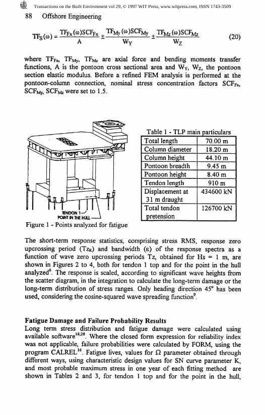
The methodology presented herein was applied to a TLP, considering thestress responses at the top of one tendon and at a point of the hull at theconnection of a pontoon to a column, both shown in Figure 1. The TLPstudied comprised 4 circular columns, 4 rectangular pontoons, without anyadditional brace, and the production deck, sized to work globally. Theplatform was designed to be anchored to seafloor in 938 m water depth by 12tendons (3 each corner). Its main characteristics are summarized in Table 1 .

Short term responseThe transfer functions and short-term responses of motions and stresses, wereobtained using SESAM system'*. The hydrodynamic model comprised a sink-source model, to calculate exciting body forces, added mass and potentialdamping, employing the radiation-diffraction theory; and a space frame modelto calculate drag forces through Morison formula, with drag coefficientsobtained from DNV Rules™. System inertia was given by sum of structuralmass, equipment, ballast, consumable, added mass and 1/3 of tendon mass,according to API-RP2T* for heave motions, applied at their tops as linear massin all directions. System damping was composed by potential damping andlinearized viscous damping. Besides the added buoyancy restoration at waterline, system stiffness is given mainly by tendons stiffness. Instead of using"straight line" tendon elements, it has been considered uncoupled linearizedvertical and horizontal spring constants, obtained from the expressions EA/Land T/L, respectively, where E is the elasticity modulus, A is the tendon crosssectional area, L is the tendon length and T is the tendon pretension, validatedfrom non-linear tendon analysis . Motion analyses were performed for allfrequencies in transfer functions and spaced incidence directions.

Transfer function of motion responses at a given point (TFp) is a linearcombination of TFs of motion responses at the origin of global coordinatessystem, taking into account the phase between them, given by

TFp(co) = TFnEAVE(tt) +yTFROLL(«>) - xTFpucH ) (19)

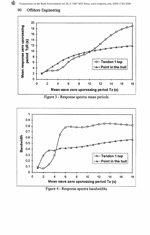
The displacements at tendon 1 top are transformed into stresses through theexpression S=EAL/L, AL being the tendon elongation. Inertia forces, obtainedby solving the equation of motions, and hydrodynamic forces were thentransferred to structural model to perform the quasi-static analysis. Thestructural model is a space frame including the hull and the deck truss. Thetransfer functions of stresses at the point in the hull, shown in Figure 3, wereobtained through the expression:



(20)

where TFpx, TFMy, TF\fe are axial force and bending moments transferfunctions, A is the pontoon cross sectional area and WY, Wz, the pontoonsection elastic modulus. Before a refined FEM analysis is performed at thepontoon-column connection, nominal stress concentration factors

y, SCFMz were set to 1.5.

TENDON i-/POINT IN THE HULL-

Figure 1 - Points analyzed for fatigue

Table 1 - TLP main particularsTotal lengthColumn diameterColumn heightPontoon breadthPontoon heightTendon lengthDisplacement at31m draughtTotal tendonpretension

70.00 m18.20m44.10m9.45m8.40m910m

434600 kN

126700 kN

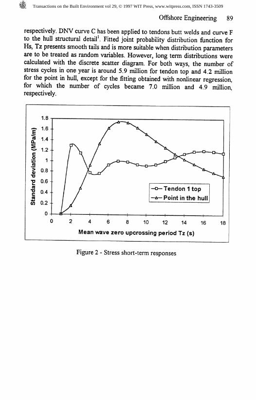
The short-term response statistics, comprising stress RMS, response zeroupcrossing period (TZR) and bandwidth (e) of the response spectra as afunction of wave zero upcrossing periods Tz, obtained for Hs = 1 m, areshown in Figures 2 to 4, both for tendon 1 top and for the point in the hullanalyzed*. The response is scaled, according to significant wave heights fromthe scatter diagram, in the integration to calculate the long-term damage or thelong-term distribution of stress ranges. Only heading direction 45** has beenused, considering the cosine-squared wave spreading function .

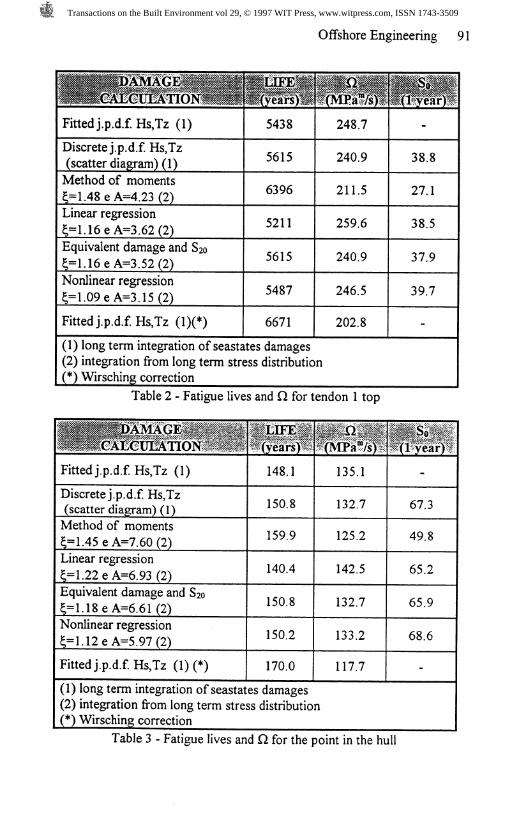
Fatigue Damage and Failure Probability ResultsLong term stress distribution and fatigue damage were calculated usingavailable software"***. Where the closed form expression for reliability indexwas not applicable, failure probabilities were calculated by FORM, using theprogram CALREL". Fatigue lives, values for Q parameter obtained throughdifferent ways, using characteristic design values for SN curve parameter K,and most probable maximum stress in one year of each fitting method areshown in Tables 2 and 3, for tendon 1 top and for the point in the hull,



respectively. DNV curve C has been applied to tendons butt welds and curve Fto the hull structural detail*. Fitted joint probability distribution function forHs, Tz presents smooth tails and is more suitable when distribution parametersare to be treated as random variables. However, long term distributions werecalculated with the discrete scatter diagram. For both ways, the number ofstress cycles in one year is around 5.9 million for tendon top and 4.2 millionfor the point in hull, except for the fitting obtained with nonlinear regression,for which the number of cycles became 7.0 million and 4.9 million,respectively.

Tendon 1 top

Point in the hull

2 4 6 8 10 12 14 16

Mean wave zero upcrossing period Tz (s)

Figure 2 - Stress short-term responses



•Tendon 1 top

-Point in the hull

2 4 6 8 10 12 14 16

Mean wave zero upcrossing period Tz (s)

18

Figure 3 - Response spectra mean periods

Tendon 1 top

Point in the hull

2 4 6 8 10 12 14 16Mean wave zero upcrossing period Tz (s)

Figure 4 - Response spectra bandwidths



Fitted j.p.df Hs,Tz (1) 5438 248.7

Discrete j.p.d.f. Hs,Tz(scatter diagram) (1) 5615 240.9 38.8

Method of moments£=1.48eA=4.23(2)

6396 211.5 27.1

Linear regression£=1.16eA=3.62(2)

5211 259.6 38.5

Equivalent damage and 820£=1.16eA=3.52(2)

5615 240.9 37.9

Nonlinear regression£=1.09eA=3.15(2)

5487 246.5 39.7

Fitted j.p.d.f. Hsjz (!)(*) 6671 202.8

(1) long term integration of seastates damages(2) integration from long term stress distribution(*) Wirsching correction

Table 2 - Fatigue lives and Q for tendon 1 top

Fitted j.p.d.f. Hsjz (1) 148.1 135.1

Discrete j.p.d.f. Hs,Tz(scatter diagram) (1) 150.8 132.7 67.3

Method of moments£=1.45eA=7.60(2)

159.9 125.2 49.8

Linear regression£=1.22eA=6.93(2)

140.4 142.5 65.2

Equivalent damage and 820t=1.18eA=6.61 (2) 150.8 132.7 65.9

Nonlinear regression£=1.12eA=5.97(2) 150.2 133.2 68.6

Fitted j.p.d.f. Hsjz (!)(*) 170.0 117.7

(1) long term integration of seastates damages(2) integration from long term stress distribution(*) Wirsching correction

Table 3 - Fatigue lives and Q, for the point in the hull



-o—Sum-Rayleigh-H— Method of moments-o—Linear regression-A—Equivalent D and S20-H—Nonlinear regression

1.0E+00 1.0E+01 1.0E+02 1.0E+03 1.0E+04 1.0E+05 1.0E+06 1.0E+07

Number of cycles

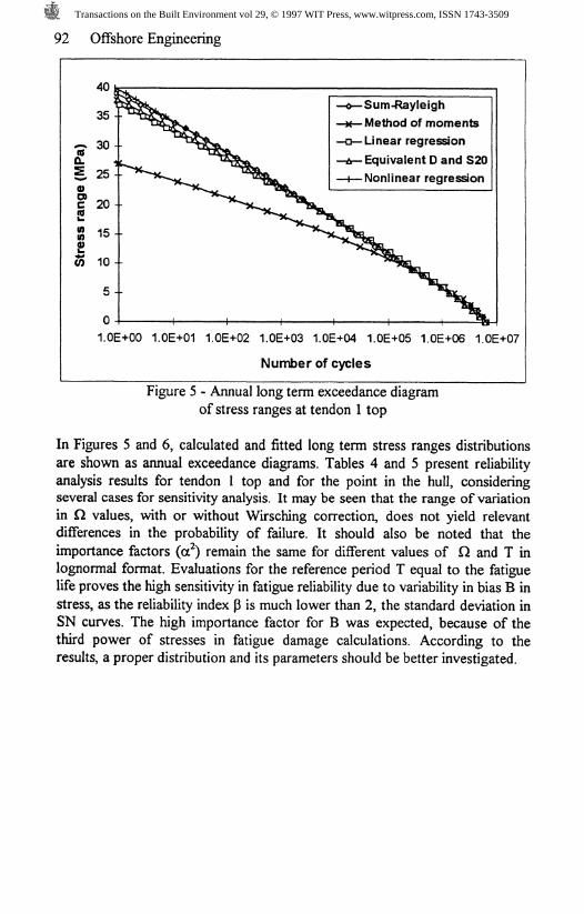
Figure 5 - Annual long term exceedance diagramof stress ranges at tendon 1 top

In Figures 5 and 6, calculated and fitted long term stress ranges distributionsare shown as annual exceedance diagrams. Tables 4 and 5 present reliabilityanalysis results for tendon 1 top and for the point in the hull, consideringseveral cases for sensitivity analysis. It may be seen that the range of variationin Q values, with or without Wirsching correction, does not yield relevantdifferences in the probability of failure. It should also be noted that theimportance factors (of) remain the same for different values of Q and T inlognormal format. Evaluations for the reference period T equal to the fatiguelife proves the high sensitivity in fatigue reliability due to variability in bias B instress, as the reliability index p is much lower than 2, the standard deviation inSN curves. The high importance factor for B was expected, because of thethird power of stresses in fatigue damage calculations. According to theresults, a proper distribution and its parameters should be better investigated.



Sum-Rayleigh

Method of moments

Linear regressionEquivalent D and S20

Nonlinear regression

1.0E+00 1.0E+01 1.0E+02 1.0E+03 1.0E+04 1.0E+05 1.0E+06 1.0E+07

Number of cycles

Figure 6 - annual long term exceedance diagramof stress ranges at the point in the hull

14,034 1,0 1,00,2041 0,5 0,5

n = 248.7T = 20 years

13,83 4,78 0,554-1,008 3,546 -1,0133,82 pf 6,58x10^

£1 = 202.8T = 20 years

13,82 5,02 0,546-1,038 3,652 -1,0443,94 pf 4,11x10'*

n = 248.7T=5438 years

14,00 1,204 0,822-0,179 0,630 -0,1800,679 _EL 2,49x10-1

a 0,070 0,860 0,070

n = 248.7T = 20 years

13,44 2,87 0,227-2,890 3,746 -2,905

3 5,55 .PL 1,41x10*a 0,271 0,455 0,274

Table 4 - Reliability results for tendon 1 top



12,237 1,0 1,00,2183 0,5 0,5

n =135,1T =20 years

12,09

-0,6542,0503

2,137

1,8440,669

-0,6152,02x10"

Q= 117,7T = 20 years

12,09

-0,6822,1378

2,218

1,922

pf

0,661-0,6411,63x10"

D =135,1T = 148 years

12,18

-0,2490,780

1,246

0,7010,801

-0,2342,18x10''

a 0,102 0,808 0,090

n= 135.1T = 20 years

12,00

-1,0832,2824

1,866

1,7320,553

-1,0181,12x10"

a 0,225 0,576 0,199

/Snablesl

12,237 1,0 1,00,2183 0,3 0,5%<###%%%*•%!ormail

n =135,1T = 20 years

11,97-1,2152,705

1,7902,130

Pf

0,521-1,1423,42x10"

0,202 0,620 0,178

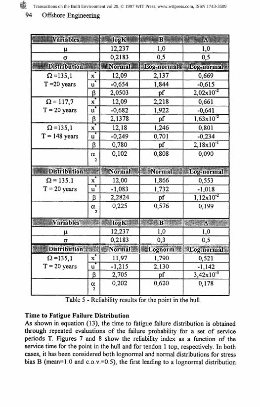
Table 5 - Reliability results for the point in the hull

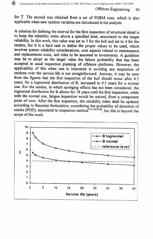
Time to Fatigue Failure DistributionAs shown in equation (13), the time to fatigue failure distribution is obtainedthrough repeated evaluations of the failure probability for a set of serviceperiods T Figures 7 and 8 show the reliability index as a function of theservice time for the point in the hull and for tendon 1 top, respectively. In bothcases, it has been considered both lognormal and normal distributions for stressbias B (mean=1.0 and c.o.v.=0.5), the first leading to a lognormal distribution



for T. The second was obtained from a set of FORM runs, which is alsoapplicable when new random variables are introduced in the analysis.

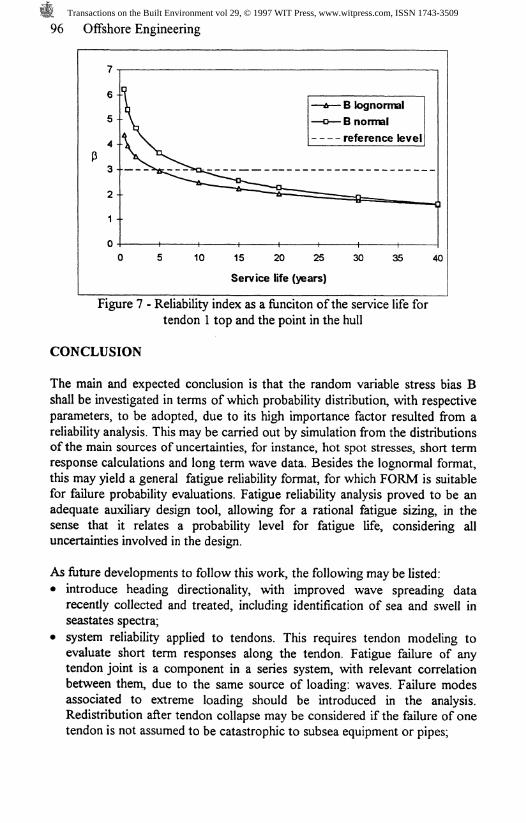
A criterion for defining the interval for the first inspection of structural detail isto keep the reliability index above a specified limit, associated to the targetreliability. In this work, this value was set to 3 for the hull and set to 4 for thetendon, but it is a hard task to define the proper values to be used, whichinvolves system reliability considerations, cost aspects related to maintenanceand replacements costs, and risks to be assumed in investments. A guidelinemay be to adopt as the target value the failure probability that has beenaccepted in usual inspection planning of offshore platforms. However, theapplicability of this when one is interested in avoiding any inspection oftendons over the service life is not straightforward. Anyway, it may be seenfrom the figures that the first inspection of the hull should occur after 4.5years, for a lognormal distribution of B, increased to 9.5 years for a normalone. For the tendon, in which springing effects has not been considered, thelognormal distribution for B allows for 18 years until the first inspection, whilewith the normal one, fatigue inspection would be waived, from a componentpoint of view. After the first inspection, the reliability index shall be updatedaccording to Bayesian formulation, considering the probability of detection ofcracks (POD), associated to inspection method*'"'"*"**, but this is beyond thescope of this work.

B lognormal

B normal

reference level

15 20 25

Service life (years)



•— B lognormalt— B normal-- reference level

15 20 25

Service life (years)

Figure 7 - Reliability index as a funciton of the service life fortendon 1 top and the point in the hull

CONCLUSION

The main and expected conclusion is that the random variable stress bias Bshall be investigated in terms of which probability distribution, with respectiveparameters, to be adopted, due to its high importance factor resulted from areliability analysis. This may be carried out by simulation from the distributionsof the main sources of uncertainties, for instance, hot spot stresses, short termresponse calculations and long term wave data. Besides the lognormal format,this may yield a general fatigue reliability format, for which FORM is suitablefor failure probability evaluations. Fatigue reliability analysis proved to be anadequate auxiliary design tool, allowing for a rational fatigue sizing, in thesense that it relates a probability level for fatigue life, considering alluncertainties involved in the design.

As future developments to follow this work, the following may be listed:• introduce heading directionality, with improved wave spreading data

recently collected and treated, including identification of sea and swell inseastates spectra;

• system reliability applied to tendons. This requires tendon modeling toevaluate short term responses along the tendon. Fatigue failure of anytendon joint is a component in a series system, with relevant correlationbetween them, due to the same source of loading: waves. Failure modesassociated to extreme loading should be introduced in the analysis.Redistribution after tendon collapse may be considered if the failure of onetendon is not assumed to be catastrophic to sub sea equipment or pipes;



springing effects should be taken into account, with special attention todamping of the system at resonance. Model testing is thought to be still thebest way to evaluate the response at sum-frequency, although someanalytical models have been proposed;

target reliability is to be determined taking into account consequences of aneventual system failure, in terms of insurance, replacement and fine costs,and structure characteristics, concerning redundancy and field behaviorknowledge;updating reliability from inspection results;

REFERENCES

[1] Almar-Naess, A., 1985, Fatigue Handbook: Offshore Steel Structures,Trondheim, Tapir.

[2] Alves, Luiz H. M, 1996, "Dynamic Analysis of the Tendons of a TensionLeg Platform", M.Sc. Thesis, PEC COPPE/UFRJ, Rio de Janeiro.

[3] API (American Petroleum Institute), 1987, Recommended Practice forPlanning, Designing and Constructing Tension Leg Platforms (RP 2T),First edition.

[4] ASCE, 1982% "Fatigue Reliability: Introduction", Journal of theStructural Division, Vol. 108, No. STL

[5] ASCE, 1982b, "Fatigue Reliability: Quality Assurance andMaintainability", Journal of the Structural Division, Vol. 108, No. STL

[6] Bardanachvili, C.A., 1996, "Fatigue Reliability of Tension Leg Platforms(TLP)," M.Sc. Thesis, PEC COPPE/UFRJ, Rio de Janeiro.

[7] Bardanachvili, C.A., Lima, E.C., Sagrilo, L.V., and Ellwanger, G.B.,1997, "Fatigue Reliability of a Tension Leg Platform for Campos Basin",Proc. ofOMAE'97.

[8] Branco, CM, Fernandes, A.A., Castro, P.M.S., 1986, Fadiga deEstruturas Soldadas, Funda^ao Calouste Gulbenkian, Lisbon.

[9] DNV (Det Norske Veritas), 1984, Fatigue Strength Analysis for MobileOffshore Units, Classification Notes, No. 30.2.

[10] DNV (Det Norske Veritas), 1990, Rules for Classification of MobileOffshore Units, P. 3, Ch. 1, Structural Design General.

[11] DNV (Det Norske Veritas), 1992, Structural Reliability Analysis ofMarine Structures, Classification Notes, No. 30.6.

[12] DNV (Det Norske Veritas), 1994, SESAM User's Manuals, Latestrevisions.

[13] Jiao, G., Moan, T., and Marley, M. J., 1990, "Reliability Analysis of TLPTether Systems," Proc. OMAE 90.

[14]Kirkemo, F., 1988, "Applications of Probabilistic Fracture Mechanics toOffshore Structures," DNV, Paper Series, No. 87 P210.



f!5]Kujawski, D., and Ellyin, F., 1995, "A unified approach to mean stresseffect on fatigue threshold conditions." IntemationalJ. Fatigue, Vol. 17,No. 2, pp. 101-106..

[16] Liu, P.-L., Lin, H.-Z., and Der Kiureghian, A., 1989, CALREL User'sManual, Department of Civil engineering, University of California atBerkeley, USA.

[17]Madsen, H.O., Krenk, S., and Lind, N.C., 1986, Methods of StructuralSafety, Prentice-Hall, Inc., Englewood Cliffs, New Jersey.

[18] Mathsoft Inc., 1994, MATHCAD 5.0 Users Manual.[19] Moan, T., 1993, "Reliability and risk analysis for design and operations

planning of offshore structures", Structural Safety & Reliability,ICOSSAR.

[20] PETROBRAS, 1995, "Metocean, Soil Data and Bathymetry Chart",Technical Specification ET-3010.32-1200-94l-PPC-001.

[21]Pittaluga, A., Cazzulo, R., and Romeo, P., 1991, "Uncertainties in theFatigue Design of Offshore Steel Structures", Marine Structures, Vol. 4.

[22] Price, W.G., and Bishop, R.E.D.,1974, Probabilistic Theory of ShipDynamics, Chapman and Hall, Londres.

[23] Shanks, J.M., and Lim, F.K., 1987, "TLP Tether Fatigue AssessmentIncorporating Bending Response and Long Term Wave Directionality",Proc. OMAE87, Voll.

[24] Shive, A.R., Brewer, J.H., and Vora, MR., 1990, "Preliminary Design ofTendons for Deepwater TLP's", OTC, No. 6448.

[25] Siqueira, M.Q., 1995, "Random Analysis of Offshore Structures: Shortand Long Term Statistics and Determination of Extremes Values", D.Sc.Thesis, COPPE/UFRJ, Rio de Janeiro.

[26] Skjong, R., and Torhaug, R., 1991, "Rational Methods for Fatigue Designand Inspection Planning of Offshore Structures", Marine Structures, Vol.4.

[27] Soares, C.G., and Moan, T., 1991, "Model Uncertainty in the Long-termDistribution of Wave-induced Bending Moments for Fatigue Design ofShip Structures", Marine Structures, Vol. 4.

[28] Statistical Graphics Corporation, STATGRAPfflCS 4.0 User's Manual,1989.

[29] Wirsching, P.H., 1979, "Fatigue Reliability in Welded Joints of OffshoreStructures", OTC.

[30] Wirsching, P.H. et al., 1982, "Fatigue Reliability: Variable AmplitudeLoading", Journal of the Structural Division (ASCE), Vol. 108, No. ST1.

[31]Zimmermann, J.J., and Banon, H., 1994, "System Fatigue Reliability andInspection Planning for Offshore Platforms", Proc. OMAE 94.


Documents

DETERMINATION OF LONG TERM DISTRIBUTION OF PETROBRAS ... · PETROBRAS/CENPES Edison C. P. de Lima, Luis V. S. Sagrilo and Gilberto B. Ellwanger COPPE/UFRJ Abstract — The tension