Determinants of Capital Inflows: New Empirical Evidence … · 2017-11-30 · 1 Determinants of Capital Inflows: New Empirical Evidence Introduction The simplest benchmark neoclassical

1

Determinants of Capital Inflows: New Empirical Evidence

Introduction

The simplest benchmark neoclassical growth model (e.g. Solow, 1956) suggests that capital should

flow from capital-rich developed countries to capital-poor developing countries as a result of

‘diminishing returns to capital’. Lucas (1990) points out in his classic article that neoclassical

assumptions on technology and trade in goods and factors are ‘drastically wrong’ and poses the

provocative question “Why Doesn’t Capital Flow from Rich to Poor Countries?” (Lucas 1990, p. 92).

This puzzle, known as the ‘Lucas Paradox’-the lack of capital flows from rich to poor countries-,

introduced a new debate and spawned an extensive literature. From Lucas’s point of view, differences

in ‘fundamentals’, such as human capital between rich and poor countries potentially explain this

paradox. Lucas rejects capital market imperfection or political risk as an explanation for the lower

capital flows to poor countries, pointing to the fact that before World War II many of today’s poor

countries were colonies and subject to rich countries laws and governing institutions.

Empirical investigations of the Lucas paradox draw dramatically different conclusions concerning its

key determinants. However, these alternative explanations of the Lucas paradox based on empirical

models that focus on fairly narrow channels of the determinants of capital inflows, and in some cases

model misspecification is partially responsible for inconclusive findings. For example, Alfaro,

Kalemli-Ozcan, and Volosovych (2008) claim to provide a definite answer to this paradox and

conclude that, differences in institutional quality determine capital inflows and can fully explain

Lucas paradox. Papaioannou (2009) reaches a similar conclusion using bilateral bank inflows.

Specific aspects of institutional quality have also been considered in the empirical literature, and

economically significant barriers to foreign investment include government corruption (Wei, 2000)

and default risk (Reinhart and Rogoff, 2004). However, Okada (2012) finds that institutional quality

cannot independently provide an answer to the Lucas paradox when estimating a dynamic model;

instead the interaction between institutional quality and financial openness can. Several other studies

have also pointed to the importance of capital market frictions, such as capital controls as barriers to

international capital movements (Henry, 2007; Abiad, Leigh, and Mody 2009; and Reinhardt, Ricci,

and Tressel, 2013), as well as financial development (Forbes, 2010; Von Hagen and Zhang, 2010)1.

Several other studies found that other types of frictions, such as information asymmetries matter for

capital inflows (Portes and Rey, 2005; Hashimoto and Wacker, 2012). Finally, there is empirical

evidence pointing to economic fundamentals as primary factors in explaining international capital

1 Additional evidence that financial frictions matter more generally is offered by Kalemli-Ozcan et al. (2010),

who estimate a simple version of the standard neoclassical open economy model using within country capital

flow data for US states. They find that capital flows from slow-growing to fast-growing states, in line with the

theory, and that the simple model explains a large proportion of within country variation, suggesting that

barriers at the border that prevent international capital flows.

2

flows. Clemens and Williamson (2004), for example, study the first era of financial integration (1870-

1913), examining British capital flows to 34 capital recipients, and find countries with higher average

schooling, urbanization, and migration rates attract more foreign capital. By contrast, Gourinchas and

Jeanne (2013) find faster productivity growth negatively affects capital inflows, meaning that capital

does not flow to high-growth countries, a finding opposite to the neoclassical prediction.

In this paper, we empirically examine the relative importance of factors from all three broad

categories (institutions, frictions, and fundamentals) in explaining Lucas’ paradox.2 Specifically, in

modelling international capital flows, we consider a variety of potential determinants spanning all

categories and, by examining the statistical significance of economic development in all models, we

ask: which combinations of factors account for the Lucas paradox- the positive correlation between

economic development and capital inflows? We find there is no magic bullet solution to the Lucas

paradox, although this is often claimed in the empirical literature. Initial economic development

(measured by log initial GDP per capita) is driving force of capital inflows in all models. Stocks of

human capital, institutional qualities, and financial openness are also statistically significant

determinants. However, none of these determinants can independently fully account for the positive

relationship between economic development and capital inflows.

This paper is organized as follows. Section II reviews the determinants of capital inflows in the

standard neoclassical model. Section III replicates closely related empirical work and points to the

limitations of the models used. Section IV re-specifies the empirical model and produces new

empirical findings using an updated dataset. Section V concludes.

Section II

Background

Theoretical issues: Before discussing the empirical specifications, we review the standard

neoclassical model and show how differences in fundamentals, institutions, and frictions in the

financial sector are represented in such a model. Consider a small open economy that uses capital (K)

and labour (L) to produce output (Y) with constant returns to scale. For simplicity, we start from the

production function:

( ) (1)

2 As some observed factors do not fit neatly into a single category, this categorization is not mutually exclusive.

3

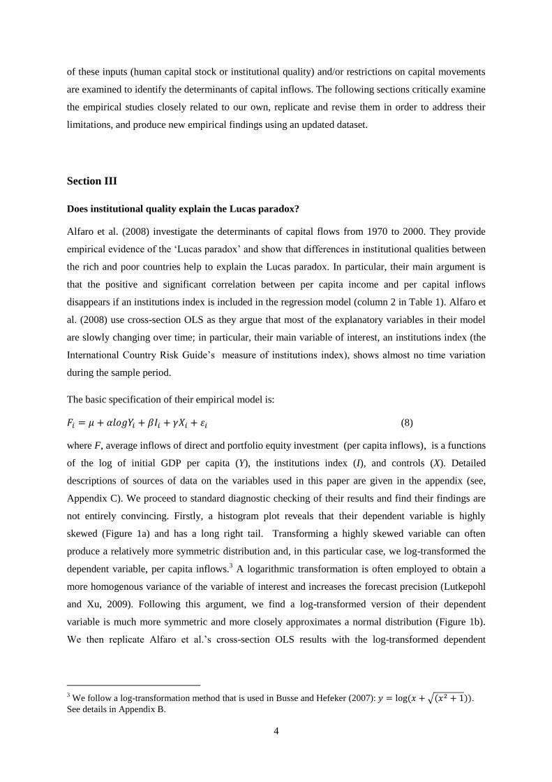
The per capita production function from equation (1), including a technology parameter or shift

parameter (A) that represents total factor productivity, can be expressed as follows:

(

) (2)

( ) (3)

Where, lower case letters denote quantities per capita. Consider two countries i and j where, i≠j and

the marginal products of capital are equal to the returns to capital (r) in each country:

( ) (4)

( ) (5)

Neoclassical theory suggests that capital should flow from capital-abundant countries to capital-scarce

countries, based on diminishing returns to capital, before equalization takes place. In this set-up,

consider the case where the marginal productivity of capital is higher in country i (capital-scare) than

in country j (capital-abundant). Assuming that capital is perfectly mobile across countries, capital

flows from country j to country i and the returns to capital are equalized with the global risk-free rate

of return (r) implying that:

In a panel set up, we can write this equation:

( )

( ) (6)

However, there are other factors, such as ‘human capital stock’(represented here by human capital per

capita, h) (e.g. Lucas, 1990), differences in institutional quality (θ) (e.g. Alfaro et al., 2008), and

frictions in capital markets (τ) (e.g. Reinhardt et al., 2013) that constitute a wedge between expected

and ex-post returns to capital and influence this equality condition. If we incorporate these inputs and

capital market imperfections in the neoclassical model the counterpart of equation (6) can be

expressed as, similar to Alfaro et al.’s (2008) equation (5):

( ( )) ( ) ( ( ))

( ) (7)

Equation (7) suggests the ex-post returns to capital are adjusted for the human capital stock,

institutional quality, and capital market imperfections. In particular, a higher stock of human capital

raises the marginal productivity of capital, a lower level of institutional quality, for example due to

expropriation risk and/or higher corruption reduces the marginal productivity of capital, and a higher

level of restrictions on capital movements causes an inefficient allocation and increases the cost of

capital and reduces the marginal productivity of capital. In the existing empirical literature, the effects

4

of these inputs (human capital stock or institutional quality) and/or restrictions on capital movements

are examined to identify the determinants of capital inflows. The following sections critically examine

the empirical studies closely related to our own, replicate and revise them in order to address their

limitations, and produce new empirical findings using an updated dataset.

Section III

Does institutional quality explain the Lucas paradox?

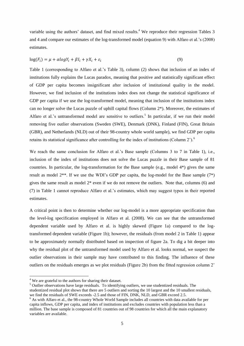
Alfaro et al. (2008) investigate the determinants of capital flows from 1970 to 2000. They provide

empirical evidence of the ‘Lucas paradox’ and show that differences in institutional qualities between

the rich and poor countries help to explain the Lucas paradox. In particular, their main argument is

that the positive and significant correlation between per capita income and per capital inflows

disappears if an institutions index is included in the regression model (column 2 in Table 1). Alfaro et

al. (2008) use cross-section OLS as they argue that most of the explanatory variables in their model

are slowly changing over time; in particular, their main variable of interest, an institutions index (the

International Country Risk Guide’s measure of institutions index), shows almost no time variation

during the sample period.

The basic specification of their empirical model is:

(8)

where F, average inflows of direct and portfolio equity investment (per capita inflows), is a functions

of the log of initial GDP per capita (Y), the institutions index (I), and controls (X). Detailed

descriptions of sources of data on the variables used in this paper are given in the appendix (see,

Appendix C). We proceed to standard diagnostic checking of their results and find their findings are

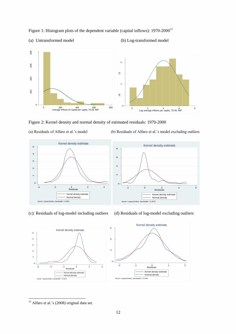
not entirely convincing. Firstly, a histogram plot reveals that their dependent variable is highly

skewed (Figure 1a) and has a long right tail. Transforming a highly skewed variable can often

produce a relatively more symmetric distribution and, in this particular case, we log-transformed the

dependent variable, per capita inflows.3 A logarithmic transformation is often employed to obtain a

more homogenous variance of the variable of interest and increases the forecast precision (Lutkepohl

and Xu, 2009). Following this argument, we find a log-transformed version of their dependent

variable is much more symmetric and more closely approximates a normal distribution (Figure 1b).

We then replicate Alfaro et al.’s cross-section OLS results with the log-transformed dependent

3 We follow a log-transformation method that is used in Busse and Hefeker (2007): ( √( )).

See details in Appendix B.

5

variable using the authors’ dataset, and find mixed results.4 We reproduce their regression Tables 3

and 4 and compare our estimates of the log-transformed model (equation 9) with Alfaro et al.’s (2008)

estimates.

( ) (9)

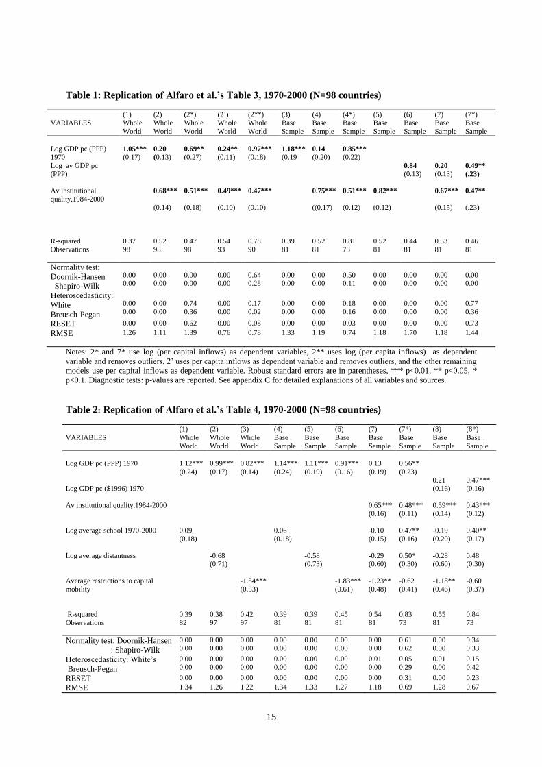
Table 1 (corresponding to Alfaro et al.’s Table 3), column (2) shows that inclusion of an index of

institutions fully explains the Lucas paradox, meaning that positive and statistically significant effect

of GDP per capita becomes insignificant after inclusion of institutional quality in the model.

However, we find inclusion of the institutions index does not change the statistical significance of

GDP per capita if we use the log-transformed model, meaning that inclusion of the institutions index

can no longer solve the Lucas puzzle of uphill capital flows (Column 2*). Moreover, the estimates of

Alfaro et al.’s untransformed model are sensitive to outliers.5 In particular, if we run their model

removing five outlier observations (Sweden (SWE), Denmark (DNK), Finland (FIN), Great Britain

(GBR), and Netherlands (NLD) out of their 98-country whole world sample), we find GDP per capita

retains its statistical significance after controlling for the index of institutions (Column 2’).6

We reach the same conclusion for Alfaro et al.’s Base sample (Columns 3 to 7 in Table 1), i.e.,

inclusion of the index of institutions does not solve the Lucas puzzle in their Base sample of 81

countries. In particular, the log-transformation for the Base sample (e.g., model 4*) gives the same

result as model 2**. If we use the WDI’s GDP per capita, the log-model for the Base sample (7*)

gives the same result as model 2* even if we do not remove the outliers. Note that, columns (6) and

(7) in Table 1 cannot reproduce Alfaro et al.’s estimates, which may suggest typos in their reported

estimates.

A critical point is then to determine whether our log-model is a more appropriate specification than

the level-log specification employed in Alfaro et al. (2008). We can see that the untransformed

dependent variable used by Alfaro et al. is highly skewed (Figure 1a) compared to the log-

transformed dependent variable (Figure 1b); however, the residuals (from model 2 in Table 1) appear

to be approximately normally distributed based on inspection of figure 2a. To dig a bit deeper into

why the residual plot of the untransformed model used by Alfaro et al. looks normal, we suspect the

outlier observations in their sample may have contributed to this finding. The influence of these

outliers on the residuals emerges as we plot residuals (Figure 2b) from the fitted regression column 2’

4 We are grateful to the authors for sharing their dataset.

5 Outlier observations have large residuals. To identifying outliers, we use studentized residuals. The

studentized residual plot shows that there are 5 outliers and sorting the 10 largest and the 10 smallest residuals,

we find the residuals of SWE exceeds -2.5 and those of FIN, DNK, NLD, and GBR exceed 2.5. 6 As with Alfaro et al., the 98-country Whole World Sample includes all countries with data available for per

capita inflows, GDP per capita, and index of institutions and excludes countries with population less than a

million. The base sample is composed of 81 countries out of 98 countries for which all the main explanatory

variables are available.

6

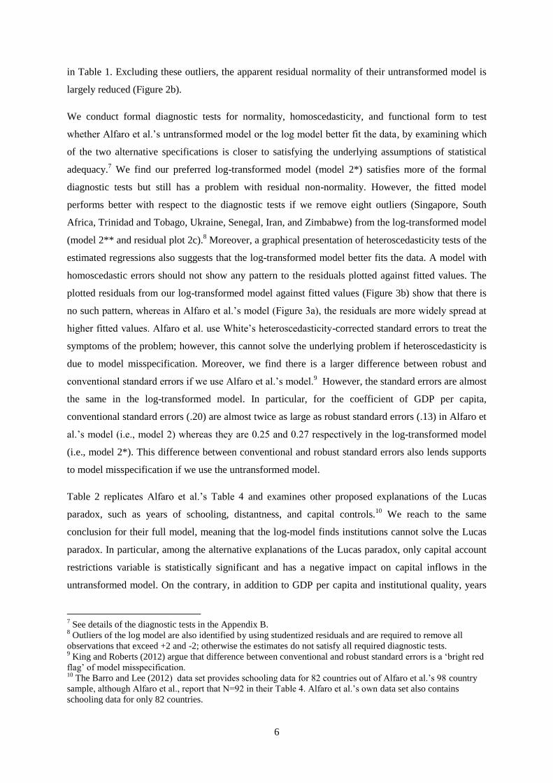
in Table 1. Excluding these outliers, the apparent residual normality of their untransformed model is

largely reduced (Figure 2b).

We conduct formal diagnostic tests for normality, homoscedasticity, and functional form to test

whether Alfaro et al.’s untransformed model or the log model better fit the data, by examining which

of the two alternative specifications is closer to satisfying the underlying assumptions of statistical

adequacy.7 We find our preferred log-transformed model (model 2*) satisfies more of the formal

diagnostic tests but still has a problem with residual non-normality. However, the fitted model

performs better with respect to the diagnostic tests if we remove eight outliers (Singapore, South

Africa, Trinidad and Tobago, Ukraine, Senegal, Iran, and Zimbabwe) from the log-transformed model

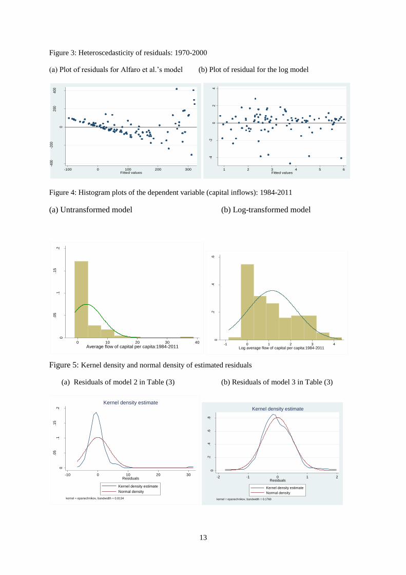
(model 2** and residual plot 2c).8 Moreover, a graphical presentation of heteroscedasticity tests of the

estimated regressions also suggests that the log-transformed model better fits the data. A model with

homoscedastic errors should not show any pattern to the residuals plotted against fitted values. The

plotted residuals from our log-transformed model against fitted values (Figure 3b) show that there is

no such pattern, whereas in Alfaro et al.’s model (Figure 3a), the residuals are more widely spread at

higher fitted values. Alfaro et al. use White’s heteroscedasticity-corrected standard errors to treat the

symptoms of the problem; however, this cannot solve the underlying problem if heteroscedasticity is

due to model misspecification. Moreover, we find there is a larger difference between robust and

conventional standard errors if we use Alfaro et al.’s model.9 However, the standard errors are almost

the same in the log-transformed model. In particular, for the coefficient of GDP per capita,

conventional standard errors (.20) are almost twice as large as robust standard errors (.13) in Alfaro et

al.’s model (i.e., model 2) whereas they are 0.25 and 0.27 respectively in the log-transformed model

(i.e., model 2*). This difference between conventional and robust standard errors also lends supports

to model misspecification if we use the untransformed model.

Table 2 replicates Alfaro et al.’s Table 4 and examines other proposed explanations of the Lucas

paradox, such as years of schooling, distantness, and capital controls.10

We reach to the same

conclusion for their full model, meaning that the log-model finds institutions cannot solve the Lucas

paradox. In particular, among the alternative explanations of the Lucas paradox, only capital account

restrictions variable is statistically significant and has a negative impact on capital inflows in the

untransformed model. On the contrary, in addition to GDP per capita and institutional quality, years

7 See details of the diagnostic tests in the Appendix B.

8 Outliers of the log model are also identified by using studentized residuals and are required to remove all

observations that exceed +2 and -2; otherwise the estimates do not satisfy all required diagnostic tests. 9 King and Roberts (2012) argue that difference between conventional and robust standard errors is a ‘bright red

flag’ of model misspecification. 10

The Barro and Lee (2012) data set provides schooling data for 82 countries out of Alfaro et al.’s 98 country

sample, although Alfaro et al., report that N=92 in their Table 4. Alfaro et al.’s own data set also contains

schooling data for only 82 countries.

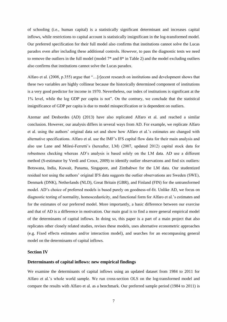
7

of schooling (i.e., human capital) is a statistically significant determinant and increases capital

inflows, while restrictions to capital account is statistically insignificant in the log-transformed model.

Our preferred specification for their full model also confirms that institutions cannot solve the Lucas

paradox even after including these additional controls. However, to pass the diagnostic tests we need

to remove the outliers in the full model (model 7* and 8* in Table 2) and the model excluding outliers

also confirms that institutions cannot solve the Lucas paradox.

Alfaro et al. (2008, p.355) argue that “....[r]ecent research on institutions and development shows that

these two variables are highly collinear because the historically determined component of institutions

is a very good predictor for income in 1970. Nevertheless, our index of institutions is significant at the

1% level, while the log GDP per capita is not”. On the contrary, we conclude that the statistical

insignificance of GDP per capita is due to model misspecification or is dependent on outliers.

Azemar and Desbordes (AD) (2013) have also replicated Alfaro et al. and reached a similar

conclusion. However, our analysis differs in several ways from AD. For example, we replicate Alfaro

et al. using the authors’ original data set and show how Alfaro et al.’s estimates are changed with

alternative specifications. Alfaro et al. use the IMF’s IFS capital flow data for their main analysis and

also use Lane and Milesi-Ferretti’s (hereafter, LM) (2007, updated 2012) capital stock data for

robustness checking whereas AD’s analysis is based solely on the LM data. AD use a different

method (S-estimator by Verdi and Croux, 2009) to identify outlier observations and find six outliers:

Botswana, India, Kuwait, Panama, Singapore, and Zimbabwe for the LM data. Our studentized

residual test using the authors’ original IFS data suggests the outlier observations are Sweden (SWE),

Denmark (DNK), Netherlands (NLD), Great Britain (GBR), and Finland (FIN) for the untransformed

model. AD’s choice of preferred models is based purely on goodness-of-fit. Unlike AD, we focus on

diagnostic testing of normality, homoscedasticity, and functional form for Alfaro et al.’s estimates and

for the estimates of our preferred model. More importantly, a basic difference between our exercise

and that of AD is a difference in motivation. Our main goal is to find a more general empirical model

of the determinants of capital inflows. In doing so, this paper is a part of a main project that also

replicates other closely related studies, revises these models, uses alternative econometric approaches

(e.g. Fixed effects estimates and/or interaction model), and searches for an encompassing general

model on the determinants of capital inflows.

Section IV

Determinants of capital inflows: new empirical findings

We examine the determinants of capital inflows using an updated dataset from 1984 to 2011 for

Alfaro et al.’s whole world sample. We run cross-section OLS on the log-transformed model and

compare the results with Alfaro et al. as a benchmark. Our preferred sample period (1984 to 2011) is

8

not having missing observations of annual data for the institutions index for this full period, the main

variable of interest. In comparison, Alfaro et al.’s sample period is from 1970 to 2000 whereas the

ICRG’s institutions index is available only from 1984. Alfaro et al.’s estimates are based solely on

ICRG’s index of institutions, whereas other indices are often used to measure institutional quality,

such as the Freedom House Index, Transparency International’s CPI (corruption perception index),

World Bank’s CPIA (Country policy and institutions assessments) index, and the World Bank

Institute’s Governance Indicators (Kaufmann et al., 1996, updated 2011). We argue that a perfect

institutions index will undoubtedly never exist and we acknowledge the complexities of using such

indices for cross-country comparisons suggesting us to use an alternative measure of institutional

quality to examine whether our findings are robust. Therefore, we also use the WBI’s governance

index in addition to the ICRG’s institutions index.

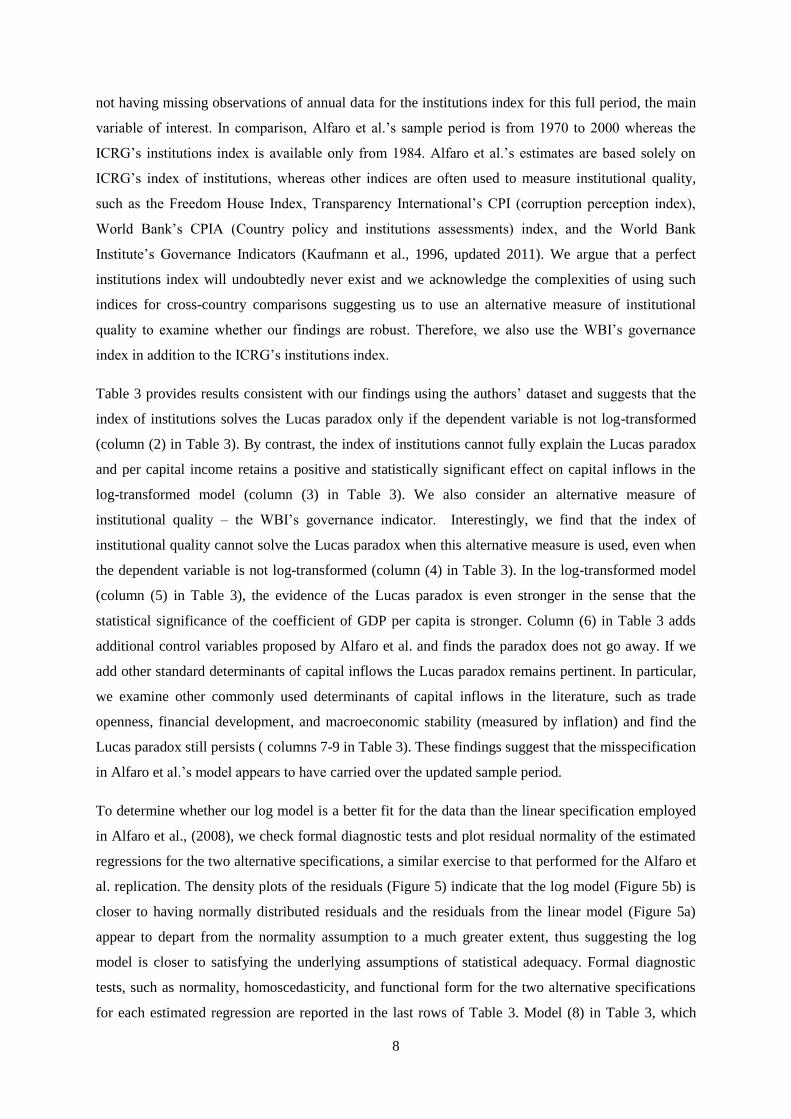
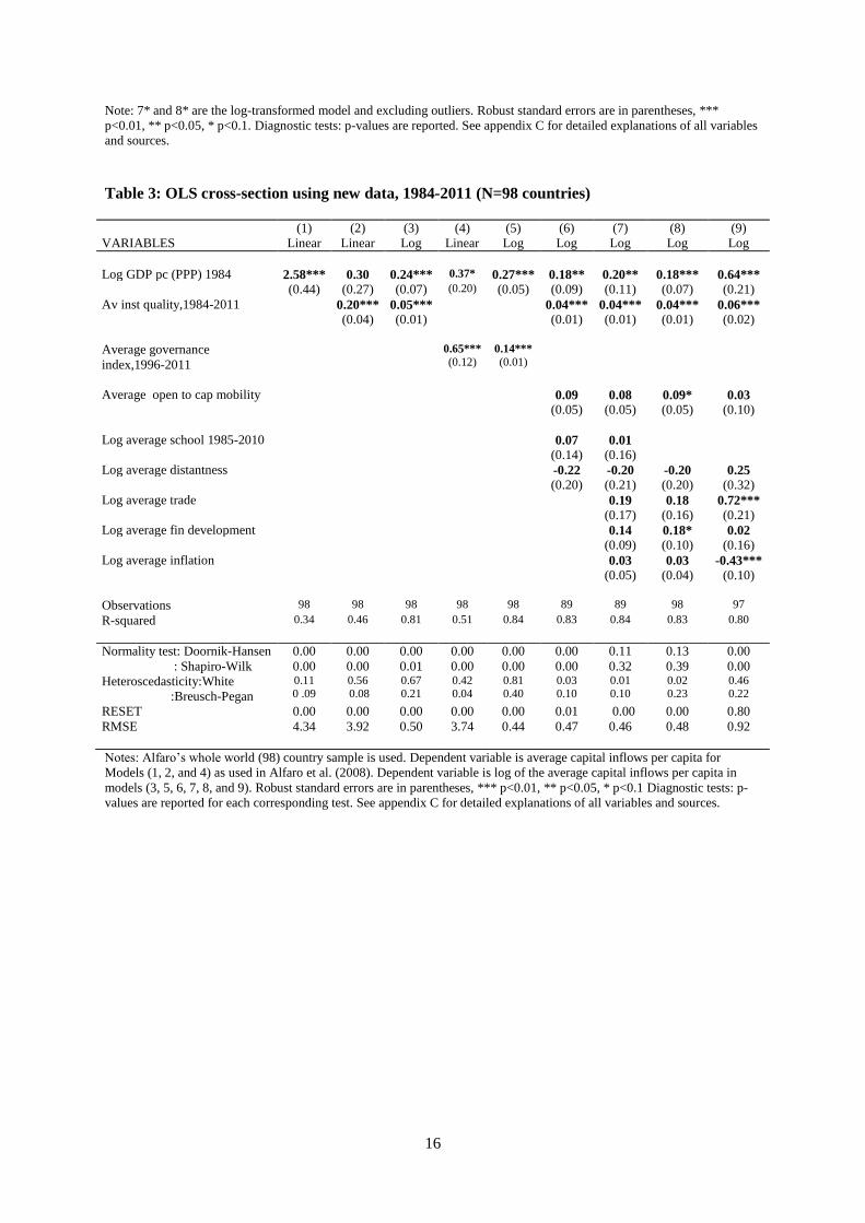
Table 3 provides results consistent with our findings using the authors’ dataset and suggests that the

index of institutions solves the Lucas paradox only if the dependent variable is not log-transformed

(column (2) in Table 3). By contrast, the index of institutions cannot fully explain the Lucas paradox

and per capital income retains a positive and statistically significant effect on capital inflows in the

log-transformed model (column (3) in Table 3). We also consider an alternative measure of

institutional quality – the WBI’s governance indicator. Interestingly, we find that the index of

institutional quality cannot solve the Lucas paradox when this alternative measure is used, even when

the dependent variable is not log-transformed (column (4) in Table 3). In the log-transformed model

(column (5) in Table 3), the evidence of the Lucas paradox is even stronger in the sense that the

statistical significance of the coefficient of GDP per capita is stronger. Column (6) in Table 3 adds

additional control variables proposed by Alfaro et al. and finds the paradox does not go away. If we

add other standard determinants of capital inflows the Lucas paradox remains pertinent. In particular,

we examine other commonly used determinants of capital inflows in the literature, such as trade

openness, financial development, and macroeconomic stability (measured by inflation) and find the

Lucas paradox still persists ( columns 7-9 in Table 3). These findings suggest that the misspecification

in Alfaro et al.’s model appears to have carried over the updated sample period.

To determine whether our log model is a better fit for the data than the linear specification employed

in Alfaro et al., (2008), we check formal diagnostic tests and plot residual normality of the estimated

regressions for the two alternative specifications, a similar exercise to that performed for the Alfaro et

al. replication. The density plots of the residuals (Figure 5) indicate that the log model (Figure 5b) is

closer to having normally distributed residuals and the residuals from the linear model (Figure 5a)

appear to depart from the normality assumption to a much greater extent, thus suggesting the log

model is closer to satisfying the underlying assumptions of statistical adequacy. Formal diagnostic

tests, such as normality, homoscedasticity, and functional form for the two alternative specifications

for each estimated regression are reported in the last rows of Table 3. Model (8) in Table 3, which

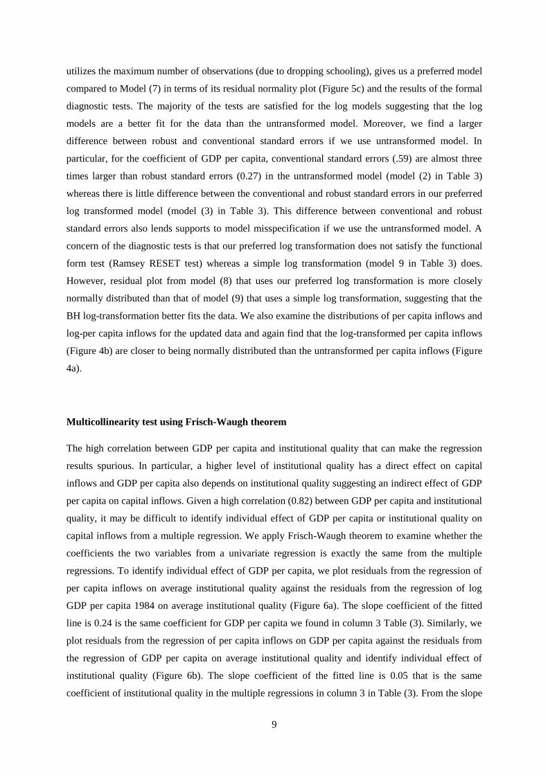
9

utilizes the maximum number of observations (due to dropping schooling), gives us a preferred model

compared to Model (7) in terms of its residual normality plot (Figure 5c) and the results of the formal

diagnostic tests. The majority of the tests are satisfied for the log models suggesting that the log

models are a better fit for the data than the untransformed model. Moreover, we find a larger

difference between robust and conventional standard errors if we use untransformed model. In

particular, for the coefficient of GDP per capita, conventional standard errors (.59) are almost three

times larger than robust standard errors (0.27) in the untransformed model (model (2) in Table 3)

whereas there is little difference between the conventional and robust standard errors in our preferred

log transformed model (model (3) in Table 3). This difference between conventional and robust

standard errors also lends supports to model misspecification if we use the untransformed model. A

concern of the diagnostic tests is that our preferred log transformation does not satisfy the functional

form test (Ramsey RESET test) whereas a simple log transformation (model 9 in Table 3) does.

However, residual plot from model (8) that uses our preferred log transformation is more closely

normally distributed than that of model (9) that uses a simple log transformation, suggesting that the

BH log-transformation better fits the data. We also examine the distributions of per capita inflows and

log-per capita inflows for the updated data and again find that the log-transformed per capita inflows

(Figure 4b) are closer to being normally distributed than the untransformed per capita inflows (Figure

4a).

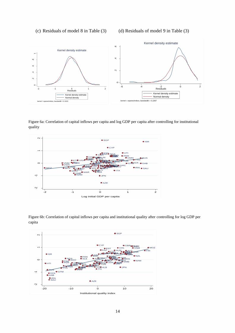
Multicollinearity test using Frisch-Waugh theorem

The high correlation between GDP per capita and institutional quality that can make the regression

results spurious. In particular, a higher level of institutional quality has a direct effect on capital

inflows and GDP per capita also depends on institutional quality suggesting an indirect effect of GDP

per capita on capital inflows. Given a high correlation (0.82) between GDP per capita and institutional

quality, it may be difficult to identify individual effect of GDP per capita or institutional quality on

capital inflows from a multiple regression. We apply Frisch-Waugh theorem to examine whether the

coefficients the two variables from a univariate regression is exactly the same from the multiple

regressions. To identify individual effect of GDP per capita, we plot residuals from the regression of

per capita inflows on average institutional quality against the residuals from the regression of log

GDP per capita 1984 on average institutional quality (Figure 6a). The slope coefficient of the fitted

line is 0.24 is the same coefficient for GDP per capita we found in column 3 Table (3). Similarly, we

plot residuals from the regression of per capita inflows on GDP per capita against the residuals from

the regression of GDP per capita on average institutional quality and identify individual effect of

institutional quality (Figure 6b). The slope coefficient of the fitted line is 0.05 that is the same

coefficient of institutional quality in the multiple regressions in column 3 in Table (3). From the slope

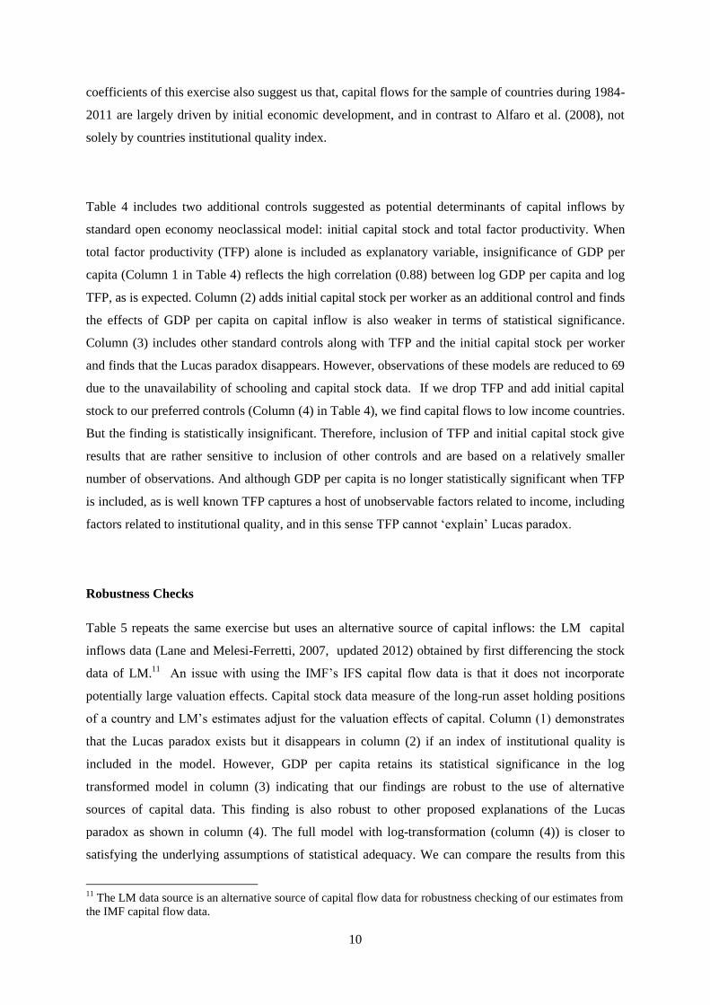
10

coefficients of this exercise also suggest us that, capital flows for the sample of countries during 1984-

2011 are largely driven by initial economic development, and in contrast to Alfaro et al. (2008), not

solely by countries institutional quality index.

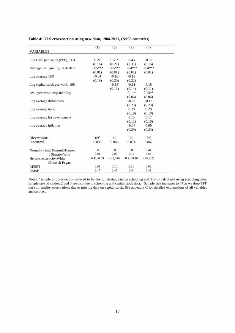
Table 4 includes two additional controls suggested as potential determinants of capital inflows by

standard open economy neoclassical model: initial capital stock and total factor productivity. When

total factor productivity (TFP) alone is included as explanatory variable, insignificance of GDP per

capita (Column 1 in Table 4) reflects the high correlation (0.88) between log GDP per capita and log

TFP, as is expected. Column (2) adds initial capital stock per worker as an additional control and finds

the effects of GDP per capita on capital inflow is also weaker in terms of statistical significance.

Column (3) includes other standard controls along with TFP and the initial capital stock per worker

and finds that the Lucas paradox disappears. However, observations of these models are reduced to 69

due to the unavailability of schooling and capital stock data. If we drop TFP and add initial capital

stock to our preferred controls (Column (4) in Table 4), we find capital flows to low income countries.

But the finding is statistically insignificant. Therefore, inclusion of TFP and initial capital stock give

results that are rather sensitive to inclusion of other controls and are based on a relatively smaller

number of observations. And although GDP per capita is no longer statistically significant when TFP

is included, as is well known TFP captures a host of unobservable factors related to income, including

factors related to institutional quality, and in this sense TFP cannot ‘explain’ Lucas paradox.

Robustness Checks

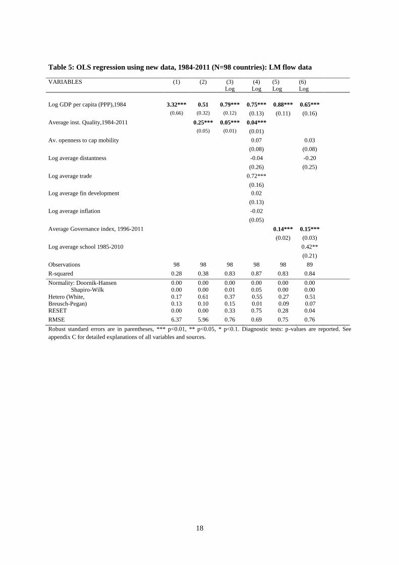
Table 5 repeats the same exercise but uses an alternative source of capital inflows: the LM capital

inflows data (Lane and Melesi-Ferretti, 2007, updated 2012) obtained by first differencing the stock

data of LM.11

An issue with using the IMF’s IFS capital flow data is that it does not incorporate

potentially large valuation effects. Capital stock data measure of the long-run asset holding positions

of a country and LM’s estimates adjust for the valuation effects of capital. Column (1) demonstrates

that the Lucas paradox exists but it disappears in column (2) if an index of institutional quality is

included in the model. However, GDP per capita retains its statistical significance in the log

transformed model in column (3) indicating that our findings are robust to the use of alternative

sources of capital data. This finding is also robust to other proposed explanations of the Lucas

paradox as shown in column (4). The full model with log-transformation (column (4)) is closer to

satisfying the underlying assumptions of statistical adequacy. We can compare the results from this

11

The LM data source is an alternative source of capital flow data for robustness checking of our estimates from

the IMF capital flow data.

11

table to AD’s findings; for example, we run models (5) and (6) similar to AD’s model (5’) and (6’) of

their Table (4). Our findings also support their claim that the index of institutional quality cannot

solve the Lucas paradox.

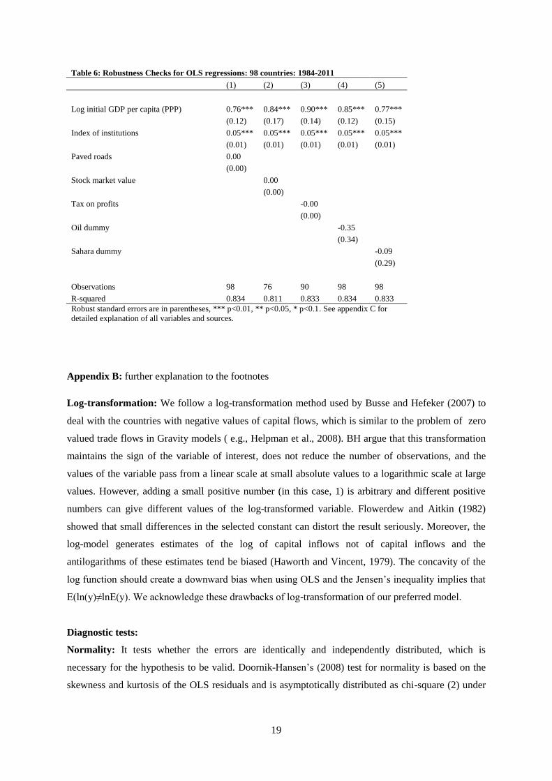
Table 6 adds extra controls that are commonly used in this literature to for the robustness checks.

Column (1) investigates the effects of infrastructure measured by percentage of paved roads in total

roads and finds a positive effect of this variable but insignificant.12

We also examine the effects of

capital market development and use stock market value over GDP.13

Column (2) finds that market

capitalization has an insignificant positive effect on capital inflows. We examine whether the tax

heaven have significant effects on capital inflows and find that, taxes on profits, income and capital

gains are negatively associated with capital inflows but again statistically insignificant.14

Column (4)

and (5) include an oil country dummy and a sub-Sahara country dummy but they also turns out as

insignificant determinants of capital inflows. A note of this robustness checks is that, we do not see

any change in terms of statistical significance and/or sing of our main variable of interests, GDP per

capita and institutional quality index.

Section V

Conclusion

We observe that existing literature that identifies specific determinant of capital inflows and argue for

a definitive explanation of the lack of capital flows from rich to poor countries however, the overall

picture of this existing literature is inconclusive. We find a conclusive answer that, the mystery of the

Lucas paradox still persists; specifically there is no single determinant that can fully capture the

positive effects of economic development on capital inflows. In other words, we find initial economic

development (i.e. initial GDP per capita) is the main driving force of capital inflows. We do not argue

that institutional qualities are not important determinants; rather we argue that an index of institutions

is not magic bullet solutions to the Lucas paradox. We confirm that our findings are based on the

better fitting models and satisfy a standard set of diagnostic tests that is surprisingly missing in the

existing literature. Moreover, our findings are based on the analysis of sample period covering more

recent data and robust to alternative sources of capital flow data.

Appendix A: Graphs and Tables

12

Alfaro et al. (2008) finds a positive but insignificant effect of infrastructure, measured by paved roads, on

capital inflows. 13

King and Levine (1993) argue that financial intermediation and financial development aid the efficient

allocation of global capital. 14

Gastanga et al (1998), Wei (2000) use tax rate as a determinant of FDI.

12

Figure 1: Histogram plots of the dependent variable (capital inflows): 1970-200015

(a) Untransformed model (b) Log-transformed model

Figure 2: Kernel density and normal density of estimated residuals: 1970-2000

(a) Residuals of Alfaro et al.’s model (b) Residuals of Alfaro et al.’s model excluding outliers

(c): Residuals of log-model including outliers (d) Residuals of log-model excluding outliers

15

Alfaro et al.’s (2008) original data set.

0

.00

2.0

04

.00

6.0

08

Den

sity

0 200 400 600 800Average Inflows of Capital per capita, 70-00, IMF

0

.05

.1.1

5.2

Den

sity

0 2 4 6 8Log average inflows per capita, 70-00, IMF

0.1

.2.3

.4.5

Den

sity

-4 -2 0 2 4Residuals

Kernel density estimate

Normal density

kernel = epanechnikov, bandwidth = 0.2651


0.2

.4.6

.8

Den

sity

-2 0 2 4 6Residuals


Normal density



0.1

.2.3

.4.5

Den

sity

-6 -4 -2 0 2 4Residuals


Normal density



0.2

.4.6

Den

sity



Normal density



13

Figure 3: Heteroscedasticity of residuals: 1970-2000

(a) Plot of residuals for Alfaro et al.’s model (b) Plot of residual for the log model

Figure 4: Histogram plots of the dependent variable (capital inflows): 1984-2011

(a) Untransformed model (b) Log-transformed model

Figure 5: Kernel density and normal density of estimated residuals

(a) Residuals of model 2 in Table (3) (b) Residuals of model 3 in Table (3)

-400

-200

0

200

400

Resi

du

als

-100 0 100 200 300Fitted values

-4-2

02

4

Resi

du

als

1 2 3 4 5 6Fitted values

0

.05

.1.1

5.2

Den

sity

0 10 20 30 40Average flow of capital per capita:1984-2011

0.2

.4.6

Den

sity

-1 0 1 2 3 4Log average flow of capital per capita:1984-2011

0

.05

.1.1

5.2

Den

sity

-10 0 10 20 30Residuals


Normal density



0.2

.4.6

.8

Den

sity



Normal density



14

(c) Residuals of model 8 in Table (3) (d) Residuals of model 9 in Table (3)

Figure 6a: Correlation of capital inflows per capita and log GDP per capita after controlling for institutional

quality

Figure 6b: Correlation of capital inflows per capita and institutional quality after controlling for log GDP per

capita

0.2

.4.6

.81

Den

sity



Normal density



0.2

.4.6

Den

sity

-6 -4 -2 0 2Residuals


Normal density



AGO

ALB

ARG

ARM AUSAUT

AZE

BFA

BGD

BGR

BLR

BOL

BRA

CAN

CHL

CIV CMR

COGCOL

CRI

CYP

CZE

DEU

DNKDOM

DZA

ECUEGY

ESP

EST

ETH

FIN

FRA

GAB

GBR

GHA

GIN

GMB

GRCGTM

GUY

HNDHRV

HTI

HUN

IDN

INDIRN

ISR

ITA

JAM

JOR

JPN

KAZ

KEN KOR

LTU

LVA

MARMDG

MEX

MLI

MOZ

MYS

NAM

NER

NGA

NIC

NLD

NOR

NZL

OMN

PAKPAN PER

PHLPNG

PRT

PRY

RUS

SAUSEN

SGP

SLE

SLVSVN

SWE

TTO

TUN

TURUGA

UKRURY

USAVNM

ZAFZMB

ZWE

-2-1

01

2

Inflo

ws

per c

apita

-2 -1 0 1 2

Log initial GDP per capita

AGO

ALB

ARG

ARMAUS

AUT

AZE

BFABGD BGR

BLR

BOL BRA

CAN

CHL

CIV

CMRCOG

COL CRI

CYP

CZE

DEU

DNK

DOM

DZA

ECU

EGY

ESP

EST

ETHFIN

FRA

GAB

GBR

GHA

GIN

GMB

GRC

GTM

GUYHND

HRV

HTI

HUN

IDN

IND

IRN

ISR

ITA

JAM

JOR

JPN

KAZ

KEN

KORLTU

LVA

MAR

MDG

MEX

MLI

MOZ

MYS

NAM

NER

NGA

NIC

NLD

NOR

NZL

OMNPAK

PAN

PER

PHL

PNG

PRT

PRYRUS

SAU

SEN

SGP

SLE

SLV

SVN

SWE

TTO

TUN

TUR

UGA

UKR

URY

USA

VNM

ZAF

ZMB

ZWE

-2-1

01

2

Inflo

ws

per c

apita

-20 -10 0 10 20

Institutional quality index

15

Table 1: Replication of Alfaro et al.’s Table 3, 1970-2000 (N=98 countries)

(1) (2) (2*) (2’) (2**) (3) (4) (4*) (5) (6) (7) (7*) VARIABLES Whole

World

Whole

World

Whole

World

Whole

World

Whole

World

Base

Sample

Base

Sample

Base

Sample

Base

Sample

Base

Sample

Base

Sample

Base

Sample

Log GDP pc (PPP) 1970

1.05***

(0.17) 0.20

(0.13) 0.69**

(0.27) 0.24**

(0.11) 0.97***

(0.18) 1.18***

(0.19 0.14

(0.20) 0.85***

(0.22)

Log av GDP pc

(PPP) 0.84

(0.13) 0.20

(0.13)

0.49**

(.23)

Av institutional

quality,1984-2000

0.68*** 0.51*** 0.49*** 0.47*** 0.75*** 0.51***

0.82*** 0.67*** 0.47**

(0.14) (0.18) (0.10) (0.10) ((0.17) (0.12) (0.12) (0.15) (.23)

R-squared 0.37 0.52 0.47 0.54 0.78 0.39 0.52 0.81 0.52 0.44 0.53 0.46

Observations 98 98 98 93 90 81 81 73 81 81 81 81

Normality test:

Doornik-Hansen

Shapiro-Wilk

0.00 0.00

0.00 0.00

0.00 0.00

0.00 0.00

0.64 0.28

0.00 0.00

0.00 0.00

0.50 0.11

0.00 0.00

0.00 0.00

0.00 0.00

0.00 0.00

Heteroscedasticity:

White

Breusch-Pegan

0.00

0.00

0.00

0.00

0.74

0.36

0.00

0.00

0.17

0.02

0.00

0.00

0.00

0.00

0.18

0.16

0.00

0.00

0.00

0.00

0.00

0.00

0.77

0.36

RESET 0.00 0.00 0.62 0.00 0.08 0.00 0.00 0.03 0.00 0.00 0.00 0.73

RMSE 1.26 1.11 1.39 0.76 0.78 1.33 1.19 0.74 1.18 1.70 1.18 1.44

Notes: 2* and 7* use log (per capital inflows) as dependent variables, 2** uses log (per capita inflows) as dependent

variable and removes outliers, 2’ uses per capita inflows as dependent variable and removes outliers, and the other remaining

models use per capital inflows as dependent variable. Robust standard errors are in parentheses, *** p<0.01, ** p<0.05, *

p<0.1. Diagnostic tests: p-values are reported. See appendix C for detailed explanations of all variables and sources.

Table 2: Replication of Alfaro et al.’s Table 4, 1970-2000 (N=98 countries)

(1) (2) (3) (4) (5) (6) (7) (7*) (8) (8*)

VARIABLES Whole

World

Whole

World

Whole

World

Base

Sample

Base

Sample

Base

Sample

Base

Sample

Base

Sample

Base

Sample

Base

Sample

Log GDP pc (PPP) 1970 1.12*** 0.99*** 0.82*** 1.14*** 1.11*** 0.91*** 0.13 0.56**

Log GDP pc ($1996) 1970

(0.24)

(0.17) (0.14) (0.24) (0.19) (0.16) (0.19)

(0.23)

0.21 (0.16)

0.47*** (0.16)

Av institutional quality,1984-2000 0.65*** 0.48*** 0.59*** 0.43***

(0.16) (0.11) (0.14) (0.12)

Log average school 1970-2000 0.09 0.06 -0.10 0.47** -0.19 0.40**

(0.18) (0.18) (0.15) (0.16) (0.20)

(0.17)

Log average distantness -0.68 -0.58 -0.29 0.50* -0.28 0.48

(0.71) (0.73) (0.60) (0.30) (0.60) (0.30)

Average restrictions to capital

mobility

-1.54***

(0.53)

-1.83***

(0.61)

-1.23**

(0.48)

-0.62

(0.41)

-1.18**

(0.46)

-0.60

(0.37)

R-squared 0.39 0.38 0.42 0.39 0.39 0.45 0.54 0.83 0.55 0.84

Observations 82 97 97 81 81 81 81 73 81 73

Normality test: Doornik-Hansen

: Shapiro-Wilk

0.00

0.00

0.00

0.00

0.00

0.00

0.00

0.00

0.00

0.00

0.00

0.00

0.00

0.00

0.61

0.62

0.00

0.00

0.34

0.33

Heteroscedasticity: White’s

Breusch-Pegan

0.00 0.00

0.00 0.00

0.00 0.00

0.00 0.00

0.00 0.00

0.00 0.00

0.01 0.00

0.05 0.29

0.01 0.00

0.15 0.42

RESET 0.00 0.00 0.00 0.00 0.00 0.00 0.00 0.31 0.00 0.23

RMSE 1.34 1.26 1.22 1.34 1.33 1.27 1.18 0.69 1.28 0.67

16

Note: 7* and 8* are the log-transformed model and excluding outliers. Robust standard errors are in parentheses, ***

p<0.01, ** p<0.05, * p<0.1. Diagnostic tests: p-values are reported. See appendix C for detailed explanations of all variables

and sources.

Table 3: OLS cross-section using new data, 1984-2011 (N=98 countries)

(1) (2) (3) (4) (5) (6) (7) (8) (9)

VARIABLES Linear Linear Log Linear Log Log Log Log Log

Log GDP pc (PPP) 1984 2.58*** 0.30 0.24*** 0.37* 0.27*** 0.18** 0.20** 0.18*** 0.64***

(0.44) (0.27) (0.07) (0.20) (0.05) (0.09) (0.11) (0.07) (0.21)

Av inst quality,1984-2011 0.20*** 0.05*** 0.04*** 0.04*** 0.04*** 0.06***

(0.04) (0.01) (0.01) (0.01) (0.01)

(0.02)

Average governance

index,1996-2011

0.65***

(0.12)

0.14***

(0.01)

Average open to cap mobility 0.09 0.08 0.09* 0.03

(0.05) (0.05) (0.05) (0.10)

Log average school 1985-2010 0.07 0.01

(0.14) (0.16)

Log average distantness -0.22 -0.20 -0.20 0.25

(0.20) (0.21) (0.20) (0.32)

Log average trade 0.19 0.18 0.72***

(0.17) (0.16) (0.21)

Log average fin development 0.14 0.18* 0.02

(0.09) (0.10) (0.16)

Log average inflation 0.03 0.03 -0.43***

(0.05) (0.04)

(0.10)

Observations 98 98 98 98 98 89 89 98 97

R-squared 0.34 0.46 0.81 0.51 0.84 0.83 0.84 0.83 0.80


: Shapiro-Wilk

0.00

0.00

0.00

0.00

0.00

0.01

0.00

0.00

0.00

0.00

0.00

0.00

0.11

0.32

0.13

0.39

0.00

0.00

Heteroscedasticity:White

:Breusch-Pegan

0.11 0 .09

0.56 0.08

0.67 0.21

0.42 0.04

0.81 0.40

0.03 0.10

0.01 0.10

0.02 0.23

0.46 0.22

RESET 0.00 0.00 0.00 0.00 0.00 0.01 0.00 0.00 0.80

RMSE 4.34 3.92 0.50 3.74 0.44 0.47 0.46 0.48 0.92

Notes: Alfaro’s whole world (98) country sample is used. Dependent variable is average capital inflows per capita for

Models (1, 2, and 4) as used in Alfaro et al. (2008). Dependent variable is log of the average capital inflows per capita in

models (3, 5, 6, 7, 8, and 9). Robust standard errors are in parentheses, *** p<0.01, ** p<0.05, * p<0.1 Diagnostic tests: p-

values are reported for each corresponding test. See appendix C for detailed explanations of all variables and sources.

17

Table 4: OLS cross-section using new data, 1984-2011, (N=98 countries)

(1) (2) (3) (4)

VARIABLES

Log GDP per capita (PPP),1984 0.21 0.51* 0.43 -0.09

(0.16) (0.27) (0.31) (0.16)

Average inst. quality,1984-2011 0.05*** 0.05*** 0.04*** 0.04***

(0.01) (0.01) (0.01) (0.01)

Log average TFP -0.04 -0.16 -0.18

(0.18) (0.20) (0.22)

Log capital stock per work, 1984 -0.18 -0.11 0.18

(0.11) (0.14) (0.11)

Av. openness to cap mobility 0.11* 0.13**

(0.06) (0.06)

Log average distantness -0.20 -0.13

(0.25) (0.23)

Log average trade 0.28 0.28

(0.19) (0.18)

Log average fin development 0.15 0.17

(0.11) (0.10)

Log average inflation -0.04 0.06

(0.29) (0.25)

Observations 69a 69 69 74b

R-squared 0.839 0.843 0.874 0.867


: Shapiro-Wilk

0.00

0.01

0.00

0.00

0.09

0.16

0.44

0.65

Heteroscedasticity:White

:Breusch-Pegan

0.41, 0.09 0.43,0.09 0.21, 0.10 0.07,0.22

RESET 0.09 0.10 0.01 0.00

RMSE 0.47 0.47 0.44 0.45

Notes: a sample of observations reduced to 69 due to missing data on schooling and TFP is calculated using schooling data,

sample size of models 2 and 3 are also due to schooling and capital stock data, b Sample size increases to 74 as we drop TFP

but still smaller observations due to missing data on capital stock. See appendix C for detailed explanations of all variables

and sources.

18

Table 5: OLS regression using new data, 1984-2011 (N=98 countries): LM flow data

VARIABLES (1) (2) (3)

Log

(4)

Log

(5)

Log

(6)

Log

Log GDP per capita (PPP),1984 3.32*** 0.51 0.79*** 0.75*** 0.88*** 0.65***

(0.66) (0.32) (0.12) (0.13) (0.11) (0.16)

Average inst. Quality,1984-2011 0.25*** 0.05*** 0.04***

(0.05) (0.01) (0.01)

Av. openness to cap mobility 0.07 0.03

(0.08) (0.08)

Log average distantness -0.04 -0.20

(0.26) (0.25)

Log average trade 0.72***

(0.16)

Log average fin development 0.02

(0.13)

Log average inflation -0.02

(0.05)

Average Governance index, 1996-2011 0.14*** 0.15***

(0.02) (0.03)

Log average school 1985-2010 0.42**

(0.21)

Observations 98 98 98 98 98 89

R-squared 0.28 0.38 0.83 0.87 0.83 0.84

Normality: Doornik-Hansen

Shapiro-Wilk

0.00

0.00

0.00

0.00

0.00

0.01

0.00

0.05

0.00

0.00

0.00

0.00

Hetero (White,

Breusch-Pegan)

0.17

0.13

0.61

0.10

0.37

0.15

0.55

0.01

0.27

0.09

0.51

0.07

RESET 0.00 0.00 0.33 0.75 0.28 0.04

RMSE 6.37 5.96 0.76 0.69 0.75 0.76

Robust standard errors are in parentheses, *** p<0.01, ** p<0.05, * p<0.1. Diagnostic tests: p-values are reported. See

appendix C for detailed explanations of all variables and sources.

19

Table 6: Robustness Checks for OLS regressions: 98 countries: 1984-2011

(1) (2) (3) (4) (5)

Log initial GDP per capita (PPP) 0.76*** 0.84*** 0.90*** 0.85*** 0.77***

(0.12) (0.17) (0.14) (0.12) (0.15)

Index of institutions 0.05*** 0.05*** 0.05*** 0.05*** 0.05***

(0.01) (0.01) (0.01) (0.01) (0.01)

Paved roads 0.00

(0.00)

Stock market value 0.00

(0.00)

Tax on profits -0.00

(0.00)

Oil dummy -0.35

(0.34)

Sahara dummy -0.09

(0.29)

Observations 98 76 90 98 98

R-squared 0.834 0.811 0.833 0.834 0.833

Robust standard errors are in parentheses, *** p<0.01, ** p<0.05, * p<0.1. See appendix C for

detailed explanation of all variables and sources.

Appendix B: further explanation to the footnotes

Log-transformation: We follow a log-transformation method used by Busse and Hefeker (2007) to

deal with the countries with negative values of capital flows, which is similar to the problem of zero

valued trade flows in Gravity models ( e.g., Helpman et al., 2008). BH argue that this transformation

maintains the sign of the variable of interest, does not reduce the number of observations, and the

values of the variable pass from a linear scale at small absolute values to a logarithmic scale at large

values. However, adding a small positive number (in this case, 1) is arbitrary and different positive

numbers can give different values of the log-transformed variable. Flowerdew and Aitkin (1982)

showed that small differences in the selected constant can distort the result seriously. Moreover, the

log-model generates estimates of the log of capital inflows not of capital inflows and the

antilogarithms of these estimates tend be biased (Haworth and Vincent, 1979). The concavity of the

log function should create a downward bias when using OLS and the Jensen’s inequality implies that

E(ln(y)≠lnE(y). We acknowledge these drawbacks of log-transformation of our preferred model.

Diagnostic tests:

Normality: It tests whether the errors are identically and independently distributed, which is

necessary for the hypothesis to be valid. Doornik-Hansen’s (2008) test for normality is based on the

skewness and kurtosis of the OLS residuals and is asymptotically distributed as chi-square (2) under

20

the null of normality. We also use Shapiro-Wilk W test where the p-value is based on the assumption

that the distribution is normal.

Homoscedasticity: Homoscedastic errors is one of the main assumptions of OLS regression. If the

model is well fitted, there should not be any pattern to the residuals plotted against the fitted values.

We employ two tests for homoscedasticity: the Breusch-Pegan (1980) test and the White’s test (a

special case of Breusch-Pegan test). P-value of the null hypothesis is based on the assumption that the

variance of the residuals is homogenous.

Functional form: A model specification error can occur when one or more relevant variables are

omitted or one or more irrelevant variables are included in the model. We use Ramsey RESET test

(Stata’s ovtest) that creates new variables based on the predictors and refits the model using those new

variables to see if any of them would be significant. The p-value of the null hypothesis is based on the

assumption that the model has no omitted variables.

RMSE (root mean square error): RMSE is frequently used as a measure of the difference between

values predicted by a model or an estimator and the values actually observed. In other words, it is the

standard deviation of the errors and measures the spread of the data around the regression line. The

smaller the value of RMSE, the better the fitted line in terms of prediction.

Appendix C: Data descriptions and sources

Capital inflows per capita, 1984-2011: Sum of FDI (IFS line: BFDIA) and portfolio (IFS line: BFPLE)

inflows (2013). The data is in current US dollars are deflated by US CPI

with base year 2005=1 and divided by population.

Stocks of foreign capital (LM), 1984-2011: Foreign claims on domestic capital, from Lane and Milesi-Ferretti

(2012). Capital inflows are obtained by the first difference of stock data of

LM.

GDP per capita in 1984 in PPP dollars: GDP at PPP from Penn World Tables, Ver. 7.1, Heston, Summers,

and Aten (2012), divided by population.

GDP per capita, 1984-2011 in constant 2005 dollars: GDP from WDI, World Bank (2012), divided by

population.

Institutional Quality, 1984-2011: This is a composite index, which is the sum of yearly rating of the 12

components from International Country Risk Guide, the PRS Group (2012).

To ensure the consistency of interpretation, each component of the index is

rescaled, as follows, to range from 0 to 10. Thus, the theoretical range of

this index is 0 to 120, where a higher score means institutional qualities are

better and lower risks.

Governance Indicator, 1996-2011: Alternative measures of an institutions index. Composite indicator is the

average of yearly rating of 5 indicators. Data are taken from Kaufmann et

al., (2010, updated 2013).

Openness to capital mobility, 1984-2011: Measures a country’s degree of capital account openness based on

the IMF’s Annual Report on Exchange Arrangements and Exchange

Restrictions developed by Chinn and Ito (2006, 2012), where a higher index

value indicates greater capital account openness. Values range from

21

2.6(most financially open) to -2.6 (least financially open). Unlike ours, for

restrictions on capital mobility Alfaro et al. (2008) use the mean value of

four dummy variables from IMF’s Annual Report on Exchange

Arrangements and Exchange Restrictions: exchange arrangements;

payments restrictions for capital transactions, payments restrictions on

payment for capital transactions; and surrender or repatriation requirements

for export proceeds.

Schooling, 1985-2010 : Years of schooling of persons of age 25 or above is a measure of stock of

human capital (h) at five-year intervals. Linear interpolation is used to fill in

the missing date between the 5-yearly observations. Source: Barro and Lee

(1996, updated 2010).

Financial Development, 1984-2011: Domestic credit to the private sector (% of GDP), data are taken from

Beck et al. (2012).

Trade, 1984-2011 : Sum of exports and imports (% of GDP), data are taken from WDI, World

Bank (2013).

Distantness : Population weighted distance from the capital city of a country to capital

cities of other countries, data are taken from CEPII (2013).

Inflation, 1984-2011 : Consumer prices (annual %), data are taken from WDI, World Bank

References

Abiad, A., Leigh, D., & Mody, A. (2009). Financial integration, capital mobility, and income convergence.

Economic Policy, 24(58), 241-305.

Alfaro, L., Kalemli-Ozcan, S., & Volosovych, V. (2008). Why Doesn't Capital Flow from Rich to Poor

Countries? An Empirical Investigation. The Review of Economics and Statistics, 90(2), 347-368.

Azémar, C., & Desbordes, R. (2013). Has the Lucas Paradox been fully explained? Economics Letters, 121(2),

183-187.

Barro, R. J., & Lee, J.-W. (2012). A new data set of educational attainment in the world, 1950–2010. Journal of

Development Economics.

Breusch, T. S., & Pagan, A. R. (1980). The Lagrange multiplier test and its applications to model specification

in econometrics. Review of Economic Studies, 239-253.

Busse, M., & Hefeker, C. (2007). Political risk, institutions and foreign direct investment. European Journal of

Political Economy, 23(2), 397-415.

Clemens, M. A., & Williamson, J. G. (2004). Wealth bias in the first global capital market boom, 1870–1913*.

Economic Journal, 114(495), 304-337.

Doornik, J. A., & Hansen, H. (2008). An omnibus test for univariate and multivariate normality*. Oxford

Bulletin of Economics and Statistics, 70(s1), 927-939.

Flowerdew, R., & Aitkin, M. (1982). A method of fitting the gravity model based on the Poisson distribution.

Journal of Regional Science, 22(2), 191-202.

Forbes, K. J. (2010). Why do foreigners invest in the United States? Journal of International Economics, 80(1),

3-21.

Gastanaga, V. M., Nugent, J. B., & Pashamova, B. (1998). Host country reforms and FDI inflows: How much

difference do they make? World Development, 26(7), 1299-1314.

Gourinchas, P.-O., & Jeanne, O. (2013). Capital flows to developing countries: The allocation puzzle. Review of

Economic Studies.

Hashimoto, Y., & Wacker, K. M. (2012). The Role of Risk and Information for International Capital Flows:

New Evidence from the SDDS: IMF working paper, wp/12/242

Haworth, J., & Vincent, P. (1979). The stochastic disturbance specification and its implications for log-linear

regression. Environment and Planning A, 11(7), 781-790.

Helpman, E., Melitz, M., & Rubinstein, Y. (2008). Estimating trade flows: Trading partners and trading

volumes. Quarterly Journal of Economics, 123(2), 441-487.

Henry, P. B. (2007). Capital Account Liberalization: Theory, Evidence, and Speculation. Journal of Economic

22

Literature, 45, 887-935.

International Monetary Fund, International Financial Statistics, Online data retrieved on March 30, 2013,

Washington, DC: International Monetary Fund.

Kalemli-Ozcan, S., Reshef, A., Sørensen, B. E., & Yosha, O. (2010). Why does capital flow to rich states?

Review of Economics and Statistics, 92(4), 769-783.

Kaufmann, D., Kraay, A., & Mastruzzi, M. (2010). The worldwide governance indicators: methodology and

analytical issues. World Bank Policy Research Working Paper (5430).

King, G., & Roberts, M. (2012). How Robust Standard Errors Expose Methodological Problems They Do Not

Fix. Paper presented at the Annual Meeting of the Society for Political Methodology, Duke University.

King, R. G., & Levine, R. (1993). Finance and growth: Schumpeter might be right. Quarterly Journal of

Economics, 108(3), 717-737.

Lane, P. R., & Milesi-Ferretti, G. M. (2007). The external wealth of nations mark II: Revised and extended

estimates of foreign assets and liabilities, 1970–2004. Journal of International Economics, 73(2), 223-

250.

Lucas, R. E. (1990). Why doesn't capital flow from rich to poor countries? American Economic Review, 80(2),

92-96.

Mayer, T., & Zignago, S. (2011). Notes on CEPII’s distances measures: The GeoDist database.

Mody, A., Taylor, M. P., & Kim, J. Y. (2001). Modelling fundamentals for forecasting capital flows to

emerging markets. International Journal of Finance & Economics, 6(3), 201-216.

Okada, K. (2012). The Interaction Effects of Financial Openness and Institutions on International Capital Flows.

Journal of Macroeconomics.

Papaioannou, E. (2009). What drives international financial flows? Politics, institutions and other determinants.

Journal of Development Economics, 88(2), 269-281.

Portes, R., & Rey, H. (2005). The determinants of cross-border equity flows. Journal of International

Economics, 65(2), 269-296.

PRS Group, International Country Risk Guide (New York: PRS group 2013)

Reinhardt, D., Ricci, L. A., & Tressel, T. (2013). International capital flows and development: Financial

openness matters. Journal of International Economics, 91(2), 235-251.

Reinhart, C. M., & Rogoff, K. S. (2004). Serial default and the" paradox" of rich to poor capital flows.

American Economic Review, 94(2), 53-58.

Solow, R. M. (1956). A contribution to the theory of economic growth. Quarterly Journal of Economics, 70(1),

65-94.

Verardi, V. & Croux C. (2009). Robust regression in stata, Stata Journal 9(3), 439-453.

Von Hagen, J., & Zhang, H. (2010). Financial development and the patterns of international capital flows.

Working paper (02/2010), Singapore Management University.

Wei, S. J. (2000). How taxing is corruption on international investors? Review of Economics and Statistics,

82(1), 1-11.

World Bank, World Development Indicators, online data retrieved March 30, 2013, Washington,DC World

Bank, 2013.

Documents

Determinants of Capital Inflows: New Empirical Evidence … · 2017-11-30 · 1 Determinants of Capital Inflows: New Empirical Evidence Introduction The simplest benchmark neoclassical