Design Synthesis of Articulated Heavy Vehicles With Active Trailer Steering Systems

Design Synthesis of Articulated

Heavy Vehicles with Active Trailer

Steering Systems

by

Md. Manjurul Islam

A thesis

presented to the University of Ontario Institute of Technology

in fulfillment of the

thesis requirement for the degree of

Master of Applied Science

in

Automotive Engineering

Oshawa, Ontario, Canada, 2010

©Md. Manjurul Islam 2010

ii

iii

AUTHOR'S DECLARATION

I hereby declare that I am the sole author of this thesis. This is a true copy of the thesis,

including any required final revisions, as accepted by my examiners.

I understand that my thesis may be made electronically available to the public.

iv

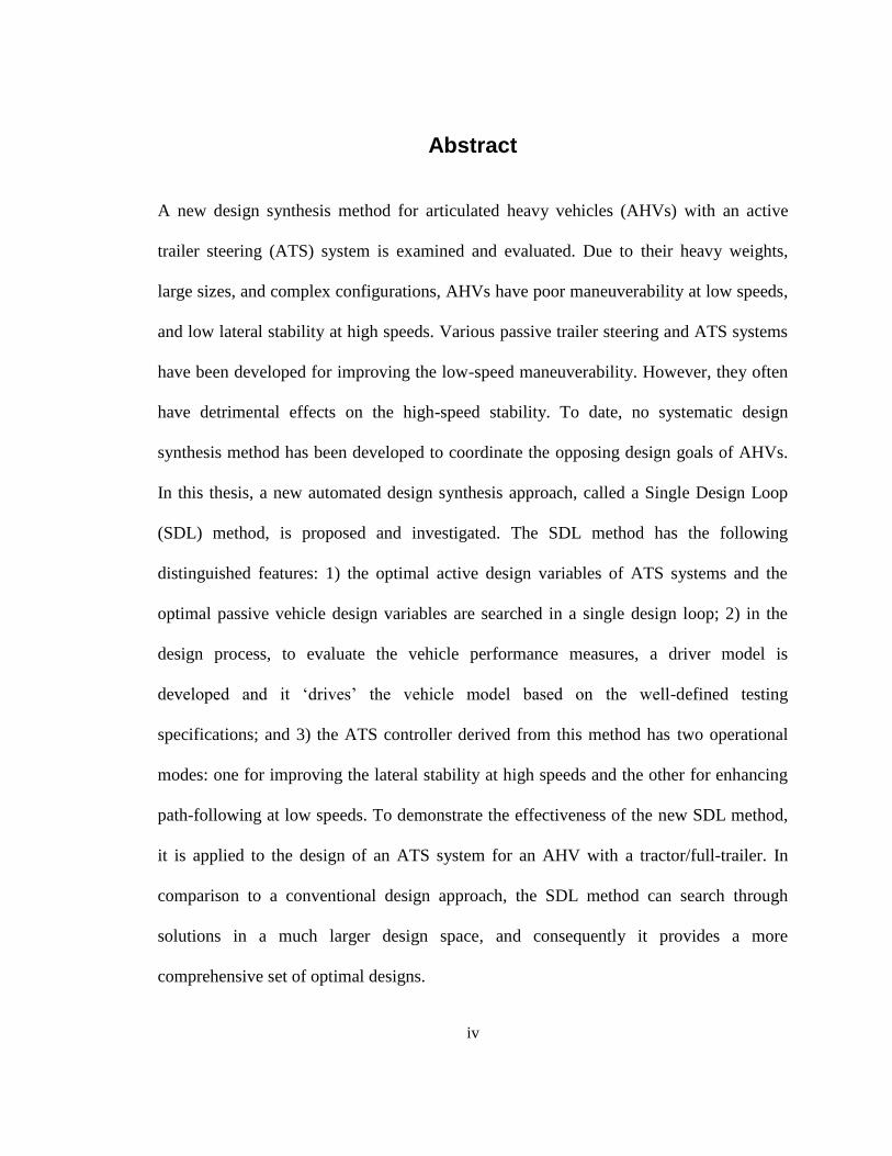
Abstract

A new design synthesis method for articulated heavy vehicles (AHVs) with an active

trailer steering (ATS) system is examined and evaluated. Due to their heavy weights,

large sizes, and complex configurations, AHVs have poor maneuverability at low speeds,

and low lateral stability at high speeds. Various passive trailer steering and ATS systems

have been developed for improving the low-speed maneuverability. However, they often

have detrimental effects on the high-speed stability. To date, no systematic design

synthesis method has been developed to coordinate the opposing design goals of AHVs.

In this thesis, a new automated design synthesis approach, called a Single Design Loop

(SDL) method, is proposed and investigated. The SDL method has the following

distinguished features: 1) the optimal active design variables of ATS systems and the

optimal passive vehicle design variables are searched in a single design loop; 2) in the

design process, to evaluate the vehicle performance measures, a driver model is

developed and it „drives‟ the vehicle model based on the well-defined testing

specifications; and 3) the ATS controller derived from this method has two operational

modes: one for improving the lateral stability at high speeds and the other for enhancing

path-following at low speeds. To demonstrate the effectiveness of the new SDL method,

it is applied to the design of an ATS system for an AHV with a tractor/full-trailer. In

comparison to a conventional design approach, the SDL method can search through

solutions in a much larger design space, and consequently it provides a more

comprehensive set of optimal designs.

v

Acknowledgements

I would like to thank my supervisor Dr. Yuping He for his encouragement, support and

guidance during my thesis work. I would also like to thank my supervisory committee

members Dr. Ghaus Rizvi and Dr. Hossam Kishawy for serving on my thesis committee

and making significant contribution to enhance the quality of this work. Financial support

of this research by the Natural Science and Engineering Research Council of Canada and

Genist Systems Company is gratefully acknowledged.

vi

Dedication

I would like to thank also my mom and dad for their unconditional love, affection and

support in my life.

vii

Table of Contents

AUTHOR'S DECLARATION........................................................................................................ iii

Abstract ........................................................................................................................................... iv

Acknowledgements .......................................................................................................................... v

Dedication ....................................................................................................................................... vi

Table of Contents ........................................................................................................................... vii

List of Figures .................................................................................................................................. x

List of Tables ................................................................................................................................ xiii

Nomenclature ................................................................................................................................ xiv

Chapter 1 INTRODUCTION ........................................................................................................... 1

1.1 WHY ARE ARTICULATED HEAVY VEHICLES WIDELY USED? ............................... 1

1.2 VEHICLE CONFIGURATIONS .......................................................................................... 1

1.3 MOTIVATION ...................................................................................................................... 2

1.4 THESIS CONTRIBUTIONS ................................................................................................. 8

1.5 THESIS ORGANIZATION ................................................................................................... 9

Chapter 2 LITERATURE REVIEW .............................................................................................. 10

2.1 INTRODUCTION ............................................................................................................... 10

2.2 PASSIVE TRAILER STEERING SYSTEMS .................................................................... 10

2.2.1 Low-Speed Maneuverability ......................................................................................... 11

2.2.2 Poor High-Speed Stability ............................................................................................ 12

2.3 ACTIVE TRAILER STEERING SYSTEMS ...................................................................... 12

2.3.1 RWA Ratio as a Control Criterion ................................................................................ 13

2.3.2 Simulation Environments .............................................................................................. 14

2.3.3 Passive and Active Steering System Together .............................................................. 15

2.4 CONTROLLER DESIGN FOR ATS SYSTEMS ............................................................... 16

2.5 LIMITATIOINS OF EXISTING DESIGN AND ANALYSIS METHODS ....................... 18

Chapter 3 VEHICLE MODELING AND DESIGN TOOLS ........................................................ 20

3.1 INTRODUCTION ............................................................................................................... 20

3.2 VEHICLE MODELING ...................................................................................................... 20

3.2.1 Model-1 ......................................................................................................................... 20

3.2.2 Model-2 ......................................................................................................................... 23

viii

3.3 TEST MENEUVERS........................................................................................................... 25

3.3.1 Open-Loop Simulation .................................................................................................. 25

3.3.2 Closed-Loop Simulation ............................................................................................... 27

3.4 LINEAR QUADRATIC REGULATOR TECHNIQUE ..................................................... 28

3.5 GENETIC ALGORITHMS ................................................................................................. 29

3.5.1 Genetic Algorithm and Optimization ............................................................................ 30

3.5.2 Genotype ....................................................................................................................... 30

3.5.3 Fitness Function ............................................................................................................ 31

3.5.4 Genetic Algorithm Operators ........................................................................................ 32

Chapter 4 TWO DESIGN LOOP METHOD FOR THE DESIGN OF AHVS WITH ATS

SYSTEM ........................................................................................................................................ 34

4.1 INTRODUCTION ............................................................................................................... 34

4.2 VEHICLE SYSTEM MODELS .......................................................................................... 35

4.2.1 Vehicle Model ............................................................................................................... 35

4.2.2 Maneuver Emulated ...................................................................................................... 35

4.3 OPTIMAL CONTROL DESIGN ........................................................................................ 36

4.4 PROPOSED TSD METHOD .............................................................................................. 37

4.4.1 Method for Determining Controller Weighting Factors ............................................... 37

4.4.2 Proposed Integrated Design Method ............................................................................. 39

4.5 RESULT AND DISCUSSION ............................................................................................ 41

4.5.1 Simulation Results of Baseline Case ............................................................................ 41

4.5.2 Simulation Results of Control Case .............................................................................. 44

4.5.3 Simulation Results of Optimal Case ............................................................................. 50

4.6 CONCLUSIONS.................................................................................................................. 55

Chapter 5 SINGLE DESIGN LOOP METHOD FOR THE DESIGN OF AHVS WITH ATS

SYSTEMS ..................................................................................................................................... 57

5.1 INTRODUCTION ............................................................................................................... 57


5.2.1 Vehicle Model ............................................................................................................... 58

5.2.2 Maneuvers emulated ..................................................................................................... 58

5.2.3 Driver Model ................................................................................................................. 59

5.2.4 LQR Controller for ATS Systems ................................................................................. 64

ix

5.3 AUTOMATED DESIGN SYNTHESIS APPROACH ........................................................ 66

5.4 RESULTS AND DISCUSSION .......................................................................................... 68

5.5 CONCLUSIONS.................................................................................................................. 78

Chapter 6 A COMPOUND LATERAL POSITION DEVIATION PREVIEW CONTROLLER . 80

6.1 INTRODUCTION ............................................................................................................... 80


6.2.1 Vehicle Model ............................................................................................................... 81

6.2.2 Maneuver Emulated ...................................................................................................... 81

6.3 CLPDP CONTROLLER DESIGN ...................................................................................... 82

6.3.1 Proposed Control Strategy ............................................................................................ 82

6.3.2 Design Criteria .............................................................................................................. 84

6.3.3 CLPDP Controller Design ............................................................................................ 85

6.4 NUMERICAL SIMULATION ............................................................................................ 87

6.5 CONCLUSIONS.................................................................................................................. 91

Chapter 7 CONCLUSIONS ........................................................................................................... 93

7.1 INTRODUCTION ............................................................................................................... 93

7.2 PROPOSED SYNTHESIS METHOD ................................................................................ 93

7.3 COMPOUND LATERAL POSITION DEVIATION PREVIEW CONTROLLER ........... 95

7.4 DIRECTIONS FOR FUTURE RESEARCH ....................................................................... 96

APPENDIX A: VEHICLE MODEL SYSTEM MATRICES .................................................. 107

APPENDIX B: VEHICLE MODEL SYSTEM PARAMETERS ............................................ 110

x

List of Figures

Fig. 1.1: Roll-over of an AHV during high-speed turning maneuver ............................................. 3

Fig. 1.2: High speed Path-Following Off-Tracking during constant radius turn maneuver ........... 6

Fig. 1.3: Low speed Path-Following Off-Tracking ......................................................................... 7

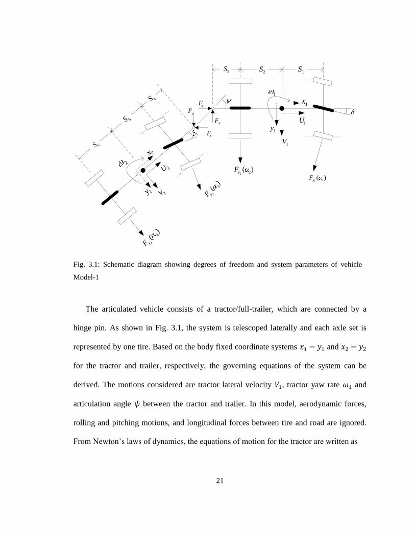
Fig. 3.1: Schematic diagram showing degrees of freedom and system parameters of vehicle

Model-1 .......................................................................................................................................... 21


Model-2 .......................................................................................................................................... 24

Fig. 3.3: (a) layout of circle path-following test course; (b) step steer input for circle path-

following [26] ................................................................................................................................ 26

Fig. 4.1: The optimization method for determining LQR controller weighting factors ................ 39

Fig. 4.2: Schematic representation of the proposed design synthesis approach ........................... 42

Fig. 4.3: Baseline case in lane change maneuver (the amplitude of sinusoid steer input, , taking

the value of 0.0113): (a) lateral accelerations at tractor and trailer CG versus time and lateral

displacement of tractor front axle centre and that of trailer rear axle center versus time; (b)

trajectory of tractor front axle center and that of trailer rear axle .................................................. 43

Fig. 4.4: Baseline case in low-speed circle path-following maneuver (with a step steer input of

): trajectory of tractor front axle centre and that of trailer rear axle centre axle

center .............................................................................................................................................. 44

Fig. 4.5: PFOT versus controller weighting factors (low-speed PFOT control mode): (a) PFOT

versus and , (b) PFOT versus and , and (c) PFOT versus and ; RWA ratio

versus weighting factors (high-speed RWA control mode): (d) RWA ratio versus and , (e)

RWA ratio versus and , and (f) RWA ratio versus and ............................................. 47

Fig. 4.6: Control case with RWA control mode in high-speed lane change maneuver (the

amplitude of the sinusoid steering input, A, taking the value of 0.0113): (a) trajectory of tractor

front axle centre and that of trailer rear axle centre; (b) lateral acceleration at CG of tractor and

trailer versus time ........................................................................................................................... 49


amplitude of the sinusoid steer input, A, taking the value of 0.09): (a) trajectory of tractor front

axle centre and that of trailer rear axle centre; (b) lateral acceleration at CG of tractor and trailer

versus time ..................................................................................................................................... 50

xi

Fig. 4.8: Optimal case in high-speed lane change maneuver (the amplitude of the sinusoid steer

input, , taking the value of 0.09): (a) lateral acceleration at CG of tractor and trailer versus time

and lateral displacement of tractor front axle centre and that of trailer rear axle centre versus time;

(b) trajectory of tractor front axle centre and that of trailer rear axle centre .................................. 54

Fig. 4.9: Optimal case in low-speed circle path-following maneuver (with a step steer input of

): trajectory of tractor front axle centre and that of trailer rear axle centre......... 55

Fig. 5.1: Geometry representation of vehicle and prescribed path ............................................... 60

Fig. 5.2: Simulated trajectory of the tractor front axle center from the high-speed single lane

change maneuver ........................................................................................................................... 64

Fig. 5.3: Simulated trajectory of the tractor front axle center from the low-speed 90-degree

intersection turn maneuver ............................................................................................................. 65

Fig. 5.4: Schematic representation of the automated design synthesis approach ......................... 69

Fig. 5.5: Lateral acceleration at CG of tractor and trailer versus time (results achieved in the

simulated high-speed lane change maneuver): (a) baseline design case; (b) SDL design case ..... 72

Fig. 5.6: Trajectory of track front axle center and that of trailer rear axle center (results achieved

in the simulated high-speed lane change maneuver): (a) baseline design case; (b) SDL design case

....................................................................................................................................................... 72

Fig. 5.7: Trajectory of tractor‟s front axle center and that of trailer‟s rear axle center (results

achieved in the simulated low-speed 90-degree intersection turn maneuver): (a) baseline design

case; (b) SDL design case .............................................................................................................. 73


achieved in the simulated low-speed 360-degree roundabout maneuver): (a) baseline design case;

(b) SDL design case ....................................................................................................................... 74

Fig. 5.9: Relationship between RWA ratio and PFOT: (a) SDL design case; (b) TDL design case

....................................................................................................................................................... 77

Fig. 5.10: Trade-off design solutions derived from SDL method (solid line) and TDL method

(dashed line) ................................................................................................................................... 78


model ............................................................................................................................................. 83

Fig. 6.2: Lateral accelerations at tractor and trailer CG: (a) baseline case; and (b) control case .. 89

Fig. 6.3: Trajectories of tractor and trailer front axle center in global coordinate system: (a)

baseline case; and (b) control case ................................................................................................. 90

xii

Fig. 6.4: Time history of lateral displacement of tractor front axle center and that of trailer rear

axle center for baseline case and control case ................................................................................ 90

xiii

List of Tables

Table 4.1: Resulting controller parameters and performance measures of the two control modes 45

Table 4.2: Optimized design variables and controller gain matrices ............................................. 51

Table 4.3: Performance measures for the baseline, control and optimal cases .............................. 52

Table 5.1: Optimized values for passive and active design variables derived from one operation of

the SDL method ........................................................................................................... 71

Table 6.1: Selected simulation results for the baseline vehicle and the one with the CLPDP

controller ...................................................................................................................... 88

xiv

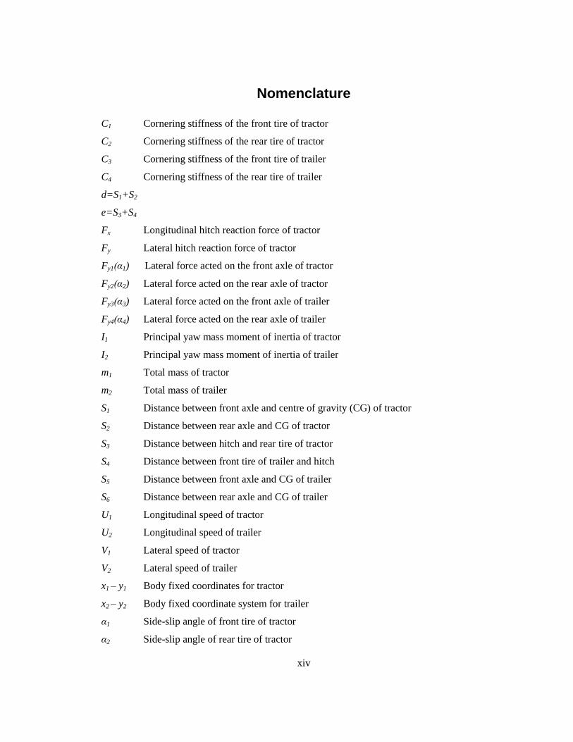
Nomenclature

C1 Cornering stiffness of the front tire of tractor

C2 Cornering stiffness of the rear tire of tractor

C3 Cornering stiffness of the front tire of trailer

C4 Cornering stiffness of the rear tire of trailer

d=S1+S2

e=S3+S4

Fx Longitudinal hitch reaction force of tractor

Fy Lateral hitch reaction force of tractor

Fy1(α1) Lateral force acted on the front axle of tractor

Fy2(α2) Lateral force acted on the rear axle of tractor

Fy3(α3) Lateral force acted on the front axle of trailer

Fy4(α4) Lateral force acted on the rear axle of trailer

I1 Principal yaw mass moment of inertia of tractor

I2 Principal yaw mass moment of inertia of trailer

m1 Total mass of tractor

m2 Total mass of trailer

S1 Distance between front axle and centre of gravity (CG) of tractor

S2 Distance between rear axle and CG of tractor

S3 Distance between hitch and rear tire of tractor

S4 Distance between front tire of trailer and hitch

S5 Distance between front axle and CG of trailer

S6 Distance between rear axle and CG of trailer

U1 Longitudinal speed of tractor

U2 Longitudinal speed of trailer

V1 Lateral speed of tractor

V2 Lateral speed of trailer

x1 – y1 Body fixed coordinates for tractor

x2 – y2 Body fixed coordinate system for trailer

α1 Side-slip angle of front tire of tractor

α2 Side-slip angle of rear tire of tractor

xv

α3 Side-slip angle of front tire of trailer

α4 Side-slip angle of rear tire of trailer

δ Steering angle of front tire of tractor

δr Steering angle of front tire of trailer

ω1 Yaw rate of tractor

ω2 Yaw rate of trailer

ψ Articulation angle between tractor and trailer

1

Chapter 1

INTRODUCTION

1.1 WHY ARE ARTICULATED HEAVY VEHICLES WIDELY USED?

The majority of articulated heavy vehicles (AHVs) are commonly used for the

transportation of goods and materials because of their cost effectiveness in both labor

requirements (mainly the driver) and fuel consumption. An AHV is a substitute to a

number of single units, since it is an assemblage of two or more rigid (i.e. non-

articulating) vehicle units [1]. An AHV, therefore, moves more payloads with lower tare

weight than a single unit vehicle, with only one driver. Moreover, compared with single

unit vehicles, AHVs greatly reduce greenhouse gas emissions. Thus, the trucking industry

all around the world has demonstrated incredible commercial attractiveness of AHVs.

1.2 VEHICLE CONFIGURATIONS

In an AHV, adjacent units are connected through mechanical couplings, such as pintle

hitches, dollies, and 5th

wheels. The towing unit is called tractor and it usually has one or

more steerable axles controlled by the driver. Each of the following vehicle units is called

a trailer. There are two major groups of trailers: semi-trailers andfull trailers. A semi-

trailer is supported vertically by its tractor at the front and the rear end is connected to the

rear running gear. In afull trailer, on the other hand, the front support from the towing

unit is replaced by its front running gear.

2

1.3 MOTIVATION

The popularity and application of AHVs is growing rapidly because of their great

commercial benefits. However, the handling characteristics of AHVs are more complex

than those of single unit vehicles, as neighboring units affect each other due to inner

forces acting at their articulated point [2]. In addition to this, due to their large sizes and

heavy weights, the operation of AHVs has been of primary concern to highway safety

[3]. Consequently, the design of an AHV is a challenging task. The key reason of AHVs‟

intricate dynamics is the articulated joints through which the neighboring vehicle units

interact with each other. The distinguished dynamics features of AHVs may lead to

unstable motion modes [4]. These unstable motion modes may cause hazardous

accidents. In the US, more than 35,000 people were killed in road accidents each year

from 1993 to 1998 [5]. Among them, about 10% were the results of the unstable motion

modes of AHVs. These unstable motion modes become dominant at high speeds.

The unstable motion modes of AHVs can be classified into three types. The first type

is called jack-knifing, mainly caused by the uncontrolled large relative angular motion

between adjacent units. It often results in the lateral slip of rear axles of the leading unit.

The jack-knifing motion mode is a main reason for dangerous traffic accidents. When the

articulation angle reaches a certain limit, it becomes incredibly difficult for the driver to

control the vehicle by steering the tractor.

The second type of unstable motion modes is the lateral oscillation of trailers, called

trailer sway. This unstable motion mode is usually experienced when design variables

3

and/or operating parameters are chosen very close to their critical values. In this case, a

very little amount of disturbances acting on the vehicle, e.g., side wind gust, abrupt

steering effort by the driver, etc., may cause the lateral oscillation [6]. This may result in

the loss of stability and the vehicle becomes self-excited due to non-conservative forces

[7]. For AHVs, these non-conservative forces may arise at the contact point between tire

and road due to lateral forces, aligning torques and longitudinal forces [8].

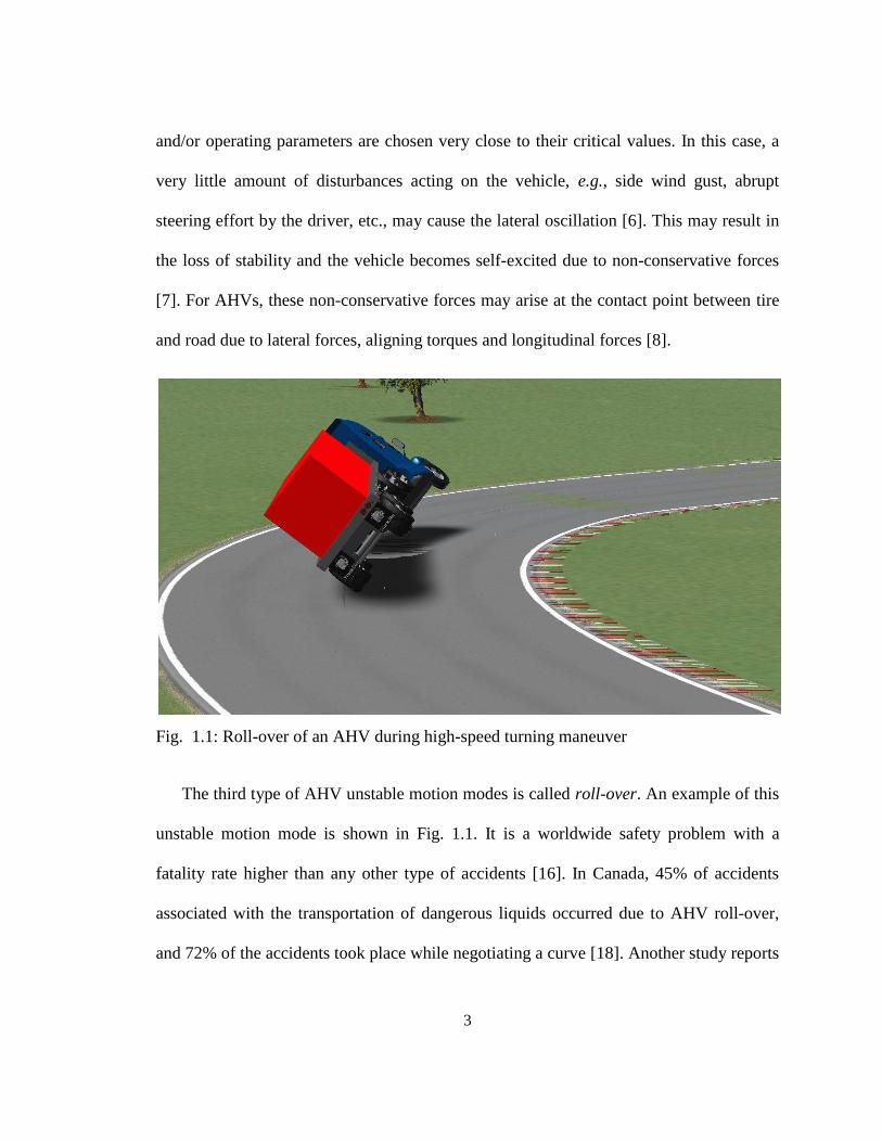
Fig. 1.1: Roll-over of an AHV during high-speed turning maneuver

The third type of AHV unstable motion modes is called roll-over. An example of this

unstable motion mode is shown in Fig. 1.1. It is a worldwide safety problem with a

fatality rate higher than any other type of accidents [16]. In Canada, 45% of accidents

associated with the transportation of dangerous liquids occurred due to AHV roll-over,

and 72% of the accidents took place while negotiating a curve [18]. Another study reports

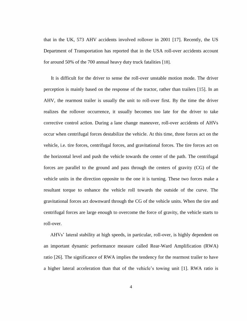
4

that in the UK, 573 AHV accidents involved rollover in 2001 [17]. Recently, the US

Department of Transportation has reported that in the USA roll-over accidents account

for around 50% of the 700 annual heavy duty truck fatalities [18].

It is difficult for the driver to sense the roll-over unstable motion mode. The driver

perception is mainly based on the response of the tractor, rather than trailers [15]. In an

AHV, the rearmost trailer is usually the unit to roll-over first. By the time the driver

realizes the rollover occurrence, it usually becomes too late for the driver to take

corrective control action. During a lane change maneuver, roll-over accidents of AHVs

occur when centrifugal forces destabilize the vehicle. At this time, three forces act on the

vehicle, i.e. tire forces, centrifugal forces, and gravitational forces. The tire forces act on

the horizontal level and push the vehicle towards the center of the path. The centrifugal

forces are parallel to the ground and pass through the centers of gravity (CG) of the

vehicle units in the direction opposite to the one it is turning. These two forces make a

resultant torque to enhance the vehicle roll towards the outside of the curve. The

gravitational forces act downward through the CG of the vehicle units. When the tire and

centrifugal forces are large enough to overcome the force of gravity, the vehicle starts to

roll-over.

AHVs‟ lateral stability at high speeds, in particular, roll-over, is highly dependent on

an important dynamic performance measure called Rear-Ward Amplification (RWA)

ratio [26]. The significance of RWA implies the tendency for the rearmost trailer to have

a higher lateral acceleration than that of the vehicle‟s towing unit [1]. RWA ratio is

5

defined as the ratio of the peak lateral acceleration at the rearmost trailer‟s CG to that of

the vehicle‟s towing unit in an obstacle avoidance lane-change maneuver [4, 27]. In a

general sense, the lower the RWA ratio, the higher the vehicle lateral stability [55].

The above unstable motion modes refer to high speed directional performance issues.

Interestingly, the high speed issues of AHVs are conflicting with those at low speeds in

meeting the relevant AHV standards. Australian performance-based standards (PBS)

[36], for example, describes the performance issues related to both high- and low-speed

AHV operations. At low speeds the main directional performance measure is the path-

following ability of rearmost unit. In general, AHVs‟ rear unit faces difficulties in

tracking the lead unit‟s path. In an AHV, where the rearmost axle cannot steer during a

turn, the rear tires follow different paths as from those of the steering tires of the towing

unit. The commonly used performance measure for low-speed path-following is called

Path-Following Off-Tracking (PFOT) [1]. This PFOT has been observed since the first

time multi-axle vehicles were built [22].

AHVs‟ complex configurations and large sizes lead to poor path-following

performance while traveling at low speeds on a local road and city streets [10]. The

amount of PFOT of each unit is proportional to the square of its wheelbase [1]. This poor

path-following ability is the source of tire scrub against the road during tight cornering

maneuvers. The tire scrub damages both the tire and road surfaces [28]. Moreover,

inferior path-following capability of AHVs rises safety concerns for the neighboring

traffic and damage of road infrastructure [29]. PFOT is defined as the maximum radial

6

offset between the path of the tractor‟s front axle centre and that of the trailer‟s rear axle

centre during a specific maneuver [30]. Note that besides wheelbase the PFOT is also

dependent on other factors, such as forward speed [21].

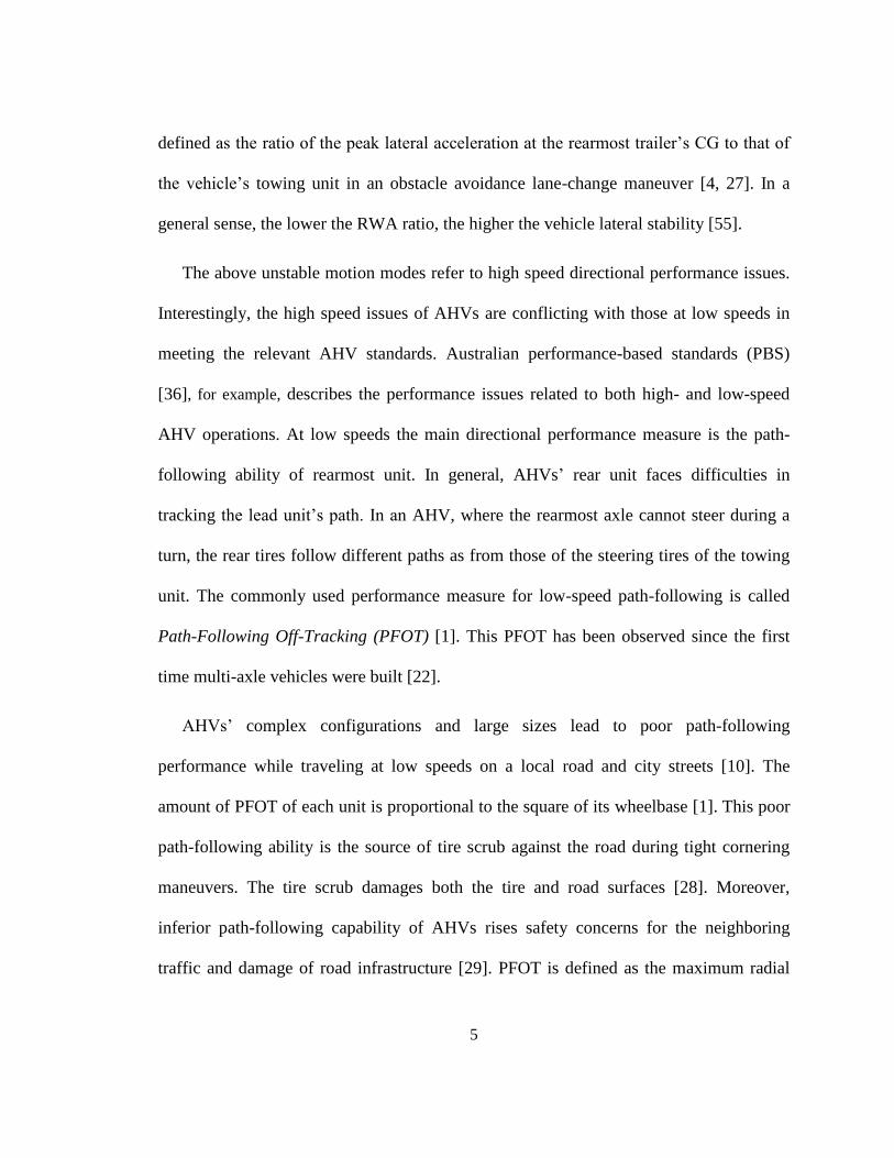
Fig. 1.2: High speed Path-Following Off-Tracking during constant radius turn maneuver

Australian PBS also specifies high speed path-following limits termed as high speed

Path-Following Off-Tracking (PFOT). Both types of PFOT are briefly discussed below

as a comparison basis:

High speed PFOT, as shown in Fig. 1.2, is the result of centrifugal force. It is

observed that a vehicle travels at higher forward speeds, and the rear axle pulls

outward from the steering axle path during a turn or lane change maneuver.

Excessive high speed PFOT may cause a dangerous accident.

7

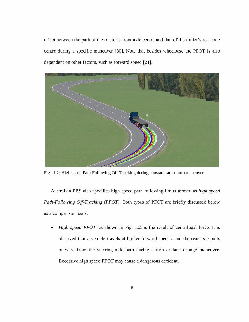
Low-speed PFOT, as shown in Fig. 1.3, is mainly determined by the geometric

features of AHVs. In low or moderate speed turns, the rear tires are pulled inward

of the curved path. The longer the wheelbase of a unit or the tighter the turn, the

higher the PFOT. Some researches on traffic accident prove that PFOT is a crucial

problem for safe vehicle operations [22]. The design of pavements, roads, parking

lots and trucking yards requires more land areas to ensure the safety operations of

AHVs.

Fig. 1.3: Low speed Path-Following Off-Tracking

Among all these performance measures associated with high-speed AHV safe

operations, the RWA ratio is critical. However, at low speeds, the PFOT error becomes

the dominating concern. RWA ratio at high speeds and PFOT at low speeds are the main

performance measures for stability and maneuverability, respectively. These two

8

performance measures are conflicting. Thus contradictory design goals may be the most

fundamental and important in the design of AHVs. The coordinating of these conflicting

design goals will be the main task of this thesis.

1.4 THESIS CONTRIBUTIONS

To solve the contradictory design problem, proposed a variety of passive or active trailer

steering (ATS) systems. These studies focused on identifying the effects of either passive

or active trailer steering systems using dynamic simulation and analysis. These studies do

not address adequately the trade-off relationship between path-following ability at low

speeds and stability at high speeds in their design synthesis approaches. In conventional

dynamic analysis of active trailer steering (ATS) systems of AHVs, the passive vehicle

system is designed first from mechanical viewpoint. Then, the ATS systems are designed

and added onto the vehicle already designed. This sequential design approach may not

achieve optimal trade-off solutions between the contradictory performance requirements

of AHVs [12].

In this thesis, a new design synthesis approach is proposed: with design optimization

techniques, the active design variables of ATS systems and passive design variables of

trailers can be optimized simultaneously; the ATS controller derived has two operational

modes, one for improving lateral stability at high speeds and the other for enhancing

path-following at low speeds. To demonstrate the effectiveness of the proposed approach,

it is applied to the design of an ATS system for a tractor/full-trailer combination based on

9

a 3 degree of freedom (DOF) linear yaw plane model. It is expected that the proposed

approach can be used for identifying desired design variables and predicting performance

envelopes in the early design stages of AHVs with ATS systems. Moreover, an optimal

controller for the ATS system is proposed based on the preview information of lateral

position deviation of preceding axle centers.

1.5 THESIS ORGANIZATION

In this thesis two different optimization design methods for AHVs are examined

and investigated. Chapter 1 serves as an introductory chapter, providing general

background information of different performance measures of AHVs. Chapter 2

offers the state-of-the-arts of researches on the design of AHVs with ATS systems.

Chapter 3 introduces the relevant vehicle models, basic control technique, and one

optimization algorithm. Chapter 4 presents a two design loop (TDL) method for

predicting design envelop of AHVs by selecting both active and passive design

variables. Chapter 5 describes another design method, called single design loop

(SDL), where both active and passive variables are optimized simultaneously. In

this chapter the SDL method is also compared with the TDL method. Chapter 6

presents the design of an optimal ATS controller based on the preview information

of lateral position deviations of preceding axle center. Chapter 7 concludes the

thesis, summarizing its findings and providing suggestions for future work in the

field of the current research.

10

Chapter 2

LITERATURE REVIEW

2.1 INTRODUCTION

This chapter offers a comprehensive literature review of the state-of-the-art of AHVs

design. More attention is directed towards the design of ATS system.

The last two decades have witnessed the advances in trying to find solutions to the

contradictory design goals of maneuverability at low speeds and lateral stability at high

speeds. A variety of passive trailer steering systems have been developed. However,

these systems can only improve low-speed maneuverability of AHVs. Recently, a lot of

efforts have been focused on the development of active trailer steering systems.

Numerical simulations show that active trailer steering system can achieve acceptable

levels of RWA and PFOT [29].

2.2 PASSIVE TRAILER STEERING SYSTEMS

Aurell and Edlund examined the influence of the location of passive steered axles on the

dynamic stability of a tractor/semi-trailer system [31]. Jujnovich and Cebon compared the

performance of various passive trailer steering systems [32]. Results derived from these

studies imply that identifying optimal design variables, such as the trailer length, axle

11

group location and weight distribution etc., can lead to the improvement of both high and

low speed performance.

2.2.1 Low-Speed Maneuverability

In order to improve low-speed path-following of AHVs, several passive trailer steering

systems, including self-steering, command steering, and pivotal bogie mechanisms, have

been developed [25]. It is found that these passive trailer steering systems can improve

path-following ability at low speeds. A comparative study of self-steering, command

steering, and pivotal bogie systems was conducted by Sanker et al. [43]. In their study,

the command steering, also called force steering, system is used. These passive systems

implement trailer steering based on a geometric relationship with articulation angle or a

tire force balance. In this passive steering system, the steering angle of a rear axle is

considered as proportional to the articulation angle. The directional dynamics analysis of

self-steering and command steering systems of a tractor semi-trailer combination reveals

that the Path-Following Off-Tracking (PFOT) is significantly reduced at low speeds.

These trailer steering systems also substantially reduce lateral tire forces. As a result, an

AHV with passive steering system is more maneuverable, and able to access more of the

road network. They reduce tire wear and also decrease the damage of the road surface

whilst turning compared to conventional fixed-axle semi-trailer. However, their study

also reported that, at low-speed, passive steering system may increase the amount of tail

swing.

12

2.2.2 Poor High-Speed Stability

Although at low-speeds the AHVs, with passive steering systems, exhibit improved

performance, at high-speed their stability decreases [1, 28]. Jujnovich and Cebon [32]

also reported that the high-speed performance measures, in both Rear-Ward

Amplification (RWA) ratio and transient PFOT, are low with passive steering systems.

This results support the rules of thumb suggested by Fanchar and Winkler [1] that “what

one does to improve low-speed performance is likely to degrade high-speed performance

and vice versa”. As previously mentioned, articulated heavy vehicles (AHVs) exhibit

unstable motion modes at high speeds, including jack-knifing, trailer swing and roll-over

[25]. These unstable motion modes may lead to fatal accidents. Thus, at high-speed these

passive steering systems might cause serious traffic accidents.

To tackle this problem, it is a common practice that passive trailer steering systems

are locked in high-speed operations.

2.3 ACTIVE TRAILER STEERING SYSTEMS

The last two decades have witnessed the advances in trying to find solutions to the

contradictory design goals of path-following at low speeds and lateral stability at high

speeds. A number of active trailer steering (ATS) systems have also been proposed for

reducing Path-Following Off-Tracking (PFOT) at low speeds [29, 30, 49, 50]. In 2003,

Wu and Lin [33] studied the dynamic effect of a multi-axle full- trailer with an active

steering system using yaw-plane model. The front steering axle of trailer is able to reduce

PFOT using a fixed steer ratio. The steer ratio is a multiplying factor to tractor steering

13

angle to determine the trailer axle steering angle. This study also provides an interesting

phenomenon that, with the introduction of a multi-axle steering system, the transient

PFOT is reduced in a high-speed lane change maneuver. A similar phenomenon is also

reported in the results of Rangavajhula‟s simulations on ATS systems [49]. The yaw

plane model of a tractor/full-trailer system was extended to include threefull trailers with

steerable trailer axles in their research. They also used a similar steer ratio for steering the

trailers and showed that with a given steering input from the tractor driver, the radius of a

90-degree intersection turn was drastically reduced in comparison to non-steerable trailer

system. Rangavajhula and Tsao [29] also studied the cost effectiveness of various

combinations with different active trailer steering axles. Their study concludes that the

ATS system with only the first and second trailer steerable axles is the most cost effective

for an AHV with threefull trailers.

2.3.1 RWA Ratio as a Control Criterion

El-Gindy et al. used RWA ratio as a control criterion in the design of active yaw

controllers for a tractor/full-trailer combination [4]. It is demonstrated that compared with

the baseline vehicle, the one with the active trailer yaw controller can reduce the RWA

level without significant change of the baseline vehicle trajectory. Rangavajhula and Tsao

also used RWA ratio as the control criterion in the design of optimal trailer steering

controllers based on the linear quadratic regulator (LQR) technique [29, 30]. Numerical

simulations show that active trailer steering systems can achieve acceptable levels of

RWA and PFOT. Interestingly, they proved that ATS system improves high-speed

14

performance also. Their research illustrates that the ATS system not only improves low-

speed maneuverability, but also enhanced high-speed stability during a lane change

maneuver by reducing Rear-Ward Amplification (RWA) ratio.

2.3.2 Simulation Environments

However, Wu et al. [33], and Rangavajhula et al. [29, 30, 49, 50] performed the

simulation of high-speed single lane change maneuver by considering the forward speed

as 55 km/h. The open-loop steering input is a single sinusoidal wave with a 4 second time

period. However, the ISO [51] and SAE standards [52] suggest that the forward speed

during high speed lane change test should be 88 km/h and the open-loop steering input

should be a single sinusoidal wave with a 2.5 second time period. To effectively evaluate

the high-speed lateral stability of AHVs, the selected vehicle forward speed of 55 km/h is

not reasonable.

Moreover, their research is based on the design criterion: the lower the RWA ratio,

the better the high-speed stability of AHVs. However it is argued that RWA ratio of 1.0 is

ideal for the trailing units to follow the motion of the tractor in a multi-trailer articulated

vehicle. A low RWA ratio, e.g. 0.1, may degrade the path-following ability of the

vehicle.

To assume safe operating conditions in obstacle avoidance situations on highways,

the following performance requirements should be considered: 1) to avoid the obstacle,

all vehicle units of the AHV should respond the driver steering input quickly and

adequately; and 2) no unit should be allowed to roll-over. If the RWA ratio is much

15

greater than 1.0, the rear unit will roll-over at a relatively low level of lateral acceleration.

However, if the RWA is much less than 1.0, the rear unit will not follow the path of the

lead unit around the obstacle.

2.3.3 Passive and Active Steering System Together

To improve compatibility between low-speed PFOT and high-speed RWA, researchers

have investigated a variety of potential solutions. It is reported that the location of steered

axles and the types of steering mechanism have significant effects on the dynamic

stability of a tractor/trailer system [31]. The RWA ratio has been used as a control

criterion in the design of active yaw controllers for a tractor/full-trailer combination [4].

Recently, the linear quadratic regulator (LQR) technique has been applied to the

controller design of ATS systems for AHVs [29, 30]. The researchers intended to identify

the correlation between the RWA ratio and the PFOT value in order to reduce the latter

through minimizing the former. Another solution accepted to date is to use a passive and

an active trailer steering system [4, 28, 30]. At low speeds, the passive steering systems

are employed in order to effectively decrease PFOT values. From medium to high speeds,

ATS systems are applied to ensure that AHVs have high stability. This solution provides

a good way to coordinate the conflicting design criteria at low and high speeds, but it

increases the complexity of trailer configurations since the „dual‟ steering systems co-

exit.

16

2.4 CONTROLLER DESIGN FOR ATS SYSTEMS

El-Gindy et al. used RWA ratio, as a control criterion, in the design of active yaw

controllers for a tractor/full-trailer combination [4]. The vehicle under consideration was

a six-axle tractor/full trailer combination, which usually exhibits a high level of RWA

leading to roll-over during obstacle avoidance maneuvers.

In their research, several control strategies were investigated to improve high-speed

stability: active yaw control at the truck CG, active yaw control at the dolly CG, and

active yaw control at the trailer CG. They investigated all those control techniques both

individually and in combination. The outcome of the active control torque applied to

different vehicle units of AHV was examined via an optimal linear quadratic regulator

(LQR) approach incorporated with a simplified 4 degrees-of-freedom linear vehicle

model. The controller performance index parameters were estimated using an ad-hoc

fashion based on acceptable RWA target values. The sensitivity of the controller to tyre

cornering stiffness variation, of percent of their nominal values, was further

investigated. Their simulation results indicated that the RWA could be decreased, when

active yaw torque was applied to the dolly, without significant change of the trajectory of

uncontrolled vehicle. The controller could be more efficient, if applied to the lead unit or

to the rearward unit, in enhancing the dynamic performance and roll stability. The

trajectory of the AHV became greatly affected and driving difficulties was also

experienced. For active yaw control at the dolly CG, the optimal controller was found to

be most sensitive to the cornering stiffness variation of dolly tyre and least sensitive to

steering axle from the Rear-Ward Amplification level. They also found that the controller

17

was greatly sensitive to steering axle parameter variations for path following ability of

the vehicle.

Differential breaking is used by Fancher et al. [59] to control the lateral stability at

high speeds reducing snaking unstable motion modes. Their control strategy of

commanding brake pressures to the axle tires was such that yawing of the dolly could

steer thefull trailer along with controlling the lateral acceleration. With sinusoidal driver

steering input of a 2.5 second period they improved the vehicle high-speed performance

by reducing RWA ratio from value of 2.3 to 1.7. In their studies, the desired RWA ratio

was 1.0. The Rear-Ward Amplification suppression system should not be on all of the

time, as it might cause excessive use of compressed air or cause the brakes to overheat

and wear excessively, even if the amount of braking were not slight.

Tanaka [57] used a fuzzy controller to control the backward movement of a

tractor/semi-trailer system via a model-based fuzzy control technique. Takagi–Sugeno

fuzzy modeling [48] approach was applied to nonlinear dynamic model of AHV. They

studied AHVs for low speed jackknife preventive backward path-following issues. A

nonlinear dynamic vehicle model was developed based on a Takagi–Sugeno fuzzy model.

The idea of parallel distributed compensation was utilized to estimate a fuzzy controller

from the Takagi–Sugeno fuzzy model of the vehicle. To ensure the controller stability of

their proposed system, they used Lyapunov method. The stability conditions were

characterized in terms of linear matrix inequalities since the stability analysis is decreased

to a problem of finding a common Lyapunov function for a set of Lyapunov inequalities.

18

Both their simulation and experimental investigations showed that the designed fuzzy

controller effectively achieved the backward movement control of the articulated vehicle.

Recently, linear quadratic regulator (LQR) technique was applied to the controller design

for ATS systems of multi-trailer articulated heavy vehicles in order to improve both low-

speed maneuverability and high-speed stability [30, 29]. Numerical simulations show that

ATS systems can achieve acceptable levels of RWA ratio and PFOT. However, in the

LQR controller construction, the design criteria were not clearly explained and justified.

It was indicated that the trailer tires could be steered through an angle proportional to the

single-point path preview lateral position error and results illustrated that the preview

controller provided a moderate tracking capability [67]. A path-following steering

controller in the discrete time domain was developed for an ATS system of a semi-trailer

for improving both maneuverability at low-speeds and stability at high-speeds [69]. The

controller steered the semi-trailer tires and the trailer rear end followed the trajectory of

the 5th

wheel at all speeds. However, the applicability of the controller to afull trailer has

not been addressed.

2.5 LIMITATIOINS OF EXISTING DESIGN AND ANALYSIS

METHODS

All the above studies focused on identifying the effects of either passive or active trailer

steering systems on the contradictory design goals based on dynamic simulation and

analysis. However, these studies have not addressed the trade-off relationship between

19

path-following at low speeds and later stability at high speeds using design synthesis

approaches. In these dynamic analyses of active trailer steering (ATS) systems of AHVs,

it was assumed that the passive vehicle system was designed first and then the ATS

systems developed were added onto the vehicle originally designed from a purely

mechanical viewpoint. This sequential design approach may not achieve optimal trade-

off solutions between the contradictory performance requirements of AHVs [23].

Past studies mainly focused on investigating the effects of key design variables and

influence of either passive or active trailer steering systems on the contradictory design

goals based on dynamic simulation and analysis. This is a trial and error approach, where

designers iteratively change the values of design variables and reanalyze until acceptable

performance criteria are achieved. For example, in the LQR controller design for ATS

systems, this approach is commonly used to determine desired weighting factors for the

cost function. This manual design process is tedious and time-consuming. With the

stringent conflicting performance requirements, the design of AHVs should switch from

pure simulation analysis to extensive design synthesis.

To address the limitations of the existing design and analysis approaches, the thesis

will investigate innovative methods for the design of AHVs with ATS systems.

20

Chapter 3

VEHICLE MODELING AND DESIGN TOOLS

3.1 INTRODUCTION

This thesis will focus on addressing design synthesis methods for AHVs with ATS

systems. To examine and evaluate these methods, they will be applied to the design of a

tractor/full-trailer system with ATS system. In this chapter, the relevant vehicle models,

the basic control technique, and one optimization algorithm are briefly introduced.

3.2 VEHICLE MODELING

To predict vehicle dynamic behaviors, two vehicle models, namely Model-1 and Model-2

are introduced in the design synthesis of AHVs with ATS systems.

3.2.1 Model-1

In order to evaluate the high-speed lateral stability and low-speed path-following of the

tractor/full-trailer combination, the 3-DOF linear yaw plane model [33, 34] is outlined in

this section.

21

r

6S

2V

2

xF

yF

1

1U

1V

2S3S

)( 11yF

)( 22yF

)( 3

3yF

)(

4

4yF

2U

2x

2y

1x

1y

5S

4S

1S

xF

yF


Model-1

The articulated vehicle consists of a tractor/full-trailer, which are connected by a

hinge pin. As shown in Fig. 3.1, the system is telescoped laterally and each axle set is

represented by one tire. Based on the body fixed coordinate systems and

for the tractor and trailer, respectively, the governing equations of the system can be

derived. The motions considered are tractor lateral velocity , tractor yaw rate and

articulation angle between the tractor and trailer. In this model, aerodynamic forces,

rolling and pitching motions, and longitudinal forces between tire and road are ignored.

From Newton‟s laws of dynamics, the equations of motion for the tractor are written as

22

(3.1a)

(3.1b)

(3.1c)

and the equations of motion for the trailer are cast as

(3.2a)

(3.2b)

(3.2c)

where the notation is given in Appendix A.

To derive the simplified vehicle model, the following assumptions have been made: 1)

the forward speed remains constant; 2) the tractor steering angle is small; 3) the

articulation angle is small; 4) all products of variables are ignored; 5) the lateral tire

force )( iyiF is linear functions of sideslip angle , . The velocities of the

pin using either of the coordinate systems should be compatible. Eliminating the coupling

reaction forces and from equations (3.1) and (3.2) leads to the following 3-DOF

linear yaw plane model expressed in the state space form as

(3.3)

where the matrices , , and are provided in Appendix B. The state vector and

control vector are expressed as

23

(3.4)

and

(3.5)

Note that is the control vector related to the trailer front axle tire steering angle.

3.2.2 Model-2

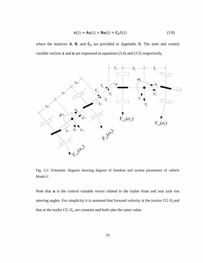
As shown in Figs. 3.1 and 3.2, the only difference between Model-1 and Model-2 is the

rear axle of the trailer. In the case of Model-1, the tire on this axle is non-steerable, while

in the case of Model-2, the tire on this axle is steerable. For Model-2, the equations of

motion for the trailer are listed as follows,

(3.6a)

(3.6b)

(3.6c)

and the equations of motion for the trailer are cast as

(3.7a)

(3.7b)

(3.7c)

The state space form to equations (3.6) and (3.7) are expressed as

24

(3.8)

where the matrices , , and are provided in Appendix B. The state and control

variable vectors and are expressed in equations (3.4) and (3.5) respectively.

6S

2V

2

xF

yF

1

1U

1V

1S

)( 11yF)( 22yF

)( 3

3yF

)(

4

4yF

2U

2x

2y

1x

1y

f

r

xF

yF5S

4S

2S3S


Model-2

Note that is the control variable vector related to the trailer front and rear axle tire

steering angles. For simplicity it is assumed that forward velocity at the tractor CG and

that at the trailer CG are constant and both take the same value.

25

3.3 TEST MENEUVERS

To evaluate AHVs‟ performance levels in high-speed RWA ratio and low-speed Path-

Path-Following Off-Tracking (PFOT), two types of simulations have been used: open-

loop and close loop simulation.

3.3.1 Open-Loop Simulation

The first type is based on an open-loop control approach with specified steer inputs,

including pulse and step steer inputs. These simulations require the precise application of

a predetermined steer sequence and the resultant vehicle responses are observed. To

assess the RWA and path-following levels, respectively, one-period sinusoidal steer

inputs [29-31, 33] and step steer inputs [29, 30] have been used accordingly.

High-Speed Case

A single lane change maneuver is simulated for determining the high-speed RWA

ratio. In the simulation, the vehicle is traveling at the speed of 88 km/h along a straight

path and a sudden lane change is conducted. The lateral displacement of the vehicle in the

lane change is 3.7 m. The steering input, in radians, for this maneuver takes a single

sinusoidal wave as

(3.9)

where the period is 2.5 seconds and the value of amplitude is selected in such a way

that the vehicle is able to complete the single lane change.

Low-Speed Case

26

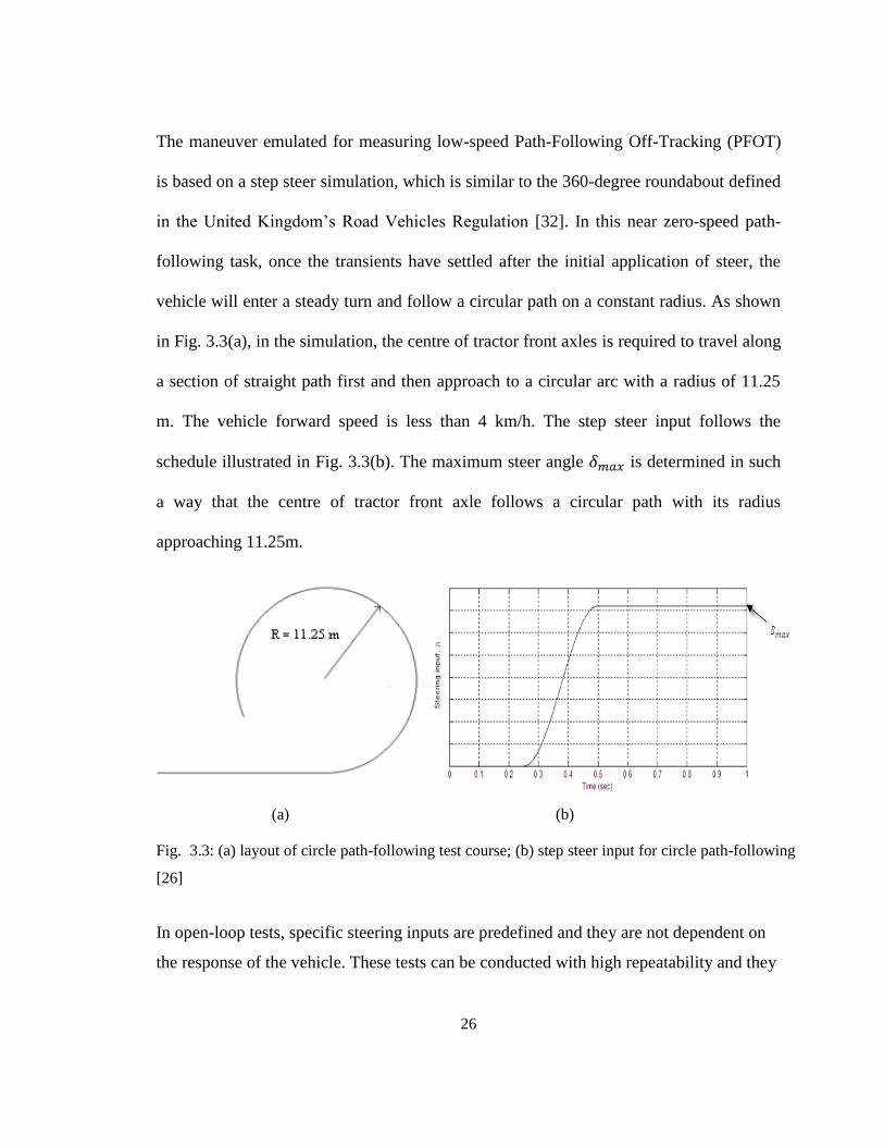
The maneuver emulated for measuring low-speed Path-Following Off-Tracking (PFOT)

is based on a step steer simulation, which is similar to the 360-degree roundabout defined

in the United Kingdom‟s Road Vehicles Regulation [32]. In this near zero-speed path-

following task, once the transients have settled after the initial application of steer, the

vehicle will enter a steady turn and follow a circular path on a constant radius. As shown

in Fig. 3.3(a), in the simulation, the centre of tractor front axles is required to travel along

a section of straight path first and then approach to a circular arc with a radius of 11.25

m. The vehicle forward speed is less than 4 km/h. The step steer input follows the

schedule illustrated in Fig. 3.3(b). The maximum steer angle is determined in such

a way that the centre of tractor front axle follows a circular path with its radius

approaching 11.25m.

(a) (b)

Fig. 3.3: (a) layout of circle path-following test course; (b) step steer input for circle path-following

[26]

In open-loop tests, specific steering inputs are predefined and they are not dependent on

the response of the vehicle. These tests can be conducted with high repeatability and they

27

are used for the purpose of characterizing only vehicle responses. Open-loop tests ignore

human/vehicle interactions and thus only provide limited useful information.

3.3.2 Closed-Loop Simulation

The second type is essentially a closed-loop steer control process. In these simulations, a

driver model is introduced and the vehicle model follows a well-defined path under the

control of the driver model. During the process, the combined driver/vehicle models‟

responses are observed. To determine the RWA ratio of AHVs with semi-trailer steering

systems based on the lane change maneuver recommended by SAE [35], a driver model

has been used [32].

In closed-loop tests, a desired vehicle motion or trajectory is achieved by

continuously monitoring vehicle response and adjusting steering actions accordingly. In a

closed-loop test, the driver is considered as an integral part of the system to the extent

that the mathematical model of the entire system involves a driver model [32]. Because

of the cost and safety concerns, it may not be practical to perform field testing.

Simulation assessment thus may be more practical in certain situations. Moreover,

computer simulations provide an efficient means to analyze the interaction between the

human driver and the vehicle, even before a vehicle or its subsystems are produced. In

past studies on ATS systems for AHVs, only the open-loop tests were simulated to

evaluate the vehicle‟s performance measures in RWA ratio and PFOT value [12, 29, 30,

33]. Obviously, these studies cannot provide sufficient information regarding the

interaction between the human driver and the ATS systems in computer-based vehicle

design processes. Thus, in the current research, to demonstrate the efficacy of the

28

proposed design synthesis approach, a simplified driver model has been generated and

the closed-loop tests have been simulated for evaluating vehicles‟ directional

performance.

3.4 LINEAR QUADRATIC REGULATOR TECHNIQUE

In this thesis, the controllers designed for ATS systems are mainly based on the linear

quadratic regulator (LQR) technique.

The LQR is introduced by Kalman in Ref. [63] and [64]. The infinite horizon LQR

problem considers the linear time-invariant plant

(3.10)

where is the state matrix, is the input matrix, is the state

vector, and is the control vector. The time-invariant quadratic cost functional

(3.11)

with

and (3.12)

and the desired feedback controls of the form

(3.13)

The sufficient condition for the optimality is given by

29

(3.14)

and for arbitrary admissible

(3.15)

It is easy to see that (3.13) and (3.14) are satisfied by

(3.16)

and

(3.17)

provided

(3.18)

The above equation (3.18) is known as the Algebraic Ricatti Equation (ARE).

3.5 GENETIC ALGORITHMS

As will be discussed in Chapter 4 and 5, a genetic algorithm (GA) will be the basic

optimal search algorithm used in the design synthesis methods. Thus, the characteristics

of GAs are briefly introduced.

Evolutionary computation or evolutionary computing represents a broad area that

covers a family of adaptive search population based methods that can be applied to the

optimization of both discrete and continuous mappings. They have different features from

the typical single-point-based optimization techniques, such as gradient search techniques

30

and other directed search techniques [60], by the fact that their search mode is executed

based upon multiple positions in the search space rather than upon a single position.

Genetic algorithm is one of the very attractive methods of this computational paradigm

[61].

3.5.1 Genetic Algorithm and Optimization

The GA search optimization algorithm was formulated first by Holland [62]. This is a

derivative-free based technique which makes it applicable to smooth functions, simply

continuous functions, or even discontinuous functions. This efficient search technique,

especially to achieve global optima, is based on biologic evolution and on the survival of

the fittest principal. This algorithm evaluates the function at a set of points in the

function‟s variable space, usually chosen randomly within their allocated search range.

This aspect makes them good candidates for solving global optimization problems and

makes them less vulnerable to local optima. The solution is reached based on iterative

search procedure, and as such mimics to a certain extent the evolution process of

biological entities. To understand this genetic algorithm properly, two most important

terms are defined: the genotype of a population and its fitness value.

3.5.2 Genotype

In artificial evolution the “data” of the system considered is approximated as a living

creatures in the framework of natural evolution. In nature, each individual represents a

potential solution to the challenge of survival, while in GA a set of potential solutions are

considered. This collection is termed as a population and each single solution is called an

31

individual. Each individual in nature has a form which is determined by its DNA and its

set of genetic train is referred to as a genotype. The term genotype, in GA, represents the

encoding of a problem solution denoted by an individual. Many individuals in a

population may have the same or similar genotypes. An individual‟s genotype is termed,

in GA, as its chromosome. Strings, also called bits or characters, are normally used to

represent genotype in GA. Each single unit of genetic information is referred as gene

which is determined by each element of the string.

In nature, these genes control various traits in the individual. In humans, genes

determine, for example, eye and hair colour and also numerous other characteristics. In a

genetic algorithm, a solution encoding also may make use of several interacting genes.

Each gene consists of one or more possible values, called alleles. If a specific gene

represents eye color, each allele represents each color for that gene: brown, black, blue

etc. For a particular gene, the number of alleles is fixed in nature, while it is determined

by the encoding of solutions in artificial evaluation. The number of gene in a genotype is

fixed in genetic algorithm.

3.5.3 Fitness Function

The fitness of a creature in nature refers to its ability to survive in its environment. In GA,

it represents the value or goodness of a particular solution. A “fitter” creature is able to

find food and shelter better than another. Similarly, the fitness of an individual solution

leads the concept of fitness function, also called objective function. An objective function

denotes a genotype as its parameter and gives usually a real valued outcome that refers to

32

the fitness or goodness of the solution. The choice of this objective function is very

crucial.

3.5.4 Genetic Algorithm Operators

The technique, a composition of a population changes, is the most important feature of an

evolutionary algorithm. Three major forces, in nature, are: natural selection, mating, and

mutation. In GA, the corresponding forces are: selection, crossover, and mutation. They

are known as genetic operators, and act on individuals, sets of individuals, populations,

and genes.

3.5.4.1 Selection

With this procedure an individual is selected that take part in reproduction procedure to

give birth to the next generation. Selection operators typically serve to eliminate

weaklings from a population, or to select strong individuals for reproduction. These

stochastic selection operators probabilistically select good solutions, and eliminate bad

ones based on the evaluation given to them by the objective function. The elitist model is

considered as a part of several heuristics where a number of populations are chosen for

further processing. The ranking model of this process ranks each member of population

depending on its fitness value. The roulette tire procedure assigns a probability to each

individual for reproduction. Then the cumulative probability is determined

for each . If becomes greater than a random number , corresponding individual is

selected.

33

3.5.4.2 Crossover

Crossover procedure in GA corresponds to the natural phenomenon of mating. However,

it refers most specifically the genetic recombination, where the genes of two parents are

combined randomly to form the genotype of a child. This process involves randomness to

select a set of genes from each parent to form genotype of the child. Most common

procedure of this crossover operation is to choose a number of points, each for simple

crossing, in the binary strings of the two parents to create the offspring by swapping

parents‟ gene sequences around these points. Crossover operation, in this way, generates

new combinations of genes, and therefore new combinations of traits.

3.5.4.3 Mutation

Mutation operation can initiate completely new alleles into a population. While crossover

and selection serve to explore variants of existing solutions eliminating bad ones, the

mutation operation creates completely new solution. In nature, mutations refer to random

alterations in genetic material resulting from chemical or radioactive influences, or from

mistake made during replication or recombination. In genetic algorithm, mutation

operators select genes in an individual at random and change the allele. Generally alleles

are changed in a random manner, simply selecting a different allele from those available

from that gene. The mutation is implemented by flipping one or more digits of a sting

starting from a randomly chosen order.

34

Chapter 4

TWO DESIGN LOOP METHOD FOR THE

DESIGN OF AHVS WITH ATS SYSTEM

4.1 INTRODUCTION

This chapter presents Two Design Loop (TDL) approach, called Two Design Loop

(TDL) method, for active trailer steering (ATS) systems of articulated heavy vehicles

(AHVs). As mentioned before, of all contradictory design goals of AHVs, two of them,

i.e. path-following at low speeds and lateral stability at high speeds, may be the most

fundamental and important, which have been bothering vehicle designers and researchers.

To tackle this problem, the TDL is proposed: with design optimization techniques, the

active design variables of ATS systems and passive design variables of trailers can be

optimized simultaneously; the ATS controller derived from this approach has two

operational modes, one for improving lateral stability at high speeds and the other for

enhancing path-following at low speeds. To demonstrate the effectiveness of the

proposed approach, it is applied to the design of an ATS system for an AHV with a

tractor/full-trailer.

The rest of this chapter is organized as follows. The vehicle model used is mentioned

and the maneuvers emulated are presented in Section 4.2, to evaluate the AHV

performance in the lateral stability at high speeds and path-following at low speeds. The

35

design of the LQR controller for ATS systems is introduced in Section 4.3. The proposed

design synthesis approach is presented in Section 4.4. Section 4.5 compares the design

results derived from the proposed approach against those based on the baseline vehicle

system without ATS systems. Finally, conclusions are drawn in Section 4.6.

4.2 VEHICLE SYSTEM MODELS

4.2.1 Vehicle Model

To examine and evaluate the proposed TDL method, it is applied to the design of the

tractor/full-trailer system. The 3-DOF linear vehicle model, i.e. Model-1 introduced in

Subsection 3.2.1, will be used to predict the dynamic performance measures of the

tractor/full-trailer system.

4.2.2 Maneuver Emulated

The proposed design synthesis approach, to be described in section 4.4, is based on a

genetic algorithm, which requires extensive fitness function evaluations. This may lead to

poor computation efficiency of the design approach. In the simulations based on the

closed-loop steer control, the introduction of driver model will greatly increase

computation time. If the driver model is introduced in the design approach, it will further

degrade the computation efficiency. Thus, in the current research, the simulations based

on the open-loop steer control are utilized to identify the high-speed and low-speed

performance measures, as discussed in Section 3.3.

36

4.3 OPTIMAL CONTROL DESIGN

In Model-1 shown in Fig. 3.1, the front axle of the full trailer is steerable and the steering

angle is determined by the optimal controller based on linear quadratic regulator

(LQR) theory [37]. The design criterion of the controller is to minimize the tractor/full-

trailer system‟s RWA ratio at high speeds and PFOT at low speeds. The LQR controller

design is an optimization problem: minimize the performance index

(4.1)

subject to equation (3.3). By solving the algebraic Ricatti equation, the solution of the

optimization problem is the control vector of the form

(4.2)

where is the control gain matrix with a dimension of , and u are respectively the

state and control variable vectors defined by equations (3.4) and (3.5), respectively. In

equation (4.1), , and are weighting factors that impose penalties upon the

magnitude and durations of the lateral acceleration of the tractor at the centre of gravity

(CG), , the lateral acceleration of the trailer at CG, , and the active

steering angle, , respectively. Note that the third term on the right side of equation (4.1)

represents the energy consumption of the active trailer steering system.

37

4.4 PROPOSED TSD METHOD

In this section, an optimization method for determining the LQR controller parameters is

introduced. Then, the proposed TSD method is described.

4.4.1 Method for Determining Controller Weighting Factors

With the LQR controller structure designed in section 4.3, the next step is to determine

the controller parameters, i.e. the weighting factor vector as shown in

equation (4.1). After this vector is determined, the control gain matrix indicated in

equation (4.2) can be achieved following the procedure described in the previous section.

To identify the weighting factor vector, trial and error approaches are commonly used

and this is a time-consuming and tedious process [23]. To facilitate the identification of

the controller parameters, an optimization method is proposed in the current research. In

this subsection, this method is explained through the determination of the weight factors

for the controller of the active trailer steering system.

The LQR controller has two operational control modes, i.e. high-speed RWA control

mode and low-speed PFOT control mode. The design objective of the RWA control

mode is to minimize the RWA ratio in the single lane change maneuver described in

subsection 4.2.2. The design criterion of the PFOT control mode is to minimize the PFOT

in the circle path-following maneuver.

For the RWA control mode design, the performance index corresponding to that

indicated in equation (4.2) takes the following form

38

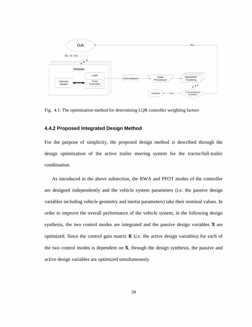
(4.3)

Fig. 4.1 shows the procedure to determine the vector .The

genetic algorithm (GA) [39] sends the randomly selected weighting factor vector to the 3-

DOF vehicle model and LQR controller constructed in Matlab. Based on the given

weighting factor vector, the controller is updated and corresponding simulation is

performed. Then a data processor calculates the performance measure of RWA for the

single lane change maneuver based on the simulation results. This set of calculated RWA

ratio is used as fitness function values. At this point, if the convergence criteria are

satisfied, the optimization terminates. Otherwise, the fitness function values are sent back

to the GA. Based on the returned fitness values, the GA produces the next generation of

design variable sets using genetic operators, e.g. selection, crossover, and mutation. This

procedure repeats until the optimized weighting factor vector is found.

Following the same procedure shown in Fig. 4.1, the weighting factor vector for the

low-speed PFOT mode, , can also be determined.

39

Vehicle

Model

RWA/Off-

Tracking

Convergence

Criteria?

GA

Cost

Function

Matlab

LQR

Solution

[q1, q2, q3]

SimulationData

Processor

No

Yes

Fig. 4.1: The optimization method for determining LQR controller weighting factors

4.4.2 Proposed Integrated Design Method

For the purpose of simplicity, the proposed design method is described through the

design optimization of the active trailer steering system for the tractor/full-trailer

combination.

As introduced in the above subsection, the RWA and PFOT modes of the controller

are designed independently and the vehicle system parameters (i.e. the passive design

variables including vehicle geometry and inertia parameters) take their nominal values. In

order to improve the overall performance of the vehicle system, in the following design

synthesis, the two control modes are integrated and the passive design variables are

optimized. Since the control gain matrix (i.e. the active design variables) for each of

the two control modes is dependent on , through the design synthesis, the passive and

active design variables are optimized simultaneously.

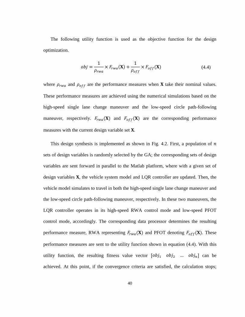
40

The following utility function is used as the objective function for the design

optimization.

(4.4)

where and are the performance measures when take their nominal values.

These performance measures are achieved using the numerical simulations based on the

high-speed single lane change maneuver and the low-speed circle path-following

maneuver, respectively. and are the corresponding performance

measures with the current design variable set .

This design synthesis is implemented as shown in Fig. 4.2. First, a population of

sets of design variables is randomly selected by the GA; the corresponding sets of design

variables are sent forward in parallel to the Matlab platform, where with a given set of

design variables , the vehicle system model and LQR controller are updated. Then, the

vehicle model simulates to travel in both the high-speed single lane change maneuver and

the low-speed circle path-following maneuver, respectively. In these two maneuvers, the

LQR controller operates in its high-speed RWA control mode and low-speed PFOT

control mode, accordingly. The corresponding data processor determines the resulting

performance measure, RWA representing and PFOT denoting . These

performance measures are sent to the utility function shown in equation (4.4). With this

utility function, the resulting fitness value vector can be

achieved. At this point, if the convergence criteria are satisfied, the calculation stops;

41

otherwise, this vector is sent back to the GA. Based on the returned fitness values

corresponding to the given sets of design variables, the GA produces the next generation

of design variable sets using selection, crossover, and mutation operators. This procedure

repeats until the optimized variable set is found.

4.5 RESULT AND DISCUSSION

In this section, the simulation results derived from the following cases are presented and

discussed: 1) baseline case, where the design variables take their nominal values and

the vehicle has no active trailer steering system; 2) control case, where the design

variables and control gain matrices take their nominal values; 3) optimal case, where

the design variables and control gain matrices take their optimized values.

4.5.1 Simulation Results of Baseline Case

In the case of numerical simulations for the baseline vehicle with non-steerable trailer

axles, the vehicle system parameters take their nominal values listed in Table B1 of

Appendix B. The simulation results for the lane change maneuver are shown in Fig. 4.3.

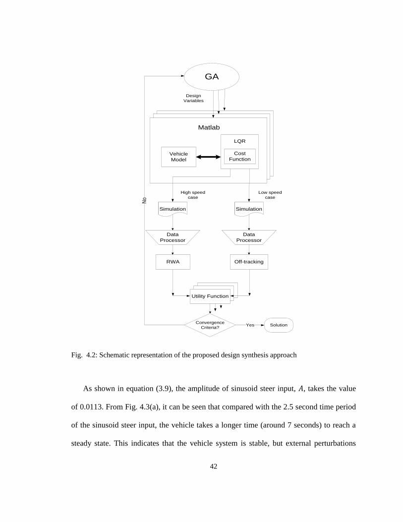
42

Vehicle

Model

RWA Off-tracking

Utility Function

Convergence

Criteria?

GA

No

Cost

Function

Matlab

LQR

High speed

case

Low speed

case

Yes Solution

Design

Variables

Simulation

Data

Processor

Simulation

Data

Processor

Fig. 4.2: Schematic representation of the proposed design synthesis approach

As shown in equation (3.9), the amplitude of sinusoid steer input, , takes the value

of 0.0113. From Fig. 4.3(a), it can be seen that compared with the 2.5 second time period

of the sinusoid steer input, the vehicle takes a longer time (around 7 seconds) to reach a

steady state. This indicates that the vehicle system is stable, but external perturbations

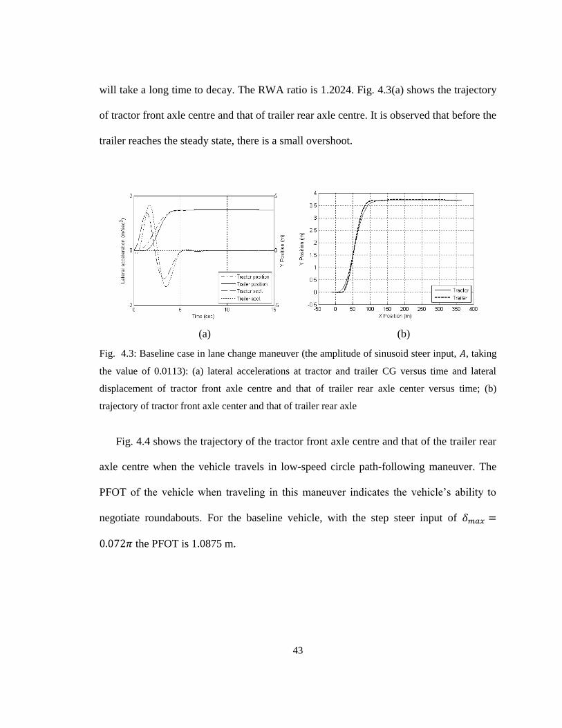
43

will take a long time to decay. The RWA ratio is 1.2024. Fig. 4.3(a) shows the trajectory

of tractor front axle centre and that of trailer rear axle centre. It is observed that before the

trailer reaches the steady state, there is a small overshoot.

(a) (b)

Fig. 4.3: Baseline case in lane change maneuver (the amplitude of sinusoid steer input, , taking

the value of 0.0113): (a) lateral accelerations at tractor and trailer CG versus time and lateral

displacement of tractor front axle centre and that of trailer rear axle center versus time; (b)

trajectory of tractor front axle center and that of trailer rear axle

Fig. 4.4 shows the trajectory of the tractor front axle centre and that of the trailer rear

axle centre when the vehicle travels in low-speed circle path-following maneuver. The

PFOT of the vehicle when traveling in this maneuver indicates the vehicle‟s ability to

negotiate roundabouts. For the baseline vehicle, with the step steer input of

the PFOT is 1.0875 m.

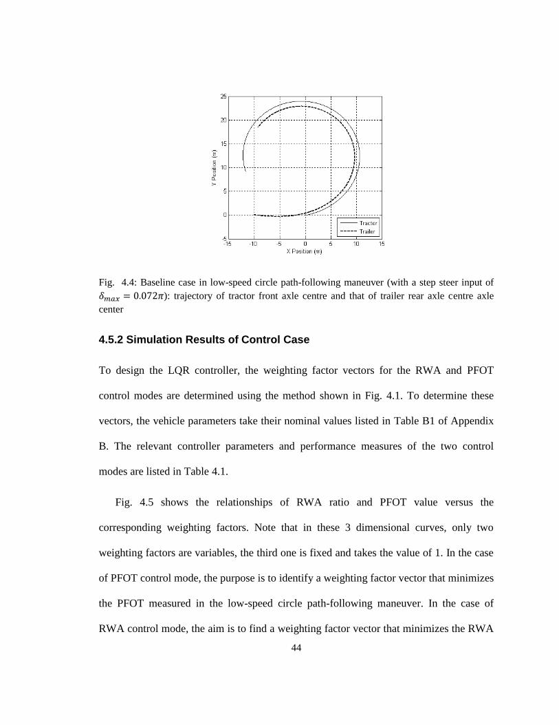
44

Fig. 4.4: Baseline case in low-speed circle path-following maneuver (with a step steer input of

): trajectory of tractor front axle centre and that of trailer rear axle centre axle

center

4.5.2 Simulation Results of Control Case

To design the LQR controller, the weighting factor vectors for the RWA and PFOT

control modes are determined using the method shown in Fig. 4.1. To determine these

vectors, the vehicle parameters take their nominal values listed in Table B1 of Appendix

B. The relevant controller parameters and performance measures of the two control

modes are listed in Table 4.1.

Fig. 4.5 shows the relationships of RWA ratio and PFOT value versus the

corresponding weighting factors. Note that in these 3 dimensional curves, only two

weighting factors are variables, the third one is fixed and takes the value of 1. In the case

of PFOT control mode, the purpose is to identify a weighting factor vector that minimizes

the PFOT measured in the low-speed circle path-following maneuver. In the case of

RWA control mode, the aim is to find a weighting factor vector that minimizes the RWA

45

ratio observed in the high-speed lane change maneuver. As shown in Figs. 4.5(a), 4.5(b)

and 4.5(c), the

Table 4.1: Resulting controller parameters and performance measures of the two control modes

RWA control mode PFOT control mode

Weighting factor

vector

Control gain

matrix

RWA ratio

(high-speed)

0.8296# 0.9782 *

PFOT

/m (low-speed)

2.2026 ** 0.8497##

* To operate the PFOT control mode in the high-speed lane change maneuver, the vehicle forward speed

dependent control gain matrix takes the value of [0.0132 -0.3793 0.0229 -0.6730].

** To operate the RWA control mode in low-speed circle path-following maneuver, the control gain matrix

takes the value of [-5.4182 0.1196 -0.7351 -0.5156].

# This RWA ratio value is the performance measure shown in equation (4.4).

## This PFOT value is the performance measure shown in equation (4.4).

performance measure of PFOT is a highly non-linear function of the weighting factors ,

, and . If the „manual‟ trial and error approach is used to find the desired weighting

factor vector, it is a tedious and time-consuming process. Moreover, this approach is not

reliable. This is also true for the case of RWA control mode, as shown in Figs. 4.5(d),

4.5(e) and 4.5(f). Using the optimization method, the „optimal‟ weighting factor vector

for both control modes can be automatically identified. The resulting weighting factor

46

vectors together with the corresponding control gain matrices are offered in Table 4.1.

With the given controller parameters and nominal vehicle system parameters, the

performance measures, RWA ratio ( rwa ) and PFOT (off

in meter), can be determined.

These performance measures are also provided in Table 4.1.

The weighting factor vectors listed in Table 4.1 and the relationships of RWA ratio

and PFOT value versus the corresponding weighting factors shown Fig. 4.5 reveal that

the RWA and PFOT control modes have different or conflicting requirements on the

weighting factors. For example, as shown in Table 4.1, for the RWA control mode,

weighting factor takes a large value of , while for the PFOT control mode,

weighting factor takes a relative small value of . Thus, the two control modes

have conflicting requirement on weighting factor . As shown in Table 4.1, for the

PFOT control mode, the low-speed PFOT is 0.8497 m, reducing by 21.87% with respect

to the baseline case, while the high-speed RWA ratio takes the value of 0.9782,

decreasing by 18.6% compared with that of the baseline case. For the RWA control

mode, RWA ratio takes the value of 0.8296, decreasing by 31.0% compared with that of

the baseline case, while the low-speed PFOT is 2.2026 m, increasing by 102.53% with

respect to the baseline case. The numerical simulation results further demonstrate the

well-known fact that for articulated heavy vehicles, the low-speed path-following and

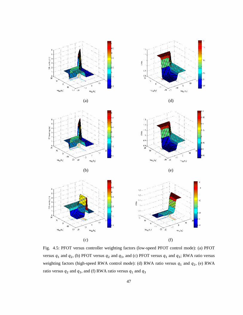
47

(a) (d)

(b) (e)

(c) (f)

Fig. 4.5: PFOT versus controller weighting factors (low-speed PFOT control mode): (a) PFOT

versus and , (b) PFOT versus and , and (c) PFOT versus and ; RWA ratio versus

weighting factors (high-speed RWA control mode): (d) RWA ratio versus and , (e) RWA

ratio versus and , and (f) RWA ratio versus and

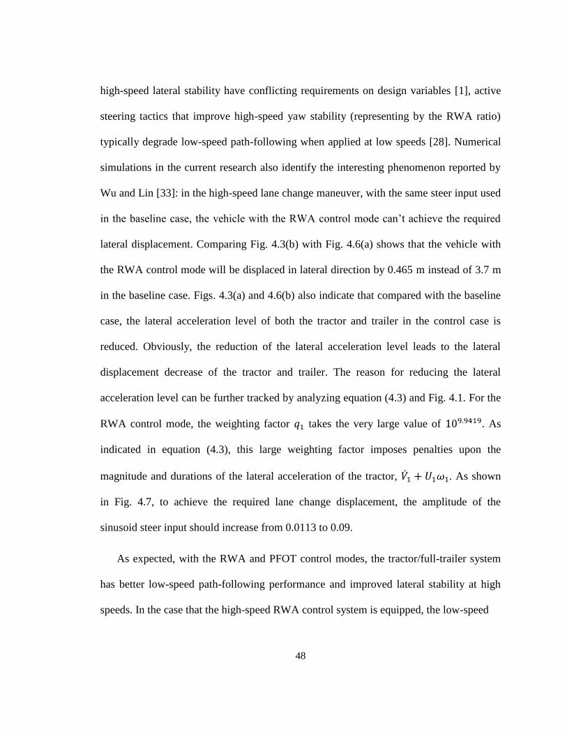
48

high-speed lateral stability have conflicting requirements on design variables [1], active

steering tactics that improve high-speed yaw stability (representing by the RWA ratio)

typically degrade low-speed path-following when applied at low speeds [28]. Numerical

simulations in the current research also identify the interesting phenomenon reported by

Wu and Lin [33]: in the high-speed lane change maneuver, with the same steer input used

in the baseline case, the vehicle with the RWA control mode can‟t achieve the required

lateral displacement. Comparing Fig. 4.3(b) with Fig. 4.6(a) shows that the vehicle with

the RWA control mode will be displaced in lateral direction by 0.465 m instead of 3.7 m

in the baseline case. Figs. 4.3(a) and 4.6(b) also indicate that compared with the baseline

case, the lateral acceleration level of both the tractor and trailer in the control case is

reduced. Obviously, the reduction of the lateral acceleration level leads to the lateral

displacement decrease of the tractor and trailer. The reason for reducing the lateral

acceleration level can be further tracked by analyzing equation (4.3) and Fig. 4.1. For the

RWA control mode, the weighting factor takes the very large value of . As

indicated in equation (4.3), this large weighting factor imposes penalties upon the

magnitude and durations of the lateral acceleration of the tractor, . As shown

in Fig. 4.7, to achieve the required lane change displacement, the amplitude of the

sinusoid steer input should increase from 0.0113 to 0.09.

As expected, with the RWA and PFOT control modes, the tractor/full-trailer system

has better low-speed path-following performance and improved lateral stability at high

speeds. In the case that the high-speed RWA control system is equipped, the low-speed

49

(a) (b)


amplitude of the sinusoid steering input, A, taking the value of 0.0113): (a) trajectory of tractor

front axle centre and that of trailer rear axle centre; (b) lateral acceleration at CG of tractor and

trailer versus time

PFOT control mode may share the same hardware, e.g. actuators, since these two control

modes have the same requirements on the control system configuration. Thus, the

introduction of the low-speed control mode may replace the conventional passive trailer

steering systems, such as self-steering and command steer systems, for improving low-

speed path-following performance. Moreover, from the vehicle design viewpoint, the

concept of low-speed control mode provides an alternative way to predict performance

envelopes for articulated vehicle low-speed path-following. However, it should be noted

that compared with traditional passive trailer steering systems, the low-speed PFOT

control mode has the disadvantage of consuming additional energy.

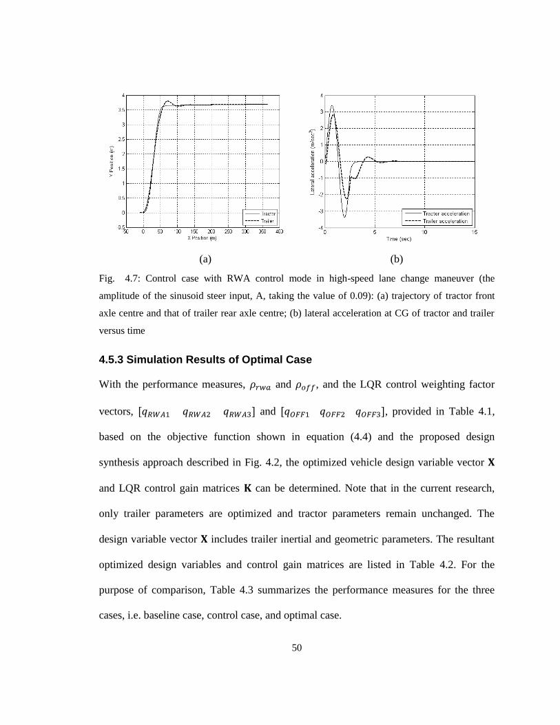
50

(a) (b)


amplitude of the sinusoid steer input, A, taking the value of 0.09): (a) trajectory of tractor front

axle centre and that of trailer rear axle centre; (b) lateral acceleration at CG of tractor and trailer

versus time

4.5.3 Simulation Results of Optimal Case

With the performance measures, and , and the LQR control weighting factor

vectors, and , provided in Table 4.1,

based on the objective function shown in equation (4.4) and the proposed design

synthesis approach described in Fig. 4.2, the optimized vehicle design variable vector

and LQR control gain matrices can be determined. Note that in the current research,

only trailer parameters are optimized and tractor parameters remain unchanged. The

design variable vector includes trailer inertial and geometric parameters. The resultant

optimized design variables and control gain matrices are listed in Table 4.2. For the

purpose of comparison, Table 4.3 summarizes the performance measures for the three

cases, i.e. baseline case, control case, and optimal case.

51

Table 4.2: Optimized design variables and controller gain matrices

Design

variables

Nominal values Upper

bounds

Lower

bounds

Optimized variables

(kg) 5460 6006 4914 4914.1

(kg m2) 12540 13794 11286 12269

(m) 2.44 2.684 2.196 2.1960

(m) 1.68 1.848 1.512 1.512

(m) 1.37 1.507 1.233 1.233

RWA control

gain

[0.0995 -1.1379

-0.0334 -0.05156]

[0.0960 -1.0925

-0.0559 -0.5913]

PFOT control

gain

[-0.7043 3.6369

-2.5142 -0.5098]

[-0.7582 3.7544

-2.6505 -0.5632]

Fig. 4.9 shows the simulation results of the optimized vehicle under the high-speed

lane change maneuver with the amplitude of the sinusoid steering input taking the

value of 0.09. Fig. 4.8(a) illustrates that in the optimal case, the tractor and trailer first

reach the lateral displacement of 3.7 m at 2.56 s and 2.9 s, respectively, while in the

baseline case shown in Fig. 4.3(a), the tractor and trailer first achieve this lateral

displacement at 5.9 s and 6.4 s, correspondingly. Fig. 4.8(b) demonstrates that in the

optimal case, the tractor is able to complete the lane change around a longitudinal

distance of 65 m, while in the baseline case shown in Fig. 4.3(b), the tractor requires a

distance of 110 m. The trailer trajectories shown in Figs. 4.3(b) and 4.8(b) indicate that

compared with the baseline case, the trailer of the optimized vehicle experiences a larger

overshoot. Thus, compared with the baseline vehicle, the optimized vehicle responds the

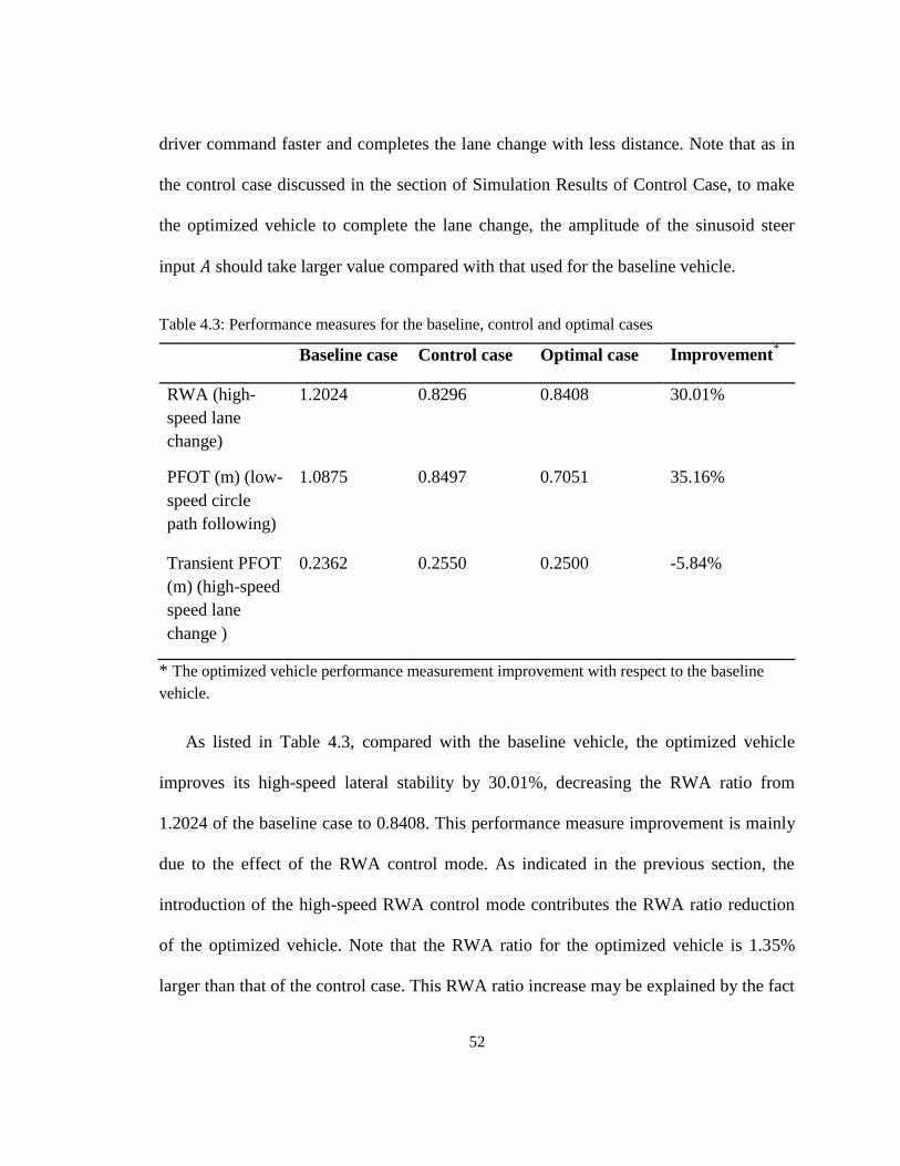
52

driver command faster and completes the lane change with less distance. Note that as in

the control case discussed in the section of Simulation Results of Control Case, to make

the optimized vehicle to complete the lane change, the amplitude of the sinusoid steer

input should take larger value compared with that used for the baseline vehicle.

Table 4.3: Performance measures for the baseline, control and optimal cases

Baseline case Control case Optimal case Improvement*

RWA (high-

speed lane

change)

1.2024 0.8296 0.8408 30.01%

PFOT (m) (low-

speed circle

path following)

1.0875 0.8497 0.7051 35.16%

Transient PFOT

(m) (high-speed

speed lane

change )

0.2362 0.2550 0.2500 -5.84%

* The optimized vehicle performance measurement improvement with respect to the baseline

vehicle.

As listed in Table 4.3, compared with the baseline vehicle, the optimized vehicle

improves its high-speed lateral stability by 30.01%, decreasing the RWA ratio from

1.2024 of the baseline case to 0.8408. This performance measure improvement is mainly

due to the effect of the RWA control mode. As indicated in the previous section, the

introduction of the high-speed RWA control mode contributes the RWA ratio reduction

of the optimized vehicle. Note that the RWA ratio for the optimized vehicle is 1.35%

larger than that of the control case. This RWA ratio increase may be explained by the fact

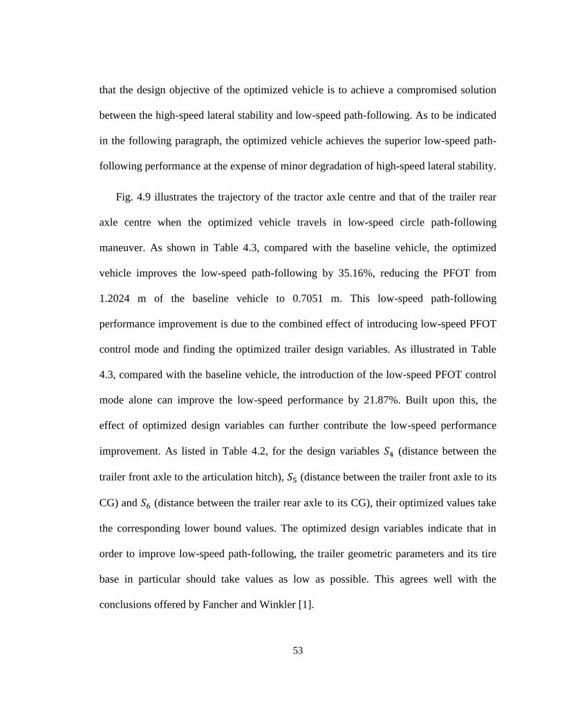
53

that the design objective of the optimized vehicle is to achieve a compromised solution

between the high-speed lateral stability and low-speed path-following. As to be indicated

in the following paragraph, the optimized vehicle achieves the superior low-speed path-

following performance at the expense of minor degradation of high-speed lateral stability.

Fig. 4.9 illustrates the trajectory of the tractor axle centre and that of the trailer rear

axle centre when the optimized vehicle travels in low-speed circle path-following

maneuver. As shown in Table 4.3, compared with the baseline vehicle, the optimized

vehicle improves the low-speed path-following by 35.16%, reducing the PFOT from

1.2024 m of the baseline vehicle to 0.7051 m. This low-speed path-following

performance improvement is due to the combined effect of introducing low-speed PFOT

control mode and finding the optimized trailer design variables. As illustrated in Table

4.3, compared with the baseline vehicle, the introduction of the low-speed PFOT control

mode alone can improve the low-speed performance by 21.87%. Built upon this, the

effect of optimized design variables can further contribute the low-speed performance

improvement. As listed in Table 4.2, for the design variables (distance between the

trailer front axle to the articulation hitch), (distance between the trailer front axle to its

CG) and (distance between the trailer rear axle to its CG), their optimized values take

the corresponding lower bound values. The optimized design variables indicate that in

order to improve low-speed path-following, the trailer geometric parameters and its tire

base in particular should take values as low as possible. This agrees well with the

conclusions offered by Fancher and Winkler [1].

54

Table 4.3 also offers the transient PFOT values for the three cases in the high-speed

lane change maneuver. The optimal and control cases have higher levels of transient

PFOT

(a) (b)

Fig. 4.8: Optimal case in high-speed lane change maneuver (the amplitude of the sinusoid steer

input, , taking the value of 0.09): (a) lateral acceleration at CG of tractor and trailer versus time

and lateral displacement of tractor front axle centre and that of trailer rear axle centre versus time;

(b) trajectory of tractor front axle centre and that of trailer rear axle centre

than that of the baseline case. A good indication of the relative performance of each case

can be observed in the high-speed lane change paths shown in Figs. 4.3(b), 4.7(a) and

4.8(b). The worst performing case is the control case with the RWA control mode. The

transient PFOT value in the control case is 8.0% higher than that of the baseline case.

Compared with the control case, the optimized vehicle has less transient PFOT value,

decreasing from 0.255 m of the control case to 0.25 m. In all cases, the level of transient

PFOT is well below the performance measure of 0.8 m proposed by Australia‟s National

Road Transport Commission [32].

55

Fig. 4.9: Optimal case in low-speed circle path-following maneuver (with a step steer input of

): trajectory of tractor front axle centre and that of trailer rear axle centre

Among the three cases listed in Table 4.3, the optimized vehicle has the best overall

performance in terms of high-speed lane change RWA ratio, low-speed PFOT value, and

high-speed lane change transient PFOT. This superior overall performance of the

optimized vehicle is due to the integrated design optimization of the trailer‟s inertial and

geometric parameters as well as the active trailer steering system with the RWA and

PFOT control modes.

4.6 CONCLUSIONS

This chapter proposes the two loop design (TLD) method for active trailer steering (ATS)

systems of articulated heavy vehicles (AHVs). To improve the overall performance of

AHVs, the passive vehicle design variables, such as trailer geometric and inertial

parameters, and the active design variables of ATS systems, e.g. the control gain matrices

56

of the optimal controller based on the linear quadratic regular (LQR) theory, can be

optimized simultaneously. In order to coordinate the conflicting performance

requirements of the low-speed path-following and the high-speed lateral stability of

AHVs, the LQR controller has two operational modes: the low-speed PFOT (Path-

Following Off-Tracking) control mode is designed in such a way that in a low-speed

circle path-following maneuver, the PFOT of the AHV is minimized; the high-speed

RWA control mode is developed following the idea that the vehicle system is optimized

to make the Rear-Ward Amplification (RWA) ratio as small as possible in the high-speed

single lane change maneuver. In the design of the LQR controller, the weighting factor

vectors are determined using an optimization method instead of the conventional trial and

error approaches.

To demonstrate the feasibility and effectiveness of the proposed design method, it is

applied to the design of a front trailer axle active steering system for a tractor/full-trailer

combination based on a 3 degree-of-freedom (DOF) linear yaw plane model. The active

steering control strategy is explained from a vehicle dynamic viewpoint. An

instrumentation arrangement for implementing this control is recommended. Simulation

results illustrate that in comparison to the baseline vehicle, the one derived from the

design synthesis approach decreases the low-speed PFOT by 35.16% and reduces the

high-speed RWA ratio by 30.01%. The proposed approach may be used for identifying

desired design variables and predicting performance envelopes in the early design stages

of AHVs with ATS systems.

57

Chapter 5

SINGLE DESIGN LOOP METHOD FOR THE

DESIGN OF AHVS WITH ATS SYSTEMS

5.1 INTRODUCTION

This chapter presents an automated design synthesis approach, called a single loop (SDL)

method, for articulated heavy vehicles (AHVs) with active trailer steering (ATS) systems.

AHVs have poor maneuverability when traveling at low speeds. Moreover, AHVs exhibit

unstable motion modes at high speeds. To address the problem of maneuverability,

„passive‟ trailer steering systems have been developed. These systems improve low-speed

performance, but feature with low lateral stability at high speeds. Some ATS systems

have been proposed to improve high-speed lateral stability. However, these systems

typically degrade maneuverability when applied at low speeds. To tackle this conflicting

design problem, a systematic method is proposed for the design of AHVs with ATS

systems. This new design method has the following features: the optimal active design

variables of the ATS systems and the optimal passive design variables of the vehicle are

identified in a single design loop; in the design process, to evaluate the vehicle

performance measures, a driver model is introduced and it „drives‟ the vehicle model

based on the well-defined testing specifications. Through the design optimization of an

ATS system for an AHV with a tractor and a full trailer, this SDL method is compared

58

against the two design loop (TDL) method, presented in the previous chapter. The

benchmark investigation shows that the former can determine better trade-off design

solutions than those derived by the latter. This SDL method provides an effective

approach to automatically implement the design synthesis of AHVs with ATS systems.

The rest of this chapter is organized as follows. Section 5.2 introduces the driver

model and the test maneuver emulated for evaluating the AHV performance at low and

high speeds. Moreover, the construction of the LQR controller for ATS systems is

outlined in the same section. The proposed SDL method is presented in Section 5.3.

Section 5.4 compares the design results derived from the SDL approach against those

based on the TDL method. Finally, conclusions are drawn in Section 5.5.


5.2.1 Vehicle Model

The proposed SDL method is examined and evaluated by applying it in design of a

tractor/full-trailer system as used in the previous chapter. The details of the vehicle model

(called as Model-1), utilized in this chapter to determine the directional performance

measure of the vehicle system, is described in Subsection 3.2.1.

5.2.2 Maneuvers emulated

Two test maneuvers, i.e. the 90-degree intersection turn [32] and the single-lane change

specified in SAE J2179 [35], are widely accepted for measuring low-speed PFOT and

59

high-speed RWA ratio of AHVs, respectively. In each of the maneuvers, the vehicle

tested is required to follow a precisely prescribed path at a specified speed and the diver

should continuously monitor and adjust steering actions accordingly. In the current

research, the recommended single lane change test procedure has been simulated for

determining the high-speed RWA ratio. In this simulation, the vehicle is traveling at the

speed of 88 km/h along a straight path section. Then, a sudden lane change is conducted.

The lateral displacement of the vehicle in the lane change is 1.46 m. The maneuver

emulated during the design process for measuring low-speed PFOT is based on the 90-

degree intersection turn test procedure. In this case, the center of tractor front axle is

required to travel along a specified path. The vehicle travels at the constant speed of 4

km/h. Moreover, to compare the low-speed PFOT of the optimal designs against that of

baseline vehicles, the test maneuver similar to the 360-degree roundabout defined in the

United Kingdom‟s Road Vehicles Regulation [32] has also emulated in the research.

5.2.3 Driver Model

The driver model developed in the research is based on a modified PID control technique.

The driver model is to „drive‟ the vehicle along the prescribed path. The vehicle steering

angle correction is made through the PID control of the vehicle position error. The

position error is defined as the distance from the tractor‟s front axle center to the desired

point on the specified path measured along the corresponding radius of curvature.

As shown in Fig. 5.1, the prescribed path is defined by a series of point, ,

, in the global coordinate system . The position vectors of the tractor

60

CG, tractor front axle center and the target point on the path are denoted as , , and ,

respectively. In the global coordinate system, these vectors are expressed as

X

Y

r

frdr

1S

3S2S

5S

6S

4Sdfr

*

nX1nX2nX

1nX

p

fX

Fig. 5.1: Geometry representation of vehicle and prescribed path

(5.1a)

(5.1b)

(5.1c)

where and are unit vectors in and directions, respectively. If the initial position of

tractor CG and the angle swept from the longitudinal axis of the tractor to the -axis are

and , respectively, the corresponding position of the tractor front axle center

( ) can be determined as

61

(5.2a)

(5.2b)

In the simulation of the high speed single lane change test maneuver, at an arbitrary time

instant , the vehicle position error, is defined as follows. Assume that at this

instant, the position of the tractor front axle center is , and on the prescribed

path the two adjoining points close to the tractor front axle center are and

If point is selected as the target point on the

prescribed path. The vehicle position error is defined as the distance measured from

the point to the straight line connecting the points and

. In the simulations of the 90-degree intersection turn and 360-degree roundabout

test maneuvers, the vehicle position error is defined as the distance between the

point and the corresponding point on the prescribed path measured along

the radius of curvature.

The desired vehicle heading direction can be represented with the position vector

defined by

(5.3)

The angle swept from vector to axis is denoted as . The pseudo vehicle

steering angle can be determined by

(5.4)

62

where is the angle swept from the longitudinal axis of the tractor to the -axis at the

time instant . The vehicle steering angle correction at this instant is defined as

(5.5)

where is a control variable determined using the following PID control of the

vehicle position error.

(5.6)

In equation (5.6), , and represent the proportional, integral and derivative

controller gains, respectively.

With the vehicle steering angle input , the differential equation of the vehicle

model, as shown in equation (3.3), can be solved in the time interval from to .

Tractor lateral velocity and yaw rate can be determined. If the

time increment is very small, the vehicle heading angel increment can be

calculated by

(5.7)

Note that the direction of yaw rate and that of vehicle heading angle are opposite.

Thus, the resulting heading angle at the time instant is

(5.8)

63

Over the time interval , the position variation of the tractor CG can be determined

using the constant vehicle forward speed and the instantaneous vehicle lateral speed

.

(5.9a)

(5.9b)

Then at the time instant , the position of tractor CG and its front axle center can

be determined by

(5.10a)

(5.10b)

and

(5.11a)

(5.11b)

respectively. Following the same procedure described above, the vehicle steering angle

input at the time instant can be determined.

To validate the developed driver model, it has been integrated with the 3-DOF vehicle

model and the numerical simulations for the low-speed 90-degree intersection turn and

high-speed single lane change test maneuvers have been conducted. Note that in these

simulations, the vehicle system parameters take their nominal values provided in Table

B1 of Appendix B. Fig. 5.2 shows the simulated trajectory of the tractor front axle center

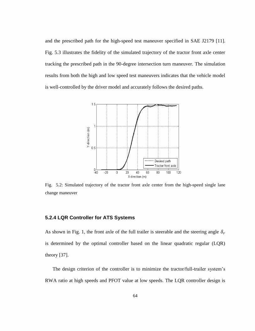
64

and the prescribed path for the high-speed test maneuver specified in SAE J2179 [11].

Fig. 5.3 illustrates the fidelity of the simulated trajectory of the tractor front axle center

tracking the prescribed path in the 90-degree intersection turn maneuver. The simulation

results from both the high and low speed test maneuvers indicates that the vehicle model

is well-controlled by the driver model and accurately follows the desired paths.

Fig. 5.2: Simulated trajectory of the tractor front axle center from the high-speed single lane

change maneuver

5.2.4 LQR Controller for ATS Systems

As shown in Fig. 1, the front axle of the full trailer is steerable and the steering angle

is determined by the optimal controller based on the linear quadratic regular (LQR)

theory [37].

The design criterion of the controller is to minimize the tractor/full-trailer system‟s

RWA ratio at high speeds and PFOT value at low speeds. The LQR controller design is

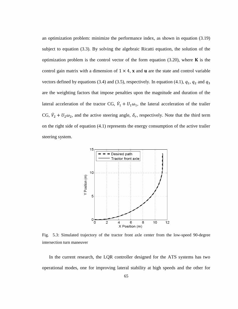
65

an optimization problem: minimize the performance index, as shown in equation (3.19)

subject to equation (3.3). By solving the algebraic Ricatti equation, the solution of the

optimization problem is the control vector of the form equation (3.20), where is the

control gain matrix with a dimension of , and are the state and control variable

vectors defined by equations (3.4) and (3.5), respectively. In equation (4.1), , and

are the weighting factors that impose penalties upon the magnitude and duration of the

lateral acceleration of the tractor CG, , the lateral acceleration of the trailer

CG, , and the active steering angle, , respectively. Note that the third term

on the right side of equation (4.1) represents the energy consumption of the active trailer

steering system.

Fig. 5.3: Simulated trajectory of the tractor front axle center from the low-speed 90-degree

intersection turn maneuver

In the current research, the LQR controller designed for the ATS systems has two

operational modes, one for improving lateral stability at high speeds and the other for

66

enhancing path-following at low speeds. Based on equation (4.1), for these two control

modes, the weighting factor vectors are denoted as and

, respectively. Accordingly, the control gain vectors based on

equation (3.5) are represented as and .

5.3 AUTOMATED DESIGN SYNTHESIS APPROACH

Fig. 5.5 shows the preliminary framework of the proposed automated design synthesis

approach for AHVs with ATS systems. The design optimization of AHVs is implemented

using a genetic algorithm (GA). The AHV model may be generated using multibody

dynamic programs, e.g. ADAMS and TruckSim. The ATS controller based on LQR

technique and the driver model can be constructed in Matlab. Then, the combined vehicle

model, ATS controller and driver model are optimized simultaneously using the GA.

As shown in Fig. 5.5, a population of n sets of design variables evaluated by the GA

is sent forward in parallel to the AHV model, ATS controller and driver model. For a

given design variable set , it includes , and . Note that in the current

research represents passive vehicle system parameters, such as the trailer geometric

and inertia parameters, denotes , and stands for

. With this set of design variables, the vehicle system model

is generated, and the LQR controller and driver model are constructed. Then, the driver

model will „drive‟ the vehicle model in both the high-speed single lane change maneuver

and the low-speed 90-degree interaction turn maneuver, respectively. In these two

67

maneuvers, the LQR controller operates in its high-speed RWA and low-speed PFOT

control modes, accordingly. The corresponding data processor determines the resulting

performance measure, RWA representing and PFOT denoting

. These performance measures are to be used for the cost function

evaluation in the form of the following utility function.

(5.12)

where and denotes RWA ratio and PFOT value of the baseline vehicle for

high speed lane change and low speed turning maneuvers, respectively, and are

two constants. Corresponding to the n sets of design variables, the resulting fitness value

vector can be achieved. At this point, if the convergence

criteria are satisfied, the calculation terminates; otherwise, this vector is sent back to the

GA. Based on the returned fitness values corresponding to the given sets of design

variables, the GA produces the next generation of design variable sets using selection,

crossover, and mutation operators. This procedure repeats until the optimized variable set

is found.

With the above automated design synthesis approach, all optimal design variables,

including the weighting factors for constructing the LQR controller, LQR controller

gains, and passive vehicle system design variables, can be identified in a single design

loop (SDL). Compared with the two design loop (TDL) method recommended in Ref.

68

[12], the proposed SDL approach is more suitable for automated design process of

AHVs.

5.4 RESULTS AND DISCUSSION

In this section, the simulation results from the SDL method are discussed and compared

with those from the TDL approach reported in Ref. [12]. To make the results from the

two design methods comparable, in both cases, the driver model has been incorporated in

the simulated test maneuvers. Both design methods have been applied to the design

synthesis of an AHV with ATS systems using the 3-DOF vehicle model. The baseline

vehicle system parameters are provided in Table B1 of Appendix B. In the case of TDL

method, in the first design loop, the design variables are the weighting factor vectors

and , which are used to constructed

the LQR controllers for the RWA and PFOT control modes. In the second design loop,

the design variables consists of the trailer geometric and inertia parameters, including

, , , and , and controller gain vectors and for the RWA and

PFOT control modes, respectively. In the case of SDL method, the optimized values of

all the above design variables are found in a single design loop.

With an operation of the SDL method shown in Fig. 5.4, the optimized values of the

design variables have been found and they are listed in Table 5.1 together with the

nominal values of the passive design variables.

69

High speed case Low speed case

Mulitbody

Vehicle

Model

RWA PFOT

Utility

Function

Convergence

Criteria?

GA

No

Matlab

Yes Solution

Design

Variables

Simulation

Data

Processor

Simulation

Data

Processor

Driver Model

SYSXRWAX[

Cost Function

LQR

]PFOTX

Fig. 5.4: Schematic representation of the automated design synthesis approach

In the SDL and baseline design cases, the selected resulting vehicle dynamic

responses are illustrated in Figs. 5.5, 5.6, 5.7 and 5.8. Note that in the baseline vehicle

case, the vehicle system parameters take their nominal values offered in Appendix B and

the trailer is non-steerable. Fig. 5.5 shows the time history of the lateral accelerations of

the tractor and trailer CG in the high speed single lane change maneuver for both the

70

baseline and SDL designs. Due to the RWA control mode of the ATS system and the

optimal passive design variables derived from the SDL method, the RWA ratio decreases

by 48.67%, changing from the baseline value of 1.573 to 0.8074. The drop of the RWA

ratio will greatly improve the high-speed lateral stability to the resulting design.

Fig. 5.6 provides useful simulation results for investigating whether the trailer can

follow the tractor‟s trajectory accurately in the high-speed lane change maneuver.

Compared with the baseline vehicle, in the case of the SDL design, the trailer follows the

tractor‟s path more accurately with the maximum transient PFOT of 0.3048 m,

decreasing 5.78% from the corresponding baseline value of 0.3235 m. Results shown in

Figs 5.5 and 5.6 imply that with respect to the baseline design, in the case of the SDL

design, the vehicle system has higher lateral stability and the trailer can more accurately

follow the tractor‟s path in high-speed obstacle avoidance situations.

With the simulation results shown in Fig. 5.7, the SDL design‟s low-speed

maneuverability can be examined and evaluated. Fig. 5.7(a) offers the simulation result

of the baseline design, illustrating the trajectory of the tractor‟s front axle center and that

of the trailer‟s rear axle center in the low-speed 90-degree intersection turn test

maneuver. Fig. 5.7(b) shows the corresponding simulation result for the SDL design. A

close observation of the simulation results reveals that compared with the baseline

design, in the case of the SDL design, the trailer can track the tractor trajectory more

closely. For the SDL design, the maximum PFOT (Path-Following Off-Tracking) value

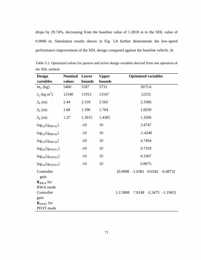
71

drops by 29.74%, decreasing from the baseline value of 1.2818 m to the SDL value of

0.9006 m. Simulation results shown in Fig. 5.8 further demonstrate the low-speed

performance improvement of the SDL design compared against the baseline vehicle. In

Table 5.1: Optimized values for passive and active design variables derived from one operation of

the SDL method

Design

variables

Nominal

values

Lower

bounds

Upper

bounds

Optimized variables

(kg) 5460 5187 5733 5675.6

(kg m2) 12540 11913 13167 12255

(m) 2.44 2.318 2.562 2.3366

(m) 1.68 1.596 1.764 1.6039

(m) 1.37 1.3015 1.4385 1.3506

-10 10 3.4747

-10 10 -1.4240

-10 10 4.7494

-10 10 0.7329

-10 10 0.3307

-10 10 0.8975

Controller

gain

for

RWA mode

[0.0908 -1.0381 -0.0342 -0.4873]

Controller

gain

for

PFOT mode

[-2.5808 7.8148 -5.3475 -1.1963]

72

(a) (b)

Fig. 5.5: Lateral acceleration at CG of tractor and trailer versus time (results achieved in the

simulated high-speed lane change maneuver): (a) baseline design case; (b) SDL design case

(a) (b)

Fig. 5.6: Trajectory of track front axle center and that of trailer rear axle center (results achieved

in the simulated high-speed lane change maneuver): (a) baseline design case; (b) SDL design case

the case of the baseline design, Fig. 5.8(a) offers the simulation result of the trajectory of

the tractor‟s front axle center and that of the trailer‟s rear axle center in the low-speed

360-degree roundabout test maneuver. Fig. 5.8(b) provides the corresponding result for

the SDL design. The simulation results offered in Fig. 5.8 indicate that the steady state

PFOT value of the SDL design is 3.56% lower than that of the baseline design,

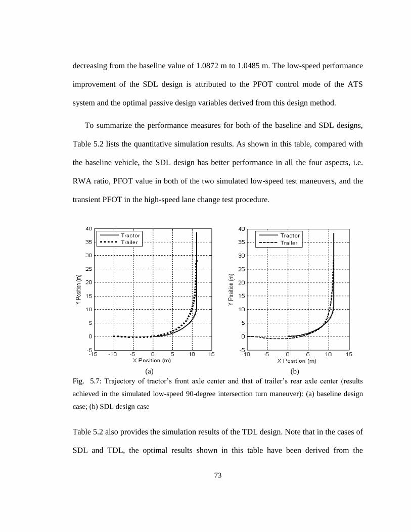
73

decreasing from the baseline value of 1.0872 m to 1.0485 m. The low-speed performance

improvement of the SDL design is attributed to the PFOT control mode of the ATS

system and the optimal passive design variables derived from this design method.

To summarize the performance measures for both of the baseline and SDL designs,

Table 5.2 lists the quantitative simulation results. As shown in this table, compared with

the baseline vehicle, the SDL design has better performance in all the four aspects, i.e.

RWA ratio, PFOT value in both of the two simulated low-speed test maneuvers, and the

transient PFOT in the high-speed lane change test procedure.

(a) (b)


achieved in the simulated low-speed 90-degree intersection turn maneuver): (a) baseline design

case; (b) SDL design case

Table 5.2 also provides the simulation results of the TDL design. Note that in the cases of

SDL and TDL, the optimal results shown in this table have been derived from the

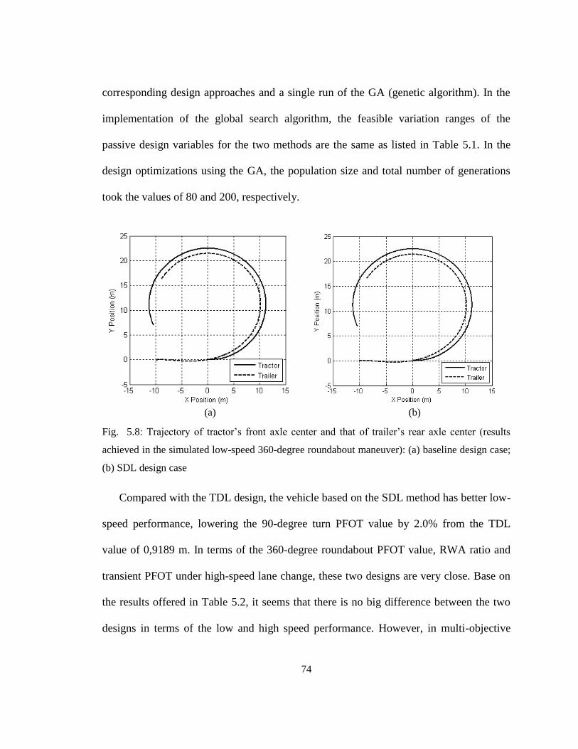
74

corresponding design approaches and a single run of the GA (genetic algorithm). In the

implementation of the global search algorithm, the feasible variation ranges of the

passive design variables for the two methods are the same as listed in Table 5.1. In the

design optimizations using the GA, the population size and total number of generations

took the values of 80 and 200, respectively.

(a) (b)


achieved in the simulated low-speed 360-degree roundabout maneuver): (a) baseline design case;

(b) SDL design case

Compared with the TDL design, the vehicle based on the SDL method has better low-

speed performance, lowering the 90-degree turn PFOT value by 2.0% from the TDL

value of 0,9189 m. In terms of the 360-degree roundabout PFOT value, RWA ratio and

transient PFOT under high-speed lane change, these two designs are very close. Base on

the results offered in Table 5.2, it seems that there is no big difference between the two

designs in terms of the low and high speed performance. However, in multi-objective

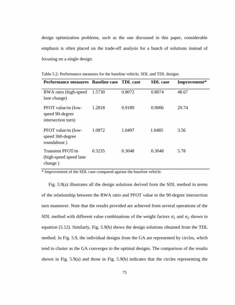
75

design optimization problems, such as the one discussed in this paper, considerable

emphasis is often placed on the trade-off analysis for a bunch of solutions instead of

focusing on a single design.

Table 5.2: Performance measures for the baseline vehicle, SDL and TDL designs

Performance measures Baseline case TDL case SDL case Improvement*

RWA ratio (high-speed

lane change)

1.5730 0.8072 0.8074 48.67

PFOT value/m (low-

speed 90-degree

intersection turn)

1.2818 0.9189 0.9006 29.74

PFOT value/m (low-

speed 360-degree

roundabout )

1.0872 1.0497 1.0485 3.56

Transient PFOT/m

(high-speed speed lane

change )

0.3235 0.3048 0.3048 5.78

* Improvement of the SDL case compared against the baseline vehicle.

Fig. 5.9(a) illustrates all the design solutions derived from the SDL method in terms

of the relationship between the RWA ratio and PFOT value in the 90-degree intersection

turn maneuver. Note that the results provided are achieved from several operations of the

SDL method with different value combinations of the weight factors and shown in

equation (5.12). Similarly, Fig. 5.9(b) shows the design solutions obtained from the TDL

method. In Fig. 5.9, the individual designs from the GA are represented by circles, which

tend to cluster as the GA converges to the optimal designs. The comparison of the results

shown in Fig. 5.9(a) and those in Fig. 5.9(b) indicates that the circles representing the

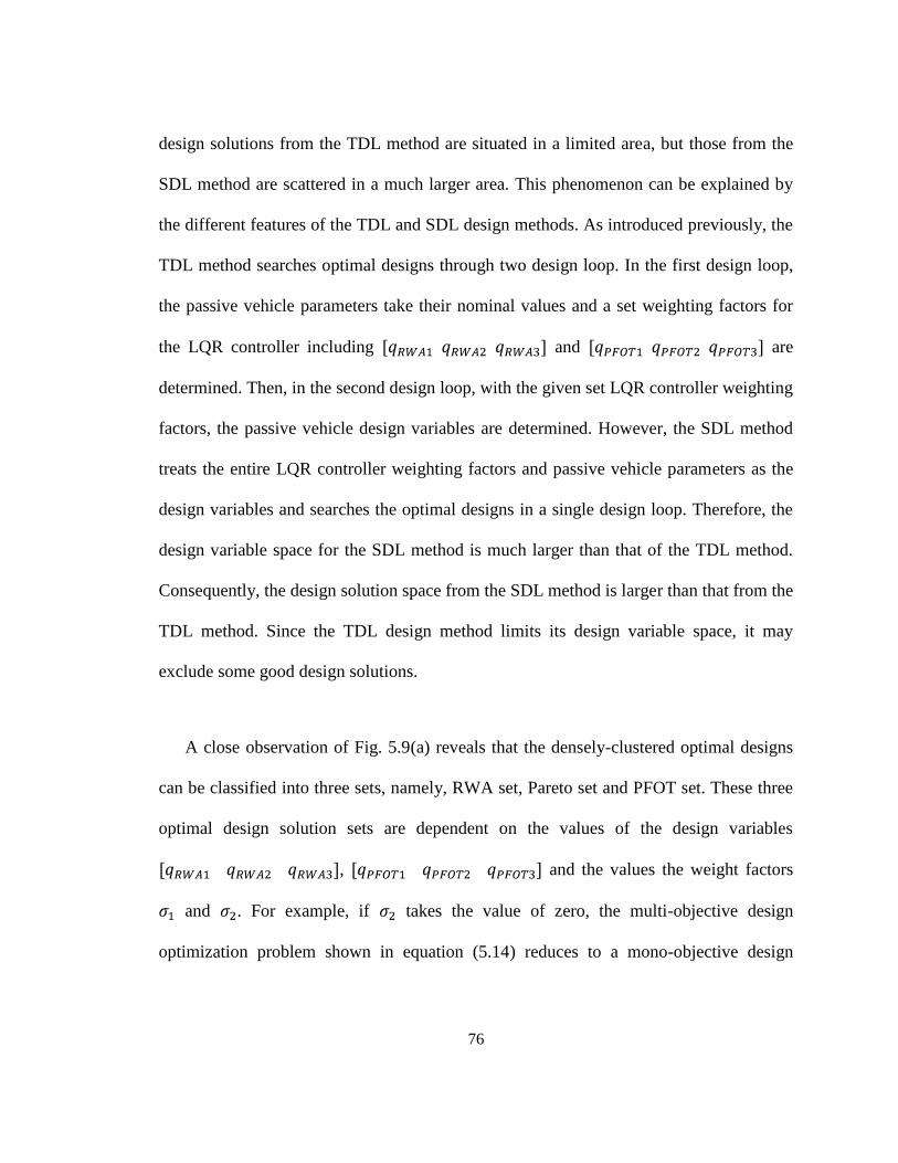
76

design solutions from the TDL method are situated in a limited area, but those from the

SDL method are scattered in a much larger area. This phenomenon can be explained by

the different features of the TDL and SDL design methods. As introduced previously, the

TDL method searches optimal designs through two design loop. In the first design loop,

the passive vehicle parameters take their nominal values and a set weighting factors for

the LQR controller including and are

determined. Then, in the second design loop, with the given set LQR controller weighting

factors, the passive vehicle design variables are determined. However, the SDL method

treats the entire LQR controller weighting factors and passive vehicle parameters as the

design variables and searches the optimal designs in a single design loop. Therefore, the

design variable space for the SDL method is much larger than that of the TDL method.

Consequently, the design solution space from the SDL method is larger than that from the

TDL method. Since the TDL design method limits its design variable space, it may

exclude some good design solutions.

A close observation of Fig. 5.9(a) reveals that the densely-clustered optimal designs

can be classified into three sets, namely, RWA set, Pareto set and PFOT set. These three

optimal design solution sets are dependent on the values of the design variables

, and the values the weight factors

and . For example, if takes the value of zero, the multi-objective design

optimization problem shown in equation (5.14) reduces to a mono-objective design

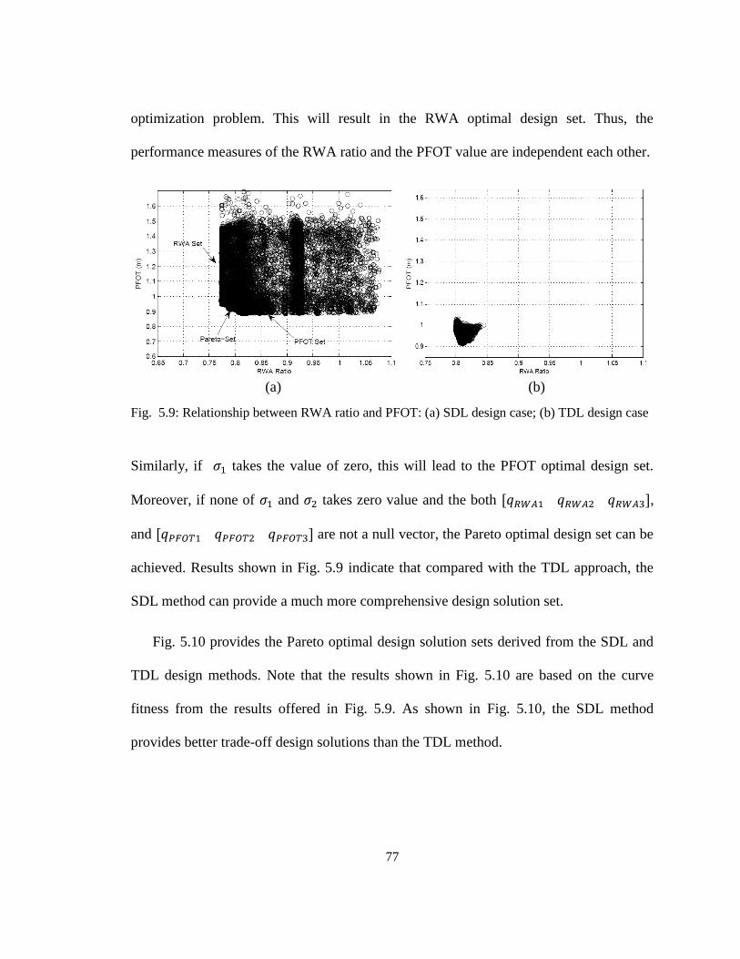
77

optimization problem. This will result in the RWA optimal design set. Thus, the

performance measures of the RWA ratio and the PFOT value are independent each other.

(a) (b)

Fig. 5.9: Relationship between RWA ratio and PFOT: (a) SDL design case; (b) TDL design case

Similarly, if takes the value of zero, this will lead to the PFOT optimal design set.

Moreover, if none of and takes zero value and the both ,

and are not a null vector, the Pareto optimal design set can be

achieved. Results shown in Fig. 5.9 indicate that compared with the TDL approach, the

SDL method can provide a much more comprehensive design solution set.

Fig. 5.10 provides the Pareto optimal design solution sets derived from the SDL and

TDL design methods. Note that the results shown in Fig. 5.10 are based on the curve

fitness from the results offered in Fig. 5.9. As shown in Fig. 5.10, the SDL method

provides better trade-off design solutions than the TDL method.

78

Fig. 5.10: Trade-off design solutions derived from SDL method (solid line) and TDL method

(dashed line)

5.5 CONCLUSIONS

This chapter presents an automated design synthesis approach, called Single Design Loop

(SDL) method, for the design of articulated heavy vehicles (AHVs) with active trailer

steering (ATS) systems. The proposed design method has the following distinguished

features: 1) the optimal active design variables of the ATS systems and the optimal

passive vehicle system design variables are searched in a single design loop; 2) in the

design process, to evaluate the vehicle performance measures, a driver model is

introduced and it „drives‟ the vehicle model based on the well-defined testing

specifications. The ATS systems derived from this design method have two operational

modes, one for improving the lateral stability at high speeds and the other for enhancing

the path-following at low speeds. With the suggested combination of multibody vehicle

79

modeling/simulation technique and optimization algorithms, the SDL method is suitable

for the automated design synthesis of AHVs with ATS systems.

The proposed SDL method has been applied to the design of an AHVs with ATS

systems using a 3 degrees of freedom vehicle model. An optimal design derived from this

method is compared with the baseline vehicle. Numerical simulation results show that the

optimal design is superior to the baseline vehicle in the performance measures of high-

speed lateral stability and low-speed path-following. The optimal design reduces the

RWA (Rear-Ward Amplification) ratio in an obstacle avoidance lane change by 48.67 %

from the baseline value, decreases the PFOT (Path-Following Off-Tracking) by 29.74 %

from the baseline value.

Compared with the two design loop (TDL) design method reported in Ref. [12], the

SDL approach searches solutions in a much larger design space and consequently it

provides a more comprehensive set of optimal designs. This comprehensive set of

optimal designs can be classified into three subsets, namely, RWA set for improving

high-speed lateral stability, PFOT set for enhancing low-speed maneuverability, and

Pareto set for optimal trade-off coordination between the high-speed stability and low-

speed maneuverability. Simulation results illustrate that for the given design application,

the SDL method offers better trade-off design solutions than the TDL approach. The

proposed SDL method may be used for identifying desired design variables and

predicting performance envelops in the early design stages of AHVs with ATS systems.

80

Chapter 6

A COMPOUND LATERAL POSITION

DEVIATION PREVIEW CONTROLLER

6.1 INTRODUCTION

An optimal preview controller, called compound lateral position deviation preview

(CLPDP) controller, is designed for active trailer steering (ATS) systems to improve

high-speed stability of articulated heavy vehicles (AHVs). The main reason of many

recently reported highway accidents is due to AHVs‟ unstable motion modes, including

jack-knifing and rollover. To prevent these unstable motion modes, the optimal

controller, namely the compound lateral position deviation preview controller (CLPDP)

is proposed to control the steering of the front and rear axle tires of the trailing unit of a

tractor/full-trailer combination. The corrective steering angle of the trailer front axle tires

is determined using the preview information of the lateral position deviation of the

trajectory of the axle center from that of the tractor front axle center. In turn, the steering

angle of the trailer rear axle tires is calculated considering the lateral position deviation of

the trajectory of the axle center from that of the trailer front axle. The linear quadratic

regular technique is applied to the design of the proposed preview control scheme in the

continuous time domain.

81

The rest of the chapter is organized as follows. Section 6.2 states the vehicle model

and maneuver used in the design of the CLPDP controller for the ATS system of the

tractor/full-trailer combination. The design of the controller is introduced in Section 6.3.

Section 6.4 compares the simulation results based on the controller against those based on

the baseline vehicle. Finally, conclusions are drawn in Section 6.5.


6.2.1 Vehicle Model

The proposed CLPDP controller algorithm is developed and tested for a tractor/full-

trailer combination. The 3-DOF linear vehicle model, i.e. Model-2, introduced in

Subsection 3.2.2 will be used to evaluate the high-speed stability.

6.2.2 Maneuver Emulated

A single lane change maneuver is simulated for determining the high-speed RWA ratio.

In the simulation, the vehicle is traveling at the speed of 88.0 km/h along a straight path

and a sudden lane change is conducted. The lateral displacement of the vehicle in the lane

change is 1.46 m. The steering input for this maneuver takes a single sinusoidal wave, as

in equation (3.9), where the period is 2.5 seconds and the value of amplitude is

selected in such a way that the vehicle is able to complete the single lane change.

82

6.3 CLPDP CONTROLLER DESIGN

6.3.1 Proposed Control Strategy

In the design of the compound lateral position deviation preview (CLPDP) controller, it is

assumed that the path-following error between the front and rear axles of the tractor is

negligible. The controller design is based on the basic concept: 1) the center of the trailer

front axle tracks the path of the center of the tractor front axle; and 2) the center of the

trailer rear axle tracks the path of the center of it front axle. The CLPDP controller with

this basic design concept is intended to search for a better trade-off solution between the

transient path- following and the lateral stability at high speeds.

As shown in Fig. 6.1, the controller should steer the trailer tires to minimize the

lateral position deviation between the trailer front axle center trajectory, denoted as at

the time instant t, and the tractor front axle center trajectory, represented as at the

time instant . Here takes an integer value, denotes the time increment, and

represents the time required for the vehicle to travel the distance between the front

axle of the tractor and that of the trailer. This distance is calculated while the articulation

angle taking the value of zero. Moreover, the controller should determine the steering

angles of the trailer tires to minimize the lateral position deviation between the trailer rear

axle center trajectory, denoted as at the time instant t, and the trailer front axle center

trajectory, represented as at the time instant . Note that if ,

is the time required for the vehicle to travel the distance between the tractor front axle

and the trailer rear axle and is an integer.

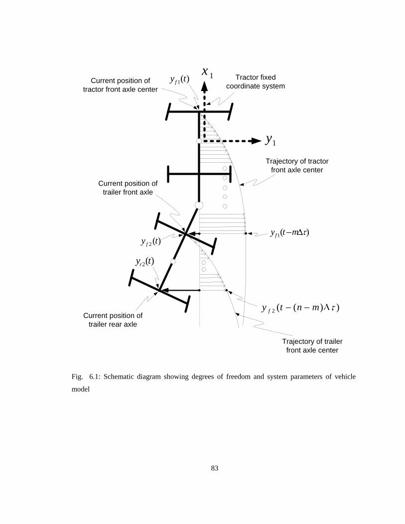
83

Current position of

tractor front axle center

Current position of

trailer front axle

Current position of

trailer rear axle

Trajectory of trailer

front axle center

Trajectory of tractor

front axle center

)(1 mty f

)(2 ty f

))((2 mnty f

)(2 tyr

Tractor fixed

coordinate system

1y

1x)(1 ty f


model

84

6.3.2 Design Criteria

To implement the above strategy, the controller is designed based on the linear quadratic

regulator (LQR) theory in the continuous time domain. The mathematical expression of

cost function of the LQR controller is devised as follows

(6.1)

The significance of each term of the above cost function can be described with the aid of

Fig. 6.1. In the first term represents the lateral position deviation

of the trajectory of the tractor front axle center trajectory with respect to that of the trailer

front axle center. The weighting factor imposes penalty upon the magnitude and

direction of this deviation. This penalty implies that the ATS system should locate the

current position of the trailer front axle center on the trajectory of tractor front axle

center denoted as . Note that all the deviations are expressed in the body-

fixed coordinate system of tractor.

Similarly the weighting factor punishes the magnitude and direction of the

expression as shown in the second term of cost function of

equation (6.2). The physical meaning of this expression is that at any instant , the current

position of the trailer rear axle center should be on the trajectory of the trailer front

axle center . Note that the time delay represents the time

85

required for the trailer rear axle center to reach the current location of trailer front axle

center.

In equation (6.2), is the weighting factor that imposes penalties upon the

magnitude and duration of the lateral position deviation of the trailer rear axle center

from the longitudinal axes of the tractor and trailer. The goal for introducing this term is

to prevent the dangerous jack-knifing motion mode during lane change and tight curved

path negation maneuvers. Note that the fourth and fifth terms on the right side of

equation (6.2) represent the energy consumption of the active trailer steering system.

Introducing these two terms will minimize the required energy consumption.

6.3.3 CLPDP Controller Design

Based on the design criteria in terms of the cost function expressed in equation (6.2), the

3-DOF vehicle model described in Subsection 3.2.2 cannot be incorporated directly in the

design of the CLPDP controller. The vehicle model should be modified to include the

required state variables: 1) lateral displacement of the tractor front axle center ; 2)

lateral displacement of the trailer front axle center ; and 3) lateral displacement of the

trailer rear axle center . Moreover, the modified vehicle model should consider the

time delays and for the state variables and , respectively. The

differential equations associated with the newly introduced state variables are constructed

as follows,

(6.2a)

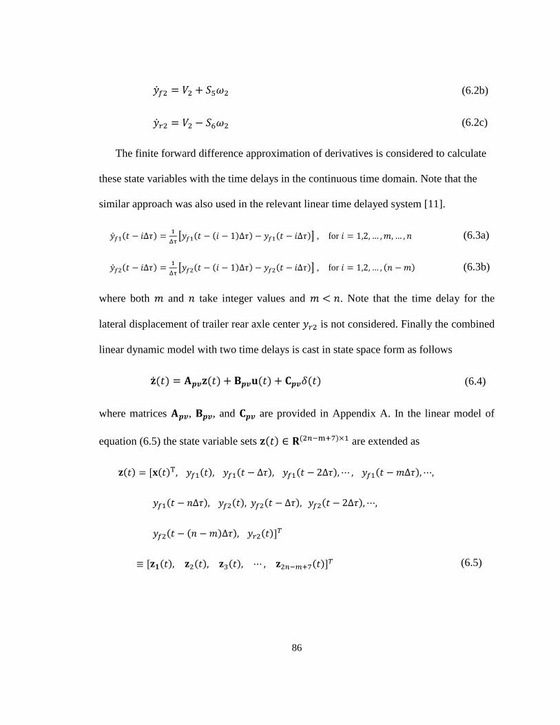
86

(6.2b)

(6.2c)

The finite forward difference approximation of derivatives is considered to calculate

these state variables with the time delays in the continuous time domain. Note that the

similar approach was also used in the relevant linear time delayed system [11].

, for (6.3a)

, for (6.3b)

where both and take integer values and . Note that the time delay for the

lateral displacement of trailer rear axle center is not considered. Finally the combined

linear dynamic model with two time delays is cast in state space form as follows

(6.4)

where matrices , , and are provided in Appendix A. In the linear model of

equation (6.5) the state variable sets are extended as

(6.5)

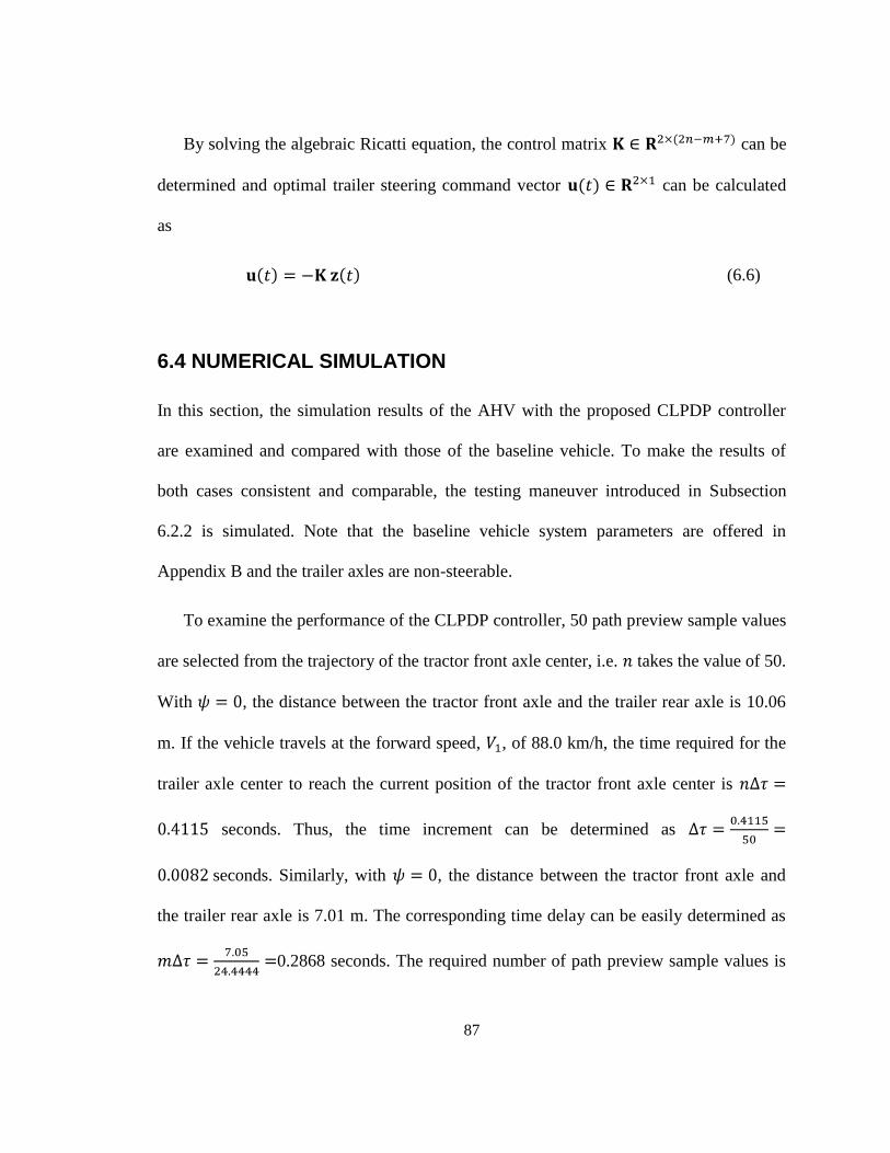
87

By solving the algebraic Ricatti equation, the control matrix can be

determined and optimal trailer steering command vector can be calculated

as

(6.6)

6.4 NUMERICAL SIMULATION

In this section, the simulation results of the AHV with the proposed CLPDP controller

are examined and compared with those of the baseline vehicle. To make the results of

both cases consistent and comparable, the testing maneuver introduced in Subsection

6.2.2 is simulated. Note that the baseline vehicle system parameters are offered in

Appendix B and the trailer axles are non-steerable.

To examine the performance of the CLPDP controller, 50 path preview sample values

are selected from the trajectory of the tractor front axle center, i.e. takes the value of 50.

With , the distance between the tractor front axle and the trailer rear axle is 10.06

m. If the vehicle travels at the forward speed, , of 88.0 km/h, the time required for the

trailer axle center to reach the current position of the tractor front axle center is

seconds. Thus, the time increment can be determined as

seconds. Similarly, with , the distance between the tractor front axle and

the trailer rear axle is 7.01 m. The corresponding time delay can be easily determined as

0.2868 seconds. The required number of path preview sample values is

88

calculated through . Note that if takes the nearest integer

value, this may degrade vehicle performance. To minimize this negative impact, the total

number of sample values n should take a large integer value. The weighting factor vector

is assigned the value of [0.5672, 1.8437, 3.3753, 0.4867,

0.4702] using the weighting factor determination procedure reported in [13, 4].

The general goal of the CLPDP controller is to make the trailer to follow the tractor

with adequate fidelity in a safe and stable manner. From stability point of view, the lower

the RWA ratio, the better the stability. However, if the RWA ratio takes very small value,

the trailer will not follow the path of the tractor. It is recommended that the RWA ratio

take the value of 1.0 [1]. This RWA ratio may make the lateral accelerations for both the

tractor and trailer comparable as well as comparable trajectories for both units.

Table 6.1: Selected simulation results for the baseline vehicle and the one with the CLPDP

controller

Baseline vehicle Vehicle with CLPDP

controller

RWA Ratio 1.2024 0.8980

Transient PFOT (m) 0.0631 0.0480

Steering sine-wave amplitude A (radian) 0.0044 0.0508

Table 6.1 offers the selected simulation results for the vehicle with the CLPDP

controller and those for the baseline vehicle. The RWA ratio of the vehicle with the

controller is 0.8980 and it is closer to the ideal value of 1.0 compared against the baseline

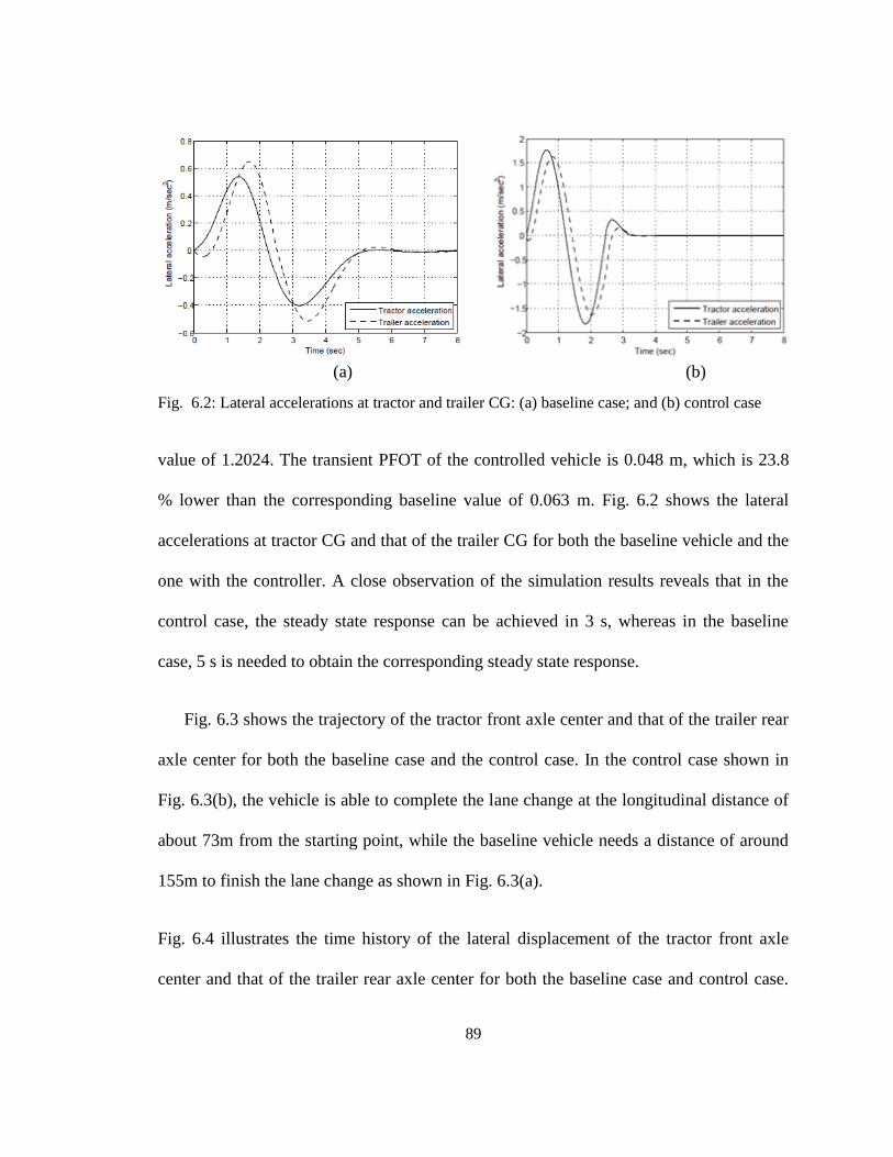
89

(a) (b)

Fig. 6.2: Lateral accelerations at tractor and trailer CG: (a) baseline case; and (b) control case

value of 1.2024. The transient PFOT of the controlled vehicle is 0.048 m, which is 23.8

% lower than the corresponding baseline value of 0.063 m. Fig. 6.2 shows the lateral

accelerations at tractor CG and that of the trailer CG for both the baseline vehicle and the

one with the controller. A close observation of the simulation results reveals that in the

control case, the steady state response can be achieved in 3 s, whereas in the baseline

case, 5 s is needed to obtain the corresponding steady state response.

Fig. 6.3 shows the trajectory of the tractor front axle center and that of the trailer rear

axle center for both the baseline case and the control case. In the control case shown in

Fig. 6.3(b), the vehicle is able to complete the lane change at the longitudinal distance of

about 73m from the starting point, while the baseline vehicle needs a distance of around

155m to finish the lane change as shown in Fig. 6.3(a).

Fig. 6.4 illustrates the time history of the lateral displacement of the tractor front axle

center and that of the trailer rear axle center for both the baseline case and control case.

90

In the control case, the tractor and trailer reach the lateral displacement of 1.46 m at 3.04

and 3.47 s, respectively, while in the baseline case, the tractor and trailer first achieve this

(a) (b)

Fig. 6.3: Trajectories of tractor and trailer front axle center in global coordinate system: (a)

baseline case; and (b) control case

Fig. 6.4: Time history of lateral displacement of tractor front axle center and that of trailer rear

axle center for baseline case and control case

lateral displacement at 6.30 s and 6.75 s, correspondingly. Thus, the vehicle with the

controller can complete the lane change much faster than the baseline vehicle. Note that

the vehicle with the CLPDP control achieves the above superior performance under the

91

condition of larger driver steering angle input than that used for the baseline vehicle as

shown in Table 6.1.

6.5 CONCLUSIONS

This chapter presents a compound lateral position deviation preview (CLPDP) control

scheme for active trailer steering (ATS) systems to improve high-speed stability of

articulated heavy vehicles (AHVs). The proposed CLPDP controller has been designed

using linear quadratic regulator (LQR) algorithm in the continuous time domain. To

examine the performance of the controller, it has been applied to the design of a

tractor/full-trailer combination with an ATS system. To perform numerical simulations, a

3 degree of freedom vehicle model is generated to represent the tractor/full-trailer system.

The resulting design based on the controller is compared with the baseline vehicle.

Numerical simulation results of a high-speed lane change maneuver show that the vehicle

with the controller is superior to the baseline vehicle in the performance measures of high-

speed lateral stability. In the case of control, the transient PFOT is reduced by 23.93%

compared against the baseline value. The vehicle with the controller can complete the lane

change much faster than the baseline vehicle, the former finishing this maneuver in about

3.47 seconds but the latter in 6.75 seconds. Moreover, the Rear-Ward Amplification ratio

for the baseline case is 1.2024, while the corresponding value for the control case is

0.8980. Thus, the latter is closer to the ideal value of 1.0.

The above simulation results indicate that the CLPDP controller can improve the

high-speed performance of the tractor/full-trailer combination. In the near future, the

92

effects of the controller on the low-speed performance of the vehicle system will be

examined and evaluated.

93

Chapter 7

CONCLUSIONS

7.1 INTRODUCTION

As discussed and identified in Chapter 1, the ultimate objective of this thesis is to develop

a novel method for the design method of articulated heavy vehicles (AHVs) with active

trailer steering (ATS) systems. The numerical simulation results reveal that the goal has

been successfully achieved. The feasibility and efficacy of the method has been

demonstrated by optimizing the high-speed stability and low-speed maneuverability of a

tractor/full-trailer combination. This design synthesis method and the numerous

conclusions drawn from the above numerical experiments are believed to be important

contributions to the design optimization of articulated heavy vehicles with active steering

systems.

In this chapter, the achievements of the research are addressed and the related areas

for future research are proposed.

7.2 PROPOSED SYNTHESIS METHOD

In the thesis, a single design loop (SDL) method has been compared with a two design

loop (TDL) method through the design synthesis of a tractor/full-trailer with an ATS

system. Compared with TDL method, the SDL approach searches solutions in a much

94

larger design space and consequently it provides a more comprehensive set of optimal

designs. This comprehensive set of optimal designs can be classified into three subsets

RWA (Rear-Ward Amplification) set for improving high-speed lateral stability

PFOT (Path-Following Off-Tracking) set for enhancing low-speed

maneuverability

Pareto set for optimal trade-off condition between the high-speed stability and

low-speed maneuverability

The simulation results illustrate that for the given design application, the SDL method

offers better trade-off design solutions than the TDL approach.

The SDL method can be used to automate the process of determining optimal values

of design for improving compatibility of the fundamental conflicting design criteria of

AHVs, i.e. low-speed maneuverability and high-speed stability. The SDL method has the

following distinguished features:

1. The optimal active design variables of ATS systems and optimal passive vehicle

system design variables are searched in a single design loop,

2. In the design process, to evaluate the vehicle performance measures a driver

model is developed and it „drive‟ the vehicle model based on the well-defined

testing specifications, and

95

3. The ATS controller designed from this method has two operational methods; one

for improving the lateral stability at high speeds, and the other for enhancing path-

following at low speeds.

The proposed SDL method may be used for identifying desired design variables and

predicting performance envelops in the early design stages of AHVs with ATS systems.

7.3 COMPOUND LATERAL POSITION DEVIATION PREVIEW

CONTROLLER

This thesis also proposed, developed and tested a compound lateral position deviation

preview (CLPDP) controller for ATS systems of AHVs to improve high-speed stability.

The proposed controller has the following features:

It is designed using linear quadratic regulator (LQR) algorithm in the continuous

time domain,

Time delay is taken into account to control the relevant trailer axle tires, and

The controller utilizes a compound set of preview information of the lateral

position deviation.

The numerical simulation results of a high-speed lane change maneuver show that the

vehicle with the controller is superior to the baseline vehicle in the performance measures

of high-speed lateral stability.

96

7.4 DIRECTIONS FOR FUTURE RESEARCH

To improve the proposed design synthesis method for AHVs with ATS system, the

following directions for future research are recommended.

1. Implementation in Parallel Computations Environment. The method is

suitable for applications using massively-parallel computers and the computation

time could be reduced approximately by a factor of the population size of the GA

[8].

2. Application to the Design Optimization of AHVs with Integrated Control

Systems. The anti-lock braking system, all tire steering system, and active

suspension system are based on three different directions of road vehicle

dynamics, i.e. longitudinal, lateral, and vertical respectively. The proposed

method is readily applicable to the design of AHVs with an integrated control

system where the three control systems can co-operate each other. Moreover, the

mechanical system and control system of AHV, with the method, can be

optimized simultaneously.

The limitation of the application of the proposed method is that the associated

computational burden is heavy. However, parallel processing, for which the method is

ideally suited, could be used for decreasing the total computer time required for the

optimization.

Although the method was originally intended for the design optimization of

articulated heavy vehicles (AHVs) with active trailer steering (ATS) system, this general

97

design method is also applicable to the design of other complex dynamic systems, e.g.

robots, and the other mechatronic systems, with minor modifications.

98

Bibliography

[1] Fancher, P. and Winkler, D. 2007. Directional performance issues in evaluation

and design of articulated heavy vehicles, Vehicle System Dynamics, 45(7-8), 607-

647,.

[2] Vlk, F. 1985. Handling Performance of Truck-Trailer Vehicles: A State-of-the-

Art Survey, Int. J. Of Vehicle Design 6(3), 323-361.

[3] Chen, B. and Peng, H. 1999. Rollover Warning For Articulated Vehicles Based

on A Time-To-Rollover Metric”, ASME International Mechanical Engineering

Conference and Exhibition, November.

[4] El-Gindy, M., Mrad, N. and Tong, X. 2001. Sensitivity of rearward amplification

control of a tractor/full trailer to tyre cornering stiffness variable, Proc. IMechE,

Part D: J. Automobile Engineering, 215, 579-588.

[5] National Highway Traffic Safety Administration: Traffic Safety Facts 1993 -

1998: A Compilation of Motor Vehicle Crash Data from the Fatality Analysis

Reporting System and the General Estimates System, 1994 - 1999.

[6] Gerum, E., Laszlo, P., Semsey, A., and Barta, G. 1998. Method for drive stability

enhancement of multi-unit vehicles. U.S. Patent 5 747 683, May 5.

[7] Anderson, R., Elkins, J. And Brickle, B. 2001. Rail Vehicle Dynamics for the

21th Century”, Proceedings of ICTAM‟2000, Chicago, USA.

[8] He, Y. 2003. Design of Rail Vehicles with Passive and Active Suspensions Using

Multidisciplinary Optimization, Multibody Dynamics, and Genetic Algorithms”,

PhD thesis, University of Waterloo, Waterloo, Ontario, Canada.

99

[9] He, Y. 2005. Khajepour, A., McPhee, John, and Wang, X., “Dynamic Modeling

and Stability Analysis of Articulated Frame Steer Vehicles. Int. J. Of Heavy

Vehicle Systems, 12(1), 28-59.

[10] Islam, M.M., and He, Y. 2008. Stability Optimization of Articulated Frame Steer

Vehicles”, 2nd

CIRP Conference on Assembly Technologies and Systems,

Toronto, Canada.

[11] Islam, M. and He, Y. 2009. Design synthesis of heavy articulated vehicles with

rearward amplification control, In Proceedings of the 22nd

Canadian Congress of

Applied Mechanics, Dalhousie University, Halifax, Canada, pp. 131-132.

[12] He, Y., Islam, M.M. and Webster, T.D. 2010. An integrated design method for

Articulated Heavy Vehicles with Active Trailer Steering Systems”, accepted by

SAE 2010 World Congress, SP-2261, SAE paper No. 2010-1-0092.

[13] Islam, M.M., He, Y., and Webster, T.D. 2010. Automated design synthesis of

articulated heavy vehicles with active trailer steering systems”, accepted by ASME

IDETC/CIE 2010, Paper No: DETC2010-28160.

[14] Wu, D.H. 2001. A Theoretical Study of the Yaw/Roll Motions of A Multiple

Steering Articulated Vehicle, Proceedings Institutions of Mech. Engg., Vol. 215,

Part D.

[15] Winkler, C.B., Blower, D., Ervin, R.D. and Chalasani, R.M. 2000. Rollover of

Heavy Commercial Vehicles”, SAE, Warrendale, PA, USA.

[16] Miege, A.J.P. 2003. Active Roll Control of an Experimental Articulated Vehicle.

Cambridge University Engineering Department, PhD Dissertation.

100

[17] Anon. 2002. Road Accidents in Great-Britain. Department of Transport, HMSO,

UK.

[18] Rakheja, S., Sankar, S. and Ranganthan, R. 1987. Roll plane analysis of

articulated tank vehicles during steady turning. Vehicle System Dynamics, 17(2),

pp. 81–104.

[19] Broge, J.L. 2000. Heavy duty truck safety systems. Automotive Engineering

International, pp. 101–105.

[20] Anon. 2001. Traffic Safety Facts 2000: A compilation of motor vehicle crash data

from the Fatality Analysis Reporting System and the General Estimates System.

Technical Report DOT HS 809 337, National Highway Traffic Safety

Administration, National Center for Statistics and Analysis, Washington DC,

USA.

[21] Erkert, T.W., Sessions, J., Layton,R.D. 1989. A Method for Determining off-

tracking of multiple unit vehicle combinations”, Int. J. Of Forest Engg., 1989.

[22] He, Y., Khajepour, A., McPhee, J. and Wang, X. 2005. Dynamic modelling and

stability analysis of articulated frame steer vehicles, Int. J. Heavy Vehicle

Systems, 12(1), 28-59.

[23] He, Y. and McPhee, J. 2005. A design method for mechatronic vehicles:

application of multidisciplinary optimization, multibody dynamics and genetic

algorithms”, Vehicle System Dynamics, 43(10), 697-733.

[24] Christensen, T.C., and Blythe, W. 2000. Offtracking: History, Analysis, and

Simulation, SAE 2000 World Congress, 2000-01-0465, Detroit, MI, USA, March.

101

[25] Palkovics, L. and Fries, A. 2001. Intelligent electronic systems in commercial

vehicles for enhanced traffic safety, Vehicle System Dynamics, 35(4-5), 227-289.

[26] Prem, H., Ramsay, E., Pont, J., McLean, J. and Woodrooffe, J. 2001.

Comparison of modelling systems for performance-based assessments of heavy

vehicles (Performance based standards – NRTC/Austroads project A3 and A4),

The National Road Transport Commission (NRTC), Working Paper, October.

[27] Winkler, C.B., Fancher, P.S., Bareket, Z., Bogard, S.E., Johnson, G., Karamihas,

S.M. and Mink, C.E. 1992. Heavy vehicle size and weight: test procedures for

minimum safety performance standards. Final technical report”, Transportation

Research Institute, Michigan University: Ann Arbor, 118 p. UMTRI-92-

13/DTNH-22-87-D-17174.

[28] Odhams, A., Roebuck, R., Cebon, D. and Winker, C. 2008. Dynamic safety of

active trailer steering systems, Proc. IMechE, Part K: J. Multi-body Dynamics,

222, 367-380.

[29] Rangavajhula, K. and Tsao, H-S. J. 2007. Active steering control of an articulated

system with a tractor and three full trailers for tractor-track following, Int. J.

Heavy Vehicle Systems, 14(3), 271-293.

[30] Rangavajhula, K. and Tsao, H-S. J. 2008. Command steering of trailers and

command-steering-based optimal control of an articulated system for tractor-track

following, Intn. Mech. Engrs., Vol.222, 2008. Proc. IMechE, Part D: J.

Automobile Engineering, 222, 935-954.

102

[31] Aurell, J. and Edlund, S. 1989. The Influence of Steered Axles on the Dynamic

Stability of Heavy Vehicles, SAE paper No. 892498.

[32] Jujnovich, B. and Cebon, D. 2002. Comparative performance of semi-trailer

steering systems. In proceedings of the 7th

International Symposium on Heavy

Vehicle Weights and Dimensions, Delft, pp. 195-214.

[33] Wu, D-H. and Lin, J. H. 2003. Analysis of dynamic lateral response for a multi-

axle-steering tractor and tractor and trailer”, Int. J. of Heavy Vehicle Systems,

10(4), 281-294.

[34] Ellis, J. R. 1969. Vehicle Dynamics, Business Books Limited, London.

[35] Society of Automotive Engineers, A test for evaluating the rearward amplification

of multi-articulated vehicles, SAE Recommended Practice J2179, SAE,

Warrendale, USA, 1994.

[36] Rules for the Assessment of Potential Performance-Based Standards. Discussion

Paper. National Transport Commission (NTC), Australia, June 2005.

[37] Bryson, A. and Ho, Y. 1975. Applied optimal control, optimization, estimation

and control, Wiley, New York.

[38] Karnopp, D. 1990. Design principles for vibration controls systems using semi-

active dampers, Journal of Dynamics Systems Measurement Control, 112, 448-

455.

[39] Goldberg, D. 1989. Genetic algorithms in search, optimization, and machine

learning, Addison-Wesley, Reading, MA.

103

[40] Thompson, A.G. 1976. An Active Suspension with Optimal Linear State

Feedback, Vehicle System Dynamics, 5, 187-203.

[41] Palkovics, L., Semsey, A. and Gerum, E. 1998. Roll-Over Prevention System for

Commercial Vehicles – Additional Sensorless Function of the Electronic Brake

System. AVEC‟98, Paper No. 9837409.

[42] "Truck and Bus Crash Factbook. 1995. University of Michigan Transportation

Research Institute, Center for National Truck Statistics, UMTRI-97-30.

[43] Sankar, S., Rakhija, S. and Piche, A. 1991.Directional dynamics of a tractor –

semi-trailer with self and force steering axles, SAE Transactions, SAE 912686.

[44] Lewis, A.S. and El-Gindy, M. 2003. Sliding mode control for rollover prevention

of heavy vehicles based on lateral acceleration”, Heavy Vehicle Systems, A

Special Issue of the Int. J. of Vehicle Design, Vol. 10, Nos. 1/2, pp. 9–34.

[45] Harwood, D.W., Potts, I.B., Torbic, D.J., and Glauz, W.D. 2003. Highway/Heavy

Vehicle Interaction”, Commercial Truck and Bus Safety Synthesis Program

CTBSSP-SYN-3, ISBN-0-309-08756-2. Washington, DC: Transportation

Research Board.

[46] Fenwick SV, Harris JapC. 1999. The application of Pareto frontier methods in the

multidisciplinary wing design of a generic modern military delta aircraft. In

proceedings of NATO RTO AVT symposium, Ottawa, October.

[47] Abbass, H A, Sarker, R, and Newton C. 2001. PDE: A Paretofrontier differential

evolution approach for multi-objective optimization problems”, Proc. of IEEE

Congress on Evolutionary Computation. pp 971-978.

104

[48] J. Cao, J. Lin. 2008. A Study on Formulation of Objective Functions for

Determining Material Models”, Int. J. Mech. Sci., 50: 193-204, 2008.

[49] Rangavajhula, K. and Tsao, H.-S. J. Effect of multi-axle steering on off-tracking

and dynamic lateral response of articulated tractor–trailer Combinations. Int. J.

Heavy Veh. Systems, 14(4), 376–401.

[50] Tsao, H.-S. J., Dessouky, Y., Rangavajhula, K., Zeta, J. B., and Zhou, L. 2006.

Automatic steering for conventional truck trailers: development and assessment of

operating concepts for improving safety, productivity and pavement durability –

final report, PATH Research Report UCB-ITS-PRR-2006- 8, Institute of

Transportation Studies, University of California, Berkeley.

[51] Road Vehicles–Heavy Commercial Vehicle Combinations and Articulated Buses-

Lateral Stability Test Methods (2nd edn) (International Organization for

Standardization: Geneva, Switzerland), 12 p. ISO 14790:2000(E).

[52] A test for evaluating the rearward amplification of multi-articulated vehicles.

Standard J2179, Society of Automotive Engineers, September 1993.

[53] MacAdam, C.C. 1988. Development of driver/vehicle steering interaction models

for dynamic analysis,” Tech. Rep. U.S. Army Tank–Automotive Command, Univ.

Michigan Transportation Res. Inst., Report UMTRI-88-53.

[54] Prem, H., Ramsay, E.D., De Pont, J., McLean, J.R. and Woodrooffe, J.H. 2001b.

Comparison of Modelling Systems for Performance-Based Assessments of Heavy

Vehicles, Working Paper prepared for the National Road Transport Commission

105

by RTDynamics, TERNZ Ltd, J.R. McLean and Woodrooffe & Associates Inc,

Melbourne, Vic. October.

[55] DiCristoforo, Rob, Blanksby, Chris, and Germanchev, 2006. Anthony.

Performance-Based Certification of an Innovative Truck-Trailer Configuration

for the Safer and More Efficient Distribution of Liquid Fuel in Australia. ARRB

Group Ltd., written for the Transportation Research Board Annual Meeting,

Washington, D.C.

[56] Cohen, H. 2009. Wisconsin Truck Size and Weight Study, Wisconsin Department

of Transportation.

[57] Tanaka K, Kosaki T. 1997 Design of a stable fuzzy controller for an articulated

vehicle”, IEEE Trans Syst Man Cybern B Cybern,27(3):552-8.

[58] Winkler, C. B., P. Fancher, P. S., Carsten, O., Mathew, A., Dill, P. 1986.

Improving The Dynamic Performance Of Multitrailer Vehicles: A Study Of

Innovative Dollies”, Transportation Research Institute (UMTRI), University of

Michigan, Ann Arbor.

[59] Fancher, P., Winkler, C., Ervin, R. and Zhang, H. 1997. Using Braking to Control

the Lateral Motions of Full Trailers”, The Dynamics of Vehicle on Roads and on

Tracks. Proceedings of the 15th IAVSD Symposium, Budapest, Hungary, August

25-29, pp. 462-478.

[60] Antoniou, A ., and Lu, W-S. 2007. Practical optimization: algorithms and

engineering applications”, Springer, New York.

106

[61] Fakhreddine, O.K., and Clarence, D.S. 2004. Soft Computing and Intelligent

Systems Design”, Pearson, Harlow (UK).

[62] Holland, J. 1975. Adaptation in Natural and Artificial Systems”, University of

Michigan Press, Ann Arbor.

[63] Kalman, R.E. 1960. Contribution to the Theory of Optimal Control”, Bol. Soc.

Matem. Maxico, 102-119.

[64] Kalman, R.E. 1964. When is a Linear Control System Optimal?”, ASME

transactions Series D (Journal of Basic Engineering), 51-60.

[65] Dutta, A., Bhattacharya, S., Keel, L.H. 2009. Linear Control Theory: Structure,

Robustness and Optimization”, CRC press, Florida.

[66] Janson, B.N., Awad, W., Robles, J., Kononov, J. and Pinkerton, B. 1998. Truck

accidents at freeway ramps: data analysis and high-risk site identification”,

Journal of Transportation and Statistics, 75-92, January.

[67] Sharp, R. S. 2005. Driver steering control and a new perspective on car handling

qualities”, Proc. IMechE, Part C: J. Mechanical Engineerig Science, vol. 219, pp.

1041-1051.

[68] Sun, J. Q., and Song, B. 2009. Control Studies of Time-Delayed Dynamical

Systems with the Method of Continuous Time Approximation", Communications

in Nonlinear Science and Numerical Simulation, vol. 14, pp. 3933-3944.

[69] Cheng, C., and Cebon, D. 2008. Improving roll stability of articulated heavy

vehicles using active semi-trailer steering”, Vehicle System Dynamics, vol. 46,

pages 373-388.

107

APPENDEX

APPENDIX A: VEHICLE MODEL SYSTEM MATRICES

where matrices , , , , , , , , (and also for Model-1) are defined

as follows

108

The matrices M, N, P, , and are given below

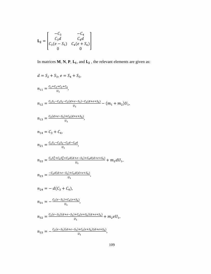
109

In matrices M, N, P, , and , the relevant elements are given as:

, ,

,

,

,

,

,

,

,

,

,

,

,

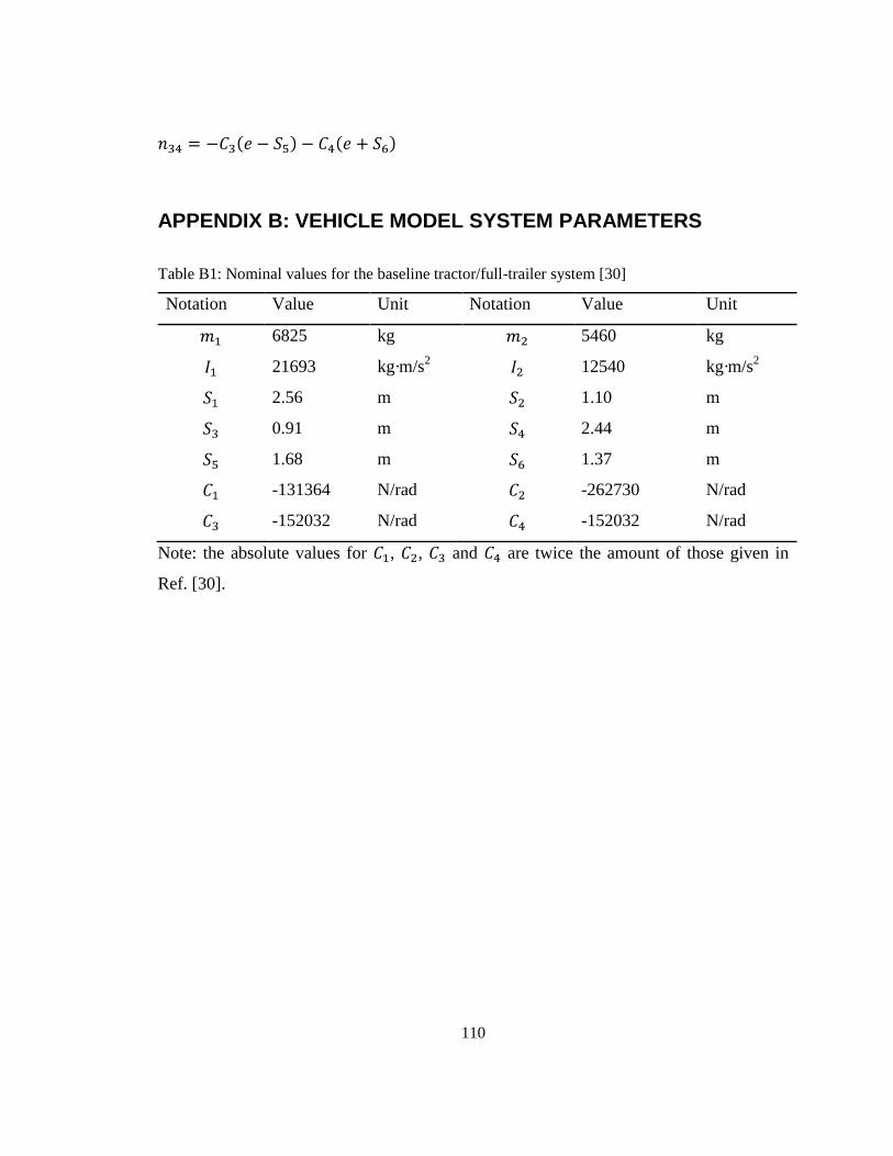
110

APPENDIX B: VEHICLE MODEL SYSTEM PARAMETERS

Table B1: Nominal values for the baseline tractor/full-trailer system [30]

Notation Value Unit Notation Value Unit

6825 kg 5460 kg

21693 kg·m/s2

12540 kg·m/s2

2.56 m 1.10 m

0.91 m 2.44 m

1.68 m 1.37 m

-131364 N/rad -262730 N/rad

-152032 N/rad -152032 N/rad

Note: the absolute values for , , and are twice the amount of those given in

Ref. [30].

Documents

Design Synthesis of Articulated Heavy Vehicles With Active Trailer Steering Systems