Embed Size (px)
Citation preview

Design of Earthquake Resistant Bridges Using Rocking Columns
by
Clément Benjamin Barthès
A dissertation submitted in partial satisfaction of therequirements for the degree of
Doctor of Philosophy
in
Engineering- Civil and Environmental Engineering
in the
Graduate Division
of the
University of California, Berkeley
Committee in charge:
Professor Bozidar Stojadinovic, ChairProfessor Filip C. FilippouProfessor John A. Strain
Spring 2012

Design of Earthquake Resistant Bridges Using Rocking Columns
Copyright 2012by
Clément Benjamin Barthès

Abstract
Design of Earthquake Resistant Bridges Using Rocking Columns
by
Clément Benjamin Barthès
Doctor of Philosophy in Engineering- Civil and Environmental Engineering
University of California, Berkeley
Professor Bozidar Stojadinovic, Chair
The California Department of Transportation (CalTrans) is urging researchers and con-tractors to develop the next generation highway bridge design. New design solutions shouldfavor the use of modular construction techniques over conventional cast-in-place reinforcedconcrete in order to reduce the cost of the projects and the amount of constructions on site.Earthquake resistant bridges are designed such that the columns are monolithically con-nected to the girder and the foundations. Hence, despite the great improvements recentlymade in modular bridge construction, a large amount of concrete is still cast in place toproperly splice the reinforcements between the segments.
Instead of designing earthquake resistant bridges with monolithic joints, it is proposedto use discontinuous connections in this thesis. The segments may rock at their interfaceduring a severe earthquake and, if rocking rotation is too large, the structure may collapse.However, if a bridge is allowed to rock moderately, it may modify the earthquake responseand drastically reduce the resisting forces within the structure.
The research presented in this dissertation focuses on the modeling of rocking connec-tions. First, the behavior of rocking rigid blocks under earthquake excitation is studied. Itis proposed to restrain the rigid blocks with an unbonded post-tensioning cable in order toallow rocking but prevent overturning. The findings made on rigid blocks, however, cannotbe applied to deformable structures because of the limitations of the model. Therefore, acompletely different approach is proposed. Instead of modeling the behavior of an entireblock, it is proposed to model only the rocking surface. A zero-length finite element is de-veloped, allowing to represent the in-plane rocking rotation between two frame elements. Itallows to investigate the behavior of a deformable column rocking freely on its base as well asthe stability of a rocking column restrained with a cable and subjected to a large earthquakeexcitation. The consequences of a post-tensioning cable failure and yielding of the columnare also investigated. It is proposed to add a dissipative fuse between the base of the column
1
and its footing in order to enhance the stability of the structure. Finally, the behavior ofa conventional monolithic bridge is compared with a bridge allowed to rock at the columnsjoints.
The results obtained with the rigid block model show that, when columns are allowed torock under earthquake excitation, it is possible to adjust the response and preserve stabilitywith a Post-Tensioning (PT) cable. The implementation of the zero-length rocking elementpermits to study the behavior of deformable structures that are allowed to rock. At first, thiselement is used in combination with a very stiff elastic element and the results are consistentwith the response of a rigid block. This element shows that the free rocking response ofan elastic column may stop rocking and start to oscillate in flexure. The dissipative fuse incombination with a long unbonded PT cable proves to be effective. However, it is shownthat, if the dissipative fuse is too large, it may prevent the column from returning to itsinitial position. At last, it is shown that a bridge structure allowed to rock and restrainedwith cables can sustain a large earthquake. The resisting moments within the columns aregreatly reduced when compared with a conventional bridge while the drift ratio remainsmoderate.
Several subjects are left for further research. First, the zero-length rocking element rep-resents rocking only in the plane of the frame. The development of a 3D rocking elementis challenging because the column may rock and roll and may also twist around one corner.The design of the rocking surface is not investigated; a bridge prototype should be designedand tested experimentally to validate the feasibility of the solution proposed in this study.
2
Contents1 Introduction 1
2 Modular Bridge Construction 42.1 Introduction . . . . . . . . . . . . . . . . . . . . . . . . . . . . . . . . . . . . 42.2 Existing Precast Elements Connections . . . . . . . . . . . . . . . . . . . . . 5
2.2.1 Grouted Pockets . . . . . . . . . . . . . . . . . . . . . . . . . . . . . 82.2.2 Self-Compacting Concrete . . . . . . . . . . . . . . . . . . . . . . . . 10
2.3 Bridge Columns With Unbonded Segments . . . . . . . . . . . . . . . . . . . 122.4 Repairability of Modular Bridges . . . . . . . . . . . . . . . . . . . . . . . . 15
3 Rigid Blocks Subjected to Rocking 173.1 Single Block Rocking Behavior . . . . . . . . . . . . . . . . . . . . . . . . . . 17
3.1.1 Assumptions . . . . . . . . . . . . . . . . . . . . . . . . . . . . . . . . 173.1.2 SDOF Vibration Analogy . . . . . . . . . . . . . . . . . . . . . . . . 223.1.3 Rocking termination . . . . . . . . . . . . . . . . . . . . . . . . . . . 23
3.2 3D Rocking Block . . . . . . . . . . . . . . . . . . . . . . . . . . . . . . . . . 263.3 Two-block Rocking Assemblies . . . . . . . . . . . . . . . . . . . . . . . . . . 293.4 Single Rocking Block Restrained With a Cable . . . . . . . . . . . . . . . . . 32
3.4.1 Implementation of the PT-RB Model . . . . . . . . . . . . . . . . . . 363.4.2 Free Vibration Response . . . . . . . . . . . . . . . . . . . . . . . . . 383.4.3 Response to a Ground Acceleration Pulse . . . . . . . . . . . . . . . . 38
3.5 Rocking Spectra . . . . . . . . . . . . . . . . . . . . . . . . . . . . . . . . . . 403.6 Design Strategy Using a Rocking Base . . . . . . . . . . . . . . . . . . . . . 423.7 Conclusion . . . . . . . . . . . . . . . . . . . . . . . . . . . . . . . . . . . . . 46
4 Rocking Element 484.1 Introduction . . . . . . . . . . . . . . . . . . . . . . . . . . . . . . . . . . . . 484.2 Description of the Element . . . . . . . . . . . . . . . . . . . . . . . . . . . . 494.3 Initiation of Rocking . . . . . . . . . . . . . . . . . . . . . . . . . . . . . . . 514.4 Implementation of the Constraints . . . . . . . . . . . . . . . . . . . . . . . . 534.5 Integration Scheme . . . . . . . . . . . . . . . . . . . . . . . . . . . . . . . . 584.6 Comparison with Rigid Block Solutions . . . . . . . . . . . . . . . . . . . . . 634.7 Rocking Termination . . . . . . . . . . . . . . . . . . . . . . . . . . . . . . . 654.8 Behavior of a Two-block Assembly . . . . . . . . . . . . . . . . . . . . . . . 674.9 Conclusion . . . . . . . . . . . . . . . . . . . . . . . . . . . . . . . . . . . . . 69
i

5 Rocking Analysis of Elastic Columns 705.1 Introduction . . . . . . . . . . . . . . . . . . . . . . . . . . . . . . . . . . . . 705.2 Rocking-Bending Interaction . . . . . . . . . . . . . . . . . . . . . . . . . . . 715.3 Damping . . . . . . . . . . . . . . . . . . . . . . . . . . . . . . . . . . . . . . 765.4 The effect of elastic deformations on rocking behavior . . . . . . . . . . . . . 815.5 Conclusion . . . . . . . . . . . . . . . . . . . . . . . . . . . . . . . . . . . . . 88
6 Behavior of Bridge Columns Allowed to Rock 896.1 Introduction . . . . . . . . . . . . . . . . . . . . . . . . . . . . . . . . . . . . 896.2 Yielding and Failure of the Restraining Cable . . . . . . . . . . . . . . . . . 926.3 Elastic-Perfectly Plastic Column . . . . . . . . . . . . . . . . . . . . . . . . . 996.4 Rocking Column with a PT Cable and a Dissipative Fuse . . . . . . . . . . . 1026.5 Conclusion . . . . . . . . . . . . . . . . . . . . . . . . . . . . . . . . . . . . . 113
7 Behavior of Bridges with Rocking Columns 1157.1 Introduction . . . . . . . . . . . . . . . . . . . . . . . . . . . . . . . . . . . . 1157.2 Single Column Bridge Results . . . . . . . . . . . . . . . . . . . . . . . . . . 1257.3 Two-Columns Bridge . . . . . . . . . . . . . . . . . . . . . . . . . . . . . . . 1327.4 Conclusion . . . . . . . . . . . . . . . . . . . . . . . . . . . . . . . . . . . . . 139
8 Summary and Conclusions 1408.1 Summary . . . . . . . . . . . . . . . . . . . . . . . . . . . . . . . . . . . . . 1408.2 Conclusions . . . . . . . . . . . . . . . . . . . . . . . . . . . . . . . . . . . . 1418.3 Recommendations for further research . . . . . . . . . . . . . . . . . . . . . 142
Bibliography 146
ii

List of Figures1 Typical multi-span California standard ordinary bridge . . . . . . . . . . . . 22 Monolithic design of a standard ordinary bridge . . . . . . . . . . . . . . . . 33 Reduced Moment at the Base of the Column . . . . . . . . . . . . . . . . . . 54 Precast Bent-Cap Installed on Site (Texas DOT) . . . . . . . . . . . . . . . 65 SPER System for Solid Section Columns [29] . . . . . . . . . . . . . . . . . . 66 SPER System for Hollow Section Columns [29] . . . . . . . . . . . . . . . . . 77 Grouted pocket connections between a precast column and a precast bent-cap 88 Trestle Type Prefabricated Concrete Columns [36] . . . . . . . . . . . . . . . 99 Self-Compacting Concrete being cast . . . . . . . . . . . . . . . . . . . . . . 1010 Congested Reinforcements . . . . . . . . . . . . . . . . . . . . . . . . . . . . 1111 Monolithic Bridge Substructure Assembly Subjected to Earthquake Motion . 1212 Unbonded Segmented Bridge Substructure Subjected to Earthquake Motion 1313 Cylinder Rocking . . . . . . . . . . . . . . . . . . . . . . . . . . . . . . . . . 1314 Bolted Longitudinal Reinforcements [4] . . . . . . . . . . . . . . . . . . . . . 1615 Description of the Rocking Block . . . . . . . . . . . . . . . . . . . . . . . . 1816 Moment vs. rotation of a RB . . . . . . . . . . . . . . . . . . . . . . . . . . 1917 Response of RBs to a Half-Cosine Ground Acceleration . . . . . . . . . . . . 2118 Rolling of a Cylinder on Its Edge (From [33]) . . . . . . . . . . . . . . . . . . 2619 Tombstone Rotated After Sanriku-Haruka-Oki Earthquake (1994) . . . . . . 2720 Rotation of a Rigid Block Subjected to a Skewed Earthquake Excitation . . 2821 2 Rigid Blocks Assembly (from [28]) . . . . . . . . . . . . . . . . . . . . . . . 2922 Rocking Modes for 2 Blocks Assemblies (from [28]) . . . . . . . . . . . . . . 3023 Free Rocking Response of a Two Rigid Blocks Assembly (from [28]) . . . . . 3124 Rocking Block with PT Cables . . . . . . . . . . . . . . . . . . . . . . . . . 3225 Strain in the Post-Tensioning Cable for θ = α . . . . . . . . . . . . . . . . . 3326 Restoring Moment Versus Rotation for α = 10◦ . . . . . . . . . . . . . . . . 3527 Continuous Functions f+ and f− Used By the ODE Solver . . . . . . . . . . 3728 Free Vibration Response With an Initial Rotation . . . . . . . . . . . . . . . 3829 Response of an Unprestressed RB to a Half-Cosine Pulse . . . . . . . . . . . 3930 Response of PT-RBs to a Half-Cosine Pulse . . . . . . . . . . . . . . . . . . 3931 Rocking Spectra of PT-RBs, Subjected to Kobe Earthquake . . . . . . . . . 4132 Typical Section of a Multi-Span Bridge . . . . . . . . . . . . . . . . . . . . . 4333 Bridge Column subjected to Tabas EQ . . . . . . . . . . . . . . . . . . . . . 4434 PT-RB with a partially bonded cable . . . . . . . . . . . . . . . . . . . . . . 4535 Bridge column subjected to Tabas EQ . . . . . . . . . . . . . . . . . . . . . 4536 Description of the Rocking Element . . . . . . . . . . . . . . . . . . . . . . . 49
iii

37 Kinematics of the Rocking Element . . . . . . . . . . . . . . . . . . . . . . . 5038 Augmented Lagrangian Method . . . . . . . . . . . . . . . . . . . . . . . . . 5439 Vertical Constraint of the Rocking Element Versus Rotation . . . . . . . . . 5540 Vertical Constraint of the Rocking Element With a Polynomial Interpolation 5641 Column With a Rocking Base . . . . . . . . . . . . . . . . . . . . . . . . . . 5742 Rocking Column Rotation and Angular Velocity . . . . . . . . . . . . . . . . 5743 Structures of the Integration Schemes . . . . . . . . . . . . . . . . . . . . . . 5844 Rocking Element Response to a Free Oscillation . . . . . . . . . . . . . . . . 6045 Spectral Radius of the HHT Integration Method . . . . . . . . . . . . . . . . 6146 Summary of the HHT Algorithm Implementation . . . . . . . . . . . . . . . 6247 Free Rocking Response With a Rocking Element . . . . . . . . . . . . . . . . 6448 Free Rocking Response, Then Subjected to a Large Ground Acceleration . . 6649 Free Rocking Response of a Two Rigid Blocks Assembly . . . . . . . . . . . 6750 Common Model Configuration for a Rocking Frame . . . . . . . . . . . . . . 7051 Elastic Column With a Lumped Mass and a Rocking Base . . . . . . . . . . 7152 Unscaled Pseudo-Acceleration Response Specrum . . . . . . . . . . . . . . . 7253 Acceleration Response of the structure subjected to Kobe (1995) . . . . . . . 7354 Clamped Elastic Column and Rocking Rigid Column . . . . . . . . . . . . . 7455 Base Rotations of a Rigid Column and an Elastic Column . . . . . . . . . . 7556 Free Rocking With Constant Damping Matrices . . . . . . . . . . . . . . . . 7757 Free Rocking With an Updated Damping Matrix . . . . . . . . . . . . . . . 7858 Rocking Rotation of a Cable Restrained Cantilever Column - Kobe EQ (1995) 7959 Free Rocking of a Column for Different Young’s Moduli . . . . . . . . . . . . 8260 Elastic Rocking Beam Es . . . . . . . . . . . . . . . . . . . . . . . . . . . . . 8361 Elastic Rocking Beam 10Es . . . . . . . . . . . . . . . . . . . . . . . . . . . 8462 Simplified Model of an Elastic Rocking Beam . . . . . . . . . . . . . . . . . 8563 Cantilever Column with a Short Restraining Cable . . . . . . . . . . . . . . 9064 Static Restoring Moment versus θ for a Column assumed to be rigid . . . . . 9365 Drift Ratio with Brittle Cable Failure . . . . . . . . . . . . . . . . . . . . . . 9466 Resisting Moment with Brittle Cable Failure . . . . . . . . . . . . . . . . . . 9567 Drift Ratio with Plastic Tie-rod . . . . . . . . . . . . . . . . . . . . . . . . . 9768 Resisting Moment with Plastic Tie-rod . . . . . . . . . . . . . . . . . . . . . 9869 Elastic Column With a Lumped Mass, a Plastic Hinge and a Rocking Base . 9970 Drift Ratio for an Elastic-Plastic Column . . . . . . . . . . . . . . . . . . . . 10071 Resisting Moment for an Elastic-Plastic Column . . . . . . . . . . . . . . . . 10172 Column with an Unbonded Restraining Cable and a Dissipative Fuse . . . . 10373 Rocking Rotation of a Column with Fuse . . . . . . . . . . . . . . . . . . . . 10574 Resisting Moment of a Column with Fuse . . . . . . . . . . . . . . . . . . . . 106
iv

75 The Fuse Prevents the Column to Return to its Initial Position . . . . . . . . 10876 Fuse Force and Plastic Strain . . . . . . . . . . . . . . . . . . . . . . . . . . 10977 Rocking Rotation of a Column with New Fuse . . . . . . . . . . . . . . . . . 11178 Cable Stress for a Column With Fuse . . . . . . . . . . . . . . . . . . . . . . 11279 Single Column Bridge Configuration . . . . . . . . . . . . . . . . . . . . . . 11680 Two-Columns Bridge Model . . . . . . . . . . . . . . . . . . . . . . . . . . . 11781 Drawing Outline of the Column Connections . . . . . . . . . . . . . . . . . . 11982 Force vs. Strain and Moment vs. Curvature for the Bridge Column . . . . . 12383 Structure Drift Ratio of the Single Column Bridge . . . . . . . . . . . . . . . 12584 Moment-Curvature at the Column Joints . . . . . . . . . . . . . . . . . . . . 12685 Resisting Moments at Column Joints of the Single Column Bridge . . . . . . 12786 Rocking Rotations at Column Joints of the Single Column Bridge . . . . . . 12887 Fuse’s Stress and Plastic Strain of the Single Column Bridge - Kobe (1995) . 12988 Restraining Cable Stress of the Single Column Bridge . . . . . . . . . . . . . 13089 Shear Demand on the Footing of the Single Column Bridge - Kobe (1995) . . 13190 Structure Drift Ratio of the Two-Columns Bridge . . . . . . . . . . . . . . . 13391 Moment-Curvature at the Column Joints - Non Rocking . . . . . . . . . . . 13492 Resisting Moments at Column Joints of the Two-Columns Bridge . . . . . . 13593 Rocking Rotations at Column Joints of the Two-Columns Bridge . . . . . . . 13694 Fuse’s Stress and Plastic Strain of the Two-Columns Bridge - Kobe (1995) . 13795 Shear Demand on the Footings of the Two-Columns Bridge - Kobe (1995) . . 138
v

List of Tables1 Column Properties . . . . . . . . . . . . . . . . . . . . . . . . . . . . . . . . 632 Blocks Properties . . . . . . . . . . . . . . . . . . . . . . . . . . . . . . . . . 683 Model properties . . . . . . . . . . . . . . . . . . . . . . . . . . . . . . . . . 724 Comparison of the rocking-elastic transition results with the simplified model 875 Model properties of the Rocking Column With a Short PT Cable . . . . . . 896 Model Properties of the Rocking Column With Fuse and PT Cable . . . . . 1047 Model Properties of the Second Dissipative Fuse . . . . . . . . . . . . . . . . 1108 Bridges Dimensions . . . . . . . . . . . . . . . . . . . . . . . . . . . . . . . . 1189 Bridge properties . . . . . . . . . . . . . . . . . . . . . . . . . . . . . . . . . 12010 Column Cross-Section properties . . . . . . . . . . . . . . . . . . . . . . . . 122
vi

AcknowledgmentsFirst and foremost, I would like to thank my advisor Professor Bozidar Stojadinovic for allhis help. He always encouraged me to pursue the research field that I was most interested in,yet he always directed me in the right way. Thank you very much for your time and effortspent on my PhD.
I would also like to thank Professor Filippou for his help on the development of myrocking element in FedeasLab as well as Professor Govindjee for sharing his knowledge withme on impact mechanics.
I am very grateful to Professor Ibrahimbegovic from my French University the EcoleNormale Supérieure of Cachan. His support allowed me to join the PhD program here atUC Berkeley.
I would also like to thank Professor Mosalam, who offered me an internship while I wasa master student. He introduced me to the field of experimental research and offered me awonderful experience that thrived me to pursue in this domain.
To my friend Dr. Véronique Le Corvec, I am very thankful for your help and for yoursupport. I have learned a lot from our countless discussions on our respective research.
I am very grateful to my parents Jean-Paul and Franoise as well as my sister Julie andmy brother Charles for always being very supportive, despite the distance.
Last and most of all, I would like to thank my wife Rika and our son Alexis, who wasborn a year ago in the course of my PhD. Their love and support are essential to me. Thisdissertation goes to them.
vii
1 INTRODUCTION
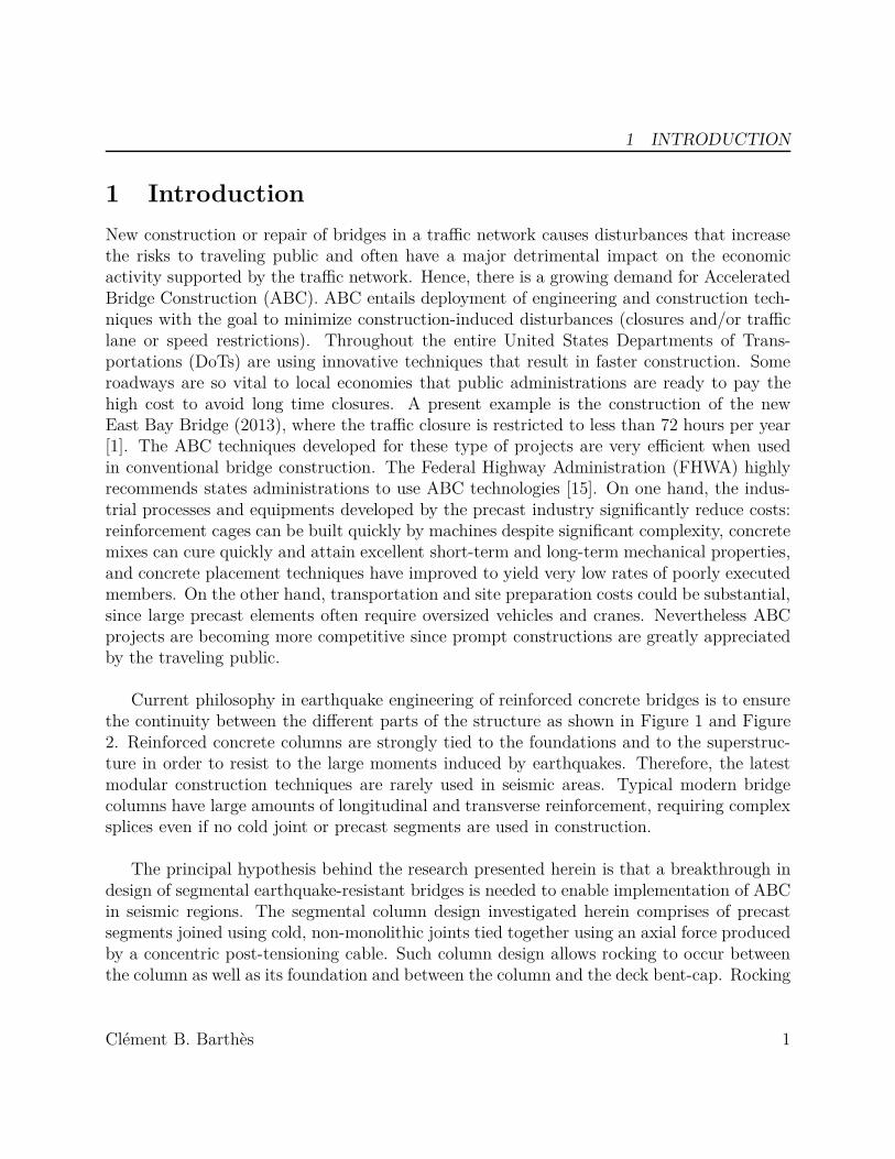
1 IntroductionNew construction or repair of bridges in a traffic network causes disturbances that increasethe risks to traveling public and often have a major detrimental impact on the economicactivity supported by the traffic network. Hence, there is a growing demand for AcceleratedBridge Construction (ABC). ABC entails deployment of engineering and construction tech-niques with the goal to minimize construction-induced disturbances (closures and/or trafficlane or speed restrictions). Throughout the entire United States Departments of Trans-portations (DoTs) are using innovative techniques that result in faster construction. Someroadways are so vital to local economies that public administrations are ready to pay thehigh cost to avoid long time closures. A present example is the construction of the newEast Bay Bridge (2013), where the traffic closure is restricted to less than 72 hours per year[1]. The ABC techniques developed for these type of projects are very efficient when usedin conventional bridge construction. The Federal Highway Administration (FHWA) highlyrecommends states administrations to use ABC technologies [15]. On one hand, the indus-trial processes and equipments developed by the precast industry significantly reduce costs:reinforcement cages can be built quickly by machines despite significant complexity, concretemixes can cure quickly and attain excellent short-term and long-term mechanical properties,and concrete placement techniques have improved to yield very low rates of poorly executedmembers. On the other hand, transportation and site preparation costs could be substantial,since large precast elements often require oversized vehicles and cranes. Nevertheless ABCprojects are becoming more competitive since prompt constructions are greatly appreciatedby the traveling public.
Current philosophy in earthquake engineering of reinforced concrete bridges is to ensurethe continuity between the different parts of the structure as shown in Figure 1 and Figure2. Reinforced concrete columns are strongly tied to the foundations and to the superstruc-ture in order to resist to the large moments induced by earthquakes. Therefore, the latestmodular construction techniques are rarely used in seismic areas. Typical modern bridgecolumns have large amounts of longitudinal and transverse reinforcement, requiring complexsplices even if no cold joint or precast segments are used in construction.
The principal hypothesis behind the research presented herein is that a breakthrough indesign of segmental earthquake-resistant bridges is needed to enable implementation of ABCin seismic regions. The segmental column design investigated herein comprises of precastsegments joined using cold, non-monolithic joints tied together using an axial force producedby a concentric post-tensioning cable. Such column design allows rocking to occur betweenthe column as well as its foundation and between the column and the deck bent-cap. Rocking
Clément B. Barthès 1

1 INTRODUCTION
Figure 1: Typical multi-span California standard ordinary bridge
may even occur between the column segments along the column height. Close attention isgiven to rocking behavior; instead of preventing or limiting it, it is proposed to use rockingbehavior as an energy dissipation and seismic isolation mechanism in bridge columns. Suchseismic response modification technique is expected to enable ABC as well as to enhancethe seismic performance of bridges, ushering in the next generation of earthquake-resistantbridge design.
In Chapter 2, modular construction techniques for seismic resistant bridges are presented.In particular, design solutions allowing monolithic connections between precast elements arediscussed. Currently, large parts of the structure are often cast in place in order to ensurethe continuity of the concrete reinforcements. So it is propoosed to consider a new designapproach, allowing discontinuity between precast elements.
In Chapter 3, a literature review for the behavior of rigid blocks subjected to rocking ispresented. It is then proposed to restrain a rigid block with an unbonded post-tensioningcable in order to allow rocking but prevent overturning.
Clément B. Barthès 2

1 INTRODUCTION
Figure 2: Monolithic design of a standard ordinary bridge
In Chapter 4, the implementation of a finite element capable of representing rocking ispresented. This element can be used in combination with existing prismatic elements, allow-ing it to model very complex deformable structures with multiple rocking surfaces. Specificissues concerning the handling of the discontinuous constraints by the computational algo-rithm are discussed.
In Chapter 5, the rocking element developed in the previous chapter is used to investigatethe interaction between rocking and elastic deformation. Issues concerning the implementa-tion of the viscous damping are discussed and the rocking termination due to column bendingis also investigated.
In Chapter 6, the stability of a deformable rocking column subjected to an earthquakeground motion is studied. For a severe earthquake, the restraining cable may fail and leadto collapse. Therefore, it is proposed to use a mild-steel fuse at the base of the column inorder to dissipate energy during the earthquake excitation.
In Chapter 7, it is proposed to compare the seismic response of a conventional monolithicbridge with the response of a bridge with columns allowed to rock at both ends. Severalbridge configurations are investigated. Notably, the rocking behavior of a multi-span bridgewhose columns have a different aspect ratio is investigated. The benefits of a dissipative fuseare also investigated.
At last in Chapter 8, the findings made during this Ph.D. are summarized. Several rec-ommendations for further research, including the implementation of a 3D rocking element,are presented.
Clément B. Barthès 3

2 MODULAR BRIDGE CONSTRUCTION
2 Modular Bridge Construction
2.1 IntroductionNearly eighty percent of Californian highway bridges are cast-in-place post-tensioned con-crete bridges designed and developed using engineering techniques of the 1980’s and 1990’s.Great effort has been made in the last few decades to increase safety concerning earthquakehazards, in particular. Today, Californian highway bridges are safe. They fulfill strict seismicsafety standards prescribed in Caltrans Seismic Design Criteria [3].
Meanwhile, modular bridge construction techniques have greatly improved over the lastdecades. Many departments of transportation tend to avoid cast-in-place (CIP) concrete asmuch as possible for several reasons. First of all, it induces larger environmental impact onthe construction site and a large quantity of concrete may be wasted due to late deliveryor over production. Second, the quality of the precast concrete has greatly improved overthe last few decades. A compressive strength 50% higher than CIP concrete can easily beobtained with modern curing process. Modular construction also allows faster and cheaperconstructions. Costs can be greatly reduced when segments are built with modern industrialprocesses during both module construction and module on-site assembly.
The principal advantage is that the modular construction accelerates construction for de-sign and building of the next generation highway overpass bridges. However, ABC is rarelyused in seismic areas because of the perceived weakness of the connections between the el-ements. Typically, a column of a bridge designed to provide high seismic resistance andsatisfactory seismic performance is designed with substantial continuous longitudinal andtransversal reinforcement. It is strongly anchored in the footing and the bridge deck andparticular attention is given to the reinforcement splices. Such reinforcement continuity isnot achievable with precast concrete elements unless large amounts of cast-in-place concreteare used. In some cases, these prefabricated elements simply consist of reinforced concrete,steel, glass, carbon fiber, or even polymer shells and are capable of resisting the hydraulicforces of the cast-in-place concrete. However, the DoTs use more and more entirely precastelements and only the connections are cast-in-place.
The purpose of this chapter is to present the review of column construction and connectiontechniques with respect to their use in ABC and their capability to meet seismic safetystandards.
Clément B. Barthès 4

2 MODULAR BRIDGE CONSTRUCTION
2.2 Existing Precast Elements ConnectionsConventional design of segmental bridges comprised of prefabricated elements (steel or con-crete) is predicated on the rigidity (ability to transfer moments, shears and axial forceswithout deformation) or semi-rigidity of column connections to the foundation and the super-structure. The heavy mass of the superstructure generates a lateral force at the top of thecolumn. If the connection between the column and the superstructure behaves as a pin,the column is loaded as a cantilever; as a result, a substantial demand on the foundations.Therefore, it is preferred to clamp the column and the bent-cap together, preventing the topof the column to rotate and reducing the moment at the base, as shown in Figure 3.
Moment Moment
Figure 3: The moment at the base of the column is reduced when the rotation is locked atthe top
This rule is easy to apply to cast-in-place structures but specific joints are required forapplying it to prefabricated structures. It is difficult to drastically reduce the cast-in-placeconcrete volume and ensure monolithic junctions. The columns can be delivered with stand-by reinforcements on both ends, allowing for monolithic connection with the footing and thesuperstructure. Figure 4 shows an example of the installation of a precast bent-cap over aprecast column in Texas. But if the columns exceed 100ft, it is inconceivable to use fullprecast columns.
If the column has to be segmented, then the splices between the longitudinal reinforce-ments become too complicated; therefore, it is more reasonable to go for a permanent form-work system to ensure a correct shear resistance. A new design is now used in Japan calledSumitumo Precast form for Resisting Earthquake and for Rapid construction (SPER) [29],shown in figures 5 and 6. This system is made to use the precast element as both permanentformworks and structural elements. There are two versions of the product, for piers up to40ft the square sections are delivered with cross ties already installed. They are stacked on
Clément B. Barthès 5

2 MODULAR BRIDGE CONSTRUCTION
Figure 4: Precast Bent-Cap Installed on Site (Texas DOT)
top of each other using epoxy glue along the vertical reinforcements. The concrete is thencast inside the pier to give a solid section. The cross-ties inside the forms give enough lateralresistance to the panels to resist to the pressure while pouring the concrete, so it does notrequire any temporary shoulder during the construction. The time saved with this techniquecompared to an entirely cast-in-place system is 50%.
Figure 5: SPER System for Solid Section Columns [29]
The second version of the product is designed for higher piers, up to 160 ft. It is a hollowsection where both inner and outer formworks are permanent structural elements. They aresegmented in half-sections to reduce size for hauling. They are placed around the verticalreinforcements and then connected using couplers. The cross ties also have to be installed onsite, then the concrete is poured. The time saved compared to a traditional technique is 30%.
Clément B. Barthès 6

2 MODULAR BRIDGE CONSTRUCTION
Figure 6: SPER System for Hollow Section Columns [29]
Clément B. Barthès 7
2 MODULAR BRIDGE CONSTRUCTION
2.2.1 Grouted Pockets
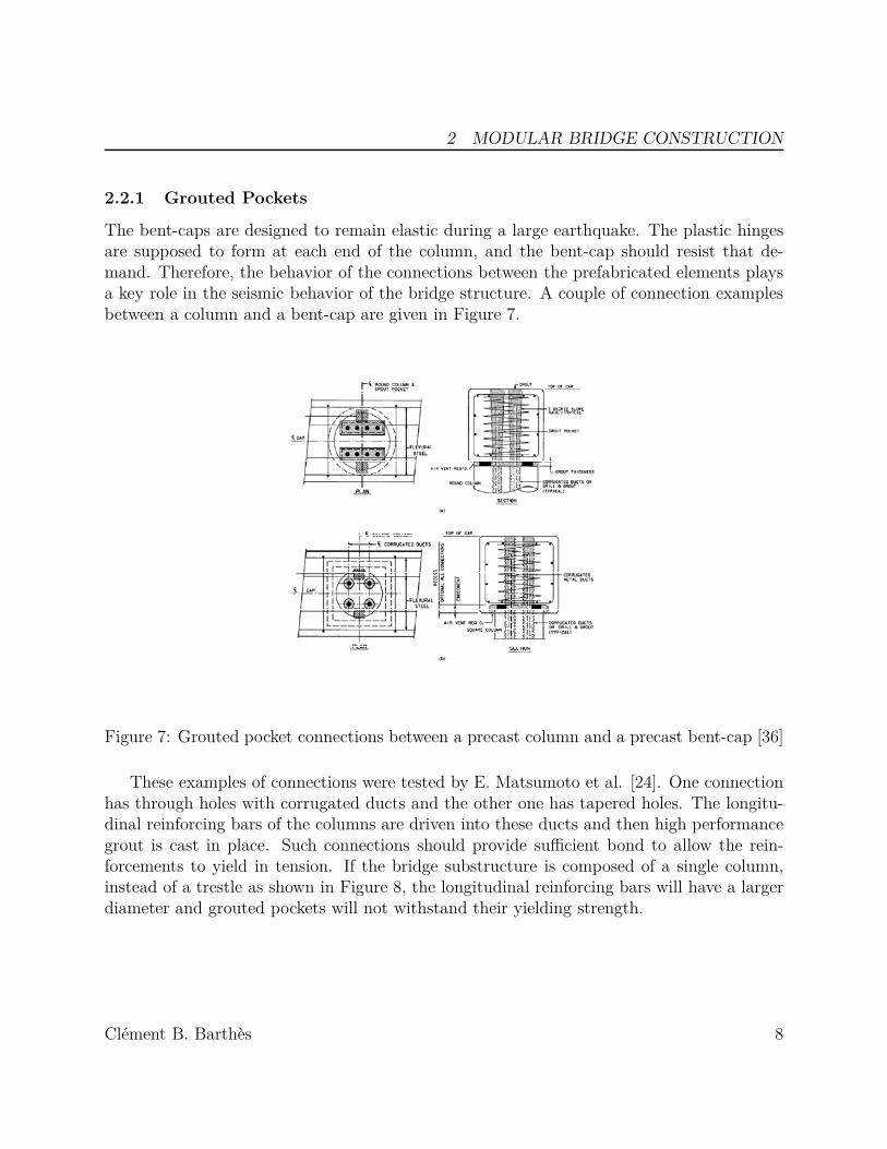
The bent-caps are designed to remain elastic during a large earthquake. The plastic hingesare supposed to form at each end of the column, and the bent-cap should resist that de-mand. Therefore, the behavior of the connections between the prefabricated elements playsa key role in the seismic behavior of the bridge structure. A couple of connection examplesbetween a column and a bent-cap are given in Figure 7.
Figure 7: Grouted pocket connections between a precast column and a precast bent-cap [36]
These examples of connections were tested by E. Matsumoto et al. [24]. One connectionhas through holes with corrugated ducts and the other one has tapered holes. The longitu-dinal reinforcing bars of the columns are driven into these ducts and then high performancegrout is cast in place. Such connections should provide sufficient bond to allow the rein-forcements to yield in tension. If the bridge substructure is composed of a single column,instead of a trestle as shown in Figure 8, the longitudinal reinforcing bars will have a largerdiameter and grouted pockets will not withstand their yielding strength.
Clément B. Barthès 8

2 MODULAR BRIDGE CONSTRUCTION
Figure 8: Trestle Type Prefabricated Concrete Columns [36]
Clément B. Barthès 9

2 MODULAR BRIDGE CONSTRUCTION
2.2.2 Self-Compacting Concrete
The mechanical properties of Self-Compacting Concrete (SCC) are the same as conventionalconcrete. However, SCC is less sensitive to the casting process, so if the concrete is correctlytested when it is delivered, its strength and its compaction are almost insensitive to humanerrors such as over vibration. For conventional concrete, the flowing ability is increased byadding water, but this reduces the mechanical properties. But for SCC, the flowing ability isgiven by superplasticisers. The cohesiveness is usually insured by high powder contents suchas ground granulated blast furnace slag, fly ash and other fine inert materials. At similar wa-ter/cement ratios, the strength of SCC is equal or slightly better than conventional concrete.Compressive strength between 5 and 10 ksi can easily be achieved. When delivered, the SCCrequires more tests than a conventional concrete, so the foremen need to be trained to usethis new material. Since the SCC can be pumped to the formworks and simply poured, littleor no vibration is required, so the task for the workers is easier. SCC is used to reduce costsin various projects. It is because the process is faster but also because the surface does notneed any other treatment or finish. Because it is mainly constituted of fine granulates, itis easy, for example to incorporate an esthetic pattern in the formworks. SCC is used forurban construction to reduce noises. It is a key element to run a quiet construction andallows night work. For example, it is now common to prepare formworks during daytime,and then schedule most of the casting during night time. In addition to saving time, it alsoavoids concrete trucks blocking the area near the construction site.
Figure 9: Self-Compacting Concrete being cast
The principal use of SCC in ABC is to implement the monolithic (pocket-type or othertypes) connections between pre-cast segments. Since all the reinforcements have to be spliced,
Clément B. Barthès 10

2 MODULAR BRIDGE CONSTRUCTION
it requires a high density of reinforcements at the connection as shown in Figure 10. Due toits flowing ability, SCC allows to cast in place integral connections between two prefabricatedelements.
Figure 10: Congested Reinforcements
Clément B. Barthès 11

2 MODULAR BRIDGE CONSTRUCTION
2.3 Bridge Columns With Unbonded SegmentsSegmental construction of bridge columns in seismic areas constituted the main incentivefor the research presented below. Current practice consists of bonding the different elementswith adequate reinforcement splicing. But these splices limit the use of precast elements.The column reinforcements can be bonded to the bent-cap with grouted pockets as shown inFigure 7 but, even with properly designed corrugated grouted pockets, slipping is observedat ultimate capacity.
Figure 11: Monolithic Bridge Substructure Assembly Subjected to Earthquake Motion
Figure 11 shows the behavior of a Californian bridge substructure subjected to earth-quake motion. It consists of a continuous structure with column connections capable oftransferring shear and moment to the footing and the superstructure. On the contrary, seg-mental bridge construction technique simply consists of stacking the column elements witha cold, grouted or ungrouted, joint. Such simple design would lead to rocking and slippingbetween the elements when subjected to a severe earthquake. However, it is believed thata post-tensioning cable may be able to prevent slipping and limit rocking to reasonable ro-tations. Furthermore, the rocking between the different elements may be beneficial for thebridge. Rocking dissipates energy through shock wave radiation and it also modifies theresponse of the structure, making it less sensitive to earthquake excitations in some cases.
Clément B. Barthès 12

2 MODULAR BRIDGE CONSTRUCTION
Figure 12 shows the expected behavior of an unbonded segmented column.
Figure 12: Unbonded Segmented Bridge Substructure Subjected to Earthquake Motion
The behavior of rigid blocks rocking on their base is inherently unstable, so designershave been trying to prevent it. It was only after Housner [16], who observed that some watertanks resisted a major earthquake in Chile, likely due to their rocking behavior, that researchwas led on this subject. Recently, a lot of studies were done on rocking shear walls. M.R.Eatherton et al. [8] tested a rocking shear wall with a special fuse on the E-Defense shaketable in Japan. Some structures allowing a frame to rock were even recently built, such asthe Orinda City Hall [23].
Figure 13: Cylinder Rocking
In order to use rocking in earthquake resistant bridge design, the fundamentals of rockingrigid body have to be well understood. The dynamic behavior of rocking blocks induces shock
Clément B. Barthès 13

2 MODULAR BRIDGE CONSTRUCTION
waves, so the quasi-static approach often used in civil engineering may not be sufficient.Chapter 3 covers the dynamics of rocking rigid blocks, required to assess the integrity ofsegmented columns. A particular attention will be given to the instability issue and asolution will be proposed using post-tensioning cable.
Clément B. Barthès 14
2 MODULAR BRIDGE CONSTRUCTION
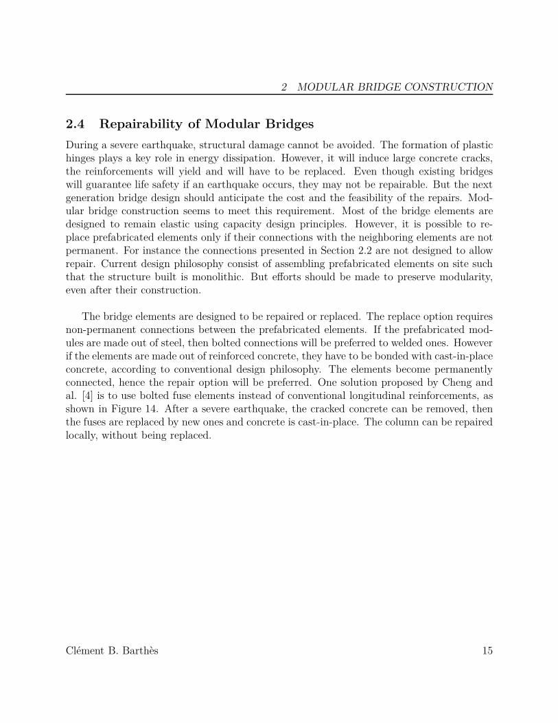
2.4 Repairability of Modular BridgesDuring a severe earthquake, structural damage cannot be avoided. The formation of plastichinges plays a key role in energy dissipation. However, it will induce large concrete cracks,the reinforcements will yield and will have to be replaced. Even though existing bridgeswill guarantee life safety if an earthquake occurs, they may not be repairable. But the nextgeneration bridge design should anticipate the cost and the feasibility of the repairs. Mod-ular bridge construction seems to meet this requirement. Most of the bridge elements aredesigned to remain elastic using capacity design principles. However, it is possible to re-place prefabricated elements only if their connections with the neighboring elements are notpermanent. For instance the connections presented in Section 2.2 are not designed to allowrepair. Current design philosophy consist of assembling prefabricated elements on site suchthat the structure built is monolithic. But efforts should be made to preserve modularity,even after their construction.
The bridge elements are designed to be repaired or replaced. The replace option requiresnon-permanent connections between the prefabricated elements. If the prefabricated mod-ules are made out of steel, then bolted connections will be preferred to welded ones. Howeverif the elements are made out of reinforced concrete, they have to be bonded with cast-in-placeconcrete, according to conventional design philosophy. The elements become permanentlyconnected, hence the repair option will be preferred. One solution proposed by Cheng andal. [4] is to use bolted fuse elements instead of conventional longitudinal reinforcements, asshown in Figure 14. After a severe earthquake, the cracked concrete can be removed, thenthe fuses are replaced by new ones and concrete is cast-in-place. The column can be repairedlocally, without being replaced.
Clément B. Barthès 15

2 MODULAR BRIDGE CONSTRUCTION
Figure 14: Bolted Longitudinal Reinforcements [4]
The prefabricated column elements studied in this thesis have discontinuous reinforce-ments. They are assembled on site with a simple joint of grout and the flexural resistance ofthe column comes from the post-tensioning cables. Such design may allow DoTs to replacedamaged elements after a severe earthquake if the post-tensioning cable remains unbonded.But such structure will behave differently than current standard ordinary bridges underearthquake loading. The grouted joints will fail, allowing rocking between the elements.New design guidelines have to be made, and the cables must allow the substructure to re-main stable.
Clément B. Barthès 16
3 RIGID BLOCKS SUBJECTED TO ROCKING
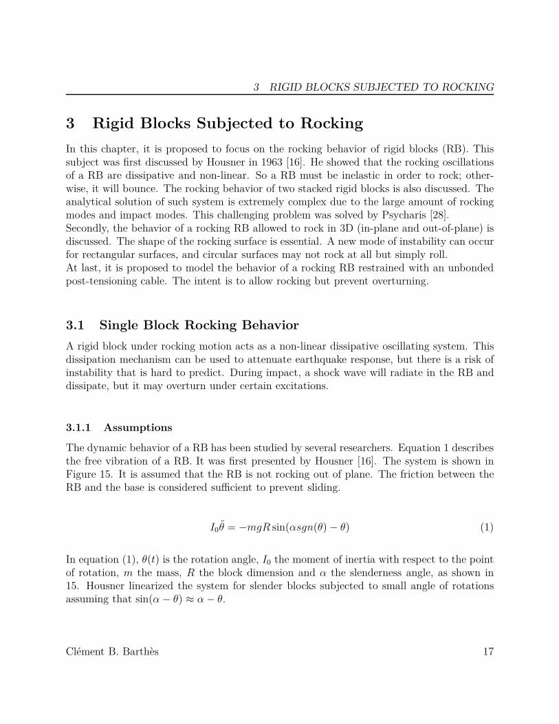
3 Rigid Blocks Subjected to RockingIn this chapter, it is proposed to focus on the rocking behavior of rigid blocks (RB). Thissubject was first discussed by Housner in 1963 [16]. He showed that the rocking oscillationsof a RB are dissipative and non-linear. So a RB must be inelastic in order to rock; other-wise, it will bounce. The rocking behavior of two stacked rigid blocks is also discussed. Theanalytical solution of such system is extremely complex due to the large amount of rockingmodes and impact modes. This challenging problem was solved by Psycharis [28].Secondly, the behavior of a rocking RB allowed to rock in 3D (in-plane and out-of-plane) isdiscussed. The shape of the rocking surface is essential. A new mode of instability can occurfor rectangular surfaces, and circular surfaces may not rock at all but simply roll.At last, it is proposed to model the behavior of a rocking RB restrained with an unbondedpost-tensioning cable. The intent is to allow rocking but prevent overturning.
3.1 Single Block Rocking BehaviorA rigid block under rocking motion acts as a non-linear dissipative oscillating system. Thisdissipation mechanism can be used to attenuate earthquake response, but there is a risk ofinstability that is hard to predict. During impact, a shock wave will radiate in the RB anddissipate, but it may overturn under certain excitations.
3.1.1 Assumptions
The dynamic behavior of a RB has been studied by several researchers. Equation 1 describesthe free vibration of a RB. It was first presented by Housner [16]. The system is shown inFigure 15. It is assumed that the RB is not rocking out of plane. The friction between theRB and the base is considered sufficient to prevent sliding.
I0θ = −mgR sin(αsgn(θ) − θ) (1)
In equation (1), θ(t) is the rotation angle, I0 the moment of inertia with respect to the pointof rotation, m the mass, R the block dimension and α the slenderness angle, as shown in15. Housner linearized the system for slender blocks subjected to small angle of rotationsassuming that sin(α − θ) ≈ α − θ.
Clément B. Barthès 17

3 RIGID BLOCKS SUBJECTED TO ROCKING
Figure 15: Description of the Rocking Block
The RB behavior can be described with only two parameters p and α, leading to equation(2), where p[1/sec] represents the frequency parameter of the system. This parameter canbe compared to the natural frequency parameter describing harmonic oscillator, ωn. As pgets larger, the free rocking oscillations frequency of a RB will be higher. Free harmonicoscillations periods can be quickly computed with ωn , but there is no simple interpretationof p to determinate the behavior of a rocking RB. For the case of a rectangular block, thefrequency parameter is p =
√3g/4R.
θ = −p2{sin(αsgn(θ(t)) − θ(t)) +ug(t)
gcos(αsgn(θ(t)) − θ(t))} (2)
α plays a major role in the energy dissipation of the system as described below. Toincorporate the energy dissipation at the impact, Housner [16] assumed that the rotationcontinues smoothly from point O to O′ (no sliding) and that the angular momentum duringthe impact is conserved (see Figure 15). The relationship between the angular velocities isobtained by applying the conservation of angular momentum. The coefficient of restitutionr of the impact can be computed as shown in equation (3). A confusion sometimes occursconcerning the balance of angular momentum. During an impact, the angular momentumis not conserved for the RB but for the RB-footing system. Similarly, the linear momentumof the RB is not conserved but the linear momentum of the RB-footing system is conserved.Since the footing has an infinite mass, the conservation of momentum at impact of the RB-footing system can not be computed. However, the impact between the RB and the footingis assumed to be a point impact. Therefore, the RB is subjected to a rolling constraint andcan not have a reaction moment at the point of impact. Hence the angular momentum isconserved for the RB alone. If a RB is rocking on an isolated base with a finite mass, then
Clément B. Barthès 18

3 RIGID BLOCKS SUBJECTED TO ROCKING
−1 −0.8 −0.6 −0.4 −0.2 0 0.2 0.4 0.6 0.8 1−0.2
−0.15
−0.1
−0.05
0
0.05
0.1
0.15
0.2
θ/α
M/M
0
Figure 16: Moment vs. rotation of a RB
the conservation of linear momentum and angular momentum must be conserved for theRB-base system, as explained by Vassiliou and Makris [35].
r =(
θ2
θ1
)2
=(
1 − 32
sin2 α)2
(3)
Figure 16 represents the moment versus the rotation of a RB. Once the excitation reachesthe required magnitude to initiate rocking, the RB becomes unstable since the resisting mo-ment due to the RB weight decreases as θ increases.
Equation (3) implies that a slender RB looses less energy than squat ones; therefore, thedamping ratio depends on the RB slenderness α. Due to dissipation of angular momentumduring impact (radiation damping into the RB and the base), the vibration period of sub-sequent cycles decreases. The horizontal acceleration required to initiate rocking is definedby equation (4).
ugmin
g≥ tan(α) (4)
Housner [16] also studied the overturning of a RB subjected to constant horizontal ac-celeration, to sine pulse, and to earthquake type of excitation. He concluded that for twogeometrically similar blocks the scale effect makes the larger (i:e. with a smaller p) morestable than the smaller. This scale effect is shown in Figure 17. Since the rocking initiation
Clément B. Barthès 19

3 RIGID BLOCKS SUBJECTED TO ROCKING
only depends on α, it is important to notice that RBs of identical slenderness but withdifferent sizes will start to rock under the same excitation magnitude. However, the largerones will be more stable.
Finally, Shenton [32] studied the initiation of rocking and sliding for a RB subjected tobase excitation. He showed that a slide-rock mode may exist when the friction coefficientof a rocking RB is smaller than its friction coefficient at rest. However, this mode can onlyoccur for α ≤ π/4.
Clément B. Barthès 20

3 RIGID BLOCKS SUBJECTED TO ROCKING
Figure 17: Response of RBs with α = 25◦ to a Half-Cosine Ground Acceleration Pulse ofAmplitude 0.61g and Period T = 2sec
Clément B. Barthès 21

3 RIGID BLOCKS SUBJECTED TO ROCKING
3.1.2 SDOF Vibration Analogy
Priestley et al. [27] proposed a design methodology to estimate RB rotations when sub-jected to earthquake horizontal excitation. The method consists of transforming the RB toan equivalent single-degree-of-freedom (SDOF) system with a period and viscous damping.The maximum rotation angle is computed from δ = θR cos(α), where δ is the displacementof the centroid of the block, which is obtained from a response spectrum of a SDOF sys-tem. To define the equivalent viscous damping of a RB system, the relationship between therotation amplitude in subsequent cycles is used. The equivalent period of the RB dependson the maximum rotation angle θ; therefore, this methodology requires an iteration process.The idea presented by Priestley is used by FEMA 356 [10], but it uses conservatively a lowerdamping ratio.
From their study, Makris and Konstantinidis [22] concluded that the SDOF oscillatorand the RB are two fundamentally different systems. For example, the free vibration of aRB is characterized by an increase of the frequency and a decrease of amplitude. On thecontrary, a SDOF oscillator vibrates with constant frequency. Therefore, the response of oneof these two systems should not be used to predict the behavior of the other. Additionally,they concluded that the approximate design methodology to estimate block rotations imple-mented in FEMA 356 is conceptually wrong and should be abandoned.
Makris and Konstantinidis [22] focused their attention in solving the nonlinear dynamicequation of a RB subjected to horizontal ground acceleration. The equation of motion of arigid block subjected to ground acceleration ug(t) is written in equation (2). J. Zhang andN. Makris [37] focused on the effect of cyclic loadings on rocking structures.
Clément B. Barthès 22

3 RIGID BLOCKS SUBJECTED TO ROCKING
3.1.3 Rocking termination
It is often assumed that rocking oscillations vanish but do not stop, similar to a harmonicoscillator with viscous damping. But, unlike a damped harmonic oscillator, when the ampli-tude of a rocking RB decreases, the period of rocking oscillations also decreases. Therefore,the rapid decay of the period may cause rocking interruption at a finite time.
Housner [16] did not elude this question. Instead, he stated that after a few impacts therocking amplitude becomes so small that other phenomenon such as elastic bouncing willcause rocking to stop. It is proposed in this section to prove that rocking will stop at a finitetime, even for a perfectly rigid block.
In order to compute the time of the free rocking response, the equation of motion (2) islinearized. Housner [16] linearized this equation for α − θ but in this section, the equationof motion is linearized only for θ, while the slenderness angle α is still considered large. Thelinearized equation is presented in Equations (5a) and (5b).
θ − p2 cos(α) · θ + o(θ2) = −p2 sin(α) for θ > 0 (5a)θ − p2 cos(α) · θ + o(θ2) = p2 sin(α) for θ < 0 (5b)
Equations (6a) and (6b) represent the solution of Equation (5a) for θ(0) = θ0 (withθ0 > 0) and θ(0) = 0. A new frequency parameter is defined as p = p
√cos(α).
θ(t) = tan(α) − (tan(α) − θ0) · cosh(pt) (6a)θ(t) = −(tan(α) − θ0) · p · sinh(pt) (6b)
After the n-th impact, the maximum rotation is defined as θn. The angular velocity atimpact n is defined as θn. At the time of the n-th impact defined as tn, Equation (6a) canbe expressed as Equation (7).
0 = tan(α) − (tan(α) − θn−1) · cosh(ptn) (7)
Clément B. Barthès 23

3 RIGID BLOCKS SUBJECTED TO ROCKING
Using the hyperbolic function identity cosh2 x + sinh2 x = 1, Equation (7) leads to Equa-tion (8).
cosh(ptn) = tan(α)tan(α) − θn−1
=⇒ sinh(ptn) =
√√√√(tan(α)
tan(α) − θn−1
)2
− 1 (8)
Therefore, the angular velocity at impact n is:
θn = p ·√
tan2(α) − (tan(α) − θn−1)2 (9)
The coefficient of restitution r defined in Equation (3) leads to the recursive Equation10 between the angular velocity at impact n and the angular velocity at impact n − 1.
p ·√
tan2(α) − (tan(α) − θn)2 = p · √r ·
√tan2(α) − (tan(α) − θn−1)2 (10)
Hence the maximum rotation after impact n can be expressed as:
θn = tan(α) −√
tan2(α) − rn (tan2(α) − (tan(α) − θ0)2) (11)
The quarter period Tn/4 is defined as the duration between the time tn at which therotation reaches its maximumn after impact n and the time at impact tn+1. Equation (7) isexpressed as a function of tn + Tn
4 in Equation (12).
0 = tan(α) − (tan(α) − θn) · cosh(p(tn + Tn
4)) (12)
Combining Equation (10) and Equation (12), the time at impact n + 1 is expressed inEquation (13) with respect to the time at impact n. Note that there are two quarter periodsTn/4 between two impacts.
tn+1 = tn + 2p
√√√√√rn
⎡⎣1 −
(tan(α) − θ0
tan(α)
)2⎤⎦ (13)
Clément B. Barthès 24

3 RIGID BLOCKS SUBJECTED TO ROCKING
Due to the recursivity of Equation (13), the total time of the free rocking motion can beexpressed in Equation (14).
t∞ =2p
√√√√1 −(
tan(α) − θ0
tan(α)
)2
·∞∑
n=0
(√r)n
(14)
Based on the definition of the reduction factor, for any α, r < 1. Hence Equation (14)converges and leads to Equation (15).
t∞ =2p
√√√√1 −(
tan(α) − θ0
tan(α)
)2
· 11 − √
r(15)
The equation of motion was linearized with respect to θ and, since the initial angle θ0is finite, the time of rocking interruption t∞ is approximate. However, this demonstrationproves that the free rocking response of a rigid block will lead to an infinite number of im-pacts but it will stop at a finite time for any slenderness angle α.
Clément B. Barthès 25

3 RIGID BLOCKS SUBJECTED TO ROCKING
3.2 3D Rocking BlockIn this section, the RB is allowed to rock on a flat surface in any direction, as described inFigure 18. It is still assumed that the RB does not slide and always remains in contact withthe base. The rocking behavior in 3D is largely dependent of the shape of its base. It canbe subdivided into two categories: the RB with a polygonal base and the RB with a circularbase.
Figure 18: Rolling of a Cylinder on Its Edge (From [33])
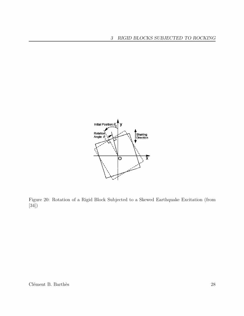
After Sanriku-Haruka-Oki earthquake in 1994, Tobita and Sawada [34] noticed that slen-der granite tombstones were rotated. A sliding block subjected to earthquake excitation maytranslate but should not rotate so noticeably. Hence it was concluded that the tombstonesrotated because of rocking. The multi-directional excitation of an earthquake caused thetombstone to rock in its two transverse directions. Incidentally, the RB was not rocking onits edge but on its corner, allowing it to rotate.
Tobita and Sawada conducted experiments on a shaking table with rigid blocks subjectedto skewed earthquake excitations as shown in Figure 20. Once the block uplifts on its corner,it tends to twist around one corner until the center of rotation and the center of gravity arealigned with the excitation, leading to the curious disposition of the tombstone after theearthquake.
The rocking behavior of a cylinder was studied by Srinivasan and Ruina [33]. The cylin-der is considered rigid, and its bottom edge is constrained to remain in contact with thesupporting surface, as shown in Figure 18. The friction is considered sufficient to prevent
Clément B. Barthès 26

3 RIGID BLOCKS SUBJECTED TO ROCKING
Figure 19: Tombstone Rotated After Sanriku-Haruka-Oki Earthquake (1994)
sliding. It is shown that the cylinder will not rock but will instead roll. Unlike the 2D case,there is no impact between the cylinder and the support. If the cylinder is initially tiltedand no angular velocity is applied along its longitudinal axis, it will bifurcate to the left orto the right and roll on its edge. Hence a rocking cylinder is, in fact, only rolling.
In conclusion, 3D rocking motions have two properties unobserved in 2D. One is that theytend to rotate when they have a polygonal base and the other is that they no longer rock butsimply roll when they have a circular base. If only rolling occurs, there is no dissipation dueto the absence of impacts. A compromise may be found by using a polygonal base with tan-gent rounded edges; if the block is rocking on one edge then impacts can occur, if it is rockingon a corner, then it rolls until it reaches an edge. This configuration has not yet been studied.
Clément B. Barthès 27
3 RIGID BLOCKS SUBJECTED TO ROCKING
Figure 20: Rotation of a Rigid Block Subjected to a Skewed Earthquake Excitation (from[34])
Clément B. Barthès 28

3 RIGID BLOCKS SUBJECTED TO ROCKING
3.3 Two-block Rocking AssembliesPsycharis [28] derived the equations of motions for two-block assemblies. It is assumed thatthe blocks are rigid and that no sliding occurs. As shown in Figure 21, the upper blockcan rock on top of the lower block. The system is inherently less stable than a single block.For instance, if only the lower block is rocking, the upper block may overturn before it evenstarts to rock if it is more slender than the lower block.
Figure 21: 2 Rigid Blocks Assembly (from [28])
Four different rocking motion modes may occur, as shown in Figure 22. These modescan be described by eight systems of linear dynamic equations, each mode being governedby two different systems of equations, whether the rocking rotations are positive or negative.Furthermore, six equations govern the transition from one mode to the other to conservethe angular momentum, and eight equations govern the initiation of the rocking modes. Inorder to solve these sets of ODEs, the algorithm must detect each event and then convergeto it. Transition equations are solved for the solution of the previous ODE and applied tothe new ODE system as initial values, as explained in 3.4.1.
Psycharis computed the solution for a free rocking assembly and for an assembly sub-jected to an earthquake excitation. It shows that, if the structure does not overturn, theenergy is redistributed to the upper block which is therefore subjected to larger rotations.
Clément B. Barthès 29

3 RIGID BLOCKS SUBJECTED TO ROCKING
Figure 22: Rocking Modes for 2 Blocks Assemblies (from [28])
As shown in Figure 23, the rotations of the lower block vanish very quickly and the systemquickly turns into a single block rocking response of the upper block.
In order to study the behavior of multiple stacked rigid blocks, a numerical method calledthe distinct element method was used by Konstantinidis and Makris [19].
Clément B. Barthès 30

3 RIGID BLOCKS SUBJECTED TO ROCKING
0 0.5 1 1.5 2 2.5 3 3.5 4 4.5 5−0.15
−0.10
−0.05
0
0.05
0.1
0.15
Time [sec]
φ 2 [rad
]
Top RB
0 0.5 1 1.5 2 2.5 3 3.5 4 4.5 5−0.15
−0.1
−0.05
0
0.05
0.1
0.15
Time [sec]
φ 1 [rad
]
Bottom RB
Figure 23: Free Rocking Response of a Two Rigid Blocks Assembly (from [28])
Clément B. Barthès 31
3 RIGID BLOCKS SUBJECTED TO ROCKING
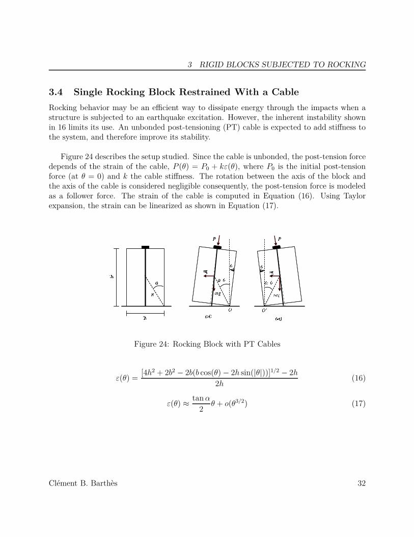
3.4 Single Rocking Block Restrained With a CableRocking behavior may be an efficient way to dissipate energy through the impacts when astructure is subjected to an earthquake excitation. However, the inherent instability shownin 16 limits its use. An unbonded post-tensioning (PT) cable is expected to add stiffness tothe system, and therefore improve its stability.
Figure 24 describes the setup studied. Since the cable is unbonded, the post-tension forcedepends of the strain of the cable, P (θ) = P0 + kε(θ), where P0 is the initial post-tensionforce (at θ = 0) and k the cable stiffness. The rotation between the axis of the block andthe axis of the cable is considered negligible consequently, the post-tension force is modeledas a follower force. The strain of the cable is computed in Equation (16). Using Taylorexpansion, the strain can be linearized as shown in Equation (17).
Figure 24: Rocking Block with PT Cables
ε(θ) = [4h2 + 2b2 − 2b(b cos(θ) − 2h sin(|θ|))]1/2 − 2h
2h(16)
ε(θ) ≈ tan α
2θ + o(θ3/2) (17)
Clément B. Barthès 32

3 RIGID BLOCKS SUBJECTED TO ROCKING
Figure 25: Strain in the Post-Tensioning Cable for θ = α
Clément B. Barthès 33

3 RIGID BLOCKS SUBJECTED TO ROCKING
Figure 25 shows that the strain can be considered linear, especially for slender blocks.Based on this assumption, the post-tension force can be represented by two dimensionlessparameters, η0 and ηα as shown in equation (18). η0 represents the initial post-tension forceat θ = 0 (divided by the weight) and ηα represents the post-tension force when the PT-RBreaches angle θ = α. Hence, if a cable is very soft, the post-tension force remain constantduring motion and η0 = ηα. The balance of angular moment with respect to O and O′ leadsto Equations (19a) and (19b).
P (θ) = mg(η0 + (ηα − η0) θ
α) (18)
I0θ = −P (θ)R sin(α) − mugR cos(α − θ) − mgR sin(α − θ)for θ > 0 (19a)I0θ = P (θ)R sin(α) − mugR cos(α − θ) − mgR sin(−α − θ)for θ < 0 (19b)
Combining equations (18) and (19) leads to equation (20).
θ = −p2{sin(αsign(θ)−θ)+ ug(t)g
cos(αsign(θ)−θ)+(η0sign(θ)+(ηα −η0) θ
α) sin(α)} (20)
The energy dissipation is incorporated at each impact using the conservation of angularmomentum given by equation (3). Therefore, the post-tension cable is assumed to remainelastic and it does not dissipate energy. For a PT-RB, the minimum ground accelerationrequired to initiate rocking depends only on η0. The required acceleration to initiate rockingis defined in equation (21). Compared to Equation (4), the effect of the PT cable is evident;it increases the stability of the RB.
ugmin
g≥ (1 + η0) tan α (21)
The restoring moment versus the rotation angle of a RB for different post-tension valuesη0 is shown in Figure 26. The cable’s stiffness is assumed to be negligible, hence ηα = η0. Itis observed that the restoring moment has a negative slope, and its value is still positive forθ > α. Therefore, a RB with post-tension force will overturn for a larger rotation than thecase without post-tension force.
Clément B. Barthès 34
3 RIGID BLOCKS SUBJECTED TO ROCKING
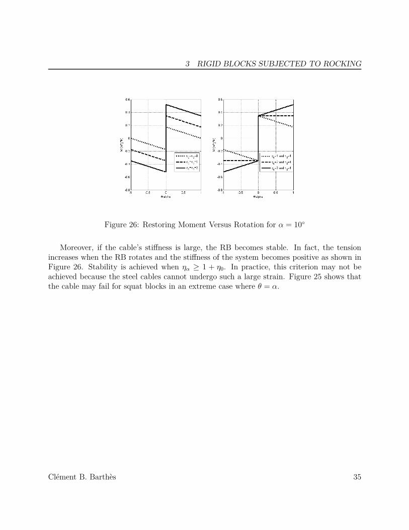
Figure 26: Restoring Moment Versus Rotation for α = 10◦
Moreover, if the cable’s stiffness is large, the RB becomes stable. In fact, the tensionincreases when the RB rotates and the stiffness of the system becomes positive as shown inFigure 26. Stability is achieved when ηα ≥ 1 + η0. In practice, this criterion may not beachieved because the steel cables cannot undergo such a large strain. Figure 25 shows thatthe cable may fail for squat blocks in an extreme case where θ = α.
Clément B. Barthès 35

3 RIGID BLOCKS SUBJECTED TO ROCKING
3.4.1 Implementation of the PT-RB Model
The dynamic behavior of a RB with a post-tension cable is examined under different typesof excitations in this section. The response is calculated by numerical integration of equa-tion (20), expressed as a 2-DOF first order ODE, using a fourth order explicit Runge-Kuttamethod (Dormand-Prince pair). The system becomes stiff when θ becomes very large (be-yond overturning angle); therefore, an implicit scheme is more efficient to detect overturning.
{y(t)
}=
{θ(t)θ(t)
}with
{f(t)
}=
{ddt
y(t)}
{f+(t)
}=
{θ(t)
−p2[sin(αθ(t)) + ug
gcos(α − θ(t))]
}for θ > 0
{f−(t)
}=
{θ(t)
−p2[sin(−αθ(t)) + ug
gcos(−α − θ(t))]
}for θ < 0
Note that not only the restoring moment but also the velocity are discontinuous for θ = 0because of Equation (3). The ODE solver has to stop when the rocking event occurs, com-putes the angular velocity after impact, and restarts with the updated initial conditions.This category of solvers was studied by Shampine and al. [31].
In the papers presented in this chapter, a conventional ODE solver is used to solve thediscontinuous equation (20). But the discontinuity occurs at the same time as the rockingevent. Therefore, it is much more efficient to solve the continuous function f+ when θ ≥ 0and f− when θ ≤ 0. Figure 27 represents the continuous functions used by the ODE solver.For instance, if the algorithm tries to converge from θ < 0 to θ = 0 but overshoots, insteadof computing the ’true’ system response, it is more effective to keep computing the continu-ous function f−(t). Once the convergence is achieved, the updated boundary conditions areapplied and the algorithm solves for f+(t). Hence the solver never encounters discontinuitieswhile it is iterating.
Clément B. Barthès 36

3 RIGID BLOCKS SUBJECTED TO ROCKING
−0.4 −0.3 −0.2 −0.1 0 0.1 0.2 0.3 0.4
−0.5
−0.4
−0.3
−0.2
−0.1
0
0.1
0.2
0.3
0.4
0.5
θ
θ
f+
f−
Discontinuous function
Figure 27: Continuous Functions f+ and f− Used By the ODE Solver
Clément B. Barthès 37

3 RIGID BLOCKS SUBJECTED TO ROCKING
Figure 28: Free Vibration Response With an Initial Rotation θ0 = α/2. RB Properties Arep = 2.0(1/sec),α = 10◦
3.4.2 Free Vibration Response
Figure 28 shows the free vibration response of a free-standing and PT-RBs. The initial ro-tation of the RB is θ0 = α/2. It is observed that the period decreases as the rotation angledecreases. The post-tension cable does not add any damping but, since the post-tensionedRB oscillates faster than the free-standing RB, the amplitude of rotation decreases faster.Otherwise, the behavior of the two RBs is very similar. Since no overturning will occur forthe given initial conditions, both RBs remain stable.
3.4.3 Response to a Ground Acceleration Pulse
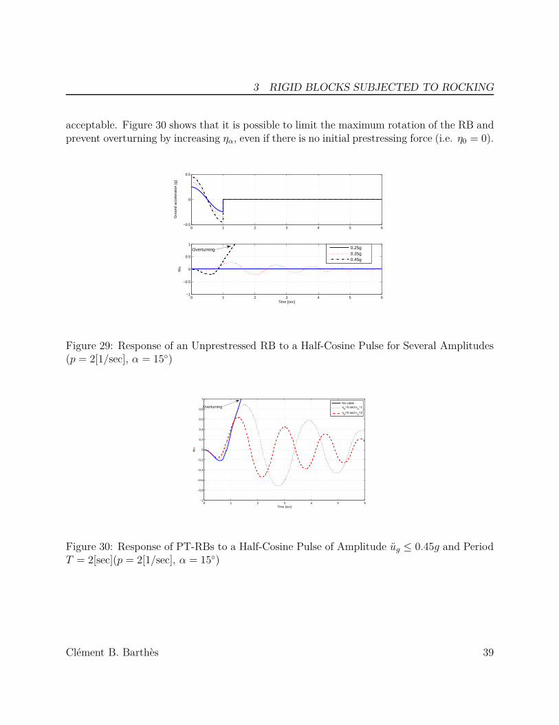
When an unprestressed RB is subjected to a constant ground acceleration sufficient to initiaterocking, it overturns. Therefore, the push-over analysis is not suitable to study the earth-quake stability of rocking structures. It was shown in this section that a prestressing cablecan stabilize a RB, but their dynamic response remain highly non-linear. It is proposed inthis section to study the behavior of a PT-RB to a half cosine ground acceleration pulse. Thistype of loading was already studied by Konstantinidis and Makris [19] for unprestressed RBs.
Figure 29 shows the response of an unprestressed RB to a ground acceleration pulse. Forug ≤ 0.25g, the RB does not rock, but for ug ≥ 0.45g the RB overturns. It was shown thatthe initial prestressing force of a PT cable allows rocking initiation to be controlled. Therocking motion should occur during a large earthquake to dissipate energy. Therefore, thecable has to be tuned to allow rocking but to limit it such that the amount of rotation is
Clément B. Barthès 38
3 RIGID BLOCKS SUBJECTED TO ROCKING
acceptable. Figure 30 shows that it is possible to limit the maximum rotation of the RB andprevent overturning by increasing ηα, even if there is no initial prestressing force (i.e. η0 = 0).
0 1 2 3 4 5 6−0.5
0
0.5G
roun
d ac
cele
ratio
n [g
]
0 1 2 3 4 5 6−1
−0.5
0
0.5
1
Time [sec]
θ/α
0.25g0.35g0.45g
Overturning
Figure 29: Response of an Unprestressed RB to a Half-Cosine Pulse for Several Amplitudes(p = 2[1/sec], α = 15◦)
0 1 2 3 4 5 6−1
−0.8
−0.6
−0.4
−0.2
0
0.2
0.4
0.6
0.8
1
Time [sec]
θ/α
No cableη
0=0 and ηα=1
η0=0 and ηα=2
Overturning
Figure 30: Response of PT-RBs to a Half-Cosine Pulse of Amplitude ug ≤ 0.45g and PeriodT = 2[sec](p = 2[1/sec], α = 15◦)
Clément B. Barthès 39

3 RIGID BLOCKS SUBJECTED TO ROCKING
3.5 Rocking SpectraAs proposed by Makris and Konstantinidis [22], it is possible to compute rocking spectra,comparable to oscillation spectra widely used nowadays. An oscillation spectrum shows themaximum acceleration of a single DOF system for a given natural frequency, a dampingratio, and an earthquake excitation. Similarly, the rocking spectra represent the maximumrotation of a rigid block for a given frequency parameter p, a slenderness angle α, and anearthquake excitation.
Rocking spectra for PT-RBs are presented in this section. Similarly to spectra computedby Makris and Konstantinidis [22], it gives the maximum rotation of a PT-RB for differentparameters. In some cases, the post-tensioning cable has an amplifying effect. For instance,in Figure 31, for α = 10◦, 2π/p = 6sec and ηα = η0 = 0.5, the PT-RB undergoes a rota-tion approximately 30% higher than the unprestressed RB. This observation still holds forηα = 5η0 and ηα = 10η0. Since the frequency of rocking will increase with the use of the PTcable, resonance may occur for some specific earthquakes. The time history acceleration ofan earthquake is very random, and since the RB response is highly non-linear, some frequen-cies may be excited when a PT cable is added. The resonance of PT-RB is usually balancedby the added stability, and for large prestressing forces (η0 ≥ 1), observations show that thecable is always beneficial.
The complex resonance phenomenon may lead to surprising results. Thus, the results ofthe rocking spectra cannot be extrapolated as easily as the results given by oscillation spectra.Two major differences must be noted. For oscillation spectra, it is possible to scale the re-sponse to simulate an earthquake excitation of a larger amplitude. Furthermore, multi-DOFelastic oscillators can be decomposed into orthogonal modes, hence the spectra can be usedto design multi-DOF structures. This is not the case with multiple blocks rocking structures.
Unlike free rocking blocks, the PT-RB can rotate beyond α and return, rather than over-turn. Since the resisting moment has a positive slope as described in Figure 16, it can intheory rotates beyond the angle α. However, the spectra presented here do not show themaximum angle when it exceeds the overturning angle of an unprestressed RB. It is consid-ered that at such large rotations, it will experience very large strains (see Figure 25).
Clément B. Barthès 40

3 RIGID BLOCKS SUBJECTED TO ROCKING
Figure 31: Rocking Spectra of PT-RBs, Subjected to Kobe Earthquake (Japan,1995, Taka-tori Station, Longitudinal), α is Equal to Respectively 5◦, 10◦, and 15◦
Clément B. Barthès 41
3 RIGID BLOCKS SUBJECTED TO ROCKING
3.6 Design Strategy Using a Rocking BaseThe rocking mechanism can be used as a dissipative system for large structures subjectedto earthquake excitation. Chen et al. [4] studied the rocking dissipation of slender viaductcolumns. In their study, the rocking mechanism is rarely used because it is hard to predictoverturning and also because it is hard to adjust the initiation of rocking. Namely, if therocking behavior is used as a seismic isolation, the structure must start to uplift before it un-dergoes major damages. It was shown that the rocking impacts dissipate energy. But, if thecolumn is slender, this dissipation will be minimal. However, when the base of the columnis uplifted, it limits the resisting moment within the column. Furthermore, the non-linearoscillations of the rocking structure, the earthquake excitation is unlikely to resonate.
The use of post-tensioned rocking system for seismic response modification for a standardordinary California bridge is presented here. The bridge section presented in Figure 32 wasfirst studied by Ketchum et al. [18].
The column is considered rigid and the girder is modeled as a lumped mass, equal to themass of the two adjacent mid-spans. The stiffness of the girder is neglected, so the bridgecolumn can be modeled as a single degree of freedom. Rocking is allowed only between thepile cap and the column and at the foot of the column. For a typical 100′ span, the rockingparameters become p = 1.1225[1/sec] and α = 4◦. Note that the lumped mass on top ofthe column increases the block slenderness (αcolumn = 7.1◦). In order to get a stable rockingcolumn, the post-tension force parameters η0 and ηα can be adjusted. Also, the foot of thecolumn may be widened in order to increase α.
In order to tune the rocking parameters properly, several design objectives have to beconsidered. The rocking mechanism is used in order to reduce the demand on the column.It helps to reduce the moment and shear in the column. In addition, the forces transferredto the footing and the deck are also lowered. Another design objective is to ensure that thebridge deformations remain acceptable. If the rocking rotations are too large, the structuremay overturn. Therefore, the rocking parameters must be chosen adequately in order tolimit the column’s demand as well as to limit the bridge deformation. Since the response ofthe structure is highly non-linear, a trial and error strategy is used.
The unprestressed column will start rocking for ug = 0.07g. Given that rocking has tooccur for ug ≥ 0.2g in order to limit the moment the foot of the column, η0 = 1.86 based onEquation (21).
The cable is first assumed to be very soft (i.e. small diameter), hence η0 = ηα. The bridge
Clément B. Barthès 42

3 RIGID BLOCKS SUBJECTED TO ROCKING
Figure 32: Typical Section of a Multi-Span Bridge
Clément B. Barthès 43

3 RIGID BLOCKS SUBJECTED TO ROCKING
is subjected to Tabas earthquake record motion (1978). Figure 34 shows the rotation of thecolumn during the excitation. η0 = 0 represents the case with no post-tensioning cable thestructure overturns almost immediately. For η0 = ηα = 1.86, the structure can withstandthe earthquake. But the rotation of the column exceeds 80% of α. Furthermore, there isalmost no dissipation. The structure is still largely oscillating 20 seconds after the end ofthe excitation.
Figure 33: Bridge Column subjected to Tabas EQ With η0 = 0 and η0 = 1.86
In order to reduce the amplitude of the rotation, the cable stiffness EAL
can be increased.Hence, a cable with a larger diameter can be used. However, it is also possible to partiallybond the cable to reduce the length allowed to elongate. As a consequence, ηα will increase.But the small dissipation comes from the slenderness of the column. Even though the footof the column could be widened to increase α, the dissipation would remain small. Otherdissipation devices can be added to slender structure such as this one.
A new run is performed with ηalpha = 10η0. Figure 35 shows that the rotation is signifi-cantly reduced. Its maximum is 24% of α.
The maximum force in the post-tension cable is FpMax = 5.9Weight. For the bridgecolumn studied here, this capacity can be obtained using a 5in2 steel cable with a yieldingstrength of 270ksi. But such cable would be too soft. In order to obtain the parameter ηα,the cable can be partially bonded as shown in Figure 33. The cable has to be unbonded overa length of about 30ft to satisfy the mechanical properties used above.
Clément B. Barthès 44

3 RIGID BLOCKS SUBJECTED TO ROCKING
Figure 34: PT-RB with a partially bonded cable
Figure 35: Bridge column subjected to Tabas EQ With η0 = 1.86 and ηα = 18.6
Clément B. Barthès 45

3 RIGID BLOCKS SUBJECTED TO ROCKING
This simplified model shows the potential benefits of rocking behaviour in large struc-tures. The moment at the base of the column will be considerably reduced, allowing thedesigners to reduce the moment capacity of the column and the footing. It also shows thatthe damping due to rocking is very small for slender structures such as bridges. Figures 34and 35 show that the oscillations are still very large, 20sec after the end of the excitation;thus, an extra damping device may be required at the base.
In conclusion, a PT-RB is an effective seismic response modification mechanism. Itsprincipal benefits are:
• Effective control of rocking initiation
• Limitation of the rocking amplitude
• Vibration period shift, making it difficult for the structure to enter resonance
This makes the structure less sensitive to earthquake excitation. But the dissipativeproperty observed on squat blocks is negligible for very slender structures. Hence rockingconnections should be coupled with external damping devices to control the attenuation ofmotion.
3.7 ConclusionA PT-RB is an effective seismic response modification mechanism. Its principal benefits are:
• Effective control of rocking initiation
• Limitation of the rocking amplitude
• Vibration period shift, making it difficult for the structure to enter resonance
This makes the structure less sensitive to earthquake excitation. But the dissipativeproperty observed on squat blocks is negligible for very slender structures. Hence rockingconnections should be coupled with external damping devices to control the attenuation ofmotion.
The equations governing a rigid block subjected to rocking are fairly simple but theycannot be represented by an oscillating system. Hence the spectral analysis widely used in
Clément B. Barthès 46

3 RIGID BLOCKS SUBJECTED TO ROCKING
earthquake engineering cannot be applied here. Makris and Konstantinidis [22] have devel-oped rocking spectra, allowing the designers to know the maximum rotation that a rigidstructure may experience for a given earthquake. However, the oscillation spectra are conve-nient because they can be used for multi DOF systems using modal analysis with a statisticalapproach. Furthermore, oscillation spectra can be blended together in order to represent thelikelihood of an earthquake event for a given region. They can be scaled since the oscillationsystems behave linearly. None of these properties applies to the rocking spectra, hence theiruse is much more limited.
The double RB assemblies were presented in section 3.3. The complexity of the im-plementation is due to the very large number of events. In fact, a single RB has a rockinginitiation defined by one equation, versus 8 equations for a double RB. A single RB in motionmay be subjected to only one impact event, versus 6 for a double RB. If a three rigid blocksassembly was to be implemented, the amount of events would be so large that it would bealmost impossible to define them all. Furthermore, such a vast amount of events would beextremely hard to solve for conventional ODE solvers because of the likelihood that severalevents happen during the same time step. Hence we can conclude that analytical rigid bodymodels are not suitable for multi-DOF rocking assemblies.
At last, the purpose of the research presented in this thesis is to study the behaviorof bridges subjected to rocking. But the rigid block assumption cannot hold for slenderstructures because the structural elements of a bridge are not rigid but deformable. Thematerial deformations may interact with the rocking rotation. Furthermore, it is likely thata bridge structure will require several rocking surfaces (between the deck and the column,for instance). These problems were an incentive to address the mechanics of rocking ina different manner. It has been already shown that the finite element method allows torepresent complex material deformations, it is proposed to design a connection elementcapable of modeling the rocking rotation. Such element could be used in combination withexisting finite elements to represent the behavior of a deformable rocking structure.
Clément B. Barthès 47

4 ROCKING ELEMENT
4 Rocking Element
4.1 IntroductionThe rocking rigid body model is very convenient to analyze the response of single degree offreedom systems. It only has a few non-dimensional parameters. However, for systems withmultiple rocking surfaces, the complexity rises tremendously. Different rocking modes mayappear; thus, the algorithm has to detect when each rocking event is triggered as explainedin [31] and it also has to detect the transition between two different rocking modes. Twosuperimposed rigid blocks lead to ten different rocking modes transitions [28], so three su-perimposed rigid blocks analysis is merely intractable. Therefore, the analytical equationsof staggered rigid blocks is not conceivable to study large structures. A finite element modelmay be more suitable.
Furthermore, a flexible block may have a significantly different rocking behavior. In or-der to use rocking devices on slender structures such as bridges, the deformations of thestructural elements must be taken into account as they may alter the rocking behavior whendeformed elastically, inducing or precluding overturning, compared to a rigid body. Thisleads to the conclusion that the rocking surface cannot be modeled independently from therest of the structure.
The goal in this chapter is to develop a finite element model representing rocking at theinterface between two prismatic (frame) finite elements. Rocking is assumed to occur in theplane of the frame (2-dimensional rocking) and the frame elements are assumed to have nothickness; i.e., the shape of the cross-sections at the rocking interface is irrelevant; only thethickness dimension of the frame element matters. The width of the rocking surface is definedas a parameter of the rocking element and it is independent of the width of the adjacentframe elements. In addition, it will allow the consideration of the large displacements anddeformations of the frame elements in the structure.
Clément B. Barthès 48
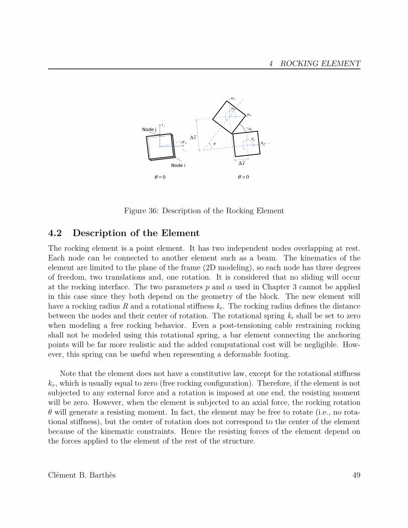
4 ROCKING ELEMENT
Figure 36: Description of the Rocking Element
4.2 Description of the ElementThe rocking element is a point element. It has two independent nodes overlapping at rest.Each node can be connected to another element such as a beam. The kinematics of theelement are limited to the plane of the frame (2D modeling), so each node has three degreesof freedom, two translations and, one rotation. It is considered that no sliding will occurat the rocking interface. The two parameters p and α used in Chapter 3 cannot be appliedin this case since they both depend on the geometry of the block. The new element willhave a rocking radius R and a rotational stiffness kr. The rocking radius defines the distancebetween the nodes and their center of rotation. The rotational spring kr shall be set to zerowhen modeling a free rocking behavior. Even a post-tensioning cable restraining rockingshall not be modeled using this rotational spring, a bar element connecting the anchoringpoints will be far more realistic and the added computational cost will be negligible. How-ever, this spring can be useful when representing a deformable footing.
Note that the element does not have a constitutive law, except for the rotational stiffnesskr, which is usually equal to zero (free rocking configuration). Therefore, if the element is notsubjected to any external force and a rotation is imposed at one end, the resisting momentwill be zero. However, when the element is subjected to an axial force, the rocking rotationθ will generate a resisting moment. In fact, the element may be free to rotate (i.e., no rota-tional stiffness), but the center of rotation does not correspond to the center of the elementbecause of the kinematic constraints. Hence the resisting forces of the element depend onthe forces applied to the element of the rest of the structure.
Clément B. Barthès 49

4 ROCKING ELEMENT
The displacements and the rotations of the nodes expressed in the global coordinate sys-tem are stored in the vector u. The forces and the moments at the nodes are stored in thevector p. The two nodes can translate and rotate separately but, in order to model rockingwithout sliding, these translations and rotations are dependent. Hence only one internaldegree of freedom, the angle, remains.
The element has an orientation, so there is an initial angle θ0 that defines the anglebetween the rocking surface and the ex-axis as shown in Figure 36. When rocking occurs,the kinematic equations are the following:
Δx = −sign (θ) R (1 − cos θ) (22a)Δy = R| sin θ| (22b)
−1
−0.5
0
0.5
1
θ
Δx
R
−π/2 −π/4 0 π/4 π/2
0
0.2
0.4
0.6
0.8
1
θ
Δy
R
−π/2 −π/4 0 π/4 π/2
Figure 37: Kinematics of the Rocking Element
The kinematic constraints are imposed using the Lagrange multiplier method. Beforerocking occurs, the two nodes must overlap. Therefore, the algorithm applies the followingthree constraints.
Clément B. Barthès 50

4 ROCKING ELEMENT
g1(u) = u4 − u1 = 0 (23a)g2(u) = u5 − u2 = 0 (23b)g3(u) = u6 − u3 = 0 (23c)
Once rocking is initiated, then the three constraint functions defined in Equations (23a),(23b), and (23c) are replaced by the two constraint functions (24a) and (24b). These twoconstraints impose the vertical and horizontal displacements consistent with the radius Rfor a rotation θ. The center of rotation is located at a distance R from the nodes. The initialangle θ0 defines the initial orientation of the rocking surface. These constraints also preventsliding. The relative displacements between the nodes are represented in Figure 37. Notethat the horizontal displacement is smooth; however, the vertical displacement has no firstderivative for θ = 0.
g1(u) = (u4 − u1) cos(u3 + θ0) + (u5 − u2) sin(u3 + θ0) + sign(u6 − u3)R(1 − cos(u6 − u3))(24a)
g2(u) = −(u4 − u1) sin(u3 + θ0) + (u5 − u2) cos(u3 + θ0) − R| sin(u6 − u3)| (24b)
4.3 Initiation of RockingA block uplifts when one end of its rocking base is no longer subjected to compression sothe element will initiate rocking when the axial compression multiplied by the radius of thebase is less than the moment applied at the node . It is important to note that the elementcan be subjected to a rigid body motion; so, in general, the direction of the axial force is notaligned with the vertical axis.
In equation (25) the forces and moments pi are associated with the displacements androtations ui and the internal rotation θ is equal to zero since rocking has not occured. Whenrocking is initiated, the constraints are changed. The three constraint functions (23) arereplaced by the two constraint functions (24). A Lagrange multiplier will disappear, so thestructure of the global stiffness matrix will change. This event has to be handled with greatcare by the algorithm. It corresponds to a sudden change in the boundary conditions ofthe structure, hence the transition should occur when the system respect the constraints
Clément B. Barthès 51

4 ROCKING ELEMENT
associated with the non-rocking state (23) and the constraints associated with the rockingstate (24). This transition should occur when the rocking initiation event is satisfied andwhen the internal rotation in the rocking element is θ = 0.
p3 > −R(− sin(u3 + θ0) cos(u3 + θ0)
)(p4 − p1p5 − p2
)(25)
If the algorithm overshoots when the rocking is initiated, the moment in the element willfar exceed the moment defined by equation (25). The release of a constraint will then lead toa sudden drop of the moment and generate noise while, in fact, the resisting moment shouldbe continuous when rocking is initiated. Therefore, when the event occurs, the algorithm hasto step back and reduce the time step in order to converge to the rocking initiation event.This issue was discussed in chapter 3.4.1, for the rocking event detection (at each impact)and not for the rocking initiation event.
As a structure undergoes free rocking, the amplitude is reduced and the oscillationsbecome shorter after each impact. Eventually, the rocking rotations are too small and thealgorithm should interrupt rocking to minimize computational cost.
Clément B. Barthès 52

4 ROCKING ELEMENT
4.4 Implementation of the ConstraintsIn order to represent the rocking motion properly, the rest of the structure has to be mod-eled with elements accounting for large displacements. The location of the center of masseswith respect to the center of rotation of rocking will play a central role in the rocking be-havior and in the loss of stability of the structure. The beam elements used in this thesisare elastic corotational beam elements [6], embedded in FEDEASLab [11]. This programallows the user to call any existing routine in Matlab as well as a robust linear algebra solver.
The rocking elements are associated with constraints. Therefore, an energy potential forthe entire structure (rocking and elastic elements) has to be minimized and to satisfy theconstraint functions gi(u), using the Lagrange multiplier method.
Πtot(u, λ) = Π(u) + λg(u) (26)
=⇒⎧⎨⎩
∂Πtot
∂u = R(u) + ( ∂g∂u)Tλ − F
∂Πtot
∂λ= g(u)
(27)
Equations (26) and (27) describe the governing equations of the structure with the con-straints. u represents the displacements at the free degrees of freedom (DOF) , R(u) rep-resents the resisting force associated with the free DOFs, F represents the applied force,including the inertia forces, and g(u) represents the constraint functions associated with thefree DOFs connected to a rocking element.
Since these equations are non-linear, this potential will be minimized using an incremen-tal and iterative algorithm. Equation (28) shows that the total stiffness matrix is symmetricbut not positive definite. Hence the Cholesky solving algorithm cannot work because thepivots are equal to the diagonal terms and cannot be zero. The matrix can still be invertedwith a permutation algorithm, but the computational cost increases. In such cases, it isusually preferred to enforce the constraints with approximate methods [17].
K = ∂R
∂u, L = ∂g
∂u=⇒
[K LT
L 0
](ΔuΔλ
)=
(ΔFΔg
)(28)
The penalty method consists of multiplying the constraint functions by a very largepenalty number such that, when the potential is minimized ,the constraint function has toremain small.
Πκ(u) = Π(u) + 12
κg(u)2 with κ � 1 (29)
Clément B. Barthès 53
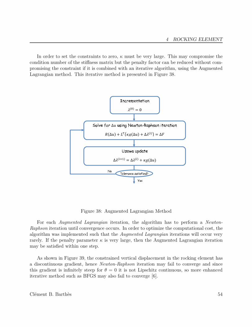
4 ROCKING ELEMENT
In order to set the constraints to zero, κ must be very large. This may compromise thecondition number of the stiffness matrix but the penalty factor can be reduced without com-promising the constraint if it is combined with an iterative algorithm, using the AugmentedLagrangian method. This iterative method is presented in Figure 38.
Figure 38: Augmented Lagrangian Method
For each Augmented Lagrangian iteration, the algorithm has to perform a Newton-Raphson iteration until convergence occurs. In order to optimize the computational cost, thealgorithm was implemented such that the Augmented Lagrangian iterations will occur veryrarely. If the penalty parameter κ is very large, then the Augmented Lagrangian iterationmay be satisfied within one step.
As shown in Figure 39, the constrained vertical displacement in the rocking element hasa discontinuous gradient, hence Newton-Raphson iteration may fail to converge and sincethis gradient is infinitely steep for θ = 0 it is not Lipschitz continuous, so more enhancediterative method such as BFGS may also fail to converge [6].
Clément B. Barthès 54

4 ROCKING ELEMENT
0
0.2
0.4
0.6
0.8
1
θ
Δy
R
−π/2 −π/4 0 π/4 π/2
−1
−0.5
0
0.5
1
θ
∂
∂θ
(Δy
R
)
−π/2 −π/4 0 π/4 π/2
Figure 39: Vertical Constraint of the Rocking Element Versus Rotation
Therefore, a different approach was used. Instead of trying to find an algorithm thatconverges, despite the discontinuity, the vertical constraint function was ’smoothed.’ Whenθ is within an interval ε near zero, Equation (22b) is interpolated with an order 4 poly-nomial. Hence its derivative is continuous at zero. This method makes the element morerobust because it allows the user to use any iterative algorithm, suitable for the rest of thestructure. In order to enforce the continuity at the edge of the interval ε , the function ismade so that it is no longer equal to zero for θ = 0. In Figure 40, a very large interval ε waschosen for clarity. Equation (31) represents the smoothed constraint functions used when|θ| < ε, with the polynomial coefficients expressed in Equation (30)
⎛⎜⎝
a1a2a3
⎞⎟⎠ =
⎛⎜⎝
− 18ε2 sin(ε) − 1
8ε3 cos(ε)−1
2 sin(ε) − 6αε2
sin(ε) − αε4 − βε2
⎞⎟⎠ (30)
g1ε = (u4 − u1) cos(u3 + θ0) + (u5 − u2) sin(u3 + θ0) + sign(u6 − u3)R(1 − cos(u6 − u3))(31a)
g2ε = −(u4 − u1) sin(u3 + θ0) + (u5 − u2) cos(u3 + θ0) − R(a1(u6 − u3)4 + a2(u6 − u3)2 + a3)(31b)
Inevitably, the ’softening’ parameter ε will reduce the intensity of the impact, so it willaffect restitution. Figure 42 represents the rotation of a rocking element for a column sub-jected to free rocking behavior. The initial angle of the column is equal to its slendernessangle (i.e. θini = α). It shows that for ε ≥ θini, the rocking element does not dissipate any
Clément B. Barthès 55
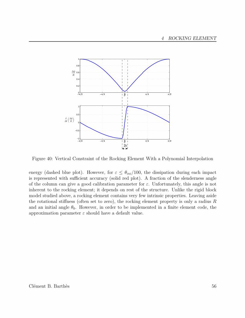
4 ROCKING ELEMENT
0
0.2
0.4
0.6
0.8
1
θ
Δy
R
−π/2 −π/4 0 π/4 π/2−π/2 −π/4 0 π/4 π/2
−1
−0.5
0
0.5
1
θ
∂
∂θ
(Δy
R
)
−π/2 −π/4 0 π/4 π/2−π/2 −π/4 0 π/4 π/2
2ε
Figure 40: Vertical Constraint of the Rocking Element With a Polynomial Interpolation
energy (dashed blue plot). However, for ε ≤ θini/100, the dissipation during each impactis represented with sufficient accuracy (solid red plot). A fraction of the slenderness angleof the column can give a good calibration parameter for ε. Unfortunately, this angle is notinherent to the rocking element; it depends on rest of the structure. Unlike the rigid blockmodel studied above, a rocking element contains very few intrinsic properties. Leaving asidethe rotational stiffness (often set to zero), the rocking element property is only a radius Rand an initial angle θ0. However, in order to be implemented in a finite element code, theapproximation parameter ε should have a default value.
Clément B. Barthès 56
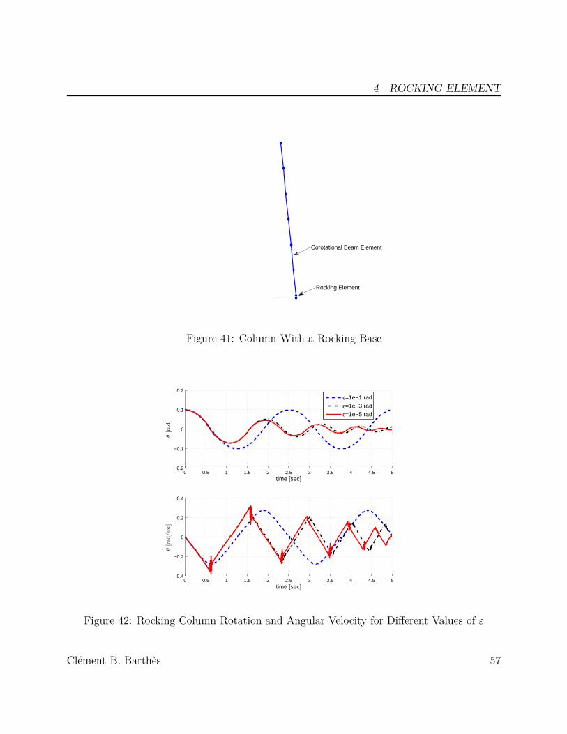
4 ROCKING ELEMENT
Corotational Beam Element
Rocking Element
Figure 41: Column With a Rocking Base
0 0.5 1 1.5 2 2.5 3 3.5 4 4.5 5−0.2
−0.1
0
0.1
0.2
time [sec]
θ[rad
]
0 0.5 1 1.5 2 2.5 3 3.5 4 4.5 5−0.4
−0.2
0
0.2
0.4
time [sec]
θ[rad
/sec
]
ε=1e−1 radε=1e−3 radε=1e−5 rad
Figure 42: Rocking Column Rotation and Angular Velocity for Different Values of ε
Clément B. Barthès 57
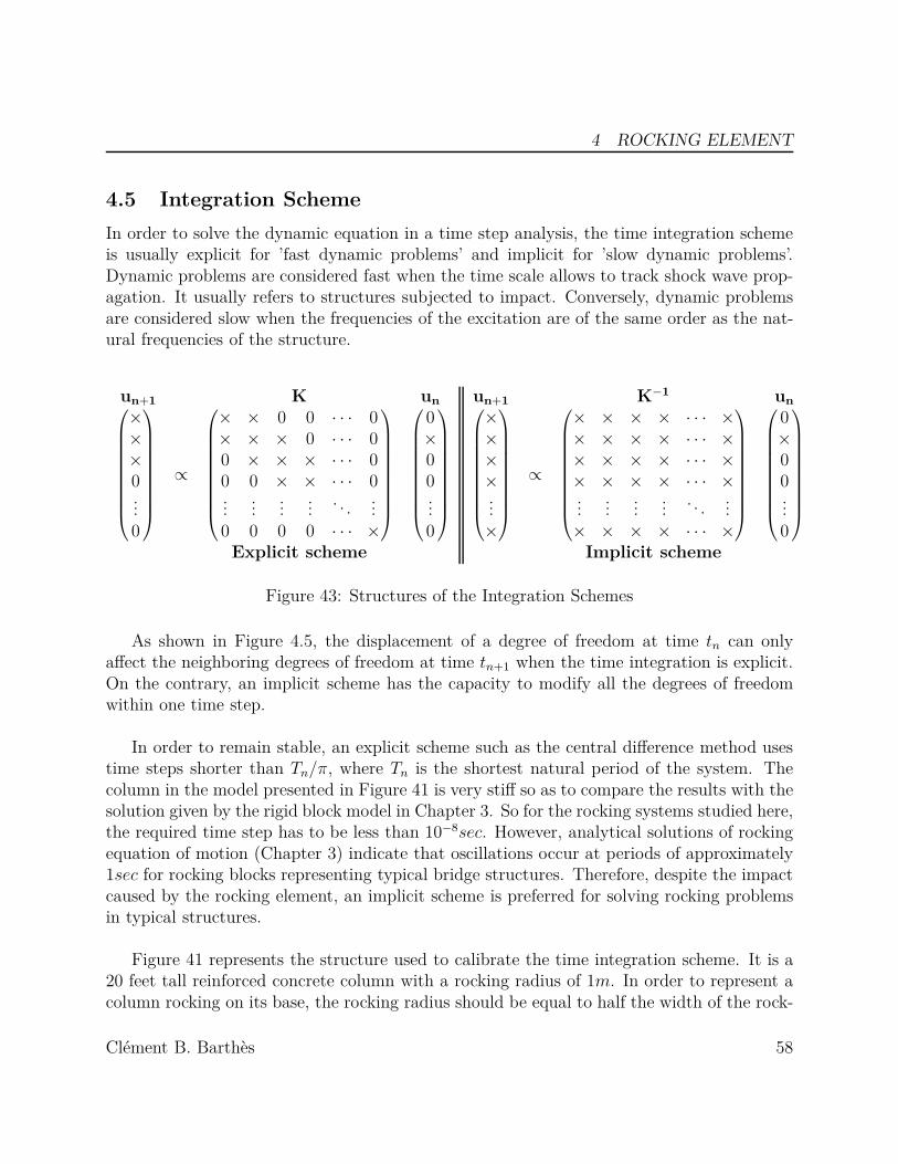
4 ROCKING ELEMENT
4.5 Integration SchemeIn order to solve the dynamic equation in a time step analysis, the time integration schemeis usually explicit for ’fast dynamic problems’ and implicit for ’slow dynamic problems’.Dynamic problems are considered fast when the time scale allows to track shock wave prop-agation. It usually refers to structures subjected to impact. Conversely, dynamic problemsare considered slow when the frequencies of the excitation are of the same order as the nat-ural frequencies of the structure.
un+1 K un un+1 K−1 un⎛⎜⎜⎜⎜⎜⎜⎜⎜⎜⎝
×××0...0
⎞⎟⎟⎟⎟⎟⎟⎟⎟⎟⎠
∝
⎛⎜⎜⎜⎜⎜⎜⎜⎜⎜⎝
× × 0 0 · · · 0× × × 0 · · · 00 × × × · · · 00 0 × × · · · 0... ... ... ... . . . ...0 0 0 0 · · · ×
⎞⎟⎟⎟⎟⎟⎟⎟⎟⎟⎠
⎛⎜⎜⎜⎜⎜⎜⎜⎜⎜⎝
0×00...0
⎞⎟⎟⎟⎟⎟⎟⎟⎟⎟⎠
⎛⎜⎜⎜⎜⎜⎜⎜⎜⎜⎝
××××...×
⎞⎟⎟⎟⎟⎟⎟⎟⎟⎟⎠
∝
⎛⎜⎜⎜⎜⎜⎜⎜⎜⎜⎝
× × × × · · · ×× × × × · · · ×× × × × · · · ×× × × × · · · ×... ... ... ... . . . ...× × × × · · · ×
⎞⎟⎟⎟⎟⎟⎟⎟⎟⎟⎠
⎛⎜⎜⎜⎜⎜⎜⎜⎜⎜⎝
0×00...0
⎞⎟⎟⎟⎟⎟⎟⎟⎟⎟⎠
Explicit scheme Implicit scheme
Figure 43: Structures of the Integration Schemes
As shown in Figure 4.5, the displacement of a degree of freedom at time tn can onlyaffect the neighboring degrees of freedom at time tn+1 when the time integration is explicit.On the contrary, an implicit scheme has the capacity to modify all the degrees of freedomwithin one time step.
In order to remain stable, an explicit scheme such as the central difference method usestime steps shorter than Tn/π, where Tn is the shortest natural period of the system. Thecolumn in the model presented in Figure 41 is very stiff so as to compare the results with thesolution given by the rigid block model in Chapter 3. So for the rocking systems studied here,the required time step has to be less than 10−8sec. However, analytical solutions of rockingequation of motion (Chapter 3) indicate that oscillations occur at periods of approximately1sec for rocking blocks representing typical bridge structures. Therefore, despite the impactcaused by the rocking element, an implicit scheme is preferred for solving rocking problemsin typical structures.
Figure 41 represents the structure used to calibrate the time integration scheme. It is a20 feet tall reinforced concrete column with a rocking radius of 1m. In order to represent acolumn rocking on its base, the rocking radius should be equal to half the width of the rock-
Clément B. Barthès 58

4 ROCKING ELEMENT
ing column (i.e. R = b/2). The geometric and material parameters are chosen to representa realistic bridge column with a hollow section. An initial rotation of 0.1rad is applied tothe column and the free oscillation response is computed using a Newmark implicit scheme(β = 1/4 and γ = 1/2). The initial time step is 1e − 2sec, but the integration algorithm isable to perform time-step division when the Newton-Raphson iterations fail to converge.
Figure 44 represents the rotation and the angular velocity response of the rocking elementfor the initial conditions shown in Figure 41. Based on the results presented in Chapter 3, thecolumn is expected to rock freely and to radiate the energy released during impact throughthe column. Hence, the rotation at the base should only decrease; however,the solid blue plotin Figure 44 shows that the rotation being amplified, which leads to the instability of thestructure. It is due to the numerical noise of the angular velocity θ. After each impact, thenoise worsens. The velocity at the first impact should be the upper bound but, after a fewimpacts, the noise generated exceeds this limit in amplitude. This numerical noise is oftenobserved in structures subjected to impact [14]. High frequency noise in the displacementresponse can easily be solved by adding viscous damping but, in this case, the high frequencynoise is in the velocity response . The Newmark scheme used here is energy conservative;therefore, only a different integration scheme with a numerical dissipation can solve this issue.
The HHT method [14], also known as the α-method, is a modified Newmark scheme.Equation (32) represents the implementation with the Augmented Lagrangian contribution.The added parameter α controls high-frequency damping. It can then be used to filter outthe high frequency noise observed in the angular velocity.
Mun+1 + Cun+1 + (1 + α)(R(un+1) + λn+1∂g
∂u(un+1)) − α(R(un) + λn
∂g
∂u(un)) = Fn+1
(32a)un+1 = un + Δtun + Δt2((1/2 − β)un + βun+1)
(32b)un+1 = un + Δt((1 − γ)un + γun+1)
(32c)
The spectral radius defines the change of the displacement norm between steps n and n+1,so ρ = ||un+1||
||un|| . It is computed using the response of a linear system Mun+1+Cun+1+Kun+1 =Fn+1. If the spectral radius ρ = 1, then the integration scheme does not dissipate energy. Ifρ > 1, the scheme is unstable. Figure 45 represents the spectral radius of the HHT integra-tion scheme versus the time-steps/natural-period ratio. It shows that the Newmark method
Clément B. Barthès 59

4 ROCKING ELEMENT
0 0.5 1 1.5 2 2.5 3 3.5 4 4.5 5−0.2
−0.15
−0.1
−0.05
0
0.05
0.1
0.15
0.2
time [sec]
θ[rad
]
0 0.5 1 1.5 2 2.5 3 3.5 4 4.5 5−1.5
−1
−0.5
0
0.5
1
1.5
time [sec]
θ[rad
/sec
]
Newmark method (β=1/4, γ=1/2)HHT method (α=−1/3, β=1/4, γ=1/2)
Figure 44: Rocking Element Response to a Free Oscillation (Newmark Scheme β = 1/4 andγ = 1/2)
is not dissipative for β = 1/4 and γ = 1/2. Since the solution is not exact, the conservationof energy leads to numerical noise generation. It is observed that this noise occur in thehigh frequency range and should be filtered. The spectral radius for the HHT method isequal to 1 for low frequencies (i.e. Δt
T<< 1), but it filters the high frequencies. Hence it
is very suitable to solve the issue presented in Figure 44. The dashed plot shows that theHHT integration scheme represents a reasonable solution without the noise observed in theangular velocity.
The implementation of the HHT integration algorithm is summarized in Figure 46.
Clément B. Barthès 60

4 ROCKING ELEMENT
10−2
10−1
100
101
102
103
0
0.2
0.4
0.6
0.8
1
Δt/T
ρ
Newmark method (β=1/4, γ=1/2)
HHT method (α=−1/3, β=1/4, γ=1/2)
Figure 45: Spectral Radius of the HHT Integration Method
Clément B. Barthès 61

4 ROCKING ELEMENT
Figure 46: Summary of the HHT Algorithm Implementation
Clément B. Barthès 62
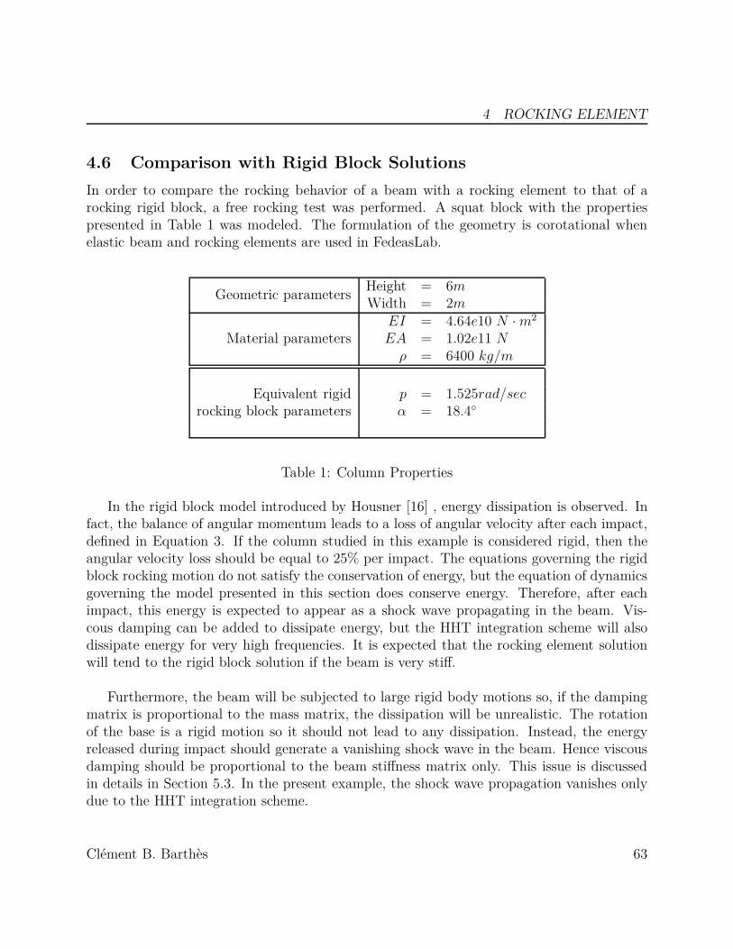
4 ROCKING ELEMENT
4.6 Comparison with Rigid Block SolutionsIn order to compare the rocking behavior of a beam with a rocking element to that of arocking rigid block, a free rocking test was performed. A squat block with the propertiespresented in Table 1 was modeled. The formulation of the geometry is corotational whenelastic beam and rocking elements are used in FedeasLab.
Geometric parameters Height = 6mWidth = 2m
Material parametersEI = 4.64e10 N · m2
EA = 1.02e11 Nρ = 6400 kg/m
Equivalent rigid p = 1.525rad/secrocking block parameters α = 18.4◦
Table 1: Column Properties
In the rigid block model introduced by Housner [16] , energy dissipation is observed. Infact, the balance of angular momentum leads to a loss of angular velocity after each impact,defined in Equation 3. If the column studied in this example is considered rigid, then theangular velocity loss should be equal to 25% per impact. The equations governing the rigidblock rocking motion do not satisfy the conservation of energy, but the equation of dynamicsgoverning the model presented in this section does conserve energy. Therefore, after eachimpact, this energy is expected to appear as a shock wave propagating in the beam. Vis-cous damping can be added to dissipate energy, but the HHT integration scheme will alsodissipate energy for very high frequencies. It is expected that the rocking element solutionwill tend to the rigid block solution if the beam is very stiff.
Furthermore, the beam will be subjected to large rigid body motions so, if the dampingmatrix is proportional to the mass matrix, the dissipation will be unrealistic. The rotationof the base is a rigid motion so it should not lead to any dissipation. Instead, the energyreleased during impact should generate a vanishing shock wave in the beam. Hence viscousdamping should be proportional to the beam stiffness matrix only. This issue is discussedin details in Section 5.3. In the present example, the shock wave propagation vanishes onlydue to the HHT integration scheme.
Clément B. Barthès 63
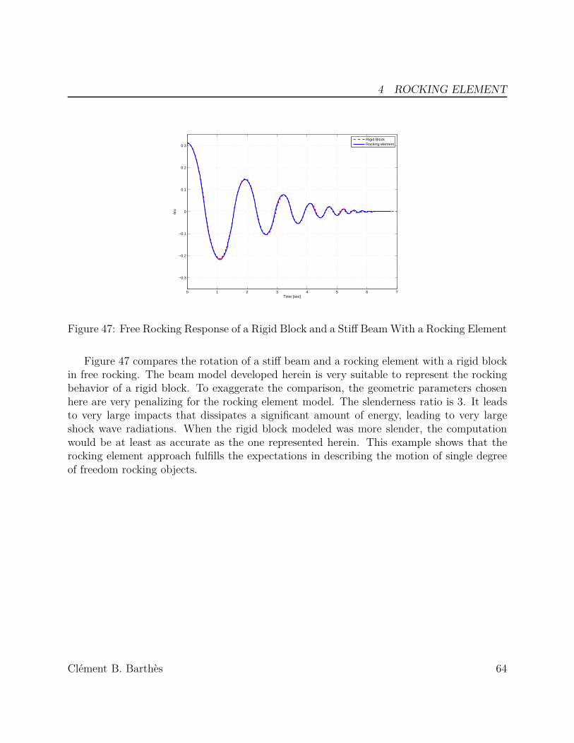
4 ROCKING ELEMENT
0 1 2 3 4 5 6 7
−0.3
−0.2
−0.1
0
0.1
0.2
0.3
Time [sec]
θ/α
Rigid BlockRocking element
Figure 47: Free Rocking Response of a Rigid Block and a Stiff Beam With a Rocking Element
Figure 47 compares the rotation of a stiff beam and a rocking element with a rigid blockin free rocking. The beam model developed herein is very suitable to represent the rockingbehavior of a rigid block. To exaggerate the comparison, the geometric parameters chosenhere are very penalizing for the rocking element model. The slenderness ratio is 3. It leadsto very large impacts that dissipates a significant amount of energy, leading to very largeshock wave radiations. When the rigid block modeled was more slender, the computationwould be at least as accurate as the one represented herein. This example shows that therocking element approach fulfills the expectations in describing the motion of single degreeof freedom rocking objects.
Clément B. Barthès 64

4 ROCKING ELEMENT
4.7 Rocking TerminationIt was shown in Section 3.1.3 that even though the number of rocking impacts is infinite,the free rocking response will stop at a finite time but, due to the ’softening’ parameter εdescribed in Section 4.4, the rocking element will act as a very stiff rotational spring whenθ 0 and the rotation will continue indefinitely with a very small amplitude.
There are two options to handle termination of rocking motion:
• The rocking rotation can be locked under a certain value
• The element can be allowed to rock even for very small rotations
A criterion, intrinsic to the element, must be chosen to stop the rocking but a rockingrotation is considered to be small when compared to the rest of the structure. Here, theoption to do nothing about stopping the small magnitude rocking motions is examined. Arigid block is excited in free rocking, followed by a ground acceleration pulse equal to 75% ofthe required ground acceleration to initiate rocking. Figure 48 shows that, once the rockingmotion vanishes, the system behaves like a column at rest. Despite this large excitation, theblock does not rock; its rotation does not increase. This is consistent since the structure canbe considered at rest. Therefore, small magnitude rocking can be allowed to remain in themodel without affecting the solution. However, as the rocking rotations become smaller, thefrequency of impacts increase. Hence the time steps shorten and the computational time ofmonitoring just minor motions becomes extremely large.
The properties of the rocking elements are not sufficient to be determined when the tipdisplacement of the column or some controlling point of the structure becomes negligible.An ’autonomous’ strategy should be preferred to simplify the use of this element. In orderto avoid an ill-conditioned stiffness matrix, the user should use units such that the stiffnessmatrix and the mass matrix of each element remain close to one. If the HHT integrationscheme is used, then the condition number of the matrix Keff = Kt + 1
Δt2 · 1β(1+α)M should
be considered. It can be assumed that if rocking rotations are less than 1e − 10rad androcking velocities are less than 1e − 7rad/[time − unit], the rocking motion is negligible androcking will be terminated. These two parameters are very severe, but they guarantee thestability of the algorithm even when the matrix Keff is poorly conditioned.
Clément B. Barthès 65

4 ROCKING ELEMENT
0 2 4 6 8 10 12 14−0.2
−0.1
0
0.1
0.2
θ[rad
]
0 2 4 6 8 10 12 14−0.5
−0.25
0
0.25
0.5
θ[rad
/sec
]
0 2 4 6 8 10 12 14−0.5
−0.25
0
0.25
0.5
time [sec]
ug g
Figure 48: Free Rocking Response, Then Subjected to a Large Ground Acceleration
Clément B. Barthès 66

4 ROCKING ELEMENT
4.8 Behavior of a Two-block AssemblyAs explained in section 3.3 the governing equations of two rigid blocks stacked were derivedin [28]. This model is much more complex than the single rigid block model. The equationsfor three or more rigid blocks would be even more difficult to derive. Such configuration isvery sensitive to small geometric variations. This can quickly lead to an overturning of thestructure, due to the inherent instability of the assembly. A two-block structure is modeledhere in order to compare the results of simulation, using the rocking element to the analyticsolution for rigid blocks presented by Psycharis, even though such configuration could hardlybe used in earthquake engineering.
0 0.5 1 1.5 2 2.5 3 3.5 4 4.5 5−0.15
−0.10
−0.05
0
0.05
0.1
0.15
Time [sec]
θ top [r
ad]
0 0.5 1 1.5 2 2.5 3 3.5 4 4.5 5−0.15
−0.1
−0.05
0
0.05
0.1
0.15
Time [sec]
θ botto
m [r
ad]
Rigid Blocks
Rocking elements
Figure 49: Free Rocking Response of a Two Rigid Blocks Assembly and a Two BeamsAssembly With Rocking Elements at Interfaces
Figure 49 compares the response of a two rigid bodies assembly with the beam and rockingelements assembly subjected to an initial rotation. The geometric parameters are presentedin Table 2; they are similar to the ones used in [28]. The rocking elements successfullyrepresent the two-block assembly behavior. The error is more noticeable than that observedin Figure 47. However, it can be explained by the high sensitivity of the model. Thesolution varies noticeably when a slight change is made to the mass distribution (lumped
Clément B. Barthès 67
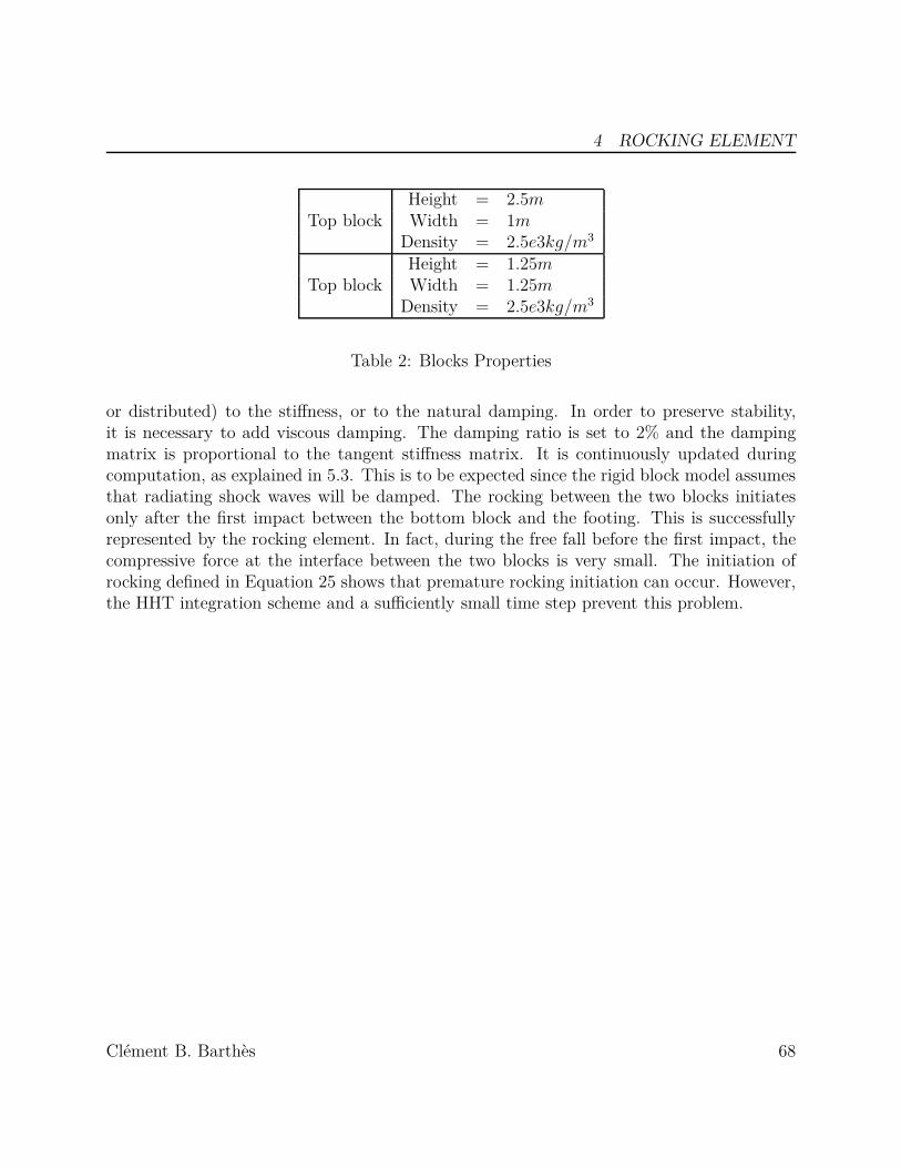
4 ROCKING ELEMENT
Top blockHeight = 2.5mWidth = 1m
Density = 2.5e3kg/m3
Top blockHeight = 1.25mWidth = 1.25m
Density = 2.5e3kg/m3
Table 2: Blocks Properties
or distributed) to the stiffness, or to the natural damping. In order to preserve stability,it is necessary to add viscous damping. The damping ratio is set to 2% and the dampingmatrix is proportional to the tangent stiffness matrix. It is continuously updated duringcomputation, as explained in 5.3. This is to be expected since the rigid block model assumesthat radiating shock waves will be damped. The rocking between the two blocks initiatesonly after the first impact between the bottom block and the footing. This is successfullyrepresented by the rocking element. In fact, during the free fall before the first impact, thecompressive force at the interface between the two blocks is very small. The initiation ofrocking defined in Equation 25 shows that premature rocking initiation can occur. However,the HHT integration scheme and a sufficiently small time step prevent this problem.
Clément B. Barthès 68

4 ROCKING ELEMENT
4.9 ConclusionIn this chapter, the implementation of a rocking element was presented. It consists of a zero-length two nodes element capable of representing the behavior of a rocking surface betweenprismatic elements. The kinematics of this element are limited to the plane of the frame.The rocking parameters presented in Chapter 3 are no longer suitable for this modeling ap-proach. Therefore, new parameters intrinsic to the element, namely, the rocking radius Rand its orientation θ0, were introduced.
This element behavior is not governed by a material constitutive law but by kinematicconstraints. The element has one degree of freedom, namely, the relative rotation betweenthe two nodes but, the center of rotation is not located at the nodes. The kinematic con-straints force the rotation to occur around a center located at a distance R from the nodes.So, when this element is used in a model, the solution cannot be obtained with a conven-tional energy minimization method. Instead, the energy minimization must also respect thekinematic constraints. An approximated solution called the Augmented Lagrangian methodwas implemented.
Several computational issues had to be addressed during the implementation of the solv-ing algorithm. First, the element can cause rocking to initiate and to terminate. By doingso, the number of constraints change during the computation. Furthermore, one of the kine-matic constraints is not Lipschitz continuous and may prevent the Newton-Raphson iterationmethod to converge. At last, the rocking impacts may cause noise in the velocity responsethat must be filtered by the integration scheme.
A stiff column was modeled with a rocking element at its base and the rocking responsewas compared with the response of a rigid body. The solution obtained was very consistent.The rocking response of two stacked rigid blocks was also approximated with success byusing stiff frame elements and rocking elements at their interface.
Thus, this element can be used to model the effect of rocking on deformable structures. Itis extensively used in the rest of this thesis address several issues concerning bridge columnssubjected to earthquake and has helped overcoming the severe limitations of the rigid blockmodel presented in Chapter 3. For instance, the fiber elements capable of representing beamswith inelastic material behavior can be used to compute the earthquake response of a slenderreinforced concrete structure allowed to rock.
Clément B. Barthès 69
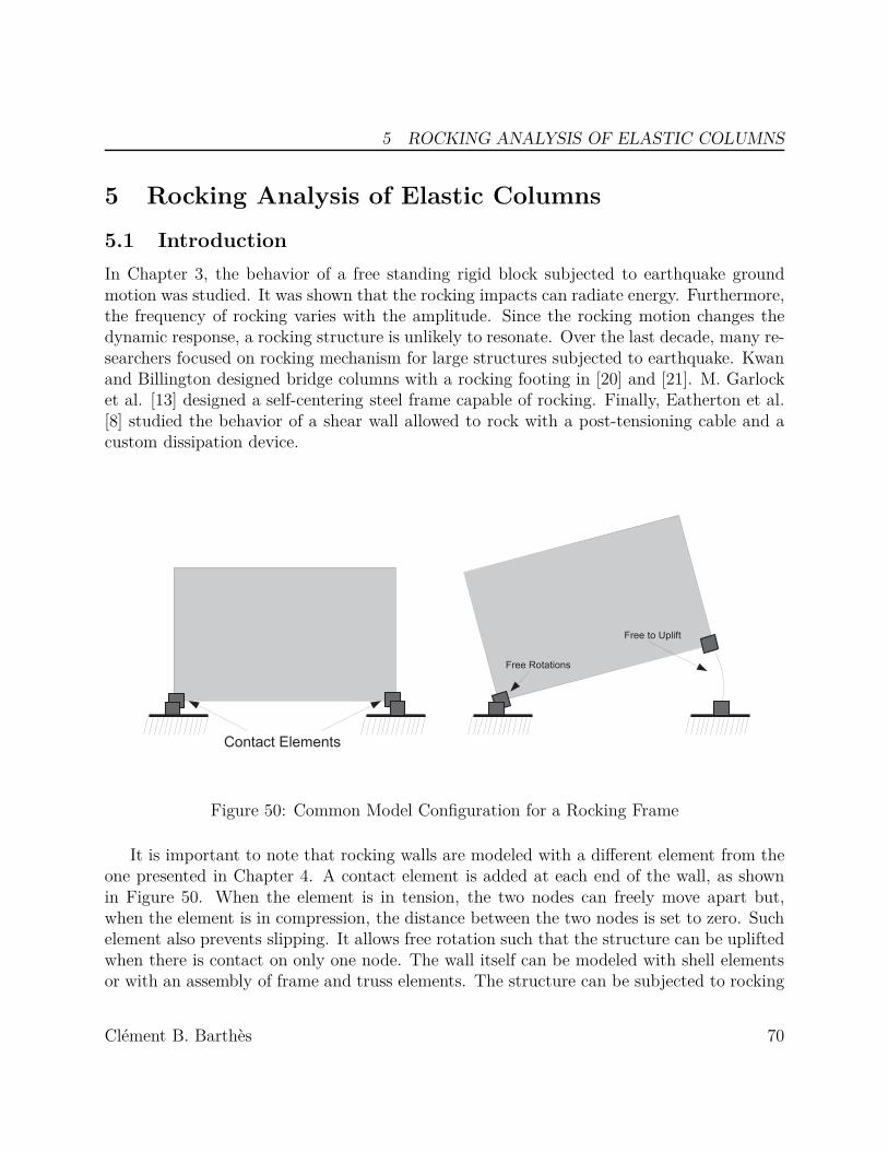
5 ROCKING ANALYSIS OF ELASTIC COLUMNS
5 Rocking Analysis of Elastic Columns
5.1 IntroductionIn Chapter 3, the behavior of a free standing rigid block subjected to earthquake groundmotion was studied. It was shown that the rocking impacts can radiate energy. Furthermore,the frequency of rocking varies with the amplitude. Since the rocking motion changes thedynamic response, a rocking structure is unlikely to resonate. Over the last decade, many re-searchers focused on rocking mechanism for large structures subjected to earthquake. Kwanand Billington designed bridge columns with a rocking footing in [20] and [21]. M. Garlocket al. [13] designed a self-centering steel frame capable of rocking. Finally, Eatherton et al.[8] studied the behavior of a shear wall allowed to rock with a post-tensioning cable and acustom dissipation device.
Figure 50: Common Model Configuration for a Rocking Frame
It is important to note that rocking walls are modeled with a different element from theone presented in Chapter 4. A contact element is added at each end of the wall, as shownin Figure 50. When the element is in tension, the two nodes can freely move apart but,when the element is in compression, the distance between the two nodes is set to zero. Suchelement also prevents slipping. It allows free rotation such that the structure can be upliftedwhen there is contact on only one node. The wall itself can be modeled with shell elementsor with an assembly of frame and truss elements. The structure can be subjected to rocking
Clément B. Barthès 70

5 ROCKING ANALYSIS OF ELASTIC COLUMNS
only if at least two nodes of the frame are connected to the footing with this contact element.But for slender structures such as bridges, the columns are modeled with frame elements.Therefore, the column and the footing are bonded with only one node, preventing the use ofcontact elements described above. This is when the rocking element presented in Chapter 4can be used.
W
E,A,I,
2R
Figure 51: Elastic Column With a Lumped Mass and a Rocking Base
5.2 Rocking-Bending InteractionFigure 51 represents a deformable column with a distributed mass and a lumped mass at thetop. The base of the column is allowed to rock. The column consists of a 400mmx400mmsquare steel tube with 12mm wall. The structure properties are presented in Table 3. In thisChapter, the Young’s Modulus Es is scaled extensively in order to emphasize the influenceof column stiffness on the structure response.
The structure was chosen such that, even without rocking, very large inertia forces areexpected. The first mode of the structure has a natural period of Tn = 0.315sec. Figure52 represents the Pseudo-Acceleration Response Spectrum of the considered earthquake. Itshows that the acceleration of the mass (that is lumped at the top of the column) would belarge for a SDOF system, responding with column oscillatory bending.
Clément B. Barthès 71

5 ROCKING ANALYSIS OF ELASTIC COLUMNS
ColumnHeight h = 6m
Young’s Modulus Es = 200GP aCross Section Area A = 18, 624mm2
Cross Section Inertia I = 4.677e8mm4
Linear Density ρ = 96.7kg/mLumped mass Mass = 3000kg
Footing Rocking Radius = 1m
Table 3: Model properties
10−2
10−1
100
101
10−2
10−1
100
101
Period [sec]
Spe
ctra
l Acc
eler
atio
n [g
]
Tn=0.315
Figure 52: Unscaled Pseudo-Acceleration Response Specrum With 2% Damping - KobeEQ(1995) - Takatori Record - Longitudinal
Clément B. Barthès 72
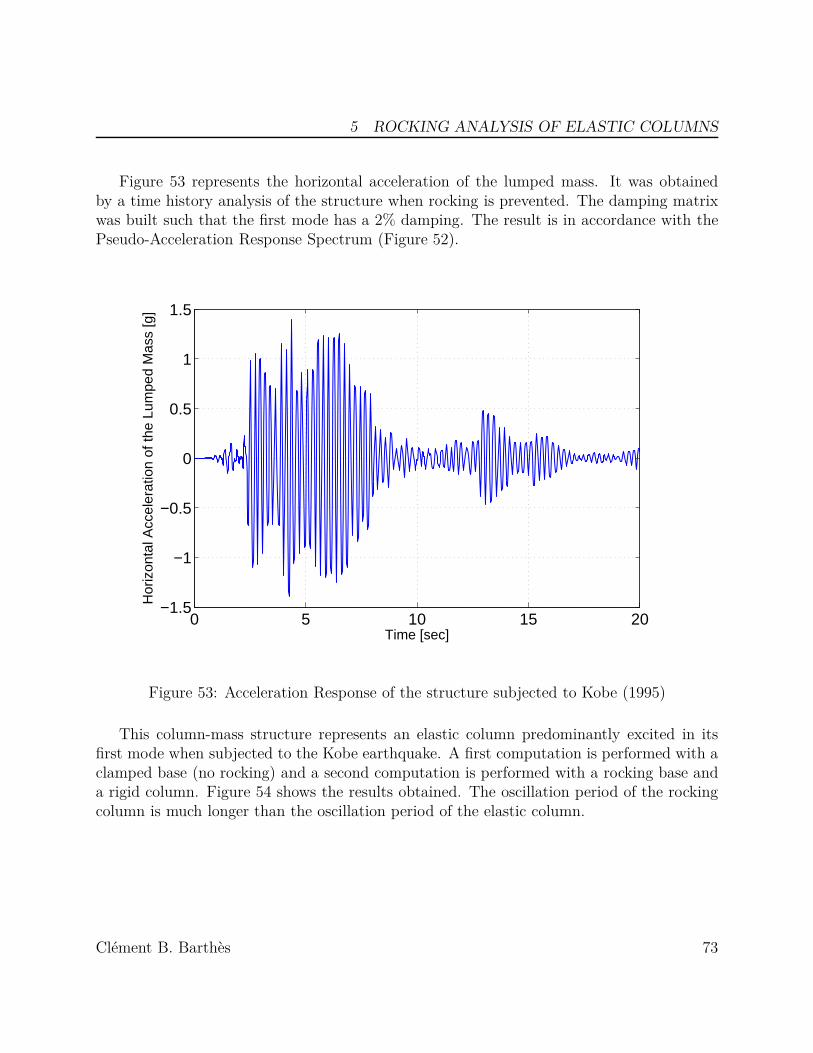
5 ROCKING ANALYSIS OF ELASTIC COLUMNS
Figure 53 represents the horizontal acceleration of the lumped mass. It was obtainedby a time history analysis of the structure when rocking is prevented. The damping matrixwas built such that the first mode has a 2% damping. The result is in accordance with thePseudo-Acceleration Response Spectrum (Figure 52).
0 5 10 15 20−1.5
−1
−0.5
0
0.5
1
1.5
Time [sec]
Hor
izon
tal A
ccel
erat
ion
of th
e Lu
mpe
d M
ass
[g]
Figure 53: Acceleration Response of the structure subjected to Kobe (1995)
This column-mass structure represents an elastic column predominantly excited in itsfirst mode when subjected to the Kobe earthquake. A first computation is performed with aclamped base (no rocking) and a second computation is performed with a rocking base anda rigid column. Figure 54 shows the results obtained. The oscillation period of the rockingcolumn is much longer than the oscillation period of the elastic column.
Clément B. Barthès 73

5 ROCKING ANALYSIS OF ELASTIC COLUMNS
0 5 10 15 20 25 30 35 40−3
−2
−1
0
1
2
3
Time [sec]
Col
umn
Drif
t Rat
io [%
]
Non−rocking base − Elastic ColumnRocking base − Rigid Column
Figure 54: Displacement Response of a Clamped Elastic Column and a Rocking Rigid Col-umn - Kobe (1995)
Clément B. Barthès 74

5 ROCKING ANALYSIS OF ELASTIC COLUMNS
Currently, the rocking behavior is represented by a rigid block model, as presented inChapter 3. Hence the interaction between the rocking rotation and the elastic deformationscan not be computed. The rocking element presented in Chapter 4 can represent such in-teraction. It is proposed here to focus on the importance of such interaction in order to beable to judge if it can further be neglected. Figure 55 represents the rocking base rotationsof a rigid column and of an elastic column. Both columns, detailed in Table 3, were allowedto rock and they both had the same rocking base. The base rotation of the elastic column isslightly less than the base rotation of the rigid column. Furthermore, the number of rockingimpacts is greatly reduced for the elastic column. For the elastic column, the kinetic energyaccumulated while the column was returning to its initial position is partially transformedin bending energy. Hence the rocking rotations are reduced when the column is elastic androcking is more likely to be interrupted.
0 2 4 6 8 10 12 14 16 18 20−0.2
−0.1
0
0.1
0.2
Time [sec]
Roc
king
Bas
e R
otat
ion
θ/α
Rigid ColumnElastic Column
Figure 55: Base Rotations of a Rigid Column and an Elastic Column When Subjected toKobe EQ(1995)
Clément B. Barthès 75
5 ROCKING ANALYSIS OF ELASTIC COLUMNS
5.3 DampingIn Chapter 4, the rigid block is replaced with a very stiff elastic column in order to comparethe results with the rigid block model. The impact generates a fast shock wave as well ashigh-frequency numerical noise in the angular velocity. The HHT integration scheme waschosen in order to filter out these high frequencies. The integration scheme reduces the noisein the high-frequency range. Such technique is considered to be a numerical trick, whereasviscous damping is oftentimes considered more realistic; such statement, however, is arguablesince the viscous damping is usually built with respect to the global response of a structureand has nothing to do with material properties. Therefore, both can be considered as aconvenient numerical tool and they do not model a physical property of the model. It isproposed here to study the viscous damping calibration for a free rocking column.
Equation 33 represents the Rayleigh damping matrix. The parameters a0 and a1 arecalibrated to match given damping ratios of the first two modes of the structure [5].
C = a0 · M + a1 · K (33)At first, a damping matrix proportional to the mass matrix will be computed. A column
subjected to free rocking rotation is modeled. Its properties are summarized in Table 3, butthe Young Modulus is equal to 10Es. The modal analysis must be performed at rest because,if the rocking element is active, the first mode is complex. So the displacement vector is setto zero and the rocking surface is inactive. It is equivalent to a modal analysis of a clampedcolumn. The parameter a0 is chosen such that the first mode of the column has a dampingratio of 2%. Figure 56 shows the result obtained. The period of rocking is significantlylonger than the period of the undamped system. Since the masses are lumped at the nodes,the mass matrix and the damping matrix are diagonal. Hence, if the structure undergoesrigid body motion, the mass-proportional damping matrix will damp it. Such issue is oftenencountered in contact mechanics. When a deformable object is subjected to very large rigidbody displacements, this motion must be undamped in order to remain realistic. Therefore,a mass-proportional damping matrix is not suitable for the problem studied here.
A stiffness proportional matrix is now considered. The parameter a1 is chosen to dampthe first mode of the non-rocking structure with a damping ratio of 2%. Note that theconstraints within the rocking element are approximated with a penalty factor and addedto the stiffness matrix. This penalty factor must not contribute to the damping matrixotherwise, the kinematic constraints would be severely damped. Even though the rockingelement contributes to the stiffness matrix, it must be noted that this contribution is dueto the numerical strategy chosen to handle the constraints (penalty method or Augmented
Clément B. Barthès 76

5 ROCKING ANALYSIS OF ELASTIC COLUMNS
0 2 4 6 8 10 12 14 16 18 20−1
−0.5
0
0.5
1
Time [sec]
Bas
e R
otat
ion
θ/α
No DampingDamping Proportional to Initial StiffnessDamping Proportional to Mass
Figure 56: Free Rocking With Constant Damping Matrices
Lagrangian). Unlike other stiffness contribution, they are not associated with material de-formations but with rigid body motion, so they should not be damped. In the algorithm, thestiffness matrix is built by adding each element stiffness matrix. But to build the dampingmatrix, the algorithm substracts the contribution of the rocking element from the stiffnessmatrix before computing Equation 33. Figure 56 shows the result obtained. The rockingperiod is extremely longer than the rocking period of the undamped system. Thus, thisdamping matrix is also not adequate. It was chosen to be proportional to the stiffnessmatrix, but this stiffness matrix is constantly updated to respect the corotational transfor-mations, whereas the damping matrix remains constant. Here, the rigid body motion isagain disturbed by the damping matrix. In order to avoid such issue, the damping matrixmust also be updated. The parameter a1 remains constant but, for each increment and foreach iteration, the damping matrix is now updated proportionally to the stiffness matrix.Again, the contribution of the rocking element to the stiffness matrix is substracted becauseit is associated with rigid body motion. Figure 57 represents the solution obtained.
Clément B. Barthès 77
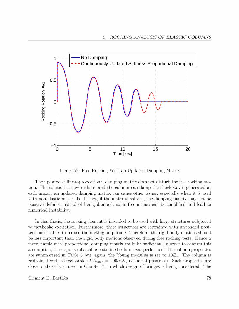
5 ROCKING ANALYSIS OF ELASTIC COLUMNS
0 5 10 15 20−1
−0.5
0
0.5
1
Time [sec]
Roc
king
Rot
atio
n θ
/α
No DampingContinuously Updated Stiffness Proportional Damping
Figure 57: Free Rocking With an Updated Damping Matrix
The updated stiffness-proportional damping matrix does not disturb the free rocking mo-tion. The solution is now realistic and the column can damp the shock waves generated ateach impact an updated damping matrix can cause other issues, especially when it is usedwith non-elastic materials. In fact, if the material softens, the damping matrix may not bepositive definite instead of being damped, some frequencies can be amplified and lead tonumerical instability.
In this thesis, the rocking element is intended to be used with large structures subjectedto earthqake excitation. Furthermore, these structures are restrained with unbonded post-tensioned cables to reduce the rocking amplitude. Therefore, the rigid body motions shouldbe less important than the rigid body motions observed during free rocking tests. Hence amore simple mass proportional damping matrix could be sufficient. In order to confirm thisassumption, the response of a cable-restrained column was performed. The column propertiesare summarized in Table 3 but, again, the Young modulus is set to 10Es. The column isrestrained with a steel cable (EAcable = 200e6N , no initial prestress). Such properties areclose to those later used in Chapter 7, in which design of bridges is being considered. The
Clément B. Barthès 78

5 ROCKING ANALYSIS OF ELASTIC COLUMNS
damping matrix is calibrated such that the first mode of the structure at rest has a dampingratio of 2%. Figure 58 represents the rocking rotation of the column when subjected to Kobeearthquake.
0 5 10 15 20−0.05
−0.025
0
0.025
0.05
Time [sec]
Roc
king
Rot
atio
n θ
/α
No DampingMass−Proportional Damping
Figure 58: Rocking Rotation of a Cable Restrained Cantilever Column - Kobe EQ (1995)
A shown in Figure 58, even for an earthquake excitation, the mass-proportional matrixsignificantly changes the results. The rotation period is longer than the first harmonic pe-riod of the structure used to calibrate the damping matrix. Hence even though the rockingrotations remain small, they are severely damped.
The use of a continuously updated stiffness-proportional damping matrix was also inves-tigated but, as explained earlier, this type of damping matrix can be non positive-definiteand generate numerical instability. Indeed, with such damping matrix, the algorithm failedto converge for this example.
Clément B. Barthès 79

5 ROCKING ANALYSIS OF ELASTIC COLUMNS
Although viscous damping is used in structural engineering to represent the energy dissipa-tion of a structure, if this energy dissipation was only viscous, then a factor associated withthe strain rate ε could be specified for a given material. Instead, the Rayleigh damping ma-trix is calibrated based on the first few modes of the entire structure; hence a1 is defined for agiven structure and not for a given material. Therefore, viscous damping is calibrated usingan empirical approach. It is proven to be very convenient for most structural engineeringapplications but, since it is not founded on physical ground, its reliability must be verifiedfor each application. In order to limit the elastic oscillations of large deformable structures,viscous damping is essential. In Chapter 6 and Chapter 7 a 2% mass-proportional viscousdamping was used. This damping matrix is necessary to damp the elastic oscillations, but itmust be noted that, when the rocking rotations become very large, the damping will generateinaccurate results.
Clément B. Barthès 80

5 ROCKING ANALYSIS OF ELASTIC COLUMNS
5.4 The effect of elastic deformations on rocking behaviorIn Chapter 3, it was shown that, when a rigid block rocks, some energy is lost during impact.This energy must be dissipated in order to respect the conservation of angular momentum,hence the rigid block is assumed to be capable of absorbing it during the impact. Thismodel, presented by Housner in 1963 [16], is now used in most papers to describe rockingbehavior. It is very useful to represent stiff objects such as equipment or large constructionblocks [37]. Indeed, the harmonic oscillations generated by the impact are much faster thanthe rocking oscillations, hence the shock wave is quickly damped and elastic deformationsare negligible. But the behavior of a free rocking elastic column with a lumped mass may bedifferent. Such column may undergo very large elastic deformations, hence their combinedrocking and flexural motion may be complex.
In order to observe the effect of elasticity, three columns are modeled. The columns havethe properties described in Table 3, but each one has a different Young modulus: Es, 10Es
and 15Es. All three columns are undergoing free rocking motion with the same initial angle.There is no viscous damping and the HHT parameter is set to α = −1/12 in order to pre-serve the high frequencies oscillations. In fact, when α tends to zero, the HHT integrationscheme does no longer filter out the high frequencies, when α = −1/12, it may compromisethe stability but, in this example, it is essential to capture accurately the column’s bendingoscillations. In the other examples studied in this thesis, α = −1/6 in order to favour ro-bustness.
Clément B. Barthès 81

5 ROCKING ANALYSIS OF ELASTIC COLUMNS
0 5 10 15 20 25
0
0 5 10 15 20 25−1
0
1
Roc
king
Rot
atio
n θ/
α
0 5 10 15 20 25−1
0
1
Time [sec]
10Es
Es
15Es
Figure 59: Free Rocking of a Column for Different Young’s Moduli
Figure 59 shows the results obtained for the same initial angle with different Young mod-uli. It is observed that the stiffer the column, the longer it rocks. Eventually, the columnis stiff enough to converge towards the rigid block solution. This is an important difference,when compared with the results obtained in Chapter 3. An elastic column rocking on a rigidsurface may suddenly stop rocking. In fact, the kinetic energy due to the rocking motion istransformed into bending energy, which prevents uplift. Hence, instead of creating a rota-tion around the opposite corner, the column simply stops rocking. Figure 59 also shows thatthe period of rocking and its amplitude are the same for each column, regardless of theirstiffness. It is interesting to note that a rigid column and an elastic column whose geometricproperties are the same will rock the same way but that the elastic column will stop rockingwhereas the rigid column will not.
Figures 60 and 61 represent the horizontal tip displacement of the column when the Youngmodulus is equal to respectively Es and 10Es. It can be observed that, when the rocking
Clément B. Barthès 82

5 ROCKING ANALYSIS OF ELASTIC COLUMNS
stops, the column oscillates. The amplitude after the rocking interruption is much smallerbecause there is no more rigid body motion at the base of the column. But the rockingkinetic energy leads to bending oscillations. In Figure 61, it can be noted that the bendingoscillations are dissipated but not in Figure 60. This is because the bending oscillations inFigure 61 are faster and the HHT integration scheme only filters the high frequnecies.
0 5 10 15 20 25−1
−0.75
−0.5
−0.25
0
0.25
0.5
0.75
1
Time [sec]
Tip
Dis
plac
emen
t [m
]
Es
Figure 60: Tip Displacement of an Elastic Rocking Beam with Young Modulus equal to Es
Clément B. Barthès 83

5 ROCKING ANALYSIS OF ELASTIC COLUMNS
0 5 10 15 20 25−1
−0.75
−0.5
−0.25
0
0.25
0.5
0.75
1
Time [sec]
Tip
Dis
plac
emen
t [m
]
10Es
Figure 61: Tip Displacement of an Elastic Rocking Beam with Young Modulus equal to10Es
Clément B. Barthès 84

5 ROCKING ANALYSIS OF ELASTIC COLUMNS
It is proposed to evaluate the amplitude of the bending oscillations due to the rockinginterruption. Several approximations will be made to build the simplified model. The col-umn is modeled as an Euler-Bernoulli beam with linear geometry. The axial deformationsare neglected and only the lumped mass is represented. Figure 62 represents the simplifiedmodel used here. The last rocking rotation observed is called θr
last. It represents the maxi-mum rotation before the last impact; there is no angular velocity in this instance.
Last Rocking Rotation
Maximum Bending Deflection After
Rocking Interruption
Lumped mass
O
Umax
h
2R
Figure 62: Simplified Model of an Elastic Rocking Beam
The column rotates around point O before impact and lands on its base. It is consideredthat the landing does not radiate energy, so the energy is conserved. The kinetic energy dueto rocking is written in Equation 34
Clément B. Barthès 85

5 ROCKING ANALYSIS OF ELASTIC COLUMNS
Erocking =12
I0θ2impact (34)
In order to compute the angular velocity at impact θimpact, the equation of motion (2)described in Chapter 3 has to be solved. It is proposed to linearize it for (α−θ), as explainedby Housner [16]. It gives Equation (35) with p2 = mg
√R2+h2
I0and α, the angle representing
the aspect ratio (α = arctan(Rh
)).
θ − p2θ = −p2α (35)
Equation (36) is obtained by solving Equation (35) for θ(0) = θrlast (the last rocking
rotation observed) and ˙θ(0) = 0.
θimpact = −p√
α2 − (α − θrlast)2 (36)
Combining Equation (35) and Equation (36), the rocking kinetic energy is expressed withrespect to θr
last in Equation (37).
Erocking = 12
I0p2(α2 − (α − θrlast)2) (37)
It is now proposed to compute the bending energy. Equation (38) describes the deflectedshape of the column. v(x) represents the deflection, and the origin of x is the base of thecolumn. This deflected shape is derived from the general Euler-Bernouilli beam equations,assuming that the base of the column is clamped and no moment is applied at the top. Umax
represents the maximum bending deflection at the top of the column once rocking stops.
v(x) = −Umax
2h3 x3 + 3Umax
2h2 x2 (38)
Equation (39) represents the bending energy of the column.
Ebending = 12
∫ h
0EI
(∂2v
∂x2
)2
dx (39)
Equation 40 is obtained by solving (39) for the deflected shape given in Equation (38).
Ebending =3EI
2h3 U2max (40)
Since Ebending = Erocking, the maximum tip displacement Umax is expressed with respectto θr
last in Equation (41).
Clément B. Barthès 86

5 ROCKING ANALYSIS OF ELASTIC COLUMNS
Umax =√
h3
3EImg
√R2 + h2(α2 − (α − θr
last)2) (41)
In order to confirm that the rocking interruption observed in this chapter can be explainedwith this simplified model, the maximum tip displacement observed after the rocking inter-ruption is compared with the estimated tip displacement obtained with this model.
θrini [rad] Estimated Umax [m] Observed Umax [m] Error
EsI 0.094 5.53e − 2 6.02e − 2 8.1%10EsI 0.056 1.45e − 2 1.59e − 2 8.8%15EsI 0.011 5.7e − 3 5.0e − 3 14%
Table 4: Comparison of the rocking-elastic transition results with the simplified model
Clément B. Barthès 87

5 ROCKING ANALYSIS OF ELASTIC COLUMNS
5.5 ConclusionIn this chapter, the behavior of an elastic beam subjected to rocking was studied. The rock-ing element presented in Chapter 4 allows to represent an elastic beam rocking on its base.It was shown that, when an elastic column subjected to an earthquake rocks, it behavesdifferently from a rigid block (Figure 55).
Viscous damping was discussed in Section 5.3. It was shown that, if the damping matrixis proportional to the mass matrix or to the initial tangent stiffness matrix, the rockingmotion is severely damped and become unrealistic. This is particularly true for very largerocking rotation. Only a continuously updated stiffness-proportional damping matrix canproperly represent the rocking behavior of a column. But such matrix can lead to numericalinstability and should be avoided for complicate problems. Hence it was decided to use amass-proportional damping matrix but only if the rocking rotations remain small. This isusually the case for structures subjected to an earthquake and equipped with a restrainingcable. A mass-proportional damping matrix, however, is not suitable to compute the prob-lems with a large initial rotation such as a free rocking block.
At last, the rocking interruption due to column bending was discussed. It was observedthat, when columns are tilted and allowed to rock freely, the stiffer columns will rock longer.A softer column will land and the rocking kinetic energy will lead to column bending. Asimplified model of the rocking column was presented in order to explain how the rockinginterruption affects the column bending.
Clément B. Barthès 88
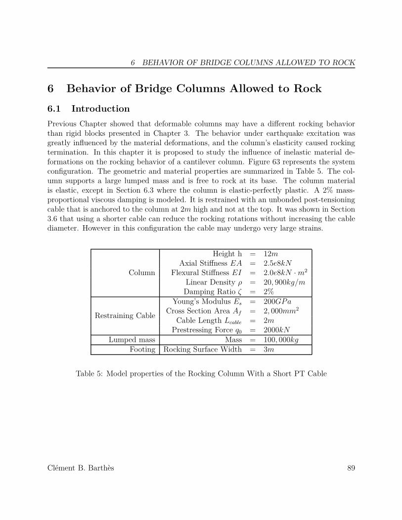
6 BEHAVIOR OF BRIDGE COLUMNS ALLOWED TO ROCK
6 Behavior of Bridge Columns Allowed to Rock
6.1 IntroductionPrevious Chapter showed that deformable columns may have a different rocking behaviorthan rigid blocks presented in Chapter 3. The behavior under earthquake excitation wasgreatly influenced by the material deformations, and the column’s elasticity caused rockingtermination. In this chapter it is proposed to study the influence of inelastic material de-formations on the rocking behavior of a cantilever column. Figure 63 represents the systemconfiguration. The geometric and material properties are summarized in Table 5. The col-umn supports a large lumped mass and is free to rock at its base. The column materialis elastic, except in Section 6.3 where the column is elastic-perfectly plastic. A 2% mass-proportional viscous damping is modeled. It is restrained with an unbonded post-tensioningcable that is anchored to the column at 2m high and not at the top. It was shown in Section3.6 that using a shorter cable can reduce the rocking rotations without increasing the cablediameter. However in this configuration the cable may undergo very large strains.
Column
Height h = 12mAxial Stiffness EA = 2.5e8kN
Flexural Stiffness EI = 2.0e8kN · m2
Linear Density ρ = 20, 900kg/mDamping Ratio ζ = 2%
Restraining Cable
Young’s Modulus Es = 200GP aCross Section Area Af = 2, 000mm2
Cable Length Lcable = 2mPrestressing Force q0 = 2000kN
Lumped mass Mass = 100, 000kgFooting Rocking Surface Width = 3m
Table 5: Model properties of the Rocking Column With a Short PT Cable
Clément B. Barthès 89

6 BEHAVIOR OF BRIDGE COLUMNS ALLOWED TO ROCK
3m
12m
Mas
s
2m
Roc
king
Allo
wed
at
the
base
Fram
e E
lem
ent
Trus
s E
lem
ent
in p
aral
lel
(cab
le)
Roc
king
Ele
men
t
Syst
em C
onfig
urat
ion
Fini
te E
lem
ent M
odel
Figure 63: Cantilever Column with a Short Restraining Cable
Clément B. Barthès 90

6 BEHAVIOR OF BRIDGE COLUMNS ALLOWED TO ROCK
It is first proposed to study the consequences of a failure of the post-tensioning cable.The purpose of this cable is to limit the rocking rotations, hence if it fails the structure mayoverturn. This cable is then replaced with a post-tensioning tie-rod. A cable may undergobrittle failure, but a tie-rod can withstand moderate plastic deformations. However, as thetie-rod yields the initial prestressing force will be reduced hence the column may also over-turn.
Secondly, the yielding of the column is studied. As a cantilever column rocks, it mayexceed its plastic capacity and a plastic hinge will form at the base. This plastic hinge willdissipate energy so it may reduce the rocking rotation. But it will also lead to a larger driftof the lumped mass and may cause the structure to collapse.
Finally, the use of a dissipative fuse connecting the base of the column to the footing isdiscussed. It consists of a mild-steel rod located along the neutral axis of the column. It canwithstand very large plastic deformations in tension and compression. Hence it may help torestrain the rocking rotations and prevent damage of the rest of the structure.
Clément B. Barthès 91

6 BEHAVIOR OF BRIDGE COLUMNS ALLOWED TO ROCK
6.2 Yielding and Failure of the Restraining CableIn this section it is proposed to study the consequences of a cable failure while the structureis rocking. It is impossible to represent the moment-rotation relationship of the rocking ele-ment because it is not governed by a material constitutive law but by kinematic constraintsas explained in 4.2. So instead, Figure 64 represents the restoring moment of the entirestructure versus the rocking rotation, assuming that the structure is rigid. It represents therelationship described in Equation (42), which is derived from the post-tensioned rigid blocksanalysis performed in Section 3.4.1. But in this case the slenderness angle of the structureα = arctan(R
h) is dissociated from the angle αcable arctan( R
hcable), where h is the height of the
column, hcable is the length of the cable and R is half the width of the rocking surface. m andg represent respectively, the lumped mass and the gravity constant. The other parametersη0 and ηα correspond to restraining cable parameters as defined in Chapter 3. They arecalibrated to match the cable properties of the example studied here.
Mr(θ) = m · g ·√
h2 + R2 · (sin(sign(θ)α − θ))
+ m · g ·√
h2cable + R2 · (sign(θ)η0 + (ηalpha − η0) θ
αcablesin(αcable)) (42)
In Figure 64, the dashed red plot represents the static restoring moment of the columnwith a post-tensioning cable and the solid blue plot represents the static restoring momentof the structure once the cable failed. When the column is close to its initial position (i.e.θ is close to zero), the restoring moment is equal to ±4, 000kN · m with the cable and±2, 000kN · m without the cable. Furthermore, without the cable the structure has a soft-ening behavior. So based on the static analysis of this rigid model, it is expected that thecable failure will lead to very large rocking rotations and eventually overturning.
Clément B. Barthès 92

6 BEHAVIOR OF BRIDGE COLUMNS ALLOWED TO ROCK
−1 −0.5 0 0.5 1−20,000
−15,000
−10,000
−5,000
0
5,000
10,000
θ/α
Res
torin
g M
omen
t [kN
⋅m]
Without CableWith Cable
Figure 64: Static Restoring Moment versus θ for a Column assumed to be rigid
Clément B. Barthès 93

6 BEHAVIOR OF BRIDGE COLUMNS ALLOWED TO ROCK
The elastic column presented in Figure 63 is now studied. The post-tensioning cable ismodeled with a truss element. This element cannot be loaded in compression and it mayundergo a brittle failure in tension if the stress exceeds fu = 1, 800MP a. The column issubjected to the Takatori station longitudinal record of the Kobe earthquake (1995).
Figure 65 represents the column’s drift ratio and the cable stress. Only the first 10secof the earthquake response are represented. The maximum drift ratio observed is 7.6%.But due to the viscous damping used in this model, this value is conservative. Actually, inSection 5.3 it was shown that the mass-proportional damping matrix may underestimate therocking rotations when they are too large. So when the cable fails the column’s drift ratiobecomes very large and the column stability may not be preserved.
0 2 4 6 8 10−8
−4
0
4
8
Col
umn
Drif
t Rat
io [%
]
0 2 4 6 8 100
2000
4000
6000
8000
Time [sec]
Cab
le S
tres
s [M
Pa]
Elastic−Brittle Cable fu=1,800MPa
Elastic CableCable Failure
Cable Failure
Figure 65: Drift Ratio of the Column and PT stress with Brittle Cable Failure fu =1, 800MP a - Kobe EQ (1995)
Clément B. Barthès 94
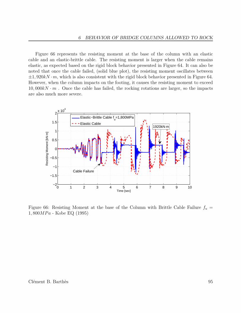
6 BEHAVIOR OF BRIDGE COLUMNS ALLOWED TO ROCK
Figure 66 represents the resisting moment at the base of the column with an elasticcable and an elastic-brittle cable. The resisting moment is larger when the cable remainselastic, as expected based on the rigid block behavior presented in Figure 64. It can also benoted that once the cable failed, (solid blue plot), the resisting moment oscillates between±1, 920kN · m, which is also consistent with the rigid block behavior presented in Figure 64.However, when the column impacts on the footing, it causes the resisting moment to exceed10, 000kN · m . Once the cable has failed, the rocking rotations are larger, so the impactsare also much more severe.
0 1 2 3 4 5 6 7 8 9 10−2
−1.5
−1
−0.5
0
0.5
1
1.5
2x 10
4
Time [sec]
Res
istin
g M
omen
t [kN
⋅m]
Elastic−Brittle Cable fu=1,800MPa
Elastic Cable
Cable Failure
1920kN⋅m
Figure 66: Resisting Moment at the base of the Column with Brittle Cable Failure fu =1, 800MP a - Kobe EQ (1995)
Clément B. Barthès 95

6 BEHAVIOR OF BRIDGE COLUMNS ALLOWED TO ROCK
It is proposed to replace the post-tensioning cable with a tie-rod of the same diameter.This tie-rod (often called Dywidag bar in the industry) has an elastic limit fy = 1, 200MP a[7]. It consists of a solid steel section rod with the same Young modulus than a PT ca-ble (Es = 200GP a). It cannot be loaded in compression but it can withstand moderateplastic deformations in tension. So the elastic-brittle truss element representing the cable isreplaced with an elastic-perfectly plastic truss element. This element has no resisting forcewhen loaded in compression.
Figure 67 shows the structure’s response with an elastic-perfectly plastic tie-rod when itis subjected to Kobe earthquake. Only the first 10sec of the earthquake response are repre-sented. It shows that the prestressing force of the tie-rod is entirely lost at time t = 5sec.Therefore, the column’s drift ratio is larger than the column equipped with an elastic cable.The plastic elongation of the tie-rod increases only if the column’s drift ratio exceeds themaximum amplitude observed at previous time steps. Eventually, the plastic strain of thetie-rod reaches 4%, and it does no longer restrain the rocking rotations. The column’s max-imum drift ratio is 215% higher than the maximum drift ratio of the column equipped withan elastic cable.
Clément B. Barthès 96
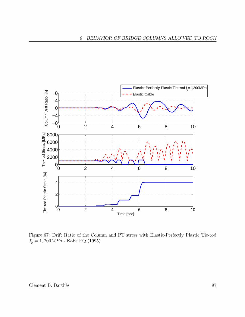
6 BEHAVIOR OF BRIDGE COLUMNS ALLOWED TO ROCK
0 2 4 6 8 10−8
−4
0
4
8
Col
umn
Drif
t Rat
io [%
]
0 2 4 6 8 100
2000
4000
6000
8000
Tie
−ro
d S
tres
s [M
Pa]
Elastic−Perfectly Plastic Tie−rod fy=1,200MPa
Elastic Cable
0 2 4 6 8 100
2
4
Time [sec]Tie
−ro
d P
last
ic S
trai
n [%
]
Figure 67: Drift Ratio of the Column and PT stress with Elastic-Perfectly Plastic Tie-rodfy = 1, 200MP a - Kobe EQ (1995)
Clément B. Barthès 97
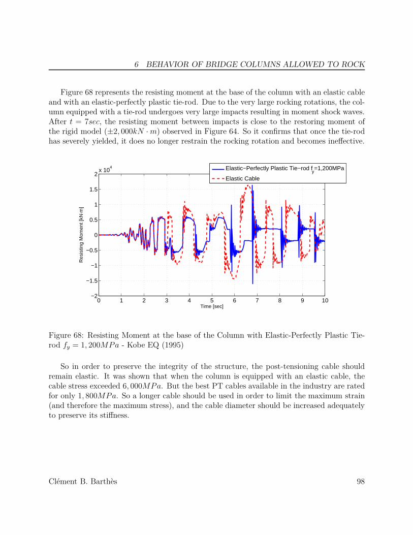
6 BEHAVIOR OF BRIDGE COLUMNS ALLOWED TO ROCK
Figure 68 represents the resisting moment at the base of the column with an elastic cableand with an elastic-perfectly plastic tie-rod. Due to the very large rocking rotations, the col-umn equipped with a tie-rod undergoes very large impacts resulting in moment shock waves.After t = 7sec, the resisting moment between impacts is close to the restoring moment ofthe rigid model (±2, 000kN · m) observed in Figure 64. So it confirms that once the tie-rodhas severely yielded, it does no longer restrain the rocking rotation and becomes ineffective.
0 1 2 3 4 5 6 7 8 9 10−2
−1.5
−1
−0.5
0
0.5
1
1.5
2x 10
4
Time [sec]
Res
istin
g M
omen
t [kN
⋅m]
Elastic−Perfectly Plastic Tie−rod f
y=1,200MPa
Elastic Cable
Figure 68: Resisting Moment at the base of the Column with Elastic-Perfectly Plastic Tie-rod fy = 1, 200MP a - Kobe EQ (1995)
So in order to preserve the integrity of the structure, the post-tensioning cable shouldremain elastic. It was shown that when the column is equipped with an elastic cable, thecable stress exceeded 6, 000MP a. But the best PT cables available in the industry are ratedfor only 1, 800MP a. So a longer cable should be used in order to limit the maximum strain(and therefore the maximum stress), and the cable diameter should be increased adequatelyto preserve its stiffness.
Clément B. Barthès 98

6 BEHAVIOR OF BRIDGE COLUMNS ALLOWED TO ROCK
6.3 Elastic-Perfectly Plastic ColumnIn this section, it is proposed to study the rocking behavior of a column when a plastichinge forms at its base. The column configuration presented in Figure 63 is modeled. Theproperties of the structure are presented in Table 5. The PT cable is assumed to remainelastic. The column’s axial and shear deformations are elastic, but flexure deformations areelastic-perfectly plastic. The plastic capacity of the column is Mp = 6, 000kN · m. Since themoment is maximum at the base of the column, it is expected that a plastic hinge will formas described in Figure 69.
W
E,A,I,
Mp
2R
Figure 69: Elastic Column With a Lumped Mass, a Plastic Hinge and a Rocking Base
Clément B. Barthès 99

6 BEHAVIOR OF BRIDGE COLUMNS ALLOWED TO ROCK
Figure 70 represents the column drift ratio and the rocking rotation at the base of thecolumn for an elastic column and for an elastic-plastic column. First it can be noted thatthe rocking rotations are greatly reduced when a plastic hinge forms at the base (dashedred plot). Figure 71 represents the resisting moment at the base of the column. As ex-pected, the resisting moment of the elastic-plastic column (dashed red plot) never exceedsMp = 6, 000kN · m. Otherwise both plots are very similar, and the plastic hinge does notseem to affect the pattern of the rocking impacts during the earthquake.
0 5 10 15 20 25 30 35 40−3
−2
−1
0
1
2
3
Col
umn
Drif
t Rat
io [%
]
0 5 10 15 20 25 30 35 40−0.2
−0.1
0
0.1
0.2
Time [sec]
Roc
king
Rot
atio
n θ/
α
Elastic Rocking ColumnElastic−Plastic Rocking Column, M
p=6,000kN⋅m
Figure 70: Column Drift Ratio and Rocking Rotation for an Elastic Column and an Elastic-Perfectly Plastic Column - Kobe EQ (1995)
As the rocking rotation increases, the resisting moment at the base of the column alsoincreases because of the PT cable elongation. Eventually, the resisting moment at the baseof the column reaches the plastic capacity Mp, the rocking rotation is bounded and only
Clément B. Barthès 100
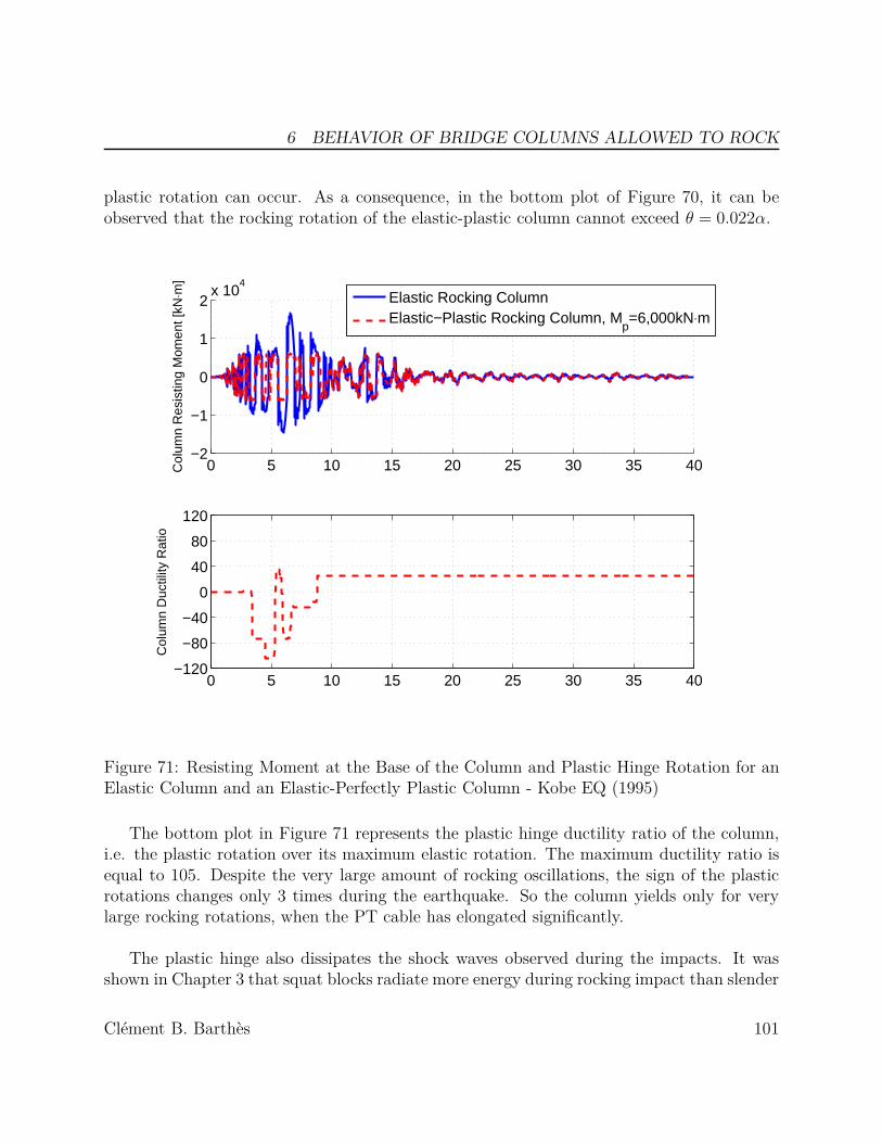
6 BEHAVIOR OF BRIDGE COLUMNS ALLOWED TO ROCK
plastic rotation can occur. As a consequence, in the bottom plot of Figure 70, it can beobserved that the rocking rotation of the elastic-plastic column cannot exceed θ = 0.022α.
0 5 10 15 20 25 30 35 40−2
−1
0
1
2x 10
4
Col
umn
Res
istin
g M
omen
t [kN
⋅m]
Elastic Rocking ColumnElastic−Plastic Rocking Column, M
p=6,000kN⋅m
0 5 10 15 20 25 30 35 40−120
−80
−40
0
40
80
120
Col
umn
Duc
tility
Rat
io
Figure 71: Resisting Moment at the Base of the Column and Plastic Hinge Rotation for anElastic Column and an Elastic-Perfectly Plastic Column - Kobe EQ (1995)
The bottom plot in Figure 71 represents the plastic hinge ductility ratio of the column,i.e. the plastic rotation over its maximum elastic rotation. The maximum ductility ratio isequal to 105. Despite the very large amount of rocking oscillations, the sign of the plasticrotations changes only 3 times during the earthquake. So the column yields only for verylarge rocking rotations, when the PT cable has elongated significantly.
The plastic hinge also dissipates the shock waves observed during the impacts. It wasshown in Chapter 3 that squat blocks radiate more energy during rocking impact than slender
Clément B. Barthès 101

6 BEHAVIOR OF BRIDGE COLUMNS ALLOWED TO ROCK
blocks. Since this column is slender (aspect ratio of 8), the energy radiated by the rockingimpacts is small. Therefore, when a rocking impact occur, the column yields but the plasticrotation does not change significantly.
Overall, the plastic hinge greatly reduces the column’s drift ratio. However, a stronglimitation of the model must be noted. When the plastic hinge forms at the base of thecolumn, the properties of the rocking element remain unchanged. But in practice, when acolumn yields at its base, the local damage may change the rocking properties. This damagemay simply lead to a reduction of the rocking radius, or it may change the shape of therocking surface and cause rolling. Damage on the rocking surface is not investigated in thisthesis and is left for further research.
6.4 Rocking Column with a PT Cable and a Dissipative FuseIt was shown that a PT cable can limit the rocking rotation when the column is subjectedto a moderate earthquake but it may not be sufficient. In fact, a short PT cable may failand a post tensioning tie-rod will become useless after one large rocking rotation as shownin Section 6.2. Therefore, it is proposed in this section to combine the use of a PT cablewith a dissipative fuse. Figure 72 shows the system configuration. The fuse is modeled witha truss element, connecting the base of the column with the footing. Unlike a PT cable, itcan be loaded in tension and compression. Its material properties correspond to a mild-steel,with a low elastic limit and capability of withstanding large plastic cycles. The PT cable isconnected to the top of the column in order to limit its strain when the column rocks. Thesystem properties are summarized in Table 6.
Clément B. Barthès 102

6 BEHAVIOR OF BRIDGE COLUMNS ALLOWED TO ROCK
Mas
s
Roc
king
Allo
wed
at
the
base
Fram
eE
lem
ent
Trus
s E
lem
ent i
n pa
ralle
l(F
use)
Roc
king
Ele
men
t
Syst
em C
onfig
urat
ion
Fini
te E
lem
ent M
odel
Pos
t-Te
nsio
ning
C
able
Dis
sipa
tive
Fuse
Trus
s E
lem
ent i
n pa
ralle
l(C
able
)
Figure 72: Column with an Unbonded Restraining Cable and a Dissipative Fuse
Clément B. Barthès 103

6 BEHAVIOR OF BRIDGE COLUMNS ALLOWED TO ROCK
Column
Height h = 12mAxial Stiffness EA = 2.5e8kN
Flexural Stiffness EI = 2.0e8kN · m2
Linear Density ρ = 20, 900kg/mDamping Ratio ζ = 2%
Restraining Cable
Young’s Modulus Es = 200GP aCross Section Area Ac = 2, 000mm2
Cable Length Lcable = 12mPrestressing Force q0 = 2000kN
Dissipative Fuse
Young’s Modulus Es = 200GP aCross Section Area Af = 16, 000mm2
Fuse Length hfuse = 2000mmIsotropic Hardening Hi = Es
20Elastic Limit fy = 200MP a
Ultimate Strength fu = 1000MP aLumped mass Mass = 100, 000kg
Footing Rocking Surface Width = 3m
Table 6: Model Properties of the Rocking Column With Fuse and PT Cable
Clément B. Barthès 104

6 BEHAVIOR OF BRIDGE COLUMNS ALLOWED TO ROCK
The structure presented in Figure 72 is subjected to the Takatori station longitudinalrecord of the Kobe earthquake (1995). Figure 73 shows the rocking rotations of the column.Only the first 20sec of the earthquake response are represented. When no fuse is used (solidblue line), the rocking rotations are very large. Because the PT cable is anchored at the topof the column, it is less effective than the elastic short cable used previously in this chapter,however, it also prevents the cable to undergo very large strains. When the fuse is added(dashed red plot), the rocking rotations are greatly reduced. Figure 74 shows the resistingmoment at the base of the column. It should be noted that, when the rocking rotations arelarge, the resisting force of the dissipative fuse causes the resisting moment at the column’sbase to increase. However, the maximum moment observed is larger for the column with nofuse because the rocking impacts cause very large shock waves at the base. Hence, in thisexample when a fuse is used, the resisting moment at the base of the column and the rockingrotations are reduced.
0 2 4 6 8 10 12 14 16 18 20−0.4
−0.3
−0.2
−0.1
0
0.1
0.2
0.3
0.4
Time [sec]
Roc
king
Rot
atio
n θ/
α
Without FuseWith Fuse
Figure 73: Rocking Rotation of a Column with an Unbonded Restraining Cable and aDissipative Fuse - Kobe (1995)
Clément B. Barthès 105

6 BEHAVIOR OF BRIDGE COLUMNS ALLOWED TO ROCK
0 5 10 15 20−2.5
−2
−1.5
−1
−0.5
0
0.5
1
1.5
2
2.5x 10
4
Time [sec]
Res
istin
g M
omen
t [kN
⋅m]
Without FuseWith Fuse
Figure 74: Resisting Moment at the Base of a Column With an Unbonded Restraining Cableand a Dissipative Fuse - Kobe (1995)
Clément B. Barthès 106

6 BEHAVIOR OF BRIDGE COLUMNS ALLOWED TO ROCK
An unexpected behavior can be observed after time t = 10sec in Figure 73. The columnwith a fuse continues to rock, whereas the column that is not equipped with a fuse stopsrocking. The role of the fuse is to restrain rocking rotation, so why a fuse can cause rockingto occur when a column without a fuse does not rock at all?
This contradiction can be explained by analyzing the consequences of the plastic elonga-tion of the fuse. When the column is uplifted, the fuse yields in tension and restrains therocking rotation as shown in Figure 75, but, when the column returns to its initial position,the fuse is now loaded in compression due to the plastic elongation that occured previously.Hence the fuse acts against the weight of the structure and prevents the rocking surface toclose. This is confirmed with the fuse response presented in Figure 76. The resisting forceof the fuse is normalized with respect to the total weight of the structure added with theprestressing force of the PT cable (P + W = 1392kN). It shows that the fuse is alternatelyloaded in tension and compression and, after time t = 16sec, the normalized resisting forceis always less than −1. In other words, after time t = 16sec, the weight of the structureand the prestressing force are entirely supported by the fuse and the rocking element is intension. Consequently, the structure cannot return to its initial position and remains tiltedtoward one side. This is confirmed in Figure 73 where, after t = 16sec, the rocking rotationremains negative.
Clément B. Barthès 107

6 BEHAVIOR OF BRIDGE COLUMNS ALLOWED TO ROCK
Whe
n th
e co
lum
n up
lifts
, the
fuse
yi
elds
in te
nsio
n an
d re
stra
in
rock
ing
rota
tion
Whe
n th
e co
lum
n re
turn
s to
its
initi
al
posi
tion,
the
fuse
is n
ow lo
aded
in
com
pres
sion
and
pre
vent
s th
e ro
ckin
g su
rface
to c
lose
Fuse
Figure 75: The Fuse Prevents the Column to Return to its Initial Position
Clément B. Barthès 108

6 BEHAVIOR OF BRIDGE COLUMNS ALLOWED TO ROCK
0 5 10 15 200
0.2
0.4
0.6
0.8
Fus
e P
last
ic S
trai
n [%
]
0 5 10 15 20−5−4−3−2−1
012345
Time [sec]
Nor
mal
ized
Fus
e F
orce
Figure 76: Fuse Resisting Force Normalized with Respect to the Weight of the Structureadded with the Prestressing Force of the PT Cable and Fuse Plastic Strain for a ColumnWith an Unbonded Restraining Cable and a Dissipative Fuse - Kobe (1995)
Clément B. Barthès 109
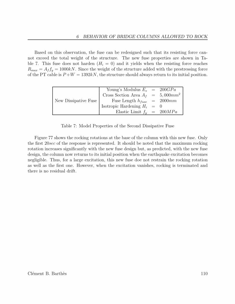
6 BEHAVIOR OF BRIDGE COLUMNS ALLOWED TO ROCK
Based on this observation, the fuse can be redesigned such that its resisting force can-not exceed the total weight of the structure. The new fuse properties are shown in Ta-ble 7. This fuse does not harden (Hi = 0) and it yields when the resisting force reachesRmax = Af fy = 1000kN . Since the weight of the structure added with the prestressing forceof the PT cable is P +W = 1392kN , the structure should always return to its initial position.
New Dissipative Fuse
Young’s Modulus Es = 200GP aCross Section Area Af = 5, 000mm2
Fuse Length hfuse = 2000mmIsotropic Hardening Hi = 0
Elastic Limit fy = 200MP a
Table 7: Model Properties of the Second Dissipative Fuse
Figure 77 shows the rocking rotations at the base of the column with this new fuse. Onlythe first 20sec of the response is represented. It should be noted that the maximum rockingrotation increases significantly with the new fuse design but, as predicted, with the new fusedesign, the column now returns to its initial position when the earthquake excitation becomesnegligible. Thus, for a large excitation, this new fuse doe not restrain the rocking rotationas well as the first one. However, when the excitation vanishes, rocking is terminated andthere is no residual drift.
Clément B. Barthès 110

6 BEHAVIOR OF BRIDGE COLUMNS ALLOWED TO ROCK
0 2 4 6 8 10 12 14 16 18 20−0.4
−0.3
−0.2
−0.1
0
0.1
0.2
0.3
0.4
Time [sec]
Roc
king
Rot
atio
n θ/
α
Without FuseWith the Initial Fuse DesignWith the New Fuse Design
Figure 77: Rocking Rotation of a Column with an Unbonded Restraining Cable and theNew Dissipative Fuse - Kobe (1995)
Clément B. Barthès 111

6 BEHAVIOR OF BRIDGE COLUMNS ALLOWED TO ROCK
Figure 78 shows the PT cable stress during the earthquake excitation. It shows thatthe cable stress is greatly reduced when a fuse is used. This is an expected result since thecable strain depends on the amplitude of the rocking rotation, and the fuse does restrain therocking rotations. Hence the PT cable stress is also reduced since the cable is linear elastic.
0 2 4 6 8 10 12 14 16 18 200
500
1000
1500
2000
Time [sec]
Cab
le S
tres
s [M
Pa]
Without FuseWith the Initial Fuse DesignWith the New Fuse Design
Figure 78: PT Cable Stress for a Column With an Unbonded Restraining Cable and aDissipative Fuse - Kobe (1995)
The results presented in this section show that the dissipative fuse is an effective deviceto reduce the amplitude of the rocking rotations. It also damps the rocking impacts thus,as a result, the resisting moment at the base of the column is not disturbed by shock waves.However, when the fuse undergoes plastic elongation and returns to its initial position, it maybe loaded in compression. At the end of the earthquake excitation, if the residual force inthe fuse is greater than the weight of the structure, then the column may have a residual drift.
Clément B. Barthès 112

6 BEHAVIOR OF BRIDGE COLUMNS ALLOWED TO ROCK
6.5 ConclusionIn this chapter, the rocking behavior of a column equipped with a PT cable and subjected tonon-elastic deformations was studied. At first, the failure of the PT cable was investigated.It was shown that it can lead to extremely large column’s drift ratio. Hence, if a cable isused, its capacity must be such that no failure can occur when the structure is subjectedto a severe earthquake. It was then proposed to replace the post-tensioning cable with aprestressing tie-rod. These tie-rods have a lower strength but they can undergo moderateplastic deformations. The yielding of the tie-rods, however, was also very penalizing. Evena reasonable plastic deformation leads to a total loss of the prestressing load. Furthermore,once the tie-rod yields due to a large rocking rotation, it becomes slack and ineffective, asshown in Figure 67. It was shown in Chapter 3 that the initial post-tensioning force cancontrol the rocking initiation, whereas the cable stiffness may have the advantage to keeprocking rotation low. Since bridge columns are usually slender, the use of a PT cable is es-sential. In this chapter, however, it was shown that to preserve the integrity of the structure,the PT cable should remain elastic. Hence instead of using a short cable anchored near thebase of the column, it may be necessary to use a longer cable with a larger diameter that isanchored at the top of the column.
Secondly, a plastic hinge forming at the base of a rocking column was studied. One con-cern was that the rocking rotation cumulated with the plastic hinge rotation would lead tothe overturning of the structure but it turned out that, once a plastic hinge was formed at thebase of the column, the overall drift ratio was reduced. The kinetic energy due to rocking wasdissipated by the permanent rotations of the plastic hinge. Therefore, the rocking rotationswere greatly reduced and the structure remained stable despite the plastic hinge rotation.It must be noted, however, that despite the plastic hinge rotation forming at the base ofthe column, the properties of the rocking element were assumed to remain unchanged. Inpractice, it is likely that, when damage occurs at the base of the column, the geometry of therocking surface will change. This issue is not discussed in this thesis and is left for furtherresearch.
Finally, the use of a dissipative fuse at the base of the column was studied. As expected,it helped to reduce the amplitude of the rocking rotation during a large earthquake excita-tion. A curious behavior, however, was discovered. When the column returns to its initialposition, the elongated fuse may prevent the rocking surface to close and rocking rotationsmay continue even for a minor earthquake excitation. This issue was explained in detailsin Section 6.4. Overall, the use of a fuse combined with a PT cable was very effective torestrain the rocking rotation, but it may cause the structure to have a residual drift afterthe earthquake excitation if the fuse is too strong.
Clément B. Barthès 113

6 BEHAVIOR OF BRIDGE COLUMNS ALLOWED TO ROCK
Clément B. Barthès 114

7 BEHAVIOR OF BRIDGES WITH ROCKING COLUMNS
7 Behavior of Bridges with Rocking Columns
7.1 IntroductionThe behavior of a deformable rocking column was studied in Chapter 5. Interaction betweenthe rocking behavior and the deformations of the column was observed. Chapter 6 focusedon the behavior of the structure when permanent deformations occur with rocking and it wasshown that a cable failure must be avoided. Hence it was preferred to leave the restrainingcable unbonded along the entire height of the column in order to reduce the cable elongationduring rocking. Furthermore, it was proposed to use a mild-steel fuse at the base of thecolumn in order to dissipate energy during rocking and enhance stability.
The use of rocking footing for bridge columns was studied by Kwan and Billington in [20]and [21] and rocking foundations were studied by S. Gajan and B. L. Kutter [12]. A rockingfooting may be unavoidable in precast construction. Since the reinforcing steel cannot beeasily connected at the prefabricated elements interface, only a post-tensioning cable is usedto hold the elements together. In this thesis the columns are intentionally allowed to rock,in order to mitigate the harmonic excitation of the structure. To facilitate rocking on thefooting, the connection between the top of the column and the superstructure is also allowedto rock.
In this chapter, the behavior of two bridge configurations is investigated. The firstconfiguration is a single-column bridge with two symmetric spans. At the abutments, thegirder is free to rotate and translate longitudinally. The second configuration is a three-spanbridge with two columns having different height with the same cross-section; thus, the twocolumns have a different aspect ratio. The bridge columns are allowed to rock at both ends.They are restrained with an unbonded PT cable anchored at the footing and the girder. Foreach bridge configuration, the behavior of three types of column connections are studied:
• Columns monolithically connected to the girder and the footing
• Columns allowed to rock at both ends and restrained with a PT cable
• Columns allowed to rock at both ends and restrained with a PT cable and a dissipativefuse at the base.
Clément B. Barthès 115

7 BEHAVIOR OF BRIDGES WITH ROCKING COLUMNS
The first bridge configuration is represented in Figure 79. The girder is free to rotateand translate horizontally at the abutments but rocking is not allowed. A rocking element isplaced at the top and the bottom joint of the column. The column is post-tensioned betweenthe footing and the bridge deck, using an unbonded cable with a length equal to the columnheight. One of the column connections studied in this chapter will be equipped with a fuse.This fuse is modeled, using a truss element with a corotational geometry description. It isconnected with the footing and the bottom of the column, at a height of 1m. No fuse isused at the top in order to make sure that the column’s resisting moment remains belowthe girder’s moment capacity. A fuse at the base of the column may also prevent it fromslipping on its footing.
RockingElements
Figure 79: Single Column Bridge Configuration
Clément B. Barthès 116

7 BEHAVIOR OF BRIDGES WITH ROCKING COLUMNS
The second bridge studied consists of a two columns structure. The abutment spans areof equal length and the left column is twice as high as the right column. Seismic resistancedesign of short columns is challenging. Indeed, a short column may undergo a brittle failurein shear. Even with a very large amount of transversal reinforcements, it may be very diffi-cult to avoid a shear failure mode. Note that fiber elements cannot properly represent shearfailure. Instead, the demand in shear observed during computation is used a posteriori tochoose the appropriate amount of transversal steel reinforcement.
It is expected that allowing the column to rock will prevent shear failure. However, sinceboth columns have a different aspect ratio, they have a different rocking behavior. A com-plicate rocking interaction will occur between these two columns due to their connection tothe same girder.
Rocking Elements
Figure 80: Two-Columns Bridge Model
Properties of both bridges are summarized in Table 8. Figure 81 depicts the designoutlines. The abutment supports are simple rollers, allowing the girder to translate longi-tudinally. A rocking element is inserted between the columns and the footings as well asbetween the columns and the girder. A post-tensioning cable anchored between the girderand the footing prevents the column from overturning. Furthermore, a dissipative fuse isinserted at the base of the column connected to the footing. No fuse is installed between thetop of the column and the girder.
Clément B. Barthès 117

7 BEHAVIOR OF BRIDGES WITH ROCKING COLUMNS
Single Column Bridge Two-Columns BridgeColumn Height 24m 24m and 12mColumn Weight 4, 920kN 4, 920kN and 2, 460kN
Girder length 80m 120mGirder Weight 11, 772kN 15, 696kN
Abutment spans 40m 35mCentral span na 50m
Table 8: Bridges Dimensions
Only the in-plane displacements are allowed, hence the structure can not deform laterally.The columns and the girder were modeled using corotational beam elements embedded inFEDEASLab. The geometric and material properties of the structure are presented in Table9. The bridge properties were obtained from Ketchum et al. [18] report, which representa typical CalTrans highway bridge. CalTrans often designs bridge columns with a circularsolid section in order to optimize the concrete confinement. In this Chapter, it is proposed touse a hollow square section in order to accommodate the PT cable and the fuse. Column sizeand reinforcement are proposed based on experience developed in Chapter 6. The outcomeof the analyses conducted in this chapter will indicate the column force design values.
Clément B. Barthès 118

7 BEHAVIOR OF BRIDGES WITH ROCKING COLUMNS
RockingConnections
RestrainingCable
Fuse
#32 M #16 M@35mm
3m 1.4m
Elevation
Cross-Section
Figure 81: Drawing Outline of the Column Connections with its Footing and the Super-structure
Clément B. Barthès 119

7 BEHAVIOR OF BRIDGES WITH ROCKING COLUMNS
Column
Width b = 3md = 3m
Wall Thickness = 0.8mDetailed Properties in Table 10
Girder
Young Modulus = 40e9N/m2
Cross Section = 5m2
I = 3.5m4
Density = 2.5e3kg/m3
Cable
Young Modulus = 200GP aCross Section Area = 5, 000mm2
Prestressing force = 2000kNUltimate Strength fu = 1800MP a
Dissipative Fuse
Young Modulus = 200GP aCross Section Area Af = 5, 000mm2
Yielding Strength fy = 200MP aIsotropic Hardening Modulus Hi = 20MP a
Rocking Elements Rocking Width 2R = 3m
Table 9: Bridge properties
The cable properties are chosen to meet several requirements. First, it has to allow rock-ing but restrain its amplitude. Secondly, it must not fail, even for a large rocking rotation.Therefore, its initial prestressing load is only 20% of the weight supported by the column.As explained in Chapter 3, a low initial prestessing force will allow the structure to rockfor a low earthquake excitation, hence limit the demand on the column. Furthermore, thecable length and diameter were chosen such that the cable will not fail if the rocking rota-tion at the base of the tall column remains below 80% of the slenderness angle of that column.
The fuse properties are presented in Table 9. Its yielding capacity is 1, 000kN and itshardening modulus is very low (Hi
Es= 1e − 4). The total resisting force at the base of the
column (Weight and PT cable force) is equal to 12, 806kN so the ratio between the fusecapacity and the vertical load is 8.33%. Based on the findings presented in Section 6.4, thecapactiy of the fuse is sufficiently low to prevent any residual drift.
Clément B. Barthès 120
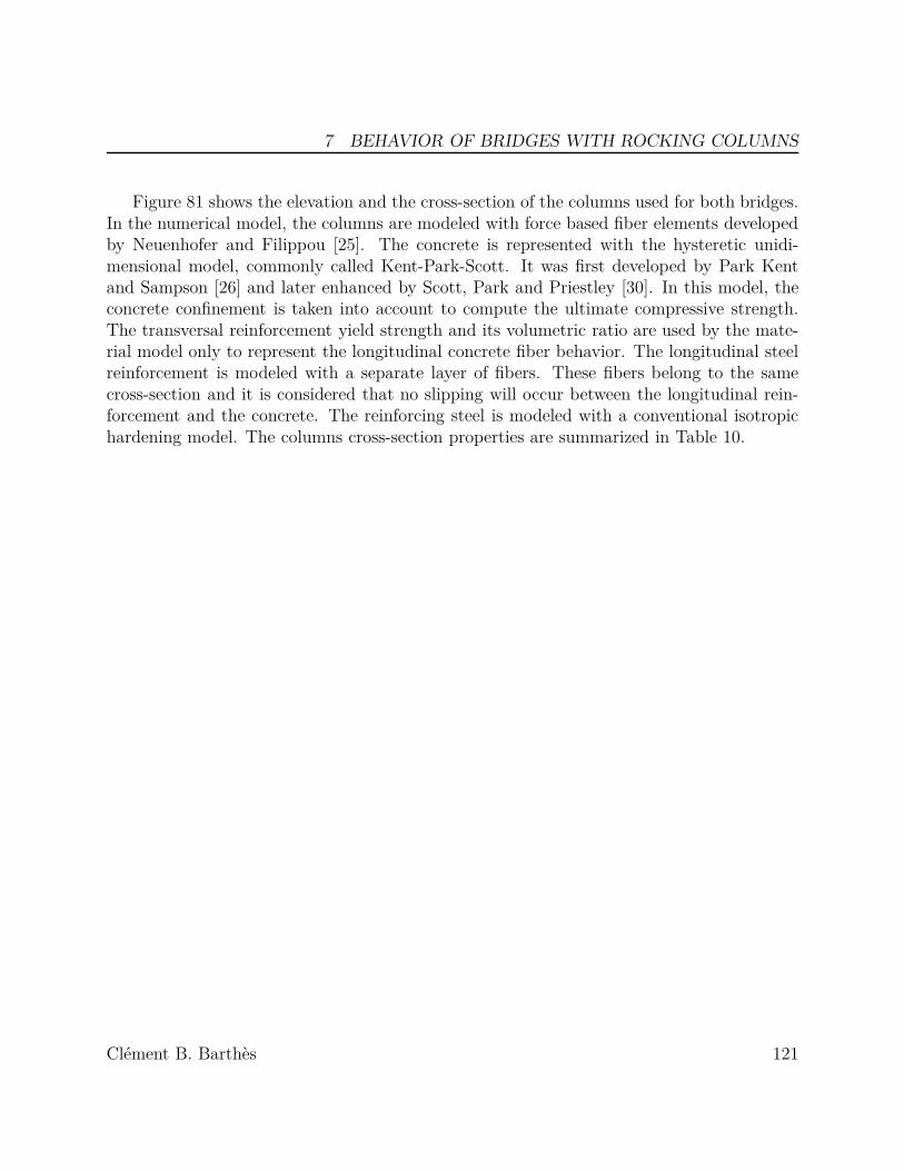
7 BEHAVIOR OF BRIDGES WITH ROCKING COLUMNS
Figure 81 shows the elevation and the cross-section of the columns used for both bridges.In the numerical model, the columns are modeled with force based fiber elements developedby Neuenhofer and Filippou [25]. The concrete is represented with the hysteretic unidi-mensional model, commonly called Kent-Park-Scott. It was first developed by Park Kentand Sampson [26] and later enhanced by Scott, Park and Priestley [30]. In this model, theconcrete confinement is taken into account to compute the ultimate compressive strength.The transversal reinforcement yield strength and its volumetric ratio are used by the mate-rial model only to represent the longitudinal concrete fiber behavior. The longitudinal steelreinforcement is modeled with a separate layer of fibers. These fibers belong to the samecross-section and it is considered that no slipping will occur between the longitudinal rein-forcement and the concrete. The reinforcing steel is modeled with a conventional isotropichardening model. The columns cross-section properties are summarized in Table 10.
Clément B. Barthès 121

7 BEHAVIOR OF BRIDGES WITH ROCKING COLUMNS
Fibers layoutConcrete = 15fibers
Longitudinal Steel Reinforcements = 4fibersFiber Integration Rule = Midpoint
Elements layout
Geometric Description = CorotationalIntegration Points = 5
Maximum Integration Points Subdivision = 5Element Integration Rule = Gauss-Lobatto
Concrete Unconfined Compressive strength fc = 30MP a
Longitudinal Steel
Yielding strength fy = 420MP aYoung Modulus Es = 200GP a
Isotropic Hardening Hi = 10GP aOuter Cross-Section area Aso = 244cm2
Inner Cross-Section area Asi = 147cm2
Transversal SteelYielding strength fy = 420MP a
Stirrups Volumetric Ratio ρs = 0.75%Stirrups spacing at column ends sh = 35mm
Table 10: Column Cross-Section properties
Clément B. Barthès 122
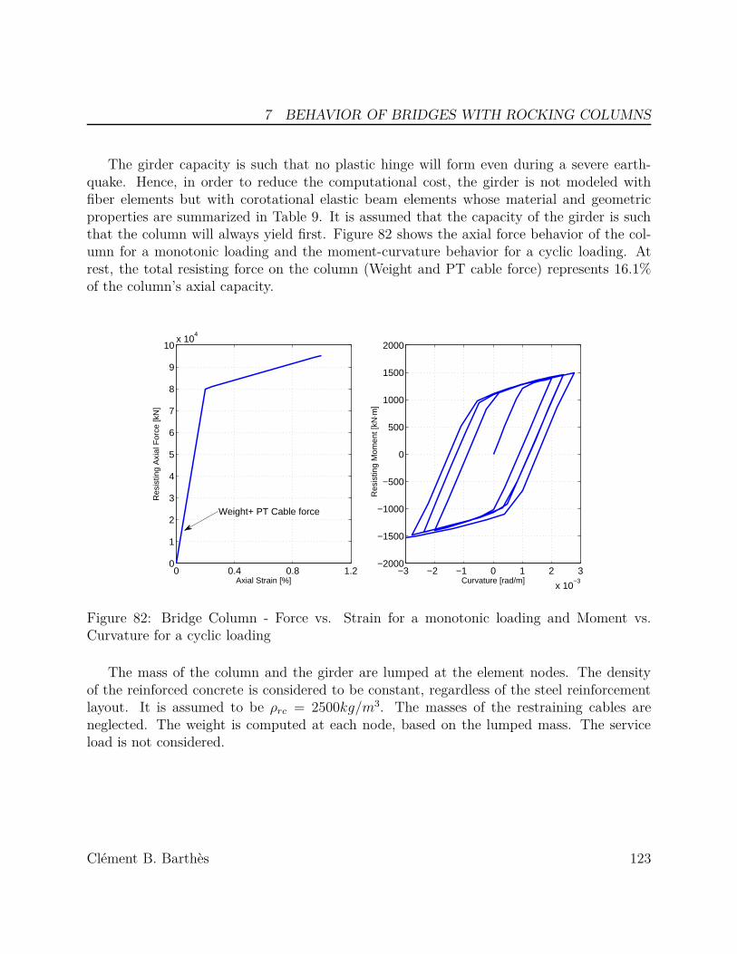
7 BEHAVIOR OF BRIDGES WITH ROCKING COLUMNS
The girder capacity is such that no plastic hinge will form even during a severe earth-quake. Hence, in order to reduce the computational cost, the girder is not modeled withfiber elements but with corotational elastic beam elements whose material and geometricproperties are summarized in Table 9. It is assumed that the capacity of the girder is suchthat the column will always yield first. Figure 82 shows the axial force behavior of the col-umn for a monotonic loading and the moment-curvature behavior for a cyclic loading. Atrest, the total resisting force on the column (Weight and PT cable force) represents 16.1%of the column’s axial capacity.
0 0.4 0.8 1.20
1
2
3
4
5
6
7
8
9
10x 10
4
Axial Strain [%]
Res
istin
g A
xial
For
ce [k
N]
−3 −2 −1 0 1 2 3
x 10−3
−2000
−1500
−1000
−500
0
500
1000
1500
2000
Curvature [rad/m]
Res
istin
g M
omen
t [kN
⋅m]
Weight+ PT Cable force
Figure 82: Bridge Column - Force vs. Strain for a monotonic loading and Moment vs.Curvature for a cyclic loading
The mass of the column and the girder are lumped at the element nodes. The densityof the reinforced concrete is considered to be constant, regardless of the steel reinforcementlayout. It is assumed to be ρrc = 2500kg/m3. The masses of the restraining cables areneglected. The weight is computed at each node, based on the lumped mass. The serviceload is not considered.
Clément B. Barthès 123

7 BEHAVIOR OF BRIDGES WITH ROCKING COLUMNS
A mass-proportional natural damping is modeled. Its damping ratio ζ = 2% is computedfor the first natural period of the structure. Modal analysis is conducted, assuming therocking surfaces are closed (rocking does not occur). The time integration is performedwith the HHT method [14] and a time-step division algorithm. The integration parameteris α = 1/6. At each time step, the resisting moment is computed with a Newton-Raphsoniteration scheme. The stiffness is updated after each iteration in order to achieve quadraticconvergence. The smoothing parameter of the rocking elements presented in Chapter 4 isε = 1e−8 for both elements. The rocking termination is set to trigger when θ < 1e−7rad/sec.Both structures are subjected to Takatori station longitudinal record of the Kobe earthquake(1995) with a magnitude of 100%.
Clément B. Barthès 124
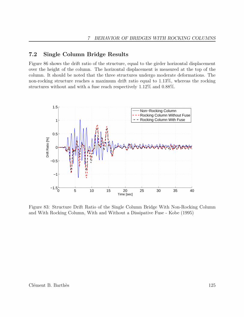
7 BEHAVIOR OF BRIDGES WITH ROCKING COLUMNS
7.2 Single Column Bridge ResultsFigure 86 shows the drift ratio of the structure, equal to the girder horizontal displacementover the height of the column. The horizontal displacement is measured at the top of thecolumn. It should be noted that the three structures undergo moderate deformations. Thenon-rocking structure reaches a maximum drift ratio equal to 1.13%, whereas the rockingstructures without and with a fuse reach respectively 1.12% and 0.88%.
0 5 10 15 20 25 30 35 40−1.5
−1
−0.5
0
0.5
1
1.5
Time [sec]
Drif
t Rat
io [%
]
Non−Rocking ColumnRocking Column Without FuseRocking Column With Fuse
Figure 83: Structure Drift Ratio of the Single Column Bridge With Non-Rocking Columnand With Rocking Column, With and Without a Dissipative Fuse - Kobe (1995)
Clément B. Barthès 125

7 BEHAVIOR OF BRIDGES WITH ROCKING COLUMNS
Figure 84 shows the moment-curvature response for the non-rocking bridge. As expected,the column yielded at both ends of the column. Due to the flexural flexibility of the girder,the moment is larger at the base of the column. The maximum ductility ratio observed is4. Therefore, the bridge resisted the earthquake, but the column is damaged. Conversely,the rocking columns remained elastic. Figure 85 shows the resisting moment observed atthe column joints during the earthquake excitation. The column’s resisting moment of thetwo structures allowed to rock (with and without the fuse) is 86% lower than the resistingmoment of the non-rocking column. It should also be noted that the fuse does not changethe resisting moment significantly.
−5 −4 −3 −2 −1 0 1 2 3 4 5
x 10−3
−1.5
−1
−0.5
0
0.5
1
1.5x 10
5 Bottom
Curvature [rad/m]
Res
istin
g M
omen
t [kN
⋅m]
−5 −4 −3 −2 −1 0 1 2 3 4 5
x 10−3
−1.5
−1
−0.5
0
0.5
1
1.5x 10
5 Top
Curvature [rad/m]
Res
istin
g M
omen
t [kN
⋅m]
Figure 84: Moment-Curvature at the Column Joints for the Single Column Non-RockingBridge - Kobe (1995)
Clément B. Barthès 126

7 BEHAVIOR OF BRIDGES WITH ROCKING COLUMNS
0 2 4 6 8 10 12 14 16 18 20−1.5
−1
−0.5
0
0.5
1
1.5x 10
5 Bottom
Time [sec]
Mom
ent [
kN⋅m
]
0 2 4 6 8 10 12 14 16 18 20−1.5
−1
−0.5
0
0.5
1
1.5x 10
5 Top
Mom
ent [
kN⋅m
]
Non−Rocking ColumnRocking Column Without FuseRocking Column With Fuse
Figure 85: Resisting Moments at Column Joints of the Single Column Bridge With Non-Rocking Column and With Rocking Column, With and Without a Dissipative Fuse - Kobe(1995)
Clément B. Barthès 127

7 BEHAVIOR OF BRIDGES WITH ROCKING COLUMNS
Figure 86 shows the rocking rotations at the column joints with and without a fuse. Itis normalized with respect to the slenderness angle of the column α = 0.0624rad. At bothends, the rocking rotations remain moderate. It is considered that the rocking remains stableonly when θrocking < α however, in this example, the cable may fail for θrocking > 0.8α.
0 2 4 6 8 10 12 14 16 18 20−0.2
−0.1
0
0.1
0.2Bottom
Time [sec]
θ/α
0 2 4 6 8 10 12 14 16 18 20−0.2
−0.1
0
0.1
0.2Top
θ/α
Without FuseWith Fuse
Figure 86: Rocking Rotations at Column Joints of the Single Column Bridge, With andWithout a Dissipative Fuse - Kobe (1995)
In this example, the resisting moment was significantly reduced as shown in Figure 85and the rocking rotation was limited. Hence the rocking column combined with a restrainingcable proved to be a good solution to preserve stability during a large earthquake. The fuseslightly reduces the rocking rotation, but it is not essential since the drift ratio is alreadymoderate when no fuse is used. The energy dissipation of the fuse increases with the rockingrotation. Thus, it is expected to reduce the drift ratio significantly if the rocking rotationbecomes important, as shown in the example presented in Section 7.3.
Clément B. Barthès 128

7 BEHAVIOR OF BRIDGES WITH ROCKING COLUMNS
The stress and the plastic strain in the fuse are shown in Figure 87. A fuse with almostno hardening was intentionally chosen to avoid residual drift (as explained in 6.4). As aconsequence, the maximum plastic strain is 1.2% but there is almost no residual plasticstrain inside the fuse at the end of the excitation. The weight of the structure is sufficientto reduce the plastic elongation and to recenter the column.
0 5 10 15 20 25 30 35 400
0.5
1
1.5
Fus
e P
last
ic S
trai
n [%
]
0 5 10 15 20 25 30 35 40−400
−200
0
200
400
Time [sec]
Fus
e S
tres
s [M
Pa]
Figure 87: Fuse’s Stress and Plastic Strain of the Single Column Bridge - Kobe (1995)
Clément B. Barthès 129

7 BEHAVIOR OF BRIDGES WITH ROCKING COLUMNS
Figure 88 shows the stress in the restraining cable during the earthquake excitation. De-spite significant increase when the column is rotating, the cable is far from exceeding itsfailure strength fu = 1, 800MP a. It was shown in Chapter 6 that cable failure must beavoided to preserve the stability of the structure. In this example, the PT cable behaves asintended. It was designed to resist rocking rotation up to 0.8α, but the maximum rockingrotation observed is only 0.18α.
0 5 10 15 20 25 30 35 400
100
200
300
400
500
600
700
800
Time [sec]
Cab
le S
tres
s [M
Pa]
Without FuseWith Fuse
Figure 88: Restraining Cable Stress of the Single Column Bridge, With and Without Fuse -Kobe (1995)
Clément B. Barthès 130

7 BEHAVIOR OF BRIDGES WITH ROCKING COLUMNS
Finally, it is proposed to study the shear demand on the foundation between the con-ventional bridge and the two bridges equipped with rocking columns (with and without afuse). Figure 89 shows the horizontal reaction force at the base of the column during theearthquake excitation. The shear force is 82% less when the column is allowed to rock. Thisresult is consistent with the reduction of the resisting moment observed in Figure 85, showinga reduction of 86%.
0 2 4 6 8 10 12 14 16 18 20−15,000
−10,000
−5,000
0
5,000
10,000
15,000
Time [sec]
She
ar R
eact
ion
For
ce [k
N]
Non−Rocking ColumnRocking Column Without FuseRocking Column With Fuse
Figure 89: Shear Demand on the Footing of the Single Column Bridge - Kobe (1995)
The demand on the foundation is greatly reduced when the column is allowed to rock.This finding may help to reduce the cost of the foundation. For instance, the number ofpilings can be reduced and the footing can be smaller.
Clément B. Barthès 131

7 BEHAVIOR OF BRIDGES WITH ROCKING COLUMNS
7.3 Two-Columns BridgeColumns of different heights were selected to investigate how rocking would be affected.Columns of the same height are expected to rock together however, columns of differentheights may not do so. A tall column will overturn with a smaller rotation than a shortcolumn and initiation of rocking may be different since they have a different aspect ratio.But the girder is expected to force both columns to rock together. A complex interactionbetween the two columns will govern the rocking behavior of the structure.
The structure’s drift ratio is presented in Figure 90. Note that it is computed consideringthat the height of the structure is the height of the short column and not the height of thetall column. The bridge with non-rocking columns has a maximum drift ratio of only 0.7%,whereas the bridge with rocking columns and without fuses has a maximum drift ratio of2.5%. However, the bridge allowed to rock but equipped with fuses has a maximum driftratio of only 0.75%. Thus, in this example, the fuse significantly helps to reduce drift.
Clément B. Barthès 132

7 BEHAVIOR OF BRIDGES WITH ROCKING COLUMNS
0 2 4 6 8 10 12 14 16 18 20−3
−2
−1
0
1
2
3
Time [sec]
Drif
t Rat
io [%
]
Non−Rocking ColumnsRocking Columns Without FuseRocking Columns With Fuse
Figure 90: Structure Drift Ratio of the Two-Columns Bridge With Non-Rocking Columnsand With Rocking Columns, With and Without a Dissipative Fuse - Kobe (1995)
Clément B. Barthès 133

7 BEHAVIOR OF BRIDGES WITH ROCKING COLUMNS
−5 −2.5 0 2.5 5
x 10−3
−1.5
−1
−0.5
0
0.5
1
1.5x 10
5 Tall Column − Bottom
Curvature [rad/m]
Res
istin
g M
omen
t [kN
⋅m]
−5 −2.5 0 2.5 5
x 10−3
−1.5
−1
−0.5
0
0.5
1
1.5x 10
5 Tall Column − Top
Curvature [rad/m]
Res
istin
g M
omen
t [kN
⋅m]
−5 −2.5 0 2.5 5
x 10−3
−1.5
−1
−0.5
0
0.5
1
1.5x 10
5 Short Column − Bottom
Curvature [rad/m]
Res
istin
g M
omen
t [kN
⋅m]
−5 −2.5 0 2.5 5
x 10−3
−1.5
−1
−0.5
0
0.5
1
1.5x 10
5 Short Column − Top
Curvature [rad/m]
Res
istin
g M
omen
t [kN
⋅m]
Figure 91: Moment-Curvature at the Column Joints for the Two-Column Non-RockingBridge - Kobe (1995)
Figure 91 shows the moment-curvature response at each column joint of the non-rockingbridge. In this example, only the short column yields, only at the base. In the previoussection, it was already observed that the resisting moment was larger at the base, due tothe flexural flexibility of the girder. In this example, it is more noticable since the column isshorter and the girder did not change. Furthermore, the short column is much stiffer thanthe tall column. Therefore, the drift ratio of the tall column remains low and the columndoes not yield.
The maximum ductility ratio observed is 2.6. Therefore, the bridge resisted the earth-quake but the short column is damaged. Conversely, the rocking columns remained elastic.Figure 92 shows the resisting moment observed at each column joint during the earthquakeexcitation. Only the first 20sec are represented. The resisting moment at the ends of therocking columns is significantly lower than the resisting moment at the ends of the non-rocking columns. At the base, the resisting moment is 72% lower for the tall column and85% lower for the short column.
Clément B. Barthès 134
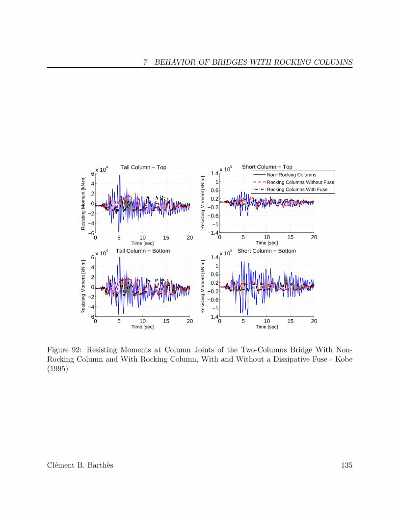
7 BEHAVIOR OF BRIDGES WITH ROCKING COLUMNS
0 5 10 15 20−6
−4
−2
0
2
4
6x 10
4 Tall Column − Top
Time [sec]
Res
istin
g M
omen
t [kN
⋅m]
0 5 10 15 20−1.4
−1
−0.6
−0.2
0.2
0.6
1
1.4x 10
5 Short Column − Bottom
Time [sec]
Res
istin
g M
omen
t [kN
⋅m]
0 5 10 15 20−1.4
−1
−0.6
−0.2
0.2
0.6
1
1.4x 10
5 Short Column − Top
Time [sec]
Res
istin
g M
omen
t [kN
⋅m]
0 5 10 15 20−6
−4
−2
0
2
4
6x 10
4 Tall Column − Bottom
Time [sec]
Res
istin
g M
omen
t [kN
⋅m]
Non−Rocking Columns
Rocking Columns Without Fuse
Rocking Columns With Fuse
Figure 92: Resisting Moments at Column Joints of the Two-Columns Bridge With Non-Rocking Column and With Rocking Column, With and Without a Dissipative Fuse - Kobe(1995)
Clément B. Barthès 135

7 BEHAVIOR OF BRIDGES WITH ROCKING COLUMNS
Figure 93 shows the rocking rotations at each rocking surface. Each rotation plot isnormalized with the slenderness angle of the concerned column. Hence the two columnsslenderness ratios must be distinguished they are αtall = 0.0624rad and αshort = 0.124rad.In this example, the fuses significantly reduce the rocking rotations. In fact, the maximumrocking rotations at the base of the tall column and the short column are respectively 74%and 71% smaller when fuses are used.
0 5 10 15 20−0.2
−0.1
0
0.1
0.2Tall Column − Botom
Time [sec]
θ/α ta
ll
0 5 10 15 20−0.2
−0.1
0
0.1
0.2Tall Column − Top
Time [sec]
θ/α ta
ll
0 5 10 15 20−0.2
−0.1
0
0.1
0.2Short Column − Top
Time [sec]
θ/α sh
ort
0 5 10 15 20−0.2
−0.1
0
0.1
0.2Short Column − Bottom
Time [sec]
θ/α sh
ort
Without FuseWith Fuse
Figure 93: Rocking Rotations at Column Joints of the Two-Columns Bridge, With andWithout a Dissipative Fuse - Kobe (1995)
Clément B. Barthès 136

7 BEHAVIOR OF BRIDGES WITH ROCKING COLUMNS
The stress and the plastic strain in the fuses are presented in Figure 94. A fuse withalmost no hardening was intentionally chosen to avoid residual drift. The maximum plasticstrains are 0.35% and 0.9% but, due to the gravity load, there is almost no residual plasticstrain inside the fuses at the end of the excitation. Thus, the weight of the bridge is sufficientto recenter the column.
0 5 10 15 200
0.4
0.8
1.2
Fus
e P
last
ic S
trai
n [%
]
0 5 10 15 20−400
−200
0
200
400
Time [sec]
Fus
e S
tres
s [M
Pa]
Fuse of the Tall ColumnFuse of the Short Column
Figure 94: Fuse’s Stress and Plastic Strain of the Two-Columns Bridge - Kobe (1995)
Clément B. Barthès 137

7 BEHAVIOR OF BRIDGES WITH ROCKING COLUMNS
The horizontal reaction forces at the base of each column are represented in Figure 95.When the columns are allowed to rock, the shear reaction at the base of each column is73% lower. This result is consistent with the reduction of the resisting moments observed inFigure 92 when the columns are allowed to rock. As observed in the pervious section, theuse of a fuse does not change the reaction force significantly.
0 2 4 6 8 10 12 14 16 18 20−6,000
−4,000
−2,000
0
2,000
4,000
6,000Tall Column
She
ar R
eact
ion
For
ce [k
N]
0 2 4 6 8 10 12 14 16 18 20−18,000
−12,000
−6,000
0
6,000
12,000
18,000Short Column
Time [sec]
She
ar R
eact
ion
For
ce [k
N]
Non−Rocking ColumnsRocking Columns Without FuseRocking Columns With Fuse
Figure 95: Shear Demand on the Footings of the Two-Columns Bridge - Kobe (1995)
Clément B. Barthès 138
7 BEHAVIOR OF BRIDGES WITH ROCKING COLUMNS
7.4 ConclusionIn this chapter, the rocking element was used to assess the performance of an entire bridgestructure when the columns are allowed to rock. It was chosen to compare the results withconventional monolithic bridges. Such bridges in current design philosophy can undergosignificant damage at the column joints during an earthquake. Hence, in order to properlyrepresent the permanent deformations of the columns, it was decided to use a fiber elementwith hysteretic models for the concrete and the longitudinal steel reinforcements.
The same bridges were allowed to rock with a restraining cable preventing overturn-ing. The results showed that the rocking rotations remained moderate if the columns wereequipped with a dissipative fuse. The bridges allowed to rock had a drift ratio of the samemagnitude as the monolithic bridges that suffered from plastic hinge formation. The lim-itation of the rocking rotations within a controlled range was also crucial to preserve theintegrity of the restraining cables. In fact, as the rocking rotations increase, the resistingforces within the cables also increase and it was shown in Chapter 6 that cable failure mustbe avoided.
The resisting moments at the joints of the columns were significantly reduced when thecolumns were allowed to rock. As a result, none of the rocking column was damaged afterthe earthquake. Furthermore, there was no residual drift even when fuses were used. The re-duction of the resisting moment was the primary reason to study the use of rocking columnsand the solution presented in this chapter proved to be very effective. It also shows thatthe capacity of the girder and the column footings can be reduced as shown in Figure 89and Figure 95. In order to transfer the moment loads from the column to the girder, thebent caps are often massive in conventional earthquake resistant bridges. The use of rockingsurfaces may allow to reduce their capacity. The capacity of the columns footings is alsoa very challenging problem. In fact, when the moment at the base of the column is verylarge, the foundation may be in tension. Hence it requires the use of deep concrete pilingsto ensure the stability of the footing. Therefore, the use of rocking columns may allow toreduce the size of the pilings and speed up the construction.
In the first example, the fuse at the base of the column was not affecting the responsesignificantly because the rocking rotation remained low even without a fuse but, in the sec-ond example, the rocking rotations were greatly reduced when fuses were used at the baseof each column. Such device can prevent large rocking rotations and enhance the overallstability.
Clément B. Barthès 139

8 SUMMARY AND CONCLUSIONS
8 Summary and Conclusions
8.1 SummaryCurrent philosophy in bridge earthquake engineering is to ensure the continuity between thedifferent parts of the structure. The columns are designed to yield and form zones (plastichinges) where plastic deformation is expected to occur while keeping the developed resistingforces capped and under control. The remaining bridge elements are then capacity-designedto remain elastic under the forces capped by those that can be developed in the columnplastic hinges.
The goal of this research is to develop a design approach that allows for a substantial re-duction in the forces transmitted from the columns to the bridge elements while keeping thedeformations (both maximum and residual) to the same or smaller level as the convention-ally designed bridge. The design method to achieve this goal is to use segmented columns,comprised of stacked segments with dry or grouted joints post-tensioned using a cable alongthe longitudinal column axis. This design method enables a broad advance of acceleratedbridge construction principles to regions where seismic loads are significant. This design mayallow rocking motion between the segments but also between the column and the foundation,and between the column and the bent-cap. Implementation of this approach in modular andaccelerated bridge construction was presented in Chapter 2. It is expected that modulardesigns with rocking rather than monolithic joints will greatly increase construction speed,have an earthquake performance equal to or better than conventional monolithic designs,and have significantly better repairability characteristics achieved through replacement ofdamaged elements rather than conventional repair and retrofit.
It is sometimes necessary to eliminate rocking at segment interfaces. For instance if rock-ing occurs at column’s mid-height, the off-centered gravity load of the superstructure willcause buckling and lead to collapse. However, rocking can also be used to modify the seismicresponse of bridge structures. The mechanics and dynamics basis for this approach was pre-sented in Chapter 3. Despite its inherent instability, it was shown that rocking behavior maybe a very efficient seismic response modification mechanism for slender structures. Whiledisplacements of the rocking systems are large, the forces transmitted from the rocking el-ements to the rest of the structure are small. It was shown that post-tensioning greatlyreduces the moments in the columns and the demands on the foundation. Despite negligibleenergy dissipation at the rocking surface, the motion of the rocking system was shown toattenuate and eventually disappear.
The rocking element presented in Chapter 4 is essential for modeling complex rocking
Clément B. Barthès 140
8 SUMMARY AND CONCLUSIONS
systems where rocking may occur simultaneously at several rocking surfaces, namely, be-tween the columns and the footings, but also between the columns and the superstructure.If rocking must be prevented between two segments, the rocking element can also be usedto confirm that rocking will not be triggered during the duration of the earthquake. Therocking surface finite element was developed using the augmented Lagrangian formulation,combined with an HHT integration scheme. The element behavior was verified against ana-lytical solutions for free rocking.
The behavior of elastic rocking columns was investigated in Chapter 5. It was shownthat the free rocking response of an elastic column is very similar to the response of a rigidblock. However, the rocking rotations of an elastic column may suddenly stop and lead tobending oscillations.
For a very large earthquake, a column’s rocking can lead to the failure of the restrainingcable. It was shown in Chapter 6 that such scenario must be avoided. The cable has toremain elastic in order to preserve the initial prestressing force and prevent overturning.
At last, a model of a rocking bridge featuring the rocking element was used in Chapter7 to investigate longitudinal direction rocking of a three-span bridge with different columnlengths (i.e. aspect ratios). The element enabled computation of rocking response to anearthquake ground motion.
8.2 ConclusionsIn Chapter 3, the behavior of a rigid block rocking on its base was studied. Previous stud-ies showed that when a block is allowed to rock under earthquake excitation, the resistingmoment at the base of the structure may be greatly reduced, but overturning may occur.So it was proposed to use an unbonded post-tensioning cable, in order to allow rocking butprevent overturning. This solution proved to be very effective. Actually, by adding an elasticcable, a rocking block system can be stable. Furthermore, by changing the cable’s initialprestressing force, it is possible to adjust the minimum ground acceleration required to trig-ger rocking. However, it was shown that the cable elongation can be very large, especiallyfor squat blocks. Hence the cable may fail.
The main purpose of the research presented in this thesis is to apply the findings made oncable restrained rocking blocks to earthquake resistant bridge design. Hence the interactionbetween the material deformations of the bridge and the rotations of the rocking surfaces
Clément B. Barthès 141
8 SUMMARY AND CONCLUSIONS
has to be modeled. But current literature focuses on the rocking behavior of rigid blocks,making it impossible to represent the behavior of a large deformable structure combined withrocking surfaces. Hence it was proposed to use a completely different approach; implement azero-length rocking element. The implementation of this element was described in Chapter4. It was shown that this element combined with a stiff beam element can match the resultsobtained with the rigid block model. This rocking element was essential to demonstrate thefindings made in Chapters 5, 6 and 7.
This element allowed to compute the behavior of a rocking bridge structure under earth-quake excitation. It helped to confirm that moderate rocking can be very beneficial. Ac-tually, compared to a conventional monolithic structure, the base moment of the structurewas greatly reduced whereas the drift ratio remained moderate. It allowed to reduce thecapacity of the column’s footings as well as the bent cap.
Several column configurations were investigated in Chapter 6. It was shown that when aplastic hinge forms at the base of the column, the rocking rotations are greatly reduced dueto the energy dissipation. But such finding does not apply to a real structure. If a plastichinge forms at the base of the column, it will necessarily affect the behavior of the rockingsurface and compromise the integrity of the structure. Chapter 6 also revealed that cablefailure can lead to overturning, hence design criteria must prevent such scenario. It was pro-posed to replace the cable with a tie-rod. This rod was able to yield moderately. However,it was shown that as soon as the tie-rod yielded the initial prestressing force dropped andthe structure became unstable. Hence, it was concluded that the cable must remain elastic,even during a severe earthquake.
It was also proposed to use a mild-steel dissipative fuse to bound the rocking columnwith its footing. It allowed a cantilever column to resist a large earthquake with small rock-ing rotation. It was shown that if the capacity of the fuse is too high, it may prevent thecolumn to return to its initial position. Furthermore, once the fuse yielded it may act asa spring against the weight of the structure and cause rocking to occur even for a minorground motion. However, if the fuse is designed properly, it can help to reduce the rockingrotations and enhance the stability of the structure.
8.3 Recommendations for further researchFuture work on the rocking column bridge concept should focus on the following importantproblems:
Clément B. Barthès 142
8 SUMMARY AND CONCLUSIONS
• Development of a 3D rocking element
• Design of the rocking surfaces
• Model the damaged rocking surface within the rocking element
• Design of rocking bridge prototypes
The rocking element presented in chapter 4 is moving in plane. The kinematic equationsare significantly more complex in three dimensions [33]. In addition different shapes for therocking surface may generate extremely different behaviors. If the rocking surface is circular,the column will no longer rock but it will roll. This phenomenon is shown in [33], for instancea soda can tilted on its side will roll on its edge, even though it seems to rock. The sign of therotation is not determined, it will roll one way or the other depending on the perturbationapplied to the support. A finite element model that intends to describe the rocking/rollingkinematics of a circular surface needs to detect these bifurcation points. Furthermore, asystem analysis may involve different scenarios; for instance if two bridge columns roll, thebridge may behave very differently whether they roll in the same or in the opposite direction.
Since circular surfaces do not rock, they do not dissipate energy. Thus, a rectangularsurface may be more suitable for rocking surfaces in a three dimensional space. But as shownin [34] rectangular surfaces may lead to instability. Namely, when a column tilts in both xand y directions, it may rotate on the corner of its rectangular base.
Development of a rocking/rolling three dimensional finite element is crucial to under-standing the behavior of complex rocking structures with arbitrary rocking surfaces. Inorder to develop design guidelines, the complex instability behavior of such columns must beunderstood. Polygonal shape rocking surfaces with round corners may be able to rock/rollwithout becoming unstable. Such surfaces have not been studied yet, and further researchshould explain in detail their complex behavior.
Rocking surfaces are subjected to large and numerous impacts. Hence design guidelinesmust also pay attention to the rocking surface details. If the surface remains elastic, theshock wave will radiate and dissipate through the column. If the rocking surface undergoespermanent deformations, it may dissipate all the energy that the shock wave may propagate.So ideally a rocking surface should dissipate most of the energy induced by the shock wave,but it must withstand the gravity load during and after the earthquake excitation. Moreover,the rocking surface has to keep its sharp geometry, or the rocking kinematics may changeand become unstable. Actually, if the edges of the rocking surface are damaged, the column
Clément B. Barthès 143
8 SUMMARY AND CONCLUSIONS
may roll on its foot instead of impacting from one corner to the other.
These design characteristics are very similar to ballistic shielding design requirements.Large bullet impacts are dissipated through multiple crack propagation: a matrix bondsthe composite material in order to resist multiple impacts. Hence, bullet-proof windows aredesigned such that the crack length is maximized during impact, and an adhesive layer holdsit in place such that during a second impact the crack will close and lead to new cracks.The use of fiber reinforced concrete may have these properties. The high strength concretecan dissipate energy through crack propagation, and the fibers should be able to hold thecracked elements together. A steel jacketing may help to confine the whole surface and addstrength. A prefabricated rocking surface element could be inserted in the formwork whilemore conventional concrete is cast.The dissipation observed in this thesis is a lower bound. It is expected to be higher with ahighly dissipative rocking surface as shown by ElGawady et al. [9].
As the rocking surface is damaged, its behavior will change. The edges of the rockingsurface will loose their sharpness and the rocking radius may decrease because the impactwill primarily affect the edges. It is crucial to model this localized damage because it maylead to instability, if the overturning occurs at demands smaller than predicted using a dam-ageless model.
Rocking surface damage could be modeled as a reduction of the radius of the rockingsurface. Such model shall be calibrated using a three dimensional finite element method.But it may be preferred to design the rocking surface such that the radius is not alteredduring a large earthquake. For instance it can be designed to resist a compressive load largerthan the column capacity. Such severe criterion may be satisfied using a high strength fiberreinforced concrete and steel jacketing.
The element presented in this dissertation is unable to represent sliding. It is assumedthat the friction at the base of the column is sufficient to prevent sliding from occuring. Butthe friction coefficient of the rocking surface is very hard to determine. When the column isnot rocking, the contact with the footing is distributed over the entire surface, but when thecolumn is rocking the contact with the footing is localized at one corner. Hence it may bepreferred to design shear connectors such that no sliding can occur at the rocking interface,regardless of the friction coefficient.
Once the rocking columns are properly modeled and understood, a bridge prototype withrocking columns can be designed. It should also meet the new design solutions developed
Clément B. Barthès 144

8 SUMMARY AND CONCLUSIONS
for the next-generation of highwway bridges. Namely, the bridge prototype should be builtwith prefabricated modules and its behavior should be compared to that of conventionallydesigned bridges. A similar approach to the one developed by Dr. Ketchum for the PEERTransportation Systems Research Program can be used. The initial construction costs canbe computed, taking into account the significantly reduced foundation size and number ofpiles needed for rocking columns. A seismic performance study can then be conducted usingthe PEER methodology following the pattern established in [2] to compute the likely repaircosts and repair times for rocking bridges. Then a comparison between conventional androcking bridge seismic performance of comparable bridge structures can be made to investi-gate and quantify the potential benefits of rocking bridges.
Clément B. Barthès 145

BIBLIOGRAPHY
Bibliography[1] East-bay bridge project http://baybridgeinfo.org/.
[2] Ady Aviram, Bozidar Stojadinovic, Gustavo J. Parra-Montesinos, and Kevin R. Mackie.Structural response and cost characterization of bridge construction using seismic per-formance enhancement strategies. PEER report, 2010/01, March 2010.
[3] CalTrans. Seismic design criteria 1.6, November 2010.
[4] Y. H. Chen, W.H. Liao, C.L. Lee, and Y.P. Wang. Seismic isolation of viaduct piersby means of a rocking mechanism. Earthquake Engineering and Structural Dynamics,35:713–736, 2006.
[5] Anil K. Chopra. Dynamics of Structures - Theory and Applications to EarthquakeEngineering. EERI.
[6] M. A. Crisfield. Non-linear finite element analysis of solids and structures. John Wileyand Sons Ltd, 1, 1991.
[7] DSI. Dywidag post-tensioning systems catalogue, April 2006.
[8] M.R. Eatherton, J.F. Hajjar, G.G. Deierlein, H. Krawinkler, S. Billington, and X. Ma.Controlled rocking of steel-framed buildings with replaceable energy-dissipating fuses.14th World Conference of Earthquake Engineering, October 2008.
[9] Mohamed A. ElGawady, Quincy Ma, John W. Butterworth, and Jason Ingham. Effectsof interface material on the performance of free rocking blocks. Earthquake Engineeringand Structural Dynamics, 40:375–392, August 2011.
[10] FEMA. Prestandard and commentary for the seismic rehabilitations of buildings. ASCE,356, 2000.
[11] F. C. Filippou. Fedeaslab http://fedeaslab.berkeley.edu/, 2004.
[12] S. Gajan and B. L. Kutter. Effects of moment-to-shear ratio on combined cyclic load-displacement behavior of shallow foundations from centrifuge experiments. Journalof Geotechnical and Geoenvironmental Engineering (ASCE), 135(8):1044–1055, August2009.
[13] M. Garlock and J. Li. Steel self-centering moment frames with collector beam floordiaphragms. Journal of Constructional Steel Research, 64(5):526–538, 2008.
Clément B. Barthès 146
BIBLIOGRAPHY
[14] Hans M. Hilber, Thomas J. R. Hughes, and Robert L. Taylor. Improved numericaldissipation for the time integration algorithms in structural dynamics. Earthquake En-gineering and Structural Dynamics, 5:283–292, 1977.
[15] Reggie Holt. Pbes cost study: Accelerated bridge construction success stories. FHWAreport, 2006.
[16] George W. Housner. The behavior of inverted pendulum structures during earthquakes.Bulletin of the Seismological Society of America, 53(2):403–417, February 1963.
[17] A. Ibrahimbegovic. Non-linear solid mechanics theoretical formulations and finite ele-ment solution methods. Springer- Solid Mechanics and its Applications, 2009.
[18] Mark Ketchum, Vivian Chang, and Thomas Shantz. Influence of design ground motionlevel on highway bridge costs. PEER Report, November 2004.
[19] D. Konstantinidis and N. Makris. Criteria for initiation of slide, rock and slide-rockrigid-body modes. Joint ASME/ASCE/SES Conference on Mechanics and Materials,June 2005.
[20] Wing-Pin Kwan and Sarah Billington. Unbonded posttensioned concrete bridge piers.i: Monotonic and cyclic analyses. Journal of Bridge Engineering, ASCE, 8(2):92–101,March 2003.
[21] Wing-Pin Kwan and Sarah Billington. Unbonded posttensioned concrete bridge piers.ii: Seismic analyses. Journal of Bridge Engineering, ASCE, 8(2):102–111, March 2003.
[22] N. Makris and D. Konstantinidis. The rocking spectrum and the limitations of practicaldesign methodologies. Earthquake Engineering and Structural Dynamics, 32:265–289,2003.
[23] Tipping Mar. Orinda city hall http://www.tippingmar.com.
[24] Eric E. Matsumoto, Michael E. Kreger, Mark C. Waggoner, and Guclu Sumen. Groutedconnection tests in development of precast bent cap system. Transportation ResearchRecord, 1814:55–64, 2003.
[25] A. Neuenhofer and F. C. Filippou. Evaluation of nonlinear frame finite element models.Journal of Structural Engineering, 123(7):958–966, 1997.
[26] R. Park, D. Kent, and R. Sampson. Reinforced concrete members with cyclic loading.Journal of the Structural Division, 98(7):1341–1360, July 1972.
Clément B. Barthès 147

BIBLIOGRAPHY
[27] M.J.N. Priestley, R.J Evison, and A.J. Carr. Seismic isolation of viaduct piers by meansof a rocking mechanism. Bulletin of the New-Zealand National Society for EarthquakeEngineering, 11(3):141–150, 1978.
[28] I. N. Psycharis. Dynamic behavior of rocking two-block assemblies. Earthquake Engi-neering and Structural Dynamics, 19:555–575, 1990.
[29] M. L. Ralls, B. Tang, S. Bhide, B. Brecto, E. Calvert, H. Capers, D. Dorgan, E. Mat-sumoto, C. Napier, W. Nickas, and H. Russell. Prefabricated bridge elements andsystems in japan and europe. FHWA report, 2005.
[30] B. D. Scott, R. Park, and M. J. N. Priestley. Stress-strain behavior of concrete confinedby overlapping hoops at low and high strain rates. ACI Journal, 79(1):13–27, January1982.
[31] L.F. Shampine and S. Thompson. Event location for ordinary differential equations.Computers and Mathematics with Applications, 39:43–54, 2000.
[32] H. Shenton. Criteria for initiation of slide, rock and slide-rock rigid-body modes. Journalof Engineering Mechanics (ASCE), 122(7):690–693, 1996.
[33] M. Srinivasan and A. Ruina. Rocking and rolling: a can that appears to rock mightactually roll. In press, 2008.
[34] T. Tobita and S. Sawada. Rotation response of a rigid body under seismic excitation.Journal of Engineering Mechanics, 132:375–384, April 2008.
[35] M. F. Vassiliou and N. Makris. Analysis of the rocking response of rigid blocks standingfree on a seismically isolated base. Earthquake Engineering and Structural Dynamics,41(177-196), February 2012.
[36] Lloyd M. Wolf and Michael D. Hyzack. Design of precast bent cap to column connec-tions. Concrete Bridge Conference, 2004.
[37] J. Zhang and N. Makris. Rocking response of free-standing blocks under cycloidal pulses.Journal of Engineering Mechanics (ASCE), 127(5):473–483, 2001.
Clément B. Barthès 148