Design and Renegotiation of Debt Covenants

Nicolae Garleanu

Jeffrey Zwiebel∗

This Version: September 2006

Abstract

We analyze the design and renegotiation of covenants in debt contracts as a specific exampleof the contractual assignment of property rights under asymmetric information. In particular,we consider a setting where managers are better informed than the lenders regarding potentialtransfers from debt to equity that are associated with future investments. We show that thissimple adverse-selection problem leads to the allocation of greater ex-ante decision rights to thecreditor (the uninformed party) – i.e., tighter covenants – than would follow under symmetricinformation. This corresponds well with empirical evidence indicating covenants are indeedvery tight upon inception. Strict covenants in turn lead to a bias in ex-post renegotiation, withthe creditor giving up these excessive rights – i.e., covenants are waived. This result contrastswith the conclusion of standard incomplete contracting models of ex-ante hold-up, where theparty with the more important ex-ante investments – presumably management, rather than thecreditors – is granted decision rights.

∗Garleanu: Wharton School, University of Pennsylvania, 3620 Locust Walk, Philadelphia, PA 19104-6367, emailgarleanu@wharton.upenn.edu; Zwiebel: Graduate School of Business, Stanford University, Stanford CA 94305, emailzwiebel@stanford.edu. We are grateful to George Baker, Bernard Black, Patrick Bolton, Philip Bond, Peter DeMarzo,Itay Goldstein, Hayne Leland, Jonathan Levin, Michael Roberts, Neil Stoughton, Steve Tadelis, Ralph Winter, severalanonymous referees, and seminar participants at Carnegie Mellon, Columbia University, DePaul University, DukeUniversity, New York University, Stanford University, the University of British Columbia, UCSD, the University ofUtah, USC, the American Finance Association Meetings, the NBER Conference on Organizations, the EuropeanFinance Association Meetings and the Western Finance Association Meetings, for helpful comments.

In this paper we analyze the design and renegotiation of covenants in debt contracts as a

particular example of the contractual assignment of property rights under asymmetric information.

We start with the presumption that debtholders are less informed than an entrepreneur about

potential future transfers from debt to equity, and explore the implications of this adverse selection

on the design and subsequent renegotiation of debt covenants. Intuitively, we analyze the notion

that debtholders may receive stronger decision rights (in the form of tighter debt covenants) than

under symmetric information, in order to “protect” them from an informational asymmetry, and

the implications this will in turn have for information acquisition and future covenant renegotiation.

Covenants are a common feature of debt contracts, and are generally understood to protect

debtholders against activities that transfer wealth from them to shareholders. Most corporate debt

contracts include covenants that place restrictions on the issuing firm, and thereby effectively serve

to allocate control rights, in certain states of the world. For example, a firm might not be allowed

to issue new debt if net working capital is below a specified level or if an interest coverage ratio

is too low. Common covenant conditions are based on firm net worth, working capital, leverage,

interest coverage, and cash flow; and involve restrictions on issuing debt, paying dividends, and

investing, or impose actions such as the acceleration of debt payments if the specified condition is

binding.1

A striking empirical regularity, however, is less well understood: covenants are remarkably tight.

Chava and Roberts (2005) documents that at the inception of a debt contract, the average covenant

threshold is only about one standard deviation away from the current value of the accounting ratio

in question. As a consequence, 15%-20% (depending on the type of covenant) of outstanding

loans are in violation during a typical quarter, and conditional on violating a covenant, a loan is

delinquent about 40% of the time. Overall, for current-ratio covenants, about 50% of firms and 42%

of loans are delinquent at some point in their lives, while for the less frequently violated net-worth

covenant, about 30% of the loans are delinquent at some time. Furthermore, given such tight initial

covenants, loans often fall into violation very quickly. The median covenant violation occurs at the

end of the first third of the life of the loan, which translates to only one year from the inception of

the loan. One direct implication of this tightness is that covenants are frequently renegotiated, and

when they are the conditions imposed on the firm are routinely relaxed (or waived), and virtually

never strengthened.2 Our analysis yields a simple explanation based on asymmetric information

1See, for example, Smith and Warner (1979), Smith (1993), and Bradley and Roberts (2004).2 In a typical covenant waiver, the debtholder allows the manager to undertake some action prohibited in an

initial covenant or relaxes the covenant that is in breach, in exchange for a higher interest rate and/or new additionalrestrictions. Note that in principle, covenants that are not in violation could also be renegotiated to be strengthened,by prohibiting some previously allowed actions or by tightening the triggering threshold in exchange for a lowerinterest rate. The asymmetry we note in the text is that while the first type of renegotiation (relaxing the covenant)is common, the latter type of renegotiation (strengthening the covenant) is virtually unseen in practice. See, for

1

and costly renegotiation for the observed tightness of covenants and subsequent debt-contract

renegotiation.

Insofar as covenant “tightness” has not received much direct attention in the literature, we

elaborate here on the observation that covenants are surprisingly strict. Covenant tightness can be

understood as a decision regarding the allocation of decision rights, as covenant violations typically

grant debtholders the right to intervene in decisions that they otherwise would not have the right

to intervene in absent the violation. To address how strict one should expect covenants to be, one

must first consider the role covenants play, and the reason they are frequently renegotiated.

Covenants serve to protect lenders from activities that prevent transfers to borrowers. Effi-

ciency considerations, however, dictate that some activities that transfer wealth from debtholders

to shareholders should be permitted, and some should be restricted. For example, the investment

in both good (positive NPV) and bad (negative NPV) new projects are likely to involve a transfer

from pre-existing debtholders to shareholders, by increasing the risk in firm returns.3 It is of course

in the interest of the entrepreneur, as well as the lender, to design a contract that will induce

efficient ex-post investment decisions, insofar as any anticipated transfers will be reflected in the

issue price of the debt. In practice, however, it is typically not feasible to contractually delineate

all future positive NPV projects ex-ante, or for a court to ex-post enforce such a vague contractual

provision. Consequently, covenants are instead conditioned on more easily observable accounting

variables, such as financial ratios, that are likely to be imperfectly correlated with the availability

of good future projects, and are then renegotiated when more information becomes available.

If this ex-post renegotiation was costless and efficient, and if information was symmetric, the

Coase theorem indicates that the strictness of the initial covenants would not matter: renegotiation

would ensure that the efficient decision would always be made ex-post, and the accompanying

transfers necessary to allow this would be offset in the original contract through level of the interest

rate (Coase (1960)). If instead renegotiating was costly, but information was still symmetric, one

would expect to see contracts written to minimize the need for renegotiation by anticipating, as

efficiently as possible, future optimal investment decisions. That is, covenants would not be written

in a manner that induced frequent future violations that were waived upon renegotiation: i.e.,

covenants would be less strict than what is observed. And if we added to this setting the potential

hold-up of ex-ante investments (that is, the friction most commonly presumed in the incomplete

example, Beneish and Press (1993), Sweeney (1994), and Beneish and Press (1995). Technically, Beneish and Press(1993) do find some covenants that are tightened during renegotiation. However, as noted by Smith (1993), this islikely to involve replacing binding covenants with tighter nonbinding covenants on other variables.

3We will take such “asset substitution activity” of Jensen and Meckling (1976) as a canonical case, but any otheractivity that transfers wealths from debtholders to shareholders would serve the same purpose in our model. Thereis a voluminous finance literature that focuses on the size, costs, and consequences of asset substitution and on othermanners of wealth transfer.

2

contracting literature), one would expect covenants to be weaker still. This follows from noting

that decision rights should be allocated in order to minimize distortions in ex-ante investments due

to the potential of future hold-up;4 and ex-ante “effort” by entrepreneurs or managers is likely to be

more important to the success of investment projects than similar “effort” by outside debtholders

(who frequently play a passive role in firm investments). Consequently, it appears rather surprising

that in practice covenants are so strict and consequently so often in violation.

The explanation that our model provides to this observed strictness is neither deep nor com-

plicated. It does, however, highlight what we believe to be an important consideration in the

assignment of decisions rights, both for debt contracts and in other more general settings, that

has generally received little attention to date. In particular, in our setting, lenders receive strong

decision rights as a consequence of asymmetric information. Simply put, if debtholders are less

informed than an entrepreneur about the potential for future transfers, strong decision rights

(through covenants that effectively allow the vetoing of new investments) may “protect” them

from such transfers. Complicating matters, however, is the fact that lenders with strong rights

may also prefer to veto efficient projects as well as inefficient ones, necessitating renegotiation. Our

model is designed to analyze how robust this general notion is in an equilibrium setting where

decision rights in contracts affect inferences and consequently prices (interest rates), and ex-post

renegotiation is possible. While the model in the text is stylized to keep the analysis simple, we

also demonstrate in Appendix A that our results carry through to a far more general setting which

maintains a few basic elements of our model.

These necessary elements are straightforward: First, there is incomplete information ex-ante

about a future decision. In our setting, an entrepreneur needs to raise money from a lender to

undertake a project at time 0. At a future date (time 1), a decision must be made whether to

invest further and expand the project. The efficiency of this time-1 decision depends on the time-1

state of the world, which is not known by either party ex-ante (at time-0), but which is known

by both parties prior to the investment. While the time-1 state of the world is non-contractible

at time-0, the initial contract can allocate the right to make the time-1 decision. Second, there

is an agency conflict. For simplicity we assume that it is always beneficial for entrepreneurs to

invest further at time 1, and it is always detrimental for the lender. Third, there is asymmetric

information regarding the division of surplus under the new investment. In our model, the new

investment will transfer an uncertain quantity x from the lender to the entrepreneur, where the

entrepreneur knows the realization of x, but the lender only learns this realization at a cost. And

fourth, prior to the time-1 investment, the two parties can renegotiate the decision to be made, or,

4See, for example, Klein, Crawford, and Alchian (1978), Grout (1984), Williamson (1985), and Grossman andHart (1986) for the starting point of this very large literature.

3

equivalently, who gets to make this decision.

In this setting, we find that stronger rights (tighter covenants) are granted to the lender in the

initial contract the greater the asymmetric information, the more costly it is for the lender to become

informed, and the less costly it is to renegotiate. Intuitively, lacking information about future

asset substitution, the lender must form inferences about the entrepreneur’s information based

on the contract that is being offered. In equilibrium, the entrepreneur will have to compensate

the lender for the inferred amount of asset substitution activity that will ensue. “Good types”

– i.e., entrepreneurs who do not have as much such activity at their disposal – will prefer to

give strong decision rights to lenders, even though this leads to excessive renegotiation and ex-

post information-acquisition costs, due to the adverse selection problem. Consequently, lenders

on average will be given stronger decision rights than would follow under symmetric information.

Ex-post renegotiation will in turn be biased towards the uninformed party giving up these excessive

rights, thereby yielding asymmetric renegotiation.5

Our setup also allows us to analyze a natural trade-off between early and late acquisition of

information. The early acquisition of information will allow the lender to negotiate the initial con-

tract without an informational disadvantage, which may lead to a more efficient contract. However,

for some states of the world, acquiring this costly information will prove to be unnecessary; if a

state is reached at time 1 where there is no scope for renegotiation, there is no need for the lender

to be informed. Our lenders must trade off this cost and this benefit when choosing whether to

acquire information ex-ante or ex-post.6

Our paper follows the program laid out in the Grossman-Hart-Moore Property Rights literature

in analyzing the optimal assignment of decision rights given contractual incompleteness.7 However,

we depart from most of this large literature by considering the contractual implications of asym-

metric information with costly information acquisition rather than the standard inefficiency of the

hold-up of non-contractible ex-ante actions.8

5Bradley and Roberts (2004) finds that loans are more likely to include covenants when the borrower is small, hashigh growth opportunities, or is highly levered. These results are readily interpretable in our setting to the extentthat asymmetric information about future transfers is greater with such firms. We would argue that all three arelikely: For example, the scope for asset substitution activities or cash diversions is likely to be larger for firms withfewer reporting standards and for growing firms with more investment opportunities. See Malitz (1986) for similarresults. We discuss empirical implications of our model more in Section 4.

6Designing an optimal contract to avoid information costs (i.e. verification costs) in as many states as possible isof course central to the costly state verification framework of Townsend (1979) and Gale and Hellwig (1985). Oursetup differs in that our lender is presumed to be at an ex-ante informational disadvantage and might choose tomitigate this by learning (ex-ante) about future states of the world. Under costly state verification, both parties areequally informed ex-ante, and the contract is designed to try to allow the lender to avoid ex-post verification costs.

7See Grossman and Hart (1986), Hart and Moore (1990), and Hart (1995).8Stole and Zwiebel (2005) has argued that while ex-ante non-contractible investments have received an enormous

amount of attention in the literature, there are other likely manners of contractual incompleteness, yielding newimplications for the allocation of decision rights and ownership that have been relatively unexplored, which meritfurther attention.

4

One notable incomplete contracting paper that does consider the effect of asymmetric informa-

tion in the design of debt covenants is Sridhar and Magee (1997). This paper, however, focuses on

very different aspects affecting the assignment of covenant rights from us; notably, the informative-

ness of contractible variables and the scope for accounting misrepresentations. Furthermore, their

model assumes the asymmetry in renegotiations that we derive as a central result in our analysis;

i.e., they assume that only the lender, and not the owner, can relinquish rights (through unilateral

covenant waivers when it is beneficial for them to do so). 9

Also related is the financial contracting literature that considers the use of financial contracts

to assign control rights across different states of the world. See for example, Zender (1991), Aghion

and Bolton (1992), Dewatripont and Tirole (1994), Berglof and Von Thadden (1994). In our setting,

however, financial contracts cannot distinguish between states of the world, and, rather, renegoti-

ation serves to allocate control rights across states ex-post. Most closely related in this literature

is a recent paper by Dessein which considers the assignment of control rights under asymmetric

information, applied to a contract between an entrepreneur and a venture capitalist. While Dessein

(2005) differs from ours in a number of significant manners: private benefits lead to noncontractible

agency conflicts rather than the future transfers, informational and contracting assumptions dif-

fer, renegotiation is not considered; it also finds that the informed party (the Entrepreneur) gives

up control rights to the uninformed party (the Venture Capitalist) in order to signal congruent

preferences.10

Finally, there is an empirical finance literature speaking to other aspects of debt covenants. For

example, a number of papers consider the price impact of debt covenants; see, for example, Bradley

and Roberts (2004) or Harvey, Lins, and Roper (2004) for some recent results.

While we focus on the interpretation of debt covenants in this paper, our model could be applied

equally well to a number of other contracting settings where asymmetric information regarding

transfers is important. In the conclusion we briefly comment on applications of our model to

home-mortgage contracts, procurement contracts, sports labor contracts and biotechnology joint

ventures.

9Also notable are Spier (1992) and Hermalin (1988), which demonstrate that contractual incompleteness may arisefrom adverse selection. This bears some similarity to our setting where the choice by the informed party of decisionrights signals information about transfers associated with future decisions. However, by assumption, the decisionrights are always contracted on in our setting (i.e., the contract is not incomplete in this dimension). As such, ourfocus is on the effect of asymmetric information on the allocation of such rights and on subsequent informationacquisition, rather than on contractual incompleteness. Huberman and Kahn (1988) notes that costly contractualcontingencies should decrease with the ability to renegotiate contracts.

10In related papers, Kirilenko (2001) shows that an entrepreneur might relinquish control in order to maintain pricenoisiness that supports equilibrium trade, while Harris and Raviv (2005) study control allocation within a firm in asetting in which both the CEO and a manager have relevant information that they can convey partially via cheaptalk.

5

The paper is organized as follows. Section 1 presents our model, Section 2 characterizes its

equilibrium, and Section 3 analyzes properties of this equilibrium and gives intuition. Section 4

highlights some empirical implications, and Section 5 concludes. Further extensions that more

explicitly model several features specific to debt contracts, and proofs, are given in the appendices.

1 The Model

We consider a wealth-constrained entrepreneur E who needs funding I at time 0 to undertake

a project. Ex-ante E faces a competitive lending market and consequently offers a break-even

contract to a lender L in return for I. Both E and L are risk-neutral, and for simplicity, the

discount rate is 0. If undertaken, this project yields a certain return of R at time 2 (provided

that no further investments – described below – are taken). In return for this financing, E signs a

contract {r, D} specifying a promised (deterministic) payment D to L when returns are realized, and

an allocation of the time-1 decision right to one party r ∈ {E, L} (as described below). Note that

we concentrate exclusively on debt contracts and study the optimal allocation of control within this

class of contracts. We do not address the more general security-design question, assuming instead

that debt is chosen for common reasons that we do not model.11

If the parties enter into such an agreement, play proceeds as summarized in the timeline of

Figure 1, which we now describe in detail. Conditional on undertaking the project at time 0, there

is an opportunity to undertake a further investment at time 1. One interpretation is simply an

expansion of the initial project. This further investment requires no additional cash outlay. We

denote the decision to take or not take this additional investment by A (action) and NA (no action),

respectively. The initial time-0 contract specifies who has the right to make this investment decision;

if this right is assigned to L, we will call this a covenant.12 However, the parties may choose to

renegotiate prior to this investment decision. In particular, the party that does not have the decision

11For our purpose, all we need is a contract that introduces an agency conflict between the creditor and thefirm regarding transfers under future actions. Similar implications would follow with alternative contracts with thisfeature. Also, while we speak of an entrepreneur holding equity, we could equivalently speak of a manager acting onbehalf of shareholders.

12 In practice, debt covenants that allow debtholders the right to veto investments are generally contingent on averifiable state of the world; e.g., a low capital ratio. Such contingent covenants would naturally follow in our model,to the extent that new investments primarily transfer wealth from lenders to shareholders only in certain verifiablestates (i.e., when the firm is in or near financial distress). Such contingencies could easily be accounted for, albeit atthe cost of needlessly complicating the model. In particular, consider the following addition to the model: Assumethat there is an additional moment in time – say, time 1

2– between when the initial contract is signed at time 0 and

time 1. Between time 0 and time 1

2, L and E learn whether E is in “financial distress” or not, an event presumed to

be contractible at time 0. If E is not in financial distress, then no asset substitution activities are possible (as debtwill be safe and paid for sure). If E is in financial distress, the game proceeds as in our model, with the same payoffs.In such a setting, the equilibrium time-0 contract would grant the entrepreneur control contingent on there being nofinancial distress at time 1

2, and would follow our equilibrium contingent on financial distress.

6

Contract andinitial investment

Staterevelation Renegotiation

Furtherinvestment

Payoffs

0 1 2

Figure 1: Time diagram

right might pay the other party in order to take a different action (or, equivalently, to transfer the

decision right). We let t represent the net payment from E to L in such a renegotiation.13

For simplicity, we assume that in such renegotiations, L makes a take-it-or-leave-it offer, but

observe here that this assumption does not play an important role in our results. As we discuss

below, for the main case we consider (when L always buys information either at time 0 or time

1), the outcome is independent of the ex-post bargaining division specified here, as the time-0

agreement anticipates this division and adjusts accordingly. We further assume that renegotiation

is costly, in that a fixed cost cr > 0 has to be paid by L, in order to renegotiate. We interpret this

cost as an administrative cost, including, among others, legal expenses and the opportunity cost

of time. The renegotiation cost gives the two parties an incentive to write an initial contract that

minimizes the probability of renegotiating.14

After the time-0 project is undertaken, the state of the world is revealed to be either good (G)

or bad (B) to both parties. An ex-ante contract contingent on the realization of state is assumed to

be impossible. Prior to the revelation of the state, both E and I only know that the probability of

state G is p. The time-1 investment is efficient in state G and inefficient in state B. In particular,

at time 2, this added investment will yield additional expected returns of y > 0 for E and 0 for

L in state G, and additional expected returns of −y for L and 0 for E in state B, where y is

deterministic and known ex-ante by all.15

13We do not allow for contracts that give a party the decision right subject to making a payment to the other partyif the action A is taken. Here we appeal to the standard incomplete contracting justification whereby action A isundescribable ex-ante, perhaps because the nature of future investment opportunities is unknown. Allowing for sucha contract complicates the analysis significantly, insofar as it introduces the possibility of richer signaling. However,there is reason to believe that our qualitative results would still all hold in such a setting.

14Renegotiation costs are assumed to be paid by L only because we have endowed L with all the ex-post bargainingpower, and it is therefore L that realizes all the bilateral gain from such renegotiations. Under an alternativespecification for bargaining power, it would not matter who paid these costs. The case of costless renegotiations(cr = 0) presents some technical complications, but yields a similar equilibrium. Precise results for this case areavailable from the authors on request.

15The assumption that the loss of −y to L in state B is of the same magnitude as the gain y to E in state G

7

Table 1: Game payoffs to (E, L)

A NA Probability

G (R − D + x + y, D − x) (R − D, D) p

B (R − D + x, D − x − y) (R − D, D) 1 − p

Additionally, the time-1 investment will lead to an uncertain transfer x from L to E. This

transfer x can be interpreted as an expected transfer due to increased risk (i.e., asset substitution)

or, alternatively, it can be interpreted as an amount of assets that E can “pocket” for himself due

to the added complexity of further investments. Ex ante, E knows the realization of x, while L

only knows that x is distributed over the interval [a, b], with 0 ≤ a < b, according to the cdf F . For

simplicity we assume that F is atomless with full support over [a, b]. Intuitively, E may know more

than L about future risks involved with a project, or future opportunities to pocket funds.16 We

refer to x as E’s type, and for exposition will adopt the asset-substitution interpretation of x.17

While initially uninformed about x, L can learn its realization for a cost of c0 at time 0 prior

to the signing of the initial contract, or at cost c1 at time 1 prior to the investment decision. We

assume that L’s decision to acquire information is observable to E. We also assume that E cannot

hold up the cost c0 if incurred by L.18

Finally, at time 2, all returns are realized and payoffs are made. We will assume that R is

sufficiently high so that D (which is determined in equilibrium) is less than or equal to R. Table 1

summarizes the Period-2 payoffs to E and L conditional on the state of the world and action.

Several remarks on the payoff matrix are in order here. First, when NA is chosen, the payoffs

are insensitive to both the state (this feature plays no role in the analysis) and, more importantly,

simplifies the notation a little, but it has no impact on the results. This assumption, as well as others (discussed inFootnote 17), is relaxed in Appendix A.

16In principle, transfers from E to L may also be of concern at the contracting stage, but such cases appear farless common or natural, and we do not model them.

17We remark that this interpretation requires uncertain payments after date 2; x and y, therefore, should be viewedas the expectation of these payoffs given the original contract. Consequently, it would be natural for x to depend onthe promised payment D. Similarly, in many settings, the inefficiency −y associated with investing in the bad stateof the world would be divided between E and L as a function of D. (For example, L might suffer the marginal lossof −y only when E was illiquid or when verifiable cash was less than D, with E suffering the loss otherwise.) Forsimplicity we take the reduced-form approach of specifying x and y directly, the realization of x to be independent ofD, and the inefficiency −y to be realized entirely by L, but demonstrate in Appendix A that all qualitative featuresof the model hold when these assumptions are relaxed.

18Otherwise, given our assumption of an ex-ante competitive lending market, L will never expend these time-0costs, as they are sunk, and he will be held to zero profit not including these costs when the contract is signed. Thisassumption can be justified in a number of manners: We could assume that E can commit with L prior to signinga contract to reimburse these costs; or that E could, at a cost c0, make his private information verifiable; or thatundertaking these costs raises L’s outside option by an identical amount (perhaps because the information learnedis equally valuable in alternative relationships). Alternatively, at the cost of some further analysis, we could forgothis assumption altogether by allowing L to have some ex-ante bargaining power. We make this assumption simplybecause we want to explore the trade-off between early and late information acquisition, and our focus is not on thehold-up of ex-ante investment costs.

8

the private information x. In the context of covenants, it is natural to interpret NA as not taking

a further investment; more generally, NA can be interpreted as a “neutral decision” not impacted

by E’s private information. Second, absent renegotiation, L would always prefer NA to A, and E

would prefer A to NA, while the socially optimal choice is A in state G, and NA in state B. This is

of course the essence of our agency problem. Consequently, if E has the decision right, it is efficient

to renegotiate in state B but not state G, and the converse is true if L has the decision right. And

third, we note that the constant R plays no role in the play of the game or in our analysis, save

to ensure that required payments by E are feasible under the interpretation of an ex-ante wealth

constrained entrepreneur. For other interpretations of our model, where E and L have some joint

benefit to cooperation, but where E is not ex-ante wealth constrained, this term is unnecessary.

2 Equilibrium

Before analyzing our model, we first state the outcome for the benchmark setting of symmetric

information. While trivial, it will be informative to compare our results with this benchmark.

Proposition 1 If the two parties are symmetrically informed about x at time 0, then L receives

control rights whenever p < 12 , while E receives control rights whenever p > 1

2 . (The two parties

are indifferent between the two types of contracts when p = 12 .)

This benchmark follows immediately from observing that under symmetric information E simply

offers the break-even contract to L that leads to the least future expected inefficiency (i.e., renego-

tiation costs). When r = L, costly renegotiation is averted in the bad state, whereas when r = E

renegotiation costs are instead averted in the good state. When the bad state is more likely (p < 12)

than the good state, the expected costs are smallest when r = L, and vice-versa. We refer to

this benchmark as the symmetric-information outcome, or the constrained-efficient outcome, since

it minimizes transaction costs, subject to the constraint that contracts cannot be written on the

time-1 state of the world G or B.

Now allowing for asymmetric information, we consider Pure-Strategy Perfect Bayesian Equi-

libria (PSPBE). Since we are primarily interested in the interplay between costly information

acquisition and the assignment of control rights, we will concentrate on parameters such that, in

equilibrium, L acquires information at least in some states. Specifically, we will consider parameters

such that either L acquires information at time 0, or, if L has chosen not to become informed at

time 0, L will choose to become informed at time 1 in states where there is scope for renegotiation.

Proposition 3 in turn will indicate that this holds provided that c1 is small enough. Additionally,

to ensure that ex-post renegotiation ensues when the inefficient action would otherwise be taken,

9

Table 2: Final net payoffs after renegotiation to (E, L)

r = E r = L Probability

G (R − D + x + y, D − x)) (R − D, D + y) p

B (R − D + x, D − x) (R − D, D) 1 − p

we assume that c1 + cr < y. That is, we assume the efficiency gains from renegotiating exceed the

total cost of information acquisition and renegotiation.

We first consider play at time 1, under this presumption that L will become informed by this

time if there is scope for renegotiation. We will define the “state” at this time by a pair (r, s),

where the first element r ∈ (E, L) indicates who possesses the decision right, and the second element

s ∈ (G, B) indicates whether the investment state is good or bad (which is known by both parties

at time 1).19 There are four states to consider. In two of the states, (E, G) and (L, B), there is no

scope for renegotiation, as the owner of the right already prefers the optimal decision. Consequently,

the net payoffs (that is, payoffs including transfers but not including information-acquisition costs)

to E and L are (R−D + x + y, D − x) for (E, G), and (R−D, D) for (L, B). Note that if L is not

informed entering time 1 in one of these two states, there is no need for him to become informed

at this time as such information will yield no benefit. This captures the notion that sometimes

information that is acquired at time 0 is unnecessary.

If instead the state is (L, G) or (E, B), there will be scope for renegotiation. As noted above, we

are presuming for now that at the time of this renegotiation L has become informed and therefore

knows x. In the state (E, B), absent renegotiation, E would choose the inefficient action A, since

that would yield him R − D + x > R − D, despite a combined payoff that is less than that under

action NA, i.e., R − y < R. Given this, L will offer an additional payment x to E in exchange for

action NA to be taken. (Recall that L has all the bargaining power, so L would offer just enough

to keep E indifferent.) Thus, the final net payoffs are (R − D + x, D − x). Similarly, for the state

(L, G), absent renegotiation L would choose NA; thus L will ask for E’s entire marginal benefit

x + y in exchange for taking action A instead. This yields payoffs of (R−D, y + D). The final net

payoffs in the four cases are summarized in Table 2. Note that Table 2 differs from Table 1 only in

that in both inefficient states, renegotiation yields added benefits of y, which are realized entirely

by L since L is assumed to have all of the bargaining power.

Turning to the time-0 contract, note that in any pure strategy equilibrium there can be at most

one contract associated with each choice of the decision right r. That is, if a contract {r, D} is

accepted in equilibrium, no type of E would offer the contract {r, D′}, D′ > D. Consequently,

19We use simple parentheses to designate states to distinguish them from contracts (which are designated withcurly brackets). While we also employ parentheses to denote a pair of payoffs to the two parties, it will be clear fromthe context whether we are referring to states or to payoffs.

10

there are at most two contracts offered in equilibrium, one with r = E and one with r = L. Let

SE ⊆ [a, b] denote the set of types who offer, in equilibrium, a contract with r = E; that is, SE

gives the set of types who keep the decision right.

Now consider the case in which L has not acquired information at time 0, but will acquire

information at time 1 if there is scope for renegotiation. (Later, we shall consider time-0 information

acquisition.) With ex-ante competition between lenders, L must break even for any equilibrium

contract. These contracts of course anticipate correctly that renegotiation will occur in states

(E, B) and (L, G) and not in states (E, G) and (L, B). Given the final payoffs in Table 2, D is

determined by the ex-ante indifference conditions for L. These conditions, for contracts with r = E

and r = L respectively, are

I = D − pE[

x∣

∣ x ∈ SE

]

− (1 − p)(

c + E[

x∣

∣ x ∈ SE

])

(1)

and

I = D + p(y − c), (2)

where c ≡ c1 + cr. With D satisfying these conditions, the final payoffs to E for the contracts with

r = E and r = L, are in turn respectively,

UEr=E = R − I − E

[

x∣

∣ x ∈ SE

]

− (1 − p)c + p(x + y) + (1 − p)x, (3)

and

UEr=L = R − I + py − pc. (4)

Note that E’s payoff increases with x when r = E and is independent of x when r = L.

Consequently, if type x weakly prefers {E, D} to {L, D′}, then all higher types x′ > x would

strictly prefer the former contract. And likewise, if type x weakly prefers {L, D′} to {E, D}, then

all lower types x′ < x would strictly prefer {L, D′}. It follows that in any PSPBE there will be a

cut-off level x (possibly equal to a or b) where all types below x pool together by offering the same

contract with r = L, and all types above x pool on a single contract with r = E. Thus, the set SE

is of the form [x, b].20

To characterize this cut-off level x, it will be quite useful to define the function G(u) as follows:

G(u) ≡ E[

x∣

∣ x ≥ u]

− u. (5)

20Strictly speaking, when interior, type x is of course indifferent, and could choose either contract. Our inclusionof this 0-measure type in the set r = E is inconsequential.

11

Intuitively, G(x) expresses the difference between the average type in the pool [x, b] of all types

above x, and the lowest type x in this pool.

In equilibrium, the cut-off type x must be indifferent between keeping and giving up the right.

Equating expressions (3) and (4) then implies that x is given by:

G(x) = (2p − 1)c. (6)

With this in hand, we now state our main result, which characterizes all PSPBEs. All proofs are

in Appendix B.

Proposition 2 Assume that L pays c1 and learns x at time 1 if there is scope for renegotiation.

Then, a PSPBE always exists, and takes the following form:

(i) If G(x) > (2p − 1)c for all x ∈ [a, b], then all types offer r = L. The promised payment is

D = I − p(y − c).

(ii) If G(x) < (2p − 1)c for all x ∈ [a, b], then all types offer r = E. The promised payment is

D = I + E[x] + (1 − p)c.

(iii) If there exists x ∈ [a, b] such that G(x) = (2p− 1)c, then types x ≥ x offer r = E, while types

x < x offer r = L. The promised payments are: DE = I + E[

x∣

∣ x ≥ x]

+ (1 − p)c when

r = E and DL = I − p(y − c) when r = L.

Note that since F is atomless and G is continuous, the condition for case (iii) will be satisfied

if we are not in case (i) or case (ii), and therefore the three cases form a complete partition of the

space of parameters. We discuss and interpret the equilibrium of Proposition 2 in the next section,

after we first indicate sufficient conditions for its assumptions to be satisfied. Before turning to

these conditions, we illustrate this Proposition with a simple example.

Example 1 Let x be distributed uniformly on [a, b]. Then, G(u) = b−u2 . Note that G(u) is

monotonically decreasing in u. (Proposition 8 below indicates that this will hold whenever the

hazard rate of x is increasing.) Proposition 2 then indicates that:

(i) If p ≤ 12 , then all types of E give the control right to the lender (r = L). (This statement

holds in general, since case (i) of Proposition 2 applies.)

(ii) If p ≥ 12 + b−a

4c, then all types of E retain the control right (r = E).

(iii) If 12 < p < 1

2 + b−a4c

, then x = b− 2(2p− 1)c. E retains the control rights if x ≥ b− 2(2p− 1)c,

otherwise L is granted the control right.

12

0.1 0.2 0.3 0.4 0.5 0.6 0.7 0.8 0.9 1

Probability (p)

Equilibrium x

Type

(x)

probabilit

a

b

0

Figure 2: The figure illustrates the equilibrium cut-off level x below which E gives up the controlrights, for two levels of the cost c. The dashed line corresponds to a lower cost than the solid line.

The allocation of control rights as a function of p in this example is depicted in Figure 2. The solid

line and the dashed line represent two different values of costs c. A cut-off value of b indicates that

none of the types E retain control rights (control rights are always given to L), while a cut-off value

of a indicates that all types E retain control rights. When the cut-off level is in between, types E

above the cut-off retain control, while those below the cut-off give control to L.

For Proposition 2, we assumed that if L is uninformed entering into time 1, he will prefer to

acquire information in states (E, B) and (L, G) – that is, when there is scope for renegotiation.

Proposition 3 indicates that such preferences follow if c1 is small enough. Intuitively, the proof

shows that the losses to L from bargaining with asymmetric information are bounded away from

0, and, consequently, information acquisition is preferred if the cost to this is small enough.

Proposition 3 Assume that L does not acquire information at time 0. Then, there exists c1 > 0

such that, for c1 ≤ c1, L acquires information at time 1 in states (E, B) and (L, G).

We now turn to the case where L acquires information at time 0. As noted above, we assume

that E can commit to reimburse L for this information-acquisition cost c0, or alternatively, can

pay it herself. Thus, information will be acquired at time 0 rather than at time 1 if the ensuing

break-even contract for L yields higher expected profits for E (since lenders compete ex ante with

one another to contract with E). Proposition 4 follows immediately.

Proposition 4 If L learns x at time 0, then

13

(i) if p > 12 , r = E and D = x + I + c0 + (1 − p)cr, and the net profits of E are R − I + py −

c0 − (1 − p)cr;

(ii) if p < 12 , r = L and D = −py + I + c0 +pcr, and the net profits of E are R− I +py− c0−pcr.

When L acquires information at time 0, the total information cost is c0, while the expected

renegotiation cost is the smaller of pcr and (1 − p)cr. Since we are assuming that information

will either be acquired at time 0 or at time 1 if there is scope for renegotiation, the time 1 action

taken will be efficient. Given risk neutrality, it follows that the contract that maximizes E’s utility

subject to the lender breaking even is the contract that minimizes the sum of expected information-

acquisition costs and expected renegotiation costs. Hence, the choice between acquiring information

at time 0 and acquiring it at time 1 follows from simply comparing these costs, as the following

proposition states.

Proposition 5 Assume that c1 is small enough such that L would acquire information at time 1

when there is scope for renegotiation if he had not already done so at time 0. Then, L acquires

information at time 0 if and only if

c0 + min(p, 1 − p)cr ≤ (c1 + cr) [pF (x) + (1 − p)(1 − F (x)] . (7)

Early information acquisition imposes the inefficiency of paying the information cost when it might

not be necessary. More precisely, late information acquisition results in an information-spending

saving of c0 − c1 (pF (x) + (1 − p)(1 − F (x))) compared with early information acquisition. This

saving is always positive provided that c0 ≥ c1 (i.e., provided that the cost of acquiring information

does not increase too significantly over time). On the other hand, early information acquisition

reduces the expected renegotiation costs by minimizing the probability of renegotiating, yielding a

cost saving of cr (max[(1 − 2p), 0] − (1 − 2p)F (x)) . (As we will note in the following Section, this

savings is zero whenever p ≤ 12 , as p ≤ 1

2 implies we are in case (i) of Proposition 2 where the control

right is always assigned in the manner that minimizes renegotiation.) Generally, whether early

information acquisition is preferred to late information acquisition depends on how the additional

information cost compares to the saved renegotiation cost.

Propositions 3 and 5 jointly give conditions under which information will be acquired at time 1 if

there is scope for renegotiation. The former indicates when this will be preferred to no information

acquisition, while the latter indicates when this will be preferred to information acquisition at time

0. In the following section we analyze Proposition 2 under the maintained assumption that these

conditions are satisfied.

14

3 Equilibrium Properties and Discussion

In this section we analyze the properties of our main result, Proposition 2; we derive several

comparative-statics results; we examine the relative frequency of different types of renegotiation;

and we further analyze the decision regarding the timing of information acquisition.

Returning to Proposition 2, the interpretation of the equilibrium condition comparing G(x) and

(2p − 1)c is straightforward. First note that the latter term, (2p − 1)c, measures the additional

renegotiation and information-acquisition costs that must be undertaken when r = L instead of

r = E: this cost is given by pc − (1 − p)c = (2p − 1)c. (The cost is negative if p < 12 , signifying

lower renegotiation costs under r = L than under r = E.)

Turning to G(x), suppose that types [u, b] retain the decision right. (Recall that we previously

showed that in any PSPBE there must be a cut-off level such that types retain the decision right

if and only if they exceed this level.) Then, L would expect asset-substitution activity given by

E[x∣

∣ x ≥ u] when r = E, for which L must be reimbursed ex-ante.21 The lowest type choosing

r = E, type u, would only benefit from asset substitution activity in the amount t. The difference

between these two, E[

x∣

∣ x ≥ u]

− u = G(u), measures the adverse-selection cost faced by this

lowest type u choosing r = E.

In equilibrium, all types must compare the adverse-selection cost from choosing r = E with

the excess renegotiation cost from choosing r = L. The adverse-selection cost is always greatest

for the lowest type choosing r = E, and this is always positive. The excess renegotiation cost, in

contrast, is only positive if p ≥ 12 . When instead p < 1

2 , renegotiation costs are less for r = L

than r = E, and consequently there is no equilibrium with some types choosing r = E; the lowest

type choosing r = E would always benefit by defecting to r = L. Hence, when p < 12 case (i) of

Proposition 2 obtains, all types choosing r = L. This corresponds with the constrained efficient

symmetric information outcome given in Proposition 1.

In contrast, when instead p > 12 , the allocation of the decision right diverges from the constrained

efficient outcome of Proposition 1 if (2p−1)c is not too large. With p > 12 , the constrained efficient

outcome involves all types E retaining the decision right. However, provided that (2p − 1)c does

not exceed GM ≡ maxx G(x), case (iii) obtains in Proposition 2, whereby low types will prefer

to give the decision right to L despite the associated inefficiency in renegotiation and information

acquisition costs. Intuitively, the additional renegotiation and information-acquisition costs that

must be undertaken when r = L instead of r = E is less for some low types than the adverse-

21This follows from noting that, absent renegotiation, E would always choose A if she had the right, and L wouldalways choose NA. Hence, in all states, E requires an added transfer of x if she has the right instead of L. This transferalters threat points, and is maintained through our renegotiation. In contrast, any efficiency gain y is captured entirelyby L in our renegotiation due to our endowing L with the bargaining power through a take-it-or-leave-it offer.

15

0 0.1 0.2 0.3 0.4 0.5 0.6 0.7 0.8 0.9 1

r = Er = L

Probability (p)

Type

(x)

x

Equilibrium

a

b

0 0.1 0.2 0.3 0.4 0.5 0.6 0.7 0.8 0.9 1

Probability (p)

Type

(x)

r = Er = L x

Constrained Efficient

a

b

Figure 3: The figure illustrates the equilibrium allocation of the control rights for all levels ofp when information is asymmetric – left panel – in comparison with the symmetric informationbenchmark case – right panel. The shaded areas represent the types x that relinquish the controlrights.

selection costs they would instead incur by retaining the decision right together with all the high

types who choose to do so. In equilibrium, the lowest type choosing r = E is indifferent: she must

face adverse-selection costs equal to the information and renegotiation-inefficiency costs of instead

choosing r = L; that is, the cut-off type is given by G(x) = (2p − 1)c.

Finally, if (2p − 1)c > GM , then the adverse-selection cost for all types choosing r = E will

always be less than the excess information and renegotiation costs from choosing r = L. In such an

event, case (ii) of Proposition 2 obtains, whereby all types choose r = E. Note that since G(0) > 0,

(2p − 1)c > GM can only occur when p > 12 . When this case occurs, the allocation of the decision

right again matches the constrained efficient outcome of Proposition 1.

Proposition 6 summarizes how the allocation of the control right that follows from Proposition

2 differs from the constrained efficient benchmark of Proposition 1. This comparison is depicted

in Figure 3. In this figure the left panel indicates the control allocation for any value of p under

asymmetric information, whereas the right panel gives the benchmark symmetric information al-

location. Shaded areas represents types of E that give up control of the decision right to L. Note

that with asymmetric information, for any given p, the set of types E that give up this control

right under asymmetric information is a superset of the set of types E that give up this right under

symmetric information.

Proposition 6 Under asymmetric information, when p > 12 and GM > (2p− 1)c, the uninformed

16

party L receives the decision right more frequently than under the constrained efficient symmet-

ric information outcome. When these conditions do not hold, the allocation of the decision right

coincides with the constrained efficient symmetric information outcome.

Comparative-static properties of the equilibrium follow from the behavior of the function G. G

is weakly positive and equals 0 at b. Its maximum value, GM , is at least as large as G(0) = E[x]−a.

G need not, however, be monotonically decreasing, which in general makes the local dependence

of x on parameters such as p or c ambiguous. The following two propositions, however, provide

conditions that ensure this monotonicity. First, Proposition 7 indicates that a necessary and

sufficient condition for G to be monotonically decreasing is that the function G is strictly less than

the inverse hazard rate of x, defined as (1 − F (u))/∂[F (u)]∂u

. The second proposition, Proposition

8, indicates that this condition is always satisfied if x satisfies the standard increasing hazard rate

assumption, which, as is well-known, is satisfied by a large class of common distributions including

the normal, the truncated normal, the exponential, the truncated exponential, and the uniform

distributions, among other distributions.

Proposition 7 Let h denote the hazard of the distribution of x. Then G(x) is strictly decreasing

at x if and only if

G(x) <1

h(x).

Proposition 8 If the hazard rate of the distribution of x is increasing, then G(x) is monotonically

decreasing.

As Proposition 9 below indicates, uniqueness and a number of simple comparative-static prop-

erties of our equilibrium follow from the monotonicity of G. One of the comparative statics we are

interested in is how the contract varies with the amount of asymmetric information. Since changes

in asymmetric information, however, may alter the support of x, we need a measure of asymmetric

information that is invariant to shifts in the support, unlike second-order stochastic dominance. To

this end, we employ the following partial ordering for the dispersion of a distribution.

Definition 1 A distribution F is said to be more dispersed than a distribution F ′ if F−1(q′) −

F−1(q) ≥ F ′−1(q′) − F ′−1(q) whenever 0 < q ≤ q′ < 1.22

22See Shaked and Shanthikumar (1994). Note that our assumptions on the distribution of x imply that F iscontinuous and strictly increasing, which makes F−1 unambiguously defined on [0, 1]. Intuitively, this definition saysthat a distribution with cdf F is more disperse than one with cdf F ′ if for any range of probabilities, the domain ofthe random variable which maps into this range is larger for F than for F ′. Under this definition, a random variableX is less dispersed than Y if and only if Y has the same distribution as X + φ(X) for some increasing functionφ. If the logarithm of the pdf of X is concave, which is the case for the uniform, (truncated) normal, (truncated)exponential, etc., distributions, and which also implies that the hazard rate of X is increasing, then, for any randomvariable Z independent of X, X + Z is more dispersed than X. We also note that the convolution of two randomvariables with increasing hazard rates has an increasing hazard rate, thus ensuring that G remains monotonic.

17

With this definition in hand, we now state several comparative-static results.

Proposition 9 Let p > 12 . If G is strictly decreasing over the range [a, b], then:

(i) x is unique.

(ii) x decreases with both p and c = c1 + cr.

(iii) If F ′ is less disperse than F (i.e., there is less asymmetric information), then F ′(x′) ≤ F (x).

This proposition indicates that the proportion of types who give away the control rights inefficiently

due to asymmetric information is smaller when the renegotiation and information-acquisition cost

c is large, when the probability of the good state p is large, and when the distribution of x is

less disperse. Intuition for these results is straightforward. As noted above, G(x) represents the

adverse-selection costs to x of choosing r = E if he is pooled together with all higher types [x, b]

in choosing E. If G decreases monotonically, then by expanding the interval of types [x, b] that

choose r = E by lowering the cut-off x, the adverse-selection cost to the lowest type x in this pool

increases monotonically as well.23

For any equilibrium where some types E hold control rights and other types do not, the marginal

type must be indifferent to holding control rights and giving them up. If the cost of choosing r = L

increases either by increasing p (making renegotiation more likely) or by increasing c (increasing

the cost of renegotiation), and if G decreases monotonically as well, then it follows that more

types will choose r = E until the adverse-selection cost for the marginal type choosing r = E

increases correspondingly. Consequently, the equilibrium cut-off x falls. Similarly, less dispersion

in asymmetric information implies that the adverse-selection cost for the lowest type in any given

pool choosing r = E decreases. Consequently, more types will join this pool, and x will fall, until

the cost for the marginal type once again equals the cost of inefficient renegotiation. We illustrate

Proposition 9 with the following example.

Example 2 Consider again the uniform distribution of Example 1. As noted in this example,

provided that 12 < p < 1

2 + b−a4c

, the marginal type choosing r = E is given by x = b − 2(2p − 1)c.

(If the condition on p is not met, all types choose the same contract.) Note that, as indicated in

Proposition 9(ii), this cut-off x is clearly decreasing in p and c.

Now suppose that instead x is distributed uniformly over [a − ǫ, b + ǫ], with ǫ > 0. Dispersion

of x increases in ǫ. And provided that p is such that an interior solution obtains, it follows that

23This condition would not, for example, hold at x if there was a mass point at x, in violation of the increasinghazard rate assumption. In particular, lowering the cut-off by a small amount ǫ to include x would lower the meanof the pool by more than ǫ.

18

Cumulative probability (F (x))

Expec

ted

cost

s

(2p − 1)c

(2p − 1)c′

G

G′

0 0.25 0.5 0.75 1

Figure 4: The figure illustrates the equilibria obtaining for two different costs, c′ > c, and for twouniform distributions for x, [a, b] and [a′, b′] with b − a > b′ − a′.

x = b + ǫ − 2(2p − 1)c, and therefore, that F (x) = b−a+2ǫ−2(2p−1)cb−a+2ǫ

, which is increasing in ǫ. Thus,

more asymmetric information increases the proportion of types who choose to relinquish the right

to L even though this is inefficient.

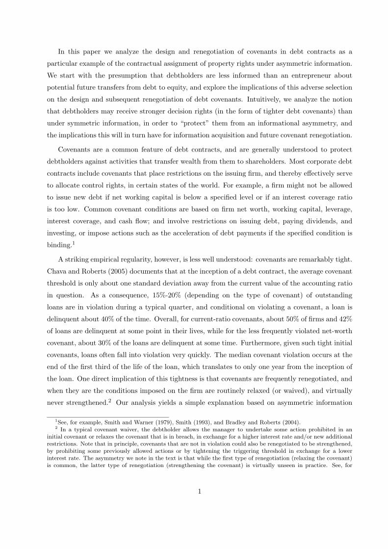
Figure 4 shows the determination of the equilibrium for two different costs, c′ > c, and two

distributions for x, with F more dispersed than F ′. (It is immediate that different probabilities

p′ > p ≥ 12 have the same effect as different costs.) The functions G and G′ correspond to the

two distributions F and F ′ respectively. On the horizontal axis we plot the cumulative probability

F (x) and F ′(x) – since the economically meaningful comparison is not between cut-off levels x, but

between the probabilities F (x) that there is renegotiation in the good state. (For example, shifting

the distribution of x by a constant changes x, but does not change the amount of asymmetric

information, and consequently does not alter F (x) or payoffs in any state.) Adverse selection and

renegotiation costs are plotted on the vertical axis. The adverse-selection cost for the lowest type

choosing r = E, is given by G and G′. If Proposition 8 is satisfied, these costs decrease with the

cut-off x, and, therefore, with F (x) as well. (They are linear here only because of the uniform

distribution chosen in this example). Additional renegotiation costs from choosing r = L rather

than r = E are depicted by the horizontal lines at (2p − 1)c and (2p − 1)c′ for the two different

costs. The equilibrium cut-off type is given by the intersection of this adverse-selection cost and the

additional renegotiation cost. The figure clearly indicates that higher costs and less dispersion in

information lead to lower equilibrium values of F (x), and consequently to less renegotiation.

Proposition 6 indicated that under asymmetric information L obtains the decision right more

19

often than under the constrained efficient outcome at time 0, which in turn implies that L rene-

gotiates to sell the right more frequently than under the constrained efficient outcome at time 1.

Empirically, however, one is likely to only observe absolute magnitudes of renegotiation in each

direction. The following proposition gives conditions under which the frequency of renegotiations

where the uninformed party gives up rights exceeds that where the informed party gives up rights.24

In particular, in our equilibrium, L renegotiates to sell the right with probability ps = pF (x)

if p > 12 and ps = p if p < 1

2 , while L renegotiates to obtain further rights with probability

pb = (1 − p)(1 − F (x)) if p > 12 and pb = 0 if p < 1

2 . When p < 12 , all renegotiation involves

transferring rights from L to E. When instead p > 12 , the following obtains immediately.

Proposition 10 Let p > 12 .

(i) ps > pb if and only if p > 1 − F (x).

(ii) If G is monotonic, the fraction ps

ps+pb of all renegotiations that involve L giving up rights (as

opposed to E giving up rights) decreases with c, and decreases if F becomes less disperse.

(iii) Consider a sequence of economies indexed by n ∈ N characterized by (pn, cn, Fn). The fractionps

n

psn+pb

n

of all renegotiations that involve L giving up rights tends to 1 when either a) pn tends

to 1 and Fn(xn) is bounded away from 0,25 or b) Fn(xn) tends to 1 — in particular, if F and

p are fixed and cn → 0.

If p ≤ 12 , all renegotiations involve L transferring rights for considerations to E. If instead p > 1

2 ,

Proposition 10 indicates that the fraction of renegotiations that involve L instead of E giving

up rights for considerations increases in asymmetric information and decreases in the costs of

24Some have suggested to us, as an alternative explanation for strict covenants, that there is an asymmetry arisingin renegotiations due to the fact that it is “improper” (and at times may be illegal) for shareholders to undertakean inefficient action that transfers wealth from debtholders, and that any renegotiation whereby debtholders makesome other concession to shareholders to prevent such an action would be “unseemly”. This explanation does notstrike us as convincing for several reasons. First, such asset substitution activity is central to shareholder-debtholderagency conflict in finance, and the possibility of such activity is well-acknowledged both in practice and in thefinance literature. Second, it is not clear why such a renegotiation is any more “unseemly” than the converserenegotiation that is often observed in practice, where shareholders make some concession to debtholders in exchangefor debtholders removing their veto over an efficient action. In both cases, the status-quo action that will be takenabsent renegotiation is suboptimal, and for the same reason – the party with the right to make the decision prefersthe suboptimal action. And third, to the extent that a distinction between the two can be made, it is by no meansobvious to us that renegotiations to enhance efficiency are any more prevalent than those to avoid inefficienciesin other settings. For example, legal proceedings in a civil case typically involve costs for both parties involved,whereas a pre-trial settlement of such a case can be viewed as a negotiation designed to avoid the inefficiencies ofsuch proceedings. Consequently, we would instead argue that there is no natural or legal distinction between thesetwo types of renegotiations, and, rather, that assessments of which renegotiations appear “less unseemly” are likely tosimply reflect which type of renegotiation is in fact observed in practice, and therefore, are no more than a restatementof the observed asymmetry.

25The condition that Fn(xn) is bounded below away from 0 holds automatically if Fn = F is fixed and G isdecreasing.

20

renegotiation and information acquisition. Furthermore, the proposition lists conditions under

which all observed renegotiation involves the lender giving up rights. This would happen, in

particular, if renegotiation and information-acquisition costs were small relative to the degree of

asymmetric information, which seems quite plausible.

Finally, we conclude our analysis by returning to the question of the timing of the information

acquisition of L. Recall from Proposition 5 that information is acquired late if and only if

c0 + min(p, 1 − p)cr − (c1 + cr) [pF (x) + (1 − p)(1 − F (x))] ≥ 0. (8)

The left hand side of this inequality gives the relative benefit of late information acquisition; that is,

the difference between expected information acquisition and renegotiation costs when information

is acquired at time 0 instead of at time 1. Trivially, it follows that an increase in c0 increases

the relative benefit of late information acquisition. In contrast, the effect of an increase in c1 is

ambiguous, as x is a function of c1. The following proposition indicates, however, that the relative

benefit of late information acquisition decreases with the dispersion of asymmetric information,

and increases with c1 when c0 = c1.

Proposition 11 Assume that G is strictly decreasing over [a, b]. Then, (i) an increase in the

dispersion of the distribution F decreases the relative benefit of late information acquisition ; and (ii)

if c0 = c1 ≡ cI , then an increase in cI increases the relative benefit of late information acquisition.

Part (i) captures the intuitive observation that, with a more disperse distribution, the ex-ante

allocation of the control right in the case of late information acquisition is less efficient (F (x)

increases), and therefore the associated costs are higher. For part (ii), an equal increase in both c0

and c1 has two effects. First, in some states of the world, late information need not be acquired; and

second, late information acquisition becomes more efficient, as F (x) decreases with the information

costs. Both this direct and this indirect effect serve to increase the relative benefit of late information

acquisition here.

As a final note, it is worth emphasizing that, while we demonstrate in Appendix A that our

results are qualitatively robust to many generalizations, these results do depend on the nature of

the informational asymmetry. In particular, it is important that the informed party have superior

information about the division of surplus under different actions (x in our model), rather than

about the total surplus under different actions (y in our model). If parties were both informed

about x and instead E was better informed about y, then E would be more willing to relinquish

control rights for low values of y than for high values of y. But this could lead, in equilibrium, to

E maintaining excessive control, so as not to signal low values for the overall project.

21

4 Empirical Implications

Our model has a number of testable implications for debt covenants, several of which are distinctly

different from others in the literature. In this section we briefly discuss these implications. We

highlight five different sets of testable predictions.

Strict Covenants and Asymmetric Renegotiation. First, as discussed in the introduction,

our model implies that debt covenants will be strict (i.e., close to violation) when issued,

and that the renegotiation of such debt covenants will be asymmetric, with renegotiations

that typically weaken such covenants rather than tighten them. It is worth noting that these

predictions do not readily follow from most other common models of debt covenants. However,

unlike our other predictions below, they suffer from a lack of a clear testable benchmark.

Exactly how strict should one expect covenants to be, and what renegotiation should be

expected? Other models are silent on these questions, and consequently, our predictions here

are not easily quantifiable.

Nonetheless, the evidence of Chava and Roberts (2005) on covenants strictness (discussed

in the introduction) is rather striking. If debt covenants are simply an ex-ante unbiased

estimate of the future states in which investments should and should not be undertaken, or

if renegotiations are costly, one would not expect to see covenants that are so likely to be in

violation so soon after the debt is issued. Our model, in contrast, obtains strict covenants as

a basic prediction. Similarly, we are not aware of other models of debt covenants predicting

the asymmetric renegotiation that is implied by our model and is true in practice (although

a couple of models simply impose this as an initial modelling assumption).

Renegotiation Costs and Debt Covenants. A more precise comparative static derived from

our model is that covenant strictness (once again, measured at the time debt is issued, as

in Chava and Roberts (2005)) should decrease with renegotiation costs (Proposition 9(ii)).

(And together with any implication in this section on covenant strictness is a complementary

prediction on frequency of early covenant violation.) “Good” managers choose strict debt

covenants in our model in order to distinguish themselves from other managers with a greater

ability or propensity for asset substitution; and the level of strictness takes into account that

the cost of overly strict covenants can be mitigated by renegotiation in the future when there

is less informational asymmetry. This prediction contrasts with a common notion of covenants

and renegotiation as alternative mechanisms for debtholder control. If that were the case,

then stricter covenants would be employed when renegotiations were more costly. In contrast,

in our model, strict covenants follow as a consequence of adverse selection, and the ability to

renegotiate such covenants ex-post allows for stricter covenants.

22

Perhaps the simplest empirical prediction regarding renegotiation costs involves the distinc-

tion between public and private debt. Free-rider problems (as well as simple coordination

problems) make it very hard, if not impossible, to renegotiate dispersely held public debt out-

side of bankruptcy. Consequently, our model predicts that debt covenants would be stricter

for private debt (which can be renegotiated) than for public debt (which is very costly to

renegotiate). This point was made previously and verified empirically by Smith and Warner

(1979) and Leftwich (1981).

Our model further refines and extends this hypothesis by predicting that the observed debt

renegotiations will typically involve a loosening of covenants. If covenants were as likely to

be tightened as loosened in renegotiations, it is not clear why covenants should be more strict

when renegotiations are less costly. Indeed, when Smith and Warner (1979) and Leftwich

(1981) hypothesize that the inability to renegotiate under public debt should lead to looser

covenants, they seem to be implicitly assuming that renegotiations will generally only be

undertaken in order to loosen covenants (which is true empirically). Our model provides a

theoretical basis for this presumption and an explanation for this empirical fact together with

the same prediction regarding stricter covenants for private debt.

Along similar lines, our model also predicts that other factors that increase the renegotiation

cost for private debt should also lead to looser debt covenants. For example, renegotiation

costs are likely to increase with the complexity of a firm’s capital structure. Or, arguably,

international creditors might also increase renegotiation costs. To the extent that these, or

other factors, increase renegotiation costs, our model would predict that they will also be

associated with looser covenants when the debt is issued.

Asymmetric Information, Complexity and Debt Covenants. Another empirical prediction

of our model is that covenant strictness (measured once again at the time debt is issued)

should increase with asymmetric information regarding the potential for asset substitution or

other such transfers (Proposition 9(iii)). We do not know of other papers making a similar

prediction; indeed, this appears to be a distinguishing prediction of an adverse selection driven

model of covenants such as ours.

Asymmetric information between the issuing managers and the creditors regarding such trans-

fers is likely to be related to “complexity” or lack of transparency within a firm. Furthermore,

it is also likely to be related to the size of potential transfers, as there is likely to be more

asymmetric information about transfers when the potential for transfers is large. Conse-

quently, our model predicts that operational complexity and the lack of transparency should

be positively related to the strictness of covenants when they are issued.

Several results already documented in the literature may be reinterpreted along these lines. In

23

particular, we noted above in footnote 5 that Bradley and Roberts (2004) and Malitz (1986)

have found that debt covenants are more likely to be present when the borrower is small,

has high growth opportunities, or is highly levered, and that all three of these characteristics

are plausibly related to asymmetric information. To the extent that these relationships are

correct, we would further predict that all of these firm characteristics are also related with

covenant tightness.

Our model also predicts that regulatory changes that lead to more corporate transparency

(e.g., Sarbanes-Oxley), will lead to a weakening of covenants. And similarly, regulatory

changes or legal rulings that restrict (enhance) the scope for debtholder to shareholder trans-

fers, will lead to the future adoption of weaker (stricter) covenants.

Cash Flow and Debt Covenants. Cash flows are likely to be related to asymmetric informa-

tion regarding asset substitution, and consequently, to covenant strictness in our model. In

particular, the potential for intra-firm transfers is likely to be larger when there is a lot of fun-

gible cash present, (as opposed to, say, large physical assets). That is, holding all else fixed,

it is likely to be easier to secretly transfer cash than machines. More generally, a similar

distinction is likely to hold for other fungible versus non-fungible assets as well. Furthermore,

one might expect such transfers of cash to be easier when cash-flows are more volatile and

unpredictable.

Consequently, our model would predict stricter covenants in firms and industries with high

cash flow (and other fungible assets) relative to overall capital. Additionally, covenants should

be stricter in firms and industries where cash-flows are volatile and uncertain, and weaker in

industries where they are stable and predictable.

Asymmetric Information Regarding Investment and Covenants. Our model makes strong

predictions relating the strictness of debt covenants with asymmetric information on poten-

tial transfers between the issuing managers and the creditors. Note that this implication

for asymmetric information on transfers is in contrast to many other finance models, which

instead focus on asymmetric information regarding the outcome of investments (y in our

model). This distinction could conceivably give rise to empirical tests that would distinguish

our model from other asymmetric information driven stories of covenants.

However, one difficultly in testing this distinction is that the two types of asymmetric infor-

mation (regarding investments and regarding transfers) are likely to often be present together,

and it may be hard to measure one independently of the other. For example, firms with risky

and uncertain investments may be firms that are easy for managers to divert funds from, but

complexity and the lack of transparency may also translate into risk about investments as

24

well as transfers.

5 Conclusion

We analyze the design and renegotiation of covenants in debt contracts under asymmetric informa-

tion. Specifically, we consider a setting where future firm investments are efficient in some states,

but also involve a transfer from the lender(s) to shareholders. While there is symmetric informa-

tion regarding investment efficiency, entrepreneur/owners are better informed about any potential

transfer than the lender. The lender can learn this information, but at a cost. In this setting, we

show that the simple adverse selection problem leads to the allocation of greater ex-ante decision

rights to the uninformed party than would follow under symmetric (or full) information. This in

turn implies that subsequent ex-post renegotiation is biased towards the uninformed party giving

up these excessive rights.

While our results stand in contrast to standard incomplete contracting results that indicate

that rights should be allocated to parties with important ex-ante investments (which frequently

would be the informed party), it should be emphasized that our approach is consistent with a

general Property Rights approach to ownership and control rights. In particular, following the

Property Rights notion, we derive implications for the ex-ante allocation of control rights based on

contractual incompleteness. We depart from Grossman and Hart (1986) and much of the following

literature only in the specific contractual incompleteness on which we focus. In particular, rather

than considering noncontractible ex-ante investments and future hold-up of such investments, we

instead analyze the consequence of asymmetric information and renegotiation costs.

We have attempted to focus on one particular class of contracts for concreteness (i.e., debt

contracts) while at the same time presenting the model with sufficient generality to suggest other

applications. Taking this middle line runs the risk of falling short in both regards: the model may

not seem tailored sufficiently to specific important features of debt contracts while at the same time

its general applicability to other contracting settings may not be clear. Given this, a few words

may be in order both on debt contracts and more general applications.

In Appendix A, we indicate how one can extend the model to capture several features of debt

contracts not present in the text. Among these extensions, we consider payoffs to the contracting

parties that more directly follow from a standard asset substitution problem, and indicates how

such a setting yields results qualitatively identical to our analysis. Also, in Footnote 12 above

we further outline how one could simply alter the model to account for conditional contingencies

typically found in debt covenants (i.e., that debt covenants are typically binding only when certain

accounting-based conditions hold).

25

More generally, our model and analysis seem appropriate for a wide range of contractual settings.

What is crucial to apply our model is: a) the presence of ex-ante non-contractible future actions

for which decision rights can be assigned; and b) asymmetric information between the contracting

parties regarding the relative consequences of such future actions on the two parties (i.e., asymmetric

information regarding how the costs or benefits from such actions will be divided). While clearly

not central to all contracts, these two features seem to be prominent in many cases.

For example, home-mortgage contracts and fixed-price procurement contracts seem to exhibit a

similar asymmetry in renegotiations: banks often agree to relax restrictions on home mortgages26;

and contractees often agree to pay contractors more to cover “unanticipated costs” or changes in

design. Similarly, sports labor contracts frequently endow their team with strong rights to restrict

player transfers that are routinely weakened in renegotiations.27 Also, along these lines, Lerner

and Malmendier (2003) find that in strategic alliances between pharmaceutical and biotechnology

companies, the former are typically given strong termination rights, which they argue is due to the

propensity of some biotechnology firms to pursue private benefits (which might take the form of

interesting but commercially nonviable research) rather than to maximize returns.28

Notably, in all of these cases, the party granted the initial right is the one that appears likely

to be less informed. In particular, the lender (who relaxes mortgage restrictions) is likely to be less

informed about the potential for default than the homeowner for a given loan; the contractee (who

has the right to approve or veto any changes in initial plans) is likely to be less informed about

potential cost overruns; the team is likely to be less informed than a player about the future value

of the player at the time of a potential future transfer; and the pharmaceutical company is likely

to be less informed than the biotechnology company about the propensity of the latter to pursue

private benefits.29 Furthermore, in all of these cases, renegotiations are frequent, and typically

involve the less informed party, who has been granted these strong rights, waiving or weakening

26Examples include forbearances, reinstatements, repayment plans, and loan modifications, all of which effectivelyinvolve a lender waiving a foreclosure right in exchange for a modified loan payment plan (typically with lower short-term payments). Additionally, lenders frequently allow homeowners with loans that exceed the current home valueto walk away from their home without instigating foreclosure or going after further assets.

27See, for example, Carbonell-Nicolau and Comin (2005) who study Spanish soccer contracts, and find that whileover 95% of these contracts include a required inter-team transfer payment if a player changes teams, these paymentsare routinely negotiated down upon a transfer, to on average 45% of the contractual fee. Similar statements appearto be true for a range of strong contractual restrictions in sports labor contracts that are frequently renegotiated inpractice, and that appear to be designed to protect teams against adverse selection.

28While Lerner and Malmendier interpret this as due to a moral hazard problem, where strong rights are given toinduce better actions by biotechnology firms, our model explains the same result as an adverse selection problem: Ifthe biotechnology company’s propensity to pursue such private benefits is private information, the pharmaceuticalfirm will be granted strong rights in equilibrium.

29Note that the first two examples both typically involve an infrequent participant in the market (homeowner,contractee), and a repeat player (lender, contractor). In one case, however, the repeat player (the contractor) likelyhas more information, and in the other case, the infrequent participant (the homeowner) likely does. Given thisdifference, it is striking that in both these cases, the uninformed party seems to be granted strong initial rights, andthat renegotiation typically involves the uninformed party giving up rights.

26

these rights.

27

A An Explicit Model of Debt and Asset Substitution

In this Appendix we generalize the model in several manners that correspond with a number of

institutional features of debt contracts. First, we allow the transfer from L to E that is associated

with action A to depend in a general manner on the promised debt payment and the mean and

variance of returns. Second, we allow the inefficiencies under A in state B and under NA in state G

to be asymmetric, and third, we allow for noisy outcomes to projects. We show that these features

can all be incorporated simply into the model without qualitatively altering results. (Recall also

that in Footnote 12 we additionally outlined how one could simply alter the model to account for

contractible contingencies typically found in debt covenants.)

Consider the following changes to the model. Let the total payoff from the project be z if NA

is taken, x = z + y1 + ǫ if A is taken and the state is G, and x = z − y2 + ǫ if A is taken and the

state is B, with y1, y2 > 0. The noise term ǫ is zero-mean, and is parameterized by its standard

deviation σ. This standard deviation σ is the source of asymmetric information; managers know its

realization, creditors only know its distribution over its support [a, b]. Thus, as in the model in the

text, the expected value of the firm depends on the state of the world and the action taken, about

which E and L are symmetric informed. Also, the informational advantage of E pertains to the

expected division of these total returns between debtholders and shareholders, which is affected by

the variance σ2 in total returns through the standard asset substitution effect.

A debt contract of face value D gives E an expected payment j(D, u, σ) ≡ E[(X − D)+|u, σ],

where X is the project payoff, of mean u and standard deviation σ. (That is, E gets paid if and

only if returns exceed the promised debt payment D.) It follows that j decreases in D and increases

in u, and we assume that j also increases in σ, at least over the range of D that will be relevant

to the equilibrium analysis.30 Furthermore we assume that, given the equilibrium debt level, the

project means y1 and −y2, and the smallest possible value of the standard deviation, a, E always

prefers taking the project, while L always prefers not taking it, absent renegotiation. (That is, as

before, we assume there exists an agency conflict of asset substitution with this project. These

conditions are automatically satisfied for y1 and y2 close to zero and a large enough.) Finally, as in

the text, we assume that p gives the probability that the state is G, and c ≡ c1 + cr is the combined

cost to time-1 information acquisition and renegotiation.

We now proceed to show that, in this setting, we obtain a result analogous to Proposition 2.

In particular, we show that as in Proposition 2, in equilibrium there is a cut-off level such that

all types E above this cut-off level choose r = E, whereas all types below this cut-off level choose

30This assumption follows, for instance, if we choose the family ǫ so that, when σ > σ′, ǫ(σ) = ǫ(σ′) + η, whereη is a zero-mean independent noise (this is the case for the normal distribution). Similarly, this assumption is alsosatisfies if ǫ(σ) is a two-point distribution – if D is not too high, then h is strictly increasing in σ.

28

r = L. Furthermore, the characterization of this cut-off takes a form similar to that in equation

(6) in the text. That is, as before, when p ≤ 12 (and therefore r = L is constrained efficient), the

cut-off level will be above the highest type; all types will choose r = L. If instead p > 12 , and

therefore r = E is constrained efficient, there will be an interior cut-off level, unless p is too close

to 1 and c is high. Hence, once again, L will be given strong decision rights as a consequence

of being worse informed. Additionally, the comparisons to the constrained efficient outcome and

comparative-statics results of Propositions 6, 9, 10, and 11 will all hold as before, with a suitable

modification to the function G(x) that measures adverse selection.

Our derivation follows along similar lines with the text. First we apply the zero-profit condition

for L to find the equilibrium debt level for a contract with r = E and for r = L, analogous to

equations (1) and (2) in the text. This yields for r = E and r = L respectively,

I = E[

p(

z + y1 − j(DE , z + y1, σ))

+ (1 − p)(

z − j(DE , z − y2, σ) − c) ∣

∣ σ ∈ SE

]

(A.1)

and

I = DL − pc + py1. (A.2)

Consequently, the expected payoffs to E when r = E and r = L respectively, are given by,

UEr=E = pj(DE , z + y1, σ) + (1 − p)j(DE , z − y2, σ), (A.3)

and

UEr=L = z + py1 − pc − I, (A.4)

where DE satisfies (A.1).

Now define g(D, u1, u2, σ) = pj(D, u1, σ) + (1− p)j(D, u2, σ); g(D, u1, u2, σ) gives the expected

payoff to E taking renegotiation into account when r = E, debt is given by D, and when action A

leads to a mean and standard deviation of X of (u1, σ) in state G and (u2, σ) in state B. Also note,

as in the text, that the set SE will take the form [σ, b], since the payoff to E when r = E in (A.3)

is increasing in σ, and the payoff to E when r = L in (A.4) does not depend on σ. As before, we

find the cut-off type σ by equating the expected returns to the lowest type E that chooses r = E

with those of the highest type E that chooses r = L.

Using the definition of g, equation (A.1) implies that,

E[

g(DE , z + y1, z − y2, σ)∣

∣ σ ≥ σ]

= −I + z + py1 − (1 − p)c, (A.5)

29

and consequently, from equation (A.4), it follows that

UEr=L = E

[

g(DE , z + y1, z − y2, σ)∣

∣ σ ≥ σ]

− (2p − 1)c. (A.6)

The equilibrium cut-off value of σ then follows from equating this expression with

UEr=E = g(DE , z + y1, z − y2, σ),

the payoff to E when r = E, and solving for σ. Analogous to the definition of G in the text, define

G(D, u1, u2, σ) by,

G(D, u1, u2, σ) ≡ E[

g(D, u1, u2, σ)∣

∣ σ ≥ σ]

− g(D, u1, u2, σ). (A.7)

It then follows that in parallel with equation (6) in the text, σ is determined by the solution to

G(DE , z + y1, z − y2, σ) = (2p − 1)c. (A.8)

And now, just as with equation (6), it follows from equation (A.8) that when p ≤ 12 , L once again

gets control all the time, while when p > 12 , there may be an interior solution σ (since j increases

in σ in the needed range, and therefore so does g). Indeed, all results from Proposition 2 for x now

follow immediately for σ in this modified model, with G(x) replaced by G(D, z +y1, z−y2, σ). And

from this result, comparative-statics for σ and comparisons with the constrained efficient outcome

are analogous to those in Propositions 6, 9, 10, and 11 in the text.

To see how this general solution corresponds with the simpler solution in the text, first recall

from the text that the relevant measure of adverse selection for the equilibrium is the average

expected payment to managers across a pool of types [x, b] versus the expected payment to the

lowest type in this pool x, when r = E, after taking renegotiations into account. In the simple

model in the text, the expected payment that E receives when r = E and debt is given by D, after

taking renegotiation into account, is simply

p(R − D + x + y) + (1 − p)(R − D + x) = R − D + x + py.

This corresponds with g(D, u1, u2, σ) in this more general model, where the manager’s asymmetric

information is given by σ rather than by x. Thus adverse selection faced by a cut-off type x (or σ for

the more general model here in the appendix) follows from taking expectations of these expressions

over the pool [x, b] (correspondingly [σ, b]), and subtracting the value of this expression for this

cut-off type. For the simple model in the text, since only x in the expression R − D + x + py is

30

subject to asymmetric information, this measure in turn is simply given by E[

x∣

∣ x ≥ t]

− t; that

is, by G(x). In the more general model of this appendix, asymmetric information σ affects the

manager’s payoff when r = E through the expression g(D, u1, u2, σ). Consequently it follows that

the corresponding measure of adverse-selection costs takes the more general form given by G(σ) in

equation (A.7). And with this generalization, the same comparative-statics results then follow.

To explicitly determine the cut-off type σ, one would have to first solve for DE and then

solve equation (A.8) above. As one particularly simple example, let ǫ takes values in {−σ, σ},

with probability 12 for each outcome. It is easily seen that there exists an open set of parameters

for which default happens if and only if ǫ = −σ, implying that h(D, u, σ) = (u + σ − D)/2 for

u ∈ {z − y2, z + y1}.31 It then follows that equation (A.8) becomes

E[

σ∣

∣ σ ≥ σ]

− σ − 2(2p − 1)c = 0,

which, notably, is identical to equation (6) in the text, save for G replacing G, σ replacing x, and

the constant 2c replacing c.

31The necessary and sufficient conditions are 2(z − I) + p(y1 − y2) ≥ 0 and 2(z − I) + p(y1 − y2) + y1 + y2 ≤ 2a,together with z − y2 ≥ b. It is clear that they can be satisfied simultaneously.

31

B Proofs

Proof of Proposition 2:

From the comparison of (3) and (4) it follows that, if L expects types x ≥ x to choose r = E, then

an agent of type x chooses r = E if and only if

x − x − G(x) ≥ −(2p − 1)c. (B.1)

Suppose now that G(x) > (2p − 1)c for all x ∈ [a, b]. Then x = b is an equilibrium, since

inequality (B.1) is never satisfied. If, on the other hand, G(x) < (2p − 1)c for all x ∈ [a, b], then

inequality (B.1) is satisfied for all x when x is set to be x = a. Thus r = E for all types is an

equilibrium.

Finally, for any x for which G(x) = (2p − 1)c, inequality (B.1) reduces to x ≥ x, which means

that types x ≥ x choose r = E and types x < x choose r = L, which is consistent with the

expectations of L.

The calculation of the contractual transfer follows immediately from equations (1) and (2).

�

Proof of Proposition 3:

Let HL(x) be the gain to L from renegotiating the contract r = L in state G with asymmetric

information, given that the equilibrium cut-off point is x. Analogously, define HE(x) to be the gain

to L from renegotiating when r = E. We will show below that HL(x) and HE(x) are continuous

functions, that HL(x) < y for all x ∈ (a, b], and that HE(x) < y for all x ∈ [a, b). It follows

then that both HL and HE are bounded uniformly away from y when x is confined to an interval

[x1, x2] ⊂ (a, b).

With full information, L extracts all the surplus from renegotiation, y, whence, for any x ∈

[x1, x2], L makes a net gain from acquiring information that is bounded below away from zero.

That is, letting

g(x1, x2) = y − max

(

supx∈[x1,x2]

HL(x), supx∈[x1,x2]

HE(x)

)

,

it holds that g(x1, x2) > 0.

Consider now the equilibrium, given by x, that obtains with c1 = 0. If x ∈ (a, b) then, by

continuity, there exist x1 and x2 with a < x1 < x2 < b such that an equilibrium for c1 small enough

is given by x ∈ [x1, x2]. Consequently, if c1 is small enough – in particular, c1 ≤ g(x1, x2) – then

c1 is worth paying for information. If x = a when c1 = 0, then x = a for positive c1, too, and the

only condition required is that c1 < y − HE(a). Analogously, if 0 = G(b) ≥ (2p − 1)cr, then the

32

only condition required is that c1 < y − HL(b).

Finally, let us show that, when bargaining takes the form of a TIOLI offer made by L, HL and

HE are strictly smaller than y on (a, b], respectively on [a, b), and continuous. For that, we have

to identify first the conditions defining L’s offer.

Consider first the case (L, G). L asks a further payment u from E in exchange for the right

to take the action. Since E accepts the offer if and only if u ≤ x + y, the expected gain to L is

HL(x) = maxu hL(u, x), with

hL(u, x) = E[

(u − x)1(u≤x+y)

∣

∣ x < x]

. (B.2)

It is easy to see that hL(u, x) is strictly less than y for every u ∈ [a, y + x], and is weakly negative

for u outside [a, y + x]. It is also easy to see that hL(u, x) is continuous in u and x, whence its

maximal value, HL(x), is strictly smaller than y and continuous in x.

In the other case, (E, B), L offers a payment v to E in exchange for the control right, and E

accepts if and only if v ≥ x. Then, HE(x) = maxv hE(v, x), with

hE(v, x) = E[

−(x + y)1(v<x) − v1(v≥x)

∣

∣ x > x]

+ E[

x + y∣

∣ x > x]

. (B.3)

The rest of argument is analogous to that for HL.

�

Proof of Proposition 4:

With perfect information on both sides, the contract will be chosen so as to minimize the renego-

tiation costs. These equal pcr if r = L and (1 − p)cr if r = E, whence the result.

�

Proof of Proposition 5:

The left-hand side of inequality (7) equals the total cost associated with early information ac-

quisition and efficient renegotiation, while the right-hand side the total cost associated with late

information acquisition, since the probability of renegotiating is pF (x) + (1 − p)(1 − F (x)).

�

Proof of Proposition 7:

33

With w+ = max(w, 0) for any real w, direct calculation yields

G′(z) =d

dz

E [(x − z)+]

1 − F (z)

=−(1 − F (z))

1 − F (z)+

f(z)E [(x − z)+]

(1 − F (z))2

= −1 + h(z)G(z),

which implies the result.

�

Proof of Proposition 8:

The result follows directly from Theorem 1.A.13. in Shaked and Shanthikumar (1994). For com-

pleteness, we provide a proof here.

Let t < t′ and Fu(w) = F (w+u)−F (u)1−F (u) for u ∈ {t, t′}; Fu is the cumulative distribution function

of x − u conditionally on x ≥ u, and G(u) is the mean of Fu.

The fact that x has an increasing hazard rate is equivalent to log(1 − F (w)) being concave,

where F is its cdf. Since, for any concave function ξ : R → R, ξ(x + a) − ξ(x) decreases in x for

any positive a,1 − F (w + u)

1 − F (u)= 1 − Fu(w)

decreases in u. In other words, the distribution Ft dominates the distribution Ft′ in the sense of

first-order stochastic dominance (FOSD), whence it has a higher mean. Therefore, G(t′) < G(t),

proving the result.

�

Proof of Proposition 9:

Parts (i) and (ii) follow immediately from the monotonicity of G. Let us prove part (iii). We’ll

show that, for any t, t′, F (t) = F ′(t′) implies G(t) ≥ G′(t′), whence, by monotonicity of G and G′,

G(x) = G′(x′) implies that F (x) ≥ F ′(x′). To that end, we note that

G(t) =

∫∞

t(1 − F (x))dx

1 − F (t).

If F (t) = F ′(t′) = r, then

∫ ∞

t

(1 − F (x)) dx −

∫ ∞

t′

(

1 − F ′(x))

dx =

∫ 1

r

(1 − p) d(

F−1(p) − F ′−1(p))

≥ 0,

where the last inequality is due to the fact that F being more dispersed than F ′ is equivalent with

34

F−1(p)−F ′−1(p) being increasing in p (see Shaked and Shanthikumar (1994)). Thus G(t) ≥ G′(t′),

whence F (x) ≥ F ′(x′).

�

Proof of Proposition 11:

For part (i), note that the derivative of (8) with respect to cI gives

p − (2p − 1)F (x) − (cI + cr)(2p − 1)∂F (x)

∂cI

≥ 0,

since p ≥ (2p − 1)F (x) and ∂F (x)∂cI

≤ 0. Part (ii) follows from the fact that a more dispersed F

translates into a higher F (x).

�

35

References

Aghion, P. and P. Bolton (1992). An ‘Incomplete Contracts’ Approach to Financial Contracting.

Review of Economic Studies 59, 473–494.

Beneish, M. D. and E. Press (1993). Cost of Technical Violation of Accounting-Based Debt

Covenants. Accounting Review 68(2), 233–257.

Beneish, M. D. and E. Press (1995). The Resolution of Technical Default. Accounting Re-

view 70(2), 337–353.

Berglof, E. and E.-L. Von Thadden (1994). Short-Term Versus Long-Term Interests: Capital

Structure with Multiple Investors. Quarterly Journal of Economics 109, 1055–1084.

Bradley, M. and M. R. Roberts (2004). The Structure and Pricing of Corporate Debt Covenants.

Duke University Working Paper.

Carbonell-Nicolau, O. and D. Comin (2005). Testing Out Contractual Incompleteness: Evidence

from Soccer. NYU Working Paper.

Chava, S. and M. R. Roberts (2005). Is Financial Contracting Costly? An Empirical Analysis of

Debt Covenants and Corporate Investment. Working Paper, University of Pennsylvania.

Coase, R. H. (1960). The Problem of Social Cost. Journal of Law and Economics 3, 1–44.

Dessein, W. (2005). Information and Control in Ventures and Alliances. Journal of Finance,

forthcoming.

Dewatripont, M. and J. Tirole (1994). A Theory of Debt and Equity: Diversity of Securities and

Manager-Shareholder Congruence. Quarterly Journal of Economics 109, 1027–54.

Gale, D. and M. Hellwig (1985). Incentive-Compatible Debt Contracts: The One-Period Problem.

Review of Economic Studies 52, 647–663.

Grossman, S. J. and O. D. Hart (1986). The Costs and Benefits of Ownership: A Theory of

Vertical and Lateral Integration. Journal of Political Economy 94(4).

Grout, P. A. (1984). Investment and Wages in the Absence of Binding Contracts: A Nash

Bargining Approach. Econometrica 52.

Harris, M. and A. Raviv (2005). Allocation of Decision-Making Authority. Review of Finance 9,

353–83.

Hart, O. D. (1995). Firms, Contracts, and Financial Structure. Oxford and New York: Oxford

University Press, Clarendon Press.

Hart, O. D. and J. Moore (1990). Property Rights and the Nature of the Firm. Journal of Political

Economy 98(6).

36

Harvey, C. T., K. V. Lins, and A. H. Roper (2004). The Effect of Capital Structure When

Expected Agency Costs Are Extreme. Journal of Financial Economics 74, 3–30.

Hermalin, B. (1988). Adverse selection, Contract Length, and the Provision of On-the-Job Train-

ing. Ph. D. thesis, MIT Department of Economics.

Huberman, G. and C. M. Kahn (1988). Limited Contract Enforcement and Strategic Renegoti-

ation. American Economic Review 78(3), 471–484.

Jensen, M. C. and W. H. Meckling (1976). Theory of the Firm: Managerial Behavior, Agency

Costs and Ownership Structure. Journal of Financial Economics 3, 305–360.

Kirilenko, A. (2001). Valuation and Control in Venture Finance. Journal of Finance 56, 565–587.

Klein, B., R. G. Crawford, and A. A. Alchian (1978). Vertical Integration, Appropriable Rents,

and the Competitive Contracting Process. Journal of Law and Economics 21(2), 297–326.

Leftwich, R. (1981). Evidence of the Impact of Mandatory Changes in Accounting Principles in

Corporate Loan Agreements. Journal of Accounting and Economics 3(1), 3–36.

Lerner, J. and U. Malmendier (2003). Contractibility and Contract Design in Strategic Alliances.

Stanford University Working Paper.

Malitz, I. (1986). On Financial Contracting: The Determinants of Bond Covenants. Financial

Management , 18–25.

Shaked, M. and J. G. Shanthikumar (1994). Stochastic Orders and Their Applications. San Diego,

CA: Academic Press.

Smith, C. and J. B. Warner (1979). On Financial Contracting: An Analysis of Bond Covenants.

Journal of Financial Economics 7, 117–161.

Smith, C. W. (1993). A Perspective on Accounting-Based Debt Covenant Violations. Accounting

Review 68(2), 289–303.

Spier, K. (1992). Incomplete Contracts and Signalling. Rand Journal of Economics 23(3), 432–

443.

Sridhar, S. S. and R. P. Magee (1997). Financial Contracts, Opportunism, and Disclosure Mange-

ment. Review of Accounting Studies 1, 225–258.

Stole, L. and J. Zwiebel (2005). Mergers, Employee Hold-Up and the Scope of the Firm: An

Intrafirm Bargaining Approach to Mergers. Stanford University Working Paper.

Sweeney, A. P. (1994). Debt Covenant Violations and Managers’ Accounting Responses. Journal

of Accounting and Economics 17, 281–308.

Townsend, R. (1979). Optimal Contracts and Competitive Markets With Costly State Verifica-

tion. Journal of Economic Theory 21, 265–293.

37

Williamson, O. E. (1985). The Economic Institutions of Capitalism. New York, NY: Free Press.

Zender, J. F. (1991). Optimal Financial Instruments. Journal of Finance 4, 201–219.

38