Embed Size (px)
Citation preview
Design and Implementation of Small Satellite InspectionMissions
2LT Michael C. O’Connor, Alvar Saenz-Otero, David W. Miller
June 2012 SSL # 4-12

Design and Implementation of Small Satellite InspectionMissions
2LT Michael C. O’Connor, Alvar Saenz-Otero, David W. Miller
June 2012 SSL # 4-12
This work is based on the unaltered text of the thesis by Michael O’Connor submitted tothe Department of Aeronautics and Astronautics in partial fulfillment of the requirementsfor the degree of Master of Science at the Massachusetts Institute of Technology.

2
Design and Implementation of Small Satellite Inspection Missions
by
Michael C. O’Connor
Submitted to the Department of Aeronautics and Astronauticson June 8, 2012, in partial fulfillment of the
requirements for the degree ofMaster of Science
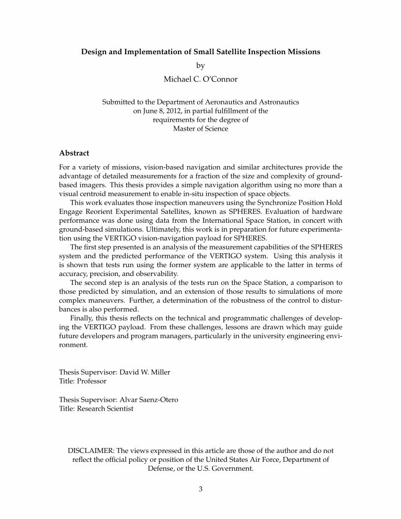
Abstract
For a variety of missions, vision-based navigation and similar architectures provide theadvantage of detailed measurements for a fraction of the size and complexity of ground-based imagers. This thesis provides a simple navigation algorithm using no more than avisual centroid measurement to enable in-situ inspection of space objects.
This work evaluates those inspection maneuvers using the Synchronize Position HoldEngage Reorient Experimental Satellites, known as SPHERES. Evaluation of hardwareperformance was done using data from the International Space Station, in concert withground-based simulations. Ultimately, this work is in preparation for future experimenta-tion using the VERTIGO vision-navigation payload for SPHERES.
The first step presented is an analysis of the measurement capabilities of the SPHERESsystem and the predicted performance of the VERTIGO system. Using this analysis itis shown that tests run using the former system are applicable to the latter in terms ofaccuracy, precision, and observability.
The second step is an analysis of the tests run on the Space Station, a comparison tothose predicted by simulation, and an extension of those results to simulations of morecomplex maneuvers. Further, a determination of the robustness of the control to distur-bances is also performed.
Finally, this thesis reflects on the technical and programmatic challenges of develop-ing the VERTIGO payload. From these challenges, lessons are drawn which may guidefuture developers and program managers, particularly in the university engineering envi-ronment.
Thesis Supervisor: David W. MillerTitle: Professor
Thesis Supervisor: Alvar Saenz-OteroTitle: Research Scientist
DISCLAIMER: The views expressed in this article are those of the author and do notreflect the official policy or position of the United States Air Force, Department of
Defense, or the U.S. Government.
3

4
Acknowledgments
This work was performed primarily under contract FA70001020040 with the US Air Force
Academy, with the support of the Air Force Space and Missile Systems Center as part of
the Space Engineering Academy. The author would also like to thank the Defense Ad-
vanced Research Projects Agency and NASA for their support of the VERTIGO research
and hardware development under contract NNH11CC25C. Finally, the author would like
to recognize the financial support of the National Collegiate Athletic Association via their
Postgraduate Scholarship Program.
5

THIS PAGE INTENTIONALLY LEFT BLANK
6
Contents
1 Introduction 17
1.1 Motivation . . . . . . . . . . . . . . . . . . . . . . . . . . . . . . . . . . . . . . 17
1.1.1 Relevance of Spacecraft Relative Navigation and Inspection . . . . . 17
1.2 Objectives . . . . . . . . . . . . . . . . . . . . . . . . . . . . . . . . . . . . . . 19
1.2.1 Develop Relative Navigation and Inspection Algorithms . . . . . . . 19
1.2.2 Characterize System Performance and Sensor Noise . . . . . . . . . . 20
1.2.3 Quantify Algorithm Performance . . . . . . . . . . . . . . . . . . . . 20
1.3 Previous Work . . . . . . . . . . . . . . . . . . . . . . . . . . . . . . . . . . . . 21
2 Relative Navigation 23
2.1 Vision System Outputs . . . . . . . . . . . . . . . . . . . . . . . . . . . . . . . 23
2.2 Simulation of Vision Measurements . . . . . . . . . . . . . . . . . . . . . . . 24
2.3 Relative Navigation about Unknown Objects . . . . . . . . . . . . . . . . . . 26
2.3.1 Addition of Dead Reckoning . . . . . . . . . . . . . . . . . . . . . . . 27
2.3.2 Addition of Target Rotation Information . . . . . . . . . . . . . . . . 28
3 Inspection 31
3.1 Coverage Quantity . . . . . . . . . . . . . . . . . . . . . . . . . . . . . . . . . 32
3.2 Fuel/Time Tradeoff . . . . . . . . . . . . . . . . . . . . . . . . . . . . . . . . . 33
3.3 Inspection of an Unknown Target . . . . . . . . . . . . . . . . . . . . . . . . . 35
3.3.1 Expected Improvements using Rotation Information . . . . . . . . . 35
3.3.2 Path Optimality . . . . . . . . . . . . . . . . . . . . . . . . . . . . . . . 36
4 Application to the SPHERES System 37
4.1 The SPHERES System . . . . . . . . . . . . . . . . . . . . . . . . . . . . . . . 37
7
4.1.1 What is SPHERES? . . . . . . . . . . . . . . . . . . . . . . . . . . . . . 37
4.1.2 What is VERTIGO? . . . . . . . . . . . . . . . . . . . . . . . . . . . . . 39
4.2 Measurement Fidelity . . . . . . . . . . . . . . . . . . . . . . . . . . . . . . . 42
4.2.1 Vision System Fidelity . . . . . . . . . . . . . . . . . . . . . . . . . . . 43
4.2.2 Metrology System Fidelity . . . . . . . . . . . . . . . . . . . . . . . . . 48
4.3 Tests and Test Design . . . . . . . . . . . . . . . . . . . . . . . . . . . . . . . . 49
4.3.1 Target Translation . . . . . . . . . . . . . . . . . . . . . . . . . . . . . . 50
4.3.2 Vision System Noise . . . . . . . . . . . . . . . . . . . . . . . . . . . . 51
4.3.3 Inspector Motion . . . . . . . . . . . . . . . . . . . . . . . . . . . . . . 51
4.3.4 Use of Rotation Information . . . . . . . . . . . . . . . . . . . . . . . . 52
4.4 Success Metrics . . . . . . . . . . . . . . . . . . . . . . . . . . . . . . . . . . . 53
4.4.1 Coverage . . . . . . . . . . . . . . . . . . . . . . . . . . . . . . . . . . . 53
4.4.2 Fuel Use & Time . . . . . . . . . . . . . . . . . . . . . . . . . . . . . . 55
5 Results 57
5.1 Simulation and Station . . . . . . . . . . . . . . . . . . . . . . . . . . . . . . . 57
5.1.1 Station Results . . . . . . . . . . . . . . . . . . . . . . . . . . . . . . . 58
5.1.2 Simulation Results . . . . . . . . . . . . . . . . . . . . . . . . . . . . . 66
5.1.3 Simulation and Station Comparison . . . . . . . . . . . . . . . . . . . 73
5.1.4 Simulation Only . . . . . . . . . . . . . . . . . . . . . . . . . . . . . . 79
5.2 Maneuver Comparisons and Inspection Performance . . . . . . . . . . . . . 88
5.2.1 Target Behavior . . . . . . . . . . . . . . . . . . . . . . . . . . . . . . . 88
5.2.2 2- and 3-D Motion . . . . . . . . . . . . . . . . . . . . . . . . . . . . . 90
5.2.3 Use of Rotation Information . . . . . . . . . . . . . . . . . . . . . . . . 93
5.3 Conclusion . . . . . . . . . . . . . . . . . . . . . . . . . . . . . . . . . . . . . . 95
6 Project Management of the VERTIGO Payload 97
6.1 Design Principles . . . . . . . . . . . . . . . . . . . . . . . . . . . . . . . . . . 98
6.1.1 Product Design . . . . . . . . . . . . . . . . . . . . . . . . . . . . . . . 98
6.1.2 Process Design . . . . . . . . . . . . . . . . . . . . . . . . . . . . . . . 109
6.2 Timeline and Earned Value Analysis . . . . . . . . . . . . . . . . . . . . . . . 119
6.2.1 Initial Design Period . . . . . . . . . . . . . . . . . . . . . . . . . . . . 120
6.2.2 Design Completion . . . . . . . . . . . . . . . . . . . . . . . . . . . . . 121
8
6.2.3 Initial Build and Test . . . . . . . . . . . . . . . . . . . . . . . . . . . . 123
6.2.4 Flight Hardware . . . . . . . . . . . . . . . . . . . . . . . . . . . . . . 125
6.3 Lessons Learned . . . . . . . . . . . . . . . . . . . . . . . . . . . . . . . . . . . 125
7 Conclusion 129
7.1 Conclusions . . . . . . . . . . . . . . . . . . . . . . . . . . . . . . . . . . . . . 129
7.2 Future Work . . . . . . . . . . . . . . . . . . . . . . . . . . . . . . . . . . . . . 130
A VERTIGO Inspection Maneuver Codes 133
A.1 Simple Maneuvers . . . . . . . . . . . . . . . . . . . . . . . . . . . . . . . . . 133
A.2 Advanced Maneuvers . . . . . . . . . . . . . . . . . . . . . . . . . . . . . . . 141
A.3 Example Code using Video Data . . . . . . . . . . . . . . . . . . . . . . . . . 152
B VERTIGO System Requirements 169
9

THIS PAGE INTENTIONALLY LEFT BLANK
10
List of Figures
2-1 Inertial and relative frames . . . . . . . . . . . . . . . . . . . . . . . . . . . . 25
2-2 Filtering and Centroiding . . . . . . . . . . . . . . . . . . . . . . . . . . . . . 27
3-1 Feature Tracking and Reacquisition by Angle . . . . . . . . . . . . . . . . . . 33
3-2 Shortest Inspection Path on a Sphere . . . . . . . . . . . . . . . . . . . . . . . 36
4-1 A SPHERES satellite . . . . . . . . . . . . . . . . . . . . . . . . . . . . . . . . 38
4-2 SPHERES Global Metrology System . . . . . . . . . . . . . . . . . . . . . . . 38
4-3 VERTIGO “Goggles” Assembly . . . . . . . . . . . . . . . . . . . . . . . . . . 39
4-4 VERTIGO Basic Inspection Path . . . . . . . . . . . . . . . . . . . . . . . . . . 42
4-5 VERTIGO System Block Diagram . . . . . . . . . . . . . . . . . . . . . . . . . 43
4-6 Pinhole camera model, X-Z plane . . . . . . . . . . . . . . . . . . . . . . . . . 44
4-7 Pinhole camera model, X-Y plane . . . . . . . . . . . . . . . . . . . . . . . . . 46
4-8 Stereo Camera Combined Field of View . . . . . . . . . . . . . . . . . . . . . 54
4-9 Target Object Surface Visibility . . . . . . . . . . . . . . . . . . . . . . . . . . 54
5-1 Planar Inspection: Position Data during Stationary Target Test . . . . . . . . 59
5-2 Planar Inspection: Relative Position during Stationary Target Test . . . . . . 59
5-3 Planar Inspection: Relative Velocity during Stationary Target Test . . . . . . 60
5-4 Planar Inspection: Inspector Rate during Stationary Target Test . . . . . . . 61
5-5 Planar Inspection: Difference between Z-Rate and Total Angular Rate dur-
ing Stationary Target Test . . . . . . . . . . . . . . . . . . . . . . . . . . . . . 61
5-6 Planar Inspection: Target Rate during Stationary Target Test . . . . . . . . . 62
5-7 Planar Inspection: Position Data during Moving Target Test . . . . . . . . . 62
5-8 Planar Inspection: Relative Position during Moving Target Test . . . . . . . 63
5-9 Planar Inspection: Relative Velocity during Moving Target Test . . . . . . . 64
11
5-10 Planar Inspection: Inspector Rate during Moving Target Test . . . . . . . . . 64
5-11 Planar Inspection: Difference between Z-Rate and Total Angular Rate dur-
ing Moving Target Test . . . . . . . . . . . . . . . . . . . . . . . . . . . . . . . 65
5-12 Planar Inspection: Target Rate during Stationary Target Test . . . . . . . . . 65
5-13 Planar Inspection: Position Data during Moving Target Simulation . . . . . 67
5-14 Planar Inspection: Relative Position during Moving Target Simulation . . . 67
5-15 Planar Inspection: Relative Velocity during Moving Target Simulation . . . 68
5-16 Planar Inspection: Inspector Rate during Moving Target Simulation . . . . . 68
5-17 Planar Inspection: Difference between Z-Rate and Total Angular Rate dur-
ing Moving Target Simulation . . . . . . . . . . . . . . . . . . . . . . . . . . . 69
5-18 Planar Inspection: Position Data during Moving Target Simulation . . . . . 70
5-19 Planar Inspection: Relative Position during Moving Target Simulation . . . 71
5-20 Planar Inspection: Relative Velocity during Moving Target Simulation . . . 71
5-21 Planar Inspection: Inspector Rate during Moving Target Simulation . . . . . 72
5-22 Planar Inspection: Difference between Z-Rate and Total Angular Rate dur-
ing Moving Target Simulation . . . . . . . . . . . . . . . . . . . . . . . . . . . 73
5-23 Planar Inspection: Position Data during “Additional Motion” Simulation . . 81
5-24 Planar Inspection: Relative Position during “Additional Motion” Simulation 81
5-25 Planar Inspection: Inspector Rate during “Additional Motion” Simulation . 82
5-26 Planar Inspection: Position Data during 3D Inspection Simulation . . . . . . 83
5-27 Planar Inspection: Relative Position during 3D Inspection Simulation . . . . 84
5-28 Planar Inspection: Inspector Rate during 3D Inspection Simulation . . . . . 84
5-29 Planar Inspection: Position Data during Long Duration Simulation . . . . . 85
5-30 Planar Inspection: Relative Position during Long Duration Simulation . . . 85
5-31 Planar Inspection: Inspector Rate during Long Duration Simulation . . . . . 86
5-32 Planar Inspection: Position Data during “Rotation” Simulation . . . . . . . . 87
5-33 Planar Inspection: Relative Position during “Rotation” Simulation . . . . . . 87
5-34 Planar Inspection: Inspector Rate during “Rotation” Simulation . . . . . . . 88
5-35 Coverage: ISS Stationary Test . . . . . . . . . . . . . . . . . . . . . . . . . . . 90
5-36 Coverage: ISS Motion Test . . . . . . . . . . . . . . . . . . . . . . . . . . . . . 91
5-37 Coverage: Simulated Additional Motion Test . . . . . . . . . . . . . . . . . . 91
5-38 Coverage: Simulated 3D Inspection Test . . . . . . . . . . . . . . . . . . . . . 92
12
5-39 Coverage: Simulated Long Duration Test . . . . . . . . . . . . . . . . . . . . 93
5-40 Coverage: Simulated Using Rotation Information Test . . . . . . . . . . . . . 94
5-41 Fuel Use: Rotation Information vs Baselines . . . . . . . . . . . . . . . . . . . 94
6-1 Project and Process for Successful Design . . . . . . . . . . . . . . . . . . . . 98
6-2 Understanding your Design . . . . . . . . . . . . . . . . . . . . . . . . . . . . 101
6-3 Building your Hardware . . . . . . . . . . . . . . . . . . . . . . . . . . . . . . 103
6-4 Testing the Product . . . . . . . . . . . . . . . . . . . . . . . . . . . . . . . . . 106
6-5 Control Measurable Performance through Advocacy . . . . . . . . . . . . . 109
6-6 Improving the Process by Learning from Failure . . . . . . . . . . . . . . . . 111
6-7 Developing Project Margin Estimates . . . . . . . . . . . . . . . . . . . . . . . 116
6-8 Cost/Schedule/Performance Weighting at Contract Start . . . . . . . . . . . 119
6-9 Schedule and Spending Progression . . . . . . . . . . . . . . . . . . . . . . . 123
6-10 Cost/Schedule/Performance Weighting at During Hardware Build . . . . . 124
13

THIS PAGE INTENTIONALLY LEFT BLANK
14
List of Tables
5.1 Mass Properties of Modified Target Satellite . . . . . . . . . . . . . . . . . . . 58
5.2 Estimated Navigation Accuracy . . . . . . . . . . . . . . . . . . . . . . . . . . 95
6.1 VERTIGO PDR Software Schedule . . . . . . . . . . . . . . . . . . . . . . . . 99
6.2 VERTIGO CDR Software Schedule . . . . . . . . . . . . . . . . . . . . . . . . 100
6.3 VERTIGO Revised (Dec. 2011) Software Schedule . . . . . . . . . . . . . . . 100
6.4 Post-CDR Hardware Delivery Schedule . . . . . . . . . . . . . . . . . . . . . 104
6.5 VERTIGO Initial Delivery Schedule . . . . . . . . . . . . . . . . . . . . . . . . 119
6.6 VERTIGO Post-PDR Delivery Schedule . . . . . . . . . . . . . . . . . . . . . 121
6.7 VERTIGO Post-CDR Delivery Schedule . . . . . . . . . . . . . . . . . . . . . 123
6.8 VERTIGO Testing Schedule (Spring 2012) . . . . . . . . . . . . . . . . . . . . 124
6.9 VERTIGO Realized Delivery Schedule . . . . . . . . . . . . . . . . . . . . . . 125
15

THIS PAGE INTENTIONALLY LEFT BLANK
16
Chapter 1
Introduction
1.1 Motivation
Since the launch of the first artificial satellites over 50 years ago, there has always been a na-
tional interest in maintaining the high ground in every sense of the phrase. In resource con-
strained environments, certain advanced concepts provide value disproportionate to their
costs. Vision-based navigation, especially on small servicing satellites hold the promise of
being one such concept that delivers value in a way no other type of small system can.
1.1.1 Relevance of Spacecraft Relative Navigation and Inspection
Spacecraft design, launch, and operation are expensive and often risky undertakings. A
major space-based observatory such as the Hubble Space Telescope, which has a lifetime
cost estimated at $11 billion represents a significant investment of human and financial
capital[1]. Hubble’s successor, the James Webb Space Telescope is expected to cost even
more[2]. In the latter case, as Lagrange point orbit puts it far out of the reach of current
manned spacecraft and therefore would need to be serviced robotically if a problem were
to arise. The signal delays associated with such an orbit, coupled with complex orbital
dynamics about a Lagrange point preclude teleoperated systems. In order to effectively
diagnose failures, a free-flying spacecraft must be able to autonomously inspect the dam-
aged craft.
This ability to observe and repair a damaged spacecraft via a small inspector presents
a risk mitigation strategy for future missions. Commercial ventures may also be more cost
17
effective in the case of servicing and attendant volume savings[3], while in-situ spacecraft
salvage is currently an open research field[4]. In each case, solving the problem requires
the ability to inspect a spacecraft of unknown condition from a distance that is far enough
away to preclude a collision risk, but close enough to provide accurate resolution.
Long duration missions in earth orbit, such as those on the space station, lend them-
selves to human EVA to repair and maintenance. Missions travelling out of Earths mag-
netic field which require repairs would put astronauts at greater risk on two fronts: in-
creased environmental risk to the spacewalker and an inability to return injured astronauts
quickly to Earth. Autonomous inspector vehicles with the ability to identify problems
through computer vision or other sensor systems provide a safer alternative for diagnosis,
with the potential for follow-up repairs by crew.Before that can be realized, the inspection
problem should first be solved in the relative safety of low earth orbit.
Large modern spacecraft are designed with significant redundancies as the forces of
time and the space environment combine to cause part and system failures. Redundancy
provides an element of reliability, but at the cost of increased mass and complexity as entire
systems and subsystems must be duplicated. The ability to repair or replace single failed
parts rather than design backup systems into a satellite has the potential to reduce costs
by reducing the launch mass. Commercial systems on the ground often take this approach
— after all, a car has but one engine. Even if redundancy is built in, the ability to install
replacements, as was done during Hubble servicing missions can extend mission lifetimes
many times the design lifetime for a fraction of the cost of a new system.
In each of the potential applications of in-situ inspection described above, the operat-
ing environments are very different. In each, however, the use of relative measurements
between inspector and target are preferable to more global sensors or any earth-based ob-
servatories. In GEO orbits GPS measurements suffer from position errors on the orders
of meters to tens of meters[5], errors which are compounded by solar fluctuations and
their attendant ionospheric disturbances[6]. For close inspections such errors are unac-
ceptably large, especially when collision avoidance is a high priority. Additional problems
arise when an inspection target is uncooperative and GPS measurements or other global
measurements are therefore unavailable[7]. Star trackers may be problematic in determin-
ing relative position to a target: if they are not overwhelmed by reflected solar light from
the inspection target, their view of the starfield may be obstructed by a complex shape.
18
Ground-based radars are also of limited utility because of the distances and perspective
involved. When the inspector eclipses the ground station, the problem is only further
complicated. As mentioned before, using ground-based sensors also introduces time de-
lays due to light-speed propagation and processing time[8]. In GEO this delay is on the
order of seconds; for missions beyond that point, the delays grow significantly longer in
proportion to the increased distance.
These physical constraints point to the need for space-based inspector vehicles using
relative measurements to maneuver around a target object, and to do so safely (without
colliding) and uncooperatively (no information passed from target to inspector). Further-
more, in contrast to other methods[9], the inspection should be performed with no a priori
knowledge of the target.
1.2 Objectives
To satisfy the mission requirements for a space-based inspector, there are a handful of tasks
which this thesis aims to address.
1.2.1 Develop Relative Navigation and Inspection Algorithms
The first objective is to develop algorithms to perform inspections of an unknown, poten-
tially spinning and tumbling, target object in order to build up a 3D map of the target. This
task is split into two parts:
1. Relative Navigation The ability to move about using measurements of a target object
in the body frame of the inspector. These measurements must not be in reference to
any “global” frame, but instead must be described as movements of the target in the
inspector’s field of view.
2. Inspection The movement of the inspector about the target object for the purpose of
providing a vision payload with a view of the target.
An algorithm which combines these two approaches should enable an inspector to
view all surfaces of a target object, and do so with no reference other than target itself,
as well as onboard inertial navigation sensors like gyroscopes and accelerometers. The
19
combination of Inspection and Relative Navigation elements should allow for planning of
paths around an unknown object.
Additionally, the algorithm should be as simple as possible to reduce the processing
burden and make the algorithm applicable to as many space systems as possible.
Notionally, the algorithm should not require any information about the target object’s
rotation states. By discarding or not collecting this information, the algorithm should allow
for inspections on a larger set of objects, including those that are rotating at high rates.
1.2.2 Characterize System Performance and Sensor Noise
This thesis must also develop a model of the vision system to be used and to compare that
model with the existing SPHERES satellite system, both in simulation and in ISS testing.
Characterizing sensor noise allows for the application of the SPHERES system to the
to-be-launched vision system that this thesis seeks to support. By comparing the noise
sources and noise characteristics of the SPHERES metrology and inertial sensors to those
predicted in a vision system, an understanding of the expected performance of the inte-
grated inspection system can be gained.
1.2.3 Quantify Algorithm Performance
In order to apply the navigation and inspection algorithms that this thesis develops, the
performance of the inspector system must be assessed with a number of characteristics in
mind. The most significant of those performance characteristics are:
1. Fuel Efficiency Minimizing fuel use in an inspection maneuver is preferred. This
will be measured in the amount of CO2 fuel used by the test satellites.
2. Time Efficiency Faster inspections are desired, though more inspection time pro-
vides better coverage. Algorithms which minimize the time to complete an inspec-
tion are preferred.
3. Coverage Each algorithm must provide a full view of an unknown target object to
the inspector satellite. This serves as a constraint on each maneuver. It can also be
used to discriminate between inspection paths based on the quality of inspections —
better inspections provide less oblique views of the target object’s surfaces, and may
provide multiple views of the same surface.
20
These factors will be quantified, and used to compare the performance of different algo-
rithms against one another, as well as the reactions of the given algorithms to target object
behaviors. Additional factors, such as the complexity of the algorithm, code size, and col-
lision risk may also be taken into account, but only to discriminate when the three above
qualities are insufficient.
1.3 Previous Work
Previous work done with vision systems has been used for purposes that vary from space
station assembly (Canadian Space Vision System[10]) to autonomous rendezvous and dock-
ing (DARPAs Orbital Express[11], among others[12]). Relative navigation using vision
sensors may also be the control of autonomous underwater vehicles, with applications
in iceberg-relative navigation[13],[14] and benthic surveys[15],[16]. Research with appli-
cation to vision is ongoing in rendezvous to a tumbling object[17], formation flight[18].
What is well understood is the use of vision and other sensing methods to safely approach
a target prior to a rendezvous maneuver[19]. The success of these methods has been inte-
gral to the US space program, especially in the Shuttle/Station era. Difficulties, however,
arise when the inspection target has an unknown form and no fiducials for easy reference
in navigation. Studies addressing this problem often rely on pre-planned trajectories[20]
around the object or are not easily adaptable to modification of the inspection path based
on the tumbling motion of the target object.
This thesis will outline an algorithm for use in vision-based navigation applications to
perform inspections while maintaining a safe keep-out distance. The algorithm makes use
of range and bearing data which would be available to calibrated stereo cameras, along
with a 3-axis gyroscope onboard the inspecting satellite. The approach will be based on a
rotating inspector that maintains a body-fixed orientation with respect to a target object.
Success will be evaluated primarily on the ability to maintain a safe distance, to maintain
a closed planar path, and demonstrate robustness to certain disturbances. The algorithm
is tested on the SPHERES satellite simulation and onboard the International Space Station
(ISS). The ultrasonic, time-of-flight based navigation system is used on the ISS for truth
measurements.
While more precise algorithms and optimal approaches exist[21], paper focuses on the
21
development of a simple inspection algorithm for use in a wide range of systems in which
the control system may be computationally constrained and to experimentally demon-
strate the effectiveness of that algorithm in a microgravity environment.
The first contribution of this thesis is the development of an algorithm for inspection
that only requires a vision system to compute the range and range rates using a simple
stereo algorithm that can easily be implemented in an embedded system with limited pro-
cessing power. The computational simplicity of this algorithm is due to the fact that it does
not need to compute the relative orientation[22], between frames. Instead, it dead reckons
its position on a spherical surface surrounding the target object using its gyroscopes. The
secondary contribution of this paper is an experimental validation of this algorithm in
a microgravity environment (i.e. the International Space Station) using a gyroscope and
simulated range measurements. This experiment showed that the amount of vertical drift
during a 3 minute test was less than 10 degrees for a stationary target, with 25-minute
simulations showing less than 12 degrees. The third contribution of this paper is an error
analysis to compare the estimation accuracy between the simulated range measurements
and what is expected of an actual stereo vision system.
22
Chapter 2
Relative Navigation
2.1 Vision System Outputs
Stereo cameras, LIDAR/RADAR, structured light systems, and other “vision” systems
provide information about objects in their field of view that include depth, motion, and
a host of surface properties. Each of these systems addresses the same problem using
different hardware, but the principles are the same. Just as LIDAR provides relative dis-
tance measurements to a target’s surface, a two-camera (or more) system will provide 3-
dimensional measurements from a reference point to surface features on the target object
that are in view. This is achieved by triangulating a feature which appears in the field
of view of both cameras using knowledge of the distance between the two cameras and
where the object falls on the focal plane of both imagers. Using trigonometric relation-
ships, each feature can be assigned an estimated distance with respect to some pre-defined
reference point. This reference point is customarily placed in the upper left of the leftmost
camera, and range and bearing to a target are the set of 3-D measurements provided by
the cameras. As they are later implemented in the relative navigation algorithm, this range
and bearing is translated into range and horizontal translation measurements.
A typical stereo vision system provides synchronized images from each camera. Each
camera and lens, however, distorts the true image. Therefore, in order to accurately de-
termine the range and bearing to features, the cameras must first be calibrated. This is
accomplished by providing a set of known features, most commonly a checkerboard pat-
tern, and taking a set of images. Since the image of the checkerboard is distorted by the
lenses and cameras, a recursive batch algorithm can be applied to the image set to provides
23
a least-squares estimate of the distortion parameters. After determining these parameters
and creating matricies to undo the distortion, future images can be quickly adjusted to
remove their effects. This process, the particulars of which will not be described in signifi-
cant detail in this thesis, results in image pairs which are undistorted and rectified and are
able to be used for the aforementioned ranging.
After the calibration, since distortions may be considered removed, the images can be
treated as the output of a pinhole camera.
2.2 Simulation of Vision Measurements
Because of the launch schedule of the vision system hardware (described later, in Chapter
4), we do not yet have the capability to use the VERTIGO Goggles stereo cameras on orbit.
Instead, the SPHERES global metrology system was used to simulate stereo vision mea-
surements. It uses a time-of-flight ultrasonic ranging system system. Using measurements
from a set of five ultrasonic beacons placed around the ISS test volume, the satellites are
able to determine their position. Background telemetry over a wireless link allows each
SPHERE to find the location of others in the test area. Differentiating (via an Extended
Kalman Filter) provides velocity measurements, while the time of flight difference be-
tween faces of the SPHERE provides pointing information. To translate from the global
to relative frame, there are a few steps.
The first step is to convert the global position measurements into the body frame. The
process is illustrated in Figure 2-1, which shows the Inspector, Target, and the Inspector’s
body frame. The vector difference allows us to find the length and direction of rB in the
inertial ISS frame:rB(ISS) = rA(ISS)
= rTGT − rINSP
(2.1)
rB(ISS) = rA(ISS)
= rTGT − rINSP
(2.2)
The origin of the coordinate frame, though not important to the relative state, is located at
a point in the center of the test volume framed by the SPHERES ultrasonic beacons. Using
the quaternion calculated by the ultrasonic metrology system, a rotation matrix from the
24
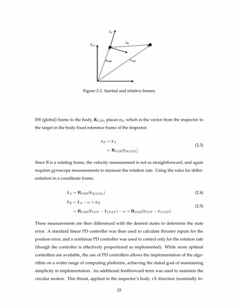
Figure 2-1: Inertial and relative frames
ISS (global) frame to the body, RG2B , places rB , which is the vector from the inspector to
the target in the body-fixed reference frame of the inspector.
rB = rA
= RG2B[rB(ISS)](2.3)
Since B is a rotating frame, the velocity measurement is not as straightforward, and again
requires gyroscope measurements to measure the rotation rate. Using the rules for differ-
entiation in a coordinate frame,
rA = RG2B(rB(ISS)) (2.4)
rB = rA − ω × rB
= RG2B(rTGT − rINSP ) − ω ×RG2B(rTGT − rINSP )(2.5)
These measurements are then differenced with the desired states to determine the state
error. A standard linear PD controller was then used to calculate thruster inputs for the
position error, and a nonlinear PD controller was used to control only for the rotation rate
(though the controller is effectively proportional as implemented). While more optimal
controllers are available, the use of PD controllers allows the implementation of the algo-
rithm on a wider range of computing platforms, achieving the stated goal of maintaining
simplicity in implementation. An additional feedforward term was used to maintain the
circular motion. This thrust, applied in the inspector’s body +X direction (nominally to-
25
ward the target), provided the centripetal force to ensure a circular path:
Fx = mrx,goal ∗ ω2goal (2.6)
Forces and torques were then mixed by the propulsion system, which schedules thruster
opening times for a period of up to 200ms every during each 1-second control period.
Once the VERTIGO Goggles are launched to the station, the output from the cameras
will be processed using the Goggles single-board computer. This computer will process
the images and will output the range, rB , and range-rate, rB , using previously developed
thresholding and centroiding algorithms and eliminating the need for the transformations
described in equations 2.1 through 2.5. Initial prototypes of this technique have demon-
strated the capability to provide such relative measurements.
2.3 Relative Navigation about Unknown Objects
The nature of unknown objects means that they may have certain qualities that preclude
simple tracking of features in order to navigate. Quickly rotating objects in particular pose
difficulty to certain classes of algorithms. Systems which have a low framerate compared
to the rotational rate of the target will have difficulty tracking a given feature from frame
to frame. Take for instance, an image processing algorithm that can account for 10 degrees
of angular motion between frames or less, and a system that operates at 10 frames per
second. Since the maximum rotational speed, ωtarget, is defined by
ωtarget = (FPS)(θlimit) (2.7)
An algorithm dependent on feature tracking for relative navigation will fail if the target
object spins faster than 100◦/s, or about 17 RPM in a single axis. Of course higher framer-
ates or more advanced tracking and estimation tools could be used, but to do so would be
computationally intensive, requiring a larger, more complex system and all of the atten-
dant support systems from thermal control to power storage and distribution. For complex
motion, multifaceted or complicated shapes, unfavorable surface textures, or poor lighting
conditions, processing requirements might push the maximum allowable frame-to-frame
angular displacement far lower.
26
Alternatively, a tracking algorithm which does not require tracking of features from
frame to frame could be used in order to move relative to the rotating target. This is the
approach taken by the VERTIGO team.
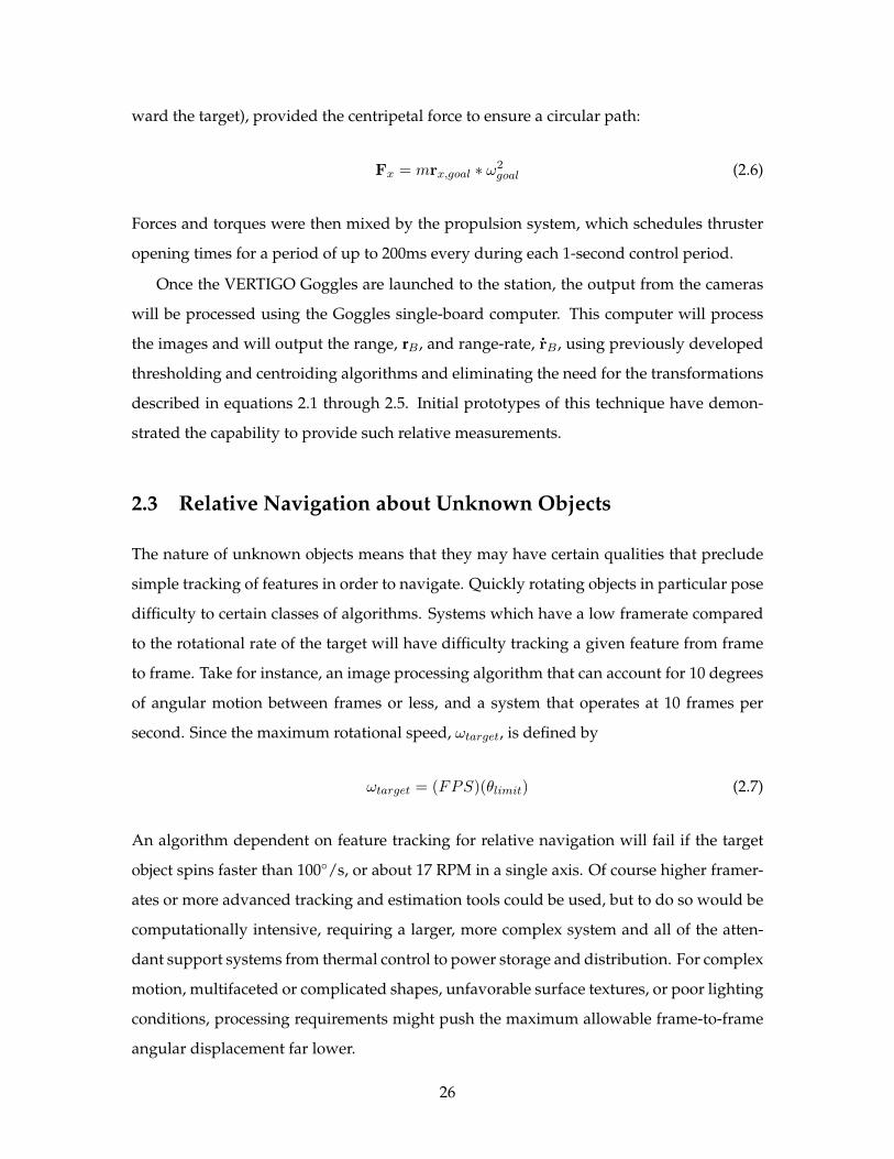
First, operating at about 5 frames per second, the system identifies features in each
image. Next, a filter is applied to the image to exclude those features outside of a set
range (typically beyond 1m from the Inspector, while the size of the baseline excludes
those too close to be observed simultaneously in both cameras). This is done to eliminate
background features associated with testing in an enclosed volume like the International
Space Station, a problem not encountered in an “outdoor” orbital environment where a
starfield at effectively infinite distance is the only background. Next, features are blurred
or blended together and a centroid is calculated. This centroid is then used to estimate
range and translation to the target. The specifics are beyond the scope of this thesis, but
the process unfolds as shown in Figure 2-2.
Figure 2-2: Filtering and Centroiding
2.3.1 Addition of Dead Reckoning
If the only goal of an inspection was to maintain orientation and relative distance, then
processed vision information would be all that is needed. However, in order to perform
maneuvers around a target object, dead reckoning is necessary. Single integration of gyro-
scopes is particularly useful when estimating the motion of the Inspector about the target.
This is because if control is maintained with regards to range and pointing, calculating the
rotation of the Inspector will provide an estimate of the location in an inertial frame whose
origin is co-located with the center of the target object. This inertial location can be used to
27
develop paths which are most likely to provide global coverage of the target object.
The addition of dead reckoning is straightforward: as gyroscopes typically operate at
a high frequency, measurements can be averaged or filtered over short periods. Given
the estimation of the rotational rate of the Inspector, a simple integrator (1s in frequency
domain, Σ in time) may operate on the filtered rates to estimate the angular displacement.
Since the rotational displacement is so closely related to the linear displacement in a well-
controlled system, the motion in inertial space also falls out. A conversion from spherical
to Cartesian coordinates shows this relationship:
θ =T∑t=0
ωz (2.8)
φ =T∑t=0
ωy (2.9)
x = r cosφ sin θ (2.10)
y = r sinφ sin θ (2.11)
z = r cos θ (2.12)
Should the rotation rate about the body X-axis not be kept to zero, additional terms
would need to be included to account for multi-axis coupling.
Inverting the relationships allows for planning of any trajectory in a coordinate frame
that is body-centered and non-rotating with respect to the target object. This method, it
should be noted, is sensitive to gyroscope noise, and will drift accordingly over extended
periods of time. Tracking features on the target object may in some cases be able to aug-
ment gyroscope measurements, and be filtered to provide better accuracy over longer pe-
riods of time. The addition of target object rotations will allow for additional planning, but
that is beyond the problem scope.
2.3.2 Addition of Target Rotation Information
The addition of the rotation of the target has two implications. The first is that by in-
tegrating the rotation of the target object and combining that information with the dead
reckoning estimation from the Inspector’s gyroscopes, maneuvers and navigation can be
designed to take place in the target’s body frame rather than in an arbitrary inertial frame.
28
This is of particular import for optimal design of inspections, as well as ensuring full cov-
erage. Without the knowledge of the rotation of the target relative to the Inspector, there
may be segments of the target which remain uninspected. Indeed, in certain cases where
the inspection motion matches the target’s rotation an inspection may fail to view more
than a single side of the object of interest.
The knowledge of rotation can be two-tiered. A precise, accurate estimation of the
rotation rates of a target are necessary if that information is to be used actively and con-
tinuously for the purposes of path planning. Such an approach is processor-intensive and
decidedly not simple. It will not be dealt with in this thesis.
On the other hand, the use of a general estimation of the rotation of the target object
can be used to improve efficiency of inspections (this will be discussed in a later section),
as well as for insuring better coverage by fixing the inertial frame in a fourth degree of
freedom, rather than just the original three.
29

THIS PAGE INTENTIONALLY LEFT BLANK
30
Chapter 3
Inspection
Inspection is the movement about an object for the purpose of observing its surface and
developing an estimate of its form, function, or other qualities. For the purpose of the
VERTIGO program, the goal of an inspection maneuver is to build a 3-dimensional map
of the target by collecting, storing, and processing information about its surface features.
Four inspection maneuvers were developed for implementation on the SPHERES sys-
tem (and later use on the SPHERES-VERTIGO combined system). Those maneuvers follow
paths described by the following:
1. Stationary This maneuver holds the Inspector satellite stationary in the relative frame,
only maintaining distance and pointing.
2. Planar This inspection is done by imparting a rotation in one axis, causing the In-
spector to move in a plane.
3. X-shaped This maneuver requires integration of the Inspector’s gyros to estimate
movement about the target in an inertial frame. Rotations are imparted into inspector
body axes one at a time, switching after 90◦ and 360◦ of rotation.
4. Hemispheres This maneuver uses gyroscopes onboard the inspector and an estimate
of the target’s rotation. Using the rotation estimate, the inspector aligns with the
rotational axis, then performs inspections in the “northern” rotational hemisphere,
followed by the “southern” hemisphere and equator, switching when the sum of the
estimated rotation of the target and the Inspector indicates 360◦ of the target have
passed in front of the camera.
31
While the first was developed merely for demonstration purposes and would fail to
provide significant coverage unless the target satellite was rotating and tumbling between
multiple axes, the latter three maneuvers are compared based on their performance ac-
cording to coverage, fuel use, and time to completion metrics.
3.1 Coverage Quantity
Coverage is the measure of the surface of a target object that is “visible” to an inspector
satellite. Given a surface mesh, we can therefore assign a binary ’coverage’ state: 1 if the
mesh section is visible, 0 if it is not. In order to determine if a section of the mesh has been
seen by the inspector, we must check the following qualities:
Viewing angle: Test data from initial Phase II (image processing) algorithms shows
difficulty matching features in consecutive frames if the feature lies on a surface
angled more than 30 degrees from perpendicular relative to the camera boresight.
Therefore, to be considered “viewed,” a point should lie on a surface inclined less
than 30 degrees (see Figure 3-1[23]).
Obstruction: Because we are working with the visible spectrum and solid, opaque
objects, we should omit those which are behind another object. Fortunately, the
SPHERES system does not have any self-occluding surfaces or geometries, save very
small sections around the CO2 tank and the regulator knob, which will be ignored
for this thesis. For our purposes, this excludes only surfaces on the opposite side of
the SPHERE from the inspector.
In view: Clearly, to be considered viewed, the surface should be in view of the cam-
era. Given the camera and lenses selected for the VERTIGO project, as well as the
loss of the edges of the images due to distortion, an assumption of a 30 degree field
of view (half cone) is reasonable.
Because the goal of the VERTIGO inspection is to create a 3-D map of a target ob-
ject, obtaining 100% coverage is desired. This requirement therefore determines when
an inspection is completed. For the cost analysis, coverage serves as a constraint on the
optimization. Considering the likelihood of some sensing and approximation error, an
inspection shall be considered complete when 95% of the surface has been inspected.
32
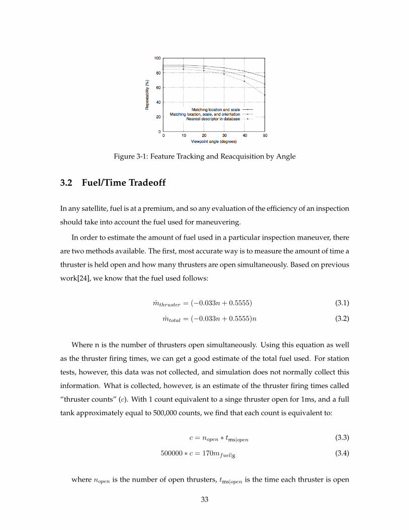
Figure 3-1: Feature Tracking and Reacquisition by Angle
3.2 Fuel/Time Tradeoff
In any satellite, fuel is at a premium, and so any evaluation of the efficiency of an inspection
should take into account the fuel used for maneuvering.
In order to estimate the amount of fuel used in a particular inspection maneuver, there
are two methods available. The first, most accurate way is to measure the amount of time a
thruster is held open and how many thrusters are open simultaneously. Based on previous
work[24], we know that the fuel used follows:
mthruster = (−0.033n+ 0.5555) (3.1)
mtotal = (−0.033n+ 0.5555)n (3.2)
Where n is the number of thrusters open simultaneously. Using this equation as well
as the thruster firing times, we can get a good estimate of the total fuel used. For station
tests, however, this data was not collected, and simulation does not normally collect this
information. What is collected, however, is an estimate of the thruster firing times called
“thruster counts” (c). With 1 count equivalent to a singe thruster open for 1ms, and a full
tank approximately equal to 500,000 counts, we find that each count is equivalent to:
c = nopen ∗ tms|open (3.3)
500000 ∗ c = 170mfuel|g (3.4)
where nopen is the number of open thrusters, tms|open is the time each thruster is open
33
(in units of ms), and c is a count. Fuel mass, mfuel|g, is the mass of fuel (in g) in a full CO2
tank.
For the majority of the inspection, 3 thrusters are expected to fire at any given time, and
we assume they operate for about 30% of their 200ms control period every second. This
yields 2942 counts per gram of fuel. Counts are reported in both simulation and state of
health data returned during SPHERES tests. Therefore, by tracking the thruster counts, we
may estimate the rate of fuel use.
Fuel, however, should not be the only consideration: in two of the most applicable in-
spection scenarios, fuel for a small inspector spacecraft would be a small portion of the
overall mission fuel. In “hosted” spacecraft inspecting a “host” spacecraft like the Inter-
national Space Station or an exploration mission, the host would likely hold large fuel
reserves compared to what is required for relatively simple inspection maneuvers of the
inspector about the host and refueling might be possible. For missions requiring the ren-
dezvous of one spacecraft with another from different orbits, the fuel cost required to attain
and maintain a proper orbit would be significantly larger than maneuvering fuel needs.
With inspections similar to those used for SPHERES, the total ∆V is on the order of cen-
timeters or meters per second, compared to orbital maneuvers which may range in the 10s
to 1000s of m s−1 depending on object size and inspection speed. In each of these cases,
the criticality of failures that demand a close visual inspection may hint at an element of
time-criticality. Indeed, in the case of the Space Shuttle, such maneuvering thrusters (RCS)
were even used for attitude control during launch, implying on-orbit maneuvering fuel
was a minor part of the fuel needs [25].
Therefore, time should also be taken into account alongside fuel use. After all, in most
orbits, over an extended period of time, station keeping requirements would cause fuel
use to grow. Furthermore, if an inspection is non-time critical, the use of orbital dynamics
are more fuel efficient and better suited for most inspections than active inspection and
navigation methods. However, if a spacecraft is damaged enough to require an inspection,
or other mission requirements dictate an inspection to be completed before the completion
of one orbit, the inertial methods presented in this paper are better suited than others.
Certainly in missions requiring long-duration transfers, active control is the only option.
As time grows linearly and is always non-negative, conversion for a cost function is
straightforward. Fuel use is also non-negative and monotonically increasing.
34
Combining the two, we get the cost function,
J(mfuel, t) = Qmfuel +Rnt (3.5)
With the constraint
C(x, t) = 0.95 (3.6)
Where C(x, t) is the ratio of coverage of the target object to its total surface area. The con-
stant n is equal to 0.063g s−1 and is used to compare time and mass under the assumption
that a typical SPHERES will finish a full tank of fuel in 45 minutes of test time.
Given n, weights Q and R are then selected to weigh fuel consumption and time, re-
spectively. If both are equal to 1, then fuel use and time are equally weighted when com-
pared to a typical SPHERES test.
3.3 Inspection of an Unknown Target
3.3.1 Expected Improvements using Rotation Information
Of the three inspection paths tested, only the last takes the rotational state information of
the target into account. By doing so, it is expected that this path will minimize the cost
function compared to the other options. Most of the efficiency is expected to come from
the fact that the Inspector can actively take advantage of the rotation of the target rather
than moving in potentially inefficient paths. For instance, if both satellites are have their
body Z axes aligned, if the target rotates about its +Z axis, if the Inspector rotates about its
−Z axis at half the rate, it will see the be able to observe the entire “equator” of the Target
in a third of the time it would take should they rotate in the same direction.
Additionally, the Inspector will be able to use that knowledge to not only perform faster
and more fuel efficient motions, but it may perform transitions quicker because it allows
the integration of the target’s rotation to estimate coverage rather than only the Inspector’s
gyro information.
As noted earlier, it should be emphasized that the use of rotation information from
the target object is not, nor should it be, required for a successful inspection. Such infor-
mation can only improve an inspection, and shouldn’t be the difference between success
and failure. Without the information of the rotation states, however, full coverage can-
35
not be guaranteed without additional precautions, especially in cases where the rotation
rates of the two satellites match in direction, and particularly those where they match in
magnitude. Such cases can be avoided by varying the inspection speeds in order to elimi-
nate potential resonances between inspector and target. Those approaches and the trades
which inform their selection are, however, beyond the scope of this thesis.
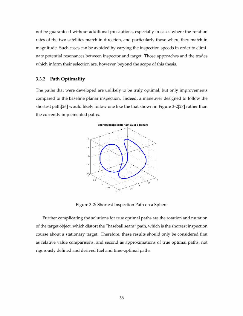
3.3.2 Path Optimality
The paths that were developed are unlikely to be truly optimal, but only improvements
compared to the baseline planar inspection. Indeed, a maneuver designed to follow the
shortest path[26] would likely follow one like the that shown in Figure 3-2[27] rather than
the currently implemented paths.
Figure 3-2: Shortest Inspection Path on a Sphere
Further complicating the solutions for true optimal paths are the rotation and nutation
of the target object, which distort the “baseball seam” path, which is the shortest inspection
course about a stationary target. Therefore, these results should only be considered first
as relative value comparisons, and second as approximations of true optimal paths, not
rigorously defined and derived fuel and time-optimal paths.
36
Chapter 4
Application to the SPHERES System
4.1 The SPHERES System
The Synchronize Position Hold Engage Reorient Experimental Satellites, or SPHERES for
short, are the hardware upon which the navigation and inspection algorithms were de-
veloped and tested. To better understand the constraints of the research, as well as the
realistic nature of the dynamics that are simulated, we first take a look at the current and
future SPHERES program.
4.1.1 What is SPHERES?
The SPHERES satellite testbed was initially developed as part of a capstone design course
in the MIT Space Systems Laboratory (SSL). Since its first launch in 2006 the system has
been hosted aboard the ISS and as of May 2012 has conducted over 30 test sessions in such
varied areas as formation flight, rendezvous and docking, online planning, and STEM
education and outreach. In the 7 years of testing, SPHERES has provided valuable experi-
mental data in a persistent microgravity environment and proven themselves as a valuable
control and navigation testbed.
The system itself consists of ground and space segments, each able to operate in-
dependently of one another. Algorithms are first developed and validated in a high-
fidelity simulation with a MATLAB interface. This simulation, which is constantly be-
ing improved and updated, allows for rapid prototyping of code for control and navi-
gation algorithms. Based on the simulation results, scientists and engineers working on
37
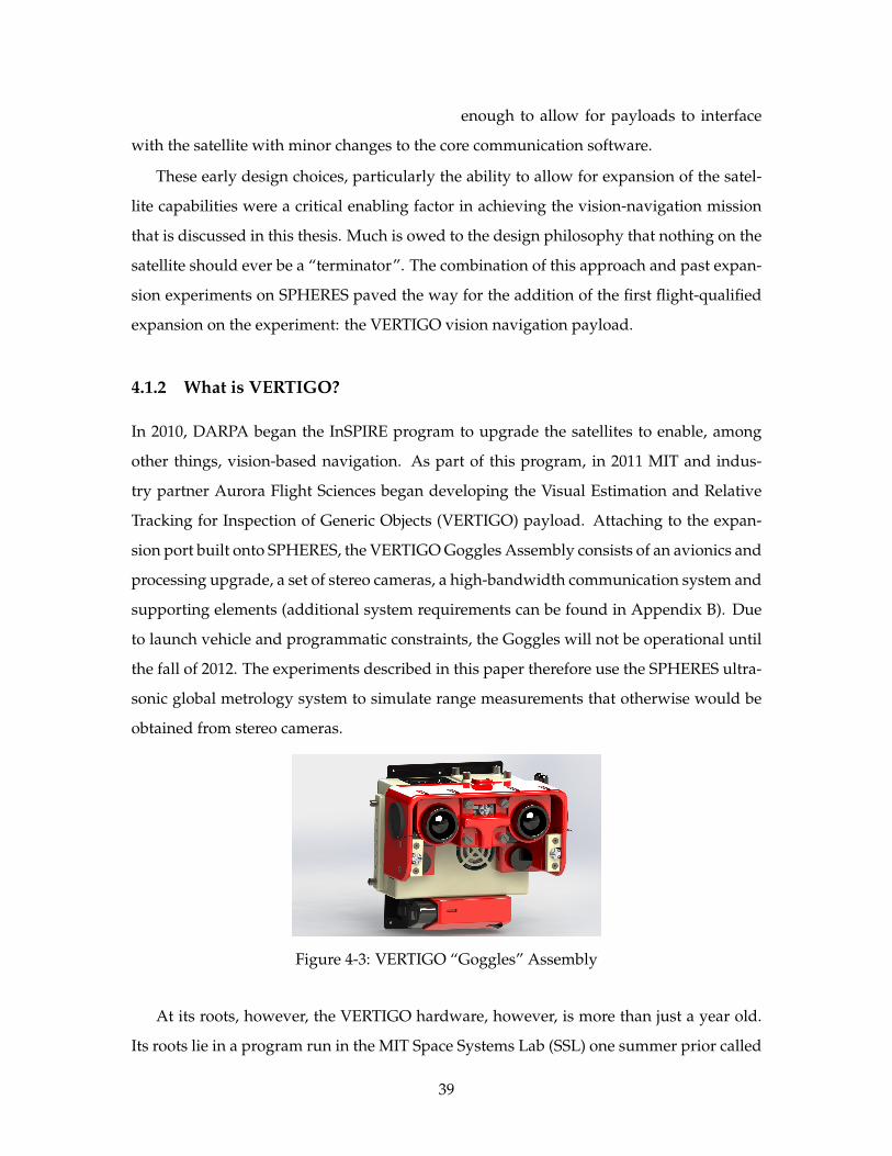
the project verify and validate their code on a flat floor or glass table. After 2-D test-
ing with the SPHERES hardware on ground, the code is packaged and sent for testing
on the ISS. On ground and on station, up to three satellites may typically be used, each
with internal gyroscopes and accelerometers, as well as an external ultrasonic time-of-
flight measurement system[28][29]. The metrology system (Figure 4-2) provides time-
of-flight measurements from five beacons with known locations, to microphones on six
faces of the SPHERES. This data is used for position, velocity, and attitude estimation.
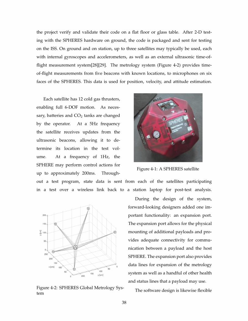
Figure 4-1: A SPHERES satellite
Each satellite has 12 cold gas thrusters,
enabling full 6-DOF motion. As neces-
sary, batteries and CO2 tanks are changed
by the operator. At a 5Hz frequency
the satellite receives updates from the
ultrasonic beacons, allowing it to de-
termine its location in the test vol-
ume. At a frequency of 1Hz, the
SPHERE may perform control actions for
up to approximately 200ms. Through-
out a test program, state data is sent from each of the satellites participating
in a test over a wireless link back to a station laptop for post-test analysis.
Figure 4-2: SPHERES Global Metrology Sys-tem
During the design of the system,
forward-looking designers added one im-
portant functionality: an expansion port.
The expansion port allows for the physical
mounting of additional payloads and pro-
vides adequate connectivity for commu-
nication between a payload and the host
SPHERE. The expansion port also provides
data lines for expansion of the metrology
system as well as a handful of other health
and status lines that a payload may use.
The software design is likewise flexible
38
enough to allow for payloads to interface
with the satellite with minor changes to the core communication software.
These early design choices, particularly the ability to allow for expansion of the satel-
lite capabilities were a critical enabling factor in achieving the vision-navigation mission
that is discussed in this thesis. Much is owed to the design philosophy that nothing on the
satellite should ever be a “terminator”. The combination of this approach and past expan-
sion experiments on SPHERES paved the way for the addition of the first flight-qualified
expansion on the experiment: the VERTIGO vision navigation payload.
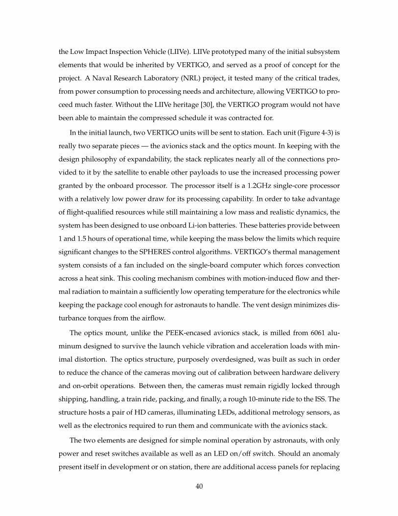
4.1.2 What is VERTIGO?
In 2010, DARPA began the InSPIRE program to upgrade the satellites to enable, among
other things, vision-based navigation. As part of this program, in 2011 MIT and indus-
try partner Aurora Flight Sciences began developing the Visual Estimation and Relative
Tracking for Inspection of Generic Objects (VERTIGO) payload. Attaching to the expan-
sion port built onto SPHERES, the VERTIGO Goggles Assembly consists of an avionics and
processing upgrade, a set of stereo cameras, a high-bandwidth communication system and
supporting elements (additional system requirements can be found in Appendix B). Due
to launch vehicle and programmatic constraints, the Goggles will not be operational until
the fall of 2012. The experiments described in this paper therefore use the SPHERES ultra-
sonic global metrology system to simulate range measurements that otherwise would be
obtained from stereo cameras.
Figure 4-3: VERTIGO “Goggles” Assembly
At its roots, however, the VERTIGO hardware, however, is more than just a year old.
Its roots lie in a program run in the MIT Space Systems Lab (SSL) one summer prior called
39
the Low Impact Inspection Vehicle (LIIVe). LIIVe prototyped many of the initial subsystem
elements that would be inherited by VERTIGO, and served as a proof of concept for the
project. A Naval Research Laboratory (NRL) project, it tested many of the critical trades,
from power consumption to processing needs and architecture, allowing VERTIGO to pro-
ceed much faster. Without the LIIVe heritage [30], the VERTIGO program would not have
been able to maintain the compressed schedule it was contracted for.
In the initial launch, two VERTIGO units will be sent to station. Each unit (Figure 4-3) is
really two separate pieces — the avionics stack and the optics mount. In keeping with the
design philosophy of expandability, the stack replicates nearly all of the connections pro-
vided to it by the satellite to enable other payloads to use the increased processing power
granted by the onboard processor. The processor itself is a 1.2GHz single-core processor
with a relatively low power draw for its processing capability. In order to take advantage
of flight-qualified resources while still maintaining a low mass and realistic dynamics, the
system has been designed to use onboard Li-ion batteries. These batteries provide between
1 and 1.5 hours of operational time, while keeping the mass below the limits which require
significant changes to the SPHERES control algorithms. VERTIGO’s thermal management
system consists of a fan included on the single-board computer which forces convection
across a heat sink. This cooling mechanism combines with motion-induced flow and ther-
mal radiation to maintain a sufficiently low operating temperature for the electronics while
keeping the package cool enough for astronauts to handle. The vent design minimizes dis-
turbance torques from the airflow.
The optics mount, unlike the PEEK-encased avionics stack, is milled from 6061 alu-
minum designed to survive the launch vehicle vibration and acceleration loads with min-
imal distortion. The optics structure, purposely overdesigned, was built as such in order
to reduce the chance of the cameras moving out of calibration between hardware delivery
and on-orbit operations. Between then, the cameras must remain rigidly locked through
shipping, handling, a train ride, packing, and finally, a rough 10-minute ride to the ISS. The
structure hosts a pair of HD cameras, illuminating LEDs, additional metrology sensors, as
well as the electronics required to run them and communicate with the avionics stack.
The two elements are designed for simple nominal operation by astronauts, with only
power and reset switches available as well as an LED on/off switch. Should an anomaly
present itself in development or on station, there are additional access panels for replacing
40
hard drives and a breakout connector which allows for mouse and keyboard inputs. Both
wifi and ethernet connections are available for high speed communication between the
Goggles and the commanding computer, bypassing the considerably slower SPHERES RF
communications. This connection allows for real-time streaming video and download of
large data files between the Goggles and the ISS computers.
That communication is managed, as are all operations, by a GUI running on a laptop
on the ISS. The GUI allows for the astronaut operator to select, load, and operate test
programs and monitor their progress. The VERTIGO plug-in to the SPHERES GUI also
handles the aforementioned video feed to the astronaut crew. This provides additional
feedback beyond what is typically available to ground observers, and provides a more
interesting experience for operators.
Each of these design elements was built to achieve a two-fold mission. The first was to
maintain the flexibility and usability of the SPHERES system as a student-usable, expand-
able testbed. The second, more particular goal, was to support the development of con-
trol, navigation, and other vision-based navigation investigations with space applications.
With VERTIGO, MIT hopes to test out algorithms with application to on-orbit inspection,
failure diagnostics, rendezvous and docking, assembly, and a host of other missions that
vision sensors enable.
The profile for the current VERTIGO mission calls for three phases. The first phase (cre-
atively named Phase I) includes an initial inspection of an unknown object which gathers
information about that object from a “safe” distance with an expectation of near-global
coverage of the target object. The second phase (Phase II) is a pause to allow the Goggles
to process the inspection data to build a 3D map of the target using techniques such as
bundle adjustment[31] or simultaneous localization and mapping(SLAM)[32]. The third
and final phase (Phase III) consists of relative navigation using the 3D map to perform a
closer inspection or to use the object as a stepping-stone or reference point to inspections
further afield. This thesis primarily addresses the first phase.
The phase begins with the target object in view of the cameras of the inspector satellite
(it is assumed that the lost in space problem has been solved on the SPHERES platform
and is beyond the scope of the VERTIGO project). With the target in view, the inspector
may make an estimation of the center of the object using thresholding and centroiding
algorithms[33]. For now, we begin with an assumption that the target object is stationary;
41
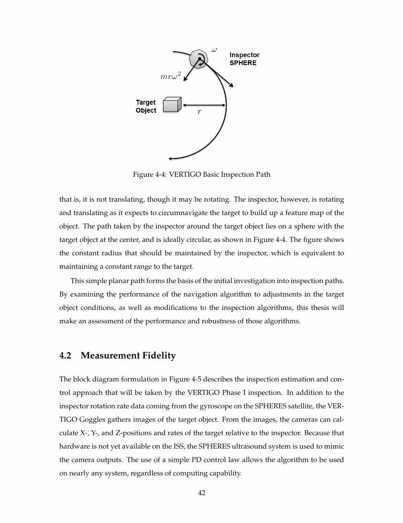
Figure 4-4: VERTIGO Basic Inspection Path
that is, it is not translating, though it may be rotating. The inspector, however, is rotating
and translating as it expects to circumnavigate the target to build up a feature map of the
object. The path taken by the inspector around the target object lies on a sphere with the
target object at the center, and is ideally circular, as shown in Figure 4-4. The figure shows
the constant radius that should be maintained by the inspector, which is equivalent to
maintaining a constant range to the target.
This simple planar path forms the basis of the initial investigation into inspection paths.
By examining the performance of the navigation algorithm to adjustments in the target
object conditions, as well as modifications to the inspection algorithms, this thesis will
make an assessment of the performance and robustness of those algorithms.
4.2 Measurement Fidelity
The block diagram formulation in Figure 4-5 describes the inspection estimation and con-
trol approach that will be taken by the VERTIGO Phase I inspection. In addition to the
inspector rotation rate data coming from the gyroscope on the SPHERES satellite, the VER-
TIGO Goggles gathers images of the target object. From the images, the cameras can cal-
culate X-, Y-, and Z-positions and rates of the target relative to the inspector. Because that
hardware is not yet available on the ISS, the SPHERES ultrasound system is used to mimic
the camera outputs. The use of a simple PD control law allows the algorithm to be used
on nearly any system, regardless of computing capability.
42
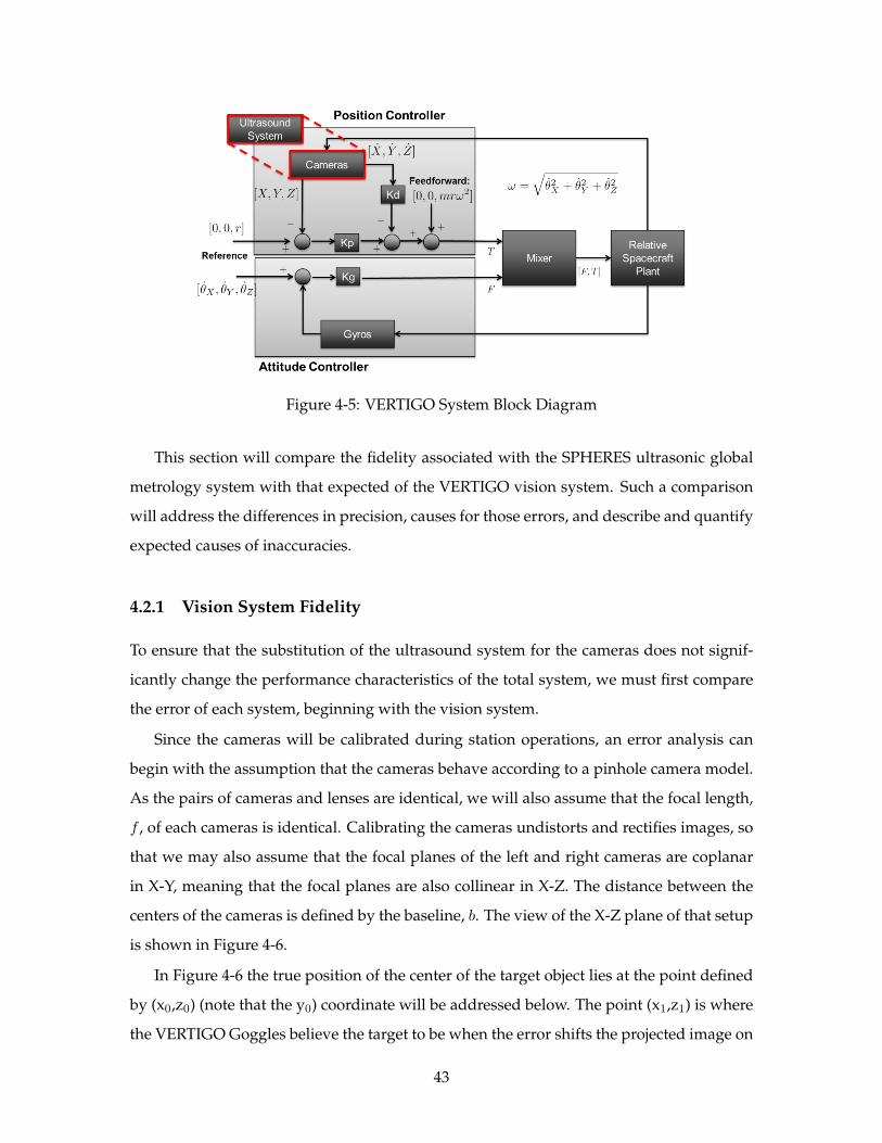
Figure 4-5: VERTIGO System Block Diagram
This section will compare the fidelity associated with the SPHERES ultrasonic global
metrology system with that expected of the VERTIGO vision system. Such a comparison
will address the differences in precision, causes for those errors, and describe and quantify
expected causes of inaccuracies.
4.2.1 Vision System Fidelity
To ensure that the substitution of the ultrasound system for the cameras does not signif-
icantly change the performance characteristics of the total system, we must first compare
the error of each system, beginning with the vision system.
Since the cameras will be calibrated during station operations, an error analysis can
begin with the assumption that the cameras behave according to a pinhole camera model.
As the pairs of cameras and lenses are identical, we will also assume that the focal length,
f , of each cameras is identical. Calibrating the cameras undistorts and rectifies images, so
that we may also assume that the focal planes of the left and right cameras are coplanar
in X-Y, meaning that the focal planes are also collinear in X-Z. The distance between the
centers of the cameras is defined by the baseline, b. The view of the X-Z plane of that setup
is shown in Figure 4-6.
In Figure 4-6 the true position of the center of the target object lies at the point defined
by (x0,z0) (note that the y0) coordinate will be addressed below. The point (x1,z1) is where
the VERTIGO Goggles believe the target to be when the error shifts the projected image on
43
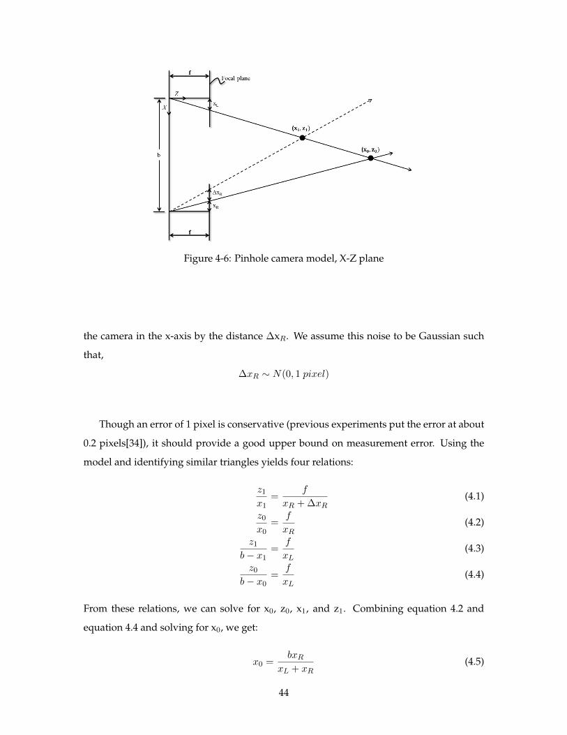
Figure 4-6: Pinhole camera model, X-Z plane
the camera in the x-axis by the distance ∆xR. We assume this noise to be Gaussian such
that,
∆xR ∼ N(0, 1 pixel)
Though an error of 1 pixel is conservative (previous experiments put the error at about
0.2 pixels[34]), it should provide a good upper bound on measurement error. Using the
model and identifying similar triangles yields four relations:
z1x1
=f
xR + ∆xR(4.1)
z0x0
=f
xR(4.2)
z1b− x1
=f
xL(4.3)
z0b− x0
=f
xL(4.4)
From these relations, we can solve for x0, z0, x1, and z1. Combining equation 4.2 and
equation 4.4 and solving for x0, we get:
x0 =bxR
xL + xR(4.5)
44
Placing equation 4.5 back into equation 4.2, we find that
z0 =bf
xL + xR(4.6)
Returning to equations equations 4.1 and 4.3, we can solve each for z1, set them equal, and
algebraically find x1. A second substitution solves for z1:
z1 =x1f
xR + ∆xR=f(b− x1)
xL
x1 =b(xR + ∆xR)
xL + xR + ∆xR(4.7)
z1 =bf
xL + xR + ∆xR(4.8)
Using the typical inspection VERTIGO inspection position yields an (x0,z0) of (70cm,
4.5cm). With a pixel size of 6µm, the 1-pixel error yields (x1,z1) of (68.9cm, 4.57cm), for an
absolute position error of 0.7mm in x and 1.1cm in the z-axis.
The general form of the error is:
∆x = x1 − x0
=b(xR + ∆xR)
xL + xR + ∆xR− bxRxL + xR
=b(xR + ∆xR)(xL + xR) − bxr(xL + xR + ∆xR)
(xL + xR + ∆xR)(xL + xR)
∆x =b(xL∆xR)
(xL + xR + ∆xR)(xL + xR)(4.9)
∆z = z1 − z0
=x1f
xR + ∆xR=f(b− x1)
xL− bf
xL + xR
∆z =−fb(∆xR)
(xL + xR + ∆xR)(xL + xR)(4.10)
This, however, is only half of the story, as the X-Y plane also provides error sources.
A similar approach can be used to approximate the position estimation error that results
45
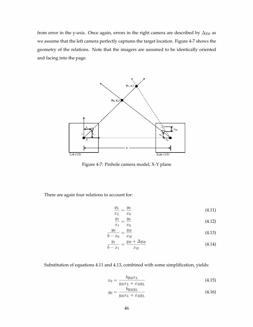
from error in the y-axis. Once again, errors in the right camera are described by ∆yR as
we assume that the left camera perfectly captures the target location. Figure 4-7 shows the
geometry of the relations. Note that the imagers are assumed to be identically oriented
and facing into the page.
Figure 4-7: Pinhole camera model, X-Y plane
There are again four relations to account for:
yLxL
=y0x0
(4.11)
y1x1
=y0x0
(4.12)
y0b− x0
=yRxR
(4.13)
y1b− x1
=yR + ∆yR
xR(4.14)
Substitution of equations 4.11 and 4.13, combined with some simplification, yields:
x0 =byRxL
yRxL + xRyL(4.15)
y0 =byRyL
yRxL + xRyL(4.16)
46
while the combination of Equations 4.12 and 4.14 will give:
x1 = bxL(yR + ∆yR)
xLyR + yLxR + ∆yRxL(4.17)
y1 = byL(yR + ∆yR)
xLyR + yLxR + ∆yRxL(4.18)
Therefore, the combination of the two will yield an error that follows
∆x = x1 − x0
= bxL(yR + ∆yR)
xLyR + yLxR + ∆yRxL− byRxLyRxL + xRyL
∆x =bxLxRyL(∆yR)
(xLyR + yLxR + ∆yRxL)(yRxL + xRyL)(4.19)
∆y = y1 − y0
= byL(yR + ∆yR)
xLyR + yLxR + ∆yRxL− byRyLyRxL + xRyL
∆y =bxRy
2L(∆yR)
(xLyR + yLxR + ∆yRxL)(yRxL + xRyL)(4.20)
During an inspection, the target object is expected to be kept in the camera frame at
approximately:
x0
y0
z0
=
4.5cm
−2.25cm
70cm
Additionally, the parameters of the cameras selected for VERTIGO include a focal
length (f ) of 2.8 mm, a baseline (b) of 9cm, and square pixels that are 6µm on a side.
By starting with these values, substitution allows us to find that as a result of pixel
error in the X-axis,
47
∆x = 0.74mm
∆z = 1.15cm
while pixel error in the Y-axis gives
∆x = 0.78mm
∆y = 1.6mm
This leaves us with two values for the standard deviation of the x error. Because the
probability of errors in the x- and y-directions can be treated as independent random vari-
ables, the total variance of x is the sum of the variances due to each pixel error:
σ2x−total = σ2x|xError + σ2x|yError (4.21)
This works out to 1.7mm. This total error, as will be shown in the next section, is far
below the error that will be introduced by the metrology system. Because of this, it is clear
that any testing which uses the SPHERES metrology system does not provide accuracy
that is unrealistic compared to vision measurements. Further research does need to be
done to confirm this, especially when feature identification is put into the equation, but
these preliminary results show that SPHERES is a valid way to test the vision navigation
algorithms, and do so in a way that demonstrates a worst-case scenario for the sensors.
4.2.2 Metrology System Fidelity
The SPHERES global metrology system, which is made up of a set of 5 ultrasonic beacons,
is triggered when an infrared pulse is emitted within the test volume. After a 10ms delay,
this pulse causes each of the 5 beacons to respond at 20ms intervals, in sequence. Because
the infrared pulse is propagated nearly instantaneously, the beacon locations are known,
and the ultrasonic waves propagate at a known rate, a time-of-flight calculation can de-
termine the range of each satellite ultrasonic sensor and each beacon. Onboard processing
allows the beacons to determine position, velocity, and attitude of each satellite.
48
Errors can arise when additional light sources provide infrared pulses, though such
errors are more likely to cause the processor to reset than to cause one-off errors in estima-
tion. More common errors include variation in the positioning of the beacons themselves,
as well as random noise in the sensors themselves, which may manifest itself as noise on
the calculated satellite position and attitude.
Experience with the system shows that the uncertainty associated with the system has
a precision no worse than 1cm and is accurate to within about 2cm. For position measure-
ments, which require a difference, the variance is therefore summed, which means that
the 1-sigma deviation of the metrology is expected to be accurate only to within 2.8cm in
all directions, even before accounting for quaternion error associated with the metrology.
This is significantly worse than the vision system is expected to perform.
4.3 Tests and Test Design
In order to evaluate the algorithms’ effectiveness in a variety of settings, tests were devel-
oped which stressed the system. A subset of these tests was run in the 6 degree of freedom
microgravity environment onboard the ISS, while the full set was evaluated in a simulation
developed by previous SPHERES researchers.
By using the results from the ISS data and comparing it to the simulation output, it is
possible to develop an understanding of how well the simulation approximates the real
world system. Further, by identifying the differences, it is possible to determine the mode
of the divergence.
The tests will evaluate the impact of the following variables on the behavior of the
inspection system:
1. Target Behavior Movement of the target object toward, away from, and perpendic-
ular to the field of view will demonstrate the robustness of the algorithm to uncer-
tainty in the object’s shape. More directly, it will also show the robustness of the
inspection and relative navigation algorithms as implemented with SPHERES con-
trollers to motion of the target.
2. Vision System Noise Vision system noise may impact the accuracy of the controller.
The noise on the metrology measurements should provide an upper bound on the
49
vision system noise, but variation can be explored through by adding additional
noise into the simulation.
3. Motion Dimension Initial movement is 2-dimensional. Tests should demonstrate
the impact of introducing a 3rd dimension. An exploration of non-planar motion
may also impact the optimality of the maneuver.
4. Rotation Information Taking the rotation of the target object into account may change
the most efficient path.
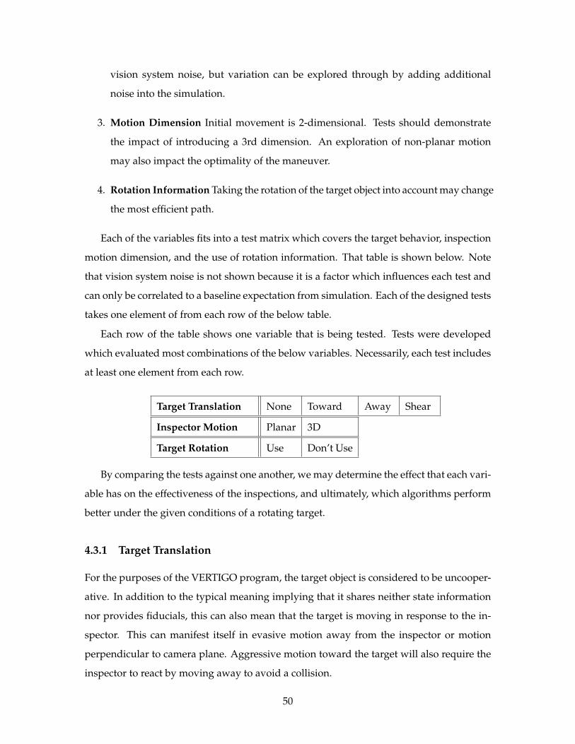
Each of the variables fits into a test matrix which covers the target behavior, inspection
motion dimension, and the use of rotation information. That table is shown below. Note
that vision system noise is not shown because it is a factor which influences each test and
can only be correlated to a baseline expectation from simulation. Each of the designed tests
takes one element of from each row of the below table.
Each row of the table shows one variable that is being tested. Tests were developed
which evaluated most combinations of the below variables. Necessarily, each test includes
at least one element from each row.
Target Translation None Toward Away Shear
Inspector Motion Planar 3D
Target Rotation Use Don’t Use
By comparing the tests against one another, we may determine the effect that each vari-
able has on the effectiveness of the inspections, and ultimately, which algorithms perform
better under the given conditions of a rotating target.
4.3.1 Target Translation
For the purposes of the VERTIGO program, the target object is considered to be uncooper-
ative. In addition to the typical meaning implying that it shares neither state information
nor provides fiducials, this can also mean that the target is moving in response to the in-
spector. This can manifest itself in evasive motion away from the inspector or motion
perpendicular to camera plane. Aggressive motion toward the target will also require the
inspector to react by moving away to avoid a collision.
50
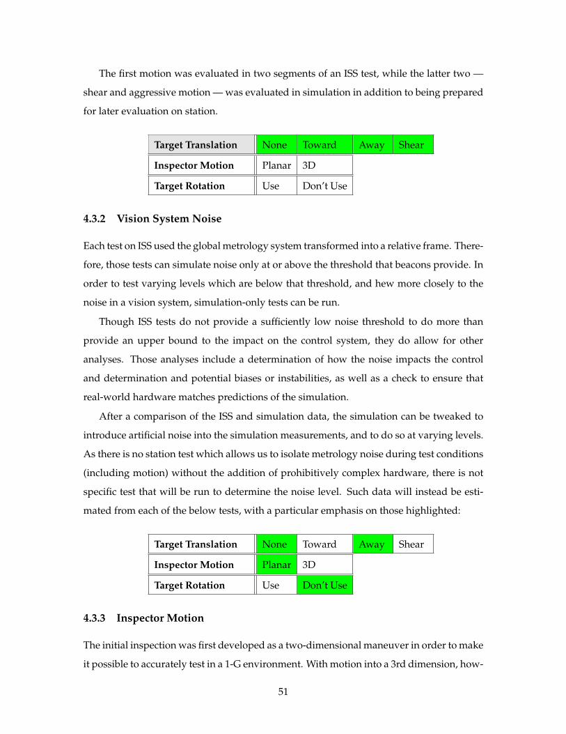
The first motion was evaluated in two segments of an ISS test, while the latter two —
shear and aggressive motion — was evaluated in simulation in addition to being prepared
for later evaluation on station.
Target Translation None Toward Away Shear
Inspector Motion Planar 3D
Target Rotation Use Don’t Use
4.3.2 Vision System Noise
Each test on ISS used the global metrology system transformed into a relative frame. There-
fore, those tests can simulate noise only at or above the threshold that beacons provide. In
order to test varying levels which are below that threshold, and hew more closely to the
noise in a vision system, simulation-only tests can be run.
Though ISS tests do not provide a sufficiently low noise threshold to do more than
provide an upper bound to the impact on the control system, they do allow for other
analyses. Those analyses include a determination of how the noise impacts the control
and determination and potential biases or instabilities, as well as a check to ensure that
real-world hardware matches predictions of the simulation.
After a comparison of the ISS and simulation data, the simulation can be tweaked to
introduce artificial noise into the simulation measurements, and to do so at varying levels.
As there is no station test which allows us to isolate metrology noise during test conditions
(including motion) without the addition of prohibitively complex hardware, there is not
specific test that will be run to determine the noise level. Such data will instead be esti-
mated from each of the below tests, with a particular emphasis on those highlighted:
Target Translation None Toward Away Shear
Inspector Motion Planar 3D
Target Rotation Use Don’t Use
4.3.3 Inspector Motion
The initial inspection was first developed as a two-dimensional maneuver in order to make
it possible to accurately test in a 1-G environment. With motion into a 3rd dimension, how-
51
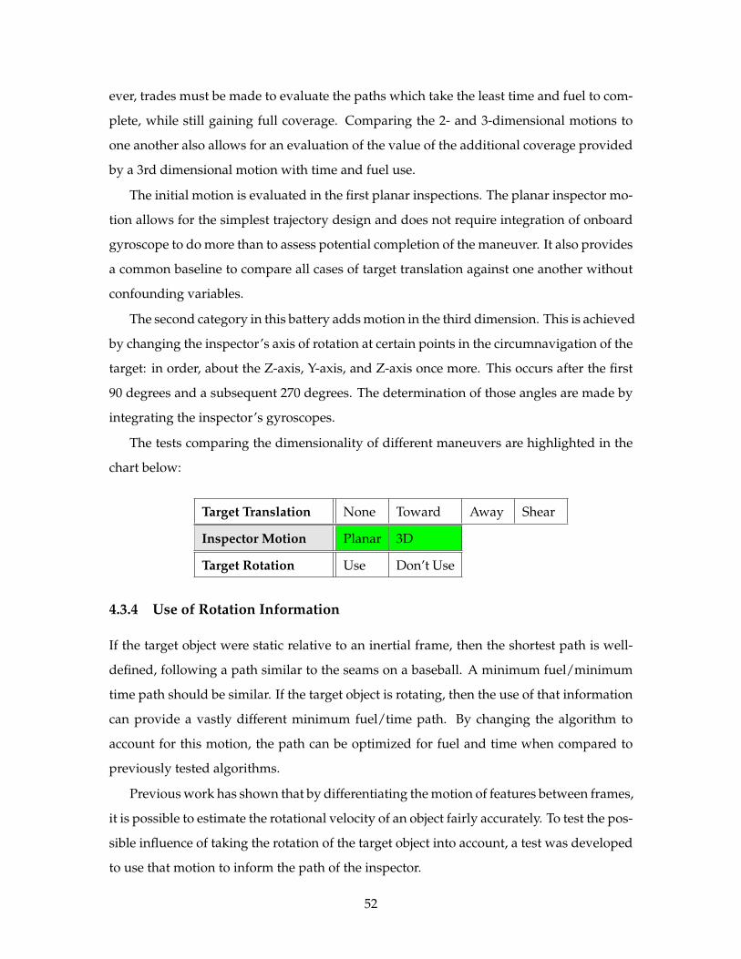
ever, trades must be made to evaluate the paths which take the least time and fuel to com-
plete, while still gaining full coverage. Comparing the 2- and 3-dimensional motions to
one another also allows for an evaluation of the value of the additional coverage provided
by a 3rd dimensional motion with time and fuel use.
The initial motion is evaluated in the first planar inspections. The planar inspector mo-
tion allows for the simplest trajectory design and does not require integration of onboard
gyroscope to do more than to assess potential completion of the maneuver. It also provides
a common baseline to compare all cases of target translation against one another without
confounding variables.
The second category in this battery adds motion in the third dimension. This is achieved
by changing the inspector’s axis of rotation at certain points in the circumnavigation of the
target: in order, about the Z-axis, Y-axis, and Z-axis once more. This occurs after the first
90 degrees and a subsequent 270 degrees. The determination of those angles are made by
integrating the inspector’s gyroscopes.
The tests comparing the dimensionality of different maneuvers are highlighted in the
chart below:
Target Translation None Toward Away Shear
Inspector Motion Planar 3D
Target Rotation Use Don’t Use
4.3.4 Use of Rotation Information
If the target object were static relative to an inertial frame, then the shortest path is well-
defined, following a path similar to the seams on a baseball. A minimum fuel/minimum
time path should be similar. If the target object is rotating, then the use of that information
can provide a vastly different minimum fuel/time path. By changing the algorithm to
account for this motion, the path can be optimized for fuel and time when compared to
previously tested algorithms.
Previous work has shown that by differentiating the motion of features between frames,
it is possible to estimate the rotational velocity of an object fairly accurately. To test the pos-
sible influence of taking the rotation of the target object into account, a test was developed
to use that motion to inform the path of the inspector.
52
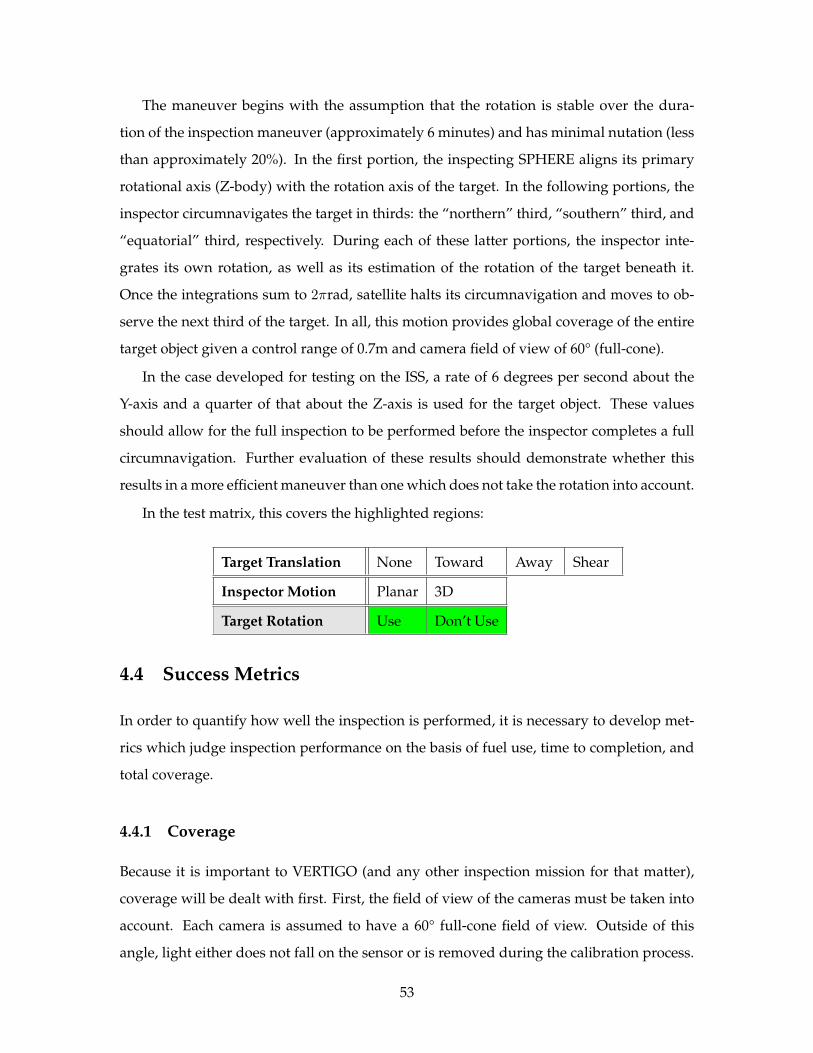
The maneuver begins with the assumption that the rotation is stable over the dura-
tion of the inspection maneuver (approximately 6 minutes) and has minimal nutation (less
than approximately 20%). In the first portion, the inspecting SPHERE aligns its primary
rotational axis (Z-body) with the rotation axis of the target. In the following portions, the
inspector circumnavigates the target in thirds: the “northern” third, “southern” third, and
“equatorial” third, respectively. During each of these latter portions, the inspector inte-
grates its own rotation, as well as its estimation of the rotation of the target beneath it.
Once the integrations sum to 2πrad, satellite halts its circumnavigation and moves to ob-
serve the next third of the target. In all, this motion provides global coverage of the entire
target object given a control range of 0.7m and camera field of view of 60° (full-cone).
In the case developed for testing on the ISS, a rate of 6 degrees per second about the
Y-axis and a quarter of that about the Z-axis is used for the target object. These values
should allow for the full inspection to be performed before the inspector completes a full
circumnavigation. Further evaluation of these results should demonstrate whether this
results in a more efficient maneuver than one which does not take the rotation into account.
In the test matrix, this covers the highlighted regions:
Target Translation None Toward Away Shear
Inspector Motion Planar 3D
Target Rotation Use Don’t Use
4.4 Success Metrics
In order to quantify how well the inspection is performed, it is necessary to develop met-
rics which judge inspection performance on the basis of fuel use, time to completion, and
total coverage.
4.4.1 Coverage
Because it is important to VERTIGO (and any other inspection mission for that matter),
coverage will be dealt with first. First, the field of view of the cameras must be taken into
account. Each camera is assumed to have a 60° full-cone field of view. Outside of this
angle, light either does not fall on the sensor or is removed during the calibration process.
53
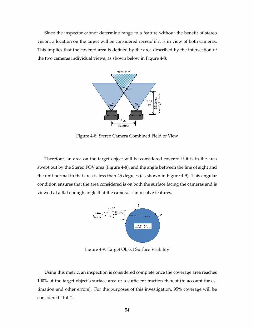
Since the inspector cannot determine range to a feature without the benefit of stereo
vision, a location on the target will be considered covered if it is in view of both cameras.
This implies that the covered area is defined by the area described by the intersection of
the two cameras individual views, as shown below in Figure 4-8:
Figure 4-8: Stereo Camera Combined Field of View
Therefore, an area on the target object will be considered covered if it is in the area
swept out by the Stereo FOV area (Figure 4-8), and the angle between the line of sight and
the unit normal to that area is less than 45 degrees (as shown in Figure 4-9). This angular
condition ensures that the area considered is on both the surface facing the cameras and is
viewed at a flat enough angle that the cameras can resolve features.
Figure 4-9: Target Object Surface Visibility
Using this metric, an inspection is considered complete once the coverage area reaches
100% of the target object’s surface area or a sufficient fraction thereof (to account for es-
timation and other errors). For the purposes of this investigation, 95% coverage will be
considered “full”.
54
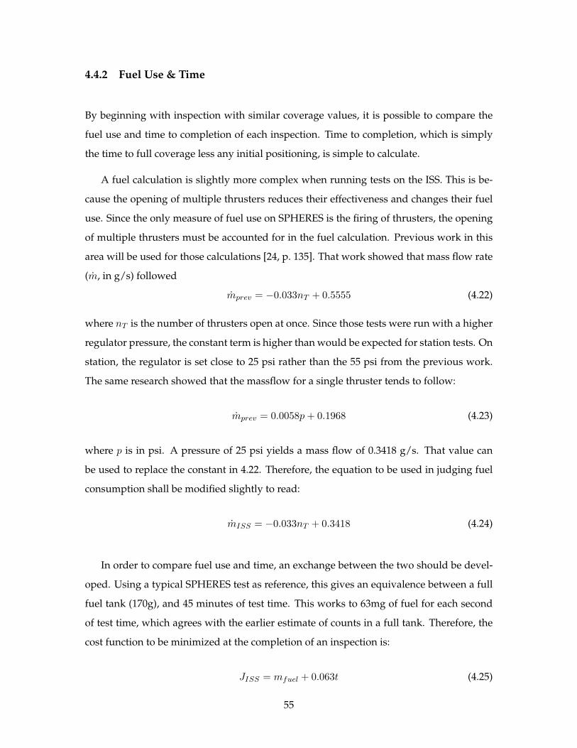
4.4.2 Fuel Use & Time
By beginning with inspection with similar coverage values, it is possible to compare the
fuel use and time to completion of each inspection. Time to completion, which is simply
the time to full coverage less any initial positioning, is simple to calculate.
A fuel calculation is slightly more complex when running tests on the ISS. This is be-
cause the opening of multiple thrusters reduces their effectiveness and changes their fuel
use. Since the only measure of fuel use on SPHERES is the firing of thrusters, the opening
of multiple thrusters must be accounted for in the fuel calculation. Previous work in this
area will be used for those calculations [24, p. 135]. That work showed that mass flow rate
(m, in g/s) followed
mprev = −0.033nT + 0.5555 (4.22)
where nT is the number of thrusters open at once. Since those tests were run with a higher
regulator pressure, the constant term is higher than would be expected for station tests. On
station, the regulator is set close to 25 psi rather than the 55 psi from the previous work.
The same research showed that the massflow for a single thruster tends to follow:
mprev = 0.0058p+ 0.1968 (4.23)
where p is in psi. A pressure of 25 psi yields a mass flow of 0.3418 g/s. That value can
be used to replace the constant in 4.22. Therefore, the equation to be used in judging fuel
consumption shall be modified slightly to read:
mISS = −0.033nT + 0.3418 (4.24)
In order to compare fuel use and time, an exchange between the two should be devel-
oped. Using a typical SPHERES test as reference, this gives an equivalence between a full
fuel tank (170g), and 45 minutes of test time. This works to 63mg of fuel for each second
of test time, which agrees with the earlier estimate of counts in a full tank. Therefore, the
cost function to be minimized at the completion of an inspection is:
JISS = mfuel + 0.063t (4.25)
55

By comparing the ability of different algorithms against one another in terms of fuel
use, we are able to characterize the relative effectiveness of each approach in providing
near-global coverage in the uncertain inspection environment.
56
Chapter 5
Results
This chapter will discuss the data from both station-run tests and simulations. After a
discussion of the performance characteristics of the inspector in both types of tests, a com-
parison will be drawn between the two. Overall, the chapter will examine whether the
simulation is a sufficiently faithful model of the actual system, and what differences must
be accounted for in simulation results.
Following the comparison, the chapter will analyze tests that were run only in simula-
tion. Using the lessons from the comparison between station and simulation data, conclu-
sions will be drawn about the expected performance of the simulation-only tests should
they be run on station.
Finally, there are two additional elements which will be addressed. The first is an
analysis of the gyroscope noise characteristics based on the small 2-test sample of station
data. And finally, a brief analysis of the efficiency of various inspection methods will be
conducted. This latter analysis will conclude which inspection path is the most fuel- and
time-efficient method for inspecting a tumbling target.
5.1 Simulation and Station
This section will describe the results of the tests outlined in Chapter 4, with an emphasis
on Section 4.3. To begin, the results from both station and simulation will be laid out,
and then compared against one another. By comparing the two test methods, it should be
possible to identify the differences and similarities between the two, and in particular the
reasons why they agree or disagree.
57
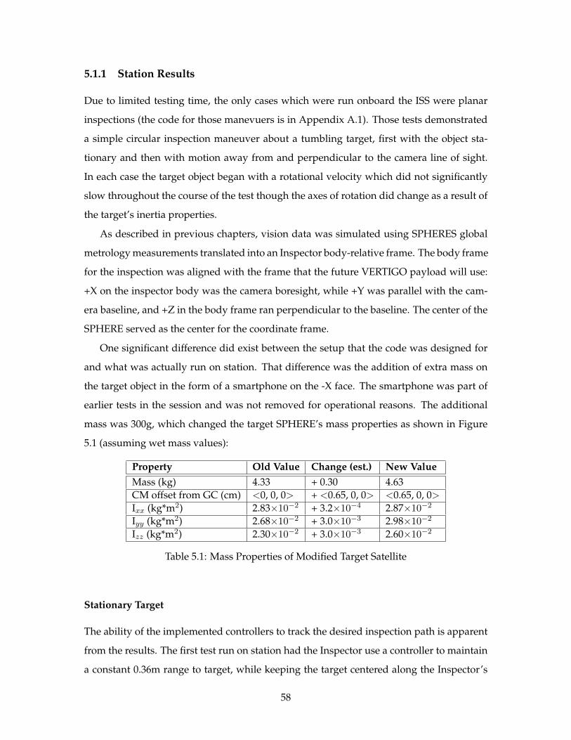
5.1.1 Station Results
Due to limited testing time, the only cases which were run onboard the ISS were planar
inspections (the code for those manevuers is in Appendix A.1). Those tests demonstrated
a simple circular inspection maneuver about a tumbling target, first with the object sta-
tionary and then with motion away from and perpendicular to the camera line of sight.
In each case the target object began with a rotational velocity which did not significantly
slow throughout the course of the test though the axes of rotation did change as a result of
the target’s inertia properties.
As described in previous chapters, vision data was simulated using SPHERES global
metrology measurements translated into an Inspector body-relative frame. The body frame
for the inspection was aligned with the frame that the future VERTIGO payload will use:
+X on the inspector body was the camera boresight, while +Y was parallel with the cam-
era baseline, and +Z in the body frame ran perpendicular to the baseline. The center of the
SPHERE served as the center for the coordinate frame.
One significant difference did exist between the setup that the code was designed for
and what was actually run on station. That difference was the addition of extra mass on
the target object in the form of a smartphone on the -X face. The smartphone was part of
earlier tests in the session and was not removed for operational reasons. The additional
mass was 300g, which changed the target SPHERE’s mass properties as shown in Figure
5.1 (assuming wet mass values):
Property Old Value Change (est.) New ValueMass (kg) 4.33 + 0.30 4.63CM offset from GC (cm) <0, 0, 0> + <0.65, 0, 0> <0.65, 0, 0>Ixx (kg*m2) 2.83×10⁻² + 3.2×10⁻⁴ 2.87×10⁻²
Iyy (kg*m2) 2.68×10⁻² + 3.0×10⁻³ 2.98×10⁻²
Izz (kg*m2) 2.30×10⁻² + 3.0×10⁻³ 2.60×10⁻²
Table 5.1: Mass Properties of Modified Target Satellite
Stationary Target
The ability of the implemented controllers to track the desired inspection path is apparent
from the results. The first test run on station had the Inspector use a controller to maintain
a constant 0.36m range to target, while keeping the target centered along the Inspector’s
58
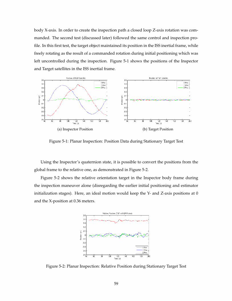
body X-axis. In order to create the inspection path a closed loop Z-axis rotation was com-
manded. The second test (discussed later) followed the same control and inspection pro-
file. In this first test, the target object maintained its position in the ISS inertial frame, while
freely rotating as the result of a commanded rotation during initial positioning which was
left uncontrolled during the inspection. Figure 5-1 shows the positions of the Inspector
and Target satellites in the ISS inertial frame.
(a) Inspector Position (b) Target Position
Figure 5-1: Planar Inspection: Position Data during Stationary Target Test
Using the Inspector’s quaternion state, it is possible to convert the positions from the
global frame to the relative one, as demonstrated in Figure 5-2.
Figure 5-2 shows the relative orientation target in the Inspector body frame during
the inspection maneuver alone (disregarding the earlier initial positioning and estimator
initialization stages). Here, an ideal motion would keep the Y- and Z-axis positions at 0
and the X-position at 0.36 meters.
Figure 5-2: Planar Inspection: Relative Position during Stationary Target Test
59
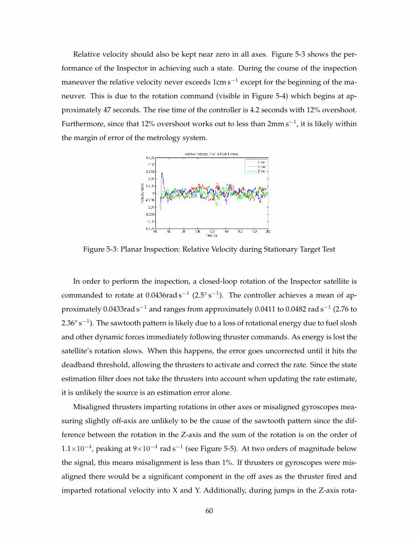
Relative velocity should also be kept near zero in all axes. Figure 5-3 shows the per-
formance of the Inspector in achieving such a state. During the course of the inspection
maneuver the relative velocity never exceeds 1cm s−1 except for the beginning of the ma-
neuver. This is due to the rotation command (visible in Figure 5-4) which begins at ap-
proximately 47 seconds. The rise time of the controller is 4.2 seconds with 12% overshoot.
Furthermore, since that 12% overshoot works out to less than 2mm s−1, it is likely within
the margin of error of the metrology system.
Figure 5-3: Planar Inspection: Relative Velocity during Stationary Target Test
In order to perform the inspection, a closed-loop rotation of the Inspector satellite is
commanded to rotate at 0.0436rad s−1 (2.5° s−1). The controller achieves a mean of ap-
proximately 0.0433rad s−1 and ranges from approximately 0.0411 to 0.0482 rad s−1 (2.76 to
2.36° s−1). The sawtooth pattern is likely due to a loss of rotational energy due to fuel slosh
and other dynamic forces immediately following thruster commands. As energy is lost the
satellite’s rotation slows. When this happens, the error goes uncorrected until it hits the
deadband threshold, allowing the thrusters to activate and correct the rate. Since the state
estimation filter does not take the thrusters into account when updating the rate estimate,
it is unlikely the source is an estimation error alone.
Misaligned thrusters imparting rotations in other axes or misaligned gyroscopes mea-
suring slightly off-axis are unlikely to be the cause of the sawtooth pattern since the dif-
ference between the rotation in the Z-axis and the sum of the rotation is on the order of
1.1×10⁻⁴, peaking at 9×10⁻⁴ rad s−1 (see Figure 5-5). At two orders of magnitude below
the signal, this means misalignment is less than 1%. If thrusters or gyroscopes were mis-
aligned there would be a significant component in the off axes as the thruster fired and
imparted rotational velocity into X and Y. Additionally, during jumps in the Z-axis rota-
60
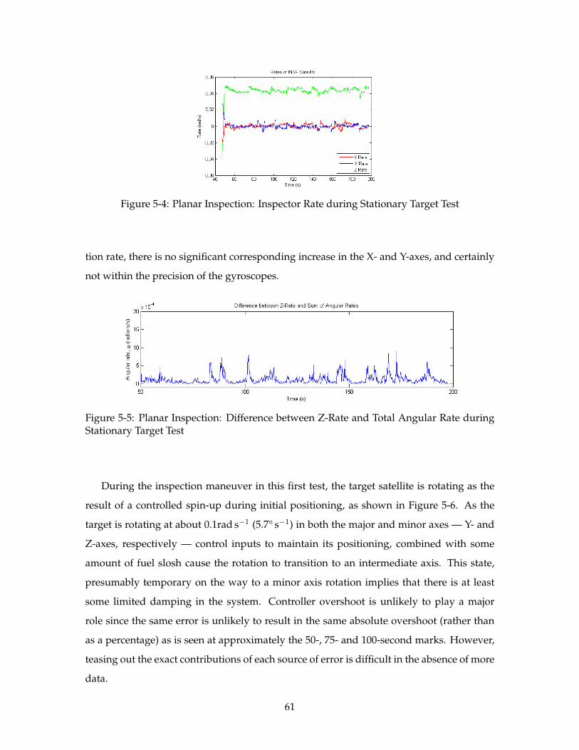
Figure 5-4: Planar Inspection: Inspector Rate during Stationary Target Test
tion rate, there is no significant corresponding increase in the X- and Y-axes, and certainly
not within the precision of the gyroscopes.
Figure 5-5: Planar Inspection: Difference between Z-Rate and Total Angular Rate duringStationary Target Test
During the inspection maneuver in this first test, the target satellite is rotating as the
result of a controlled spin-up during initial positioning, as shown in Figure 5-6. As the
target is rotating at about 0.1rad s−1 (5.7° s−1) in both the major and minor axes — Y- and
Z-axes, respectively — control inputs to maintain its positioning, combined with some
amount of fuel slosh cause the rotation to transition to an intermediate axis. This state,
presumably temporary on the way to a minor axis rotation implies that there is at least
some limited damping in the system. Controller overshoot is unlikely to play a major
role since the same error is unlikely to result in the same absolute overshoot (rather than
as a percentage) as is seen at approximately the 50-, 75- and 100-second marks. However,
teasing out the exact contributions of each source of error is difficult in the absence of more
data.
61
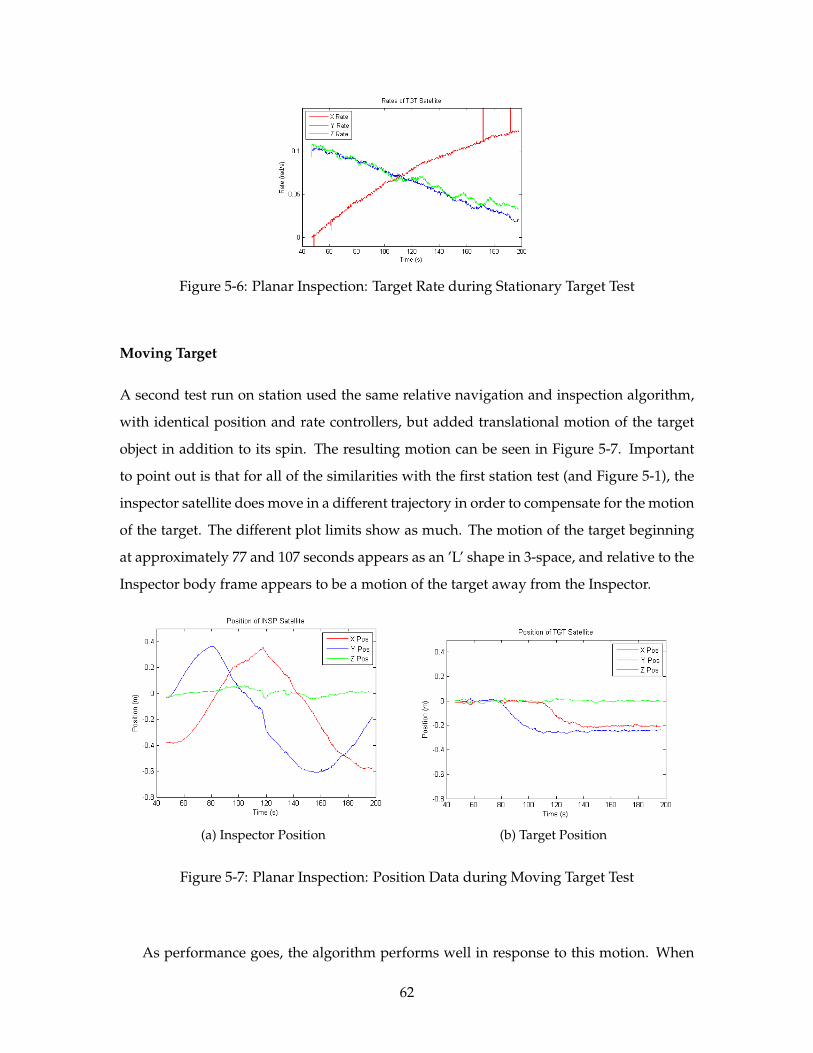
Figure 5-6: Planar Inspection: Target Rate during Stationary Target Test
Moving Target
A second test run on station used the same relative navigation and inspection algorithm,
with identical position and rate controllers, but added translational motion of the target
object in addition to its spin. The resulting motion can be seen in Figure 5-7. Important
to point out is that for all of the similarities with the first station test (and Figure 5-1), the
inspector satellite does move in a different trajectory in order to compensate for the motion
of the target. The different plot limits show as much. The motion of the target beginning
at approximately 77 and 107 seconds appears as an ’L’ shape in 3-space, and relative to the
Inspector body frame appears to be a motion of the target away from the Inspector.
(a) Inspector Position (b) Target Position
Figure 5-7: Planar Inspection: Position Data during Moving Target Test
As performance goes, the algorithm performs well in response to this motion. When
62
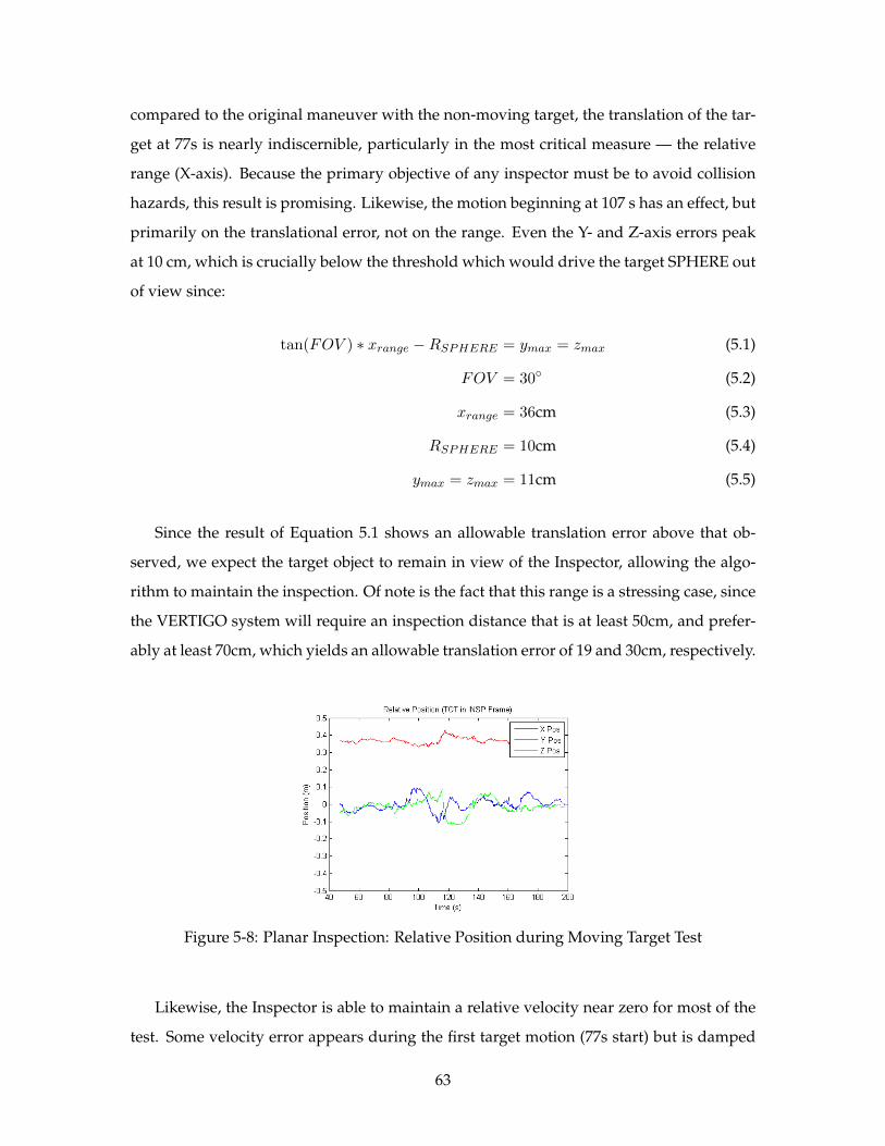
compared to the original maneuver with the non-moving target, the translation of the tar-
get at 77s is nearly indiscernible, particularly in the most critical measure — the relative
range (X-axis). Because the primary objective of any inspector must be to avoid collision
hazards, this result is promising. Likewise, the motion beginning at 107 s has an effect, but
primarily on the translational error, not on the range. Even the Y- and Z-axis errors peak
at 10 cm, which is crucially below the threshold which would drive the target SPHERE out
of view since:
tan(FOV ) ∗ xrange −RSPHERE = ymax = zmax (5.1)
FOV = 30◦ (5.2)
xrange = 36cm (5.3)
RSPHERE = 10cm (5.4)
ymax = zmax = 11cm (5.5)
Since the result of Equation 5.1 shows an allowable translation error above that ob-
served, we expect the target object to remain in view of the Inspector, allowing the algo-
rithm to maintain the inspection. Of note is the fact that this range is a stressing case, since
the VERTIGO system will require an inspection distance that is at least 50cm, and prefer-
ably at least 70cm, which yields an allowable translation error of 19 and 30cm, respectively.
Figure 5-8: Planar Inspection: Relative Position during Moving Target Test
Likewise, the Inspector is able to maintain a relative velocity near zero for most of the
test. Some velocity error appears during the first target motion (77s start) but is damped
63
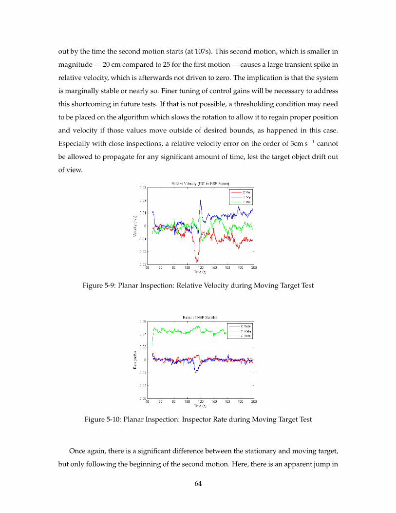
out by the time the second motion starts (at 107s). This second motion, which is smaller in
magnitude — 20 cm compared to 25 for the first motion — causes a large transient spike in
relative velocity, which is afterwards not driven to zero. The implication is that the system
is marginally stable or nearly so. Finer tuning of control gains will be necessary to address
this shortcoming in future tests. If that is not possible, a thresholding condition may need
to be placed on the algorithm which slows the rotation to allow it to regain proper position
and velocity if those values move outside of desired bounds, as happened in this case.
Especially with close inspections, a relative velocity error on the order of 3cm s−1 cannot
be allowed to propagate for any significant amount of time, lest the target object drift out
of view.
Figure 5-9: Planar Inspection: Relative Velocity during Moving Target Test
Figure 5-10: Planar Inspection: Inspector Rate during Moving Target Test
Once again, there is a significant difference between the stationary and moving target,
but only following the beginning of the second motion. Here, there is an apparent jump in
64
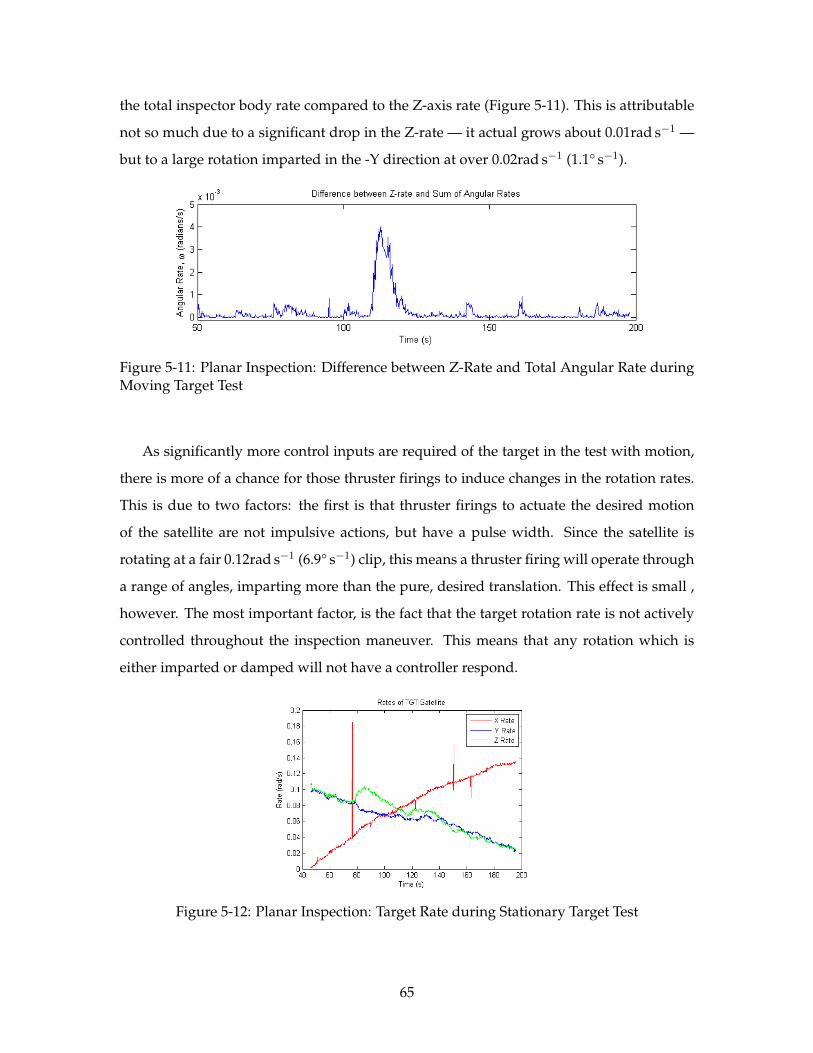
the total inspector body rate compared to the Z-axis rate (Figure 5-11). This is attributable
not so much due to a significant drop in the Z-rate — it actual grows about 0.01rad s−1 —
but to a large rotation imparted in the -Y direction at over 0.02rad s−1 (1.1° s−1).
Figure 5-11: Planar Inspection: Difference between Z-Rate and Total Angular Rate duringMoving Target Test
As significantly more control inputs are required of the target in the test with motion,
there is more of a chance for those thruster firings to induce changes in the rotation rates.
This is due to two factors: the first is that thruster firings to actuate the desired motion
of the satellite are not impulsive actions, but have a pulse width. Since the satellite is
rotating at a fair 0.12rad s−1 (6.9° s−1) clip, this means a thruster firing will operate through
a range of angles, imparting more than the pure, desired translation. This effect is small ,
however. The most important factor, is the fact that the target rotation rate is not actively
controlled throughout the inspection maneuver. This means that any rotation which is
either imparted or damped will not have a controller respond.
Figure 5-12: Planar Inspection: Target Rate during Stationary Target Test
65
5.1.2 Simulation Results
Prior to running the planar inspection maneuvers on the Space Station, they were com-
posed and tested in a Matlab simulation environment. This simulation, available for all
researchers working on the SPHERES system, allows the testing of code prior to launch. It
mimics the dynamics of the satellites along with thruster misalignment and non-linearities
(including hysteresis and deadband) and metrology system noise, among other factors,
which provide a good estimate of potential disturbances from an ideal system. A simula-
tion mode is also available which ignores sensor and thruster noise.
Stationary Target
The first maneuver with a stationary central target was run in the simulation. Figure 5-13
shows the inertial (ISS-relative) positions of the Inspector and target satellites. Here there is
good tracking of the desired positions, with circular motion easily visible in the left image.
Also noticeable is the fact that at the beginning of the inspection there is some small error in
initial positioning with the relative range (Figure 5-14) being off by 2cm and Y-position off
by approximately twice that amount This is the result of initial positioning taking longer
than the 30s allotted. This is not particularly significant as the error is small and even
when compounded by the initial angular acceleration to achieve the desired rotation rate,
the error is removed by the controller after 40s.
Even after removing the initial error, there is still a consistent error in the relative posi-
tion. Since the desired steady state condition is <36, 0, 0> cm in <X,Y,Z>, but the actual
state value approaches<38, 0, 0> there is clearly a steady state error in the controller used,
at least when a rotation is also commanded. Since the controller is PD on position, the po-
sition error is proportional to the control output. As it is implemented on SPHERES (and
therefore in the simulation), it is likely that the deadband eliminates the small thruster
forces associated with a 2cm error. A 10ms minimum firing time along with the steady
disturbance associated with the rotation causes the error to stay fixed near 2cm. The ad-
dition of an integral term would likely resolve this issue, but at the risk of increasing the
probability of the Inspector and target colliding. Such a decision should be made based on
the mission at hand and the risk tolerance of that mission profile and the system operators.
66
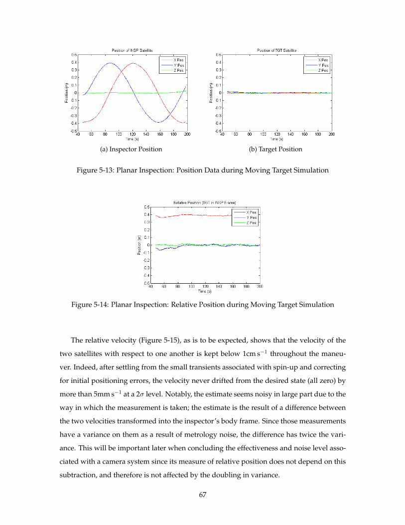
(a) Inspector Position (b) Target Position
Figure 5-13: Planar Inspection: Position Data during Moving Target Simulation
Figure 5-14: Planar Inspection: Relative Position during Moving Target Simulation
The relative velocity (Figure 5-15), as is to be expected, shows that the velocity of the
two satellites with respect to one another is kept below 1cm s−1 throughout the maneu-
ver. Indeed, after settling from the small transients associated with spin-up and correcting
for initial positioning errors, the velocity never drifted from the desired state (all zero) by
more than 5mm s−1 at a 2σ level. Notably, the estimate seems noisy in large part due to the
way in which the measurement is taken; the estimate is the result of a difference between
the two velocities transformed into the inspector’s body frame. Since those measurements
have a variance on them as a result of metrology noise, the difference has twice the vari-
ance. This will be important later when concluding the effectiveness and noise level asso-
ciated with a camera system since its measure of relative position does not depend on this
subtraction, and therefore is not affected by the doubling in variance.
67
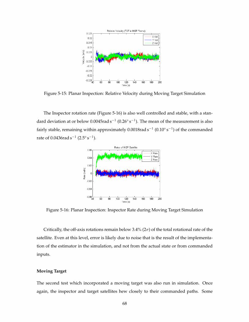
Figure 5-15: Planar Inspection: Relative Velocity during Moving Target Simulation
The Inspector rotation rate (Figure 5-16) is also well controlled and stable, with a stan-
dard deviation at or below 0.0045rad s−1 (0.26° s−1). The mean of the measurement is also
fairly stable, remaining within approximately 0.0018rad s−1 (0.10° s−1) of the commanded
rate of 0.0436rad s−1 (2.5° s−1).
Figure 5-16: Planar Inspection: Inspector Rate during Moving Target Simulation
Critically, the off-axis rotations remain below 3.4% (2σ) of the total rotational rate of the
satellite. Even at this level, error is likely due to noise that is the result of the implementa-
tion of the estimator in the simulation, and not from the actual state or from commanded
inputs.
Moving Target
The second test which incorporated a moving target was also run in simulation. Once
again, the inspector and target satellites hew closely to their commanded paths. Some
68
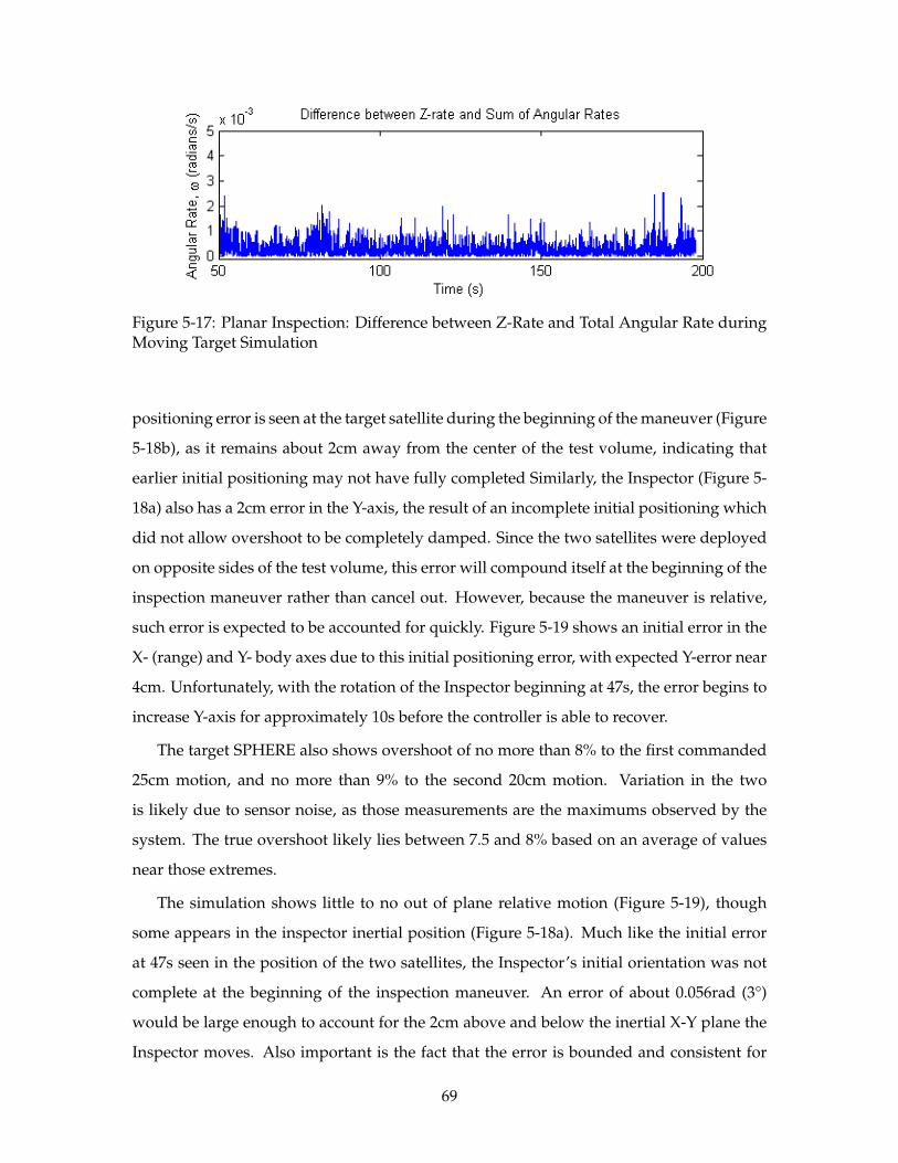
Figure 5-17: Planar Inspection: Difference between Z-Rate and Total Angular Rate duringMoving Target Simulation
positioning error is seen at the target satellite during the beginning of the maneuver (Figure
5-18b), as it remains about 2cm away from the center of the test volume, indicating that
earlier initial positioning may not have fully completed Similarly, the Inspector (Figure 5-
18a) also has a 2cm error in the Y-axis, the result of an incomplete initial positioning which
did not allow overshoot to be completely damped. Since the two satellites were deployed
on opposite sides of the test volume, this error will compound itself at the beginning of the
inspection maneuver rather than cancel out. However, because the maneuver is relative,
such error is expected to be accounted for quickly. Figure 5-19 shows an initial error in the
X- (range) and Y- body axes due to this initial positioning error, with expected Y-error near
4cm. Unfortunately, with the rotation of the Inspector beginning at 47s, the error begins to
increase Y-axis for approximately 10s before the controller is able to recover.
The target SPHERE also shows overshoot of no more than 8% to the first commanded
25cm motion, and no more than 9% to the second 20cm motion. Variation in the two
is likely due to sensor noise, as those measurements are the maximums observed by the
system. The true overshoot likely lies between 7.5 and 8% based on an average of values
near those extremes.
The simulation shows little to no out of plane relative motion (Figure 5-19), though
some appears in the inspector inertial position (Figure 5-18a). Much like the initial error
at 47s seen in the position of the two satellites, the Inspector’s initial orientation was not
complete at the beginning of the inspection maneuver. An error of about 0.056rad (3°)
would be large enough to account for the 2cm above and below the inertial X-Y plane the
Inspector moves. Also important is the fact that the error is bounded and consistent for
69
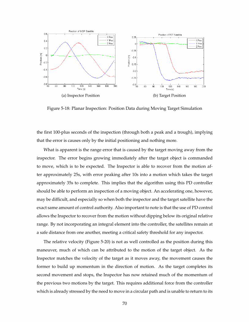
(a) Inspector Position (b) Target Position
Figure 5-18: Planar Inspection: Position Data during Moving Target Simulation
the first 100-plus seconds of the inspection (through both a peak and a trough), implying
that the error is causes only by the initial positioning and nothing more.
What is apparent is the range error that is caused by the target moving away from the
inspector. The error begins growing immediately after the target object is commanded
to move, which is to be expected. The Inspector is able to recover from the motion af-
ter approximately 25s, with error peaking after 10s into a motion which takes the target
approximately 35s to complete. This implies that the algorithm using this PD controller
should be able to perform an inspection of a moving object. An accelerating one, however,
may be difficult, and especially so when both the inspector and the target satellite have the
exact same amount of control authority. Also important to note is that the use of PD control
allows the Inspector to recover from the motion without dipping below its original relative
range. By not incorporating an integral element into the controller, the satellites remain at
a safe distance from one another, meeting a critical safety threshold for any inspector.
The relative velocity (Figure 5-20) is not as well controlled as the position during this
maneuver, much of which can be attributed to the motion of the target object. As the
Inspector matches the velocity of the target as it moves away, the movement causes the
former to build up momentum in the direction of motion. As the target completes its
second movement and stops, the Inspector has now retained much of the momentum of
the previous two motions by the target. This requires additional force from the controller
which is already stressed by the need to move in a circular path and is unable to return to its
70
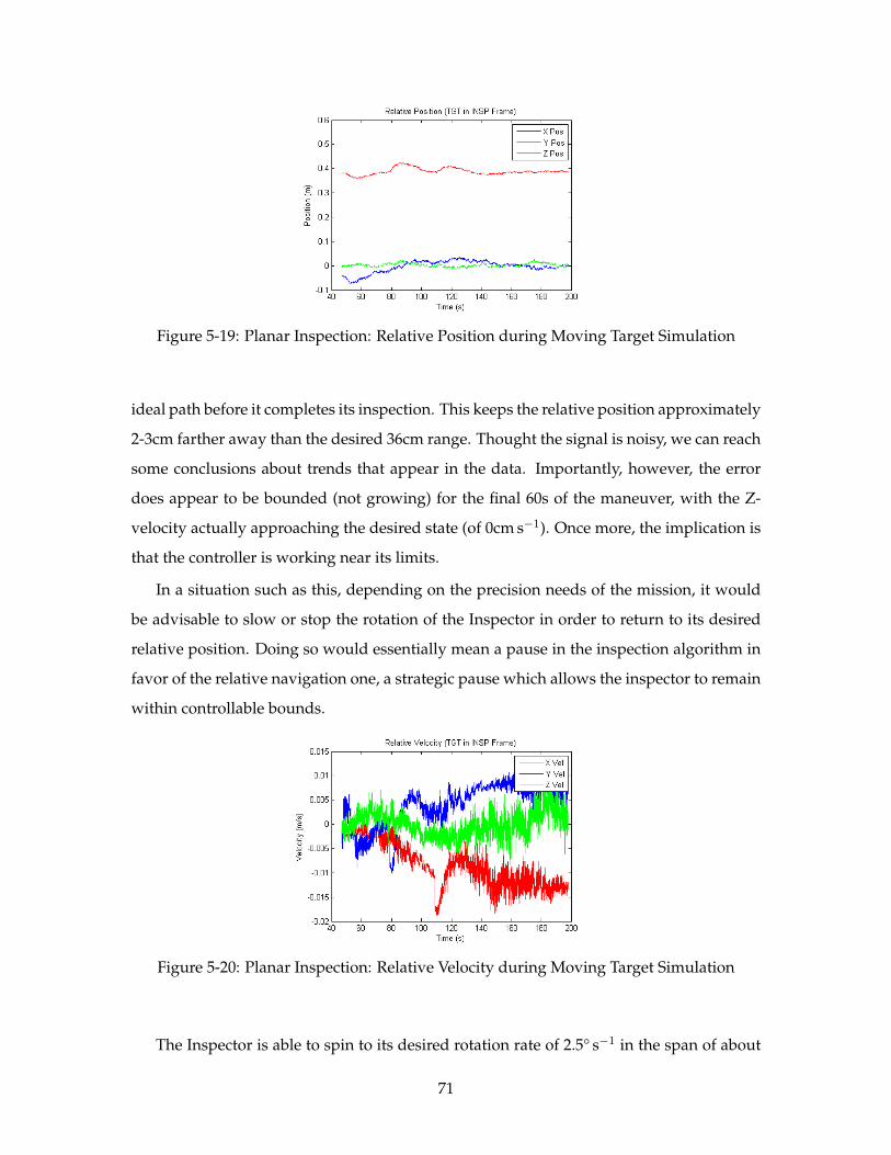
Figure 5-19: Planar Inspection: Relative Position during Moving Target Simulation
ideal path before it completes its inspection. This keeps the relative position approximately
2-3cm farther away than the desired 36cm range. Thought the signal is noisy, we can reach
some conclusions about trends that appear in the data. Importantly, however, the error
does appear to be bounded (not growing) for the final 60s of the maneuver, with the Z-
velocity actually approaching the desired state (of 0cm s−1). Once more, the implication is
that the controller is working near its limits.
In a situation such as this, depending on the precision needs of the mission, it would
be advisable to slow or stop the rotation of the Inspector in order to return to its desired
relative position. Doing so would essentially mean a pause in the inspection algorithm in
favor of the relative navigation one, a strategic pause which allows the inspector to remain
within controllable bounds.
Figure 5-20: Planar Inspection: Relative Velocity during Moving Target Simulation
The Inspector is able to spin to its desired rotation rate of 2.5° s−1 in the span of about
71
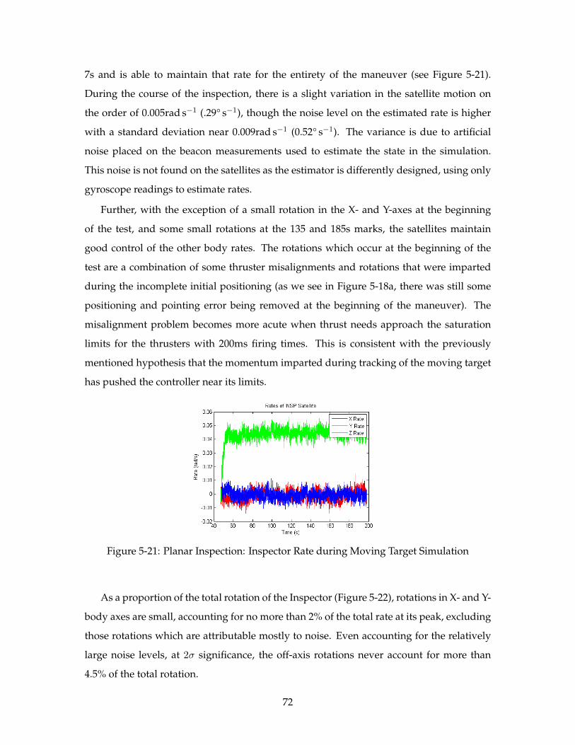
7s and is able to maintain that rate for the entirety of the maneuver (see Figure 5-21).
During the course of the inspection, there is a slight variation in the satellite motion on
the order of 0.005rad s−1 (.29° s−1), though the noise level on the estimated rate is higher
with a standard deviation near 0.009rad s−1 (0.52° s−1). The variance is due to artificial
noise placed on the beacon measurements used to estimate the state in the simulation.
This noise is not found on the satellites as the estimator is differently designed, using only
gyroscope readings to estimate rates.
Further, with the exception of a small rotation in the X- and Y-axes at the beginning
of the test, and some small rotations at the 135 and 185s marks, the satellites maintain
good control of the other body rates. The rotations which occur at the beginning of the
test are a combination of some thruster misalignments and rotations that were imparted
during the incomplete initial positioning (as we see in Figure 5-18a, there was still some
positioning and pointing error being removed at the beginning of the maneuver). The
misalignment problem becomes more acute when thrust needs approach the saturation
limits for the thrusters with 200ms firing times. This is consistent with the previously
mentioned hypothesis that the momentum imparted during tracking of the moving target
has pushed the controller near its limits.
Figure 5-21: Planar Inspection: Inspector Rate during Moving Target Simulation
As a proportion of the total rotation of the Inspector (Figure 5-22), rotations in X- and Y-
body axes are small, accounting for no more than 2% of the total rate at its peak, excluding
those rotations which are attributable mostly to noise. Even accounting for the relatively
large noise levels, at 2σ significance, the off-axis rotations never account for more than
4.5% of the total rotation.
72
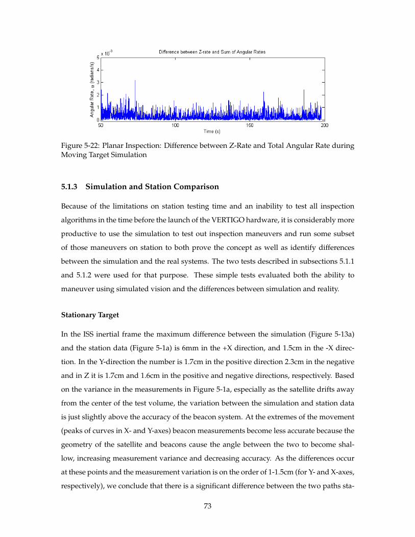
Figure 5-22: Planar Inspection: Difference between Z-Rate and Total Angular Rate duringMoving Target Simulation
5.1.3 Simulation and Station Comparison
Because of the limitations on station testing time and an inability to test all inspection
algorithms in the time before the launch of the VERTIGO hardware, it is considerably more
productive to use the simulation to test out inspection maneuvers and run some subset
of those maneuvers on station to both prove the concept as well as identify differences
between the simulation and the real systems. The two tests described in subsections 5.1.1
and 5.1.2 were used for that purpose. These simple tests evaluated both the ability to
maneuver using simulated vision and the differences between simulation and reality.
Stationary Target
In the ISS inertial frame the maximum difference between the simulation (Figure 5-13a)
and the station data (Figure 5-1a) is 6mm in the +X direction, and 1.5cm in the -X direc-
tion. In the Y-direction the number is 1.7cm in the positive direction 2.3cm in the negative
and in Z it is 1.7cm and 1.6cm in the positive and negative directions, respectively. Based
on the variance in the measurements in Figure 5-1a, especially as the satellite drifts away
from the center of the test volume, the variation between the simulation and station data
is just slightly above the accuracy of the beacon system. At the extremes of the movement
(peaks of curves in X- and Y-axes) beacon measurements become less accurate because the
geometry of the satellite and beacons cause the angle between the two to become shal-
low, increasing measurement variance and decreasing accuracy. As the differences occur
at these points and the measurement variation is on the order of 1-1.5cm (for Y- and X-axes,
respectively), we conclude that there is a significant difference between the two paths sta-
73
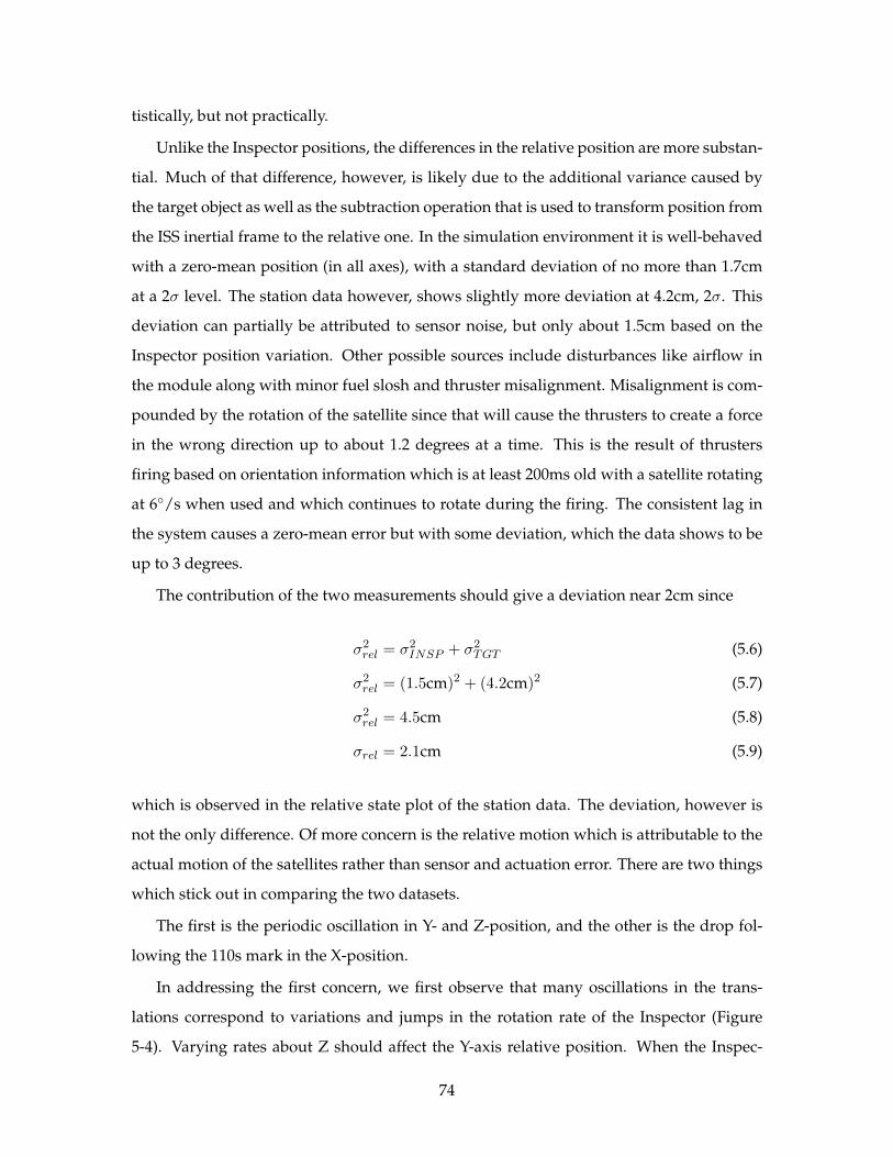
tistically, but not practically.
Unlike the Inspector positions, the differences in the relative position are more substan-
tial. Much of that difference, however, is likely due to the additional variance caused by
the target object as well as the subtraction operation that is used to transform position from
the ISS inertial frame to the relative one. In the simulation environment it is well-behaved
with a zero-mean position (in all axes), with a standard deviation of no more than 1.7cm
at a 2σ level. The station data however, shows slightly more deviation at 4.2cm, 2σ. This
deviation can partially be attributed to sensor noise, but only about 1.5cm based on the
Inspector position variation. Other possible sources include disturbances like airflow in
the module along with minor fuel slosh and thruster misalignment. Misalignment is com-
pounded by the rotation of the satellite since that will cause the thrusters to create a force
in the wrong direction up to about 1.2 degrees at a time. This is the result of thrusters
firing based on orientation information which is at least 200ms old with a satellite rotating
at 6◦/s when used and which continues to rotate during the firing. The consistent lag in
the system causes a zero-mean error but with some deviation, which the data shows to be
up to 3 degrees.
The contribution of the two measurements should give a deviation near 2cm since
σ2rel = σ2INSP + σ2TGT (5.6)
σ2rel = (1.5cm)2 + (4.2cm)2 (5.7)
σ2rel = 4.5cm (5.8)
σrel = 2.1cm (5.9)
which is observed in the relative state plot of the station data. The deviation, however is
not the only difference. Of more concern is the relative motion which is attributable to the
actual motion of the satellites rather than sensor and actuation error. There are two things
which stick out in comparing the two datasets.
The first is the periodic oscillation in Y- and Z-position, and the other is the drop fol-
lowing the 110s mark in the X-position.
In addressing the first concern, we first observe that many oscillations in the trans-
lations correspond to variations and jumps in the rotation rate of the Inspector (Figure
5-4). Varying rates about Z should affect the Y-axis relative position. When the Inspec-
74
tor increases its rotation rate quickly, system lag causes the horizontal (Y-axis) component
to grow, pushing the Y-relative position positive until the position controller is able to
catch up to the new rotation rate. Furthermore, the design of the controller may be lightly
damped in the presence of disturbances. Fine-tuning of the controller gains for future
development efforts would solve this problem. That said, with the current design, it is
expected that there may be error in the Y- and Z- directions up to approximately 5cm and
has the same period as the jumps in rotational velocity.
To address the second, it is important to refer back to the inertial position of the In-
spector satellite (Figure 5-1a). That measurement ha s similar drop of nearly 4cm over the
period of 200ms. Therefore, this drop is likely an artifact the metrology system, possibly
due to a bad ultrasound reading that the internal state estimator (an EKF) is not able to
completely disregard and which then persists in the state estimate for the next 4-5s. Such
outliers are possible with the vision system, but since the implementation of the controller
with the vision system does not currently filter its data, outliers will be transient events
that do not effect the position controller beyond the current frame. Future vision estima-
tors and outlier detection that should be included on the vision system can be tuned to
eliminate the occasional large jumps like what is seen in Figure 5-1a large jumps.
From these two differences we make the following two claims about the differences
between simulation and ISS tests:
1. Y-/Z-axis errors are linked to variations in the rotation rate.
2. At a range of 36cm, variations are up to 5cm in Y/Z.
Since the position errors are so closely coupled with the rotation rates, it is those rates
which we shall next examine. Referring back to Figure 5-4, we observe that the Z-rate
has a 2σ deviation of 6.7mrad s−1 (0.39° s−1) about the commanded mean of 0.0436rad s−1
(2.5° s−1). The X- and Y-rates have a similar distribution, but around a commanded mean
which is instead zero.
The peaks in the Z body rate come approximately every 20-21s. This is likely the result
of large thruster inputs that is the result of a fairly wide deadband in the controller that
comes from the relatively small control gain that is placed on the angular rate. Coupled
with the dynamics associated with rotation about a minor moment of inertia, this causes
the rotation to reach a peak slightly above the desired rate, then decay (as is visible in the
75
target rate decay in Figure 5-6) until the controller can once again provide enough control
authority for another thruster firing.
Unlike the simulation, however, the rate has far less noise on the measurement as a
result of the different measurements used in the simulation and in the SPHERES stan-
dard estimator. Since the standard estimator uses the gyroscope measurements as truth,
the variation in the rotation measurements is equivalent to the sum of the movement of
the satellite itself and the noise of the measurements. An estimate of the variation which
subtracts the variation due to the satellite motion (itself an estimate of the decay of the
satellite rate) yields a standard deviation around 1.395mrad s−1 (0.080° s−1) at a 1σ signif-
icance. That estimate, using the data from the first 50s of the maneuver, is liable to drift
over the course of the test. However, with random noise in that range, the angular random
walk is expected to be about 7.66mrad (0.44°) after a 150s maneuver. The random walk is
derived as follows[35]:
σARW = σgyro√
∆T ∗ Ttotal (5.10)
σgyro = 0.080◦/s (5.11)
Ttotal = 150.4s (5.12)
∆T = 0.2s/measurement (5.13)
σARW = (0.080◦/s)√
(0.2s) ∗ (150.4s) (5.14)
σARW = 0.44◦ (5.15)
These results actually exceed the specification sheet for the gyroscopes, which give a
resolution of 0.0407° s−1, with a noise ceiling of 0.05, which works out to a 1-σ error up to
0.35 ° s−1 at 50Hz[36].
Prior to moving onto an analysis of the inspection with motion it is important to note
a few remaining items about the gyroscope measurements based on the target object’s
rotation estimate. The first is that the standard deviation approaches the same value with
a sample showing approximately 1.42mrad s−1 (0.081° s−1) of standard deviation at 1σ
significance. This level is exceptionally close — within 1.3% — to the estimate given by the
Inspector satellite, providing another check on the value. The second is that the somewhere
along the line the gyroscopes will occasionally provide outliers, particularly in the X-axis
76
of the target satellite. Over the course of a 150s maneuver, there were 3 exceptionally
significant outliers (100s of % error) and a fourth which is still significant error (at 60%
deviation from the immediately preceding and following measurements). Though these
errors did not cause any significant problem during the course of the inspection since the
rotation of the target was not actively controlled, it may be worthwhile to avoid using the
satellite used as the target in this test as an inspector in future operations.
Moving Target
Once the target adds motion the path in inertial space matches up well with the simulation,
even better perhaps, than in the previous test with a stationary target. The overshoot of
the target satellite was approximately 3% in the inertial frame (Figure 5-7b vs 5-18b).
Station results from the Inspector’s inertial position (Figure 5-7a) also track well with
the simulation data (Figure 5-18a). With the exception of the maximum observed in the X-
axis, all other peaks (X-min, Y-max and Y-min) occur within 1s of the predicted time. The
exception occurs 5s later, though that may be the result of noise on the metrology system.
The overall error in those same peaks is 1.6% for an average of 7.7mm error in positioning.
The relative position is more important than the inertial one, however. Refer back
to Figures 5-8 and 5-19. In those plots, as well as the supporting data, we observe that
there is significantly more noise and variation on the relative positions when compared to
an inspection with a nearly static target object (Figure 5-2). Control in the X-axis (range)
actually maintains itself fairly well with error staying within approximately [-3,7]cm of
the desired 36cm range. Much of that error in the negative direction is cause by lag in the
controller as it tries to bleed momentum acquired by matching the target object’s speed. In
the positive direction, the adjustments being made by the controller in order to deal with
the slowing target work against the Inspector as the target then begins motion away once
more.
Compared with the simulation, the general shape of the Inspection matches well —
there are peaks near 85 and 120s as the Inspector reaches its maximum distance from the
target, as well as a trough near 107s as the second motion begins. The timing agrees well,
but it is the magnitude of these which is incorrectly estimated in the simulation. Relative to
the commanded position of 36cm, the peaks and troughs exceed this in simulation by 6.3,
2.8, and 4.9cm, while the actual data shows errors of 2.9, -3.1, and 7.0cm. The implication
77
for future tests is therefore the following:
1. The actual system maintains an average range to target better than predicted in sim-
ulation by up to 2cm, or 6%.
2. A single target motion in simulation which causes up to 1.7cm in error may cause up
to 3cm in hardware, or roughly double.
3. A second motion will cause error to compound, creating a peak up to 2.5 times larger,
where simulation may predict no growth in error relative to previous motions.
Examining the Y- and Z-axis errors, we observe that both simulation and station data
shows that it is zero-mean but that the magnitude of that error is much higher when run
on that hardware. This, however, appears to be the result of poor control in the angular
rate of the satellite rather than the position controller itself (see Figure 5-10). This is also
partially to blame for the error in the Inspector’s body X-axis. This allows the error to
change by 20cm in the span of 4s, as does somewhat noisy position relative position data
that sees very large variation throughout the test and does so at a rate that the satellite
cannot achieve by translation alone.
The conclusions that may be drawn from the data is this:
1. There is no bias in the simulation with Y- and Z-axis positions.
2. Pointing and metrology errors causes the error in these axes to be approximately
twice what is predicted in simulation (5cm in simulation, 10 on station).
To close out the comparison, we next examine the rates of the Inspector satellite. As
with the inspection with no target motion, we see significantly less noise in the station
data (Figure 5-10) than with the simulation (Figure 5-21). This has the same cause, which
is the different methods used to estimate the rate — the simulation uses the beacons and
their attendant noise where the satellites themselves use their more accurate gyroscopes
for measurements. The error in measured vs. commanded rates is zero mean, but the sim-
ulation noise is on the order of 0.01rad s−1 (0.57° s−1), where the real data shows variation
no greater than half of that, at 0.005rad s−1 (0.29° s−1). While the noise is much lower than
in simulation, and the X- and Y-rates match well, there are some differences which are
less beneficial. When the controller is stressed, as is the case following the second motion
78
of the target, rate errors may grow to 0.018rad s−1 (1.0° s−1) in off-axis rotations, though
only 3.9mrad s−1 (0.22° s−1) in the Z-direction. In less than 10s, however, those errors are
expected to damp out.
Critically, the most important fundamental difference between the simulation and the
station data is damping in the system which causes rotation about the minor axis to slow
consistently until thruster activity respins the satellite and controls rotation in the off axes.
This damping, which is uncontrolled in the target (Figure 5-12), would cause the rotational
axes to slowly change over the course of an inspection if left alone. This means that for a
successful maneuver the rotation of the Inspector must be closed loop rather than the initial
spin up that is used for the target.
Ultimately, these data points allows us to draw the following conclusions:
1. Simulation and station rate data show error that is zero mean, but the standard de-
viation of the simulation is double what is to be expected on station.
2. Damping is present on station that is not accounted for in simulation.
5.1.4 Simulation Only
The previous two subsections described tests which were run on the International Space
Station following simulations which demonstrated their ability to control an Inspector per-
forms a circumnavigation of a target object. The targets also demonstrated that the ma-
neuver is robust to limited movement by the target object. Based on the comparison of the
predicted and actual maneuver performances, we may analyze four additional tests that
were developed and run in simulation. Those tests are (the code for which is included in
Appendix A.2):
1. Additional Motion This test is a continuation of the motion test that was run on
station, but with movement perpendicular to the inspection plane as well as motion
of the target toward the Inspector.
2. 3D Inspection This test finally moves out of the planar inspection and attempts to
get full coverage of the target object.
3. Long Duration Planar Inspection This inspection is identical to the first, stationary
target test, save for a duration of 10 minutes rather than 4. This is done for two
79
purposes: on station this would allow a better characterization of gyroscope drift
while in simulation it potentially allows for greater coverage while remaining in a
planar motion.
4. Inclusion of Rotation Information The final test uses rotation information in order
to build a more fuel- and time-efficient inspection path, as it takes measurements of
the rotation rate of the target satellite in order to estimate its own coverage perfor-
mance.
Further, each of these tests is designed to be run at 70cm range rather than 36cm. While
this makes it more difficult for the inspection to fit within the space station test volume,
it more closely fits the range at which the VERTIGO system is designed to operate. To
compensate for the additional distance that needed to be travelled for a similar angular
rotation, the satellite rotation rate was dropped from 2.5 to 1.5° s−1.
Additional Motion
In this test, we aim to determine the reaction of the Inspector satellite to motion by the
target, but rather than having the target satellite move away, a la the second station test, it
will move toward the Inspector, and then in a shear direction to it. During this test we aim
to characterize the motion by determining the closest approach, overshoot, and stability.
The primary objective will be to quantify these values in the relative frame, though looking
at the inertial frame is also useful, especially for visualizing the motion.
For this test, the satellites begin slightly offset from the center of the volume in order to
ensure that there is sufficient room for maneuvering. At the 60s mark in this maneuver, the
target moves first in the Y-direction toward the Inspector. 60s later, the satellite moves once
more, this time in the negative Z-direction. In both cases, the Inspector adjusts, chasing its
target. Figure 5-23a shows the former’s motion, while Figure 5-23b shows the latter.
The simulation shows the motion is well controlled. The overshoot of the target satellite
is at or below 10% for the both motions. The more interesting motion, however, is that of
the Inspector. In this maneuver, the Inspector begins to react to the motion of the target
within 2s in both directions. Such a reaction matches fairly well with what was observed
in the station tests. What differs, however, is the Z-location of the Inspector, which appears
to have set up a periodic motion. This change is not easily detectable in the gyros because
80

(a) Inspector Position (b) Target Position
Figure 5-23: Planar Inspection: Position Data during “Additional Motion” Simulation
of the simulation noise (see Figure 5-25), but a cursory examination suggests that this is
caused by a misalignment that happens during the vertical motion that is maintained.
This can probably be attributed to thruster simulated misalignment, as a similar angular
error is seen during initial positioning (not plotted).
Nevertheless, the inspection does maintain the proper distance, never approaching
closer than 68cm on the desired 70cm range (see Figure 5-24). This minimum comes 5s
after the motion of the target toward the inspector begins. On the whole, proper distance
is maintained within a centimeter of the commanded range excluding the peak due to the
motion.
Figure 5-24: Planar Inspection: Relative Position during “Additional Motion” Simulation
81
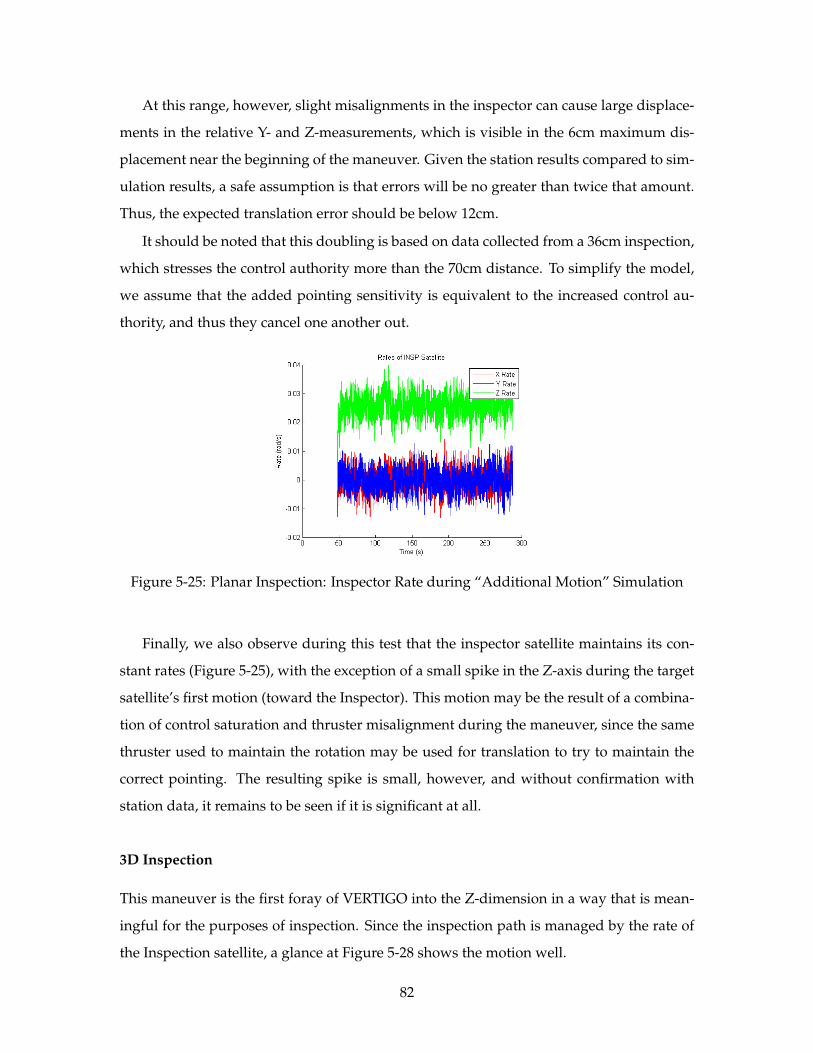
At this range, however, slight misalignments in the inspector can cause large displace-
ments in the relative Y- and Z-measurements, which is visible in the 6cm maximum dis-
placement near the beginning of the maneuver. Given the station results compared to sim-
ulation results, a safe assumption is that errors will be no greater than twice that amount.
Thus, the expected translation error should be below 12cm.
It should be noted that this doubling is based on data collected from a 36cm inspection,
which stresses the control authority more than the 70cm distance. To simplify the model,
we assume that the added pointing sensitivity is equivalent to the increased control au-
thority, and thus they cancel one another out.
Figure 5-25: Planar Inspection: Inspector Rate during “Additional Motion” Simulation
Finally, we also observe during this test that the inspector satellite maintains its con-
stant rates (Figure 5-25), with the exception of a small spike in the Z-axis during the target
satellite’s first motion (toward the Inspector). This motion may be the result of a combina-
tion of control saturation and thruster misalignment during the maneuver, since the same
thruster used to maintain the rotation may be used for translation to try to maintain the
correct pointing. The resulting spike is small, however, and without confirmation with
station data, it remains to be seen if it is significant at all.
3D Inspection
This maneuver is the first foray of VERTIGO into the Z-dimension in a way that is mean-
ingful for the purposes of inspection. Since the inspection path is managed by the rate of
the Inspection satellite, a glance at Figure 5-28 shows the motion well.
82
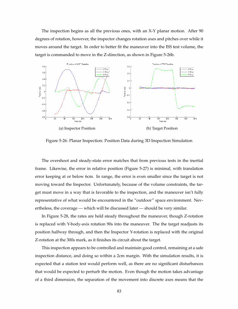
The inspection begins as all the previous ones, with an X-Y planar motion. After 90
degrees of rotation, however, the inspector changes rotation axes and pitches over while it
moves around the target. In order to better fit the maneuver into the ISS test volume, the
target is commanded to move in the Z-direction, as shown in Figure 5-26b.
(a) Inspector Position (b) Target Position
Figure 5-26: Planar Inspection: Position Data during 3D Inspection Simulation
The overshoot and steady-state error matches that from previous tests in the inertial
frame. Likewise, the error in relative position (Figure 5-27) is minimal, with translation
error keeping at or below 6cm. In range, the error is even smaller since the target is not
moving toward the Inspector. Unfortunately, because of the volume constraints, the tar-
get must move in a way that is favorable to the inspection, and the maneuver isn’t fully
representative of what would be encountered in the “outdoor” space environment. Nev-
ertheless, the coverage — which will be discussed later — should be very similar.
In Figure 5-28, the rates are held steady throughout the maneuver, though Z-rotation
is replaced with Y-body-axis rotation 90s into the maneuver. The the target readjusts its
position halfway through, and then the Inspector Y-rotation is replaced with the original
Z-rotation at the 300s mark, as it finishes its circuit about the target.
This inspection appears to be controlled and maintain good control, remaining at a safe
inspection distance, and doing so within a 2cm margin. With the simulation results, it is
expected that a station test would perform well, as there are no significant disturbances
that would be expected to perturb the motion. Even though the motion takes advantage
of a third dimension, the separation of the movement into discrete axes means that the
83
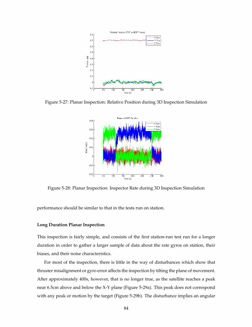
Figure 5-27: Planar Inspection: Relative Position during 3D Inspection Simulation
Figure 5-28: Planar Inspection: Inspector Rate during 3D Inspection Simulation
performance should be similar to that in the tests run on station.
Long Duration Planar Inspection
This inspection is fairly simple, and consists of the first station-run test run for a longer
duration in order to gather a larger sample of data about the rate gyros on station, their
biases, and their noise characteristics.
For most of the inspection, there is little in the way of disturbances which show that
thruster misalignment or gyro error affects the inspection by tilting the plane of movement.
After approximately 400s, however, that is no longer true, as the satellite reaches a peak
near 6.5cm above and below the X-Y plane (Figure 5-29a). This peak does not correspond
with any peak or motion by the target (Figure 5-29b). The disturbance implies an angular
84
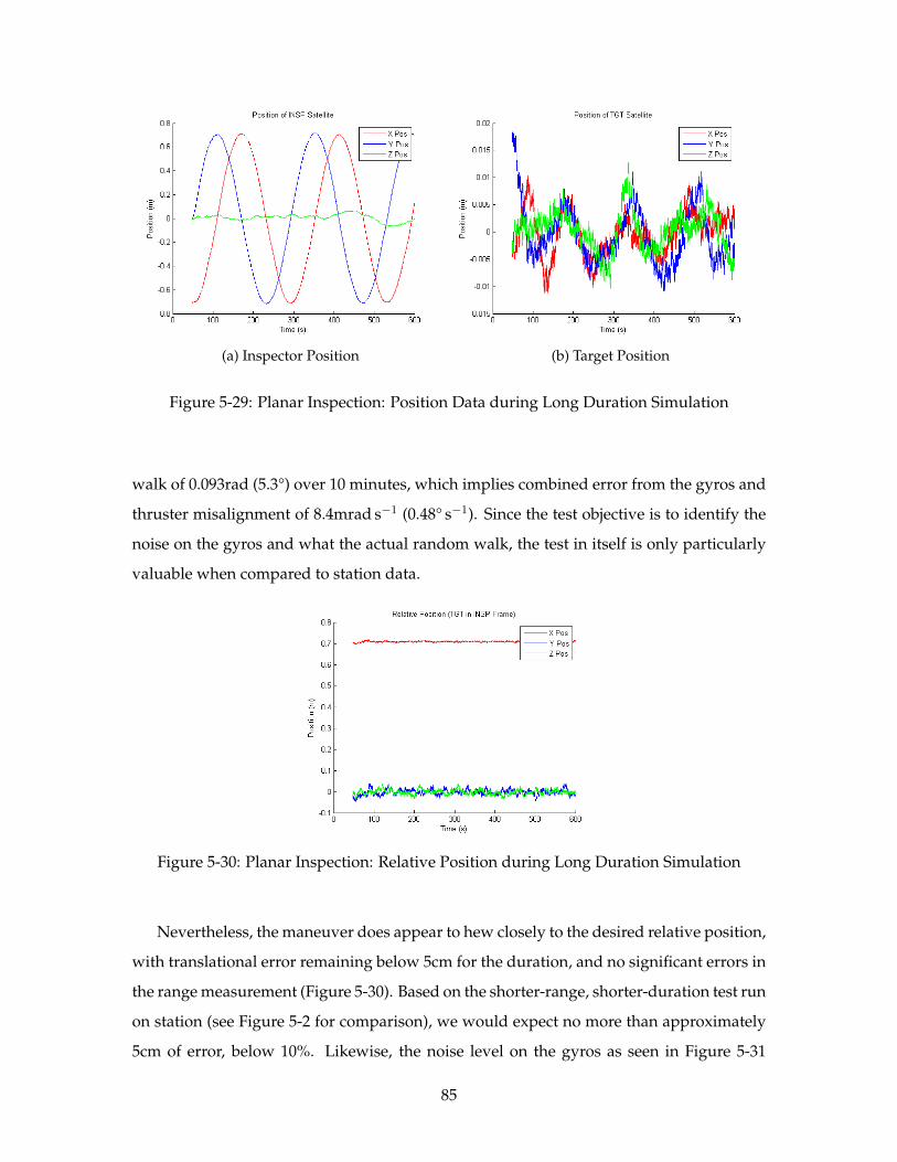
(a) Inspector Position (b) Target Position
Figure 5-29: Planar Inspection: Position Data during Long Duration Simulation
walk of 0.093rad (5.3°) over 10 minutes, which implies combined error from the gyros and
thruster misalignment of 8.4mrad s−1 (0.48° s−1). Since the test objective is to identify the
noise on the gyros and what the actual random walk, the test in itself is only particularly
valuable when compared to station data.
Figure 5-30: Planar Inspection: Relative Position during Long Duration Simulation
Nevertheless, the maneuver does appear to hew closely to the desired relative position,
with translational error remaining below 5cm for the duration, and no significant errors in
the range measurement (Figure 5-30). Based on the shorter-range, shorter-duration test run
on station (see Figure 5-2 for comparison), we would expect no more than approximately
5cm of error, below 10%. Likewise, the noise level on the gyros as seen in Figure 5-31
85
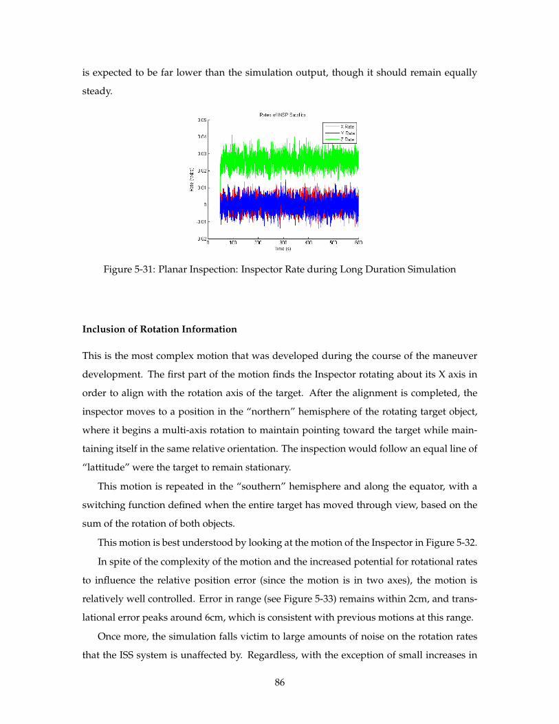
is expected to be far lower than the simulation output, though it should remain equally
steady.
Figure 5-31: Planar Inspection: Inspector Rate during Long Duration Simulation
Inclusion of Rotation Information
This is the most complex motion that was developed during the course of the maneuver
development. The first part of the motion finds the Inspector rotating about its X axis in
order to align with the rotation axis of the target. After the alignment is completed, the
inspector moves to a position in the “northern” hemisphere of the rotating target object,
where it begins a multi-axis rotation to maintain pointing toward the target while main-
taining itself in the same relative orientation. The inspection would follow an equal line of
“lattitude” were the target to remain stationary.
This motion is repeated in the “southern” hemisphere and along the equator, with a
switching function defined when the entire target has moved through view, based on the
sum of the rotation of both objects.
This motion is best understood by looking at the motion of the Inspector in Figure 5-32.
In spite of the complexity of the motion and the increased potential for rotational rates
to influence the relative position error (since the motion is in two axes), the motion is
relatively well controlled. Error in range (see Figure 5-33) remains within 2cm, and trans-
lational error peaks around 6cm, which is consistent with previous motions at this range.
Once more, the simulation falls victim to large amounts of noise on the rotation rates
that the ISS system is unaffected by. Regardless, with the exception of small increases in
86
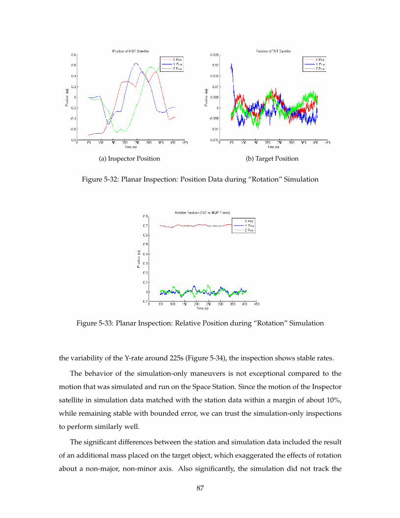
(a) Inspector Position (b) Target Position
Figure 5-32: Planar Inspection: Position Data during “Rotation” Simulation
Figure 5-33: Planar Inspection: Relative Position during “Rotation” Simulation
the variability of the Y-rate around 225s (Figure 5-34), the inspection shows stable rates.
The behavior of the simulation-only maneuvers is not exceptional compared to the
motion that was simulated and run on the Space Station. Since the motion of the Inspector
satellite in simulation data matched with the station data within a margin of about 10%,
while remaining stable with bounded error, we can trust the simulation-only inspections
to perform similarly well.
The significant differences between the station and simulation data included the result
of an additional mass placed on the target object, which exaggerated the effects of rotation
about a non-major, non-minor axis. Also significantly, the simulation did not track the
87
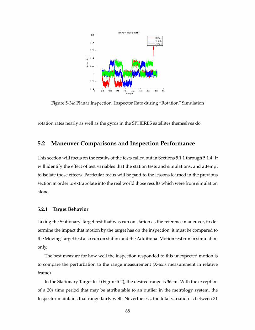
Figure 5-34: Planar Inspection: Inspector Rate during “Rotation” Simulation
rotation rates nearly as well as the gyros in the SPHERES satellites themselves do.
5.2 Maneuver Comparisons and Inspection Performance
This section will focus on the results of the tests called out in Sections 5.1.1 through 5.1.4. It
will identify the effect of test variables that the station tests and simulations, and attempt
to isolate those effects. Particular focus will be paid to the lessons learned in the previous
section in order to extrapolate into the real world those results which were from simulation
alone.
5.2.1 Target Behavior
Taking the Stationary Target test that was run on station as the reference maneuver, to de-
termine the impact that motion by the target has on the inspection, it must be compared to
the Moving Target test also run on station and the Additional Motion test run in simulation
only.
The best measure for how well the inspection responded to this unexpected motion is
to compare the perturbation to the range measurement (X-axis measurement in relative
frame).
In the Stationary Target test (Figure 5-2), the desired range is 36cm. With the exception
of a 20s time period that may be attributable to an outlier in the metrology system, the
Inspector maintains that range fairly well. Nevertheless, the total variation is between 31
88
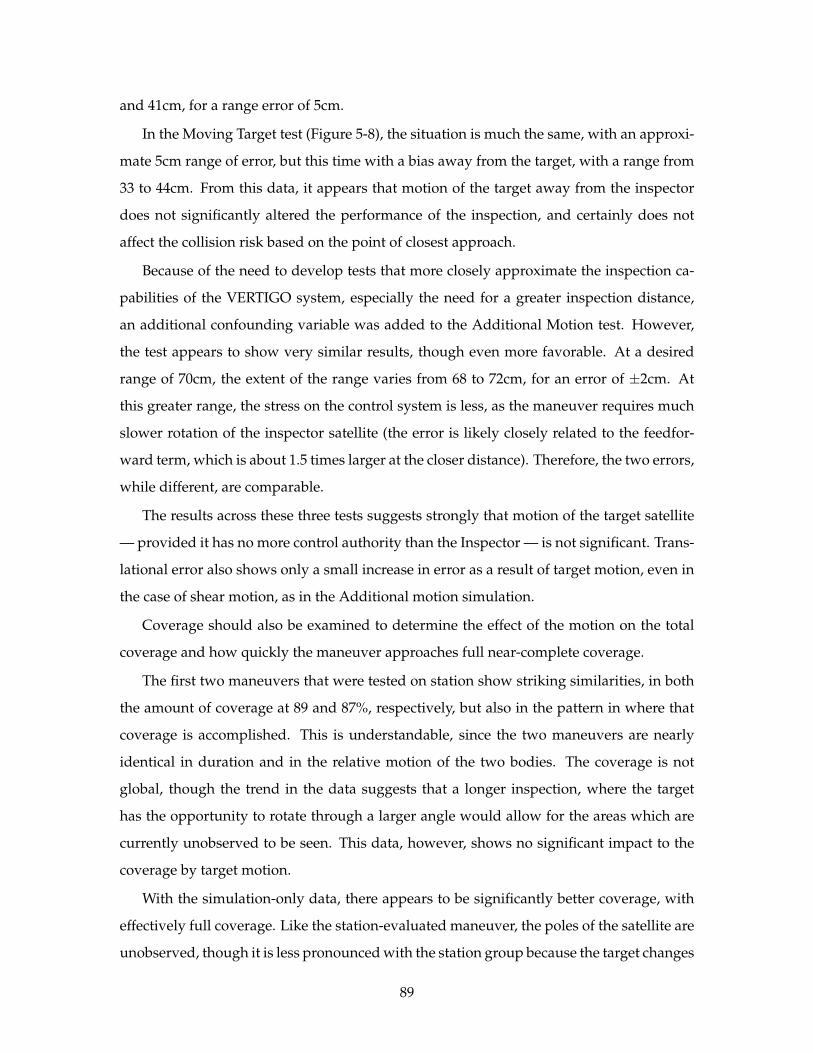
and 41cm, for a range error of 5cm.
In the Moving Target test (Figure 5-8), the situation is much the same, with an approxi-
mate 5cm range of error, but this time with a bias away from the target, with a range from
33 to 44cm. From this data, it appears that motion of the target away from the inspector
does not significantly altered the performance of the inspection, and certainly does not
affect the collision risk based on the point of closest approach.
Because of the need to develop tests that more closely approximate the inspection ca-
pabilities of the VERTIGO system, especially the need for a greater inspection distance,
an additional confounding variable was added to the Additional Motion test. However,
the test appears to show very similar results, though even more favorable. At a desired
range of 70cm, the extent of the range varies from 68 to 72cm, for an error of ±2cm. At
this greater range, the stress on the control system is less, as the maneuver requires much
slower rotation of the inspector satellite (the error is likely closely related to the feedfor-
ward term, which is about 1.5 times larger at the closer distance). Therefore, the two errors,
while different, are comparable.
The results across these three tests suggests strongly that motion of the target satellite
— provided it has no more control authority than the Inspector — is not significant. Trans-
lational error also shows only a small increase in error as a result of target motion, even in
the case of shear motion, as in the Additional motion simulation.
Coverage should also be examined to determine the effect of the motion on the total
coverage and how quickly the maneuver approaches full near-complete coverage.
The first two maneuvers that were tested on station show striking similarities, in both
the amount of coverage at 89 and 87%, respectively, but also in the pattern in where that
coverage is accomplished. This is understandable, since the two maneuvers are nearly
identical in duration and in the relative motion of the two bodies. The coverage is not
global, though the trend in the data suggests that a longer inspection, where the target
has the opportunity to rotate through a larger angle would allow for the areas which are
currently unobserved to be seen. This data, however, shows no significant impact to the
coverage by target motion.
With the simulation-only data, there appears to be significantly better coverage, with
effectively full coverage. Like the station-evaluated maneuver, the poles of the satellite are
unobserved, though it is less pronounced with the station group because the target changes
89
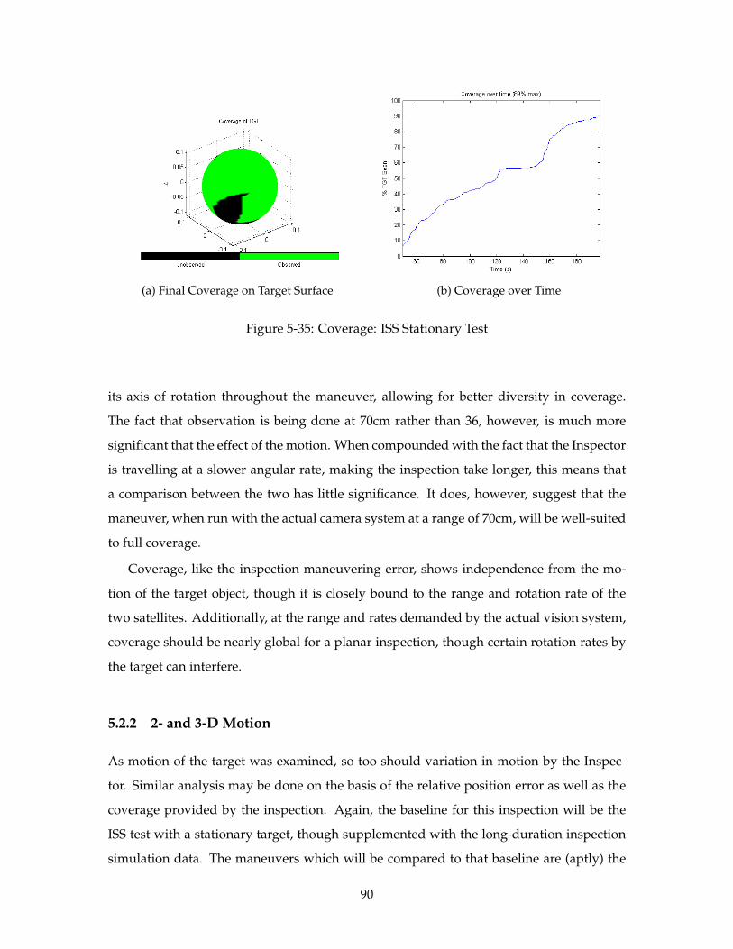
(a) Final Coverage on Target Surface (b) Coverage over Time
Figure 5-35: Coverage: ISS Stationary Test
its axis of rotation throughout the maneuver, allowing for better diversity in coverage.
The fact that observation is being done at 70cm rather than 36, however, is much more
significant that the effect of the motion. When compounded with the fact that the Inspector
is travelling at a slower angular rate, making the inspection take longer, this means that
a comparison between the two has little significance. It does, however, suggest that the
maneuver, when run with the actual camera system at a range of 70cm, will be well-suited
to full coverage.
Coverage, like the inspection maneuvering error, shows independence from the mo-
tion of the target object, though it is closely bound to the range and rotation rate of the
two satellites. Additionally, at the range and rates demanded by the actual vision system,
coverage should be nearly global for a planar inspection, though certain rotation rates by
the target can interfere.
5.2.2 2- and 3-D Motion
As motion of the target was examined, so too should variation in motion by the Inspec-
tor. Similar analysis may be done on the basis of the relative position error as well as the
coverage provided by the inspection. Again, the baseline for this inspection will be the
ISS test with a stationary target, though supplemented with the long-duration inspection
simulation data. The maneuvers which will be compared to that baseline are (aptly) the
90
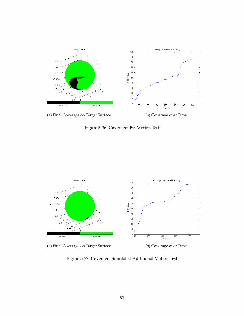
(a) Final Coverage on Target Surface (b) Coverage over Time
Figure 5-36: Coverage: ISS Motion Test
(a) Final Coverage on Target Surface (b) Coverage over Time
Figure 5-37: Coverage: Simulated Additional Motion Test
91
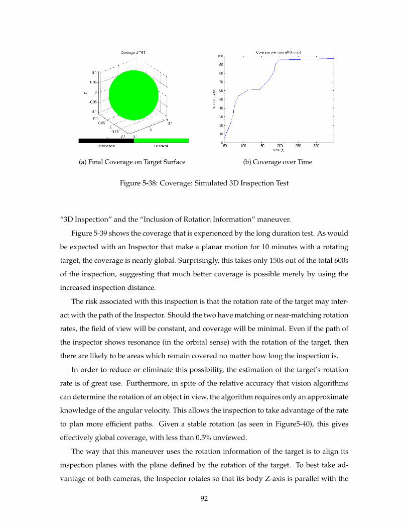
(a) Final Coverage on Target Surface (b) Coverage over Time
Figure 5-38: Coverage: Simulated 3D Inspection Test
“3D Inspection” and the “Inclusion of Rotation Information” maneuver.
Figure 5-39 shows the coverage that is experienced by the long duration test. As would
be expected with an Inspector that make a planar motion for 10 minutes with a rotating
target, the coverage is nearly global. Surprisingly, this takes only 150s out of the total 600s
of the inspection, suggesting that much better coverage is possible merely by using the
increased inspection distance.
The risk associated with this inspection is that the rotation rate of the target may inter-
act with the path of the Inspector. Should the two have matching or near-matching rotation
rates, the field of view will be constant, and coverage will be minimal. Even if the path of
the inspector shows resonance (in the orbital sense) with the rotation of the target, then
there are likely to be areas which remain covered no matter how long the inspection is.
In order to reduce or eliminate this possibility, the estimation of the target’s rotation
rate is of great use. Furthermore, in spite of the relative accuracy that vision algorithms
can determine the rotation of an object in view, the algorithm requires only an approximate
knowledge of the angular velocity. This allows the inspection to take advantage of the rate
to plan more efficient paths. Given a stable rotation (as seen in Figure5-40), this gives
effectively global coverage, with less than 0.5% unviewed.
The way that this maneuver uses the rotation information of the target is to align its
inspection planes with the plane defined by the rotation of the target. To best take ad-
vantage of both cameras, the Inspector rotates so that its body Z-axis is parallel with the
92
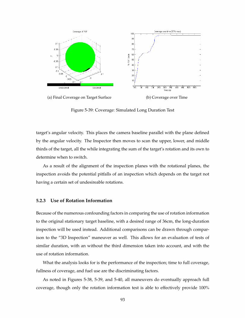
(a) Final Coverage on Target Surface (b) Coverage over Time
Figure 5-39: Coverage: Simulated Long Duration Test
target’s angular velocity. This places the camera baseline parallel with the plane defined
by the angular velocity. The Inspector then moves to scan the upper, lower, and middle
thirds of the target, all the while integrating the sum of the target’s rotation and its own to
determine when to switch.
As a result of the alignment of the inspection planes with the rotational planes, the
inspection avoids the potential pitfalls of an inspection which depends on the target not
having a certain set of undesireable rotations.
5.2.3 Use of Rotation Information
Because of the numerous confounding factors in comparing the use of rotation information
to the original stationary target baseline, with a desired range of 36cm, the long-duration
inspection will be used instead. Additional comparisons can be drawn through compar-
ison to the “3D Inspection” maneuver as well. This allows for an evaluation of tests of
similar duration, with an without the third dimension taken into account, and with the
use of rotation information.
What the analysis looks for is the performance of the inspection; time to full coverage,
fullness of coverage, and fuel use are the discriminating factors.
As noted in Figures 5-38, 5-39, and 5-40, all maneuvers do eventually approach full
coverage, though only the rotation information test is able to effectively provide 100%
93
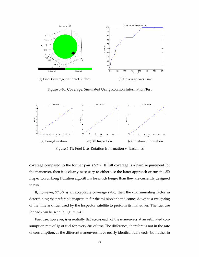
(a) Final Coverage on Target Surface (b) Coverage over Time
Figure 5-40: Coverage: Simulated Using Rotation Information Test
(a) Long-Duration (b) 3D Inspection (c) Rotation Information
Figure 5-41: Fuel Use: Rotation Information vs Baselines
coverage compared to the former pair’s 97%. If full coverage is a hard requirement for
the maneuver, then it is clearly necessary to either use the latter approach or run the 3D
Inspection or Long Duration algorithms for much longer than they are currently designed
to run.
If, however, 97.5% is an acceptable coverage ratio, then the discriminating factor in
determining the preferable inspection for the mission at hand comes down to a weighting
of the time and fuel used by the Inspector satellite to perform its maneuver. The fuel use
for each can be seen in Figure 5-41.
Fuel use, however, is essentially flat across each of the maneuvers at an estimated con-
sumption rate of 1g of fuel for every 30s of test. The difference, therefore is not in the rate
of consumption, as the different maneuvers have nearly identical fuel needs, but rather in
94
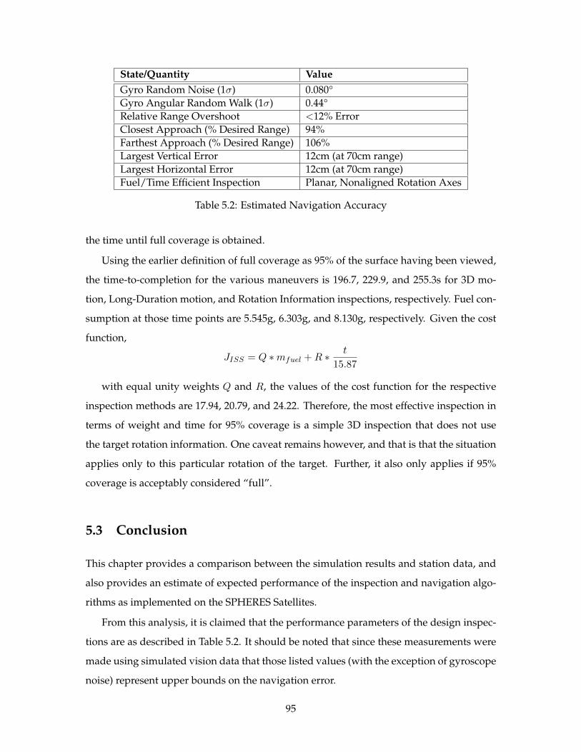
State/Quantity ValueGyro Random Noise (1σ) 0.080°Gyro Angular Random Walk (1σ) 0.44°Relative Range Overshoot <12% ErrorClosest Approach (% Desired Range) 94%Farthest Approach (% Desired Range) 106%Largest Vertical Error 12cm (at 70cm range)Largest Horizontal Error 12cm (at 70cm range)Fuel/Time Efficient Inspection Planar, Nonaligned Rotation Axes
Table 5.2: Estimated Navigation Accuracy
the time until full coverage is obtained.
Using the earlier definition of full coverage as 95% of the surface having been viewed,
the time-to-completion for the various maneuvers is 196.7, 229.9, and 255.3s for 3D mo-
tion, Long-Duration motion, and Rotation Information inspections, respectively. Fuel con-
sumption at those time points are 5.545g, 6.303g, and 8.130g, respectively. Given the cost
function,
JISS = Q ∗mfuel +R ∗ t
15.87
with equal unity weights Q and R, the values of the cost function for the respective
inspection methods are 17.94, 20.79, and 24.22. Therefore, the most effective inspection in
terms of weight and time for 95% coverage is a simple 3D inspection that does not use
the target rotation information. One caveat remains however, and that is that the situation
applies only to this particular rotation of the target. Further, it also only applies if 95%
coverage is acceptably considered “full”.
5.3 Conclusion
This chapter provides a comparison between the simulation results and station data, and
also provides an estimate of expected performance of the inspection and navigation algo-
rithms as implemented on the SPHERES Satellites.
From this analysis, it is claimed that the performance parameters of the design inspec-
tions are as described in Table 5.2. It should be noted that since these measurements were
made using simulated vision data that those listed values (with the exception of gyroscope
noise) represent upper bounds on the navigation error.
95
The consequences of the data is that inspections will be able to be conducted without
significant risk of collision. Further, the best estimate of the gyroscope random noise sug-
gests that 50Hz data has a deviation of 0.080°. Whether or not that meets performance re-
quirements for a vision system is dependent on the camera algorithms, but the low value
suggests that they will work for most situations. The low translational errors also bode
well for VERTIGO, since they suggest that it will be able to maintain pointing toward the
target object even if the target begins to move during the inspection. Further, since a 3-
minute inspection does not move out of plane by more than 10cm, when combined with
image processing tools, it will be possible to build an accurate 3D map — and achieve the
VERTIGO mission.
96

Chapter 6
Project Management of the VERTIGO
Payload
The story of the VERTIGO Program is one that will be familiar to many who are involved
in the development of spaceflight hardware. This chapter will delve into some of the chal-
lenges and successes that the program experienced and analyze the program from the
point of view of your author, the MIT Program Manager.
Throughout the chapter we will follow the program through two points of view: the
Product and the Process. We will examine how technical problems and approaches fed
back into the program management, and how the same management in all its forms in-
formed the final product in fabrication.
We will also show the initial timeline of the program and its evolution as it met the
realities of the engineering, scheduling, and other technical challenges. It will also cover
feedback on the program model — that of a fast-paced technical development program de-
signed to mature ground hardware up the technology readiness ladder. And finally it will
provide lessons learned for future student program managers, and military officers as a
part of the Space Engineering Academy program within MIT’s Space Systems Laboratory.
We begin with an exploration of the eight guiding principles which were used to guide
the development of the VERTIGO product and the leadership and engineering process
to develop that product. Figure 6-1 shows the two elements side by side, and how the
different legacies of the LIIVe and SPHERES Programs worked together with VERTIGO on
the way to delivery of flight hardware. This figure will guide the discussion throughout.
97
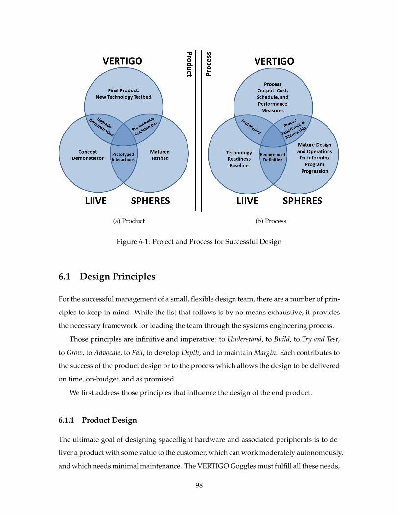
(a) Product (b) Process
Figure 6-1: Project and Process for Successful Design
6.1 Design Principles
For the successful management of a small, flexible design team, there are a number of prin-
ciples to keep in mind. While the list that follows is by no means exhaustive, it provides
the necessary framework for leading the team through the systems engineering process.
Those principles are infinitive and imperative: to Understand, to Build, to Try and Test,
to Grow, to Advocate, to Fail, to develop Depth, and to maintain Margin. Each contributes to
the success of the product design or to the process which allows the design to be delivered
on time, on-budget, and as promised.
We first address those principles that influence the design of the end product.
6.1.1 Product Design
The ultimate goal of designing spaceflight hardware and associated peripherals is to de-
liver a product with some value to the customer, which can work moderately autonomously,
and which needs minimal maintenance. The VERTIGO Goggles must fulfill all these needs,
98
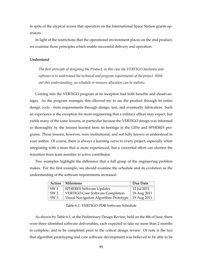
in spite of the atypical access that operation on the International Space Station grants op-
erators.
In light of the restrictions that the operational environment places on the end product,
we examine those principles which enable successful delivery and operation.
Understand
The first principle of designing the Product, in this case the VERTIGO hardware and
software is to understand the technical and program requirements of the project. With-
out this understanding, no schedule or resource allocation can be realistic.
Coming into the VERTIGO program at its inception had both benefits and disadvan-
tages. As the program manager, this allowed me to see the product through its entire
design cycle - from requirements through design, test, and eventually fabrication. Such
an experience is the exception for most engineering that a military officer may expect, but
yields many of the same lessons, in particular because the VERTIGO design was informed
so thoroughly by the lessons learned from its heritage in the LIIVe and SPHERES pro-
grams. Those lessons, however, were institutional, and not fully known or understood to
your author. Of course, there is always a learning curve to every project, especially when
integrating with a team that is more experienced, but a concerted effort can shorten the
transition from team member to active contributor.
Two examples highlight the difference that a full grasp of the engineering problem
makes. For the first example, we should examine the schedule and its evolution as the
understanding of the software requirements increased.
Action Milestone Due DateSW 1 SPHERES Software Updates 12 Jul 2011SW 2 VERTIGO Core Software Completion 19 Aug 2011SW 3 Visual Navigation Algorithm Prototype 19 Aug 2011
Table 6.1: VERTIGO PDR Software Schedule
As shown by Table 6.1, at the Preliminary Design Review, held on the 8th of June, there
were three identified software deliverables, each expected to take no more than 2 months
to complete, and to be completed prior to the critical design review. Of note is the fact
that algorithm prototyping and core software development was believed to be able to be
99
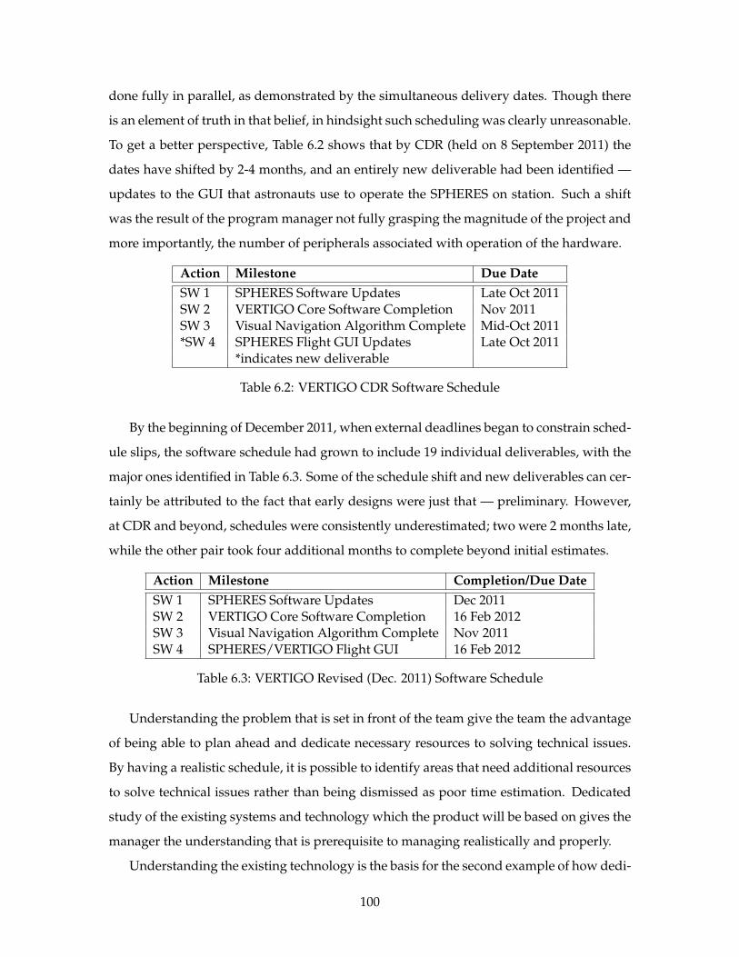
done fully in parallel, as demonstrated by the simultaneous delivery dates. Though there
is an element of truth in that belief, in hindsight such scheduling was clearly unreasonable.
To get a better perspective, Table 6.2 shows that by CDR (held on 8 September 2011) the
dates have shifted by 2-4 months, and an entirely new deliverable had been identified —
updates to the GUI that astronauts use to operate the SPHERES on station. Such a shift
was the result of the program manager not fully grasping the magnitude of the project and
more importantly, the number of peripherals associated with operation of the hardware.
Action Milestone Due DateSW 1 SPHERES Software Updates Late Oct 2011SW 2 VERTIGO Core Software Completion Nov 2011SW 3 Visual Navigation Algorithm Complete Mid-Oct 2011*SW 4 SPHERES Flight GUI Updates Late Oct 2011
*indicates new deliverable
Table 6.2: VERTIGO CDR Software Schedule
By the beginning of December 2011, when external deadlines began to constrain sched-
ule slips, the software schedule had grown to include 19 individual deliverables, with the
major ones identified in Table 6.3. Some of the schedule shift and new deliverables can cer-
tainly be attributed to the fact that early designs were just that — preliminary. However,
at CDR and beyond, schedules were consistently underestimated; two were 2 months late,
while the other pair took four additional months to complete beyond initial estimates.
Action Milestone Completion/Due DateSW 1 SPHERES Software Updates Dec 2011SW 2 VERTIGO Core Software Completion 16 Feb 2012SW 3 Visual Navigation Algorithm Complete Nov 2011SW 4 SPHERES/VERTIGO Flight GUI 16 Feb 2012
Table 6.3: VERTIGO Revised (Dec. 2011) Software Schedule
Understanding the problem that is set in front of the team give the team the advantage
of being able to plan ahead and dedicate necessary resources to solving technical issues.
By having a realistic schedule, it is possible to identify areas that need additional resources
to solve technical issues rather than being dismissed as poor time estimation. Dedicated
study of the existing systems and technology which the product will be based on gives the
manager the understanding that is prerequisite to managing realistically and properly.
Understanding the existing technology is the basis for the second example of how dedi-
100
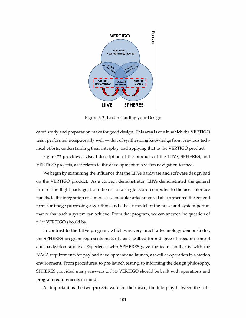
Figure 6-2: Understanding your Design
cated study and preparation make for good design. This area is one in which the VERTIGO
team performed exceptionally well — that of synthesizing knowledge from previous tech-
nical efforts, understanding their interplay, and applying that to the VERTIGO product.
Figure ?? provides a visual description of the products of the LIIVe, SPHERES, and
VERTIGO projects, as it relates to the development of a vision navigation testbed.
We begin by examining the influence that the LIIVe hardware and software design had
on the VERTIGO product. As a concept demonstrator, LIIVe demonstrated the general
form of the flight package, from the use of a single board computer, to the user interface
panels, to the integration of cameras as a modular attachment. It also presented the general
form for image processing algorithms and a basic model of the noise and system perfor-
mance that such a system can achieve. From that program, we can answer the question of
what VERTIGO should be.
In contrast to the LIIVe program, which was very much a technology demonstrator,
the SPHERES program represents maturity as a testbed for 6 degree-of-freedom control
and navigation studies. Experience with SPHERES gave the team familiarity with the
NASA requirements for payload development and launch, as well as operation in a station
environment. From procedures, to pre-launch testing, to informing the design philosophy,
SPHERES provided many answers to how VERTIGO should be built with operations and
program requirements in mind.
As important as the two projects were on their own, the interplay between the soft-
101
ware and hardware of each gave the VERTIGO team insights and understanding of how
the VERTIGO hardware should interact with SPHERES. Without the prototyped interac-
tions between the two sets of hardware, the serial communication protocol would have
been set back, as would modifications to the metrology system. Because those major el-
ements had been developed and tested out on SPHERES-LIIVe, SPHERES-VERTIGO was
able to learn what did and did not work, and even more importantly (for a short-duration
project), know what did not work. Having working hardware that could be built upon
and modified was the key enabling factor in the product being delivered within the short
15-month timeframe.
Those elements that were prototyped or otherwise studied on SPHERES-LIIVe that
informed the design of the SPHERES-VERTIGO product included:
1. Serial communication between the payload and the host SPHERE (later matured
with development of other payloads in addition to VERTIGO)
2. Mechanical fitting and interaction
3. Thermal management and component temperature limits
4. Component selection and shortcomings of certain parts, including reduced lifetime
at operating conditions
Had the system been started from scratch without being developed in a simple ground-
based system prior to launch, there would have been no way for the relatively small team
assigned to VERTIGO to complete its task in the time allotted. The benefit was that both
the team and its managers understood the lessons learned from the previously-developed
hardware.
Build
Build early and often. If you build it, you will understand it better, and the deadlines
associated with hardware build will motivate engineers to move from paper to product.
If you wait to build, you will have fewer chances to identify and fix those problems
which inevitably occur. Even worse, those that do crop up will be much more compli-
cated than those which appear early.
102
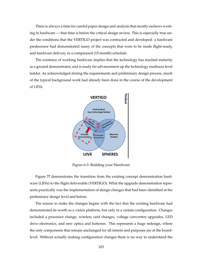
There is always a time for careful paper design and analysis that mostly eschews work-
ing in hardware — that time is before the critical design review. This is especially true un-
der the conditions that the VERTIGO project was contracted and developed: a hardware
predecessor had demonstrated many of the concepts that were to be made flight-ready,
and hardware delivery in a compressed (15-month) schedule.
The existence of working hardware implies that the technology has reached maturity
as a ground demonstrator, and is ready for advancement up the technology readiness level
ladder. As acknowledged during the requirements and preliminary design process, much
of the typical background work had already been done in the course of the development
of LIIVe.
Figure 6-3: Building your Hardware
Figure ?? demonstrates the transition from the existing concept demonstration hard-
ware (LIIVe) to the flight deliverable (VERTIGO). What the upgrade demonstration repre-
sents practically was the implementation of design changes that had been identified at the
preliminary design level and before.
The reason to make the changes begins with the fact that the existing hardware had
demonstrated its worth as a vision platform, but only in a certain configuration. Changes
included a processor change, wireless card changes, voltage converters upgrades, LED
drive electronics, and new optics and batteries. This represents a huge redesign, where
the only components that remain unchanged for all intents and purposes are at the board-
level. Without actually making configuration changes there is no way to understand the
103
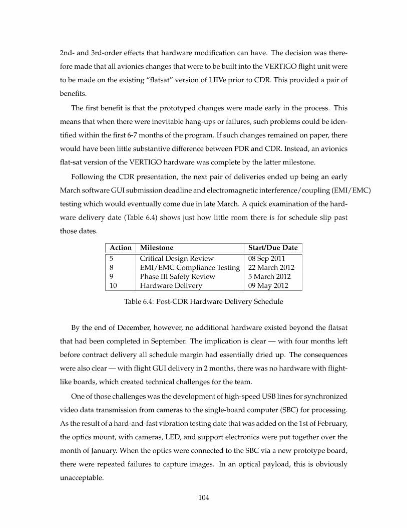
2nd- and 3rd-order effects that hardware modification can have. The decision was there-
fore made that all avionics changes that were to be built into the VERTIGO flight unit were
to be made on the existing “flatsat” version of LIIVe prior to CDR. This provided a pair of
benefits.
The first benefit is that the prototyped changes were made early in the process. This
means that when there were inevitable hang-ups or failures, such problems could be iden-
tified within the first 6-7 months of the program. If such changes remained on paper, there
would have been little substantive difference between PDR and CDR. Instead, an avionics
flat-sat version of the VERTIGO hardware was complete by the latter milestone.
Following the CDR presentation, the next pair of deliveries ended up being an early
March software GUI submission deadline and electromagnetic interference/coupling (EMI/EMC)
testing which would eventually come due in late March. A quick examination of the hard-
ware delivery date (Table 6.4) shows just how little room there is for schedule slip past
those dates.
Action Milestone Start/Due Date5 Critical Design Review 08 Sep 20118 EMI/EMC Compliance Testing 22 March 20129 Phase III Safety Review 5 March 201210 Hardware Delivery 09 May 2012
Table 6.4: Post-CDR Hardware Delivery Schedule
By the end of December, however, no additional hardware existed beyond the flatsat
that had been completed in September. The implication is clear — with four months left
before contract delivery all schedule margin had essentially dried up. The consequences
were also clear — with flight GUI delivery in 2 months, there was no hardware with flight-
like boards, which created technical challenges for the team.
One of those challenges was the development of high-speed USB lines for synchronized
video data transmission from cameras to the single-board computer (SBC) for processing.
As the result of a hard-and-fast vibration testing date that was added on the 1st of February,
the optics mount, with cameras, LED, and support electronics were put together over the
month of January. When the optics were connected to the SBC via a new prototype board,
there were repeated failures to capture images. In an optical payload, this is obviously
unacceptable.
104
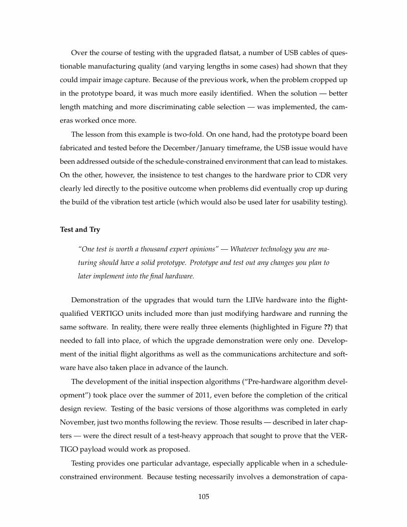
Over the course of testing with the upgraded flatsat, a number of USB cables of ques-
tionable manufacturing quality (and varying lengths in some cases) had shown that they
could impair image capture. Because of the previous work, when the problem cropped up
in the prototype board, it was much more easily identified. When the solution — better
length matching and more discriminating cable selection — was implemented, the cam-
eras worked once more.
The lesson from this example is two-fold. On one hand, had the prototype board been
fabricated and tested before the December/January timeframe, the USB issue would have
been addressed outside of the schedule-constrained environment that can lead to mistakes.
On the other, however, the insistence to test changes to the hardware prior to CDR very
clearly led directly to the positive outcome when problems did eventually crop up during
the build of the vibration test article (which would also be used later for usability testing).
Test and Try
“One test is worth a thousand expert opinions” — Whatever technology you are ma-
turing should have a solid prototype. Prototype and test out any changes you plan to
later implement into the final hardware.
Demonstration of the upgrades that would turn the LIIVe hardware into the flight-
qualified VERTIGO units included more than just modifying hardware and running the
same software. In reality, there were really three elements (highlighted in Figure ??) that
needed to fall into place, of which the upgrade demonstration were only one. Develop-
ment of the initial flight algorithms as well as the communications architecture and soft-
ware have also taken place in advance of the launch.
The development of the initial inspection algorithms (“Pre-hardware algorithm devel-
opment”) took place over the summer of 2011, even before the completion of the critical
design review. Testing of the basic versions of those algorithms was completed in early
November, just two months following the review. Those results — described in later chap-
ters — were the direct result of a test-heavy approach that sought to prove that the VER-
TIGO payload would work as proposed.
Testing provides one particular advantage, especially applicable when in a schedule-
constrained environment. Because testing necessarily involves a demonstration of capa-
105
Figure 6-4: Testing the Product
bility in place of a purely paper analysis, it shows confidence. Prior to the inspection
algorithm tests, the SPHERES gyros had not been used much for dead reckoning, and not
with the precision that vision-navigation prefers. The behavior and drift of those gyros
after years on orbit was not well-understood or studied. They had certainly not been used
for pose propagation from one camera frame to another, which requires fairly low noise.
By demonstrating the constraints on the random error and random walk, and physically
demonstrating the maneuver in a microgravity environment, confidence was built in the
SPHERES hardware to accomplish the missions prior to even launching the VERTIGO
payload.
Furthermore, that basic testing established a simple maneuvering algorithm which
could then be built upon without concerns that the basic premise was somehow flawed.
For future revisions, if the inspections do fail, then the problem is likely to be in the new
code, or in the hardware. Overall, by trying and testing the code on the original SPHERES
hardware, confidence was built. Expected performance was also established, and perfor-
mance was able to be baselined from it. Beyond the establishment of functional confidence
and a performance baseline, it also provided code that could be used to more accurately
test the hardware when it was completed.
During the course of the GUI testing from the original delivery date on 5 March until
an update delivery in early May, elements of the algorithm code were combined with code
which would handle communication between the SPHERES and VERTIGO. The develop-
106
ment of that code also followed the “Try it and Test it” approach to hardware, though that
was delivered with less lead time. Software was developed first with basic functional-
ity, and tested while adding additional functions. Its development followed the hardware
build. By usability testing, the software was functionally complete, but still somewhat
buggy, with some changes still needing to be implemented. By developing the GUI in
this piecemeal approach, it was possible to test while working to implement new pieces of
code, and allowed for the required feedback from the approval authorities reviewing the
software for NASA’s Payload Display Review Team (PDRT).
Grow
In everything you do, start with a known, be it working hardware/software or even a
full program, and then increase complexity.
All elements described in Figure 6-1a followed the motto to always grow — in sys-
tem knowledge and product capability. Though there is something to be said for parallel
development, a product developed for space cannot afford to have components designed
and developed in isolation for too long.
VERTIGO did this well, in part because the team was small, team members had rela-
tively well-defined areas of responsibility, and project forces demanded close cooperation.
The immediate project team, as it was first constituted post-CDR consisted of a pro-
gram manager, lead scientist, GUI programmer, two avionics (electrical) engineers, me-
chanical engineer, and two software developers, in the form of 7 people (the first two roles
were student-filled, the remainder, professional engineers). By having 7 people fill 6 dis-
tinct roles, there were few questions about where responsibilities lay for most tasks which
came down the pipeline. Later, when manufacturing began, another member was added
with responsibility for that task.
Forces within and external to the project also played a role. Once more, the compressed
timeline required quick, yet accurate decision-making. Schedule pressure forces changes
to be made through all elements. This forces team members to interact with one another al-
most daily. While the scope of the project makes this a burdensome requirement for larger
projects, and not for VERTIGO, the project could not keep to schedule without it. Almost
no time is lost to design changes trickling through the systems engineers because that re-
107
sponsibility on VERTIGO was held by all members. For instance, when manufacturing of
the prototype optics mount discovered difficulties routing cables and mounting boards,
solutions were found jointly between all team members, led by the mechanical engineer
and the assemblers.
Similarly, when modifications needed to be made to the electronics to fit within the
mechanical fixtures, the changes were made in a day by the two team members tasked
with that role, with the assemblers watching.
The program as a whole also followed the rule of growing from a known before mov-
ing to an unknown. LIIVe itself was a known quantity from which VERTIGO could evolve.
The inspection software began first as a simple circumnavigation maneuver, and then
added different paths to the inspection planner. Serial communication between the SPHERES
and the Goggles was first prototyped with the CSAC experiment and expanded upon with
simple message parsing and passing built into the SPHERES guest scientist code. After
that element was tested, it was combined with more advanced inspection algorithms that
were in turn tested on the ground and in simulation. Each element fell into place after
gradual steps.
This approach has two significant advantages over others. If subsystem interaction is
largely on paper, once the designs are implemented, they must be integrated. After fully
designing a subsystem, designs are not partiularly malleable. Furthermore, since most
problems arise at interfaces, most time is then spent to combine subsystems. By constantly
integrating, improving, and reintegrating, the design process is more responsive and fast.
The downside to this approach is that it depends on the ability of a design to be able
to evolve from one state to another. Such an approach must either accept the possibility of
non-optimality in design (as the design evolves, the need to always be operable constrains
the nature of changes of design) or be willing to keep some elements from integrating until
project completion.
On the balance, however, the approach is beneficial in maintaining a rapid design-
to-flight schedule, while minimizing the chance for significant miscommunication which
hamstrings the project until a full redesign can be accomplished. In this manner, the
lessons are applicable even to larger projects, particularly at the subsystem level where
different components much some together.
The design and evolution of the VERTIGO product, however, is not the only reason
108
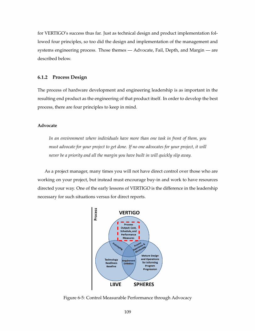
for VERTIGO’s success thus far. Just as technical design and product implementation fol-
lowed four principles, so too did the design and implementation of the management and
systems engineering process. Those themes — Advocate, Fail, Depth, and Margin — are
described below.
6.1.2 Process Design
The process of hardware development and engineering leadership is as important in the
resulting end product as the engineering of that product itself. In order to develop the best
process, there are four principles to keep in mind.
Advocate
In an environment where individuals have more than one task in front of them, you
must advocate for your project to get done. If no one advocates for your project, it will
never be a priority and all the margin you have built in will quickly slip away.
As a project manager, many times you will not have direct control over those who are
working on your project, but instead must encourage buy-in and work to have resources
directed your way. One of the early lessons of VERTIGO is the difference in the leadership
necessary for such situations versus for direct reports.
Figure 6-5: Control Measurable Performance through Advocacy
109
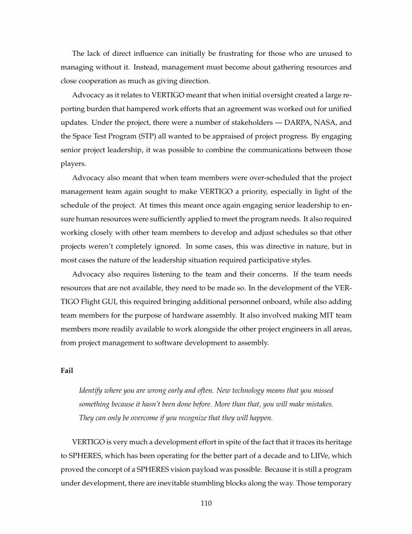
The lack of direct influence can initially be frustrating for those who are unused to
managing without it. Instead, management must become about gathering resources and
close cooperation as much as giving direction.
Advocacy as it relates to VERTIGO meant that when initial oversight created a large re-
porting burden that hampered work efforts that an agreement was worked out for unified
updates. Under the project, there were a number of stakeholders — DARPA, NASA, and
the Space Test Program (STP) all wanted to be appraised of project progress. By engaging
senior project leadership, it was possible to combine the communications between those
players.
Advocacy also meant that when team members were over-scheduled that the project
management team again sought to make VERTIGO a priority, especially in light of the
schedule of the project. At times this meant once again engaging senior leadership to en-
sure human resources were sufficiently applied to meet the program needs. It also required
working closely with other team members to develop and adjust schedules so that other
projects weren’t completely ignored. In some cases, this was directive in nature, but in
most cases the nature of the leadership situation required participative styles.
Advocacy also requires listening to the team and their concerns. If the team needs
resources that are not available, they need to be made so. In the development of the VER-
TIGO Flight GUI, this required bringing additional personnel onboard, while also adding
team members for the purpose of hardware assembly. It also involved making MIT team
members more readily available to work alongside the other project engineers in all areas,
from project management to software development to assembly.
Fail
Identify where you are wrong early and often. New technology means that you missed
something because it hasn’t been done before. More than that, you will make mistakes.
They can only be overcome if you recognize that they will happen.
VERTIGO is very much a development effort in spite of the fact that it traces its heritage
to SPHERES, which has been operating for the better part of a decade and to LIIVe, which
proved the concept of a SPHERES vision payload was possible. Because it is still a program
under development, there are inevitable stumbling blocks along the way. Those temporary
110
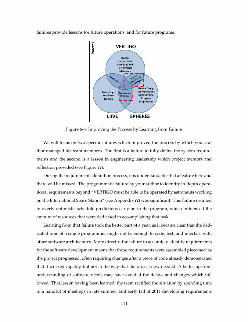
failures provide lessons for future operations, and for future programs.
Figure 6-6: Improving the Process by Learning from Failure
We will focus on two specific failures which improved the process by which your au-
thor managed his team members. The first is a failure to fully define the system require-
ments and the second is a lesson in engineering leadership which project mentors and
reflection provided (see Figure ??).
During the requirements definition process, it is understandable that a feature here and
there will be missed. The programmatic failure by your author to identify in-depth opera-
tional requirements beyond “VERTIGO must be able to be operated by astronauts working
on the International Space Station” (see Appendix ??) was significant. This failure resulted
in overly optimistic schedule predictions early on in the program, which influenced the
amount of resources that were dedicated to accomplishing that task.
Learning from that failure took the better part of a year, as it became clear that the ded-
icated time of a single programmer might not be enough to code, test, and interface with
other software architectures. More directly, the failure to accurately identify requirements
for the software development means that those requirements were assembled piecemeal as
the project progressed, often requiring changes after a piece of code already demonstrated
that it worked capably, but not in the way that the project now needed. A better up-front
understanding of software needs may have avoided the delays and changes which fol-
lowed. That lesson having been learned, the team rectified the situation by spending time
in a handful of meetings in late summer and early fall of 2011 developing requirements
111
and design choices so that the GUI development could proceed with more direction.
The second failure of project management was really a failure of leadership at the
project manager level. By December of 2011, with the first major delivery about two and
a half months away, there was no hardware available to test software on. This was the re-
sult of a leadership strategy which was more generally suited for a situation more closely
tied to those for which your author had more experience: those with military chains of
command in which the task at hand was well-defined and which all members had directly
applicable previous experience (it was not an engineering project, each of which has its
own nuance) and few other duties. Such an approach was not suited to the open-ended
engineering challenge posed by VERTIGO, where team members had other responsibilities
and where resources could only be mustered in an indirect way. That difference meant that
a hands-off approach was not the best option, and instead closer teamwork was needed.
This failure was overcome through mentoring and guidance provided by those MIT
managers who had been through the engineering leadership challenge previously with
SPHERES. The solution was multifaceted.
First, additional resources were sourced (indirectly) so that software development had
additional resources to meet their deadline. The additional manpower allowed VERTIGO
to meet its software deadlines. Additional team members were brought on board with
expertise in assembly to speed up the build process.
Second, the project management team began to advocate more strongly for those re-
sources which were already assigned to the team. Previously, other projects had been given
priority over VERTIGO, which meant that the total man-hours spent were not enough to
match what was needed. By working with over-scheduled team members to prioritize
project-related work in light of fast-approaching deadlines. Perhaps most importantly, the
MIT team began to work heavily in the industry partner’s own facilities, providing faster
feedback and interaction. By speeding up the communication loop by orders of magni-
tude, as well as bringing MIT resources directly to bear, work was able to quickly pick up.
Waiting times shortened. Without the closer interaction and resultant improved commu-
nication, there was little chance that the early delivery deadlines would have been met.
The final factor which was able to influence the course of the project was the addition
of a vibration testing deadline a month in advance of the software delivery. Though it
increased schedule pressure considerably, the hard-and-fast date associate with it pushed
112
the team to develop working optics and support avionics. The hard deadline compelled
the manufacturing of boards and mechanical fixtures, rather than remaining in assembly
and CAD layouts. By manufacturing (see Subsection 6.1.1), the team was able to identify
problems in the design. Perhaps just as importantly, by having working hardware ready
in advance of the software deadline, that software was able to be tested on flight-like hard-
ware rather than only on simulators alone.
As these two examples show, failures need not doom a project. Instead, take the lessons
from those failures, adapt, and use them to improve the process by which the program is
managed.
Depth
Your development team will have some area in which there is no “reserve” to call upon.
Find that shortage and fix it.
For the process by which you build hardware and software to be successful, you must
create depth in your team. Different approaches are possible, but all require an investment
of financial or human resources.
Though it is by no means exclusive to the software development side of VERTIGO,
the team had a single member working on the payload-specific GUI from conception un-
til about two months before initial delivery. Combined with an underestimation of the
software tasks early in the design process, as well as software modifications which were
implemented later than desirable, this pushed the software delivery date from its original
October 2011 date (Table 6.2) to February 2012 (Table 6.3), to an eventual initial delivery in
March 2012 with a final delivery in early May 2012.
The team members were more than competent at their tasks, but it was up to program
management to provide the necessary resources for those members to achieve the sched-
ule. Quite literally, there were just not enough hours in the day for a single person to
accomplish the tasks that were being asked of them. At that point, it is incumbent upon
the program manager to provide those additional resources in concert with those who
control the financial and personnel resources. This is a shift in the “Iron Triangle” of Cost,
Schedule, and Performance, but one which must be made when one of those elements has
fallen out of balance, as discussed in Section 6.2 of this chapter.
113
Furthermore, those resources must be applied in a manner and with such timing that
they neither detract from the current efforts nor require so much extra up-front investment
that the benefits of additional team members is null. In the case of VERTIGO, this was
achieved by bringing in the programmer of the original SPHERES GUI (from the 2006
launch delivery) about two-and-a-half months prior to Flight GUI initial delivery to help
with integration and coding support. Doing so allowed both of these conditions to be met
— the training burden was minimal, and the resource was applied with just enough time
to make a difference before the only time remaining had to be devoted to testing.
Adding depth to the team in places where it needs it most also provides an added
benefit: returning margin to the schedule. When unexpected issues appear, from illness
to additional projects, a team which has depth can absorb the impact of the lost team
member much better. During the EMI unit build, the loss of one member to illness would
have been catastrophic save for the fact that when it occurred, the team was able to very
quickly adjust because each member was familiar with most other project elements. As a
result, the team did move slower, but was still able to manufacture and test boards and
integrate the units before shipping them out for testing.
Such an experience also implies that developing depth does not necessarily mean an
influx fo resources beyond those that are already available. On the VERTIGO team, though
each segment of the project (Mechanical, Electrical, Software, Algorithms, etc) are nomi-
nally separate entities, with separate team members, as noted in Subsection 6.1.1 (“Grow”),
the team knew well the tasks and concerns of others. This meant that some depth was built
into the team, though responsibilities were very specifically divided. In many instances,
though the mechanical engineer is responsible for assembly/disassembly of the package,
during protoflight (EMI/EMC unit) assembly, both your author as program manager and
one of the electrical engineers would fill that role. Likewise, during assembly of the optics
mount, which behaves temperamentally, requiring fine alignment of a number of different
parts, there were three or four team members on a team of eight who became competent
in performing the job. As a caveat, this does not imply that team members are not indis-
pensable in their own roles, but only that as engineers it is often possible for a group that
works very closely with each other to supplement each other. With this approach, the re-
sponsibilities do not disappear, but the tasks can be filled by a team that is flexible, with
sufficient knowledge and preparation by other team members.
114
Depth, therefore is achievable in at least two ways: by assigning additional resources,
be they financial or human, to achieve a task, or by developing team members to be able to
complement one another and support each other when internal and external demands re-
quire it. The first is the preferable when significant resources are required which demands
very specialized skills or experience, while the second approach is acceptable when in a
constrained environment that demands project-specific experience and engineering skills.
Margin
If you’re a hardware engineer, your software estimates are off by at least 100%; Not
only in how long development will take, but in how much software is needed. Recognize
what you don’t know and add margin for that.
Then add some more.
One of the most difficult elements in managing the process by which a project is com-
pleted is estimating the time that it will take for each part to be completed. Managing
margin and schedule is what enables the rest of the process elements to fall into place.
Without a good handle, it is much more difficult to muster the proper depth and advocacy
for the project.
An understanding of the project (see subsection 6.1.1) is what contributes most to suc-
cessfully managing this process element. Figure ?? shows those elements which played a
significant role is growing, shrinking, and generally informing schedule margins over the
course of the VERTIGO project.
As has clearly been demonstrated previously (Tables 6.1, 6.2, and 6.3), accurately schedul-
ing software was your author’s most difficult part of maintaining schedule. That estima-
tion ability increased as the process itself became more concrete. Two elements played a
role in that: prototyping of the changes required, and learning lessons from the SPHERES
experience.
To address the former, we start with the LIIVe program, with all of its working electron-
ics and software. The results of that program were not flight-ready, but did demonstrate
a technology readiness near TRL 5. By making modifications to that hardware and proto-
typing the new boards, the effects of those changes became more pronounced. For the sake
of identifying particulars, let us focus on the changes necessary in developing the optics to
115
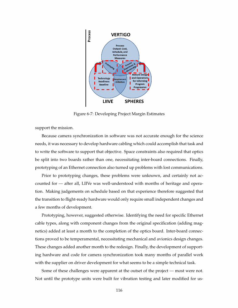
Figure 6-7: Developing Project Margin Estimates
support the mission.
Because camera synchronization in software was not accurate enough for the science
needs, it was necessary to develop hardware cabling which could accomplish that task and
to write the software to support that objective. Space constraints also required that optics
be split into two boards rather than one, necessitating inter-board connections. Finally,
prototyping of an Ethernet connection also turned up problems with lost communications.
Prior to prototyping changes, these problems were unknown, and certainly not ac-
counted for — after all, LIIVe was well-understood with months of heritage and opera-
tion. Making judgements on schedule based on that experience therefore suggested that
the transition to flight-ready hardware would only require small independent changes and
a few months of development.
Prototyping, however, suggested otherwise. Identifying the need for specific Ethernet
cable types, along with component changes from the original specification (adding mag-
netics) added at least a month to the completion of the optics board. Inter-board connec-
tions proved to be temperamental, necessitating mechanical and avionics design changes.
These changes added another month to the redesign. Finally, the development of support-
ing hardware and code for camera synchronization took many months of parallel work
with the supplier on driver development for what seems to be a simple technical task.
Some of these challenges were apparent at the outset of the project — most were not.
Not until the prototype units were built for vibration testing and later modified for us-
116
ability testing were many of these issues identified and resolved. Early expectations were
that hardware would be complete months ahead of the contract delivery date. Experi-
ence showed that such estimation was optimistic. From this, there are two approaches to
dealing with this uncertainty:
1. Build the schedule to a “horizon”. The best information you have at any given time
gets less accurate the further into the future you try to predict. To counteract the
growth in uncertainty, predict only to the point you can make reasonably accurate
judgements. That may be to the next deliverable or only to the next two months. This
allows for more accurate predictions, but completely ignores long-term planning.
2. Develop increasingly large margins over time, and decrease them not based on the
maturity of the design, but an estimate of the uncertainty that you have in the project.
While this aids in long-term planning, it may unfortunately give a false sense of
security, as a lack of knowledge about potential challenges with a technical problem
can cause an underestimation of the schedule risk.
Combining the two, by predicting accurate dates in the short-term, and putting margin
for both expected design issues and unexpected challenges on longer-term deliverables
will provide the best estimation of future schedule performance.
We now move to discuss the latter element, that of the applying the lessons learned
from the development and operation of the SPHERES satellites. As opposed to informing
the process for developing hardware, those lessons instead provide an understanding of
the operations development process.
Most satellites are in some way operated using human input rather than fully au-
tonomously. SPHERES-VERTIGO is no exception, and indeed, as a testbed operated on
the ground by students and on the ISS by astronauts, there are set procedures used to con-
trol those interactions. From SPHERES, the MIT team has learned a number of lessons, a
few of which follow:
1. Simplify interfaces — Astronauts are necessarily time constrained when they learn
to operate their payloads, and with training often happening months in advance of
a launch, it is likely that much of the training may be forgotten. From SPHERES,
the lesson was clear: keep design simple and clear and as a default present only the
information that is needed for nominal operations. From the beginning of GUI and
117
hardware design, this concept was kept in mind. The VERTIGO GUI presents no
additional options to the SPHERES GUI aside from the capability to load a file, per-
form a shutdown, download data, and if desired to switch the camera view seen.
Only three switches are immediately visible on the hardware: Power, reset, and LED
enable. By keeping the design simple, it simplifies the procedures, and streamlines
test sessions, as additional complexity in science and design does not transfer signif-
icant complexity in interfaces to the astronaut operators.
2. Provide debugging tools — Nearly everyone in the chain from those who provide
funding to astronauts who operate the payload to those who review paperwork sub-
missions want to see the mission succeed. By providing those tools in an easily ac-
cessible format, when things inevitably go wrong, much more data will be available
much faster, with much more accuracy and detail. Just as various debug tools within
the SPHERES software allows for large amounts of data collection and transmis-
sion, the use of which inspired and informed VERTIGO’s design. The flight GUI
was given a dedicated “maintenance mode” in order to run maintenance scripts and
change settings, while providing feedback to astronauts and ground scientists as to
the state of the Goggles. The development of these tools aid in on-orbit operations
as well as ground testing, providing easy access to the most relevant information
for developers. Additional debug options were also built into the design from the
beginning.
3. Hard-code nothing — While nothing may be a slight exaggeration, the ability to mod-
ify parameters for a GUI or test code is easier both procedurally, as it avoids multiple
code compilations, as well as programmatically, as far less paperwork is required for
software change approval.
Each of these lessons was taken into account in developing the procedures and design
for the system. As a result, when the first prototypes were in production (and especially
after the protoflight units were built), debugging was far simpler than it otherwise might
have been. Extracting performance data allowed the development team to identify faults
as varied as communication errors, camera synchronization errors, and much without hav-
ing to disassemble the entire system for every problem. More directly, by designing sim-
plicity and flexibility into the design from the beginning, NASA approval was far easier to
118
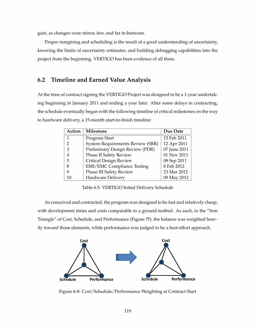
gain, as changes were minor, few, and far in-between.
Proper margining and scheduling is the result of a good understanding of uncertainty,
knowing the limits of uncertainty estimates, and building debugging capabilities into the
project from the beginning. VERTIGO has been evidence of all three.
6.2 Timeline and Earned Value Analysis
At the time of contract signing the VERTIGO Project was designed to be a 1-year undertak-
ing beginning in January 2011 and ending a year later. After some delays in contracting,
the schedule eventually began with the following timeline of critical milestones on the way
to hardware delivery, a 15-month start-to-finish timeline:
Action Milestone Due Date1 Program Start 15 Feb 20112 System Requirements Review (SRR) 12 Apr 20113 Preliminary Design Review (PDR) 07 June 20114 Phase II Safety Review 01 Nov 20115 Critical Design Review 08 Sep 20118 EMI/EMC Compliance Testing 8 Feb 20129 Phase III Safety Review 23 Mar 201210 Hardware Delivery 09 May 2012
Table 6.5: VERTIGO Initial Delivery Schedule
As conceived and contracted, the program was designed to be fast and relatively cheap,
with development times and costs comparable to a ground testbed. As such, in the “Iron
Triangle” of Cost, Schedule, and Performance (Figure ??), the balance was weighted heav-
ily toward those elements, while performance was judged to be a best-effort approach.
Figure 6-8: Cost/Schedule/Performance Weighting at Contract Start
119
6.2.1 Initial Design Period
Such a schedule was aggressive, especially with a small (yet motivated and competent)
team. Indeed, in many areas the development team was a single individual — one me-
chanical engineer, one electrical engineer, one vision researcher, one software developer
— though some relief was granted, by bringing engineers who had worked on the project
in the past to create depth in the software and avionics areas, and bringing outside re-
searchers to work on the vision algorithms and libraries which would inform the software
design.
Also critical to note is that the schedule gives just shy of 15 months from Program Start
to Hardware Delivery, with 2 months of development time given to SRR and PDR, and
3 months for preparation for CDR. The 7 months of preparation for flight hardware had
positives and negatives attached to them. On the positive side, that meant that changes
to the already existing precursor hardware (from LIIVe) were able to be experimentally
checked out, with technical issues being sorted out before they were implemented into in
the flight hardware development path. By dedicating 7 months to developing changes to
hardware which would not fly, significant time was spent which may have been better
spent on more flight-like hardware. On the balance, the dedicated development time was
advantageous to the team because it allowed two things to happen:
1. Changes could be compared and baselined to a working vision system.
2. Technical issues could be better isolated before they became intertwined on an untested
flight system.
Additionally, it allowed most changes to be identified prior to the CDR presentation.
The Systems Requirements Review, 2 months after nominal program start was a review
of the requirements that had been developed at the System, Functional, and Subsystem
levels. Those requirements demonstrated a lack of software experience in flight programs
of your author, as well as an understanding of the software needs that is typical of many
spaceflight programs. In the entire requirements document, out of 40 subsystem level
requirements, software requirements were directly addressed in only 4-5 — 10% of the
requirements. At the Functional level, the number was only slightly better at 5/30, barely
17%.
120
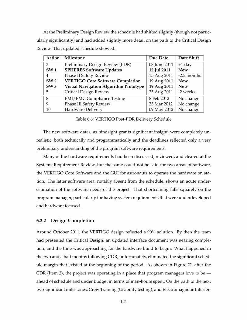
At the Preliminary Design Review the schedule had shifted slightly (though not partic-
ularly significantly) and had added slightly more detail on the path to the Critical Design
Review. That updated schedule showed:
Action Milestone Due Date Date Shift3 Preliminary Design Review (PDR) 08 June 2011 +1 daySW 1 SPHERES Software Updates 12 Jul 2011 New4 Phase II Safety Review 15 Aug 2011 -2.5 monthsSW 2 VERTIGO Core Software Completion 19 Aug 2011 NewSW 3 Visual Navigation Algorithm Prototype 19 Aug 2011 New5 Critical Design Review 25 Aug 2011 -2 weeks8 EMI/EMC Compliance Testing 8 Feb 2012 No change9 Phase III Safety Review 23 Mar 2012 No change10 Hardware Delivery 09 May 2012 No change
Table 6.6: VERTIGO Post-PDR Delivery Schedule
The new software dates, as hindsight grants significant insight, were completely un-
realistic, both technically and programmatically and the deadlines reflected only a very
preliminary understanding of the program software requirements.
Many of the hardware requirements had been discussed, reviewed, and cleared at the
Systems Requirement Review, but the same could not be said for two areas of software,
the VERTIGO Core Software and the GUI for astronauts to operate the hardware on sta-
tion. The latter software area, notably absent from the schedule, shows an acute under-
estimation of the software needs of the project. That shortcoming falls squarely on the
program manager, particularly for having system requirements that were underdeveloped
and hardware focused.
6.2.2 Design Completion
Around October 2011, the VERTIGO design reflected a 90% solution. By then the team
had presented the Critical Design, an updated interface document was nearing comple-
tion, and the time was approaching for the hardware build to begin. What happened in
the two and a half months following CDR, unfortunately, eliminated the significant sched-
ule margin that existed at the beginning of the period. As shown in Figure ??, after the
CDR (Item 2), the project was operating in a place that program managers love to be —
ahead of schedule and under budget in terms of man-hours spent. On the path to the next
two significant milestones, Crew Training (Usability testing), and Electromagnetic Interfer-
121
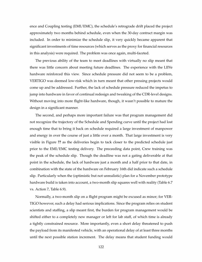
ence and Coupling testing (EMI/EMC), the schedule’s retrograde drift placed the project
approximately two months behind schedule, even when the 30-day contract margin was
included. In order to minimize the schedule slip, it very quickly became apparent that
significant investments of time resources (which serves as the proxy for financial resources
in this analysis) were required. The problem was once again, multi-faceted.
The previous ability of the team to meet deadlines with virtually no slip meant that
there was little concern about meeting future deadlines. The experience with the LIIVe
hardware reinforced this view. Since schedule pressure did not seem to be a problem,
VERTIGO was deemed low-risk which in turn meant that other pressing projects would
come up and be addressed. Further, the lack of schedule pressure reduced the impetus to
jump into hardware in favor of continual redesign and tweaking of the CDR-level designs.
Without moving into more flight-like hardware, though, it wasn’t possible to mature the
design in a significant manner.
The second, and perhaps more important failure was that program management did
not recognize the trajectory of the Schedule and Spending curve until the project had lost
enough time that to bring it back on schedule required a large investment of manpower
and energy in over the course of just a little over a month. That large investment is very
visible in Figure ?? as the deliveries begin to tack closer to the predicted schedule just
prior to the EMI/EMC testing delivery. The preceeding data point, Crew training was
the peak of the schedule slip. Though the deadline was not a gating deliverable at that
point in the schedule, the lack of hardware just a month and a half prior to that date, in
combination with the state of the hardware on February 16th did indicate such a schedule
slip. Particularly when the (optimistic but not unrealistic) plan for a November prototype
hardware build is taken into account, a two-month slip squares well with reality (Table 6.7
vs. Action 7, Table 6.9).
Normally, a two-month slip on a flight program might be excused as minor; for VER-
TIGO however, such a delay had serious implications. Since the program relies on student
scientists and staffing, a slip meant first, the burden for program management would be
shifted either to a completely new manager or left for lab staff, of which time is already
a tightly constrained resource. More importantly, even a short delay threatened to push
the payload from its manifested vehicle, with an operational delay of at least three months
until the next possible station increment. The delay means that student funding would
122
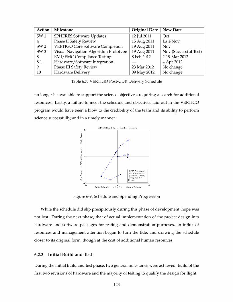
Action Milestone Original Date New DateSW 1 SPHERES Software Updates 12 Jul 2011 Oct4 Phase II Safety Review 15 Aug 2011 Late NovSW 2 VERTIGO Core Software Completion 19 Aug 2011 NovSW 3 Visual Navigation Algorithm Prototype 19 Aug 2011 Nov (Successful Test)8 EMI/EMC Compliance Testing 8 Feb 2012 2-19 Mar 20128.1 Hardware/Software Integration — 4 Apr 20129 Phase III Safety Review 23 Mar 2012 No change10 Hardware Delivery 09 May 2012 No change
Table 6.7: VERTIGO Post-CDR Delivery Schedule
no longer be available to support the science objectives, requiring a search for additional
resources. Lastly, a failure to meet the schedule and objectives laid out in the VERTIGO
program would have been a blow to the credibility of the team and its ability to perform
science successfully, and in a timely manner.
Figure 6-9: Schedule and Spending Progression
While the schedule did slip precipitously during this phase of development, hope was
not lost. During the next phase, that of actual implementation of the project design into
hardware and software packages for testing and demonstration purposes, an influx of
resources and management attention began to turn the tide, and drawing the schedule
closer to its original form, though at the cost of additional human resources.
6.2.3 Initial Build and Test
During the initial build and test phase, two general milestones were achieved: build of the
first two revisions of hardware and the majority of testing to qualify the design for flight.
123
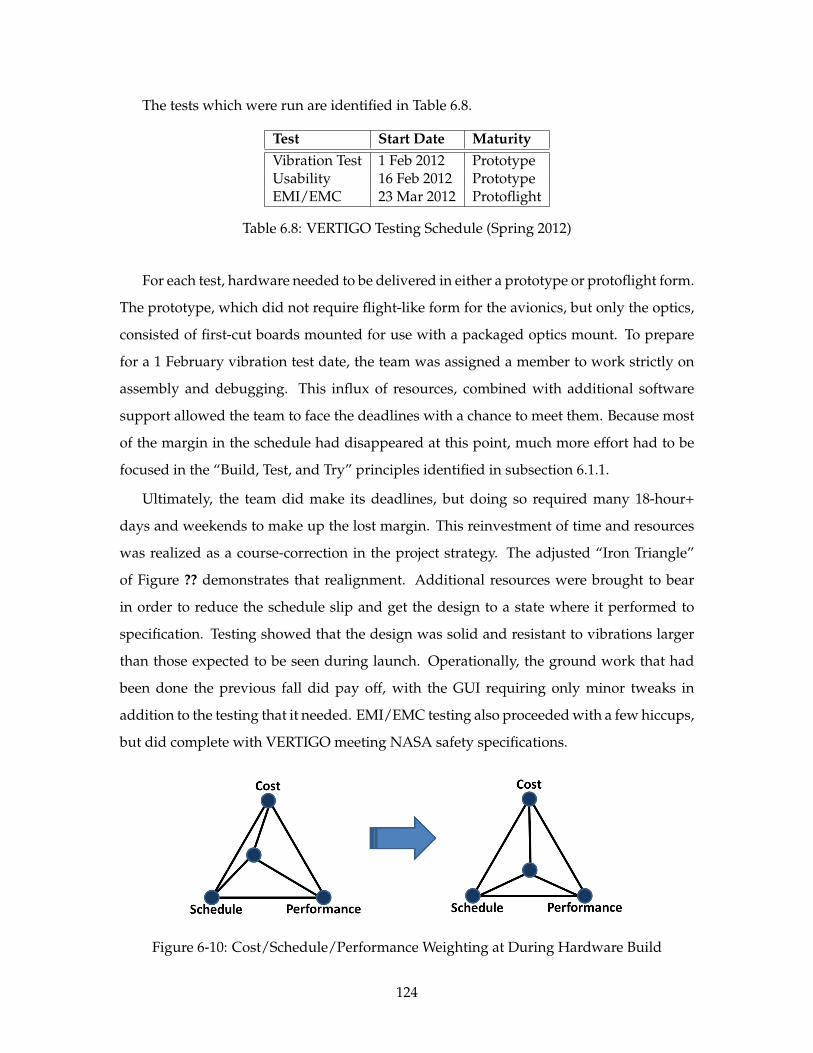
The tests which were run are identified in Table 6.8.
Test Start Date MaturityVibration Test 1 Feb 2012 PrototypeUsability 16 Feb 2012 PrototypeEMI/EMC 23 Mar 2012 Protoflight
Table 6.8: VERTIGO Testing Schedule (Spring 2012)
For each test, hardware needed to be delivered in either a prototype or protoflight form.
The prototype, which did not require flight-like form for the avionics, but only the optics,
consisted of first-cut boards mounted for use with a packaged optics mount. To prepare
for a 1 February vibration test date, the team was assigned a member to work strictly on
assembly and debugging. This influx of resources, combined with additional software
support allowed the team to face the deadlines with a chance to meet them. Because most
of the margin in the schedule had disappeared at this point, much more effort had to be
focused in the “Build, Test, and Try” principles identified in subsection 6.1.1.
Ultimately, the team did make its deadlines, but doing so required many 18-hour+
days and weekends to make up the lost margin. This reinvestment of time and resources
was realized as a course-correction in the project strategy. The adjusted “Iron Triangle”
of Figure ?? demonstrates that realignment. Additional resources were brought to bear
in order to reduce the schedule slip and get the design to a state where it performed to
specification. Testing showed that the design was solid and resistant to vibrations larger
than those expected to be seen during launch. Operationally, the ground work that had
been done the previous fall did pay off, with the GUI requiring only minor tweaks in
addition to the testing that it needed. EMI/EMC testing also proceeded with a few hiccups,
but did complete with VERTIGO meeting NASA safety specifications.
Figure 6-10: Cost/Schedule/Performance Weighting at During Hardware Build
124
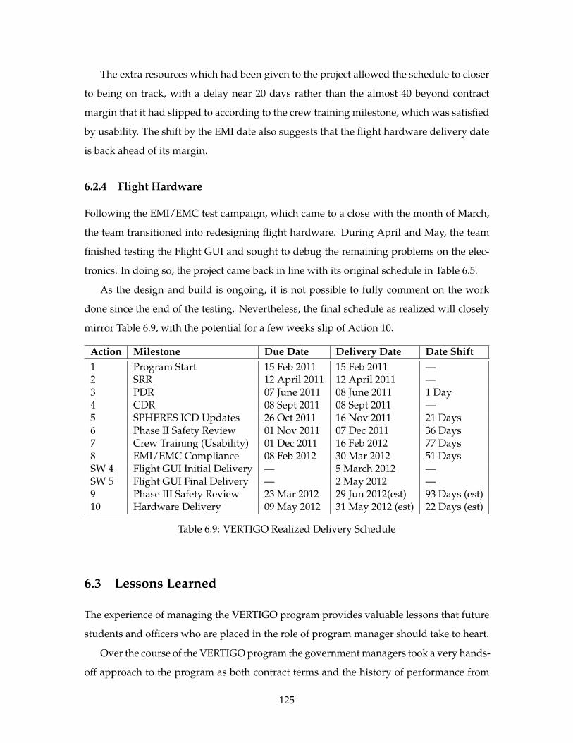
The extra resources which had been given to the project allowed the schedule to closer
to being on track, with a delay near 20 days rather than the almost 40 beyond contract
margin that it had slipped to according to the crew training milestone, which was satisfied
by usability. The shift by the EMI date also suggests that the flight hardware delivery date
is back ahead of its margin.
6.2.4 Flight Hardware
Following the EMI/EMC test campaign, which came to a close with the month of March,
the team transitioned into redesigning flight hardware. During April and May, the team
finished testing the Flight GUI and sought to debug the remaining problems on the elec-
tronics. In doing so, the project came back in line with its original schedule in Table 6.5.
As the design and build is ongoing, it is not possible to fully comment on the work
done since the end of the testing. Nevertheless, the final schedule as realized will closely
mirror Table 6.9, with the potential for a few weeks slip of Action 10.
Action Milestone Due Date Delivery Date Date Shift1 Program Start 15 Feb 2011 15 Feb 2011 —2 SRR 12 April 2011 12 April 2011 —3 PDR 07 June 2011 08 June 2011 1 Day4 CDR 08 Sept 2011 08 Sept 2011 —5 SPHERES ICD Updates 26 Oct 2011 16 Nov 2011 21 Days6 Phase II Safety Review 01 Nov 2011 07 Dec 2011 36 Days7 Crew Training (Usability) 01 Dec 2011 16 Feb 2012 77 Days8 EMI/EMC Compliance 08 Feb 2012 30 Mar 2012 51 DaysSW 4 Flight GUI Initial Delivery — 5 March 2012 —SW 5 Flight GUI Final Delivery — 2 May 2012 —9 Phase III Safety Review 23 Mar 2012 29 Jun 2012(est) 93 Days (est)10 Hardware Delivery 09 May 2012 31 May 2012 (est) 22 Days (est)
Table 6.9: VERTIGO Realized Delivery Schedule
6.3 Lessons Learned
The experience of managing the VERTIGO program provides valuable lessons that future
students and officers who are placed in the role of program manager should take to heart.
Over the course of the VERTIGO program the government managers took a very hands-
off approach to the program as both contract terms and the history of performance from
125
MIT’s Space Systems Laboratory and the subcontractor Aurora Flight Sciences had a strong
history of performance. That history included flights and reflights of dynamics experi-
ments on the Space Shuttle and International Space Station, as well as the original devel-
opment of the SPHERES hardware upon which the VERTIGO hardware would build.
As a result of the flexibility granted by those overseeing the contract for the govern-
ment, your author took two very different approaches to the management of the VERTIGO
program and its staff. These two approaches were motivated by both previous experience
and outside influences including additional projects and guidance from lab leadership.
From it, a few last conclusions can be drawn:
First, for a military officer leading an engineering project in a non-military environ-
ment, leadership needs differ subtly yet substantially from those that training is designed
for. Competence can be assumed for most players, but the resource-constrained environ-
ment makes project management difficult. Other projects also demand time and resources
that are needed to accomplish the mission. In order to gain the needed resources, the
manager must advocate for their project and remain vocal, lest it slip further and further
behind. The flexibility from the higher-level government managers gave the team flexi-
bility, but in the absence of that close oversight, there must be lower-level leadership to
replace it as the driving force behind project success.
Second, a manager must know his or her shortcomings — and they will not be in the
areas you know or expect them to be. The most difficult part of leading the VERTIGO
team was never in those elements with which your author was familiar, like test and op-
erations, but in electronics and software, where experience is less hands-on. This is where
the schedule slip came for VERTIGO. Not because of a failure of the team to do their tasks,
but rather in poor scheduling and time accounting by management. Underestimation is
the result of unfamiliarity.
Finally, it is important to note the impact that additional resources have on forcing
schedule and performance. From the beginning of the project, VERTIGO was considered
a best-effort project by the funding agencies, but not developing sufficient capability was
never an option for the development team. This fixed performance and left schedule and
cost to trade off. The team was able to maintain the schedule by adding resources when
needed. For any manager, there must be a recognition of the project goals, and where slips
are allowable and/or increased investment may be necessary.
126

These three lessons, when combined with the eight themes discussed earlier, allow an
inexperienced project manager to successfully navigate the pitfalls of engineering in an
academic environment. A manager must be ready to Understand, to Build, to Try and Test,
to Grow, to Advocate, to Fail, to develop Depth, and to maintain Margin to guide a program
to a successful conclusion.
127

THIS PAGE INTENTIONALLY LEFT BLANK
128
Chapter 7
Conclusion
The thesis sought to prototype and demonstrate maneuvering and inspection algorithms
for small satellite inspection missions. In particular, it aimed to implement these algo-
rithms on the SPHERES satellite testbed on the ISS in preparation for the eventual launch
of a specialized vision-navigation payload. By analyzing the results from station and com-
paring to simulation, a level of confidence was developed which allowed for more complex
maneuvers to be evaluated.
Further, it sought to develop principles for the project management of small satellite
projects. To do so, the VERTIGO vision-navigation system was used as a case study to
examine what techniques were successful in meeting project goals. By taking stock of
how VERTIGO progressed, these principles were derived from what did and did not work
when applied by program leadership.
7.1 Conclusions
Results showed that the algorithm, when implemented with standard SPHERES controllers,
was able to track the desired state within 10% error. Furthermore, the simulation and sta-
tion results matched within a similar margin, with only a pair of exceptions. By modifying
the mass of the target object, the rotational axes changed. Likewise, rotational rate noise
in simulation was significantly larger than that from station tests. Both of these factors,
however, do not adversely impact the achievement of the mission on station.
Simulation also implies that for a non-parallel inspector and target angular velocities,
the most fuel- and time-efficient inspection paths are planar. For coverage better than a
129
95% threshold, however, it is more efficient to use an estimate of the rotational velocity of
the target object to plan the inspection path.
On the program management side of the VERTIGO program, the principles discussed
have allowed the project to begin to approach its original delivery schedule after a mid-
course slip. With current predictions, it is expected that the maintenance of that manage-
ment approach will result in a nearly-on-schedule delivery of flight hardware with enough
margin to make the scheduled launch to station in Fall 2012.
In the course of the program management described within this thesis, the VERTIGO
team was also able to successfully meet a number of software deadlines. Additionally, the
team has now advanced the design beyond the protoflight stage and is in the midst of
the build of flight hardware. Though time will tell if the team is ultimately successful in
accomplishing its mission goals, signs point to that becoming the case.
7.2 Future Work
First and foremost, flight hardware for VERTIGO must be completed in time to test and
deliver to the Space Test Program, which takes control of the hardware prior to launch.
This will enable the science mission of the program to begin its work in earnest. In addition
to the hardware delivery, there are a handful of other deliverables like a training session
for crew members and safety reviews that are still pending before hardware turnover.
Besides the delivery of the hardware and the associated programmatic deliverables, the
algorithms that were developed for the inspection mission as well as the serial communi-
cation code to interface with SPHERES must be integrated and tested on the satellites. As
demonstrated by the changes that a small additional mass had during the prototype test
session, integration must include adjustment of the controllers to account for changes in
the physical characteristics brought on by attaching the VERTIGO payload.
Also left to be done is the implementation of the software on the station with the new
code to ensure that it meets mission requirements. The code can be validated on the
ground prior to launch, but prior to running the tests on station, those tests are only projec-
tions of what will happen in the microgravity environment, especially with new hardware
in the loop.
The final element of the future work is the ongoing project to inculcate the next gener-
130

ation of MIT program managers with the lessons learned from the program management
of VERTIGO. By passing this corporate knowledge onto future engineers, it is hoped that
the next generation may lead their projects more efficiently and effectively. Eventually,
these lessons should be applied to larger projects and teams to further refine and update
the principles developed within this thesis.
131

Appendices
132
Appendix A
VERTIGO Inspection Maneuver
Codes
A.1 Simple Maneuvers
/* Modified from:
* gsp.c
*
* SPHERES Guest Scientist Program custom source code template.
*
* MIT Space Systems Laboratory
* SPHERES Guest Scientist Program
* http ://ssl.mit.edu/spheres/
*
* Copyright 2005 Massachusetts Institute of Technology
*
* VERTIGO Inspection Maneuver
* Last Update: 5 Oct 2011 by Michael O'Connor*
* ***9 Jul Update :***
* The code was modified to give the TGT object a path to follow during the maneuver
* ***:9 Jul Update ***
*
* ***5 Oct Update :***
* Code modified to have TGT maintain position in Test 1, L-maneuver in Test 2
* ***:5 Oct Update ***
*
*
* *** SPH 1: INSPECTOR (INSP) ***
* *** SPH 2: TARGET (TGT) ***
*
* ***30 Jun Description :***
* The purpose of this test is to demonstrate the 'Phase 1' VERTIGO inspection
maneuver.
* As the Goggles are not yet on station , the relative position/velocity information
is
* simulated using the global metrology system.
*
* The relative information is essentially a transformation from the global frame to
the
133
* body frame of the "Inspector" satellite. In this 2-Sat test , we use the second
SPH
* as the "Target" to be inspected. It begins at a point in the center of the test
volume
* (<0,0,0> on ISS , <0.85,0.55,0.3> on ground). From this initial position , it will
either
* run in a pre -set position and attitude profile or maintain position in the center
of the
* volume.
*
* Each SPH will begin at a location roughly equidistant from the center of the test
volume.
* After 10s of estimator convergence , the "Target" will move to the center of the
test
* volume. The "Inspector" will move to a location ROT_RADIUS away from the
satellite in -X
* with it's expansion port facing the Target. This initial positioning will take 30
s.
* Afterward the Target sphere will spend 5s spinning up to a given rotation speed.
For the
* following 150s, the Inspector will be commanded to rotate based on gyro
information.
* While it rotates , it will translate to keep the Target in the same body -frame
location.
* The Target will follow a proscribed path or maintain its location. The Inspector
should
* still maintain pointing toward the Target throughout this phase.
*
* Test 101: SPH2 (Target) holds position
* Test 102: SPH2 moves in L-shaped path
*
* *** NOTE :***
* It is possible to change the rotation rate , the "center" of the test volume and
the
* radius of the inspection circle by changing the values in the:
* "Change Rates , Center Points , etc here" section
* ***: NOTE ***
*/
/* ----------------------------------------------------------------------------*/
/* Do not modify this section. */
/* ----------------------------------------------------------------------------*/
#include "comm.h"
#include "commands.h"
#include "control.h"
#include "gsp.h"
#include "gsp_task.h"
#include "pads.h"
#include "prop.h"
#include "spheres_constants.h"
#include "spheres_physical_parameters.h"
#include "spheres_types.h"
#include "std_includes.h"
#include "system.h"
#include "util_memory.h"
/* ----------------------------------------------------------------------------*/
/* Modify as desired below this point. */
/* ----------------------------------------------------------------------------*/
#include "ctrl_attitude.h"
#include "ctrl_position.h"
#include "find_state_error.h"
#include "ctrl_mix.h"
#include "math_matrix.h"
#include <math.h>
#include <string.h>
134
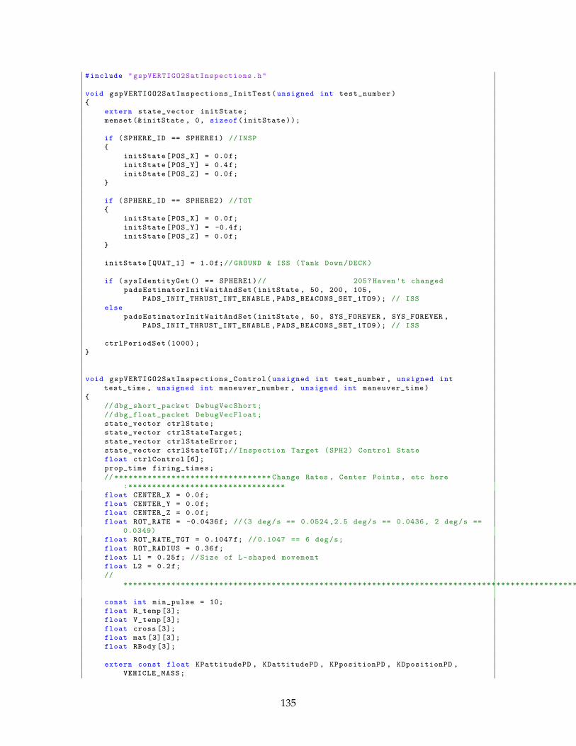
#include "gspVERTIGO2SatInspections.h"
void gspVERTIGO2SatInspections_InitTest(unsigned int test_number)
{
extern state_vector initState;
memset (&initState , 0, sizeof(initState));
if (SPHERE_ID == SPHERE1) //INSP
{
initState[POS_X] = 0.0f;
initState[POS_Y] = 0.4f;
initState[POS_Z] = 0.0f;
}
if (SPHERE_ID == SPHERE2) //TGT
{
initState[POS_X] = 0.0f;
initState[POS_Y] = -0.4f;
initState[POS_Z] = 0.0f;
}
initState[QUAT_1] = 1.0f;// GROUND & ISS (Tank Down/DECK)
if (sysIdentityGet () == SPHERE1)// 205? Haven 't changed
padsEstimatorInitWaitAndSet(initState , 50, 200, 105,
PADS_INIT_THRUST_INT_ENABLE ,PADS_BEACONS_SET_1TO9); // ISS
else
padsEstimatorInitWaitAndSet(initState , 50, SYS_FOREVER , SYS_FOREVER ,
PADS_INIT_THRUST_INT_ENABLE ,PADS_BEACONS_SET_1TO9); // ISS
ctrlPeriodSet (1000);
}
void gspVERTIGO2SatInspections_Control(unsigned int test_number , unsigned int
test_time , unsigned int maneuver_number , unsigned int maneuver_time)
{
// dbg_short_packet DebugVecShort;
// dbg_float_packet DebugVecFloat;
state_vector ctrlState;
state_vector ctrlStateTarget;
state_vector ctrlStateError;
state_vector ctrlStateTGT;// Inspection Target (SPH2) Control State
float ctrlControl [6];
prop_time firing_times;
// ********************************* Change Rates , Center Points , etc here
:*********************************
float CENTER_X = 0.0f;
float CENTER_Y = 0.0f;
float CENTER_Z = 0.0f;
float ROT_RATE = -0.0436f; //(3 deg/s == 0.0524 ,2.5 deg/s == 0.0436 , 2 deg/s ==
0.0349)
float ROT_RATE_TGT = 0.1047f; // 0.1047 == 6 deg/s;
float ROT_RADIUS = 0.36f;
float L1 = 0.25f; //Size of L-shaped movement
float L2 = 0.2f;
//
***************************************************************************************************
const int min_pulse = 10;
float R_temp [3];
float V_temp [3];
float cross [3];
float mat [3][3];
float RBody [3];
extern const float KPattitudePD , KDattitudePD , KPpositionPD , KDpositionPD ,
VEHICLE_MASS;
135
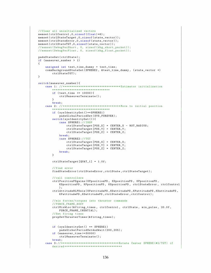
//Clear all uninitialized vectors
memset(ctrlControl ,0,sizeof(float)*6);
memset(ctrlStateTarget ,0,sizeof(state_vector));
memset(ctrlStateError ,0,sizeof(state_vector));
memset(ctrlStateTGT ,0,sizeof(state_vector));
// memset(DebugVecShort , 0, sizeof(dbg_short_packet));
// memset(DebugVecFloat , 0, sizeof(dbg_float_packet));
padsStateGet(ctrlState);
if (maneuver_number > 1)
{
unsigned int test_time_dummy = test_time;
commBackgroundStateGet(SPHERE2 , &test_time_dummy , (state_vector *)
ctrlStateTGT);
}
switch(maneuver_number){
case 1: // ********************************* Estimator initialization
*********************************
if (test_time >= 10000){
ctrlManeuverTerminate ();
}
break;
case 2: // ********************************* Move to initial position
*********************************
if (sysIdentityGet ()== SPHERE1)
padsGlobalPeriodSet(SYS_FOREVER);
switch(sysIdentityGet ()){
case SPHERE1://INSP
ctrlStateTarget[POS_X] = CENTER_X - ROT_RADIUS;
ctrlStateTarget[POS_Y] = CENTER_Y;
ctrlStateTarget[POS_Z] = CENTER_Z;
break;
case SPHERE2://TGT
ctrlStateTarget[POS_X] = CENTER_X;
ctrlStateTarget[POS_Y] = CENTER_Y;
ctrlStateTarget[POS_Z] = CENTER_Z;
break;
}
ctrlStateTarget[QUAT_1] = 1.0f;
//find error
findStateError(ctrlStateError ,ctrlState ,ctrlStateTarget);
//call controllers
ctrlPositionPDgains(KPpositionPD , KDpositionPD , KPpositionPD ,
KDpositionPD , KPpositionPD , KDpositionPD , ctrlStateError , ctrlControl
);
ctrlAttitudeNLPDwie(KPattitudePD ,KDattitudePD ,KPattitudePD ,KDattitudePD ,
KPattitudePD ,KDattitudePD ,ctrlStateError ,ctrlControl);
//mix forces/torques into thruster commands
// FORCE_FRAME_BODY
ctrlMixWLoc (& firing_times , ctrlControl , ctrlState , min_pulse , 20.0f,
FORCE_FRAME_INERTIAL);
//Set firing times
propSetThrusterTimes (& firing_times);
if (sysIdentityGet () == SPHERE1)
padsGlobalPeriodSetAndWait (200 ,205);
if (maneuver_time >=30000)
ctrlManeuverTerminate ();
break;
case 3:// ********************************* Rotate Center SPHERE (#2/ TGT) if
desired *********************************
136
switch(sysIdentityGet ()){
case SPHERE1://INSP
ctrlStateTarget[POS_X] = CENTER_X - ROT_RADIUS;
ctrlStateTarget[POS_Y] = CENTER_Y;
ctrlStateTarget[POS_Z] = CENTER_Z;
break;
case SPHERE2://TGT
//Spin
ctrlStateTarget[RATE_Z] = ROT_RATE_TGT;
ctrlStateTarget[RATE_Y] = ROT_RATE_TGT;// Tumble
ctrlStateTarget[POS_X] = CENTER_X;
ctrlStateTarget[POS_Y] = CENTER_Y;
ctrlStateTarget[POS_Z] = CENTER_Z;
break;
}
ctrlStateTarget[QUAT_1] = 1.0f;
//Estimate , Calculate Control , and Fire Thrusters
findStateError(ctrlStateError ,ctrlState ,ctrlStateTarget);
ctrlPositionPDgains(KPpositionPD , KDpositionPD , KPpositionPD ,
KDpositionPD , KPpositionPD , KDpositionPD , ctrlStateError ,
ctrlControl);
if (sysIdentityGet () == SPHERE1)
ctrlAttitudeNLPDwie(KPattitudePD ,KDattitudePD ,KPattitudePD ,
KDattitudePD ,KPattitudePD ,KDattitudePD ,ctrlStateError ,
ctrlControl);
else
ctrlAttitudeNLPDwie (0,KDattitudePD ,0,KDattitudePD ,0,
KDattitudePD ,ctrlStateError ,ctrlControl);//Use this to
ignore quaternion error from global met
ctrlMixWLoc (& firing_times , ctrlControl , ctrlState , min_pulse ,
20.0f, FORCE_FRAME_INERTIAL);// Changed from 40.0f to 20.0f
propSetThrusterTimes (& firing_times);
if (sysIdentityGet () == SPHERE1)
padsGlobalPeriodSetAndWait (200 ,205);
//if (sysIdentityGet () == SPHERE2)
// padsGlobalPeriodSetAndWait (200 ,205);
if (maneuver_time >=5000)
ctrlManeuverTerminate ();
break;
case 4: // ********************************* Begin Inspector Rotation and
Inspection Maneuver *********************************
if (sysIdentityGet ()== SPHERE1)
{
padsGlobalPeriodSet(SYS_FOREVER);
// Gather Simulated Vision Data
/* ctrlState (current sph state) begins in global frame
* ... convert to body frame:
* POS are in global
* VEL are in global
* QUAT are from global frame to body frame
* RATE are in body
* We will use the quaternions to take the postion and velocity
vectors
* from the global frame to the body frame
*/
//Make measurements relative:
//Moves about point at center of volume (0,0,0)
R_temp [0] = ctrlStateTGT[POS_X] - ctrlState[POS_X];
R_temp [1] = ctrlStateTGT[POS_Y] - ctrlState[POS_Y];
R_temp [2] = ctrlStateTGT[POS_Z] - ctrlState[POS_Z];
//Move to Body Frame
quat2matrixIn(mat , &ctrlState[QUAT_1 ]);//MAT <= rotation matrix
from global to body
137
mathMatVecMult(RBody , (float **)mat , R_temp , 3, 3);
ctrlState[POS_X] = RBody [0];
ctrlState[POS_Y] = RBody [1];
ctrlState[POS_Z] = RBody [2];
//V = Rot*(r ') - wx(Rot(r)))
ctrlState[VEL_X] = ctrlStateTGT[VEL_X] - ctrlState[VEL_X];
ctrlState[VEL_Y] = ctrlStateTGT[VEL_Y] - ctrlState[VEL_Y];
ctrlState[VEL_Z] = ctrlStateTGT[VEL_Z] - ctrlState[VEL_Z];
mathMatVecMult(V_temp , (float **)mat , &ctrlState[VEL_X], 3, 3);
mathVecCross(cross , &ctrlState[RATE_X], &ctrlState[POS_X]);
ctrlState[VEL_X] = V_temp [0] - cross [0];
ctrlState[VEL_Y] = V_temp [1] - cross [1];
ctrlState[VEL_Z] = V_temp [2] - cross [2];
//End Gathering Simulated Vision Data
ctrlStateTarget[POS_X] = ROT_RADIUS;
ctrlStateTarget[RATE_Z] = -ROT_RATE;
//May need to reverse of other maneuvers because of global to body
frame transformation , though QUAT is uncontrolled -for
ctrlStateTarget[QUAT_1] = 1.0f;
//find error
findStateError(ctrlStateError ,ctrlState ,ctrlStateTarget);
//call controllers
ctrlPositionPDgains(KPpositionPD , KDpositionPD , KPpositionPD ,
KDpositionPD , KPpositionPD , KDpositionPD , ctrlStateError ,
ctrlControl);
ctrlAttitudeNLPDwie (0,KDattitudePD ,0,KDattitudePD ,0,KDattitudePD ,
ctrlStateError ,ctrlControl);//Use this to ignore quaternion
error from global met
// Adjust for frame change
ctrlControl [0] *= -1;
ctrlControl [1] *= -1;
ctrlControl [2] *= -1;
// Feedforward Term
ctrlControl [0] += (VEHICLE_MASS*ctrlStateTarget[POS_X]*
ctrlStateTarget[RATE_Z ]* ctrlStateTarget[RATE_Z ]);
//Set firing times , schedule firing
ctrlMixWLoc (& firing_times , ctrlControl , ctrlState , min_pulse ,
20.0f, FORCE_FRAME_BODY);// Changed from 40.0f to 20.0f
propSetThrusterTimes (& firing_times);
}
//If SPH_2 is to follow some path or movement , insert it here:
if (sysIdentityGet () == SPHERE2)
{
if (( maneuver_time > 60000) && (test_number == 2))
ctrlStateTarget[POS_X] = CENTER_X - L2;
else
ctrlStateTarget[POS_X] = CENTER_X;
if (( maneuver_time > 30000) && (test_number == 2))
ctrlStateTarget[POS_Y] = CENTER_Y - L1;
else
ctrlStateTarget[POS_Y] = CENTER_Y;
ctrlStateTarget[QUAT_1] = 1.0f;
ctrlStateTarget[POS_Z] = CENTER_Z;
//find error
findStateError(ctrlStateError ,ctrlState ,ctrlStateTarget);
//call controllers (no attitude control)
138
ctrlPositionPDgains(KPpositionPD , KDpositionPD , KPpositionPD ,
KDpositionPD , KPpositionPD , KDpositionPD , ctrlStateError ,
ctrlControl);
//Set firing times , schedule firing
ctrlMixWLoc (& firing_times , ctrlControl , ctrlState , min_pulse ,
20.0f, FORCE_FRAME_INERTIAL);// Changed from 40.0f to 20.0f
propSetThrusterTimes (& firing_times);
}
if (sysIdentityGet () == SPHERE1)
padsGlobalPeriodSetAndWait (200 ,205);
if (maneuver_time >=150000)
ctrlTestTerminate(TEST_RESULT_NORMAL);
break;
default:
ctrlTestTerminate(TEST_RESULT_ERROR);
break;
}
// DebugPackets
/*
* We want to know:
* 1) Test Time
* 2) Actual Position (Relative)
* 3) Desired Position (Relative)
* 4) Actual Angular Rate
* 5) Desired Angular Rate
* 4) Forces (Body Frame)
* 5) Torques (Body Frame)
*/
/*
//To Debug , in the data file in Matlab , divide by the constant
//in order to get the values in ms , m, and rad/s, respectively
//Time (in tenths of a seconds)
DebugVecShort [0] = (short) (test_time *0.01f);
DebugVecFloat [0] = (float) (test_time *0.01f);
// Actual Relative Position (in 1/10 ths of a mm)
DebugVecShort [1] = (short) (ctrlState[POS_X ]*10000.0f);
DebugVecShort [2] = (short) (ctrlState[POS_Y ]*10000.0f);
DebugVecShort [3] = (short) (ctrlState[POS_Z ]*10000.0f);
// Desired Relative Position (in 1/10 ths of a mm)
DebugVecShort [5] = (short) (ctrlStateTarget[POS_X ]*10000.0f);
DebugVecShort [6] = (short) (ctrlStateTarget[POS_Y ]*10000.0f);
DebugVecShort [7] = (short) (ctrlStateTarget[POS_Z ]*10000.0f);//(
ctrlStateTarget[QUAT_1 ]*100.0f);
// Actual Angular Velocity (in 1/10000 ths of a rad/s)
DebugVecShort [8] = (short) (ctrlState[RATE_X ]*10000.0f);//( ctrlStateTarget[
QUAT_2 ]*100.0f);
DebugVecShort [9] = (short) (ctrlState[RATE_Y ]*10000.0f);//( ctrlStateTarget[
QUAT_3 ]*100.0f);
DebugVecShort [10] = (short) (ctrlState[RATE_Z ]*10000.0f);//( ctrlStateTarget[
QUAT_4 ]*100.0f);
// Desired Angular Velocity (in 1/10000 ths of a rad/s)
DebugVecShort [11] = (short) (ctrlStateTarget[RATE_X ]*10000.0f);
DebugVecShort [12] = (short) (ctrlStateTarget[RATE_Y ]*10000.0f);
DebugVecShort [13] = (short) (ctrlStateTarget[RATE_Z ]*10000.0f);
// Maneuver Number
DebugVecShort [14] = (short) (maneuver_number);
// Commanded Force
DebugVecFloat [1] = ctrlControl[FORCE_X ];
DebugVecFloat [2] = ctrlControl[FORCE_Y ];
DebugVecFloat [3] = ctrlControl[FORCE_Z ];
// Commanded Torque
DebugVecFloat [5] = ctrlControl[TORQUE_X ];
DebugVecFloat [6] = ctrlControl[TORQUE_Y ];
DebugVecFloat [7] = ctrlControl[TORQUE_Z ];
// Send DBG Packets
139

commSendPacket(COMM_CHANNEL_STL ,GROUND ,sysIdentityGet (),
COMM_CMD_DBG_SHORT_SIGNED , (unsigned char *) DebugVecShort , 0);// May end in
COMM_MODE_NO_ACK instead of 0
commSendPacket(COMM_CHANNEL_STL ,GROUND ,sysIdentityGet (), COMM_CMD_DBG_FLOAT , (
unsigned char *) DebugVecFloat , 0);
*/
}
140
A.2 Advanced Maneuvers
/* Modified from :* gsp . c** SPHERES Guest S c i e n t i s t Program custom source code template .** MIT Space Systems Laboratory* SPHERES Guest S c i e n t i s t Program* http :// s s l . mit . edu/spheres/** Copyright 2005 Massachusetts I n s t i t u t e of Technology** VERTIGO 2 Sat Paths Experiment* Last Update : 09 Mar 2012 by Michael O ' Connor* Based o f f of VERTIGO I n s p e c t i o n Maneuver Code* Modif icat ion from 27 Feb to 09 Mar inc ludes :* −Addition of ” Cl oses t Point ” algorithm* −Inc ludes Changing of algorithm from r o t a t i n g and c o n t r o l l i n g t r a n s l a t i o n to
t r a n s l a t i n g* and c o n t r o l l i n g r o t a t i o n** * * * SPH 1 : INSPECTOR ( INSP ) * * ** * * * SPH 2 : TARGET (TGT) * * **** * * * 2 7 Feb 2012 Descr ipt ion : * * *** Test 3 0 1 : SPH2 ( Target ) moves toward INSP , then moves in Z−d i r e c t i o n* Test 3 0 2 : SPH1 ( I n s p e c t o r ) moves in 3−D path* Test 3 0 3 : SPH1 performs 10−min i n s p e c t i o n* Test 3 0 4 : SPH1 i n s p e c t s using SPH2 r o t a t i o n information** Test 3 0 1 : SPH2 ( Target ) moves toward INSP , then moves in Z−d i r e c t i o n* This motion f i n d s the TGT s a t e l l i t e r o t a t i n g in the c e n t e r of the volume . INSP
circumnavigates TGT at* a constant range . TGT w i l l move toward INSP and INSP w i l l compensate to maintain
point ing and range . After* more time , the TGT w i l l move out of the i n s p e c t i o n plane . INSP should compensate by
matching upward motion .** Test 3 0 2 : SPH1 ( I n s p e c t o r ) moves in 3−D path* TGT r o t a t e s in c e n t e r of volume . INSP moves 90 degrees around TGT by r o t a t i n g
about i t s Z a x i s . I t then* r o t a t e s 270 degrees about the Y a x i s u n t i l i t i s between the r o t a t i n g TGT and the DECK
. I t then completes* coverage by r o t a t i n g 90 degrees about Z once more .** Test 3 0 3 : SPH1 performs 10−min i n s p e c t i o n* TGT r o t a t e s in c e n t e r of volume . INSP circumnavigates TGT f o r a period of
approximately 10 minutes . I t* should complete about 2 . 5 ” o r b i t s ” .** Test 3 0 4 : SPH1 i n s p e c t s using SPH2 r o t a t i o n information :* The TGT s a t e l l i t e w i l l r o t a t e in the c e n t e r of the volume . Since v i s i o n can give
r o t a t i o n information ,* we w i l l get r a t e s t a t e information from the TGT . After INSP determines d i r e c t i o n of
spin , INSP w i l l move* to l o c a t i o n perp indicu lar to spin a x i s . I t w i l l s t a r t moving in d i r e c t i o n of TGT spin
a x i s while a l s o* moving around the TGT in a d i r e c t i o n opposi te the spin . The motion in the spin a x i s
d i r e c t i o n w i l l complete* as soon as p o s s i b l e . The motion opposi te the spin d i r e c t i o n should continue u n t i l the
sum of the TGT and* INSP motion sums to 2 pi .* The INSP should then move a n t i p a r a l l e l to the spin a x i s d i r e c t i o n and repeat i t s
observat ions of the
141
* ” southern hemisphere” of the TGT . I t w i l l repeat t h i s and then i n s p e c t the ” equator ”of the TGT .
*** * * *NOTE: * * ** I t i s p o s s i b l e to change the r o t a t i o n rate , the ” c e n t e r ” of the t e s t volume and the* radius of the i n s p e c t i o n c i r c l e by changing the values in the :* ”Change Rates , Center Points , e t c here ” s e c t i o n* * * * :NOTE* * **/
/*−−−−−−−−−−−−−−−−−−−−−−−−−−−−−−−−−−−−−−−−−−−−−−−−−−−−−−−−−−−−−−−−−−−−−−−−−−−−*//* Do not modify t h i s s e c t i o n . *//*−−−−−−−−−−−−−−−−−−−−−−−−−−−−−−−−−−−−−−−−−−−−−−−−−−−−−−−−−−−−−−−−−−−−−−−−−−−−*/
# include ”comm. h”# include ”commands . h”# include ” c o n t r o l . h”# include ”gsp . h”# include ” gsp task . h”# include ”pads . h”# include ”prop . h”# include ” s p h e r e s c o n s t a n t s . h”# include ” spheres phys ica l parameters . h”# include ” spheres types . h”# include ” s t d i n c l u d e s . h”# include ”system . h”# include ” util memory . h”
/*−−−−−−−−−−−−−−−−−−−−−−−−−−−−−−−−−−−−−−−−−−−−−−−−−−−−−−−−−−−−−−−−−−−−−−−−−−−−*//* Modify as des ired below t h i s point . *//*−−−−−−−−−−−−−−−−−−−−−−−−−−−−−−−−−−−−−−−−−−−−−−−−−−−−−−−−−−−−−−−−−−−−−−−−−−−−*/# include ” c t r l a t t i t u d e . h”# include ” c t r l p o s i t i o n . h”# include ” f i n d s t a t e e r r o r . h”# include ” housekeeping internal . h”# include ” housekeeping . h”# include ” c t r l m i x . h”# include ” math matrix . h”# include <math . h># include <s t r i n g . h># include ”gspVERTIGO 2SatPaths . h”
f l o a t throughAngle ;f l o a t maneuverCounter ;i n t rotFlag ;
void gspVERTIGO_2SatPaths_InitTest ( unsigned i n t test_number ){
extern state_vector initState ;memset(&initState , 0 , s i z e o f ( initState ) ) ;
i f ( SPHERE_ID == SPHERE1 ) //INSP{
initState [ POS_X ] = 0 . 0 f ;initState [ POS_Y ] = 0 . 4 f ;initState [ POS_Z ] = 0 . 0 f ;
}
i f ( SPHERE_ID == SPHERE2 ) //TGT{
initState [ POS_X ] = 0 . 0 f ;initState [ POS_Y ] = −0.4f ;initState [ POS_Z ] = 0 . 0 f ;
}
initState [ QUAT_1 ] = 1 . 0 f ; //GROUND & ISS ( Tank Down/DECK)
142
i f ( sysIdentityGet ( ) == SPHERE1 ) // 205?Haven ' t changedpadsEstimatorInitWaitAndSet ( initState , 50 , 200 , 105 , PADS_INIT_THRUST_INT_ENABLE ,
PADS_BEACONS_SET_1TO9 ) ; // ISSe l s e
padsEstimatorInitWaitAndSet ( initState , 50 , SYS_FOREVER , SYS_FOREVER ,PADS_INIT_THRUST_INT_ENABLE , PADS_BEACONS_SET_1TO9 ) ; // ISS
ctrlPeriodSet ( 1 0 0 0 ) ;throughAngle = 0 . 0 f ;maneuverCounter = 0 . 0 f ;
}
void gspVERTIGO_2SatPaths_Control ( unsigned i n t test_number , unsigned i n t test_time ,unsigned i n t maneuver_number , unsigned i n t maneuver_time )
{//dbg short packet DebugVecShort ;// d b g f l o a t p a c k e t DebugVecFloat ;state_vector ctrlState ;state_vector ctrlStateTarget ;state_vector ctrlStateError ;state_vector ctrlStateTGT ; //I n s p e c t i o n Target (SPH2) Control S t a t ef l o a t ctrlControl [ 6 ] ;f l o a t RATE ;f l o a t ROT_RATE_DIR [ 4 ] ;f l o a t vecOut [ 4 ] ;f l o a t TGT_RATE ;prop_time firing_times ;// * * * * * * * * * * * * * * * * * * * * * * * * * * * * * * * * * Change Rates , Center Points , e t c here
: * * * * * * * * * * * * * * * * * * * * * * * * * * * * * * * * *f l o a t CENTER_X = 0 . 0 f ;f l o a t CENTER_Y = 0 . 0 f ;f l o a t CENTER_Z = 0 . 0 f ;f l o a t ROT_RATE = 0 .0262f ; //(3 deg/s == 0 . 0 5 2 4 , 2 . 5 deg/s == 0 . 0 4 3 6 , 2 deg/s ==
0 . 0 3 4 9 , 1 . 5 deg/s == 0 . 0 2 6 2 )f l o a t ROT_RATE_TGT = −0.1047f ; //0 .1047 == 6 deg/s ;f l o a t ROT_RADIUS = 0 . 7 0 f ;f l o a t L1 = 0 . 2 5 f ; //Size of L−shaped movementf l o a t L2 = 0 . 2 0 f ;
//* * * * * * * * * * * * * * * * * * * * * * * * * * * * * * * * * * * * * * * * * * * * * * * * * * * * * * * * * * * * * * * * * * * * * * * * * * * * * * * * * * * * * * * * * * * * * * * * * * *
const i n t min_pulse = 1 0 ;f l o a t MAN4_TIME_LIMIT = 150000 .0f ;
dbg_float_packet DebugVecFloat ;dbg_short_packet DebugVecShort ;
ex tern const f l o a t KPattitudePD , KDattitudePD , KPpositionPD , KDpositionPD ,VEHICLE_MASS ;
memset ( DebugVecFloat , 0 , s i z e o f ( DebugVecFloat ) ) ;memset ( DebugVecShort , 0 , s i z e o f ( DebugVecShort ) ) ;
//Account f o r movement of t a r g e t during t h i s t e s t − t r y to remain in volumei f ( test_number <= 1){
CENTER_Y = −1.0f *L1 ;CENTER_Z = L2 ;
}
//Clear a l l u n i n i t i a l i z e d v e c t o r smemset ( ctrlControl , 0 , s i z e o f ( f l o a t ) * 6 ) ;memset ( ctrlStateTarget , 0 , s i z e o f ( state_vector ) ) ;memset ( ctrlStateError , 0 , s i z e o f ( state_vector ) ) ;memset ( ctrlStateTGT , 0 , s i z e o f ( state_vector ) ) ;//memset ( DebugVecShort , 0 , s i z e o f ( dbg short packet ) ) ;
143
//memset ( DebugVecFloat , 0 , s i z e o f ( d b g f l o a t p a c k e t ) ) ;
padsStateGet ( ctrlState ) ;commBackgroundStateGet ( SPHERE2 , &test_time , ( state_vector * ) ctrlStateTGT ) ;
switch ( maneuver_number ) {case 1 : // * * * * * * * * * * * * * * * * * * * * * * * * * * * * * * * * * * * * * * * * * * * * * * * * * * * * * * * * * * * * * * * * * *
Maneuver 1 : Est imator i n i t i a l i z a t i o n* * * * * * * * * * * * * * * * * * * * * * * * * * * * * * * * * * * * * * * * * * * * * * * * * * * * * * * * * * * * * * * * * *
//Termination a f t e r 10 si f ( maneuver_time >= 10000){
ctrlManeuverTerminate ( ) ;}break ;
case 2 : // * * * * * * * * * * * * * * * * * * * * * * * * * * * * * * * * * * * * * * * * * * * * * * * * * * * * * * * * * * * * * * * * * *Maneuver 2 : Move to i n i t i a l p o s i t i o n* * * * * * * * * * * * * * * * * * * * * * * * * * * * * * * * * * * * * * * * * * * * * * * * * * * * * * * * * * * * * * * * * *
//Termination a f t e r 30 si f ( sysIdentityGet ( ) ==SPHERE1 )
padsGlobalPeriodSet ( SYS_FOREVER ) ;switch ( sysIdentityGet ( ) ) {
case SPHERE1 : //INSPctrlStateTarget [ POS_X ] = CENTER_X − ROT_RADIUS ;ctrlStateTarget [ POS_Y ] = CENTER_Y ;ctrlStateTarget [ POS_Z ] = CENTER_Z ;
break ;case SPHERE2 : //TGT
ctrlStateTarget [ POS_X ] = CENTER_X ;ctrlStateTarget [ POS_Y ] = CENTER_Y ;ctrlStateTarget [ POS_Z ] = CENTER_Z ;
break ;}
//Rotate I n s p e c t o r S a t e l l i t e to show I n i t i a l P o s i t i o n i n g has begun and tod i s t i n g u i s h INSP from TGT
ctrlStateTarget [ QUAT_1 ] = 1 . 0 f ;
//f ind e r r o rfindStateError ( ctrlStateError , ctrlState , ctrlStateTarget ) ;
// c a l l c o n t r o l l e r sctrlPositionPDgains ( KPpositionPD , KDpositionPD , KPpositionPD , KDpositionPD ,
KPpositionPD , KDpositionPD , ctrlStateError , ctrlControl ) ;ctrlAttitudeNLPDwie ( KPattitudePD , KDattitudePD , KPattitudePD , KDattitudePD ,
KPattitudePD , KDattitudePD , ctrlStateError , ctrlControl ) ;
//mix f o r c e s /torques i n t o t h r u s t e r commands//FORCE FRAME BODYctrlMixWLoc(&firing_times , ctrlControl , ctrlState , min_pulse , 2 0 . 0f ,
FORCE_FRAME_INERTIAL ) ;//Set f i r i n g timespropSetThrusterTimes(&firing_times ) ;
i f ( sysIdentityGet ( ) == SPHERE1 )padsGlobalPeriodSetAndWait ( 2 0 0 , 2 0 5 ) ;
i f ( maneuver_time>=30000)ctrlManeuverTerminate ( ) ;
break ;case 3 : // * * * * * * * * * * * * * * * * * * * * * * * * * * * * * * * * * * * * * * * * * * * * * * * * * * * * * * * * * * * * * * * * * *
Maneuver 3 : Rotate Center SPHERE(#2/TGT) i f des ired* * * * * * * * * * * * * * * * * * * * * * * * * * * * * * * * * * * * * * * * * * * * * * * * * * * * * * * * * * * * * * * * * *
//Termination a f t e r 05 sswitch ( sysIdentityGet ( ) ) {
case SPHERE1 : //INSPctrlStateTarget [ POS_X ] = CENTER_X − ROT_RADIUS ;ctrlStateTarget [ POS_Y ] = CENTER_Y ;
144
ctrlStateTarget [ POS_Z ] = CENTER_Z ;break ;case SPHERE2 : //TGT
ctrlStateTarget [ RATE_Z ] = ROT_RATE_TGT ; //SpinctrlStateTarget [ RATE_Y ] = ROT_RATE_TGT ; //Tumblei f ( test_number == 4){
// c t r l S t a t e T a r g e t [RATE Y] = c t r l S t a t e T a r g e t [RATE Y ] / ( 4 . 0 f ) ;ctrlStateTarget [ RATE_Z ] = ctrlStateTarget [ RATE_Z ] / ( 4 . 0 f ) ; // 0 . 0 f ;
}ctrlStateTarget [ POS_X ] = CENTER_X ;ctrlStateTarget [ POS_Y ] = CENTER_Y ;ctrlStateTarget [ POS_Z ] = CENTER_Z ;
break ;}
ctrlStateTarget [ QUAT_1 ] = 1 . 0 f ;
//Estimate , Ca l c u l a te Control , and F i r e ThrustersfindStateError ( ctrlStateError , ctrlState , ctrlStateTarget ) ;ctrlPositionPDgains ( KPpositionPD , KDpositionPD , KPpositionPD ,
KDpositionPD , KPpositionPD , KDpositionPD , ctrlStateError ,ctrlControl ) ;
i f ( sysIdentityGet ( ) == SPHERE1 )ctrlAttitudeNLPDwie ( KPattitudePD , KDattitudePD , KPattitudePD ,
KDattitudePD , KPattitudePD , KDattitudePD , ctrlStateError ,ctrlControl ) ;
e l s ectrlAttitudeNLPDwie ( 0 , KDattitudePD , 0 , KDattitudePD , 0 , KDattitudePD ,
ctrlStateError , ctrlControl ) ; //Use t h i s to ignore quaternione r r o r from globa l met
ctrlMixWLoc(&firing_times , ctrlControl , ctrlState , min_pulse , 2 0 . 0f ,FORCE_FRAME_INERTIAL ) ; //Changed from 4 0 . 0 f to 2 0 . 0 f
propSetThrusterTimes(&firing_times ) ;
i f ( sysIdentityGet ( ) == SPHERE1 )padsGlobalPeriodSetAndWait ( 2 0 0 , 2 0 5 ) ;
// i f ( s y s I d e n t i t y G e t ( ) == SPHERE2)// padsGlobalPeriodSetAndWait ( 2 0 0 , 2 0 5 ) ;i f ( maneuver_time>=5000)
ctrlManeuverTerminate ( ) ;break ;
case 4 : // * * * * * * * * * * * * * * * * * * * * * * * * * * * * * * * * * * * * * * * * * * * * * * * * * * * * * * * * * * * * * * * * * *Maneuver 4 : Begin I n s p e c t o r Rotat ion and I n s p e c t i o n Maneuver* * * * * * * * * * * * * * * * * * * * * * * * * * * * * * * * * * * * * * * * * * * * * * * * * * * * * * * * * * * * * * * * * *
// * * * * * * * * * * * * * * * * * * * * * * * * * * * * * * * * * * * * * * * * * * * * * * * * * * * * * * * * * * * * * * * * * * SPHERE 1 :INSPECTOR* * * * * * * * * * * * * * * * * * * * * * * * * * * * * * * * * * * * * * * * * * * * * * * * * * * * * * * * * * * * * * * * * *
i f ( sysIdentityGet ( ) == SPHERE1 ){
padsGlobalPeriodSet ( SYS_FOREVER ) ;
// * * * * * * * * * * * * * * * * * * * * * * * * * * * * * * * * * * * * * * * * * * * * * * * * * * * * * * * Gather SimulatedVision Data * * * * * * * * * * * * * * * * * * * * * * * * * * * * * * * * * * * * * * * * * * * * * * * * * * * * * * *
changetoBodyFrame(&ctrlStateTGT [ POS_X ] , &ctrlState [ POS_X ] , vecOut ,POSITION_VECTOR ) ;
ctrlState [ POS_X ] = vecOut [ 0 ] ;ctrlState [ POS_Y ] = vecOut [ 1 ] ;ctrlState [ POS_Z ] = vecOut [ 2 ] ;changetoBodyFrame(&ctrlStateTGT [ POS_X ] , &ctrlState [ POS_X ] , vecOut ,
VELOCITY_VECTOR ) ;ctrlState [ VEL_X ] = vecOut [ 0 ] ;ctrlState [ VEL_Y ] = vecOut [ 1 ] ;ctrlState [ VEL_Z ] = vecOut [ 2 ] ;changetoBodyFrame(&ctrlStateTGT [ POS_X ] , &ctrlState [ POS_X ] , vecOut ,
ROTATION_VECTOR ) ;ROT_RATE_DIR [ 0 ] = vecOut [ 0 ] ;
145
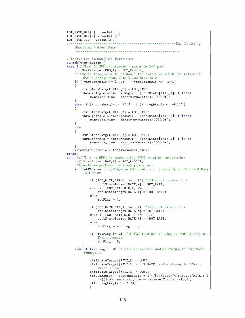
ROT_RATE_DIR [ 1 ] = vecOut [ 1 ] ;ROT_RATE_DIR [ 2 ] = vecOut [ 2 ] ;ROT_RATE_TGT = vecOut [ 3 ] ;// * * * * * * * * * * * * * * * * * * * * * * * * * * * * * * * * * * * * * * * * * * * * * * * * * * * * * * * End Gathering
Simulated Vision Data* * * * * * * * * * * * * * * * * * * * * * * * * * * * * * * * * * * * * * * * * * * * * * * * * * * * * * *
//I n s p e c t i o n Motion/Path Parametersswitch ( test_number ) {case 2 : //Test 2 : SPH1 ( I n s p e c t o r ) moves in 3−D path
ctrlStateTarget [ POS_X ] = ROT_RADIUS ;// Use an i n t e g r a t o r to es t imate the points a t which the r o t a t i o n s
should change from Z to Y and back to Zi f ( ( throughAngle >= 2*PI ) | | ( throughAngle <= −2*PI ) ){
ctrlStateTarget [ RATE_Z ] = ROT_RATE ;throughAngle = throughAngle + ( ctrlState [ RATE_Z ] * ( ( f l o a t )
maneuver_time − maneuverCounter ) /1000.0f ) ;}e l s e i f ( ( throughAngle >= PI/2) | | ( throughAngle <= −PI/2) ){
ctrlStateTarget [ RATE_Y ] = ROT_RATE ;throughAngle = throughAngle + ( ctrlState [ RATE_Y ] * ( ( f l o a t )
maneuver_time − maneuverCounter ) /1000.0f ) ;}e l s e{
ctrlStateTarget [ RATE_Z ] = ROT_RATE ;throughAngle = throughAngle + ( ctrlState [ RATE_Z ] * ( ( f l o a t )
maneuver_time − maneuverCounter ) /1000.0f ) ;}maneuverCounter = ( f l o a t ) maneuver_time ;
break ;case 4 : //Test 4 : SPH1 i n s p e c t s using SPH2 r o t a t i o n information
ctrlStateTarget [ POS_X ] = ROT_RADIUS ;//Time/Coverage−based movement procedures :i f ( rotFlag == 0) //Align so TGT spin a x i s i s roughly in INSP ' s Z−Body
D i r e c t i o n{
i f ( ROT_RATE_DIR [ 0 ] >= . 0 1 f ) //Align i f e r r o r s in XctrlStateTarget [ RATE_Y ] = ROT_RATE ;
e l s e i f ( ROT_RATE_DIR [ 0 ] <= −.01f )ctrlStateTarget [ RATE_Y ] = −ROT_RATE ;
e l s erotFlag = 1 ;
i f ( ROT_RATE_DIR [ 1 ] >= . 0 1 ) //Align i f e r r o r s in YctrlStateTarget [ RATE_X ] = ROT_RATE ;
e l s e i f ( ROT_RATE_DIR [ 1 ] <= −.01f )ctrlStateTarget [ RATE_X ] = −ROT_RATE ;
e l s erotFlag = rotFlag + 1 ;
i f ( rotFlag != 2 ) // I f TGT r o t a t i o n i s al igned with Z a x i s ofINSP , proceedrotFlag = 0 ;
}e l s e i f ( rotFlag == 2) //Begin i n s p e c t i o n motion moving to ”Northern
Hemisphere”{
ctrlStateTarget [ RATE_Z ] = 0 . 0 f ;ctrlStateTarget [ RATE_Y ] = ROT_RATE ; //For Moving to ”North
Pole ” of TGTctrlStateTarget [ RATE_X ] = 0 . 0 f ;throughAngle = throughAngle + ( ( ( f l o a t ) fabs ( ctrlState [ RATE_Y ] )
) * ( ( f l o a t ) maneuver_time − maneuverCounter ) /1000) ;i f ( throughAngle >= PI/4){
146
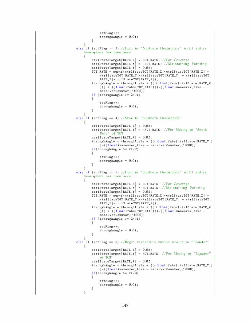
rotFlag++;throughAngle = 0 . 0 f ;
}}
e l s e i f ( rotFlag == 3) //Hold in ”Northern Hemisphere” u n t i l e n t i r ehemisphere has been seen .{
ctrlStateTarget [ RATE_Z ] = ROT_RATE ; //For CoveragectrlStateTarget [ RATE_X ] = −ROT_RATE ; //Maintaining Point ingctrlStateTarget [ RATE_Y ] = 0 . 0 f ;TGT_RATE = sqrtf ( ctrlStateTGT [ RATE_X ] * ctrlStateTGT [ RATE_X ] +
ctrlStateTGT [ RATE_Y ] * ctrlStateTGT [ RATE_Y ] + ctrlStateTGT [RATE_Z ] * ctrlStateTGT [ RATE_Z ] ) ;
throughAngle = throughAngle + ( ( ( ( f l o a t ) fabs ( ctrlState [ RATE_Z] ) ) + ( ( f l o a t ) fabs ( TGT_RATE ) ) ) * ( ( f l o a t ) maneuver_time −maneuverCounter ) /1000) ;
i f ( throughAngle >= 2*PI ){
rotFlag++;throughAngle = 0 . 0 f ;
}}
e l s e i f ( rotFlag == 4) //Move to ” Southern Hemisphere”{
ctrlStateTarget [ RATE_Z ] = 0 . 0 f ;ctrlStateTarget [ RATE_Y ] = −ROT_RATE ; //For Moving to ”South
Pole ” of TGTctrlStateTarget [ RATE_X ] = 0 . 0 f ;throughAngle = throughAngle + ( ( ( f l o a t ) fabs ( ctrlState [ RATE_Y ] )
) * ( ( f l o a t ) maneuver_time − maneuverCounter ) /1000) ;i f ( throughAngle >= PI/2){
rotFlag++;throughAngle = 0 . 0 f ;
}}
e l s e i f ( rotFlag == 5) //Hold in ” Southern Hemisphere” u n t i l e n t i r ehemisphere has been seen .{
ctrlStateTarget [ RATE_Z ] = ROT_RATE ; //For CoveragectrlStateTarget [ RATE_X ] = ROT_RATE ; //Maintaining Point ingctrlStateTarget [ RATE_Y ] = 0 . 0 f ;TGT_RATE = sqrtf ( ctrlStateTGT [ RATE_X ] * ctrlStateTGT [ RATE_X ] +
ctrlStateTGT [ RATE_Y ] * ctrlStateTGT [ RATE_Y ] + ctrlStateTGT [RATE_Z ] * ctrlStateTGT [ RATE_Z ] ) ;
throughAngle = throughAngle + ( ( ( ( f l o a t ) fabs ( ctrlState [ RATE_Z] ) ) + ( ( f l o a t ) fabs ( TGT_RATE ) ) ) * ( ( f l o a t ) maneuver_time −maneuverCounter ) /1000) ;
i f ( throughAngle >= 2*PI ){
rotFlag++;throughAngle = 0 . 0 f ;
}}
e l s e i f ( rotFlag == 6) //Begin i n s p e c t i o n motion moving to ” Equator ”{
ctrlStateTarget [ RATE_Z ] = 0 . 0 f ;ctrlStateTarget [ RATE_Y ] = ROT_RATE ; //For Moving to ” Equator ”
of TGTctrlStateTarget [ RATE_X ] = 0 . 0 f ;throughAngle = throughAngle + ( ( ( f l o a t ) fabs ( ctrlState [ RATE_Y ] )
) * ( ( f l o a t ) maneuver_time − maneuverCounter ) /1000) ;i f ( throughAngle >= PI/4){
rotFlag++;throughAngle = 0 . 0 f ;
}}
147
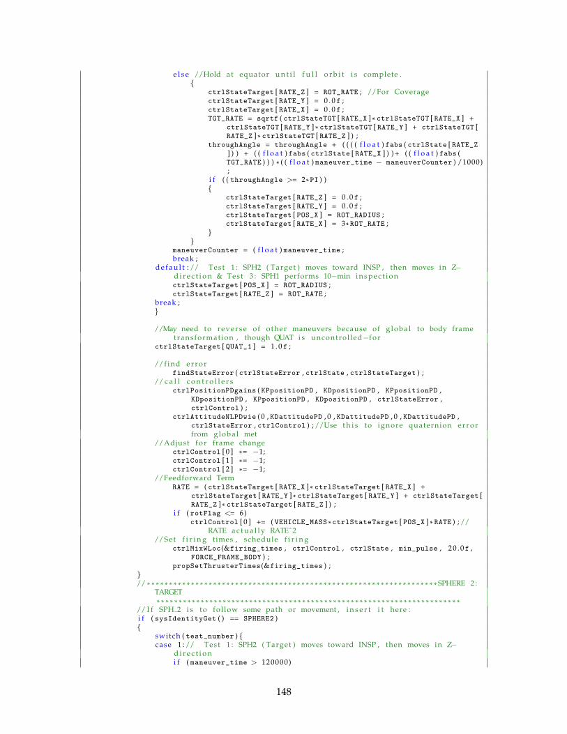
e l s e //Hold at equator u n t i l f u l l o r b i t i s complete .{
ctrlStateTarget [ RATE_Z ] = ROT_RATE ; //For CoveragectrlStateTarget [ RATE_Y ] = 0 . 0 f ;ctrlStateTarget [ RATE_X ] = 0 . 0 f ;TGT_RATE = sqrtf ( ctrlStateTGT [ RATE_X ] * ctrlStateTGT [ RATE_X ] +
ctrlStateTGT [ RATE_Y ] * ctrlStateTGT [ RATE_Y ] + ctrlStateTGT [RATE_Z ] * ctrlStateTGT [ RATE_Z ] ) ;
throughAngle = throughAngle + ( ( ( ( f l o a t ) fabs ( ctrlState [ RATE_Z] ) ) + ( ( f l o a t ) fabs ( ctrlState [ RATE_X ] ) ) + ( ( f l o a t ) fabs (TGT_RATE ) ) ) * ( ( f l o a t ) maneuver_time − maneuverCounter ) /1000);
i f ( ( throughAngle >= 2*PI ) ){
ctrlStateTarget [ RATE_Z ] = 0 . 0 f ;ctrlStateTarget [ RATE_Y ] = 0 . 0 f ;ctrlStateTarget [ POS_X ] = ROT_RADIUS ;ctrlStateTarget [ RATE_X ] = 3* ROT_RATE ;
}}
maneuverCounter = ( f l o a t ) maneuver_time ;break ;
d e f a u l t : // Test 1 : SPH2 ( Target ) moves toward INSP , then moves in Z−d i r e c t i o n & Test 3 : SPH1 performs 10−min i n s p e c t i o nctrlStateTarget [ POS_X ] = ROT_RADIUS ;ctrlStateTarget [ RATE_Z ] = ROT_RATE ;
break ;}
//May need to reverse of other maneuvers because of g loba l to body frametransformation , though QUAT i s uncontrol led−f o r
ctrlStateTarget [ QUAT_1 ] = 1 . 0 f ;
//f ind e r r o rfindStateError ( ctrlStateError , ctrlState , ctrlStateTarget ) ;
// c a l l c o n t r o l l e r sctrlPositionPDgains ( KPpositionPD , KDpositionPD , KPpositionPD ,
KDpositionPD , KPpositionPD , KDpositionPD , ctrlStateError ,ctrlControl ) ;
ctrlAttitudeNLPDwie ( 0 , KDattitudePD , 0 , KDattitudePD , 0 , KDattitudePD ,ctrlStateError , ctrlControl ) ; //Use t h i s to ignore quaternion e r r o rfrom globa l met
//Adjust f o r frame changectrlControl [ 0 ] *= −1;ctrlControl [ 1 ] *= −1;ctrlControl [ 2 ] *= −1;
//Feedforward TermRATE = ( ctrlStateTarget [ RATE_X ] * ctrlStateTarget [ RATE_X ] +
ctrlStateTarget [ RATE_Y ] * ctrlStateTarget [ RATE_Y ] + ctrlStateTarget [RATE_Z ] * ctrlStateTarget [ RATE_Z ] ) ;
i f ( rotFlag <= 6)ctrlControl [ 0 ] += ( VEHICLE_MASS * ctrlStateTarget [ POS_X ] * RATE ) ; //
RATE a c t u a l l y RATEˆ2//Set f i r i n g times , schedule f i r i n g
ctrlMixWLoc(&firing_times , ctrlControl , ctrlState , min_pulse , 2 0 . 0f ,FORCE_FRAME_BODY ) ;
propSetThrusterTimes(&firing_times ) ;}// * * * * * * * * * * * * * * * * * * * * * * * * * * * * * * * * * * * * * * * * * * * * * * * * * * * * * * * * * * * * * * * * * * SPHERE 2 :
TARGET* * * * * * * * * * * * * * * * * * * * * * * * * * * * * * * * * * * * * * * * * * * * * * * * * * * * * * * * * * * * * * * * * * * * *
// I f SPH 2 i s to fol low some path or movement , i n s e r t i t here :i f ( sysIdentityGet ( ) == SPHERE2 ){
switch ( test_number ) {case 1 : // Test 1 : SPH2 ( Target ) moves toward INSP , then moves in Z−
d i r e c t i o ni f ( maneuver_time > 120000)
148
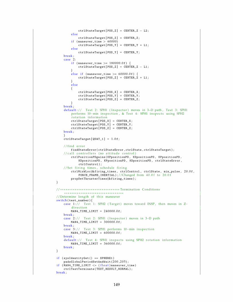
ctrlStateTarget [ POS_Z ] = CENTER_Z − L2 ;e l s e
ctrlStateTarget [ POS_Z ] = CENTER_Z ;i f ( maneuver_time > 60000)
ctrlStateTarget [ POS_Y ] = CENTER_Y + L1 ;e l s e
ctrlStateTarget [ POS_Y ] = CENTER_Y ;break ;case 2 :
i f ( maneuver_time >= 180000 .0f ) {ctrlStateTarget [ POS_Z ] = CENTER_Z − L1 ;
}e l s e i f ( maneuver_time >= 60000 .0f ) {
ctrlStateTarget [ POS_Z ] = CENTER_Z + L1 ;}e l s e{
ctrlStateTarget [ POS_X ] = CENTER_X ;ctrlStateTarget [ POS_Y ] = CENTER_Y ;ctrlStateTarget [ POS_Z ] = CENTER_Z ;
}break ;d e f a u l t : // Test 2 : SPH1 ( I n s p e c t o r ) moves in 3−D path , Test 3 : SPH1
performs 10−min inspect ion , & Test 4 : SPH1 i n s p e c t s using SPH2r o t a t i o n informationctrlStateTarget [ POS_X ] = CENTER_X ;ctrlStateTarget [ POS_Y ] = CENTER_Y ;ctrlStateTarget [ POS_Z ] = CENTER_Z ;
break ;}ctrlStateTarget [ QUAT_1 ] = 1 . 0 f ;
//f ind e r r o rfindStateError ( ctrlStateError , ctrlState , ctrlStateTarget ) ;
// c a l l c o n t r o l l e r s ( no a t t i t u d e c o n t r o l )ctrlPositionPDgains ( KPpositionPD , KDpositionPD , KPpositionPD ,
KDpositionPD , KPpositionPD , KDpositionPD , ctrlStateError ,ctrlControl ) ;
//Set f i r i n g times , schedule f i r i n gctrlMixWLoc(&firing_times , ctrlControl , ctrlState , min_pulse , 2 0 . 0f ,
FORCE_FRAME_INERTIAL ) ; //Changed from 4 0 . 0 f to 2 0 . 0 fpropSetThrusterTimes(&firing_times ) ;
}
// * * * * * * * * * * * * * * * * * * * * * * * * * * * * * * * * * Termination Conditions* * * * * * * * * * * * * * * * * * * * * * * * * * * * * * * * *
//Determine length of t h i s maneuverswitch ( test_number ) {
case 1 : // Test 1 : SPH2 ( Target ) moves toward INSP , then moves in Z−d i r e c t i o nMAN4_TIME_LIMIT = 240000 .0f ;
break ;case 2 : // Test 2 : SPH1 ( I n s p e c t o r ) moves in 3−D path
MAN4_TIME_LIMIT = 300000 .0f ;break ;case 3 : // Test 3 : SPH1 performs 10−min i n s p e c t i o n
MAN4_TIME_LIMIT = 600000 .0f ;break ;d e f a u l t : // Test 4 : SPH1 i n s p e c t s using SPH2 r o t a t i o n information
MAN4_TIME_LIMIT = 360000 .0f ;break ;
}
i f ( sysIdentityGet ( ) == SPHERE1 )padsGlobalPeriodSetAndWait ( 2 0 0 , 2 0 5 ) ;
i f ( MAN4_TIME_LIMIT <= ( f l o a t ) maneuver_time )ctrlTestTerminate ( TEST_RESULT_NORMAL ) ;
break ;
149
d e f a u l t :ctrlTestTerminate ( TEST_RESULT_ERROR ) ;
break ;}
//%%%%%%%%%%%%%%%% DEBUG %%%%%%%%%%%%%%%%
DebugVecFloat [ 0 ] = ctrlState [ POS_X ] ;DebugVecFloat [ 1 ] = ctrlState [ POS_Y ] ;DebugVecFloat [ 2 ] = ctrlState [ POS_Z ] ;DebugVecFloat [ 3 ] = ctrlState [ VEL_X ] ;DebugVecFloat [ 4 ] = ctrlState [ VEL_Y ] ;DebugVecFloat [ 5 ] = ctrlState [ VEL_Z ] ;DebugVecFloat [ 6 ] = ( f l o a t ) test_time/1000;DebugVecFloat [ 7 ] = ( f l o a t ) maneuver_time/1000;commSendPacket ( COMM_CHANNEL_STL , GROUND , 0 , COMM_CMD_DBG_FLOAT , ( unsigned char * )
DebugVecFloat , 0 ) ;
DebugVecShort [ 0 ] = ( shor t ) maneuver_number ;DebugVecShort [ 1 ] = ( shor t ) ( ctrlStateError [ POS_X ] * 1 0 0 0 0 ) ;DebugVecShort [ 2 ] = ( shor t ) ( ctrlStateError [ POS_Y ] * 1 0 0 0 0 ) ;DebugVecShort [ 3 ] = ( shor t ) ( ctrlStateError [ POS_Z ] * 1 0 0 0 0 ) ;DebugVecShort [ 4 ] = ( shor t ) ( ctrlStateError [ RATE_X ] * 1 0 0 0 0 ) ;DebugVecShort [ 5 ] = ( shor t ) ( ctrlStateError [ RATE_Y ] * 1 0 0 0 0 ) ;DebugVecShort [ 6 ] = ( shor t ) ( ctrlStateError [ RATE_Z ] * 1 0 0 0 0 ) ;commSendPacket ( COMM_CHANNEL_STL , GROUND , 0 , COMM_CMD_DBG_SHORT_SIGNED , ( unsigned
char * ) DebugVecShort , 0 ) ;
}
void changetoBodyFrame ( state_vector TargetState , state_vector InspectorState , f l o a t *vectorOut , unsigned i n t vectorType )
{/* T a r g e t S t a t e and I n s p e c t o r S t a t e begins in g loba l frame* . . . convert to body frame :* POS are in g loba l* VEL are in g loba l* QUAT are from globa l frame to body frame* RATE are in body* We w i l l use the quaternions to take the post ion and v e l o c i t y v e c t o r s* from the globa l frame to the body frame*/f l o a t R_temp [ 3 ] ;f l o a t RBody [ 3 ] ;f l o a t cross [ 3 ] ;f l o a t V_temp [ 3 ] ;f l o a t mat [ 3 ] [ 3 ] ;
switch ( vectorType ) {case POSITION_VECTOR :
//Make measurements r e l a t i v e ://Moves about point a t c e n t e r of volume ( 0 , 0 , 0 )R_temp [ 0 ] = TargetState [ POS_X ] − InspectorState [ POS_X ] ;R_temp [ 1 ] = TargetState [ POS_Y ] − InspectorState [ POS_Y ] ;R_temp [ 2 ] = TargetState [ POS_Z ] − InspectorState [ POS_Z ] ;//Move to INSP Body Framequat2matrixIn ( mat , &InspectorState [ QUAT_1 ] ) ; //MAT <= r o t a t i o n matrix from globa l
to INSP bodymathMatVecMult ( RBody , ( f l o a t * * ) mat , R_temp , 3 , 3 ) ;vectorOut [ 0 ] = RBody [ 0 ] ; //POS XvectorOut [ 1 ] = RBody [ 1 ] ; //POS YvectorOut [ 2 ] = RBody [ 2 ] ; //POS Zbreak ;
case VELOCITY_VECTOR ://V = Rot * ( r ' ) − wx( Rot ( r ) ) )InspectorState [ VEL_X ] = TargetState [ VEL_X ] − InspectorState [ VEL_X ] ;InspectorState [ VEL_Y ] = TargetState [ VEL_Y ] − InspectorState [ VEL_Y ] ;InspectorState [ VEL_Z ] = TargetState [ VEL_Z ] − InspectorState [ VEL_Z ] ;
150
mathMatVecMult ( V_temp , ( f l o a t * * ) mat , &InspectorState [ VEL_X ] , 3 , 3 ) ;mathVecCross ( cross , &InspectorState [ RATE_X ] , &InspectorState [ POS_X ] ) ;vectorOut [ 0 ] = V_temp [ 0 ] − cross [ 0 ] ; //VEL XvectorOut [ 1 ] = V_temp [ 1 ] − cross [ 1 ] ; //VEL YvectorOut [ 2 ] = V_temp [ 2 ] − cross [ 2 ] ; //VEL Zbreak ;
case ACCEL_VECTOR :vectorOut [ 0 ] = 0 . 0 f ;vectorOut [ 1 ] = 0 . 0 f ;vectorOut [ 2 ] = 0 . 0 f ;break ;
case ROTATION_VECTOR ://Move TGT Rot in TGT Body to INSP BodyR_temp [ 0 ] = TargetState [ RATE_X ] ; //Get TGT Rotat ion Rates in TGT Body FrameR_temp [ 1 ] = TargetState [ RATE_Y ] ;R_temp [ 2 ] = TargetState [ RATE_Z ] ;quat2matrixOut ( mat , &TargetState [ QUAT_1 ] ) ; //MAT <= r o t a t i o n matrix from TGT Body
to GlobalmathMatVecMult ( RBody , ( f l o a t * * ) mat , R_temp , 3 , 3 ) ; //TGT Body to GlobalR_temp [ 0 ] = RBody [ 0 ] ;R_temp [ 1 ] = RBody [ 1 ] ;R_temp [ 2 ] = RBody [ 2 ] ;memset ( RBody , 0 , s i z e o f ( f l o a t ) * 3 ) ;quat2matrixIn ( mat , &InspectorState [ QUAT_1 ] ) ; //MAT <= r o t a t i o n matrix from globa l
to INSP bodymathMatVecMult ( RBody , ( f l o a t * * ) mat , R_temp , 3 , 3 ) ; //Global to INSP Body//vectorOut = ROT RATE DIR[0−2]vectorOut [ 0 ] = RBody [ 0 ] ; //XvectorOut [ 1 ] = RBody [ 1 ] ; //YvectorOut [ 2 ] = RBody [ 2 ] ; //Z//Find Magnitude//ROT RATE TGTvectorOut [ 3 ] = ( f l o a t ) sqrt ( vectorOut [ 0 ] * vectorOut [ 0 ] + vectorOut [ 1 ] * vectorOut [ 1 ] +
vectorOut [ 2 ] * vectorOut [ 2 ] ) ;break ;
d e f a u l t :ctrlTestTerminate ( 1 3 ) ; //ERROR: I n c o r r e c t c a l l to changetoBodyFramebreak ;
}}
151
A.3 Example Code using Video Data
/* Modified from :* gsp . c** SPHERES Guest S c i e n t i s t Program custom source code template .** MIT Space Systems Laboratory* SPHERES Guest S c i e n t i s t Program* http :// s s l . mit . edu/spheres/** Copyright 2005 Massachusetts I n s t i t u t e of Technology** VERTIGO 2 Sat Paths Experiment* Last Update : 09 Apri l 2012 by Michael O ' Connor :* −I n t e g r a t i o n of S e r i a l Comm & r e a l video information i n t o code* Update : 09 Mar 2012 by Michael O ' Connor :* −Addition of ” Cl oses t Point ” algorithm* −Inc ludes Changing of algorithm from r o t a t i n g and c o n t r o l l i n g t r a n s l a t i o n to
t r a n s l a t i n g* and c o n t r o l l i n g r o t a t i o n* Update : 27 Feb 2012 by Michael O ' Connor** * * * SPH 1 : INSPECTOR ( INSP ) * * ** * * * SPH 2 : TARGET (TGT) * * *** * * * Test Descr ip t ions : * * *** Test 2 0 1 : SPH2 ( Target ) moves toward INSP , then moves in Z−d i r e c t i o n* Test 2 0 2 : SPH1 ( I n s p e c t o r ) moves in 3−D path* Test 2 0 3 : SPH1 performs 10−min i n s p e c t i o n* Test 2 0 4 : SPH1 i n s p e c t s using SPH2 r o t a t i o n information** Longer d e s c r i p t i o n s a v a i l a b l e in previous vers ions of code ( pre−09 Apri l updates ) .** * * *NOTE: * * ** I t i s p o s s i b l e to change the r o t a t i o n rate , the ” c e n t e r ” of the t e s t volume and the* radius of the i n s p e c t i o n c i r c l e by changing the values in the :* ”Change Rates , Center Points , e t c here ” s e c t i o n*/
/*−−−−−−−−−−−−−−−−−−−−−−−−−−−−−−−−−−−−−−−−−−−−−−−−−−−−−−−−−−−−−−−−−−−−−−−−−−−−*//* Do not modify t h i s s e c t i o n . *//*−−−−−−−−−−−−−−−−−−−−−−−−−−−−−−−−−−−−−−−−−−−−−−−−−−−−−−−−−−−−−−−−−−−−−−−−−−−−*/
# include ”comm. h”# include ”commands . h”# include ” c o n t r o l . h”# include ”gsp . h”# include ” gsp task . h”# include ”pads . h”# include ”prop . h”# include ” s p h e r e s c o n s t a n t s . h”# include ” spheres phys ica l parameters . h”# include ” spheres types . h”# include ” s t d i n c l u d e s . h”# include ”system . h”# include ” util memory . h”# include ” exp v2 . h”
/*−−−−−−−−−−−−−−−−−−−−−−−−−−−−−−−−−−−−−−−−−−−−−−−−−−−−−−−−−−−−−−−−−−−−−−−−−−−−*//* Modify as des ired below t h i s point . *//*−−−−−−−−−−−−−−−−−−−−−−−−−−−−−−−−−−−−−−−−−−−−−−−−−−−−−−−−−−−−−−−−−−−−−−−−−−−−*/# include ” c t r l a t t i t u d e . h”# include ” c t r l p o s i t i o n . h”# include ” f i n d s t a t e e r r o r . h”
152
# include ” housekeeping internal . h”# include ” housekeeping . h”# include ” c t r l m i x . h”# include ” math matrix . h”# include ” smt335async . h”# include ” comm internal . h”# include ” g s u t i l t h r t i m e s . h”# include ”gspVERTIGO 2SatPaths . h”# include <math . h># include <s t r i n g . h>
// * * * * * * * * * * * BEGINNING OF COMM DEFINITIONS * * * * * * * * * * *//# = Sphere Comm . . . A = Test S t a r t /Stop . . . B = Watchdog . . .//C = Terminate . . . D = FORCE/TORQUE . . . E = Target Info . . .//F = Misc# def ine START BYTE 0xA7# def ine FROM SPHERES 0x01# def ine FROM GOGGLES 0x02# def ine WATCHDOG REQUEST 0xB1# def ine WATCHDOG REPLY 0xB2# def ine TERMINATE TEST 0xC1# def ine SYNC TEST 0x91# def ine START TEST 0xA3# def ine FORCES TORQUES 0xD1# def ine TGT POSITION 0xE1# def ine WATCHDOG LIMIT 3# def ine ANY GOGGLES 0x40# def ine SPHERE ID REQUEST 0xA2# def ine max length 255
i n t watchdog_flag ;f l o a t forces [ 3 ] ;f l o a t torques [ 3 ] ;f l o a t position [ 3 ] ;f l o a t velocity [ 3 ] ;unsigned char packet_buffer [ max_length ] ;i n t packet_buffer_length = 0 ;i n t initTest = 0 ;i n t GogglesAttached = 0 ;// * * * * * * * * * * *END OF COMM DEFINITIONS * * * * * * * * * * *// * * * * * * * * * * * BEGINNING OF MANEUVER DEFINITIONS * * * * * * * * * * *f l o a t throughAngle ;f l o a t maneuverCounter ;i n t rotFlag ;// * * * * * * * * * * *END OF MANEUVER DEFINITIONS * * * * * * * * * * *// * * * * * * * * * * * BEGINNING OF COMM STRUCT DEFINITIONS * * * * * * * * * * *typedef s t r u c t {
unsigned char return_code ;} msg_terminate_test ;
typedef s t r u c t {unsigned char to ;unsigned char from ;unsigned char ID ;unsigned char test_number ;
} msg_start_test ;
typedef s t r u c t {f l o a t forces [ 3 ] ;f l o a t torques [ 3 ] ;
} msg_body_forces_torques ;
typedef s t r u c t {f l o a t xyzPos [ 3 ] ;f l o a t xyzVel [ 3 ] ;
} msg_body_tgt_location ;
typedef s t r u c t {
153
unsigned char to ;unsigned char from ;unsigned char ID ;unsigned char spheresLogicID ;unsigned i n t programID ;
} msg_spheres_id ;
typedef s t r u c t {unsigned char startByte ;unsigned char length ;unsigned char from ;unsigned char ID ;
} msg_header ;// * * * * * * * * * * *END OF COMM STRUCT DEFINITIONS * * * * * * * * * * *
void gspVERTIGO_2SatPaths_InitTest ( unsigned i n t test_number ){
extern state_vector initState ;// * * * * * * * * * * * BEGINNING OF COMM DEFINITIONS * * * * * * * * * * *msg_start_test msgStart ;msgStart . to = ANY_GOGGLES ;msgStart . from = commHWAddrGet ( ) ;msgStart . ID = START_TEST ;msgStart . test_number = ( unsigned char ) test_number ;expv2_uart_send ( SERIALPORT_DAEMON , s i z e o f ( msgStart ) , ( unsigned char * ) &msgStart ) ;
initTest = 1 ;
memset ( forces , 0 , s i z e o f ( f l o a t ) * 3 ) ;memset ( torques , 0 , s i z e o f ( f l o a t ) * 3 ) ;watchdog_flag = 0 ;// * * * * * * * * * * *END OF COMM DECLARATIONS * * * * * * * * * * *memset(&initState , 0 , s i z e o f ( initState ) ) ;
i f ( SPHERE_ID == SPHERE1 ) //INSP{
initState [ POS_X ] = 0 . 0 f ;initState [ POS_Y ] = 0 . 4 f ;initState [ POS_Z ] = 0 . 0 f ;
}
i f ( SPHERE_ID == SPHERE2 ) //TGT{
initState [ POS_X ] = 0 . 0 f ;initState [ POS_Y ] = −0.4f ;initState [ POS_Z ] = 0 . 0 f ;
}
initState [ QUAT_1 ] = 1 . 0 f ; //GROUND & ISS ( Tank Down/DECK)
i f ( sysIdentityGet ( ) == SPHERE1 ) // 205?Haven ' t changedpadsEstimatorInitWaitAndSet ( initState , 50 , 200 , 105 , PADS_INIT_THRUST_INT_ENABLE ,
PADS_BEACONS_SET_1TO9 ) ; // ISSe l s e
padsEstimatorInitWaitAndSet ( initState , 50 , SYS_FOREVER , SYS_FOREVER ,PADS_INIT_THRUST_INT_ENABLE , PADS_BEACONS_SET_1TO9 ) ; // ISS
ctrlPeriodSet ( 1 0 0 0 ) ;throughAngle = 0 . 0 f ;maneuverCounter = 0 . 0 f ;
}
void gspVERTIGO_2SatPaths_Control ( unsigned i n t test_number , unsigned i n t test_time ,unsigned i n t maneuver_number , unsigned i n t maneuver_time )
{
154
extern const f l o a t KPattitudePD , KDattitudePD , KPpositionPD , KDpositionPD ,VEHICLE_MASS ;
//dbg short packet DebugVecShort ;// d b g f l o a t p a c k e t DebugVecFloat ;state_vector ctrlState ; //Actual S t a t estate_vector ctrlStateTarget ; //Desired S t a t estate_vector ctrlStateError ;state_vector ctrlStateTGT ; //I n s p e c t i o n Target (SPH2) Control S t a t ef l o a t ctrlControl [ 6 ] ;f l o a t RATE ;f l o a t ROT_RATE_DIR [ 4 ] ;f l o a t vecOut [ 4 ] ;f l o a t TGT_RATE ;dbg_float_packet DebugVecFloat ;dbg_short_packet DebugVecShort ;dbg_ushort_packet DebugVecUShort ;prop_time firing_times ;// * * * * * * * * * * * * * * * * * * * * * * * * * * * * * * * * * * Change Rates , Center Points , e t c here
: * * * * * * * * * * * * * * * * * * * * * * * * * * * * * * * * * *f l o a t CENTER_X = 0 . 0 f ;f l o a t CENTER_Y = 0 . 0 f ;f l o a t CENTER_Z = 0 . 0 f ;f l o a t ROT_RATE = 0 .0262f ; //(3 deg/s == 0 . 0 5 2 4 , 2 . 5 deg/s == 0 . 0 4 3 6 , 2 deg/s ==
0 . 0 3 4 9 , 1 . 5 deg/s == 0 . 0 2 6 2 )f l o a t ROT_RATE_TGT = −0.1047f ; //0 .1047 == 6 deg/s ;f l o a t ROT_RADIUS = 0 . 7 0 f ;f l o a t L1 = 0 . 2 5 f ; //Size of L−shaped movementf l o a t L2 = 0 . 2 0 f ;
//* * * * * * * * * * * * * * * * * * * * * * * * * * * * * * * * * * * * * * * * * * * * * * * * * * * * * * * * * * * * * * * * * * * * * * * * * * * * * * * * * * * * * * * * * * * * * * * * * * *
const i n t min_pulse = 1 0 ;f l o a t MAN4_TIME_LIMIT = 150000 .0f ;// * * * * * * * * * * *MESSAGE TYPE DECLARATIONS * * * * * * * * * * *msg_header msgTP ;msg_header msg ;msgTP . startByte = START_BYTE ;msgTP . from = FROM_SPHERES ;msgTP . length = 0 ;msgTP . ID = WATCHDOG_REQUEST ;// * * * * * * * * * * *END MESSAGE TYPE DECLARATIONS * * * * * * * * * * *
memset ( DebugVecFloat , 0 , s i z e o f ( DebugVecFloat ) ) ;memset ( DebugVecShort , 0 , s i z e o f ( DebugVecShort ) ) ;memset ( DebugVecUShort , 0 , s i z e o f ( DebugVecUShort ) ) ;
//Account f o r movement of t a r g e t during t h i s t e s t − t r y to remain in volumei f ( test_number <= 1){
CENTER_Y = −1.0f *L1 ;CENTER_Z = L2 ;
}
//Clear a l l u n i n i t i a l i z e d v e c t o r smemset ( ctrlControl , 0 , s i z e o f ( f l o a t ) * 6 ) ;memset ( ctrlStateTarget , 0 , s i z e o f ( state_vector ) ) ;memset ( ctrlStateError , 0 , s i z e o f ( state_vector ) ) ;memset ( ctrlStateTGT , 0 , s i z e o f ( state_vector ) ) ;//memset ( DebugVecShort , 0 , s i z e o f ( dbg short packet ) ) ;//memset ( DebugVecFloat , 0 , s i z e o f ( d b g f l o a t p a c k e t ) ) ;
padsStateGet ( ctrlState ) ;//commBackgroundStateGet (SPHERE2 , &t e s t t i m e , ( s t a t e v e c t o r * ) c t r lS ta teTGT ) ;ctrlStateTGT [ QUAT_1 ] = 1 ;ctrlStateTGT [ RATE_Z ] = ROT_RATE_TGT ;
155
//Check to see i f WD f l a g was s e t ( to 0 ) ; i f i t = 1 , end t e s ti f ( watchdog_flag >= WATCHDOG_LIMIT ){
initTest = 0 ;ctrlTestTerminate ( RESULT_PAYLOAD_ERROR ) ;
}e l s e i f ( ( test_time % 5000) < 1000){
watchdog_flag++;}
switch ( maneuver_number ) {case 1 : // * * * * * * * * * * * * * * * * * * * * * * * * * * * * * * * * * * Maneuver 1 : Est imator i n i t i a l i z a t i o n
* * * * * * * * * * * * * * * * * * * * * * * * * * * * * * * * * *//Termination a f t e r 10 si f ( maneuver_time >= 10000){
ctrlManeuverTerminate ( ) ;}e l s e i f ( ( maneuver_time >= 5000) && ( maneuver_time <= 7000) ) // i n i t i a l i z e
Goggles{
// ( i n i t T e s t <= 2)msg . startByte = START_BYTE ;msg . from = FROM_SPHERES ;msg . length = 0 ;msg . ID = SYNC_TEST ;expv2_uart_send ( SERIALPORT_TESTPROG , s i z e o f ( msg ) , ( unsigned char * ) &msg ) ;
initTest++;}//Check watchdogi f ( ( test_time % 5000) < 1000){
expv2_uart_send ( SERIALPORT_TESTPROG , s i z e o f ( msgTP ) , ( unsigned char * ) &msgTP );
}break ;
case 2 : // * * * * * * * * * * * * * * * * * * * * * * * * * * * * * * * * * * Maneuver 2 : Move to i n i t i a l p o s i t i o n* * * * * * * * * * * * * * * * * * * * * * * * * * * * * * * * * *
//Termination a f t e r 30 si f ( sysIdentityGet ( ) ==SPHERE1 )
padsGlobalPeriodSet ( SYS_FOREVER ) ;switch ( sysIdentityGet ( ) ) {
case SPHERE1 : //INSPctrlStateTarget [ POS_X ] = CENTER_X − ROT_RADIUS ;ctrlStateTarget [ POS_Y ] = CENTER_Y ;ctrlStateTarget [ POS_Z ] = CENTER_Z ;
break ;case SPHERE2 : //TGT
ctrlStateTarget [ POS_X ] = CENTER_X ;ctrlStateTarget [ POS_Y ] = CENTER_Y ;ctrlStateTarget [ POS_Z ] = CENTER_Z ;
break ;}
//Rotate I n s p e c t o r S a t e l l i t e to show I n i t i a l P o s i t i o n i n g has begun and tod i s t i n g u i s h INSP from TGT
ctrlStateTarget [ QUAT_1 ] = 1 . 0 f ;
//f ind e r r o rfindStateError ( ctrlStateError , ctrlState , ctrlStateTarget ) ;
// c a l l c o n t r o l l e r sctrlPositionPDgains ( KPpositionPD , KDpositionPD , KPpositionPD , KDpositionPD ,
KPpositionPD , KDpositionPD , ctrlStateError , ctrlControl ) ;
156
ctrlAttitudeNLPDwie ( KPattitudePD , KDattitudePD , KPattitudePD , KDattitudePD ,KPattitudePD , KDattitudePD , ctrlStateError , ctrlControl ) ;
i f ( ( test_number == 5) && ( sysIdentityGet ( ) == SPHERE1 ) ){
ctrlControl [ FORCE_X ] = forces [ 0 ] ;ctrlControl [ FORCE_Y ] = forces [ 1 ] ;ctrlControl [ FORCE_Z ] = forces [ 2 ] ;ctrlControl [ TORQUE_X ] = torques [ 0 ] ;ctrlControl [ TORQUE_Y ] = torques [ 1 ] ;ctrlControl [ TORQUE_Z ] = torques [ 2 ] ;ctrlMixWLoc(&firing_times , ctrlControl , ctrlState , min_pulse , 2 0 . 0f ,
FORCE_FRAME_BODY ) ;}e l s e{//mix f o r c e s /torques i n t o t h r u s t e r commands//FORCE FRAME BODYctrlMixWLoc(&firing_times , ctrlControl , ctrlState , min_pulse , 2 0 . 0f ,
FORCE_FRAME_INERTIAL ) ;}//Set f i r i n g timespropSetThrusterTimes(&firing_times ) ;memset ( forces , 0 , 3 * s i z e o f ( f l o a t ) ) ;memset ( torques , 0 , 3 * s i z e o f ( f l o a t ) ) ;//Check watchdogi f ( ( test_time % 5000) < 1000){
expv2_uart_send ( SERIALPORT_TESTPROG , s i z e o f ( msgTP ) , ( unsigned char * ) &msgTP );
}i f ( sysIdentityGet ( ) == SPHERE1 )
padsGlobalPeriodSetAndWait ( 2 0 0 , 2 0 5 ) ;i f ( maneuver_time>=30000)
ctrlManeuverTerminate ( ) ;break ;
case 3 : // * * * * * * * * * * * * * * * * * * * * * * * * * * * * * * * * * * Maneuver 3 : Rotate Center SPHERE(#2/TGT) i f des ired * * * * * * * * * * * * * * * * * * * * * * * * * * * * * * * * * *//Termination a f t e r 05 sswitch ( sysIdentityGet ( ) ) {
case SPHERE1 : //INSPctrlStateTarget [ POS_X ] = CENTER_X − ROT_RADIUS ;ctrlStateTarget [ POS_Y ] = CENTER_Y ;ctrlStateTarget [ POS_Z ] = CENTER_Z ;
break ;case SPHERE2 : //TGT
ctrlStateTarget [ RATE_Z ] = ROT_RATE_TGT ; //SpinctrlStateTarget [ RATE_Y ] = ROT_RATE_TGT ; //Tumblei f ( test_number == 4){
// c t r l S t a t e T a r g e t [RATE Y] = c t r l S t a t e T a r g e t [RATE Y ] / ( 4 . 0 f ) ;ctrlStateTarget [ RATE_Z ] = ctrlStateTarget [ RATE_Z ] / ( 4 . 0 f ) ; // 0 . 0 f ;
}ctrlStateTarget [ POS_X ] = CENTER_X ;ctrlStateTarget [ POS_Y ] = CENTER_Y ;ctrlStateTarget [ POS_Z ] = CENTER_Z ;
break ;}
ctrlStateTarget [ QUAT_1 ] = 1 . 0 f ;
//Estimate , Ca l c u l a te Control , and F i r e ThrustersfindStateError ( ctrlStateError , ctrlState , ctrlStateTarget ) ;ctrlPositionPDgains ( KPpositionPD , KDpositionPD , KPpositionPD ,
KDpositionPD , KPpositionPD , KDpositionPD , ctrlStateError ,ctrlControl ) ;
i f ( sysIdentityGet ( ) == SPHERE1 )ctrlAttitudeNLPDwie ( KPattitudePD , KDattitudePD , KPattitudePD ,
KDattitudePD , KPattitudePD , KDattitudePD , ctrlStateError ,
157
ctrlControl ) ;e l s e
ctrlAttitudeNLPDwie ( 0 , KDattitudePD , 0 , KDattitudePD , 0 , KDattitudePD ,ctrlStateError , ctrlControl ) ; //Use t h i s to ignore quaternione r r o r from globa l met
i f ( test_number == 5){
ctrlControl [ FORCE_X ] = forces [ 0 ] ;ctrlControl [ FORCE_Y ] = forces [ 1 ] ;ctrlControl [ FORCE_Z ] = forces [ 2 ] ;ctrlControl [ TORQUE_X ] = torques [ 0 ] ;ctrlControl [ TORQUE_Y ] = torques [ 1 ] ;ctrlControl [ TORQUE_Z ] = torques [ 2 ] ;ctrlMixWLoc(&firing_times , ctrlControl , ctrlState , min_pulse , 2 0 . 0
f , FORCE_FRAME_BODY ) ;}e l s e{
ctrlMixWLoc(&firing_times , ctrlControl , ctrlState , min_pulse , 2 0 . 0f , FORCE_FRAME_INERTIAL ) ; //Changed from 4 0 . 0 f to 2 0 . 0 f
}propSetThrusterTimes(&firing_times ) ;memset ( forces , 0 , 3 * s i z e o f ( f l o a t ) ) ;memset ( torques , 0 , 3 * s i z e o f ( f l o a t ) ) ;
//Check watchdogi f ( ( test_time % 5000) < 1000){
expv2_uart_send ( SERIALPORT_TESTPROG , s i z e o f ( msgTP ) , ( unsigned char * ) &msgTP );
}i f ( sysIdentityGet ( ) == SPHERE1 )
padsGlobalPeriodSetAndWait ( 2 0 0 , 2 0 5 ) ;// i f ( s y s I d e n t i t y G e t ( ) == SPHERE2)// padsGlobalPeriodSetAndWait ( 2 0 0 , 2 0 5 ) ;i f ( maneuver_time>=5000)
ctrlManeuverTerminate ( ) ;break ;
case 4 : // * * * * * * * * * * * * * * * * * * * * * * * * * * * * * * * * * * Maneuver 4 : Begin I n s p e c t o r Rotat ionand I n s p e c t i o n Maneuver * * * * * * * * * * * * * * * * * * * * * * * * * * * * * * * * * *// * * * * * * * * * * * * * * * * * * * * * * * * * * * * * * * * * * SPHERE 1 : INSPECTOR
* * * * * * * * * * * * * * * * * * * * * * * * * * * * * * * * * *i f ( sysIdentityGet ( ) == SPHERE1 ){
padsGlobalPeriodSet ( SYS_FOREVER ) ;
i f ( GogglesAttached == 0){// * * * * * * * * * * * * * * * * * * * * * * * * * * * * * * * * * * Gather Simulated Vision Data
* * * * * * * * * * * * * * * * * * * * * * * * * * * * * * * * * *changetoBodyFrame(&ctrlStateTGT [ POS_X ] , &ctrlState [ POS_X ] , vecOut ,
POSITION_VECTOR ) ;ctrlState [ POS_X ] = vecOut [ 0 ] ;ctrlState [ POS_Y ] = vecOut [ 1 ] ;ctrlState [ POS_Z ] = vecOut [ 2 ] ;changetoBodyFrame(&ctrlStateTGT [ POS_X ] , &ctrlState [ POS_X ] , vecOut ,
VELOCITY_VECTOR ) ;ctrlState [ VEL_X ] = vecOut [ 0 ] ;ctrlState [ VEL_Y ] = vecOut [ 1 ] ;ctrlState [ VEL_Z ] = vecOut [ 2 ] ;changetoBodyFrame(&ctrlStateTGT [ POS_X ] , &ctrlState [ POS_X ] , vecOut ,
ROTATION_VECTOR ) ;ROT_RATE_DIR [ 0 ] = vecOut [ 0 ] ;ROT_RATE_DIR [ 1 ] = vecOut [ 1 ] ;ROT_RATE_DIR [ 2 ] = vecOut [ 2 ] ;ROT_RATE_TGT = vecOut [ 3 ] ;
158
// * * * * * * * * * * * * * * * * * * * * * * * * * * * * * * * * * * End Gathering Simulated Vision Data* * * * * * * * * * * * * * * * * * * * * * * * * * * * * * * * * *
}e l s e{// * * * * * * * * * * * * * * * * * * * * * * * * * * * * * * * * * * Gather Actual Vision Data
* * * * * * * * * * * * * * * * * * * * * * * * * * * * * * * * * *ctrlState [ POS_X ] = position [ POS_Z ] + 0 . 2 3 4 ; //Move from camera frame to SPH
body framectrlState [ POS_Y ] = −position [ POS_X ] + 0 . 0 4 5 ;ctrlState [ POS_Z ] = −position [ POS_Y ] + 0 . 0 3 0 ;ctrlState [ VEL_X ] = velocity [ 2 ] ;ctrlState [ VEL_Y ] = velocity [ 0 ] ;ctrlState [ VEL_Z ] = velocity [ 1 ] ;changetoBodyFrame(&ctrlStateTGT [ POS_X ] , &ctrlState [ POS_X ] , vecOut ,
ROTATION_VECTOR ) ;ROT_RATE_DIR [ 0 ] = vecOut [ 0 ] ;ROT_RATE_DIR [ 1 ] = vecOut [ 1 ] ;ROT_RATE_DIR [ 2 ] = vecOut [ 2 ] ;ROT_RATE_TGT = vecOut [ 3 ] ;// * * * * * * * * * * * * * * * * * * * * * * * * * * * * * * * * * * End Gathering Actual Vision Data
* * * * * * * * * * * * * * * * * * * * * * * * * * * * * * * * * *}
//I n s p e c t i o n Motion/Path Parametersswitch ( test_number ) {case 2 : //Test 2 : SPH1 ( I n s p e c t o r ) moves in 3−D path
ctrlStateTarget [ POS_X ] = ROT_RADIUS ;// Use an i n t e g r a t o r to es t imate the points a t which the r o t a t i o n s
should change from Z to Y and back to Zi f ( ( throughAngle >= 2*PI ) | | ( throughAngle <= −2*PI ) ){
ctrlStateTarget [ RATE_Z ] = ROT_RATE ;throughAngle = throughAngle + ( ctrlState [ RATE_Z ] * ( ( f l o a t )
maneuver_time − maneuverCounter ) /1000.0f ) ;}e l s e i f ( ( throughAngle >= PI/2) | | ( throughAngle <= −PI/2) ){
ctrlStateTarget [ RATE_Y ] = ROT_RATE ;throughAngle = throughAngle + ( ctrlState [ RATE_Y ] * ( ( f l o a t )
maneuver_time − maneuverCounter ) /1000.0f ) ;}e l s e{
ctrlStateTarget [ RATE_Z ] = ROT_RATE ;throughAngle = throughAngle + ( ctrlState [ RATE_Z ] * ( ( f l o a t )
maneuver_time − maneuverCounter ) /1000.0f ) ;}maneuverCounter = ( f l o a t ) maneuver_time ;
break ;case 4 : //Test 4 : SPH1 i n s p e c t s using SPH2 r o t a t i o n information
ctrlStateTarget [ POS_X ] = ROT_RADIUS ;//Time/Coverage−based movement procedures :i f ( rotFlag == 0) //Align so TGT spin a x i s i s roughly in INSP ' s Z−Body
D i r e c t i o n{
i f ( ROT_RATE_DIR [ 0 ] >= . 0 1 f ) //Align i f e r r o r s in XctrlStateTarget [ RATE_Y ] = ROT_RATE ;
e l s e i f ( ROT_RATE_DIR [ 0 ] <= −.01f )ctrlStateTarget [ RATE_Y ] = −ROT_RATE ;
e l s erotFlag = 1 ;
i f ( ROT_RATE_DIR [ 1 ] >= . 0 1 ) //Align i f e r r o r s in YctrlStateTarget [ RATE_X ] = ROT_RATE ;
e l s e i f ( ROT_RATE_DIR [ 1 ] <= −.01f )ctrlStateTarget [ RATE_X ] = −ROT_RATE ;
e l s e
159
rotFlag = rotFlag + 1 ;
i f ( rotFlag != 2 ) // I f TGT r o t a t i o n i s al igned with Z a x i s ofINSP , proceedrotFlag = 0 ;
}e l s e i f ( rotFlag == 2) //Begin i n s p e c t i o n motion moving to ”Northern
Hemisphere”{
ctrlStateTarget [ RATE_Z ] = 0 . 0 f ;ctrlStateTarget [ RATE_Y ] = ROT_RATE ; //For Moving to ”North
Pole ” of TGTctrlStateTarget [ RATE_X ] = 0 . 0 f ;throughAngle = throughAngle + ( ( ( f l o a t ) fabs ( ctrlState [ RATE_Y ] )
) * ( ( f l o a t ) maneuver_time − maneuverCounter ) /1000) ;i f ( throughAngle >= PI/4){
rotFlag++;throughAngle = 0 . 0 f ;
}}
e l s e i f ( rotFlag == 3) //Hold in ”Northern Hemisphere” u n t i l e n t i r ehemisphere has been seen .{
ctrlStateTarget [ RATE_Z ] = ROT_RATE ; //For CoveragectrlStateTarget [ RATE_X ] = −ROT_RATE ; //Maintaining Point ingctrlStateTarget [ RATE_Y ] = 0 . 0 f ;TGT_RATE = sqrtf ( ctrlStateTGT [ RATE_X ] * ctrlStateTGT [ RATE_X ] +
ctrlStateTGT [ RATE_Y ] * ctrlStateTGT [ RATE_Y ] + ctrlStateTGT [RATE_Z ] * ctrlStateTGT [ RATE_Z ] ) ;
throughAngle = throughAngle + ( ( ( ( f l o a t ) fabs ( ctrlState [ RATE_Z] ) ) + ( ( f l o a t ) fabs ( TGT_RATE ) ) ) * ( ( f l o a t ) maneuver_time −maneuverCounter ) /1000) ;
i f ( throughAngle >= 2*PI ){
rotFlag++;throughAngle = 0 . 0 f ;
}}
e l s e i f ( rotFlag == 4) //Move to ” Southern Hemisphere”{
ctrlStateTarget [ RATE_Z ] = 0 . 0 f ;ctrlStateTarget [ RATE_Y ] = −ROT_RATE ; //For Moving to ”South
Pole ” of TGTctrlStateTarget [ RATE_X ] = 0 . 0 f ;throughAngle = throughAngle + ( ( ( f l o a t ) fabs ( ctrlState [ RATE_Y ] )
) * ( ( f l o a t ) maneuver_time − maneuverCounter ) /1000) ;i f ( throughAngle >= PI/2){
rotFlag++;throughAngle = 0 . 0 f ;
}}
e l s e i f ( rotFlag == 5) //Hold in ” Southern Hemisphere” u n t i l e n t i r ehemisphere has been seen .{
ctrlStateTarget [ RATE_Z ] = ROT_RATE ; //For CoveragectrlStateTarget [ RATE_X ] = ROT_RATE ; //Maintaining Point ingctrlStateTarget [ RATE_Y ] = 0 . 0 f ;TGT_RATE = sqrtf ( ctrlStateTGT [ RATE_X ] * ctrlStateTGT [ RATE_X ] +
ctrlStateTGT [ RATE_Y ] * ctrlStateTGT [ RATE_Y ] + ctrlStateTGT [RATE_Z ] * ctrlStateTGT [ RATE_Z ] ) ;
throughAngle = throughAngle + ( ( ( ( f l o a t ) fabs ( ctrlState [ RATE_Z] ) ) + ( ( f l o a t ) fabs ( TGT_RATE ) ) ) * ( ( f l o a t ) maneuver_time −maneuverCounter ) /1000) ;
i f ( throughAngle >= 2*PI ){
rotFlag++;
160
throughAngle = 0 . 0 f ;}
}e l s e i f ( rotFlag == 6) //Begin i n s p e c t i o n motion moving to ” Equator ”
{ctrlStateTarget [ RATE_Z ] = 0 . 0 f ;ctrlStateTarget [ RATE_Y ] = ROT_RATE ; //For Moving to ” Equator ”
of TGTctrlStateTarget [ RATE_X ] = 0 . 0 f ;throughAngle = throughAngle + ( ( ( f l o a t ) fabs ( ctrlState [ RATE_Y ] )
) * ( ( f l o a t ) maneuver_time − maneuverCounter ) /1000) ;i f ( throughAngle >= PI/4){
rotFlag++;throughAngle = 0 . 0 f ;
}}
e l s e //Hold at equator u n t i l f u l l o r b i t i s complete .{
ctrlStateTarget [ RATE_Z ] = ROT_RATE ; //For CoveragectrlStateTarget [ RATE_Y ] = 0 . 0 f ;ctrlStateTarget [ RATE_X ] = 0 . 0 f ;TGT_RATE = sqrtf ( ctrlStateTGT [ RATE_X ] * ctrlStateTGT [ RATE_X ] +
ctrlStateTGT [ RATE_Y ] * ctrlStateTGT [ RATE_Y ] + ctrlStateTGT [RATE_Z ] * ctrlStateTGT [ RATE_Z ] ) ;
throughAngle = throughAngle + ( ( ( ( f l o a t ) fabs ( ctrlState [ RATE_Z] ) ) + ( ( f l o a t ) fabs ( ctrlState [ RATE_X ] ) ) + ( ( f l o a t ) fabs (TGT_RATE ) ) ) * ( ( f l o a t ) maneuver_time − maneuverCounter ) /1000);
i f ( ( throughAngle >= 2*PI ) ){
ctrlStateTarget [ RATE_Z ] = 0 . 0 f ;ctrlStateTarget [ RATE_Y ] = 0 . 0 f ;ctrlStateTarget [ POS_X ] = ROT_RADIUS ;ctrlStateTarget [ RATE_X ] = 3* ROT_RATE ;
}}
maneuverCounter = ( f l o a t ) maneuver_time ;break ;
d e f a u l t : // Test 1 : SPH2 ( Target ) moves toward INSP , then moves in Z−d i r e c t i o n & Test 3 : SPH1 performs 10−min i n s p e c t i o nctrlStateTarget [ POS_X ] = ROT_RADIUS ;ctrlStateTarget [ RATE_Z ] = ROT_RATE ;
break ;}
//May need to reverse of other maneuvers because of g loba l to body frametransformation , though QUAT i s uncontrol led−f o r
ctrlStateTarget [ QUAT_1 ] = 1 . 0 f ;
//f ind e r r o rfindStateError ( ctrlStateError , ctrlState , ctrlStateTarget ) ;
// c a l l c o n t r o l l e r sctrlPositionPDgains ( KPpositionPD , KDpositionPD , KPpositionPD ,
KDpositionPD , KPpositionPD , KDpositionPD , ctrlStateError ,ctrlControl ) ;
ctrlAttitudeNLPDwie ( 0 , KDattitudePD , 0 , KDattitudePD , 0 , KDattitudePD ,ctrlStateError , ctrlControl ) ; //Use t h i s to ignore quaternion e r r o rfrom globa l met
//Adjust f o r frame changectrlControl [ 0 ] *= −1;ctrlControl [ 1 ] *= −1;ctrlControl [ 2 ] *= −1;
//Feedforward TermRATE = ( ctrlStateTarget [ RATE_X ] * ctrlStateTarget [ RATE_X ] +
ctrlStateTarget [ RATE_Y ] * ctrlStateTarget [ RATE_Y ] + ctrlStateTarget [RATE_Z ] * ctrlStateTarget [ RATE_Z ] ) ;
i f ( rotFlag <= 6)
161
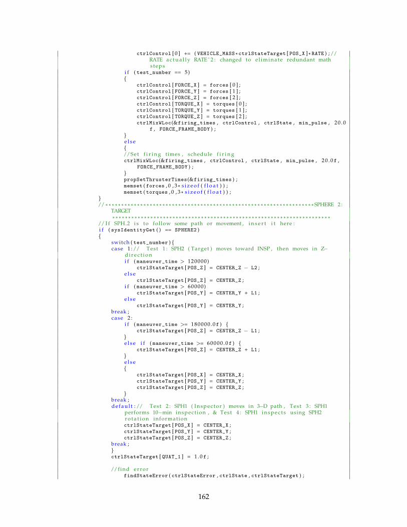
ctrlControl [ 0 ] += ( VEHICLE_MASS * ctrlStateTarget [ POS_X ] * RATE ) ; //RATE a c t u a l l y RATEˆ 2 : changed to e l i m i n a t e redundant maths teps
i f ( test_number == 5){
ctrlControl [ FORCE_X ] = forces [ 0 ] ;ctrlControl [ FORCE_Y ] = forces [ 1 ] ;ctrlControl [ FORCE_Z ] = forces [ 2 ] ;ctrlControl [ TORQUE_X ] = torques [ 0 ] ;ctrlControl [ TORQUE_Y ] = torques [ 1 ] ;ctrlControl [ TORQUE_Z ] = torques [ 2 ] ;ctrlMixWLoc(&firing_times , ctrlControl , ctrlState , min_pulse , 2 0 . 0
f , FORCE_FRAME_BODY ) ;}e l s e{//Set f i r i n g times , schedule f i r i n gctrlMixWLoc(&firing_times , ctrlControl , ctrlState , min_pulse , 2 0 . 0f ,
FORCE_FRAME_BODY ) ;}propSetThrusterTimes(&firing_times ) ;memset ( forces , 0 , 3 * s i z e o f ( f l o a t ) ) ;memset ( torques , 0 , 3 * s i z e o f ( f l o a t ) ) ;
}// * * * * * * * * * * * * * * * * * * * * * * * * * * * * * * * * * * * * * * * * * * * * * * * * * * * * * * * * * * * * * * * * * * SPHERE 2 :
TARGET* * * * * * * * * * * * * * * * * * * * * * * * * * * * * * * * * * * * * * * * * * * * * * * * * * * * * * * * * * * * * * * * * * * * *
// I f SPH 2 i s to fol low some path or movement , i n s e r t i t here :i f ( sysIdentityGet ( ) == SPHERE2 ){
switch ( test_number ) {case 1 : // Test 1 : SPH2 ( Target ) moves toward INSP , then moves in Z−
d i r e c t i o ni f ( maneuver_time > 120000)
ctrlStateTarget [ POS_Z ] = CENTER_Z − L2 ;e l s e
ctrlStateTarget [ POS_Z ] = CENTER_Z ;i f ( maneuver_time > 60000)
ctrlStateTarget [ POS_Y ] = CENTER_Y + L1 ;e l s e
ctrlStateTarget [ POS_Y ] = CENTER_Y ;break ;case 2 :
i f ( maneuver_time >= 180000 .0f ) {ctrlStateTarget [ POS_Z ] = CENTER_Z − L1 ;
}e l s e i f ( maneuver_time >= 60000 .0f ) {
ctrlStateTarget [ POS_Z ] = CENTER_Z + L1 ;}e l s e{
ctrlStateTarget [ POS_X ] = CENTER_X ;ctrlStateTarget [ POS_Y ] = CENTER_Y ;ctrlStateTarget [ POS_Z ] = CENTER_Z ;
}break ;d e f a u l t : // Test 2 : SPH1 ( I n s p e c t o r ) moves in 3−D path , Test 3 : SPH1
performs 10−min inspect ion , & Test 4 : SPH1 i n s p e c t s using SPH2r o t a t i o n informationctrlStateTarget [ POS_X ] = CENTER_X ;ctrlStateTarget [ POS_Y ] = CENTER_Y ;ctrlStateTarget [ POS_Z ] = CENTER_Z ;
break ;}ctrlStateTarget [ QUAT_1 ] = 1 . 0 f ;
//f ind e r r o rfindStateError ( ctrlStateError , ctrlState , ctrlStateTarget ) ;
162
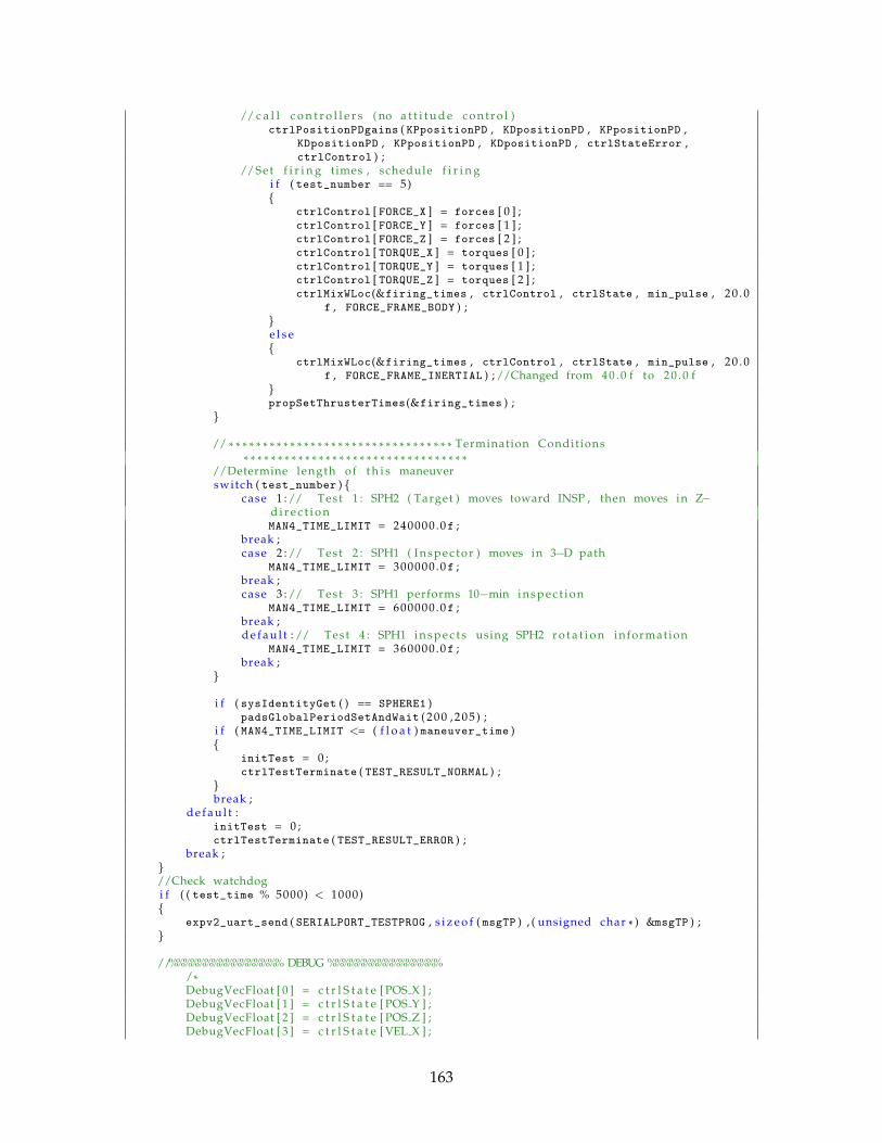
// c a l l c o n t r o l l e r s ( no a t t i t u d e c o n t r o l )ctrlPositionPDgains ( KPpositionPD , KDpositionPD , KPpositionPD ,
KDpositionPD , KPpositionPD , KDpositionPD , ctrlStateError ,ctrlControl ) ;
//Set f i r i n g times , schedule f i r i n gi f ( test_number == 5){
ctrlControl [ FORCE_X ] = forces [ 0 ] ;ctrlControl [ FORCE_Y ] = forces [ 1 ] ;ctrlControl [ FORCE_Z ] = forces [ 2 ] ;ctrlControl [ TORQUE_X ] = torques [ 0 ] ;ctrlControl [ TORQUE_Y ] = torques [ 1 ] ;ctrlControl [ TORQUE_Z ] = torques [ 2 ] ;ctrlMixWLoc(&firing_times , ctrlControl , ctrlState , min_pulse , 2 0 . 0
f , FORCE_FRAME_BODY ) ;}e l s e{
ctrlMixWLoc(&firing_times , ctrlControl , ctrlState , min_pulse , 2 0 . 0f , FORCE_FRAME_INERTIAL ) ; //Changed from 4 0 . 0 f to 2 0 . 0 f
}propSetThrusterTimes(&firing_times ) ;
}
// * * * * * * * * * * * * * * * * * * * * * * * * * * * * * * * * * Termination Conditions* * * * * * * * * * * * * * * * * * * * * * * * * * * * * * * * *
//Determine length of t h i s maneuverswitch ( test_number ) {
case 1 : // Test 1 : SPH2 ( Target ) moves toward INSP , then moves in Z−d i r e c t i o nMAN4_TIME_LIMIT = 240000 .0f ;
break ;case 2 : // Test 2 : SPH1 ( I n s p e c t o r ) moves in 3−D path
MAN4_TIME_LIMIT = 300000 .0f ;break ;case 3 : // Test 3 : SPH1 performs 10−min i n s p e c t i o n
MAN4_TIME_LIMIT = 600000 .0f ;break ;d e f a u l t : // Test 4 : SPH1 i n s p e c t s using SPH2 r o t a t i o n information
MAN4_TIME_LIMIT = 360000 .0f ;break ;
}
i f ( sysIdentityGet ( ) == SPHERE1 )padsGlobalPeriodSetAndWait ( 2 0 0 , 2 0 5 ) ;
i f ( MAN4_TIME_LIMIT <= ( f l o a t ) maneuver_time ){
initTest = 0 ;ctrlTestTerminate ( TEST_RESULT_NORMAL ) ;
}break ;
d e f a u l t :initTest = 0 ;ctrlTestTerminate ( TEST_RESULT_ERROR ) ;
break ;}//Check watchdogi f ( ( test_time % 5000) < 1000){
expv2_uart_send ( SERIALPORT_TESTPROG , s i z e o f ( msgTP ) , ( unsigned char * ) &msgTP ) ;}
//%%%%%%%%%%%%%%%% DEBUG %%%%%%%%%%%%%%%%/*DebugVecFloat [ 0 ] = c t r l S t a t e [ POS X ] ;DebugVecFloat [ 1 ] = c t r l S t a t e [ POS Y ] ;DebugVecFloat [ 2 ] = c t r l S t a t e [ POS Z ] ;DebugVecFloat [ 3 ] = c t r l S t a t e [ VEL X ] ;
163
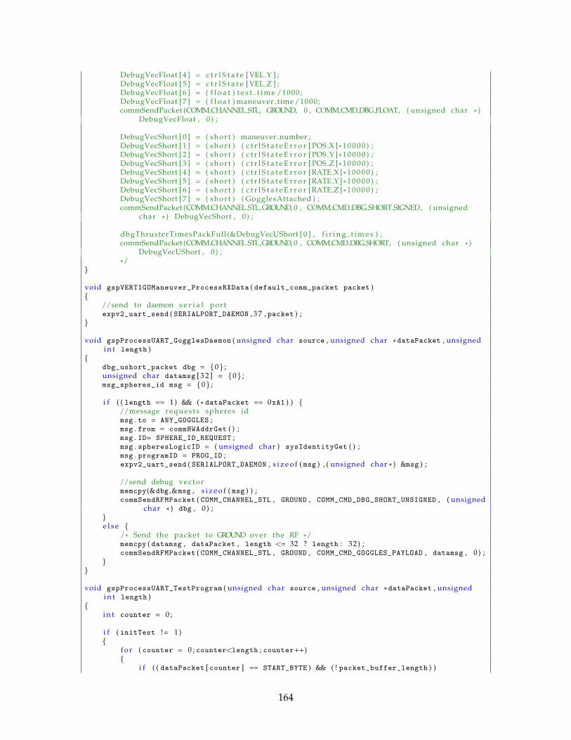
DebugVecFloat [ 4 ] = c t r l S t a t e [ VEL Y ] ;DebugVecFloat [ 5 ] = c t r l S t a t e [ VEL Z ] ;DebugVecFloat [ 6 ] = ( f l o a t ) t e s t t i m e /1000;DebugVecFloat [ 7 ] = ( f l o a t ) maneuver time /1000;commSendPacket (COMM CHANNEL STL, GROUND, 0 , COMM CMD DBG FLOAT, ( unsigned char * )
DebugVecFloat , 0 ) ;
DebugVecShort [ 0 ] = ( shor t ) maneuver number ;DebugVecShort [ 1 ] = ( shor t ) ( c t r l S t a t e E r r o r [ POS X ] * 1 0 0 0 0 ) ;DebugVecShort [ 2 ] = ( shor t ) ( c t r l S t a t e E r r o r [ POS Y ] * 1 0 0 0 0 ) ;DebugVecShort [ 3 ] = ( shor t ) ( c t r l S t a t e E r r o r [ POS Z ] * 1 0 0 0 0 ) ;DebugVecShort [ 4 ] = ( shor t ) ( c t r l S t a t e E r r o r [RATE X] * 1 0 0 0 0 ) ;DebugVecShort [ 5 ] = ( shor t ) ( c t r l S t a t e E r r o r [RATE Y] * 1 0 0 0 0 ) ;DebugVecShort [ 6 ] = ( shor t ) ( c t r l S t a t e E r r o r [RATE Z] * 1 0 0 0 0 ) ;DebugVecShort [ 7 ] = ( shor t ) ( GogglesAttached ) ;commSendPacket (COMM CHANNEL STL,GROUND, 0 , COMM CMD DBG SHORT SIGNED, ( unsigned
char * ) DebugVecShort , 0 ) ;
dbgThrusterTimesPackFull (&DebugVecUShort [ 0 ] , f i r i n g t i m e s ) ;commSendPacket (COMM CHANNEL STL,GROUND, 0 , COMM CMD DBG SHORT, ( unsigned char * )
DebugVecUShort , 0 ) ;*/
}
void gspVERTIGOManeuver_ProcessRXData ( default_comm_packet packet ){
//send to daemon s e r i a l portexpv2_uart_send ( SERIALPORT_DAEMON , 3 7 , packet ) ;
}
void gspProcessUART_GogglesDaemon ( unsigned char source , unsigned char * dataPacket , unsignedi n t length )
{dbg_ushort_packet dbg = {0} ;unsigned char datamsg [ 3 2 ] = {0} ;msg_spheres_id msg = {0} ;
i f ( ( length == 1) && ( * dataPacket == 0xA1 ) ) {//message reques t s spheres idmsg . to = ANY_GOGGLES ;msg . from = commHWAddrGet ( ) ;msg . ID= SPHERE_ID_REQUEST ;msg . spheresLogicID = ( unsigned char ) sysIdentityGet ( ) ;msg . programID = PROG_ID ;expv2_uart_send ( SERIALPORT_DAEMON , s i z e o f ( msg ) , ( unsigned char * ) &msg ) ;
//send debug vectormemcpy(&dbg ,&msg , s i z e o f ( msg ) ) ;commSendRFMPacket ( COMM_CHANNEL_STL , GROUND , COMM_CMD_DBG_SHORT_UNSIGNED , ( unsigned
char * ) dbg , 0 ) ;}e l s e {
/* Send the packet to GROUND over the RF */memcpy ( datamsg , dataPacket , length <= 32 ? length : 32 ) ;commSendRFMPacket ( COMM_CHANNEL_STL , GROUND , COMM_CMD_GOGGLES_PAYLOAD , datamsg , 0 ) ;
}}
void gspProcessUART_TestProgram ( unsigned char source , unsigned char * dataPacket , unsignedi n t length )
{i n t counter = 0 ;
i f ( initTest != 1 ){
f o r ( counter = 0 ; counter<length ; counter++){
i f ( ( dataPacket [ counter ] == START_BYTE ) && ( ! packet_buffer_length ) )
164
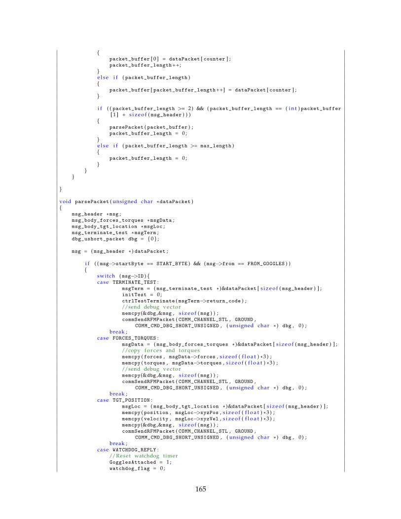
{packet_buffer [ 0 ] = dataPacket [ counter ] ;packet_buffer_length++;
}e l s e i f ( packet_buffer_length ){
packet_buffer [ packet_buffer_length++] = dataPacket [ counter ] ;}
i f ( ( packet_buffer_length >= 2) && ( packet_buffer_length == ( i n t ) packet_buffer[ 1 ] + s i z e o f ( msg_header ) ) )
{parsePacket ( packet_buffer ) ;packet_buffer_length = 0 ;
}e l s e i f ( packet_buffer_length >= max_length ){
packet_buffer_length = 0 ;}
}}
}
void parsePacket ( unsigned char * dataPacket ){
msg_header *msg ;msg_body_forces_torques * msgData ;msg_body_tgt_location * msgLoc ;msg_terminate_test * msgTerm ;dbg_ushort_packet dbg = {0} ;
msg = ( msg_header * ) dataPacket ;
i f ( ( msg−>startByte == START_BYTE ) && ( msg−>from == FROM_GOGGLES ) ){
switch ( msg−>ID ) {case TERMINATE_TEST :
msgTerm = ( msg_terminate_test * )&dataPacket [ s i z e o f ( msg_header ) ] ;initTest = 0 ;ctrlTestTerminate ( msgTerm−>return_code ) ;//send debug vectormemcpy(&dbg ,&msg , s i z e o f ( msg ) ) ;commSendRFMPacket ( COMM_CHANNEL_STL , GROUND ,
COMM_CMD_DBG_SHORT_UNSIGNED , ( unsigned char * ) dbg , 0 ) ;break ;
case FORCES_TORQUES :msgData = ( msg_body_forces_torques * )&dataPacket [ s i z e o f ( msg_header ) ] ;//copy f o r c e s and torquesmemcpy ( forces , msgData−>forces , s i z e o f ( f l o a t ) * 3 ) ;memcpy ( torques , msgData−>torques , s i z e o f ( f l o a t ) * 3 ) ;//send debug vectormemcpy(&dbg ,&msg , s i z e o f ( msg ) ) ;commSendRFMPacket ( COMM_CHANNEL_STL , GROUND ,
COMM_CMD_DBG_SHORT_UNSIGNED , ( unsigned char * ) dbg , 0 ) ;break ;
case TGT_POSITION :msgLoc = ( msg_body_tgt_location * )&dataPacket [ s i z e o f ( msg_header ) ] ;memcpy ( position , msgLoc−>xyzPos , s i z e o f ( f l o a t ) * 3 ) ;memcpy ( velocity , msgLoc−>xyzVel , s i z e o f ( f l o a t ) * 3 ) ;memcpy(&dbg ,&msg , s i z e o f ( msg ) ) ;commSendRFMPacket ( COMM_CHANNEL_STL , GROUND ,
COMM_CMD_DBG_SHORT_UNSIGNED , ( unsigned char * ) dbg , 0 ) ;break ;
case WATCHDOG_REPLY ://Reset watchdog timerGogglesAttached = 1 ;watchdog_flag = 0 ;
165
break ;}
}}
void changetoBodyFrame ( state_vector TargetState , state_vector InspectorState , f l o a t *vectorOut , unsigned i n t vectorType )
{/* T a r g e t S t a t e and I n s p e c t o r S t a t e begins in g loba l frame* . . . convert to body frame :* POS are in g loba l* VEL are in g loba l* QUAT are from globa l frame to body frame* RATE are in body* We w i l l use the quaternions to take the post ion and v e l o c i t y v e c t o r s* from the globa l frame to the body frame*/
f l o a t R_temp [ 3 ] ;f l o a t RBody [ 3 ] ;f l o a t cross [ 3 ] ;f l o a t V_temp [ 3 ] ;f l o a t mat [ 3 ] [ 3 ] ;
switch ( vectorType ) {case POSITION_VECTOR :
//Make measurements r e l a t i v e ://Moves about point a t c e n t e r of volume ( 0 , 0 , 0 )R_temp [ 0 ] = TargetState [ POS_X ] − InspectorState [ POS_X ] ;R_temp [ 1 ] = TargetState [ POS_Y ] − InspectorState [ POS_Y ] ;R_temp [ 2 ] = TargetState [ POS_Z ] − InspectorState [ POS_Z ] ;//Move to INSP Body Framequat2matrixIn ( mat , &InspectorState [ QUAT_1 ] ) ; //MAT <= r o t a t i o n matrix from globa l
to INSP bodymathMatVecMult ( RBody , ( f l o a t * * ) mat , R_temp , 3 , 3 ) ;vectorOut [ 0 ] = RBody [ 0 ] ; //POS XvectorOut [ 1 ] = RBody [ 1 ] ; //POS YvectorOut [ 2 ] = RBody [ 2 ] ; //POS Zbreak ;
case VELOCITY_VECTOR ://V = Rot * ( r ' ) − wx( Rot ( r ) ) )InspectorState [ VEL_X ] = TargetState [ VEL_X ] − InspectorState [ VEL_X ] ;InspectorState [ VEL_Y ] = TargetState [ VEL_Y ] − InspectorState [ VEL_Y ] ;InspectorState [ VEL_Z ] = TargetState [ VEL_Z ] − InspectorState [ VEL_Z ] ;mathMatVecMult ( V_temp , ( f l o a t * * ) mat , &InspectorState [ VEL_X ] , 3 , 3 ) ;mathVecCross ( cross , &InspectorState [ RATE_X ] , &InspectorState [ POS_X ] ) ;vectorOut [ 0 ] = V_temp [ 0 ] − cross [ 0 ] ; //VEL XvectorOut [ 1 ] = V_temp [ 1 ] − cross [ 1 ] ; //VEL YvectorOut [ 2 ] = V_temp [ 2 ] − cross [ 2 ] ; //VEL Zbreak ;
case ACCEL_VECTOR :vectorOut [ 0 ] = 0 . 0 f ;vectorOut [ 1 ] = 0 . 0 f ;vectorOut [ 2 ] = 0 . 0 f ;break ;
case ROTATION_VECTOR ://Move TGT Rot in TGT Body to INSP BodyR_temp [ 0 ] = TargetState [ RATE_X ] ; //Get TGT Rotat ion Rates in TGT Body FrameR_temp [ 1 ] = TargetState [ RATE_Y ] ;R_temp [ 2 ] = TargetState [ RATE_Z ] ;quat2matrixOut ( mat , &TargetState [ QUAT_1 ] ) ; //MAT <= r o t a t i o n matrix from TGT Body
to GlobalmathMatVecMult ( RBody , ( f l o a t * * ) mat , R_temp , 3 , 3 ) ; //TGT Body to GlobalR_temp [ 0 ] = RBody [ 0 ] ;R_temp [ 1 ] = RBody [ 1 ] ;R_temp [ 2 ] = RBody [ 2 ] ;
166
memset ( RBody , 0 , s i z e o f ( f l o a t ) * 3 ) ;quat2matrixIn ( mat , &InspectorState [ QUAT_1 ] ) ; //MAT <= r o t a t i o n matrix from globa l
to INSP bodymathMatVecMult ( RBody , ( f l o a t * * ) mat , R_temp , 3 , 3 ) ; //Global to INSP Body//vectorOut = ROT RATE DIR[0−2]vectorOut [ 0 ] = RBody [ 0 ] ; //XvectorOut [ 1 ] = RBody [ 1 ] ; //YvectorOut [ 2 ] = RBody [ 2 ] ; //Z//Find Magnitude//ROT RATE TGTvectorOut [ 3 ] = ( f l o a t ) sqrt ( vectorOut [ 0 ] * vectorOut [ 0 ] + vectorOut [ 1 ] * vectorOut [ 1 ] +
vectorOut [ 2 ] * vectorOut [ 2 ] ) ;break ;
d e f a u l t :initTest = 0 ;ctrlTestTerminate ( 1 3 ) ; //ERROR: I n c o r r e c t c a l l to changetoBodyFramebreak ;
}}
167

THIS PAGE INTENTIONALLY LEFT BLANK
168

Appendix B
VERTIGO System Requirements
169

The VERTIGO Project
VERTIGO is a DARPA-funded project which combines the knowledge of the MIT Space Systems
Laboratory with the flight hardware experience of Aurora Flight Sciences in a partnership to upgrade the
current SPHERES testbed on the International Space Station. Launched in 2006, SPHERES is a 6-degree of
freedom control and navigation testbed which has proved invaluable to scientists and engineers seeking
to test algorithms in a microgravity environment. VERTIGO seeks to add visual navigation to the
capabilities of SPHERES by adding a set of “Goggles” which combine a pair of cameras for stereo vision
with processing and communications hardware upgrades. Individually, these two items are called the
camera and avionics stack.
Primary Mission Objectives
The Primary Mission Objective of the VERTIGO Program is to upgrade the SPHERES satellites to enable
the rapid and flexible research and development (R&D) of Vision-Based Navigation (VBN) Algorithms in a
“shirt-sleeve micro-gravity environment” inside the International Space Station. Specifically, VERTIGO
will allow one or two SPHERES satellites to construct a 3D model of an unknown object (possibly moving
and tumbling) without any a priori state knowledge. Two inspector SPHERES satellites will perform
relative navigation solely by sensory reference to the target object. The performance of this algorithm
will be verified using the SPHERES Global Metrology System and a CAD model of the target object.
[PMO]
This can be summarized as follows:
1. Develop an algorithm to construct a 3D map of an object and use the map for relative
navigation. [MO 1]
2. Rapid Research and Development of Vision-Based Navigation. [MO 2]
3. Flexible Research and Development of Vision-Based Navigation. [MO 3]
Definitions
1. “Rapid” – in the context of R&D for VBN, rapid implies that algorithms should be able to be
developed by a small research team working during an academic year with results obtained
within an academic semester.
2. “Flexible” – The VERTIGO System must allow different types of vision-based navigation
algorithms to test the relative advantages and disadvantages of each approach.
3. The VERTIGO System (the System): comprises the SPHERES satellite(s), attached Goggles, the
Flight GUI on the Space Station/Express Rack Computer (SSC/ERC), and support equipment.
4. SPHERESCore Software: that software which exists within the SPHERES Satellites, independent
of any peripheral hardware.
5. The Flight GUI: the software onboard the SSC/ERC which allows astronauts onboard the ISS to
interact with the SPHERES testbed and related hardware.
6. The Goggles Onboard Software: the software which is loaded onto the Goggles and exists
independent of the SPHERE that the Goggles are attached to.

Reference Documents
Reference documents will be used in their current state as of 12 April 2011.
1. SSP 57000, Pressurized Payloads Interface Requirements Document, International Space Station
Program
2. SSP 50313, Display and Graphics Commonality Standard (DGCS)
3. SSP 50835, ISS Pressurized Volume Hardware, Common Interface Requirements Document
4. SSP 51700, Payload Safety Policy and Requirements for the International Space Station
5. JSC 20793, Crewed Space Vehicle Battery Safety Requirements
System Requirements
1. The VERTIGO System must use cameras to estimate the structure of an object with no a priori
knowledge of that object. [SR 10]
Rationale: this derives from Mission Objective (MO) 1.
2. The VERTIGO System must use cameras to estimate the angular and translational velocities of
the inspected object. [SR 20]
Rationale: this derives from MO 1.
3. Two inspector SPHERES must navigate around the inspected object using its estimated structure
and velocities. [SR 30]
Rationale: this derives from MO 1.
4. The System must be able to upload and run new tests and download data from tests. [SR 40]
Rationale: this derives from MO 3.
5. The VERTIGO Goggles must attach to the existing SPHERES Satellites and be compatible with the
SPHERES Flight GUI. [SR 50]
Rationale: this derives from the Primary Mission Objectives (PMO) and MO 2.
6. The VERTIGO System must be operated by astronauts inside the International Space Station. [SR
60].
Rationale: this derives from the PMO.

Functional Requirements
1. The VERTIGO System must use cameras to estimate in 3 dimensions the structure of an object
with no a priori knowledge of that object.
a. An observing SPHERES satellite must use only onboard cameras, accelerometers,
gyroscopes, and knowledge of its own dynamics in constructing the estimated structure.
[FR 10]
Rationale: These restrictions are from the PMO.
b. The algorithm must use one or two SPHERES satellites in the development of the 3D
model. [FR 20]
Rationale: this requirement flows directly from the PMO.
c. The System must sense depth and light intensity of scenes including the target object.
[FR 30]
d. The System must process the sensor information to obtain depth and light information.
[FR 40]
e. The System must store the 3D structure representation of the inspected object. [FR 50]
2. The VERTIGO System must use cameras to estimate the angular and translational velocities of
the inspected object.
a. The System must be able to identify features. [FR 60]
b. The System must be capable of tracking features on the object at TBD ms intervals as
the object moves at no more than TBD radians per second and TBD meters per second.
[FR 70].
c. The system must store estimated angular and translational velocities of the inspected
object. [FR 80]
3. Two inspector SPHERES must navigate around the inspected object using the knowledge of its
structure and velocities.
a. The 3D model must be accurate enough to safely navigate around another satellite
(TPM 01: 5cm). [FR 90]
b. Inspecting SPHERES satellites must be able to share real-time video between their
attached Goggles with no loss of pixel information. [FR 100]
Rationale: in order to develop a map jointly, known vision-based navigation
algorithms require this information to be shared between the two inspectors.
c. The VERTIGO Team must supply at least two (2) SPHERES Goggles for launch to the
International Space Station. [FR 110]
Rationale: the requirement to use 2 SPHERES as inspectors implies a need for at
least 2 Goggles to be launched.
4. The System must be able to upload and run new tests and download data from tests.
a. The VERTIGO System must provide methods for new algorithms to be programmed. [FR
120]
Rationale: this is to support the flexibility MO.
b. THE VERTIGO System must provide a method for new programs to be uploaded to the
ISS compatible with the existing SPHERES upload procedures. [FR 130]
c. The VERTIGO System aboard the ISS must be able to load the new programs in a method
compatible with the existing SPHERES loading procedures. [FR 140]
d. Data must be stored onboard the VERTIGO System until it can be downloaded to
Ground. [FR 150]
e. Data must be stored in files that can be downloaded using existing ISS wireless
communications infrastructure. [FR 160]
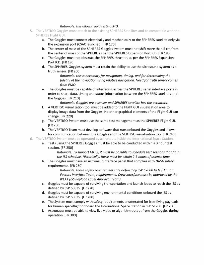
Rationale: this allows rapid testing MO.
5. The VERTIGO Goggles must attach to the existing SPHERES Satellites and be compatible with the
SPHERES Flight GUI.
a. The Goggles must connect electrically and mechanically to the SPHERES satellite only via
the expansion port (CSAC launched). [FR 170]
b. The center of mass of the SPHERES-Goggles system must not shift more than 5 cm from
the center of mass of the SPHERE as per the SPHERES Expansion Port ICD. [FR 180]
c. The Goggles must not obstruct the SPHERES thrusters as per the SPHERES Expansion
Port ICD. [FR 190]
d. The SPHERES-Goggles system must retain the ability to use the ultrasound system as a
truth sensor. [FR 200]
Rationale: this is necessary for navigation, timing, and for determining the
fidelity of the navigation using relative navigation. Need for truth sensor comes
from PMO.
e. The Goggles must be capable of interfacing across the SPHERES serial interface ports in
order to share data, timing and status information between the SPHERES satellites and
the Goggles. [FR 210]
Rationale: Goggles are a sensor and SPHERES satellite has the actuators.
f. A VERTIGO visualization tool must be added to the Flight GUI visualization area to
display image data from the Goggles. No other graphical elements of the Flight GUI can
change. [FR 220]
g. The VERTIGO System must use the same test management as the SPHERES Flight GUI.
[FR 230]
h. The VERTIGO Team must develop software that runs onboard the Goggles and allows
for communication between the Goggles and the VERTIGO visualization tool. [FR 240]
6. The VERTIGO System must be operated by astronauts inside the International Space Station.
a. Tests using the SPHERES Goggles must be able to be conducted within a 3 hour test
session. [FR 250]
Rationale: To support MO 2, it must be possible to schedule test sessions that fit in
the ISS schedule. Historically, these must be within 2-3 hours of science time.
b. The Goggles must have an Astronaut interface panel that complies with NASA safety
requirements. [FR 260]
Rationale: these safety requirements are defined by SSP 57000 HFIT (Human
Factors Interface Team) requirements. Crew interface must be approved by the
IPLAT (ISS Payload Label Approval Team).
c. Goggles must be capable of surviving transportation and launch loads to reach the ISS as
defined by SSP 50835. [FR 270]
d. Goggles must be capable of surviving environmental conditions onboard the ISS as
defined by SSP 50835. [FR 280]
e. The System must comply with safety requirements enumerated for free-flying payloads
for human spaceflight onboard the International Space Station in SSP 51700. [FR 290]
f. Astronauts must be able to view live video or algorithm output from the Goggles during
operation. [FR 300]
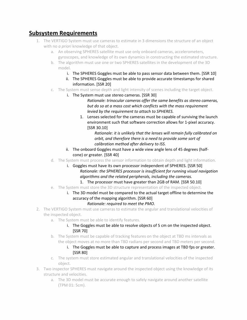
Subsystem Requirements
1. The VERTIGO System must use cameras to estimate in 3 dimensions the structure of an object
with no a priori knowledge of that object.
a. An observing SPHERES satellite must use only onboard cameras, accelerometers,
gyroscopes, and knowledge of its own dynamics in constructing the estimated structure.
b. The algorithm must use one or two SPHERES satellites in the development of the 3D
model.
i. The SPHERES Goggles must be able to pass sensor data between them. [SSR 10]
ii. The SPHERES Goggles must be able to provide accurate timestamps for shared
information. [SSR 20]
c. The System must sense depth and light intensity of scenes including the target object.
i. The System must use stereo cameras. [SSR 30]
Rationale: trinocular cameras offer the same benefits as stereo cameras,
but do so at a mass cost which conflicts with the mass requirement
levied by the requirement to attach to SPHERES.
1. Lenses selected for the cameras must be capable of surviving the launch
environment such that software correction allows for 1-pixel accuracy.
[SSR 30.10]
Rationale: it is unlikely that the lenses will remain fully calibrated on
orbit, and therefore there is a need to provide some sort of
calibration method after delivery to ISS.
ii. The onboard Goggles must have a wide view angle lens of 45 degrees (half-
cone) or greater. [SSR 40]
d. The System must process the sensor information to obtain depth and light information.
i. Goggles must have its own processor independent of SPHERES. [SSR 50]
Rationale: the SPHERES processor is insufficient for running visual navigation
algorithms and the related peripherals, including the cameras.
1. The processor must have greater than 2GB of RAM. [SSR 50.10]
e. The System must store the 3D structure representation of the inspected object.
i. The 3D model must be compared to the actual target offline to determine the
accuracy of the mapping algorithm. [SSR 60]
Rationale: required to meet the PMO.
2. The VERTIGO System must use cameras to estimate the angular and translational velocities of
the inspected object.
a. The System must be able to identify features.
i. The Goggles must be able to resolve objects of 5 cm on the inspected object.
[SSR 70]
b. The System must be capable of tracking features on the object at TBD ms intervals as
the object moves at no more than TBD radians per second and TBD meters per second.
i. The Goggles must be able to capture and process images at TBD fps or greater.
[SSR 80]
c. The system must store estimated angular and translational velocities of the inspected
object.
3. Two inspector SPHERES must navigate around the inspected object using the knowledge of its
structure and velocities.
a. The 3D model must be accurate enough to safely navigate around another satellite
(TPM 01: 5cm).

i. The estimated trajectory must be compared to the ultrasonic time-of-flight
“ground truth” provided by the global metrology system. [SSR 90]
ii. Cameras must be able to track 5 cm point features in the image and compute
stereo disparity in ISS interior lighting conditions for motion of less than 5 cm/s
and 6 deg/s at distances between 50 cm and 3 m. [SSR 100]
Rationale: Numbers are based on a 1 meter diameter circle in 60 seconds.
Lighting conditions are defined in reference documents (SSPs).
1. Cameras must have a minimum of 640x480 resolution for use in the
developed algorithms. [SSR 100.10]
2. If optical testing of the algorithms show it to be necessary, the Goggles
must include an illuminating LED light which meets SSP 51700 and SSP
57000, with the appropriate power regulators. [SSR 100.20]
b. Inspecting SPHERES satellites must be able to share real-time video between their
attached Goggles with no loss of pixel information.
i. The data transfer method between inspector SPHERES must operate with a
latency of TBD ms or less. [SSR 110]
ii. A wireless data link of at least 70 Mbps within the test volume must be available
between the two inspector SPHERES. [SSR 130]
Rationale: a minimum link of 35 Mbps (bidirectionally) is needed to share
the expected amount of real-time video coming from the Goggles. This is
derived from 10fps, 640x480 8-bit grayscale images that are losslessly
compressed. Wireless is necessary because wires running to a SPHERE would
severely inhibit its ability to build a 3D map and maneuver around the test
volume.
1. The Goggles must use 802.11n or similar architectures to communicate.
[SSR 130.10]
Rationale: 802.11n is the only currently available 802.11
standard which allows for bi-directional rates at or above 70
Mbps.
c. The VERTIGO Team must supply at least two (2) SPHERES Goggles for launch to the
International Space Station.
4. The System must be able to upload and run new tests and download data from tests.
a. The VERTIGO System must provide methods for new algorithms to be programmed.
b. THE VERTIGO System must provide a method for new programs to be uploaded to the
ISS compatible with the existing SPHERES upload procedures.
i. There must be a method for libraries installed on the Goggles to be updated
while on station. [SSR 140]
Rationale: to meet MO 3 while satisfying MO 2, as new open source
libraries become available, updating those on the ISS should be possible.
ii. The Goggles disk image must be able to be completely replaced. [SSR 150]
1. The disk image must be able to be connected directly to the SSC/ERC.
[SSR 150.10]
2. The Flight GUI must provide a mechanism for reimaging a disk that is
connected to the SSC/ERC. [SSR 150.20]
c. The VERTIGO System aboard the ISS must be able to load the new programs in a method
compatible with the existing SPHERES loading procedures.
i. The VERTIGO Goggles must have a method of receiving new programs from the
SSC/ERC. [SSR 160]

d. Data must be stored onboard the VERTIGO System until it can be downloaded to
Ground.
i. Goggles must have a hard disk (HD) of at least 16GB. [SSR 170]
Rationale: During a test session, at least 13GB of data is expected to be
generated. This is computed based on four (4) 640x480 8-bit images at
10 fps for 20 minutes.
e. Data must be stored in files that can be downloaded using existing ISS wireless
communications infrastructure.
i. Data from SPHERES must reside in an acceptable file format as per Ground Rules
& Constraints document. [SSR 180]
ii. Files must be of an acceptable file size as per Ground Rules & Constraints
document. [SSR 190]
5. The VERTIGO Goggles must attach to the existing SPHERES.
a. The Goggles must connect electrically and mechanically to the SPHERES satellite only via
the expansion port (CSAC launched).
i. Goggles power must be provided by the Goggles system. [SSR 200]
Rationale: the power that can be supplied through the expansion port is
insufficient for the Goggles processing needs.
b. The center of mass of the SPHERES-Goggles system must not shift more than 5 cm from
the center of mass of the SPHERE as per the SPHERES Expansion Port ICD.
i. SPHERES Goggles hardware must have a mass less than 1.5 kg. [SSR 210]
Rationale: based on the dry mass distribution, a mass of more than 1.5
kg will shift the center of mass beyond the 5 cm limit enumerated above.
c. SPHERES thrusters must be unobstructed by the Goggles as per the SPHERES Expansion
Port ICD.
i. The Goggles must remain outside of a TBD volume around the SPHERES
Thrusters. [SSR 220]
ii. Communication within the VERTIGO System must be wireless. [SSR 230]
Rationale: wires connected to the satellites will impede control. Need
this requirement to support rapid MO.
d. The SPHERES-Goggles system must retain the ability to use the ultrasound system as a
truth sensor.
i. The Goggles must remain outside of a TBD volume around SPHERES ultrasonic
microphones as per the SPHERES Expansion Port ICD. [SSR 240]
ii. The Goggles must remain outside of a TBD volume around the SPHERES IR
beacon as per the SPHERES Expansion Port ICD. [SSR 250]
e. The Goggles must be capable of interfacing across the SPHERES serial interface ports in
order to share data, timing and status information between the SPHERES satellites and
the Goggles.
i. Attached Goggles must be capable of accepting IMU data transmitted from
SPHERES at a rate of at least 20 Hz and with a timestamp that is accurate to at
least TBD ms. [SSR 260]
Rationale: these standards are already able to be met by SPHERES,
acting in concert with the ultrasonic global metrology system. Delays
greater than TBD ms are expected to impact the fusion of the IMU and
vision data.
ii. IMU data must have a latency of no more than 5 ms or no more than 2 ms
latency added on top of transmission time. [SSR 270]
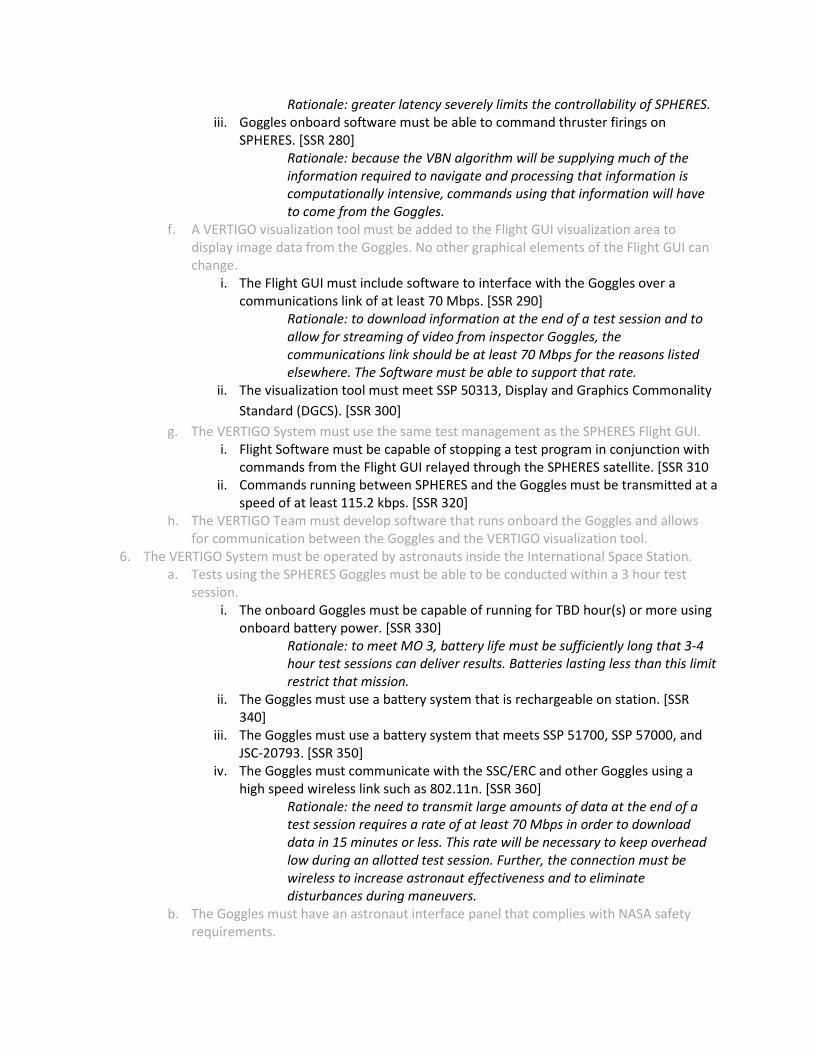
Rationale: greater latency severely limits the controllability of SPHERES.
iii. Goggles onboard software must be able to command thruster firings on
SPHERES. [SSR 280]
Rationale: because the VBN algorithm will be supplying much of the
information required to navigate and processing that information is
computationally intensive, commands using that information will have
to come from the Goggles.
f. A VERTIGO visualization tool must be added to the Flight GUI visualization area to
display image data from the Goggles. No other graphical elements of the Flight GUI can
change.
i. The Flight GUI must include software to interface with the Goggles over a
communications link of at least 70 Mbps. [SSR 290]
Rationale: to download information at the end of a test session and to
allow for streaming of video from inspector Goggles, the
communications link should be at least 70 Mbps for the reasons listed
elsewhere. The Software must be able to support that rate.
ii. The visualization tool must meet SSP 50313, Display and Graphics Commonality
Standard (DGCS). [SSR 300]
g. The VERTIGO System must use the same test management as the SPHERES Flight GUI.
i. Flight Software must be capable of stopping a test program in conjunction with
commands from the Flight GUI relayed through the SPHERES satellite. [SSR 310
ii. Commands running between SPHERES and the Goggles must be transmitted at a
speed of at least 115.2 kbps. [SSR 320]
h. The VERTIGO Team must develop software that runs onboard the Goggles and allows
for communication between the Goggles and the VERTIGO visualization tool.
6. The VERTIGO System must be operated by astronauts inside the International Space Station.
a. Tests using the SPHERES Goggles must be able to be conducted within a 3 hour test
session.
i. The onboard Goggles must be capable of running for TBD hour(s) or more using
onboard battery power. [SSR 330]
Rationale: to meet MO 3, battery life must be sufficiently long that 3-4
hour test sessions can deliver results. Batteries lasting less than this limit
restrict that mission.
ii. The Goggles must use a battery system that is rechargeable on station. [SSR
340]
iii. The Goggles must use a battery system that meets SSP 51700, SSP 57000, and
JSC-20793. [SSR 350]
iv. The Goggles must communicate with the SSC/ERC and other Goggles using a
high speed wireless link such as 802.11n. [SSR 360]
Rationale: the need to transmit large amounts of data at the end of a
test session requires a rate of at least 70 Mbps in order to download
data in 15 minutes or less. This rate will be necessary to keep overhead
low during an allotted test session. Further, the connection must be
wireless to increase astronaut effectiveness and to eliminate
disturbances during maneuvers.
b. The Goggles must have an astronaut interface panel that complies with NASA safety
requirements.
i. The astronaut interface panel must have an on/off switch. [SSR 370]
ii. The astronaut interface panel must have a reset button. [SSR 380]
c. Goggles must be capable of surviving transportation and launch loads to reach the ISS as
defined by SSP 50835.
d. Goggles must be capable of surviving environmental conditions onboard the ISS as
defined by SSP 50835.
e. The System must comply with safety requirements enumerated for free-flying payloads
for human spaceflight onboard the International Space Station in SSP 51700.
f. Astronauts must be able to view live video or algorithm output from the Goggles during
operation.
i. The Goggles onboard software must provide a low resolution/low bandwidth
video display of the Goggles Algorithms for the astronauts to monitor using the
VERTIGO visualization tool. [SSR 390]
Rationale: video output from the Goggles allows algorithm performance
feedback from astronauts.
Bibliography
[1] R. R. Britt. Is Hubble Worth the Upgrade Mission’s Risk and Cost? http://www.
livescience.com/3579-hubble-worth-upgrade-mission-risk-cost.html, 2011.[online periodical].
[2] D. Leone. NASA: James Webb Telescope Expected to Cost $8.7 Billion. http://
spacenews.com/civil/110826-jwst-cost-billion.html, 2009. [online periodical].
[3] A. E. Turner. Cost-Effective Spacecraft Dependent Upon Frequent Non-Intrusive Ser-vicing. AIAA, August 28-30 2001.
[4] Broad Agency Announcement: Phoenix Technologies. DARPA-BAA-12-02, 2011.DARPA-BAA-12-02.
[5] J. L. Ruiz and C. H. Frey. Geosynchronous Satellite Use of GPS. pages 1227–1232,2005.
[6] Global Positioning System Standard Positioning Service Performance Standard, 2008.
[7] I. Nygren and M. Jansson. Terrain navigation for underwater vehicles using the cor-relator method. Oceanic Engineering, IEEE Journal of, 29(3):906 – 915, july 2004.
[8] K Machida. Space test of sensor-fused telerobotics for high-precision tasks. Journal ofSpacecraft and Rockets, 41(1):132–139, 2004.
[9] Deborah Meduna. Terrain relative navigation for sensor-limited systems with applicationto underwater vehicles. Phd, Stanford University, 08/2011 2011.
[10] J. P. Curran D. S. Moyer R. L. Strachan I. Mills D. P. Goodwin, L. E. Hembree and J.-S.Valois. Orbiter space vision system on space shuttle flight sts-80. SPIE, 3074:18–28,1997.
[11] R.T. Howard, A.F. Heaton, R.M. Pinson, and C.K. Carrington. Orbital Express Ad-vanced Video Guidance Sensor. In Aerospace Conference, 2008 IEEE, pages 1 –10, march2008.
[12] Daniel Sheinfeld and Stephen M. Rock. Rigid Body Inertia Estimation with Applica-tions to the Capture of a Tumbling Satellite. February 2009.
[13] Peter Kimball. Iceberg-Relative Navigation for Autonomous Underwater Vehicles. Phd,Stanford University, Stanford, CA, 08/2011 2011.
179
[14] Peter Kimball and Stephen M. Rock. Sonar-based iceberg-relative navigation for au-tonomous underwater vehicles. Deep Sea Research Part II: Topical Studies in Oceanogra-phy, 58(11-12):1301 – 1310, 2011. Free-Drifting Icebergs in the Southern Ocean.
[15] Kiran Murthy and Stephen M. Rock. Navigation for Performing Visual Surveys ofNon-Planar Surfaces. In Proceedings of AIAA Guidance, Navigation, and Control Confer-ence, 2009.
[16] Kiran Murthy and Stephen M. Rock. Spline-based Trajectory Planning Techniquesfor Benthic AUV Operations. In Proceedings of IEEE Autonomous Underwater VehiclesConference, 2010.
[17] O. Yakimenko G. Boyarko and M. Romano. Optimal Rendezvous Trajectories of aControlled Spacecraft and a Tumbling Object. AIAA Journal of Guidance, Control, andDynamics, 34(4):1239–1252, July-August 2011.
[18] J. L. Crassidis R. Linares and Y. Cheng. Constrained Relative Attitude Determina-tion for Two-Vehicle Formations. AIAA Journal of Guidance, Control, and Dynamics,34(2):543–553, March-April 2011.
[19] H. B. Hablani. Autonomous Inertial Relative Navigation with Sight-Line-StabilizedIntegrated Sensors for Spacecraft Rendezvous. AIAA Journal of Guidance, Control, andDynamics, 32(1):172–183, January-February 2009.
[20] A. Weichbrod J. DiMatteo, D. Florakis and M. Milam. Proximity Operations Testingwith a Rotating and Translating Resident Space Object. August 10-13 2009.
[21] Kiran Murthy. A Trajectory Optimization Method for Close Range Surveys of Non-Planar Surfaces. Master’s thesis, Stanford University, 03/2012 2012.
[22] B. K. P. Horn. Robot Vision. MIT Press, 1998.
[23] David G. Lowe. Distinctive Image Features from Scale-Invariant Keypoints. Int. J.Comput. Vision, 60(2):91–110, November 2004.
[24] Allen Chen. Propulsion System Characterization for the SPHERES Formation Flightand Docking Testbed. Master’s thesis, Massachusetts Institute of Technology, May2002. S.M. Thesis.
[25] Reaction Control System. http://science.ksc.nasa.gov/shuttle/technology/
sts-newsref/sts-rcs.html, 1988/2000.
[26] V. Zalgaller. Shortest Inspection Curves for the Sphere. Journal of Mathematical Sciences,131:5307–5320, 2005. 10.1007/s10958-005-0403-9.
[27] Paul Bourke. Baseball seam curve. http://paulbourke.net/geometry/baseball/,January 2001.
[28] Simon Nolet. Development of a Guidance, Navigation and Control Architecture and Val-idation Process Enabling Autonomous Docking to a Tumbling Satellite. Scd, Departmentof Aeronautics and Astronautics, Massachusetts Institute of Technology, Cambridge,MA, 2007.
180
[29] Simon Nolet. The SPHERES Navigation System: from Early Development to On-Orbit Testing. AIAA Guidance, Navigation and Control Conference and Exhibit, August20-23 2007.
[30] Brent E Tweddle, Alvar Saenz-Otero, and David W Miller. Design and Developmentof a Visual Navigation Testbed for Spacecraft Proximity Operations. In AIAA SPACE2009 Conference Exposition, number September. American Institute of Aeronautics andAstronautics, 2009.
[31] Bill Triggs, Philip McLauchlan, Richard Hartley, and Andrew Fitzgibbon. BundleAdjustment — A Modern Synthesis. In Bill Triggs, Andrew Zisserman, and RichardSzeliski, editors, Vision Algorithms: Theory and Practice, volume 1883 of Lecture Notes inComputer Science, pages 153–177. Springer Berlin / Heidelberg, 2000.
[32] R. Smith, M. Self, and P. Cheeseman. Autonomous robot vehicles. chapter Estimatinguncertain spatial relationships in robotics, pages 167–193. Springer-Verlag New York,Inc., New York, NY, USA, 1990.
[33] Brent Tweddle. Relative Computer Vision Based Navigation for Small InspectionSpacecraft. Aug 8-11 2011.
[34] Brent Tweddle. Computer Vision Based Navigation for Spacecraft Proximity Opera-tions. Master’s thesis, Department of Aeronautics and Astronautics, MassachusettsInstitute of Technology, 2010. S.M. Thesis.
[35] Oliver J. Woodman. An introduction to inertial navigation. Technical Report 696,University of Cambridge Computer Laboratory, 15 JJ Thomson Avenue, CambridgeCB3 0FD, United Kingdom, August 2007.
[36] SPHERES Fact Sheet, May 20 2007.
181