Design and Implementation of a Low Complexity Multiuser

Design and Implementation of a Low ComplexityMultiuser Detector for Hybrid CDMA Systems

Vittorio Rampa

Abstract— In hybrid CDMA systems, multiuser detection(MUD) algorithms are adopted at the base station to reduceboth multiple access and inter-symbol interference by exploitingspace-time (ST) signal processing techniques. Linear ST-MUDalgorithms solve a linear problem where the system matrixhas a block-Toeplitz shape. While exact inversion techniquesimpose an intolerable computational load, reduced complexityalgorithms may be efficiently employed even if they show sub-optimal behavior introducing performance degradation and near-far effects. The block-Fourier MUD algorithm is generallyconsidered the most effective one. However, the block-BareissMUD algorithm, that has been recently reintroduced, shows alsogood performance and low computational complexity comparingfavorably with the block-Fourier one. In this paper, both MUDalgorithms will be compared, along with other well knownones, in terms of complexity, performance figures, hardwarefeasibility and implementation issues. Finally a short hardwaredescription of the block-Bareiss and block-Fourier algorithmswill be presented along with the FPGA (Field ProgrammableGate Array) implementation of the block-Fourier using standardVHDL (VHSIC Hardware Description Language) design.

Index Terms— Low complexity multiuser detector, hybridCDMA system, TD-SCDMA mobile radio system, CWTS, block-Bareiss algorithm, block-Fourier algorithm, FPGA implementa-tion.

I. INTRODUCTION

In 3G hybrid CDMA systems with antenna arrays at thereceivers, space-time (S-T) multiuser detection (MUD) algo-rithms are adopted at the base station to reduce both inter-symbol (ISI) and multiple access (MAI) interference [1]. Foreach data-packet or block, in the up-link scenario, linear MUDsolves a linear system where the system matrix has a specificblock-Toeplitz structure.

Exact MUD computation exhibits a high computational loadfor large matrix size (i.e. high number of users, antennas and/orsymbols per block), as it involves the inversion of a largecorrelation matrix. Exact inversion of the system matrix isnot feasible due to large matrix size and real-time constraints.In fact, in real-time mobile radio systems, computationalresources are limited and only reduced complexity algorithmscan be employed. Nevertheless, when computational complex-ity is strongly reduced, sub-optimal algorithms might introduce

Manuscript received September 04, 2004; revised May 09, 2005 and August31, 2005. The paper was presented in part at the Conference on Software,Telecommunications and Computer Networks (SoftCOM) 2004.

Author is with IEIIT - Sezione di Milano – CNR, Via Ponzio 34/5, Milano,20133 (MI), Italy (e-mail: [email protected]).Digital Object Identifier: 01.5010/JCOMSS.2005.010109

performance degradation and other unwanted effects (e.g. near-far problems).

Two main MUD techniques are available in literature: block-based MUD [2],[3],[4] and one-shot MUD also known assliding windows detector (SWD) [5]. Both families may beimplemented using real-time hardware [4],[6],[7],[8],[9],[10].In practice, algorithm selection is performed taking into ac-count various aspects such as performance, complexity andimplementation issues. However, when computational powerrequirement and system complexity are the key constraints,some performance degradation have to be tolerated.

According to these considerations, a new MUD detectorscheme based on the block-Bareiss (BB) algorithm has beenreintroduced [11],[12]. This algorithm, derived from the plainBareiss factorization technique [13], combines good perfor-mance and low computational load with simple hardwareimplementation. For a specific hybrid CDMA radio system(i.e. China Wireless Telecommunication Standard or CWTS forshort), the BB detector is compared with the reference directinversion methods and with other well known block algorithmsnamely the block-Levinson algorithm (BL) [14] and the block-Fourier Transform (BFT) algorithm [4].

Finally a floating-point implementation of the BB processoris compared with the equivalent BFT one. With respect to theabove mentioned algorithms, the BB one is well suited forhardware FPGA (Field Programmable Gate Array) implemen-tation not only for its low computational load but also for itsgood performance. In addition, it does not suffer from near-far effects that plague very low complexity implementationsuch as low order BFT detectors [15]. It is also worth noticingthat the BB detector is also suitable for hardware parallelimplementation. However, for perfect power control radiosystems, the BFT remains the most effective MUD algorithmin terms of complexity and implementation feasibility. Finally,a FPGA implementation of the BFT algorithm is presentedand commented.

The paper is organized as follows: Section II describes thesignal model used in hybrid CDMA systems and underlinesthe peculiarities due to the specific CWTS standard adopted.Section III introduces the Bareiss algorithm and the otherreduced complexity algorithms selected for comparison. Bothperformance and computational complexity of the mentionedMUD algorithms are evaluated and compared in Sections IVand V, respectively. The proposed hardware implementationis described in Section VI while Section VII draws someconclusions.

42 JOURNAL OF COMMUNICATIONS SOFTWARE AND SYSTEMS, VOL. 1, NO. 1, SEPTEMBER 2005

1845-6421/05/5010 © 2005 CCIS

user

Rectangle

FESB

Typewritten Text

Original scientific paper

Radio frameSubframe 0

10 ms

5 ms675 µs

TS3 TS4 TS5 TS6TS2TS1UpPTSGPDwPTSTS0

75 µs 125 µs75 µs

Midamble(144 chips)

GP(16 chips)

Data symbols(352 chips)

Subframe

Time slot

275 µs 275 µs112.5 µs 12.5 µs



Subframe 0

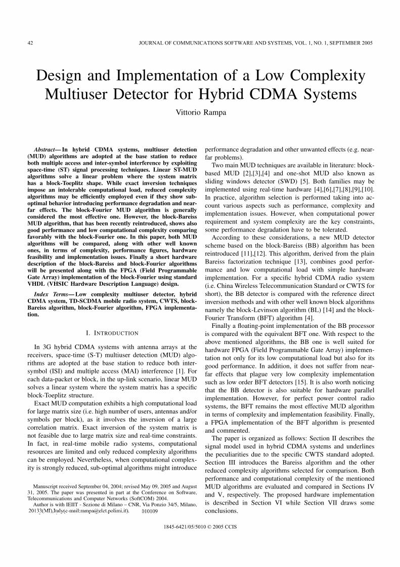
Fig. 1. Up-link burst structure for the CWTS system.

II. HYBRID CDMA SIGNAL MODEL

In hybrid synchronous CDMA systems, such as the CWTSstandard [16] whose frame structure is shown in Fig. 1, Kusers (1 ≤ K ≤ 8) are active in the same frequency bandand in the same time slot being separated only by differentspreading codes. Each user transmits a data burst consisting of2N QPSK symbols (N = 352/Q, N symbols of duration Ts =QTc) where Q is the spreading factor (Q ∈ {1, 2, 4, 8, 16})and the chip rate Fc is defined as Fc = 1/Tc = 1.28 Mcps.In the following part of this paper, Q is assumed constant forall K users: Q = 16. The semi-burst period Tsb is defined asTsb = NQTc = 352/Fc = 275 µs.

The column vector hk,m represents the channel impulseresponse (CIR) for the link between the kth user and the mthantenna of the array. Each vector hk,m is also assumed oflength W (W = 16) when expressed in chip intervals TC .Space-time matrix Hk = [hk,1...hk,m...hk,M ]T for the kthuser has size M × W while the complete multi-user channelmatrix H = [H1...HK ] has size M × WK. Each CIR isassumed known and does not vary during the time slot.

For each semi-burst, the discrete-time base-band MIMO(Multiple Input Multiple Output) signal model is indicated bythe following equation:

y = Ad + n. (1)

The M(NQ + W − 1) × 1 vector y represents the signalreceived by the array of M antennas (1 ≤ M ≤ 8) located atthe base station while vector d of size NK × 1 represents thetransmitted data for all K users. Moreover, it is E

[ddH

]= I.

Noise vector n takes care of both electronic noise and inter-cellinterference; n is assumed spatially correlated and temporallyuncorrelated with covariance matrix given by:

Rn = E[nnH] = Rn ⊗ INQ+W−1, (2)

where ⊗ is the Kronecker’s product, INQ+W−1 is the identitymatrix of size NQ + W − 1 and Rn is the spatial covariancematrix ([Rn]m,m = σ2

n for m = 1, ...,M ) of size M ×M .Since the CIRs are assumed constant in the data slot, the

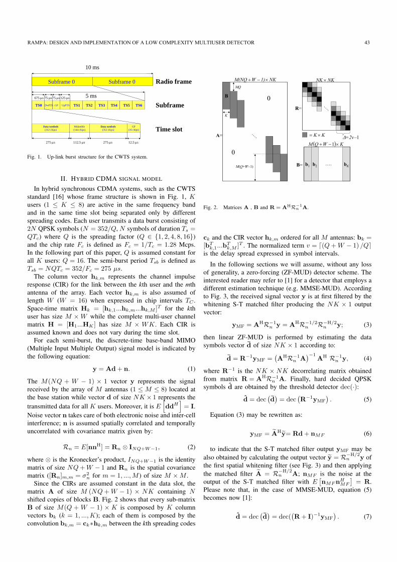
matrix A of size M (NQ + W − 1) × NK containing Nshifted copies of blocks B. Fig. 2 shows that every sub-matrixB of size M(Q + W − 1) × K is composed by K columnvectors bk (k = 1, ...,K); each of them is composed by theconvolution bk,m = ck∗hk,m between the kth spreading codes

��

�

��

�

��

�

�

��

��

��

��

��

��

� � ��

Fig. 2. Matrices A , B and R = AHR−1n A.

ck and the CIR vector hk,m ordered for all M antennas: bk =[bT

k,1...bTk,M ]T . The normalized term v = d(Q + W − 1) /Qe

is the delay spread expressed in symbol intervals.

In the following sections we will assume, without any lossof generality, a zero-forcing (ZF-MUD) detector scheme. Theinterested reader may refer to [1] for a detector that employs adifferent estimation technique (e.g. MMSE-MUD). Accordingto Fig. 3, the received signal vector y is at first filtered by thewhitening S-T matched filter producing the NK × 1 outputvector:

yMF = AHR−1n y = AHR−1/2

n R−H/2n y; (3)

then linear ZF-MUD is performed by estimating the datasymbols vector d of size NK × 1 according to:

d = R−1yMF =(AHR−1

n A)−1

AH R−1n y, (4)

where R−1 is the NK × NK decorrelating matrix obtainedfrom matrix R = AHR−1

n A. Finally, hard decided QPSKsymbols d are obtained by the threshold detector dec(·):

d = dec(d)

= dec(R−1yMF

). (5)

Equation (3) may be rewritten as:

yMF = AHy= Rd + nMF (6)

to indicate that the S-T matched filter output yMF may bealso obtained by calculating the output vector y = R−H/2

n y ofthe first spatial whitening filter (see Fig. 3) and then applyingthe matched filter A = R−H/2

n A; nMF is the noise at theoutput of the S-T matched filter with E

[nMF nH

MF

]= R.

Please note that, in the case of MMSE-MUD, equation (5)becomes now [1]:

d = dec(d)

= dec((R + I)−1yMF

). (7)

RAMPA: DESIGN AND IMPLEMENTATION OF A LOW COMPLEXITY MULTIUSER DETECTOR 43

space-timewhitened

matched filterspace-time

detector

21H /RA −n

1

M

M

1

K

M

1

K

M

1

M

y

1−R

whiteningfilter

2H /R−n

M

Space-time MUD

d

threshold detector

1

K

Mdec

dMFy

Fig. 3. Block diagram of the S-T ZF-MUD.

III. EFFICIENT DETECTOR ALGORITHMS

Most of the complexity of the linear detector algorithmsemployed for MUD scheme proposed in the previous sectionarises from the inversion methods of the large correlationmatrix R and from the matched filter computation [8]. Asdepicted in Fig. 2, matrix R is block-Toeplitz and block-banded. It is composed by N × N sub-matrices Ri (i =0, ..., N − 1) having size K ×K:

R =

R0 R−1 . . . R−(N−1)

R1 R0 . . . . . .. . . . . . . . . R−1

R(N−1) . . . R1 R0

, (8)

where R−i = RHi (i = 1, ..., N −1). Moreover, matrix R has

only 2v − 1 non null block-diagonals: R−i = RHi = 0, for

i = v, v + 1, ..., N − 1.As far as the matched filter output yMF is concerned, its

computational cost dominates using an antenna array (M >>1); however its calculation has a high degree of parallelism thatcan be easily exploited during the hardware implementation(e.g. using a polyphase Q-decimated filter bank) [8].

Some MUD algorithms compute directly the decorrelatingmatrix R−1 and then calculate the solution (4) by matrixmultiplication. On the contrary, other algorithms factorizematrix R and then solve the equation:

Rd = yMF. (9)

While the block-Levinson algorithm [14] belongs to the firstclass of techniques, the latter family includes the well knownblock-Fourier (BFT) [17] algorithm and all methods derivedfrom the QR decomposition [18] of the matrix R. To thissecond family belongs also the block-Bareiss algorithm thatwill be discussed later on.

All the methods that belong to the second family are similarto the plain Cholesky algorithm and differ only in the usedfactorization algorithm that takes care of the block-Toeplitzmatrix R having in common the remaining processing steps.For instance, the Cholesky algorithm computes the Choleskyfactor U of the matrix R: R = UHU. Then, both the lowertriangular system:

UHz = yMF (10)

and the upper triangular one:

Ud = z, (11)

are computed sequentially by using the backward and for-ward (B/F) algorithm, respectively. The Cholesky factor U

of a block-Toeplitz matrix R is block-banded but not block-Toeplitz. However, the Cholesky factor structure shown in[19] may be exploited to approximate the factorization andto speed-up the computation if N >> v. This approximationmay be used together with the well known generalized Schuralgorithm [17] to speed up the whole computation. It is worthmentioning that the B/F algorithm has a complexity in theorder of O[N2K2].

A. Factorization algorithms

The exact computation of the Cholesky factor U for aarbitrary NK×NK matrix R requires a number of operationsin the order of O[N3K3] that is prohibitive for a large numberof symbols N and/or users K. For this reason, several fastinversion or factorization algorithms have been developed.

B. Block-Fourier algorithm

The BFT algorithm [4] is derived from the plain Fourieralgorithm briefly recalled here. The Fourier technique solvesthe generic problem:

Rx = y, (12)

where ∀h, k = 0, ..., n − 1 it is [R]h,k = rh,k, rh,k dependsonly on the difference k − h and rh,h = r0. The solution iscomputed by transforming equation (12) into the frequencydomain by exploiting the nth order DFT matrix operator Fdefined as:

[F]h,k = exp {−j2π(h− 1)(k − 1)/n} , (13)

where n is the problem size and h, k = 1, ..., n. If the matrixR is circulant, then it is well known [18] that R may befactorized as:

R = F−1ΛF, (14)

where the matrix Λ is the diagonal matrix containing theeigenvalues of R. It may be noticed that if A is circulantthen R is circulant, too.

The convolution problem (12) becomes now:

FRx = ΛFx = Fy, (15)

while the solution vector x is obtained by inverse DFTtransformation F−1:

x = F−1Λ−1Fy. (16)

The Fourier method is computationally effective because thediagonal matrix Λ, that contains the eigenvalues of R, can beefficiently computed by transforming only the first column r1

of the matrix R according to:

λ = Fr1, (17)

where column vector λ is obtained from eigenvalue matrixΛ by rearranging its diagonal elements by means of the diagoperator:

λ = diag (Λ) = Λ 1n (18)

and 1n is the column vector of length n having all terms equalto one.


DK

DP

K

P

B

B

B

O

AAC

~

~

B

B

B

B

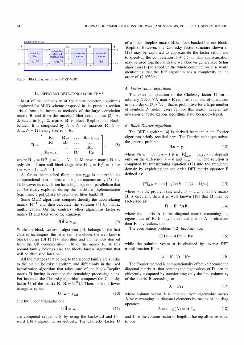
Fig. 4. Structure of circulant matrix eAc used by the Block-Fourier algorithm.The matrix size is DP ×DK where D = N + v − 1 and P = MQ. It isalso indicated the original matrix eA.

Unfortunately, the matrix R is not circulant, it is also block-Toeplitz and block-band but it has only 2v−1 non null block-diagonals (Fig. 2). It may be easily made circulant with fewmodifications: the circulant block matrix Ac is obtained fromA just adding and arranging columns of blocks as shown inFig. 4. The number of added blocks depend on the value v:in our case, the matrix Ac has size DP × DK where D =N +v−1 and P = MQ while circulant matrix Rc = AH

c Ac,derived from Ac, has size DK ×DK.

Now, the plain Fourier algorithm must be modified to handlethe block-circulant matrix Rc containing D2 blocks of sizeK ×K. Instead of the Fourier matrix (13), now it is definedthe block-Fourier matrix transformation F(K) = F⊗IK where⊗ is the Kronecker’s product, IK is the K × K identitymatrix, FK and F represent the Kth and the Dth order DFT,respectively.

The equation equivalent to (14) is:

Rc = F−1(K)Λ(K)F(K), (19)

where Λ(K) is the block-diagonal matrix composed of D nonnull blocks of size K × K along the main block-diagonal. Itis computed (cf. Eq.17):

diag(K)

(Λ(K)

)= F(K)Rc1, (20)

where Rc1 is the first block column of the matrix Rc anddiag(K) (·) is the extension of the diag operator (18) to theK ×K block size case.

Finally, the BFT algorithm computes the following matrixequation corresponding to (15):

F(K)d = Λ−1(K)F(K)yMF (21)

and then applying the inverse DFT operator F−1(K):

d = F−1(K)Λ

−1(K)F(K)yMF . (22)

The block elements of block-diagonal matrix Λ(K) haveno particular structure; therefore Λ−1

(K) may be obtained withstandard (or approximated) methods such as the Choleskyfactorization. In addition, the matched filter output yMF isobtained from equation (6). Only the first NK values of dfrom the equation (22) are used to compute the vector d.

It is possible to speed up the block-Fourier algorithm byreducing the ideal length D of the FFT (i.e. using optimizedradix-4 operators) with respect to the true value N + v − 1and by using the well-known overlap-and-save technique. Itrequires the use of L = dN/ (D − prelap−postlap)e datavector slices of reduced size D to cover N symbols [4].

C. Block-Levinson algorithm

The BL algorithm is derived from the plain Levinson algo-rithm that computes the direct problem Rx = y by invertingthe matrix R that is Hermitian, Toeplitz and positive defined.For a generic matrix R of size n×n, this technique requires anumber of operations in the order of O[n2]. The BL algorithmhas been extended [14],[20] to the block-Toeplitz matrices R(i)

of size NK × NK by solving the following system at stepi + 1:

R(i+1)d(i+1) = y(i+1)MF (23)

starting from the solution at step i. The original problem (9)is solved through N − 1 iterations. By defining matrix R(i)

as:

R(i) =

R0 R−1 . . . R−i

R1 R0 . . . . . .. . . . . . . . . R−1

Ri . . . R1 R0

, (24)

the system (23) may be rewritten as (1 ≤ i ≤ N − 1):[R(i) Ei

(G(i)

)T(G(i)

)TEi R0

] [d(i)

µ

]=

=

[y(i)

MF

y(i,i+1)MF

],

(25)

where d(i) and y(i)MF are sub-vectors of length iK obtained

from the vectors d and yMF, respectively. The vector y(i,i+1)MF ,

that is extracted from the matched filter output yMF, has sizeK× 1. Matrix G(i) is defined as G(i) =

[RT

1 RT2 ...RT

i

]T, Ei

is the exchange block matrix of size iK × iK that inverts theorder of the blocks of the previous matrix G(i) and µ is anauxiliary vector [14] of size K × 1.

As indicated in the BFT algorithm, it is also possible toincrease the algorithm processing speed by considering that,after few iterations, some internal parameters converge rapidlyto their final value and may therefore considered constant.Reference [4] shows a detailed description about these op-timizations.

D. Block-Bareiss algorithm

The plain Bareiss algorithm [13] employs an iterative tech-nique, derived from the classical Schur algorithm, to solve a


OO

1

3

2

3

3

3

( ) =+3ROO

1

2

3

3

3

3

( ) =−3R

0

0

0

0

0

0

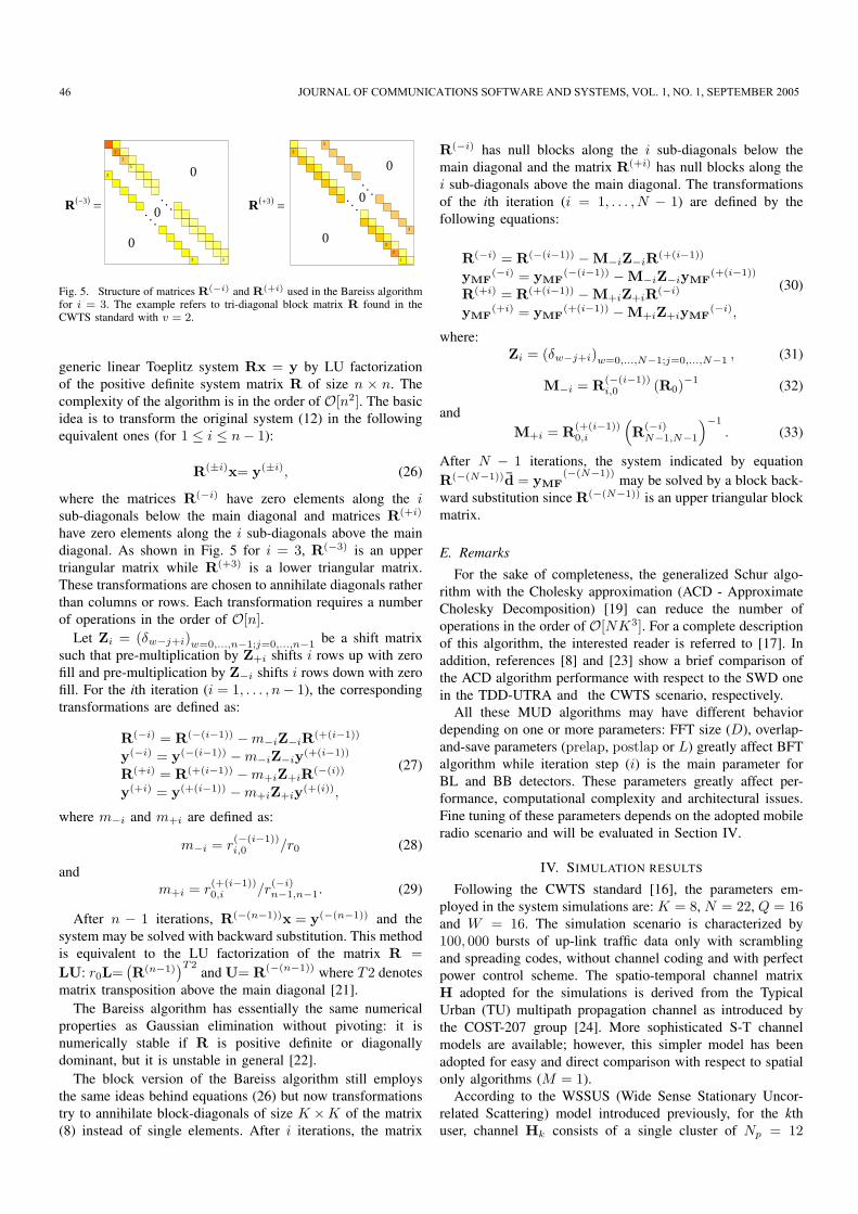
Fig. 5. Structure of matrices R(−i) and R(+i) used in the Bareiss algorithmfor i = 3. The example refers to tri-diagonal block matrix R found in theCWTS standard with v = 2.

generic linear Toeplitz system Rx = y by LU factorizationof the positive definite system matrix R of size n × n. Thecomplexity of the algorithm is in the order of O[n2]. The basicidea is to transform the original system (12) in the followingequivalent ones (for 1 ≤ i ≤ n− 1):

R(±i)x= y(±i), (26)

where the matrices R(−i) have zero elements along the isub-diagonals below the main diagonal and matrices R(+i)

have zero elements along the i sub-diagonals above the maindiagonal. As shown in Fig. 5 for i = 3, R(−3) is an uppertriangular matrix while R(+3) is a lower triangular matrix.These transformations are chosen to annihilate diagonals ratherthan columns or rows. Each transformation requires a numberof operations in the order of O[n].

Let Zi = (δw−j+i)w=0,...,n−1;j=0,...,n−1 be a shift matrixsuch that pre-multiplication by Z+i shifts i rows up with zerofill and pre-multiplication by Z−i shifts i rows down with zerofill. For the ith iteration (i = 1, . . . , n− 1), the correspondingtransformations are defined as:

R(−i) = R(−(i−1)) −m−iZ−iR(+(i−1))

y(−i) = y(−(i−1)) −m−iZ−iy(+(i−1))

R(+i) = R(+(i−1)) −m+iZ+iR(−(i))

y(+i) = y(+(i−1)) −m+iZ+iy(+(i)),

(27)

where m−i and m+i are defined as:

m−i = r(−(i−1))i,0 /r0 (28)

andm+i = r

(+(i−1))0,i /r

(−i)n−1,n−1. (29)

After n − 1 iterations, R(−(n−1))x = y(−(n−1)) and thesystem may be solved with backward substitution. This methodis equivalent to the LU factorization of the matrix R =LU: r0L=

(R(n−1)

)T2and U= R(−(n−1)) where T2 denotes

matrix transposition above the main diagonal [21].The Bareiss algorithm has essentially the same numerical

properties as Gaussian elimination without pivoting: it isnumerically stable if R is positive definite or diagonallydominant, but it is unstable in general [22].

The block version of the Bareiss algorithm still employsthe same ideas behind equations (26) but now transformationstry to annihilate block-diagonals of size K ×K of the matrix(8) instead of single elements. After i iterations, the matrix

R(−i) has null blocks along the i sub-diagonals below themain diagonal and the matrix R(+i) has null blocks along thei sub-diagonals above the main diagonal. The transformationsof the ith iteration (i = 1, . . . , N − 1) are defined by thefollowing equations:

R(−i) = R(−(i−1)) −M−iZ−iR(+(i−1))

yMF(−i) = yMF

(−(i−1)) −M−iZ−iyMF(+(i−1))

R(+i) = R(+(i−1)) −M+iZ+iR(−i)

yMF(+i) = yMF

(+(i−1)) −M+iZ+iyMF(−i),

(30)

where:Zi = (δw−j+i)w=0,...,N−1;j=0,...,N−1 , (31)

M−i = R(−(i−1))i,0 (R0)

−1 (32)

andM+i = R(+(i−1))

0,i

(R(−i)

N−1,N−1

)−1

. (33)

After N − 1 iterations, the system indicated by equationR(−(N−1))d = yMF

(−(N−1)) may be solved by a block back-ward substitution since R(−(N−1)) is an upper triangular blockmatrix.

E. Remarks

For the sake of completeness, the generalized Schur algo-rithm with the Cholesky approximation (ACD - ApproximateCholesky Decomposition) [19] can reduce the number ofoperations in the order of O[NK3]. For a complete descriptionof this algorithm, the interested reader is referred to [17]. Inaddition, references [8] and [23] show a brief comparison ofthe ACD algorithm performance with respect to the SWD onein the TDD-UTRA and the CWTS scenario, respectively.

All these MUD algorithms may have different behaviordepending on one or more parameters: FFT size (D), overlap-and-save parameters (prelap, postlap or L) greatly affect BFTalgorithm while iteration step (i) is the main parameter forBL and BB detectors. These parameters greatly affect per-formance, computational complexity and architectural issues.Fine tuning of these parameters depends on the adopted mobileradio scenario and will be evaluated in Section IV.

IV. SIMULATION RESULTS

Following the CWTS standard [16], the parameters em-ployed in the system simulations are: K = 8, N = 22, Q = 16and W = 16. The simulation scenario is characterized by100, 000 bursts of up-link traffic data only with scramblingand spreading codes, without channel coding and with perfectpower control scheme. The spatio-temporal channel matrixH adopted for the simulations is derived from the TypicalUrban (TU) multipath propagation channel as introduced bythe COST-207 group [24]. More sophisticated S-T channelmodels are available; however, this simpler model has beenadopted for easy and direct comparison with respect to spatialonly algorithms (M = 1).

According to the WSSUS (Wide Sense Stationary Uncor-related Scattering) model introduced previously, for the kthuser, channel Hk consists of a single cluster of Np = 12


-10 -5 0 5 10 15 2010

-6

10-5

10-4

10-3

10-2

10-1

100

BER

pre=0, post=0pre=1, post=0pre=0, post=1pre=1, post=1pre=2, post=1pre=1, post=2exact inversion

-10 -5 0 5 10 15 2010

-6

10-5

10-4

10-3

10-2

10-1

100

BER

pre=0, post=0pre=3, post=2pre=3, post=3;pre=4, post=4;pre=5, post=5exact inversion

BFT DetectorD = 4, M = 1

BFT DetectorD = 16, M = 1

BER

-10 -5 0 5 10 15 2010

-6

10-5

10-4

10-3

10-2

10-1

100

SNR [dB]

BER

i = 1i = 2i > 2exact inversion

BL DetectorM = 1

-10 -5 0 5 10 15 2010

-6

10-5

10-4

10-3

10-2

10-1

100

SNR [dB]

i = 1i = 2i > 2exact inversion

BB DetectorM = 1

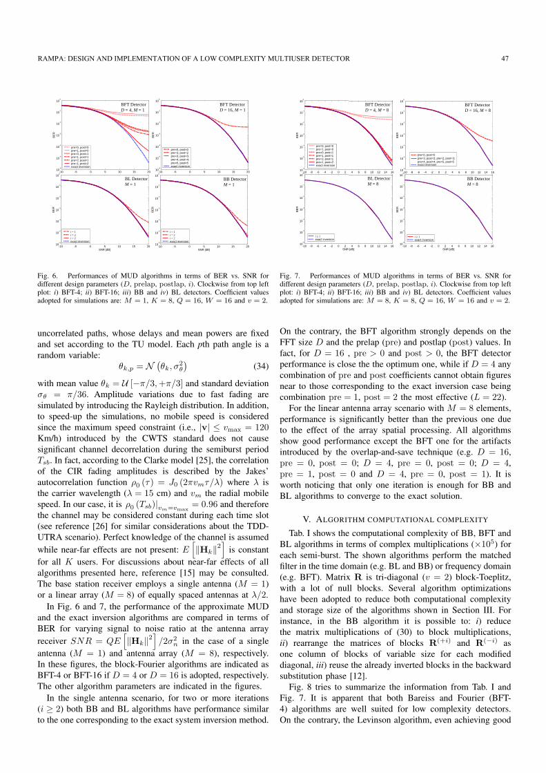
Fig. 6. Performances of MUD algorithms in terms of BER vs. SNR fordifferent design parameters (D, prelap, postlap, i). Clockwise from top leftplot: i) BFT-4; ii) BFT-16; iii) BB and iv) BL detectors. Coefficient valuesadopted for simulations are: M = 1, K = 8, Q = 16, W = 16 and v = 2.

uncorrelated paths, whose delays and mean powers are fixedand set according to the TU model. Each pth path angle is arandom variable:

θk,p = N(θk, σ2

θ

)(34)

with mean value θk = U [−π/3,+π/3] and standard deviationσθ = π/36. Amplitude variations due to fast fading aresimulated by introducing the Rayleigh distribution. In addition,to speed-up the simulations, no mobile speed is consideredsince the maximum speed constraint (i.e., |v| ≤ vmax = 120Km/h) introduced by the CWTS standard does not causesignificant channel decorrelation during the semiburst periodTsb. In fact, according to the Clarke model [25], the correlationof the CIR fading amplitudes is described by the Jakes’autocorrelation function ρ0 (τ) = J0 (2πvmτ/λ) where λ isthe carrier wavelength (λ = 15 cm) and vm the radial mobilespeed. In our case, it is ρ0 (Tsb)|vm=vmax

= 0.96 and thereforethe channel may be considered constant during each time slot(see reference [26] for similar considerations about the TDD-UTRA scenario). Perfect knowledge of the channel is assumedwhile near-far effects are not present: E

[‖Hk‖2

]is constant

for all K users. For discussions about near-far effects of allalgorithms presented here, reference [15] may be consulted.The base station receiver employs a single antenna (M = 1)or a linear array (M = 8) of equally spaced antennas at λ/2.

In Fig. 6 and 7, the performance of the approximate MUDand the exact inversion algorithms are compared in terms ofBER for varying signal to noise ratio at the antenna arrayreceiver SNR = QE

[‖Hk‖2

]/2σ2

n in the case of a singleantenna (M = 1) and antenna array (M = 8), respectively.In these figures, the block-Fourier algorithms are indicated asBFT-4 or BFT-16 if D = 4 or D = 16 is adopted, respectively.The other algorithm parameters are indicated in the figures.

In the single antenna scenario, for two or more iterations(i ≥ 2) both BB and BL algorithms have performance similarto the one corresponding to the exact system inversion method.

BFT Detector D = 4, M = 8

-10 -8 -6 -4 -2 0 2 4 6 8 10 12 14 1610

-6

10-5

10-4

10-3

10-2

10-1

100

BER

pre=0, post=0pre=1, post=0pre=0, post=1pre=1, post=1pre=2, post=1pre=1, post=2exact inversion

0

BFT Detector D = 16, M = 8

-10 -8 -6 -4 -2 0 2 4 6 8 10 12 14 1610

-6

10-5

10-4

10-3

10-2

10-1

10

pre=3, post=2; pre=2, post=3;pre=4, post=4; pre=5, post=5exact inversion

pre=0, post=0

BER

BER

-10 -8 -6 -4 -2 0 2 4 6 8 10 12 14 1610

-6

10-5

10-4

10-3

10-2

10-1

100

SNR [dB]

i ≥ 1exact inversion

BL Detector M = 8

-10 -8 -6 -4 -2 0 2 4 6 8 10 12 14 1610

-6

10-5

10-4

10-3

10-2

10-1

100

SNR [dB]

BB Detector M = 8

i ≥ 1exact inversion

BER

Fig. 7. Performances of MUD algorithms in terms of BER vs. SNR fordifferent design parameters (D, prelap, postlap, i). Clockwise from top leftplot: i) BFT-4; ii) BFT-16; iii) BB and iv) BL detectors. Coefficient valuesadopted for simulations are: M = 8, K = 8, Q = 16, W = 16 and v = 2.

On the contrary, the BFT algorithm strongly depends on theFFT size D and the prelap (pre) and postlap (post) values. Infact, for D = 16 , pre > 0 and post > 0, the BFT detectorperformance is close the the optimum one, while if D = 4 anycombination of pre and post coefficients cannot obtain figuresnear to those corresponding to the exact inversion case beingcombination pre = 1, post = 2 the most effective (L = 22).

For the linear antenna array scenario with M = 8 elements,performance is significantly better than the previous one dueto the effect of the array spatial processing. All algorithmsshow good performance except the BFT one for the artifactsintroduced by the overlap-and-save technique (e.g. D = 16,pre = 0, post = 0; D = 4, pre = 0, post = 0; D = 4,pre = 1, post = 0 and D = 4, pre = 0, post = 1). It isworth noticing that only one iteration is enough for BB andBL algorithms to converge to the exact solution.

V. ALGORITHM COMPUTATIONAL COMPLEXITY

Tab. I shows the computational complexity of BB, BFT andBL algorithms in terms of complex multiplications (×105) foreach semi-burst. The shown algorithms perform the matchedfilter in the time domain (e.g. BL and BB) or frequency domain(e.g. BFT). Matrix R is tri-diagonal (v = 2) block-Toeplitz,with a lot of null blocks. Several algorithm optimizationshave been adopted to reduce both computational complexityand storage size of the algorithms shown in Section III. Forinstance, in the BB algorithm it is possible to: i) reducethe matrix multiplications of (30) to block multiplications,ii) rearrange the matrices of blocks R(+i) and R(−i) asone column of blocks of variable size for each modifieddiagonal, iii) reuse the already inverted blocks in the backwardsubstitution phase [12].

Fig. 8 tries to summarize the information from Tab. I andFig. 7. It is apparent that both Bareiss and Fourier (BFT-4) algorithms are well suited for low complexity detectors.On the contrary, the Levinson algorithm, even achieving good


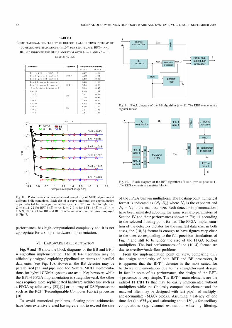
TABLE ICOMPUTATIONAL COMPLEXITY OF DETECTOR ALGORITHMS IN TERMS OF

COMPLEX MULTIPLICATIONS (×105) PER SEMI-BURST. BFT-4 AND

BFT-16 INDICATE THE BFT ALGORITHM WITH D = 4 AND D = 16,RESPECTIVELY.

Parameters Algorithm Computational complexity

M = 1 M = 8

L = 4, pre = 5, post = 5

L = 3, pre = 4, post = 4

L = 2, pre = 2, post = 3

BFT-160.27

0.22

0.18

1.19

1.01

0.83

L = 22, pre = 2, post = 1

L = 11, pre = 1, post = 1

L = 6, pre = 0, post = 0

BFT-40.25

0.14

0.09

1.19

0.68

0.45

i = 21

i = 5

i = 3

i = 1

BB

1.43

0.41

0.28

0.15

1.97

0.94

0.82

0.69

i = 21

i = 5

i = 3

i = 1

BL

3.68

1.06

0.91

0.81

4.21

1.59

1.45

1.34

0.4 0.6 0.8 1 1.2 1.4 1.6 1.8 2 2.210

-6

10-5

10-4

10-3

10-2

10-1

Complex multiplications [x 105]

BE

R

M = 8

SNR = 8 dB

SNR = 10dB

SNR = 12dB

SNR = 14dB

SNR = 16dB

BFT-4BLBB

BFT-16SNR = 6 dB

Fig. 8. Performances vs. computational complexity of MUD algorithms atdifferent SNR conditions. Each dot of a curve indicates the approximationdegree adopted for the algorithm at that specific SNR. From left to right it is:L = 6, 11, 22 for BFT-4 (D = 4), L = 2, 3, 4 for BFT-16 (D = 16), i =1, 5, 9, 13, 17, 21 for BB and BL. Simulation values are the same employedin Fig. 7.

performance, has high computational complexity and it is notappropriate for a simple hardware implementation.

VI. HARDWARE IMPLEMENTATION

Fig. 9 and 10 show the block diagrams of the BB and BFT-4 algorithm implementation. The BFT-4 algorithm may beefficiently designed exploiting pipelined structures and paralleldata units (see Fig. 10). However, the BB detector may beparallelized [21] and pipelined, too. Several MUD implementa-tions for hybrid CDMA systems are available; however, whilethe BFT-4 FPGA implementation is straightforward, the otherones requires more sophisticated hardware architecture such asa FPGA systolic array [23],[9] or an array of DSP/processorssuch as the RCF (Reconfigurable Computer Fabric) processor[10].

To avoid numerical problems, floating-point arithmeticshave been extensively used having care not to exceed the size

Polyphasematched filter

y

Ac

yMF

Rc(1,1)

TR

Rccomputation

RE

G

REG

Inversionprocessor

Bareissloop

Partial back-substitutionprocessor

dRc(1,1)−1

Fig. 9. Block diagram of the BB algorithm (i = 1). The REG elements areregister blocks.

Rccomputation

FFT- 4radix 4

Matched Filter

Choleskyprocessor

BF substitutionprocessor

y

d

RE

G

REG

RE

GRE

GR

EG

D

Rc

FFT- 4radix 4

FFT- 4radix 4

Ac

IFFT- 4radix 4

YMF

Fig. 10. Block diagram of the BFT algorithm (D = 4, pre = post = 1).The REG elements are register blocks.

of the FPGA built-in multipliers. The floating-point numericalformat is indicated as (Nt, Ne) where Ne is the exponent andNt − Ne is the mantissa size. Both detector implementationshave been simulated adopting the same scenario parameters ofSection IV and their performances shown in Fig. 11 accordingto the selected floating-point format. The FPGA implementa-tion of the detectors dictates for the smallest data size: in bothcases, the (10, 5) format is enough to have figures very closeto the ones corresponding to the full precision simulations ofFig. 7 and still to be under the size of the FPGA built-inmultipliers. The bad performances of the (10, 4) format aredue to overflow/underflow problems.

From the implementation point of view, comparing onlythe design complexity of both BFT and BB processors, itis apparent that the BFT-4 detector is the most suited forhardware implementation due to its straightforward design.In fact, in spite of its performance, the design of the BFT-4 processor is very simple. The BFT-4 main elements are theradix-4 FFT/IFFTs that may be easily implemented withoutmultipliers while the Cholesky computation element and thematched filter may be designed with fast pipelined multiply-and-accumulate (MAC) blocks. Assuming a latency of onetime slot (i.e. 675 µs) and estimating about 180 µs for ancillarycomputations (e.g. channel estimation, whitening filtering,


0 5 10 15 2010-5

10-4

10-3

10-2

10-1

100

BFT-4 Detector D = 4, M = 8pre = 1, post =1

SNR [dB]

BE

R(10, 4)( 9, 5)(10, 5)(12, 5)(32, 8)

0 5 10 15 2010-5

10-4

10-3

10-2

10-1

100

SNR [dB]

BE

R

(10, 4)( 9, 5)(10, 5)(12, 5)(32, 8)

BB Detector M = 8, i = 3

Fig. 11. Performance changes due to the floating-point numerical format(Nt, Ne) adopted for the algorithm implementations. From left to right: i)BB (i = 3) and ii) BFT-4 (D = 4, pre = post = 1) performances vs.numeric formats. The simulation results correspond to the block diagrams ofFig. 9 and 10.

33

33

25

25

30

30

34

34

24

25

32

32

31

31

26

27

27

28

33

33

26

26

29

29

29

28

28

28

30

30

34

34

25

25

32

32

31

31

27

27

34

33

33

33

26

26

32

32

31

30

28

28

29

29

33

33

30

29

31

31

32

32

27

27

29

29

34

34

25

25

30

30

31

31

26

26

28

29

33

33

27

27

32

32

31

31

24

24

34

34

33

34

25

25

32

32

30

30

26

27

29

29

34

33

28

28

31

31

32

32

30

30

27

26

31

31

34

33

28

28

29

29

A32

32

25

25

34

33

A34

34

24

24

30

A30

A33

33

29

28

A31

31

A29

29

27

27

31

31

34

34

26

A26

32

32

33

33

25

A25

A27

27

33

34

28

28

33

33

29

29

26

26

30

30

34

34

27

27

32

31

33

33

25

25

32

32

31

31

26

26

28

28

K34

L34

27

27

29

29

30

30

28

28

32

32

K33

L33

26

26

29

29

K31

31

25

25

K32

L32

30

30

25

24

E2

D2

K1

K1

F5

G5

E3

D3

J9

K9

F4

E4

E1

D1

J8

K8

H7

J7

H6

G6

L1

L9

G3

F3

G2

F2

M1

N1

J6

K6

J5

H5

L7

K7

J4

H4

G1

F1

L8

M8

J1

H2

J3

H3

M9

N9

L5

K5

K2

J2

N7

M7

L6

M6

M3

L3

L4

K4

N4

M4

M2

L2

N8

P8

N6

P6

P5

N5

P1

R1

P3

N3

M1

L1

P9

R9

P2

N2

R4

P4

R8

T8

T3

R3

P1

N1

T1

U1

R7

R6

U5

T5

T1

U1

U4

T4

T2

R1

U7

T7

T6

U6

U1

U2

U9

U8

U3

V4

V6

W6

V5

W5

V7

W7

V1

W

V1

V2

W3

Y3

V9

V8

W4

Y4

W

V1

W8

Y8

W2

Y1

AA

AB

Y6

AA

AA

AB

Y7

AA

Y1

AA

AA

AB

AA

AB

AA

Y9

AA

AB

AB

AC

AD

AC

AC

AD

AC

AD

AB

AC

AC

AD

AC

AB

AB

AC

AD

AE

AE

AF

AB

AC

AE

AF

AD

AE

AD

AE

AF

AG

AF

AG

AD

AE

AF

AG

AE

AD

AF

AF

AH

AJ

AG

AH

AF

AG

AH

AJ

AF

AG

AL

AK

AH

AJ

AJ

AK

AE

AD

AK

AL

AH

AJ

AE

AF

AK

AL

AF

AG

F9

F8

H10

H9

C2

B3

D10

D11

G12

G13

B9

B10

B8

A9

K14

K13

A6

A7

D9

C9

H13

H12

C7

C8

E11

E10

J13

K12

B6

B7

E8

E9

G10

G11

A4

A5

F10

G9

J12

J11

B4

B5

D6

C6

H11

J10

D8

E7

F16

F17

G16

G17

C16

C15

D14

D15

J17

K17

B17

A17

A15

B16

L17

L16

A13

A14

C13

C14

K16

K15

B13

B14

F15

G15

H15

H14

A11

A12

E13

E14

J15

J14

D12

D13

F14

F13

C11

C12

B11

B12

F11

F12

C19

C18

K18

J18

E19

E18

E17

E16

H17

H16

D17

D16

B25

B26

B23

B24

G22

G23

F22

F21

A23

A24

K21

K20

C22

C23

E21

E22

H21

H20

G20

F20

B21

B22

J20

K19

D20

D21

A21

A22

L19

L18

B19

A20

A18

B18

H19

H18

C20

C21

D19

D18

G18

G19

F18

F19

F25

F26

H25

H24

E26

F27

B32

C33

J24

J23

C27

C28

B30

B31

K23

K22

C26

D27

A30

A31

G24

G25

E25

E24

D25

D26

H23

H22

F23

F24

B28

B29

J22

J21

A28

A29

A26

B27

C24

D24

D22

D23

D29

C29

H26

G26

E28

E27

AK7

AK8

AM4

AL5

AG10

AH11

AM11

AL11

AP9

AN8

AG13

AG14

AJ11

AJ12

AP7

AP6

AH13

AH12

AK10

AK11

AL10

AL9

AF12

AF13

AN7

AN6

AP5

AP4

AG11

AG12

AM9

AL8

AN5

AN4

AE12

AE13

AH9

AH10

AN3

AM2

AJ10

AJ9

AM8

AM7

AL6

AM6

AK9

AJ8

AM15

AM14

AL16

AL17

AJ17

AJ16

AL15

AL14

AP17

AN17

AH17

AH16

AH15

AJ15

AN16

AP15

AE16

AE17

AK14

AK13

AP14

AP13

AD16

AD17

AN14

AN13

AP12

AP11

AG15

AG16

AM13

AM12

AL13

AL12

AF14

AF15

AJ13

AJ14

AN12

AN11

AE14

AE15

AN10

AN9

AL18

AL19

AK18

AK19

AG18

AF18

AF17

AG17

AK16

AK17

AM16

AM17

AN26

AN25

AJ24

AJ23

AN24

AN23

AJ21

AJ22

AF20

AF21

AM24

AM23

AL23

AL22

AG19

AG20

AP24

AP23

AJ20

AH20

AD18

AD19

AN22

AN21

AK22

AK21

AE18

AE19

AP22

AP21

AP20

AN19

AM22

AM21

AN18

AP18

AL21

AL20

AH19

AH18

AM19

AM20

AJ19

AJ18

AE22

AE23

AM28

AM29

AJ27

AJ26

AG23

AF24

AM33

AN32

AK26

AK27

AH26

AJ25

AN31

AN30

AL27

AL26

AF22

AF23

AM27

AM26

AH24

AH25

AH23

AH22

AP31

AP30

AK24

AK25

AG21

AG22

AN29

AN28

AP29

AP28

AE20

AE21

AN27

AP26

AL25

AL24

AG24

AG25

AL30

AM31

AK28

AL29

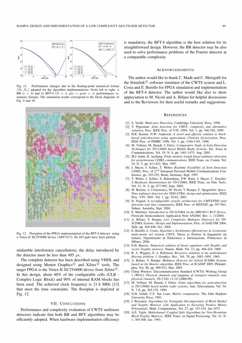
Fig. 12. Floorplan of the FPGA implementation of the BFT-4 detector usinga Virtex-II XC2V6000 device (-6FF1517). No I/O pads have been plotted.

midamble interference cancellation), the delay introduced bythe detector must be less than 495 µs.

The complete detector has been described using VHDL anddesigned using Mentor Graphics c© and Xilinx c© tools. Thetarget FPGA is the Virtex-II XC2V6000 device from Xilinx c©.In this design, about 60% of the configurable cells (CLB -Complex Logic Block) and 90% of internal RAM blocks hasbeen used. The achieved clock frequency is 21.8 MHz [12]that meet the time constraints. The floorplan is depicted inFig. 12.

VII. CONCLUSIONS

Performance and complexity evaluation of CWTS multiuserdetectors indicate that both BB and BFT algorithms may beefficiently adopted. When hardware implementation efficiency

is mandatory, the BFT-4 algorithm is the best solution for itsstraightforward design. However, the BB detector may be alsoused to solve performance problems of the Fourier detector ata comparable complexity.

ACKNOWLEDGMENTS

The author would like to thank C. Madè and C. Meregalli forthe Simulink c© software simulator of the CWTS system and L.Costa and E. Borello for FPGA simulation and implementationof the BFT-4 detector. The author would like also to showappreciation to M. Nicoli and A. Bifano for helpful discussionsand to the Reviewers for their useful remarks and suggestions.

REFERENCES

[1] S. Verdú: Multi-user Detection, Cambridge University Press, 1998.[2] Y. Pigeonnat: Joint detection for UMTS: complexity and alternative

solutions, Proc. IEEE Proc. of VTC 1999, Vol. 1, pp. 546-550, 1999.[3] H.R. Karimi, N.W. Anderson: A novel and efficient solution to block-

based joint-detection using approximate Cholesky factorization, Proc.IEEE Proc. of PIMRC 1998, Vol. 3, pp. 1340-1345, 1998.

[4] M. Vollmer, M. Haardt, J. Götze: Comparative Study of Joint-DetectionTechniques for TD-CDMA based Mobile Radio Systems, Sel. Areas inCommunications, Vol. 19, N. 8, pp. 1461-1475, Aug. 2001.

[5] M.J. Juntti, B. Aazhang: Finite memory length linear multiuser detectionfor asynchronous CDMA communications, IEEE Trans. on. Comm. Vol.54, N. 5, pp. 611-622, May 1997.

[6] J. Mayer, J. Schlee, T. Weber: Realtime Feasibility of Joint DetectionCDMA, Proc. of 2nd European Personal Mobile Communications Con-ference, pp. 245-252, Bonn, Germany, Sept. 1997.

[7] T. Weber, J. Schlee, S. Bahrenburg, P.W. Baier, J. Mayer, C. Euscher:A Hardware Demonstrator for TD-CDMA, IEEE Trans. on Vehi. Tech.,Vol. 51, N. 5, pp. 877-892, Sept. 2002.

[8] M. Beretta, A. Colamonico, M. Nicoli, V. Rampa, U. Spagnolini: Space-Time multiuser detectors for TDD-UTRA: design and optimization, IEEEProc. VTC 2001, Vol. 1, pp. 78-82, 2001.

[9] D. Noguet: A reconfigurable systolic architecture for UMTS/TDD jointdetection real time computation, IEEE Proc. of ISSSTAT, pp. 957-961,Sidney, Australia, Sept. 2004.

[10] E. Martinez: Introduction to TD-SCDMA on the MRC6011 RCF Device,Freescale Semiconductor Application Note AN2684, Rev. 1, 11/2004.

[11] A. Bifano, V. Rampa: Low Complexity Multiuser Detectors for TD-SCDMA Systems: Design and Implementation, Proc. of SoftCOM 2004,Split, pp. 444-448, Oct. 2004.

[12] E. Borello, L. Costa: Algoritmi e Architetture efficienti per la rivelazionemulti-utente nel sistema CWTS, Thesis as Dottore in Ingegneria (initalian), Dipartimento di Elettronica e Informazione, Politecnico diMilano, 2004.

[13] E.H. Bareiss: Numerical solution of linear equations with Toeplitz andvector Toeplitz matrices, Numer. Math. Vol. 13, pp. 404-424, 1969.

[14] R. A. Wiggins, E. A. Robinson: Recursive solutions to the multichannelfiltering problem, J. Geophys. Res., Vol. 70, pp. 1885–1891, 1965.

[15] A. Bifano, V. Rampa: Multiuser Detector for hybrid SCDMA Systemsbased on the Bareiss algorithm, IEEE Proc. of ICASSP 2005, Philadel-phia, Vol. III, pp. 909-912, Mar. 2005.

[16] China Wireless Telecommunication Standard (CWTS) Working Group1 (WG1): Physical channels and mapping of transport channels ontophysical channels, TS C102 v3.3.0 (2000-09).

[17] M. Vollmer, M. Haardt, J. Götze: Schur algorithms for joint-detectionin TD-CDMA based mobile radio systems, Ann. Telecommun. Vol. 54,N. 7-8, pp. 365-378, 1999.

[18] G.H. Golub, C.F. Van Loan: Matrix computation, The John HopkinsUniversity Press, 1991.

[19] J. Rissanen: Algorithms for Triangular Decomposition of Block Hankeland Toeplitz Matrices with Application to Factoring Positive MatrixPolynomials, Math. Computations, Vol. 27, pp. 147-154, Jan 1973.

[20] A.E. Yagle: Multichannel Coupled Split Algorithms for Non-HermitianBlock-Toeplitz Matrices, IEEE Trans. on Signal Processing, Vol. 41, N.1, 505-508, Jan. 1993.


[21] R.P. Brent: Parallel algorithms for Toeplitz systems, Numerical LinearAlgebra, Digital Signal Processing, Proc. NATO ASI, Leuven, Belgium,August 1988, edited by G. H. Golub and P. Van Dooren, NATO ASISeries F: Computer and Systems Sciences, Vol. 70, Springer-Verlag,1991.

[22] A.W. Bojanczyk, R.P. Brent, F.R. de Hoog and D.R. Sweet: On thestability of the Bareiss and related Toeplitz factorization algorithms,SIAM J. Matrix Analysis and Applications, Vol. 10, 225-244, 1995.

[23] A. Bifano, A. Colamonico, M. Nicoli, V. Rampa, U. Spagnolini: Slidingwindows multiuser detectors for TD-SCDMA systems, Proc. of EuropeanConference on Wireless Technology - ECWT ’02, Session E3, September2002.

[24] COST-207: Digital land mobile radio communications, Final Report,Luxemburg, Office for Official Publications of the European Communi-ties, 1989.

[25] G.L. Stuber: Principles of Mobile Communications, Kluwer Academic,1996.

[26] M. Nicoli, M. Sternad, U. Spagnolini, A. Ahlen, Reduced-rank channelestimation and tracking in time-slotted CDMA systems, Proc. IEEEInternational Conference on Communications (ICC ‘02), vol. 1, pp. 533-537, April-May 2002.

Vittorio Rampa was born in Genoa, Italy, in 1957.He received the Laurea (with Honors) as Dottore inIngegneria Elettronica in 1984 from the Politecnicodi Milano. In 1986 he joined the CSTS-CNR (Centerfor Space Communications) of the Italian NationalResearch Council (CNR) now IEIIT-CNR (Instituteof Electronics, Computer and TelecommunicationEngineering) where he is Senior Researcher. He wasa Visiting Scholar at Center for Integrated Systems,Stanford University during 1987-1988. Since 1999he is also Contract Professor at Politecnico di Milano

with research in telecommunication architectures. Presently, his researchinterests include signal processing for telecommunication and radar systemsand hardware/software reconfigurable architectures for mobile communicationsystems.


Documents

Design and Implementation of a Low Complexity Multiuser