Embed Size (px)
Citation preview

Design and implementation of a graph database for the storingof detected human mutations in the INGEMM
Student: Fernando Benito Valtueña
MÁSTER EN BIOINFORMÁTICA Y BIOLOGÍA COMPUTACIONALESCUELA NACIONAL DE SALUD- INSTITUTO DE SALUD CARLOS III
2013-2014
CENTRO/EMPRESA DONDE SE DESALLORARON LAS PRACTICAS: Instituto de Genética Médica y Molecular (INGEMM). Hospital La Paz. Madrid
DIRECTOR DE LA TESIS (TUTOR DE LA EMPRESA):Angela del Pozo Maté
CODIRECTOR DE LA TESIS (TUTOR POR EL MASTER):José María Fernández
FECHA: (MES Y AÑO DE LA PRESENTACION DE LA TESIS):October 2014
In first place I want to thank to the Máster de Bioinformática y Biología Computacional del Instituto de Salud Carlos III (ISCIII) and the INGEMM for the oportunity to accomplish this project.
Very specially to Angela del Pozo Mate and José María Fernández for all the guidance during the internship.
To Juan Carlos Silla-Castro and Kristina Ibáñez for all the assistance, the support and good advices and the good times with them.
To the rest of people in the INGEMM, specially to the GEF department (Elena Vallespín and Victoria E. M-Montaño)
Finally to all my classmates in the master because of their support.
Page 2
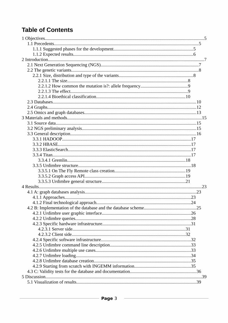
Table of Contents1 Objectives..........................................................................................................................................5
1.1 Precedents.............................................................................................................................51.1.1 Suggested phases for the development.....................................................................51.1.2 Expected results........................................................................................................6
2 Introduction.......................................................................................................................................72.1 Next Generation Sequencing (NGS).....................................................................................72.2 The genetic variants..............................................................................................................8
2.2.1 Size, distribution and type of the variants................................................................82.2.1.1 The size........................................................................................................82.2.1.2 How common the mutation is?: allele frequency.........................................92.2.1.3 The effect......................................................................................................92.2.1.4 Bioethical classification.............................................................................10
2.3 Databases............................................................................................................................102.4 Graphs.................................................................................................................................122.5 Omics and graph databases.................................................................................................13
3 Materials and methods.....................................................................................................................153.1 Source data..........................................................................................................................153.2 NGS preliminary analysis...................................................................................................153.3 General description.............................................................................................................16
3.3.1 HADOOP................................................................................................................173.3.2 HBASE...................................................................................................................173.3.3 ElasticSearch...........................................................................................................173.3.4 Titan........................................................................................................................17
3.3.4.1 Gremlin.......................................................................................................183.3.5 Urdimbre structure..................................................................................................18
3.3.5.1 On The Fly Remote class creation.............................................................193.3.5.2 Graph access API.......................................................................................193.3.5.3 Urdimbre general structure.........................................................................21
4 Results.............................................................................................................................................234.1 A: graph databases analysis.................................................................................................23
4.1.1 Approaches.............................................................................................................234.1.2 Final technological approach..................................................................................24
4.2 B: Implementation of the database and the database scheme.............................................254.2.1 Urdimbre user graphic interface.............................................................................264.2.2 Urdimbre queries....................................................................................................284.2.3 Specific hardware infrastructure.............................................................................31
4.2.3.1 Server side..................................................................................................314.2.3.2 Client side...................................................................................................32
4.2.4 Specific software infrastructure..............................................................................324.2.5 Urdimbre command line description......................................................................334.2.6 Urdimbre multiple use cases...................................................................................334.2.7 Urdimbre loading....................................................................................................344.2.8 Urdimbre database creation....................................................................................354.2.9 Starting from scratch with INGEMM information.................................................35
4.3 C: Validity tests for the database and documentation.........................................................365 Discussion........................................................................................................................................39
5.1 Visualization of results........................................................................................................39
Page 3
5.2 Scheme database.................................................................................................................395.3 Mutations graph style..........................................................................................................395.4 Advantages and limitations of graph database approach....................................................405.5 Multithreading.....................................................................................................................405.6 Sharding..............................................................................................................................40
6 Conclusions.....................................................................................................................................416.1 Future uses and improvements............................................................................................41
7 Bibliography....................................................................................................................................438 Annexes...........................................................................................................................................46
8.1 Highlights in the source code..............................................................................................46
Page 4
1 Objectives
Design and implementation of a graph oriented database for the storing of in INGEMM detected human mutations.
1.1 Precedents
With the idea of using NGS as a diagnostic test by the late of 2012 it is created the Bioinformatics section in INGEMM. Currently the equipment consists of three bioinformaticians.The project is now in an establishment phase. A cohort of patients properly phenotyped have been sequenced with the objective of establishing a genetic diagnostic based in NGS data and validated with Sanger sequencing [14].The section has an analysis pipeline developed completely in the INGEMM built with the more used open software tools in the NGS area. The variant that this pipeline characterizes are: isolated changes (SNVs), short insertions and deletions (indels) and copy number variations from at least 100 bases [14].One of the biggest difficulties in the massive sequencing (NGS) in the clinical routine is to assure the reliability of deleterious variants in order to establish them as associated or source of the patient's phenotype. It is also very important to determine common changes in the population (polymorphism) as well as possible artifacts appearing in a systematic way [14].Today there are not available variant databases of Spanish healthy population that can be used as controls in order to make easier the variant screening previously presented. Therefore, in order to improve the clinical practice, the information acquired throughout the years in the INGEMM is veryvaluable.Other important task is to know the allelic frequency of the polymorphisms characteristic in the Spanish population with the purpose of establishing the line between common and rare changes.
Therefore it is necessary to compile in a single database all the variants detected on the studied patients. In addition, the database could be explored in order to provide information to progress in the knowledge of the mutations associated to several pathologies, mainly in those in which the INGEMM is a reference center [14].
The objective intended is the creation of a database with the mutations detected in the INGEMM. A graph oriented database (NoSQL) is intended, since it permits the modeling of complex relationships between data and is easily scalable. It is predictable a fast increase of the variants to store because the growing of the number of patients.
1.1.1 Suggested phases for the development
It is intended a project duration of four months and the proposal is structured in these tasks:
Page 5
A. Study of the state of the art in graph databases: some software (HBASE, Cassandra, Neo4j, etc) will be reviewed. Then the most suitable implementation will be selected. At the end of this phase a brief document will be written.
B. Implementation of a graph oriented database. With the INGEMM staff pathology with a big number of patients will be selected as a model. This pathology will be complex genetically based, but known. That pathology will be used as reference for the database implementation.
C. Review of the prototype validity and documentation. The implementation will be validated with other pathologies.
1.1.2 Expected resultsIt is expected to do a study of the state of art of the graph oriented databases and a design and an implementation of a prototype using the variants of the model pathology. That prototype and the documentation are considered as the deliverable of the project [14].
Page 6
Illustration 1: Gantt diagram for the INGEMM internship
2 Introduction
The INGEMM is the Medical and Molecular Genetics Institute (INstituto de GEnética Médica y Molecular). The institute constitutes the medical genetic service at La Paz University Hospital, as well as it carries basic investigation of the genetic background of several diseases. It is formed by a multidisciplinary group of about 90 people. Beside this, the INGEMM is part of the Instituto de Investigación Sanitaria IdiPaz and belongs to the Centro de Investigación Biomédica en Red de Enfermedades Raras of the Instituto de Salud Carlos II (CIBERER)
One of the singularities of the INGEMM is to be able to integrate in its facilities the equipment in charge of the assistance routine of the hospital (clinical and laboratory staff) with other people whose work is to investigate the genetic bases in many pathologies. This, beside the big number of patients attended, make the institute a unique center in Spain.
The sequencing data generated by the NGS platforms has as an important characteristic: it takes a lot of storing space and it takes much time to process it. It is a big ammount of information whose process is a challenge itself.The NGS studies provided by the INGEMM are mainly exome sequencing that contains all the known genes and target panel of genes that can be interesting for a disease or group of diseases.Each study (exome or panel) contains several hundred of genetic variants [38] and it is needed strategies for filtering and ranking. That's why a database is needed for storing and operating them.
a) Unique read (ideal case, not real):- 1 nucleotide → 2.5 bits- 1 medium gene → 8.2 Kbytes- 1 panel (set of interesting genes for a particular subject) of 100 genes → 0.8 Mbytes- 1 exome (62 millions of base pairs) → 19 Mbytes- 1 genome (2950 millions of base pairs euchromatine) → 879 Mbytesb) 75 reads (real case)- 1 panel of 100 genes → 120 Mbytes- 1 exome → 2.8 Gbytes
The work is based in three main pillars: the NGS, the human variants and the databases.
2.1 Next Generation Sequencing (NGS)[39] Deciphering DNA sequences is essential for the biological research. With the capillary electrophoresis (CE), based on Sanger sequencing [38], scientist can obtain genetic information from any given biological system. The concept behind NGS technology is similar to CE: the bases of small fragment of DNA are sequentially identified from signals emitted for each nucleotide. NGS extends this process across millions of reactions in a massively parallel process.
Page 7

2.2 The genetic variants
In the INGEMM context, a “genetic variant” is any change found in the genome that differ from thereference genome.
Human DNA variants can be classified as a large versus small scale, common versus rare and pathogenic versus non pathogenic [9].Mutations can be divided in somatic (mutations occur in the DNA of individual cells at some time during a person’s life) and germinal (occur only in an egg or sperm cell, or just after fertilization). In our case we are going to focus more on the germ line ones [23].Mutations may also occur in a single cell within an early embryo. As all the cells divide during growth and development, the individual will have some cells with the mutation and some cells without the genetic change. This situation is called mosaicism [23].
2.2.1 Size, distribution and type of the variants
2.2.1.1 The size
Single nucleotide polymorphisms (SNPs) are the most numerous variants [9]. Short tandem repeat polymorphisms (STRPs or microsatellites) are very common. The repeat units are most commonly 1, 2, or 4 bp long, and the string of tandem repeats usually extends over less than 100 bp. The number of repeats in a string often varies between people as a result of polymerase stuttering duringDNA replication [9]. Minisatellites are tandem repeats with longer repeat units, typically 10-50 bp. Again, the number of repeat units in a run often varies between people, but this is most often because of unequal
Page 8
Illustration 2: NGS process [39]
recombination. Minisatellites are commoner toward the telomeres of chromosomes [9].Many larger sequences (between 1 kb and 1 Mb) show variation in copy number between normal healthy people. About 5% of the whole genome can vary in this way. A common cause of such variation is recombination between mispaired repeated sequences [9].
2.2.1.2 How common the mutation is?: allele frequency
Some genetic changes are very rare; others are common in the population. Genetic changes that occur in more than 1 percent of the population are called polymorphisms. They are common enoughto be considered a normal variation in the DNA. Polymorphisms are responsible for many of the normal differences between people such as eye color, hair color, and blood type. Although many polymorphisms have no negative effects on a person’s health, some of these variations may influence the risk of developing certain disorders [23].
2.2.1.3 The effect
Most common variants are not pathogenic, although they might, in combination with other variants,increase or decrease susceptibility to multifactorial diseases. They are useful as markers (variants that can be used to recognize a chromosome or a person) in pedigree analysis, forensics, and studiesof the origins and relationships of populations [9].Pathogenic effects can be mediated by either a loss of function or a gain of function of a gene product. Very many different changes in a gene can cause a loss of function. Usually only one or a few specific changes can cause a gain of function [9].Loss-of-function changes usually lead to recessive phenotypes, and gain-of-function changes to dominant phenotypes. Dominant phenotypes can also result from loss of function if a 50% level of the normal gene product is not sufficient to produce a normal phenotype (haploinsufficiency) or if the protein product of the mutant allele interferes with the function of the normal product (dominant-negative effects) [9].Molecular pathology seeks to explain why a certain genetic change causes a particular clinical phenotype. However, well-defined genotype-phenotype correlations are rare in humans because humans differ greatly from one another in their genetic make-up and environments [9].
[11] Regarding to the deleterious variant. A “perfect” population would not carry any deleterious genes but natural selection does not produce a perfect population.[9] Not every sequence variant seen in an affected person will be pathogenic. Just as perfectly healthy people carry innumerable sequence variants, the same will be true of a person with a geneticdisease. How can we decide whether a sequence change we have discovered in such a person is the cause of their disease or a harmless variant? Only a functional test can give a definitive answer but functional tests are often difficult to integrate into the work of a diagnostic laboratory.In any case, for many gene products no laboratory tests are available that checks all aspects of the gene's function in vivo. Some variants may be pathogenic only at times of environmental stress, andothers may have subtle effects that manifest as susceptibility to a disease, perhaps only when in combination with certain other genetic variants.In the absence of a definitive functional test, the nature of the sequence change often provides a clue. First we can ask whether the variant affects a sequence that is known to be functional. Such sequences would include the coding sequences of genes, sequences flanking exon-intron junctions (splice sites), the promoter sequence immediately upstream of a gene, and any other known regulatory sequences. The great majority of all known pathogenic variants affect sequences that were already known to be functional, and these comprise only a small percentage of our total DNA.
Page 9

Such elements are suspected to be locations for variants that merely alter susceptibility to a disease, rather than directly causing any disease.
If a variant does affect a known functional sequence, we must try to predict its effect. The correspondence between nucleotides and amino acids can be used to identify the effect of a coding sequence variant on the protein product of a gene. Nonsense mutations, frameshifts, and many deletions can be confidently predicted to wreck the protein. Similarly, changes to the invariant GT...AG sequences at splice sites are highly likely to be pathogenic. Changes that merely replace one amino acid with a different one (missense changes) are more difficult to interpret.Another approach is to look for precedents as a variant already documented in dbSNP [15], the database of single nucleotide polymorphisms.Alternatively, it may be documented in one of the databases of pathogenic mutations. A different sort of precedent can be sought by checking the normal sequence of related genes. These may be in humans (paralogs) or other species (orthologs). If the variant is present as the normal, wildtype sequence of a related gene it is unlikely to be pathogenic.
2.2.1.4 Bioethical classification
Regarding what we are looking for, we can distinguish these types of discovering in the mutations: primary finding, incidental, secondary finding.
2.3 DatabasesDatabases are tools used in computer science for many decades. A database is an organized collection of data. The data are typically organized to model aspects of reality in a way that supportsprocesses requiring information.In the 1970s the SQL databases (relational databases) were developed. They use the standarized
Page 10
Illustration 3: Bioethics Commission Classification of Individualized Results of Medical Tests [24]
SQL query language, a very well known language used widely today. In the 1980s the database object-oriented paradigm was created, and in 2000s the NoSQL (a cheeky acronym for Not Only SQL, or more confrontationally, No SQL).We are going to focus on the relational databases and the NoSQL databases. Relational databases maintain a collection of tables. Each table can be defined by a set of rows and a set of columns. Semantically, rows denote objects and columns denote properties/attributes. Thus, the datum at a particular row/column-entry is the value of the column property for that row object. Usually, a problem domain is modeled over multiple tables in order to avoid data duplication. This process is known as data normalization. In order to unify data in different tables, a “join” is used. A join combines two tables when columns of one table refer to columns of another table. Maintaining these references in a consistent state is known as a referential integrity. This is the classic relational database design which affords them their flexibility. In stark contrast, graph databases do not store data in different tables. Instead there is a single data structure—the graph. Moreover, there is no concept of a “join” operation as every vertex and edge has a direct reference to its adjacent vertex oredge. The data structure is already “joined” by the edges that are defined. There are benefits and drawbacks to this model. First, the primary drawback is that it’s difficult to shard a graph (a difficulty also encountered with relational databases that maintain referential integrity). Sharding is the process of partitioning data across multiple machines in order to scale a system horizontally. In a graph, with unconstrained, direct references between vertexes and edges, usually does not exist a clean data partition. Thus, it becomes difficult to scale graph databases beyond the confines of a single machine and at the same time, maintain the speed of a traversal across sharded borders. However, at the expense of this drawback there is a significant advantage: there is a constant time cost for retrieving an adjacent vertex or edge. That is, regardless of the size of the graph as a whole, the cost of a local read operation at a vertex or edge remains constant. This benefit is so important that it creates the primary means by which users interact with graph databases—traversals. Graphs offer a unique advantage point on data, where the solution to a problem is seen as abstractly defined traversals through its vertexes and edges [13].
In SQL world ACID (Atomic, Consistent, Isolated and Durable) transactions are guaranteed. In the NoSQL world, ACID transactions have gone out of fashion as stores have loosened requirements for immediate consistency, data freshness, and accuracy in order to gain other benefits like scale and resilience (with the observation that for many domains, ACID transactions are far more pessimistic than the domain actually requires). Instead of using ACID, the term BASE has arisen as a popular way of describing the properties of a more optimistic storage strategy.• Basic Availability: The store appears to work most of the time.• Soft-state: Stores don’t have to be write-consistent, nor do different replicas have to be mutually consistent all the time.• Eventual consistency: Stores exhibit consistency at some later point (e.g. lazily at read time).The BASE properties are far looser than the ACID guarantee, and there is no direct mapping between them. A BASE store values availability (since that is a core building block for scale) and does not offer write-consistency (though read your own writes tends to mask this). BASE stores provide a less strict assurance that data will be consistent in the future, perhaps at read time (e.g. Riak), or that data will always be consistent but only for certain processed past snapshots (e.g. Datamic).Given such loose support for consistency, we as developers need to be far more rigorous in our approach to developing against these stores and cannot any longer rely on the transaction manager to sort out all our data access woes. Instead we must be intimately familiar with the BASE behavior of our chosen stores and work within those constraints. The NoSQL Quadrants (Illustration 4) having discussed the BASE model that underpins consistency in NoSQL stores, we’re ready to start
Page 11
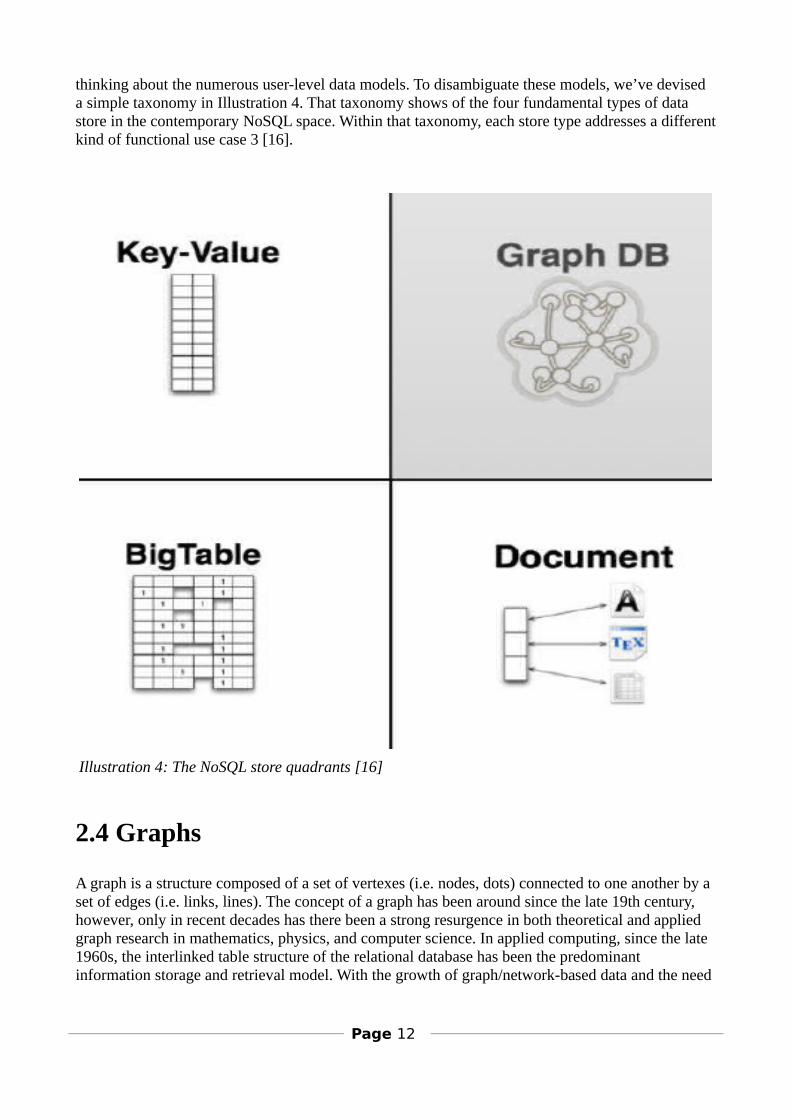
thinking about the numerous user-level data models. To disambiguate these models, we’ve devised a simple taxonomy in Illustration 4. That taxonomy shows of the four fundamental types of data store in the contemporary NoSQL space. Within that taxonomy, each store type addresses a differentkind of functional use case 3 [16].
2.4 Graphs
A graph is a structure composed of a set of vertexes (i.e. nodes, dots) connected to one another by a set of edges (i.e. links, lines). The concept of a graph has been around since the late 19th century, however, only in recent decades has there been a strong resurgence in both theoretical and applied graph research in mathematics, physics, and computer science. In applied computing, since the late 1960s, the interlinked table structure of the relational database has been the predominant information storage and retrieval model. With the growth of graph/network-based data and the need
Page 12
Illustration 4: The NoSQL store quadrants [16]
to efficiently process such data, new data management systems [13] have been developed. In contrast to the index-intensive, set-theoretic operations of relational databases, graph databases make use of index-free, local traversals. This article discusses the graph traversal pattern and its use in computing. Let's begin for the definition of a graph: G = (V, E). This definition states that a graphis composed of a set of vertexes V and a set of edges E. Normally following this definition is the definition of the set E. For directed graphs, E (V × V ) and for undirected graphs, E {V × V }. ⊆ ⊆That is, E is a subset of all ordered or unordered permutations of V element pairings. From a purely theoretical standpoint, such definitions are usually sufficient for deriving theorems. However, in applied research, where the graph is required to be embedded in reality, this definition says little about a graph’s realization. The structure a graph takes in the real-world determines the efficiency of the operations that are applied to it. It is exactly those efficient graph operations that yield an unconventional problem-solving style [13].
Graphs are a flexible modeling construct that can be used to model a domain and the indexes that partition that domain into an efficient, searchable space. When the relations between the objects of the domain are seen as vertex partitions, then a graph is simply an index that relates vertexes to vertexes by edges. The way in which these vertexes relate to each other determines which graph traversals are most efficient to execute and which problems can be solved by the graph data structure. Graph databases and the graph traversal pattern do not require a global analysis of data. For many problems, only local subsets of the graph need to be traversed to yield a solution. By structuring the graph in such a way as to minimize traversal steps, limit the use of external indexes, and reduce the number of set-based operations, modelers gain great efficiency that is difficult to accomplish with other data management solutions.
2.5 Omics and graph databasesThe purpose of this work is to join the omic data (variants in samples) with a graph database. We choose two project as examples or reference of omic data integration in graph databases:
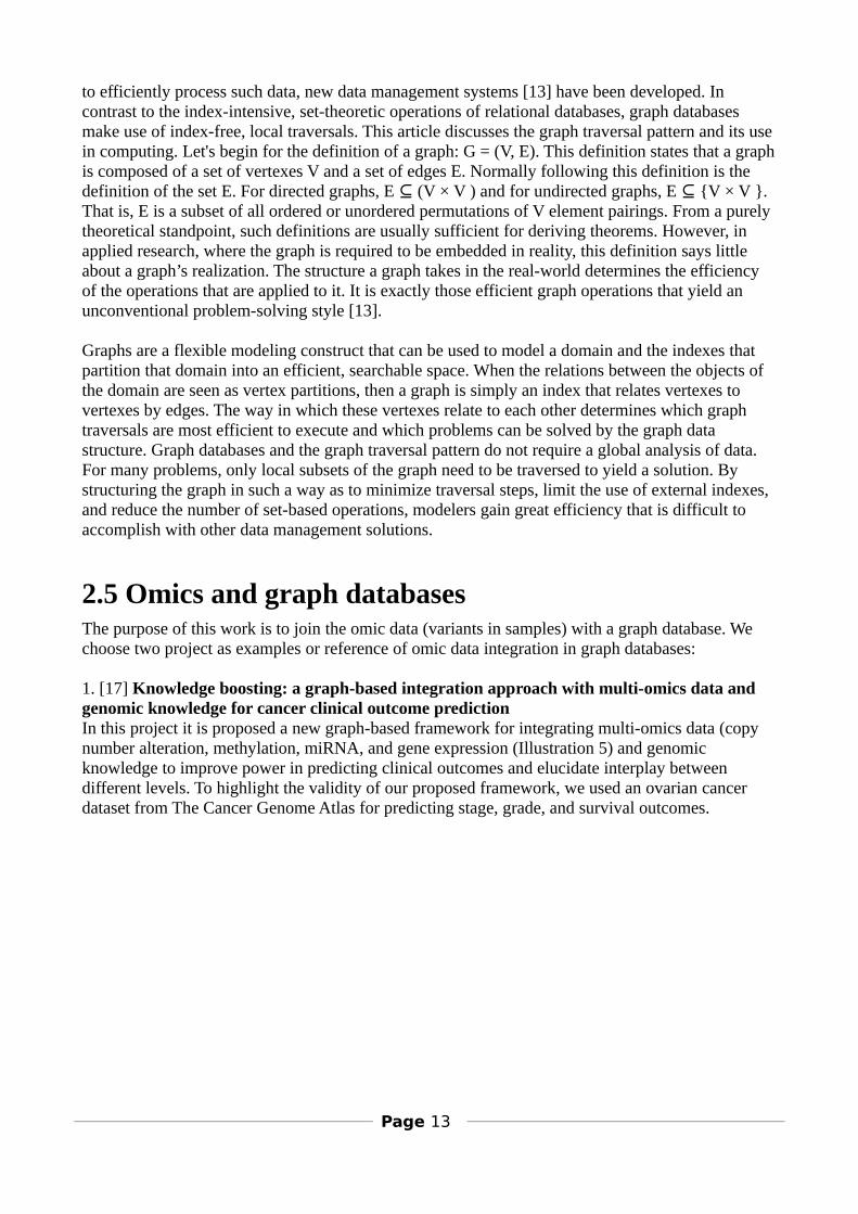
1. [17] Knowledge boosting: a graph-based integration approach with multi-omics data and genomic knowledge for cancer clinical outcome predictionIn this project it is proposed a new graph-based framework for integrating multi-omics data (copy number alteration, methylation, miRNA, and gene expression (Illustration 5) and genomic knowledge to improve power in predicting clinical outcomes and elucidate interplay between different levels. To highlight the validity of our proposed framework, we used an ovarian cancer dataset from The Cancer Genome Atlas for predicting stage, grade, and survival outcomes.
Page 13
2. [18] Multi-omic network signatures of diseaseTo better understand dynamic disease processes, integrated multi-omic methods are needed, yet comparing different types of omic data remains difficult. Integrative solutions benefit experimental researchers by eliminating potential biases that come with single omic analysis. It is been developedthe methods needed to explore whether a relationship exists between co-expression network modelsbuilt from transcriptomic and proteomic data types, and whether this relationship can be used to improve the disease signature discovery process. A naïve, correlation based method is utilized for comparison. Using publicly available infectious disease time series data, it has been analyzed the related co-expression structure of the transcriptome and proteome in response to SARS-CoV infection in mice. Transcript and peptide expression data was filtered using quality scores and subset by taking the intersection on mapped Entrez IDs. Using this data set, independent co-expression networks were built. The networks were integrated by constructing a bipartite module graph based on module member overlap, module summary correlation, and correlation to phenotypes of interest. Compared to the module level results, the naïve approach is hindered by a lack of correlation across data types, less significant enrichment results, and little functional overlapacross data types. Our module graph approach avoids these problems, resulting in an integrated omic signature of disease progression, which allows prioritization across data types for down-stream experiment planning. Integrated modules exhibited related functional enrichments and could suggest novel interactions in response to infection. These disease and platform-independent methods can be used to realize the full potential of multi-omic network signatures.
Page 14
Illustration 5: Schematic overview of integration with multi-omics data and genomic knowledge
3 Materials and methods
3.1 Source dataThe data used has being obtained within the project Endoscreen (http://www.endoscreen.com) which is a Comunidad de Madrid project focused on the endocrine disorders.We have received 96 variants tables in a tabulator separated format (mut file from here). Each one correspond to the variants of a run in the NGS equipment. The samples come from 48 patients. 2 runs are executed in the Illumina NGS equipment for each sample patient: one with the Nextera chemical and one with the Roche chemical. This is done for comparing purposes.The mut file is the starting point for the Urdimbre application, which is the Java application developed for the internship.
Beside the mut files, other kind of source data is necessary in order to construct the graph database:
- HPOs: It is the ontology of all possible human phenotypes- patient_samples: It relates the patients with the samples- HPO_exoma. It relates each patient with the phenotypes- Genes. It details the information about genes.- Geneset. For each geneset it has detailed info about it and a list of genes inside it.- Batch. It contains a list of several of the above files in order to load all together.
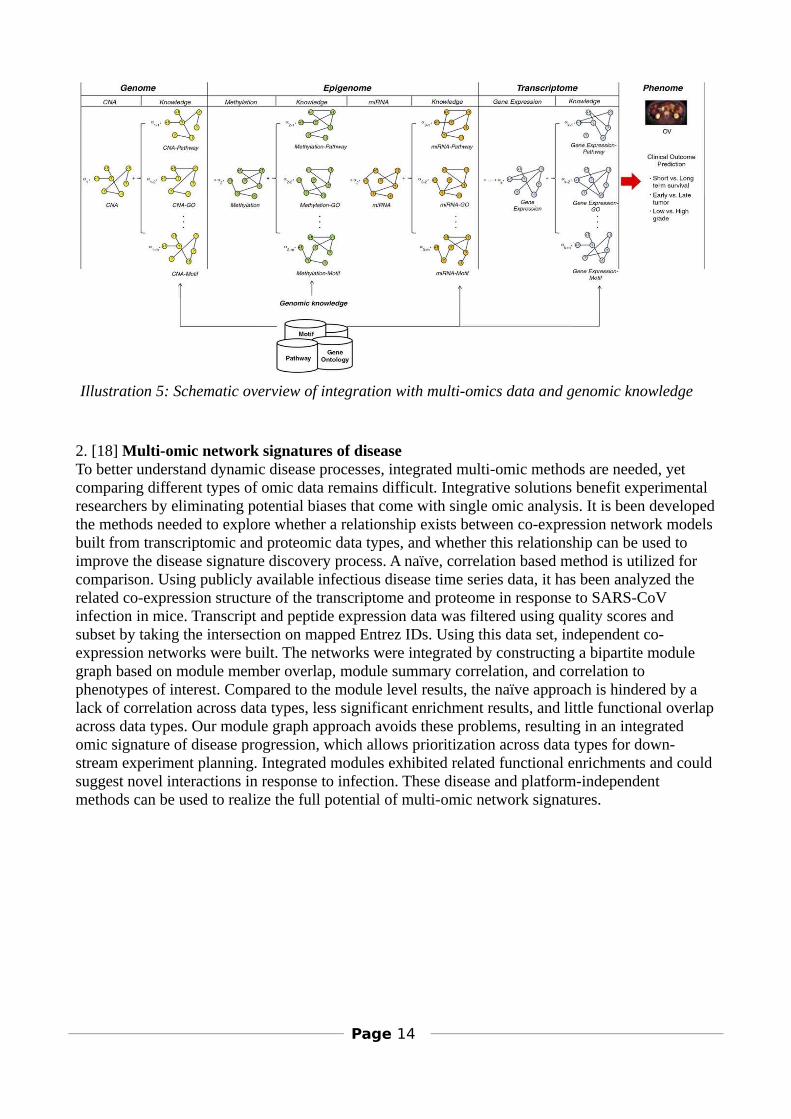
3.2 NGS preliminary analysisThe NGS equipment is a Illumina Myseq [3]. The maximum output given for the equipment is 15Gb. This is an important restriction: we can't analyze the whole genome, just parts of them. The DNA is constrained to exonic regions. This is important because as more regions are captured less samples can be analyzed in the NGS equipment run. Each run takes72 hours and the reagents of each run cost more than 1000 €.In most of molecular tests used in genetics, the interpretable data isgenerated by the same platform where the experiment is done. Andit is only required the technical and the facultative stuff tounderstand the test.Nevertheless, in massive sequencing, data generated are not directlyinterpretable. It's necessary a further analysis for generatingbiologically meaningful data. That analysis is developed by thebioinformatic department. This is the whole process [1]:1. The DNA sample is extracted.2. The DNA is fragmented in smaller pieces for the NGSreading. This is done using a sonication process. 3. The fragments are filtered for just obtaining the library forthe regions we are interested on.4. Adapters with index information are added to the fragmentsof different samples.5. All the samples are joined and put in the NGS equipment with the reagents.6. Inside the Miseq an image is generated for each nucleotide layer pass. The images comprise the raw data generated by the biological process. The images are interpreted and each fragment
Page 15
Illustration 6: Illumina Myseq hybridation method
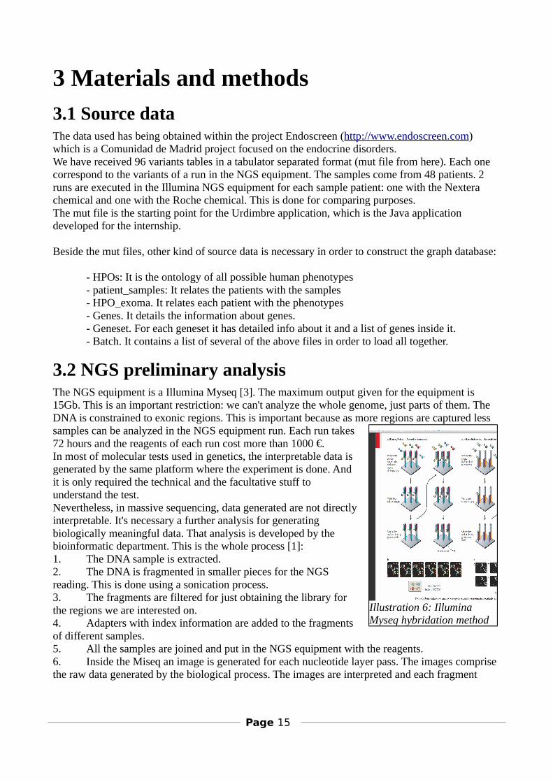
sequence is obtained.
7. Each fragment is sequenced in the NGS equipment like a 'read'. Here, a FASTQ [4] file is generated. The reads have a fixed size of 150 nucleotides.8. Here the bioinformatic process begins. The FASTQ file is subjected to a quality control process to check if the reads are acceptable or not: reads length, coverage, quality of the nucleotidesin the read. FASTQC program [5] is used for accomplishing this control processes.9. From FASTQC the bioinformatic pipeline begins: preprocess, alignment and variant calling and variant filtering are done.
All the mutation data is based on the hg19 assembly.
3.3 General description
The system consists of the following parts:- HBASE is a NoSQL database (key-value) that uses HADOOP. It offers to have the database distributed in several machines. Due to the computer science culture of the staff in bioinfomatic department in La Paz Hospital, we chose this scenario more related to HADOOP because they have in their mind to use clustering systems with redundancy and easy to scale.- ElasticSearch as the indexation engine. It is used by Titan for generating the indexes.- Titan: graph database wrapper that can use several database system under it: Cassandra, Berkeley DB, 'in memory' database, HBASE. Now we are using HBASE.- Urdimbre: Java application developed for the INGEMM which mines Titan resources in order to access to the graph information. It is the only software developed for the internship. The rest is third-party software.
Page 16
Illustration 7: Illumina myseq NGS equipment
3.3.1 HADOOPApache Hadoop is an open-source software framework for storage and large-scale processing of data-sets on clusters of commodity hardware. Hadoop is an Apache top-level project being built andused by a global community of contributors and users. It is licensed under the Apache License 2.0 [30].The Apache Hadoop framework is composed of the following modules:- Hadoop Common: contains libraries and utilities needed by other Hadoop modules.- Hadoop Distributed File System (HDFS): a distributed file-system that stores data on commodity machines, providing very high aggregate bandwidth across the cluster.- Hadoop YARN: a resource-management platform responsible for managing compute resources in clusters and using them for scheduling of users' applications.- Hadoop MapReduce: a programming model for large scale data processing.
All the modules in Hadoop are designed with a fundamental assumption that hardware failures (of individual machines or racks of machines) are common and thus should be automatically handled insoftware by the framework. Apache Hadoop's MapReduce and HDFS components originally derived respectively from Google's MapReduce and Google File System (GFS) papers [30].
3.3.2 HBASEHBase is an open source, non-relational, distributed database modeled after Google's BigTable and written in Java. It is developed as part of Apache Software Foundation's Apache Hadoop project andruns on top of HDFS (Hadoop Distributed Filesystem), providing BigTable-like capabilities for Hadoop. That is, it provides a fault-tolerant way of storing large quantities of sparse data (small amounts of information caught within a large collection of empty or unimportant data, such as finding the 50 largest items in a group of 2 billion records, or finding the non-zero items representing less than 0.1% of a huge collection) [29].
3.3.3 ElasticSearchElasticSearch is a search server based on Lucene. It provides a distributed, multitenant-capable full-text search engine with a RESTful web interface and schema-free JSON documents. Elasticsearch isdeveloped in Java and is released as open source under the terms of the Apache License.[28]
ElasticSearch can be used to search all kinds of documents. It provides scalable search, has near real-time search, and supports multitenancy [4]. ElasticSearch is distributed, which means that indexes can be divided into shards and each shard can have zero or more replicas. Each node hosts one or more shards, and acts as a coordinator to delegate operations to the correct shard(s). Rebalancing and routing are done automatically [28]
3.3.4 TitanTitan is a scalable graph database optimized for storing and querying graphs containing hundreds ofbillions of vertexes and edges distributed across a multi-machine cluster. Titan is a transactional database that can support thousands of concurrent users executing complex graph traversals in real time [26].
In addition, Titan provides the following features:
Page 17
Elastic and linear scalability for a growing data and user base. Data distribution and replication for performance and fault tolerance. Multi-datacenter high availability and hot backups. Support for ACID and eventual consistency. Support for various storage backends:
Apache Cassandra Apache HBase Oracle BerkeleyDB
Support for global graph data analytics, reporting, and ETL through Apache Hadoop integration.
Support for geo, numeric range, and full-text search via: ElasticSearch Apache Lucene
Native integration with the TinkerPop graph stack: Gremlin graph query language Frames object-to-graph mapper Rexster graph server Blueprints standard graph API
Open source with the liberal Apache 2 license.
3.3.4.1 Gremlin
Gremlin is a the graph traversal language used by Titan. Gremlin works over those graph databases/frameworks that implement the Blueprints property graph data model. Gremlin is a style of graph traversal that can be used in various JVM languages. The specific distribution of Gremlin provides support for Java and Groovy [27].
3.3.5 Urdimbre structureIt is the Java application that has been developed for the internship. It uses Titan for accessing to thegraph information.
It is composed by three Java packages:- INGEMM.graph. (24 class files and 3144 source code lines) It contains the main function, the graph API itself, the abstract classes for graph visualization and access to the DB. Also contains the window system- INGEMM.jung (3 class files and 356 source code lines) contains the concrete classes for graph visualization with the Jung [31] library.- INGEMM.titan (16 class files and 1410 source code lines, including OTF (OnTheFly) example files) contains the concrete classes for the access to DB with Titan [26].
Both last packets are replaceable with other packets that use different libraries if someone wants to use another software.
Page 18
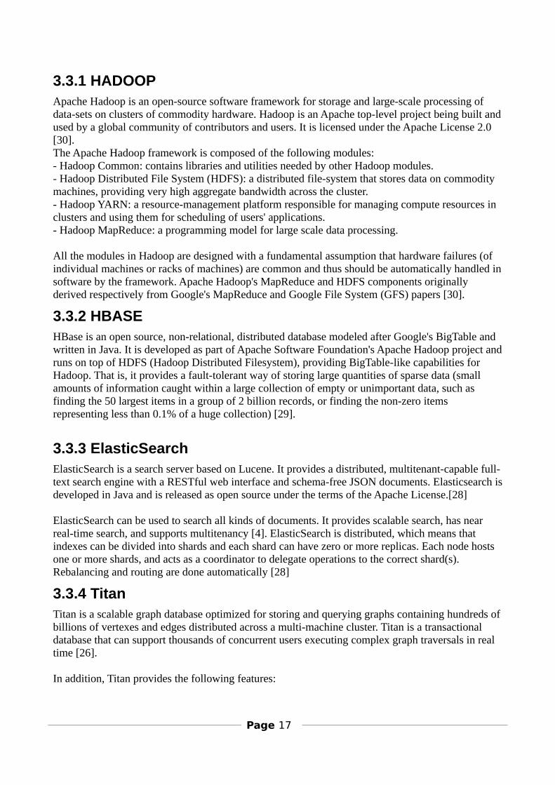
3.3.5.1 On The Fly Remote class creation
We need a very high level of configuration when we load the data and when we create the database. In both cases we have used a system to load classes and execute them after the Java application have been launched.This is useful to do little modifications in these classes. Actually these classes are used like scripts.In this way we can load any kind of file in the database. It is not necessary to recompile the application to be able to load the file.In the title we use the word “remote” because in a client-server scenario we send by sockets the Java class to the server and will be compiled and executed there to load or create the data base.The system is extremely flexible.
3.3.5.2 Graph access API
From the application it is possible to make a query and convert its result in a graph of the Graph class. This graph keeps all vertex and edges that could be examined by means of Node and Connection classes.When data is inserted in the database theses classes will be in charge of test the restrictions. The restrictions will be in the properties _restrictions and _required of GraphElement. In _restrictions will be stored regular expressions that the property must comply when is inserted in the graph element. In _required will be the properties that are mandatory when a commit of the GraphElementis done.Both kinds of restrictions will be introduced in the specific class constructors. In this example we are going to force to genotype property to be like “two digits separated by a slash” and we will force to the mutation to have an “alt” property.
Page 19
Illustration 8: On The Fly loading system

public Mutation(String name){
super( "mutation", name);this._prefix = "m_";
this._restrictions.put("genotype", "\\d/\\d");this._required.add("alt");
}
Page 20
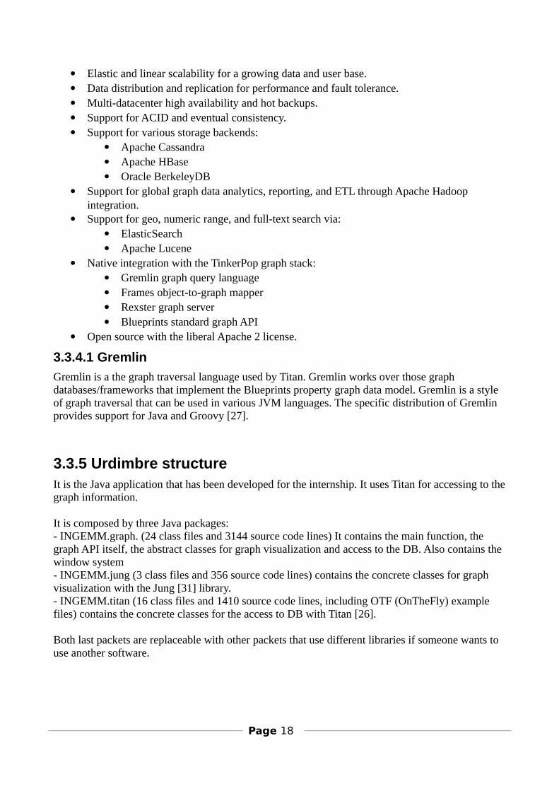
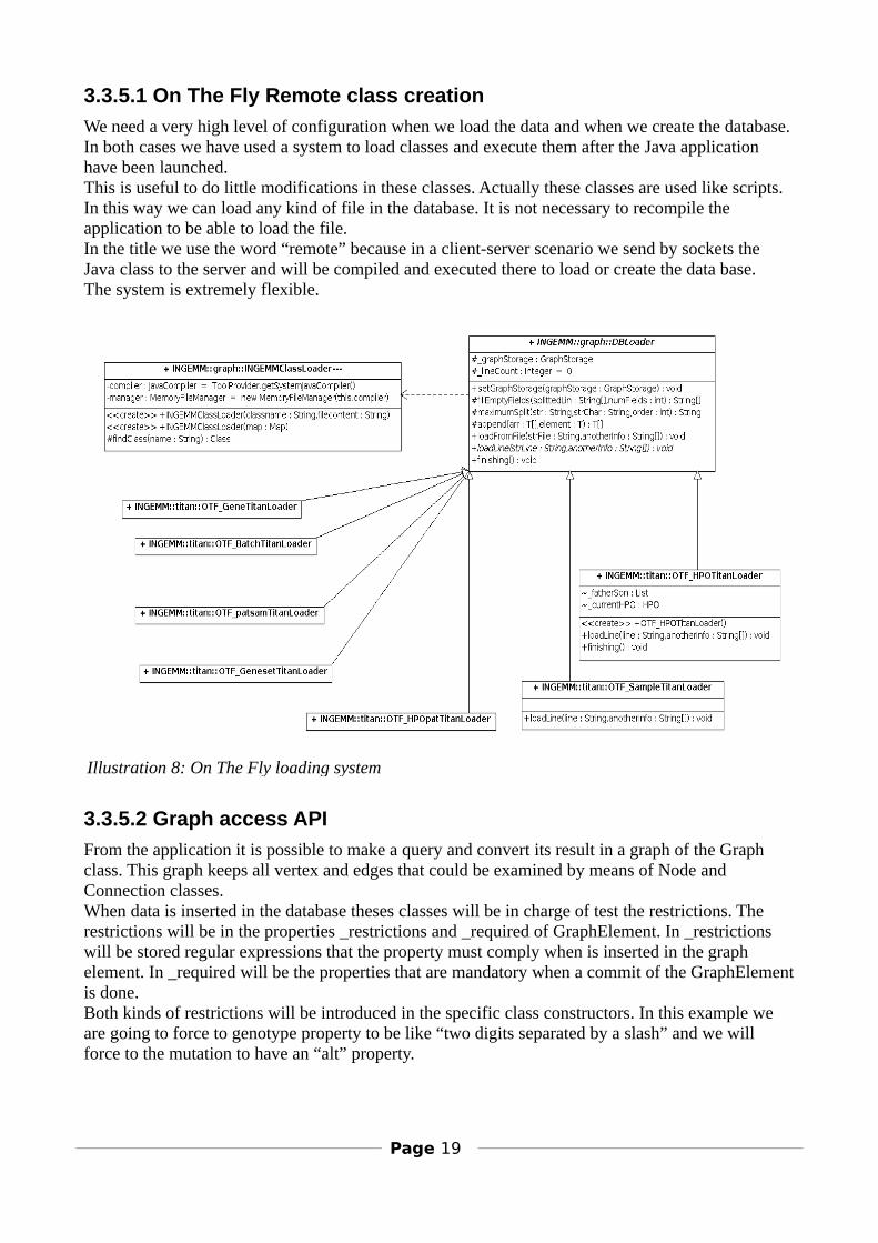
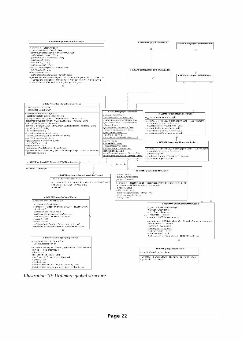
3.3.5.3 Urdimbre general structure
In this picture we can see the general operation of Urdimbre. In the middle is shown the Urdimbre class, which is the launcher of the rest of components:- GraphStorage is the abstract class from where the concrete DB access class inherits (GraphStorageTitan, for example).- GraphDBLoader is the base class of all the On The Fly loaders.- MouseController is the base class for the concrete jungMouseController.- SocketLookAfterThread is the class which is instantiated for each client connected to the server.- GraphViewer is the abstract class for viewing graphs.- INGEMMWindow is the base class for the windows.
Page 21
Illustration 9: Graph and Graph element hierarchy
Page 22
Illustration 10: Urdimbre global structure
4 ResultsFollowing the same structure as proposed in the internship objectives, we separate the results in three phases:
4.1 A: graph databases analysisThere are a many graph database managers / libraries. The most relevant we have seen are: Neo4J, OrientDB, DEX, ArangoDB, Titan, Stinger and the graph part of Boost libraries [33].There are ones with an associated storage system and ones without it. For instance, Stinger is just a graph manager developed in C++ without storage system. The graph is loaded into the memory at the beginning and we operate over it.Some of the databases are completely graph oriented and other are simply NoSQL. For instance, ArangoDB is a key-value type database, more general purpose, but it is possible to use for graphs generating edges as key-value.
There are several query languages for accessing to the graph information: cypher (Neo4J), Gremlin,SPARQL, AQL (ArangoDB). This is because the way we query a graph database is different from a relational database.
4.1.1 ApproachesSome different database software was checked in order to select the most suitable for the project:
We began trying the Neo4j graph database [33] because is the most popular. It is just for graphs. It is developed in Java and it has a big community behind and many associated tools easily installable. In the tests it causes many performance problems, mainly in the vertex andedge insertion. Other important drawback is that there are several versions of licenses and only the “community version” is free (http://www.neo4j.org/download).The checked version was the community one. We check the py2neo API [41] for Python andwe found many bugs. The documentation is deficient and many important functions are not commented. In addition to this we have doubts about the scalability of the system. This is very important for using because it will have to be scaled to the INGEMM big amount of data.
Another tested database software is ArangoDB [42]. It is developed in C++ (interesting for good performance). It is NoSQL, including paradigms: documents, key-value and graphs. The API looks not very polished. The quickstart example was difficult to start running. It was necessary to change some pieces of source code. There is a lack of documentation. We think it was so risky to use it.
DEX [43]. It was discarded because it has a big limitation of 1.000.000 vertexes. Stinger [44] and Boost [45] are C++ libraries. They hasn't own storage system and it forces
to maintain the whole graph in memory. It is very efficient, but there is a risk because it needs a big development in C++.If any time there is a performance problem could be a good solution to load the graph in memory with Stinger and do the query from there. Stinger is the most powerful engine for graph traversing, but Gremlin or cypher are not supported.
OrientDB looked a good option, but it was said that it had been overtaken by ArangoDB andwe had already discarded ArangoDB.
Page 23

In graph representation:
We spent much time in checking Cytoscape. It is widely used in system biology and it looked a good idea to use it for represent the results. The graphical representation is very fast and the algorithms to place the vertexes and the edges are good.The problems comes with the integration with Java. You can add your own Java like a plug-in using OSGi. But it was impossible to create the plug-in. There were many dependencies that caused it to fail.
4.1.2 Final technological approachThe way we have implement the system is the following:
- Titan [26] as graph database, with HBASE+HADOOP as its storage system.
- The Java API Jung as the libraries for graph representation.
- A Java application called Urdimbre developed for the INGEMM.
- Blueprints [46] as the libraries to make queries programatically.
- Gremlin [27] as graph query language.
Page 24
Illustration 11: Component diagram

4.2 B: Implementation of the database and the database scheme
Although one of the paradigms of the graph databases is that the schemes doesn't exists or they are very easy to change, we have developed a scheme of which is the aspect of the graph. Indeed it is more a graphical representation than a real software restriction.The graph database scheme is the result as biological issues as clinical and bioinformatic issues. In some places, for performance reasons, some data have been duplicated.
For the moment we are going to use variants found in the NGS analysis. We are not going to use multi-omics as in other approaches.
As important issues, we can highlight:- The patient can have several episodes in the time. In each episode a sample can be taken. Maybe itis interesting to compare the variants between different episodes. This would be more for somatic mutations.- In many nodes (locus, mutation, gene) we have the start and end properties. These are very important for us because they permit us to query the location of the entity.
Page 25
Illustration 12: Graph database scheme for the INGEMM data
- Many queries are done by means of the properties: name, type, start and end. This is the reason because for the moment these are the indexes for our database. These properties use to be the starting point for the queries, and then it is important that this first search will be fast.- An entity called MutationInSample is created because there are details in the particular variant in asample that can't be contained in the Mutation, for example the genotype.- It is very interesting to add interaction networks: protein, metabolites … In this way we can relate variants between them, and we can obtain extra information about how they work over the phenotype.- There are parent-child relations between patients. In this way we can find some data by making joined queries with them.- The chromosome is considered as a vertex and not as a property because it contains characteristic information. If it was a property in a node: what type of node would contains this property?: gene, mutation, locus, … we think it is more convenient to exist as a vertex and the vertex interested in the chromosome information will establish an edge with it.Other plus is that if we want to look for something inside the chromosome, it is fast to find the edges connected with it. In the other way we'd have to look for in the chromosome property of all the nodes.- Some values, as the distance between a locus and the nearest gene, are written in the edge that connects the locus and the gene. This is done in this way because the distance is not a characteristic of none of the vertex, but of the relationship between them. In the distance case could occur that onelocus was related with different genes: the distance between all of them will be different.- Light entities, as the band belonging to a chromosome, that are not schedule to use as the central axis of any query, are modeled as properties of another vertex (the locus in this case). We know that the band is analogue to a chromosome (both are regions into the genome), but because of the way the INGEMM use the information we consider not to use a vertex in this case.- The databases where the mutations are documented are properties of the mutation.- The vertex locus is important for us. This is because over the same locus is possible to find severalmutations (different nucleotide changes). This is because several mutations are connected with one locus.- The great majority of properties are strings. There are some exceptions. The most important are the properties start and end. Both of them are numerical. This is very important because when we find ranges in genome regions is faster to compare numbers than convert string to numbers and compare then.- The entity transcript is not included for the moment in the model. In some approaches was between the locus and the gene. But for the current queries we don't need it and it makes the graph much more complex. Maybe for further uses.
4.2.1 Urdimbre user graphic interfaceThis is a brief Urdimbre user interface description:
Page 26
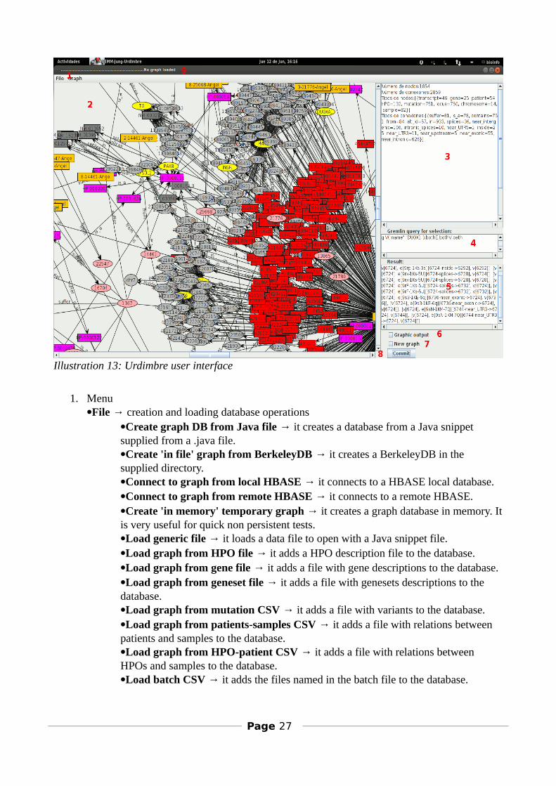
1. MenuFile → creation and loading database operations
Create graph DB from Java file → it creates a database from a Java snippet supplied from a .java file.Create 'in file' graph from BerkeleyDB → it creates a BerkeleyDB in the supplied directory.Connect to graph from local HBASE → it connects to a HBASE local database.Connect to graph from remote HBASE → it connects to a remote HBASE.Create 'in memory' temporary graph → it creates a graph database in memory. Itis very useful for quick non persistent tests.Load generic file → it loads a data file to open with a Java snippet file.Load graph from HPO file → it adds a HPO description file to the database.Load graph from gene file → it adds a file with gene descriptions to the database.Load graph from geneset file → it adds a file with genesets descriptions to the database.Load graph from mutation CSV → it adds a file with variants to the database.Load graph from patients-samples CSV → it adds a file with relations between patients and samples to the database.Load graph from HPO-patient CSV → it adds a file with relations between HPOs and samples to the database.Load batch CSV → it adds the files named in the batch file to the database.
Page 27
Illustration 13: Urdimbre user interface
Graph → information about the current database / graphView current graph → it shows the whole graph contained in the database. It can be very slow.Get database statistics → it shows in zone 3 of Illustration 11 a summary of the current database.Delete the whole database → it deletes completely the database.
2. Panel where the graph is shown. Inside it it is possible to shift, make vertex selection and make zoom with the mouse wheel. It permits to move nodes. The layout currently used in the panel is FRLayout [47] (Jung libraries) and it will try in 50 iterations to place the nodes in the best way in order to interpret the graph.
3. Textbox where the general and progress information are shown.4. Textbox to write queries.
In multi-sentence queries, they will be separated by semicolon. In multi-sentence queries where there is a pipeline with postprocess required it must
be forced. Example: Generate a table with the columns: chromosome node and chromosome
name. In the gremlin console, the query would be:gremlin> t = new Table()gremlin> g.V("type","chromosome").as('x').name.as('y').table(t)gremlin> t
In this box it should be:t = new Table(); g.V("type","chromosome").as('x').name.as('y').table(t).iterate(); t
5. Here the query result is shown.6. Checkbox where we specify if we want to see the result in a the graphical panel (2).
We have to take into account that if the result of the query is a big amount of vertexes and edges it will take a lot of time to show it.
It is important too to to notice that sometimes the result is not a graph, but a number, for example. Then it will be just shown in the zone 5.
If we want to force that all the steps and all the connections in the pipe will show in the graph we must to add .path at the query and specify the output and input of each vertex and edge. Example: “Give me all the nodes connected to the gene DUOX1 at a distance of 2 or less”:Instead of g.V("name","DUOX1").both.both It gives just the vertexes at a distance of exactly two edges and just the vertexes, not the edges. The way for watching the graph is: g.V("name","DUOX1").bothE.bothV.bothE.bothV.path
7. If we want that the graphical result will generate a new graph we must to check this checkbox. If not the currently shown graph just will be highlighted with the query result.
8. Button for sending the query to the database.9. Window caption where is shown the database type attacked by Urdimbre.
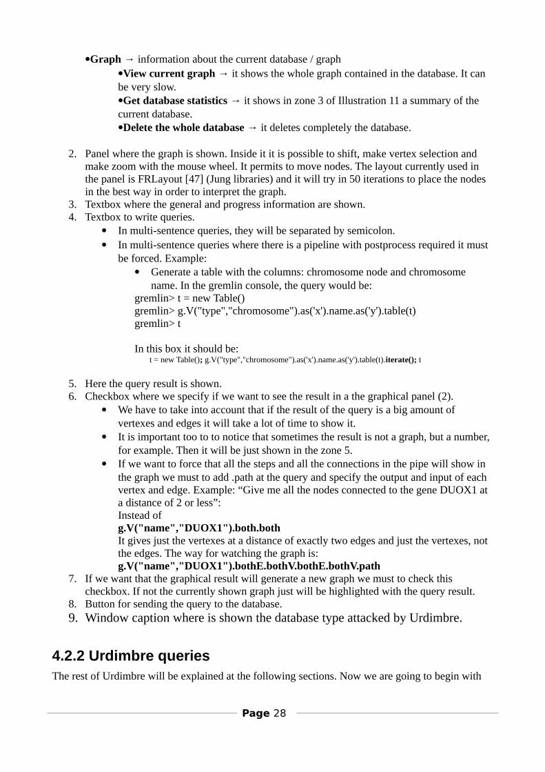
4.2.2 Urdimbre queriesThe rest of Urdimbre will be explained at the following sections. Now we are going to begin with
Page 28
some simple queries that helps to understand better how Gremlin queries works:
- All the nodes related directly to the gen DUOX1:g.V("name","DUOX1").bothE.bothV.path
If you click with the mouse over the “DUOX1” vertex you will obtain the following information:
*** gene: DUOX1DBId: 67028accesionNumbers: AF213465CCDSID: CCDS32221.1OMIMID: 606758PubmedID: 10806195GeneFamilyTag: EFHANDstatus: ApprovedlocusType: gene with protein productsynonyms: NOXEF1, THOX1, LNOX1ApprovedName: dual oxidase 1approvedDate: 2000-05-30RefSeqID: NM_017434modifiedDate: 2013-01-10
Some simple queries to test the data are well read:
- How many samples do we have?:
Page 29
Illustration 14: Graphic result of "g.V("name","DUOX1").bothE.bothV.path"
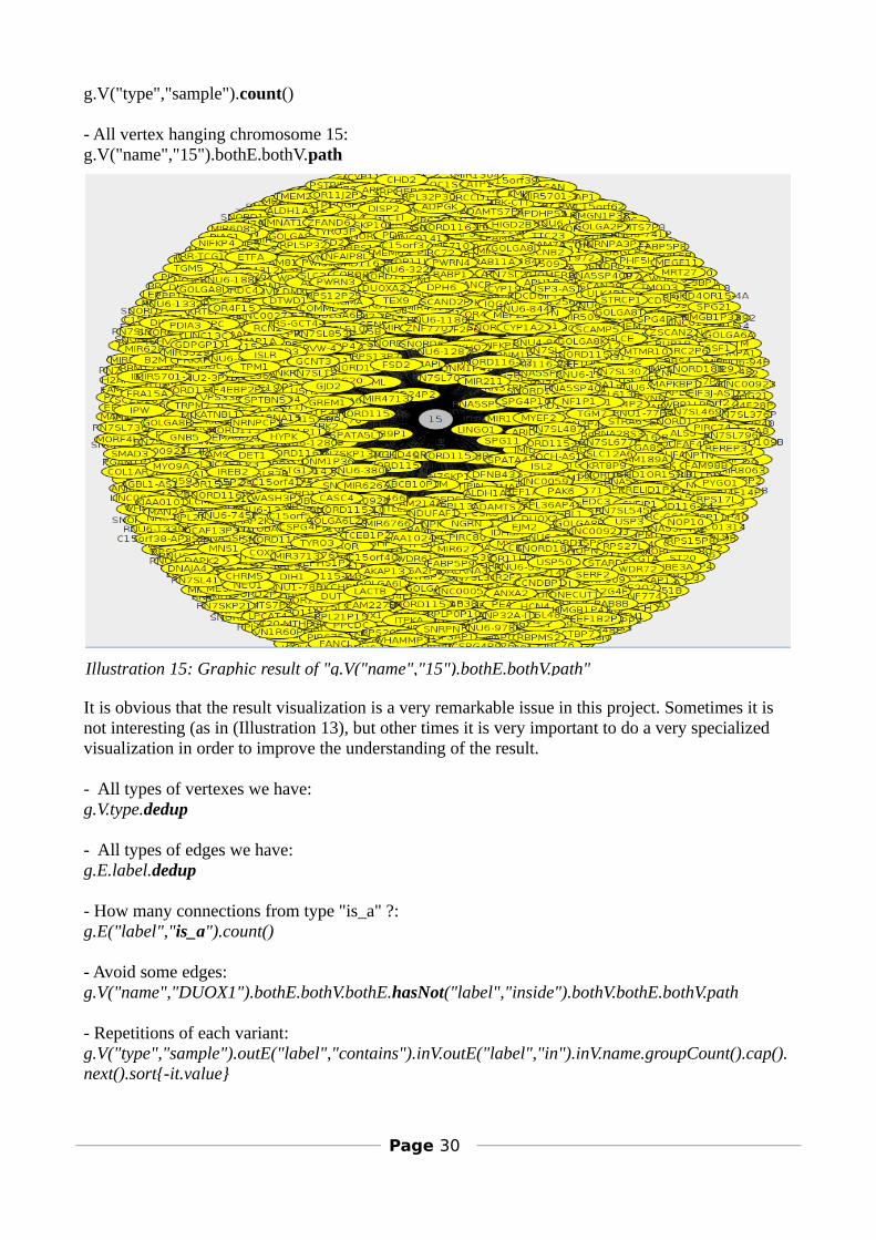
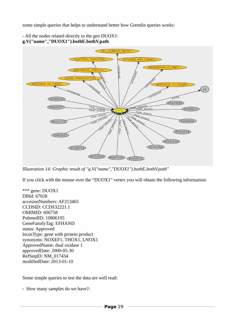
g.V("type","sample").count()
- All vertex hanging chromosome 15:g.V("name","15").bothE.bothV.path
It is obvious that the result visualization is a very remarkable issue in this project. Sometimes it is not interesting (as in (Illustration 13), but other times it is very important to do a very specialized visualization in order to improve the understanding of the result.
- All types of vertexes we have:g.V.type.dedup
- All types of edges we have:g.E.label.dedup
- How many connections from type "is_a" ?:g.E("label","is_a").count()
- Avoid some edges: g.V("name","DUOX1").bothE.bothV.bothE.hasNot("label","inside").bothV.bothE.bothV.path
- Repetitions of each variant: g.V("type","sample").outE("label","contains").inV.outE("label","in").inV.name.groupCount().cap().next().sort{-it.value}
Page 30
Illustration 15: Graphic result of "g.V("name","15").bothE.bothV.path"
- Test if there are any repeated mutation g.V("type","sample").outE("contains").inV.groupCount().cap().next().sort{-it.value}
- Most repeated mutation in the HPO 'HP:0004904': g.V("name","HP:0004904").inE("suffer").outV.inE("from").outV.outE("contains").inV.outE("case_of").inV.groupCount().cap().next().sort{-it.value}
- Show in tree style from 'DOUX1': g.V("name","DUOX1").both.out.tree.cap
- Chromosomes sorted by the number of genes contained: g.V("type","gene").outE("inside").inV.name.groupCount().cap().next().sort{-it.value}
- HPOs associated to any patient:g.V("type","HPO").inE('suffer').back(2).name
- Loci inside the range:1500000-1505000:g.V("type","locus").interval("start", 17450000, 17460000)
- Delete all the database:g.V.remove(); g.E.remove()
- Vertexes with less than two connections:g.V.filter{it.bothE.count() < 2}.path
4.2.3 Specific hardware infrastructureIt is specified the infrastructure used in the final test: in the server side and in the client side.
4.2.3.1 Server side
To assert transparency of graph database design from underlying storage and system scalability, a single node deployment and a distributed one was tested. For distributed environment testing a HBASE over a 5 node Hadoop cluster was configured. Due to limitations on hardware available follow Hadoop best practices for hardware selection was impossible and many requirement amount of RAM on Name Nodes, virtualization of nodes or underlying filesystem and partitioning for data nodes containing data blocks of Hadoop Distributed Filesystem- were relaxed.
Hadoop-2.2.0 cluster:
Name Node:
Debian GNU/Linux 7 (wheezy) x64 virtualized with XenServer 6.2
244 Mb RAM
1 vCPU Intel(R) Core(TM) i3-2100 CPU @ 3.10GHz
7.3 Gb HDD.
Resource Manager & Secondary Node Name:
Page 31
Debian GNU/Linux 7 (wheezy) x64 virtualized with XenServer 6.2
244 Mb RAM
1 vCPU Intel(R) Core(TM) i3-2100 CPU @ 3.10GHz
7.3 Gb HDD.
3 x Data Nodes + Node Manager:
Debian GNU/Linux 7 (wheezy) x64
32 Gb RAM
Intel(R) Xeon(R) CPU E5-2620 0 @ 2.00GHz
1000 Gb ZFS filesystem from Raidz2 zpool for HDFS blocks.
Hbase-0.94.20
Master Node:
Debian GNU/Linux 7 (wheezy) x64 virtualized with XenServer 6.2
244 Mb RAM
1 vCPU Intel(R) Core(TM) i3-2100 CPU @ 3.10GHz 7.4 Gb HDD.
3 x Regional Server:
Debian GNU/Linux 7 (wheezy) x64
32 Gb RAM
Intel(R) Xeon(R) CPU E5-2620 0 @ 2.00GHz
1000 Gb ZFS filesystem from Raidz2 zpool for HDFS blocks.
Zookeeper 3.4.6:
Every single node of cluster runs a Zookeeper instance.
Java Virtual Machine: Java(TM) SE Runtime Environment (build 1.7.0_55-b13)
4.2.3.2 Client side
We used an Ubuntu 14.04 LTS system running over a Lenovo B590: core i3, RAM 4GBJava Virtual Machine: Java(TM) SE Runtime Environment (build 1.7.0_67-b01)
4.2.4 Specific software infrastructureThe configuration we use for HBASE in HADOOP is: 5 HADOOP nodes: 3 nodes for file system completely symmetric, head node (primary) that is the name server (file names), and the secondary node that is in charge for doing backup in order to help to a service restoring.HBASE has a master node and 3 region server nodes. There are 5 zookeeper instances running in allnodes. The zookeeper keeps which are the HBASE servers that are available for a service.
Page 32
4.2.5 Urdimbre command line descriptionThe application is launched with $ Java -jar Urdimbre.jar options
These are the available options:
-server port. The application is launched in server mode.-client host port. The application is launched in client mode.-d javaFile args. The application is connected to the database by means of the Java file javaFile. Args are optional arguments for the connection.-c command. It executes the command “command”. The command is one of these:
- insert: it inserts new data in database (it requires -i option)- query: it makes a query to the database (it requires -q option)- getInfo: it returns general information about the current database.- getAllGraph: it returns all the vertexes and edges stored in the database.- socketClose: it indicates to the server that the connection have been released.
-i file javaFile anotherInfo, It inserts the file “file” into the database with the script javaFile and the options “anotherInfo”.-q query. It launches the query to the database and receive the response.-h. It gives the help message with the available options.
4.2.6 Urdimbre multiple use casesUrdimbre can be used in four different ways:
Server mode. For example: listening in the port 7000 (sockets communication). It can be closed with a “kill” or with CTRL + C.This mode is useful in combination with another application in client mode. It is interesting to be run in power computers to free this computation load to lighter computers.
$ java -jar urdimbre.jar -server 7000
Client mode (graphic mode). For example: against a server located at ip 192.168.0.3 at port 7000 (sockets communication). If the server is not listening the graphic interface is not opened and a message telling it is shown.This mode is useful in combination with another application in server mode. It is useful for light computers that are just going to show the result of the queries or to send orders.
$ java -jar urdimbre.jar -client 192.168.0.3 7000
Standalone mode. Being its server itself. It finishes when the application client window is closed.This mode is interesting to make quick tests. This is because is a standalone and self-contained mode.
$ java -jar urdimbre.jar
Command line mode. For example: connects to the HBASE database defined in the Java fileand inserts in it a list of files defined in batchPeq.csv. When this is done the program exits.
Page 33
If we don't need graph visualization this is the better mode: quicker and easier to redirect results to a text file.
$ java -jar urdimbre.jar -d "/home/.../OTF_inmemoryTitanCreator.java" -c insert -i "/home/.../OTF_BatchTitanLoader.java " "/home/.../batchPeq.csv"
All the communication between client and server are done by means of socket and ASCII code. Themessages sent from client to server are the same as the arguments in the command line.In addition to this arguments/commands are sent, the rest of information needed to complete the request or the response are sent by the socket. For example, if in the request any file is involved, it is sent by the socket. The responses are completely sent by the socket too.
4.2.7 Urdimbre loadingUrdimbre loads the graph database in an incremental way. We can load one file in a session and then another file later and both files generates different graph that are combined.
It is very important to pay attention to the fact that our database is not going to suffer frequent changes. This is because the database is changed just when some new samples need to be loaded or a new property is added. But it is not a database constantly suffering updates. It is more common that big amount of new data is inserted into the database. We try to take advantage of this fact by using the concept of batch loading (later explained).
Because the type of files can be used for load the graph database can be very varied, we have develop a very flexible method to load the files into the database.The pieces of code in charge of loading are scripts of Java that are loaded under demand in the application. They can be written and executed while the application is running.In this way is very quick and easy to build or change a loader. The only necessary thing is to derive from DBLoader class.
The process in the application is the following:1. The user specifies the file to load and the Java file in charge of loading.2. If the application is in client-server mode the file to load and the Java file are sent to the server bysockets.3. In the server side the Java class inside the Java file is instantiated.4. The file is opened and passed to the recently created loader class5. The graph is built and stored.
The politics about how the graph grows is decided inside each loading Java module. It means that there will be the following node insertion cases:- When we try to insert a node we look for a node with the same id. If it exists, then the new node isnot inserted.- We always insert nodes.- If a node with the same id is found then the node is updated.Depending on the Java loading module we use, we can use one ore another politic.
In the INGEMM environment is usual to receive several sample files. For this reason a batch loading method has been created. In a batch loading procedure we open a transaction and don't commit it until all the data is loaded. This is a big increasing in the performance. If we do a commit
Page 34
for every vertex or edge we add, the loading would be incredibly slow. The transaction also provides coherence (all the graph nodes and arcs, or none of them) in case of failure.
This system consists of a .csv file with the following features:1. Each line correspond to a new file to load. Each line has at least two fields: the file to load and the Java file responsible of the loading.2. Each line can specify more of two fields depending on the needs of the Java loader.3. Blank lines are permitted (for separation purposes).4. It is possible to specify string substitutes. The substitutes must be declared at the beginning of thefile. Mainly for avoid big string repetitions. An example:
$1=/home/bioinfo/INGEMM/urdimbre/urdimbre/src/INGEMM/titan$4=/home/bioinfo/INGEMM/urdimbre/urdimbre/data$1/OTF_HPOTitanLoader.java,$4/hpMini.obo
4.2.8 Urdimbre database creation
At the beginning none database exists. It means that the first step is to create a database where we will store the vertex and the edges.At this step we are going to specify:- The kind of storage backend: Berkeley, Cassandra, 'in memory', HBASE.- The parameterization of the storage backend: indexation engine, host name and ports, tables name,storing directories, if write operations are supported, if batch-loading is supported, buffer sizes, username, password.- The indexes of the database.
Because the combination of database creation is huge, we use a scripting system to create or connect to a database. As in the previous point we will use the Java reflection system. On the fly wespecify a Java file which will be in charge of create or connect to the database. In this file all the creation details previously commented will be specified.
4.2.9 Starting from scratch with INGEMM informationFirst of all we launch HBASE in the server side by means of:$ ./bin/start-hbase.shWe launch the indexing engine with:$ bin/elasticsearch -fWe launch Urdimbre in server mode:$ Java -jar urdimbre.jar -server 7000
Now we have the server side ready but we have still not created a specific database.
From the client side we launch:$ Java -jar urdimbre.jar -client bioinfo01-ingemm 7000From the menu we select “File / Connect to graph from local HBASE”. With this operation the Javafile OTF_LocalHBASETitanCreator.java on the fly will be executed:
Page 35
public TitanGraph create(){
BaseConfiguration config = new BaseConfiguration(); Configuration storage = config.subset(GraphDatabaseConfiguration.STORAGE_NAMESPACE);
storage.setProperty("backend","hbase"); storage.setProperty("hostname","bioinfo02-ingemm:2181,bioinfo01-ingemm:2181,hd02-ingemm:2181,hd01-ingemm:2181,bioinfo03-
ingemm:2181"); storage.setProperty("tablename","urdimbre");
storage.setProperty("index.search.backend","elasticsearch"); storage.setProperty("index.search.hostname","bioinfo01-ingemm"); storage.setProperty("index.search.client-only",true); storage.setProperty("index.search.local-mode", true);
TitanGraph titanGraph = TitanFactory.open(config);
// If the indexes are created, an exception is launched and captured with an informative message try {
titanGraph.makeKey("name").dataType(String.class).indexed(Vertex.class).make(); titanGraph.makeKey("type").dataType(String.class).indexed(Vertex.class).make(); titanGraph.makeKey("start").dataType(Integer.class).indexed(Vertex.class).make(); titanGraph.makeKey("finish").dataType(Integer.class).indexed(Vertex.class).make();
titanGraph.commit(); } catch (IllegalArgumentException e1) {
Window.output("The HBASE database was already created. It is just opened"); } return titanGraph;
}
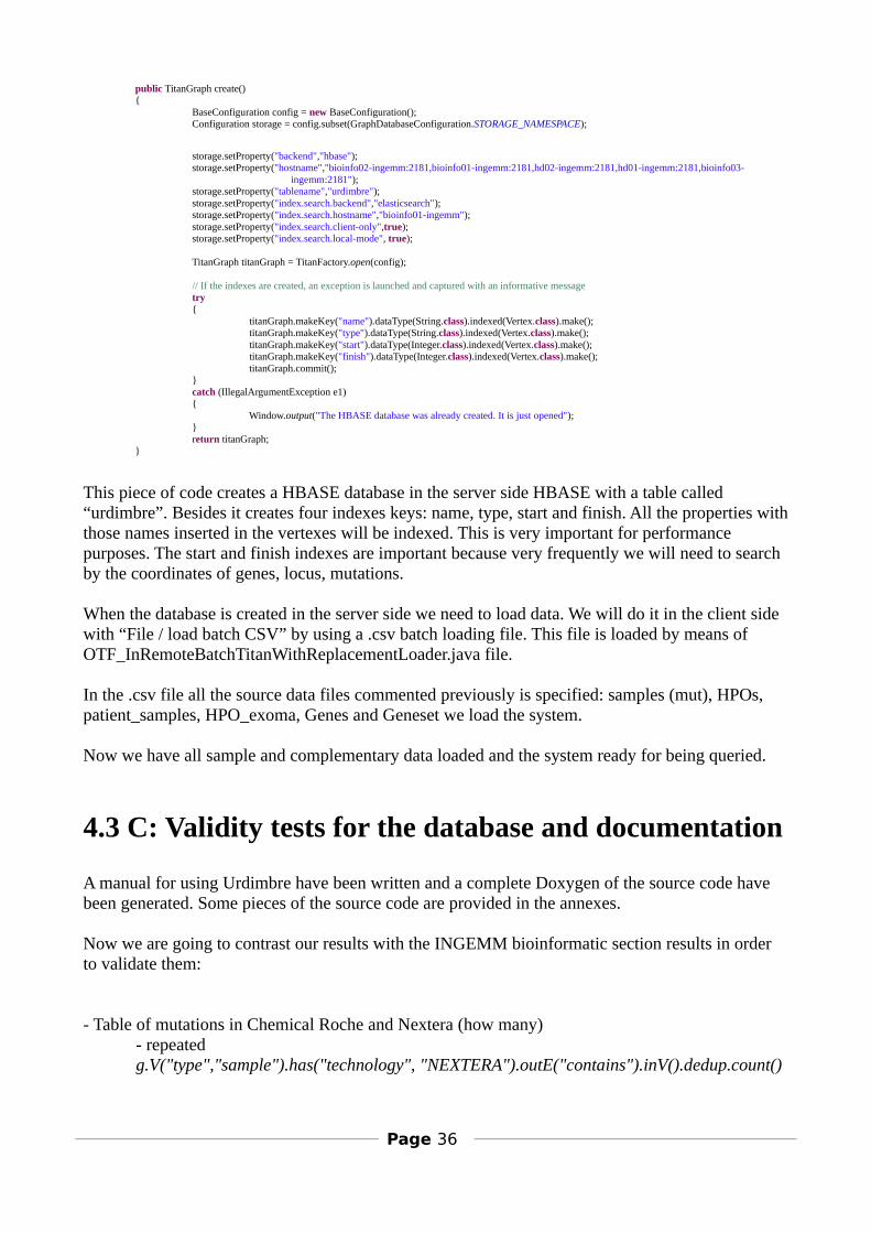
This piece of code creates a HBASE database in the server side HBASE with a table called “urdimbre”. Besides it creates four indexes keys: name, type, start and finish. All the properties withthose names inserted in the vertexes will be indexed. This is very important for performance purposes. The start and finish indexes are important because very frequently we will need to search by the coordinates of genes, locus, mutations.
When the database is created in the server side we need to load data. We will do it in the client side with “File / load batch CSV” by using a .csv batch loading file. This file is loaded by means of OTF_InRemoteBatchTitanWithReplacementLoader.java file.
In the .csv file all the source data files commented previously is specified: samples (mut), HPOs, patient_samples, HPO_exoma, Genes and Geneset we load the system.
Now we have all sample and complementary data loaded and the system ready for being queried.
4.3 C: Validity tests for the database and documentation
A manual for using Urdimbre have been written and a complete Doxygen of the source code have been generated. Some pieces of the source code are provided in the annexes.
Now we are going to contrast our results with the INGEMM bioinformatic section results in order to validate them:
- Table of mutations in Chemical Roche and Nextera (how many)- repeated g.V("type","sample").has("technology", "NEXTERA").outE("contains").inV().dedup.count()
Page 36
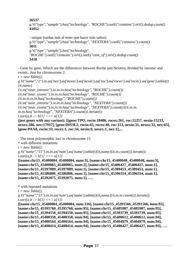
36537g.V("type","sample").has("technology", "ROCHE").outE("contains").inV().dedup.count()41052
- unique (tardan más al tener que hacer más saltos)g.V("type","sample").has("technology", "NEXTERA").outE("contains").count()3011g.V("type","sample").has("technology", "ROCHE").outE("contains").inV().outE("case_of").inV().dedup.count()3418
- Gene by gene, Which are the differences between Roche and Nextera, divided by intronic and exonic. Just for chromosome 2.t = new Table(); g.V("name","2").in.as('nex').as('nexex').as('nexin').as('roc').as('rocex').as('rocin').as('gene').table(t){it.name}{it.in("near_intronic").in.in.in.has("technology", "ROCHE").count()}{it.in("near_exonic").in.in.in.has("technology", "ROCHE").count()}{it.in.in.in.in.has("technology", "ROCHE").count()}{it.in("near_intronic").in.in.in.has("technology", "NEXTERA").count()}{it.in("near_exonic").in.in.in.has("technology", "NEXTERA").count()}{it.in.in.in.in.has("technology", "NEXTERA").count()}.iterate(); t.sort{a,b -> b[1] <=> a[1]}(just genes with any variant): [[gene:TPO, rocin:18486, rocex:261, roc:21257, nexin:15233, nexex:286, nex:17937], [gene:DIS3L2, rocin:43, rocex:40, roc:113, nexin:31, nexex:32, nex:65],[gene:PAX8, rocin:33, rocex:1, roc:34, nexin:0, nexex:1, nex:1],...
- The most polymorphic loci in chromosome 15* with different mutationst = new Table(); g.V("name","15").in.in.as('num').as('name').table(t){it.name}{it.in.count()}.iterate(); t.sort{a,b -> b[1] <=> a[1]}[[name:chr15_45400084_45400084, num:3], [name:chr15_45400048_45400048, num:3], [name:chr15_45400065_45400065, num:2], [name:chr15_45406427_45406427, num:1], [name:chr15_45397889_45397889, num:1], [name:chr15_45389453_45389453, num:1], [name:chr15_45386806_45386806, num:1], [name:chr15_45396354_45396354, num:1], [name:chr15_45392075_45392075, num:1], ….
* with repeated mutationst = new Table(); g.V("name","15").in.in.as('num').as('name').table(t){it.name}{it.in.in.count()}.iterate(); t.sort{a,b -> b[1] <=> a[1]}[[name:chr15_45400084_45400084, num:116], [name:chr15_45391566_45391566, num:95], [name:chr15_45395760_45395760, num:95], [name:chr15_45405987_45405987, num:95], [name:chr15_45394550_45394550, num:95], [name:chr15_45393739_45393739, num:95], [name:chr15_45400358_45400358, num:94], [name:chr15_45400612_45400612, num:94], [name:chr15_45400164_45400164, num:94], [name:chr15_45404979_45404979, num:94], [name:chr15_45408414_45408414, num:94], [name:chr15_45406427_45406427, num:93], ….
Page 37
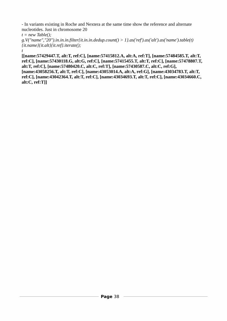
- In variants existing in Roche and Nextera at the same time show the reference and alternate nucleotides. Just in chromosome 20t = new Table(); g.V("name","20").in.in.in.filter{it.in.in.dedup.count() > 1}.as('ref').as('alt').as('name').table(t){it.name}{it.alt}{it.ref}.iterate(); t[[name:57429447.T, alt:T, ref:C], [name:57415812.A, alt:A, ref:T], [name:57484585.T, alt:T, ref:C], [name:57430118.G, alt:G, ref:C], [name:57415455.T, alt:T, ref:C], [name:57478807.T, alt:T, ref:C], [name:57480420.C, alt:C, ref:T], [name:57430587.C, alt:C, ref:G], [name:43058256.T, alt:T, ref:C], [name:43053014.A, alt:A, ref:G], [name:43034783.T, alt:T, ref:C], [name:43042364.T, alt:T, ref:C], [name:43034693.T, alt:T, ref:C], [name:43034660.C, alt:C, ref:T]]
Page 38
5 DiscussionIn the course of the internship some issues have been recurrent because they have generated doubts about the best way to deal with them. These are the most important of them.
5.1 Visualization of resultsNot always it is necessary a graphic visualization of our results. On a daily basis the most usable outcome is a text file enclosing the results. But in complex queries and in a surf mode we think it is necessary an advanced visualization mode.Sometimes the amount of information to represent as “balls and arrows” is huge and impossible to show in a window. But there are ways to condense and show the information in better ways.For us an important issue in the visualization is the mouse interaction with the graph. We think that is very important to click over the vertexes and edges in order to move or obtain information
5.2 Scheme databaseAs we said before, scheme is not a “must be” in a graph oriented database, but we think that a scheme must be created, although it is drawn just in a paper. This is in this way because people needto know how to query the information in the database, need to know which are the types of the nodes and the name of the edges are used to connect them. Of course the users must know the philosophy behind the way the vertexes are connected.
5.3 Mutations graph styleIf we focus our attention in the structure of the graph is easy to notice that it is integrated by three trees:
- tree whose parent vertex is the patient: patient → sample → mutationInSample- tree whose parent vertex is the chromosome: chromosome → gene → locus → mutation → mutationInSample- tree whose father vertex is the HPO: HPO1 →HPO2 → … → HPOn
In addition to this we have the genesets that comprise genes, but they don't form a tree because the same geneset contains several genes and same gene can be in different genesets.
Due to the information is organized in this way there is not relation between same type nodes. When you are traversing a graph it is useful to find paths between nodes of same type: minimum path between two underground stations, all paths of at most 4 jumps between two metabolites whichare related with a chemical reaction. In our contest this is not possible; we cannot obtain this kind ofinformation.This is the reason we think it is a good idea to add to the graph all the information we have about interactions between proteins.
Page 39
5.4 Advantages and limitations of graph database approach
Returning to previous section we have noticed that in the most of the useful queries for the clinical practice what we most use is queries like: “give me the vertexes with the property x like this” or “give me the vertexes belonging to this other vertex”, but not more there.For this kind of queries we don't obtain advantage with the graph database approach. But, of course,these queries can be done and work without problem.In queries with much more data is when we will take advantage of graph oriented database. More inqueries when we use a intense graph traversal (minimum path between vertexes, for example)With time, when the kind of information into the database will be increased (metabolic routes, protein interactions, other kind of samples …) the complexity of the queries will grow [13].In this field it is necessary to do more benchmarking to decide what approach is better for each case.
5.5 MultithreadingWe have noticed a growth in performance when we have installed the database in the cluster scenario, respect when it was in a local scenario. This is because the queries over a graph are suitable for dividing into different threads. We have seen it mainly in experimental queries where path finding was involved.
5.6 Sharding
It will be necessary to evaluate this aspect when the database becomes very big. Then we will see if the indirect sharding given by Hadoop is enough or it would be better to try another one.
Page 40
6 Conclusions
We have dealt with the world of the mutations and the graph databases. We have found big advantages by using this approach.We didn't find too many drawbacks, because we can do all what we can do with the relational databases with the graph databases. Maybe some simple queries, very fast in SQL models, are not as fast as in SQL databases, but it is not very important in INGEMM queries.
A huge advantage when you deal with graph databases is that it is very easy and fast to dive into thegraph. All queries strongly related with vertex relations, with paths between nodes are much faster than with other approach.
In the specific case of Titan database there is an advantage with flexibility in modify the database information. It is easy to add, erase, update and reconnect nodes. There are not restrictions with what you do with a vertex. The only subject a little bit tricky is the way it manages the edges. We have to take care in not to repeat them because it is not easy to query to the system about it.
Now we can afford problems that was complicated and very time consuming. We can compile all the information coming from the NGS pipeline and the query in a way we wasn't be able to do before.The database will be able to grow because we are using HADOOP that is a peace of software whichpermits a high scalability.
6.1 Future uses and improvements
In the bioinformatic section of INGEMM we are obtaining information just from genomic data: NGS analysis (variants). Checking other approaches, like “Knowledge boosting: a graph-based integration approach with multi-omics data and genomic knowledge for cancer clinical outcome prediction” [17], we think we can obtain a big improvement in the diagnostic. It is possible to add information about methylation, miRNA, gene expression, metabolic analysis. Of course this is expensive, but if in any moment we have test like these ones, it will be very easy to add to our database and relate with the contained data.
In case we would want to use the application like a decision system: “We introduce the samples of aperson and the system tells us what kind of disease the patient can develop” we would need to add extra information about the environment in which the patient is involved. This is very important because many diseases are multifactorial diseases, I mean, not only genetic factors are involved, butenvironmental factors too. It is important to know how the patient lives: what the patient eats?, which is the chemical exposure?, is a sporty person?, is a stressed person?, which is the exposure to the solar rays?, …All these factors should take part in the graph. It'd be connected with the patient's node. And could be query like the other information in the graph.
If, as we have mentioned before, existing database data will want to be added: protein interaction, metabolic pathways... There are a lot of databases based in RDF [36], that can be queried with SPARQL [35]: UniProt: (http://beta.sparql.uniprot.org/), Bio2RDF (http://bio2rdf.org/) that
Page 41
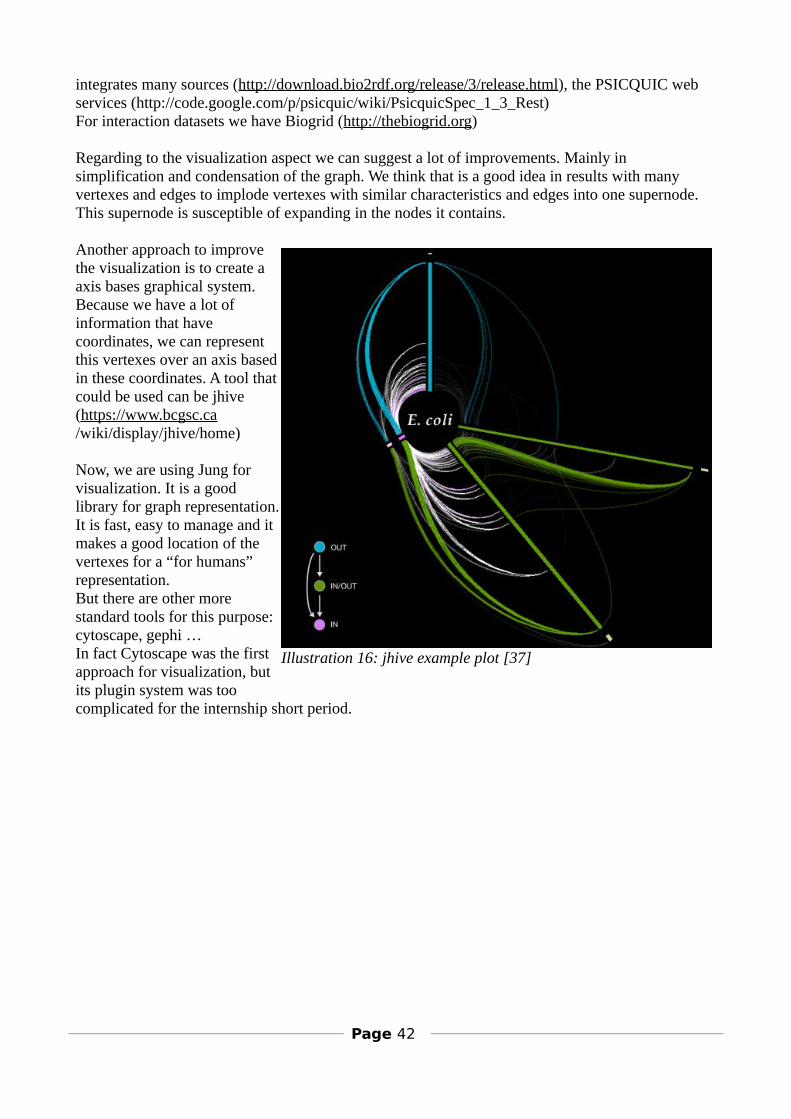
integrates many sources (http://download.bio2rdf.org/release/3/release.html), the PSICQUIC web services (http://code.google.com/p/psicquic/wiki/PsicquicSpec_1_3_Rest) For interaction datasets we have Biogrid (http://thebiogrid.org)
Regarding to the visualization aspect we can suggest a lot of improvements. Mainly in simplification and condensation of the graph. We think that is a good idea in results with many vertexes and edges to implode vertexes with similar characteristics and edges into one supernode. This supernode is susceptible of expanding in the nodes it contains.
Another approach to improvethe visualization is to create aaxis bases graphical system.Because we have a lot ofinformation that havecoordinates, we can representthis vertexes over an axis basedin these coordinates. A tool thatcould be used can be jhive(https://www.bcgsc.ca/wiki/display/jhive/home)
Now, we are using Jung forvisualization. It is a goodlibrary for graph representation.It is fast, easy to manage and itmakes a good location of thevertexes for a “for humans”representation.But there are other morestandard tools for this purpose:cytoscape, gephi …In fact Cytoscape was the firstapproach for visualization, butits plugin system was toocomplicated for the internship short period.
Page 42
Illustration 16: jhive example plot [37]
7 Bibliography[1] Ángela del Pozo, Juan Carlos Silla, Kristina Ibáñez. Internal presentation of the bioinformatic section for INGEMM (2013)
[2] Andrzej Kochański. Pathogenic mutations and non-pathogenic DNA polymorphisms in the mostcommon neurodegenerative disorders (2007)
[3] MiSeq System. Focused power. Speed and simplicity for targeted and small genome sequencing.Illumina (2014)
[4] FASTQ Format Specification (http://maq.sourceforge.net/fastq.shtml)
[5] FASTQC application (http://www.bioinformatics.babraham.ac.uk/projects/fastqc/ )
[6] Bowtie application (http://bowtie-bio.sourceforge.net/index.shtml )
[7] Sequence Alignment/Map Format SpecificationThe SAM/BAM Format Specification Working Group (2014)(https://www.google.es/url?sa=t&rct=j&q=&esrc=s&source=web&cd=1&ved=0CCIQFjAA&url=http%3A%2F%2Fsamtools.github.io%2Fhts-specs%2FSAMv1.pdf&ei=wEnzU6G0LITF0QXcyoH4Aw&usg=AFQjCNHXjACKtEE_s3pBXGWX4sj_E4puJg&sig2=D8y-6Rcg3jOekaV6Wg8PqA&bvm=bv.73231344,d.d2k&cad=rja )
[8] GATK application (https://www.broadinstitute.org/gatk/ )
[9] Tom Strachan, Andrew Read. Human molecular genetics. Fourth edition (2010).
[10] vcf file format (http://www.1000genomes.org/wiki/Analysis/Variant%20Call%20Format/vcf-variant-call-format-version-41)
[11] Deleterious Genes (http://evolution.berkeley.edu/evosite/evo101/IIIE6bBadgenes.shtml)
[12] The Genetic Code (http://biology.kenyon.edu/courses/biol114/Chap05/Chapter05.html)
[13] The Graph Traversal Pattern (http://arxiv.org/abs/1004.1001)
[14] Document from the INGEMM to the bioinformatic master describing the objective of the internship. proyecto_BD_grafos_INGEMM_2014.doc
[15] DbSNP (www.ncbi.nlm.nih.gov/projects/SNP)
[16] Ian Robinson, Jim Webber, Emil Eifrem. GraphDatabases Early Release. Editorial O'Reilly (2013)
[17] Dokyoon Kim, Je-Gun Joung, Kyung-Ah Sohn, Hyunjung Shin, Yu Rang Park,Marylyn D Ritchie, Ju Han Kim. Knowledge boosting: a graph-based integration approach with multi-omics data and genomic knowledge for cancer clinical outcome prediction (2014)
[18] David L. Gibbs, Lisa Gralinski, [...], and Shannon K. McWeeney. Multi-omic network
Page 43
signatures of disease (2013)
[19] STITCH 4.0: Chemical-Protein Interactions (http://stitch.embl.de/)
[20]. MGV: a generic graph viewer for comparative omics data. (http://www.ncbi.nlm.nih.gov/pubmed/21666268)
[21] Cytoscape (http://www.cytoscape.org/what_is_cytoscape.html)
[22] Kathryn Doroschak. DREU Participant Tufts University B.S. Computer Science StudentUniversity of Minnesota (2013) (https://parasol.tamu.edu/dreu2013/Doroschak/)
[23] What is a gene mutation and how do mutations occur? (http://ghr.nlm.nih.gov/handbook/mutationsanddisorders/genemutation)
[24] IRB Primer: Incidental and Secondary Findings (2013)(https://www.google.es/url?sa=t&rct=j&q=&esrc=s&source=web&cd=1&ved=0CCgQFjAA&url=http%3A%2F%2Fbioethics.gov%2Fsites%2Fdefault%2Ffiles%2FIRB%2520Primer%2520-%2520Incidental%2520and%2520Secondary%2520Findings.pdf&ei=-rUEVIi_LM3kaLGrgogH&usg=AFQjCNF7W1Xi-ZP-qkHP1stGY70mufm0dg&sig2=T5907yO4pJ_DdaRLzqeajQ&bvm=bv.74115972,d.d2s&cad=rja)
[25] Burrows-Wheeler Aligner (http://bio-bwa.sourceforge.net/)
[26] Titan graph (http://thinkaurelius.github.io/titan/)
[27] Gremlin language (https://github.com/tinkerpop/gremlin/wiki)
[28] Elasticsearch ( http://www.elasticsearch.org/)
[29] HBASE (http://hbase.apache.org/)
[30] Hadoop (http://hadoop.apache.org/)
[31] Jung framework (http://jung.sourceforge.net/)
[32] Christian Theil Have and Lars Juhl Jensen. Are graph databases ready for bioinformatics? (2013)
[33] graph databases summary http://www.predictiveanalyticstoday.com/top-graph-databases/ (http://en.wikipedia.org/wiki/Graph_database)
[34] Neo4j (http://www.neo4j.org)
[35] SPARQL query language for RDF (http://www.w3.org/TR/rdf-sparql-query/)
[36] Resource Description Framework (RDF) (http://www.w3.org/RDF/)
Page 44
[37] jhive graph representation image (http://www.hiveplot.net/img/web-title-large.png)
[38] Alberts, Bruce, et al. Molecular Biology of the Cell, 5th ed. New York: Garland Publishing, 2000.
[39] An introduction to Next-generation Sequencing Technology. Illumina.( http://res.illumina.com/documents/products/illumina_sequencing_introduction.pdf )
[40] Mark Graves, Ellen R. Bergeman, Charles B. Lawrence. Department of Cell Biology, Baylor College of Medicine. Graph Database Systems for Genomics.
[41] Nygel Small. Py2neo API (http://nigelsmall.com/py2neo/1.6/ )
[42] ArangoDB database (https://www.arangodb.org/ )
[43] Starsity Technologies. High-performance human solutions for Extreme Data( http://sparsity-technologies.com/ )
[44] Stinger libraries (http://www.stingergraph.com/)
[45] Boost libraries (http://www.boost.org/ )
[46] Blueprints (https://github.com/thinkaurelius/titan/wiki/Blueprints-Interface )
[47] Jung libraries. FRLayout (http://jung.sourceforge.net/doc/api/edu/uci/ics/jung/algorithms/layout/FRLayout.html)
[48] Atherly, Alan G., Jack R. Girton, and John F. McDonald. The Science of Genetics. Philadelphia, PA: Saunders College Publishing, 1998.
[49] Cooper, D. N. Human Gene Mutation. Bios Scientific Publishers Ltd., 1997.
[50] Griffiths Anthony J. F. , William M. Gelbart, Jeffrey H. Miller and Richard Lewontin (1999).Mutational Analysis. In Modern Genetic Analysis. W. H. Freeman and Company ISBN 0-7167-3597-0.
[51] Griffiths Anthony J. F. , William M. Gelbart, Jeffrey H. Miller and Richard Lewontin (1999).The Molecular Basis of Mutation. In Modern Genetic Analysis. W. H. Freeman and Company ISBN 0-7167-3597-0.
Page 45
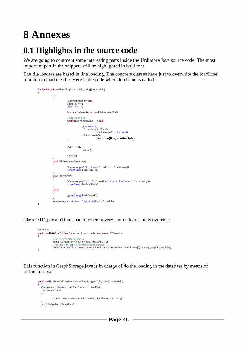
8 Annexes
8.1 Highlights in the source codeWe are going to comment some interesting parts inside the Urdimbre Java source code. The most important part in the snippets will be highlighted in bold font.
The file loaders are based in line loading. The concrete classes have just to overwrite the loadLine function to load the file. Here is the code where loadLine is called:
final public void loadFromFile(String strFile, String[] anotherInfo){
try{
BufferedReader br = null;String line = "";_lineCount = 0;
br = new BufferedReader(new FileReader(strFile));
// One line is readwhile ((line = br.readLine()) != null){
_lineCount ++;if ((_lineCount%100)==0)
Window.output(""+_lineCount);if (!line.isEmpty())
loadLine(line, anotherInfo);}
if (br != null)br.close();
finishing();}catch (FileNotFoundException e){
Window.output("File not found " + strFile + ": " + e.toString());_graphStorage.batchRollBack();
}catch (Exception e){
Window.output("Fail on file " + strFile + " line " + _lineCount + ": " + e.toString());_graphStorage.batchRollBack();
}finally{
_graphStorage.batchCommit();}Window.output(_lineCount + " lines loaded in file:" + strFile);
}
Class OTF_patsamTitanLoader, where a very simple loadLine is override:
@Override
public void loadLine(final String line, String[] anotherInfo) throws IOException{
//The line is splitted in commasString[] splittedLine = fillEmptyFields(line.split(","), 2);//The edge with the previous vertex created is added(new Connection( "from", new Sample( splittedLine[1]), new Patient( splittedLine[0]))).commit( _graphStorage, false);
}
This function in GraphStorage.java is in charge of do the loading in the database by means of scripts in Java:
public void loadFileWithJavaFile(String strFile, String javaFile, String[] anotherInfo){ Window.output("Reading..."+strFile+" with .... " + javaFile); String content = null; try {
content = new Scanner(new File(javaFile)).useDelimiter("\\Z").next(); } catch (FileNotFoundException e1)
Page 46
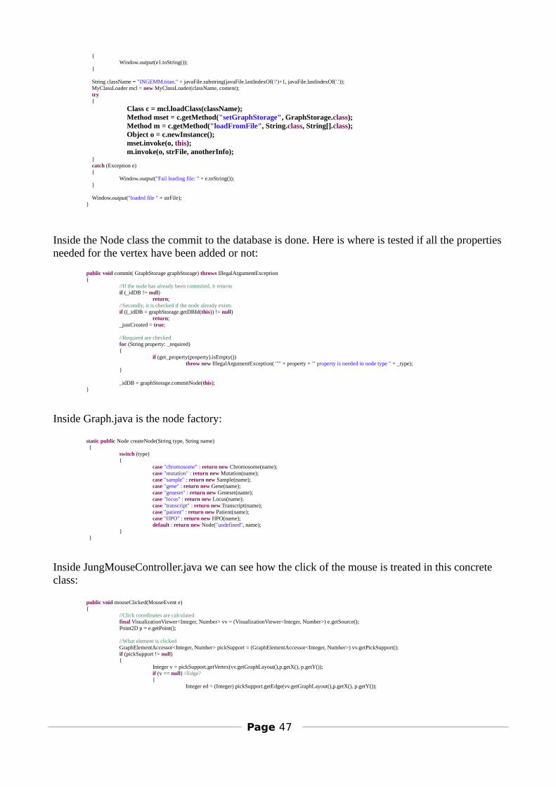
{ Window.output(e1.toString()); }
String className = "INGEMM.titan." + javaFile.substring(javaFile.lastIndexOf('/')+1, javaFile.lastIndexOf('.')); MyClassLoader mcl = new MyClassLoader(className, content); try {
Class c = mcl.loadClass(className); Method mset = c.getMethod("setGraphStorage", GraphStorage.class); Method m = c.getMethod("loadFromFile", String.class, String[].class);
Object o = c.newInstance(); mset.invoke(o, this); m.invoke(o, strFile, anotherInfo);
} catch (Exception e) { Window.output("Fail loading file: " + e.toString()); }
Window.output("loaded file " + strFile);}
Inside the Node class the commit to the database is done. Here is where is tested if all the propertiesneeded for the vertex have been added or not:
public void commit( GraphStorage graphStorage) throws IllegalArgumentException{
//If the node has already been commited, it returnsif (_idDB != null)
return;//Secondly, it is checked if the node already existsif ((_idDB = graphStorage.getDBId(this)) != null)
return;_justCreated = true;
//Required are checkedfor (String property: _required){
if (get_property(property).isEmpty())throw new IllegalArgumentException( "'" + property + "' property is needed in node type " + _type);
}
_idDB = graphStorage.commitNode(this);}
Inside Graph.java is the node factory:
static public Node createNode(String type, String name) {
switch (type){
case "chromosome" : return new Chromosome(name);case "mutation" : return new Mutation(name);case "sample" : return new Sample(name);case "gene" : return new Gene(name);case "geneset" : return new Geneset(name);case "locus" : return new Locus(name);case "transcript" : return new Transcript(name);case "patient" : return new Patient(name);case "HPO" : return new HPO(name);default : return new Node("undefined", name);
} }
Inside JungMouseController.java we can see how the click of the mouse is treated in this concrete class:
public void mouseClicked(MouseEvent e) {
//Click coordinates are calculatedfinal VisualizationViewer<Integer, Number> vv = (VisualizationViewer<Integer, Number>) e.getSource();Point2D p = e.getPoint();
//What element is clickedGraphElementAccessor<Integer, Number> pickSupport = (GraphElementAccessor<Integer, Number>) vv.getPickSupport();if (pickSupport != null) {
Integer v = pickSupport.getVertex(vv.getGraphLayout(),p.getX(), p.getY());if (v == null) //Edge?{
Integer ed = (Integer) pickSupport.getEdge(vv.getGraphLayout(),p.getX(), p.getY());
Page 47
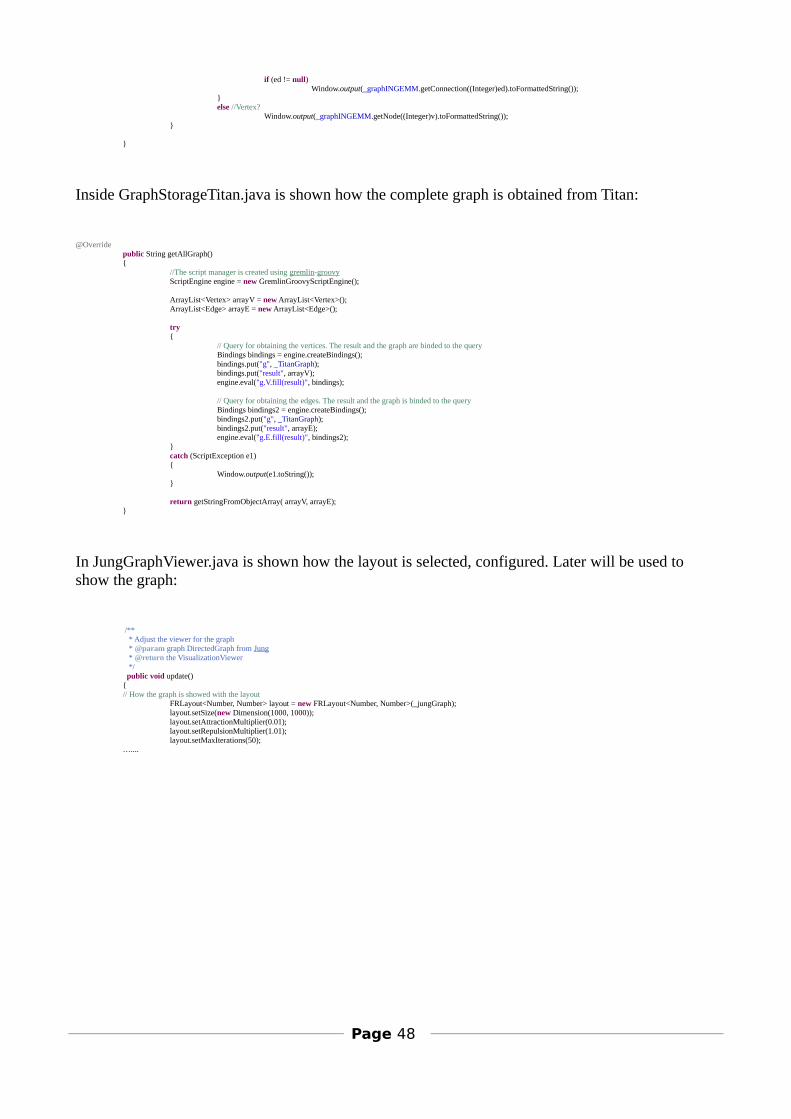
if (ed != null)Window.output(_graphINGEMM.getConnection((Integer)ed).toFormattedString());
}else //Vertex?
Window.output(_graphINGEMM.getNode((Integer)v).toFormattedString());}
}
Inside GraphStorageTitan.java is shown how the complete graph is obtained from Titan:
@Overridepublic String getAllGraph(){ //The script manager is created using gremlin-groovy
ScriptEngine engine = new GremlinGroovyScriptEngine();
ArrayList<Vertex> arrayV = new ArrayList<Vertex>();ArrayList<Edge> arrayE = new ArrayList<Edge>();
try{
// Query for obtaining the vertices. The result and the graph are binded to the queryBindings bindings = engine.createBindings();bindings.put("g", _TitanGraph);bindings.put("result", arrayV);engine.eval("g.V.fill(result)", bindings);
// Query for obtaining the edges. The result and the graph is binded to the queryBindings bindings2 = engine.createBindings();bindings2.put("g", _TitanGraph);bindings2.put("result", arrayE);engine.eval("g.E.fill(result)", bindings2);
}catch (ScriptException e1){ Window.output(e1.toString());}
return getStringFromObjectArray( arrayV, arrayE);}
In JungGraphViewer.java is shown how the layout is selected, configured. Later will be used to show the graph:
/** * Adjust the viewer for the graph * @param graph DirectedGraph from Jung * @return the VisualizationViewer */ public void update(){
// How the graph is showed with the layoutFRLayout<Number, Number> layout = new FRLayout<Number, Number>(_jungGraph);layout.setSize(new Dimension(1000, 1000));layout.setAttractionMultiplier(0.01);layout.setRepulsionMultiplier(1.01);layout.setMaxIterations(50);
…....
Page 48