6.1

Derivatives Analysis & Valuation (Futures) Study Session 6

LOS 1 : Introduction

Define Forward Contract, Future Contract.

Forward Contract, In Forward Contract one party agrees to buy, and the counterparty to sell, a physical asset or a security at a specific price on a specific date in the future. If the future price of the assets increases, the buyer(at the older, lower price) has a gain, and the seller a loss.

Futures Contract is a standardized and exchange-traded. The main difference with forwards are that futures are traded in an active secondary market, are regulated, backed by the clearing house and require a daily settlement of gains and losses.

Future Contracts differ from Forward Contracts in the following ways:

Future Contracts Forward Contracts Organized Exchange Private Contracts Highly Standardized Lot size requirement Expiry Date MTM

Customized Contracts

No Counterparty default risk Counterparty default risk exists Government Regulated Usually not Regulated

6.2

LOS 2 : Position to be taken under Future Market

How to settle / square-off / covering / closing out a position to calculate Profit/ Loss

Long Position Short position

Short Position Long position

LOS 3 : Gain or Loss under Future Market

Position If Price on Maturity/ Settlement Price Gain/ Loss

Long Position Increase Gain Decrease Loss

Short Position Increase Loss Decrease Gain

Note: Gain/Loss is net of brokerage charge. Brokerage is paid on both buying & selling. Security Deposit is not considered while calculating Profit & Loss A/c. Interest paid on borrowed amount must be deducted while calculating Profit & Loss. A Future contract is ZERO-SUM Game. Profit of one party is the loss of other party.

To Square Off

To Square Off

6.3

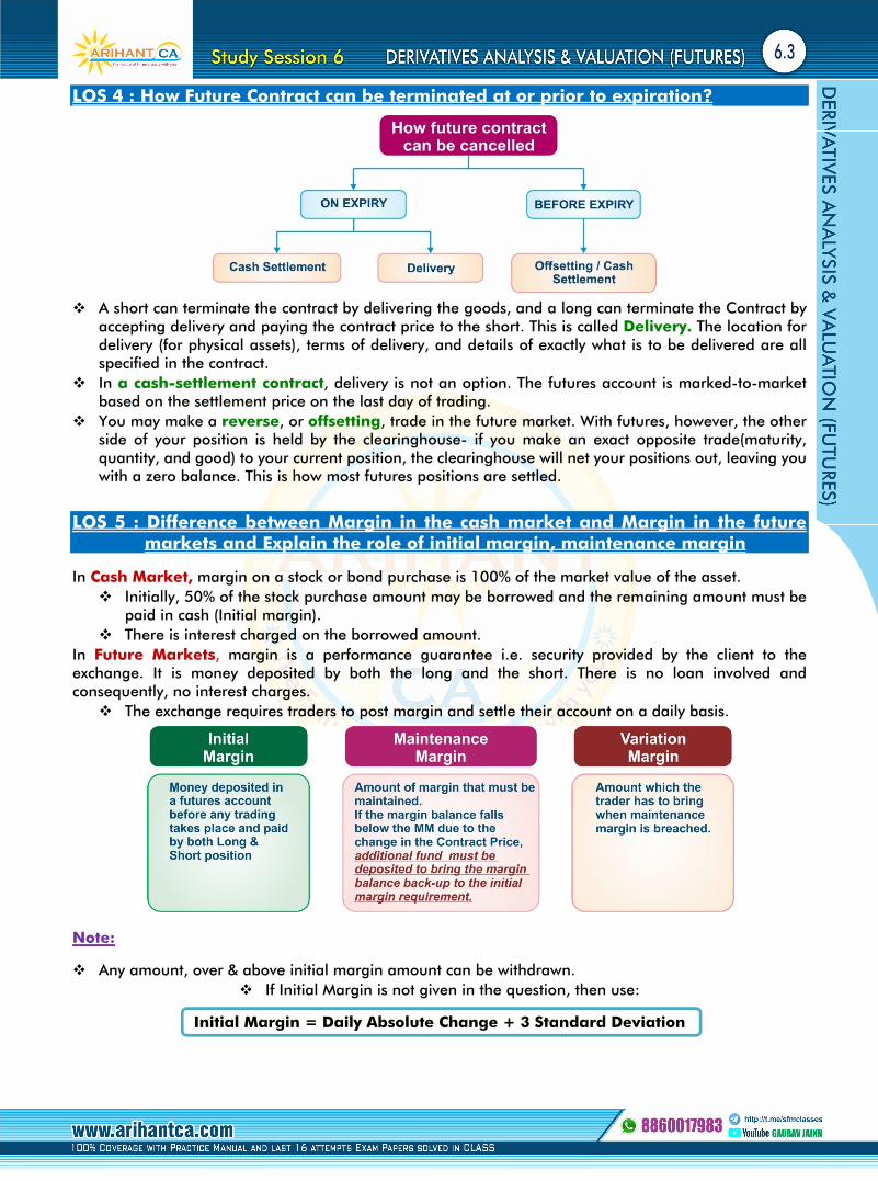
LOS 4 : How Future Contract can be terminated at or prior to expiration?

A short can terminate the contract by delivering the goods, and a long can terminate the Contract by

accepting delivery and paying the contract price to the short. This is called Delivery. The location for delivery (for physical assets), terms of delivery, and details of exactly what is to be delivered are all specified in the contract.

In a cash-settlement contract, delivery is not an option. The futures account is marked-to-market based on the settlement price on the last day of trading.

You may make a reverse, or offsetting, trade in the future market. With futures, however, the other side of your position is held by the clearinghouse- if you make an exact opposite trade(maturity, quantity, and good) to your current position, the clearinghouse will net your positions out, leaving you with a zero balance. This is how most futures positions are settled.

LOS 5 : Difference between Margin in the cash market and Margin in the future markets and Explain the role of initial margin, maintenance margin

In Cash Market, margin on a stock or bond purchase is 100% of the market value of the asset. Initially, 50% of the stock purchase amount may be borrowed and the remaining amount must be

paid in cash (Initial margin). There is interest charged on the borrowed amount.

In Future Markets, margin is a performance guarantee i.e. security provided by the client to the exchange. It is money deposited by both the long and the short. There is no loan involved and consequently, no interest charges. The exchange requires traders to post margin and settle their account on a daily basis.

Note:

Any amount, over & above initial margin amount can be withdrawn. If Initial Margin is not given in the question, then use:

Initial Margin = Daily Absolute Change + 3 Standard Deviation

6.4

LOS 6 : Concept of Compounding

Example: Computing EAR for Range of compounding frequency.

Using a stated rate of 6%, compute EARs for semi-annual, quarterly, monthly and daily compounding.

Solution:

EAR with :

Semi-annual Compounding = (1+0.03) 2 – 1 = 1.06090 – 1 = 0.06090 = 6.090% Quarterly compounding = (1+0.015) 4 – 1 = 1.06136 – 1 = 0.06136 = 6.136% Monthly Compounding = (1+0.005) 12 – 1 = 1.06168 – 1 = 0.06168 = 6.168% Daily Compounding = (1+0.00016438) 365 – 1 = 1.06183 – 1 = 0.06183 = 6.183%

Notice here that the EAR increases as the compounding frequency increases.

Concept of e rt & e –rt (Continuous Compounding)

Most of the financial variable such as Stock price, Interest rate, Exchange rate, Commodity price change on a real time basis. Hence, the concept of Continuous compounding comes in picture.

Continuous Compounding means compounding every moment. Instead of (1 + r) we will use ert

How to Calculate e rt & e –rt

Example:

e0 = 1 e.25 = 1.28403 e-.25 = 0.77880 or . = 0.77880

e .205 = ? e .20 = 1.22140 e.21 = 1.23368 . .

1.22754

Calculation of ab

1. √𝒂 12 Times 2. - 1 3. × b 4. + 1 5. × = 12 Times

Calculation of eb

1. √𝒆 12 Times 2. - 1 3. × b 4. + 1 5. × = 12 Times Hint : e1 = 2.71828

6.5

e .357 = ? e .35 = 1.41907 e .36 = 1.43333 Since 3rd digit is not 5, in this case we have to use interpolation technique:when power of e increases by 0.01, then value increase by 0.01426 [1.43333 – 1.41907]

when power of e increases by 1, then value increases by . .

when power of e increases by 0.007, then value increases by . . ×

0.007 = 0.00998 Value of e .357 = 1.41907 + 0.00998 = 1.42905

e - .357 = . = 0.69977

LOS 7 : Fair future price of security with no income

In case of Normal Compounding

Fair future price = Spot Price (1+r)n

In case of Continuous Compounding

Fair future price = Spot Price × e rt

Where r = risk free interest p.a. with Continuous Compounding. t = time to maturity in years/ days. (No. of days / 365) or (No. of months / 12)

LOS 8 : Fair Future Price of Security with Dividend Income

6.6

In case of Normal Compounding

Fair Future Price = [Spot Price – PV of Expected Dividend ] ( 1+r)n

In case of Continuous Compounding

Fair Future Price = [Spot Price – PV of Expected Dividend ] × e r t

PV of DI = Present Value of Dividend Income = Dividend × e – r t Where t = period of dividend payments

LOS 9 : Fair Future Price of security when income is expressed in percentage or when dividend yield is given

In case of Normal Compounding

Fair Future Price = Spot Price [1+(r-y)] n

In case of Continuous Compounding

Fair Future Price = Spot Price × e(r-y) × t

Where y = income expressed in % or dividend Yield

LOS 10 : Fair Future Price of Commodity with storage cost

In case of Normal Compounding

Fair Future Price = [Spot Price + PV of S.C ] ( 1+r) n

In case of Continuous Compounding

Fair Future Price = [Spot Price + PV of S.C ] × e rt

Where PV of S.C = Present Value of Storage Cost

Note: Fair Future Price when Storage Cost is given in percentage(%).

FFP = Spot Price × e (r + s) × t

Where S = Storage cost expressed in percentage.

LOS 11 : Fair Future Price of commodities with Convenience yield expressed in % (Similar to Dividend Yield)

The benefit or premium associated with holding an underlying product or physical good rather than contract or derivative product i.e. extra benefit that an investor receives for holding a commodity.

6.7

In case of Continuous Compounding

Fair Future Price = Spot Price × e(r-c)×t

Note: Fair Future Price when convenience income is expressed in Absolute Amount.

Fair Future Price = [Spot Price - PV of Convenience Income] × e rt

LOS 12 : Arbitrage Opportunity between Cash and Future Market

Arbitrage is an important concept in valuing (Pricing) derivative securities. In its Purest sense, arbitrage is riskless.

Arbitrage opportunities arise when assets are mispriced. Trading by Arbitrageurs will continue until they effect supply and demand enough to bring asset prices to efficient( no arbitrage) levels.

Arbitrage is based on “Law of one price”. Two securities or portfolios that have identical cash flows in future, should have the same price. If A and B have the identical future pay offs and A is priced lower than B, buy A and sell B. You have an immediate profit.

Difference between Actual Future Price and Fair Future Price?

Fair Future Price is calculated by using the concept of Present Value & Future Value. Actual Future Price is actually prevailing in the market. Case Value Future Market Cash Market Borrow/ Invest FFP < AFP Over-Valued Sell or Short Position Buy Borrow FFP > AFP Under-Valued Buy or Long Position Sell # Investment

# Here we assume that Arbitrager already hold shares

LOS 13: Complete Hedging by using Index Futures & Beta

Hedging is the process of taking an opposite position in order to reduce loss caused by Price fluctuation. The objective of Hedging is to reduce Loss. Complete Hedging means profit/ Loss will be Zero.

Position to be taken:

a) Long Position should be hedged by Short Position. b) Short Position should be hedged by Long Position.

Value of Position to be taken:

Value of Position for Complete hedge should be taken on the basis of Beta through index futures.

Value of Position for Complete Hedge = Current Value of Portfolio × Existing Stock Beta

LOS 14: Value of Position for Increasing & Reducing Beta to a Target Level

6.8

Alternative 1 (Hedging Using Index Future)

Step 1 : Decide Position

Case 1 : To Reduce Risk

Long Position Short Index Future

Short Position Long Index Future

Case 2 : To Increase Risk

Long Position Long Index Future

Short Position Short Index Future

Step 2 : Value of Position

Case I: When Existing Beta > Target Beta

Objective: Reducing Risk

Value of Index Position = Value of Existing Portfolio × [Existing Beta – Desired Beta]

Action: Take Short Position in Index & keep your current position unchanged.

Case II: When Existing Beta < Target Beta

Objective: Increase Risk

Value of Index Position = Value of Existing Portfolio × [Desired Beta – Existing Beta]

Action: Take Long Position in Index & keep your current position unchanged

Step 3 : No. of future contracts to be sold or purchased for increasing or reducing Beta to a Desired Level using Index Futures.

No. of Future Contract to be taken = 𝐕𝐚𝐥𝐮𝐞 𝐨𝐟 𝐈𝐧𝐝𝐞𝐱 𝐏𝐨𝐬𝐢𝐭𝐢𝐨𝐧𝐕𝐚𝐥𝐮𝐞 𝐨𝐟 𝐨𝐧𝐞 𝐅𝐮𝐭𝐮𝐫𝐞 𝐂𝐨𝐧𝐭𝐫𝐚𝐜𝐭

Alternative 2 (Hedging Using Risk free Investment or Borrowing)

Case 1: Reducing Risk

SELL SOME SECURITIES AND REPLACE WITH RISK-FREE INVESTMENT

Step1: Equate the weighted Average Beta formulae to the new desired Beta

Target Beta = Beta1 × W1 + Beta2 × W2 ( Beta of Risk free investment is Zero)

Step2: Use the weights and decide

Case 2: Increasing Risk

BUY SOME SECURITIES AND BORROW AT RISK-FREE RATE

Step1: Equate the weighted Average Beta formulae to the new desired Beta

Target Beta = Beta1 × W1 + Beta2 × W2 ( Beta of Risk free investment is Zero)

Step2: Use the weights and decide

6.9

LOS 15 : Partial Hedge

Value of position in Index Future = Value of existing Portfolio × Existing beta × percentage (%) to be Hedge

It result into Over-Hedged or Under-Hedged Position There may be profit or loss depending upon the situation.

LOS 16 : Beta of a Cash and Cash Equivalent

Beta of a cash and Risk free security is Zero.

LOS 17 : Hedging Commodity Risk Through Futures

LOS 18 : Calculation of Rate of Return

Increase or Decrease in Stock Price (P1 – P0) (+) Dividend Received (-) Transaction Cost (-) Interest Paid on Borrowed Amount Net Amount Received

Rate of return = 𝐍𝐞𝐭 𝐀𝐦𝐨𝐮𝐧𝐭 𝐑𝐞𝐜𝐞𝐢𝐯𝐞𝐝𝐓𝐨𝐭𝐚𝐥 𝐈𝐧𝐢𝐭𝐢𝐚𝐥 𝐄𝐪𝐮𝐢𝐭𝐲 𝐈𝐧𝐯𝐞𝐬𝐭𝐦𝐞𝐧𝐭 × 𝟏𝟎𝟎

LOS 19 : Hedge Ratio

The Optional Hedge Ratio to minimize the variance of Hedger’s position is given by:-

Hedge Ratio = Corr. (r) 𝛔𝐒𝛔𝐅

σS = S.D of Δ S σF = S.D of Δ F r = Correlation between Δ S and Δ F Δ S = Change in Spot Price Δ F = Change in Future Price