Derivation of seawater intrusion models

by formal asymptotics

M. Jazar∗, R. Monneaua

March 4, 2014

Abstract

In this paper, we consider the flow of fresh and saltwater in a saturated porous medium in order to describe the

seawater intrusion. Starting from a formulation with constant densities respectively of fresh and saltwater, whose

velocities are proportional to the gradient of pressure (Darcy’s law), we consider the formal asymptotic limit as the

aspect ratio between the thickness and the horizontal length of the porous medium tends to zero. In the limit of

the regime defined by the Dupuit-Forchheimer condition, we identify reduced models of Boussinesq type both in the

cases of unconfined and confined aquifers.

MSC: 35R35, 35B40

Keywords: seawater intrusion, formal asymptotics, porous medium, groundwater flow, Dupuit-Forchheimer,saltwater and freshwater interface, Ghyben-Herzberg relation, confined and unconfined aquifer, shallow wa-ter, Boussinesq equation.

1 Introduction

We are interested in the modeling of seawater intrusion in coastal regions. On the one hand coastal aquiferscontain freshwater and on the other hand saltwater from the sea can enter the ground and replace the fresh-water. This phenomenon can be especially important in coastal regions where there is intensive extractionof freshwater from wells. We refer to [7] for a general overview on seawater intrusion models.

Our main goal is to derive formally simplified (2D) models describing the evolution of the interfacesfreshwater/saltwater and freshwater/dry soil, from common (3D) models of hydrology based on Darcy’s law.

1.1 Setting of the problem

We consider two simple situations: the case of an unconfined aquifer (see Figure 1) and the case of a confinedaquifer (see Figure 2). In each case, the constant seawater level is h1 and the domains are assumed to beunbounded horizontally. The unboundedness of the domains does not create difficulties, because we restrictour approach to a formal level.

1.1.1 The unconfined aquifer

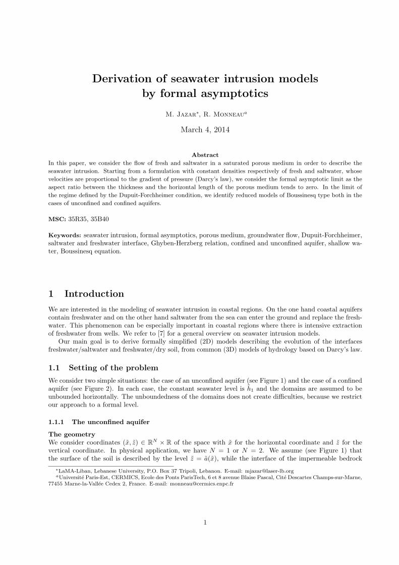
The geometryWe consider coordinates (x, z) ∈ RN × R of the space with x for the horizontal coordinate and z for thevertical coordinate. In physical application, we have N = 1 or N = 2. We assume (see Figure 1) thatthe surface of the soil is described by the level z = a(x), while the interface of the impermeable bedrock

∗LaMA-Liban, Lebanese University, P.O. Box 37 Tripoli, Lebanon. E-mail: mjazar@laser-lb.orgaUniversite Paris-Est, CERMICS, Ecole des Ponts ParisTech, 6 et 8 avenue Blaise Pascal, Cite Descartes Champs-sur-Marne,

77455 Marne-la-Vallee Cedex 2, France. E-mail: monneau@cermics.enpc.fr

1

bedrock

sea

: freshwater

airdry soil

: saltwater

z = a(x)

z = h1

z = b(x)

z = h(t, x)

z = g(t, x)Ωt

f

Ωts

Figure 1: Unconfined aquifer

is described by the level z = b(x), satisfying b < a. We assume that in the porous medium, the interfacebetween the freshwater and the dry soil can be written

Γth=(x, z) ∈ RN × R, z = h(t, x)

,

the interface between the saltwater and the freshwater (which are assumed immiscible) can be written

Γtg =

(x, z) ∈ RN × R, z = g(t, x)

.

In particular these interfaces Γthand Γt

g are unbounded horizontally, and we have the following constraint

(1.1) b ≤ g ≤ h ≤ a on RN .

We assume that all the functions b, g, h, a are smooth enough. We define the open set of freshwater

Ωtf =

(x, z) ∈ RN × R, g(t, x) < z < h(t, x)

and Ωf =

⋃t>0

t× Ωt

f

and the open set of saltwater in the porous medium

Ωts =

(x, z) ∈ RN × R, b(x) < z < g(t, x)

and Ωs =

⋃t>0

t× Ωt

s.

Similarly, we define the open set of the porous medium as

Ωt =(x, z) ∈ RN × R, z < a(x)

and Ω =

⋃t>0

t× Ωt

where in order to keep uniform notations, we use the notation Ωt even if it is independent of t.The PDEsWe set α = f for the freshwater and α = s for the saltwater. We define the density field of the fluid α as

ρα(t, x, z) =

ρ0α if (x, z) ∈ Ωtα

0 otherwise

2

where ρ0α is the mass density of the fluid α (assumed to be a constant with 0 < ρ0f < ρ0s). We also set the

specific weight γα = ρ0αg0 with g0 the standard gravity constant. We assume that ρα solves formally the

following equations

(1.2)

φα(x, z)∂ρα

∂t+ div (ραvα) = 0 on Ωα

vα = −κα(x, z) ∇(p+ γαz) on Ωα

∣∣∣∣∣∣∣ for α = f, s

p is continuous across Γtg

vf · n ≥ 0 on (∂Ωt) ∩ (∂Ωtf )

g ≤ h1 and b < h everywhere

φα∂Fα

∂t+ vα · ∇Fα = 0 on

Fα = 0

∩ Ωα ∩ Ω for Fα + z =

h, g, b if α = f,

g, b if α = s.

Here 0 < φα(x, z) ≤ 1 is the effective porosity of the porous medium, where, in order to simplify for a fullysaturated medium, we assume that the water content is equal to the porosity. Notice that this effectiveporosity φα should be independent of the fluid α, but for sake of generality we allow here such a dependence.

Here p is the pressure assumed to be defined on Ωtf ∪ Ωt

s, and div and ∇ are the divergence and the

gradient, respectively, taken with respect to the coordinates (x, z). Moreover κα(x, z) ∈ R(N+1)×(N+1)sym is a

given symmetric matrix which is positive definite.The quantity vα is the Darcy flux and vα/φα is the velocity vector field of the fluid α. The expression

defining the flux vα follows from Darcy’s law (where κα =kαµα

with µα the dynamic viscosity and kα the

intrinsic permeability tensor of the porous medium). The fourth condition of (1.2) involves the outward

unit normal n to Ωt and means that the flux of freshwater can only go out of the soil (in the absence ofsources), which is very natural. In our proofs, we will need the fifth condition of (1.2), which is a naturalcondition that means in particular that the saltwater in the soil is always below the sea level z = h1. Thesixth condition of (1.2) means that the interface Γt

h is transported by the freshwater velocity vector field, the

interface Γtg is transported by both the fresh and saltwater, and finally both the fresh and saltwater move

tangentially to the bottom z = b.We also assume the following boundary condition

(1.3)

p(t, x, z) =

γs(h1 − z) if z = h(t, x) = a(x) < h1

0 otherwise

h(t, x) = a(x) if a(x) < h1.

The first condition of (1.3) follows from the fact that we assume the atmospheric pressure to be constantand normalized to zero and that the seawater is assumed to be at the hydrostatic equilibrium. We recallthat the surface of the sea is assumed to be at the altitude h1. When the free surface z = h(t, x) has nocontact with the sea, then its pressure is assumed to be equal to the atmospheric pressure zero. The firstand last lines of (1.3) mean that we assume the part a < h1 to be under the seawater level.

1.1.2 The confined aquifer

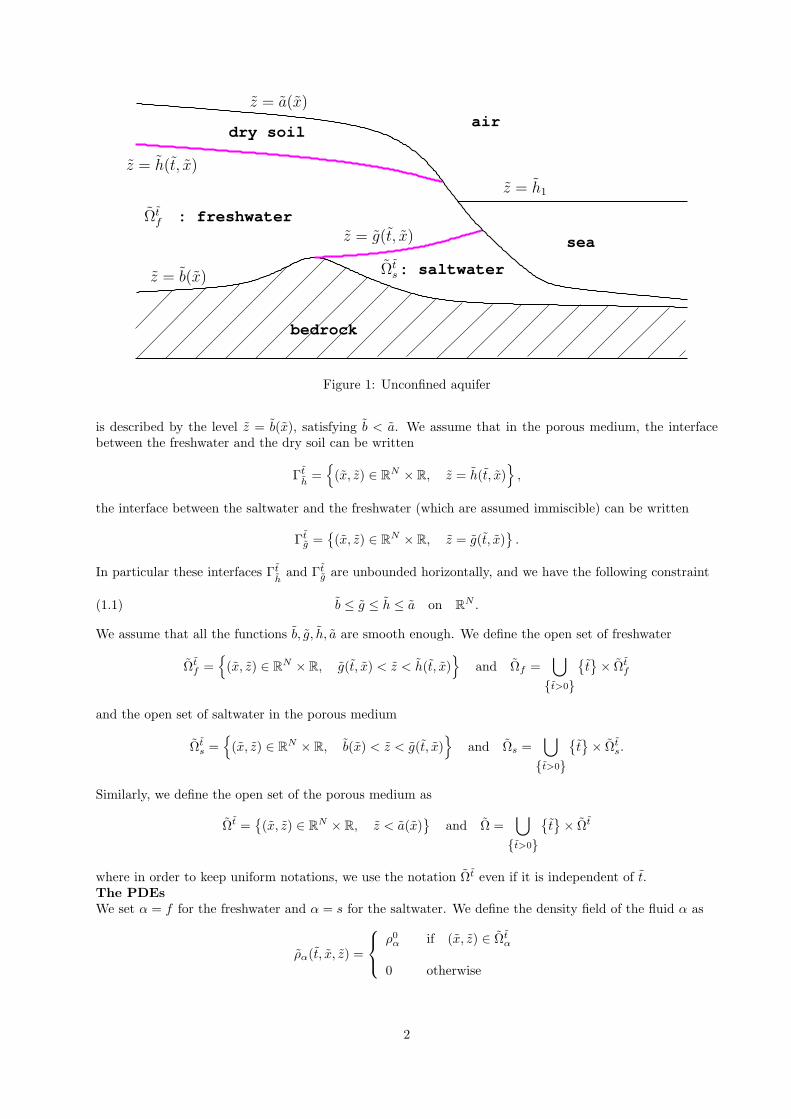
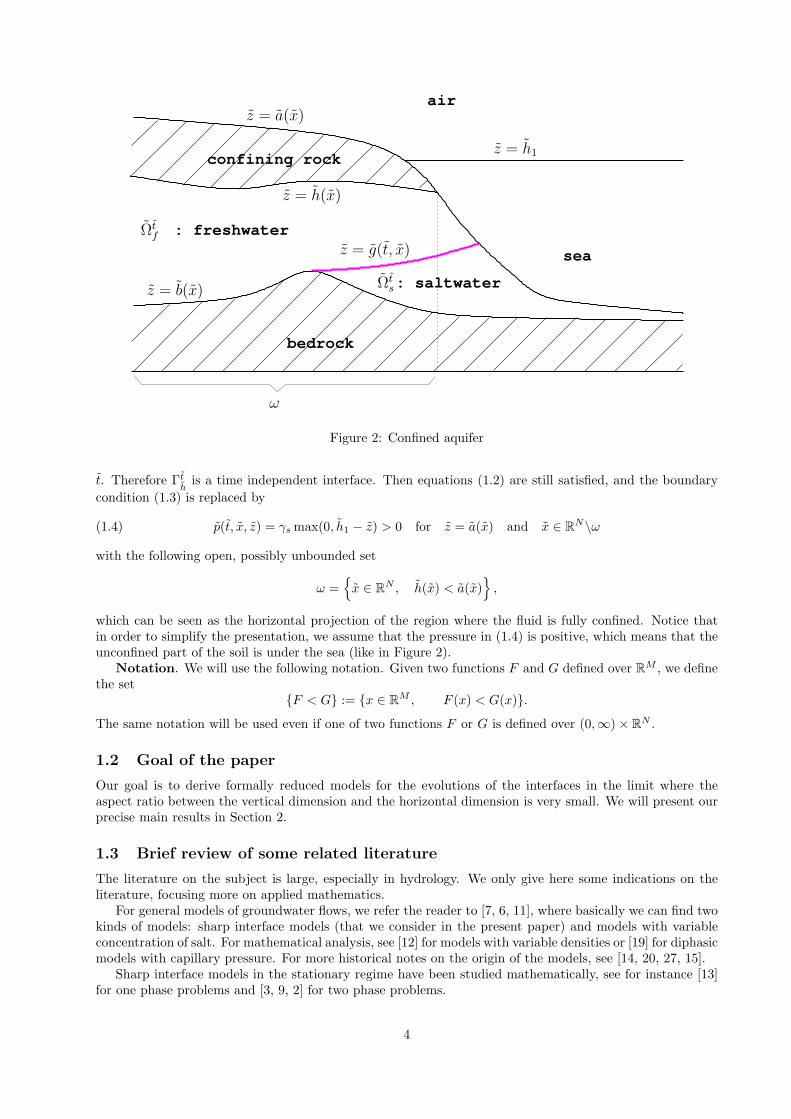
The situation of the confined aquifer is chosen similar to the unconfined aquifer (see Figure 2). In particularwe assume that h1 > h in the neighbourhood of the points x ∈ RN where h = a. This means that thefreshwater only exits the porous medium to go in the seawater. The main difference is that the function h(x)is now a given function describing the shape of the upper confining aquifer and then is independent of time

3

bedrock

sea

: freshwater

: saltwater

air

confining rock

z = a(x)

z = b(x)

z = g(t, x)Ωt

f

Ωts

z = h1

z = h(x)

ω

Figure 2: Confined aquifer

t. Therefore Γthis a time independent interface. Then equations (1.2) are still satisfied, and the boundary

condition (1.3) is replaced by

(1.4) p(t, x, z) = γs max(0, h1 − z) > 0 for z = a(x) and x ∈ RN\ω

with the following open, possibly unbounded set

ω =x ∈ RN , h(x) < a(x)

,

which can be seen as the horizontal projection of the region where the fluid is fully confined. Notice thatin order to simplify the presentation, we assume that the pressure in (1.4) is positive, which means that theunconfined part of the soil is under the sea (like in Figure 2).

Notation. We will use the following notation. Given two functions F and G defined over RM , we definethe set

F < G := x ∈ RM , F (x) < G(x).

The same notation will be used even if one of two functions F or G is defined over (0,∞)× RN .

1.2 Goal of the paper

Our goal is to derive formally reduced models for the evolutions of the interfaces in the limit where theaspect ratio between the vertical dimension and the horizontal dimension is very small. We will present ourprecise main results in Section 2.

1.3 Brief review of some related literature

The literature on the subject is large, especially in hydrology. We only give here some indications on theliterature, focusing more on applied mathematics.

For general models of groundwater flows, we refer the reader to [7, 6, 11], where basically we can find twokinds of models: sharp interface models (that we consider in the present paper) and models with variableconcentration of salt. For mathematical analysis, see [12] for models with variable densities or [19] for diphasicmodels with capillary pressure. For more historical notes on the origin of the models, see [14, 20, 27, 15].

Sharp interface models in the stationary regime have been studied mathematically, see for instance [13]for one phase problems and [3, 9, 2] for two phase problems.

4

For 2D models describing interfaces, we refer the reader to Boussinesq [10] where was derived the porousmedium equation under certain assumptions. See the recent book of Vazquez [35] for a mathematical studyof this equation. Starting from sharp interface models, certain 2D models under certain assumptions arederived in the hydrological literature [5, 8, 18, 4], see also [1, 24] for some applications. Different models arederived in [31, 29, 32] in the framework of variable concentration of salt.

Notice that the method we use to deduce 2D models from 3D models is similar to the one of the derivationof Saint-Venant equations from the Navier-Stokes equations (see [21]).

It is interesting to mention several works about analytical solutions and the comparison between 3Dsolutions and 2D solutions obtained after applying the Dupuit-Forchheimer approximation, see in particular[26, 36, 25, 22, 23]. For more information about analytical solutions, see [28, 30].

We refer to [17] for the analysis of a model similar to (2.6) in the confined case and [33] for the analysis ofa stationary model similar to (2.6),(2.8) (and (2.9)) in the confined case, where existence of weak solutionsis proved.

Finally, for the identification of hydraulic conductivities (as an inverse problem), let us mention forinstance [16].

1.4 Organization of the paper

In Section 2, we present our main results. In Section 3 we prove Theorem 2.2 on the identification of the limitmodels. In Section 4, we prove Theorem 2.3 on the oulet properties, and in Section 5, we prove Theorem2.4 on Ghyben-Herzberg condition. Finally in Section 6 we rewrite the models under special assumptionsand present some explicit particular stationary solutions.

2 Main results

In this section, we will explain how to obtain the reduced model (2.6) presented below, with the matrixgiven by (2.4). To this end, we assume the existence of a small parameter ε > 0 such that the data of theproblem satisfy

(2.1)

x = xz = εzt = t/εa(x) = εa(x)

b(x) = εb(x)

h1 = εh1

φα(x, z) = φα(x, z)

κα(x, z) = κα(x, z) =

κxxα (x, z) κxz

α (x, z)

κzxα (x, z) κzz

α (x, z)

.

The parameter ε can be seen as the aspect ratio between the thickness of the soil (vertical dimension) andthe horizontal length of the soil. When ε is small, the process is very slow and we also have to rescale thetime, in order to observe some evolution of the interfaces.

In order to make precise our result (even if it is only a formal result), we need to consider the followingrescaling:

(2.2)

h(t, x) = εhε(t, x) (with hε(x) given in the confined case)g(t, x) = εgε(t, x)p(t, x, z) = εpε(t, x, z)vxα(t, x) = εvx,εα (t, x)vzα(t, x) = ε2vz,εα (t, x).

Such a scaling may seem arbitrary at a first glance, but it comes out naturally from the formal compu-tations, as the reader can see in the proofs. Moreover, it is very natural to think that the vertical velocityvzα is much smaller than the horizontal velocity vxα, when the aspect ratio ε is very small.Indeed, the two last lines of (2.2) show that the velocity of the fluid is much more horizontal than vertical,

5

which is the Dupuit-Forchheimer assumption (see for instance [34], [24]). We assume the existence of formalasymptotics:

(2.3)

hε = h + εh1 + ε2h2 + ε3h3 + ...gε = g + εg1 + ε2g2 + ε3g3 + ...pε = p + εpε1 + ε2pε2 + ε3pε3 + ...vx,εα = vxα + εvxα,1 + ε2vxα,2 + ε3vxα,3 + ...vz,εα = vzα + εvzα,1 + ε2vzα,2 + ε3vzα,3 + ...

Here we introduced the notation h1, h2, h3, etc. for the functions in the expansion in order to distinguishh1 from the constant h1 defined in (2.1). Notice that this expansion is only formal and we do not intend togive a particular meaning except the one of computer algebra. In this paper, all the computations will becarried out assuming that we are allowed to make them (e.g., if the functions are smooth enough), but neverchecking that they have a special meaning in some particular functional space. Our goal is really to derivenew models, and this is why we decided not to take care of the rigor in the sense of classical mathematicalanalysis.

We define

(2.4) Kα(x, z) = γs

∫ z

0

dz κxxα (x, z) with κxx

α (x, z) = κxxα (x, z)− (κzz

α (x, z))−1κxzα (x, z)κzx

α (x, z).

We also set

Φα(x, z) =

∫ z

0

dz φα(x, z),

and

(2.5) ε0 =γs − γf

γs∈ (0, 1).

This quantity ε0 is usually small (but has nothing to do with the aspect ratio ε).Unconfined aquiferWe have for some open sets Uf , Us of (0,∞)× RN (defined later)

(2.6)

b ≤ g ≤ h ≤ a, b < h and g ≤ h1 on [0,+∞)× RN

(Φf (· , h)− Φf (· , g))t = divx

([Kf (· , z)]z=h

z=g ∇x(p+(1− ε0)h))

on h < a

(Φf (· , h)− Φf (· , g))t ≤ divx

([Kf (· , z)]z=h

z=g ∇x(p+ (1− ε0)h))

on Uf

(Φs(· , g))t = divx ([Ks(· , z)]z=gz=b ∇x(p+(1− ε0)h+ ε0g)) on g < a

(Φs(· , g))t ≤ divx ([Ks(· , z)]z=gz=b ∇x(p+(1− ε0)h+ ε0g)) on Us,

with[Kα(x, z)]

z=z2z=z1

= Kα(x, z2)−Kα(x, z1),

and

(2.7)

h = a on a < h1

p(t, x) = p0(t, x) :=

h1 − a(x) if h = a < h1

0 otherwise.

Confined aquiferWe have (2.6) with

(2.8)

ht = 0

p(t, x) = p0(x) := max(0, h1 − a(x)) > 0 on h = a .

6

Settingω =

x ∈ RN , h(x) < a(x)

,

then, in particular, p is a solution of

(2.9)

(Φs(· , g)− Φf (· , g))t= divx

(([Ks(· , z)]z=g

z=b + [Kf (· , z)]z=hz=g

)∇x(p+ (1− ε0)h) + ε0 [Ks(· , z)]z=g

z=b ∇xg))

on ω

p(t, x) = p0(x) := max(0, h1 − a(x)) > 0 ∂ω.

Remark 2.1 Notice that if φf = φs (as it is expected in the physical problem), then we get zero on the lefthand side of the first equation of (2.9) which becomes a stationary equation.

Then our first main result is the following formal limit:

Theorem 2.2 (The limit models)Under the previous assumptions (in the sense of formal asymptotics), we have the following cases:i. (unconfined case):We assume (1.1)-(1.2)-(1.3). Then (h, g) solves (2.6)-(2.7) with

Uf = h < a ∪ Int g < h = a ∪ Int h = a = g ,Us = g < a ∪ Int g = a < h1 .

ii. (confined case):We assume (1.1)-(1.2),(1.4). Then (h, g) solves (2.6),(2.8), and p solves in particular (2.9).

The coefficients [Kf (x, z)]z=hz=g and [Ks(x, z)]

z=gz=b are sometimes called the transmissivity coefficients (see

Section 4.4, page 140 in [6]). Notice that in the case Kα(x, z) = zId, φα(x, z) = 1 and b = 0, equations (2.6)reduce to the Boussinesq equation (see equation (2) page 14 in [10]) either for g = b (no saltwater) or forh = g (no freshwater).

We now introduce the following additional non-degeneracy condition (which will be useful only in theconfined case):

(2.10) −νT · [Kf (x, z)]z=az=g · ∇xa > 0 if g < a for x ∈ ∂ω,

where ν is the outward unit normal to ω.Notice that inequality (2.10) holds, if Kf is proportional to the identity and if on ∂ω, the vector field ∇xa

points inwards ω. If moreover we work in dimension N +1 = 2, then condition (2.10) means that the upperboundary of the confining rock is going down into the sea (like in Figure 2). This condition is a sufficienttechnical condition that simplifies the analysis (in the proof of Theorem 2.3 below) in the confined case. Ifthis condition is not be satisfied, then we cannot exclude a degenerate situation where there exists an outletof freshwater into the seawater with non zero thickness in the limit case ε = 0. For this reason, (2.10) iscalled a non-degeneracy condition.

Theorem 2.3 (Outlet properties)We assume that (h, g) are smooth enough.i. (unconfined case): We assume that (h, g) solves (2.6)-(2.7) with Uf = Us = [0,+∞)× RN .

– i.1. (evolution case):If the following condition

(2.11) g = a = h on a < h1

holds at time t = 0, then it formally holds for all times, provided that it holds for all times at infinityin space in the following sense:

(2.12) there exists R > 0 such that g(t, x) = a(x) if |x| ≥ R and (t, x) ∈ [0,+∞)× a < h1 .

7

– i.2. (stationary case):If ht = gt = 0, then we have formally (2.11) if such relation holds at infinity in space in the sense ofcondition (2.12).

ii. (confined case): We assume that (h, g) solves (2.6),(2.8) with Uf = Us = [0,+∞)× RN .We assume moreover that the condition (2.10) is satisfied.

– ii.1. (evolution case):If the following condition

(2.13) g = a on h = a

holds at time t = 0, then it formally holds for all times, provided that it holds for all times at infinityin space in the sense of condition (2.12).

– ii.2. (stationary case):If ht = gt = 0, then we have formally (2.13) if such relation holds at infinity in space in the sense ofcondition (2.12).

Theorem 2.3 shows that under suitable conditions, for the stationary limit model (2.6)-(2.7) (resp.(2.6),(2.8)), we always have g = a = h on a < h1 (resp. on RN\ω). This shows (at least formally)

in the limit ε → 0, that the regiong < a < h1

(resp. g < a ∩ (RN\ω)) shrinks and disappears. The

reader may have a look at Figures 1 and 2.

We now give a result about the Ghyben-Herzberg relation (see Section 9.2 in [6]), which allows forinstance in the unconfined case (see (2.14)) to compare at the equilibrium the proportions of freshwater,h − h1 and h1 − g, respectively above the seawater level and below. By extension to the confined case, wealso call (2.15) a Ghyben-Herzberg relation.

Theorem 2.4 (Sufficient condition for Ghyben-Herzberg relation)We assume that (h, g) are smooth enough.i. (unconfined case)If (h, g) solves (2.6)-(2.7) with Uf = Us = [0,+∞)×RN and gt = ht = 0, then the following Ghyben-Herzbergrelation

(2.14) p+ (1− ε0)h+ ε0g = h1 with p = 0

holds on each connected component of b < g < a :=x ∈ RN , b(x) < g(t, x) < a(x)

whose boundary

intersects g = a :=x ∈ RN , g(t, x) = a(x)

.

ii. (confined case)If (h, g) solves (2.6), (2.8) with Uf = Us = [0,+∞)×RN and gt = ht = 0, then the following Ghyben-Herzbergrelation

(2.15) p+ (1− ε0)h+ ε0g = h1

holds on each connected component of b < g < a whose boundary intersects g = a.

Notice that there is no reason for the Ghyben-Herzberg condition to hold in the evolution case. Indeedg would be independent of time as a consequence of the fourth line of (2.6) and h would still evolve by thesecond line of (2.6) which could destroy the Ghyben-Herzberg relation.

3 Identification of the limit models: proof of Theorem 2.2

In this section we give the proof of Theorem 2.2, which is separated in two subsections: the unconfined caseand the confined case. We will make some formal computations with (h, g).

8

3.1 Proof in the unconfined case

Step 1: preliminariesSetting vα = (vxα, v

zα), we can rewrite system (1.2) as

(3.1)

divx vxα + ∂z vzα = 0 on Ωt

α

vα = −κα(x, z) ∇(p+ γαz) on Ωtα

∣∣∣∣∣∣ for α = f, s

vxf hx − vzf + φf (x, z)ht = 0 on(x, z) ∈ RN × R, z = h(t, x) < a(x)

vxf gx − vzf + φf (x, z)gt = 0 on

(x, z) ∈ RN × R, z = g(t, x) < a(x)

vxs gx − vzs + φs(x, z)gt = 0 on

(x, z) ∈ RN × R, z = g(t, x) < a(x)

vxs bx − vzs = 0 on

(x, z) ∈ RN × R, z = b(x) < g(t, x)

p is continuous on Γt

g

vf · n ≥ 0 across (∂Ωt) ∩ (∂Ωtf )

g ≤ h1 and b < h everywhere,

where the unit vector n points in the same direction as

(−∇xa(x)

1

)=

(−ε∇xa(x)

1

)and

(3.2)

p(t, x, z) =

γs(h1 − z) if z = h(t, x) = a(x) < h1

0 otherwise

h = a if a < h1.

Step 2: rescalingUsing the rescaling (2.1), (2.2), we set

Ωt,εα =

(x, z) ∈ RN × R, gε(t, x) < z < hε(t, x)

if α = f,

(x, z) ∈ RN × R, b(x) < z < gε(t, x)

if α = s,

and we get

9

(3.3)

divx vx,εα + ∂zvz,εα = 0 on Ωt,ε

α

−εvx,εα = εκxxα (x, z)∇xp

ε + κxzα (x, z)∂z(p

ε + γαz) on Ωt,εα

−ε2vz,εα = εκzxα (x, z)∇xp

ε + κzzα (x, z)∂z(p

ε + γαz) on Ωt,εα

∣∣∣∣∣∣∣∣∣∣for α = f, s

vx,εf hεx − vz,εf + φf (x, z)h

εt = 0 across

(x, z) ∈ RN × R, z = hε(t, x) < a(x)

vx,εf gεx − vz,εf + φf (x, z)g

εt = 0 across

(x, z) ∈ RN × R, z = gε(t, x) < a(x)

vx,εs gεx − vz,εs + φs(x, z)g

εt = 0 across

(x, z) ∈ RN × R, z = gε(t, x) < a(x)

vx,εs bx − vz,εs = 0 across

(x, z) ∈ RN × R, z = b(x) < gε(t, x)

pε is continuous on Γt

gε :=(x, z) ∈ RN × R, z = gε(t, x)

−vx,εf · ∇xa+ vz,εf ≥ 0 across z = hε(t, x) = a(x) > gε(t, x)

g ≤ h1 and b < h everywhere,

with

(3.4)

pε(t, x, z) =

γs(h1 − z) if z = hε(t, x) = a(x) < h1

0 otherwise

hε = a if a < h1.

This implies in particular that

(3.5)

∂z(pε + γαz) = O(ε) = −ε(κzz

α (x, z))−1 εvz,εα + κzxα (x, z)∇xp

ε

vx,εα + κxxα (x, z)∇xp

ε = O(ε) = εκxzα (x, z)(κzz

α (x, z))−1vz,εα

∣∣∣∣∣∣ in Ωt,εα ,

with κxxα (x, z) defined in (2.4).

Notice that the first line of (3.5) comes from the third line of (3.3), and the second line of (3.5) comesfrom inserting the first line of (3.5) into the second line of (3.3).

It is easy to check that the matrix κxxα (x, z) ∈ R2×2

sym is symmetric positive definite because κα is symmetricpositive definite.

We now set

Ωtα =

(x, z) ∈ RN × R, g(t, x) < z < h(t, x)

if α = f,

(x, z) ∈ RN × R, b(x) < z < g(t, x)

if α = s.

Using the formal asymptotics (2.3), this implies for the leading order term that:

(3.6)

∂z(p+ γαz) = 0

vxα = −κxxα (x, z)∇xp

∣∣∣∣∣∣ in Ωtα

The second equation of (3.6) gives a kind of effective Darcy’s law for the horizontal “velocity” of the fluid.The first equation of (3.6) means that the fluid is vertically at the hydrostatic equilibrium. This implies alsothat the velocity of the fluid is only horizontal, which is the classical formulation of the Dupuit-Forchheimerassumption (see for instance [34], [24]).

10

Using again the formal asymptotics (2.3), we deduce from (3.3), the second and third lines of (3.3) beingreplaced respectively by the second and first lines of (3.6):

(3.7)

divx vxα + ∂zvzα = 0 on Ωt

α

vxα = −κxxα (x, z)∇xp on Ωt

α

∂z(p+ γαz) = 0 on Ωtα

∣∣∣∣∣∣∣∣∣∣for α = f, s

vxfhx − vzf + φf (x, z)ht = 0 across(x, z) ∈ RN × R, z = h(t, x) < a(x)

vxf gx − vzf + φf (x, z)gt = 0 across

(x, z) ∈ RN × R, z = g(t, x) < a(x)

vxs gx − vzs + φs(x, z)gt = 0 across

(x, z) ∈ RN × R, z = g(t, x) < a(x)

vxs bx − vzs = 0 across

(x, z) ∈ RN × R, z = b(x) < g(t, x)

p is continuous on Γt

g :=(x, z) ∈ RN × R, z = g(t, x)

−vxf · ∇xa+ vzf ≥ 0 across z = h(t, x) = a(x) > g(t, x)

g ≤ h1 and b < h everywhere.

Then we can integrate the pressure in the vertical direction and get

(3.8) p(t, x, z) =

γsp0(t, x) + γf (h(t, x)− z) for g(t, x) < z < h(t, x)

γsp0(t, x) + γf (h(t, x)− g(t, x)) + γs(g(t, x)− z) for b(x) < z < g(t, x),

with

(3.9) p0(t, x) :=

h1 − a(x) if h(t, x) = a(x) < h1

0 otherwise,

i.e.

γ−1s p(t, x, z) =

p0(t, x) + (1− ε0)(h(t, x)− z) for g(t, x) < z < h(t, x)

p0(t, x) + (1− ε0)(h(t, x)− g(t, x)) + (g(t, x)− z) for b(x) < z < g(t, x),

with ε0 defined in (2.5). This shows in particular that

(3.10) γ−1s ∇xp(t, ·) =

∇x (p0 + (1− ε0)h) on Ωt

f ,

∇x (p0 + (1− ε0)h+ ε0g) on Ωts.

Step 3: integration on [g, h]Integrating the first equation of (3.7), we get∫ h

g

dz(divx vxf (x, z)

)+[vzf]z=h

z=g= 0

and conclude that

(3.11)

∫ h

g

dz(divx vxf (x, z)

)+ φf (x, h)ht − φf (x, g)gt + (vxf )|z=hhx − (vxf )|z=ggx = 0

by the following arguments: (3.11) holds in h < a by considering the fourth and the fifth lines of (3.7)respectively.

11

Recall the fourth and the ninth lines of (3.7):

(3.12) vxfhx − vzf + φf (x, z)ht = 0 across h < a ,

(3.13) vxfhx − vzf ≤ 0 across h = a > g .

We see that the outflow condition (3.13) is equivalent to assume that (3.12) still holds on h = a > g, butwith the convention that (Φf (x, h))t = φf (x, h)ht satisfies

(3.14) (Φf (x, h))t ≥ 0 across h = a > g .

With this convention of interpretation, (3.11) can be rewritten as

(Φf (x, h)− Φf (x, g))t + divx

(∫ h

g

dz vxf (x, z)

)= 0.

Using the fact that ∇xp is independent of z in Ωtf , and setting

Kα(x, z) = γs

∫ z

0

dz κxxα (x, z),

using (3.6), we get

(Φf (x, h)− Φf (x, g))t = divx

([Kf (x, z)]

z=hz=g γ

−1s ∇xp

),

i.e., using (3.10),

(3.15)

(Φf (x, h)− Φf (x, g))t = divx

([Kf (x, z)]

z=hz=g ∇x(p0 + (1− ε0)h)

)on h < a ,

−(Φf (x, g))t ≤ divx

([Kf (x, z)]

z=hz=g ∇x(p0 + (1− ε0)h)

)on h = a > g ,

where we have used convention (3.16) in the second line of (3.15). This implies the third line of (2.6) with

Uf = h < a ∪ Int h = a > g ∪ Int h = a = g .

Step 4: integration on [b, g]We get ∫ g

b

dz (divx vxs (x, z)) + [vzs ]z=gz=b = 0

i.e., as above

(3.16)

∫ g

b

dz (divx vxs (x, z)) + φs(x, g)gt + (vxs )|z=ggx − (vxs )|z=bbx = 0

with the following reasoning: (3.16) holds in g < a by considering the sixth and the seventh lines of (3.7).We can rewrite (3.16) as

(Φs(x, g))t + divx

(∫ g

b

dz vxs (x, z)

)= 0.

Using the fact that ∇xp is independent of z in Ωts, we get as above

(Φs(x, g))t = divx([Ks(x, z)]

z=gz=b γ

−1s ∇xp

)i.e., by the second line of (3.10)

(3.17) (Φs(x, g))t = divx ([Ks(x, z)]z=gz=b ∇x(p0 + (1− ε0)h+ ε0g)) on g < a

This implies the fifth line of (2.6) with

Us = g < a ∪ Int g = a < h1

because when g = h = a < h1, definition (3.9) implies that p0 + (1− ε0)h+ ε0g is constant.

12

3.2 Proof in the confined case

The procedure is exactly the same as in the unconfined case, except that h is independent of the time t, andthat the renormalized pressure p0(x) is replaced by

p(t, x) =

max(0, h1 − h(x)) > 0 for x ∈ RN\ω,

unknown for x ∈ ω = h < a .

On ω, the pressure p is unknown, but will be determined by PDE’s relations below (see (3.19)).Therefore we have

(3.18)

−(Φf (x, g))t = divx

([Kf (x, z)]

z=hz=g ∇x(p+ (1− ε0)h)

)on h < a = ω

−(Φf (x, g))t ≤ divx

([Kf (x, z)]

z=hz=g ∇x(p+ (1− ε0)h)

)on Int g(t, ·) < h = a ⊂ RN\ω

(Φs(x, g))t = divx ([Ks(x, z)]z=gz=b ∇x(p+ (1− ε0)h+ ε0g)) on g(t, ·) < a ⊃ ω

0 ≤ divx ([Ks(x, z)]z=gz=b ∇x(p+ (1− ε0)h+ ε0g)) on Int g(t, ·) = a < h1 ⊂ RN\ω.

This implies in particular that p solves the following equation

(3.19)(Φs(x, g)− Φf (x, g))t

= divx

(([Ks(x, z)]

z=gz=b + [Kf (x, z)]

z=hz=g

)∇x(p+ (1− ε0)h) + ε0 [Ks(x, z)]

z=gz=b ∇xg)

)on ω.

This implies the result ii. of Theorem 2.2 in the confined case.

4 Outlet properties: proof of Theorem 2.3

In this section, we give the proof of Theorem 2.3, which is splitted in two subsections for the unconfined andthe confined case respectively.

4.1 The unconfined case

Step 1: Proof of i.1. in the evolution caseWe assume that

(4.1) g(t, ·) = a on a < h1 , at t = 0

and want to show that this is true for all times t ≥ 0. We have

∇x(p0 + (1− ε0)h) = −ε0∇xa across h = a < h1 ,

and from the third line of (2.6) and the first line of (2.7), we get

(4.2) −(Φf (x, g))t ≤ −ε0 divx

([Kf (x, z)]

z=az=g ∇xa

)on a < h1 .

Integrating onωh1 = a < h1

we get that

m(t) :=

∫ωh1

(Φf (· , a)− Φf (· , g)) ≥ 0

is finite because of (2.12), and satisfies

dm

dt≤ −ε0

∫∂ωh1

νT · [Kf (x, z)]z=az=g ∇xa ≤ 0,

13

where the middle integral term is non-positive because ν := ∇a|∇a| is the outward normal to the set ωh1 =

a < h1. Therefore 0 ≤ m(t) ≤ m(0) and m(0) = 0 because of (4.1). This implies that m(t) = 0 and bythe strict monotonicity of Φf (x, ·) (because φf > 0), we conclude that

g = a on ωh1

for all times t ≥ 0. Moreover, we obviously have h = g = a where g = a.

Step 2: Proof of i.2. in the stationary caseFor any z1 < h1, let us define the set

ωz1 = a < z1 .In the case gt = 0, integrating by parts (4.2) on ωz1 , we get

0 ≤ −∫∂ωz1

νT · [Kf (x, z)]z=az=g · ∇xa,

where ν := ∇a|∇a| is the outward normal to the set ωz1 = a < z1. This implies that

g = a across ∂ωz1 .

Because this is true for any z1 < h1, we conclude that

g = a on ωh1 .

4.2 The confined case

Step 1: proof of ii.1. in the evolution caseWe recall that

(4.3) −(Φf (· , g))t ≤ divx

([Kf (· , z)]z=h

z=g ∇x(p+ (1− ε0)h))

on [0,+∞)× RN .

Integrating (by parts) this inequality on ω = RN\ω, we get (using g ≤ a) that

m(t) :=

∫ω

(Φf (· , a)− Φf (· , g)) ≥ 0

is finite because of (2.12). Moreover it satifies

dm

dt≤ −ε0

∫∂ω

νT · [Kf (x, z)]z=az=g ∇xa ≤ 0

where in this subsection we define ν = −ν as the outward unit normal to ω, and where we have used condi-tion (2.10). Using (2.13) at time t = 0, we then argue as in the unconfined case (Step 1).

Step 2: proof of ii.2. in the stationary caseFor any z1 ∈ R, let us define the set

ωz1 = ω ∩ a < z1 .In the case gt = 0, integrating by parts (4.3) on ωz1 , we get

0 ≤ −∫∂ωz1

νT · [Kf (x, z)]z=az=g · ∇xa,

where we consider the new definition

ν :=

−ν if x ∈ ∂ω,

∇xa|∇xa| if x ∈ ∂ωz1\∂ω.

This implies thatg = a across ∂ωz1 .

Because this is true for any z1 ∈ R, we conclude that

g = a on ω.

14

5 Proof of the Ghyben-Herzberg relation (Theorem 2.4)

In this section we prove Theorem 2.4.

Proof of Theorem 2.4i) (unconfined case)From Theorem 2.3 i.2, we have g = a = h on a < h1. Moreover we have p = 0 on a ≥ h1 ⊃ g < a,and in particular, we then deduce from the fourth line of (2.6) that

(5.1)

divx ([Ks(x, z)]

z=gz=b ∇x((1− ε0)h+ ε0g)) = 0 on D := b < g < a ,

h = g = h1 across Γa := g = a ∩ ∂D,

g = b across Γb := g = b .

The second line of (5.1) follows from the fact that

(5.2) a > h1 ⊂ g < a ,

because we assume g ≤ h1 as it is written in the first line of (2.6). Indeed, recall that D ⊂ a ≥ h1.Therefore Γa ⊂ a ≥ h1. Moreover Γa ∩ a > h1 = ∅, because of (5.2). Therefore Γa ⊂ a = h1 and theng = a = h1 = h on Γa, which shows the second line of (5.1).

LetΨ := (1− ε0)h+ ε0g − h1.

Using (5.1), we have

(5.3)

divx ([Ks(x, z)]

z=gz=b ∇xΨ) = 0 on D,

Ψ = 0 across Γa,

g = b across Γb.

Multiplying the first equation in (5.3) by Ψ and integrating over D, we get

0 =

∫D

Ψdivx ([Ks(x, z)]z=gz=b ∇xΨ) = −

∫D

(∇xΨ)T [Ks(x, z)]z=gz=b (∇xΨ) ≤ 0,

where the boundary terms vanish because of the two last lines of (5.3). This implies that ∇xΨ = 0 on Dand therefore Ψ is constant locally. Therefore Ψ = 0 on each connected component of D whose boundaryintersects Γa.ii) (confined case)From Theorem 2.3 ii.1, we have g = a on h = a. From the fourth line of (2.6), we deduce in particularthat

(5.4)

divx ([Ks(x, z)]

z=gz=b ∇x(p+ (1− ε0)h+ ε0g)) = 0 on D := b < g < a ,

h = g = a across Γa := g = a ∩ ∂D,

g = b across Γb := g = b .

Notice that the second line of (5.4) follows automatically because we have g ≤ h ≤ a. Let

Ψ := p+ (1− ε0)h+ ε0g − h1.

Using (5.4) and (2.8), we get again (5.3) and argue as in the unconfined case i. This completes the proof ofthe theorem.

15

6 Special assumptions and particular solutions

In this section, for simplification, we assume that

(6.1) Kα(x, z) = z · Id,

andφα ≡ 1.

We will present some explicit stationary solutions.

6.1 Unconfined aquifer

Any solution (h, g) of the following system

(6.2)

b ≤ g ≤ h ≤ a on [0,+∞)× RN

(h− g)t = divx ((h− g)∇x((1− ε0)h)) on h < a

gt = divx ((g − b)∇x((1− ε0)h+ ε0g)) on g < a

g = a = h on a ≤ h1

h < a on a > h1

is a solution of (2.6). Here the pressure p has been omitted because p = 0 if a > h1 and h < a , g < a ⊂a > h1.

A particular stationary solution (h, g) of (6.2) satisfying moreover the Ghyben-Herzberg condition

g = max(b, h1 − (1− ε0)h) on g < a

andh = max(h+ b, h1 + ε0h) on h < a

with h = h− g ≥ 0, g = g − b ≥ 0, is given by a solution h of the following problem

(6.3)

0 = divx(h∇x

max(h+ b, h1 + ε0h)

)on h < a = a > h1 ,

h = 0 on h = a = a ≤ h1 ,

where the transition set h+ b = h1 + ε0h can be seen as a free boundary.

An example of a particular stationary solutionWe recover a classical Ghyben-Herzberg solution in a special case. Let us consider the case b = 0 < h1 = a(0),N = 1 and then x = x1 ∈ R. We also assume that g(x) < h(x) < a(x) for x < 0,

g(x) = h(x) = a(x) for x ≥ 0.

We set

h0 =h1

1− ε0.

Then for any ` > 0, there exists an explicit solution of (6.3) given by

h(x) =

h0

√−x

`for − ` ≤ x < 0,

h0

√1− ε0

(x+ `

`

)for x ≤ −`.

16

This corresponds to

g(x) =

h1 − (1− ε0)h0

√−x

`for − ` ≤ x < 0

0 for x ≤ −`,

and

h(x) =

h1 + ε0h0

√−x

`for − ` ≤ x < 0

h0

√1− ε0

(x+ `

`

)for x ≤ −`.

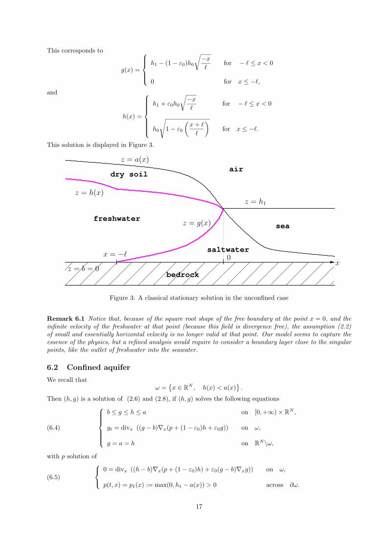
This solution is displayed in Figure 3.

airdry soil

sea

bedrock

freshwater

saltwater

z = a(x)

z = h1

z = h(x)

z = b = 0

z = g(x)

xx = −` 0

Figure 3: A classical stationary solution in the unconfined case

Remark 6.1 Notice that, because of the square root shape of the free boundary at the point x = 0, and theinfinite velocity of the freshwater at that point (because this field is divergence free), the assumption (2.2)of small and essentially horizontal velocity is no longer valid at that point. Our model seems to capture theessence of the physics, but a refined analysis would require to consider a boundary layer close to the singularpoints, like the outlet of freshwater into the seawater.

6.2 Confined aquifer

We recall thatω =

x ∈ RN , h(x) < a(x)

.

Then (h, g) is a solution of (2.6) and (2.8), if (h, g) solves the following equations

(6.4)

b ≤ g ≤ h ≤ a on [0,+∞)× RN ,

gt = divx ((g − b)∇x(p+ (1− ε0)h+ ε0g)) on ω,

g = a = h on RN\ω,

with p solution of

(6.5)

0 = divx ((h− b)∇x(p+ (1− ε0)h) + ε0(g − b)∇xg)) on ω,

p(t, x) = p1(x) := max(0, h1 − a(x)) > 0 across ∂ω.

17

Proposition 6.2 (horizontal confinement)We assume that h ≡ h0 ∈ (0, h1) on ω and b ≡ 0. Then the solution g of (6.4)-(6.5) satisfies for all timest > 0

(6.6)

0 ≤ g ≤ h0 on ω,

g = h0 across ∂ω,

gt = ε0 divx

(g

(1− g

h0

)∇xg

)+ ε0 divx (g∇xβ) on ω,

with β solution of

(6.7)

∆β = 0 on ω,

β =h0

2across ∂ω.

Remark 6.3 The third equation of (6.6) appears to be an approximation of the equation considered in [34],in the limit case where the gradient of the solution is small.

Proof of Proposition 6.2We simply set

β(t, x) = ε−10 (p(t, x)− (h1 − h0)) +

1

2h0g2(t, x).

The end of the proof is straightforward.

Remark 6.4 Because h− b is constant under the confining rock (in ω), notice that

(h− b)∇x(p+ (1− ε0)h) + ε0(g − h)∇xg

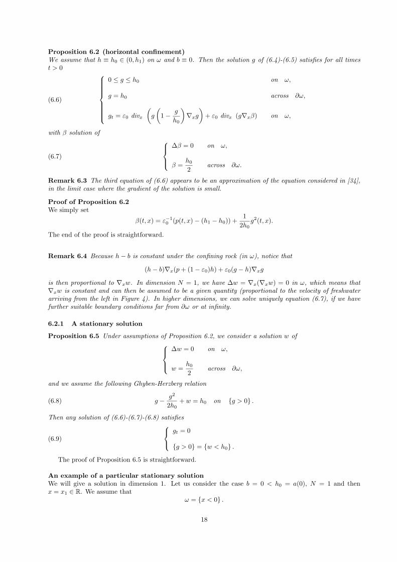
is then proportional to ∇xw. In dimension N = 1, we have ∆w = ∇x(∇xw) = 0 in ω, which means that∇xw is constant and can then be assumed to be a given quantity (proportional to the velocity of freshwaterarriving from the left in Figure 4). In higher dimensions, we can solve uniquely equation (6.7), if we havefurther suitable boundary conditions far from ∂ω or at infinity.

6.2.1 A stationary solution

Proposition 6.5 Under assumptions of Proposition 6.2, we consider a solution w of∆w = 0 on ω,

w =h0

2across ∂ω,

and we assume the following Ghyben-Herzberg relation

(6.8) g − g2

2h0+ w = h0 on g > 0 .

Then any solution of (6.6)-(6.7)-(6.8) satisfies

(6.9)

gt = 0

g > 0 = w < h0 .

The proof of Proposition 6.5 is straightforward.

An example of a particular stationary solutionWe will give a solution in dimension 1. Let us consider the case b = 0 < h0 = a(0), N = 1 and thenx = x1 ∈ R. We assume that

ω = x < 0 .

18

Under the assumptions of Proposition 6.5, for any ` > 0, there exists an explicit solution given by

w(x) =h0

2

(1− x

`

),

and g − g2

2h0+ w = h0 for − ` < x < 0,

g = 0 for x ≤ −`.

This solution is displayed in Figure 4.

air

bedrock

freshwatersaltwater

confining rock

sea

z = a(x)

z = b = 0

z = g(x)

z = h = h0

z = h1

ω

x

x = −`0

Figure 4: A stationary solution in the confined case

AcknowledgmentsThe authors would like to thank A. Al Bitar and R. Ababou for enlighting discussions and for indicationsto the literature on the subject. A discussion with R. Ababou was useful to correct a mistake in a previousversion of the manuscript. The authors also would like to thank A. Fino for helpful discussions, and G.Chmaycem, S. Issa and H. Moustafa for useful remarks on the manuscript. The authors finally thank thetwo unknown referees for their careful reading of the manuscript, their suggestions and numerous correctionsthat helped to improve substantially the presentation of the paper.

References

[1] A. Al Bitar, Modelisation des ecoulements en milieu poreux heterogenes 2D / 3D, avec couplagessurface / souterrain et densitaires, These de l’Institut National Polytechnique de Toulouse, (2007).

[2] G. Alduncin, J. Esquivel-Avila, L. Reyes-Avila, Steady filtration problems with seawater in-trusion: variational analysis, Symposium on Advances in Computational Mechanics, Vol. 3 (Austin,TX, 1997). Comput. Methods Appl. Mech. Engrg. 151 (1-2) (1998), 13–25.

[3] H.W. Alt, C.J. van Duijn, A stationary flow of fresh and salt groundwater in a coastal aquifer,Nonlinear Analysis, Theory, Methods & Applications 14 (8) (1990), 625–656.

[4] M. Bakker, Simple groundwater flow models for seawater intrusion, In: Proceedings of SWIM16,Wolin Island, Poland, (2000).

19

[5] J. Bear, Hydraulics of Groundwater, McGrraw-Hill, New York, (1979).

[6] J. Bear, A.H.D. Cheng, Modeling Groundwater Flow and Contaminant Transport, Theory andapplications of transport in porous media 23, Springer (2010).

[7] J. Bear, A.H.D. Cheng, S. Sorek, D. Ouazar, I. Herrera (Eds.), Seawater Intrusion inCoastal Aquifers - Concepts, Methods and Practices, Theory and applications of transport in porousmedia 14, Kluwer Academic Publisher, Netherlands, (1999).

[8] J. Bear, A. Verruijt, Modelling groundwater flow and pollution, D. Reidel Publishing Company,Dordecht, Holland, (1987).

[9] A. Bonnet, R. Monneau, On the Mushy Region Arising Between Two Fluids in a Porous Medium,Nonlinear Analysis, Real World and Applications 5 (1) (2004), 159–182.

[10] J. Boussinesq, Recherches theoriques sur l’ecoulement des nappes d’eau infiltrees dans le sol et surle debit des sources, Journal de mathematiques pures et appliquees 5eme serie, tome 10 (1904), 5–78.

[11] W.C. Burnett, P.K. Aggarwal, A. Aureli, H. Bokuniewicz, J.E. Cable, M.A. Charette,E. Kontar, S. Krupa, K.M. Kulkarni, A. Loveless, W.S. Moore, J.A. Oberdorfer, J.Oliveira, N. Ozyurt, P. Povinec, 1, A.M.G. Privitera, R. Rajar, R.T. Ramessur, J.Scholten, T. Stieglitz, M. Taniguchi, J.V. Turner, Review: Quantifying submarine ground-water discharge in the coastal zone via multiple methods, Science of The Total Environment 367 (2-3)(2006), 498–543.

[12] Z. Chen, R.E. Ewing, Mathematical analysis for reservoir models, SIAM J. Math. Anal. 30 (1999),431–453.

[13] M. Chipot, Variational inequalities and flow in porous media, Applied Mathematical Sciences, 52.New York etc.: Springer-Verlag, (1984).

[14] H. Darcy, Les fontaines publiques de la ville de Dijon; exposition et application des principes aemployer dans les questions de distribution d’eau. Victor Dalmont, Editeur, Paris, (1856).

[15] J. Dupuit, Etudes theoriques et pratiques sur le mouvement des eaux dans les canaux decouverts eta travers les terrains permeables, 2eme edition, Dunod, Paris, (1863).

[16] M. El Alaoui Talibi, D. Ouazar, M.H. Tber, Identification of the hydraulic conductivities ina saltwater intrusion problem, J. Inverse Ill-Posed Probl. 15 (9) (2007), 935–954.

[17] M. El Alaoui Talibi, M.H. Tber, Existence of solutions for a degenerate seawater intrusionproblem, Electron. J. Differential Equations 72 (2005), 1–14.

[18] H.I. Essaid, A multilayered sharp interface model of coupled freshwater and saltwater flow in acoastal system: Model development and application, Water Ressources Research 26 (7) (1990), 1431–1454.

[19] R. Eymard, R. Herbin, A. Michel, Mathematical study of a petroleum-engineering scheme,ESAIM: Mathematical Modelling and Numerical Analysis 37 (6) (2003), 937–972.

[20] C.W. Fetter Jr, Hydrogeology: A Short History, Part 2, Ground Water, 42 (2004), 949–953.

[21] J.–F. Gerbeau, B. Perthame, Derivation of viscous Saint-Venant system for laminar shallowwater; numerical validation, Discrete and Continuous Dynamical Systems - Series B 1 (1) (2001),89–102.

[22] A. R. Kacimov, Yu. V. Obnosov, Analytical solution for a sharp interface problem in sea waterintrusion into a coastal aquifer, Proc. R. Soc. Lond. A 457 (2001), 3023–3038.

[23] A. R. Kacimov, Yu. V. Obnosov, M. M. Sherif and J. S. Perret, Analytical Solution toa Sea-water Intrusion Problem with a Fresh Water Zone Tapering to a Triple Point, Journal ofEngineering Mathematics 54 (3) (2006), 197–210.

20

[24] C. Kao, Fonctionnement hydraulique des nappes superficielles de fonds de vallees en interaction avecle reseau hydrographique, These de doctorat en Sciences de l’Eau, Ecole Nationale du Genie Rural,des Eaux et Forets (Paris), (2002).

[25] G. Keady, The Dupuit Approximation for the Rectangular Dam Problem, IMA Journal of AppliedMathematics 44 (1990), 243–260.

[26] M. Kemblowski, The Impact of the Dupuit-Forchheimer Approximation on Salt-Water IntrusionSimulation, Ground Water 25 (3) (1987), 331–336.

[27] C.M. Marle, Henry Darcy et les ecoulements de fluides en milieu poreux, Oil & Gas Science andTechnology Rev. IFP, Vol. 61 (5) (2006), 599–609.

[28] P.Y. Polubarinova-Kochina, Theory of Groundwater Movement, translated from Russian edition1952 by R.J.M. De Wiest. Princeton University Press, New Jersey, (1962).

[29] S. Sorek, V. Borisov, A. Yakirevich, A Two-Dimensional Areal Model for Density DependentFlow Regime, Transport in Porous Media 43 (2001), 87–105.

[30] O.D.L. Strack, Groundwater Mechanics, Prentice Hall, Englewood Cliffs, NJ, (1989).

[31] O.D.L. Strack, A Dupuit-Forchheimer model for three-dimensional flow with variable density, Wa-ter Resources Research 31 (12) (1995), 3007–3017.

[32] O.D.L. Strack, R.J. Barnes, A. Verruijt, Vertically Integrated Flows, Discharge Potential,and the Dupuit-Forchheimer Approximation, Special Issue: Ground Water Flow Modeling with theAnalytic Element Method, Ground Water 44 (1) (2006), 72–75.

[33] M.H. Tber, On a seawater intrusion problem, Appl. Sci. 9 (2007), 163–173.

[34] C.J. van Duyn, D. Hilhorst, On a doubly nonlinear diffusion equation in hydrology, Nonlinearanalysis, Theory, Methods and applications 11 (3) (1987), 305–333.

[35] J.L. Vazquez, The porous medium equation: mathematical theory, Oxford University Press, USA,(2007).

[36] E.G. Youngs, An examination of computed steady-state water-table heights in unconfined aquifers:Dupuit-Forchheimer estimates and exact analytical results, J. Hydrol. 119 (1990), 201–214.

21