Embed Size (px)
Citation preview

Department of the TreasuryInternal Revenue Service
Mark W. EversonCommissioner
Mark J. MazurDirector, Research, Analysis, and Statistics
Janice M. HedemannDirector, Office of Research


IRS Research Bulletin
Recent Research on Tax Administration and Compliance
Selected Papers Given at the 2006 IRS Research Conference
Georgetown University School of LawWashington, DCJune 14-15, 2006
Compiled and Edited byJames Dalton and Beth Kilss*Statistics of Income DivisionInternal Revenue Service
*Prepared under the direction of Janet McCubbin, Chief, Special Studies Branch


IRS Research Bulletin iii
ForewordThis edition of the IRS Research Bulletin (Publication 1500) features selected papers from the latest IRS Research Conference, held at the Georgetown Uni-versity School of Law in Washington, DC, on June 14-15, 2006. Conference presenters and attendees included researchers from all areas of IRS, represen-tatives of other government agencies (including from the United Kingdom, Australia, and New Zealand), and academic and private sector experts on tax policy, tax administration, and tax compliance.
The conference began with a keynote address by Mark Matthews, Deputy Commissioner for Services and Enforcement. Mr. Matthews emphasized the importance of using high-quality data and analysis to drive key decisions. Mark Mazur, Director, Research, Analysis and Statistics, then led a panel discus-sion on compliance and administrative aspects of tax reform. The panelists, including former Assistant Secretaries for Tax Policy Pamela Olson and Ronald Pearlman, former Deputy Assistant Secretary for Tax Analysis Leonard Burman, and Jane Gravelle of the Congressional Research Service, emphasized the need to use data and analysis to inform policies as they are first being formulated, rather than after positions have hardened. The remainder of the conference included sessions on corporate compliance, measuring individual compliance, uses of tax data, the role of third parties in tax administration and compliance, and new approaches to compliance administration.
We hope that this volume will enable IRS executives, managers, employ-ees, and stakeholders to stay abreast of the latest trends and research findings affecting Federal tax administration. The research featured here is intended to provide a starting place from which to conduct further analysis.
AcknowledgmentsThis volume was prepared by Paul Bastuscheck and Heather Lilley and edited by James Dalton and Beth Kilss, all of the Statistics of Income Division. The authors of the papers are responsible for their content, and views expressed in these papers do not necessarily represent the views of the Department of the Treasury or the Internal Revenue Service.
IRS Research Bulletiniv
The Conference itself was the result of substantial effort and preparation over a number of months by many people. Melissa Kovalick and Bobbie Vaira arranged for the conference venue, conducted registration and oversaw myriad details to ensure that the Conference ran smoothly. The conference program was assembled by a program committee that represented research groups throughout the IRS. Members of the program committee included Mark Mazur (Director, Office of Research, Analysis and Statistics), Janice Hedemann (Director, Office of Research), Janet McCubbin (Statistics of Income Division), Joel Friedman (Wage and Investment Division), Curt Hopkins (Small Business/Self-Employed Division), Elizabeth Kruse (Office of Program Evaluation and Risk Analysis), Alan Plumley (Office of Research) and David Stanley (Large and Midsize Business Division). We appreciate the contributions of everyone who helped make this Conference a success.
Janice HedemannDirector, Office of Research Janet McCubbinStatistics of Income DivisionCo-chairpersons, 2006 IRS Research ConferenceDecember 2006
Editors’ Note: The papers included in this volume may also be found on the IRS web site at http://www.irs.gov/taxstats/index.html. From this page, click on “Conference Papers” under “Products, Publications, & Papers.” The papers are listed under “IRS Research Conferences: 2006” in alphabetical order by title of session and title of paper.

IRS Research Bulletin v
2006 IRS Research Conference
Contents
Foreword ....................................................................................... iii
1. Corporate Tax Administration and Compliance
v Is the Tax Expense Estimate Improved or Biased in the Presence of Using the Same Tax and Audit Firm?, Cristi A. Gleason and Lillian F. Mills .............................................. 3
v A First Look at the 2004 Schedule M-3 Reporting by Large Corporations, Charles Boynton, Ellen Legel, and Portia DeFilippes ........................................................................... 39
2. Individual Compliance Analysis and Modeling
v Understanding Taxpayer Behavior and Assessing Potential IRS Interventions Using Multiagent Dynamic-Network Simulation, Kathleen M. Carley and Daniel T. Maxwell ................................... 93
v Longitudinal Study of EITC Claimants, Karen Masken .............. 107
3. Uses of Tax Data
v Calibrating Macroeconomic and Microsimulation Models to CBO’s Baseline Projections, Tracy L. Foertsch and Ralph A. Rector ............................................................................ 121
v Tax Variable Imputation in the Current Population Survey, Amy O’Hara ................................................................................. 169

IRS Research Bulletinvi
4. The Role of Third Parties in Tax Administration and Compliance
v Instance-Based Classifiers for Tax Agent Modelling, Fuchun Luan, Warwick Graco, and Mark Norrie ........................ 183
v Tax Filing Experiences and Withholding Preferences of Low- and Moderate-Income Households: Preliminary Evidence from a New Survey, Michael S. Barr and Jane K. Dokko ........... 193
5. New Approaches to Compliance and Administration
v The Effect of Targeted Outreach on Compliance, Peter D. Adelsheim and James L. Zanetti .....................................213
v A New Era of Tax Enforcement: From “Big Stick” to Reponsive Regulation, Sagit Leviner ............................................241
6. Appendix
v Conference Program ......................................................................307
v List of Attendees ...........................................................................311

1
Corporate Tax Administration and Compliance
Gleason u Mills Boynton u Legel u DeFilippes
D

Is the Tax Expense Estimate Improved or Biased
in the Presence of Using the Same Tax and Audit Firm?
Cristi A. Gleason, University of Iowa, and Lillian F. Mills, University of Texas
Regulators have limited firms’ ability to purchase tax services from their audit firms out of concerns that auditors permit biased reporting when their firms provide tax services to their audit clients. Auditor bias
could arise either because of the economic bond generated by the magnitude of the tax services or because a qualitative conflict exists whereby auditors are reviewing the accounting arising from their own firm’s tax advice. On the other hand, providing tax services could improve the estimation of tax expense because the audit firm enjoys knowledge spillover from its tax department. That is, the audit team learns from its tax group more about the tax planning undertaken by the corporation. To date, empirical accounting research in the Sarbanes-Oxley (SOX) period has focused on the possibility that independence is impaired when an audit firm provides tax services to an audit client (Frankel, Johnson, and Nelson, 2002; Antle et al., 2002; DeFond, Raghunandan, and Subramanyan, 2002; Ashbaugh, LaFond, and Mayhew, 2003; Chung and Kal-lapur, 2003; Kinney, Palmrose, and Scholz, 2004; and Larker and Richardson, 2004). Accounting theory, however, provides support for both independence impairment and estimation improvement resulting from audit-provided tax services (Simunic, 1984; Beck, Frecka, and Solomon, 1988). We design tests to distinguish between these competing predictions.
Our study is motivated by the ongoing debate on auditor-provided tax services. The evidence in academic research fails to find lapses in independence for auditor-provided services in general. Also, many commentators advocate permitting tax services because of the benefits of knowledge spillovers. Nev-ertheless, regulators have continued to inhibit tax services provided by auditors beyond the initial restrictions in section 2.01 of the Sarbanes Oxley Act of 2002. The requirement that corporations must obtain audit committee approval for permitted nonaudit services imposes a serious friction that contributes to the decline in auditor-provided tax services (Maydew and Shackelford, 2006). Conservative audit committees are unlikely to approve such tax services based on the current lack of evidence concerning independence failures. In

Gleason and Mills4
the post-SOX climate, saying “no” is safe and easy--saying “yes” requires positive evidence.
Accounting for contingencies related to IRS examinations provides a context in which the differences in competing predictions from audit theory should be especially stark. Firms estimate and record a liability (tax cushion) for the probable and estimable amount of additional tax the firm expects to lose to the IRS as a result of IRS examinations. Determining the amount of tax cushion requires judgment on the part of both management and auditors. The need for judgment provides management with an occasion to record tax benefits or contingencies opportunistically.
Auditors can constrain managers from under- or over-recording tax cushion through their audit procedures. Auditors assess the sufficiency of the tax expense by reviewing tax returns, workpapers, and IRS correspondence to identify areas of tax risk, skeptically evaluating managers’ own risk analysis, seeking outside legal opinions, and conducting tax research to assess the prob-ability of loss.
If an audit firm provides tax planning or tax compliance services, the audit personnel can learn about the existence and technical merits of any uncertain tax positions from the tax personnel. These knowledge spillovers (Simunic, 1984; Beck, Frecka, and Solomon, 1988) can improve the estimation of the probable amount owed. It is more difficult for an audit firm to assess tax risk if its client conducts its own tax planning or uses unrelated consultants. An audit firm that does not provide tax services must first detect aggressive tax positions (or rely on management to reveal those positions), then generate evidence about the expected outcome of those positions.
However, regulators are concerned that nonaudit services impair inde-pendence because substantial services create an economic bond whereby the audit firm does not want to lose a profitable client. The tax setting also has a qualitative effect if the auditor is reviewing the results of its own tax depart-ment’s advice. The potential link between auditor-provided tax services and the impairment of auditor independence is illustrated in the following quote:
The issue of independence is particularly acute when the tax strategy is sold to achieve a particular financial statement result. The whole point of the auditor is to audit the financial statements, but now they’re affecting the financial statement results and they’re then going to audit that? How can that possibly be independent?
Mark Anson (Calpers), PCAOB 2004, p. 111.1
Thus, the alternative to knowledge spillovers is that the auditor permits firms to bias their estimates of tax cushion and thus tax expense. Focusing on the relation between reported tax cushion and deficiency exploits the direct

Is the Tax Expense Estimate Improved or Biased? 5
link between tax planning and tax expense. An underlying assumption is that auditors who do not provide tax services are free from bias. Hence, we use comparisons between firms that do and do not purchase auditor-provided tax services to test for bias or improved estimation of tax cushion.
We analyze observations for years in which the IRS completes its exami-nation. These years represent periods when corporations learn the amount of the disputed tax (the deficiency) and make any concessions by paying some of the disputed tax. Our sample consists of 497 corporation-years with completed examinations and sufficient data from four sources: financial statement data from Standard & Poor’s Compustat, audit fee data from Standard & Poor’s, tax return data, and IRS examination data. The corporations are publicly traded companies in the large- and midsized business (LMSB) division of the IRS. The sample includes years 2000, 2001, and 2002, because auditor fee data were not available until 2000, and because IRS tax data are available to one of the authors only through 2002.
We estimate a regression of tax expense on IRS deficiencies. We expect deficiencies to contribute positively to tax expense.2 This result would occur if firms accrued less than the eventual loss from the deficiency, perhaps because they record the lower amount of a probable range of loss from any tax deficiency (FIN 14). To test whether auditor-provided tax services affect the association between tax expense and tax deficiency, we interact a dummy variable for such services with deficiency in the regression specification.3
We find that only corporations whose auditors do not perform tax services record additional tax expense for the deficiency. Specifically, these corpora-tions increase tax expense by about 78 percent of the deficiency in the year the IRS exam is completed. In contrast, the coefficient for the interaction between deficiency and using auditor-provided tax services is negative, and the net co-efficient is not significantly different from zero. This means that, on average, corporations whose auditors provide tax services do not increase tax expense in response to the IRS deficiency, a result consistent with better estimation of contingent IRS exam liabilities in prior periods. We repeat the analysis using the amount of total payments in settlement with the IRS after all appeals and litigation steps are concluded as the dependent variable, and find that corpo-rations using auditor-provided tax services still do not record additional tax expense. This corroborates our interpretation that these corporations have fully accrued the tax liability prior to the deficiency. We infer that corporations using auditor-provided tax services have adequately, or even conservatively, recorded reserves for tax loss contingencies prior to IRS examination. In other words, these corporations convey bad news sooner to shareholders.
To conclude that recording enough expense for the contingency does not itself lead to earnings manipulation, we investigate whether corporations using auditor-provided tax services overaccrue tax expense to manage earnings. We

Gleason and Mills6
find no association between the presence of auditor-provided tax services and the management of tax expense to meet or beat analysts’ quarterly earnings-per-share forecasts or to smooth earnings. We conclude that purchasing tax services from the auditor does not permit corporations to manage earnings more easily than corporations whose auditors do not provide tax services.
In summary, we find no evidence that providing tax services impairs an auditor’s independence. In contrast, our evidence is consistent with knowledge spillovers from auditor-provided tax services improving the precision of tax cushion estimates, and hence audit quality.
Institutional Background and PredictionsCorporations often pay less tax on their return than will be ultimately required by the IRS after it examines the return and all disputes are settled. Determining how much more will be paid is difficult and requires judgment. Thus, tax loss contingencies present a useful setting to explore whether tax expense estimation is improved or biased for corporations that use the same tax and audit firm.
Estimates of Tax Loss ContingencyTax “cushion” is the term used to describe amounts firms record for contin-gent tax liabilities in anticipation of IRS challenges of uncertain tax positions. SFAS 5 requires that a corporation record the amount of contingent liability that is probable and estimable.4 In applying this standard to contingent tax li-abilities, anecdotal evidence suggests that companies assess the probability of the loss taking into account some or all of the following risks: the risk of the legal uncertainty, the risk of IRS examination, the risk of detection, and the risk of litigation.5 Corporations update their estimates of the tax loss contingency beginning in the fiscal year of the return and extending to the final settlement with the IRS.6
Under SFAS 5, a corporation accrues a loss contingency when the loss is probable and estimable. As a result, corporations would generally record less than the expected value of all losses, because some contingencies that are not judged probable under SFAS 5 would nonetheless occasionally result in a real-ized loss. Further, SFAS 5 states that, when the corporation can only estimate a range, and when no amount in the range is more probable than any other, the corporation should record the bottom number in the range. Conditional on the same expected value, a more precise estimate results in a higher lower bound. Therefore, a more precise estimate results in a higher accrual if firms book the bottom number in the range.
Coupled with difficulties in estimating tax cushion, managers face in-centives to bias earnings estimates to achieve financial reporting objectives.

Is the Tax Expense Estimate Improved or Biased? 7
Managers may record lower amounts of cushion in order to meet bonus targets, debt covenants, or analyst earnings targets. Alternatively, managers may record excess cushion to build a “cookie jar,” with the intent to smooth earnings now and provide flexibility to meet targets in the future.
Role of AuditorsWe assume that independent auditors require corporations to make objective unbiased accounting reports (Ashbaugh, Lafond, and Mahew, 2003). Thus, if managers underreport loss contingencies or conservatively report contingen-cies and use that conservatism for earnings smoothing, we would interpret such reporting as opportunistic bias. Such bias would appear consistent with an independence failure. With respect to the precision of managers’ cushion estimates, auditors may improve the estimate. This improvement comes from greater experience and expertise than are available inside the firm. When the auditor also provides nonaudit services, there is the potential for “knowledge spillovers” (Simunic, 1984; Beck, Frecka, and Solomon, 1988).
Theory offers contradictory explanations for how nonaudit services affect the quality of the audit with respect to bias. Nonaudit services may improve audit quality in two ways. First, knowledge spillover should reduce the bias of contingency estimates because auditors are more familiar with the tax treat-ment. Second, nonaudit services may increase the costs to the auditor of a potential audit failure due to increased litigation risk and reputation concerns (Reynolds and Francis, 2001), motivating auditors to higher skepticism and increased scrutiny.
Knowledge spillover should increase the precision of tax contingency estimates because auditors who also provide tax planning or compliance ser-vices already know about the existence of tax positions that create uncertain tax benefits. They should also have superior information about the probable outcome of those tax plans, because they already know how well the client’s fact patterns and legal structures match the requirements of any tax precedents. Participants in the PCAOB Roundtable discussion express this view as follows: “I do think the fundamental provision of tax services does, in fact, enhance the audit process” (Lynn Turner (Glass Lewis, former chief accountant SEC), PCAOB Roundtable 2004, p. 23). “We also believe that the provision of tax advice… [for] public registrants serves the public interest by permitting the auditor to conduct an efficient audit in respect to tax matters” (Mr. Brasher (KPMG), PCAOB 2004, p. 28).
Holding the expected value constant, the lower bound on a more precise estimate will be higher, so that the auditor will require the corporation to record more tax cushion. Thus, absent any bias, corporations using auditor-provided tax services should record higher amounts of tax cushion prior to learning the

Gleason and Mills8
amount of the deficiency or settlement than other corporations, if knowledge spillovers from providing tax services enhance the audit.
Alternatively, nonaudit services may decrease audit quality by permitting bias in cushion. The audit firm’s dependence on the nonaudit service revenue may increase the economic bond between the auditor and client and decrease the likelihood the auditor corrects any bias (Beck, Frecka, and Solomon, 1988; Kinney and Libby, 2002). The bond between the auditor and client has a qualitative as well as economic aspect if the nonaudit service is tax advice that directly affects earnings:
If you get … that aggressive recommendation from the tax depart-ment of the audit firm, how likely is the auditor to call that advice into question? … When push comes to shove, will the auditor call that recommendation into question? And I think that becomes significantly less likely if the recommendation came from his own firm.
Barbara Roper (Consumer Federation of America), PCAOB Roundtable 2004, p.80.
Because there are widely held but conflicting predictions regarding the ef-fect of auditor-provided tax services on auditor independence versus knowledge spillover, we examine the issue empirically.7 We focus on tax contingencies for IRS examination deficiencies. We state our research question as follows:
RQ1: Do corporations whose auditors provide tax services record higher, lower, or equivalent amounts of tax expense for tax loss contingencies compared with corporations whose auditors do not provide tax services?
Managers’ reporting incentives could create bias in either direction: delaying or accelerating the recording of cushion. If auditor-provided tax services are associated with insufficient amounts of cushion, we will conclude that such auditors permit managers to manage earnings upward by recording less tax cushion.
However, if auditor-provided tax services are associated with higher amounts of cushion, we cannot distinguish better estimation from opportunism merely based on the amounts of recorded cushion. To distinguish improved precision from opportunistic overaccrual (cookie jar), we consider whether auditor-provided tax services are associated with earnings management. We investigate the following additional research question:
RQ2: Do corporations whose auditors provide tax services manage earnings via tax expense more frequently than those who do not?

Is the Tax Expense Estimate Improved or Biased? 9
Research DesignTo answer the first research question, we estimate a regression model of tax expense on tax deficiency. We interact the tax deficiency with a dummy variable for auditor-provided tax services to investigate whether the amount of deficiency recorded in tax expense is higher or lower in the presence of using the same tax and audit firm. For the impact on tax expense, we use two measures: tax cushion and the U.S. current tax expense.
Cushionit or U.S. Current Taxit = a0 + a1Tax&Auditit + a2Tax&Auditit* Deficiencyit + a3 Deficiencyit + (a4US Tax Paidit + a5Option Tax Benefitit)+ a6Log(Sales)it +a7Propertyit + a8R&Dit + a9Foreignit + Yearit + eit,where
Cushion = U.S. Current Tax Expense (Compustat item #63, or #16-#50 if missing) less unscaled Option Tax Benefit less unscaled U.S. Tax Paid, divided by pretax income (#170).
U.S. Current Tax = U.S. current tax expense (#63), divided by pretax income.
Tax&Audit = 1 if the audit firm also performs tax services, zero otherwise.Deficiency = sum of proposed deficiencies for examinations of post-1989
return-years that were completed during the current year, divided by pretax income in the current year.
(U.S. Tax Paid) = Tax After Credits from the U.S. tax return, divided by pretax income.
(Option Tax Benefit) = the tax benefit from stock options disclosed in the statement of cash flows or statement of stockholders’ equity. Where the amount is not disclosed, we compute the Option Tax Benefit to equal 35 percent times the number of share exercised times the difference between the average stock price for the year and the average exercise price. If the latter computation is negative, we use the maximum stock price for the year in place of the average stock price. Finally, we set the benefit to zero where it is missing or nega-tive.
Log(Sales) = Log of millions of dollars of sales (#12). Property = Net property plant and equipment (#8) divided by assets (#6).R&D = Research and Development Expense (#46 if nonmissing, otherwise
zero) divided by sales.Foreign = absolute value of [foreign pretax income (#273 if nonmissing,
zero otherwise) divided by pretax income].

Gleason and Mills10
Our main dependent variable is a direct measure of U.S. tax cushion (Cushion) that builds on Gleason and Mills, 2002. We measure Cushion as U.S. current tax expense minus unscaled Option Tax Benefit minus unscaled U.S. Tax Paid, divided by pretax income. Although Cushion estimates the additional U.S. current tax payable due to contingent tax liabilities, it may not relate directly to net earnings. Increases and decreases in Cushion could arise due to imprecision in the corporation’s determination of U.S. Tax Paid (because corporations generally do not finalize their tax returns until 8 months after each fiscal yearend) or due to reclassifications from deferred taxes.8 As an alterna-tive to using Cushion, we use U.S. Current Tax and control for U.S. Tax Paid and Option Tax Benefit. Our dependent variables are subject to measurement error because they are adjusted for corrections of estimates related to refund claims, estimated taxes, and other payments that were not recorded in current expense in prior years.
Deficiency is the additional amount of tax the IRS proposes when it com-pletes its examination. We construct Deficiency by summing all deficiencies related to examinations completed during the financial reporting year, divided by pretax income. Our sample uses only financial reporting years during which the IRS completes an exam and the taxpayer learns the result of the examina-tion. Thus, the corporation receives new information about the contingent tax liability during that year.9
Tax&Audit * Deficiency is our main variable of interest. If having the same provider for tax and audit services results in different amounts being recorded in tax expense for a given amount disputed by the IRS, the coeffi-cient will be different from zero. An insignificant interaction term indicates a lack of evidence that corporations are more or less conservative in recording income tax expense when they purchase tax services from their auditors than when they do not.
Where U.S. Current Tax is the dependent variable, we also include con-trols (U.S. Tax Paid, Option Tax Benefit,) for taxes paid and the tax benefit of stock option deductions. The stock option tax benefit is directly recorded in stockholders equity and thus affects U.S. Tax Paid but not Tax Expense (Hanlon and Shevlin, 2002). All of the tax components are scaled by pretax income. We top- and bottom-code the U.S. Current Tax effective tax rate at 1 percent and 0 percent, following Gupta and Newberry, 1997.10
We include several control variables that are related to tax planning and effective tax rates in prior research (Gupta and Newberry, 1997; Mills, Erickson, and Maydew, 1998). Property, Inventory, R&D, and Leverage are defined as in Gupta and Newberry, 1997. Mills et al., 1998 use compliance costs survey data to construct Foreign and Log(Sales); here, we use Compustat data to construct similar measures.

Is the Tax Expense Estimate Improved or Biased? 11
If larger corporations have more opportunity and sophistication to con-duct tax planning, they will pay less tax (Mills et al., 1998), but, if they face higher political costs, then size could be positively related to tax payments (Zimmerman, 1983). Conditional on taxes paid on the return, if large corpo-rations expect to prevail more frequently against the IRS, they would record less tax cushion.
We include capital assets (Property) to control for the portion of the deficiency related to temporary differences that should not affect earnings. Including Property controls for the possibility that Tax&Audit firms perform tax planning that generates Deficiencies arising from temporary rather than permanent differences.
Intellectual property and foreign operations should be associated with lower tax expense through credits and opportunities for tax-motivated income shifting to low-tax jurisdictions (Grubert and Slemrod, 1998; Mills and New-berry, 2004). We use R&D expense scaled by sales (R&D) and the absolute value of the ratio of foreign pretax income to total pretax income (Foreign) to proxy for these income-shifting opportunities. Although the IRS is aware of these tax planning opportunities, the tax laws concerning cost-sharing, valuation, and other aspects of income-shifting are difficult to enforce. Thus, corporations may not need to record as much tax cushion for tax planning related to intangibles, holding tax payments, and deficiencies constant.
We include year controls for time-specific economic or tax law changes. To deal with the sample dependence problem, we report Huber-White robust standard errors (Rogers, 1993, generalizing White, 1980). The maximum- likelihood estimation procedure assumes and estimates a common component of the variance and covariance matrix for all observations from the same corpora-tion. The standard errors are robust to heteroskedasticity and serial correlation (StataCorp, 1999, p. 257). Our results are qualitatively unchanged if we use an industry control instead of clustering by corporation.
To provide evidence on our second research question, we test whether earnings management is more frequent among firms with auditor-provided tax services. We extend Dhaliwal, Gleason, and Mills, 2004 to consider whether corporations with auditor-provided tax services more frequently achieve analysts’ targets using tax expense. We also test for differences in earnings smoothing using tax expense.
We do not test whether nonaudit services affect nontax accounts such as discretionary accruals because prior literature has already extensively exam-ined this setting. Thus, we do not investigate whether Tax&Audit firms permit earnings management in other accounts.
Gleason and Mills12
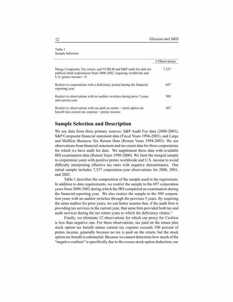
Table 1 Sample Selection
# Observations
Merge Compustat, Tax return, and VCBLM and S&P audit fee data for publicly-held corporations from 2000-2002, requiring worldwide and U.S. pretax income > 0.
7,337
Restrict to corporations with a deficiency posted during the financial reporting year.
697
Restrict to observations with no auditor switches during prior 5 years and current year.
509
Restrict to observations with tax paid on return + stock option tax benefit less current tax expense < pretax income.
497
Sample Selection and DescriptionWe use data from three primary sources: S&P Audit Fee data (2000-2003), S&P Compustat financial statement data (Fiscal Years 1994-2003), and Large and MidSize Business Tax Return Data (Return Years 1994-2003). We use observations from financial statement and tax return data for those corporations for which we have audit fee data. We supplement these data with available IRS examination data (Return Years 1990-2000). We limit the merged sample to corporation years with positive pretax worldwide and U.S. income to avoid difficulty interpreting effective tax rates with negative denominators. Our initial sample includes 7,337 corporation-year observations for 2000, 2001, and 2002.
Table 1 describes the composition of the sample used in the regressions. In addition to data requirements, we restrict the sample to the 697 corporation years from 2000-2002 during which the IRS completed an examination during the financial-reporting year. We also restrict the sample to the 509 corpora-tion years with no auditor switches through the previous 5 years. By requiring the same auditor for prior years, we can better assume that, if the audit firm is providing tax services in the current year, that same firm provided both tax and audit services during the tax return years to which the deficiency relates.11
Finally, we eliminate 12 observations for which our proxy for Cushion is less than negative one. For these observations, tax paid on the return plus stock option tax benefit minus current tax expense exceeds 100 percent of pretax income, generally because no tax is paid on the return, but the stock option tax benefit is substantial. Because we cannot determine how much of the “negative cushion” is specifically due to the excess stock option deduction, our

Is the Tax Expense Estimate Improved or Biased? 13
measure of Cushion is skewed for such firms. Thus, we use the sample of 497 that excludes these 12 observations for our tabulated results. The regression results are qualitatively similar if we include the 12 observations with cushion less than negative one. Results are also robust to further limiting the sample to exclude all firms with zero taxes paid on the U.S. return (sample n=439). We winsorize the continuous variables at 1 percent and 99 percent.
Table 2 describes our dependent and independent variables for the sample. Average Worldwide Tax Expense is 36.6 percent, consistent with Federal, for-eign, and State statutory rates. Mean and median Cushion are both positive, consistent with U.S. Current Tax less Option Tax Benefit, generally exceeding
Table 2 Descriptive Statistics for the sample of corporation-year observations from 2000-2002with audit fee, tax return, IRS examination, and financial statement data
Variable N Mean Std Dev Q1 Median Q3
Tax expense variables
Cushion 497 0.022 0.160 -0.022 0.011 0.057U.S. Current Tax 497 0.247 0.185 0.123 0.244 0.326Worldwide Tax Expense 497 0.366 0.110 0.328 0.364 0.394U.S. Tax Expense U.S. Tax Paid 497 0.182 0.163 0.048 0.165 0.272Option Tax Benefit 497 0.041 0.088 0.002 0.011 0.038
Fee variables Tax&Audit 497 0.579 0.494 0.000 1.000 1.000TaxAuditRatio 497 0.260 0.531 0.000 0.000 0.263Log(TaxFees) 497 1.881 2.875 0.000 0.000 4.605Log(TotalFees) 497 7.110 1.378 6.098 7.041 8.062Log(NonauditFees) 497 6.027 2.139 4.905 6.219 7.513Log(1+TaxFee/SGA) 412 0.001 0.002 0.000 0.000 0.000 IRS Examination variables Deficiency 497 0.033 0.093 0.000 0.004 0.023Paid at Exam 497 0.020 0.055 0.000 0.002 0.014Settlement 391 0.019 0.047 0.000 0.002 0.014Settlement Ratio 480 0.536 1.383 0.222 0.500 0.800
Other variables Log(Sales) 497 7.047 1.702 5.857 7.122 8.195Property 497 0.319 0.227 0.144 0.272 0.445R&D 497 0.021 0.047 0.000 0.000 0.017Foreign 497 0.140 0.242 0.000 0.000 0.204a See Appendix for variable definitions.

Gleason and Mills14
U.S. Tax Paid in the years in which the IRS completes an examination. Fifty-eight percent of the observations use the same tax and audit firm.12 Tax fees represent about 26 percent of audit fees on average. Average Deficiency of 3.3 percent of pretax income exceeds the third quartile, indicating that Deficiency is skewed, with many corporations having small or zero deficiencies. Our sample corporations are large, consistent with a high likelihood of IRS audit.13 The settlement ratio is 53.6 percent with a large standard deviation, arising from some negative settlements (IRS issues a refund after claims) or settlements in excess of 100 percent. Because the settlement ratio is not a regression vari-able, we do not trim or delete these outliers, although our results are robust to dropping these observations. Net depreciable property comprises 32 percent of
Table 3 Correlation and Tests of Differences in Means
Panel A: Correlations of tax measures with explanatory and control variables (N=497)
Cushion U.S. Current Tax Deficiency 0.27721 0.21043
<.0001 <.0001
Paid at Exam 0.18845 0.12475 <.0001 0.0054
Settlement 0.25234 0.13353 N=391 <.0001 0.0082
Tax&Audit -0.12458 -0.06674 0.0054 0.1373
TaxAuditRatio 0.00728 0.00533 0.8714 0.9056
Log(Sales) 0.07854 0.11633 0.0802 0.0094
Property -0.02437 -0.12598 0.5879 0.0049
R&D -0.0849 -0.01552 0.0586 0.7301
Foreign 0.05154 0.27784 0.2515 <.0001
a See Appendix for variable definitions.

Is the Tax Expense Estimate Improved or Biased? 15
assets. Research and development expenses are 2.1 percent of sales, and foreign pretax income is 14 percent of worldwide pretax income in absolute value.
Table 3 provides univariate tests, including correlations of dependent with independent variables and t-tests of mean differences. Deficiency, Paid at Exam, and Settlement are positively correlated with Cushion and U.S. Current Tax, consistent with current tax expense, including not only taxes paid but also the probable loss on contingent liabilities.
Tax&Audit is not correlated with U.S. Current Tax but is negatively cor-related with Tax Cushion. The ratio of auditor-provided tax fees to audit fees is uncorrelated with Cushion or U.S. Current Tax. Log(Sales) is positively cor-related with U.S. Current Tax but only weakly correlated with Cushion. R&D is negatively correlated with Cushion. Foreign is positively correlated with U.S. Current Tax, and Property is negatively correlated with U.S. Current Tax.
In Panel B of Table 3, we consider how effective tax rates and other variables differ depending on whether the corporation does or does not hire
Table 3 Correlation and Tests of Differences in Means
Panel B: Differences in means
Variable a Mean for Same Tax&Audit
N=288
Mean for Different Tax&Audit
N=209
t-statistic Difference in Means
Cushion 0.005 0.046 2.71***
U.S. Current Tax 0.283 0.312 1.45
Worldwide Tax Expense 0.349 0.356 1.25
U.S. Tax Expense 0.320 0.347 1.82*
U.S. Tax Paid 0.180 0.185 0.12
Option Tax Benefit 0.040 0.043 0.28
Deficiency 0.032 0.034 0.32
Paid at Exam 0.020 0.021 0.29
Settlement 0.017 0.021 0.63
Settlement Ratio 0.608 0.440 -1.40
Log(Sales) 7.134 6.937 -1.29
Property 0.310 0.332 0.64
R&D 0.023 0.019 -1.50
Foreign 0.141 0.139 -0.30
***, **, * significant at 0.01, 0.05, 0.10 a See Appendix for variable definitions.

Gleason and Mills16
its audit firm to perform tax services. Using the same tax and audit firm is associated with lower Cushion and U.S. Tax Expense. However, using the same tax and audit firm does not result in lower Worldwide Tax Expense, U.S. Current Tax, or U.S. Tax Paid. Thus, we find no univariate evidence that audi-tor-provided tax services are more effective than nonauditor services for tax planning, which could include consulting by nonauditor CPA firms, lawyers, and inhouse expertise.14
We find no evidence that using the same tax and audit firm reduces deficiencies, amounts PaidAtExam, settlements, or the percent of deficiency that is settled. Finding no differences in examination outcomes between the groups suggests that any differences in Tax Expense or Cushion in the regres-sion results to follow are not due to underlying differences in examination outcomes. Finally, there are no differences in size, capital intensity, R&D, or foreign income percent.
Regression ResultsTable 4 reports results of estimating our regression model to test our first re-search question and to provide partial evidence concerning our second research question. Cushion and U.S. Current Tax are significantly (p<0.001) positively related to Deficiency. This main effect shows that corporations record additional tax expense when they do not use auditor-provided tax services.
Based on the significant negative interaction of Tax&Audit*Deficiency, corporations that use auditor-provided tax services record less tax deficiency in tax expense in the year the IRS completes its examinations. Untabulated F tests show that the net coefficients on Deficiency for corporations with the same tax and audit firm (Tax&Audit * Deficiency + Deficiency) are not significantly different from zero. Thus, corporations using the same tax and audit firm do not record more tax expense when the IRS proposes a deficiency.
We use the dummy variable because the textual description of auditor-provided tax services in 2000 and 2001 often mentions the presence of tax consulting without disclosing the amount of the fee. Thus, we believe our dummy variable better measures the presence of auditor-provided tax services. In robustness tests, we use the ratio of tax fees to total audit fees (audit fees and audit-related fees) or a dummy variable for this ratio being in the upper quartile in place of a dummy variable for the presence of auditor-provided tax services. Results from substituting a continuous explanatory variable are mixed, possibly because we necessarily assign zero to observations where the text description mentions the presence of tax services.15
Because it is possible that some corporations record reserves in deferred tax expense during our sample period, we introduce U.S. Deferred Tax Expense as a control in a robustness test. Specifically, if we include U.S. deferred income

Is the Tax Expense Estimate Improved or Biased? 17
tax expense scaled by pretax income in the Cushion regression, the coefficient on U.S. Deferred Tax Expense is significantly negative, and the coefficient on the Deficiency variable is about 0.7. Thus, it appears that some of the increase to Cushion is a reclassification from deferred tax payable to current tax pay-able. Regardless, our conclusion is unchanged: corporations that do not use their auditors for tax services record additional tax cushion, but corporations that use their auditors for tax services do not record additional tax cushion.
Table 4 Regressions of U.S. tax cushion or U.S. current tax expense on IRS deficiencies, testing interaction with presence of auditor-provided tax services
Variable a Cushion U.S. Current Tax
Predicted SignCoefficientt-statistic
Coefficientt-statistic
Intercept 0.0000 0.0973 0.00 3.09
Tax&Audit 0.0008 -0.0025 0.06 -0.22
Tax&Audit * Deficiency - -1.1606 -0.8246
-6.22 -3.53 Deficiency + 1.0375 0.7831
9.95 3.48 U.S. Tax Paid n/a 0.7502
12.91 Option Tax Benefit n/a 0.2774
2.31 Log(Sales) 0.0027 0.0040
0.78 1.29 Property -0.0370 -0.0944
-1.47 -3.78 R&D -0.2637 -0.1035
-1.53 -0.72 Foreign 0.0490 -0.0242
1.27 -0.88 Year Not reported
R-squared 21% 62% # Observations 497 497 a See Appendix for variable definitions. b Robust standard errors were computed using Huber-White corrections with clustering on employer identification number (StataCorp, 1999).

Gleason and Mills18
Control variables are consistent with the composition of effective tax rates. Current tax expense is positively related to the noncushion components of U.S. Tax Paid and Option Tax Benefit.16 As expected, Property is associated with lower current tax expense.
An alternative explanation for the negative interaction coefficient on Deficiency is that corporations using auditor-provided tax services postpone recording the tax cushion until after the year the IRS completes its examina-tion (when we measure Deficiency). If so, our interpretation that Tax&Audit firms are adequately provided when the IRS completes its examination would be incorrect.
In untabulated tests, we consider whether Tax&Audit firms record tax contingencies prior to the year the IRS completes its examination. In place of Deficiency, we use the amount of the deficiency that the corporation pays (Paid at Exam) rather than appealing. Paid at Exam equals the sum of all payments related to examinations finished during the financial reporting year, scaled by pretax income. Paid at Exam represents the minimum tax dispute lost because the corporation concedes this amount.17 The corporation must fully accrue taxes Paid at Exam before or during the fiscal year to equal the credit to cash. Using this measure also eliminates differences across corporations in the likelihood of prevailing. Our results are qualitatively similar to Table 4. The coefficients relating either Cushion or U.S. Current Tax to PaidAtExam are nearly 1, sug-gesting that corporations that do not use the same tax and audit firm have pre-viously recorded little of the amount they concede on examination. Consistent with Table 4, each interaction coefficient is negative and significant, and the net coefficient is not different from zero. Thus, corporations using the same tax and audit firm do not record additional tax expense even for payments that they make at examination, suggesting their reserve was adequate in advance of any payment.
In Table 5, we test whether corporations postpone recording tax contin-gencies until the year of final settlement. To distinguish between the possibili-ties that Tax&Audit firms postpone recognition of contingencies and that they record more cushion prior to learning the Deficiency, we examine the relation between Tax Expense and Settlement. Because the taxpayer can make partial payments during the examination, appeals, or counsel process, Settlement is a noisy measure of new information during the year the return closes.
Results in Table 5 suggest that when the return year closes, firms generally record additional Cushion and U.S. Current Tax. The coefficients on Settle-ment are not significantly different from 1. As in the Deficiency regression, if we introduce U.S. Deferred Tax as a control variable in untabulated tests, the coefficient on Settlement in the Cushion regression decreases to 0.93.

Is the Tax Expense Estimate Improved or Biased? 19
The coefficient on Tax&Audit * Settlement is significantly negative in both regressions, and untabulated F-tests indicate that the net of the main ef-fect and the interaction term is not different from zero. Thus, corporations that use auditor-provided tax services need not record additional expense when the return closes.
One concern is that there is an endogenous relation between purchasing tax services from the auditor and IRS audit deficiencies. We explicitly test whether OLS estimates are consistent with those generated by an instrumental
Table 5 Regressions of tax expense or U.S. tax cushion on settlements of IRS examinations, testing interaction with presence of auditor-provided tax services
Variable a Cushion U.S. Current Tax Coefficientt-statistic
Coefficientt-statistic
Intercept -0.0010 0.0832 -0.03 2.26
Tax&Audit 0.0087 0.0112 0.55 0.88
Tax&Audit * Settlement -1.2024 -1.1965
-1.91 -2.21 Settlement 1.4062 1.2073
3.05 2.38 U.S. Tax Paid n/a 0.8058
15.66 Option Tax Benefit n/a 0.3786
3.52 Log(Sales) -0.0020 0.0007
-0.48 0.18 Property -0.0285 -0.0661
-1.14 -2.92 R&D -0.4436 -0.2255
-1.93 -1.30 Foreign 0.0237 -0.0420
0.60 -1.86 Year Not reported Not reported
R-squared 12% 63% # Observations 391 391
a See Appendix for variable definitions. b Robust standard errors were computed using Huber-White corrections with clustering on employer identification number (StataCorp, 1999).

Gleason and Mills20
variables approach using an augmented regression test suggested by Davidson and MacKinnon, 1993. The Davidson and MacKinnon test is a general endo-geneity test appropriate where heteroskedasticity or serial correlation is pres-ent in the error term. This test of endogeneity requires us to identify variables that are likely associated with the probability of a firm purchasing tax services from the auditor. Prior studies (Antle, 2002; Omer, Bedard, and Falsetta, 2006a; and Omer, Bedard, and Falsetta, 2006b) estimate nonaudit or tax fees as part of two-stage estimations to predict nonaudit or tax fees using variables such as firm size, foreign operations, log of statement of cash flow taxes paid, leverage (agency), quick ratio (risk), book-to-market ratio (risk), whether the firm reports negative net income (risk), audit firm tenure, qualified opinions (risk),and whether the audit firm is one of the “Big 4.” A limitation of many of these variables is that they are likely to be associated with the more general need for externally provided tax services, rather than the specific decision to acquire these services from the audit firm.18
For firms that need outside tax services, a number of factors may affect the decision to purchase tax services from their auditors. First, firms that frequently challenge IRS deficiencies are likely to benefit from the attorney-client privilege and thus are more likely to purchase services from an attorney rather than the auditor. We use the IRS examination data to construct a measure (Combative) of the average percentage of deficiency that the taxpayer decides to appeal. Finally, firms with option plans are more likely to use the auditor for executive tax services because the auditor is already familiar with the option plan and can provide tax services more efficiently. We use Execucomp data to measure the proportion of executive compensation related to stock option value.19 Requiring Execucomp data shrinks our sample to 270 observations. Our tests for endogene-ity are insignificant when either U.S. Current Tax or Cushion is the dependent variable. Nevertheless, we reestimate our regressions using an instrumental variables approach because Greene, 2003 indicates that endogeneity may be a problem even when tests are negative. We add OptionPct and Combative to the instruments used by Omer, Bedard, and Falsetta, 2006 and Antle et al., 2002. Our results are robust to including controls for endogeneity.20
Tests of Earnings ManagementWe triangulate our results on the recording of tax expense with evidence on earnings management. We test whether corporations more frequently beat benchmarks or smooth earnings using tax expense if they engage their audi-tors to provide tax services. Gleason and Mills, 2006 and Dhaliwal, Gleason, and Mills, 2004 together find that the discontinuity around beating analysts’ annual earnings forecasts is explained in part by corporations decreasing tax

Is the Tax Expense Estimate Improved or Biased? 21
expense to beat the forecast. We focus on incentives to meet analysts’ forecast benchmarks because they are relevant for the large publicly traded firms that comprise our sample (Brown and Caylor, 2005). Likewise, incentives to smooth earnings are present for broad samples of firms. Thus, these settings allow us to test for fine degrees of earnings management in our sample.
We use quarterly data from Compustat and I/B/E/S to construct a measure (Tax_Beat) of whether a decrease in the effective tax rate from the prior quarter permitted the corporation to beat analysts’ forecasts. We include only quar-ters two through four in our tests, following evidence in Comprix, Mills, and Schmidt, 2006 that firm behavior is substantially different in the first quarter.
We conduct chi-square tests of whether the proportion of corporations for which Tax&Audit =1 and decreases in tax expense permit them to beat the forecast is greater than the proportion of corporations that do not use auditor-provided tax services (Tax&Audit = 0) and beat the forecast due to a decrease in tax expense.
In Table 6, Panel A, we report results for the full sample and by quarter for the period from 1994-2003. We consider years before and after the year of deficiency to observe whether management behavior differs leading up to the IRS exam and after its conclusion. We include observations from quarters two through four in our test if actual and pretax-managed earnings are within 5 cents of the consensus analyst forecast, where pretax-managed earnings are earnings using the effective tax rate from the prior quarter. Firms within 5 cents of the earnings target are more likely to be able to use tax expense to achieve the target.21
We find that there is no difference between the Tax&Audit groups in the proportion of firms beating the consensus forecast via a decrease in tax expense. Untabulated results by year show a similar pattern of no significant difference between Tax&Audit groups. We also observe that the fraction of the firms beat-ing the target via a decrease in tax expense is larger than the fraction of firms missing the forecast only in the fourth quarter. This is consistent with evidence in Jacob and Jorgensen, 2005 and Das and Shroff, 2002 that firms appear to increase earnings management activities in the fourth quarter.
We also replicate the chi-square tests specifically for the firm-year obser-vations for which the IRS completed an examination. Because Tax&Audit = 1 firms appear to record tax cushion in advance of the examination year, it is possible they have additional slack to beat the analyst target in the examination year. The results reported in Table 6, Panel B are consistent with results in Panel A. Decreasing tax expense during the year to meet or beat analysts’ forecasts is no more frequent for corporations that employ auditor-provided tax services than for corporations that do not use their auditors for tax services.
The results of Table 6 are generally consistent with Omer et al., 2006. They confirm the Dhaliwal, Gleason, and Mills, 2004 result that corporations

Gleason and Mills22
Table 6 Chi-square tests of whether, among corporations that would miss an analyst target absent a decrease in tax expense, corporations using auditor-provided tax services achieve analysts’ earnings targets more frequently Panel A: Exam completion year and pre- and post-period (1994-2003)a
Full Sample Missed consensus Decreased Tax Expense
to beat consensus Column Total
(column%)
Tax&Audit = 0 462
(41%)364
(40%)826
(41%)
Tax&Audit = 1 661
(59%)547
(60%)1208(59%)
Row Total 1123 911 2034 2 = 0.59 (p-value = 0.44)
Second Quarter
Missed consensus Decreased Tax Expense to beat consensus
Column Total (column%)
Tax&Audit = 0 160
(42%)106
(39%)266
(41%)
Tax&Audit = 1 220
(58%)165
(61%)385
(59%)
Row Total 380 271 651 2 = 0.59 (p-value = 0.44)
Third Quarter
Missed consensus Decreased Tax Expense to beat consensus
Column Total (column%)
Tax&Audit = 0 180
(40%)127
(45%)307
(42%)
Tax&Audit = 1 268
(60%)152
(54%)420
(58%)
Row Total 448 279 727 2 = 2.0105 (p-value = 0.16)
Fourth Quarter
Missed consensus Decreased Tax Expense to beat consensus
Column Total (column%)
Tax&Audit = 0 122
(41%)131
(36%)253
(42%)
Tax&Audit = 1 173
(59%)230
(64%)403
(58%)
Row Total 295 361 656 2 = 1.7598 (p-value = 0.18)

Is the Tax Expense Estimate Improved or Biased? 23
that would otherwise miss their analysts’ earnings targets have greater decreases in their fourth quarter effective tax rates than do corporations that would meet the target. Although firms that pay greater fees to their auditors have larger decreases, they also find that corporations that do not engage their auditors for tax services also decrease tax rates to beat earnings. Similar to our tests, they do not find more frequent earnings management among firms that engage their auditors for tax services.
We also test whether corporations for whom Tax&Audit =1 have smoother earnings than other corporations. One possible reason to record higher levels of cushion is to build a “cookie jar” in order to smooth earnings in the cur-rent and subsequent periods. To measure smoothing, we adapt the smoothing measures used by Land and Lang, 2002; Leuz, Nanda, and Wysocki, 2003; Lang, Ready, and Wilson, 2005; and Myers, Myers, and Skinner, 2005. In prior research, smoothing is measured as the degree of negative correlation between the change in discretionary accruals and the change in prediscretion-ary income. In order to focus on the effect of any tax expense management, we measure the correlation between the change in tax-managed earnings and pre-managed income, defined as:
Tax-managed earnings = {pretax earnings per share * (EtrQt-1- EtrQt)}Pretax-managed earnings = {pretax earnings per share * (1-EtrQ3)}
Table 6 Chi-square tests of whether, among corporations that would miss an analyst target absent a decrease in tax expense, corporations using auditor-provided tax services achieve analysts’ earnings targets more frequently Panel A: Exam completion year and pre- and post-period (1994-2003)a
Full Sample Missed consensus Decreased Tax Expense
to beat consensus Column Total
(column%)
Tax&Audit = 0 462
(41%)364
(40%)826
(41%)
Tax&Audit = 1 661
(59%)547
(60%)1208
(59%)
Row Total 1123 911 2034 2 = 0.59 (p-value = 0.44)
Second Quarter
Missed consensus Decreased Tax Expense to beat consensus
Column Total (column%)
Tax&Audit = 0 160
(42%)106
(39%)266
(41%)
Tax&Audit = 1 220
(58%)165
(61%)385
(59%)
Row Total 380 271 651 2 = 0.59 (p-value = 0.44)
Third Quarter
Missed consensus Decreased Tax Expense to beat consensus
Column Total (column%)
Tax&Audit = 0 180
(40%)127
(45%)307
(42%)
Tax&Audit = 1 268
(60%)152
(54%)420
(58%)
Row Total 448 279 727 2 = 2.0105 (p-value = 0.16)
Fourth Quarter
Missed consensus Decreased Tax Expense to beat consensus
Column Total (column%)
Tax&Audit = 0 122
(41%)131
(36%)253
(42%)
Tax&Audit = 1 173
(59%)230
(64%)403
(58%)
Row Total 295 361 656 2 = 1.7598 (p-value = 0.18)
Table 6 Chi-square tests of whether, among corporations that would miss an analyst target absent a decrease in tax expense, corporations using auditor-provided tax services achieve analysts’ earnings targets more frequently--Continued Panel B: Exam completion year only b
Full Sample Missed consensus Decreased Tax Expense
to beat consensus Column Total
(column%)
Tax&Audit = 0 140
(43%)104
(42%)244
(43%)
Tax&Audit = 1 184
(57%)145
(58%)329
(57%)
Row Total 324 249 573 2 = 0.12 (p-value = 0.73)
a Observations for sample firms for quarters two through four in fiscal years between 1994 and 2003 are included if actual and pretax managed earnings are within 5 cents of the consensus analyst forecast. Pretax-managed earnings are defined as earnings computed using the prior quarter’s effective tax rate. b Observations for sample firms for quarters two through four in the fiscal year in which the IRS examination is completed are included if actual and pretax managed earnings are within 5 cents of the consensus analyst forecast.

Gleason and Mills24
We again use quarters two through four and measure the change as the difference between the current quarter and the same quarter of the prior year. We use all quarters from 1994-2005 with available data. Our sample of firms is reduced to 420 corporations with sufficient Compustat data for the test (n = 248 for Tax&Audit =1). In untabulated tests, we find significant negative correlations for corporations for which Tax&Audit =1 (mean ρ = -0.703) and other corporations (mean ρ = -0.701). Individually, the negative correlations are consistent with changes in quarterly effective tax rates helping to smooth earnings.22 However, the difference between the groups is not statistically significant. Thus, the test does not provide any evidence that Tax&Audit =1 corporations smooth earnings via tax expense more than other corporations. Overall, we find no evidence that having the same tax and audit firm is associ-ated with increased occurrence of earnings management or smoothing via tax expense. Therefore, we infer that auditor-provided tax services do not impair independence.
Supplemental Tests Prior research considers other circumstances that may impair auditor indepen-dence. DeAngelo, 1981 suggests that the audit fee can result in an economic bond between the auditor and client that may impair auditor independence. Kinney and Libby, 2002 suggest that the total of audit and nonaudit fees may be an appropriate measure of the economic bond and the potential for impair-ment of auditor independence. We consider both total fees and nonaudit fees other than tax as control variables in robustness tests.
In untabulated tests, we find that our result that Cushion is negatively related to Tax&Audit*Deficiency is robust to including Log (TotalFee) as a main effect and as an interaction with Deficiency. TotalFee is the sum of audit, information systems, tax, and other fees from the S&P database. Our results are qualitatively the same when we use nonaudit fees other than tax as our control variable for economic bond.
The skewed distribution of Deficiency indicates there are some large outliers. Our results are robust to dropping the six observations for which Deficiency exceeds half of pretax income.
The requirement to disclose the tax component of nonaudit services did not take effect until 2002. Although our sample for 2002 alone is quite small (n=41) because we only have tax data through June 2002 fiscal yearends, results are qualitatively the same in this small sample that excludes the volun-tary reporting years. Thus, we conclude that our results are not due to sample selection bias.
We include dummy variables for each of the Big 5 auditors to learn whether amounts accrued differ significantly across firms. Our results are ro-

Is the Tax Expense Estimate Improved or Biased? 25
bust to including dummy variables for each of the Big 5 auditors. We omit this from the tabulation for simplicity because none of the dummies is significantly different from zero.
An alternative explanation for our findings is that, when auditors provide tax services to their audit clients, they recommend tax planning schemes that result in challenges to temporary differences rather than permanent differences and that, in other circumstances, tax planning schemes result primarily in per-manent differences. To the extent the IRS proposes a deficiency related to a permanent item, the claimed tax if lost affects earnings directly. To the extent the deficiency relates to a temporary item, the claimed tax if lost accelerates the payment of tax already recorded in earnings. If Tax&Audit firms have more challenges related to temporary differences, they need not generally record an increase in total tax expense because the Deficiency would affect book earn-ings only through tax penalties and interest expense, which would generally be less than the related tax.
To address potential differences among firms based on relative amounts of permanent and temporary differences, we substitute total TaxExpense, which reflects the net effect of both current and deferred taxes on income, as the dependent variable. Our inferences are unchanged. The smaller coefficient relating Deficiency to total TaxExpense is fully reversed through the negative interaction term. Tax&Audit firms do not record additional total tax payable at the Deficiency date. Recall from Table 3, Panel B that the presence of auditor-provided tax services is not associated with lower tax rates, lower Deficiency, or lower settlement ratios.
The IRS could assess interest and penalties for challenges of both per-manent and temporary differences. FIN 48 suggests that practice concerning classification of interest and penalties varied during our sample period. How-ever, we have no reason to expect that variation in how interest and penalties are classified is correlated with auditor-provided tax services.23 Rather than standardizing practice, the new Interpretation requires that corporations disclose where in the income statement the firm classifies accrued interest and penalties. Future research could explore incentives related to classification once additional data become available.
ConclusionAlthough few auditor-provided tax services were prohibited by Sarbanes Oxley, the requirement to obtain board of directors approval for tax services, and the constraints imposed by the SEC and the PCAOB, have substantially reduced auditor-provided tax services. However, there is no prior evidence that auditor-provided tax services impair independence. Our study focuses on a tax setting where the link between the nonaudit services and financial reporting choices is

Gleason and Mills26
closely linked. By using IRS tax deficiency and tax return data, we investigate whether the relationship between tax expense and deficiencies is lower in the presence of auditor-provided tax services.
Our results suggest that only corporations that do not engage their audi-tors to provide tax services record additional tax expense for tax contingencies when they learn the results of an IRS examination. In contrast, corporations do not record any additional tax expense during the deficiency year when they use auditor-provided tax services. Further, the latter group of corporations does not require additional tax expense related to taxes conceded at examination or total taxes paid in settlement of the dispute. Corporations that purchase auditor-provided tax services do not use tax expense decreases to beat earnings targets or smooth earnings more than other corporations. We interpret these results as most consistent with corporations that engage their auditors to provide tax services correctly estimating potential contingent liabilities prior to completion of the IRS examination. Financial statement users benefit from more precise estimates of tax expenses.
Investigating the relation between tax expense and deficiency also has implications for corporate tax compliance. As the IRS works to complete ex-aminations from recent years that predate tougher tax shelter disclosure and penalty rules, evidence about the role of auditor-provided tax services on tax compliance could assist IRS examinations. Specifically, the IRS is widening its practice of requesting auditor workpapers related to tax cushion in the context of listed transactions (for tax shelters). Learning whether groups of taxpayers record tax cushion differently could guide their choices about requesting audit workpapers, especially in light of FIN 48’s requirements for schedules that detail jurisdiction and reasons for tax cushion.
Future research can reinvestigate the relation between recorded tax contin-gencies and auditor-provided tax services after the dust settles on SOX and FIN 48. Whether separating tax and audit services for a given client achieves inde-pendence is another open question. Any one of the Big 4 firms will sometimes find itself as the auditor for some clients and as the tax provider for other clients. Over repeated time periods, the auditors may become cooperative with other firms’ tax departments, further weakening the independence arguments.
AcknowledgmentsWe appreciate suggestions from Brad Barber, Jennifer Blouin, Jennifer Brown, Wayne Guay, William Kinney, Edward Maydew, Tom Omer, Jeff Schatzberg, Casey Schwab, Andrew Schmidt, Robert Yetman, David Weber, and workshop participants at the 2006 American Accounting Association Annual Meeting, the University of California-Davis, the 2006 Internal Revenue Service Research Conference, the University of Iowa, the University of North Carolina 2006 Tax

Is the Tax Expense Estimate Improved or Biased? 27
Symposium, the University of Pennsylvania, and the University of Texas. We also thank William Kress for excellent research assistance.
The Internal Revenue Service (IRS) provided confidential tax informa-tion to one of the authors pursuant to provisions of the Internal Revenue Code that allow disclosure of information to a contractor to the extent necessary to perform a research contract for the IRS. None of the confidential tax informa-tion received from the IRS is disclosed in this article. Statistical aggregates were used so that a specific taxpayer cannot be identified from information supplied by the IRS.
Endnotes1 Public Company Accounting Oversight Board Auditor Independence Tax
Services Roundtable, unofficial transcript, 2004-07-14_roundtable_tran-script.pdf, www.pcaob.org
2 Univariate tests indicate that corporations that purchase auditor-provided tax services do not differ from other corporations in the amount of U.S. taxes paid when the return is filed or in the results of the IRS examina-tions (frequency, deficiency, concessions, or settlements). Thus, we attri-bute any differences in recorded tax expense to the effect of the audit on reporting, rather than to the effect of the tax provider on IRS outcomes.
3 Our result that the presence of auditor-provided tax services decreases the amount of recorded deficiency is robust to adding total auditor fees or total nonaudit fees as proxies for the economic bond between the auditor and client and to interacting the measure of economic bond with Deficiencies.
4 During our sample period, SFAS 5, Contingent Liabilities, provided guidance for accounting for and disclosing uncertain tax positions during our sample period. FIN 48, Accounting for Uncertain Tax Positions: An Interpretation of FASB Statement No. 109, provides new guidance about how to record tax benefits related to those positions. FIN 48 requires that corporations record “the best estimate of the impact of a tax position only if that position is probable of being sustained on [IRS] audit based solely on the technical merits of the position,” thus reducing the flexibility that management judgment previously permitted. As our sample period pre-dates FIN 48, we expect that firms enjoyed opportunities to use uncertain tax benefits and tax cushion for earnings management.
5 We believe it is unlikely that concerns that the IRS could observe the amount of cushion affected managers’ choices of the amount to record. Gleason and Mills (2002) provide the first academic evidence that deficiencies are related to a proxy for tax cushion. Because that paper’s

Gleason and Mills28
sample primarily covered the early 1990s, the authors ignored any stock option component of current tax expense. They note that the tax benefit of stock options should be removed from current tax expense in estimat-ing cushion for later time periods. The unavailability of electronic data on stock option tax deductions makes the IRS unable to construct a large-sample estimate of cushion. Further, during our sample period, the IRS did not exert all its legal rights to obtain firm-specific information about tax cushion. In 1984, the U.S. Supreme Court held that the IRS could subpoena auditor workpapers related to the tax cushion. However, the IRS chose not to pursue its judicially granted authority. Only recently has the IRS changed that policy to examine workpapers related to tax reserves on listed transactions (tax shelters).
6 Throughout the timeline, the corporation and auditor also receive exog-enous information that affects their probability assessments. Examples include court cases, new regulations, technical corrections bills, IRS rul-ings, etc. Because our IRS examination data include no information about the specific issues challenged, we do not attempt to control for tax news.
7 Kinney and Libby (2002) describe the conceptual determinants of earn-ings management as resulting from the interaction of management and auditor incentives. Management incentives affect both the choice to manage earnings and the auditor’s incentives. Thus, firms may choose to purchase tax services from their auditors based on their choices (or desire to maintain the option) to manage tax expense. This is consistent with Francis, Maydew, and Sparks, 1999 who hypothesize and find that firms with a propensity for higher total accruals due to operating characteristics are more likely to employ a Big 6 auditor as a quality signal. In supple-mental tests, we explicitly test and control for endogeneity in the decision to purchase tax services from the auditor.
8 Consistent for cushion being a current liability because it is like a demand note, FIN48, Accounting for Uncertain Tax Positions: An Interpretation of FASB Statement No. 109, clarifies that decreases in tax benefits should not be recorded in deferred taxes. However, during our sample period, it is possible that some corporations recorded tax reserves in deferred tax payable until the probable liability became due. In robustness tests, we in-clude U.S. deferred tax expense scaled by pretax income as a control vari-able and find qualitatively similar results for the interaction of Tax&Audit and Deficiency.
9 We focus on years during which firms learn the results of IRS examina-tions to test how firms record new information. We cannot use all years because accruals should average to zero in the cross-section.
Is the Tax Expense Estimate Improved or Biased? 29
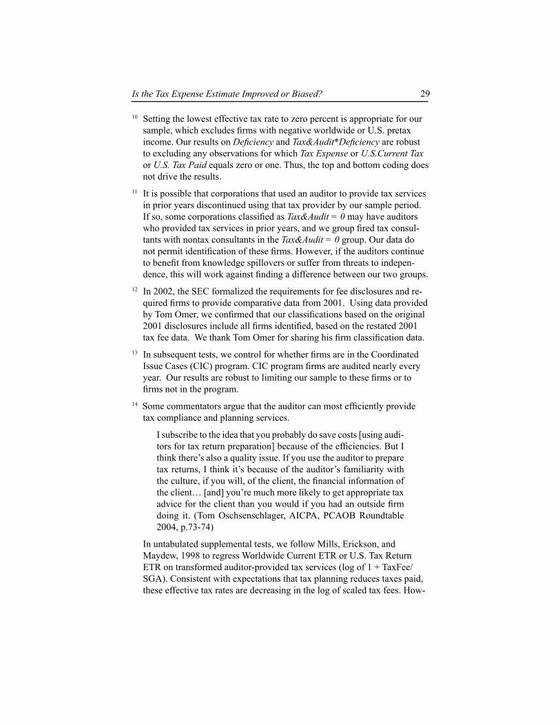
10 Setting the lowest effective tax rate to zero percent is appropriate for our sample, which excludes firms with negative worldwide or U.S. pretax income. Our results on Deficiency and Tax&Audit*Deficiency are robust to excluding any observations for which Tax Expense or U.S.Current Tax or U.S. Tax Paid equals zero or one. Thus, the top and bottom coding does not drive the results.
11 It is possible that corporations that used an auditor to provide tax services in prior years discontinued using that tax provider by our sample period. If so, some corporations classified as Tax&Audit = 0 may have auditors who provided tax services in prior years, and we group fired tax consul-tants with nontax consultants in the Tax&Audit = 0 group. Our data do not permit identification of these firms. However, if the auditors continue to benefit from knowledge spillovers or suffer from threats to indepen-dence, this will work against finding a difference between our two groups.
12 In 2002, the SEC formalized the requirements for fee disclosures and re-quired firms to provide comparative data from 2001. Using data provided by Tom Omer, we confirmed that our classifications based on the original 2001 disclosures include all firms identified, based on the restated 2001 tax fee data. We thank Tom Omer for sharing his firm classification data.
13 In subsequent tests, we control for whether firms are in the Coordinated Issue Cases (CIC) program. CIC program firms are audited nearly every year. Our results are robust to limiting our sample to these firms or to firms not in the program.
14 Some commentators argue that the auditor can most efficiently provide tax compliance and planning services.
I subscribe to the idea that you probably do save costs [using audi-tors for tax return preparation] because of the efficiencies. But I think there’s also a quality issue. If you use the auditor to prepare tax returns, I think it’s because of the auditor’s familiarity with the culture, if you will, of the client, the financial information of the client… [and] you’re much more likely to get appropriate tax advice for the client than you would if you had an outside firm doing it. (Tom Oschsenschlager, AICPA, PCAOB Roundtable 2004, p.73-74)
In untabulated supplemental tests, we follow Mills, Erickson, and Maydew, 1998 to regress Worldwide Current ETR or U.S. Tax Return ETR on transformed auditor-provided tax services (log of 1 + TaxFee/SGA). Consistent with expectations that tax planning reduces taxes paid, these effective tax rates are decreasing in the log of scaled tax fees. How-

Gleason and Mills30
ever, this test cannot determine whether auditor-provided tax services are more effective than other types of tax planning because the audit fee data do not report tax services. We consider annual regressions to learn whether the negative relation between fees and tax savings degrades over the sample period, consistent with Omer et al., 2005. For the full sample, Worldwide Tax Expense is negatively related to fees only in 2000, but not in any other year. Tax return ETR is negatively related to fees in 2001 but not in 2000 or 2002 (the last year of tax return data available). Although we are reluctant to make too much of these fragile results, we do not dispute Omer et al.’s result that the negative relation between auditor-pro-vided tax services and tax payments declines over the period. Additional details are available from the authors on request.
15 The U.S. Current Tax regression is qualitatively similar to Table 4 in that the net effect of the main and the interaction terms for Deficiency is zero, although the negative interaction is not significant by itself. The Cushion regression is not robust to this specification. However, a robustness test associating Worldwide Tax Expense with Deficiency is robust to using the tax fee ratio in place of our dummy variable
16 When we exclude other control variables from the regression, the coef-ficient on U.S. Tax Paid is 0.80 (std. error = 0.0429).
17 If the taxpayer prefers to file a claim for refund with the U.S. District Court of the U.S. Court of Claims, the corporation would prepay the tax prior to going to court. However, such a prepayment is unlikely to occur until the taxpayer has concluded the appeals process.
18 Slemrod and Blumenthal, 1993 document that compliance costs include both internal tax department costs (salaries and information technology costs) and external consulting services. The external services include both accounting and attorney fees. For the large corporations we study, we expect that corporations obtain tax planning services from multiple sources, including inhouse expertise. Thus, the choice to use auditor-pro-vided tax services does not represent a decision to conduct tax planning. We include taxes from the U.S. tax return in our main tests to control for differences in tax planning.
19 Using compliance cost survey data from Slemrod and Blumenthal, 1996, we confirm that the proportion of tax planning services of tax services purchased from accountants is negatively related to Combative and posi-tively related to OptionPct.
20 In an untabulated test, we find that auditor tenure (the number of years for which the corporation has used the same auditor) is no different among

Is the Tax Expense Estimate Improved or Biased? 31
the Tax&Audit groups. Thus, firms do not appear to have selected their tax providers based on specific tax positions taken. Further, we do not observe an ex ante explanation (Tenure) for maintaining a tax relationship with the auditor.
21 Evidence in Dhaliwal, Gleason, and Mills, 2004 shows that, on average, firms increase earnings by 1.6 cents by managing tax expense.
22 Relatedly, Blouin and Tuna, 2006 investigate whether cushion permits earnings smoothing. They find that net earnings are smoother than pretax earnings net of cash taxes paid plus stock option benefit.
23 The only penalty data we have available relates to the penalty for failure to file a return, which applies to less than one-third of 1 percent of the returns, using a sample of 8,674 closed return-years from 1994-2003. Our anecdotal understanding is that penalties for reasons other than nonfiling or nonpayment are rarely assessed and collected from large companies.
24 We base this estimate on a broader sample of 1,406 returns from 1994 from our match of Compustat, tax return, and IRS examination data for which the return is closed. It is possible that some exams for the 1994 return were still open after 2003, the last year for which data were available.
ReferencesAntle, Rick; Gordon, Elizabeth; Narayanamoorthy, Ganapathi; and Zhui,
Ling (2002), The Joint Determination of Audit Fees, Non-Audit Fees and Abnormal Accruals, working paper, Yale University.
Ashbaugh, Hollis; Lafond, Ryan; and Mayhew, Brian (2002), Do Nonaudit Services Compromise Auditor Independence?, The Accounting Review 78(3), pp. 611-639.
Beck, Paul; Frecka, Thomas; and Solomon, Ira (1988), A Model of the Market for MAS and Audit Services: Knowledge Spillovers and Auditor-Auditee Bonding, Journal of Accounting Literature, pp. 50-64.
Blouin, Jennifer and Tuna, Irem (2006), Tax Contingencies: Cushioning the blow on earnings from tax audits and policy changes, working paper, University of Pennsylvania.
Brown Larry D. and Caylor, Marcus L. (2005), A Temporal Analysis of Thresholds: Propensities and Valuation Consequences, The Accounting Review 80 (2), pp. 539-562.

Gleason and Mills32
Chung, Hyeesoo and Kallapur, Sanjay (2003). Client Importance, Nonaudit Services, and Abnormal Accruals, The Accounting Review 78(4), pp. 931-955.
Comprix, Jospeh; Mills, Lillian F.; and Schmidt, Andrew P. (2006), Earnings Management through Changes in Interim Expenses, Columbia University working paper.
Das, Somnath and Shroff, Pervin K. (2002), Fourth Quarter Reversals in Earnings Changes and Earnings Management, working paper, University of Minnesota.
Davidson, R. and MacKinnon, J.G. (1993), Estimation and Inference in Econometrics, Oxford University Press, New York.
DeAngelo, Linda E. (1981), Auditor Independence, ‘Low Balling’, and Dis-closure Regulation, Journal of Accounting and Economics 3, pp. 113-128.
Defond, Mark; Raghunandan, K.; and Subramanyam, K.R.. (2002), Do Nonaudit Service Fees Impair Auditor Independence? Evidence from Going Concern Audit Opinions, Journal of Accounting Research 40(4), pp. 1247-1243.
Dhaliwal, Dan; Gleason, Christi; and Mills, Lillian (2004), Using Income Tax Expense To Achieve Analysts’ Targets, Contemporary Accounting Research, Summer, Volume 21, Number 2, pp. 431-459.
Francis, Jere R.; Maydew, Edward L.; Sparks, H. Charles (1999), The Role of Big 6 Auditors in the Credible Reporting of Accruals, Auditing: A Journal of Practice and Theory, Volume 18, Number 2, pp. 17-34.
Frankel, Richard; Johnson, Marilyn; and Nelson, Karen (2002), The Relation Between Auditor’s Fees of Nonaudit Services and Earnings Management, The Accounting Review 77 (Supplement), pp. 71-105.
Gleason, Cristi and Mills, Lillian (2002), Materiality and Contingent Tax Liability Reporting, The Accounting Review, pp. 317-342.
Gleason, Cristi and Mills, Lillian (2006), Evidence of Differing Market Responses to Meeting or Beating Targets Through Tax Expense Decreas-es, working paper, University of Iowa.

Is the Tax Expense Estimate Improved or Biased? 33
Greene, William H. (2003), Econometric Analysis, Prentice-Hall, Inc., UpperSaddle River, New Jersey.
Grubert, Harry and Slemrod, Joel, The Effect of Taxes on Investment and Income Shifting to Puerto Rico, The Review of Economics and Statistics 80, Number 3, August 1998, pp. 365-373.
Gupta, Sanjay and Newberry, Kaye (1997), Determinants of the variability in corporate effective tax rates: Evidence from longitudinal data, Journal of Accounting and Public Policy, Volume 16, Number 1, pp. 1-34.
Hanlon, Michelle and Shevlin, Terry (2002), The Accounting Treatment of the Tax Benefits of Employee Stock Options: Implications for Financial Accounting and Tax Research, Accounting Horizons 16, Number 1, March, pp. 1-16.
Jacob, John and Jorgensen, Bjorn N. (2005), Earnings Management and Ac-counting Income Aggregation, working paper, University of Colorado at Boulder.
Kinney, William and Libby, Robert (2002), Discussion of The Relation Between Auditor’s Fees of Nonaudit Services and Earnings Management, The Accounting Review 77, pp. 107-114.
Kinney, William R., Jr.; Palmrose, Zoe-Vonna; and Scholz, Susan (2004), Auditor Independence, Non-Audit Services, and Restatements: Was the U.S. Government Right?, Journal of Accounting Research, Volume 42, Number 3, pp. 561-588.
Land, Judy and Lang, Mark H. (2002), Empirical Evidence on the Evolution of International Earnings, The Accounting Review 77, Supplement, pp. 115-134.
Lang, Mark H.; Ready, Jana S.; and Wilson, Wendy (2005), Earnings Man-agement and Cross Listing: Are Reconciled Earnings Comparable to US Earnings?, forthcoming, Journal of Accounting and Economics.
Leuz, Christian; Nanda, Dananjay; and Wysocki, Peter D. (2003), Earnings Management and Investor Protection: An International Comparison, Journal of Financial Economics, Volume 69, Number 3, pp. 505-527.

Gleason and Mills34
Larker, David and Richardson, Scott (2004), Fees Paid to Audit Firms, Accrual Choices, and Corporate Governance, Journal of Accounting Research, Volume 42, Number 3, pp. 625-658
Maydew, Edward and Shackelford, Douglas (2006), The Changing Role of Auditors in Corporate Tax Planning, University of North Carolina work-ing paper, NBER Working Paper 11504, August 2005.
Mills, Lillian; Erickson, Merle; and Maydew, Ed (1998), Investments in Tax Planning, Journal of the American Taxation Association, Volume 20, Number 1, pp. 1-20.
Mills, Lillian and Newberry, Kaye (2004), Do Foreign Multinationals’ Tax Incentives Influence their U.S. Income Reporting and Debt Policy?, National Tax Journal, March.
Myers, James; Myers, Linda; and Skinner, Douglas (2005), Earnings Momentum and Earnings Management, working paper, University of Chicago.
Omer, Thomas; Bedard, Jean; and Falsetta, Diana (2005), Auditor-Provided Tax Services: The Effects of a Changing Regulatory Environment, work-ing paper, Texas A&M University.
Reynolds, J. and Francis, Jere (2001), Does Size Matter? The Influence of Large Clients on Office Level Auditor Reporting Decisions, Journal of Accounting and Economics, Volume 30, pp. 375-400.
Rogers, W. (1993), Regression Standard Errors in Clustered Samples, In Stata Technical Bulletin Reprints, 1993, Volume 13, Stata Press, College Station, Texas.
Securities and Exchange Commission (SEC) (2000), Final Rule: Revision of the Commission’s Auditor Independence Requirements, Government Printing Office, Washington, DC.
Securities and Exchange Commission (SEC) (2003), Final Rule: Strength-ening the Commission’s Requirements Regarding Auditor Independence, Government Printing Office, Washington, DC.
Simunic, Dan. (1984), Auditing, Consulting, and Auditor Independence, Journal of Accounting Research, Volume 22, pp. 679-702.

Is the Tax Expense Estimate Improved or Biased? 35
Slemrod, J. and Blumenthal, M. (1993), The compliance costs of big busi-ness, The Tax Foundation, Washington, DC.
StataCorp (1999), Stata Statistical Software, Release 6.0., User’s Guide, Stata Press, College Station, TX, [U] 23.11, pp. 256-260.
White, H. (1980), A heteroskedasticity-consistent covariance matrix estima-tor and a direct test for heteroskedasticity, Econometrica, Volume 48, Number 4, pp. 817-838.
Zimmerman, J. (1983), Taxes and Firm Size, Journal of Accounting and Economics, August, pp. 119-149.
Appendix: Variable Definitions (# refers to Compustat item number)Tax Expense Measures:Worldwide Tax Expense = tax expense (#16) divided by pretax income
(#170). Cushion = U.S. current tax expense (#63, or current tax expense (#16 – #50,
or #16 if #50 missing) if #63 is missing) minus unscaled Option Tax Benefit minus Tax After Credits from the U.S. Tax Return, divided by pretax income (#170).
Worldwide Current Tax = current tax expense (#16 – #50, or #16 if #50 miss-ing) divided by pretax income (#170).
U.S. Current Tax= U.S. current tax expense (#63, or current tax expense (#16 – #50, or #16 if #50 missing) if #63 is missing) divided by pretax income (#170).
U.S. Tax Paid = Tax After Credits from the U.S. tax return, divided by pretax income (#170).
Option Tax Benefit = the tax benefit from stock options disclosed in the statement of cash flows or the reconciliation of stockholders equity. Where the amount is not disclosed, we compute Option Tax Ben-efit to equal 35 percent times the number of share exercised times the difference between the average stock price for the year less the average exercise price. If the latter computation is negative, we use the maximum stock price for the year in place of the average stock price. Finally, we set the benefit to zero where it is missing or nega-tive. Option Tax Benefit is scaled by pretax income (#170).
State Current Tax = State current tax expense (#173 if nonmissing, otherwise zero) divided by pretax income (#170).
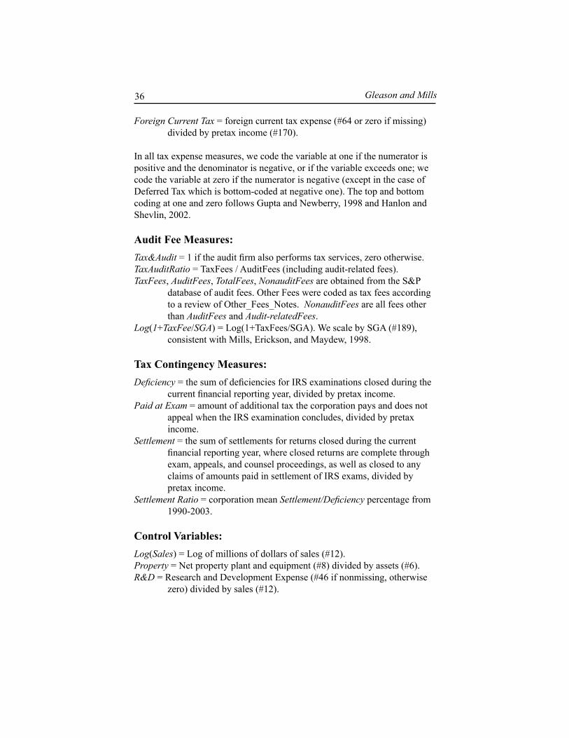
Gleason and Mills36
Foreign Current Tax = foreign current tax expense (#64 or zero if missing) divided by pretax income (#170).
In all tax expense measures, we code the variable at one if the numerator is positive and the denominator is negative, or if the variable exceeds one; we code the variable at zero if the numerator is negative (except in the case of Deferred Tax which is bottom-coded at negative one). The top and bottom coding at one and zero follows Gupta and Newberry, 1998 and Hanlon and Shevlin, 2002.
Audit Fee Measures:Tax&Audit = 1 if the audit firm also performs tax services, zero otherwise. TaxAuditRatio = TaxFees / AuditFees (including audit-related fees).TaxFees, AuditFees, TotalFees, NonauditFees are obtained from the S&P
database of audit fees. Other Fees were coded as tax fees according to a review of Other_Fees_Notes. NonauditFees are all fees other than AuditFees and Audit-relatedFees.
Log(1+TaxFee/SGA) = Log(1+TaxFees/SGA). We scale by SGA (#189), consistent with Mills, Erickson, and Maydew, 1998.
Tax Contingency Measures:Deficiency = the sum of deficiencies for IRS examinations closed during the
current financial reporting year, divided by pretax income. Paid at Exam = amount of additional tax the corporation pays and does not
appeal when the IRS examination concludes, divided by pretax income.
Settlement = the sum of settlements for returns closed during the current financial reporting year, where closed returns are complete through exam, appeals, and counsel proceedings, as well as closed to any claims of amounts paid in settlement of IRS exams, divided by pretax income.
Settlement Ratio = corporation mean Settlement/Deficiency percentage from 1990-2003.
Control Variables:Log(Sales) = Log of millions of dollars of sales (#12). Property = Net property plant and equipment (#8) divided by assets (#6). R&D = Research and Development Expense (#46 if nonmissing, otherwise
zero) divided by sales (#12).

Is the Tax Expense Estimate Improved or Biased? 37
1994 1995 1996 1997 1998 1999 2000
A) Corporation B) Corporation files C) IRS begins exam D) IRS concludes E) Corporation conducts tax 1994 return on 6/1/97. exam on 10/20/98. settles with IRS planning and on 9/15/05. Firm concedes/pays for some or all
records transactions. some, appeals rest. of appeal on 2/1/2000.
Foreign = absolute value of (foreign pretax income, #273 if nonmissing, zero otherwise, divided by pretax income, #170).
Except for the tax rate variables which are top and bottom coded, we win-sorize the explanatory and control variables at 1 percent and 99 percent.
AppendixTimeline and Illustration of Variable Definitions
The Timeline above illustrates the IRS examination process for a single tax return. We exclude prior and subsequent tax return years from our timeline, but those examinations would overlap with the tax period described.
We begin our illustration with the Calendar Year 1994 tax return. At year-end, managers accrue current and deferred tax liabilities, taking into account any amounts of tax benefit the company will probably lose due to IRS challenge. Independent auditors review managers’ recorded estimates of the tax accrual as part of the audit of the financial statements. Following the auditor’s attestation, the corporation releases earnings and files SEC Form 10K. Most corporations file their tax returns on the extended due date, 8 1/2 months after yearend. Our corporation would file its 1994 Form 1120 on September 15, 1995. We label the total tax after credits on the return as U.S. Tax Paid.
The IRS generally has 3 years from the date of filing to examine the tax return but will ask the taxpayer to extend the statute of limitations to allow time to complete the examination. In our example, the IRS begins the examination in 1997. The IRS designates certain taxpayers as being in the Coordinated Issue Cases program, also known as the “large-case audit” program. These corpora-tions expect to be audited nearly every year, so that there is little information in the knowledge that the IRS is beginning an examination. Other firms are audited with less frequency.
In our example, the IRS completes its examination in 1998. The IRS could require several years to conduct the examination, particularly if it audits several tax years as a group (called a “cycle”). In our sample, IRS exams for 1994 returns conclude an average of 4.6 years after the year for which the return was filed, with a range from 1 year to 9 years to conclusion.24 The IRS records

Gleason and Mills38
an ExamDate when the examination is complete, and the taxpayer responds to any additional tax (Deficiency) that the IRS proposes to the taxpayer. This date is usually within 90 days of the Notice of Deficiency and represents the date the taxpayer agrees to or appeals the adjustment, or the date of statutory assessment if the taxpayer fails to respond to the Notice.
The corporation pays none, some, or all of the Deficiency. We label the amount paid as Paid at Exam. Whatever the corporation does not pay it disputes by filing an appeal. The IRS has divisions for Examination, Appeals, and Counsel. Counsel handles court cases for the IRS and has final authority to concede and negotiate a settlement out of court.
The IRS considers a return to be closed when no claims by the IRS or by the taxpayer remain outstanding. In our example, the corporation settles the dispute in 2000 and pays any final amount negotiated with the IRS or decided by the court. For purposes of measuring a settlement date for our tests, we use the latest date that the IRS records a posting in Appeals or Counsel for any returns that the IRS designates as “closed.” We label the sum of all amounts paid during the examination, appeals, or counsel processes as Settlement.
A First Look at the 2004 Schedule M-3 Reporting by Large
Corporations* Charles Boynton and Ellen Legel, Internal Revenue Service, and
Portia DeFilippes, Office of Tax Analysis
For most publicly traded and many privately held corporations with assets of $10 million or more, the new Schedule M-3 book-tax reconciliation replaced the 4-decade-old Schedule M-1 effective December 2004. First,
we review events leading to the replacement of Schedule M-1 with Schedule M-3. We then present 2004 Schedule M-3 data and other tax data for corpora-tions filing the 2004 Form 1120, U.S. Corporate Income Tax Return, for the period December 2004 through June 2005 and reporting total assets of $10 million or more on the Form 1120 Schedule L balance sheet.1
Dissatisfaction with Schedule M-1A Treasury report in 1999 and Treasury testimony in 2000 by Assistant Secretary (Tax Policy) Jonathan Talisman noted the growing book-tax gap from 1991 to 1997 between pretax book income on Schedule M-1 and tax net income on page 1 of Form 1120. Both the report and the testimony viewed the 1990s book-tax gap as a possible indicator of corporate tax shelter activity, but also noted the difficulty in interpreting Schedule M-1 book-tax difference data.2 Mills-Plesko (2003) proposed a redesign of Schedule M-1 to increase the transparency of the corporate tax return book-tax reconciliation and to improve data interpret-ability.3 The Mills-Plesko (2003) Schedule M-1 recommendations are largely reflected in Schedule M-3, particularly in Part I.4
Schedule M-3Exhibit I presents the 2004 Form 1120. Part I reconciles worldwide consolidated financial statement income with income per income statement of includible cor-porations (members of the tax return consolidation group listed on Form 851). Parts II and III reconcile income per income statement of includible corpora-tions (“book”) with tax net income on Form 1120, page 1, line 28. Differences between book and tax are characterized as temporary or permanent.
The goal of the Schedule M-3 is greater transparency and uniform organi-zation in book-tax data at the time of return filing so that the data may be used

Boynton, Legel, and DeFilippes40
to determine what returns will and will not be audited, and to determine what issues will and will not be examined on the returns selected for audit.
Part I of Schedule M-3 is important. It defines the starting point for the book-tax reconciliation for the first time in corporate tax history. On Schedule M-1, we know where the reconciliation ends (tax net income), but not where it begins (book). Schedule M-3 Part I line 11 is what Schedule M-1 line 1 should have been. Schedule M-3 Part I is one of the revisions proposed by Mills-Plesko (2003).
Parts II and III reconcile financial net income of includible corporations to taxable income reported on Form 1120, page 1, line 28. Part II generally reconciles items of income, gain, and loss. Part III deals with expense and deduction items.
Parts II and III contain four columns to identify and differentiate the book and tax aspects of each line item. Column (a) represents financial statement income or expense amounts maintained in the corporation’s books and records, using the income statement source determined in Part I. Column (d) represents amounts as reflected in the tax return. For each line item, the difference between the amount shown in column (a) and the amount shown in column (d) is shown either as a temporary difference in column (b) or as a permanent difference in column (c). The clear statement of both the book and tax amounts, as well as the reconciling differences, aids the IRS in setting materiality thresholds for the reconciling differences shown.
The reporting of column (a) book income amounts and column (d) tax income amounts is optional for the first year a corporation is required to file Schedule M-3. In 2004, approximately 38 percent of the corporations with useable Schedule M-3 data (reporting approximately 56 percent of the aggregate tax after credits of such corporations) did not complete columns (a) and (d).
The detail required by Parts II and III is particularly enhanced by the differentiation of temporary and permanent differences. Temporary (timing) differences occur because tax laws require the recognition of some items of income and expense in different periods than are required for book purposes. Temporary differences originate in one period and reverse or terminate in one or more subsequent periods. Temporary differences between book and tax are questions of “when” not “if.” There are four basic categories of temporary differences:
1. Income recognized in financial statements before it is taxable;
2. Income reported as taxable before it is recognized in financial statements;
3. Expenses recognized in financial statements before they are deducted on the tax return; and,
4. Expenses deductible on the tax return before they are recognized on financial statements.

2004 Schedule M-3 Reporting by Large Corporations 41
By their very nature, such items involve issues regarding the correct year for the item’s inclusion in income or deduction as an expense. From a tax administration standpoint, they concern the time value of money. Over the lifetime of an entity, cycle of a specific transaction, or depreciable life of an asset, temporary differences between book and tax net to zero. Purely tem-porary differences are generally low risk for tax administration, and important in terms of the magnitude of the difference and the time before the temporary difference turns, due to the time value of money.
In contrast to temporary differences, permanent differences are adjust-ments that arise as a result of fundamental permanent differences in financial and tax accounting rules. These differences result from transactions that will not reverse in subsequent periods. In financial statement reporting under GAAP, permanent differences are not considered in the FAS Number 109 computation of deferred tax assets and liabilities, but do have a direct impact on the effective tax rate. Therefore, permanent differences have the potential to substantially influence reported earnings per share computations, and, in the case of public companies, stock prices. Accordingly, permanent differences of a comparable size generally have a greater audit risk than temporary differences.
Schedule M-3’s introduction of detailed reporting requirements for permanent and timing differences is another significant improvement over Schedule M-1, as well as an important enhancement to overall transparency. When examining Schedule M-1, the character of a particular book-tax differ-ence usually was not determinable without further investigation. Often, this required contacting the taxpayer, resulting in some degree of burden to both taxpayers and the IRS. In addition, the reporting of the book and tax amounts allows the IRS to consider the relative magnitude of the differences before contacting the taxpayer.
Source of 2004 Tax Return DataA statistical sample of tax return data is electronically-encoded annually by the Statistics of Income Division (SOI), Internal Revenue Service, for the use of the Office of Tax Analysis (OTA), U.S. Department of the Treasury, and the Joint Committee on Taxation (JCT), U.S. Congress. These data include Schedule M-1 data and beginning with 2004 include Schedule M-3 data. The annual SOI corporate file is issued to OTA and JCT in three versions in the second calendar year following the July-June tax year (in calendar 2006 for Tax Year 2004, that is, for corporate tax years ending July 2004 to June 2005). The Advance file is prepared by May 1, the Preliminary file prepared by September 1, and the Final file prepared by December 1. The Advance file contains a limited num-ber of “placeholder” records and uses tentative weights. The Preliminary file has far fewer placeholders and uses revised weights. The Final file has no

Boynton, Legel, and DeFilippes42
placeholders and uses final weights. Advance file placeholder records are data from the prior tax year for a few complex returns still undergoing SOI editing and for a larger number of late returns not yet received as of the issuance of the Advance file.5 Preliminary file placeholder records are for late returns not received as of the issuance of the Preliminary file. Placeholder records are eliminated for the Final file. The final weights compensate for missing returns not received as of the Final file. Researchers using SOI data may report only aggregate tax data for a minimum of three taxpayers to protect taxpayer confi-dentiality. For statistical reasons, SOI prefers that reported aggregate data are reported for 10 or more taxpayers whenever possible.
SOI annually summarizes selected tax return data from the Final corporate file in Publication 16, Corporate Income Tax Returns. Corporate tax data in the 2004 Final file prepared by December 2006 will be summarized in the 2004 SOI Publication 16 published in 2007. Our tax return table values may not add and may differ from official 2004 SOI Publication 16 values (when published in 2007) both due to rounding and because we used data from the 2004 SOI Advance corporate file made available to us 7 months before the issuance of the 2004 SOI Final corporate file.6
Tax Net Income and Intercompany Dividends (ICD)Form 1120, Schedule M-3, Part II, line 30, column (d) must equal Form 1120, page 1, line 28 when prepared by the corporate taxpayer. Some taxpayers improperly include U.S. intercompany dividends (ICD) in tax net income on Form 1120 page 1 line 28, the reconciliation target for Schedule M-3.7 The tax-payer then removes the same ICD amount as a 100 percent dividends-received deduction on line 29b so that it does not increase final income subject to tax on line 30. If the taxpayer includes ICD on Form 1120, page 1, line 28, he or she must also include it on Schedule M-3, Part II, line 30, column (d).
In general, ICD should be eliminated in determining tax net income. SOI removes all ICD amounts that it identifies in tax net income in the SOI corporate file.8 If the taxpayer includes ICD in tax net income on Schedule M-3, Part II, line 30, column (d) and on Form 1120, page 1, line 28, the tax net income reported on Schedule M-3, line 30, column (d) will differ (be larger than) tax net income on Form 1120, page 1, line 28 in the SOI corporate file by the amount of the ICD removed by SOI from line 28.9
We estimate the ICD adjustment as the (unedited) Schedule M-3, Part II, line 30 column (d) amount minus the (edited) Form 1120, page 1, line 28 (if it is a positive difference) for corporations filing a consolidated return.

2004 Schedule M-3 Reporting by Large Corporations 43
Overview of Tables 1-11We present our analysis of the 2004 Schedule M-3 data from the SOI Advance corporate file in two types of tables. Tables 1 through 6 are distributional tables. Each focuses on a population characteristic and the distributional impact of that population characteristic on aggregate amounts for selected Form 1120 tax return variables and Schedule M-3 variables. Tables 1 through 6 each present an overall analysis of the population characteristic at the top of the table and then show the effect of asset size (four or six asset classes: over $25 billion, $2.5 billion to $25 billion, $250 million to $2.5 billion, $50 million to $250 million, $25 million to $50 million, and $10 million to $25 million). In Table 1, the three smaller asset classes are combined into a single $10 million to $250 million class because of the small number of placeholder returns (seven) in that combined class.10
Tables 7 through 11 are each an aggregate Schedule M-3, Table 7 for the total reconciled population, Tables 8 and 9 for two financial statement type populations identified in Table 4, and Tables 10 and 11 for two populations based on the reporting or nonreporting of columns A and D data identified in Table 3.
Pretax Benchmark for Schedule M-3 Differences and Sign ConventionsWe calculate all book-tax difference as pretax differences, that is, as the differ-ence between the pretax book (measured before Federal income tax expense), and the tax amounts (also pretax) reported on Schedule M-3. We do this so that we are always comparing pretax amounts consistent with the book-tax literature since Talisman (2000). To do this for total book tax differences reported on Part II, line 30 or Part III, line 36, we must back out Federal income tax expense from the columns (b) and (c) reconciliation differences reported by taxpayers on Part II, line 30 and Part III, line 36.
The prior literature defines the sign of a pretax book tax difference as positive if the book amount is higher than the tax amount. Schedule M-3 effectively reverses this convention by the nature of its reconciliation rules. A negative total difference in columns (b) and (c) of Parts II and III means that the book amount is higher.
Data Presented in Tables 1-6In Tables 1 through 6, we present selected Form 1120 tax return variables and Schedule M-3 variables. The tax net income in the third dollar column of Panel 1 of these tables is from Form 1120, page 1, line 28 and is after SOI editing to

Boynton, Legel, and DeFilippes44
remove ICD. In the fourth dollar column is our estimated ICD amount. The sum of those two columns is equal (except for taxpayer errors corrected by SOI) to the tax income amount for Schedule M-3, Part II, line 30, column (d) (shown in Panel 2 of Table 3 to 6 in the fourth dollar column). The fifth dollar column in Panel 1 of Tables 1 to 6 is worldwide financial statement income from Part I, line 4. The next to last dollar column in Panel 1 of Tables 1 to 6 is book income from Part II, line 30, column (a). The last dollar column in Panel 1 of Tables 1 to 6 is Federal income tax expense calculated from Part III, lines 1 and 2. The sum of Federal income tax expense and book income is pretax book income shown in the first dollar column of Panel 2 of Tables 3 to 6. The difference between pretax book income and M-3 tax income is shown as a temporary and a permanent pretax difference in Panel 2 of Tables 3 to 6. In addition, the total pretax difference is shown as well as the positive and negative components of the temporary and permanent pretax differences. Total pretax book-tax difference under the Talisman (2000) approach is pretax book minus tax net income after removal of ICD by SOI. In our data, the Talisman (2000) pretax book-tax difference is the negative of the sum of pretax temporary and permanent differences plus the ICD amount.
Data Availability for the 2004 Schedule M-3 Population (Tables 1 and 2)Table 1 identifies the population of tax returns on the 2004 SOI Advance corporate file potentially subject to the requirement to include the 2004 Form 1120 Schedule M-3. The first requirement is that the corporation files a Form 1120 and reports assets of $10 million or more on Form 1120, Schedule L.11 The 2004 SOI Advance file contains 33,353 records statistically representing 42,129 tax returns for corporations filing Form 1120 with total assets of $10 million or more.12 These 42,129 tax returns include 100 tax returns that are placeholder returns. A placeholder return is 2003 data for a record for which 2004 editing is not complete at the time the Advance file was issued.13 The 2004 Advance file includes 6,742 nonplaceholder returns for tax years ending November 2004 or earlier and 35,286 nonplaceholder tax returns for tax years ending December 2004 or later.
For our 2004 Schedule M-3 study, placeholder returns on the 2004 SOI Advance corporate file represent potential missing Schedule M-3 data if the tax year ends in December 2004 or later for a corporation with $10 million or more in assets. We estimate the possible importance to our study of placeholder returns and other returns that we eliminate for lack of reconciliation as missing data by determining the tax after credits associated with those returns.

2004 Schedule M-3 Reporting by Large Corporations 45
The 42,129 tax returns with which Table 1 begins (corporations on the 2004 Advance file filing Form 1120 with assets of $10 million or more) have an aggregate tax after credits of $186,297 million. The 35,286 nonplaceholder tax returns for tax years ending December 2004 or later on the 2004 Advance file represent approximately 86 percent of the tax after credits ($160,647 million). The 6,742 nonplaceholder tax returns for tax years ending November 2004 or earlier represent approximately 9 percent of the tax after credits ($16,178 million). The 100 placeholder tax returns on the Advance file represent ap-proximately 5 percent of the tax after credits ($9,473 million).
As we show in Table 2, if we assume all placeholders are in fact subject to Schedule M-3 (tax years ending December 2004 or later), we have nonplace-holder tax return data for 35,286 tax returns representing approximately 94 percent of the aggregate tax after credits for the 35,386 tax returns (35,286 plus 100 placeholders) on the 2004 SOI Advance file assumed potentially subject to the 2004 Schedule M-3 ($160,647 million compared to $160,647 million plus $9,473 million or $170,120).
Table 2 starts with the 35,286 nonplaceholder tax returns for tax years ending December 2004 or later and the 100 placeholder returns on the 2004 SOI Advance corporate file identified in Table 1 and identifies the population of 30,430 tax returns for which we have reconcilable Schedule M-3 data. We eliminate 2,418 returns for a lack of any Schedule M-3 reconciliation data.14
We eliminate 2,310 returns that present Schedule M-3 data but either (1) Part II, line 30 column (a) does not reconcile with Part I, line 11, or (2) Part II, line 30 columns (a), (b), and (c) do not reconcile with column (d).15 Finally, we eliminate 128 returns because Part II, line 28 and Part III, line 36 do not rec-oncile.16 The approximately 41 percent of corporations with assets below $25 million account for a large proportion of the Schedule M-3 data with problems. Approximately 7 percent of the returns potentially subject to the 2004 Schedule M-3 report no Schedule M-3 data (2,418 out of 35,386). Approximately 66 percent of the nonreporters (1,601 out of 2,418) have assets below $25 million. Approximately 7 percent of the returns potentially subject to the 2004 Schedule M-3 report Part II, line 30 data that do not reconcile (2,310 out of 35,386). Approximately 46 percent of this group (1,058 out of 2,310) have assets be-low $25 million. Approximately 37 percent of the returns with Part II, line 27 reconciliation problems (47 out of 128) have assets below $25 million.
The 30,430 tax returns that we retain from Table 2 (with Schedule M-3 data for which both Part II, line 30 and line 28 pass our reconciliation tests) have an aggregate tax after credits of $151,405 million. The 2,418 returns eliminated for no M-3 data have an aggregate tax after credits of $917 million. The 2,310 returns eliminated for Part II, line 30 problems have an aggregate tax after credits of $7,918 million. The 128 returns eliminated for Part II line 28 problems have an aggregate tax after credits of $407 million.

Boynton, Legel, and DeFilippes46
Summary: Assuming all placeholders are in fact subject to Schedule M-3 (tax years ending December 2004 or later), we have 35,286 nonplaceholder and 100 placeholder returns for a total of 35,386 returns assumed subject to 2004 Schedule M-3. We have out of these 35,386 returns, nonplaceholder usable Schedule M-3 data for 30,430 tax returns (86 percent of 35,386) representing approximately 89 percent of the aggregate tax after credits for the 35,386 tax returns on the 2004 SOI Advance file assumed potentially subject to the 2004 Schedule M-3 ($151,405 million compared to $170,120).
Reporting of Part II Columns (a) and (d) in 2004 (Table 3)Tables 3 through 7 focus on the 30,430 tax returns in 2004 which have Schedule M-3 reconcilable data. Tables 3 through 6 address specific characteristics of the 30,430 returns. Table 7 presents aggregate Schedule M-3 data for the 30,430 returns. Tables 8 through 11 present aggregate M-3 data for subpopulations of the 30,430 returns. We determine if a corporation is a publicly-traded company based on its answer to Part I, line 3a.
Table 3 examines the reporting of book income and tax income amounts in Parts II and III columns (a) and (d). With the exception of Part II, line 30, a corporation may omit the Parts II and III columns (a) and (d) line-by-line book income and tax income amounts in the first year that Schedule M-3 is required. Of the 30,430 corporations with reconcilable Schedule M-3 data, 11,681 (38 percent) with 56 percent of tax after credits omitted this information including 1,837 of the 3,922 publicly-traded companies (47 percent). Another 15,169 (50 percent) with 37 percent of tax after credits provided reconcilable column (a) and (d) information for Parts II and III and include 1,803 public companies (46 percent). The remaining 3,581 (12 percent) with 6 percent of tax after credits provided the information, but one or more of the columns (a) and (d) in Parts II and III did not reconcile. This group includes 282 public companies (7 percent). Nonreporting of columns (a) and (d) amounts appears to increase as the asset size of the firm increases.
Financial Statement Type Reported for Part I (Table 4)Table 4 separates the 30,430 returns by financial statement class based on the answers to Schedule M-3, Part I, lines 1a, 1b, and 1c. The four classes are: SEC 10-K, audited but not SEC 10-K, unaudited, and books and records (no financial statements or no answer to Part I line 1). The 4,195 returns (14 percent of 30,430) of corporations that file a SEC 10-K financial statement account for 70 percent of the tax after credits of the 30,430 returns with 2004 Schedule

2004 Schedule M-3 Reporting by Large Corporations 47
M-3 reconcilable data, 91 percent of the ICD, 95 percent of the net aggregate temporary pretax book-tax difference, and 69 percent of the net aggregate permanent pretax book-tax difference.
Reporting of Financial Statement Restatements (Table 5)Table 5 focuses on Schedule M-3, Part I, lines 2b and 2c which asks questions about current-year restatement of financial statements and restatements within the 5 years prior to the current year. The total population for Table 5 is the 30,430 returns with reconcilable Schedule M-3 data. The 29,120 not reporting a restatement are 96 percent of the returns but report only 79 percent of the tax after credits and only include 3,347 of the 3,922 publicly traded companies, or 85 percent. The 5 percent of returns that report restatements report 21 percent of the tax after credits and include 15 percent of the public companies.
Reporting of Book-Tax Difference by Industry (Table 6)Table 6 separates the 30,430 returns into five industry groups: manufacturing, finance, information, utilities and transportation, and all other.17 The 30,430 returns report an aggregate book-tax difference of $131, 718 million, approxi-mately 38 percent permanent. The 6,351 returns in manufacturing report an aggregate net pretax book-tax difference of $98,810 million, approximately 75 percent of the total aggregate net pretax book-tax difference for the 30,430 returns. The difference is approximately 71 percent permanent. The 7,882 returns in finance report an aggregate net pretax book-tax difference of $12,267 million, approximately 9 percent of the total aggregate net pretax book-tax difference for the 30,430 returns. The difference is approximately 60 percent permanent. The 1,772 returns in information report an aggregate net pretax book-tax difference of positive $16,349 million, approximately 12 percent of the total aggregate net negative pretax book-tax difference for the 30,430 returns. The permanent difference component is positive $20,879 million.
Aggregate 2004 Schedule M-3 for U.S. Corporations (Table 7)Table 7 presents aggregate Schedule M-3 data for the 30,430 tax returns with reconcilable Schedule M-3 data. The data are present in three panels. Panel 1 provides population overview data in its first section, data for Schedule M-3,

Boynton, Legel, and DeFilippes48
Part I in its second section, and data reconciling Part I book with Part II tax income, and SOI tax net income in its third section.
The first data section of Panel 1 of Table 7 reports aggregate total assets (Form 1120, Schedule L), tax less credits, and tax net income (Form 1120, page 1, line 28) for the 30,430 returns, reconciles the tax net income to the tax income reported by the taxpayers on Part II, line 30, column (d), and tax exempt interest (Form 1120, Schedule K, item 9).18
The second data section of Panel 1 of Table 7 presents aggregate Schedule M-3, Part I data for the 30,430 returns. Part I, line 4 reports aggregate world-wide financial statement income of $568,010 million. Part I lines 5 through 10 adjusts that to $515,422 million as aggregate book income of includible corporations. Part I, line 4 aggregate worldwide income is 110 percent of line 11 aggregate book income. Part I, line 5 removes $204,469 million (40 percent of book) for foreign entities and $86,534 million (17 percent of book) for U.S. entities included in the financial statement consolidation but not in the tax consolidation. Part I, line 7 adds $3,785 million (1 percent of book) for U.S. corporations not included in the financial statement consolidation but included in the tax consolidation. Part I, line 8 adds $184,101 million (36 percent of book) as adjustments to eliminations because of lines 5 through 7, usually the recognition of dividend income and adjustment to minority interest income. The net effect of Part I, lines 5 through 8 is to remove $103,118 million (20 percent of book). Part I, line 9 adds adjustments of $6,136 million (1 percent of book) for the difference between financial statement year and tax return year. Part I, line 10 adds other adjustments of $33,723 million (7 percent of book). Part I, line 10 will generally be used by corporations with insurance subsidiaries to reflect adjustments required by the use of statutory accounting for subsidiary book income. Statutory accounting for subsidiaries differs from generally accepted accounting principles (GAAP) accounting for financial statements, in particular, in the inclusion of certain intercompany dividends. Finally, Part I, line 11 includes $11,915 million (2 percent of book) not reflected in Part I, lines 4 through 10 for corporations with only books and records.19
The third data section of Panel 1 of Table 7 reconciles aggregate Schedule M-3, Part I, line 11, book data with Part II pretax temporary and permanent book-tax differences and with SOI-reported tax net income for the 30,430 returns.
Panel 2 of Table 7 presents aggregate Schedule M-3, Part II data for the 30,430 returns. We present aggregate net taxpayer data for book income amount (column (a)), temporary difference (column (b)), permanent difference (column (c)), tax income amount (column (d)), total difference (sum of columns (b) and (c)), and the total aggregate positive and negative reported differences for columns (b) and (c) that determined the net differences. We note that the net aggregate pretax temporary and permanent book-tax difference amounts

2004 Schedule M-3 Reporting by Large Corporations 49
are the net differences between relatively large aggregate positive and nega-tive temporary and permanent amounts and that the net differences are often small in comparison. We also present the frequency with which any nonzero amount was reported on the line.
At the foot of Panel 2, we present the necessary correction of the Schedule M-3 reconciliation totals to a pretax basis (before Federal income tax expense). Mechanically, Schedule M-3 compares book income after tax with pretax tax income and includes Federal income tax expense as a book expense in Part III. For analysis, it is necessary to correct the Schedule M-3 data to a consistent pretax basis (before Federal income tax expense). This has been the approach since Talisman (2000). To do this, we back out Federal income tax expense from book income.
Part II, line 30 reports a temporary difference of $74,502 million and a permanent difference of $134,455 million for a net difference of $59,953 mil-lion. Column (a) book is $515,421 million, and column (d) tax is $575,375 million. Tax income in column (d) is show as $59,953 million greater than column (a) book income. After correction to a pretax basis, pretax book income is $707,092. The tax income of $575,375 million is in fact less than pretax book income by $131,717 million.
We know Federal income tax expense from Part III, lines 1 and 2 even without column (a) data. Since column (d) is zero by definition, column (a) must be the negative of the sums of columns (b) and (c).
Federal income tax expense is $191,670 million, of which $7,085 million are classified as temporary, and $184,585 million are classified as permanent. Pretax book income is the sum of Federal tax expense and book income. The adjustment amounts for columns (b) and (c) must be in total the negative of the column (a) adjustment amount so that the adjustment has no effect on column (d) just as the original Federal tax expense had no effect on column (d). We adjust column (b) by $7,085 million and column (c) by $184,585 million. The result is that column (b) becomes slightly more negative and the sign of column (c) changes and becomes negative. The adjusted pretax column (b) temporary difference is $81,587 million, and the adjusted pretax column (c) is $50,131 million. The adjusted total pretax difference is ($131,718) million, the differ-ence between pretax book income of $707,092 million and pretax tax income of $575,375 million. Our pretax total difference benchmark is $131,718 million. Pretax book for 2004 is $707,092 million and is higher than tax net income of $523,015 on Form 1120, page 1, line 28 by $184,077 million, $131,718 million measured by Schedule M-1 plus $52,698 of ICD, plus $339 million of taxpayer errors not identified here.
The pretax total difference of $131,718 million is $81,587 million temporary (62 percent) and $50,131 million permanent (38 percent).

Boynton, Legel, and DeFilippes50
We express all total line difference as a percentage of pretax book to de-termine which lines contribute the most to the total difference. For example, the total aggregate net pretax book-tax difference of ($131,717) million is (18.6) percent of pretax book. Part II, line 13 interest income contributes ($15,053) million, or (2.1) percentage points of the net (18.6) percent.20
Panel 3 of Table 7 presents aggregate Schedule M-3, Part III data for the 30,430 returns. In Part III, we have changed the sign of all data to agree with Part II. We show deductions in Part III as negative amounts. Schedule M-3, Part III shows deductions as positive amounts and changes sign for the totals carried over to Part II, line 28.21 The signs of the differences we show in Part III indicate the effect of that expense or deduction on the net difference between pretax book and tax income.
A few of the lines on Parts II and III account for most of the net negative difference of 18.6 percentage points of pretax book. Some lines contribute to the net negative difference of 18.6 percentage point of pretax book, and some lines offset that net negative difference. The largest net negative difference on a line with a specific description is not unexpected. Part III, line 31, depreciation, reports tax depreciation greater than book for a net effect of $112,778 million, contributing 15.9 percentage points to the total pretax difference of 18.6 percent of pretax book. The effect of depreciation is almost all temporary.
Part II, line 12 reportable transactions, reports book higher than tax by $44,837 million, contributing 6.3 percentage points to the total pretax difference of 18.6 percentage points of pretax book. The effect of reportable transactions is largely temporary, but, with a substantial permanent component, Part III, line 9, nonqualified stock options, reports tax deductions greater than book expense for a net effect of $40,430, contributing 5.7 percentage points of pretax book. The effect of stock options is almost all permanent. Part III, line 16, pension and profit-sharing, reports tax deductions greater than book expense for a net effect of $17,972 million, contributing 2.5 percentage points of total pretax difference. The effect of pensions is largely temporary.
In the other direction, Part III, line 28, other amortization or impairment writeoffs, reports book expense greater than tax for a net effect of $50,865 mil-lion, offsetting 7.2 percentage points of total pretax difference. The effect of amortization and impairments has both substantial temporary and permanent components. Part II, line 17, inventory valuation adjustment (cost of goods sold), reports book lower than tax by $45,611 million, offsetting 6.5 percentage points of the 18.6-percent pretax total. The effect of inventory adjustments is almost all temporary. Part II, line 18, Sale versus lease (for sellers and /or lessors), reports book lower than tax by $29,324 million, offsetting 4.1 percent-age points of the 18.6-percent pretax total. The effect of sale versus lease is almost all temporary.

2004 Schedule M-3 Reporting by Large Corporations 51
Part II, line 9, U.S. partnerships, reports book lower than tax by $18,861 million, offsetting 2.7 percentage points of the total pretax difference.
Note that the differences on Part II, lines 23a and 23b for asset disposi-tion (book) and capital gain transactions (tax) are almost offsetting and reflect the structure of Schedule M-3 which separates the accounting on two separate book and tax lines.
Perhaps the most interesting line difference is that for Part II, line 26 other income (loss) items with difference with book higher than tax by $116,892 million contributing 16.5 percentage points of the 18.6-percent pretax total. The effect of this line has approximately equal temporary and permanent components.22
Aggregate 2004 Schedule M-3: SEC 10-K Financial Statements (Table 8)Table 8 presents aggregate Schedule M-3 data for the 4,195 returns out of the 30,430 tax returns with reconcilable Schedule M-3 data that have SEC 10-K financial statements. These returns report a pretax difference of $112,019 million, that is book higher than tax, 85 percent of the total difference for the 30,430. The temporary difference of $77,512 is 95 percent of the total tempo-rary difference for the 30,430. The permanent difference of $34,507 million is 69 percent of the total permanent difference for the 30,430.
Aggregate 2004 Schedule M-3: Audited Financial Statements (Table 9)Table 9 presents aggregate Schedule M-3 data for the 13,544 returns out of the 30,430 tax returns with reconcilable Schedule M-3 data that have audited finan-cial statements that are not SEC 10-K. These returns report a pretax difference of $34,250 million, that is book higher than tax, 26 percent of the total differ-ence for the 30,430. The temporary difference of $14,870 is 18 percent of the total temporary difference for the 30,430. The permanent difference of $19,380 million is 39 percent of the total permanent difference for the 30,430.
Aggregate 2004 Schedule M-3: Columns A and D Reconcile (Table 10)Table 10 presents aggregate Schedule M-3 data for the 15,169 returns out of the 30,430 tax returns with reconcilable Schedule M-3 data in Parts II and III columns (a) and (d). These returns report a pretax difference of $46,322 million, that is, book higher than tax, 35 percent of the total difference for the

Boynton, Legel, and DeFilippes52
30,430. The temporary difference of $3,807 is 5 percent of the total temporary difference for the 30,430. The permanent difference of $42,515 million is 85 percent of the total permanent difference for the 30,430.
Aggregate 2004 Schedule M-3: Columns A and D Blank (Table 11)Table 11 presents aggregate Schedule M-3 data for the 11,681 returns out of the 30,430 tax returns with reconcilable Schedule M-3 data and blank Parts II and III columns (a) and (d). These returns report a pretax difference of $73,083 million, that is book higher than tax, 55 percent of the total difference for the 30,430. The temporary difference of $68,006 is 83 percent of the total tempo-rary difference for the 30,430. The permanent difference of $5,077 million is 10 percent of the total permanent difference for the 30,430.
Review of Supporting Documentation for Selected Schedule M-3 linesOne of the authors23 reviewed in excess of 100,000 pages of 2004 Schedule M-3 documentation for more than 100 tax returns, each reporting a positive or negative amount of more than $10 million in absolute value on Part II, line 26, Other income (loss) items with differences; on Part III line 35, Other expense/deduction items with differences; or on Part I, lines 8 or 10, adjust-ments to eliminations and other adjustments. The following comments reflect that research.
Note: For 2004 and 2005, consolidated tax groups with a Form 1120 parent and insurance subsidiaries were permitted a shortcut to report all insur-ance subsidiary activity on Part II, line 26. That will change in 2006. Large temporary and permanent differences are reported on Part II, line 26 in 2004 as a result.
Negative and Positive Large Differences on Part II Line 26:Some companies report positive temporary and permanent differences on Part II, line 26 as intercompany dividends. Unless these are intercompany divi-dends of insurance subsidiaries subject to line 26 reporting in 2004 and 2005, they should be reported on Part II, line 7. In several cases, matching dividend amounts were not reported on Part I, line 10, suggesting that the dividends were not insurance-related.
Some companies use Part I, line 8 to reverse all or substantially all financial statement eliminations, and then use Part II, line 26 to remove income

2004 Schedule M-3 Reporting by Large Corporations 53
improperly included on Part I, line 11 as a result of the Part I, line 8 reversals. Part I, line 11 should be the amount of consolidated financial statement net income of includible corporations (the consolidated tax group listed on Form 851) after all appropriate eliminations.
Some companies report intercompany dividends on Part I, line 8 and report a negative permanent difference on Part II, line 26 as a reduction of those inter-company dividends subject to tax. If the dividends are foreign dividends that are intercompany dividends for financial accounting, but not for tax accounting, and if the negative adjustment reflects dividends representing previously taxed subpart F income, the adjustment should be reported on Part II, line 5.
Some companies use Part II, line 26 for “eliminations” of income without further explanation. This does not meet the standard of “separately stated and adequately described.”
Some companies report “Mark to market” on Part II, line 26. These amounts should have been reported on Part II, line 16.
Some companies use Part II, line 26 to report equity income or loss of subsidiaries. These amounts should be reported on Part II, lines 1 or 6.
Part II, line 26 was also used to report permanent positive difference totals in inventory valuation adjustments. These amounts should have been included on Part II, line 17.
Substantial temporary differences were reported as foreign exchange transaction gains/losses, as cancellation of debt income, and as royalty income. This is appropriate, but perhaps Schedule M-3 lines should be created for these items in the future.
Negative and Positive Large Differences on Part III Line 35:Large amounts of interest expense were reported on Part III, line 35. In 2005, interest expense is specified on a separate line in Part III.
Large amounts of writeoffs were reported on Part III, line 35. If these amounts represent writeoffs or change in reserve balances, each reserve should be separately stated and adequately described. If they represent writeoffs of goodwill, they should be reported on Part III, line 26, Amortization/impairment of goodwill. If they are writeoffs of assets, they should be reported on Part III, line 28, Other amortization or impairment writeoffs.
Negative and Positive Large Differences on Part I Lines 8 and 10:Part I, line 8 was generally used to adjust consolidation eliminations for en-tity income and loss removed or added on Part I, lines 5 through 7, which is appropriate. Note that 3,699 returns had entries on Part I, line 5, but only 1,736

Boynton, Legel, and DeFilippes54
had entries on Part I, line 8. Some companies removed foreign entity income or loss on Part I, line 5, but had no consolidation elimination adjustment on line 8. This may be appropriate if entities removed were 100-percent owned (no minority interest), carried on the cost basis (no equity income), and paid no dividends. The instructions for Part I, line 8 permit, but do not require, the reporting of zero net changes.
Part I, line 10 was generally used to report the addition of intercompany dividends, which is appropriate if the addition was required by statutory accounting for insurance subsidiaries of a Form 1120 parent. In 2004, the documentation is not always clear as to why intercompany dividends are added. In 2006, a new line 10a will separately report the addition of intercompany dividends required by statutory accounting.
Part I, line 10 was also used to report valuation adjustments, eliminations, addition of equity earnings, and the removal of income related to bankruptcy reorganization. It appears that these items should have been reported on Part I, lines 5 through 8, or within Parts II and III. In particular, the income reported on Part I, line 11 should be the share of the worldwide consolidated net income on Part I, line 4 that belongs to the includible corporations (the consolidated tax group listed on Form 851) after all appropriate consolidation eliminations. Part I, line 10 should not be used to reduce the book income on line 11 as a means of reducing the book-tax difference to be reconciled in Parts II and III.
Summary and ConclusionFor most publicly-traded and many privately-held corporations with assets of $10 million or more, the new Schedule M-3 book-tax reconciliation replaced the 4-decade-old Schedule M-1 effective December 2004. Part I reconciles worldwide consolidated financial statement income with income per income statement of includible corporations (members of the tax return consolida-tion group listed on Form 851). Parts II and III reconcile income per income statement of includible corporations (“book”) with tax net income on Form 1120, page 1, line 28. Differences between book and tax are characterized as temporary or permanent. Part I is considered extremely important. For the first time, the starting point for the book-tax reconciliation is specified.
We begin our analysis with 42,129 returns for corporation filing Form 1120 for 2004 with assets of $10 million or more. We eliminated 6,742 that have a November 2004 or earlier yearend. The remaining 35,386 include 100 placeholder returns that are potentially subject to the 2004 Schedule M-3. For the nonplaceholder 35,286, we determine that 30,430 have reconcilable Schedule M-3 data.
We estimate the possible importance to our study of placeholder records and other records that we eliminate for lack of reconciliation as missing data by

2004 Schedule M-3 Reporting by Large Corporations 55
determining the tax after credits associated with those records. Assuming all placeholders are in fact subject to Schedule M-3 (tax years ending December 2004 or later), our nonplaceholder usable Schedule M-3 data for 30,430 tax returns represent approximately 89 percent of the aggregate tax after credits for the 35,386 tax returns on the 2004 SOI Advance file assumed potentially subject to the 2004.
We discuss the need to convert Schedule M-3 data to pretax differences by backing out the effects of Federal tax expense. The adjustment to a com-mon pretax base for both book and tax is consistent with the literature since Talisman (2000). For the 30,430 returns with reconcilable Schedule M-3 data, pretax book is higher than tax income and in Schedule M-3 is reflected with a negative sign. For the 30,430 returns, Table 7 presents an aggregate net pretax total difference of $131,718 million of which $81,587 million are temporary (62 percent), and $50,131 million are permanent (38 percent).
Table 8 presents aggregate Schedule M-3 data for the 4,195 returns out of the 30,430 tax returns with reconcilable Schedule M-3 data that have SEC 10-K financial statements. These returns report an aggregate net pretax differ-ence of $112,019 million, that is book higher than tax, 85 percent of the total difference for the 30,430. The temporary difference of $77,512 is 95 percent of the total temporary difference for the 30,430. The permanent difference of $34,507 million is 69 percent of the total permanent difference for the 30,430. The share of tax after credits of these firms is 70 percent.
Perhaps the most interesting line difference in Table 7 for the 30,430 returns is that for Part II, line 26 other income (loss) items with difference.24 It is 89 percent of the total pretax difference with book higher than tax by $116,892 million with approximately equal temporary and permanent components (each 44 percent approximately of the total pretax difference.) The IRS needs to investigate the supporting documentation for Part II, line 26 and determine if some items included there should have new separate lines on Schedule M-3 in future years.
AcknowledgmentsCharles Boynton is a Program Manager and Senior Program Analyst with Strategy, Research, and Program Planning, Large and Mid-Size Business Divi-sion, Internal Revenue Service. From September 2000 through May 2006, he was a Surrey Senior Research Fellow, Office of Tax Analysis, U.S. Treasury. He has been a member of the joint Treasury-IRS Schedule M-3 team from its formation in June 2003.
Portia DeFilippes is a Financial Economist in the Economic Modeling and Computer Application Division, Office of Tax Analysis, U.S. Treasury. Begin-

Boynton, Legel, and DeFilippes56
ning in September 2000, she and Charles Boynton have explored comparisons of corporate financial statement and tax return data, book-tax differences, and tax return consolidation anomalies as part of their official research for OTA.
Ellen Legel is a Senior Staff Economist and Management Official with the Corporation Tax Branch of the Statistics of Income Division, Internal Revenue Service. She has been a Lead Analyst for the Corporation Tax Program and is the Senior Analyst for Schedule M-1, Schedule M-2, and Schedule M-3.
This paper was prepared for the 2006 IRS Research Conference and was presented on June 14, 2006, by Ellen Legel.
We thank the Statistics of Income (SOI) Division, Internal Revenue Service, for making data from the 2004 SOI Advance corporate file available to us for our research. We thank the following at SOI for assistance: Thomas Petska, Douglas Shearer, Janet McCubbin, Martha Harris, and, particularly, Ken Szeflinski. Also, thanks go to Mike Mandeville, Kathleen Walker, and Melissa Schottler for assistance with the Advance Data file. We thank Karen Gill, Publishing Division, and Barbara Bradley, Tax Forms and Publications Division, Internal Revenue Service, for providing Exhibit I, “2004 Form 1120, Schedule M-3.” We thank the participants in the May 12, 2006, OTA Brownbag Seminar, and the participants in the June 14, 2006, IRS Research Conference. We thank the following for comments at different stages of the development of the paper: Robert Adams, Geraldine Gerardi, Don Kiefer, John McClellan, Mike McDonald, Judith McNamara, John Miller, Lillian Mills, Susan Nelson, George Plesko, David Stanley, William Trautman, Bill Wilson, and Gregory Zielinski. Lastly, but not least, we thank Jonathan Mable for his PowerPoint presentation and both Jonathan Mable and Erin Sullivan for past and current assistance in our projects. All errors are ours alone.
Endnotes* First published in Tax Notes 112, No. 11 (September 11, 2006): 943-981.
Reprinted with permission. Prepared for the 2006 IRS Research Conference.
1 The current paper repeats certain material from Boynton, DeFilippes, and Legel (2005 and 2006) and from Boynton and Wilson (2006), used with permission. Our tax return table values may not add and may differ from official 2004 SOI Publication 16 values (when published in 2007) both due to rounding and because we used data from the 2004 SOI Advance corporate file made available to us 7 months before the issuance of the 2004 SOI Final corporate file. See the discussion of the Advanced file and Final file in Source of 2004 Tax Return Data. The SOI corporate data file for year t includes all tax years ending between July of Calendar

2004 Schedule M-3 Reporting by Large Corporations 57
Year t and June of Calendar Year t+1. Effective for all tax years ending on or after December 31, 2004, Schedule M-3 replaced Schedule M-1 for corporations filing Form 1120 and reporting total assets of $10 million or more on Form 1120, Schedule L. Effective December 2006, for corpora-tions with total assets of $10 million or more, Schedule M-3 will apply to Form 1120-S for S corporation, to Form 1120-C for cooperative associa-tions, and to Form 1120-L and Form-PC for life and property and casualty insurance companies. Effective December 2006, Schedule M-3 will also apply to Form 1065 for partnerships with total assets of $10 million or more and certain other partnerships. Schedule M-1 continues to apply to Form 1120-F for foreign corporations with effectively connected U.S. income, to Form 1120-RIC for regulated investment companies, to Form 1120-REIT for real estate investment trusts, and to all corporations with total assets of less than $10 million.
2 See U.S. Department of the Treasury (1999) and Talisman (2000). See also Mills (1998) cited by Treasury (1999, page 32, note 118): “Mills finds evidence that the IRS is more likely to assert deficiencies on firms with large book-tax disparities, indicating that such disparities are cor-related with aggressive tax planning.”
3 See Mills and Plesko (2003) for the proposed redesign of Schedule M-1. For discussions of problems in interpreting Schedule M-1 book-tax reconciliation data and problems with the related Schedule L book bal-ance sheet data, see Boynton, Dobbins, DeFilippes, and Cooper (2002), Mills, Newberry, and Trautman (2002), Boynton, DeFilippes, Lisowsky, and Mills (2004), Boynton, DeFilippes, and Legel (2005 and 2006), and Boynton and Wilson (2006). For discussions of the problems in reconcil-ing financial accounting income and tax income, see McGill and Outslay (2002), Hanlon (2003), McGill and Outslay (2004), Plesko (2004), and Hanlon and Shevlin (2005).
4 For a discussion of the development of Schedule M-3, see Boynton and Mills (2004).
5 Placeholder data are commonly the edited return data from the prior tax year, but may also be current- year data from the IRS Business Master File (limited return data tabulated by the IRS when the return is first received and processed) or, in the case of returns not yet received, current-year survey data collected by SOI directly from the taxpayer on a voluntary basis on a limited number of critical variables.
6 SOI Publication 16 tables have not presented Schedule M-1 data to date. Currently, it is not planned for SOI Publication 16 to present Schedule M-3 data. Prior to the publication of Boynton, DeFilippes, and Legel

Boynton, Legel, and DeFilippes58
(2005 and 2006), only Plesko (2002) (for 1996-1998) and Plesko- Shumofsky (2005) (for 1995-2001) presented Schedule M-1 data for the SOI Publication 16 population.
7 It is improper to include intercompany dividends in tax net income if a consolidated tax group does not contain an insurance company subsidiary. Schedule M-3 instructions recognize that consolidated tax groups contain-ing insurance company subsidiaries may be required for book account-ing (under statutory accounting rules for insurance companies), and tax accounting (under Federal income tax consolidation rules for insurance companies) to include certain intercompany dividends in book income and in tax income. See the 2004, 2005, and 2006 Form 1120 instructions for Schedule M-3, Part I, lines 10 and 11 and Part II, lines 7 and 26. In April 2006, Form 8916 was announced to supplement Schedule M-3 for certain mixed groups, including, in particular, tax consolidation groups with a Form 1120 parent and an insurance subsidiary. Form 8916 is used by mixed groups to reconcile tax net income on Schedule M-3 with tax-able income on the tax return.
8 On the SOI corporate file, SOI removes all intercompany dividends (ICD) that it identifies from Form 1120 data, including from page 1, line 28 whether or not the tax consolidation group contains an insurance compa-ny subsidiary. See the discussion of the history of ICD editing by SOI for 1990-2003 tax years in Boynton, DeFilippes, and Legel (2005 and 2006). Note that changes on the SOI corporate file do not change the amounts on the tax return and do not impact IRS audits (or lack of audits) for corpo-rate tax returns.
9 SOI also corrects certain taxpayer errors it finds on Form 1120, page 1. The observed difference between Schedule M-3, Part II, line 30, column (d) and Form 1120, page 1, line 28 on the SOI corporate file is the net effect of the SOI ICD adjustment and any other SOI error adjustments made on the SOI corporate file.
10 We may not report data for fewer than three taxpayers. See the discussion of placeholder returns in “Source of 2004 Tax Return Data” and “Data Availability for the 2004 Schedule M-3 Population (Tables 1 and 2).”
11 In fact, approximately 200 companies with assets less than $10 million voluntarily filed Schedule M-3. We do not analyze those data.
12 The SOI corporate file is a statistical sample. The record for a smaller tax return (usually measured by total assets) may be weighted to represent more than one tax return. Generally, tax returns for corporations with

2004 Schedule M-3 Reporting by Large Corporations 59
$50 million or more in assets have a weight of one, that is the record represents only itself. The record for a smaller tax return generally has a weight greater than one (for example five), that is, the record repre-sents several similar tax returns (for example, five tax returns). The total 2004 SOI Advance corporate file contains 112,928 records represent-ing 5,614,795 corporate tax returns reporting aggregate total assets of $59,983,334 million and aggregate tax after credits of $218,196 million. This total includes S corporations, regulated investment trusts, and real estate investment trusts. These do not normally pay corporate income tax. Excluding S, RIC and REIT, the 2004 SOI Advance file contains 63,739 records representing 2,045,501 corporate tax returns reporting ag-gregate total assets of $46,941,900 million and aggregate tax after credits of $217,705. The 33,353 records representing 42,129 corporation tax returns filed on Form 1120 each reporting assets of $10 million or more (2.1 percent of all corporate returns excluding S, RIC, and REIT) have aggregate total assets of $40,137,268 million (85.5 percent of all corpo-rate returns excluding S, RIC, and REIT) and aggregate tax after credits of $186,297 million (85.6 percent of all corporate returns excluding S, RIC, and REIT).
13 See “Source of 2004 Tax Return Data” for a fuller discussion of the sources of placeholder data.
14 We tested Part I, lines 4 through 11 and Part II, lines 26 through 30 for any nonzero amount. In particular, a book amount for the tax group should be reported on Part I, line 11, and a reconciliation between that amount and tax net income should be reported on Part II, line 30.
15 We also eliminate a return if Schedule M-3, Part II, line 30, column (a) or column (d) is exactly zero. We do not test the reconciliation between Part II, line 30, column (d) and Form 1120, page 1, line 28. Rather, if Part II, line 30, column d,is nonzero, we treat any positive difference with page 1, line 28 for a consolidated return as the measure of the ICD removed by SOI from page 1, line 28.
16 Part III is designed to report expenses and deductions as positive amounts. The column sums on Part III, line 36 are then carried over to Part II, line 28 with a sign change and added on Part II in determining Part II, line 30 column amounts. We test to see if Part II, line 28 columns (b) and (c ) are each the negative of those columns on Part III line 36, and if Part II, line 27 columns (b) and (c), and Part II, line 28, columns (b) and (c) each add to Part II, line 30 columns (b) and (c ). In addition to the 128 returns (103 records) that we eliminate with these tests, there were an additional 139 returns that initially failed. For 119 of the returns

Boynton, Legel, and DeFilippes60
that initially failed our tests, we determined that the taxpayer reported expenses and deductions on Part III as negative amounts and carried those amounts to Part II, line 28 without a sign change where these amounts could appropriately be added. For aggregation purposes in Tables 6-17, we changed the sign of amounts on Part III of these 119 returns so that expenses and deductions were reported as positive amounts. For 20 of the returns that initially failed our tests, we determined that the taxpayer reported expenses and deductions on Part III as positive amounts and carried those amounts to Part II, line 28 without a sign change where the taxpayer then subtracted the Part II, line 28 column amounts to determine Part II, line 30. For aggregation purposes in Tables 6-17, we changed the sign of amounts on Part II, line 28 so that those amounts could be added.
17 The major SOI industry sector codes are: manufacturing 31; finance (including real estate and holding companies) 52, 53, 55; information 51; utilities and transportation 22, 48.
18 Tax-exempt interest is a major component of the permanent difference reported on Schedule M-3, Part II, line 13, Interest income.
19 The amounts on Part I, lines 4 through 10 plus the amounts entered only on line 11 (without any other entry on lines 4 through 10) do not add to line 11 because of reconciliation errors of $1,243 present in the Part I data. Starting in 2005, all corporations are instructed to begin Part I on line 4.
20 The source of the permanent difference of $12,006 on line 13 is a combi-nation of tax-exempt interest of $10,786 million (reported in the first data section of Panel 1 of Table 6 from Form 1120, Schedule K, item 9) and hybrid securities (payments for example that are interest for book but not for tax).
21 See the discussion of Part III and Part II, line 28 in Data Availability for the 2004 Schedule M-3 Population (Tables 1 and 2).
22 In 2004 and 2005, corporations with a Form 1120 parent and insurance subsidiaries were permitted to report all insurance subsidiary differences on Part II, line 26 other income (loss) items with difference. This may have confounded our ability to interpret aggregate data for this line.
23 The review of supporting documents was performed by Ellen Legel.24 In 2004 and 2005, corporations with a Form 1120 parent and insurance
subsidiaries were permitted to report all insurance subsidiary differences on Part II, line 26 other income (loss) items with difference. This may have confounded our ability to interpret aggregate data for this line.

2004 Schedule M-3 Reporting by Large Corporations 61
ReferencesBoynton, Charles; DeFilippes, Portia; and Legel, Ellen, Prelude to Schedule
M-3: Schedule M-1 Corporate Book-Tax Difference Data 1990-2003, Tax Notes 109, Number 12 (December 19, 2005), pp. 1579-1599.
Boynton, Charles; DeFilippes, Portia; and Legel, Ellen, Distribution of Schedule M-1 Corporate Book-Tax Difference Data 1990-2003 for Three Large-Size and Three Industry Groups, Tax Notes 111, Number 2 (April 10, 2006), pp. 177-212.
Boynton, Charles; DeFilippes, Portia; Lisowsky, Petro; and Mills, Lillian, Consolidation Anomalies in Form 1120 Corporate Tax Return Data, Tax Notes 104, Number 4 (July 26, 2004), pp. 405-417.
Boynton, Charles; Dobbins, Paul; DeFilippes, Portia; and Cooper, Michael Cooper, Consolidation Issues in SOI 1997 Form 1120 Book Data Com-pared to Matched COMPUSTAT Data, unpublished working paper. Of-fice of Tax Analysis, U.S. Department of the Treasury, Washington, D.C., May 2002.
Boynton, Charles and Mills, Lillian. The Evolving Schedule M-3: A New Era of Corporate Show and Tell?,” National Tax Journal 57, Number 3 (September, 2004), pp. 757-772.
Boynton, Charles and Wilson, William, A Review of Schedule M-3, the Internal Revenue Service’s New Book-Tax Reconciliation Tool, Journal of Petroleum Accounting (forthcoming 2006).
Hanlon, Michelle, What Can We Infer About a Firm’s Taxable Income from Its Financial Statements?, National Tax Journal 56, Number 4 (Decem-ber, 2003), pp. 831-863.
Hanlon, Michelle and Shevlin, Terry (2005), Book-Tax Conformity for Corporate Income: An Introduction to the Issues, in Tax Policy and the Economy, Number 19, edited by James M. Poterba, National Bureau of Economic Research, Cambridge, MA.
McGill, Gary and Outslay, Edmund, Did Enron Pay Taxes?: Using Account-ing Information To Decipher Tax Status, Tax Notes 96, Number 8 (August 19, 2002), pp. 1125-1136.
Boynton, Legel, and DeFilippes62
McGill, Gary and Outslay, Edmund, Lost in Translation: Detecting Tax Shelter Activity in Financial Statements, National Tax Journal 57, Number 3 (September, 2004), pp. 739-756.
Mills, Lillian, Book-Tax Differences and Internal Revenue Service Adjust-ments, Journal of Accounting Research 36, Number 2 (Autumn, 1998), pp. 343-356.
Mills, Lillian and Plesko, George, Bridging the Gap: A Proposal for More Informative Reconciling of Book and Tax Income, National Tax Journal 56, Number 4 (December, 2003), pp. 865-893.
Mills, Lillian; Newberry, Kaye; and Trautman, William, Trends in Book-Tax Income and Balance Sheet Differences, Tax Notes 96, Number 8 (August 19, 2002), pp. 1109-1124
Plesko, George A., Reconciling Corporate Book and Tax Net Income, Tax Years 1996-1998, Statistics of Income Bulletin 21, Number 4 (Spring, 2002), pp. 1-16.
Plesko, George A., Corporate Tax Avoidance and the Properties of Corporate Earnings, National Tax Journal 57, Number 3 (September, 2004), pp. 729-737.
Plesko, George A. and Shumofsky, Nina L., Reconciling Corporate Book and Tax Net Income, Tax Years 1995-2001, Data Release, Statistics of Income Bulletin 24, Number 4 (Spring, 2005), pp. 103- 108.
Talisman, Jonathan, Corporate Tax Shelters and the Corporate Tax Base, pp. 4-6, in Penalty and Interest Provisions, Corporate Tax Shelters, testimony of Jonathan Talisman, Assistant Secretary (Tax Policy), U.S. Department of the Treasury, before the U.S. Senate, Committee on Finance, Washing-ton, D.C., March 8, 2000.
U.S. Department of the Treasury, Evidence of Growth in Corporate Tax Shelters, The Problem of Corporate Tax Shelters: Discussion, Analysis, and Legislative Proposals, Government Printing Office, Washington, D.C., July, 1999, pp. 31-33.
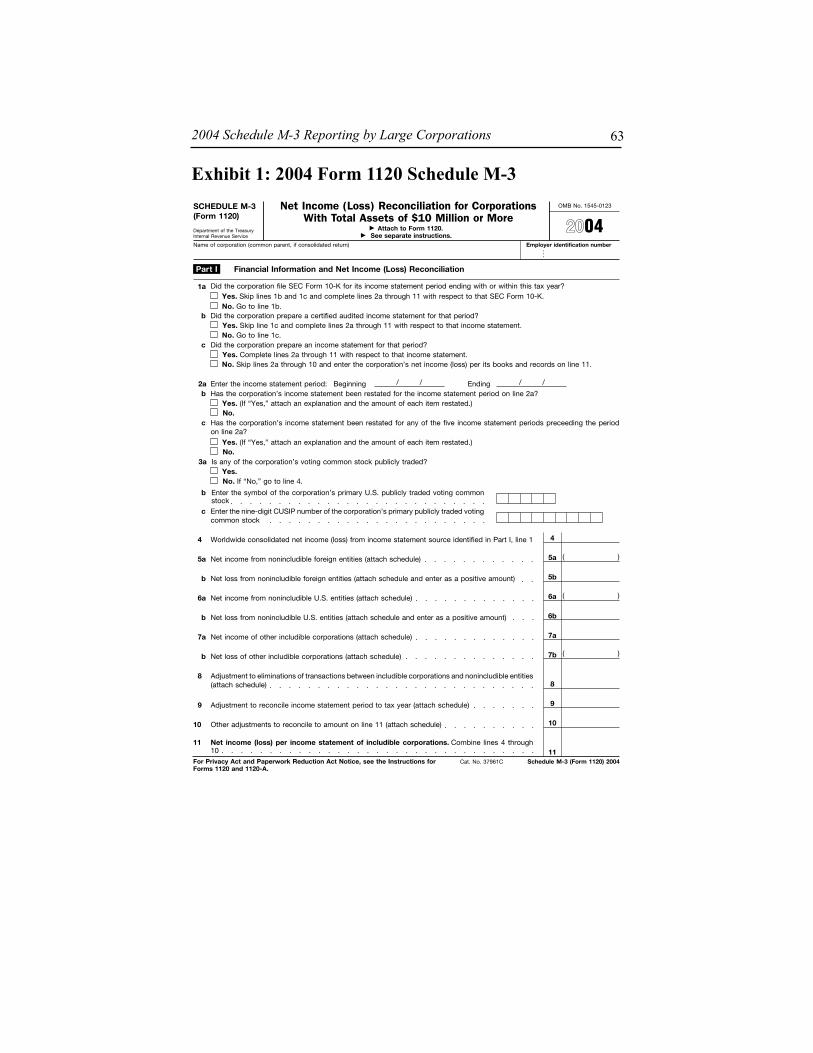
2004 Schedule M-3 Reporting by Large Corporations 63
Exhibit 1: 2004 Form 1120 Schedule M-3OMB No. 1545-0123SCHEDULE M-3 Net Income (Loss) Reconciliation for Corporations
With Total Assets of $10 Million or More(Form 1120)� Attach to Form 1120.Department of the Treasury
Internal Revenue Service
Name of corporation (common parent, if consolidated return) Employer identification number
Financial Information and Net Income (Loss) Reconciliation
Schedule M-3 (Form 1120) 2004For Privacy Act and Paperwork Reduction Act Notice, see the Instructions forForms 1120 and 1120-A.
Cat. No. 37961C
Part I
04
Did the corporation file SEC Form 10-K for its income statement period ending with or within this tax year?
b
c
Yes. Skip lines 1b and 1c and complete lines 2a through 11 with respect to that SEC Form 10-K.No. Go to line 1b.
1a
2ab
3a
Enter the income statement period: Beginning / EndingHas the corporation’s income statement been restated for the income statement period on line 2a?
Yes. (If “Yes,” attach an explanation and the amount of each item restated.)No.
Is any of the corporation’s voting common stock publicly traded?
Enter the nine-digit CUSIP number of the corporation’s primary publicly traded votingcommon stock
/ / /
4
5a
6a
7a
8
10
Worldwide consolidated net income (loss) from income statement source identified in Part I, line 1
11
Net income from nonincludible foreign entities (attach schedule)
Net income from nonincludible U.S. entities (attach schedule)
Net income of other includible corporations (attach schedule)
Adjustment to eliminations of transactions between includible corporations and nonincludible entities(attach schedule)
Other adjustments to reconcile to amount on line 11 (attach schedule)
Net income (loss) per income statement of includible corporations. Combine lines 4 through10
4
5a
6a
7a
8
10
11
� See separate instructions.
9 Adjustment to reconcile income statement period to tax year (attach schedule) 9
Did the corporation prepare a certified audited income statement for that period?Yes. Skip line 1c and complete lines 2a through 11 with respect to that income statement.No. Go to line 1c.
Did the corporation prepare an income statement for that period?Yes. Complete lines 2a through 11 with respect to that income statement.No. Skip lines 2a through 10 and enter the corporation’s net income (loss) per its books and records on line 11.
b
b Net loss from nonincludible foreign entities (attach schedule and enter as a positive amount)
b Net loss from nonincludible U.S. entities (attach schedule and enter as a positive amount)
5b
6b
Enter the symbol of the corporation’s primary U.S. publicly traded voting commonstock
c Has the corporation’s income statement been restated for any of the five income statement periods preceeding the periodon line 2a?
Yes. (If “Yes,” attach an explanation and the amount of each item restated.)No.
Yes.No. If “No,” go to line 4.
c
b Net loss of other includible corporations (attach schedule) 7b
( )
( )
( )
Exhibit 1: 2004 Form 1120 Schedule M-3

Boynton, Legel, and DeFilippes64
Page 2Schedule M-3 (Form 1120) 2004
Income (Loss) Items(d)
Income (Loss) perTax Return(optional)
(c)PermanentDifference
(b)TemporaryDifference
(a)Income (Loss) perIncome Statement
(optional)
Income (loss) from equity method foreign corporations1Gross foreign dividends not previously taxed2Subpart F, QEF, and similar income inclusions3Section 78 gross-up4Gross foreign distributions previously taxed5Income (loss) from equity method U.S. corporations6U.S. dividends not eliminated in tax consolidation7Minority interest for includible corporations8Income (loss) from U.S. partnerships (attach schedule)9Income (loss) from foreign partnerships (attach schedule)10
Income (loss) from other pass-through entities(attach schedule)Items relating to reportable transactions (attach details)
11
1213 Interest income14
Hedging transactions16 Mark-to-market income (loss)17 Inventory valuation adjustments181920
Sale versus lease (for sellers and/or lessors)Section 481(a) adjustments
21Unearned/deferred revenue
22Income recognition from long-term contractsOriginal issue discount and other imputed interest
Reconciliation of Net Income (Loss) per Income Statement of Includible Corporations WithTaxable Income per Return
Schedule M-3 (Form 1120) 2004
Total accrual to cash adjustment15
Part II
Name of corporation (common parent, if consolidated return) Employer identification number
Name of subsidiary (if consolidated return) Employer identification number
27
29
30
Other income (loss) and expense/deductionitems with no differences
Total income (loss) items. Combine lines 1through 26
Total expense/deduction items (from Part III,line 36)
Reconciliation totals. Combine lines 27 through 29
Note. Line 30, column (a), must equal the amount on Part I, line 11, and column (d) must equal Form 1120, page 1, line 28.
28
23a
23b
23c
Gross capital gains from Schedule D, excludingamounts from flow-through entities
23e
Gross capital losses from Schedule D, excludingamounts from flow-through entities, abandonmentlosses, and worthless stock losses
23f
Income statement gain/loss on sale, exchange,abandonment, worthlessness, or other disposition ofassets other than inventory and flow-through entities
23d
23g
Net gain/loss reported on Form 4797, line 17,excluding amounts from flow-through entities,abandonment losses, and worthless stock losses
Worthless stock losses (attach details)
Other gain/loss on disposition of assets other than inventory
Abandonment losses
242526 Other income (loss) items with differences (attach schedule)
Disallowed capital loss in excess of capital gainsUtilization of capital loss carryforward
Exhibit 1: 2004 Form 1120 Schedule M-3 (continued)

2004 Schedule M-3 Reporting by Large Corporations 65
Page 3Schedule M-3 (Form 1120) 2004
Expense/Deduction Items(d)
Deduction perTax Return(optional)
(c)PermanentDifference
(b)TemporaryDifference
(a)Expense per
Income Statement(optional)
Reconciliation of Net Income (Loss) per Income Statement of Includible Corporations With TaxableIncome per Return—Expense/Deduction Items
Schedule M-3 (Form 1120) 2004
12345
6789
10111213141516171819
20212223
24
2526
28293031323334
U.S. current income tax expenseU.S. deferred income tax expenseState and local current income tax expenseState and local deferred income tax expense
Foreign current income tax expense (other thanforeign withholding taxes)Foreign deferred income tax expenseForeign withholding taxesIncentive stock optionsNonqualified stock optionsOther equity-based compensationMeals and entertainmentFines and penaltiesPunitive damagesParachute paymentsCompensation with section 162(m) limitation
Charitable contribution of cash and tangiblepropertyCharitable contribution of intangible propertyCharitable contribution limitationCharitable contribution carryforward used
Current year acquisition or reorganizationinvestment banking fees
Current year acquisition or reorganization legal andaccounting feesCurrent year acquisition/reorganization other costsAmortization/impairment of goodwill
Amortization of acquisition, reorganization, andstart-up costsOther amortization or impairment write-offs
DepletionDepreciationBad debt expenseCorporate owned life insurance premiums
Other expense/deduction items with differences(attach schedule)Total expense/deduction items. Combine lines 1through 35. Enter here and on Part II, line 28
27
Part III
Pension and profit-sharingOther post-retirement benefitsDeferred compensation
Section 198 environmental remediation costs
36
Name of corporation (common parent, if consolidated return) Employer identification number
Name of subsidiary (if consolidated return) Employer identification number
35
Purchase versus lease (for purchasers and/orlessees)
Exhibit 1: 2004 Form 1120 Schedule M-3 (continued)

Boynton, Legel, and DeFilippes66
Tabl
e 1.
U.S
. Cor
pora
tions
With
Ass
ets
of $
10 M
illio
n or
Mor
e Po
tent
ially
Sub
ject
or N
ot S
ubje
ct to
200
4 Sc
hedu
le M
-3D
olla
r am
ount
s in
mill
ions
. Tab
le a
mou
nts
may
not
add
due
to ro
undi
ng. A
dvan
ce fi
le d
ata.
Val
ues
may
diff
er fr
om fi
nal f
ile a
nd o
ffici
al S
OI P
ublic
atio
n 16
val
ues.
Ret
urns
Sum
Col %
Sum
Col %
Sum
Col %
Sum
Col %
Sum
Col %
Sum
Col %
Sum
Col %
Sum
Col %
42,1
2910
040
,137
,268
100
186,
297
100
635,
757
100
57,5
9610
060
4,46
210
054
1,65
810
020
0,17
310
0S
tatu
s35
,286
8433
,884
,164
8416
0,64
786
549,
818
8657
,375
100
604,
322
100
541,
606
100
200,
093
100
100
02,
485,
878
69,
473
538
,019
60
00
00
00
035
,386
8436
,370
,042
9017
0,12
091
587,
837
9257
,375
100
604,
322
100
541,
606
100
200,
093
100
6,74
216
3,76
7,22
79
16,1
789
47,9
198
221
014
00
530
800
All
183
027
,095
,197
6882
,678
4437
2,21
559
38,5
1167
360,
403
6033
5,86
462
91,6
3046
2004
Dec
or l
ater
154
022
,737
,395
5774
,626
4033
1,82
952
38,5
1167
360,
403
6033
5,86
462
91,6
3046
2004
Nov
or e
arlie
r10
02,
331,
876
62,
144
113
,082
20
00
00
00
0P
lace
hold
er19
02,
025,
925
55,
908
327
,305
40
00
00
00
0A
ll1,
054
37,
512,
682
1953
,259
2916
7,75
126
14,1
0024
151,
020
2513
3,99
025
57,5
5529
2004
Dec
or l
ater
882
26,
309,
401
1643
,088
2313
3,21
921
14,0
9024
150,
894
2513
3,79
025
57,5
2729
2004
Nov
or e
arlie
r11
20
768,
162
26,
827
422
,224
311
012
60
200
028
0P
lace
hold
er60
043
5,11
91
3,34
52
12,3
082
00
00
00
00
All
5,24
812
3,81
7,73
310
33,0
5318
78,9
4012
4,51
68
82,9
7114
64,5
2512
37,3
0719
2004
Dec
or l
ater
4,68
811
3,37
1,66
68
28,5
8615
70,5
6811
4,30
57
82,8
1714
64,3
7512
37,2
9619
2004
Nov
or e
arlie
r54
71
421,
495
14,
247
29,
808
221
00
154
014
90
110
Pla
ceho
lder
140
24,5
720
220
0-1
,436
00
00
00
00
0A
ll35
,644
851,
711,
656
417
,308
916
,851
347
01
10,0
672
7,27
91
13,6
817
2004
Dec
or l
ater
29,5
6370
1,46
5,70
24
14,3
468
14,2
032
470
110
,207
27,
576
113
,640
720
04 N
ov o
r ear
lier
6,07
414
245,
693
12,
961
22,
805
00
0-1
400
-297
041
0P
lace
hold
er7
026
10
10
-157
00
00
00
00
0
All
Est
imat
ed IC
DW
orld
wid
eIn
com
eB
ook
Inco
me
(Par
t II L
n 30
A)
Fed
Tax
Exp
ense
2004
Adv
ance
d (8
,14,
20)
Tota
l Ass
ets
Tax
Afte
r C
redi
tsTa
x N
et
Inco
me
2004
Dec
or l
ater
c >=
$25
0M -<
$2
.5B
d >=
$ 1
0M -<
$2
50M
2004
Nov
or e
arlie
r
Pla
ceho
lder
a >=
$25
B o
r M
ore
b >=
$2.
5B -<
$2
5 B
Sub
tota
l: P
oten
tially
sub
ject
to M
-3
Sch
edul
e M
-3 2
004
Firs
t Loo
k Ta
bles
1-1
1 V
ersi
on 3
3(B
oynt
on-D
eFili
ppes
-Leg
el) (
08 1
4 06
), ta
b =
t11
of
1

2004 Schedule M-3 Reporting by Large Corporations 67
Tabl
e 2.
U.S
. Cor
pora
tions
Pot
entia
lly S
ubje
ct to
200
4 Sc
hedu
le M
-3 W
ith R
econ
cila
ble
Dat
aD
olla
r am
ount
s in
mill
ions
. Tab
le a
mou
nts
may
not
add
due
to ro
undi
ng. A
dvan
ce fi
le d
ata.
Val
ues
may
diff
er fr
om fi
nal f
ile a
nd o
ffici
al S
OI P
ublic
atio
n 16
val
ues.
Ret
urns
Sum
Col %
Sum
Col %
Sum
Col %
Sum
Col %
Sum
Col %
Sum
Col %
Sum
Col %
Sum
Col %
35,2
8610
033
,884
,164
9316
0,64
794
549,
818
9457
,375
100
604,
322
100
541,
606
100
200,
093
100
100
02,
485,
878
79,
473
638
,019
60
00
00
00
035
,386
100
36,3
70,0
4210
017
0,12
010
058
7,83
710
057
,375
100
604,
322
100
541,
606
100
200,
093
100
M3
Dat
a30
,430
8632
,544
,249
8915
1,40
589
523,
015
8952
,698
9256
8,01
094
515,
421
9519
1,67
096
2,31
07
1,08
5,76
03
7,91
85
24,3
414
4,54
48
34,8
376
24,2
394
8,20
34
128
074
,463
040
70
1,05
60
133
01,
475
01,
946
022
00
2,41
87
179,
691
091
71
1,40
60
00
00
00
00
All
154
022
,737
,395
6374
,626
4433
1,82
956
38,5
1167
360,
403
6033
5,86
462
91,6
3046
a L3
0 R
econ
cile
s15
00
22,3
89,6
1362
71,7
6842
321,
075
5538
,129
6635
0,84
058
329,
605
6187
,810
44b
L30
Pro
blem
s4
034
7,78
21
2,85
92
10,7
542
382
19,
564
26,
259
13,
820
2A
ll88
22
6,30
9,40
117
43,0
8825
133,
219
2314
,090
2515
0,89
425
133,
790
2557
,527
29a
L30
Rec
onci
les
810
25,
781,
523
1640
,374
2412
6,45
722
10,0
4118
137,
463
2312
4,76
323
54,9
4527
b L3
0 P
robl
ems
620
452,
925
12,
425
15,
769
13,
922
712
,255
27,
309
12,
377
1c
L28
Pro
blem
s5
041
,911
025
10
887
012
60
1,17
60
1,71
80
206
0d
No
I, II
40
33,0
420
370
106
00
00
00
00
0A
ll4,
688
133,
371,
666
928
,586
1770
,568
124,
305
882
,817
1464
,375
1237
,296
19a
L30
Rec
onci
les
4,30
312
3,07
2,15
98
26,5
9916
64,6
7511
4,09
37
72,8
6712
55,1
2910
35,6
8018
b L3
0 P
robl
ems
252
119
6,35
61
1,55
71
4,96
11
206
09,
699
29,
032
21,
608
1c
L28
Pro
blem
s31
028
,273
010
90
157
06
025
10
215
08
0d
No
I, II
102
074
,879
032
10
775
00
00
00
00
0A
ll8,
822
251,
021,
378
39,
146
514
,635
233
41
12,2
072
10,7
292
9,02
15
a L3
0 R
econ
cile
s7,
943
2292
6,13
63
8,19
15
12,1
422
308
19,
515
29,
347
28,
840
4b
L30
Pro
blem
s51
71
57,3
580
691
02,
111
025
02,
660
01,
367
016
90
c L2
8 P
robl
ems
290
3,06
00
280
-40
00
310
140
120
d N
o I,
II33
31
34,8
240
235
038
60
00
00
00
00
All
6,24
618
219,
588
12,
517
11,
230
010
80
-578
0-9
920
2,34
21
a L3
0 R
econ
cile
s5,
436
1519
1,02
51
2,22
71
824
010
30
-944
0-1
,006
02,
242
1b
L30
Pro
blem
s41
61
14,9
970
170
031
90
50
355
07
010
30
c L2
8 P
robl
ems
160
520
06
017
00
011
07
0-4
0d
No
I, II
379
113
,045
011
30
690
00
00
00
00
All
14,4
9441
224,
736
12,
683
2-1
,662
028
0-1
,421
0-2
,160
02,
278
1a
L30
Rec
onci
les
11,7
8933
183,
794
12,
245
1-2
,158
024
0-1
,732
0-2
,417
02,
153
1b
L30
Pro
blem
s1,
058
316
,342
021
60
427
04
030
40
264
012
50
c L2
8 P
robl
ems
470
699
013
00
00
06
0-8
0-1
0d
No
I, II
1,60
15
23,9
010
210
069
00
00
00
00
0
Fed
Tax
Exp
ense
Pla
ceho
lder
Pot
entia
lly s
ubje
ct to
M-3
a L3
0 R
econ
cile
s
2004
Dec
or l
ater
Boo
k In
com
e (P
art I
I Ln
30A
)Ta
x A
fter
Cre
dits
Tax
Net
In
com
eE
stim
ated
ICD
Wor
ldw
ide
Inco
me
2004
Adv
ance
d (8
,14,
20)
Tota
l Ass
ets
b L3
0 P
robl
ems
c L2
8 P
robl
ems
d N
o I,
IIa
>= $
25 B
or
Mor
e
f >=
$ 10
M -<
$
25M
b >=
$2.
5B -<
$2
5 B
c >=
$25
0M -<
$2
.5B
d >=
$ 5
0M -<
$2
50M
e >=
$ 2
5M -<
$
50M
Sch
edul
e M
-3 2
004
Firs
t Loo
k Ta
bles
1-1
1 V
ersi
on 3
3(B
oynt
on-D
eFili
ppes
-Leg
el) (
08 1
4 06
), ta
b =
t21
of
1

Boynton, Legel, and DeFilippes68
Tabl
e 3.
U.S
. Cor
pora
tions
Sub
ject
to 2
004
Sche
dule
M-3
With
Rec
onci
labl
e D
ata
By
Pres
ence
of 2
004
Opt
iona
l Col
umns
A a
nd D
Dat
aD
olla
r am
ount
s in
mill
ions
. Tab
le a
mou
nts
may
not
add
due
to ro
undi
ng. A
dvan
ce fi
le d
ata.
Val
ues
may
diff
er fr
om F
inal
file
and
offi
cial
SO
I Pub
licat
ion
16 v
alue
s.Pa
nel 1
of 2
Ret
urns
Pub
lic
Sum
Col %
Sum
Col %
Sum
Col %
Sum
Col %
Sum
Col %
Sum
Col %
Sum
Col %
Sum
Col %
Sum
Col %
30,4
3010
03,
922
100
32,5
44,2
4910
015
1,40
510
052
3,01
510
052
,698
100
568,
010
100
515,
421
100
191,
670
100
A &
D R
econ
15,1
6950
1,80
346
10,4
48,8
3932
56,2
5137
164,
441
3117
,133
3319
2,23
834
155,
044
3072
,796
383,
581
1228
27
1,96
2,36
56
9,78
36
35,8
667
1,56
63
42,6
058
38,1
637
11,4
236
11,6
8138
1,83
747
20,1
33,0
4562
85,3
7156
322,
708
6233
,999
6533
3,16
759
322,
214
6310
7,45
156
All
150
011
83
22,3
89,6
1369
71,7
6847
321,
075
6138
,129
7235
0,84
062
329,
605
6487
,810
46A
/D R
econ
cile
510
381
5,83
0,82
918
22,1
4515
77,7
6715
11,5
3522
101,
854
1874
,985
1527
,542
14A
/D P
robl
ems
130
90
1,13
9,45
04
4,09
33
27,5
185
746
129
,156
525
,209
54,
485
2A
/D B
lank
860
712
15,4
19,3
3547
45,5
2930
215,
790
4125
,849
4921
9,83
039
229,
411
4555
,783
29A
ll81
03
497
135,
781,
523
1840
,374
2712
6,45
724
10,0
4119
137,
463
2412
4,76
324
54,9
4529
A/D
Rec
onci
le35
31
207
52,
481,
116
815
,907
1151
,596
103,
155
648
,941
946
,171
922
,408
12A
/D P
robl
ems
620
341
432,
054
12,
378
273
20
460
15,
373
16,
145
13,
604
2A
/D B
lank
395
125
67
2,86
8,35
39
22,0
8915
74,1
3014
6,42
612
83,1
5015
72,4
4614
28,9
3315
All
4,30
314
1,58
340
3,07
2,15
99
26,5
9918
64,6
7512
4,09
38
72,8
6713
55,1
2911
35,6
8019
A/D
Rec
onci
le2,
077
774
019
1,47
4,10
95
11,7
298
27,4
125
2,22
04
34,8
056
28,1
095
15,9
928
A/D
Pro
blem
s33
51
902
254,
884
12,
140
17,
073
127
51
8,20
11
6,47
71
2,31
01
A/D
Bla
nk1,
890
675
319
1,34
3,16
64
12,7
308
30,1
896
1,59
73
29,8
625
20,5
424
17,3
779
All
7,94
326
1,10
028
926,
136
38,
191
512
,142
230
81
9,51
52
9,34
72
8,84
05
A/D
Rec
onci
le4,
075
1352
213
473,
625
14,
133
37,
741
119
80
5,72
21
6,03
31
4,51
02
A/D
Pro
blem
s77
53
782
86,8
570
668
039
00
40
465
045
10
597
0A
/D B
lank
3,09
210
501
1336
5,65
31
3,38
92
4,01
01
107
03,
328
12,
863
13,
733
2A
ll5,
436
1830
28
191,
025
12,
227
182
40
103
0-9
440
-1,0
060
2,24
21
A/D
Rec
onci
le2,
792
914
94
98,0
310
1,16
31
669
013
081
80
890
1,18
31
A/D
Pro
blem
s64
12
271
22,1
830
204
023
90
780
-617
014
00
167
0A
/D B
lank
2,00
37
126
370
,811
085
91
-83
012
0-1
,145
0-1
,235
089
20
All
11,7
8939
322
818
3,79
41
2,24
51
-2,1
580
240
-1,7
320
-2,4
170
2,15
31
A/D
Rec
onci
le5,
820
1914
74
91,1
300
1,17
21
-744
013
098
0-3
440
1,16
11
A/D
Pro
blem
s1,
754
645
126
,937
029
90
-86
03
027
0-2
600
259
0A
/D B
lank
4,21
514
130
365
,727
077
51
-1,3
280
90
-1,8
580
-1,8
130
733
0
b >=
$2.
5B -<
$2
5 B
c >=
$25
0M -<
$2
.5B
d >=
$ 5
0M -<
$2
50M
e >=
$ 2
5M -<
$
50M
All
Fed
Tax
Exp
ense
Tax
Net
In
com
eE
stim
ated
ICD
Wor
ldw
ide
Inco
me
Boo
k In
com
e (P
art I
I Ln
30A
)20
04 A
dvan
ced
(8,1
4,20
)To
tal A
sset
sTa
x A
fter
Cre
dits
A/D
Rec
onci
leA
/D P
robl
ems
A/D
Bla
nka
>= $
25 B
or
Mor
e
f >=
$ 10
M -<
$
25M
Sch
edul
e M
-3 2
004
Firs
t Loo
k Ta
bles
1-1
1 V
ersi
on 3
3(B
oynt
on-D
eFili
ppes
-Leg
el) (
08 1
4 06
), ta
b =
t31
of
2

2004 Schedule M-3 Reporting by Large Corporations 69
Tabl
e 3.
U.S
. Cor
pora
tions
Sub
ject
to 2
004
Sche
dule
M-3
With
Rec
onci
labl
e D
ata
By
Pres
ence
of 2
004
Opt
iona
l Col
umns
A a
nd D
Dat
aD
olla
r am
ount
s in
mill
ions
. Tab
le a
mou
nts
may
not
add
due
to ro
undi
ng. A
dvan
ce fi
le d
ata.
Val
ues
may
diff
er fr
om F
inal
file
and
offi
cial
SO
I Pub
licat
ion
16 v
alue
s.Pa
nel 2
of 2
Sum
Col %
Sum
Col %
Sum
Col %
Sum
Col %
Sum
Col %
Sum
Col %
Sum
Col %
Sum
Col %
Sum
Col
%70
7,09
210
0-8
1,58
710
0-5
0,13
110
057
5,37
410
0-1
31,7
1810
0-6
74,4
5110
059
2,86
410
0-3
27,9
7410
027
7,84
310
0A
& D
Rec
on22
7,84
032
-3,8
075
-42,
515
8518
1,51
932
-46,
322
35-2
20,7
0733
216,
900
37-1
17,6
5936
75,1
4427
49,5
867
-9,7
7312
-2,5
395
37,2
736
-12,
312
9-3
8,32
46
28,5
515
-23,
249
720
,710
742
9,66
661
-68,
006
83-5
,077
1035
6,58
262
-73,
083
55-4
15,4
1962
347,
413
59-1
87,0
6757
181,
989
66A
ll41
7,41
559
-28,
755
35-2
9,47
259
359,
188
62-5
8,22
744
-352
,865
5232
4,11
155
-182
,753
5615
3,28
155
A/D
Rec
onci
le10
2,52
814
23,1
58-2
8-3
6,39
273
89,2
9416
-13,
233
10-7
1,83
411
94,9
9316
-60,
564
1824
,172
9A
/D P
robl
ems
29,6
944
-3,4
974
2,06
7-4
28,2
645
-1,4
301
-12,
695
29,
198
2-9
,314
311
,381
4A
/D B
lank
285,
194
40-4
8,41
659
4,85
3-1
024
1,63
142
-43,
563
33-2
68,3
3640
219,
920
37-1
12,8
7434
117,
727
42A
ll17
9,70
825
-34,
340
42-8
,961
1813
6,40
724
-43,
301
33-1
83,4
9627
149,
156
25-8
7,40
427
78,4
4328
A/D
Rec
onci
le68
,579
10-1
3,66
017
-172
054
,748
10-1
3,83
211
-76,
855
1163
,195
11-3
1,36
010
31,1
8911
A/D
Pro
blem
s9,
750
1-4
,370
5-4
,191
81,
189
0-8
,561
6-1
5,49
62
11,1
272
-10,
523
36,
332
2A
/D B
lank
101,
379
14-1
6,31
120
-4,5
989
80,4
7014
-20,
909
16-9
1,14
514
74,8
3513
-45,
521
1440
,922
15A
ll90
,809
13-1
3,21
216
-9,0
2018
68,5
7712
-22,
232
17-9
3,14
114
79,9
2913
-42,
787
1333
,767
12A
/D R
econ
cile
44,1
026
-10,
277
13-4
,219
829
,605
5-1
4,49
711
-48,
780
738
,503
6-1
8,75
66
14,5
375
A/D
Pro
blem
s8,
787
1-1
,435
2-1
670
7,18
61
-1,6
021
-5,7
281
4,29
41
-2,3
151
2,14
81
A/D
Bla
nk37
,920
5-1
,500
2-4
,634
931
,786
6-6
,134
5-3
8,63
36
37,1
336
-21,
715
717
,082
6A
ll18
,187
3-3
,529
4-2
,214
412
,444
2-5
,744
4-3
0,15
14
26,6
224
-11,
124
38,
910
3A
/D R
econ
cile
10,5
421
-1,5
942
-1,0
122
7,93
61
-2,6
062
-15,
177
213
,583
2-4
,586
13,
575
1A
/D P
robl
ems
1,04
90
-416
1-2
390
394
0-6
550
-2,6
940
2,27
90
-753
051
40
A/D
Bla
nk6,
596
1-1
,519
2-9
632
4,11
31
-2,4
832
-12,
280
210
,760
2-5
,784
24,
821
2A
ll1,
236
0-5
531
219
090
20
-334
0-7
,466
16,
912
1-1
,381
01,
600
1A
/D R
econ
cile
1,27
30
-576
1-2
70
669
0-6
040
-3,9
261
3,35
01
-854
082
70
A/D
Pro
blem
s30
70
570
-45
031
80
120
-1,0
230
1,08
10
-192
014
60
A/D
Bla
nk-3
430
-35
029
2-1
-85
025
80
-2,5
160
2,48
20
-334
062
70
All
-263
0-1
,197
1-6
831
-2,1
440
-1,8
801
-7,3
311
6,13
51
-2,5
261
1,84
21
A/D
Rec
onci
le81
70
-857
1-6
931
-733
0-1
,550
1-4
,135
13,
278
1-1
,538
084
40
A/D
Pro
blem
s-1
0-1
140
370
-78
0-7
70
-687
057
30
-151
018
80
A/D
Bla
nk-1
,080
0-2
260
-27
0-1
,332
0-2
530
-2,5
090
2,28
40
-837
081
00
Neg
ativ
e P
reta
x P
erm
Diff
Pos
itive
Pre
tax
Per
m D
iffTa
x In
com
e (P
art I
I Ln
30D
)To
tal P
reta
x D
iffN
egat
ive
Pre
tax
Tem
p D
iffP
ositi
ve P
reta
x Te
mp
Diff
Pre
tax
Boo
kP
reta
x Te
mp
Diff
Pre
tax
Per
m
Diff
2004
Adv
ance
d (8
,14,
20)
e >=
$ 2
5M -<
$
50M
f >=
$ 10
M -<
$
25M
a >=
$25
B o
r M
ore
b >=
$2.
5B -<
$2
5 B
c >=
$25
0M -<
$2
.5B
d >=
$ 5
0M -<
$2
50M
All
A/D
Rec
onci
leA
/D P
robl
ems
A/D
Bla
nk
Sch
edul
e M
-3 2
004
Firs
t Loo
k Ta
bles
1-1
1 V
ersi
on 3
3(B
oynt
on-D
eFili
ppes
-Leg
el) (
08 1
4 06
), ta
b =
t32
of
2

Boynton, Legel, and DeFilippes70
Tabl
e 4.
U.S
. Cor
pora
tions
Sub
ject
to 2
004
Sche
dule
M-3
With
Rec
onci
labl
e D
ata
by F
inan
cial
Sta
tem
ent T
ype
Dol
lar a
mou
nts
in m
illio
ns. T
able
am
ount
s m
ay n
ot a
dd d
ue to
roun
ding
. Adv
ance
file
dat
a. V
alue
s m
ay d
iffer
from
fina
l file
and
offi
cial
SO
I Pub
licat
ion
16 v
alue
s.Pa
nel 1
of 2
Ret
urns
Pub
lic
Sum
Col %
Sum
Col %
Sum
Col %
Sum
Col %
Sum
Col %
Sum
Col %
Sum
Col %
Sum
Col %
Sum
Col %
30,4
3010
03,
922
100
32,5
44,2
4910
015
1,40
510
052
3,01
510
052
,698
100
568,
010
100
515,
421
100
191,
670
100
FS T
ype
4,19
514
3,67
394
22,2
87,3
2768
105,
533
7039
4,57
075
48,0
4691
440,
912
7841
4,12
480
140,
256
7313
,544
4517
34
5,69
5,53
318
29,1
3919
85,2
1116
1,61
03
82,2
0914
87,7
8617
33,2
3417
7,71
525
682
2,81
8,89
59
10,9
557
31,6
706
779
141
,150
7-5
580
11,9
446
4,97
616
80
1,74
2,49
35
5,77
84
11,5
632
2,26
34
3,73
81
14,0
683
6,23
63
All
150
011
83
22,3
89,6
1369
71,7
6847
321,
075
6138
,129
7235
0,84
062
329,
605
6487
,810
46a
SE
C 1
0-K
116
0*
*16
,780
,079
5259
,825
4027
5,70
653
37,4
0471
288,
075
5129
7,68
258
74,0
3839
b A
udite
d19
0*
*3,
309,
556
108,
725
635
,138
721
60
32,0
856
43,6
378
9,91
15
c U
naud
ited
90
**
1,52
9,56
55
2,65
82
10,0
092
120
28,7
395
-11,
533
-22,
869
1d
Boo
ks/R
ec6
0*
*77
0,41
32
560
022
10
497
11,
941
0-1
820
992
1A
ll81
03
497
135,
781,
523
1840
,374
2712
6,45
724
10,0
4119
137,
463
2412
4,76
324
54,9
4529
a S
EC
10-
K51
42
**
3,89
0,35
412
31,0
2820
95,5
9218
7,86
015
117,
813
2194
,891
1844
,734
23b
Aud
ited
127
0*
*75
6,78
62
4,84
83
12,5
512
646
112
,907
212
,310
25,
787
3c
Una
udite
d95
0*
*61
3,44
02
2,52
32
11,8
212
435
14,
934
15,
962
13,
341
2d
Boo
ks/R
ec75
0*
*52
0,94
22
1,97
61
6,49
41
1,10
02
1,80
90
11,5
992
1,08
31
All
4,30
314
1,58
340
3,07
2,15
99
26,5
9918
64,6
7512
4,09
38
72,8
6713
55,1
2911
35,6
8019
a S
EC
10-
K1,
745
61,
529
391,
442,
075
413
,250
927
,769
52,
701
539
,133
726
,052
519
,835
10b
Aud
ited
1,61
15
311
974,
043
38,
513
624
,873
559
11
25,1
104
21,9
294
10,0
715
c U
naud
ited
560
223
139
1,47
51
3,12
82
8,51
72
239
08,
907
26,
696
13,
167
2d
Boo
ks/R
ec38
61
00
264,
566
11,
709
13,
516
156
31
-283
045
20
2,60
71
All
7,94
326
1,10
028
926,
136
38,
191
512
,142
230
81
9,51
52
9,34
72
8,84
05
a S
EC
10-
K1,
160
498
725
157,
550
01,
303
1-2
,471
077
0-2
,082
0-2
,346
01,
502
1b
Aud
ited
4,19
514
902
481,
966
14,
771
312
,348
215
10
12,1
492
11,1
672
5,15
63
c U
naud
ited
1,56
85
201
172,
290
11,
332
190
50
690
-850
0-9
960
1,34
41
d B
ooks
/Rec
1,02
03
40
114,
330
078
51
1,36
00
120
298
01,
522
083
80
All
5,43
618
302
819
1,02
51
2,22
71
824
010
30
-944
0-1
,006
02,
242
1a
SE
C 1
0-K
317
126
67
11,3
710
840
-1,2
670
00
-1,6
080
-1,3
580
960
b A
udite
d2,
693
925
195
,099
01,
260
11,
368
03
074
60
265
01,
321
1c
Una
udite
d1,
452
58
050
,798
056
20
391
021
0-2
080
-385
047
80
d B
ooks
/Rec
974
33
033
,758
032
10
333
079
012
60
472
034
70
All
11,7
8939
322
818
3,79
41
2,24
51
-2,1
580
240
-1,7
320
-2,4
170
2,15
31
a S
EC
10-
K34
31
292
75,
898
043
0-7
580
40
-419
0-7
970
500
b A
udite
d4,
899
1622
178
,083
01,
022
1-1
,066
04
0-7
880
-1,5
220
988
1c
Una
udite
d4,
032
138
061
,328
075
10
270
40
-372
0-3
020
745
0d
Boo
ks/R
ec2,
515
80
038
,485
042
80
-360
012
0-1
530
205
037
00
f >=
$ 10
M -<
$
25M
b >=
$2.
5B -<
$2
5 B
c >=
$25
0M -<
$2
.5B
d >=
$ 5
0M -<
$2
50M
e >=
$ 2
5M -<
$
50M
b A
udite
dc
Una
udite
dd
Boo
ks/R
eca
>= $
25 B
or
Mor
e
All
a S
EC
10-
K
Wor
ldw
ide
Inco
me
Boo
k In
com
e(P
art I
I Ln
30A
)Fe
d Ta
x E
xpen
seTo
tal A
sset
sTa
x A
fter
Cre
dits
Tax
Net
In
com
eE
stim
ated
ICD
2004
Adv
ance
d (8
,14,
20)
Sch
edul
e M
-3 2
004
Firs
t Loo
k Ta
bles
1-1
1 V
ersi
on 3
3(B
oynt
on-D
eFili
ppes
-Leg
el) (
08 1
4 06
), ta
b =
t41
of
2

2004 Schedule M-3 Reporting by Large Corporations 71
Tabl
e 4.
U.S
. Cor
pora
tions
Sub
ject
to 2
004
Sche
dule
M-3
With
Rec
onci
labl
e D
ata
by F
inan
cial
Sta
tem
ent T
ype
Dol
lar a
mou
nts
in m
illio
ns. T
able
am
ount
s m
ay n
ot a
dd d
ue to
roun
ding
. Adv
ance
file
dat
a. V
alue
s m
ay d
iffer
from
fina
l file
and
offi
cial
SO
I Pub
licat
ion
16 v
alue
s.Pa
nel 2
of 2
Sum
Col %
Sum
Col %
Sum
Col %
Sum
Col %
Sum
Col %
Sum
Col %
Sum
Col %
Sum
Col %
Sum
Col %
707,
092
100
-81,
587
100
-50,
131
100
575,
374
100
-131
,718
100
-674
,451
100
592,
864
100
-327
,974
100
277,
843
100
FS T
ype
554,
380
78-7
7,51
295
-34,
507
6944
2,36
277
-112
,019
85-4
40,9
7565
363,
463
61-2
52,1
6677
217,
659
7812
1,02
017
-14,
870
18-1
9,38
039
86,7
7015
-34,
250
26-1
45,9
3222
131,
061
22-4
6,45
314
27,0
7310
11,3
862
16,0
02-2
05,
038
-10
32,4
276
21,0
41-1
6-5
1,18
68
67,1
8911
-14,
617
419
,655
720
,305
3-5
,207
6-1
,283
313
,816
2-6
,489
5-3
6,35
75
31,1
515
-14,
738
413
,455
5A
ll41
7,41
559
-28,
755
35-2
9,47
259
359,
188
62-5
8,22
744
-352
,865
5232
4,11
155
-182
,753
5615
3,28
155
a S
EC
10-
K37
1,72
053
-52,
045
64-6
,572
1331
3,10
354
-58,
618
45-2
55,6
4338
203,
598
34-1
53,3
1347
146,
741
53b
Aud
ited
53,5
498
1,81
1-2
-20,
006
4035
,354
6-1
8,19
514
-79,
221
1281
,033
14-2
3,60
77
3,60
11
c U
naud
ited
-8,6
64-1
21,9
80-2
7-3
,302
710
,014
218
,678
-14
-12,
852
234
,832
6-4
,304
11,
002
0d
Boo
ks/R
ec81
00
-501
140
9-1
718
0-9
20
-5,1
491
4,64
81
-1,5
280
1,93
71
All
179,
708
25-3
4,34
042
-8,9
6118
136,
407
24-4
3,30
133
-183
,496
2714
9,15
625
-87,
404
2778
,443
28a
SE
C 1
0-K
139,
626
20-1
7,29
021
-18,
971
3810
3,36
518
-36,
261
28-1
29,0
1319
111,
722
19-6
8,37
221
49,4
0118
b A
udite
d18
,097
3-8
,432
103,
532
-713
,197
2-4
,901
4-2
3,25
43
14,8
223
-6,1
402
9,67
23
c U
naud
ited
9,30
21
-5,6
387
8,58
8-1
712
,253
22,
950
-2-1
5,64
02
10,0
022
-3,3
921
11,9
804
d B
ooks
/Rec
12,6
822
-2,9
804
-2,1
104
7,59
31
-5,0
904
-15,
589
212
,609
2-9
,500
37,
390
3A
ll90
,809
13-1
3,21
216
-9,0
2018
68,5
7712
-22,
232
17-9
3,14
114
79,9
2913
-42,
787
1333
,767
12a
SE
C 1
0-K
45,8
876
-7,5
079
-8,0
6616
30,3
145
-15,
573
12-4
8,47
17
40,9
647
-26,
278
818
,211
7b
Aud
ited
32,0
005
-5,4
877
-1,0
832
25,4
304
-6,5
705
-24,
341
418
,854
3-1
0,32
23
9,23
93
c U
naud
ited
9,86
31
-21
0-1
,088
28,
755
2-1
,108
1-1
1,29
32
11,2
732
-4,6
261
3,53
81
d B
ooks
/Rec
3,05
90
-197
01,
217
-24,
079
11,
019
-1-9
,036
18,
839
1-1
,561
02,
777
1A
ll18
,187
3-3
,529
4-2
,214
412
,444
2-5
,744
4-3
0,15
14
26,6
224
-11,
124
38,
910
3a
SE
C 1
0-K
-843
0-6
411
-910
2-2
,394
0-1
,551
1-6
,788
16,
147
1-3
,871
12,
960
1b
Aud
ited
16,3
222
-2,6
013
-1,2
252
12,4
962
-3,8
273
-12,
680
210
,079
2-4
,388
13,
162
1c
Una
udite
d34
80
226
039
9-1
973
062
40
-7,4
291
7,65
51
-1,6
901
2,08
91
d B
ooks
/Rec
2,36
00
-513
1-4
771
1,36
90
-990
1-3
,254
02,
741
0-1
,176
069
90
All
1,23
60
-553
121
90
902
0-3
340
-7,4
661
6,91
21
-1,3
810
1,60
01
a S
EC
10-
K-1
,262
0-1
80
100
-1,2
710
-90
-684
066
60
-178
018
80
b A
udite
d1,
586
0-2
450
200
1,36
10
-225
0-3
,456
13,
210
1-5
680
588
0c
Una
udite
d94
010
030
3-1
406
031
30
-1,7
400
1,75
00
-336
063
90
d B
ooks
/Rec
819
0-3
000
-114
040
60
-413
0-1
,586
01,
286
0-2
990
185
0A
ll-2
630
-1,1
971
-683
1-2
,144
0-1
,880
1-7
,331
16,
135
1-2
,526
11,
842
1a
SE
C 1
0-K
-747
0-1
00
30
-754
0-7
0-3
770
366
0-1
540
157
0b
Aud
ited
-533
084
0-6
171
-1,0
660
-533
0-2
,978
03,
063
1-1
,429
081
10
c U
naud
ited
442
0-5
551
139
026
0-4
160
-2,2
320
1,67
80
-269
040
70
d B
ooks
/Rec
575
0-7
161
-207
0-3
490
-924
1-1
,744
01,
028
0-6
750
467
0
Neg
ativ
e P
reta
x Te
mp
Diff
Pos
itive
Pre
tax
Tem
p D
iffP
reta
x B
ook
Pos
itive
Pre
tax
Per
m D
iffP
reta
x Te
mp
Diff
Pre
tax
Per
m
Diff
Tax
Inco
me
(Par
t II L
n 30
D)
Tota
l Pre
tax
Diff
Neg
ativ
e P
reta
x P
erm
Diff
2004
Adv
ance
d (8
,14,
20)
All
a S
EC
10-
Kb
Aud
ited
c U
naud
ited
d >=
$ 5
0M -<
$2
50M
e >=
$ 2
5M -<
$
50M
f >=
$ 10
M -<
$
25M
d B
ooks
/Rec
a >=
$25
B o
r M
ore
b >=
$2.
5B -<
$2
5 B
c >=
$25
0M -<
$2
.5B S
ched
ule
M-3
200
4 Fi
rst L
ook
Tabl
es 1
-11
Ver
sion
3 3
(Boy
nton
-DeF
ilipp
es-L
egel
) (08
14
06),
tab
= t4
2 o
f 2

Boynton, Legel, and DeFilippes72
Tabl
e 5.
U.S
. Cor
pora
tions
Sub
ject
to 2
004
Sche
dule
M-3
With
Rec
onci
labl
e D
ata
by F
inan
cial
Sta
tem
ent R
esta
tem
ents
Dol
lar a
mou
nts
in m
illio
ns. T
able
am
ount
s m
ay n
ot a
dd d
ue to
roun
ding
. Adv
ance
file
dat
a. V
alue
s m
ay d
iffer
from
fina
l file
and
offi
cial
SO
I Pub
licat
ion
16 v
alue
s.Pa
nel 1
of 2
Ret
urns
Pub
lic
Sum
Col %
Sum
Col %
Sum
Col %
Sum
Col %
Sum
Col %
Sum
Col %
Sum
Col %
Sum
Col %
Sum
Col %
30,4
3010
03,
922
100
32,5
44,2
4910
015
1,40
510
052
3,01
510
052
,698
100
568,
010
100
515,
421
100
191,
670
100
Res
tate
mts
29,1
2096
3,34
785
26,3
15,9
8481
119,
990
7940
3,19
477
49,0
4593
428,
628
7541
9,03
081
150,
287
781,
150
447
512
5,72
4,44
118
29,7
3620
113,
878
222,
976
612
7,54
922
87,0
9217
36,8
4919
161
110
03
503,
824
21,
678
15,
943
167
71
11,8
332
9,29
92
4,53
52
All
150
011
83
22,3
89,6
1369
71,7
6847
321,
075
6138
,129
7235
0,84
062
329,
605
6487
,810
46N
o R
esta
tem
ent
111
084
217
,523
,064
5450
,713
3321
4,98
341
36,9
2770
225,
512
4024
8,38
348
60,2
8431
Res
tate
Prio
r 5 Y
rs o
nly
330
281
4,56
4,19
014
20,8
9214
103,
452
201,
202
211
6,51
021
75,1
2815
25,1
3313
Cur
rent
Yea
r Res
tate
60
60
302,
359
116
30
2,64
01
00
8,81
72
6,09
41
2,39
21
All
810
349
713
5,78
1,52
318
40,3
7427
126,
457
2410
,041
1913
7,46
324
124,
763
2454
,945
29N
o R
esta
tem
ent
698
240
110
4,79
5,14
915
33,2
3322
115,
987
228,
255
1612
4,98
922
111,
118
2245
,518
24R
esta
te P
rior 5
Yrs
onl
y10
00
822
839,
859
36,
193
48,
761
21,
133
210
,925
211
,922
28,
062
4C
urre
nt Y
ear R
esta
te13
013
014
6,51
50
949
11,
709
065
31
1,54
90
1,72
40
1,36
51
All
4,30
314
1,58
340
3,07
2,15
99
26,5
9918
64,6
7512
4,09
38
72,8
6713
55,1
2911
35,6
8019
No
Res
tate
men
t3,
898
131,
313
332,
751,
552
823
,906
1661
,419
123,
430
770
,828
1253
,744
1031
,915
17R
esta
te P
rior 5
Yrs
onl
y34
41
221
627
2,52
91
2,17
71
1,64
40
638
160
30
-74
03,
036
2C
urre
nt Y
ear R
esta
te60
049
148
,077
051
60
1,61
20
250
1,43
60
1,45
90
729
0A
ll7,
943
261,
100
2892
6,13
63
8,19
15
12,1
422
308
19,
515
29,
347
28,
840
5N
o R
esta
tem
ent
7,59
225
983
2588
0,91
53
7,76
35
11,8
892
306
19,
555
28,
805
28,
243
4R
esta
te P
rior 5
Yrs
onl
y30
71
101
339
,389
038
40
248
02
0-1
040
510
056
00
Cur
rent
Yea
r Res
tate
440
170
5,83
10
440
50
00
640
330
360
All
5,43
618
302
819
1,02
51
2,22
71
824
010
30
-944
0-1
,006
02,
242
1N
o R
esta
tem
ent
5,27
617
269
718
5,42
61
2,16
91
888
010
30
-754
0-8
100
2,19
71
Res
tate
Prio
r 5 Y
rs o
nly
139
023
14,
833
055
0-4
30
00
-162
0-1
850
360
Cur
rent
Yea
r Res
tate
200
100
766
03
0-2
00
00
-28
0-1
10
90
All
11,7
8939
322
818
3,79
41
2,24
51
-2,1
580
240
-1,7
320
-2,4
170
2,15
31
No
Res
tate
men
t11
,545
3829
78
179,
878
12,
206
1-1
,971
024
0-1
,503
0-2
,210
02,
129
1R
esta
te P
rior 5
Yrs
onl
y22
71
201
3,64
00
370
-183
00
0-2
230
-208
021
0C
urre
nt Y
ear R
esta
te17
04
027
60
30
-30
00
-50
10
30
f >=
$ 10
M -<
$
25M
b >=
$2.
5B -<
$2
5 B
c >=
$25
0M -<
$2
.5B
d >=
$ 5
0M -<
$2
50M
e >=
$ 2
5M -<
$
50M
No
Res
tate
men
tR
esta
te P
rior 5
Yrs
onl
yC
urre
nt Y
ear R
esta
tea
>= $
25 B
or
Mor
e
All
Fed
Tax
Exp
ense
2004
Adv
ance
d (8
,14,
20)
Tota
l Ass
ets
Tax
Afte
r C
redi
tsTa
x N
et
Inco
me
Est
imat
ed IC
DW
orld
wid
eIn
com
eB
ook
Inco
me
(Par
t II L
n 30
A)
Sch
edul
e M
-3 2
004
Firs
t Loo
k Ta
bles
1-1
1 V
ersi
on 3
3(B
oynt
on-D
eFili
ppes
-Leg
el) (
08 1
4 06
), ta
b =
t51
of
2

2004 Schedule M-3 Reporting by Large Corporations 73
Tabl
e 5.
U.S
. Cor
pora
tions
Sub
ject
to 2
004
Sche
dule
M-3
With
Rec
onci
labl
e D
ata
by F
inan
cial
Sta
tem
ent R
esta
tem
ents
Dol
lar a
mou
nts
in m
illio
ns. T
able
am
ount
s m
ay n
ot a
dd d
ue to
roun
ding
. Adv
ance
file
dat
a. V
alue
s m
ay d
iffer
from
fina
l file
and
offi
cial
SO
I Pub
licat
ion
16 v
alue
s.Pa
nel 2
of 2
Sum
Col %
Sum
Col %
Sum
Col %
Sum
Col %
Sum
Col %
Sum
Col %
Sum
Col %
Sum
Col %
Sum
Col %
707,
092
100
-81,
587
100
-50,
131
100
575,
374
100
-131
,718
100
-674
,451
100
592,
864
100
-327
,974
100
277,
843
100
Res
tate
mts
569,
316
81-7
7,22
695
-40,
176
8045
1,91
479
-117
,402
89-5
22,3
5777
445,
131
75-2
64,0
4281
223,
865
8112
3,94
118
4,06
9-5
-11,
170
2211
6,84
120
-7,1
005
-133
,141
2013
7,21
023
-57,
368
1746
,198
1713
,834
2-8
,430
101,
215
-26,
619
1-7
,215
5-1
8,95
33
10,5
232
-6,5
642
7,78
03
All
417,
415
59-2
8,75
535
-29,
472
5935
9,18
862
-58,
227
44-3
52,8
6552
324,
111
55-1
82,7
5356
153,
281
55N
o R
esta
tem
ent
308,
668
44-3
5,79
044
-20,
984
4225
1,89
444
-56,
774
43-2
67,9
1540
232,
125
39-1
40,0
8443
119,
101
43R
esta
te P
rior 5
Yrs
onl
y10
0,26
114
14,1
40-1
7-9
,747
1910
4,65
418
4,39
3-3
-72,
604
1186
,743
15-4
0,35
112
30,6
0411
Cur
rent
Yea
r Res
tate
8,48
61
-7,1
059
1,25
8-3
2,64
00
-5,8
464
-12,
347
25,
242
1-2
,317
13,
576
1A
ll17
9,70
825
-34,
340
42-8
,961
1813
6,40
724
-43,
301
33-1
83,4
9627
149,
156
25-8
7,40
427
78,4
4328
No
Res
tate
men
t15
6,63
522
-24,
386
30-8
,098
1612
4,15
122
-32,
485
25-1
35,7
2420
111,
338
19-7
2,38
722
64,2
8923
Res
tate
Prio
r 5 Y
rs o
nly
19,9
843
-9,0
4211
-1,0
482
9,89
42
-10,
090
8-4
3,14
56
34,1
046
-11,
837
410
,789
4C
urre
nt Y
ear R
esta
te3,
089
0-9
121
185
02,
362
0-7
271
-4,6
271
3,71
51
-3,1
801
3,36
51
All
90,8
0913
-13,
212
16-9
,020
1868
,577
12-2
2,23
217
-93,
141
1479
,929
13-4
2,78
713
33,7
6712
No
Res
tate
men
t85
,659
12-1
2,20
215
-8,7
8418
64,6
7411
-20,
986
16-7
6,90
311
64,7
0111
-37,
495
1128
,711
10R
esta
te P
rior 5
Yrs
onl
y2,
962
0-5
671
-128
02,
267
0-6
951
-14,
562
213
,995
2-4
,402
14,
274
2C
urre
nt Y
ear R
esta
te2,
187
0-4
431
-108
01,
636
0-5
510
-1,6
760
1,23
30
-890
078
10
All
18,1
873
-3,5
294
-2,2
144
12,4
442
-5,7
444
-30,
151
426
,622
4-1
1,12
43
8,91
03
No
Res
tate
men
t17
,048
2-3
,034
4-1
,827
412
,187
2-4
,861
4-2
7,43
84
24,4
044
-10,
262
38,
435
3R
esta
te P
rior 5
Yrs
onl
y1,
071
0-5
301
-288
125
20
-819
1-2
,442
01,
912
0-7
090
421
0C
urre
nt Y
ear R
esta
te69
035
0-9
90
50
-64
0-2
700
306
0-1
530
540
All
1,23
60
-553
121
90
902
0-3
340
-7,4
661
6,91
21
-1,3
810
1,60
01
No
Res
tate
men
t1,
387
0-6
221
201
096
60
-421
0-7
,200
16,
578
1-1
,322
01,
523
1R
esta
te P
rior 5
Yrs
onl
y-1
490
680
380
-43
010
60
-249
031
70
-37
074
0C
urre
nt Y
ear R
esta
te-2
01
0-2
00
-21
0-1
90
-17
017
0-2
20
20
All
-263
0-1
,197
1-6
831
-2,1
440
-1,8
801
-7,3
311
6,13
51
-2,5
261
1,84
21
No
Res
tate
men
t-8
10
-1,1
911
-685
1-1
,957
0-1
,877
1-7
,177
15,
986
1-2
,491
11,
805
1R
esta
te P
rior 5
Yrs
onl
y-1
870
00
30
-183
04
0-1
380
139
0-3
20
360
Cur
rent
Yea
r Res
tate
40
-60
-10
-30
-70
-16
010
0-3
01
0
e >=
$ 2
5M -<
$
50M
f >=
$ 10
M -<
$
25M
a >=
$25
B o
r M
ore
b >=
$2.
5B -<
$2
5 B
c >=
$25
0M -<
$2
.5B
d >=
$ 5
0M -<
$2
50M
All
No
Res
tate
men
tR
esta
te P
rior 5
Yrs
onl
yC
urre
nt Y
ear R
esta
te
Neg
ativ
e P
reta
x P
erm
Diff
Pos
itive
Pre
tax
Per
m D
iffTa
x In
com
e (P
art I
I Ln
30D
)To
tal P
reta
x D
iffN
egat
ive
Pre
tax
Tem
p D
iffP
ositi
ve P
reta
x Te
mp
Diff
Pre
tax
Boo
kP
reta
x Te
mp
Diff
Pre
tax
Per
m
Diff
2004
Adv
ance
d (8
,14,
20)
Sch
edul
e M
-3 2
004
Firs
t Loo
k Ta
bles
1-1
1 V
ersi
on 3
3(B
oynt
on-D
eFili
ppes
-Leg
el) (
08 1
4 06
), ta
b =
t52
of
2

Boynton, Legel, and DeFilippes74
Tabl
e 6.
U.S
. Cor
pora
tions
Sub
ject
to 2
004
Sche
dule
M-3
With
Rec
onci
labl
e D
ata
by In
dust
ryD
olla
r am
ount
s in
mill
ions
. Tab
le a
mou
nts
may
not
add
due
to ro
undi
ng. A
dvan
ce fi
le d
ata.
Val
ues
may
diff
er fr
om fi
nal f
ile a
nd o
ffici
al S
OI P
ublic
atio
n 16
val
ues.
Pane
l 1 o
f 2
Ret
urns
Pub
lic
Sum
Col %
Sum
Col %
Sum
Col %
Sum
Col %
Sum
Col %
Sum
Col %
Sum
Col %
Sum
Col %
Sum
Col %
30,4
3010
03,
922
100
32,5
44,2
4910
015
1,40
510
052
3,01
510
052
,698
100
568,
010
100
515,
421
100
191,
670
100
SO
I Div
Cd
6,35
121
1,09
528
7,26
9,59
122
48,6
1532
232,
670
4411
,475
2225
5,82
845
282,
629
5560
,319
317,
882
2686
122
7,32
1,84
422
21,4
8814
58,7
4011
2,47
65
61,6
2011
47,9
319
25,3
6713
1,77
26
372
91,
900,
420
68,
937
610
,206
213
,628
26-3
,980
-1-3
,544
-111
,025
697
63
174
41,
574,
761
56,
600
44,
658
12,
706
544
,940
82,
006
010
,861
613
,450
441,
418
3614
,477
,633
4465
,764
4321
6,74
141
22,4
1443
209,
602
3718
6,39
936
84,0
9744
All
150
011
83
22,3
89,6
1369
71,7
6847
321,
075
6138
,129
7235
0,84
062
329,
605
6487
,810
46a.
Man
ufac
turin
g38
030
14,
803,
038
1526
,018
1716
2,72
831
3,91
37
170,
166
3021
6,31
142
26,2
7014
b. F
inan
ce30
015
05,
057,
784
169,
219
636
,173
772
81
36,9
227
27,7
295
11,2
736
c. In
form
atio
n15
0*
*1,
150,
614
43,
740
212
,429
213
,298
25-2
,331
0-2
,702
-14,
727
2d.
Util
ities
/Tra
nspo
190
**
800,
199
22,
965
23,
687
11,
436
336
,660
6-4
460
6,14
83
e. A
ll O
ther
480
421
10,5
77,9
7833
29,8
2620
106,
058
2018
,754
3610
9,42
319
88,7
1217
39,3
9121
All
810
349
713
5,78
1,52
318
40,3
7427
126,
457
2410
,041
1913
7,46
324
124,
763
2454
,945
29a.
Man
ufac
turin
g21
41
138
41,
505,
111
513
,044
950
,737
105,
438
1066
,916
1254
,184
1121
,173
11b.
Fin
ance
183
168
21,
227,
563
45,
105
313
,685
31,
105
212
,738
212
,666
26,
652
3c.
Info
rmat
ion
620
**
473,
960
13,
223
23,
812
159
049
90
3,01
21
3,54
82
d. U
tiliti
es/T
rans
po67
0*
*60
1,39
82
2,06
61
-793
01,
205
23,
255
1-6
010
2,41
41
e. A
ll O
ther
284
119
05
1,97
3,49
16
16,9
3511
59,0
1611
2,23
54
54,0
5510
55,5
0211
21,1
5811
All
4,30
314
1,58
340
3,07
2,15
99
26,5
9918
64,6
7512
4,09
38
72,8
6713
55,1
2911
35,6
8019
a. M
anuf
actu
ring
921
338
710
691,
658
26,
107
417
,587
31,
985
418
,975
312
,751
28,
983
5b.
Fin
ance
996
327
07
689,
707
24,
677
310
,293
252
31
14,4
803
9,69
22
5,33
03
c. In
form
atio
n25
21
136
320
4,93
91
1,33
21
-4,4
79-1
265
1-1
,021
0-2
,793
-12,
180
1d.
Util
ities
/Tra
nspo
156
170
213
7,02
60
1,12
91
1,07
30
650
3,84
51
2,15
50
1,72
91
e. A
ll O
ther
1,97
87
721
181,
348,
829
413
,355
940
,201
81,
254
236
,588
633
,324
617
,458
9A
ll7,
943
261,
100
2892
6,13
63
8,19
15
12,1
422
308
19,
515
29,
347
28,
840
5a.
Man
ufac
turin
g1,
663
534
89
191,
611
12,
378
22,
930
111
90
1,48
70
948
02,
776
1b.
Fin
ance
2,13
97
319
824
7,12
71
1,53
71
1,12
30
350
584
084
80
1,24
91
c. In
form
atio
n41
51
113
348
,131
036
50
-646
00
0-7
90
-71
030
60
d. U
tiliti
es/T
rans
po21
41
221
24,4
700
280
050
70
00
739
066
00
381
0e.
All
Oth
er3,
512
1229
98
414,
796
13,
631
28,
228
215
40
6,78
41
6,96
31
4,12
92
All
5,43
618
302
819
1,02
51
2,22
71
824
010
30
-944
0-1
,006
02,
242
1a.
Man
ufac
turin
g1,
141
492
240
,310
059
30
370
150
-178
0-2
660
609
0b.
Fin
ance
1,50
85
972
52,9
200
433
0-7
680
780
-2,2
090
-1,7
280
410
0c.
Info
rmat
ion
336
130
111
,708
014
00
-108
00
0-1
030
-104
015
50
d. U
tiliti
es/T
rans
po17
31
60
6,18
00
890
123
00
011
80
173
010
80
e. A
ll O
ther
2,27
77
772
79,9
080
972
11,
540
09
01,
428
092
00
961
1A
ll11
,789
3932
28
183,
794
12,
245
1-2
,158
024
0-1
,732
0-2
,417
02,
153
1a.
Man
ufac
turin
g2,
373
810
23
37,8
630
476
0-1
,350
04
0-1
,538
0-1
,298
050
90
b. F
inan
ce3,
025
1093
246
,742
051
70
-1,7
660
80
-894
0-1
,276
045
40
c. In
form
atio
n69
32
341
11,0
690
136
0-8
010
50
-946
0-8
870
109
0d.
Util
ities
/Tra
nspo
347
14
05,
489
071
062
00
032
30
650
820
e. A
ll O
ther
5,35
118
892
82,6
320
1,04
51
1,69
80
70
1,32
40
979
01,
000
1
d >=
$ 5
0M -<
$2
50M
e >=
$ 2
5M -<
$
50M
f >=
$ 10
M -<
$
25M
e. A
ll O
ther
a >=
$25
B o
r M
ore
b >=
$2.
5B -<
$2
5 B
c >=
$25
0M -<
$2
.5B
a. M
anuf
actu
ring
b. F
inan
cec.
Info
rmat
ion
d. U
tiliti
es/T
rans
po
All
Fed
Tax
Exp
ense
2004
Adv
ance
d (8
,14,
20)
Tota
l Ass
ets
Tax
Afte
r C
redi
tsTa
x N
et
Inco
me
Est
imat
ed IC
DW
orld
wid
eIn
com
eB
ook
Inco
me
(Par
t II L
n 30
A)
Sch
edul
e M
-3 2
004
Firs
t Loo
k Ta
bles
1-1
1 V
ersi
on 3
3(B
oynt
on-D
eFili
ppes
-Leg
el) (
08 1
4 06
), ta
b =
t61
of
2

2004 Schedule M-3 Reporting by Large Corporations 75
Tabl
e 6.
U.S
. Cor
pora
tions
Sub
ject
to 2
004
Sche
dule
M-3
With
Rec
onci
labl
e D
ata
by In
dust
ryD
olla
r am
ount
s in
mill
ions
. Tab
le a
mou
nts
may
not
add
due
to ro
undi
ng. A
dvan
ce fi
le d
ata.
Val
ues
may
diff
er fr
om fi
nal f
ile a
nd o
ffici
al S
OI P
ublic
atio
n 16
val
ues.
Pane
l 2 o
f 2
Sum
Col %
Sum
Col %
Sum
Col %
Sum
Col %
Sum
Col %
Sum
Col %
Sum
Col %
Sum
Col %
Sum
Col %
707,
092
100
-81,
587
100
-50,
131
100
575,
374
100
-131
,718
100
-674
,451
100
592,
864
100
-327
,974
100
277,
843
100
SO
I Div
Cd
342,
948
49-2
9,09
336
-69,
716
139
244,
139
42-9
8,81
075
-249
,879
3722
0,78
537
-187
,704
5711
7,98
742
73,2
9810
-4,8
976
-7,3
7115
61,0
3111
-12,
267
9-7
1,97
911
67,0
8211
-26,
946
819
,575
77,
481
1-4
,531
620
,879
-42
23,8
294
16,3
49-1
2-7
9,46
712
74,9
3613
-26,
549
847
,428
1712
,868
2-3
,093
4-2
,415
57,
359
1-5
,508
4-7
7,03
811
73,9
4512
-19,
804
617
,389
627
0,49
638
-39,
973
498,
492
-17
239,
016
42-3
1,48
124
-196
,088
2915
6,11
526
-66,
971
2075
,464
27A
ll41
7,41
559
-28,
755
35-2
9,47
259
359,
188
62-5
8,22
744
-352
,865
5232
4,11
155
-182
,753
5615
3,28
155
a. M
anuf
actu
ring
242,
581
34-1
8,79
723
-57,
143
114
166,
641
29-7
5,94
058
-158
,593
2413
9,79
524
-125
,719
3868
,576
25b.
Fin
ance
39,0
036
1,01
1-1
-3,1
216
36,8
936
-2,1
092
-27,
705
428
,717
5-1
0,00
43
6,88
32
c. In
form
atio
n2,
026
0-2
,676
326
,377
-53
25,7
274
23,7
01-1
8-3
8,54
36
35,8
666
-7,8
742
34,2
5112
d. U
tiliti
es/T
rans
po5,
703
14,
324
-5-4
,903
105,
123
1-5
790
-38,
872
643
,195
7-9
,515
34,
612
2e.
All
Oth
er12
8,10
318
-12,
616
159,
317
-19
124,
804
22-3
,299
3-8
9,15
313
76,5
3713
-29,
640
938
,958
14A
ll17
9,70
825
-34,
340
42-8
,961
1813
6,40
724
-43,
301
33-1
83,4
9627
149,
156
25-8
7,40
427
78,4
4328
a. M
anuf
actu
ring
75,3
5711
-8,9
8611
-10,
196
2056
,175
10-1
9,18
215
-53,
775
844
,789
8-4
0,95
412
30,7
5811
b. F
inan
ce19
,318
3-3
,002
4-1
,527
314
,788
3-4
,529
3-1
9,43
63
16,4
343
-7,6
632
6,13
62
c. In
form
atio
n6,
560
1-1
,730
2-9
622
3,86
81
-2,6
922
-24,
585
422
,855
4-1
0,19
53
9,23
33
d. U
tiliti
es/T
rans
po1,
813
0-3
,757
52,
352
-540
80
-1,4
051
-27,
041
423
,284
4-8
,908
311
,260
4e.
All
Oth
er76
,660
11-1
6,86
521
1,37
2-3
61,1
6711
-15,
493
12-5
8,65
99
41,7
947
-19,
684
621
,057
8A
ll90
,809
13-1
3,21
216
-9,0
2018
68,5
7712
-22,
232
17-9
3,14
114
79,9
2913
-42,
787
1333
,767
12a.
Man
ufac
turin
g21
,734
3-9
931
-1,1
652
19,5
763
-2,1
582
-25,
703
424
,711
4-1
6,04
15
14,8
765
b. F
inan
ce15
,022
2-2
,691
3-1
,673
310
,658
2-4
,364
3-1
4,89
12
12,2
002
-5,5
202
3,84
71
c. In
form
atio
n-6
130
269
0-3
,870
8-4
,214
-1-3
,602
3-1
1,55
62
11,8
252
-6,7
442
2,87
31
d. U
tiliti
es/T
rans
po3,
884
1-2
,859
411
30
1,13
80
-2,7
462
-9,1
541
6,29
51
-1,1
490
1,26
20
e. A
ll O
ther
50,7
827
-6,9
389
-2,4
245
41,4
207
-9,3
627
-31,
836
524
,898
4-1
3,33
24
10,9
094
All
18,1
873
-3,5
294
-2,2
144
12,4
442
-5,7
444
-30,
151
426
,622
4-1
1,12
43
8,91
03
a. M
anuf
actu
ring
3,72
31
500
-724
13,
049
1-6
741
-8,3
271
8,37
81
-3,8
241
3,10
01
b. F
inan
ce2,
097
0-2
940
-650
11,
152
0-9
441
-5,6
391
5,34
51
-2,2
661
1,61
51
c. In
form
atio
n23
50
-115
0-7
672
-647
0-8
821
-3,5
871
3,47
21
-1,5
090
742
0d.
Util
ities
/Tra
nspo
1,04
00
-496
1-3
70
507
0-5
330
-1,3
050
809
0-1
760
139
0e.
All
Oth
er11
,092
2-2
,674
3-3
50
8,38
21
-2,7
102
-11,
293
28,
619
1-3
,350
13,
315
1A
ll1,
236
0-5
531
219
090
20
-334
0-7
,466
16,
912
1-1
,381
01,
600
1a.
Man
ufac
turin
g34
30
-228
0-6
80
470
-296
0-1
,861
01,
632
0-4
220
354
0b.
Fin
ance
-1,3
180
364
025
5-1
-699
061
90
-2,0
560
2,42
10
-279
053
40
c. In
form
atio
n50
0-2
180
600
-107
0-1
580
-620
040
20
-106
016
60
d. U
tiliti
es/T
rans
po28
10
-190
030
012
10
-160
0-4
180
228
0-3
10
610
e. A
ll O
ther
1,88
10
-281
0-5
80
1,54
10
-339
0-2
,510
02,
229
0-5
420
484
0A
ll-2
630
-1,1
971
-683
1-2
,144
0-1
,880
1-7
,331
16,
135
1-2
,526
11,
842
1a.
Man
ufac
turin
g-7
890
-140
0-4
201
-1,3
490
-560
0-1
,620
01,
480
0-7
430
323
0b.
Fin
ance
-822
0-2
860
-654
1-1
,762
0-9
391
-2,2
520
1,96
60
-1,2
140
560
0c.
Info
rmat
ion
-778
0-6
00
410
-796
0-1
90
-576
051
70
-121
016
20
d. U
tiliti
es/T
rans
po14
70
-115
030
062
0-8
50
-248
013
30
-25
055
0e.
All
Oth
er1,
979
0-5
971
319
-11,
701
0-2
780
-2,6
360
2,03
90
-422
074
20
Neg
ativ
e P
reta
x P
erm
Diff
Pos
itive
Pre
tax
Per
m D
iffTa
x In
com
e (P
art I
I Ln
30D
)To
tal P
reta
x D
iffN
egat
ive
Pre
tax
Tem
p D
iffP
ositi
ve P
reta
x Te
mp
Diff
Pre
tax
Boo
kP
reta
x Te
mp
Diff
Pre
tax
Per
m
Diff
2004
Adv
ance
d (8
,14,
20)
All
a. M
anuf
actu
ring
b. F
inan
cec.
Info
rmat
ion
d. U
tiliti
es/T
rans
poe.
All
Oth
era
>= $
25 B
or
Mor
e
b >=
$2.
5B -<
$2
5 B
c >=
$25
0M -<
$2
.5B
d >=
$ 5
0M -<
$2
50M
e >=
$ 2
5M -<
$
50M
f >=
$ 10
M -<
$
25M
Sch
edul
e M
-3 2
004
Firs
t Loo
k Ta
bles
1-1
1 V
ersi
on 3
3(B
oynt
on-D
eFili
ppes
-Leg
el) (
08 1
4 06
), ta
b =
t62
of
2

Boynton, Legel, and DeFilippes76
Tabl
e 7.
Agg
rega
te 2
004
Sche
dule
M-3
Dat
a fo
r U.S
. Cor
pora
tions
With
Rec
onci
labl
e D
ata
Dol
lar a
mou
nts
in m
illio
ns. T
able
am
ount
s m
ay n
ot a
dd d
ue to
roun
ding
. Adv
ance
file
dat
a. V
alue
s m
ay d
iffer
from
fina
l file
and
offi
cial
SO
I Pub
licat
ion
16 v
alue
s.
Pane
l 1 o
f 3
Popu
latio
n O
verv
iew
Ret
urns
30,4
30To
tal A
sset
s32
,544
,249
.1Ta
x Le
ss C
redi
ts15
1,40
4.7
Tax
Net
Inco
me
523,
014.
8E
stim
ated
ICD
52,6
98.4
Oth
er S
OI A
djst
-338
.7P
art I
I Lin
e 30
Col
A57
5,37
4.5
Tax
Exe
mpt
Inte
rest
10,7
85.7
% B
ook
Part
I F
INA
NC
IAL
INFO
RM
ATI
ON
($
in m
illio
ns)
Freq
Inco
me
Neg
Pos
Inco
me
Neg
Pos
4 W
orld
wid
e co
nsol
idat
ed n
et in
com
e (lo
ss)
25,6
2656
8,00
9.7
-160
,726
.072
8,73
5.7
110.
2%-3
1.2%
141.
4%5
Inc
ome(
loss
) fr n
onin
clud
ible
fore
ign
entit
ies
3,69
9-2
04,4
69.2
-310
,115
.510
5,64
6.3
-39.
7%-6
0.2%
20.5
%6
Inc
ome(
loss
) fr n
onin
clud
ible
U.S
. ent
ities
1,63
2-8
6,53
3.8
-132
,194
.245
,660
.3-1
6.8%
-25.
6%8.
9%7
Inc
ome(
loss
) of o
ther
incl
udib
le c
orpo
ratio
ns40
63,
784.
8-2
,555
.76,
340.
50.
7%-0
.5%
1.2%
8 A
djus
tmts
to e
limin
atns
(bec
ause
of l
ines
5-7
)1,
736
184,
100.
6-1
5,79
1.8
199,
892.
435
.7%
-3.1
%38
.8%
9 A
dj to
reco
ncile
inco
me
stm
t per
iod
to ta
x yr
425
6,13
5.5
-1,8
60.9
7,99
6.4
1.2%
-0.4
%1.
6%10
Oth
er a
djus
tmts
to re
conc
ile to
am
t on
line
111,
306
33,7
22.5
-61,
678.
795
,401
.36.
5%-1
2.0%
18.5
%11
Lin
e 11
onl
y (B
ooks
and
Rec
ords
)4,
734
11,9
15.4
-14,
111.
526
,026
.92.
3%-2
.7%
5.0%
** S
UB
TOTA
L.
516,
665.
610
0.2%
** A
mou
nt to
Rec
onci
le.
-1,2
43.1
-0.2
%11
Net
inco
me
per i
ncom
e st
atem
ent o
f inc
l cor
ps30
,430
515,
422.
5-1
95,3
88.4
710,
810.
910
0.0%
%Pr
etax
Boo
kIn
com
eN
egPo
sIn
com
eN
egPo
s**
Am
ount
to R
econ
cile
.-1
.30.
0%**
Net
inco
me
per P
art I
I Lin
e 30
Col
umn
A.
515,
421.
272
.9%
** R
ever
se F
eder
al ta
x ex
pens
e.
191,
670.
427
.1%
** P
reta
x bo
ok In
com
e.
707,
091.
610
0.0%
** T
empo
rary
diff
eren
ce b
efor
e Fe
d ta
x ex
pens
e.
-81,
586.
6-6
74,4
50.6
592,
864.
0-1
1.5%
-95.
4%83
.8%
** P
erm
anen
t diff
eren
ce b
efor
e Fe
d ta
x ex
pens
e.
-50,
130.
9-3
27,9
73.9
277,
842.
9-7
.1%
-46.
4%39
.3%
** N
et ta
x in
com
e pe
r Par
t II L
ine
30 C
olum
n D
.57
5,37
4.5
81.4
%**
SO
I rem
oved
ICD
.-5
2,69
8.4
-7.5
%**
Oth
er S
OI a
djus
tmen
ts.
338.
70.
0%**
Tax
net
inco
me
repo
rted
by S
OI
.52
3,01
4.8
74.0
%
Sch
edul
e M
-3 2
004
Firs
t Loo
k Ta
bles
1-1
1 V
ersi
on 3
3(B
oynt
on-D
eFili
ppes
-Leg
el) (
08 1
4 06
), ta
b =
Sch
edul
e M
-3 2
004
Firs
t Loo
k Ta
bles
1-1
1 V
ersi
on 3
3(B
oynt
on-D
eFili
ppes
-Leg
el) (
08 1
4 06
)1
of
3

2004 Schedule M-3 Reporting by Large Corporations 77
Tabl
e 7.
Agg
rega
te 2
004
Sche
dule
M-3
Dat
a fo
r U.S
. Cor
pora
tions
With
Rec
onci
labl
e D
ata
Dol
lar a
mou
nts
in m
illio
ns. T
able
am
ount
s m
ay n
ot a
dd d
ue to
roun
ding
. Adv
ance
file
dat
a. V
alue
s m
ay d
iffer
from
fina
l file
and
offi
cial
SO
I Pub
licat
ion
16 v
alue
s.
Pane
l 2 o
f 3Pa
rt II
IN
CO
ME
ITEM
SFr
eqC
ol A
Col
BC
ol C
Col
DTo
t Diff
%PT
BN
eg B
Pos
BN
eg C
Pos
C01
Inc
ome
(loss
) fro
m e
quity
met
hod
fore
ign
corp
s88
15,
531.
7-4
,529
.7-5
,369
.1.
-9,8
98.8
-1.4
%-4
,752
.122
2.4
-7,2
68.4
1,89
9.3
02 G
ross
fore
ign
divi
dend
s no
t pre
viou
sly
taxe
d1,
072
8,08
0.4
3,75
6.2
11,4
69.6
14,6
14.3
15,2
25.8
2.2%
-2,3
02.3
6,05
8.5
-7,5
15.1
18,9
84.7
03 S
ubpa
rt F,
QE
F, a
nd s
imila
r inc
ome
incl
usio
ns1,
060
.8,
549.
625
,550
.19,
063.
334
,099
.74.
8%-2
0.0
8,56
9.6
-35.
925
,586
.004
Sec
tion
78 g
ross
-up
855
.92
5.3
26,0
02.9
8,83
8.0
26,9
28.2
3.8%
0.0
925.
3-0
.326
,003
.205
Gro
ss fo
reig
n di
strib
utio
ns p
revi
ousl
y ta
xed
214
2,54
6.1
-5,0
65.8
-12,
577.
7-1
93.4
-17,
643.
5-2
.5%
-5,1
55.1
89.3
-12,
740.
316
2.6
06 I
ncom
e (lo
ss) f
rom
equ
ity m
etho
d U
.S. c
orps
1,69
431
,806
.0-9
,743
.9-3
2,43
2.8
.-4
2,17
6.7
-6.0
%-1
2,05
4.1
2,31
0.2
-37,
974.
25,
541.
507
U.S
. div
iden
ds n
ot e
limin
ated
in ta
x co
nsol
dtn
5,38
226
,293
.73,
392.
813
,666
.217
,141
.617
,058
.92.
4%-3
,224
.16,
616.
9-2
5,05
8.1
38,7
24.3
08 M
inor
ity in
tere
st fo
r inc
ludi
ble
corp
orat
ions
560
-335
.464
.363
3.0
.69
7.3
0.1%
-93.
015
7.4
-327
.096
0.0
09 I
ncom
e (lo
ss) f
rom
U.S
. par
tner
ship
s6,
151
20,1
57.5
10,8
74.7
7,98
6.3
29,6
70.3
18,8
60.9
2.7%
-23,
108.
433
,983
.0-3
,250
.011
,236
.310
Inc
ome
(loss
) fro
m fo
reig
n pa
rtner
ship
s53
21,
493.
41,
636.
2-9
2.9
2,77
0.2
1,54
3.3
0.2%
-2,3
98.2
4,03
4.4
-750
.565
7.5
11 I
ncom
e (lo
ss) f
rom
oth
er p
ass-
thro
ugh
entit
ies
934
582.
2-1
,500
.7-3
69.0
-1,1
27.7
-1,8
69.7
-0.3
%-2
,239
.973
9.1
-593
.522
4.5
12 I
tem
s re
latin
g to
repo
rtab
le tr
ansa
ctio
ns40
02,
387.
9-3
5,65
0.2
-9,1
86.4
-6,8
58.1
-44,
836.
6-6
.3%
-36,
705.
21,
055.
0-1
0,17
3.1
986.
713
Int
eres
t inc
ome
17,2
9229
6,01
9.9
-3,0
47.4
-12,
006.
024
7,83
7.1
-15,
053.
4-2
.1%
-11,
267.
28,
219.
8-1
2,97
9.7
973.
714
Tot
al a
ccru
al to
cas
h ad
just
men
t95
810
0.4
163.
95.
4-1
,363
.916
9.3
0.0%
-302
.746
6.6
-9.9
15.3
15 H
edgi
ng tr
ansa
ctio
ns70
3-6
,578
.1-2
41.5
-203
.1-5
,127
.4-4
44.6
-0.1
%-7
,798
.97,
557.
4-3
94.1
191.
016
Mar
k-to
-mar
ket i
ncom
e (lo
ss)
857
7,25
0.3
842.
4-8
58.9
-2,7
49.4
-16.
50.
0%-4
,615
.25,
457.
6-1
,008
.314
9.4
17 I
nven
tory
val
uatio
n ad
just
men
ts10
,512
-1,7
63,8
41.3
46,8
50.5
-1,2
39.4
-1,7
61,6
68.4
45,6
11.1
6.5%
-15,
243.
062
,093
.4-3
,600
.72,
361.
218
Sal
e ve
rsus
leas
e (fo
r sel
lers
and
/or l
esso
rs)
328
4,67
7.4
31,0
73.2
-1,7
49.6
15,4
25.8
29,3
23.7
4.1%
-947
.532
,020
.7-1
,769
.720
.219
Sec
tion
481(
a) a
djus
tmen
ts2,
081
.-5
40.4
28.6
-378
.6-5
11.9
-0.1
%-4
,626
.04,
085.
6-3
5.0
63.6
20 U
near
ned/
defe
rred
reve
nue
3,44
738
,519
.333
0.5
95.3
37,1
41.0
425.
80.
1%-6
,973
.67,
304.
2-1
61.4
256.
721
Inc
ome
reco
gniti
on fr
om lo
ng-te
rm c
ontra
cts
402
12,7
79.9
-22.
420
.611
,477
.4-1
.80.
0%-5
36.0
513.
6-1
.822
.422
Orig
inal
issu
e di
scou
nt &
oth
impu
ted
inte
rest
442
896.
812
4.4
-59.
574
1.1
64.9
0.0%
-2,3
79.6
2,50
4.0
-183
.212
3.6
23a
Inc
stm
t dis
post
n of
ass
ts o
ther
than
inve
ntry
14,1
6220
,718
.9-4
7,93
6.2
-7,6
64.6
.-5
5,60
0.8
-7.9
%-6
0,93
7.6
13,0
01.5
-9,8
46.1
2,18
1.4
23b
Gro
ss c
ap g
ains
Sch
D, e
xcld
ng fl
ow-th
ru e
ntit
4,26
1.
46,5
33.7
9,69
8.4
23,9
73.0
56,2
32.0
8.0%
-470
.347
,003
.9-4
27.6
10,1
26.0
23c
Gro
ss c
ap lo
sses
Sch
D, e
xcld
g flo
w-th
ru e
ntit
2,10
8.
-14,
335.
5-1
,603
.5-6
,401
.3-1
5,93
9.1
-2.3
%-1
5,18
6.5
850.
9-2
,355
.675
2.0
23d
Net
gai
n/lo
ss re
porte
d on
For
m 4
797,
line
17
15,1
21.
25,2
50.5
1,54
9.6
9,18
2.5
26,8
00.1
3.8%
-15,
424.
040
,674
.5-5
98.7
2,14
8.3
23e
Aba
ndon
men
t los
ses
740
.-2
,757
.7-4
34.0
-1,5
24.0
-3,1
91.7
-0.5
%-3
,193
.143
5.4
-455
.521
.523
f Wor
thle
ss s
tock
loss
es23
9.
-1,1
69.8
-5,6
64.4
-4,8
97.0
-6,8
34.2
-1.0
%-1
,195
.826
.0-5
,668
.44.
023
g O
th g
n/ls
s on
dis
pstn
of a
sst o
th th
an in
vntry
2,14
0.
2,94
2.9
642.
22,
015.
93,
585.
10.
5%-7
29.6
3,67
2.5
-68.
371
0.5
24 D
isal
low
ed c
apita
l los
s in
exc
ess
of c
aptl
gns
1,57
5.
13,6
12.3
3,50
7.6
7,07
4.4
17,1
19.9
2.4%
-56.
113
,668
.3-9
3.1
3,60
0.7
25 U
tiliz
atio
n of
cap
ital l
oss
carr
yfor
war
d1,
388
.-5
,746
.5-2
,521
.4-3
,155
.4-8
,267
.8-1
.2%
-5,7
83.2
36.7
-2,5
21.5
0.1
26 O
ther
inco
me
(loss
) ite
ms
with
diff
eren
ces
14,4
971,
015,
960.
7-5
8,38
3.5
-58,
508.
31,
220,
265.
9-1
16,8
91.9
-16.
5%-1
07,0
92.2
48,7
08.7
-84,
291.
225
,782
.9**
SU
BTO
T.
-274
,952
.56,
252.
1-5
1,68
5.1
-138
,213
.0-4
5,43
2.9
-6.4
%-3
56,8
10.5
363,
062.
6-2
32,1
56.2
180,
471.
2**
Am
ount
to R
econ
cile
.-6
,187
.550
4.9
-982
.7-1
66,8
26.7
-477
.8-0
.1%
-11.
651
6.5
-1,0
55.3
72.6
27 T
otal
inco
me
item
s (c
ombi
ne li
nes
1 th
ru 2
6)27
,584
-281
,140
.06,
757.
0-5
2,66
7.7
-305
,039
.8-4
5,91
0.7
-6.5
%-3
56,8
22.1
363,
579.
1-2
33,2
11.5
180,
543.
828
Tot
al e
xp/d
ed it
ems
(from
Par
t III
line
36)
29,7
12-1
,210
,065
.5-8
0,83
6.9
186,
738.
5-1
,162
,577
.4**
Exp
/Ded
bef
ore
Fed
Tax
Exp
ense
..
..
.-8
5,76
8.9
-12.
1%-3
17,1
80.6
229,
258.
7-9
4,58
5.8
96,7
38.8
29 O
ther
inc
and
exp
item
s w
ith n
o di
ffere
nces
17,8
571,
685,
039.
8.
.1,
684,
843.
3**
SU
BTO
T.
193,
834.
2-7
4,07
9.9
134,
070.
821
7,22
6.2
** A
mou
nt to
Rec
onci
le.
321,
587.
0-4
21.8
383.
735
8,14
8.3
-38.
10.
0%-4
47.9
26.2
-176
.756
0.4
30 R
econ
cilia
tion
tota
ls (c
ombi
ne li
nes
27-2
9)30
,430
515,
421.
2-7
4,50
1.6
134,
454.
557
5,37
4.5
>> R
ever
se fe
dera
l inc
ome
tax
expe
nse
.19
1,67
0.4
-7,0
85.0
-184
,585
.4.
>> P
reta
x bo
ok in
com
e an
d M
-3 d
iffer
ence
s.
707,
091.
6-8
1,58
6.6
-50,
130.
957
5,37
4.5
-131
,717
.5-1
8.6%
-674
,450
.659
2,86
4.0
-327
,973
.927
7,84
2.9
>> P
erce
nt o
f Pre
tax
book
100.
0%-1
1.5%
-7.1
%81
.4%
-18.
6%-9
5.4%
83.8
%-4
6.4%
39.3
%
Sch
edul
e M
-3 2
004
Firs
t Loo
k Ta
bles
1-1
1 V
ersi
on 3
3(B
oynt
on-D
eFili
ppes
-Leg
el) (
08 1
4 06
), ta
b =
Sch
edul
e M
-3 2
004
Firs
t Loo
k Ta
bles
1-1
1 V
ersi
on 3
3(B
oynt
on-D
eFili
ppes
-Leg
el) (
08 1
4 06
)2
of
3

Boynton, Legel, and DeFilippes78
Tabl
e 7.
Agg
rega
te 2
004
Sche
dule
M-3
Dat
a fo
r U.S
. Cor
pora
tions
With
Rec
onci
labl
e D
ata
Dol
lar a
mou
nts
in m
illio
ns. T
able
am
ount
s m
ay n
ot a
dd d
ue to
roun
ding
. Adv
ance
file
dat
a. V
alue
s m
ay d
iffer
from
fina
l file
and
offi
cial
SO
I Pub
licat
ion
16 v
alue
s.
Pane
l 3 o
f 3Pa
rt II
I EX
PEN
SE IT
EMS
(sig
n m
atch
es P
art I
I)Fr
eqC
ol A
Col
BC
ol C
Col
DTo
t Dif f
%PT
BN
eg B
Pos
BN
eg C
Pos
C01
U.S
. cur
rent
inco
me
tax
expe
nse
21,8
19-7
4,49
4.5
6,74
3.7
170,
644.
9.
177,
388.
725
.1%
-522
.27,
266.
0-1
5,95
2.1
186,
597.
002
U.S
. def
erre
d in
com
e ta
x ex
pens
e9,
701
-7,9
34.4
341.
213
,940
.5.
14,2
81.7
2.0%
-3,0
25.2
3,36
6.4
-29,
138.
643
,079
.103
Sta
te a
nd lo
cal c
urre
nt in
com
e ta
x ex
pens
e16
,855
-10,
013.
098
6.2
-649
.0-9
,934
.433
7.1
0.0%
-4,2
17.0
5,20
3.2
-2,8
78.1
2,22
9.1
04 S
tate
and
loca
l def
erre
d in
com
e ta
x ex
pens
e4,
967
-144
.5-4
05.7
42.9
.-3
62.8
-0.1
%-2
,942
.52,
536.
8-1
,394
.01,
436.
905
For
gn c
urr i
ncom
e ta
x ex
pens
e (o
ther
than
WH
)1,
342
-3,2
91.2
620.
414
,967
.8-2
72.2
15,5
88.2
2.2%
-224
.684
5.0
-803
.515
,771
.306
For
eign
def
erre
d in
com
e ta
x ex
pens
e28
1-1
03.4
-107
.919
0.3
.82
.40.
0%-2
34.3
126.
4-7
53.8
944.
107
For
eign
with
hold
ing
taxe
s92
4-6
61.2
-158
.32,
474.
8-2
00.5
2,31
6.5
0.3%
-220
.862
.5-2
09.3
2,68
4.1
08 I
ncen
tive
stoc
k op
tions
1,44
8.
-379
.1-5
,924
.7-3
,117
.8-6
,303
.8-0
.9%
-764
.138
5.0
-6,1
61.4
236.
709
Non
qual
ified
sto
ck o
ptio
ns3,
078
-1,9
48.4
-1,6
92.0
-38,
737.
9-1
7,04
5.4
-40,
430.
0-5
.7%
-4,8
23.6
3,13
1.6
-39,
061.
932
4.0
10 O
ther
equ
ity-b
ased
com
pens
atio
n1,
921
-5,2
51.7
1,69
1.0
-4,5
44.1
-6,6
31.7
-2,8
53.1
-0.4
%-2
,138
.23,
829.
2-5
,306
.776
2.6
11 M
eals
and
ent
erta
inm
ent
25,3
84-6
,585
.817
.15,
637.
0-3
,763
.95,
654.
10.
8%-1
4.4
31.5
-21.
55,
658.
512
Fin
es a
nd p
enal
ties
8,03
7-9
48.6
75.4
2,08
4.4
-93.
82,
159.
80.
3%-1
.276
.6-3
1.0
2,11
5.4
13 P
uniti
ve d
amag
es68
-54.
899
1.4
26.3
-4.4
1,01
7.7
0.1%
-7.6
999.
00.
026
.314
Par
achu
te p
aym
ents
47-2
0.1
6.7
103.
6-5
.711
0.3
0.0%
-6.6
13.3
-9.2
112.
815
Com
pens
atio
n w
ith s
ectio
n 16
2(m
) lim
itatio
n77
6-3
,433
.837
.91,
187.
3-3
,607
.41,
225.
20.
2%-2
2.4
60.3
-30.
31,
217.
616
Pen
sion
and
pro
fit-s
harin
g10
,189
-22,
284.
8-1
6,50
5.2
-1,4
66.8
-27,
560.
3-1
7,97
2.0
-2.5
%-2
6,72
5.4
10,2
20.1
-1,6
31.0
164.
217
Oth
er p
ost-r
etire
men
t ben
efits
7,47
3-1
2,61
9.7
3,59
4.7
-1,8
08.3
-10,
406.
01,
786.
40.
3%-4
,519
.88,
114.
5-1
,828
.620
.318
Def
erre
d co
mpe
nsat
ion
5,92
5-2
3,10
0.9
4,13
5.5
-189
.5-2
1,11
9.6
3,94
6.0
0.6%
-3,1
38.2
7,27
3.8
-470
.528
1.0
19 C
harit
bl c
ontri
btn
of c
ash
and
tang
ible
pro
p12
,645
-3,1
12.2
110.
0-9
99.8
-3,5
66.5
-889
.7-0
.1%
-271
.238
1.2
-1,0
66.9
67.2
20 C
harit
bl c
ontri
btn
of in
tang
ible
pro
perty
316
-137
.5-4
8.4
-78.
1-1
70.3
-126
.50.
0%-5
3.4
5.0
-80.
22.
121
Cha
ritbl
con
tribt
n lim
itatio
n8,
219
.1,
150.
852
6.6
725.
51,
677.
40.
2%-7
7.0
1,22
7.7
-2.8
529.
422
Cha
ritbl
con
tribt
n ca
rryf
orw
ard
used
2,20
4.
-667
.0-2
01.8
-234
.3-8
68.8
-0.1
%-6
73.4
6.5
-202
.00.
323
Cur
r yr a
cqst
n/re
orgn
ztn
inve
st b
ankn
g fe
es13
0-5
2.7
-77.
123
.9-6
8.0
-53.
20.
0%-1
25.0
47.8
-80.
510
4.5
24 C
urr y
r acq
stn
reor
gnzt
n le
gal+
acct
ing
fees
501
-511
.697
.537
5.8
-318
.147
3.2
0.1%
-139
.423
6.9
-21.
539
7.2
25 C
urr y
r acq
stn/
reor
gnzt
n ot
her c
osts
536
-1,0
59.2
414.
919
1.4
-691
.860
6.3
0.1%
-734
.41,
149.
3-4
15.0
606.
426
Am
ortiz
atio
n/im
pairm
ent o
f goo
dwill
5,41
4-9
,042
.5-1
1,10
7.4
9,17
9.0
-8,7
08.4
-1,9
28.3
-0.3
%-1
5,50
1.9
4,39
4.6
-1,2
70.4
10,4
49.5
27 A
mor
tizat
ion
of a
cqst
n re
org,
star
t-up
cost
s3,
985
-1,1
75.9
-450
.918
1.4
-1,6
49.6
-269
.50.
0%-1
,814
.51,
363.
6-9
3.0
274.
428
Oth
er a
mor
tizat
ion
or im
pairm
ent w
rite-
offs
12,6
30-3
3,36
5.5
31,0
65.8
19,7
99.2
-24,
259.
150
,865
.07.
2%-1
8,02
6.2
49,0
92.0
-2,4
09.3
22,2
08.5
29 S
ec 1
98 e
nviro
nmen
tal r
emed
iatio
n co
sts
197
-183
.537
9.1
-0.6
-202
.437
8.5
0.1%
-288
.866
7.9
-1.3
0.7
30 D
eple
tion
857
-4,1
93.3
2,09
8.6
-2,1
23.3
-4,5
26.2
-24.
70.
0%-2
,729
.34,
828.
0-2
,216
.793
.331
Dep
reci
atio
n26
,444
-112
,574
.6-1
13,1
62.3
384.
4-1
64,4
18.0
-112
,777
.9-1
5.9%
-130
,439
.317
,277
.0-1
91.7
576.
132
Bad
deb
t exp
ense
18,4
03-2
5,84
4.7
-6,9
03.4
-731
.1-2
8,48
7.6
-7,6
34.5
-1.1
%-1
6,81
3.5
9,91
0.1
-883
.015
1.9
33 C
orpo
rate
ow
ned
life
insu
ranc
e pr
emiu
ms
5,73
1-1
26.2
-18.
5-3
56.6
-156
.8-3
75.1
-0.1
%-1
06.7
88.2
-814
.745
8.1
34 P
urch
ase
vers
us le
ase
481
-684
.4-6
34.0
-82.
3-1
,286
.5-7
16.3
-0.1
%-1
,226
.759
2.7
-82.
70.
435
Oth
er e
xpen
se/d
edct
n ite
ms
with
diff
eren
ces
24,8
14-8
45,2
30.1
17,0
12.0
2,46
2.7
-820
,096
.019
,474
.72.
8%-7
7,94
4.5
94,9
56.6
-24,
148.
326
,611
.0**
SU
BTO
T.
-1,2
10,1
84.8
-80,
747.
418
6,53
0.4
-1,1
61,8
77.3
105,
783.
115
.0%
-320
,513
.423
9,76
6.1
-139
,661
.632
6,19
2.1
** A
mou
nt to
Rec
onci
le.
-2,8
90.8
-89.
620
7.9
-4,3
10.4
118.
40.
0%-2
14.6
125.
0-1
4.9
222.
836
Tot
exp
/ded
item
s (c
ombi
ne 1
-35
also
on
P2
2829
,709
-1,2
13,0
75.6
-80,
836.
918
6,73
8.4
-1,1
66,1
87.7
105,
901.
515
.0%
-320
,728
.023
9,89
1.1
-139
,676
.532
6,41
4.9
>> R
ever
se fe
dera
l inc
ome
tax
expe
nse
.82
,428
.9-7
,085
.0-1
84,5
85.4
.-1
91,6
70.4
-27.
1%3,
547.
4-1
0,63
2.4
45,0
90.7
-229
,676
.1>>
Par
t III
expe
nse
item
s be
fore
tax
expe
nse
.-1
,130
,646
.7-8
7,92
1.9
2,15
3.0
-1,1
66,1
87.7
-85,
768.
9-1
2.1%
-317
,180
.622
9,25
8.7
-94,
585.
896
,738
.8
Sch
edul
e M
-3 2
004
Firs
t Loo
k Ta
bles
1-1
1 V
ersi
on 3
3(B
oynt
on-D
eFili
ppes
-Leg
el) (
08 1
4 06
), ta
b =
Sch
edul
e M
-3 2
004
Firs
t Loo
k Ta
bles
1-1
1 V
ersi
on 3
3(B
oynt
on-D
eFili
ppes
-Leg
el) (
08 1
4 06
)3
of
3

2004 Schedule M-3 Reporting by Large Corporations 79
Tabl
e 8.
Agg
rega
te 2
004
Sche
dule
M-3
Dat
a fo
r U.S
. Cor
pora
tions
With
Rec
onci
labl
e D
ata:
SEC
10-
K F
inan
cial
Sta
tem
ent
Dol
lar a
mou
nts
in m
illio
ns. T
able
am
ount
s m
ay n
ot a
dd d
ue to
roun
ding
. Adv
ance
file
dat
a. V
alue
s m
ay d
iffer
from
fina
l file
and
offi
cial
SO
I Pub
licat
ion
16 v
alue
s.
Pane
l 1 o
f 3
Popu
latio
n O
verv
iew
Ret
urns
4,19
5To
tal A
sset
s22
,287
,327
.5Ta
x Le
ss C
redi
ts10
5,53
2.6
Tax
Net
Inco
me
394,
570.
1E
stim
ated
ICD
48,0
46.4
Oth
er S
OI A
djst
-254
.6P
art I
I Lin
e 30
Col
A44
2,36
1.9
Tax
Exe
mpt
Inte
rest
6,78
4.3
% B
ook
Part
I F
INA
NC
IAL
INFO
RM
ATI
ON
($
in m
illio
ns)
Freq
Inco
me
Neg
Pos
Inco
me
Neg
Pos
4 W
orld
wid
e co
nsol
idat
ed n
et in
com
e (lo
ss)
4,16
744
0,91
2.2
-107
,320
.954
8,23
3.1
106.
5%-2
5.9%
132.
4%5
Inc
ome(
loss
) fr n
onin
clud
ible
fore
ign
entit
ies
1,80
6-1
94,9
44.9
-291
,284
.496
,339
.5-4
7.1%
-70.
3%23
.3%
6 I
ncom
e(lo
ss) f
r non
incl
udib
le U
.S. e
ntiti
es78
6-7
8,75
9.1
-114
,417
.435
,658
.3-1
9.0%
-27.
6%8.
6%7
Inc
ome(
loss
) of o
ther
incl
udib
le c
orpo
ratio
ns12
42,
035.
7-1
,609
.83,
645.
40.
5%-0
.4%
0.9%
8 A
djus
tmts
to e
limin
atns
(bec
ause
of l
ines
5-7
)85
817
7,38
2.9
-14,
217.
919
1,60
0.9
42.8
%-3
.4%
46.3
%9
Adj
to re
conc
ile in
com
e st
mt p
erio
d to
tax
yr16
05,
393.
5-1
,664
.17,
057.
51.
3%-0
.4%
1.7%
10 O
ther
adj
ustm
ts to
reco
ncile
to a
mt o
n lin
e 11
607
63,2
87.1
-14,
191.
177
,478
.215
.3%
-3.4
%18
.7%
11 L
ine
11 o
nly
(Boo
ks a
nd R
ecor
ds)
2746
.3-1
88.8
235.
10.
0%0.
0%0.
1%**
SU
BTO
TAL
.41
5,35
3.6
100.
3%**
Am
ount
to R
econ
cile
.-1
,228
.8-0
.3%
11 N
et in
com
e pe
r inc
ome
stat
emen
t of i
ncl c
orps
4,19
541
4,12
4.8
-109
,509
.452
3,63
4.3
100.
0%
%Pr
etax
Boo
kIn
com
eN
egPo
s**
Am
ount
to R
econ
cile
.-0
.60.
0%**
Net
inco
me
per P
art I
I Lin
e 30
Col
umn
A.
414,
124.
274
.7%
** R
ever
se F
eder
al ta
x ex
pens
e.
140,
256.
125
.3%
** P
reta
x bo
ok In
com
e.
554,
380.
310
0.0%
** T
empo
rary
diff
eren
ce b
efor
e Fe
d ta
x ex
pens
e.
-77,
512.
0-4
40,9
75.3
363,
463.
4-1
4.0%
-79.
5%65
.6%
** P
erm
anen
t diff
eren
ce b
efor
e Fe
d ta
x ex
pens
e.
-34,
506.
9-2
52,1
66.1
217,
659.
1-6
.2%
-45.
5%39
.3%
** N
et ta
x in
com
e pe
r Par
t II L
ine
30 C
olum
n D
.44
2,36
1.9
79.8
%**
SO
I rem
oved
ICD
.-4
8,04
6.4
-8.7
%**
Oth
er S
OI a
djus
tmen
ts.
254.
60.
0%**
Tax
net
inco
me
repo
rted
by S
OI
.39
4,57
0.1
71.2
%
Sch
edul
e M
-3 2
004
Firs
t Loo
k Ta
bles
1-1
1 V
ersi
on 3
3(B
oynt
on-D
eFili
ppes
-Leg
el) (
08 1
4 06
), ta
b =
Sch
edul
e M
-3 2
004
Firs
t Loo
k Ta
bles
1-1
1 V
ersi
on 3
3(B
oynt
on-D
eFili
ppes
-Leg
el) (
08 1
4 06
)1
of
3

Boynton, Legel, and DeFilippes80
Tabl
e 8.
Agg
rega
te 2
004
Sche
dule
M-3
Dat
a fo
r U.S
. Cor
pora
tions
With
Rec
onci
labl
e D
ata:
SEC
10-
K F
inan
cial
Sta
tem
ent
Dol
lar a
mou
nts
in m
illio
ns. T
able
am
ount
s m
ay n
ot a
dd d
ue to
roun
ding
. Adv
ance
file
dat
a. V
alue
s m
ay d
iffer
from
fina
l file
and
offi
cial
SO
I Pub
licat
ion
16 v
alue
s.
Pane
l 2 o
f 3Pa
rt II
IN
CO
ME
ITEM
SFr
eqC
ol A
Col
BC
ol C
Col
DTo
t Diff
%PT
BN
eg B
Pos
BN
eg C
Pos
C01
Inc
ome
(loss
) fro
m e
quity
met
hod
fore
ign
corp
s33
24,
694.
4-4
,222
.9-4
,005
.9.
-8,2
28.8
-1.5
%-4
,363
.314
0.4
-5,4
94.8
1,48
9.0
02 G
ross
fore
ign
divi
dend
s no
t pre
viou
sly
taxe
d45
86,
059.
94,
052.
49,
767.
311
,959
.313
,819
.72.
5%-1
,381
.75,
434.
1-6
,680
.016
,447
.303
Sub
part
F, Q
EF,
and
sim
ilar i
ncom
e in
clus
ions
650
.7,
587.
523
,343
.37,
602.
630
,930
.85.
6%-6
.27,
593.
7-3
3.6
23,3
76.9
04 S
ectio
n 78
gro
ss-u
p45
8.
723.
724
,140
.87,
650.
724
,864
.54.
5%0.
072
3.7
-0.3
24,1
41.2
05 G
ross
fore
ign
dist
ribut
ions
pre
viou
sly
taxe
d13
12,
393.
5-4
,995
.2-1
2,34
5.8
-123
.3-1
7,34
1.0
-3.1
%-4
,996
.51.
3-1
2,47
0.6
124.
806
Inc
ome
(loss
) fro
m e
quity
met
hod
U.S
. cor
ps48
624
,863
.4-7
,737
.9-2
7,13
5.2
.-3
4,87
3.1
-6.3
%-9
,205
.11,
467.
2-3
1,97
3.3
4,83
8.1
07 U
.S. d
ivid
ends
not
elim
inat
ed in
tax
cons
oldt
n1,
026
6,81
1.1
2,15
9.3
23,9
12.6
10,8
26.6
26,0
71.9
4.7%
-2,4
03.6
4,56
2.9
-9,4
29.3
33,3
41.8
08 M
inor
ity in
tere
st fo
r inc
ludi
ble
corp
orat
ions
164
-206
.028
.211
4.6
.14
2.8
0.0%
-73.
610
1.7
-293
.740
8.3
09 I
ncom
e (lo
ss) f
rom
U.S
. par
tner
ship
s1,
481
9,65
3.7
8,22
5.7
7,75
3.6
16,4
32.5
15,9
79.3
2.9%
-13,
491.
521
,717
.2-1
,351
.09,
104.
610
Inc
ome
(loss
) fro
m fo
reig
n pa
rtner
ship
s26
195
4.4
-56.
819
4.5
1,84
1.9
137.
70.
0%-1
,815
.21,
758.
4-2
87.6
482.
111
Inc
ome
(loss
) fro
m o
ther
pas
s-th
roug
h en
titie
s29
329
0.8
-927
.3-2
74.6
-810
.4-1
,201
.9-0
.2%
-1,2
93.1
365.
8-4
08.1
133.
512
Ite
ms
rela
ting
to re
porta
ble
trans
actio
ns21
33,
077.
6-2
7,72
0.1
-7,1
30.5
-1,7
57.9
-34,
850.
6-6
.3%
-28,
229.
350
9.2
-8,0
32.3
901.
813
Int
eres
t inc
ome
2,83
316
9,02
7.1
-2,2
75.6
-7,6
94.3
164,
564.
1-9
,970
.0-1
.8%
-7,9
92.1
5,71
6.5
-8,4
81.4
787.
014
Tot
al a
ccru
al to
cas
h ad
just
men
t47
-916
.7-5
9.0
-7.8
-2,5
93.9
-66.
80.
0%-8
2.8
23.8
-7.8
0.0
15 H
edgi
ng tr
ansa
ctio
ns33
3-5
,953
.7-2
,163
.5-2
25.0
-3,3
78.6
-2,3
88.5
-0.4
%-5
,685
.53,
522.
0-3
88.0
163.
016
Mar
k-to
-mar
ket i
ncom
e (lo
ss)
311
8,34
2.2
257.
5-8
64.2
2,12
5.5
-606
.7-0
.1%
-2,7
23.0
2,98
0.5
-1,0
03.9
139.
617
Inv
ento
ry v
alua
tion
adju
stm
ents
1,79
8-8
90,0
42.8
2,05
6.7
-876
.3-8
80,0
17.4
1,18
0.4
0.2%
-8,9
03.8
10,9
60.5
-3,0
03.1
2,12
6.8
18 S
ale
vers
us le
ase
(for s
elle
rs a
nd/o
r les
sors
)12
11,
922.
325
,720
.5-1
8.7
8,84
5.1
25,7
01.8
4.6%
-629
.426
,350
.0-1
8.7
0.0
19 S
ectio
n 48
1(a)
adj
ustm
ents
659
.-3
42.3
1.7
-422
.9-3
40.6
-0.1
%-3
,423
.93,
081.
6-3
.35.
020
Une
arne
d/de
ferr
ed re
venu
e1,
304
21,4
46.8
-260
.213
5.5
19,8
43.6
-124
.70.
0%-5
,481
.85,
221.
5-1
16.7
252.
221
Inc
ome
reco
gniti
on fr
om lo
ng-te
rm c
ontra
cts
775,
127.
7-8
.00.
85,
124.
4-7
.10.
0%-3
58.1
350.
1-0
.71.
522
Orig
inal
issu
e di
scou
nt &
oth
impu
ted
inte
rest
182
820.
9-1
84.8
-19.
264
3.0
-204
.00.
0%-1
,801
.11,
616.
4-5
9.9
40.7
23a
Inc
stm
t dis
post
n of
ass
ts o
ther
than
inve
ntry
2,80
010
,142
.1-3
5,77
5.3
-1,2
51.9
.-3
7,02
7.1
-6.7
%-4
3,31
5.4
7,54
0.1
-2,6
29.0
1,37
7.2
23b
Gro
ss c
ap g
ains
Sch
D, e
xcld
ng fl
ow-th
ru e
ntit
1,14
9.
34,8
84.2
5,00
7.0
14,5
98.6
39,8
91.1
7.2%
-188
.535
,072
.7-2
84.0
5,29
1.0
23c
Gro
ss c
ap lo
sses
Sch
D, e
xcld
g flo
w-th
ru e
ntit
564
.-8
,593
.8-1
,571
.4-2
,682
.0-1
0,16
5.2
-1.8
%-8
,992
.839
8.9
-1,8
28.9
257.
523
d N
et g
ain/
loss
repo
rted
on F
orm
479
7, li
ne 1
73,
061
.15
,096
.298
9.1
5,67
7.2
16,0
85.2
2.9%
-9,2
41.3
24,3
37.4
-322
.61,
311.
623
e A
band
onm
ent l
osse
s27
0.
-2,1
88.4
-361
.3-1
,296
.2-2
,549
.6-0
.5%
-2,5
66.0
377.
6-3
67.2
6.0
23f W
orth
less
sto
ck lo
sses
104
.-7
95.0
-5,3
06.3
-4,4
15.5
-6,1
01.3
-1.1
%-8
17.4
22.4
-5,3
06.3
0.0
23g
Oth
gn/
lss
on d
isps
tn o
f ass
t oth
than
invn
try37
2.
1,11
8.0
95.8
555.
61,
213.
80.
2%-3
08.2
1,42
6.2
-30.
612
6.5
24 D
isal
low
ed c
apita
l los
s in
exc
ess
of c
aptl
gns
420
.8,
642.
11,
488.
51,
823.
210
,130
.61.
8%-1
4.0
8,65
6.1
-93.
01,
581.
525
Util
izat
ion
of c
apita
l los
s ca
rryf
orw
ard
304
.-4
,102
.6-1
,373
.6-1
,954
.1-5
,476
.2-1
.0%
-4,1
38.6
36.0
-1,3
73.6
0.0
26 O
ther
inco
me
(loss
) ite
ms
with
diff
eren
ces
2,82
769
1,04
4.5
-8,7
69.4
-49,
598.
671
2,43
3.9
-58,
368.
0-1
0.5%
-42,
632.
733
,863
.3-6
8,83
5.7
19,2
37.1
** S
UB
TOT
.69
,553
.0-6
26.1
-23,
115.
293
,095
.6-2
3,74
1.3
-4.3
%-2
16,5
55.3
215,
929.
3-1
70,6
09.0
147,
493.
8**
Am
ount
to R
econ
cile
.36
,965
.447
8.6
-998
.320
,880
.1-5
19.7
-0.1
%-4
.048
2.6
-1,0
54.1
55.8
27 T
otal
inco
me
item
s (c
ombi
ne li
nes
1 th
ru 2
6)4,
100
106,
518.
4-1
47.5
-24,
113.
511
3,97
5.7
-24,
261.
0-4
.4%
-216
,559
.421
6,41
1.9
-171
,663
.114
7,54
9.6
28 T
otal
exp
/ded
item
s (fr
om P
art I
II lin
e 36
)4,
185
-771
,234
.9-7
3,44
3.4
125,
920.
0-7
61,3
90.9
** E
xp/D
ed b
efor
e Fe
d Ta
x E
xpen
se.
..
..
-87,
779.
7-1
5.8%
-224
,090
.814
7,04
5.4
-80,
328.
469
,594
.129
Oth
er in
c an
d ex
p ite
ms
with
no
diffe
renc
es2,
177
808,
198.
0.
.80
8,11
8.5
** S
UB
TOT
.14
3,48
1.5
-73,
590.
910
1,80
6.5
160,
703.
3**
Am
ount
to R
econ
cile
.27
0,64
2.7
-319
.134
0.8
281,
658.
621
.70.
0%-3
25.2
6.1
-174
.551
5.3
30 R
econ
cilia
tion
tota
ls (c
ombi
ne li
nes
27-2
9)4,
195
414,
124.
2-7
3,91
0.0
102,
147.
344
2,36
1.9
>> R
ever
se fe
dera
l inc
ome
tax
expe
nse
.14
0,25
6.1
-3,6
02.0
-136
,654
.1.
>> P
reta
x bo
ok in
com
e an
d M
-3 d
iffer
ence
s.
554,
380.
3-7
7,51
2.0
-34,
506.
944
2,36
1.9
-112
,018
.8-2
0.2%
-440
,975
.336
3,46
3.4
-252
,166
.121
7,65
9.1
>> P
erce
nt o
f Pre
tax
book
100.
0%-1
4.0%
-6.2
%79
.8%
-20.
2%-7
9.5%
65.6
%-4
5.5%
39.3
%
Sch
edul
e M
-3 2
004
Firs
t Loo
k Ta
bles
1-1
1 V
ersi
on 3
3(B
oynt
on-D
eFili
ppes
-Leg
el) (
08 1
4 06
), ta
b =
Sch
edul
e M
-3 2
004
Firs
t Loo
k Ta
bles
1-1
1 V
ersi
on 3
3(B
oynt
on-D
eFili
ppes
-Leg
el) (
08 1
4 06
)2
of
3

2004 Schedule M-3 Reporting by Large Corporations 81
Tabl
e 8.
Agg
rega
te 2
004
Sche
dule
M-3
Dat
a fo
r U.S
. Cor
pora
tions
With
Rec
onci
labl
e D
ata:
SEC
10-
K F
inan
cial
Sta
tem
ent
Dol
lar a
mou
nts
in m
illio
ns. T
able
am
ount
s m
ay n
ot a
dd d
ue to
roun
ding
. Adv
ance
file
dat
a. V
alue
s m
ay d
iffer
from
fina
l file
and
offi
cial
SO
I Pub
licat
ion
16 v
alue
s.
Pane
l 3 o
f 3Pa
rt II
I EX
PEN
SE IT
EMS
(sig
n m
atch
es P
art I
I)Fr
eqC
ol A
Col
BC
ol C
Col
DTo
t Diff
%PT
BN
eg B
Pos
BN
eg C
Pos
C01
U.S
. cur
rent
inco
me
tax
expe
nse
3,23
0-5
2,17
5.7
1,93
7.3
127,
281.
2.
129,
218.
523
.3%
-276
.62,
213.
9-1
0,71
1.2
137,
992.
302
U.S
. def
erre
d in
com
e ta
x ex
pens
e1,
628
-4,7
65.7
1,66
4.7
9,37
3.0
.11
,037
.72.
0%-3
46.3
2,01
0.9
-22,
267.
131
,640
.103
Sta
te a
nd lo
cal c
urre
nt in
com
e ta
x ex
pens
e2,
935
-5,9
35.5
1,34
9.3
-952
.2-5
,869
.539
7.0
0.1%
-2,7
30.8
4,08
0.1
-2,3
85.7
1,43
3.5
04 S
tate
and
loca
l def
erre
d in
com
e ta
x ex
pens
e1,
106
110.
7-5
99.9
-194
.1.
-794
.0-0
.1%
-2,3
47.9
1,74
8.0
-1,1
06.3
912.
205
For
gn c
urr i
ncom
e ta
x ex
pens
e (o
ther
than
WH
)61
1-2
,676
.725
3.6
13,2
07.2
-105
.713
,460
.82.
4%-1
94.1
447.
7-4
26.9
13,6
34.1
06 F
orei
gn d
efer
red
inco
me
tax
expe
nse
165
-159
.4-1
75.4
302.
0.
126.
60.
0%-2
21.6
46.2
-564
.786
6.7
07 F
orei
gn w
ithho
ldin
g ta
xes
400
-478
.5-1
68.7
2,29
4.0
-137
.12,
125.
30.
4%-2
12.9
44.2
-191
.02,
485.
008
Inc
entiv
e st
ock
optio
ns1,
115
.-3
89.1
-5,6
32.8
-2,8
11.2
-6,0
21.9
-1.1
%-6
57.5
268.
4-5
,811
.217
8.4
09 N
onqu
alifi
ed s
tock
opt
ions
2,19
3-1
,598
.1-2
,069
.3-3
6,30
3.9
-16,
036.
4-3
8,37
3.1
-6.9
%-4
,472
.72,
403.
5-3
6,57
7.3
273.
410
Oth
er e
quity
-bas
ed c
ompe
nsat
ion
1,27
4-4
,340
.31,
591.
0-3
,953
.9-5
,499
.2-2
,362
.8-0
.4%
-1,7
04.3
3,29
5.3
-4,6
34.1
680.
211
Mea
ls a
nd e
nter
tain
men
t4,
013
-3,5
32.0
-5.0
3,43
5.2
-2,1
05.3
3,43
0.2
0.6%
-13.
18.
1-1
9.3
3,45
4.5
12 F
ines
and
pen
altie
s1,
887
-621
.545
.21,
719.
0-1
3.1
1,76
4.2
0.3%
-0.8
46.0
-18.
41,
737.
313
Pun
itive
dam
ages
29-2
6.1
873.
51.
0-0
.387
4.5
0.2%
-1.5
875.
00.
01.
014
Par
achu
te p
aym
ents
29-3
.76.
838
.27.
544
.90.
0%-6
.513
.30.
038
.215
Com
pens
atio
n w
ith s
ectio
n 16
2(m
) lim
itatio
n60
6-2
,269
.639
.31,
158.
1-2
,448
.11,
197.
40.
2%-1
2.6
51.9
-30.
31,
188.
516
Pen
sion
and
pro
fit-s
harin
g1,
883
-14,
211.
7-1
4,27
3.0
-1,4
07.8
-18,
511.
6-1
5,68
0.8
-2.8
%-2
2,27
6.4
8,00
3.3
-1,5
27.9
120.
117
Oth
er p
ost-r
etire
men
t ben
efits
1,23
5-6
,905
.32,
277.
8-1
,478
.6-5
,307
.379
9.2
0.1%
-3,8
41.6
6,11
9.4
-1,4
84.8
6.2
18 D
efer
red
com
pens
atio
n1,
835
-14,
705.
62,
338.
1-1
93.7
-13,
468.
72,
144.
40.
4%-2
,392
.14,
730.
3-4
03.2
209.
519
Cha
ritbl
con
tribt
n of
cas
h an
d ta
ngib
le p
rop
2,23
3-1
,939
.329
.0-8
19.3
-2,3
05.4
-790
.4-0
.1%
-221
.925
0.8
-867
.748
.320
Cha
ritbl
con
tribt
n of
inta
ngib
le p
rope
rty69
-76.
0-4
6.4
-65.
3-1
13.8
-111
.80.
0%-4
6.9
0.4
-66.
00.
721
Cha
ritbl
con
tribt
n lim
itatio
n1,
348
.75
6.8
350.
937
5.7
1,10
7.7
0.2%
-61.
281
8.0
-1.8
352.
722
Cha
ritbl
con
tribt
n ca
rryf
orw
ard
used
333
.-4
26.3
-69.
3-1
13.3
-495
.6-0
.1%
-427
.61.
3-6
9.3
0.1
23 C
urr y
r acq
stn/
reor
gnzt
n in
vest
ban
kng
fees
69-2
7.9
-34.
42.
7-4
2.8
-31.
70.
0%-7
2.0
37.6
-55.
257
.924
Cur
r yr a
cqst
n re
orgn
ztn
lega
l+ac
ctin
g fe
es22
4-3
80.9
63.6
273.
0-2
70.9
336.
60.
1%-1
17.7
181.
3-1
2.2
285.
325
Cur
r yr a
cqst
n/re
orgn
ztn
othe
r cos
ts24
5-8
26.7
330.
419
5.6
-544
.052
6.0
0.1%
-477
.180
7.5
-45.
724
1.3
26 A
mor
tizat
ion/
impa
irmen
t of g
oodw
ill1,
673
-2,5
12.5
-8,4
99.1
3,23
3.7
-4,9
85.8
-5,2
65.4
-0.9
%-1
0,64
1.7
2,14
2.6
-991
.14,
224.
827
Am
ortiz
atio
n of
acq
stn
reor
g,st
art-u
p co
sts
1,10
8-6
30.5
-264
.545
.0-7
47.6
-219
.50.
0%-9
14.9
650.
4-5
2.0
97.0
28 O
ther
am
ortiz
atio
n or
impa
irmen
t writ
e-of
fs2,
868
-23,
272.
727
,856
.218
,460
.6-1
6,10
0.2
46,3
16.8
8.4%
-12,
604.
440
,460
.6-2
,216
.920
,677
.429
Sec
198
env
ironm
enta
l rem
edia
tion
cost
s98
-130
.437
6.1
-1.2
-140
.837
4.9
0.1%
-231
.260
7.4
-1.3
0.1
30 D
eple
tion
214
-2,0
39.8
1,28
6.0
-1,1
40.4
-2,5
47.6
145.
60.
0%-2
,106
.03,
392.
0-1
,204
.163
.731
Dep
reci
atio
n4,
068
-72,
259.
3-7
4,74
4.6
363.
1-1
01,0
65.9
-74,
381.
6-1
3.4%
-86,
452.
411
,707
.8-1
18.7
481.
832
Bad
deb
t exp
ense
3,51
4-1
7,50
5.2
-3,2
23.0
-254
.0-1
9,07
7.7
-3,4
77.0
-0.6
%-9
,191
.55,
968.
5-3
24.2
70.1
33 C
orpo
rate
ow
ned
life
insu
ranc
e pr
emiu
ms
958
43.0
3.7
-458
.0-6
6.8
-454
.3-0
.1%
-34.
037
.7-7
13.6
255.
534
Pur
chas
e ve
rsus
leas
e20
6-3
94.4
-489
.9-6
5.7
-814
.4-5
55.7
-0.1
%-8
86.5
396.
5-6
6.0
0.3
35 O
ther
exp
ense
/ded
ctn
item
s w
ith d
iffer
ence
s4,
066
-535
,349
.5-1
1,00
6.3
-3,0
30.0
-541
,159
.6-1
4,03
6.4
-2.5
%-5
8,30
6.8
47,3
00.5
-18,
341.
515
,311
.4**
SU
BTO
T.
-771
,596
.9-7
3,33
6.9
125,
713.
2-7
62,0
26.9
52,3
76.3
9.4%
-224
,503
.115
1,16
6.2
-113
,306
.623
9,01
9.8
** A
mou
nt to
Rec
onci
le.
-3,8
83.7
-106
.520
6.7
-3,4
72.8
100.
20.
0%-2
10.5
104.
0-0
.120
6.7
36 T
ot e
xp/d
ed it
ems
(com
bine
1-3
5 al
so o
n P
2 28
4,18
5-7
75,4
80.6
-73,
443.
412
5,91
9.9
-765
,499
.752
,476
.49.
5%-2
24,7
13.7
151,
270.
2-1
13,3
06.6
239,
226.
5>>
Rev
erse
fede
ral i
ncom
e ta
x ex
pens
e.
56,9
41.5
-3,6
02.0
-136
,654
.1.
-140
,256
.1-2
5.3%
622.
9-4
,224
.932
,978
.2-1
69,6
32.4
>> P
art I
II ex
pens
e ite
ms
befo
re ta
x ex
pens
e.
-718
,539
.1-7
7,04
5.4
-10,
734.
3-7
65,4
99.7
-87,
779.
7-1
5.8%
-224
,090
.814
7,04
5.4
-80,
328.
469
,594
.1
Sch
edul
e M
-3 2
004
Firs
t Loo
k Ta
bles
1-1
1 V
ersi
on 3
3(B
oynt
on-D
eFili
ppes
-Leg
el) (
08 1
4 06
), ta
b =
Sch
edul
e M
-3 2
004
Firs
t Loo
k Ta
bles
1-1
1 V
ersi
on 3
3(B
oynt
on-D
eFili
ppes
-Leg
el) (
08 1
4 06
)3
of
3

Boynton, Legel, and DeFilippes82
Tabl
e 9.
Agg
rega
te 2
004
Sche
dule
M-3
Dat
a fo
r U.S
. Cor
pora
tions
With
Rec
onci
labl
e D
ata:
Aud
ited
Fina
ncia
l Sta
tem
ent (
Not
SEC
10-
K)
Dol
lar a
mou
nts
in m
illio
ns. T
able
am
ount
s m
ay n
ot a
dd d
ue to
roun
ding
. Adv
ance
file
dat
a. V
alue
s m
ay d
iffer
from
fina
l file
and
offi
cial
SO
I Pub
licat
ion
16 v
alue
s.
Pane
l 1 o
f 3
Popu
latio
n O
verv
iew
Ret
urns
13,5
44To
tal A
sset
s5,
695,
533.
2Ta
x Le
ss C
redi
ts29
,138
.8Ta
x N
et In
com
e85
,210
.9E
stim
ated
ICD
1,61
0.0
Oth
er S
OI A
djst
-50.
6P
art I
I Lin
e 30
Col
A86
,770
.3Ta
x E
xem
pt In
tere
st1,
958.
0%
Boo
kPa
rt I
FIN
AN
CIA
L IN
FOR
MA
TIO
N (
$ in
mill
ions
)Fr
eqIn
com
eN
egPo
sIn
com
eN
egPo
s4
Wor
ldw
ide
cons
olid
ated
net
inco
me
(loss
)13
,344
82,2
08.8
-27,
883.
311
0,09
2.1
93.6
%-3
1.8%
125.
4%5
Inc
ome(
loss
) fr n
onin
clud
ible
fore
ign
entit
ies
1,50
1-8
,360
.4-1
2,26
7.3
3,90
6.8
-9.5
%-1
4.0%
4.5%
6 I
ncom
e(lo
ss) f
r non
incl
udib
le U
.S. e
ntiti
es71
3-1
0,40
7.7
-13,
196.
42,
788.
7-1
1.9%
-15.
0%3.
2%7
Inc
ome(
loss
) of o
ther
incl
udib
le c
orpo
ratio
ns17
069
1.1
-801
.41,
492.
50.
8%-0
.9%
1.7%
8 A
djus
tmts
to e
limin
atns
(bec
ause
of l
ines
5-7
)70
56,
592.
1-1
,040
.37,
632.
37.
5%-1
.2%
8.7%
9 A
dj to
reco
ncile
inco
me
stm
t per
iod
to ta
x yr
200
666.
8-1
65.4
832.
20.
8%-0
.2%
0.9%
10 O
ther
adj
ustm
ts to
reco
ncile
to a
mt o
n lin
e 11
540
16,2
82.1
-1,0
36.2
17,3
18.3
18.5
%-1
.2%
19.7
%11
Lin
e 11
onl
y (B
ooks
and
Rec
ords
)18
313
0.3
-221
.835
2.1
0.1%
-0.3
%0.
4%**
SU
BTO
TAL
.87
,803
.010
0.0%
** A
mou
nt to
Rec
onci
le.
-16.
80.
0%11
Net
inco
me
per i
ncom
e st
atem
ent o
f inc
l cor
ps13
,544
87,7
86.2
-27,
913.
811
5,70
0.0
100.
0%
%Pr
etax
Boo
kIn
com
eN
egPo
s**
Am
ount
to R
econ
cile
.0.
00.
0%**
Net
inco
me
per P
art I
I Lin
e 30
Col
umn
A.
87,7
86.2
72.5
%**
Rev
erse
Fed
eral
tax
expe
nse
.33
,234
.227
.5%
** P
reta
x bo
ok In
com
e.
121,
020.
410
0.0%
** T
empo
rary
diff
eren
ce b
efor
e Fe
d ta
x ex
pens
e.
-14,
870.
4-1
45,9
31.5
131,
061.
1-1
2.3%
-120
.6%
108.
3%**
Per
man
ent d
iffer
ence
bef
ore
Fed
tax
expe
nse
.-1
9,37
9.7
-46,
452.
927
,073
.1-1
6.0%
-38.
4%22
.4%
** N
et ta
x in
com
e pe
r Par
t II L
ine
30 C
olum
n D
.86
,770
.371
.7%
** S
OI r
emov
ed IC
D.
-1,6
10.0
-1.3
%**
Oth
er S
OI a
djus
tmen
ts.
50.6
0.0%
** T
ax n
et in
com
e re
porte
d by
SO
I.
85,2
10.9
70.4
%
Sch
edul
e M
-3 2
004
Firs
t Loo
k Ta
bles
1-1
1 V
ersi
on 3
3(B
oynt
on-D
eFili
ppes
-Leg
el) (
08 1
4 06
), ta
b =
Sch
edul
e M
-3 2
004
Firs
t Loo
k Ta
bles
1-1
1 V
ersi
on 3
3(B
oynt
on-D
eFili
ppes
-Leg
el) (
08 1
4 06
)1
of
3

2004 Schedule M-3 Reporting by Large Corporations 83
Tabl
e 9.
Agg
rega
te 2
004
Sche
dule
M-3
Dat
a fo
r U.S
. Cor
pora
tions
With
Rec
onci
labl
e D
ata:
Aud
ited
Fina
ncia
l Sta
tem
ent (
Not
SEC
10-
K)
Dol
lar a
mou
nts
in m
illio
ns. T
able
am
ount
s m
ay n
ot a
dd d
ue to
roun
ding
. Adv
ance
file
dat
a. V
alue
s m
ay d
iffer
from
fina
l file
and
offi
cial
SO
I Pub
licat
ion
16 v
alue
s.
Pane
l 2 o
f 3Pa
rt II
IN
CO
ME
ITEM
SFr
eqC
ol A
Col
BC
ol C
Col
DTo
t Diff
%PT
BN
eg B
Pos
BN
eg C
Pos
C01
Inc
ome
(loss
) fro
m e
quity
met
hod
fore
ign
corp
s35
732
3.2
-230
.9-2
38.6
.-4
69.5
-0.4
%-2
83.3
52.4
-382
.214
3.6
02 G
ross
fore
ign
divi
dend
s no
t pre
viou
sly
taxe
d34
21,
266.
4-6
30.5
1,09
3.6
849.
646
3.1
0.4%
-881
.125
0.7
-58.
81,
152.
303
Sub
part
F, Q
EF,
and
sim
ilar i
ncom
e in
clus
ions
240
.43
7.0
799.
532
7.5
1,23
6.4
1.0%
-13.
945
0.8
-1.8
801.
204
Sec
tion
78 g
ross
-up
247
.12
3.3
771.
624
4.1
894.
90.
7%0.
012
3.3
0.0
771.
605
Gro
ss fo
reig
n di
strib
utio
ns p
revi
ousl
y ta
xed
5172
.1-1
6.7
-98.
9-2
6.9
-115
.6-0
.1%
-104
.888
.0-1
17.2
18.3
06 I
ncom
e (lo
ss) f
rom
equ
ity m
etho
d U
.S. c
orps
670
5,67
2.2
-1,4
01.9
-4,2
10.3
.-5
,612
.2-4
.6%
-1,7
01.6
299.
7-4
,628
.341
8.0
07 U
.S. d
ivid
ends
not
elim
inat
ed in
tax
cons
oldt
n2,
272
16,5
87.4
888.
3-1
3,92
4.5
3,02
0.9
-13,
036.
2-1
0.8%
-528
.11,
416.
4-1
4,78
0.8
856.
308
Min
ority
inte
rest
for i
nclu
dibl
e co
rpor
atio
ns18
7-1
34.1
23.5
483.
8.
507.
40.
4%-8
.131
.6-1
1.0
494.
909
Inc
ome
(loss
) fro
m U
.S. p
artn
ersh
ips
2,43
65,
442.
32,
235.
011
5.4
6,68
2.8
2,35
0.4
1.9%
-3,5
88.1
5,82
3.1
-787
.590
2.8
10 I
ncom
e (lo
ss) f
rom
fore
ign
partn
ersh
ips
151
25.3
1,13
2.4
3.1
3.4
1,13
5.5
0.9%
-451
.21,
583.
7-6
9.9
72.9
11 I
ncom
e (lo
ss) f
rom
oth
er p
ass-
thro
ugh
entit
ies
375
194.
075
.4-4
0.3
134.
035
.10.
0%-1
68.9
244.
3-5
7.4
17.1
12 I
tem
s re
latin
g to
repo
rtabl
e tra
nsac
tions
104
-1,1
14.2
-4,1
18.4
-394
.6-1
,323
.0-4
,512
.9-3
.7%
-4,5
66.7
448.
3-3
94.9
0.4
13 I
nter
est i
ncom
e7,
552
85,9
43.4
939.
1-2
,108
.243
,078
.5-1
,169
.1-1
.0%
-758
.51,
697.
6-2
,130
.121
.914
Tot
al a
ccru
al to
cas
h ad
just
men
t41
894
9.6
275.
013
.31,
195.
028
8.2
0.2%
-130
.540
5.4
-1.8
15.1
15 H
edgi
ng tr
ansa
ctio
ns26
0-7
21.7
727.
69.
7-7
87.5
737.
30.
6%-8
75.8
1,60
3.4
-1.3
11.0
16 M
ark-
to-m
arke
t inc
ome
(loss
)35
3-4
28.7
-37.
95.
1-3
,099
.2-3
2.8
0.0%
-1,4
13.3
1,37
5.4
-4.1
9.2
17 I
nven
tory
val
uatio
n ad
just
men
ts4,
780
-625
,669
.144
,965
.9-3
65.0
-635
,666
.444
,600
.936
.9%
-4,0
28.3
48,9
94.2
-510
.914
5.8
18 S
ale
vers
us le
ase
(for s
elle
rs a
nd/o
r les
sors
)13
02,
231.
63,
519.
7-1
,750
.45,
100.
01,
769.
31.
5%-2
76.0
3,79
5.7
-1,7
51.0
0.7
19 S
ectio
n 48
1(a)
adj
ustm
ents
872
.-3
33.2
-11.
7-2
10.7
-344
.9-0
.3%
-836
.950
3.7
-25.
013
.320
Une
arne
d/de
ferr
ed re
venu
e1,
387
13,0
83.2
192.
5-8
.013
,393
.918
4.5
0.2%
-810
.31,
002.
8-1
0.4
2.4
21 I
ncom
e re
cogn
ition
from
long
-term
con
tract
s20
56,
338.
1-1
9.9
-0.4
5,03
6.6
-20.
30.
0%-1
14.4
94.6
-0.6
0.2
22 O
rigin
al is
sue
disc
ount
& o
th im
pute
d in
tere
st14
353
.2-8
0.2
-70.
618
.0-1
50.8
-0.1
%-5
00.8
420.
6-8
7.5
16.9
23a
Inc
stm
t dis
post
n of
ass
ts o
ther
than
inve
ntry
6,49
64,
255.
9-1
,940
.1-3
,253
.3.
-5,1
93.4
-4.3
%-4
,777
.12,
837.
1-3
,577
.732
4.4
23b
Gro
ss c
ap g
ains
Sch
D, e
xcld
ng fl
ow-th
ru e
ntit
1,73
4.
3,81
1.3
1,70
5.5
3,28
1.2
5,51
6.8
4.6%
-223
.74,
035.
0-2
1.0
1,72
6.5
23c
Gro
ss c
ap lo
sses
Sch
D, e
xcld
g flo
w-th
ru e
ntit
787
.-2
,495
.4-2
59.6
-2,0
85.1
-2,7
55.0
-2.3
%-2
,806
.731
1.3
-260
.50.
923
d N
et g
ain/
loss
repo
rted
on F
orm
479
7, li
ne 1
77,
160
.6,
830.
923
6.0
1,35
8.5
7,06
7.0
5.8%
-3,6
47.5
10,4
78.5
-143
.837
9.9
23e
Aba
ndon
men
t los
ses
302
.-4
19.8
-27.
5-1
44.6
-447
.3-0
.4%
-452
.632
.7-2
7.5
0.0
23f W
orth
less
sto
ck lo
sses
87.
-165
.1-1
16.1
-84.
6-2
81.2
-0.2
%-1
68.2
3.1
-119
.23.
023
g O
th g
n/ls
s on
dis
pstn
of a
sst o
th th
an in
vntry
880
.95
3.4
12.3
268.
096
5.7
0.8%
-131
.01,
084.
4-2
6.2
38.5
24 D
isal
low
ed c
apita
l los
s in
exc
ess
of c
aptl
gns
564
.67
1.7
1,51
6.2
1,64
3.9
2,18
8.0
1.8%
-34.
570
6.2
0.0
1,51
6.2
25 U
tiliz
atio
n of
cap
ital l
oss
carr
yfor
war
d53
6.
-663
.0-1
18.5
-542
.7-7
81.4
-0.6
%-6
63.6
0.7
-118
.50.
026
Oth
er in
com
e (lo
ss) i
tem
s w
ith d
iffer
ence
s6,
625
195,
951.
1-4
4,11
4.9
-5,9
64.5
184,
856.
8-5
0,07
9.4
-41.
4%-5
3,57
9.8
9,46
4.9
-9,1
14.2
3,14
9.6
** S
UB
TOT
.-2
89,6
78.8
11,1
34.4
-26,
195.
9-3
73,4
77.8
-15,
061.
5-1
2.4%
-88,
525.
099
,659
.4-3
9,22
0.9
13,0
25.0
** A
mou
nt to
Rec
onci
le.
-43,
602.
0-5
.50.
514
,794
.2-5
.00.
0%-6
.20.
70.
00.
527
Tot
al in
com
e ite
ms
(com
bine
line
s 1
thru
26)
12,4
90-3
33,2
80.8
11,1
28.9
-26,
195.
5-3
58,6
83.5
-15,
066.
6-1
2.4%
-88,
531.
399
,660
.2-3
9,22
0.9
13,0
25.4
28 T
otal
exp
/ded
item
s (fr
om P
art I
II lin
e 36
)13
,339
-206
,129
.5-2
4,63
1.4
38,7
38.3
-196
,617
.4**
Exp
/Ded
bef
ore
Fed
Tax
Exp
ense
..
..
.-1
9,12
7.3
-15.
8%-5
7,27
9.2
31,3
80.9
-7,2
32.0
14,0
02.9
29 O
ther
inc
and
exp
item
s w
ith n
o di
ffere
nces
7,84
959
2,04
0.9
..
592,
084.
8**
SU
BTO
T.
52,6
30.6
-13,
502.
512
,542
.936
,783
.9**
Am
ount
to R
econ
cile
.35
,155
.6-1
01.1
44.8
49,9
86.4
-56.
30.
0%-1
21.1
20.0
0.0
44.8
30 R
econ
cilia
tion
tota
ls (c
ombi
ne li
nes
27-2
9)13
,544
87,7
86.2
-13,
603.
512
,587
.686
,770
.3>>
Rev
erse
fede
ral i
ncom
e ta
x ex
pens
e.
33,2
34.2
-1,2
66.9
-31,
967.
3.
>> P
reta
x bo
ok in
com
e an
d M
-3 d
iffer
ence
s.
121,
020.
4-1
4,87
0.4
-19,
379.
786
,770
.3-3
4,25
0.1
-28.
3%-1
45,9
31.5
131,
061.
1-4
6,45
2.9
27,0
73.1
>> P
erce
nt o
f Pre
tax
book
100.
0%-1
2.3%
-16.
0%71
.7%
-28.
3%-1
20.6
%10
8.3%
-38.
4%22
.4%
Sch
edul
e M
-3 2
004
Firs
t Loo
k Ta
bles
1-1
1 V
ersi
on 3
3(B
oynt
on-D
eFili
ppes
-Leg
el) (
08 1
4 06
), ta
b =
Sch
edul
e M
-3 2
004
Firs
t Loo
k Ta
bles
1-1
1 V
ersi
on 3
3(B
oynt
on-D
eFili
ppes
-Leg
el) (
08 1
4 06
)2
of
3

Boynton, Legel, and DeFilippes84
Tabl
e 9.
Agg
rega
te 2
004
Sche
dule
M-3
Dat
a fo
r U.S
. Cor
pora
tions
With
Rec
onci
labl
e D
ata:
Aud
ited
Fina
ncia
l Sta
tem
ent (
Not
SEC
10-
K)
Dol
lar a
mou
nts
in m
illio
ns. T
able
am
ount
s m
ay n
ot a
dd d
ue to
roun
ding
. Adv
ance
file
dat
a. V
alue
s m
ay d
iffer
from
fina
l file
and
offi
cial
SO
I Pub
licat
ion
16 v
alue
s.
Pane
l 3 o
f 3Pa
rt II
I EX
PEN
SE IT
EMS
(sig
n m
atch
es P
art I
I)Fr
eqC
ol A
Col
BC
ol C
Col
DTo
t Diff
%PT
BN
eg B
Pos
BN
eg C
Pos
C01
U.S
. cur
rent
inco
me
tax
expe
nse
10,0
22-1
4,75
7.5
810.
729
,134
.4.
29,9
45.1
24.7
%-1
56.8
967.
5-2
,660
.531
,794
.902
U.S
. def
erre
d in
com
e ta
x ex
pens
e5,
150
-3,2
95.6
456.
22,
833.
0.
3,28
9.1
2.7%
-441
.189
7.3
-3,8
60.7
6,69
3.7
03 S
tate
and
loca
l cur
rent
inco
me
tax
expe
nse
7,61
3-2
,495
.0-1
05.9
118.
6-2
,386
.012
.70.
0%-8
20.9
715.
1-2
32.9
351.
404
Sta
te a
nd lo
cal d
efer
red
inco
me
tax
expe
nse
2,66
7-3
06.0
176.
133
7.2
.51
3.3
0.4%
-348
.252
4.3
-98.
643
5.8
05 F
orgn
cur
r inc
ome
tax
expe
nse
(oth
er th
an W
H)
455
-380
.734
.31,
515.
6-1
22.5
1,54
9.9
1.3%
-11.
645
.9-3
23.2
1,83
8.8
06 F
orei
gn d
efer
red
inco
me
tax
expe
nse
7041
.26.
9-1
31.2
.-1
24.2
-0.1
%-1
2.6
19.5
-144
.213
.007
For
eign
with
hold
ing
taxe
s29
6-6
3.2
2.3
69.7
-31.
172
.00.
1%-2
.34.
7-8
.077
.708
Inc
entiv
e st
ock
optio
ns19
8.
57.7
-34.
0-6
2.5
23.7
0.0%
-46.
310
4.0
-75.
541
.509
Non
qual
ified
sto
ck o
ptio
ns58
4-1
86.7
191.
1-9
45.6
-364
.1-7
54.5
-0.6
%-1
42.1
333.
2-9
80.1
34.4
10 O
ther
equ
ity-b
ased
com
pens
atio
n41
0-2
17.0
-101
.9-4
12.5
-779
.1-5
14.4
-0.4
%-2
66.9
165.
0-4
55.6
43.1
11 M
eals
and
ent
erta
inm
ent
11,9
07-1
,903
.811
.41,
304.
9-9
92.8
1,31
6.2
1.1%
-0.1
11.5
-1.5
1,30
6.4
12 F
ines
and
pen
altie
s3,
373
-82.
424
.561
.9-8
.586
.40.
1%-0
.424
.9-8
.570
.413
Pun
itive
dam
ages
23-0
.311
.40.
3-5
.011
.70.
0%-5
.016
.50.
00.
314
Par
achu
te p
aym
ents
80.
0-0
.149
.3-0
.649
.20.
0%-0
.10.
00.
049
.315
Com
pens
atio
n w
ith s
ectio
n 16
2(m
) lim
itatio
n81
-791
.80.
88.
7-7
87.5
9.5
0.0%
-2.1
2.9
0.0
8.7
16 P
ensi
on a
nd p
rofit
-sha
ring
4,68
4-5
,150
.4-1
,793
.7-2
1.2
-5,9
26.2
-1,8
14.9
-1.5
%-2
,908
.61,
114.
9-5
6.7
35.5
17 O
ther
pos
t-ret
irem
ent b
enef
its3,
183
-3,4
84.9
1,13
2.2
-272
.5-2
,979
.585
9.7
0.7%
-237
.31,
369.
5-2
78.1
5.6
18 D
efer
red
com
pens
atio
n2,
677
-4,9
21.5
1,32
7.9
-3.6
-4,3
97.4
1,32
4.4
1.1%
-412
.11,
740.
0-5
4.2
50.6
19 C
harit
bl c
ontri
btn
of c
ash
and
tang
ible
pro
p5,
685
-819
.193
.4-1
04.1
-851
.4-1
0.7
0.0%
-22.
511
5.9
-116
.612
.620
Cha
ritbl
con
tribt
n of
inta
ngib
le p
rope
rty12
9-3
1.5
-2.7
-10.
9-3
0.6
-13.
60.
0%-5
.12.
5-1
2.0
1.0
21 C
harit
bl c
ontri
btn
limita
tion
3,64
9.
140.
384
.413
6.0
224.
70.
2%-1
0.8
151.
1-0
.384
.722
Cha
ritbl
con
tribt
n ca
rryf
orw
ard
used
1,05
9.
-196
.2-7
2.3
-97.
4-2
68.4
-0.2
%-1
97.8
1.6
-72.
50.
223
Cur
r yr a
cqst
n/re
orgn
ztn
inve
st b
ankn
g fe
es38
-7.4
-49.
8-1
0.8
-19.
9-6
0.6
-0.1
%-5
2.9
3.1
-23.
812
.924
Cur
r yr a
cqst
n re
orgn
ztn
lega
l+ac
ctin
g fe
es17
2-4
1.2
-0.8
13.3
-25.
912
.50.
0%-1
6.7
15.8
-8.6
21.9
25 C
urr y
r acq
stn/
reor
gnzt
n ot
her c
osts
181
-81.
310
.3-3
14.0
-43.
1-3
03.7
-0.3
%-4
0.7
51.0
-361
.947
.926
Am
ortiz
atio
n/im
pairm
ent o
f goo
dwill
2,27
1-4
,395
.9-1
,186
.74,
246.
9-1
,734
.23,
060.
22.
5%-2
,296
.61,
109.
9-7
9.1
4,32
6.0
27 A
mor
tizat
ion
of a
cqst
n re
org,
star
t-up
cost
s1,
893
-355
.2-3
04.2
127.
4-5
23.7
-176
.8-0
.1%
-563
.525
9.3
-11.
313
8.6
28 O
ther
am
ortiz
atio
n or
impa
irmen
t writ
e-of
fs5,
627
-6,2
66.0
3,10
5.2
146.
9-4
,675
.23,
252.
12.
7%-2
,846
.55,
951.
7-3
0.2
177.
029
Sec
198
env
ironm
enta
l rem
edia
tion
cost
s57
-17.
6-2
3.6
0.6
-42.
1-2
3.0
0.0%
-37.
313
.80.
00.
630
Dep
letio
n33
7-9
09.1
204.
7-3
54.4
-1,0
95.4
-149
.7-0
.1%
-429
.963
4.6
-354
.40.
031
Dep
reci
atio
n12
,505
-24,
411.
8-2
6,87
4.7
24.1
-39,
612.
7-2
6,85
0.5
-22.
2%-3
0,06
9.6
3,19
4.9
-23.
347
.532
Bad
deb
t exp
ense
8,69
4-3
,929
.9-1
,824
.514
.9-3
,536
.8-1
,809
.6-1
.5%
-4,3
73.0
2,54
8.5
-48.
062
.933
Cor
pora
te o
wne
d lif
e in
sura
nce
prem
ium
s2,
829
-71.
0-3
1.8
62.5
-17.
130
.70.
0%-6
7.0
35.2
-81.
214
3.6
34 P
urch
ase
vers
us le
ase
179
-198
.3-1
10.1
0.1
-216
.9-1
09.9
-0.1
%-2
20.4
110.
30.
00.
135
Oth
er e
xpen
se/d
edct
n ite
ms
with
diff
eren
ces
11,7
27-1
26,4
56.5
161.
51,
270.
1-1
25,0
70.9
1,43
1.6
1.2%
-10,
808.
210
,969
.7-3
,278
.94,
549.
1**
SU
BTO
T.
-205
,987
.6-2
4,64
7.5
38,7
37.7
-196
,300
.014
,090
.211
.6%
-57,
873.
133
,225
.7-1
3,74
0.3
52,4
78.0
** A
mou
nt to
Rec
onci
le.
1,12
7.7
16.1
0.6
-216
.816
.70.
0%-3
.920
.0-1
2.9
13.5
36 T
ot e
xp/d
ed it
ems
(com
bine
1-3
5 al
so o
n P
2 28
13,3
37-2
04,8
59.9
-24,
631.
438
,738
.3-1
96,5
16.8
14,1
07.0
11.7
%-5
7,87
7.1
33,2
45.7
-13,
753.
252
,491
.5>>
Rev
erse
fede
ral i
ncom
e ta
x ex
pens
e.
18,0
53.1
-1,2
66.9
-31,
967.
3.
-33,
234.
2-2
7.5%
597.
9-1
,864
.86,
521.
2-3
8,48
8.6
>> P
art I
II ex
pens
e ite
ms
befo
re ta
x ex
pens
e.
-186
,806
.7-2
5,89
8.3
6,77
1.0
-196
,516
.8-1
9,12
7.3
-15.
8%-5
7,27
9.2
31,3
80.9
-7,2
32.0
14,0
02.9
Sch
edul
e M
-3 2
004
Firs
t Loo
k Ta
bles
1-1
1 V
ersi
on 3
3(B
oynt
on-D
eFili
ppes
-Leg
el) (
08 1
4 06
), ta
b =
Sch
edul
e M
-3 2
004
Firs
t Loo
k Ta
bles
1-1
1 V
ersi
on 3
3(B
oynt
on-D
eFili
ppes
-Leg
el) (
08 1
4 06
)3
of
3

2004 Schedule M-3 Reporting by Large Corporations 85
Tabl
e 10
. Agg
rega
te 2
004
Sche
dule
M-3
dat
a fo
r U.S
. Cor
pora
tions
With
Rec
onci
labl
e D
ata:
Col
umns
A a
nd D
Rec
onci
leD
olla
r am
ount
s in
mill
ions
. Tab
le a
mou
nts
may
not
add
due
to ro
undi
ng. A
dvan
ce fi
le d
ata.
Val
ues
may
diff
er fr
om fi
nal f
ile a
nd o
ffici
al S
OI P
ublic
atio
n 16
val
ues.
Pane
l 1 o
f 3
Popu
latio
n O
verv
iew
Ret
urns
15,1
69To
tal A
sset
s10
,448
,839
.2Ta
x Le
ss C
redi
ts56
,250
.7Ta
x N
et In
com
e16
4,44
0.6
Est
imat
ed IC
D17
,133
.4O
ther
SO
I Adj
st-5
5.2
Par
t II L
ine
30 C
ol A
181,
518.
8Ta
x E
xem
pt In
tere
st3,
208.
2%
Boo
kPa
rt I
FIN
AN
CIA
L IN
FOR
MA
TIO
N (
$ in
mill
ions
)Fr
eqIn
com
eN
egPo
sIn
com
eN
egPo
s4
Wor
ldw
ide
cons
olid
ated
net
inco
me
(loss
)12
,225
192,
238.
2-5
7,28
7.1
249,
525.
312
4.0%
-36.
9%16
0.9%
5 I
ncom
e(lo
ss) f
r non
incl
udib
le fo
reig
n en
titie
s1,
724
-42,
455.
1-6
5,56
7.5
23,1
12.5
-27.
4%-4
2.3%
14.9
%6
Inc
ome(
loss
) fr n
onin
clud
ible
U.S
. ent
ities
742
-12,
765.
2-3
1,35
6.1
18,5
91.0
-8.2
%-2
0.2%
12.0
%7
Inc
ome(
loss
) of o
ther
incl
udib
le c
orpo
ratio
ns19
2-4
7.6
-1,4
59.9
1,41
2.3
0.0%
-0.9
%0.
9%8
Adj
ustm
ts to
elim
inat
ns (b
ecau
se o
f lin
es 5
-7)
803
25,6
41.6
-6,5
44.5
32,1
86.1
16.5
%-4
.2%
20.8
%9
Adj
to re
conc
ile in
com
e st
mt p
erio
d to
tax
yr18
62,
329.
3-2
77.9
2,60
7.2
1.5%
-0.2
%1.
7%10
Oth
er a
djus
tmts
to re
conc
ile to
am
t on
line
1161
2-1
7,83
6.6
-51,
375.
533
,538
.9-1
1.5%
-33.
1%21
.6%
11 L
ine
11 o
nly
(Boo
ks a
nd R
ecor
ds)
2,92
08,
271.
2-6
,248
.014
,519
.25.
3%-4
.0%
9.4%
** S
UB
TOTA
L.
155,
375.
910
0.2%
** A
mou
nt to
Rec
onci
le.
-331
.7-0
.2%
11 N
et in
com
e pe
r inc
ome
stat
emen
t of i
ncl c
orps
15,1
6915
5,04
4.1
-89,
310.
924
4,35
5.1
100.
0%
%Pr
etax
Boo
kIn
com
eN
egPo
s**
Am
ount
to R
econ
cile
.0.
00.
0%**
Net
inco
me
per P
art I
I Lin
e 30
Col
umn
A.
155,
044.
268
.0%
** R
ever
se F
eder
al ta
x ex
pens
e.
72,7
96.1
32.0
%**
Pre
tax
book
Inco
me
.22
7,84
0.3
100.
0%**
Tem
pora
ry d
iffer
ence
bef
ore
Fed
tax
expe
nse
.-3
,807
.4-2
20,7
07.5
216,
900.
1-1
.7%
-96.
9%95
.2%
** P
erm
anen
t diff
eren
ce b
efor
e Fe
d ta
x ex
pens
e.
-42,
514.
5-1
17,6
58.6
75,1
44.0
-18.
7%-5
1.6%
33.0
%**
Net
tax
inco
me
per P
art I
I Lin
e 30
Col
umn
D.
181,
518.
879
.7%
** S
OI r
emov
ed IC
D.
-17,
133.
4-7
.5%
** O
ther
SO
I adj
ustm
ents
.55
.20.
0%**
Tax
net
inco
me
repo
rted
by S
OI
.16
4,44
0.6
72.2
%
Sch
edul
e M
-3 2
004
Firs
t Loo
k Ta
bles
1-1
1 V
ersi
on 3
3(B
oynt
on-D
eFili
ppes
-Leg
el) (
08 1
4 06
), ta
b =
Sch
edul
e M
-3 2
004
Firs
t Loo
k Ta
bles
1-1
1 V
ersi
on 3
3(B
oynt
on-D
eFili
ppes
-Leg
el) (
08 1
4 06
)1
of
3

Boynton, Legel, and DeFilippes86
Tabl
e 10
. Agg
rega
te 2
004
Sche
dule
M-3
dat
a fo
r U.S
. Cor
pora
tions
With
Rec
onci
labl
e D
ata:
Col
umns
A a
nd D
Rec
onci
leD
olla
r am
ount
s in
mill
ions
. Tab
le a
mou
nts
may
not
add
due
to ro
undi
ng. A
dvan
ce fi
le d
ata.
Val
ues
may
diff
er fr
om fi
nal f
ile a
nd o
ffici
al S
OI P
ublic
atio
n 16
val
ues.
Pane
l 2 o
f 3Pa
rt II
IN
CO
ME
ITEM
SFr
eqC
ol A
Col
BC
ol C
Col
DTo
t Diff
%PT
BN
eg B
Pos
BN
eg C
Pos
C01
Inc
ome
(loss
) fro
m e
quity
met
hod
fore
ign
corp
s40
44,
106.
2-1
,083
.0-2
,872
.4.
-3,9
55.4
-1.7
%-1
,141
.458
.3-3
,622
.475
0.0
02 G
ross
fore
ign
divi
dend
s no
t pre
viou
sly
taxe
d60
34,
822.
3-9
2.5
3,63
9.7
8,53
0.6
3,54
7.1
1.6%
-881
.378
8.7
-958
.24,
597.
903
Sub
part
F, Q
EF,
and
sim
ilar i
ncom
e in
clus
ions
442
.1,
914.
94,
168.
16,
082.
76,
083.
02.
7%0.
01,
914.
9-1
5.4
4,18
3.5
04 S
ectio
n 78
gro
ss-u
p35
3.
401.
04,
237.
24,
638.
24,
638.
32.
0%0.
040
1.0
0.0
4,23
7.2
05 G
ross
fore
ign
dist
ribut
ions
pre
viou
sly
taxe
d88
1,02
4.4
-202
.2-9
57.7
-135
.2-1
,159
.9-0
.5%
-209
.57.
3-1
,087
.112
9.3
06 I
ncom
e (lo
ss) f
rom
equ
ity m
etho
d U
.S. c
orps
880
23,2
44.9
-1,7
46.5
-21,
507.
8.
-23,
254.
3-1
0.2%
-2,3
54.6
608.
1-2
5,24
6.4
3,73
8.6
07 U
.S. d
ivid
ends
not
elim
inat
ed in
tax
cons
oldt
n4,
035
24,8
60.6
1,66
3.1
-11,
914.
314
,610
.9-1
0,25
1.1
-4.5
%-6
39.4
2,30
2.5
-15,
202.
73,
288.
408
Min
ority
inte
rest
for i
nclu
dibl
e co
rpor
atio
ns28
7-2
65.5
50.9
230.
7.
281.
60.
1%-1
8.5
69.4
-112
.734
3.4
09 I
ncom
e (lo
ss) f
rom
U.S
. par
tner
ship
s3,
408
15,5
71.4
7,89
6.3
1,68
2.2
25,0
49.8
9,57
8.5
4.2%
-6,6
68.7
14,5
65.0
-1,4
93.1
3,17
5.3
10 I
ncom
e (lo
ss) f
rom
fore
ign
partn
ersh
ips
246
267.
41,
087.
4-4
7.4
1,41
0.2
1,04
0.0
0.5%
-462
.71,
550.
1-3
73.2
325.
911
Inc
ome
(loss
) fro
m o
ther
pas
s-th
roug
h en
titie
s42
455
9.4
-1,5
71.4
6.0
-1,0
06.0
-1,5
65.4
-0.7
%-1
,828
.525
7.1
-96.
710
2.7
12 I
tem
s re
latin
g to
repo
rtabl
e tra
nsac
tions
177
2,16
0.0
-8,1
65.1
-1,5
93.5
-7,5
52.5
-9,7
58.6
-4.3
%-8
,733
.156
8.0
-2,3
43.2
749.
713
Int
eres
t inc
ome
13,0
6922
8,98
6.2
-1,9
98.4
-3,7
85.0
223,
147.
0-5
,783
.4-2
.5%
-4,2
58.9
2,26
0.5
-3,9
29.3
144.
314
Tot
al a
ccru
al to
cas
h ad
just
men
t46
585
.316
5.5
11.2
-1,3
51.0
176.
80.
1%-1
45.4
311.
0-1
.713
.015
Hed
ging
tran
sact
ions
362
-6,0
47.1
-769
.663
.8-4
,977
.1-7
05.9
-0.3
%-2
,348
.31,
578.
7-5
.469
.216
Mar
k-to
-mar
ket i
ncom
e (lo
ss)
396
7,79
5.0
-544
.9-8
9.1
-1,0
45.8
-634
.0-0
.3%
-1,6
86.5
1,14
1.6
-206
.111
7.1
17 I
nven
tory
val
uatio
n ad
just
men
ts6,
510
-1,5
24,8
07.5
4,99
9.1
-273
.5-1
,511
,112
.84,
725.
62.
1%-6
,952
.011
,951
.1-9
03.4
629.
918
Sal
e ve
rsus
leas
e (fo
r sel
lers
and
/or l
esso
rs)
157
3,72
6.8
10,7
68.5
13.1
13,9
03.6
10,7
81.6
4.7%
-213
.210
,981
.70.
013
.119
Sec
tion
481(
a) a
djus
tmen
ts91
9.
-352
.0-2
.5-3
76.7
-354
.5-0
.2%
-2,1
14.8
1,76
2.8
-18.
916
.420
Une
arne
d/de
ferr
ed re
venu
e1,
334
33,6
61.6
-196
.619
8.2
33,6
48.7
1.6
0.0%
-2,7
74.7
2,57
8.1
-10.
420
8.6
21 I
ncom
e re
cogn
ition
from
long
-term
con
tract
s19
68,
974.
170
.8-0
.29,
040.
870
.60.
0%-1
79.3
250.
1-0
.30.
122
Orig
inal
issu
e di
scou
nt &
oth
impu
ted
inte
rest
163
106.
012
6.4
18.1
216.
414
4.4
0.1%
-185
.531
1.9
-12.
230
.323
a In
c st
mt d
ispo
stn
of a
ssts
oth
er th
an in
vent
ry9,
114
19,9
04.6
-14,
940.
9-4
,789
.3.
-19,
730.
1-8
.7%
-20,
287.
95,
347.
1-5
,816
.21,
026.
923
b G
ross
cap
gai
ns S
ch D
, exc
ldng
flow
-thru
ent
it2,
584
.17
,336
.42,
292.
819
,973
.719
,629
.38.
6%-1
75.0
17,5
11.4
-6.6
2,29
9.5
23c
Gro
ss c
ap lo
sses
Sch
D, e
xcld
g flo
w-th
ru e
ntit
1,28
9.
-5,6
74.6
151.
5-5
,739
.8-5
,523
.1-2
.4%
-6,0
50.4
375.
7-5
55.9
707.
423
d N
et g
ain/
loss
repo
rted
on F
orm
479
7, li
ne 1
78,
644
.6,
862.
582
0.9
7,72
0.8
7,68
3.4
3.4%
-7,6
19.2
14,4
81.7
-193
.21,
014.
123
e A
band
onm
ent l
osse
s34
5.
-475
.0-1
3.6
-479
.6-4
88.6
-0.2
%-5
19.6
44.6
-29.
015
.323
f Wor
thle
ss s
tock
loss
es95
.-4
14.5
-327
.2-7
37.8
-741
.8-0
.3%
-417
.73.
2-3
27.2
0.0
23g
Oth
gn/
lss
on d
isps
tn o
f ass
t oth
than
invn
try1,
151
.1,
464.
949
6.0
1,97
0.7
1,96
0.9
0.9%
-222
.91,
687.
8-8
.750
4.7
24 D
isal
low
ed c
apita
l los
s in
exc
ess
of c
aptl
gns
784
.4,
563.
81,
986.
66,
549.
76,
550.
52.
9%-1
.94,
565.
7-7
2.7
2,05
9.3
25 U
tiliz
atio
n of
cap
ital l
oss
carr
yfor
war
d74
6.
-2,5
25.4
-556
.4-3
,081
.0-3
,081
.8-1
.4%
-2,5
62.0
36.6
-556
.50.
126
Oth
er in
com
e (lo
ss) i
tem
s w
ith d
iffer
ence
s7,
987
784,
778.
2-6
,139
.6-2
,013
.477
6,58
9.1
-8,1
52.9
-3.6
%-2
2,51
8.8
16,3
79.2
-17,
168.
615
,155
.3**
SU
BTO
T.
-366
,485
.612
,479
.1-3
0,72
7.0
-384
,512
.7-1
8,24
7.8
-8.0
%-1
04,1
71.8
116,
650.
9-8
0,37
3.3
49,6
46.4
** A
mou
nt to
Rec
onci
le.
-15.
628
.77.
5-4
8.3
36.2
0.0%
-4.3
33.0
0.0
7.5
27 T
otal
inco
me
item
s (c
ombi
ne li
nes
1 th
ru 2
6)15
,169
-366
,501
.212
,507
.9-3
0,71
9.5
-384
,561
.0-1
8,21
1.6
-8.0
%-1
04,1
76.1
116,
683.
9-8
0,37
3.4
49,6
53.9
28 T
otal
exp
/ded
item
s (fr
om P
art I
II lin
e 36
)15
,169
-1,0
57,5
80.9
-13,
839.
558
,525
.5-1
,012
,857
.3**
Exp
/Ded
bef
ore
Fed
Tax
Exp
ense
..
..
.-2
8,11
0.2
-12.
3%-1
16,5
31.3
100,
216.
2-3
7,28
5.0
25,4
89.9
29 O
ther
inc
and
exp
item
s w
ith n
o di
ffere
nces
14,7
591,
579,
126.
2.
.1,
578,
937.
1**
SU
BTO
T.
155,
044.
2-1
,331
.627
,806
.018
1,51
8.9
** A
mou
nt to
Rec
onci
le.
0.0
-0.1
0.0
0.0
-0.2
0.0%
-0.1
0.0
-0.2
0.1
30 R
econ
cilia
tion
tota
ls (c
ombi
ne li
nes
27-2
9)15
,169
155,
044.
2-1
,331
.727
,806
.018
1,51
8.8
>> R
ever
se fe
dera
l inc
ome
tax
expe
nse
.72
,796
.1-2
,475
.6-7
0,32
0.5
.>>
Pre
tax
book
inco
me
and
M-3
diff
eren
ces
.22
7,84
0.3
-3,8
07.4
-42,
514.
518
1,51
8.8
-46,
321.
9-2
0.3%
-220
,707
.521
6,90
0.1
-117
,658
.675
,144
.0>>
Per
cent
of P
reta
x bo
ok10
0.0%
-1.7
%-1
8.7%
79.7
%-2
0.3%
-96.
9%95
.2%
-51.
6%33
.0%
Sch
edul
e M
-3 2
004
Firs
t Loo
k Ta
bles
1-1
1 V
ersi
on 3
3(B
oynt
on-D
eFili
ppes
-Leg
el) (
08 1
4 06
), ta
b =
Sch
edul
e M
-3 2
004
Firs
t Loo
k Ta
bles
1-1
1 V
ersi
on 3
3(B
oynt
on-D
eFili
ppes
-Leg
el) (
08 1
4 06
)2
of
3

2004 Schedule M-3 Reporting by Large Corporations 87
Tabl
e 10
. Agg
rega
te 2
004
Sche
dule
M-3
dat
a fo
r U.S
. Cor
pora
tions
With
Rec
onci
labl
e D
ata:
Col
umns
A a
nd D
Rec
onci
leD
olla
r am
ount
s in
mill
ions
. Tab
le a
mou
nts
may
not
add
due
to ro
undi
ng. A
dvan
ce fi
le d
ata.
Val
ues
may
diff
er fr
om fi
nal f
ile a
nd o
ffici
al S
OI P
ublic
atio
n 16
val
ues.
Pane
l 3 o
f 3Pa
rt II
I EX
PEN
SE IT
EMS
(sig
n m
atch
es P
art I
I)Fr
eqC
ol A
Col
BC
ol C
Col
DTo
t Diff
%PT
BN
eg B
Pos
BN
eg C
Pos
C01
U.S
. cur
rent
inco
me
tax
expe
nse
11,4
90-6
4,95
0.7
1,09
6.8
63,7
94.0
.64
,890
.828
.5%
-335
.71,
432.
5-5
,330
.169
,124
.102
U.S
. def
erre
d in
com
e ta
x ex
pens
e4,
679
-7,7
95.0
1,37
8.8
6,52
6.5
.7,
905.
33.
5%-5
62.5
1,94
1.3
-8,6
32.6
15,1
59.0
03 S
tate
and
loca
l cur
rent
inco
me
tax
expe
nse
10,3
81-8
,656
.314
5.4
-347
.0-8
,804
.6-2
01.6
-0.1
%-1
,467
.61,
613.
0-1
,210
.086
3.0
04 S
tate
and
loca
l def
erre
d in
com
e ta
x ex
pens
e2,
393
-424
.127
2.9
158.
7.
431.
60.
2%-7
16.1
989.
0-4
63.9
622.
605
For
gn c
urr i
ncom
e ta
x ex
pens
e (o
ther
than
WH
)64
9-1
,641
.312
4.2
1,26
0.5
-246
.11,
384.
70.
6%-5
5.2
179.
4-4
73.5
1,73
4.0
06 F
orei
gn d
efer
red
inco
me
tax
expe
nse
144
-175
.821
.915
3.9
.17
5.9
0.1%
-11.
733
.6-2
19.3
373.
207
For
eign
with
hold
ing
taxe
s49
0-5
22.9
10.2
358.
4-1
64.2
368.
70.
2%-3
1.5
41.7
-59.
541
7.9
08 I
ncen
tive
stoc
k op
tions
585
.-1
50.5
-2,3
29.8
-2,7
61.6
-2,4
80.3
-1.1
%-2
92.8
142.
3-2
,442
.111
2.3
09 N
onqu
alifi
ed s
tock
opt
ions
1,37
5-1
,828
.0-6
10.9
-13,
403.
6-1
5,73
2.6
-14,
014.
5-6
.2%
-1,8
39.2
1,22
8.3
-13,
456.
252
.710
Oth
er e
quity
-bas
ed c
ompe
nsat
ion
803
-4,9
08.7
82.0
-1,3
81.8
-6,3
32.8
-1,2
99.8
-0.6
%-1
,230
.81,
312.
8-1
,527
.514
5.7
11 M
eals
and
ent
erta
inm
ent
12,9
58-5
,929
.315
.22,
301.
7-3
,387
.02,
317.
01.
0%-0
.515
.7-1
.02,
302.
712
Fin
es a
nd p
enal
ties
3,83
5-8
28.2
7.4
663.
9-9
1.2
671.
30.
3%-0
.68.
0-5
.366
9.2
13 P
uniti
ve d
amag
es38
-29.
5-6
.125
.2-4
.319
.10.
0%-6
.10.
00.
025
.214
Par
achu
te p
aym
ents
16-1
7.8
0.8
11.3
-5.7
12.1
0.0%
-0.3
1.1
-9.2
20.5
15 C
ompe
nsat
ion
with
sec
tion
162(
m) l
imita
tion
400
-2,6
76.5
4.6
385.
5-2
,310
.239
0.1
0.2%
-18.
022
.6-2
.938
8.5
16 P
ensi
on a
nd p
rofit
-sha
ring
7,58
5-1
9,96
8.3
-3,7
02.0
-253
.0-2
3,90
5.1
-3,9
55.1
-1.7
%-7
,360
.63,
658.
6-3
19.0
65.9
17 O
ther
pos
t-ret
irem
ent b
enef
its6,
020
-11,
024.
22,
428.
6-3
55.5
-8,9
61.6
2,07
3.1
0.9%
-757
.13,
185.
8-3
67.3
11.7
18 D
efer
red
com
pens
atio
n2,
401
-22,
322.
81,
932.
8-9
7.7
-20,
483.
91,
835.
10.
8%-5
08.9
2,44
1.7
-213
.211
5.5
19 C
harit
bl c
ontri
btn
of c
ash
and
tang
ible
pro
p10
,157
-2,8
10.2
-11.
1-4
94.9
-3,3
10.8
-506
.0-0
.2%
-93.
682
.5-5
28.4
33.5
20 C
harit
bl c
ontri
btn
of in
tang
ible
pro
perty
233
-128
.0-2
9.6
-31.
4-1
69.3
-61.
10.
0%-3
0.5
0.8
-32.
51.
121
Cha
ritbl
con
tribt
n lim
itatio
n4,
221
.42
5.6
263.
066
6.3
688.
60.
3%-3
3.8
459.
5-0
.326
3.3
22 C
harit
bl c
ontri
btn
carr
yfor
war
d us
ed1,
181
.-1
57.7
-43.
8-1
97.9
-201
.5-0
.1%
-162
.95.
2-4
3.9
0.1
23 C
urr y
r acq
stn/
reor
gnzt
n in
vest
ban
kng
fees
66-4
6.9
-17.
75.
8-5
8.7
-11.
90.
0%-2
7.4
9.7
-19.
225
.024
Cur
r yr a
cqst
n re
orgn
ztn
lega
l+ac
ctin
g fe
es22
4-4
71.6
50.0
122.
9-2
98.6
172.
90.
1%-6
1.8
111.
8-8
.813
1.8
25 C
urr y
r acq
stn/
reor
gnzt
n ot
her c
osts
222
-976
.537
7.5
72.8
-530
.945
0.4
0.2%
-164
.254
1.8
-32.
410
5.3
26 A
mor
tizat
ion/
impa
irmen
t of g
oodw
ill2,
424
-8,3
96.3
-4,9
86.3
5,40
2.4
-7,8
77.2
416.
10.
2%-6
,558
.81,
572.
5-3
00.9
5,70
3.4
27 A
mor
tizat
ion
of a
cqst
n re
org,
star
t-up
cost
s1,
748
-1,0
00.6
-363
.668
.5-1
,394
.2-2
95.0
-0.1
%-7
99.4
435.
8-2
3.9
92.4
28 O
ther
am
ortiz
atio
n or
impa
irmen
t writ
e-of
fs7,
536
-29,
554.
17,
970.
0-4
29.1
-21,
962.
87,
540.
93.
3%-7
,649
.515
,619
.5-2
,066
.61,
637.
529
Sec
198
env
ironm
enta
l rem
edia
tion
cost
s92
-150
.6-1
4.9
0.6
-167
.8-1
4.3
0.0%
-90.
675
.70.
00.
630
Dep
letio
n46
3-3
,510
.782
2.1
-1,2
16.2
-3,9
22.5
-394
.1-0
.2%
-1,0
82.0
1,90
4.1
-1,2
24.7
8.5
31 D
epre
ciat
ion
14,1
90-9
7,79
4.7
-48,
729.
435
7.5
-146
,125
.5-4
8,37
1.9
-21.
2%-5
3,93
4.5
5,20
5.1
-58.
141
5.6
32 B
ad d
ebt e
xpen
se10
,230
-24,
055.
9-1
,338
.2-5
35.8
-25,
919.
2-1
,874
.0-0
.8%
-4,8
89.4
3,55
1.2
-597
.161
.333
Cor
pora
te o
wne
d lif
e in
sura
nce
prem
ium
s2,
657
-70.
420
.4-3
0.9
-80.
6-1
0.5
0.0%
-29.
650
.0-1
79.9
149.
134
Pur
chas
e ve
rsus
leas
e17
8-6
21.5
-380
.3-6
5.8
-1,1
67.5
-446
.2-0
.2%
-549
.316
9.0
-66.
00.
235
Oth
er e
xpen
se/d
edct
n ite
ms
with
diff
eren
ces
12,7
91-7
34,2
88.1
29,4
70.4
-2,3
92.1
-707
,104
.127
,078
.311
.9%
-26,
076.
855
,547
.2-1
1,33
2.2
8,94
0.2
** S
UB
TOT
.-1
,057
,575
.5-1
3,84
0.6
58,5
24.7
-1,0
12,8
12.7
44,6
84.1
19.6
%-1
17,4
29.3
103,
588.
8-5
1,24
7.6
109,
772.
3**
Am
ount
to R
econ
cile
.-5
.01.
10.
7-9
.41.
80.
0%-0
.11.
20.
00.
736
Tot
exp
/ded
item
s (c
ombi
ne 1
-35
also
on
P2
2815
,169
-1,0
57,5
80.5
-13,
839.
558
,525
.4-1
,012
,822
.244
,685
.919
.6%
-117
,429
.510
3,59
0.0
-51,
247.
610
9,77
3.0
>> R
ever
se fe
dera
l inc
ome
tax
expe
nse
.72
,745
.7-2
,475
.6-7
0,32
0.5
.-7
2,79
6.1
-32.
0%89
8.2
-3,3
73.8
13,9
62.6
-84,
283.
1>>
Par
t III
expe
nse
item
s be
fore
tax
expe
nse
.-9
84,8
34.8
-16,
315.
1-1
1,79
5.1
-1,0
12,8
22.2
-28,
110.
2-1
2.3%
-116
,531
.310
0,21
6.2
-37,
285.
025
,489
.9
Sch
edul
e M
-3 2
004
Firs
t Loo
k Ta
bles
1-1
1 V
ersi
on 3
3(B
oynt
on-D
eFili
ppes
-Leg
el) (
08 1
4 06
), ta
b =
Sch
edul
e M
-3 2
004
Firs
t Loo
k Ta
bles
1-1
1 V
ersi
on 3
3(B
oynt
on-D
eFili
ppes
-Leg
el) (
08 1
4 06
)3
of
3

Boynton, Legel, and DeFilippes88
Tabl
e 11
. Agg
rega
te 2
004
Sche
dule
M-3
dat
a fo
r U.S
. Cor
pora
tions
With
Rec
onci
labl
e D
ata:
Col
umns
A a
nd D
Bla
nkD
olla
r am
ount
s in
mill
ions
. Tab
le a
mou
nts
may
not
add
due
to ro
undi
ng. A
dvan
ce fi
le d
ata.
Val
ues
may
diff
er fr
om fi
nal f
ile a
nd o
ffici
al S
OI P
ublic
atio
n 16
val
ues.
Pane
l 1 o
f 3
Popu
latio
n O
verv
iew
Ret
urns
11,6
81To
tal A
sset
s20
,133
,044
.5Ta
x Le
ss C
redi
ts85
,371
.4Ta
x N
et In
com
e32
2,70
7.8
Est
imat
ed IC
D33
,999
.2O
ther
SO
I Adj
st-1
24.8
Par
t II L
ine
30 C
ol A
356,
582.
2Ta
x E
xem
pt In
tere
st7,
307.
5%
Boo
kPa
rt I
FIN
AN
CIA
L IN
FOR
MA
TIO
N (
$ in
mill
ions
)Fr
eqIn
com
eN
egPo
sIn
com
eN
egPo
s4
Wor
ldw
ide
cons
olid
ated
net
inco
me
(loss
)10
,544
333,
166.
9-9
0,67
9.5
423,
846.
510
3.4%
-28.
1%13
1.5%
5 I
ncom
e(lo
ss) f
r non
incl
udib
le fo
reig
n en
titie
s1,
698
-145
,302
.0-2
18,4
47.9
73,1
45.9
-45.
1%-6
7.8%
22.7
%6
Inc
ome(
loss
) fr n
onin
clud
ible
U.S
. ent
ities
736
-65,
765.
9-7
7,64
8.5
11,8
82.6
-20.
4%-2
4.1%
3.7%
7 I
ncom
e(lo
ss) o
f oth
er in
clud
ible
cor
pora
tions
164
3,45
8.2
-891
.94,
350.
11.
1%-0
.3%
1.4%
8 A
djus
tmts
to e
limin
atns
(bec
ause
of l
ines
5-7
)79
814
0,09
0.4
-8,0
14.9
148,
105.
343
.5%
-2.5
%46
.0%
9 A
dj to
reco
ncile
inco
me
stm
t per
iod
to ta
x yr
205
4,21
7.7
-1,0
26.2
5,24
3.9
1.3%
-0.3
%1.
6%10
Oth
er a
djus
tmts
to re
conc
ile to
am
t on
line
1157
750
,746
.9-1
0,11
4.6
60,8
61.5
15.7
%-3
.1%
18.9
%11
Lin
e 11
onl
y (B
ooks
and
Rec
ords
)1,
106
1,73
4.6
-6,4
41.2
8,17
5.9
0.5%
-2.0
%2.
5%**
SU
BTO
TAL
.32
2,34
6.8
100.
0%**
Am
ount
to R
econ
cile
.-1
32.1
0.0%
11 N
et in
com
e pe
r inc
ome
stat
emen
t of i
ncl c
orps
11,6
8132
2,21
4.7
-92,
672.
141
4,88
6.8
100.
0%
%Pr
etax
Boo
kIn
com
eN
egPo
s**
Am
ount
to R
econ
cile
.-0
.60.
0%**
Net
inco
me
per P
art I
I Lin
e 30
Col
umn
A.
322,
214.
175
.0%
** R
ever
se F
eder
al ta
x ex
pens
e.
107,
451.
525
.0%
** P
reta
x bo
ok In
com
e.
429,
665.
610
0.0%
** T
empo
rary
diff
eren
ce b
efor
e Fe
d ta
x ex
pens
e.
-68,
005.
9-4
15,4
19.0
347,
413.
1-1
5.8%
-96.
7%80
.9%
** P
erm
anen
t diff
eren
ce b
efor
e Fe
d ta
x ex
pens
e.
-5,0
77.5
-187
,066
.818
1,98
9.3
-1.2
%-4
3.5%
42.4
%**
Net
tax
inco
me
per P
art I
I Lin
e 30
Col
umn
D.
356,
582.
283
.0%
** S
OI r
emov
ed IC
D.
-33,
999.
2-7
.9%
** O
ther
SO
I adj
ustm
ents
.12
4.8
0.0%
** T
ax n
et in
com
e re
porte
d by
SO
I.
322,
707.
875
.1%
Sch
edul
e M
-3 2
004
Firs
t Loo
k Ta
bles
1-1
1 V
ersi
on 3
3(B
oynt
on-D
eFili
ppes
-Leg
el) (
08 1
4 06
), ta
b =
Sch
edul
e M
-3 2
004
Firs
t Loo
k Ta
bles
1-1
1 V
ersi
on 3
3(B
oynt
on-D
eFili
ppes
-Leg
el) (
08 1
4 06
)1
of
3

2004 Schedule M-3 Reporting by Large Corporations 89
Tabl
e 11
. Agg
rega
te 2
004
Sche
dule
M-3
dat
a fo
r U.S
. Cor
pora
tions
With
Rec
onci
labl
e D
ata:
Col
umns
A a
nd D
Bla
nkD
olla
r am
ount
s in
mill
ions
. Tab
le a
mou
nts
may
not
add
due
to ro
undi
ng. A
dvan
ce fi
le d
ata.
Val
ues
may
diff
er fr
om fi
nal f
ile a
nd o
ffici
al S
OI P
ublic
atio
n 16
val
ues.
Pane
l 2 o
f 3Pa
rt II
IN
CO
ME
ITEM
SFr
eqC
ol A
Col
BC
ol C
Col
DTo
t Diff
%PT
BN
eg B
Pos
BN
eg C
Pos
C01
Inc
ome
(loss
) fro
m e
quity
met
hod
fore
ign
corp
s38
70.
0-2
,235
.3-2
,210
.4.
-4,4
45.7
-1.0
%-2
,397
.716
2.4
-3,1
09.2
898.
802
Gro
ss fo
reig
n di
vide
nds
not p
revi
ousl
y ta
xed
364
0.0
2,84
1.1
6,27
9.1
0.0
9,12
0.2
2.1%
-1,4
19.6
4,26
0.7
-5,8
71.4
12,1
50.4
03 S
ubpa
rt F,
QE
F, a
nd s
imila
r inc
ome
incl
usio
ns53
3.
6,45
0.3
18,3
97.3
0.0
24,8
47.6
5.8%
-19.
56,
469.
8-1
7.8
18,4
15.1
04 S
ectio
n 78
gro
ss-u
p42
4.
454.
417
,137
.80.
017
,592
.24.
1%0.
045
4.4
-0.3
17,1
38.1
05 G
ross
fore
ign
dist
ribut
ions
pre
viou
sly
taxe
d10
60.
0-4
,776
.9-1
0,02
4.1
0.0
-14,
801.
0-3
.4%
-4,8
58.9
82.0
-10,
056.
832
.706
Inc
ome
(loss
) fro
m e
quity
met
hod
U.S
. cor
ps61
30.
0-5
,490
.7-9
,618
.1.
-15,
108.
8-3
.5%
-6,7
91.4
1,30
0.7
-11,
372.
81,
754.
707
U.S
. div
iden
ds n
ot e
limin
ated
in ta
x co
nsol
dtn
966
0.0
1,36
6.8
24,9
73.1
0.0
26,3
39.9
6.1%
-2,3
96.7
3,76
3.5
-9,4
19.5
34,3
92.7
08 M
inor
ity in
tere
st fo
r inc
ludi
ble
corp
orat
ions
227
0.0
15.1
316.
5.
331.
50.
1%-6
4.6
79.7
-210
.352
6.7
09 I
ncom
e (lo
ss) f
rom
U.S
. par
tner
ship
s2,
210
0.0
4,05
2.1
5,45
9.5
0.0
9,51
1.6
2.2%
-14,
033.
318
,085
.4-1
,629
.27,
088.
710
Inc
ome
(loss
) fro
m fo
reig
n pa
rtner
ship
s24
50.
030
2.1
21.0
0.0
323.
10.
1%-1
,688
.41,
990.
5-3
00.9
322.
011
Inc
ome
(loss
) fro
m o
ther
pas
s-th
roug
h en
titie
s43
30.
088
.7-2
46.6
0.0
-157
.90.
0%-3
87.5
476.
2-3
59.9
113.
412
Ite
ms
rela
ting
to re
porta
ble
trans
actio
ns15
90.
0-2
5,07
0.5
-7,4
12.2
0.0
-32,
482.
7-7
.6%
-25,
446.
837
6.2
-7,5
89.2
177.
013
Int
eres
t inc
ome
2,81
20.
0-1
,274
.8-8
,139
.20.
0-9
,414
.0-2
.2%
-6,9
14.7
5,63
9.9
-8,7
11.0
571.
814
Tot
al a
ccru
al to
cas
h ad
just
men
t40
40.
020
.5-5
.90.
014
.70.
0%-1
14.5
135.
0-8
.22.
315
Hed
ging
tran
sact
ions
287
0.0
190.
4-2
82.2
0.0
-91.
70.
0%-5
,376
.15,
566.
5-3
87.9
105.
716
Mar
k-to
-mar
ket i
ncom
e (lo
ss)
396
0.0
1,58
5.9
-798
.60.
078
7.3
0.2%
-2,6
39.6
4,22
5.5
-799
.00.
417
Inv
ento
ry v
alua
tion
adju
stm
ents
3,32
50.
042
,744
.7-4
97.3
0.0
42,2
47.4
9.8%
-6,7
71.6
49,5
16.3
-2,1
62.0
1,66
4.6
18 S
ale
vers
us le
ase
(for s
elle
rs a
nd/o
r les
sors
)15
00.
019
,719
.1-1
,762
.70.
017
,956
.54.
2%-7
34.3
20,4
53.4
-1,7
69.7
7.1
19 S
ectio
n 48
1(a)
adj
ustm
ents
1,00
3.
-209
.222
.40.
0-1
86.8
0.0%
-2,4
02.2
2,19
3.0
-14.
537
.020
Une
arne
d/de
ferr
ed re
venu
e1,
893
0.0
729.
6-9
8.1
0.0
631.
50.
1%-3
,842
.04,
571.
5-1
44.4
46.4
21 I
ncom
e re
cogn
ition
from
long
-term
con
tract
s16
60.
0-6
.921
.10.
014
.30.
0%-2
58.3
251.
4-1
.222
.322
Orig
inal
issu
e di
scou
nt &
oth
impu
ted
inte
rest
244
0.0
182.
54.
20.
018
6.6
0.0%
-2,0
08.8
2,19
1.3
-87.
992
.023
a In
c st
mt d
ispo
stn
of a
ssts
oth
er th
an in
vent
ry4,
159
0.0
-32,
428.
3-2
,773
.3.
-35,
201.
6-8
.2%
-38,
633.
66,
205.
3-3
,693
.191
9.8
23b
Gro
ss c
ap g
ains
Sch
D, e
xcld
ng fl
ow-th
ru e
ntit
1,37
5.
25,8
49.9
7,10
8.5
0.0
32,9
58.4
7.7%
-261
.426
,111
.3-1
98.8
7,30
7.3
23c
Gro
ss c
ap lo
sses
Sch
D, e
xcld
g flo
w-th
ru e
ntit
640
.-8
,215
.5-1
,492
.00.
0-9
,707
.5-2
.3%
-8,6
77.9
462.
4-1
,524
.132
.123
d N
et g
ain/
loss
repo
rted
on F
orm
479
7, li
ne 1
75,
474
.17
,032
.992
5.6
0.0
17,9
58.5
4.2%
-6,7
48.1
23,7
81.1
-191
.91,
117.
523
e A
band
onm
ent l
osse
s33
7.
-959
.1-5
4.4
0.0
-1,0
13.5
-0.2
%-1
,349
.539
0.4
-60.
56.
123
f Wor
thle
ss s
tock
loss
es12
4.
-676
.3-1
,285
.90.
0-1
,962
.3-0
.5%
-683
.06.
6-1
,287
.21.
223
g O
th g
n/ls
s on
dis
pstn
of a
sst o
th th
an in
vntry
839
.1,
418.
118
7.9
0.0
1,60
6.0
0.4%
-408
.41,
826.
6-1
5.4
203.
324
Dis
allo
wed
cap
ital l
oss
in e
xces
s of
cap
tl gn
s62
8.
8,78
3.5
1,23
7.7
0.0
10,0
21.1
2.3%
-19.
78,
803.
2-2
0.4
1,25
8.1
25 U
tiliz
atio
n of
cap
ital l
oss
carr
yfor
war
d53
3.
-3,0
34.9
-1,9
00.0
0.0
-4,9
34.9
-1.1
%-3
,035
.00.
1-1
,900
.10.
026
Oth
er in
com
e (lo
ss) i
tem
s w
ith d
iffer
ence
s5,
221
0.0
-53,
848.
8-5
1,60
4.4
0.0
-105
,453
.2-2
4.5%
-82,
487.
528
,638
.6-6
1,55
4.7
9,95
0.3
** S
UB
TOT
.0.
0-4
,399
.4-1
8,11
3.5
0.0
-22,
513.
0-5
.2%
-232
,870
.422
8,47
1.0
-134
,469
.211
6,35
5.7
** A
mou
nt to
Rec
onci
le.
0.0
-5.2
65.1
0.0
59.9
0.0%
-5.6
0.4
0.0
65.1
27 T
otal
inco
me
item
s (c
ombi
ne li
nes
1 th
ru 2
6)9,
736
0.0
-4,4
04.6
-18,
048.
50.
0-2
2,45
3.1
-5.2
%-2
32,8
76.1
228,
471.
4-1
34,4
69.2
116,
420.
828
Tot
al e
xp/d
ed it
ems
(from
Par
t III
line
36)
11,3
410.
0-5
8,60
5.1
115,
423.
80.
0**
Exp
/Ded
bef
ore
Fed
Tax
Exp
ense
..
..
.-5
0,63
2.8
-11.
8%-1
82,2
37.5
118,
922.
3-5
2,42
9.2
65,1
11.6
29 O
ther
inc
and
exp
item
s w
ith n
o di
ffere
nces
00.
0.
.0.
0**
SU
BTO
T.
0.0
-63,
009.
797
,375
.40.
0**
Am
ount
to R
econ
cile
.32
2,21
4.1
-286
.128
8.6
356,
582.
22.
50.
0%-3
05.4
19.3
-168
.445
6.9
30 R
econ
cilia
tion
tota
ls (c
ombi
ne li
nes
27-2
9)11
,681
322,
214.
1-6
3,29
5.8
97,6
63.9
356,
582.
2>>
Rev
erse
fede
ral i
ncom
e ta
x ex
pens
e.
107,
451.
5-4
,710
.1-1
02,7
41.4
.>>
Pre
tax
book
inco
me
and
M-3
diff
eren
ces
.42
9,66
5.6
-68,
005.
9-5
,077
.535
6,58
2.2
-73,
083.
3-1
7.0%
-415
,419
.034
7,41
3.1
-187
,066
.818
1,98
9.3
>> P
erce
nt o
f Pre
tax
book
100.
0%-1
5.8%
-1.2
%83
.0%
-17.
0%-9
6.7%
80.9
%-4
3.5%
42.4
%
Sch
edul
e M
-3 2
004
Firs
t Loo
k Ta
bles
1-1
1 V
ersi
on 3
3(B
oynt
on-D
eFili
ppes
-Leg
el) (
08 1
4 06
), ta
b =
Sch
edul
e M
-3 2
004
Firs
t Loo
k Ta
bles
1-1
1 V
ersi
on 3
3(B
oynt
on-D
eFili
ppes
-Leg
el) (
08 1
4 06
)2
of
3

Boynton, Legel, and DeFilippes90
Tabl
e 11
. Agg
rega
te 2
004
Sche
dule
M-3
dat
a fo
r U.S
. Cor
pora
tions
With
Rec
onci
labl
e D
ata:
Col
umns
A a
nd D
Bla
nkD
olla
r am
ount
s in
mill
ions
. Tab
le a
mou
nts
may
not
add
due
to ro
undi
ng. A
dvan
ce fi
le d
ata.
Val
ues
may
diff
er fr
om fi
nal f
ile a
nd o
ffici
al S
OI P
ublic
atio
n 16
val
ues.
Pane
l 3 o
f 3Pa
rt II
I EX
PEN
SE IT
EMS
(sig
n m
atch
es P
art I
I)Fr
eqC
ol A
Col
BC
ol C
Col
DTo
t Diff
%PT
BN
eg B
Pos
BN
eg C
Pos
C01
U.S
. cur
rent
inco
me
tax
expe
nse
8,22
10.
05,
145.
096
,990
.1.
102,
135.
123
.8%
-152
.05,
297.
0-9
,402
.610
6,39
2.7
02 U
.S. d
efer
red
inco
me
tax
expe
nse
4,12
50.
0-4
34.9
5,75
1.3
.5,
316.
41.
2%-1
,626
.51,
191.
6-1
9,03
2.3
24,7
83.6
03 S
tate
and
loca
l cur
rent
inco
me
tax
expe
nse
5,05
90.
043
1.4
-141
.00.
029
0.4
0.1%
-2,5
81.0
3,01
2.4
-1,4
26.0
1,28
5.1
04 S
tate
and
loca
l def
erre
d in
com
e ta
x ex
pens
e2,
183
0.0
-747
.616
4.1
.-5
83.5
-0.1
%-2
,084
.41,
336.
8-6
22.0
786.
105
For
gn c
urr i
ncom
e ta
x ex
pens
e (o
ther
than
WH
)56
20.
048
1.5
12,0
70.6
0.0
12,5
52.2
2.9%
-132
.161
3.6
-323
.712
,394
.406
For
eign
def
erre
d in
com
e ta
x ex
pens
e11
80.
0-1
39.1
64.6
.-7
4.5
0.0%
-221
.682
.6-4
42.3
506.
907
For
eign
with
hold
ing
taxe
s33
60.
0-1
70.1
2,00
2.5
0.0
1,83
2.4
0.4%
-186
.316
.2-1
25.3
2,12
7.8
08 I
ncen
tive
stoc
k op
tions
770
.-2
08.4
-3,2
57.3
0.0
-3,4
65.6
-0.8
%-4
42.0
233.
6-3
,368
.811
1.6
09 N
onqu
alifi
ed s
tock
opt
ions
1,49
80.
0-1
,070
.8-2
3,93
2.2
0.0
-25,
003.
0-5
.8%
-2,8
89.6
1,81
8.8
-24,
196.
226
4.0
10 O
ther
equ
ity-b
ased
com
pens
atio
n98
90.
01,
474.
2-3
,062
.00.
0-1
,587
.8-0
.4%
-821
.62,
295.
8-3
,629
.656
7.7
11 M
eals
and
ent
erta
inm
ent
10,0
500.
00.
23,
022.
50.
03,
022.
60.
7%-1
2.4
12.6
-7.5
3,03
0.0
12 F
ines
and
pen
altie
s3,
498
0.0
67.6
1,29
6.8
0.0
1,36
4.4
0.3%
-0.6
68.1
-24.
91,
321.
813
Pun
itive
dam
ages
210.
097
2.5
0.8
0.0
973.
30.
2%-1
.597
4.0
0.0
0.8
14 P
arac
hute
pay
men
ts25
0.0
5.0
90.3
0.0
95.3
0.0%
-6.3
11.3
0.0
90.3
15 C
ompe
nsat
ion
with
sec
tion
162(
m) l
imita
tion
316
0.0
15.2
755.
20.
077
0.5
0.2%
-3.8
19.1
-3.7
758.
916
Pen
sion
and
pro
fit-s
harin
g1,
904
0.0
-11,
634.
5-1
,005
.30.
0-1
2,63
9.8
-2.9
%-1
7,83
5.2
6,20
0.6
-1,1
00.6
95.3
17 O
ther
pos
t-ret
irem
ent b
enef
its97
80.
083
1.5
-1,3
51.2
0.0
-519
.7-0
.1%
-3,5
95.3
4,42
6.8
-1,3
59.1
7.9
18 D
efer
red
com
pens
atio
n3,
092
0.0
2,08
0.3
-98.
10.
01,
982.
10.
5%-2
,456
.94,
537.
1-2
50.9
152.
819
Cha
ritbl
con
tribt
n of
cas
h an
d ta
ngib
le p
rop
1,42
90.
012
6.5
-391
.90.
0-2
65.4
-0.1
%-1
50.5
277.
0-4
23.3
31.4
20 C
harit
bl c
ontri
btn
of in
tang
ible
pro
perty
460.
0-2
0.8
-44.
00.
0-6
4.8
0.0%
-22.
92.
2-4
5.1
1.1
21 C
harit
bl c
ontri
btn
limita
tion
3,25
1.
608.
123
4.5
0.0
842.
60.
2%-4
2.4
650.
4-2
.423
7.0
22 C
harit
bl c
ontri
btn
carr
yfor
war
d us
ed84
4.
-483
.8-1
41.6
0.0
-625
.5-0
.1%
-485
.01.
1-1
41.7
0.0
23 C
urr y
r acq
stn/
reor
gnzt
n in
vest
ban
kng
fees
600.
0-5
8.4
20.5
0.0
-37.
90.
0%-9
6.5
38.1
-56.
577
.024
Cur
r yr a
cqst
n re
orgn
ztn
lega
l+ac
ctin
g fe
es24
00.
025
.225
4.4
0.0
279.
60.
1%-7
4.8
100.
0-1
0.6
265.
125
Cur
r yr a
cqst
n/re
orgn
ztn
othe
r cos
ts25
80.
011
2.9
112.
80.
022
5.7
0.1%
-454
.256
7.0
-375
.648
8.4
26 A
mor
tizat
ion/
impa
irmen
t of g
oodw
ill2,
511
0.0
-5,5
39.8
3,41
0.0
0.0
-2,1
29.8
-0.5
%-8
,002
.82,
463.
0-9
40.5
4,35
0.4
27 A
mor
tizat
ion
of a
cqst
n re
org,
star
t-up
cost
s1,
871
0.0
-26.
112
0.3
0.0
94.3
0.0%
-875
.084
8.9
-53.
717
4.1
28 O
ther
am
ortiz
atio
n or
impa
irmen
t writ
e-of
fs4,
169
0.0
22,6
92.2
19,2
08.9
0.0
41,9
01.1
9.8%
-9,1
21.8
31,8
14.1
-329
.919
,538
.829
Sec
198
env
ironm
enta
l rem
edia
tion
cost
s89
0.0
396.
1-1
.20.
039
4.9
0.1%
-182
.757
8.8
-1.3
0.1
30 D
eple
tion
289
0.0
1,04
5.8
-763
.50.
028
2.3
0.1%
-1,4
08.7
2,45
4.5
-844
.881
.331
Dep
reci
atio
n9,
834
0.0
-60,
434.
725
.10.
0-6
0,40
9.7
-14.
1%-7
0,96
0.2
10,5
25.5
-126
.715
1.7
32 B
ad d
ebt e
xpen
se6,
714
0.0
-4,7
74.2
-146
.50.
0-4
,920
.7-1
.1%
-10,
724.
95,
950.
7-2
30.4
83.9
33 C
orpo
rate
ow
ned
life
insu
ranc
e pr
emiu
ms
2,53
00.
0-5
7.9
-303
.30.
0-3
61.2
-0.1
%-7
3.6
15.7
-591
.528
8.1
34 P
urch
ase
vers
us le
ase
267
0.0
-185
.4-1
6.5
0.0
-201
.90.
0%-5
87.2
401.
8-1
6.7
0.2
35 O
ther
exp
ense
/ded
ctn
item
s w
ith d
iffer
ence
s9,
672
0.0
-9,0
32.9
4,28
1.9
0.0
-4,7
51.0
-1.1
%-4
5,49
3.9
36,4
61.0
-11,
349.
215
,631
.1**
SU
BTO
T.
0.0
-58,
508.
211
5,22
1.6
0.0
56,7
13.3
13.2
%-1
83,8
06.0
125,
297.
8-8
0,85
5.7
196,
077.
3**
Am
ount
to R
econ
cile
.0.
0-9
6.9
202.
20.
010
5.4
0.0%
-210
.011
3.2
-8.4
210.
636
Tot
exp
/ded
item
s (c
ombi
ne 1
-35
also
on
P2
2811
,341
0.0
-58,
605.
111
5,42
3.8
0.0
56,8
18.7
13.2
%-1
84,0
16.1
125,
411.
0-8
0,86
4.1
196,
287.
9>>
Rev
erse
fede
ral i
ncom
e ta
x ex
pens
e.
0.0
-4,7
10.1
-102
,741
.4.
-107
,451
.5-2
5.0%
1,77
8.5
-6,4
88.6
28,4
35.0
-131
,176
.3>>
Par
t III
expe
nse
item
s be
fore
tax
expe
nse
.0.
0-6
3,31
5.2
12,6
82.4
0.0
-50,
632.
8-1
1.8%
-182
,237
.511
8,92
2.3
-52,
429.
265
,111
.6
Sch
edul
e M
-3 2
004
Firs
t Loo
k Ta
bles
1-1
1 V
ersi
on 3
3(B
oynt
on-D
eFili
ppes
-Leg
el) (
08 1
4 06
), ta
b =
Sch
edul
e M
-3 2
004
Firs
t Loo
k Ta
bles
1-1
1 V
ersi
on 3
3(B
oynt
on-D
eFili
ppes
-Leg
el) (
08 1
4 06
)3
of
3

2
Individual Compliance Analysis and Modeling
Carley u Maxwell MaskenD

Understanding Taxpayer Behavior and Assessing Potential IRS
Interventions Using Multiagent Dynamic-Network Simulation
Kathleen M. Carley, Carnegie Mellon University, and Daniel T. Maxwell, Innovative Decisions, Inc.
The IRS Strategic Plan points to improving taxpayer compliance as an important goal of the Service. The traditional response to improving compliance in the area of taxes and other regulated social behaviors
(e.g., traffic control, drug use) is to increase enforcement activities. Often, these efforts are targeted on specific segments of the population in an effort to achieve maximum effect as efficiently as possible. The need for these ef-ficiencies is usually a direct result of the need to allocate finite resources across a very large, heterogeneous population. The heterogeneity of the population further complicates the Service challenge because different types of people have different reasons and intentions that cause them to be noncompliant; they communicate those motivations and knowledge differently; and they respond differently to interactions with the Government, such as enforcement or other types of interventions.
This paper describes how emerging research in the computational social sciences, specifically the combination of multiagent simulations and dynamic social network analysis could assist the Service in better understanding tax-payer behavior, as well as how taxpayer behavior changes in response to their interactions with others in their social and family circles, perceived tax experts, and various types of potential IRS interventions.
Achieving maximum voluntary taxpayer compliance is an important goal of the IRS. This compliance can be organized into three multifaceted components: filing, reporting, and payment (Brown and Mazur, 2003). This research effort is focusing on improving Service understanding and effective-ness in the area of reporting compliance. Early analysis of the 2001 National Research Program (NRP) indicates that this segment of the compliance chal-lenge is responsible for approximately $80 billion annually in underreported income and $5 billion annually in overreported income (Bennett, 2005). The revenue implications of the underreported income are significant. Additionally, both types of compliance shortcomings could potentially serve to undermine

Carley and Maxwell94
taxpayer confidence in the voluntary tax system with devastating long-term consequences.
From the perspective of the taxpayer, tax laws are often seen as compli-cated and difficult to interpret. Because of this perception, many people turn to others to determine what taxes they should pay or they might make mistakes in filling out tax forms. In some cases, people consult with reputable tax pro-fessionals; sometimes, they consult with friends or family; and sometimes, information is obtained from unethical people who prey on people’s ignorance of tax law. As a result, tax opinions and decisions are based on a collection of information and misinformation. This could cause even well-intentioned individuals to sometimes over- or underpay taxes by taking, or failing to take, appropriate tax liability adjustments. Another motivation for some people might be that taxes appear to be an unfair and unacceptable burden or depreciation of personal wealth. In such cases, individuals may knowingly take part in inap-propriate or even illegal tax avoidance schemes.
To meet these challenges, the IRS provides a number of education ser-vices that are in many service channels, ranging from Web sites and special tax preparation classes or seminars to Walk-in Assistance Centers. Interventions such as these educational products and tax payer assistance services, as well as enforcement measures such as audits and arrests, are intended to increase awareness of who should pay what taxes and to increase voluntary compliance across the taxpaying population.
These interventions vary in both cost and effectiveness. Their success depends, in part, on reaching the right group of potential taxpayers at the right time and mobilizing the taxpayers’ own social networks so that the broader population becomes self-educating in appropriate tax behavior. The success of the different interventions also depends on the particular inappropriate behavior the Service is trying to curtail. For example, there are four basic cases of tax-compliant behavior that need to be accounted for: those who pay appropriately, those who underpay while thinking they are entitled to an adjustment to tax liability but are not, those who overpay while not taking a legitimate adjustment, and those who underpay intentionally. These groups have different motivations and tend to have different social networks, as well as different communica-tion habits. Consequently, different types of interventions will have different levels of effectiveness in improving (or reducing) compliance across these four groups. Finally, the success of the different interventions depends on the way in which general tax-related information spreads through the taxpaying population, independent of Service interventions. That is, the nature of the social networks used to encourage fraud or to propagate misinformation about tax preparation will in turn impact what type of interventions are most likely to stem the tide of misinformation.

Understanding Taxpayer Behavior 95
What is needed is a way of pre-assessing these interventions prior to their use, in terms of their likelihood of success. However, assessing the impact of these interventions is difficult. Even after an intervention has occurred, there is often little available data on how it impacted the diffusion of information through the social network about a service, a tax credit, the illegality of a par-ticular scheme, etc. Further, such data are rarely captured at a fine enough level of detail and in sufficient quantity to enable the systematic evaluation of future interventions prior to those interventions being used. As such, there is a need for a systematic approach to thinking through intervention strategies.
Dynamic-network simulations can be used to effectively and systemati-cally evaluate the relative efficacy of different intervention strategies. Dy-namic-network simulations (Carley, 2003) are multiagent simulation systems in which the agents are enabled and constrained by their positions in dynamic metanetworks that include both social and knowledge networks. Such simula-tion systems provide a framework for characterizing differences in populations, tax credits, fraudulent schemes, and interventions and then assessing how these differences play out over time in affecting both knowledge about tax law and the level of compliance. The strengths of such an approach include the abil-ity to: characterize the dynamic behavior of large heterogeneous populations, rapidly and systematically assess novel types or timings of interventions on the population as a whole as well as on targeted subgroups, and engage in proactive planning.
The remainder of this paper demonstrates how dynamic-network simu-lations can be used to evaluate intervention strategies. First, background on networks and dynamic-network simulations are described. Second, a high-level description of a specific dynamic-network model is described. Then, a virtual experiment for assessing the impact of an intervention is defined and the results presented.
What Are Networks?A network is a set of nodes and relations; graphically, this looks like a set of dots and the lines connecting them. Networks of many types are a ubiquitous feature of human life (Carley, 2002). Herein, we are primarily concerned with three types of networks: the social network, the knowledge network, and the beliefs network.
Consider first the social network; i.e., who talks to whom. For example, humans are connected through family ties, work relationships, and friendships into a vast social network that impacts all aspects of life from who has access to what information when, to who will watch each other’s children, to who will infect whom with what disease. Individuals are more likely to be connected with others if they are related; share the same race, gender, or age; have gone

Carley and Maxwell96
to the same school; or work in the same area. Within this social network, some individuals play more key roles; e.g., salespeople, teachers, and ministers are often connected to more people than is the average citizen. Such people criti-cally influence the flow of information.
With respect to taxpaying behavior, these networks influence the likeli-hood that people will learn of and engage in various fraud schemes or learn of and take various tax credits. Both promoters of abusive schemes and the IRS use knowledge of the network to design interventions, locate opinion leaders, and tailor activities to increase the number of people who could potentially be “reached” by their messages. While knowing the details of a specific network, exactly who talks to whom may not be feasible, general features of networks, and how they vary by cities can be assessed from the way in which people in that city are distributed across high-level sociodemographic information such as gender, race, age, economics, and occupation. Such indicators give a first approximation of the underlying social network, as there is a general human trait to, ceteris paribus, engage in homophilous interactions.
Another critical network, particularly when considering the diffusion of information and innovation, is the knowledge network (Carley and Hill, 2001). The knowledge network is a network connecting people and ideas. That is, the knowledge network specifies who knows what. An interesting feature of this network is that it evolves as people learn. People of course learn by talk-ing to each other (learning by being told) and by engaging in tasks (learning by doing).
The last critical network with which we will be concerned is the belief network, i.e., who believes what. Like the knowledge network, the belief net-work changes as people interact, the main difference being that beliefs describe people values rather than their knowledge. In general, people’s beliefs are a function of many things including their expertise, their prior beliefs, and the beliefs of those with whom they interact (social influence).
From a network perspective, there are two types of IRS interventions. The first aims at altering the underlying social and knowledge networks si-multaneously. Examples of this might be when the availability of services is adjusted or when an enforcement action is taken. The second aims at altering the knowledge network by “educating” people about tax law. In both cases, these changes may alter not just the knowledge network (who knows what) but also the belief network (who believes what).
Dynamic-Network SimulationsSome research exists on the use of multiagent simulations to explore the effects of enforcement on compliance. Davis, Hecht, and Perkins (2003) use a multia-

Understanding Taxpayer Behavior 97
gent simulation to explore the movement of populations between compliant and noncompliant states. Similarly, Bloomquist (2004) uses a multiagent simulation to explore the impact varying audit rates have on the compliance level of the population. In both cases, information and belief-related concepts are imputed somehow in the characteristics of the agents. The agents move about on a grid with little attention to social networks in which real human actors would have been embedded. This was consistent with the state of the art and practice for the simulation environments that were employed. This research extends that work in three ways. First, we represent explicitly the concepts of knowledge and beliefs, thereby allowing these factors and the consequent behavior to co-evolve over the simulated period. Second, the agents we model do not move on grids but are enabled and constrained by their network positions in networks that dynamically adapt in response to agent behavior. Additionally, this work (compliments of Moore’s Law and improving software) significantly increases the fidelity of the population representation.
Dynamic-network simulation systems can be used to examine how net-works evolve and change over time and the repercussions of those changes for individual behavior. A dynamic-network simulation is an agent-based simulation in which the agents exist in a multidimensional or “metanetwork” space that changes as they interact. Note, this is in contrast to the traditional multiagent simulations in which the agents populate points in the grid and interact with neighbors or physically move through “squares” on the grid surface. Agent-based simulation systems are valuable for studying complex socio-cultural systems as they admit reasoning about the behaviors of large populations of heterogeneous agents.
To anchor and validate these systems, real world data are used to initial-ize the model and tune internal processes. The result is a highly constrained system that enables the analyst to explore a wide range of behaviors in a vir-tual environment. This virtual environment has been narrowed through the initialization and tuning process, such that the range of emergent behaviors is within the range of possibility.
An analyst can use such a model to assess various changes in the environ-ment or systematically evaluate alternative interventions. This is typically done by setting up a series of virtual experiments and then analyzing the resultant response surface. Note, a virtual experiment is an experiment conducted using a computer simulation. For example, an experiment might examine the rela-tive impact of no intervention versus an IRS-generated Web page containing general information versus a targeted ad campaign in a newspaper.
Dynamic-network simulation systems have three key uses. First, the development of the model helps the participants understand the relationships which come together to effect complex behavior, such as failing to take a proper

Carley and Maxwell98
adjustment to tax liability. The process of simply building the model lays bare relationships that may not have been evident before. Second, the model itself supports detailed analysis and enables more systematic evaluation of effects in a way that supports both explanation and forecasting. Finally, because such models can be used to examine a broad range of interventions under diverse sociodemographic conditions, the model can be used to engage in a series of “what-if” analysis sessions and thereby support planning.
The ModelFor this work, we use a multiagent dynamic-network simulation system called CONSTRUCT (Carley, 1991; Schreiber and Carley, 2004). As we are con-cerned here with the diffusion of information and change in beliefs, we use the Construct simulation as our baseline. (CMU: http://www.casos.cs.cmu.edu/projects/construct/) In Construct, each agent is an information processor who interacts with others, communicates information, learns, and uses their information to make decisions. Construct has been used to examine informa-tion diffusion, cultural change, and the evolution of social networks at the small group, corporate, and community level. The basic tenets for interaction are based on well-documented logics for social interaction, specifically, homophily-based and expertise-based interaction. Construct has been used at the societal level to study integration of subcultures, and at varying levels from team to nation-state to understand the diffusion of information and the resultant impact of that diffusion on cultural norms (Breiger and Carley, 2003).
Within Construct, the basic elements are as follows:
• Agents (different types of agents are distinguished by their informa-tion-processing characteristics and their knowledge).
• Knowledge (the set of facts that agents either know or do not and that can be categorized into areas such as knowledge that the scheme exists, knowledge about how to take part in a scheme, and knowledge that the scheme is legal or illegal).
• Beliefs (a set of opinions or beliefs that agents hold and that can impact their behavior, such as whether a scheme is legal).
Agents in Construct are sophisticated socially-realistic information-pro-cessing agents subject to structural and cognitive limitations on their behaviors, and differentiated from each other in terms of sociodemographic factors. Table 1 illustrates the sociodemographic characteristics that are currently represented in the data.

Understanding Taxpayer Behavior 99
This population decomposition allows one to represent over 1200 unique types of agents in the simulation. In addition to the taxpaying agents, the simulation currently has three other special types of agents. The first we will call a “Promoter.” This agent spreads misinformation throughout the taxpay-ing population through a series of one-on-one interactions. The second is a “Seminar.” Seminars can attract multiple agents at each time step and can be used to serve as a misinformation threat to compliance or a treatment that spreads positive information. The third and final type of agent is called a Web site. This allows taxpaying agents to seek out information either from the IRS or potentially from agents proliferating misinformation.
For Construct, at each time step, agents are selected to initiate communi-cation with other agent(s). This communication is done as follows: An agent is selected, and, depending on that agent’s capabilities, that agent might initiate an interaction with one or more others and then communicate one or more facts and or beliefs. For example, a Web site or ad campaign as an agent can send facts to other agents, but it cannot have its facts modified, i.e., the information is read-only, and it cannot initiate an interaction (i.e., it sits passively waiting for others to interact with it). On the other hand, a promoter can initiate an interaction and then communicate beliefs and facts. The likelihood that two agents interact is a function of whether they are available for interaction (i.e., not interacting with others) and their relative similarity/expertise when com-pared with others. For example, when agents are not actively seeking expertise, they interact with those to whom they are relatively similar (homophily-based interaction). Homophily-based interaction is a function of similarity both in terms of knowledge and in terms of characteristics.
Finally, as a function of their knowledge and beliefs, agents make deci-sions. The core decision is, of course, whom to interact with when. However, there can be other decisions that dictate different behaviors. For each deci-sion, there is a decisionmaking logic. In the case of interaction, this logic is a
Table 1. Demographic Characteristics of Agents
Characteristic Number of Categories
Gender 2 Age 5 Education 3 Income 4 Race 5 Parent (Dependents?) 2
Table 1. Demographic Characteristics of Agents

Carley and Maxwell100
function of homophily and expertise. The agents spend roughly 60 percent of their time engaged in homophilous interactions where they interact with those with whom they have much in common. On the other hand, about 40 percent of the time, they actively seek out those whom they believe to have specialized knowledge. Other logics can be instituted for other decisions.
For this project, we operationalized Construct by making the following identifications.
• We set the number of agents in the simulation to be proportional to the number of people in a canonical Midwestern city (Figure 1).
• We defined the agent’s characteristics in terms of sociodemographic characteristics that are relatively available to the IRS and that are li-able to impact taxpaying behavior, e.g., age, education, race, income, gender, and parental status. The distribution of these categories across the population of agents was proportionate to the real census data for the city in question.
• We segregated knowledge into four categories: knowledge of the scheme, knowledge of how to engage in the scheme, knowledge about the legality/illegality of the scheme, and general social knowl-edge.
• We identified two core beliefs: belief that the scheme is legal and belief that they should engage in the scheme.
• We identified a single decision other than with whom to interact. This decision is whether to engage in a scheme.
• We instituted a specialized logic for choosing to engage in a scheme.
Canonical City Demographics
Population Percentages in pums data and number of agents used
in a 1,000 agent samplewhite 93% by pums data (940 agents)
black 2.3% by pums data (25 agents)
hispanic 0.9% by pums data (17 agents)
over 30 years old 88% by pums data (867 agents)
-- lowest age bracket was 0-29 so its unclear what the over 18 percentage was
married this was not extracted
parent 32% by pums data (319 agents)
Figure 1. Sample Population Distribution

Understanding Taxpayer Behavior 101
The logic for participation is as follows:
1. The agent must know of the scheme.
2. The agent must know enough about how to participate in the scheme to do so, i.e., have 50 percent or more of the “how to” facts.
3. The agent must have the “resources” to pursue the scheme. We assumed that the agent had the resources if the agent was a good match to the sociodemographic group being targeted by the scheme promoter.
4. The agent is essentially a risk taker or has other psychosocial behavioral patterns that lead him or her to participate. We opera-tionalized this as simply a random tendency to participate.
5. The agent must believe that the scheme is legal.
6. The agent must believe that he or she should engage in the scheme.
Then, given these six factors, an agent will participate if the first four conditions hold and either of the last two. This results in agents who can participate and do not; agents who can, believe it is legal, and do participate; those who can, believe it is legal, and do not participate; and those who can, believe it is illegal, but participate anyway.
Illustrative ResultsA key feature of dynamic-network simulation systems is that they can be used to generate a large number of virtual experiments whose results enable a large number of issues to be addressed. Rarely are all ramifications of such models identified and described. Rather, a model, once tuned to fit the known input data, is then used to evaluate a few select issues and in those realms shed some light.
Here, we use the Construct model to examine the relative impact of ad campaigns. We contrast the expected response of the public, as simulated in our canonical Midwestern city, to no intervention, a short ad campaign by the IRS, and a lengthier ad campaign. We chose ad campaigns for this example because they are a common mode of intervention used by the IRS that can vary in intensity based purely on the length of time they are run. Ad campaigns are simple in the sense that they are not directed to a specific subpopulation but are rather directed to the general reading public.
The results illustrated in Figure 2 show that ad campaigns as an inter-vention are not particularly effective. Rather than reducing participation in

Carley and Maxwell102
a scheme, ad campaigns can actually increase participation. On the surface, this result seems counterintuitive. However, this effect makes sense when we consider how ad campaigns are structured. Ad campaigns tend to be fairly general. They contain information about schemes, discuss their illegality, and also discuss related legal ways of engaging in tax reduction. In other words, they contain information about the scheme and information on alternatives. In contrast, information provided by promoters tend to spread information exclu-sively on the scheme and how to engage in it. Ad campaigns are not focused on a particular group, whereas, scheme promoters tend to focus on, seek out, and work to engage those for whom the scheme is most relevant.
Participation comparison
0 1 2 3 4 5 6 7 8
number of agents participating
long ad campaignyear 2long ad campaignyear 1short ad campaignyear 2short ad campaignyear 1no intervention year 2
no intervention year 1
Figure 2. Sample Participation Results
Ad campaigns contain a broader range of information, which is com-municated to more of the taxpaying public than in campaigns waged by promoters. Consequently, individuals who know nothing of the scheme can learn of it and choose to engage, simply by reading the IRS ad. This effect is more pronounced in the short term or for shorter adds as there is less time and opportunity for the taxpayer to learn from the add, not just that the scheme exists but that it is illegal.

Understanding Taxpayer Behavior 103
ConclusionThis paper demonstrates that dynamic-network simulations can be used to conduct analysis and develop insights into the types of taxpayers most likely to enter into abusive tax deduction schemes, and to assess the relative impact of alternative interventions. Dynamic-network simulations have significant potential for representing the decisions and behaviors of the taxpaying popula-tion. Using the model described herein, we have observed a differential spread of information and participation across the target subpopulations, and examined the impact of a wide variety of IRS interventions. We found instances where such interventions had the potential to change taxpayer behaviors--sometimes counterintuitively--as in increasing the likelihood that a taxpayer would engage in a scheme, possibly unknowingly. The promise of such models in general, and Construct in particular, is great.
Models such as Construct can be progressively refined to provide relevant and focused exploration of the interactions of taxpayers, response strategies, and other relevant variables. For example, for this study, refinements of Construct included the tailoring of the population to match a canonical city, identification and characterization of interventions and promoters, and the addition of logic of participation on the part of taxpayers. Refinements such as these increase the relevance and utility of the results and enable more reasoned policy setting.
Additional refinements are of course feasible given sufficient program-ming time. For example, we could augment the agents to include information on occupation or number of children. We could augment the city level descrip-tion to include physical locations of convention centers, churches, universities (i.e., locations where seminars might be held), and locations of IRS assistance centers. Large numbers of refinements are of course possible. However, we find that, in general, if the goal is to support policy, it is better to add such refinements slowly and only if the following two conditions are met: 1) the refinement can be supported by empirical data, and 2) the refinement enables using the simulation to reason about an important outcome or behavior that could not otherwise be reasoned about and for which there is some empiri-cal data against which to tune the results. Note, it is relatively easy to build simulation models that are highly complex and have so many features that the results are as difficult to analyze as the real world.
It is also worth noting that there are two key tradeoffs: feature-speed and feature-analysis. Every refinement brings with it one or more new features to the model. As these features are added, on average, the speed of processing slows. As such, the model itself takes longer to run or requires more power-ful computers. While it is true that simulations with millions of agents can be

Carley and Maxwell104
run on laptops, such simulations tend to have very simplistic and unrealistic social and cognitive agents. The higher the social and cognitive accuracy of the agents, on average, the longer the simulations take to run. The current model can run a small city in about 30 minutes; however, increasing the size of the city, adding occupation, adding decisions about multiple tax credits, linking populations into family units, and so on, will increase execution time--though how much is unknown. The problem here is simply that the longer the execu-tion time, the longer it takes to generate virtual experiments to test the impacts of different interventions.
The second tradeoff has to do with analysis. As more features are added, more potential analyses are possible. In general, it is easy to add so many fea-tures and generate so much data that no existing statistics package can handle all the generated data and that all disk-space on a normal desktop is filled up. The key here is to grow the model in such a way that you get increased veridicality at the same time as you ensure that the results can be analyzed. Further, since an increase in features also tends to decrease speed, you cannot trade speed for analysis and save less output but have more runs.
In part, these dilemmas speak to the state of the art in large-scale comput-ing. Clearly, as we move to grid-based computing, distributed data storage, simulation feeds to databases, and more service-oriented analysis techniques, these tradeoffs will be less pronounced. However, even with such technological advances, we need a reasoned approach to adding features that are empirically driven, particularly when the results are used to inform policy. The need for empirics is driven by the fact that it is easy to add a feature, but adding features in ways that are legitimate means linking them to some form of data whether qualitative or quantitative. For example, it is relatively easy to add occupation and to differentiate groups on the basis of whether the occupation is white or blue collar. However, from a taxpaying perspective, the issue is not white or blue, but more specifically the type of occupation and its relation to income. As such, in information about the relative range of salaries, wages are as important as information about the distribution of occupations across sociodemographic groups. As with most models that are relevant for policy setting, “the devil is in the details,” and getting the details to be reasonable requires working hand-in-hand with empirical data.
With these caveats in mind, there are of course clear next steps for Con-struct. Key features would be the addition of occupation and family groups as this would facilitate examining a variety of taxpaying behaviors, such as those related to credits as well as alternative deductions. Additional interven-tions, such as IRS service centers and TV commercials, should be examined. The tool as a whole should be linked directly to a database to ease analysis. Technologies for multithreading should be investigated and so on. The key

Understanding Taxpayer Behavior 105
here will be to refine the simulation infrastructure and agent representations in a buildingblock fashion, ensuring that each addition augments results from the one before.
Dynamic-network simulations are very promising tools for examining tax-related issues as they enable refined reasoning about both a set of heter-ogenous agents and the socio-cultural context, i.e., the networks, they inhabit. Part of this promise lies in their ability to be used for both policy setting and education. As such, it is important that such models be developed carefully and with full attention to the needs of the users and the uses to which they will be put. The value of these models derives both from their results and from the process of development which brings to light the constraints and relations among the various factors influencing taxpaying behavior. As we move to the future, our goal should be the development of a set of simulation tools that provide a flexible and easy-to-use system that can sit on the analyst’s desk and enable the analyst through a series of “what-if” analyses to preassess alternative interventions and scenarios relative to specific possible taxpaying behaviors so as to pre-evaluate their efficacy and so reduce the cost of these interventions to the taxpayer.
AcknowledgmentsThe authors gratefully acknowledge the support and assistance of the members of the Service’s Office of Policy Evaluation and Risk Analysis (OPERA), the members of Carnegie Mellon’s Center for the Analysis of Social and Organiza-tional Systems (CASOS), and researchers at Evidence Based Research. Without their collective contributions, this research would not have been possible.
ReferencesBennett, C. (2005), Preliminary Results of the National Research Program’s
Reporting Compliance Study of Tax Year 2001 Individual Returns, Pro-ceedings of the 2005 IRS Research Conference, June 7-9 2005, Washing-ton D.C.
Bloomquist, Kim M. (2004), Multiagent-Based Simulation of the Deterrent Effects of Taxpayer Audits, paper presented at the 97th Annual Confer-ence of the National Tax Association, November 2004, available online at http://www.irs.gov/pub/irs-soi/04blonta.pdf.
Breiger, R. and Carley, Kathleen (2003), Dynamic Social Network Modeling and Analysis. Workshop Summary, The National Academies Press, Na-tional Research Council of the National Academies, 2003, The National Academies Press, Washington, D.C.

Carley and Maxwell106
Brown, R.E. and Mazur, M.J. (2003), IRS’s Comprehensive Approach to Compliance Measurement, IRS White Paper, Washington D.C.
Carley, Kathleen M. (2002), Smart Agents and Organizations of the Future, The Handbook of New Media, edited by Leah Lievrouw and Sonia Livingstone, Sage, Thousand Oaks, CA, Chapter 12, pp. 206-220.
Carley, Kathleen M. and Vanessa Hill (2001), Structural Change and Learn-ing Within Organizations, in Dynamics of Organizations: Computation-al Modeling and Organizational Theories, edited by Alessandro Lomi and Erik R. Larsen, MIT Press/AAAI Press/Live Oak, Chapter 2, pp 63-92.
Carley, Kathleen M. (2003), Dynamic Network Analysis, in Dynamic Social Network Modeling and Analysis: Workshop Summary and Papers, Ronald Breiger, Kathleen Carley, and Philippa Pattison, editors, Com-mittee on Human Factors, National Research Council, National Research Council, pp. 133-145.
Carley, Kathleen M.(1991), A Theory of Group Stability, American Socio-logical Review, Volume 56, Number 3, pp. 331-354.
Davis, J.; Hecht, G.; and Perkins, J. (2003), Social Behaviors, Enforcement, and Tax Compliance Dynamics, The Accounting Review, Volume 78, Number 1, pp. 39-69.
IRS Strategic Plan 2005-2009, Washington D.C.
Schreiber, Craig and Carley, Kathleen M. (2004), Construct--A Multiagent Network Model for the Coevolution of Agents and Sociocultural Environ-ments, Carnegie Mellon University, School of Computer Science, Insti-tute for Software Research International, Technical Report CMU-ISRI-04-109.

The Earned Income Tax Credit (EITC), enacted in 1975, provides a refundable tax credit for low-income working families. Originally intended to ease the burden of Social Security taxes and provide an
incentive to work, the credit has been modified several times during the years since its introduction. The credit now provides a substantial benefit to millions of American taxpayers.
While it is known that there is significant turnover in EITC claimants from one year to the next, the reasons for this are not well understood. In order to better understand why taxpayers move in and out of the EITC population, the Office of Research is conducting a longitudinal study of tax returns filed for Tax Years 1996 through 2004. In addition to tracking taxpayers who claimed EITC in at least 1 of the last 9 years, the study will also track the children claimed in the last 4 years (due to data problems, it is not possible at this time to track the children for all 9 years). This paper presents some of the data issues encountered and a preliminary analysis of taxpayer patterns during the study period. It also looks at the pattern of children claimed as qualifying children for the shorter time period.
MethodologyThe study is based on administrative data stored in the Compliance Data Warehouse (CDW) and includes the entire population of EITC claimants for Tax Years 1996-2004 that were processed through 2005. Typically, when the IRS refers to an individual taxpayer, the reference is to one Form 1040 return. In more general terms, the Form 1040 return can be thought of as a household comprised of the primary and secondary taxpayers along with their dependents. It is generally accepted that trying to follow a household over time becomes virtually impossible due to constant changes in household composition. There-fore, this study follows individual persons (about 70 million taxpayers and 28 million children), not returns. For example, if a married couple files a joint tax return and claims the EITC with two qualifying children, then both the primary and secondary taxpayers are followed as well as both of the children.
Longitudinal Study of EITC Claimants
Karen Masken, Internal Revenue Service

Masken108
Data SourceAs mentioned above, the file is based on population data stored in CDW. There are several advantages to using this administrative population data. First, it allows for a longitudinal file to be built retrospectively. Also, since it is not based on a sample, it is not dependent on any underlying sample design. This is particularly important when there are changes in tax law since a sample may not adequately capture or reflect responses to tax law changes. Finally, it allows for individuals to be followed. The ability to follow both the primary and secondary taxpayers alleviates several issues encountered with sample panel data in which only the primary taxpayer is followed. Following only the primary taxpayer can lead to false attrition rates when the couple stops filing a joint return and the secondary taxpayer continues to claim the EITC while the primary taxpayer does not. In this instance, sample data would not capture the behavior of the secondary taxpayer. This also leads to gender bias over time since the secondary taxpayer is typically female. Using this population data makes it possible to capture changes in the composition of the household and follow all members of the household.
Data IssuesMultiple Returns for 1 Tax YearOn average, there were approximately 1.2 million duplicate or multiple returns filed each year. In cases where a taxpayer filed multiple, different returns for the same tax year, the return with the latest tax period and highest EITC claim was selected. (The tax period refers to both the tax year and the last month in the accounting year. While most taxpayers file on a calendar-year basis, there are some who file on another basis, such as fiscal year.) Duplicates returns were simply removed. There were also about 220,000 returns each year where the person being followed was a secondary taxpayer on more than one return. Again, the return with the latest tax period and highest EITC claim was selected. In cases where the person was listed as a primary on one return and a secondary on another return for the same Tax Year, the return where they were listed as a primary taxpayer was selected.
Missing and Incomplete DataIt appears that Tax Year 1999 is missing about five million returns and, as a consequence, return information for approximately 1.7 million people in the study is missing. Also, about three-quarters of one million EITC claims are made in later years, so that the Tax Year 2004 information is incomplete. While

Longitudinal Study of EITC Claimants 109
this introduces some noise into the data, it is still valuable to look across all 9 years.
Data for the children are incomplete for tax years prior to 2001, and, therefore, the analysis for the children can only be conducted for Tax Years 2001-2004. Again, 2004 is incomplete due to late filers. There are also several suspect child Taxpayer Identification Numbers (TINs) used by a large number of children (for example, children with the TIN 123-45-6789 appears more than 10,000 times on the files). The reasons for this are not well understood, and they have been excluded from this analysis.
Unedited Data FieldsThe administrative data have two fields for the amount of EITC claimed. One field is “per taxpayer” which is ostensibly what the taxpayer reported on his or her return. The other is “per computer” which is the IRS computed amount. In theory, these two fields should differ only if there is an EITC-related math error. However, the “per taxpayer” field also contains transcription errors--some of which are quite large ($97 million was the largest, the actual maximum is about $4 thousand).
Because the number of math errors has declined over time, it is not ap-propriate to compare the “per computer” amounts across time when attempting to understand taxpayer behavior. The “per taxpayer” is the appropriate field and an attempt was made to clean up the transcription errors systematically. All claims were capped at the maximum EITC allowed for the given tax year. Also, lagging zeroes were checked for, and, finally, if there did not appear to be a math error, the “per taxpayer” was set to “per computer.”
AnalysisGeneral TrendsFigure 1 presents the amount of EITC claimed over time in real 2004 dollars (the CPI was used as the inflator). Due to noise in the data discussed previ-ously, the drop in Tax Year 1999 is probably overstated; however, the downward trend at a time the economy was strong is likely accurate. The jump in 2002 is due to several tax law changes. Since Tax Year 2004 is incomplete, it is not included in this graph.

Masken110
Figure 2 presents the percentage of all individual taxpayers claiming EITC in each tax year. As would be expected, the percentage dropped when the economy was strong, and then started climbing as the economy weakened. Also, the tax law change in 2002 increased the percentage of taxpayers claim-ing EITC.
Figure 2. Percent of Individual Taxpayers Who Claim EITC
0.10.120.140.160.180.20.220.24
1996 1997 1998 1999 2000 2001 2002 2003Tax Year
Figure 1. EITC Claims in 2004 Dollars
25
30
35
40
45
50
1996
1997
1998
1999
2000
2001
2002
2003
Tax Year
Dol
lars
(Bill
ions
)

Longitudinal Study of EITC Claimants 111
Figure 3 shows the number of returns each processing year with EITC claims for prior tax years. For example, in Processing Year 2005, there were approximately 750,000 returns with claims for Tax Year 2003 or before. (The drop in 2000 is likely overstated due to the Tax Year 1999 data issue already discussed.)
Taxpayer PatternsTable 1 portrays the most frequent filing patterns for individuals in the study. Each column represents a tax year (beginning with Tax Year 1996). Thus, an ‘X’ in the first column indicates that a return was filed for Tax Year 1996, while a dash indicates one was not. As shown, the plurality (47 percent) of people in the study filed a return in each of the 9 years studied. These 17 pat-terns displayed in the table (of a possible 511 patterns) account for 75 percent of the study population. The fourth-row pattern is due to data problems with Tax Year 1999. It is likely that the majority of people in this category actually belong in the first-row category. Aside from this issue, it is interesting to note that the majority of people in the study do not file sporadically. Once they file, they continue to file, and, once they stop filing, they do not re-enter the filing population.
Table 2 shows the most frequent patterns for claiming the EITC. These 18 patterns (again, there are 511 possible patterns) account for about 50 percent of the population. Approximately 7 percent of individuals in the study claim the
Figure 3. Number of Taxpayers Each Processing Year Who File Claims for
Prior Tax Years
550600650700750800
1997 1998 1999 2000 2001 2002 2003 2004 2005
Thou
sand
s
Processing Year
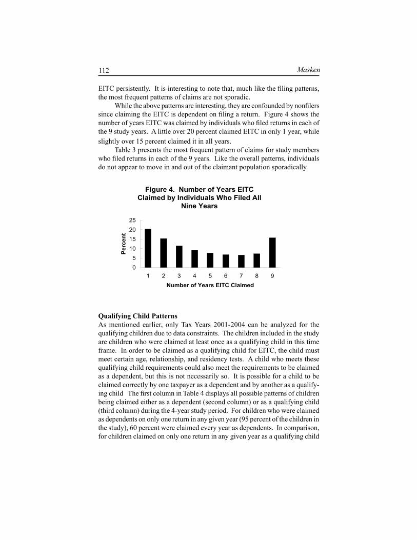
Masken112
EITC persistently. It is interesting to note that, much like the filing patterns, the most frequent patterns of claims are not sporadic.
While the above patterns are interesting, they are confounded by nonfilers since claiming the EITC is dependent on filing a return. Figure 4 shows the number of years EITC was claimed by individuals who filed returns in each of the 9 study years. A little over 20 percent claimed EITC in only 1 year, while slightly over 15 percent claimed it in all years.
Table 3 presents the most frequent pattern of claims for study members who filed returns in each of the 9 years. Like the overall patterns, individuals do not appear to move in and out of the claimant population sporadically.
Qualifying Child PatternsAs mentioned earlier, only Tax Years 2001-2004 can be analyzed for the qualifying children due to data constraints. The children included in the study are children who were claimed at least once as a qualifying child in this time frame. In order to be claimed as a qualifying child for EITC, the child must meet certain age, relationship, and residency tests. A child who meets these qualifying child requirements could also meet the requirements to be claimed as a dependent, but this is not necessarily so. It is possible for a child to be claimed correctly by one taxpayer as a dependent and by another as a qualify-ing child The first column in Table 4 displays all possible patterns of children being claimed either as a dependent (second column) or as a qualifying child (third column) during the 4-year study period. For children who were claimed as dependents on only one return in any given year (95 percent of the children in the study), 60 percent were claimed every year as dependents. In comparison, for children claimed on only one return in any given year as a qualifying child
Figure 4. Number of Years EITC Claimed by Individuals Who Filed All
Nine Years
0510152025
1 2 3 4 5 6 7 8 9Number of Years EITC Claimed
Perc
ent

Longitudinal Study of EITC Claimants 113
(98 percent of children in the study), 31 percent were claimed every year as a qualifying child. Interestingly, about one-half of 1 percent were never claimed as dependents but were claimed as qualifying children for EITC.
Of those being claimed as qualifying children in each of the 4 years, 75 percent were consistently claimed as both a dependent and as a qualifying child by the same primary taxpayer in each year. However, a large number (21 percent), were claimed as both a dependent and qualifying child in each year, but not by the same taxpayer across years. Table 5 illustrates the number and pattern of taxpayers claiming the child as a qualifying child across the years. Each number in the pattern column represents a different taxpayer. For example, the pattern ‘1 2 1 2’ indicates two different taxpayers claiming the child in alternating years, whereas the pattern ‘1 2 3 4’ indicates the child was claimed by a different taxpayer every year.
Next Steps While this analysis provides valuable insight into what taxpayers do, the primary goal of conducting a longitudinal study is to try and understand why taxpayers move in and out of the EITC claimant population. Future research will try to understand from the administrative data why taxpayers enter and why they leave the claimant population. It is also hoped that more retrospective years can be obtained for the children in order to better understand the patterns that exist. It is also of interest to try to understand why some children are claimed by more than one taxpayer, particularly in one given year.

Masken114
Table 1. Most Frequent Filing Patterns
PercentCumulative
PercentX X X X X X X X X 47% 47%- X X X X X X X X 4% 51%X X X X X X X X - 3% 54%X X X - X X X X X 3% 56%- - X X X X X X X 2% 59%- - - X X X X X X 2% 61%- - - - X X X X X 2% 63%X X X X X X X - - 2% 65%- - - - - X X X X 2% 66%X X X X X X - - - 1% 67%- - - - - - X X X 1% 69%X X X X X - - - - 1% 70%X X X - - - - - - 1% 71%X - - - - - - - - 1% 72%- - - - - - - X X 1% 73%X X - - - - - - - 1% 74%X X X X - - - - - 1% 75%
Filing Pattern

Longitudinal Study of EITC Claimants 115
Table 2. Most Frequent Patterns of Claiming EITC
PercentCumulative
PercentX X X X X X X X X 7% 7%X - - - - - - - - 6% 13%- - - - - - - X X 3% 17%- - - - - - - X - 3% 20%X X - - - - - - - 3% 24%- - - - - - X - - 3% 27%- X - - - - - - - 3% 29%- - - - - - X X X 3% 32%- - X - - - - - - 2% 35%X X X - - - - - - 2% 37%- - - - - X - - - 2% 39%- - - - - X X X X 2% 41%- - - - X - - - - 2% 43%- - - X - - - - - 2% 45%- - - - X X X X X 2% 46%X X X X - - - - - 2% 48%- X X X X X X X X 2% 49%- - - - - - X X - 1% 51%
Claims Pattern

Masken116
PercentCumulativePercent
X X X X X X X X X 16% 16%X - - - - - - - - 7% 22%X X - - - - - - - 4% 26%- - - - - - - X - 3% 29%- X - - - - - - - 3% 31%X X X - - - - - - 3% 34%- - - - - - - X X 2% 37%- - - - - - X - - 2% 39%- - - - - - X X X 2% 41%X X X X - - - - - 2% 43%- - X - - - - - - 2% 45%X X X X X X X X - 2% 47%- X X X X X X X X 2% 48%- - - X - - - - - 1% 50%X X X X X - - - - 1% 51%
Claims Pattern
Table 3. Most Frequent Patterns of Claiming EITCby Individuals Who Filed all Nine Years

Longitudinal Study of EITC Claimants 117
Table 4. Pattern of Children Claimed as:
Dependent Qualifying ChildX X X X 60% 31%- X X X 6% 8%- - X X 5% 8%X X X - 5% 7%- - - X 5% 10%X X - - 3% 6%X - - - 3% 8%X X - X 2% 2%X - X X 1% 2%- - X - 1% 4%- X X - 1% 3%- X - - 1% 5%X - - X 1% 1%- - - - 1% n.a.- X - X * 1%X - X - * 1%
* Less than 0.5%
ClaimPattern

Masken118
Table 5. Pattern of Who Claimed the Child for EITC
Percent Cumulative Percent1 1 1 1 77% 77%1 2 2 2 6% 83%1 1 1 2 5% 88%1 1 2 2 4% 92%1 1 2 1 1% 93%1 2 1 1 1% 95%1 1 2 3 1% 96%1 2 3 3 1% 97%1 2 2 3 1% 98%1 2 3 4 1% 99%1 2 2 1 1% 99%1 2 1 2 * 99%1 2 1 3 * 100%1 2 3 1 * 100%1 2 3 2 * 100%
* Less than 0.5%
Pattern
3
Uses of Tax Data
Foertsch u RectorO’HaraD

Changes in tax policy can influence economic incentives for households to work and save and for businesses to invest. Subsequent changes in employment, investment, and incomes can affect Federal tax revenues.
Dynamic analyses capturing such interactions between taxes and the economy are facilitated by integrating macroeconomic models of the economy and microsimulation models of taxation. An important part of that integration is calibrating both models to the same “baseline” forecast.
In this paper, we describe a process for calibrating a macroeconomic model of the U.S. economy and a microsimulation model of the Federal indi-vidual income tax to the Congressional Budget Office’s (CBO’s) January 2006 baseline projections. The microsimulation model is based on the Public-Use Tax File produced by the Statistics of Income (SOI) Division of the Internal Revenue Service (IRS). The macroeconomic model, Global Insight’s U.S. Macroeconomic Model, is based on Bureau of Economic Analysis (BEA) na-tional income and product accounts (NIPA) data.1 Once calibrated to the same official baseline, the two models can be used jointly to simulate the economic and budgetary effects of changes in tax policies. Direct comparisons can then be made between dynamic estimates from the macroeconomic model and conventional estimates from the microsimulation model.
The Congressional Budget Office (CBO) produces biannual baseline projections of the U.S. economy and the Federal budget (generally in January and August of each year). Those projections embody the rules and conven-tions governing a current-services Federal budget. They project gross domestic product (GDP), prices, personal and corporate incomes, and Federal receipts, expenditures, and net saving, among other economic and budgetary variables over 10 years assuming current-law tax (and nontax) policies and the continu-ation of current levels of spending.
CBO’s 10-year baseline projections serve as Congress’s official start-ing point for gauging the budgetary effects of proposed changes in taxes and spending. For example, the Joint Committee on Taxation (JCT) estimates the conventional revenue effects of tax proposals using CBO’s economic and
Calibrating Macroeconomic and Microsimulation Models to CBO’s
Baseline ProjectionsTracy L. Foertsch and Ralph A. Rector,
The Heritage Foundation

Foertsch and Rector 122
budgetary projections as a baseline. JCT’s conventional revenue estimates may include some microeconomic behavioral effects of a change in tax policy. Thus, they may take into account shifts in the timing of transactions and income recognition.2 But they generally exclude the economywide macroeconomic effects of changes in tax policy on Federal receipts. Similarly, CBO uses its own economic and budgetary projections as a baseline when generating con-ventional estimates of the budgetary effects of spending proposals.
Simulation models meant to generate comparable “dynamic” estimates of the economic and budgetary effects of Federal tax and spending proposals should also be calibrated to CBO’s baseline projections. Dynamic estimates include the effects of changes in labor force participation, investment, and interest rates on Federal tax policies. They can differ, sometimes significantly, from conventional revenue estimates. Dynamic estimates that are not made relative to the CBO baseline can provide a broad-brush analysis of a proposed tax policy’s economic and budgetary effects. But they cannot be used as a dynamic alternative to a conventional estimate of the proposed policy’s effects. At best, they can serve as a vehicle for ranking the relative strengths and weak-nesses of alternative proposals.3
We calibrate two models to CBO’s baseline economic and budgetary projections. We typically use both models to evaluate proposed changes in tax policy. The first model is the Global Insight (GI) short-term U.S. Macroeco-nomic Model. The second is a proprietary microsimulation model of individual income tax returns developed by analysts at The Heritage Foundation’s Center for Data Analysis.
A CBO-like baseline forecast is constructed using the Global Insight model and the details that CBO provides about its economic and budgetary projections. Using the GI model, we infer the implications of CBO’s current-law assumptions for key macroeconomic variables, including personal consumption, investment, employment, and the components of NIPA personal income. In combination with SOI data, the microsimulation model uses the final CBO-like baseline forecast and estimated relationships between NIPA personal income and personal income reported to the IRS to project the characteristics of individual income tax records. The result is an integrated calibration of macroeconomic and microsimulation models that can be used for policy simulations.
The paper proceeds as follows. The second section gives key facts about CBO’s baseline economic and budgetary projections. We focus on CBO’s current-law assumptions and the variables CBO publishes, and we use, in calibrating to CBO’s baseline projections. The third section discusses our general approach to calibrating the GI and microsimulation models to CBO’s published projections. The fourth section concludes by examining the impli-

Calibrating Macroeconomic and Microsimulation Models 123
cations of using the calibrated macroeconomic and microsimulation models for tax policy analysis.
An Overview of CBO’s Baseline ProjectionsCBO’s biannual baseline projections play a dual policy role. They inform policymakers about the implications of current fiscal policies for Federal budgetary aggregates, and they provide a common baseline for scoring the budgetary effects of proposed changes in taxes and spending. As a result, CBO’s economic and budgetary projections are unique when compared with other--particularly commercial--forecasts. Specifically, they embody current law, and they explicitly assess the impact of current-law policies (fiscal and nonfiscal) on key indicators of economic activity.
CBO’s Current-Policy Assumptions. A set of detailed rules govern the pro-cess by which CBO’s economic and budgetary projections embody current law and policy. The Balanced Budget and Emergency Deficit Control Act of 1985 and various other conventions for a Federal baseline require CBO to produce a very specific kind of forecast.4 CBO’s baseline budgetary projections--and, hence, the CBO-like forecast we construct to replicate them--cannot anticipate changes in current law. Rather, they must assume that future taxes, spend-ing, and other (nonfiscal) policy measures evolve as stipulated by previously enacted legislation.
This means that CBO’s 10-year revenue projections assume no change in tax provisions or tax rates unless such a change is already included in current law. Thus, CBO’s January 2006 baseline revenue projections assume the 2008 expiration (or “sunset”) of the preferential capital gain and dividend tax rates enacted under the Jobs and Growth Tax Relief Reconciliation Act (JGTRRA)5 and the 2010 expiration of tax relief provisions enacted under the Economic Growth and Tax Relief Reconciliation Act (EGTRRA).6 Similarly, despite widespread discussion of the issue, CBO’s revenue projections do not include any changes to the alternative minimum tax (AMT). Private sector forecasts typically anticipate some change in the current law governing the AMT--if only because without some adjustment, a growing number of taxpayers will see their tax burdens increase as a result of the AMT.
CBO’s budgetary projections also exclude changes in Federal spending not already set by current policies. Thus, CBO uses current-law eligibility and benefits criteria to project mandatory spending on entitlement programs like Social Security, Medicare, and Medicaid over the 10-year budget period.7 Current law in the form of appropriations bills does not dictate a path for discretionary spending and supplemental budget authority beyond the current

Foertsch and Rector 124
budget year.8 However, the Balanced Budget and Emergency Deficit Control Act of 1985 requires that CBO assume that both discretionary spending and supplemental appropriations in the most recent year’s budget authority continue in each subsequent year of CBO’s 10-year budgetary baseline.9 In that baseline, projected current-services outlays keep pace with projected current-services budget authority. Both projected budget authority and outlays rise because CBO adjusts budget authority to offset projected inflation and cost-of-living adjustments.
CBO assesses the impact of GDP, prices, interest rates, incomes, and other economic variables on current-law revenues and spending over a 10-year period. CBO’s baseline economic projections consist of two conceptually and analytically distinct components--a 2-year (short-term) forecast of cyclical fluctuations and a separate 8-year (medium-term) projection of potential output (GDP).10 This split in the budget period determines how CBO assesses the economic implications of current-law fiscal policies.
In the short term, CBO allows the path of GDP to deviate from that of its underlying potential.11 CBO gauges the impact of the gap between actual and potential GDP on a range of economic variables. Those variables include inflation, interest rates, employment, personal and corporate incomes, personal consumption and saving, and residential and business fixed investment. CBO also anticipates how monetary policy, exchange rates, and energy prices as well as recently enacted changes in current-law policies (fiscal and nonfiscal) are likely to affect fluctuations in aggregate demand. For example, the August update to CBO’s January 2003 The Budget and Economic Outlook estimated the impact of JGTRRA’s partial-expensing provisions on business fixed investment in 2003 and 2004.12 It also discussed the effects of JGTRRA’s accelerated tax cuts on personal saving.13
In the medium term, CBO does not project fluctuations in aggregate de-mand. Instead, it uses a growth model to estimate potential GDP and assumes that any gap between actual GDP and estimated potential GDP remaining at the end of the short-term forecast closes over the subsequent 8 years.14 Other key economic variables are similarly assumed to trend toward an estimated long-run average over the medium term. For example, CBO’s projected rate of return on 10-year Treasury notes equals 5.2 percent from 2007, 1-year prior to the start of CBO’s medium-term projections.15 CBO’s projected unemployment rate attains its long-run natural rate (5.2 percent) only 2 years later, in 2009. In contrast, the unemployment rate in Global Insight’s February 2006 short-term U.S. Macroeconomic forecast fluctuates around its long-run natural rate over much of GI’s 10-year forecast horizon.16
As a result, CBO’s medium-term projections are largely limited to as-sessing the impacts of current-law fiscal policies on potential GDP and related

Calibrating Macroeconomic and Microsimulation Models 125
variables, notably potential labor hours and capital. For example, EGTRRA’s expiring provisions and increasing taxpayer exposure to the AMT are likely to generate a steady rise in average marginal tax rates on wages. CBO ad-justs potential labor hours for the anticipated disincentive effects, layering an estimated decline in the supply of labor hours onto a baseline projection that reflects long-run trends in demographics and labor force participation.17 CBO also estimates the potential effects of rising Federal deficits and debt on the capital stock. It includes some “crowding out” of private investment into its growth model, using projections of net foreign investment to gauge the extent to which increased capital inflows from abroad are likely to offset declines in national saving and domestic private investment.18
Federal Policy Assumptions Found in Other Macroeconomic Forecasts. Unlike CBO, other forecasters--particularly commercial forecasters--are not restricted by the rules and conventions governing a Federal baseline. They can therefore build into their forecasts expected changes in taxes and spending that are inconsistent with a current-law baseline. They can also anticipate changes in other, nonfiscal current-law policies. Those expectations about future fiscal and nonfiscal policies can dramatically impact projected values of key economic and budgetary aggregates.
For example, GI’s February 2006 U.S. Macroeconomic forecast assumes a partial extension of expiring tax relief provisions originally enacted under EGTRRA and JGTRRA. As a result, GI projects a far more gradual increase than does CBO in NIPA personal income tax revenues as a share of GDP (see Figure 1A). Unsurprisingly, GI also projects higher levels of NIPA personal dis-posable income as a share of GDP--particularly after 2010 (see Figure 1B).
Commercial forecasts can also include expected changes in Federal spending that are inconsistent with a current-services budget.19 Both CBO’s baseline budgetary projections and GI’s February 2006 U.S. Macroeconomic forecast allow for growth in Federal defense spending over the next 10 years. However, GI consistently projects higher levels of defense spending as a share of GDP (see Figure 2).
Initial differences between CBO’s and GI’s projections of defense spend-ing seem in part explained by different assumptions about the rate of spending. Federal defense spending fell in the fourth quarter of 2005, after expanding at a double-digit rate in the third quarter of the same year.20 It followed a similar pattern in the final two quarters of 2004 before bouncing back strongly in the first quarter of 2005. GI largely attributes both third-to-fourth quarter declines to delays in the passage of the current fiscal years’ defense appropriations bill.21 Using history as a guide, it assumes a strong rebound in defense spending in
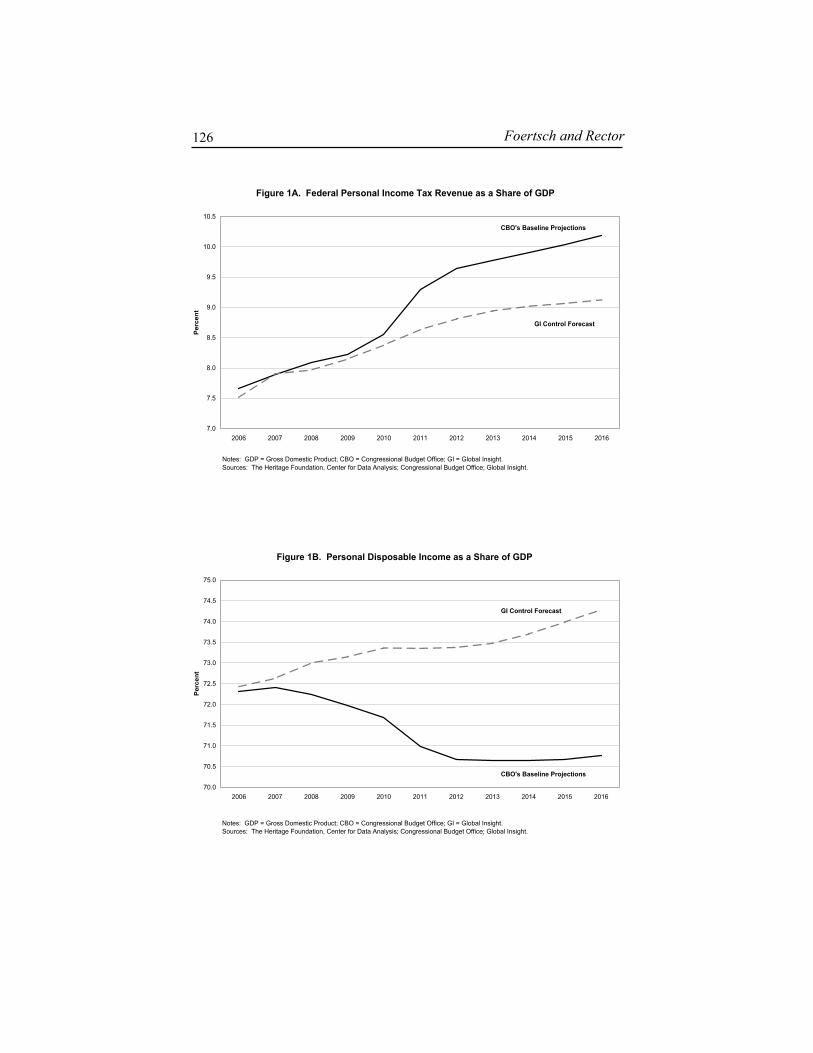
Foertsch and Rector 126
Figure 1B. Personal Disposable Income as a Share of GDP
70.0
70.5
71.0
71.5
72.0
72.5
73.0
73.5
74.0
74.5
75.0
2006 2007 2008 2009 2010 2011 2012 2013 2014 2015 2016
Perc
ent
Notes: GDP = Gross Domestic Product; CBO = Congressional Budget Office; GI = Global Insight.Sources: The Heritage Foundation, Center for Data Analysis; Congressional Budget Office; Global Insight.
CBO's Baseline Projections
GI Control Forecast
Figure 1A. Federal Personal Income Tax Revenue as a Share of GDP
7.0
7.5
8.0
8.5
9.0
9.5
10.0
10.5
2006 2007 2008 2009 2010 2011 2012 2013 2014 2015 2016
Perc
ent
Notes: GDP = Gross Domestic Product; CBO = Congressional Budget Office; GI = Global Insight.Sources: The Heritage Foundation, Center for Data Analysis; Congressional Budget Office; Global Insight.
CBO's Baseline Projections
GI Control Forecast

Calibrating Macroeconomic and Microsimulation Models 127
the first half of 2006. Such a strong rebound in Federal defense spending is not as apparent in CBO’s budgetary projections.22
After 2006, CBO projects current fiscal-year defense spending forward at the rate of inflation. GI is not restricted by such current-services budget requirements. Thus, through 2010, GI’s standard forecast includes additional supplemental appropriations for Iraq and Afghanistan. From 2011 to 2016, it includes a slightly higher deflator for military wages and salaries. The result is a persistent gap between CBO and GI projections of NIPA Federal defense spending.23
Finally, commercial forecasts can anticipate changes in other (nonfiscal) current-law policies. The Pension Funding Equity Act of 2004 (PFEA) expired at the end of 2005. PFEA temporarily lowered firms’ required contributions to defined-benefit (DB) pension plans. It did so by setting the maximum appli-cable discount rate used to calculate the present value of DB pension liabilities above the rate required by the Employment Retirement Income Security Act of 1974 (ERISA). In general, the higher the applicable discount rate, the lower the present value of pension liabilities and the lower required DB pension contributions.24
GI’s February 2006 U.S. Macroeconomic forecast assumes a change in current law that extends PFEA’s higher discounting through 2006. CBO’s baseline economic and budgetary projections do not.25 As a result, GI makes
Figure 2. Federal Defense Spending as a Share of GDP
3.4
3.6
3.8
4.0
4.2
4.4
4.6
4.8
2006 2007 2008 2009 2010 2011 2012 2013 2014 2015 2016
Per
cent
Notes: GDP = Gross Domestic Product; CBO = Congressional Budget Office; GI = Global Insight.Sources: The Heritage Foundation, Center for Data Analysis; Congressional Budget Office; Global Insight.
CBO's Baseline Projections
GI Control Forecast

Foertsch and Rector 128
no specific adjustments to corporate (book) profits or to the corporate income tax base to reflect a jump in DB contributions. CBO includes such adjustments, dramatically lowering projected corporate profits as a share of GDP relative to the GI forecast (see Figure 3).
Limitations of Using CBO’s Published Baseline Projections. We calibrate a commercial macroeconomic model of the U.S. economy and a proprietary microsimulation model of individual income tax returns to CBO’s baseline pro-jections. The challenges faced in calibrating the two models differ. However, for both models, a common factor complicates our work. CBO publishes only a small subset of the economic and budgetary variables making up its baseline projections (see Table 1). This limits the number of variables available as guides in adjusting the two models to reflect CBO’s current-law assumptions.
Calibrating the Global Insight Model. We develop our CBO-like baseline forecast using GI’s February 2006 U.S. Macroeconomic forecast as a starting point (or control).26 GI’s U.S. Macroeconomic forecasts typically include ex-pected changes in fiscal and nonfiscal policies. The calibration procedure in part involves iteratively adjusting the control forecast to remove the effects of those expectations so that our CBO-like forecast is consistent with current law.
Figure 3. Corporate Profits as a Share of GDP
9.0
9.5
10.0
10.5
11.0
11.5
12.0
12.5
2005 2006 2007
Perc
ent
Notes: GDP = Gross Domestic Product; CBO = Congressional Budget Office; GI = Global Insight.Sources: The Heritage Foundation, Center for Data Analysis; Congressional Budget Office; Global Insight.
CBO's Baseline Projections
GI Control Forecast

Calibrating Macroeconomic and Microsimulation Models 129
Adjusting the control forecast to match CBO’s baseline budgetary projec-tions is relatively straightforward. CBO publishes all but a handful of needed NIPA Federal revenue and spending projections. It also provides a detailed crosswalk between its NIPA Federal budget numbers and its projections of unified (budget) Federal revenues and unified Federal outlays.27
However, CBO does not publish its projections of a number of key mac-roeconomic and income variables. Those variables include the components of GDP, NIPA taxable personal income (with the exception of wage and salary income), and national saving (with the exception of NIPA net Federal govern-ment saving).28 They also include a number of miscellaneous items describing critical assumptions (policy and otherwise) underlying CBO’s 2-year forecast and medium-term projections.
For example, CBO does not typically describe in great detail its projec-tions of the trade-weighted U.S. dollar exchange rate, the price of oil, and the Federal funds rate. Rather, the economic outlook chapter of The Budget and Economic Outlook indicates CBO’s expectations for their levels or movements in the short term.29 When calibrating the GI model to CBO’s baseline economic projections, we use such statements as guides in adjusting (if necessary) GI’s projections of equivalent variables.
Thus, in August 2005, CBO indicated that it expected oil prices to stop rising--but not to “retreat” to pre-2004 levels--during 2005 and 2006.30 In January 2006, CBO again indicated that it expected oil prices to stabilize in 2006.31 We adjusted a weighted average price of imported crude in the GI model appropriately. Similarly, in August 2005, CBO anticipated that the Federal Reserve would continue to raise the target for the Federal funds rate until it reached a neutral rate. CBO observed that the consensus of financial market participants was consistent with a neutral rate ranging between 4 percent and 5 percent.32 In January 2006, CBO reconfirmed its outlook for monetary policy, specifying that the consensus of financial market participants put the expected Federal funds target rate at 4.75 percent by mid-2006.33
More significantly, CBO does not typically provide sufficient detail to establish how it adjusts a number of key macroeconomic and income vari-ables to reflect current law. Figures 4 and 5 reorganize NIPA data as a series of income and expenditure flows among institutional sectors of the economy (households, firms, government, rest of the world, etc.).34 Moving across the columns gives an accounting of income flows among the sectors. Moving down the rows gives an accounting of expenditure flows.
Figure 4 broadly summarizes the level of detail we require for calibration of the microsimulation model and for policy analysis. For example, calibrat-ing the microsimulation model to CBO’s baseline budgetary projections of individual income tax receipts requires projections of the individual compo-

Foertsch and Rector 130
Figure 4. National Income and Product Accounts (NIPA) Income-and-Expenditure Flows(1) (2) (3) (4) (5) (6) (7) (8) (9) (10)
Production (1) Domestic Output
Goods and Services (2)
PersonalConsumption
FederalConsumption and Gross Investment
State & Local Consumption and Gross Investment
Private Domestic Investment Exports
LaborIncome (3)
Compensation of Employees
CapitalIncome (4)
Operating Surplus
Households (5)Wage and Salary Income, Other Labor Income
ProprietorIncome, Rental
Income, Net Interest Income
TransferPayments from
Business,Dividend Income
Federal Transfer Payments, Net
Interest Payments
State & Local Transfer
Payments, Net Interest Payments
Enterprises (6)
Corporate Profits, Transfer
Payments by Business
FederalGovernment (7)
Federal Taxes on Production and
Imports (Less Net Subsidies,
Customs Duties, and Excise Taxes)
Federal Customs Duties and Excise
Taxes
Federal Social Insurance Tax
Receipts
Federal Personal Tax Payments,
Transfer Receipts from Persons
Federal Corporate Income Tax Payments,
Transfer Receipts from Business
Federal Tax Receipts from
ROW
State & Local Government (8)
State & Local Taxes on
Production and Imports (Less Net
Subsidies and Sales Taxes)
State & Local Sales Taxes
State & Local Social Insurance
Tax Receipts
State & Local Personal Tax
Payments,Transfer Receipts
from Persons
State & Local Corporate Income
Tax Payments, Transfer Receipts
from Business
Federal Grants-in-Aid to State and
LocalGovernments
Gross Capital Formation (9)
Consumption of Fixed Capital Personal Saving Retained
EarningsNet Federal
SavingNet State & Local
SavingNet Foreign Investment
Rest of World (10)
ImportsNet Factor
Payments to ROW
Net Transfer Payments to
ROW
Corporate Taxes Paid to ROW,
TransferPayments to
ROW
Social Insurance Payments, Other
Transfers to ROW
Notes: ROW = rest of the world.
Private domestic investment includes both private domestic fixed investment and changes in inventories.
Net factor payments to the ROW equal the difference between factor service imports and exports of factor services.
Source: The Heritage Foundation, Center for Data Analysis.
Net interest income equals personal interest income minus the sum of interest payments by individuals and net interest payments by government (federal and state and local).
Operating surplus is a balancing item equal to the difference between value added and the sum of compensation of employees and taxes on production and imports (less net subsidies). It measures the “…surplus or deficit accruing from processes of production before deducting any explicit or implicit interest charges, rents, or other property income payable on financial assets, land, or tangible non-produced assets required to carry on the production." For unincorporated enterprises owned by households, this component of value added is called mixed income. See paragraph 7.82, at http://unstats.un.org/unsd/sna1993/tocLev8.asp?L1=7&L2=5 (July 19, 2006).
Net operating surplus excludes consumption of fixed capital.
Corporate profits here refer to before-tax economic profits. The Congressional Budget Office (CBO) publishes projections of before-tax book profits.
nents of NIPA personal income.35 Calculating the Federal corporate income tax requires projections of both corporate profits and the corporate income tax base. Finally, doing dynamic analyses of fiscal policy requires the ability to quantify the effect of changes in taxes and spending on the components of GDP and personal income.
The Global Insight model, once calibrated to CBO’s published baseline projections, provides this level of detail. A forecasting model like Global In-sight provides unique advantages to analysts constructing a CBO-like baseline forecast. This is because it includes enough structural detail to fill in the blanks

Calibrating Macroeconomic and Microsimulation Models 131
left by CBO. Figure 5 highlights the extent of those blanks. It shows the same reorganization of NIPA income and expenditure flows as Figure 4, but with identifiers only in the cells for which CBO publishes its baseline economic projections. We use the GI model to help us infer consistent approximations of CBO’s projections of the missing income and expenditure flows.
Although useful for policy evaluation purposes, CBO’s current-law assumptions complicate our efforts to infer those projections using the GI model. For example, the control forecast implicitly assumes some extension of EGTRRA’s expiring provisions after 2010. It therefore includes levels of personal consumption and saving that are higher than those projected by CBO. The calibration procedure involves iteratively lowering the projected rate of growth in personal consumption implied by the control forecast so that the projected personal saving rate is not unreasonable. Unfortunately, CBO typically provides little or no detail on how it adjusts consumption and saving
Figure 5. NIPA Income-and-Expenditure Flows For Which Projections Are Available from CBO(1) (2) (3) (4) (5) (6) (7) (8) (9) (10)
Production (1)
Goods and Services (2)
FederalConsumption and Gross Investment
LaborIncome (3)
CapitalIncome (4)
Households (5)Wage and Salary
Income
Federal Transfer Payments, Net
Interest Payments
Enterprises (6) Corporate Profits
FederalGovernment (7)
Federal Taxes on Production and
Imports (Less Net Subsidies)
Federal Social Insurance Tax
Receipts
Federal Personal Tax Payments,
Transfer Receipts from Persons
Federal Corporate Income Tax Payments,
Transfer Receipts from Business
Federal Tax Receipts from
ROW
State & Local Government (8)
Federal Grants-in-Aid to State and
LocalGovernments
Gross Capital Formation (9)
Net Federal Saving
Rest of World (10)
Notes: NIPA = national income and product accounts; CBO = Congressional Budget Office.
See notes to Figure 4.
Corporate profits here refer to before-tax economic profits. CBO publishes projections of before-tax book profits.
Source: The Heritage Foundation, Center for Data Analysis.

Foertsch and Rector 132
to reflect EGTRRA’s sunset. As a result, we have only personal judgment and historical data to rely upon when determining an appropriate current-law level for the personal saving rate.
Similarly, CBO typically publishes only its projections of NIPA taxable personal income and wage and salary income.36 Calibration requires allocat-ing the difference between the two among personal dividend income, personal interest income, personal rental income, and proprietors’ income (farm and nonfarm). We can use information from the control forecast to do this. How-ever, the control forecast implicitly assumes some extension of JGTRRA’s preferential tax rates on dividend income. And CBO typically provides little or no additional detail to use in deriving an allocation that would be more consistent with current-law assumptions.
Calibrating the Microsimulation Model. The primary challenge we face in calibrating the microsimulation model to CBO’s baseline projections is a bit different. The inputs into the calibration procedure for the microsimulation model already reflect current law. For example, we use a number of economic variables from the CBO-like forecast. We also use many of the Federal revenue projections published in the revenue outlook chapter of CBO’s The Budget and Economic Outlook.
However, economic inputs from the CBO-like forecast provide only a starting point. This is because they are expressed as NIPA values and not as amounts reported on tax returns. The microsimulation model simulates the effects of tax law changes on a representative sample of over 100,000 Federal individual income tax returns based on the characteristics of the individuals and families associated with those returns. A crosswalk is therefore needed to reconcile the definitional and timing differences among NIPA personal income, the amount of income reported on income tax returns, and supplementary information obtained from the Current Population Survey (CPS). Non-NIPA components of individual income such as capital gains, pensions, annuities, and individual retirement accounts must also be added. Data for tax return filers and nonfilers must then be extrapolated (“aged”) over the 10-year budget period.
As a result, a key part of our calibration procedure involves deriving de-tailed targets for the amount of tax-related income, the distribution of tax-related income, and the demographic characteristics of the U.S. population. These targets are then used to adjust data on records in the microsimulation model so that those records are in aggregate consistent with CBO’s baseline economic and budgetary projections. Such information is not typically published by CBO and cannot generally be obtained directly from CBO or other sources. The exceptions are demographic projections, which are available from the Census

Calibrating Macroeconomic and Microsimulation Models 133
Bureau, and projections of total individual capital gain realizations, which CBO publishes every January in The Budget and Economic Outlook.37
Calibrating Macroeconomic and Microsimulation Models to CBO’s Baseline ProjectionsCalibration to CBO’s baseline projections begins with the macroeconomic model. We first calibrate the Global Insight model to CBO’s published economic projections and NIPA Federal revenue and spending projections. We refer to output from the calibrated GI model as the final CBO-like forecast. The final CBO-like baseline forecast not only replicates the published details of CBO’s current-law baseline but also includes projections of key macroeconomic and income variables excluded from them.38
We then calibrate the microsimulation model to CBO’s baseline projec-tions. In doing so, we use data from the SOI and the Census Bureau as well as economic variables from the final CBO-like forecast. Those economic vari-ables include nominal GDP, corporate profits, the consumer price index (CPI) for all urban consumers, the components of NIPA taxable personal income, NIPA transfer payments to persons (Federal as well as State and local), and NIPA State and local tax revenues. The calibrated microsimulation model that results approximates CBO’s baseline projections of key economic and income variables and individual income tax revenues.
Calibrating the Global Insight Macroeconomic Model. Calibrating the Global Insight model to CBO’s current-law baseline involves iteratively adjusting the control forecast so that, when solved, the Global Insight model endogenously reproduces all projections of economic and budgetary variables published by CBO.39 This is a multistep process. In each step, we replace variables in the GI model with CBO’s projections. We then solve the GI model so that those variables that have not been targeted adjust. In essence, we are using econometrically estimated relationships and accounting identities within the GI model to create a forecast that is consistent with what we know about CBO’s baseline economic and budgetary projections.
Step 1. We first set key economic assumptions and price levels. This process involves setting the price of oil and the trade-weighted U.S. dollar exchange rate so that they are consistent with what we know about CBO’s baseline eco-nomic assumptions. It also involves setting some policy variables such as the statutory corporate income tax rate and the Federal social insurance tax rate so that they are consistent with CBO’s baseline revenue projections. Finally, it

Foertsch and Rector 134
requires that we impose CBO’s projections of certain key economic variables. Those variables include the unemployment rate, the 3-month Treasury bill rate, and the 10-year Treasury note rate.
The 3-month Treasury bill rate is also used to set the Federal funds rate. The GI control forecast includes a projection of the Federal funds rate that differs from what CBO describes as the consensus of financial market participants. We correct for this by imposing a target for the Federal funds rate that is broadly consistent with not only CBO’s description of financial market consensus but also CBO’s projection of the 3-month Treasury bill rate. We obtain this target by first calculating the spread in the control forecast between the 3-month Treasury bill rate and the Federal funds rate. We then apply this spread, with some adjustments, to CBO’s projection of the 3-month Treasury bill rate.
We complete the first step by setting price levels for all components of GDP. CBO publishes 10-year projections of year-over-year percentage changes in an aggregate GDP price index. We use this along with information about the components of the GDP price deflator contained in the GI control forecast to set all underlying GDP price indices so that they are consistent with CBO’s projection of GDP inflation.
Setting price levels early in the calibration procedure is critical. This is because many exogenous Federal outlays variables in the Global Insight model are in real (inflation-adjusted) terms. We therefore require a price level variable to convert CBO’s nominal baseline budgetary projections for those variables into consistent real targets.
Step 2. In the second step, we set Federal spending (outlays) net of Federal interest payments.40 Federal spending broadly includes Federal consumption spending, Federal transfer payments, and other spending items in the Federal Government’s budget.
CBO publishes its projections for most--but not all--of the Global In-sight model’s NIPA federal spending variables. For example, the Federal Government’s budget includes Federal social benefits to the rest of the world and Federal subsidies. CBO publishes its projections of both aggregates. We replace GI’s projections of these variables with CBO’s published NIPA pro-jections. Similarly, CBO publishes its projection of Federal net investment.41 We combine this with CBO’s baseline projections of NIPA defense and non-defense consumption of fixed capital to obtain a NIPA target for Federal gross investment.
However, CBO does not provide baseline projections for all NIPA Federal spending variables. In some instances, we rely on the GI control forecast to obtain needed targets. For example, Federal consumption spending includes both defense and nondefense “other” purchases of goods and services and wages

Calibrating Macroeconomic and Microsimulation Models 135
and salaries for personnel. CBO only publishes its projection of the sum of the two (labeled defense and nondefense “consumption”). In the absence of any additional information from CBO, we set “other” Federal purchases of goods and services equal to the difference between CBO’s projections of defense and nondefense “consumption” and GI’s projections of defense and nondefense outlays for personnel
In other instances, we derive needed targets from CBO’s published pro-jections of budget (unified) Federal outlays. Federal transfer payments include both social benefits to persons and grants-in-aid to State and local governments. CBO publishes its NIPA projection of grants-in-aid to State and local govern-ments. However, it publishes only budget projections of Federal spending on Social Security, Medicare, and Medicaid. To obtain equivalent NIPA targets, we use historical Government social benefits data from CBO and BEA to ad-just CBO’s published projections of Social Security, Medicare, and Medicaid spending for administrative costs.42
Step 3. In the third step, we adjust the components of GDP so that they are consistent with not only CBO’s projections of real GDP and real Federal spend-ing (on both current consumption and investment) but also current laws and policies. We follow a three-step procedure.
First, we adjust all components of GDP for which CBO’s baseline pro-jections are unavailable. Those components include personal consumption, gross private domestic investment, State and local government purchases of goods and services (including State and local investment), and net exports. We scale all four aggregates proportionately so that they are consistent with CBO’s projections of real GDP and real Federal spending. We do so using information from the control forecast about the allocation of GDP among its constituent components.
Second, we derive a target for personal consumption that is more in line with CBO’s current-law assumptions. A target for real personal consumption obtained using information strictly from the control forecast is likely to be too high. This is because the control forecast does not assume current law. CBO does not describe in detail its baseline projections of personal consumption. However, the economic outlook chapter of The Budget and Economic Outlook typically gives annual rates of growth in personal consumption for the 2 years covered by CBO’s short-term economic forecast.43 We derive a target for real personal consumption using those growth rates and some judgment about the likely impacts on personal saving of not extending EGTRRA’s and JGTRRA’s expiring provisions after 2010.
Finally, we readjust all components of GDP for which we do not have published projections from CBO. At this stage, those components include gross

Foertsch and Rector 136
private domestic investment, State and local government purchases of goods and services, and net exports. We scale all three aggregates proportionally so that they are jointly consistent with CBO’s projections of real GDP and real Federal spending and our target of real personal consumption. In doing so, we again rely primarily on information from the control forecast.
Before continuing to step 4, we consider State and local government operating surpluses in our CBO-like forecast. At this point in the calibration, State and local government purchases of goods and services, when combined with all other State and local spending, could exceed State and local revenues by a wide margin (or vice versa). CBO does not typically describe in any great detail its baseline projections for State and local government budgets. However, we assume that those budgets are roughly in balance. We adjust components of State and local spending (other than purchases of goods and services) to put State and local budgets as close as possible to a slight surplus position in the final CBO-like baseline forecast.
Step 4. We next adjust potential (full-employment) GDP in the GI model to be consistent with CBO’s medium-term projections of the rates of growth in potential GDP and the potential labor force.44
We use the GI control forecast as a starting point. CBO does not regularly publish levels-estimates of either potential GDP or the potential labor force.45 We therefore adjust the projected levels of both variables in the control forecast to be consistent with CBO’s published growth rate projections. We apply CBO’s projections of the growth rate of the potential labor force directly, adjusting the projected level of the potential labor force in the control forecast. We target the growth rate of potential GDP only indirectly, adjusting among other variables the exogenous trend in total factor productivity in the control forecast.
Step 5. In the fifth step, we adjust the components of NIPA taxable personal income. CBO typically publishes its projections of NIPA taxable personal income only in the January release of The Budget and Economic Outlook.46 CBO’s NIPA taxable personal income includes wage and salary income (both private and government), personal interest income, personal dividend income, personal rental income, and proprietors’ income (farm and nonfarm). CBO publishes projections only of the wage and salary component of NIPA taxable personal income.
We rely primarily on information from the control forecast when deriv-ing targets for the remaining components of NIPA taxable personal income. We follow a two-step procedure. First, we set private wages and salaries by subtracting GI’s projections of defense and nondefense outlays for personnel (government wages and salaries) from CBO’s published projection of NIPA

Calibrating Macroeconomic and Microsimulation Models 137
wage and salary income. Second, we allocate the difference between CBO’s published projections of NIPA taxable personal income and NIPA wage and salary income among the remaining components of NIPA taxable personal income. In doing so, we apply information from the control forecast. To the extent possible, we also adjust any targets we derive for the components of NIPA taxable personal income so that they are more in line with CBO’s cur-rent-law assumptions.
For example, at the time we constructed our January 2006 CBO-like forecast, current law stipulated the 2008 sunset of JGTRRA’s preferential tax rates on dividend income. The control forecast assumed some extension of those preferential rates and, thus, in all likelihood, a different path for personal dividend income than would be included in CBO’s baseline projections. In the past, we have attempted to adjust our target for personal dividend income accordingly. Unfortunately, we could not easily confirm the accuracy of our income target and, therefore, did not attempt to include an equivalent adjust-ment in our January 2006 CBO-like forecast.
Before continuing to step 6, we consider the personal saving rate in our CBO-like forecast. Personal saving is a residual variable in the GI model. This means that CBO’s published projections of NIPA taxable personal income and our target for NIPA personal consumption jointly determine projected personal saving and, thus, the personal saving rate in the final CBO-like forecast.
The calibration procedure can yield what seems like an unrealistically negative personal saving rate if we do not adjust for the likely impact of EGTRRA’s sunset on personal consumption. In the final CBO-like forecast, the personal saving rate averages roughly -0.1 percent between 2007 and 2010 and roughly -1.1 percent between 2011 and 2016. When initially construct-ing the final CBO-like forecast, we did not adjust personal consumption for an increase in personal income tax payments and, hence, a drop in personal disposable income after 2010. As a result, the personal saving rate averaged well above -1.1 percent in absolute value. This compares with a personal sav-ing rate of about -0.5 percent in 2005.47
Step 6. We next adjust the CBO-like forecast to be consistent with CBO’s baseline projections of NIPA Federal tax receipts. NIPA Federal tax receipts include taxes from the rest of the world, taxes on production and imports, taxes on personal income, and taxes on corporate income.48 CBO publishes projec-tions for all four. Setting Federal taxes from the rest of the world and Federal taxes on production and imports is relatively straightforward. We replace GI’s projections with published projections from CBO’s current-law baseline.
Setting Federal taxes on personal and corporate incomes is more involved. This is because doing so requires that we separately target both average ef-

Foertsch and Rector 138
fective Federal income tax rates and the GI model’s Federal personal and corporate income tax bases. For example, the GI model defines the Federal personal income tax base as a function of both NIPA taxable personal income and individual capital gains. CBO publishes projections of individual capital gains realizations.49 We must therefore adjust our target for the Federal personal income tax base to reflect CBO’s projections of capital gains.
The GI model also includes an approximation of the corporate income tax base. The Global Insight model defines the Federal corporate income tax base as before-tax corporate (book) profits minus rest-of-world corporate prof-its and the profits of the Federal Reserve.50 CBO publishes its projections of corporate (book) profits. However, targeting corporate profits is complicated because they are a residual of gross national product (GNP) in the GI model.51
As such, they cannot simply be replaced in our CBO-like forecast with CBO’s published projections.
Rather, we iteratively modify the statistical discrepancy in the CBO-like forecast to target corporate profits indirectly. The statistical discrepancy in the final CBO-like forecast generally exceeds the statistical discrepancy in the control forecast. This is in part because we adjust corporate profits in the CBO-like forecast to fall roughly in line with the jump in contributions to de-fined-benefit pension plans forecast by CBO. Thus, the statistical discrepancy averages just under 0.4 percent of GDP between 2007 and 2016 in the control forecast. It averages just over 0.7 percent of GDP over the same period in the final CBO-like forecast.
Before completing step 6, we calculate average effective Federal tax rates on personal and corporate incomes. These average effective rates reconcile CBO’s projections of Federal personal and corporate income tax revenues with approximations of the Federal personal and corporate income tax bases included in the final CBO-like baseline forecast.52 We impose these average effective tax rates in the CBO-like forecast.
Step 7. In the final step, we complete calibration of the GI model to CBO’s baseline projections. We begin by setting the levels of publicly-held Federal debt and net Federal interest payments in the CBO-like forecast.53
We only indirectly impose CBO’s projection of the stock of publicly-held Federal debt. A net change in publicly-held Federal debt is calculated using CBO’s published projections of unified Federal surpluses along with CBO’s published projections of the Federal Government’s other means of financing publicly-held debt. That net change is used to make quarterly adjustments to the GI model’s variable for publicly-held Federal debt that are consistent with CBO’s other published budgetary projections. After setting the stock of

Calibrating Macroeconomic and Microsimulation Models 139
Federal debt, we impose a target for net Federal interest payments. That target is calculated using CBO’s projections of gross Federal interest payments and Federal income on assets.54
After setting net Federal interest payments, we make our final adjustments to the CBO-like forecast. These final adjustments include setting the level of the consumer price index (CPI) to be consistent with CBO’s projections of CPI inflation. They also include finetuning average effective Federal tax rates on personal and corporate incomes and for Federal contributions to social insurance so that the final CBO-like forecast is consistent with CBO’s published projec-tions of Federal tax receipts. Finally, they include slight adjustments to the statistical discrepancy to ensure that the GI model calibrated to the final CBO-like forecast reproduces CBO’s published projection of corporate profits.
Calibrating the Microsimulation Model. We next calibrate the microsimu-lation model of individual income tax returns to CBO’s baseline projections. Data produced by the SOI play a vital role in helping us develop a database for use in doing tax policy analysis. A base-year SOI sample of individual income tax returns is adjusted so that, when the model simulates current-law tax provi-sions, the results are consistent with CBO’s baseline economic projections and approximate CBO’s individual income tax revenue projections.
The final CBO-like baseline forecast provides a number of NIPA measures of personal and business income that we use in calibration. Those NIPA income measures include wage and salary income, investment income (personal interest and dividend income), proprietors’ income (farm and nonfarm), other busi-ness income (including personal rental income), transfer payments to persons (Federal as well as State and local), and corporate profits. The final CBO-like forecast also provides price-level variables (the CPI for all urban consumers and the GDP deflator for medical goods and services) and some NIPA budget-ary variables (State and local tax revenues) used in calibration.
The Public-Use Tax File. The core data for the microsimulation model are derived from a comprehensive cross-sectional sample of individual income tax returns produced by the SOI. Analysts at the U.S. Department of the Treasury’s Office of Tax Analysis (OTA), JCT, and CBO use the records of individual income tax returns included in that sample to develop revenue estimates and to research tax policy issues.
The SOI also releases a subsample of those records of individual income tax returns through its Public-Use Tax File.55 The SOI takes a number of steps to modify the records that are released to protect the confidentiality of tax return filers. Those protections include dropping a large set of records that correspond

Foertsch and Rector 140
to particularly high-income earners and removing all identifying information (names, Social Security numbers, etc.) from the records that remain in the public-use file. They also include significantly reducing the number of data fields on the included returns and further “rounding and blurring” the data that remain to protect the identity of tax filers.56
The SOI designs its comprehensive cross-sectional sample of individual income tax returns to be an accurate statistical representation of all returns filed over a 12-month period. The public-use version of this database has a long, established history of providing policy researchers outside the Federal Government with an invaluable tool for studying the Federal individual income tax and the distribution of income. However, the public-use file has impor-tant limitations for analysts projecting the effects of proposed changes in the individual income tax. These limitations include:
• An absence of some key data fields needed to determine tax liability. The SOI includes the majority of data fields from Form 1040 (and equivalent forms) in the public-use file. It also includes some of the most important data fields from the various schedules and forms supporting Form 1040. However, the public-use file does not provide all (or even most) of the data from Form 1040’s supporting schedules and forms that are needed to calculate Federal tax liability. As a result, users of the public-use file simulating the effects of changes in the individual income tax must sometimes make inferences about missing values.
For example, the public-use file includes the “Other income” line on Form 1040. However, data on foreign-earned income, a component of “Other Income,” is not provided in the public-use file and cannot be calculated using data provided there.57 Other examples of data fields excluded from the public-use file are the division of wages and sala-ries between spouses from Form W-2, deductions for home mortgage interest from Schedule A, and amounts for prior-year business losses and capital losses that are carried forward from Schedule D.
• Not all records included in the public-use file represent tax returns filed for a common base year. The vast majority of records in the public-use file represent tax returns filed for a common tax liability year. However, the sample excludes some returns that will be filed in future years as late returns, and it includes other returns that are filed for future, or differently defined, liability years.

Calibrating Macroeconomic and Microsimulation Models 141
For example, numerous prior-year returns are included because they were filed late. The dollar amounts on those prior-year returns are not inflation-adjusted, and their tax calculations reflect tax laws applying in the tax year for which the return was filed. The public-use file can also include a small number of returns that are filed by a decedent’s estate for a subsequent tax year, and some tax returns that are filed on a fiscal-year, rather than a calendar-year, basis.
• Uncertainty about the family structure for a small number of mar-ried separate returns. Married separate returns are typically filed by individuals who are separated from their spouses. However, under certain circumstances, married couples can reduce their total tax liabilities by splitting their incomes and deductions and reporting them on separate returns. These tend to be cases where the couple can claim a large amount of itemized deductions relative to their incomes or where there are net tax losses.
The public-use file does not indicate whether married separate re-turns are filed by individuals living with their spouses. However, married couples who are living together but filing separately often have very different characteristics from those couples with similar incomes who have separated and are now living apart and filing separately. Treating all married separate filers as individuals living on their own can produce misleading results.
• The limited amount of nontax data included in the public-use file. The public-use file provides some information about family structure based on filing status (married joint, single, etc.) and the number and types of exemptions and credits. However, it provides no information on demographic variables such as age or gender or on nontaxable sources of income such as most transfer payments to persons. It also excludes information on certain household characteristics useful to analysts simulating the effects of a change in the individual income tax. Such information includes employment characteristics, health care coverage, and the amount of retirement savings.
We address these limitations of the public-use file in various ways. For example, we impute missing values for itemized deductions, loss carry-forwards, and types of capital income using tabulated data (when available). We remove records for time periods other than the base year and adjust weights for the re-maining records to compensate for tax returns that are filed for a different tax year. Some married separate returns for individuals living in the same household are statistically matched using information provided by statisticians at the SOI.58

Foertsch and Rector 142
Finally, we supplement tax return data with information on demographic variables and household characteristics. We do so by statistically matching the public-use file with household and demographic survey data from the CPS.59 The result is the core base-year matched file which is used in the microsimula-tion model.Primary Components of the Microsimulation Model. The microsimulation model consists of three primary components--the core base-year data, a Federal income tax and payroll-tax calculator, and an optimizing routine that ages (ex-trapolates) the core base-year data. The first component consists of tax return data and demographic data in the base year. The second component reads a data file and replicates the process of calculating individual income and payroll taxes in the base year and future years. The third component adjusts the base-year matched file to reflect projected changes in not only key demographic and economic aggregates but also the distribution of income.
We construct the core base-year data by combining tax return data from the public-use file with annual demographic survey data and household sur-vey data from a special supplement of the March CPS60 and other public-use microfiles.61 The March CPS supplement includes additional detail about the amount and types of income flowing to households. In the March CPS, the Census Bureau also groups individuals into tax filing units and, for those it assumes file tax returns, imputes values for the Federal Adjusted Gross Income (AGI), the Federal tax liability, the earned income credit (EITC), and other tax-related variables. All person-level records in the CPS are assigned to a tax filing unit or are identified as being a nonfiler. We use these assignments to create synthetic CPS tax return records that include the imputed tax variables generated by the Census and other person-level data taken from the March CPS supplement. We also use information about the family structure to assign dependent filers to families.
Before conducting a statistical match of the SOI public-use file and the synthetic CPS tax records, we equalize sample weights within families in the CPS and between the SOI and CPS samples of tax returns. We adjust weights in the CPS samples to equalize the number of tax returns.
We equalize sample weights within families because some person-level records within the same family will have different sample weights. Assigning a common weight for all family members ensures that weighted aggregates are the same regardless of how the data are stratified. Thus, the same aggregate will be generated for reports that stratify by tax return characteristics and reports that stratify by family and person characteristics. This is particularly important because there can be multiple tax returns within the same family. In some instances, individuals will file their own tax returns but will be claimed as a
Calibrating Macroeconomic and Microsimulation Models 143
dependent on their parents’ tax returns. In other instances, individuals may live with other family members but claim themselves on their own tax returns.
Once the sample wights have been adjusted, we produce an SOI and CPS matched file. That SOI and CPS matched file constitutes our core base-year data. CPS and SOI records are divided into partitions based on filing status, number of children at home, and types of income. Once each record is as-signed to a partition, a constrained matching algorithm links each synthetic CPS tax return record to at least one record in the SOI public-use file. The matching algorithm accomplishes this by finding the set of record linkages that minimizes the sum of the differences between the SOI and CPS records within each partition.62
The matched file is a hierarchically structured database. It contains both family and person-level records populated with data from the CPS and tax return records populated with data from the SOI. The hierarchical file links persons to tax returns and tax returns to families. It also includes cross-links for individuals who file their own tax returns and are claimed as a dependent on another return. The married separate tax returns that were combined for purposes of the match are divided, and persons in the family are assigned to one of the two tax returns.
The second component of the microsimulation model is a Federal in-come tax and payroll tax calculator. The Federal tax calculator is one part of a three-part computer program that reads and links data into hierarchical units, computes tax liabilities, and generates output files. The first part of the program reads the matched file and stores data in a hierarchical memory structure. It can read and traverse the data structure for all the records for a single year. Alternatively, it can sequentially read data for each family (and the tax returns and persons in the family) for all years.
The second part of the program is the Federal income tax and payroll tax calculator. The tax calculator replicates the process of computing current-law individual income and payroll taxes in the base year and future years. It can also simulate the process of calculating individual taxes under different tax plans by changing year-specific input parameters used in the tax computations.
For example, the tax calculator parameters allow us to vary the tax rate applied to different types of taxable income. Individual income taxes are cal-culated using regular income tax rates, the AMT rates, and preferential rates on long-term net capital gain realizations and qualified dividend income (Schedule D). Projections of the wage-indexed maximum taxable income are used in conjunction with payroll tax rates to compute employment taxes on wages and salaries and self-employment income. The payroll tax rates include contribu-tions for social insurance under both the Federal Insurance Contribution Act (FICA) and the Self-Employment Contributions Act (SECA).63

Foertsch and Rector 144
The third part of the tax calculator program reads a parameter file that specifies the column and row content of a report and accumulates and saves the output as a spreadsheet application. Spreadsheets are generated using a parameter input file and record-selection criteria.64 An output routine produces separate worksheets documenting the economic and tax parameters used to produce the simulation.
The third major component of the microsimulation model is an optimizing routine that ages the core base-year data. The effects of tax law changes can be estimated using only the tax calculator and base-year data in the matched file. However, policymakers are generally interested in estimates of the budgetary effects of changes in taxes over the standard 10-year budget period. Base year data in the matched file must therefore be extrapolated to represent data for future tax returns. This is done by adjusting the weights and values on the matched file to reflect projected changes in key demographic and economic aggregates and the distribution of income.
The matched file is aged over not just the 10-year budget period but also a historical period beginning in the base year. The length of the historical period over which the matched file must be aged can be substantial for several reasons. There is a multiyear lag between the time tax returns are filed and when they are processed by the SOI and released as a public-use file. Statistically matching a newly released SOI public-use file with CPS data to produce a matched file requires additional time. In principle, we could ignore the historical period and only age the base year data to reflect the budget period. However, in practice, we prefer to adjust weights and values on the matched file over the historical period to test and calibrate the parameters used in the model.
We use several sources of data when aging the matched file over the historical period and the 10-year budget period. In years when historical tax data are available, the calibration process depends critically on data provided in several SOI publications.65 These publications give the total number of tax returns filed and aggregate values for most of the income, deduction, credit, and tax liability variables included in the public-use file. The CPS in turn provides historical data on population growth, nontaxable income, and the number of nonfilers.66
In years when historical tax data from the SOI are unavailable, we use NIPA data to help age the matched file.67 In the current year and every year in the 10-year budget period, we obtain projections of personal income and other economic and budgetary aggregates from the final CBO-like forecast produced using the Global Insight model. Other sources of information include IRS projections of the number of individual income tax returns filed68 and Census Bureau projections of population by age and gender.69

Calibrating Macroeconomic and Microsimulation Models 145
Aging the Matched File To Reflect CBO’s Baseline Projections. Aging the matched file involves four major steps. In each, we use an optimization routine to adjust the weights on the matched file to target historical values for, and projections of, tax and nontax variables in the microsimulation model. In the first step, we update all nominal income values on individual tax returns in the database. We also update all targets for demographic variables.
In the second step, we sequentially target four broad measures of indi-vidual income by percentile class. Total income is divided into wages and salaries, business income, noncapital gain investment income, and income from other sources. It encompasses both gross income reported on individual tax returns (gross tax return income) and nontaxable income reported on the CPS.70 We base target values for both nontaxable income and the components of gross tax return income on NIPA measures of personal income from the final CBO-like forecast. For married couples, income from some sources is divided between spouses.
We use historical changes in incomes in the Panel Survey Income Dynam-ics (PSID) as the basis for aging total income for those taxpayers with positive incomes below the 95th percentile.71 Specifically, longitudinal data from the PSID have been used to estimate the probability that income for persons with specific demographic and income characteristics will increase or decrease. PSID data are used to estimate the size of the relative change in income for each person. Equations used to calculate that relative change in total income include individual characteristics and key economic indicators.72 They are ap-plied to data at the individual level and aggregated to compute income targets by percentile.73
Unfortunately, the PSID cannot be used as a basis for reliably aging total income in the 95th percentile and higher. This is because the PSID sample does not include information for a sufficient number of individuals whose incomes place them in the upper 5 percent. Instead, we base targets for total incomes in the upper 5 percent on separate estimates of the income thresholds that define breakpoints for percentiles in the topmost income classes and the total amount of income in those classes. Those estimates use relationships between the topmost income classes and income data drawn from individual tax returns falling below the 95th percentile.74
In the third step, we target more detailed measures of the components of gross tax return income. Most of the targets are for components of NIPA personal income, with some important exceptions.75 The sources of gross tax return income that are not included in NIPA personal income include: small business corporation (S corporation) net income, taxable pension and annuity income, net capital gains, and gains from the sale of other assets.76 In 2003, income from sources not included in NIPA personal income accounted for over
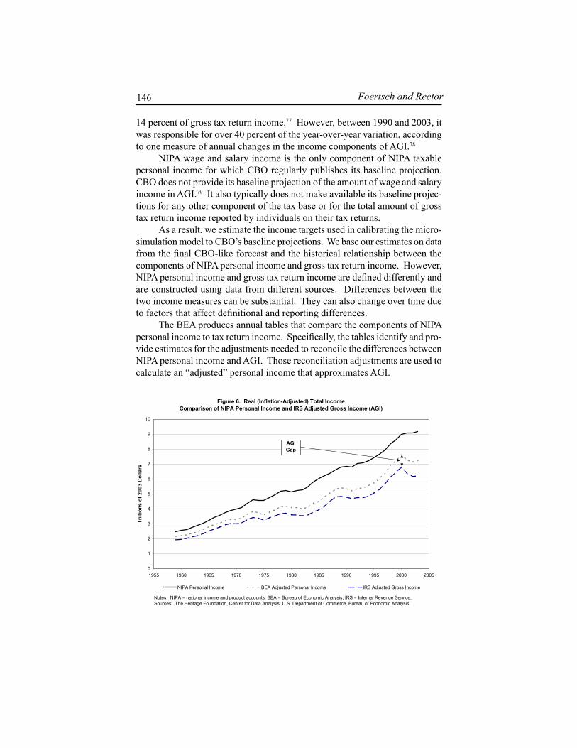
Foertsch and Rector 146
14 percent of gross tax return income.77 However, between 1990 and 2003, it was responsible for over 40 percent of the year-over-year variation, according to one measure of annual changes in the income components of AGI.78
NIPA wage and salary income is the only component of NIPA taxable personal income for which CBO regularly publishes its baseline projection. CBO does not provide its baseline projection of the amount of wage and salary income in AGI.79 It also typically does not make available its baseline projec-tions for any other component of the tax base or for the total amount of gross tax return income reported by individuals on their tax returns.
As a result, we estimate the income targets used in calibrating the micro-simulation model to CBO’s baseline projections. We base our estimates on data from the final CBO-like forecast and the historical relationship between the components of NIPA personal income and gross tax return income. However, NIPA personal income and gross tax return income are defined differently and are constructed using data from different sources. Differences between the two income measures can be substantial. They can also change over time due to factors that affect definitional and reporting differences.
The BEA produces annual tables that compare the components of NIPA personal income to tax return income. Specifically, the tables identify and pro-vide estimates for the adjustments needed to reconcile the differences between NIPA personal income and AGI. Those reconciliation adjustments are used to calculate an “adjusted” personal income that approximates AGI.
Figure 6. Real (Inflation-Adjusted) Total IncomeComparison of NIPA Personal Income and IRS Adjusted Gross Income (AGI)
0
1
2
3
4
5
6
7
8
9
10
1955 1960 1965 1970 1975 1980 1985 1990 1995 2000 2005
Trill
ions
of 2
003
Dol
lars
NIPA Personal Income BEA Adjusted Personal Income IRS Adjusted Gross Income
AGIGap
Notes: NIPA = national income and product accounts; BEA = Bureau of Economic Analysis; IRS = Internal Revenue Service.Sources: The Heritage Foundation, Center for Data Analysis; U.S. Department of Commerce, Bureau of Economic Analysis.

Calibrating Macroeconomic and Microsimulation Models 147
The difference remaining between adjusted personal income and AGI is called the “AGI gap.” The total AGI gap for real adjusted personal income and inflation-adjusted AGI increased gradually between 1960 and 2000 (see Figure 6). It increased more rapidly between 2000 and 2003. However, the BEA’s estimate of adjusted personal income captures most of the turning points in AGI. And differences between adjusted personal income and AGI are within ± 1.7 percent of the 12.3-percent mean difference for about two-thirds of the 45-year period shown in Figure 6.
The total AGI gap has been relatively constant in large part because the AGI gap for wage and salary income has been historically stable. The size of the total AGI gap is influenced by wage and salary income because wages and salaries account for the largest share of both personal income and AGI. In 2003, wages and salaries were over 53 percent of NIPA personal income before subtracting employee-paid social insurance contributions. They were almost 74 percent of gross tax return income in 2003 and over 86 percent of the components of NIPA personal income included in AGI.
The definitional differences between NIPA wage and salary income and wages and salaries included in gross tax return income are numerous (see Figure 7). The NIPA definition includes wages and salaries that are not taxable, such as
Figure 7. Components of Wage and Salary Adjustments In The NIPA - AGI Reconciliation
-$175
-$150
-$125
-$100
-$75
-$50
-$25
$0
$25
$501990 1991 1992 1993 1994 1995 1996 1997 1998 1999 2000 2001 2002 2003
Bill
ions
of 2
003
Dol
lars
OtherDisability Pensions Taxed As WagesEmployee 401k 403b 408kExempt Military PayTSP Employee PortionImputed Income
Notes: NIPA = national income and product accounts; AGI = adjusted gross income.Sources: The Heritage Foundation, Center for Data Analysis; U.S. Department of Commerce, Bureau of Economic Analysis.

Foertsch and Rector 148
more than double the historical average. Nevertheless, we can derive a rea-sonably close relationship between NIPA and AGI wage and salary income by developing separate estimates for the reconciliation adjustments and the remaining AGI gap.80
Figure 8. Real (Inflation-Adjusted) Wage and Salary IncomeComparison of NIPA Personal Income and IRS Adjusted Gross Income
0
1
2
3
4
5
6
1955 1960 1965 1970 1975 1980 1985 1990 1995 2000 2005
Trill
ions
of 2
003
dolla
rs
NIPA Personal Income BEA Adjusted Personal Income IRS Adjusted Gross Income
Notes: NIPA = national income and product accounts; BEA = Bureau of Economic Analysis; IRS = Internal Revenue Service.Sources: The Heritage Foundation, Center for Data Analysis; U.S. Department of Commerce, Bureau of Economic Analysis.
(some or tax-exempt) payments to military personnel, employee contributions to retirement programs (401K accounts, 403B accounts, TSP plans, etc.), and imputed estimates for noncash income. It also includes earnings for individu-als who do not file tax returns. However, it excludes income from disability pension plans and other sources included in taxable wages.
A comparison of the wage and salary components of adjusted personal income and IRS-reported AGI shows trends that are similar to those found in a comparison of total income (see Figure 8). For most of the period between 1960 and 2003, adjusted personal income moved in lock step with AGI wage and salary income, with a real mean overstatement of about 3.3 percent. As with total income, the AGI gap for wages and salaries in recent years has grown, in this case since 1996. By 2003, the adjusted personal income measure of wages and salaries overestimated its AGI equivalent by almost 7.5 percent,

Calibrating Macroeconomic and Microsimulation Models 149
In addition to being the largest component of NIPA personal income and AGI, wages and salaries constitute the greatest source of year-to-year variation in the NIPA-based portion of gross tax return income. For example, between 1990 and 2003, inflation-adjusted wages and salaries accounted for over 60 percent of the sum of annual absolute value changes in the income components of AGI that are also included in NIPA personal income.
Interest income is the second largest source of variation in the NIPA-based portion of AGI. Taxable interest accounted for around 15 percent of the absolute value of the inflation-adjusted annual change between 1990 and 2003. Unlike wages and salaries, the trend in interest income as measured in NIPA personal income is substantially different from the trend in interest income as measured in AGI. A large part of that difference may be attributed to the inclusion of imputed income in the NIPA--but not the AGI--measure of interest income. Imputed income comprised over 60 percent of NIPA personal interest in 2003.81
Even after subtracting imputed income and making other adjustments, some significant differences remain between the adjusted personal income measure of interest income and the AGI measure (see Figure 9). In general, the components of adjusted personal income, including interest income, are generally larger than the components of AGI. However, adjusted personal interest fell below the IRS measure in 1997 and 2000.
Figure 9. Real (Inflation-Adjusted) Interest IncomeComparison of NIPA Personal Income and IRS Adjusted Gross Income
0
200
400
600
800
1,000
1,200
1955 1960 1965 1970 1975 1980 1985 1990 1995 2000 2005
Bill
ions
of 2
003
dolla
rs
NIPA Personal Income BEA Adjusted Personal Income IRS Adjusted Gross Income (Taxable Only)
Notes: NIPA = national income and product accounts; BEA = Bureau of Economic Analysis; IRS = Internal Revenue Service.Sources: The Heritage Foundation, Center for Data Analysis; U.S. Department of Commerce, Bureau of Economic Analysis.

Foertsch and Rector 150
Dividend income is the third largest source of annual variation in the NIPA-based income portion of AGI. Between 1990 and 2003, dividend income was responsible for over 6.5 percent of the absolute value of the inflation-ad-justed annual change in the NIPA components of AGI. However, important differences exist between the NIPA and AGI definitions of dividend income. For example, some payments to the owners of small business corporations (S corporations) are included in personal dividend income but excluded from IRS dividends. Such definitional differences complicate estimation of the income targets needed to calibrate the microsimulation model.
Figure 10. Real (Inflation-Adjusted) Dividend IncomeComparison of NIPA Personal Income and IRS Adjusted Gross Income
0
50
100
150
200
250
300
350
400
450
1955 1960 1965 1970 1975 1980 1985 1990 1995 2000 2005
Bill
ions
of 2
003
Dol
lars
NIPA Personal Income BEA Adjusted Personal Income IRS Adjusted Gross Income
Notes: NIPA = national income and product accounts; BEA = Bureau of Economic Analysis; IRS = Internal Revenue Service.Sources: The Heritage Foundation, Center for Data Analysis; U.S. Department of Commerce, Bureau of Economic Analysis.
Even after the reconciliation adjustments are taken into account, both the level and movement of dividends in gross tax return income and NIPA personal income are noticeably different (see Figure 10). For example, between 2001 and 2002, AGI dividends fell by over $18 billion while the adjusted personal income measure of dividends showed an increase of over $20 billion, in infla-tion-adjusted terms.
In general, a comparison of wage and salaries in adjusted personal income and AGI suggests a much closer relationship than evidenced for either inter-est income or dividend income. As a result, income estimates based on NIPA values are likely to be less accurate for the interest and dividend components of gross tax return income than they are for wages and salaries. Contributing to

Calibrating Macroeconomic and Microsimulation Models 151
any potential inaccuracies, the Global Insight model does not include variables that can be used to estimate the reconciliation adjustments made by BEA when comparing NIPA personal income and IRS-reported AGI.
The effect of these limitations can be seen by comparing the actual amounts of gross tax return income and the estimated amounts obtained us-ing a regression based on the historical relationships between the NIPA and tax measures. Most of the predicted amounts are close to their actual values. However, there are noticeable exceptions. For example, between 1993 and 1994, IRS interest income (including the nontaxable portion) was estimated to increase by roughly $20 billion to $191 billion (see Figure 11). Instead, actual IRS interest income fell by around $4 billion to $174 billion. Estimated dividend income in AGI and actual dividend income in AGI likewise diverged for several years between 1990 and 2003 (see Figure 12).
The paragraphs above discuss how we use NIPA data to estimate the amount of wage and salary income, dividend income, and interest income re-ported on tax returns. We use similar techniques to estimate other NIPA-based components of gross tax return income. Those components include proprietors’ (farm and nonfarm) gains and net losses, income from rents and royalties, and income from trusts and estates. We also estimate net passthrough income from S corporations that is included in NIPA corporate profits.82 Social Security income is introduced as a separate target because a portion of Social Security benefits are included in taxable income.
The sum of our forecasts of the components of NIPA-based income and non-NIPA-based income approximates the taxable income base that CBO uses to project Federal receipts from the individual income tax. CBO does not pro-vide its projections for most of the components of gross tax return income. As a result, there can be differences between income amounts we use and those projected by CBO. We do not have any information about the size of those differences, or whether they even exist, until we calculate Federal revenues in the final step of the calibration process.
In the final step, we adjust a set of nonincome variables used to calculate taxes in the model and introduce additional distributional targets. The nonin-come variables include itemized deductions and some statutory adjustments.83 We compare CBO’s projections of individual income tax collections with estimates of tax liability that are calculated by the microsimulation model and adjusted to reflect the timing of tax payments. Tax payments are divided into withholding, estimated payments, and final payments. The payments are ag-gregated to estimate fiscal year revenue collections. An additional adjustment is made to reflect payments for fees, penalties, and other collections. When there are material differences in the revenue projections, we modify our targets

Foertsch and Rector 152
Figure 11. Actual IRS Total Interest Income vs. Estimated IRS Total Interest Income
100
120
140
160
180
200
220
240
260
280
1990 1991 1992 1993 1994 1995 1996 1997 1998 1999 2000 2001 2002 2003
Bill
ions
of d
olla
rs
Notes: IRS = Internal Revenue Service.Sources: The Heritage Foundation, Center for Data Analysis; U.S. Department of Commerce, Bureau of Economic Analysis.
Actual IRS
Estimated IRS
Figure 12. Acutal AGI Dividend Income vs. Estimated AGI Dividend Income
40
60
80
100
120
140
160
1990 1991 1992 1993 1994 1995 1996 1997 1998 1999 2000 2001 2002 2003
Bill
ions
of d
olla
rs
Notes: AGI = adjusted gross income.Sources: The Heritage Foundation, Center for Data Analysis; U.S. Department of Commerce, Bureau of Economic Analysis.
Actual AGI
Estimated AGI

Calibrating Macroeconomic and Microsimulation Models 153
for the distribution of gross tax return income by size of income and by marital filing status.
Adjustments may be needed because a large proportion of the total Federal income tax is paid by a relatively small proportion of taxpayers at the top end of the income distribution. Slight changes in assumptions about the number of tax returns in the top classes can produce significant changes in total rev-enue projections. We do not know CBO’s projections for the distribution of income or tax collections by detailed income class. We therefore adjust targets for both distributional variables in the final stage of calibrating the model so that estimates of total income tax collections from the microsimulation model approximate CBO’s published projections.84
Implications for Tax Policy SimulationsAn integrated calibration of the macroeconomic and microsimulation models provides a consistent basis for conventional tax policy analysis. The final CBO-like forecast replicates CBO’s published projections. It also includes projections of key components of NIPA personal income not typically published by CBO. The microsimulation model uses the final CBO-like forecast to gen-erate current-law estimates of the Federal income tax over a 10-year period. It includes detailed estimates by income class of gross tax return income on individual tax returns and nontaxable income as reported on the CPS. Those estimates of taxable and nontaxable income are consistent with components of NIPA personal income obtained from the final CBO-like forecast.
Calibrating the Global Insight model and the microsimulation tax model to a common starting point also produces a consistent basis for dynamic policy analysis. This is because an integrated calibration allows us to make direct comparisons between dynamically and conventionally estimated changes in Federal income tax revenues. It also assures us that dynamic revenue estimates from the Global Insight model are broadly consistent with the microsimulation model’s conventional estimates of revenue and distributional effects.
Our tax policy simulations broadly proceed in three separate steps once we have calibrated the Global Insight model and the microsimulation model to CBO’s baseline projections.
First, we use the microsimulation model to obtain a conventional estimate of the revenue effects of a proposed change in tax policy. That proposed tax policy can involve a change in current-law Federal income tax rates or provi-sions or a change in the Federal personal income tax base. The microsimula-tion model is used to make a conventional estimate of the implied change in Federal income tax revenues. It also produces estimates of marginal tax rates

Foertsch and Rector 154
on three types of income--ordinary income, long-term capital gain realizations, and dividend income--under the proposed policy.
Second, we use the Global Insight model to estimate the dynamic revenue effects of the same policy change. We use conventionally estimated changes in Federal tax revenues and marginal tax rates under current law and the proposed policy as inputs in a simulation with the Global Insight model. That simulation produces an alternative to the CBO-like baseline forecast. That alternative (nonbaseline) forecast includes the dynamic effects of the proposed policy on GDP, prices, interest rates, employment, and personal and corporate incomes, among other variables. Revenue feedbacks can be calculated as the difference between the dynamically estimated change in Federal income tax revenues from the Global Insight model and the conventionally estimated change in the same from the microsimulation model.
Third, we update the microsimulation model to reflect the dynamic effects of the proposed tax policy on individual income. We update individual income in the microsimulation model using similar procedures developed for baseline calibration. Thus, NIPA components of personal and corporate income along with price-level variables and some NIPA budget variables from the alterna-tive forecast are used to estimate target values for gross tax return income on individual income tax returns and nontaxable income reported on the CPS. We use those targets to set individual income in the microsimulation model so that they are consistent with the Global Insight model’s alternative forecast for the components of NIPA personal income.
We compare dynamically and conventionally estimated changes in Federal tax revenues when evaluating results from the Global Insight model and the microsimulation model.85 We consider the tax-policy simulation complete if differences between the Global Insight model’s dynamically estimated changes and the microsimulation model’s conventionally estimated changes in Federal tax revenues can be accounted for by initial differences in the Federal personal income tax bases in the two models.
In practice, we regularly calibrate both the Global Insight model and the microsimulation model to CBO’s baseline projections. We also regularly use the calibrated macroeconomic and microsimulation models to analyze a variety of tax proposals. In some instances, tax data in the microsimulation model provide a “stand-alone” conventional revenue estimate. In other instances, the conventional revenue estimate is input into the Global Insight model to generate a “first-round” dynamic estimate of the economic and budgetary ef-fects of the tax proposal. For a handful of major tax proposals, we have used the “first-round” dynamic estimate to re-age the matched file to reflect the new alternative forecast from the Global Insight model. When we have done so, we have iterated between the Global Insight model and the microsimulation model until the two models have produced similar revenue results.86

Calibrating Macroeconomic and Microsimulation Models 155
AcknowledgmentsTracy L. Foertsch, Ph.D., is a Senior Policy Analyst, and Ralph A. Rector, Ph.D., is a Senior Research Fellow and Project Manager in the Center for Data Analysis at The Heritage Foundation. The useful comments of Mark A. Led-better (Bureau of Economic Analysis), Christopher Williams (Congressional Budget Office), Mark Lasky (Congressional Budget Office), and Rosemary Marcuss (Deputy Director of the Bureau of Economic Analysis) are gratefully acknowledged. The authors thank Ben Keefer and Kevin Kellert for their re-search assistance and Richard Odermatt for his editorial assistance. All errors and omissions remain the responsibility of the authors.
Endnotes 1 The methodologies, assumptions, conclusions, and opinions presented
here have not been endorsed by and do not necessarily reflect the views of the owners of the Global Insight model or their employees. Fortune 500 companies and numerous Government agencies use Global Insight’s short-term U.S. Macroeconomic Model to forecast how changes in the economy and in public policy are likely to affect major economic indica-tors. The Global Insight model is calibrated to, and used to forecast, national income and product accounts (NIPA) economic and budget-ary data. CBO’s baseline projections include short-term forecasts and medium-term projections of largely the same economic and budgetary variables.
2 See Joint Committee on Taxation (2005) for additional details. 3 Even these rankings will be problematic if they are sensitive to assump-
tions in the baseline that are contrary to current economic conditions. 4 See CBO (2006) and previous releases of CBO’s The Budget and Eco-
nomic Outlook for additional details on CBO’s procedures for projecting Federal revenues and spending beyond 1 year under current-law as-sumptions. See Williams (2005b) for a summary of the rules governing CBO’s current-law Federal budget baseline.
5 Under JGTRRA, individual long-term net capital gain realizations and qualified dividend income are taxed at preferential rates. Taxpayers with taxable income in the lowest two tax brackets pay a 5-percent tax rate on capital gains and dividend income through 2007 and a 0-percent tax rate on capital gains and dividend income in 2008. Taxpayers with tax-able income in all other tax brackets pay a 15-percent tax rate on capital gains and dividend income through 2008. JGTRRA’s preferential tax

Foertsch and Rector 156
rates on capital gains and dividend income were set to expire at the end of Calendar Year 2008. The Tax Increase Prevention and Reconciliation Act of 2005 extends JGTRRA’s preferential rate structure through the end of 2010. Taxes on both types of capital income will revert to their pre-JGTRRA levels in 2011. This means that, with no further exten-sions, dividend income will be taxed at ordinary income tax rates, while capital gains realizations will be taxed at a pre-JGTRRA maximum rates of 10 percent and 20 percent.
6 Those tax relief provisions in EGTRRA that are expiring in 2010 include the reduction in marginal tax rates on the top two income tax brackets, the new 10-percent income tax bracket, the $1,000 child tax credit, and the phaseout of the estate tax. See Joint Committee on Taxation (2001) for additional information.
7 “Budget period” here refers to the time horizon used either to project baseline, current-law revenues or to estimate the revenue effects of a change in current law. A 10-year period is standard in the Federal bud-get process.
8 CBO (2006, pp. 65-74) projects that education, training, and employ-ment; transportation; health research and public health; and income security (primarily housing and food assistance programs) will account for over half of nondefense discretionary spending in 2006.
9 Supplemental appropriations typically provide budget authority in response to events not anticipated during the regular budget cycle (CBO, 2006, pp. 69-70). Supplemental appropriations in Fiscal Year 2005 totaled $157 billion. They included $82 billion for defense and tsu-nami relief (the 2005 Emergency Supplemental Appropriations Act for Defense, the Global War on Terror, and Tsunami Relief) and $62 billion in response to Hurricanes Katrina and Rita. Section 257 of the Bal-anced Budget and Emergency Deficit Control Act of 1985 sets the rules covering CBO’s treatment of discretionary spending and supplemental appropriations in a current-law baseline.
10 See Williams (2005b).11 CBO’s 2-year economic forecasting record compares favorably to that
of the Blue Chip consensus and the Office of Management and Budget (OMB). See Williams (2005a) for a recent analysis of CBO’s economic forecasting record.
12 See CBO (2003, pp. 38-41).

Calibrating Macroeconomic and Microsimulation Models 157
13 See CBO (2003, pp. 25-26, 29-36).14 CBO’s growth model is an enhanced version of the model developed by
Robert Solow. Arnold (2001, 2004) provides additional details.15 See CBO (2006, Table E-1, p. 136).16 Throughout this paper, we compare CBO’s baseline economic and bud-
getary projections to Global Insight’s (standard) February 2006 short-term U.S. Macroeconomic forecast. This is because the latter is used as a starting point (control forecast) in constructing a CBO-like forecast from the Global Insight model. See Global Insight (2006) for additional details on GI’s February 2006 forecast. A subscription is required to download Global Insight’s February 2006 U.S. Economic Outlook.
17 See Brauer (2004).18 See Williams (2005b) and Dennis (2004).19 See Global Insight (2006, pp. 53-59). A subscription is required to
download Global Insight’s February 2006 US Economic Outlook.20 Specifically, NIPA Federal defense spending declined at an annual rate
of 12.7 percent in the fourth quarter of 2005 after expanding at an annual rate of almost 13.9 percent in the third quarter of the same year.
21 Congress did not approve the Fiscal Year 2006 defense spending appro-priations bill until December 21, 2005.
22 In fact, CBO (2006, p. 37) expects Federal military purchase to slow under current law in 2007.
23 Brian Bethune, Director of Financial Economics in Global Insight’s U.S. Macroeconomics Group, provided information on GI’s baseline assump-tions for Federal defense spending.
24 For 2006, CBO (2006, Box 2-2, pp. 34-35) put the applicable ERISA discount rate at 5.15 percent and DB contributions at $185 billion. Had PFEA been extended, a maximum applicable discount rate of 5.75 percent would have applied under CBO’s baseline projections. At that higher discount rate, DB contributions would have totaled only $135 billion.
25 Brian Bethune, Director of Financial Economics in Global Insight’s U.S. Macroeconomics Group, provided information on the extent to which GI’s projections of corporate (book) profits reflect PFEA’s expiration.
26 GI’s February 2006 U.S. Macroeconomic forecast is used as the control because it was prepared over roughly the same time period as CBO’s

Foertsch and Rector 158
January 2006 baseline projections. Using a control forecast prepared over roughly the same time period is particularly important if the BEA revises the NIPA data. For CBO’s January 2006 baseline projections, either GI’s December 2005 forecast or its January 2006 forecast might have made a better choice for the control. However, we selected the February 2006 forecast because it was the first to include 2016 in the 10-year forecast horizon.
27 CBO (2006, Appendix D, pp. 125-134) and Russek (2005) provide a single crosswalk table summarizing the coverage, netting, and timing differences between total unified Federal budget aggregates (revenues, outlays, and surpluses) and total NIPA Federal budget aggregates (re-ceipts, expenditures, and net Government saving). The structure of that crosswalk table is similar to Tables 4 and 5 in Mandel and Roy (2006).
28 NIPA taxable personal income is the sum of NIPA wage and salary income, personal interest income, personal rental income, personal divi-dend income, and proprietors’ income (farm and nonfarm).
29 The exception is CBO’s estimate for the natural rate of unemployment, which also equals CBO’s medium-term projection of the unemployment rate. In January 2006, CBO (2006, Chapter 2, p. 43) put the natural rate of unemployment at 5.2 percent.
30 See CBO (2005, Chapter 2, pp. 37-41).31 See CBO (2006, Chapter 2, p. 39).32 See CBO (2005, Chapter 2, pp. 36).33 See CBO (2006, Chapter 2, p. 41).34 Specifically, Figures 4 and 5 reorganize NIPA data into a simple social
accounting framework. Although generally used most extensively in input-output analysis and computable general equilibrium modeling, a social accounting framework underlies all systems of national accounts. See United Nations (1993) for additional details.
35 The microsimulation model also requires targets for types of individual income that are not included in NIPA personal income.
36 For its August 2006 economic and budgetary projections, CBO pub-lished a separate background paper (Mascaro, 2006) discussing how it forecasts the components of gross domestic income. This is the first time CBO has published details about its methodology for forecasting NIPA income variables.

Calibrating Macroeconomic and Microsimulation Models 159
37 See CBO (2006, Table 4-4, p. 92).38 The appendix to an earlier, unpublished draft of this paper shows how
closely the final CBO-like forecast reproduces key economic-and-bud-getary projections published by CBO. It also details the implications of those projections for components of GDP and NIPA taxable personal income. The appendix is available on request.
39 Global Insight provided a detailed outline of a methodology for calibrat-ing the GI model to CBO’s baseline projections. We created a series of AREMOS programs based on that outline, making adjustments and additions to GI’s basic methodology where appropriate. AREMOS is Global Insight’s proprietary econometric analysis and modeling soft-ware.
40 Unless otherwise indicated, projections of all Federal outlay variables are taken from Table D-1 and Table D-2 of CBO (2006, Appendix D, pp. 128-129, 133).
41 CBO’s baseline projection of Federal net investment is labeled “Treat-ment of investment and depreciation” in Table D-1 of CBO (2006, Ap-pendix D, pp. 128-139). It is part of the total difference between NIPA and unified Federal outlays.
42 See CBO (2006, Table 3-1, p. 52) and NIPA Table 3.12 (U.S. Depart-ment of Commerce, 2006).
43 For example, in January 2006, CBO (2006, p. 33) forecast that “real consumer spending will grow at a 3.5-percent rate this year and in 2007.”
44 See CBO (2006, Table 2-2, p. 44). For the nonfarm business sector, CBO also publishes medium-term projections of annual average rates of growth in potential hours worked and potential capital. We have not yet exploited these additional published projections in calibrating the Global Insight model to CBO’s current-law baseline.
45 CBO published historical estimates of potential output since 1950, along with projections of potential output through 2011 in Arnold (2001).
46 See CBO (2006, Table 4-3, p. 86). CBO typically does not publish pro-jections of NIPA taxable personal income in its August update.
47 The appendix to an earlier, unpublished draft of this paper shows the implications of CBO’s baseline economic-and-budgetary projections for the personal saving rate. The appendix is available on request.

Foertsch and Rector 160
48 Contributions for Federal social insurance are an important component of NIPA Federal tax receipts. We set contributions for Federal social insurance to be consistent with CBO’s baseline revenue projections in step 1. We do so by calculating the Federal social insurance tax rate as the divisor of CBO’s projections of Federal social insurance tax receipts and wage and salary income.
49 See CBO (2006, Table 4-4, p. 92) for CBO’s projections of individual capital gain realizations.
50 See Petrick (2002) for additional information on how BEA estimates corporate profits in the NIPA.
51 Specifically, the Global Insight model defines corporate (book) profits as GNP net of, among other variables, consumption of fixed capital (corpo-rate and noncorporate), taxes on production and imports (Federal as well as State and local), transfer payments by businesses, interest payments by businesses, employer-paid payroll taxes, fringe benefits, wage and salary incomes, proprietors’ incomes, and personal rental income.
52 We calculate average effective Federal tax rates on personal and cor-porate incomes as the divisor of CBO’s projections of Federal personal and corporate income tax revenues and our projections of the Federal personal and corporate income tax bases.
53 Before imposing targets for either publicly-held Federal debt or net Federal interest payments, we adjust individual components of Federal spending so that only gross Federal interest payments account for any deviation in the CBO-like forecast from CBO’s published projections of NIPA Federal spending.
54 Federal income on assets is the sum of Federal interest income and Federal rent and royalty receipts. We calculate net Federal interest pay-ments as the difference between gross Federal interest payments and Federal interest income.
55 See Weber (2004) for information on the most recent (2001) Public-Use Tax File. SOI has issued public-use files for almost every year since 1960.
56 Data fields here refer to individual lines on IRS Form 1040 and on sup-porting schedules and forms.
57 However, tables published by the IRS do show aggregate amounts of foreign-earned income within the adjusted gross income classes. For

Calibrating Macroeconomic and Microsimulation Models 161
additional details, see Table 1-4 (Individual Income Tax, All Returns: Sources of Income, Adjustments, and Tax Items, by Size of Adjusted Gross Income) of IRS (2005) at http://www.irs.gov/pub/irs-soi/03in14ar.xls.
58 For example, see Sailer and Weber (1996).59 The CPS is a monthly survey of about 50,000 households conducted by
the Bureau of the Census for the Bureau of Labor Statistics (BLS). The CPS provides estimates of employment, earnings, hours of work, and other labor force characteristics by a variety of demographic characteris-tics, including age, gender, and race. Supplemental questions to the CPS provide additional information on education, health, and employee ben-efits. For a general overview of the design and methodology of the CPS, see U.S. Census Bureau and BLS (2002). For a general overview of the Annual Demographic Survey (March CPS Supplement), see http://www.bls.census.gov/cps/ads/adsmain.htm.
60 See U.S. Census Bureau (2005) for additional information. The Census Bureau now calls the special supplement of the March CPS the CPS ASEC, although it is still widely referred to as the March CPS supple-ment.
61 The SOI and CPS matched file constitutes the core base-year data used in the microsimulation model. However, data from other sources includ-ing the Survey of Consumer Finance (SCF) and the Consumer Expen-diture Survey (CEX) provide additional information used in the micro-simulation model.
62 The matching algorithm searches for the combination of CPS and SOI records that minimizes differences for a set of variables found on both files. These variables include sources of income, the presence and relative size of income components common to the SOI and CPS, and marginal statutory tax rates. A normalized Z score is used to take into account differences in the distribution of income (by source) on SOI and CPS records. Adjustments are also made for income that is top-coded on the CPS and for differences in the number of records that contain nonzero values. A separate search is performed within each partition. In some instances, minimizing the overall difference within a partition requires that a record be split so that multiple copies are produced. For example, a CPS record might be duplicated and then matched with two separate SOI records. If this occurs, the weights are modified so that

Foertsch and Rector 162
they sum to the prematched total. In addition, the algorithm ensures that the weights for records within the same family will be equal even when the returns are in different partitions.
63 For married couples, CPS data are used to allocate payroll taxes between spouses.
64 The parameter input file specifies a set of variables (or equations incor-porating variables) to be included in the report. The selection criteria allow the data by record characteristics to be summarized by tax year, size of income, and a wide combination of tax return characteristics.
65 Two of the most important publications are SOI’s (annual) Publica-tion 1304 reports (IRS, 2005) and an SOI report giving the percentile distribution of AGI and tax generated for individual income tax returns (Mudry and Parisi, Table 5, 2006). We also rely on SOI Bulletin articles on partnerships (Wheeler and Shumofsky, 2005), S corporations (Lut-trell, 2005), and sole proprietorships (Pierce, 2005).
66 The CPS also provides historical population data.67 NIPA income data are available with less of a lag than tax return data
published by the SOI.68 For example, see Hussain (2006).69 See U.S. Census Bureau (2006).70 Gross tax return income here refers to a broad income measure that
approximates the Internal Revenue Code’s definition of gross income reported on Form 1040.
71 For additional information on the PSID, see http://www.psidonline.isr.umich.edu/.
72 Individual characteristics here include age, sex, marital status, share of income by type, and the level of income. Key economic indicators include GDP and employment.
73 Income data taken from the tax returns are first disaggregated to the person level and then used to compute income targets by percentile.
74 Income targets for those with negative Federal AGI are estimated using both projections of losses in the current year and losses carried forward from prior years.
75 In estimating detailed personal income targets, we rely on unpub-lished detailed tables comparing the components of Personal Income

Calibrating Macroeconomic and Microsimulation Models 163
and Adjusted Gross Income. Those tables are available from BEA on request. We refer to them here as the “AGI Personal Income 1959-2003” workbook. We also rely on annual Survey of Current Business articles describing the major categories used to reconcile the differences be-tween NIPA personal income and IRS Federal adjusted gross income. Ledbetter (2004) provides additional details. For a summary of a recent reconciliation of NIPA personal income and IRS Federal AGI, see NIPA Table 7.19 (U.S. Department of Commerce, 2005). Table 7.19 appears periodically in the Survey of Current Business.
76 We obtain historical values for, and projections of, capital gain realiza-tions from, CBO (2006, Table 4-4, p. 92). We develop independent estimates for the remaining non-NIPA sources of personal income.
77 This percentage includes income from S corporations which is not in-cluded in NIPA personal income but is included in corporate profits. S corporation income accounted for about 2.4 percent of gross tax return income in 2003.
78 Non-NIPA income components account for about 41.3 percent of the sum of the absolute value of inflation-adjusted annual changes in the components of tax return income between 1990 and 2003. This excludes net S corporation income although a portion of this income is included in the NIPA measure of personal divident income. These and the remaining calculations in this section are based on data from the “AGI Personal Income 1959-2003” workbook and the authors’ calculations.
79 A CBO background paper (Mascaro, 2006) discusses how CBO fore-casts the components of NIPA gross domestic income for its August 2006 economic and budgetary projections. However, that paper does not include details about CBO’s methodology for linking forecasted NIPA income with measures of gross tax return income.
80 For 1990 through 2003, the adjusted R squared is 0.985 for a standard OLS estimate of the relationship between the reconciliation adjustment and the NIPA values of wages and salaries and military pay. The adjust-ed R squared is 0.988 for an OLS estimate of the relationship between the AGI gap for wage and salary income and NIPA wages and salaries and military pay.
81 The two imputations are for investment income that is retained by life insurance carriers and pension plans and services that noninsurance financial intermediaries provide without payment (Ledbetter, 2004).

Foertsch and Rector 164
82 NIPA does not separately report the sum of gains and losses for sole proprietorships or other businesses. Losses are instead added to gains to derive an aggregate net amount of proprietorship income. This is prob-lematic for purposes of estimating Government revenues because taxes are only paid on positive income. We therefore use IRS data to estimate the historical relationship between the aggregate amount of proprietors’ income and the amount of net gains and losses.
83 We estimate growth rates to age many of these nonincome variables.84 More specifically, we target Federal individual income tax revenues that
have been adjusted to reflect definitional and timing differences between the tax liability reported on tax returns and CBO’s published revenue collections.
85 We isolate changes in Federal personal income tax revenues and Federal corporate income tax revenues when comparing budgetary projections from the Global Insight model and the microsimulation model.
86 For example, see Foertsch and Rector (2007).
ReferencesArnold, Robert (2004), “A Summary of Alternative Methods for Estimating
Potential GDP,” Congressional Budget Office Background Paper, March. http://www.cbo.gov/ftpdocs/51xx/doc5191/03-16-GDP.pdf.
Arnold, Robert (2001), “CBO’s Methods for Estimating Potential Output: An Update,” A Congressional Budget Office Paper, August. http://www.cbo.gov/ftpdocs/30xx/doc3020/PotentialOutput.pdf.
Brauer, David (2004), “CBO’s Projections of the Labor Force,” Congres-sional Budget Office, September. http://www.cbo.gov/ftpdocs/58xx/doc5803/09-15-LaborForce.pdf.
Congressional Budget Office (2006), The Budget and Economic Outlook: Fiscal Years 2007 to 2016, January. http://www.cbo.gov/ftpdocs/70xx/doc7027/01-26-BudgetOutlook.pdf.
Congressional Budget Office (2005), The Budget and Economic Outlook: An Update, August. http://www.cbo.gov/ftpdocs/66xx/doc6609/08-15-OutlookUpdate.pdf.

Calibrating Macroeconomic and Microsimulation Models 165
Congressional Budget Office (2003), The Budget and Economic Outlook: An Update, August. http://www.cbo.gov/ftpdocs/44xx/doc4493/08-26-Report.pdf.
Dennis, Robert et al. (2004), “Macroeconomic Analysis of a 10-Percent Cut in Income Tax Rates,” Congressional Budget Office Technical Paper Series, 2004-07, May. http://www.cbo.gov/ftpdocs/54xx/doc5485/2004-07.pdf.
Foertsch, Tracy L. and Rector, Ralph A. (2007), “A Dynamic Analysis of Permanently Extending EGTRRA and JGTRRA: An Application of a Co-ordinated Calibration of Macroeconomic and Microsimulation Models,” The 15th Federal Forecasters Conference--2006: Papers and Proceedings, forthcoming.
Global Insight (2006), “U.S. Economic Outlook,” February. http://myinsight.globalinsight.com/servlet/cats?pageContent=fileList&serviceID=1784&typeID=P&resourceID=4477&archive=1 or http://myinsight.globalinsight.com/servlet/cats?pageContent=downloadFile&file=106453.pdf.
Hussain, Taukir (2006), “Projections of Federal Tax Return Filings: Calen-dar Years 2005-2012,” SOI Bulletin, Winter, pp. 147-156.http://www.irs.gov/pub/irs-soi/12proj.pdf.
Internal Revenue Service (2005), “Statistics on Income--2003 Individual Income Tax Returns Publication 1304 (Rev. 09-2005), September. http://www.irs.gov/taxstats/article/0,,id=134951,00.html.
Internal Revenue Service (2005), “Statistics of Income--2003 Individual Income Tax Returns Publication 1304 (Rev. 09-2005), Table 1.4, Septem-ber. http://www.irs.gov/taxstats/indtaxstats/article/0,,id=134951,00.html.
Joint Committee on Taxation (2005), “Overview of Revenue Estimating Pro-cedures and Methodologies Used by the Staff of the Joint Committee on Taxation,” JCX-1-05, February 2, pp. 18-19. http://www.house.gov/jct/x-1-05.pdf.
Joint Committee on Taxation (2001), “Summary of Provisions Contained in the Conference Agreement for H.R. 1836, The Economic Growth and Tax Relief Reconciliation Act of 2001,” JCX-50-01, May. http://www.house.gov/jct/x-50-01.pdf.

Foertsch and Rector 166
Ledbetter, Mark A. (2004), “Comparison of BEA Estimates of Personal Income and IRS Estimates of Adjusted Gross Income, New Estimates for 2001, Revised Estimates for 1959-2000,” Survey of Current Busi-ness, April, pp. 8-22. http://www.bea.gov/bea/ARTICLES/2004/04April/0404PI&AG.pdf.
Luttrell, Kelly (2005), “S Corporation Returns, 2002” SOI Bulletin, Spring, pp. 59-113. http://www.irs.gov/pub/irs-soi/02scorp.pdf.
Mandel, Benjamin A. and Roy, Mary L. (2006), “Federal Budget Estimates for Fiscal Year 2007,” Survey of Current Business, March, pp. 12-22. http://www.bea.gov/bea/ARTICLES/2006/03March/0306_Budget.pdf.
Mascaro, Angelo (2006), “How CBO Forecasts Income,” Congressional Budget Office Background Paper, August. http://www.cbo.gov/ftpdocs/75xx/doc7507/08-25-Income.pdf.
Mudry, Kyle and Parisi, Michael (2006), “Individual Income Tax Rates and Shares, 2003,” SOI Bulletin, Winter, pp. 18-56. http://www.irs.gov/pub/irs-soi/03inrate.pdf.
Petrick, Kenneth A. (2002), “Corporate Profits: Profits Before Tax, Profits Tax Liability, and Dividends,” Bureau of Economic Analysis Methodol-ogy Paper, September. http://www.bea.gov/bea/ARTICLES/NATIONAL/NIPA/Methpap/Methpap2.pdf.
Pierce, Kevin, (2005), “Sole Proprietorship Returns, 2003” SOI Bulletin, Summer, pp. 8-66. http://www.irs.gov/pub/irs-soi/03solp.pdf.
Russek, Frank (2005), “The Treatment of Federal Receipts and Expenditures in the National Income and Product Accounts,” A CBO Report, Congres-sional Budget Office, September. http://www.cbo.gov/ftpdocs/66xx/doc6625/09-02-NIPAs.pdf.
Sailer, Peter and Weber, Michael (1996) “Creating Household Data for Individual Income Tax Returns,” Proceedings, Section on Government Statistics, American Statistical Association.
U.S. Census Bureau (2006), “U.S. Interim Projections by Age, Sex, Race, and Hispanic Origin.” http://www.census.gov/ipc/www/usinterimproj.

Calibrating Macroeconomic and Microsimulation Models 167
U.S. Census Bureau (2005), “Current Population Survey, 2005 Annual Social and Economic (ASEC) Supplement, March. http://www.census.gov/apsd/techdoc/cps/cpsmar05.pdf.
U.S. Census Bureau and Bureau of Labor Statistics (2002), “Current Population Survey: Design and Methodology,” Technical Paper 63RV (TP63RV), March. http://www.census.gov/prod/2002pubs/tp63rv.pdf.
U.S. Department of Commerce, Bureau of Economic Analysis, National Income and Products Accounts (2006), Table 3.12 (Government Social Benefits), August. http://www.bea.gov/bea/dn/nipaweb/SelectTable.asp?Selected=N#S3.
U.S. Department of Commerce, Bureau of Economic Analysis, National Income and Product Accounts (2005), Table 7.19 (Comparison of Per-sonal Income in the National Income and Product Accounts with Adjusted Gross Income as Published by the Internal Revenue Service), September. http://www.bea.gov/bea/dn/nipaweb/SelectTable.asp?Selected=N#S7.
United Nations (1993), System of National Accounts 1993, Chapter XX (“Social Accounting Matrices”), United Nations, New York.http://unstats.un.org/unsd/sna1993/toctop.asp?L1=20.
Weber, Mike (2004), Individual Statistics Branch, Statistics of Income Divi-sion, Internal Revenue Service, General Description Booklet for the 2001 Public-Use Tax File, October. http://www.nber.org/~taxsim/gdb/gdb01.pdf.
Wheeler, Tim and Shumofsky, Nina (2005), “Partnership Returns, 2003,” SOI Bulletin, Fall, pp. 50-129. http://www.irs.gov/pub/irs-soi/03partnr.pdf.
Williams, Christopher (2005a), CBO’s Economic Forecasting Record: An Evaluation of the Economic Forecasts CBO Made from January 1976 through January 2003, October. http://www.cbo.gov/ftpdocs/68xx/doc6812/10-25-EconomicForecastingRecord.pdf.
Williams, Christopher (2005b), “What is a Current-Law Economic Base-line?”, Congressional Budget Office Economic and Budget Issue Brief, June. http://www.cbo.gov/ftpdocs/64xx/doc6403/EconomicBaseline.pdf.

Foertsch and Rector 168
Table 1. CBO’s January 2006 Baseline Economic and Budgetary Projections Used in Constructing the CBO-Like Baseline Forecast
Nominal GDP Billions of DollarsNominal GDP Percentage ChangeReal GDP Percentage ChangeGDP Price Index Percentage ChangeConsumer Price Index, All Urban Consumers Percentage ChangeCore Consumer Price Index Percentage ChangeUnemployment Rate PercentThree-Month Treasury Bill Rate PercentTen-Year Treasury Note Rate PercentCorporate Book Profits Billions of DollarsWages and Salaries Billions of DollarsPotential GDP Average Annual Growth RatePotential Labor Force Average Annual Growth Rate
Federal Expenditures/Outlays Federal Receipts/RevenuesConsumption Expenditures Current Tax Receipts Defense Consumption of Fixed Capital Taxes from ROW Non-defense Consumption of Fixed Capital Taxes on Production and Imports Defense Consumption Personal Income Tax Receipts Non-defense Consumption Corporate Income Tax ReceiptsGross Investment Contributions for Government Social Insurance
Federal Net Investment (defense and non-defense combined)
Social Insurance Tax Receipts
Transfer Payments Other Current Receipts Social Security Transfer Receipts Medicare Surpluses of Federal Government Sponsored Enterprises Social Benefits to the ROW Income on Assets Medicaid Federal Interest Payments Grants-in-Aid to State and Local Governments Gross Interest Payments Other Transfer Payments to ROW Publicly held Federal DebtSubsidies Debt Held by Government Accounts
Subsidies (agriculture, housing, all other combined) Unified (Budget) Surpluses/Deficits Other Means of Financing Publicly Held Federal Debt
Total Difference between NIPA expenditures and Unified Outlays
Total Difference between NIPA Receipts and Unified Revenues
Notes: CBO = Congressional Budget Office; NIPA = national income and product accounts; GI = Global Insight; ROW = rest of the world.
An earlier, unpublished draft of this paper includes more detailed notes to Table 1. Those notes are available uponrequest.
Sources: The Heritage Foundation, Center for Data Analysis, Congressional Budget Office.
All Baseline Economic Projections
Selected Baseline Budgetary Projections (Billions of Dollars)
Federal Reconciliation Items

The subject of this paper is to describe a new methodology of imputing tax variables to the Annual Social and Economic Supplement (ASEC) to the Current Population Survey (CPS). The U.S. Census Bureau had
produced Federal and State tax estimates each year since 1979 for the ASEC.1 These tax estimates are used to compute after-tax income. Income from the ASEC is adjusted by modeled tax estimates and other market income concepts. The most recent report using the tax model estimates is The Effects of Gov-ernment Taxes and Transfers on Income and Poverty: 2004,2 which indicates how money income is affected when capital gain estimates are incorporated; how postsocial insurance income is affected by combined payroll, Federal and State tax liabilities; and the specific impact of the Earned Income Tax Credit (EITC) on market income.
Other Federal agencies and research organizations model taxes using the CPS as well. Most of those models start with IRS data and supplement with CPS data to incorporate information on nonfilers. The CPS tax model is unusual because it starts with persons and households and models filing status. The Census Bureau constructs tax units based initially on marital status. IRS rules are applied to determine which household occupants are permitted to be in a tax unit together. The model assigns single, married joint, head of household, or nonfiler status. Survey data are supplemented with public-use IRS data for the tax variables required to estimate Federal taxes. Exemptions are determined, income is calculated, and tax credits and rates are applied. The State tax models use the Federal tax income and credit amounts as inputs.
In 2004, the Census Bureau launched a new tax model that better simulates the individual income tax return. The new model estimates more variables and credits than the previous methodology and improves on the distributions of variables released in the public-use file. The first data year to use the new methodology was the March 2004 ASEC that contained information for Tax Year 2003. The new model produced the estimates used in the 2005 report mentioned above and is used for ASEC 2005 forward.
Tax Variable Imputation in the Current Population Survey
Amy O’Hara, U.S. Census Bureau

O’Hara 170
In the new tax model, payroll taxes are calculated for private sector em-ployees but are imputed for some public sector employees who are not covered by the Federal Insurance Contributions Act (FICA). Several inputs to adjusted gross income (AGI) are imputed: capital gains, capital losses, IRA contribu-tions, self-employed health insurance deductions, and self-employed savings deductions. Taxable income is computed by subtracting imputed itemized deductions or the standard deduction from AGI. Federal taxes, credits, and marginal tax rates are derived from taxable income. Many of the tax estimates are released on the person-level public-use CPS ASEC file.
Different approaches have been used to impute tax variables in the CPS tax model. From 1979 to 2002, the old Census Bureau tax model randomly assigned mean amounts for capital gains, capital losses, itemized deductions, and childcare expenses from IRS aggregate tables. This resulted in an uneven distribution but reasonable weighted aggregate amounts because they were pegged in the imputation process. For ASEC 2004 and 2005, an unconstrained statistical match assigned amounts for the variables listed in Table 1. Common variables between the CPS ASEC and IRS Statistics of Income (SOI) public-use file were aligned to determine the closest match between the data sets. This statistical match informed the entire imputation: all variables from the most similar IRS SOI record were donated to the CPS ASEC record.
Table 1: Tax Variables Imputed in CPS ASEC 2004/2005Capital gainsCapital lossesIRA contributionsSelf-employed health insurance deductionSelf-employed savings deduction (SEP, SIMPLE and qualified plans)Itemized deductionsChild and dependent care expenses
For these 2 years of production, imputed values were produced that were erratic in range, distribution, and aggregate amounts. Still, the variation in imputed amounts across all records and the fact that the variables were tied to one another (i.e., capital gains and itemized deductions coming from the same donor record) were an improvement over the previous method. However, the statistical match approach was complicated by the 3-year lag between the most recent SOI microdata file and the survey data year.3 Both the incidence and dollar amounts of each imputed tax variable had to be ratio-adjusted to account for the lag. This was most problematic for Tax Year 2003, which used

Tax Variable Imputation in the Current Population Survey 171
the SOI public-use file from Tax Year 2000 because of capital gains. When attempting to apply values from the 2000 SOI to the 2004 ASEC, the match was manipulated to counter high capital gains and low capital losses due to divergent market conditions between the 2 years. Tax Year 2005, which is currently in production, will use the statistical match approach.
The limitations of these earlier methodologies have led to the development of a new imputation method. After evaluation, this new method will replace the current statistical match and functions as follows: A model-based approach is used to determine which records should have values assigned, and a Monte Carlo approach is used to assign amounts when indicated. The remainder of this paper describes the method and presents a comparison of its utility versus the earlier method.
MethodologyThe model approach improves on the statistical match in two important areas. First, the method of assigning which records should receive a value is simpli-fied by using logistic regression. While the strength of the statistical match relies on records common to both the CPS ASEC and SOI public-use file, the overlap of relevant variables is small because CPS ASEC contains no tax variables, and the SOI contains no demographic information. Additionally, income reported to the Census Bureau differs from income reported to the IRS.4 Though the regression approach also relies on common variables, the improvement lies in incorporating all observations in the SOI and applying their normalized weights.
The second improvement is that amounts are assigned based on their IRS data distributions. The statistical match searched for the most similar SOI donor cases to apply values to the CPS base cases, and the match was run with replacement. Accordingly, the statistical match did not replicate the imputed variable distributions.
The Monte Carlo simulation of the missing tax variables incorporates means and standard deviations and controls for maximum values. Although the values presented in this paper derive from the SOI 2001 public-use file, future values may come from SOI data that are more recent than the public-use microdata file. Using the full SOI would nearly double the number of observa-tions in the cells, improving the variance of the imputed values. The use of more recent data may make aging the data unnecessary.
For this analysis, the CPS ASEC 2005 internal research file is used. The ASEC records have been processed through the tax model to the point where filing status has been determined and exemptions have been counted. Only modeled filers are included. The SOI file is restricted to contain only nonde-pendent, single, married joint, or head of household returns. Income-to-poverty

O’Hara 172
ratios (IPRs) based on the official poverty measure are constructed on both data sets. IPRs condition income amounts by family size; for this analysis, the total number of exemptions is used instead of the number of family members. Other indicator variables and transformations are created on both data sets. The model approach begins by partitioning both the CPS ASEC and SOI into self-employed and not self-employed filing units. Records with self-employment income are omitted; they will be processed separately in the future. The simulation of itemized deductions will be explained first, followed by capital gains.
Itemized DeductionsA logistic regression is run on the SOI data to determine the probability of having itemized deductions. Separate regressions are run for married and un-married tax units, and weights are normalized. Two models were run because the incidence of itemizing appears to differ between married and unmarried filers. The unmarried group collapses single and head of household returns. The probability of itemizing deductions is modeled as a function of earned and unearned income variables, IPR, and whether the unit is in a State with no State income tax. Only SOI records with disclosed State values are included. Table 2 lists the weighted means of the explanatory variables used in the two regressions. The models both converge, and all explanatory variables are sig-nificant. The coefficients from the regressions are applied to the CPS data and transformed to compute the predicted probability of each CPS tax unit having itemized deductions. The adjusted R-squared value, predicted probability for CPS, and actual proportion of itemizers in the SOI data are presented in Table 2 for both the married and unmarried categories. Note that, in Table 2 and other tables, the estimates for CPS Tax Year 2004 are compared to SOI Tax Year 2001. This SOI public-use file is the most recent available for these experimental simulations.
The incidence of itemized deductions determined from the regression proceeds into the simulation stage. The numbers are not adjusted down to the SOI proportions, and the aggregates are not pegged to the SOI amounts in the following step. If this were done, income year CPS 2004 data would be pegged to 2001 SOI data.
To simulate the itemized deduction amounts, the predicted probability of itemizing for each CPS tax unit is compared to the SOI percentage of cases with itemized deductions. The percentage of married returns in SOI 2001 with itemized deductions is 53.54 percent. If the probability computed from the married regression is greater than or equal to this value, an itemized deduction amount is simulated.

Tax Variable Imputation in the Current Population Survey 173
SOI cases with itemized deduction amounts are partitioned by three variables as defined in Table 3. The mean itemized deduction amount and standard deviation for each of the 32 partitions are calculated. All CPS ASEC cases are partitioned in the same manner. If the predicted probability from the regression equals or exceeds the SOI percentage, a Monte Carlo simulation determines the amount of itemized deductions to be applied. A normal distribu-tion is modeled. A dollar amount for itemized deductions is randomly selected from the distribution of each partition, controlling for mean and variance. The simulated values are constrained to be greater than zero5 and less than the 99th percentile value from the SOI data for that partition.
Table 2. Itemized Deductions Regression, Weighted Means and ResultsMarried Married Not Married Not Married
2004 ASEC 2001 SOI 2004 ASEC 2001 SOINumber of observations 32,037 24,082 37,500 24,165Total income (a) 8.18 6.39 3.28 2.84Income tax free state indicator (b) 0.17 0.17 0.17 0.17Presence of interest or dividends 0.2 0.33 0.12 0.17Presence of retirement income © 0.64 0.73 0.4 0.42Presence of rent or royalty income 0.08 0.11 0.04 0.04IPR 5.36 4.24 3.16 2.7
Married Not MarriedAdjusted R2 0.79 0.72ASEC TY04 predicted probability, wtd. 60.52% 24.41%SOI TY01 incidence of itemizing, wtd. 53.54% 22.38%
(a) Total income is the sum of wages, interest, dividends, alimony, pensions and IRA distributions, Social Security, rental income, royalty income, and unemployment compensation.(b) Seven states have no income tax: AK, FL, NV, SD, TX, WA and WY (c) Retirement income is the sum of pensions, annuities and Social Security income.
Table 3. Partitions for Itemized Deductions SimulationFiling status Married
Not marriedState State with no income tax
State with income taxIncome percentile 10th percentile and under
Over 10th to 25th percentileOver 25th to 50th percentileOver 50th to 75th percentileOver 75th to 90th percentileOver 90th to 95th percentileOver 95th to 99th percentileOver 99th percentile

O’Hara 174
Capital GainsThis same method is applied to determine the probability of having capital gains. Capital gains are difficult to impute to the CPS due to limited understanding of when gains are realized. Literature analyzing wealth and investment typically pertains to acquisitions and views investments as stock amounts. To impute capital gains is to capture the act of converting a stock to a flow. Many fac-tors contribute to the decision to sell off investments. Perhaps behavioral and financial factors could explain the decision, but such variables are absent in the CPS ASEC data. As SOI’s are is the only available microdata with capital gain data by tax unit, the regression approach is being tested for assigning capital gain incidence to the CPS ASEC. Note that capital losses will be predicted and simulated separately; this section only discusses capital gains.
Capital gains are most prevalent among high-income filing units. The IRS disclosure proofs high-income returns on the SOI public-use file in various ways, including concealment of the State of residence. Nearly 40 percent of the returns with concealed States have capital gains, compared to less than 10
Table 4. Itemized Deduction Simulation ResultsWeighted number of observations and aggregate dollars in thousands
ASEC TY04 SOI TY01Number of obs. 47,493 43,499Aggregate dollars 815,489,344 858,979,275Mean 17,171 19,74790th percentile 29,484 32,26010th percentile 7,882 5,624
Table 4 contains the simulation results for itemized deductions. The results are encouraging. Despite the 3-year lag between the data sources, the amounts assigned in the simulation follow similar trends to SOI-published aggregates. Because income is not adjusted in either data source, the impact of the coefficients from the regression may be magnified, resulting in a larger number of observations being assigned itemized deductions. This is a positive feature of the model since it accounts for growth in income and thus itemized deduction amounts over the 3 years. SOI does not disclose State values for high-income returns. Only SOI observations with disclosed States are included in this exercise, lowering the distribution of values being assigned and simul-taneously reducing outliers.

Tax Variable Imputation in the Current Population Survey 175
percent of returns with disclosed States. Due to the gap in incidence between the groups, for the regression, the SOI data are split by the presence/absence of a State code. The sample is further divided by filing status. To preserve cell sizes, single and head of household returns are again combined into an unmarried category, and married joint returns are labeled married. Using these divisions, four regressions are used to determine the odds ratios for capital gains. Table 5 lists the weighted means of the explanatory variables used in the capital gain regressions. The four models converge, and all explanatory variables are significant. As in the itemized deduction models, the coefficients from the regressions are applied to the CPS data and transformed to compute the predicted probability of each CPS tax unit having capital gains. The ad-justed R-squared value, predicted probability for CPS, and actual proportion of capital gain recipients in the SOI data are presented in Table 5 for the four regression groups.
For the simulation stage, the married/unmarried and State disclosed/with-held categories from the regression are further divided by income amounts. Eight income cuts by percentile amounts are applied to the four groups, as shown in Table 6. Means and standard deviations calculated from these 32 partitions are used to simulate a capital gain amount for cases where the predicted prob-ability of having capital gains meets or exceeds the proportion of SOI cases with capital gains. Once again, the simulated values are constrained to be
Table 5. Capital Gains Regression, Weighted Means and ResultsMarried Married Not married Not married
State disclosed State disclosed State disclosed State disclosedASEC 2004 SOI 2001 ASEC 2004 SOI 2001
Number of observations 30,786 24,082 37,337 24,165Total income 0.07 0.06 0.03 0.03Presence of earned income 0.93 0.88 0.92 0.88Presence of retirement income 0.2 0.33 0.12 0.17Interest or dividends > $1000 indicator 0.23 0.26 0.11 0.14Income 150% of poverty indicator \ \ 0.29 0.37Presence of rent or royalty income 0.08 0.11 \ \
Married Married Not married Not marriedState withheld State withheld State withheld State withheldASEC 2004 SOI 2001 ASEC 2004 SOI 2001
Number of observations 1,241 40,561 163 8,453Total income 0.34 0.47 0.41 0.45Presence of earned income 0.97 0.93 0.98 0.76Presence of retirement income 0.13 0.32 0.07 0.35Interest or dividends > $1000 indicator 0.62 0.8 0.58 0.81Income 150% of poverty indicator \ \ \ \Presence of rent or royalty income 0.22 0.28 0.21 0.28
Married Married Not married Not marriedState withheld State disclosed State withheld State disclosed
Adjusted R2 0.2855 0.3931 0.3278 0.4812ASEC TY04 predicted probability, wtd. 31.66% 10.49% 34.18% 5.27%SOI TY01 incidence of capital gains, wtd. 45.71% 12.63% 37.77% 6.23%

O’Hara 176
greater than zero and less than the 99th percentile value for that partition. For capital gains, a topcode of $2 million is applied. This choice was arbitrary but necessary to avoid extreme values in the ASEC that would inflate the aggregate because the ASEC weights are larger than those in SOI’s. To avoid assigning capital gains to cases with income below the poverty line (IPR less than 1), their predicted probability from the regression is divided by four. More research is needed on high- and low-income persons and households in the ASEC to determine better parameters for these two restrictions.
Initial simulation results produced many large values due to the large variance around the SOI means. Particularly for the high-income group where the State was withheld, the standard deviations generated a wide distribution from which the imputed amounts are generated. To rein in the distributions, the standard deviations are reduced. Standard deviations for the high-income group are divided by four, and the standard deviations for all remaining cases are divided by two. Table 7 shows the impact of this restriction on the high-income SOI cases. Before the adjustment, ten of the sixteen partitions had standard deviations over one million. After the adjustment, only three parti-tions have standard deviations that large. The results are not as dramatic for the other sixteen partitions where State is disclosed. The largest reduction from halving the standard deviations in the State-disclosed partitions occurs for mar-ried returns at or below the 10th percentile of income, resulting in a reduction from $179,200 to $89,600. Though not as striking as the reductions for the high-income group, around a mean of $25,258 (for that particular partition), the impact is still great.
Table 6. Partitions for Capital Gains SimulationFiling status Married
Not marriedState State disclosed
State withheldIncome percentile 10th percentile and under
Over 10th to 25th percentileOver 25th to 50th percentileOver 50th to 75th percentileOver 75th to 90th percentileOver 90th to 95th percentileOver 95th to 99th percentileOver 99th percentile

Tax Variable Imputation in the Current Population Survey 177
The results of the capital gain simulation are presented in Table 8. It is challenging to compare the CPS ASEC results to the SOI. The aggregates should not match. The underlying data differ in terms of sample selection, weighting factors, and income reporting. Table 8 shows the initial simulation results, followed by the results after reducing standard deviation amounts. These columns may be carefully compared to values in the last two columns using the State-restricted and full SOI, respectively. The ASEC results fall between the State-restricted and full SOI samples. Again, the SOI data have not been aged or otherwise adjusted to account for the 3-year lag between the samples. While these findings appear promising, further analysis is needed to determine a more appropriate benchmark for the ASEC results.
Table 7. Standard Deviation Adjustment for 16 High-income Partitions, Wtd. DollarsFiling status Income Percentile Mean Std. Deviation Std. Deviation/4Not married 10th and under 537,574 4,358,235 1,089,559State withheld To 25th 241,526 845,805 211,451
To 50th 84,617 877,429 219,357To 75th 114,386 866,923 216,731To 90th 220,899 1,031,169 257,792To 95th 470,545 1,145,453 286,363To 99th 639,964 1,043,259 260,815Over 99th 3,727,227 5,064,941 1,266,235
Married 10th and under 331,399 2,537,063 634,266State withheld To 25th 46,336 538,526 134,631
To 50th 54,441 557,185 139,296To 75th 90,015 685,805 171,451To 90th 209,215 1,008,930 252,232To 95th 388,587 1,182,115 295,529To 99th 775,545 1,366,466 341,617Over 99th 3,130,135 4,173,965 1,043,491
Table 8. Capital Gains Simulation ResultsWeighted number of observations and aggregate dollars, in thousands
ASEC TY04 ASEC TY04 SOI TY01 SOI TY01Pre- adj. Post- adj. State>0 All Records
Number of obs. 9,721 9,721 11,229 12,239Agg. dollars 400,556,727 196,169,936 76,420,031 321,862,140Mean 41,205 20,180 6,806 26,29890th percentile 30,625 17,575 17,190 26,40010th percentile 2,478 1,837 49 52

O’Hara 178
Table 9. Simulation Approach vs. Statistical MatchWeighted number of observations and aggregate dollars, in thousands
ASEC TY04 ASEC TY04 SOI TY01Simulation Statistical Match
Itemized DeductionsSingle Count 17,610 14,041 11,360
Aggregate 268,615,490 163,578,175 170,315,736Married joint Count 26,045 22,799 27,719
Aggregate 487,924,372 446,377,249 622,819,358Head of household Count 3,838 3,317 3,418
Aggregate 58,949,482 48,003,891 50,841,624Total Count 47,493 40,156 42,498
Aggregate 815,489,344 657,959,315 843,976,718Capital GainsSingle Count 7,093 4,782 4,505
Aggregate 64,602,862 43,251,112 65,203,332Married joint Count 10,095 8,464 7,147
Aggregate 209,462,936 156,502,425 240,845,774Head of household Count 885 427 448
Aggregate 8,804,638 5,533,924 7,447,505Total Count 18,072 13,673 12,099
Aggregate 282,870,436 205,287,461 313,496,611
EvaluationAnalyzing the CPS ASEC tax estimates is challenging because no current-year data are available from the IRS before the estimates are released. The data are evaluated against the previous year’s ASEC amounts for consistency and against the previous year’s published IRS aggregates. This experimental data exercise uses last year’s ASEC data (Survey Year 2005, Tax Year 2004), so that these results can be compared to the statistical match approach. Table 9 compares estimates of the two imputed variables using the two approaches to the SOI 2001 data.6 Results for itemized deductions appear reasonable. In the simulation, itemized deductions are imputed to more single returns than in the previous approach. Results for the other two filing categories are more consistent. Looking at the capital gain results in the lower panel, the incidence of capital gains is high for single and married returns, but the amount simulated moderates the impact.

Tax Variable Imputation in the Current Population Survey 179
Conclusion and Future WorkThe nonstatistical match approach to imputing tax variables seems promis-ing; the results appear more stable than the previous methods. Once the best regressors are determined, they can be applied annually. The statistical match had to be manipulated each year to address outliers, and the data were aged forward to align income. If this new approach is adopted, estimates from the after-tax income file will become more consistent.7
Improving the imputed variables will directly impact the alternative definitions of income reported by the U.S. Census Bureau. Looking at the three alternative definitions reported last year, Market and Postsocial Insurance Income definitions include capital gains and losses, while Disposable Income also includes payroll taxes, Federal income taxes, and State income taxes. The imputation process for capital gains and losses not only has an embedded impact in the tax calculations, but the amounts are also viewed as “income” in these alternative definitions. It is important to simulate a reasonable distribu-tion of capital gains and losses while recognizing that the SOI and ASEC have different samples. This exercise has proceeded assuming that a low-income person in CPS is not always equivalent to a low-income tax filer for a variety of reasons. Not all low-income persons file a tax return; many do not meet the filing requirement threshold, but some file to apply for credits or to recapture withholding. Also, some SOI cases appear to be low-income when their capital gains are excluded. More research is needed to understand the differences in low-income cases between the data sources.
Future work includes a more precise evaluation of the approach using the linked ASEC-Individual Master File (IMF) data set. These commingled data allow a comparison of the actual administrative data from the tax return with the modeled information from the CPS ASEC. The U.S. Census Bureau is only permitted to receive certain income fields and does not receive amounts for capital gains or itemized deductions. A flag indicating whether a Schedule A or D was included with the return is included. These data will allow an analysis of the regression portion of the new methodology that determines the probability of receiving an imputed value. Different specifications of the regression will be tested to improve goodness of fit. The linked data will also be used to test extensions of the method. Modeling the joint distribution of certain variables is desirable in the future; tests on the linked data should indicate the applicability of such an approach.

O’Hara 180
Endnotes1 Previously called the March Supplement to the CPS.2 Report located at http://www.census.gov/hhes/www/poverty/effect2004/
effectofgovtandt2004.pdf. For income year 2003, two reports were released. Alternative Income Estimates in the United States: 2003 and Al-ternative Poverty Estimates in the United States: 2003. These are located at http://www.census.gov/prod/www/abs/income.html.
3 SOI 2000 was used for CPS ASEC 2004; SOI 2001 was used for CPS ASEC 2005.
4 Marc Roemer used Detailed Earning Records to evaluate CPS wage data in Using Administrative Earnings RecordsTto Assess Wage Data Quality in the March Current Population Survey and the Survey of Income and Program Participation (2002). Research is currently under way compar-ing CPS ASEC income to IRS reported income using a linked data file.
5 A positive value is assigned because the logistic regression indicates the tax unit should receive an amount.
6 Note that SOI 2001 was used for both the released statistical match-based imputations and the experimental simulation approach presented in this paper. For the statistical match, the values were aged and constrained to IRS published aggregates.
7 The lag between the ASEC and public-use SOI files has resulted in inconsistent imputed values, particularly when viewed as a time series. The new approach should ease these erratic values and stabilize the time series.

4
The Role of Third Parties in Tax Administration and Compliance
Luan u Graco u NorrieBarr u Dokko
D

Tax agents are responsible for assisting taxpayers to submit tax returns for individual, company, and other types of tax returns and to prepare business activity statements for business taxes, including goods and
services taxes or GST. Unfortunately, some agents abuse their positions ofUnfortunately, some agents abuse their positions of trust to defraud the tax system. One way they do this is by inflating the busi-ness deductions of their clients. The Australian Taxation Office (ATO) is responsible for identifying high-risk tax agents who are engaging in unaccept-able practice. The methods described in this paper were aimed at identifying high-risk agents.
In this paper, we report some results from modelling tax agent behavior using a distance-from-the-centroid (DFC) method with assistance from a ge-netic algorithm (GA). DFC is an example of what are called “instance-based learning methods.” These use known high-risk cases, or instances, to see if other cases have practice profiles that are similar to them.
DFC works simply by identifying the center of gravity or centroid of a collection of known high-risk cases and then finds other cases not previously classified that are close in distance to the centroid. GAs are ideal for problems which require optimized solutions (Goldberg, 1989). They have been success-fully applied to a great variety of real world problems, including timetabling, job assignment, and travelling salesman problems (Luan and Yao, 1996). In the present study, they are employed to optimize the weights of the attributes which discriminate between known high-risk cases and those whose risk clas-sifications are not known. GAs use Darwinian survival of the fittest to breed offspring (which in this research are new sets of variable weights) that help distinguish between the two categories of cases. This reproduction process continues until an optimized set of weights is found.
The remainder of this paper will report some initial results from using DFC. This is followed by an outline of other instance-based methods that are being investigated by the Analytics Group at the ATO. Other pertinent issues to do with classification modelling are briefly covered, and some of the research into instance-based methods is highlighted.
Instance-Based Classifiers for Tax Agent Modelling
Fuchun Luan and Warwick Graco, Australian Taxation Office, and Mark Norrie, YiSi Technologies, Canberra, Australia

Luan, Graco, and Norrie184
DFC MethodSubjects The steps here included:
• 14,913 agents were selected for Income Year 2002. These were active agents who practiced throughout the year.
• 49 known cases of high-risk agents were nominated by ATO compli-ance staff and were used as a high-risk group in the research. These agents were mainly those who manage the tax affairs of individual taxpayers. Only a few agents who deal with company, partnership, and trust clients were nominated in this collection of high-risk agents.
DataThe data used were extracted from the ATO enterprise data warehouse for Income Year 2002. The research focused on examining the characteristics of tax agents via their aggregated clients’ tax return data. Data on 256 variables (also called “attributes” or “features”) were used in the research. The vari-ables included descriptive and summary statistics of tax agent practice, such as total number of clients serviced and average deductions claimed for rental property.
Feature Extraction The 256 variables were far too high a number for the DFC modelling that was carried out. It is very difficult to develop effective models when the data have high numbers of variables. Steps were taken to identify variables which dis-criminated the high-risk tax agent group from other agents in the population. A comparison was made between the mean values of the variables for the high-risk group with those of the remaining agents. It was found that up to 16 variables distinguished between the two groups (see Figure 1). These discriminating features cannot be listed for confidentiality reasons. However, they covered such issues as high-risk tax agents inflating claims for work-related expenses and deductions for rental properties compared to other agents.
Profiling and ModellingThe DFC modelling techniques rank ordered all tax agents based on the distance their profiles were from the centroid of the profiles of the group of high-risk agents (see Figure 2). The discriminatory variables used to determine the dis-tance scores were weighted based on the degree they maximized the pickup rate of the high-risk agents in the 500 highest ranked profiles. This was to ensure

Instance-Based Classifiers for Tax Agent Modelling 185
Chart1 Figure1
Tax Agent Profile Benchmarks (IY2002)
-$2,000
-$1,500
-$1,000
-$500
$0
$500
$1,000
$1,500
$2,000
$2,500
$3,000
$3,500
Features
Pop_AVG High_Risk_AVG
Figure 1. Tax Agent Profile Benchmarks
Figure 2. The Square represents the locations of 49 high-risk agents. The size of the entire population is 14,913.

Luan, Graco, and Norrie186
that the top group of high-risk agents was clearly seen in the data because they were the group of most interest to the ATO.
Procedures for Calculating DFC These included:
• The discriminatory variable mean value was calculated to give a score for each agent. The entire population of 14,913 tax agents were profiled and ranked based on each individual agent’s score, which is calculated based on his or her location in relation to the center of the known high-risk agent cluster (see Figure 1).
• GA was employed to optimize the weights applied to the various discriminatory variables. The aim of using a GA is to weight higher those variables which are more discriminatory.
• All agents are scored using the weighted discriminatory variables.
The scoring formulae used in the DFC calculations were:
Sj = (1)
where i is the i-th selected variable (column), j is the j-th tax agent (row), and
Wi is the weight, and iF is the mean value of i-th feature for the high-risk group.
The closer the tax agent profiles were to the mean profile of the high-risk group for the weighted discriminatory variables, the lower their DFC scores. The lower the score, the higher the risk the tax agent was practicing in a man-ner that was unacceptable. All 14,913 profiles were scored and ranked in this manner.
ResultsThe top 500 agents selected using the DFC method included 40 out of 49 high-risk agents. This gave an 82-percent pickup rate.

Instance-Based Classifiers for Tax Agent Modelling 187
Discussion The results showed that:
• Only a small number of variables (in our case 16) out of a possible 256 were found to discriminate between 49 high-risk tax agents and the remaining population of 14,864 tax agents.
• The discriminatory variable scores of the 49 high-risk tax agents formed a tight cluster with relative low spread or variance (see Figure 2).
• The difference in the mean values of the discriminatory variables between the high-risk cluster and that of the general population of tax agents was more than double.
• The DFC has the advantage that it can rank order the entire tax agent population.
One issue which was not explored further in the research was the outlying cases that had high scores for the discriminatory variables (those that would be located to the top right-hand quadrant in the top graph of Figure 2), thus sug-gesting that they could be abusing the tax system. A formula for identifying agents in this quadrant is:
Sj = 1**})({1∑=
−×
n
i iFiFFijSFiWi (2)
where i is the i-th selected variable (column), j is the j-th tax agent (row), and Wi is the weight, iF is the mean value of i-th feature for the high-risk group, and SFi is sign flag.
The cases in this quadrant were not reviewed by compliance staff. How-ever, it has been found at the ATO that cases with outlying scores often have understandable reasons for their unusual profiles, such as they service particular types of clientele. Cases which are more likely to be of concern to the ATO are boundary ones. These cases are on the border of unacceptable practice and manage their affairs so that they are less likely to be detected.
Other ResearchThe DFC is one type of instance-based learning. There are others that have been researched for identifying noncompliance. One is the traditional k near-

Luan, Graco, and Norrie188
est neighbor (KNN) method and the other a modification of this called a radial KNN (RKNN).
KNN finds a “k” number of cases specified by the user that are closest to a known high-risk case. For example, the user may want to find the five closest neighbors (ie k=5) to each known instance. If there were 10 known high-risk cases, this would provide a total of 50 nearest neighbors (i.e., 10 known cases * 5 nearest neighbors).
This method has a number of drawbacks, including, firstly, there can be multiple instances where the same case is identified as a nearest neighbor to two or more known cases. Secondly, a case may be the nearest neighbor to a known high-risk case but still be a considerable distance from it. Thirdly, this algorithm does not include categorical variables in its calculations. For example, the type of industry where a taxpayer operates could be a discrimina-tor and can assist to ensure cases are correctly classified. Industry codes can be used in the RKNN calculation.
The RKNN1 overcomes all three weaknesses of the KNN. It ensures that each nearest neighbor identified is not duplicated with other known high-risk cases. It specifies a circle around which a case variable must be distant from a known case as shown in Figure 3. Cases located inside the circle are classified as nearest neighbors. Those outside the circle are not as shown in Figure 3. This algorithm also includes categorical variables in the calculation of the nearest neighbor. The RKNN is currently being evaluated. We are also investigating if RKNN outperforms KNN and DFC.
The obvious question that could be raised is why these different algorithms were developed and tested by the ATO. The simple answer is that, when we started using instance-based learning methods, there were no commercial off-the-shelf methods readily available and so, the DFC was developed initially as a stop-gap measure. This was followed by the traditional KNN when access to a commercial algorithm was gained. This algorithm was found to have the deficiencies stated above, and this led to the development of the RKNN.
Other Issues Instance-based methods have a number of advantages including that they are simple and intuitive to use and understand and they are learned quickly and provide good accuracy for a variety of real-world classification tasks. How-ever, they do have weaknesses, including that they can require large storage because they store the training data, they can be computationally intensive because all training instances must be searched in order to classify cases, and they are susceptible to what is called “the curse of dimensionality.” This is where there are too many variables in the data. They are also affected by error or noise in the data.

Instance-Based Classifiers for Tax Agent Modelling 189
The most attractive characteristic of this form of learning is that the clas-sifier can be developed quickly using a small number of known high-risk cases. This is in contrast to other types of classifiers that usually require medium-to-large numbers of classified cases to perform well.
From an administrative point of view, there are other challenges with using these and other types of classifiers. One is that users may experience difficulties understanding why cases were classified as potentially high-risk. While instance-based methods may be transparent in the way they operate, they are not always transparent with the reasons why cases are identified as potential risks. One lesson learned at the ATO is that it is very important to explain why cases are considered to be potential high-risks to those who do audits and investigations. Many classifiers use general models that indicate which cases are at risk based on practice statistics, such as profit to income and costs of goods and services to turnover. These statistics do not always make sense unless they are related to industry norms, such as which industry each high-risk case operates.
What has also been learned at the ATO is that a good case-selection tool is required to convert the results of general models into specific audit and in-vestigatory issues that compliance staff can take forward in their compliance work. If this tool is not available, compliance staff can struggle to understand the models. From this perspective, a case-selection tool is integral to the models in that the two go together like a hand in a glove.
Figure 3. This shows that only neighbors inside a circle are considered with RKNN and a Case such as # which is
outside the circle is ignored.

Luan, Graco, and Norrie190
Another lesson learned at the ATO with modelling is that it is better to develop single-issue models, such as for shareholder loans to company directors, capital gains, work-related expenses, and rental income. Single-issue models are easy to develop, are easy for compliance staff to understand, and are easy to audit/investigate issues identified by the models.
One misconception we encountered in the ATO is the belief that the models are only suitable for high-volume, simple tax issues and that they are unsuitable for complex and difficult tax matters such as found with large mul-tinationals. This is a misunderstanding of the power of models. Complex tax issues can be broken down into simpler, single issues and a model developed for each one. Furthermore, it has been found at the ATO that, while single-issue models can appear in some cases to be weak or trivial in that they lack discriminatory power, when combined, they can be powerful classifiers. That is, there is strength in numbers with classification models.
It has also been found that there can be overflows or spillovers with the model results. These are additional benefits that the models were not designed to deliver. One type of overflow is where the models point to other issues besides those the model was designed to provide. For example, a model might have been developed to identify business clients who have serious debt problems and will struggle to repay money owing to the ATO. These models can also indicate that these clients may not forward the income tax they collect from their employees each pay period to the ATO.
Another type of overflow is one where tax agents who normally manage large and medium business clients are identified to have potential compliance problems with their microbusiness clients. This suggests that, if they are having compliance problems with this type of client, they should be checked to see if they are having problems with their other types of business clients.
There have been other developments with instance-based classifiers. They include:
• The use of unclassified cases to improve KNN performance (Dries-sens et al., 2006). The researchers used another classifier to preclas-sify a selected number of unknown cases. These newly classified cases were then combined with the known classified cases to develop the KNN classifier. It was reported that this improved the perfor-mance of the classifier.
• The development of algorithms that overcome storage and perfor-mance problems of KNN (Ritter et al., 1975; Wilson and Martinez, 2000).
• The use of performance bias methods and preset bias methods2 for feature selection for KNN. Performance bias methods, which are

Instance-Based Classifiers for Tax Agent Modelling 191
also called “wrappers,” find a set of feature weights through an iterative procedure that uses the classifier’s feedback to improve the weights. Preset bias methods, also called “filters,” use a pre-determined function that measures the information content of each feature, and features are selected based on their information yield. The higher the yield, the better the feature.
• The application of bucket or grid methods (Yianilos, 1993) that divide the distribution of unknown cases into identical cells. The cells are examined for presence of neighbors in order of increasing distance from a known case or instance. The search terminates when the distance from the known case to the cell exceeds the distance to the closest unknown case already visited.
• The generation of what are called k-d trees (Friedman et al., 1977). These are binary trees that divide unknown cases into multidimen-sional rectangles using the feature scores until the number of cases in each rectangle is below a given threshold. This approach assists to speed up KNN search.
ConclusionInstance-based methods are simple and easy to use and can provide quick results with classification of cases. They do however have a number of technical and administrative challenges. It is recommended that to obtain the best results from these methods that they be restricted to issues that are relatively simple and straightforward, that care be taken to identify and use the features that discrimi-nate between high-risk and low-risk cases, and that tight matching requirements be imposed between known high-risk cases and their nearest neighbors. It was also recommended that single issue models be produced as these are easier to develop and easier to implement and that boundary rather than outlying cases should be detected as these are more likely to be noncompliant.
Endnotes 1 This algorithm was developed by Tatiana Semenova from the Analytics
Group at the ATO.2 This was reported in a lecture on Nearest Neighbors by Professor Ric-
cardo Gutierrez-Osuna at Texas A&M University. See http://research.cs.tamu.edu/prism/lectures.htm

Luan, Graco, and Norrie192
ReferencesDriessens, K; Reutermann, P; Pfahringer, B; and Leschi, C. (2006), Using
Weighted Nearest Neighbor to Benefit from Unlabeled Data, in W.K. Ng; M. Kitsuregawa; J. Li; and K. Chang (editors), Advances in Knowledge Discovery and Data Mining, Springer, Berlin, pp. 60-69.
Friedman, J; Bentley, J; and Finkel (1977), An Algorithm For Finding the Best Matches in Logarithmic Expected Time, ACM Transactions on Mathematical Software, Number 3, pp. 209-226.
Goldberg, D.E. (1989), Genetic Algorithms in Search, Optimisation, and Machine Learning, Addison-Wesley, Reading, MA.
Luan, F.C. and Xin, Y. (1996), Lecture Room Assignment with Genetic Algorithm, in R. Stocker; H. Jelinek, B. Durnota; and T. Bossomaier, T (editors), Complex Systems, Number 96, pp. 149-160 (see http://journal-ci.csse.monash.edu.au/ci/vol03/luanyao/)
Ritter, G.L; Woodruff, H.B; Lowry, S.R; and Isenhour, T.L. (1975), An Algo-rithm for a Selective Nearest Neighbor Decision Rule, IEEE Transactions in Information Theory, Number 21, pp. 665-669.
Wilson, D.R. and Martinez, T.R. (2000), An Integrated Instance-Based Learning Algorithm, Computational Intelligence, Number 16, pp. 1-28.
Yianilos, P.N. (1993), Data Structures and Algorithms for Nearest Neighbor Search in General Metric Spaces, Proceedings of the Fourth Annual ACM-SIAM Symposium on Discrete Algorithms, pp. 311-321.
The United States Federal income tax code has an enormous potential to shape the economic and financial decisions of taxpaying households. Tax rates, compliance laws, and the withholding system create incentives, as
do the methods by which the Treasury collects tax receipts and disburses tax refunds. The role of third party service providers in this incentive structure is less well understood, even though tax preparation firms play important roles in our tax system. Nationally, more than half of taxpayers use paid preparers to submit their tax returns. Low- and moderate-income (LMI) households are among those who use the paid tax preparation system. In fact, among those who file, more than two-thirds of low-income households use paid tax prepara-tion services. Thus, understanding the role of third party providers in the tax system is critical to understanding how our tax system functions.
Tax preparation service providers can potentially both increase and de-crease social welfare. On the positive side, tax preparation firms may increase the likelihood that taxpayers will hear about and take advantage of tax incentives designed to reach them. For example, over 20 million low- and moderate-income households file for approximately $35 billion in refunds and reduced tax liability under the Earned Income Tax Credit (EITC), designed to reward work for low-income working families. On the negative side, tax preparation firms can add to the costs of the tax system and reduce the effectiveness of the EITC and other tax incentives. Tax preparation is costly in itself to tax filers, and low-income households often face additional costs associated with filing. For example, many low-income households lack bank accounts and receive a paper check by mail from the IRS; they thus must wait longer for their re-fund checks than banked households using direct deposit. Those unbanked households receiving a check must also pay a significant fee to cash their
Tax Filing Experiences and Withholding Preferences of Low-
and Moderate-Income Households: Preliminary Evidence from a
New Survey1
Michael S. Barr2 and Jane K. Dokko3

Barr and Dokko194
Government refund checks at a check casher or other establishment. A large portion of households receving the EITC, in addition, take out costly refunds anticipation loans and similar products in order to receive the proceeds of their tax refunds more quickly. Understanding the institutional context in which tax distribution occurs, and the behavioral response to this context, is important to understanding the overall effects of the tax system.
In this paper, using preliminary data (for reasons explained below) from a unique household survey, we examine the tax filing experiences of LMI households. Our research aim is to ascertain households’ current tax filing behaviors, their attitudes about the withholding system, their use of tax refunds to spend and save, and the mechanisms by which they would like to receive their refunds. We also begin to explore the extent to which households use the withholding system as a financial planning tool. More specifically, we provide preliminary evidence on whether LMI households use the withholding system as a precommitment device against overconsumption, as well as whether they use it to save and build assets.
There is little empirical evidence on the tax filing experiences of LMI households. Toward this end, we document the prevalence of the use of tax preparation services and the receipt of both tax refunds and refund anticipation loans (RALs). Finally, we describe the reasons taxpayers cite for taking out RALs and the uses to which they put their tax refunds. Based on these data, in our conclusion we suggest policy implications and present early conjectures about taxpayer preference parameters, and we will explore these conjectures in subsequent work.
We present this preliminary evidence on LMI households’ tax filing ex-periences to inform the policy debate over tax complexity (Holtzblatt and Mc-Cubbin, 2004; Barr, 2004; President’s Advisory Panel on Federal Tax Reform, 2005). In addition, we begin to assess whether the ways in which households use paid tax preparers can be viewed as decisions made by rational, optimizing agents, and whether default rules, framing, and heuristics play a role in their tax-filing decisions (Thaler, 1990).
The remainder of this paper is organized as follows. The next section presents the policy context and previous research regarding tax-filing experi-ences among LMI households. We then describe the survey, sampling plan, and data and present our preliminary results. We conclude with policy implications and further research questions.
Policy Context and Previous ResearchOverwithholding occurs when taxpayers remit more in tax payments during the course of the year than they owe in taxes; such taxpayers receive a refund

Tax Filing Experiences and Withholding Preferences 195
after filing. Overwithholding occurs at many income levels and is a common phenomenon among LMI taxpayers. Given their low incomes, overwith-holding by such taxpayers is puzzling. Why do low-income households not attempt to smooth their take-home pay over the year to deal with consumption needs, rather than receive a significant portion of yearly income in the form of a lump-sum tax refund?
A number of factors may influence this pattern of overwithholding among LMI households. First, it may be difficult for such households to adjust their withholding payments to match their income tax liabilities. Very few households take advantage of the advanced Earned Income Tax Credit, through which a large portion of their anticipated tax refunds could be moved back to increase regular take-home pay. The structure of the EITC and its advanced counterpart may be too complicated; employees may be reluctant to ask their employers to implement the provision; and employers may be reluctant to adjust withholding (or ignorant of how to do so). Moreover, complicated employment patterns over the year, with multiple jobs, may make adjusting withholding difficult.
Second, uncertainty about tax liability may deter income smoothing through the withholding system. Taxpayers may fear that adjusting withholding would result in an underpayment of taxes, with significant sums owed (perhaps with penalties) at the end of the tax year. For low-income households, the risk of underwithholding resulting in lump-sum tax liability may be too great. In addition, the complexity of eligibility rules for the EITC and other tax credits, particularly as such rules relate to family structure, may increase the uncertainty involved in this calculation.
Third, taxpayers’ own preferences for income receipt, lump-sum tax refunds, and patterns of withholding may influence their decisions. These preferences are likely shaped in part by the institutional context within which these decisions are reached. Contextual factors may shape both preferences and behavioral outcomes. Understanding LMI households’ motives for overwith-holding can inform the role that tax preparers play in the tax system, as well as how the tax filing experience interacts with households’ consumption and spending decisions (Shapiro and Slemrod, 1995; Souleles, 1999).
Fourth, the complexity of tax provisions related to low-income house-holds may increase their incentives to use tax preparation services to file. These households often face conflicting and complex rules under different tax provisions for determining household status and dependents. They also worry about increased IRS audits and other enforcement measures for EITC filers, along with IRS delays in receiving their refunds (Holtzblatt and McCubbin, 2004). These factors may contribute to LMI taxpayers’ use of tax preparation services, including refund anticipation loans (RALs). Tax preparation firms may, in turn, influence withholding patterns among LMI households.

Barr and Dokko196
The question remains whether use of tax preparation services, and over-withholding by low-income taxpayers, are on net beneficial. Commercial tax preparers are costly, and the high usage of refund anticipation loans imposes additional costs. Tax preparers may also, however, expand the take-up rate for EITC and other tax credits designed to redistribute income to households through advertising the availability of refunds and expertise in filing returns to maximize the client’s use of available tax credits (Kopczuk and Pop-Eleches, 2005). Commercial tax preparers also can serve as a vehicle through which to encourage savings, including retirement savings (Barr, 2004; Duflo et al., 2005). Tax filing and refund receipt may encourage other types of saving. Research has noted the importance of mental accounts in influencing households’ marginal propensities to consume (MPC) income, with a smaller MPC the larger the tax refund (Thaler and Loewenstein, 1989; Thaler, 1990; Souleles, 1999). As a large lump-sum payment, EITC and related tax refunds could present a saving opportunity for LMI households that they may not otherwise have (Souleles, 1999; Barr, 2004; Tufano et al., 2005; Duflo et al., 2005; Rhine, 2005).
Regardless of whether households intentionally overwithhold, respond to uncertainty, or simply adhere to the tax system’s default rules because of inertia, LMI households do in effect utilize the institutional features of the withholding system to save in the short term (i.e., for a period of less than 1 year). There is a consensus that the poor have few assets and find it difficult to save out of current income (see Barr, 2004 for a summary). In light of high-cost financial and banking services, as well as barriers to saving facing LMI households, there is the potential for households to view the withholding sys-tem as a mechanism for saving.4 Their attitudes about the withholding system may reflect an awareness that they are able to save by overwithholding and subsequently receive a sizeable (lump-sum) tax refund. Such households may also use the withholding system to restrain their consumption; overwithholding serves as a precommitment device against overconsumption. As we describe in more detail below, we document LMI households’ withholding preferences in order to investigate whether there is a basis for believing that households use the withholding system in these ways.
In addition to reporting the withholding preferences of LMI households, an aim of this paper is to characterize the tax preparation choices of LMI households. We document the prevalence of the use of paid tax preparation services, the extent to which households take out RALs, and the cost of tax preparation and RALs. Another aim of this paper is to provide data that could be used to assess the extent to which the IRS and the Federal Government can positively reform LMI households’ tax preparation experiences. Currently, the IRS is moving toward permitting taxpayers to split their refunds into more than one direct deposit account. Accordingly, taxpayers could choose to use a

Tax Filing Experiences and Withholding Preferences 197
portion of their refunds for long-term saving, such as in a retirement account, provide for a portion of the refund to be deposited into a bank account for shorter term saving, or direct a portion of the refund to a paid preparer to pay for tax preparation services (see Barr, 2004; 2005). We provide evidence on taxpayer preferences regarding splitting their tax refunds, as well as what tax filers did with their refunds and the reasons households cite for taking out a RAL.
Description of Survey, Sampling, and DataThe data for this paper are from a survey we designed, which was administered by the Survey Research Center (SRC) at the University of Michigan. The survey focuses on LMI individuals’ experiences with formal and informal financial institutions, in addition to their socioeconomic characteristics. Because there is no such comprehensive survey about the financial services experiences and attitudes of low- and moderate-income households, the questionnaire required extensive development, pretesting, and validation. The final survey was programmed for computer-assisted, in-person interviewing. The final survey instrument is, on average, 76 minutes in length.
The sample members were selected based on a stratified random sample of the Detroit metropolitan area (Wayne, Oakland, and Macomb counties). We drew sample members from census tracts with median incomes that are 0-60 percent (“low”), 61-80 percent (“moderate”), and 81-120 percent (“middle”) of the Detroit area’s median income of $49,057. The sample frame includes more census tracts from the low- and moderate-income strata than the middle one. Hence, sample members are more likely to be drawn from the low- and moderate-income strata. Stratum definitions do not, however, restrict the income levels of the sample members to fall within these ranges.5
We completed data collection in March 2006. We interviewed 1,003 households and attained a 65-percent response rate. In order to report our results in a timely manner, this paper is based on provisional data from 927 respondents drawn from census tracts with 0-60 percent or 61-80 percent of the Detroit area’s median income. We restrict our sample to respondents from these income strata because our preliminary dataset does not yet include sampling weights. By focusing our analysis on the low- and moderate-income strata, our results are representative of respondents living in low- and moderate-income census tracts in the Detroit area. Because the results we present here are pro-visional, data from this paper should not be cited without the express, written permission of the authors.
In this paper, we present provisional results from the tax module of the survey, which consists of 21 questions, some with multiple parts. These ques-tions pertain to experiences the respondents had in filing their taxes. This means

Barr and Dokko198
that we do not necessarily capture all of the experiences of the household. We opted to ask the respondent about his or her own tax experiences, as opposed to the households’ experiences because of data quality concerns. Respondents who did not file a return would probably not be able to recall survey items, such as whether the household filed for the EITC or the size of the tax refund. We do not expect many discrepancies between the households’ and the individuals’ tax experiences since the vast majority of respondents file a tax return.
The question asked to tax filers concerning their withholding preferences reads as follows6:
Next, we have a question about how people think about tax refunds. In this question, you have a choice of how you get your income. The total amount of your tax refund or money owed will be the same for each option. But you can choose whether you get the money spread out over the year or all at the end. I will read the question and your answer choices--you can read along from this page….For this question, please assume that you receive a regular paycheck from an employer. Which of the following describes how you would like to receive your income? A paycheck that is $100 smaller each month than your current one with a tax refund that is $1200 larger at the end of the year; A paycheck that is the same as your current one with no additional refund and no need to pay any additional taxes at the end of the year; A paycheck that is $100 larger each month than your current one with a tax refund that is $1200 smaller at the end of the year?
If the respondent chose the third option, we proceeded with the following followup to ascertain whether framing the question in terms of a tax refund differs from the respondent having to owe a tax liability:
Would you want a paycheck that is $100 larger each month than your current one if you owed $1200 more in taxes at the end of the year?
We also asked respondents to state whether they were likely to take ad-vantage of a split refund. This question reads:
If you could get part of your tax refund right away and part of it could be deposited into a savings account or an

Tax Filing Experiences and Withholding Preferences 199
investment fund set aside for a special purpose, how likely would you be to use this service--very likely, somewhat likely, somewhat unlikely, very unlikely?
ResultsTable 1 presents a set of descriptive characteristics of our LMI sample members. Overall, they have the average characteristics of LMI in the Detroit metropolitan area. They comprise a socioeconomically disadvantaged group relative to the average American household. The sample is predominantly black, two-thirds female, and unlikely to be married. Roughly a third of households have less than a high school diploma or GED, and 30 percent were not employed at the time of the interview. The median household income of the sample is $20,000, which is lower than the Detroit metropolitan area’s median of $49,057 and the national median of $44,684. Nearly 40 percent of households lived below the poverty line in 2004. About 27 percent of individuals and 22 percent of households do not have a bank account.
Table 2 documents the tax filing experiences of our sample. While about 70 percent of the sample filed a tax return in the last 2 years, the tax-filing ex-periences of our respondents reflect their socioeconomic disadvantages. About 80 percent of tax filers received a refund, and the average refund size was a little under $1,900 among those receiving a refund. Approximately 37 percent of tax filers were aware that they had applied for the EITC, and 30 percent of them reported receiving it (we expect that others were simply not aware of the specific provisions connected to the filing of their tax returns).
Our data confirm national results that find a large portion of LMI taxpayers use paid preparers.7 In our study, 66 percent of low- and moderate-income tax filers used a paid preparer to file their returns. About 37 percent of taxpayers using a paid preparer took out a RAL or “fast refund” product, which translates to 24 percent of all tax filers or 30 percent of all tax payers receiving a tax refund. Tax preparation services are costly relative to income and refund size among this sample of LMI respondents. On average, RAL users of paid preparers paid $170 for tax preparation and RAL services, which represents 7 percent of the average refund of such households ($2,319). Among non-RAL users of paid preparers, the cost of tax preparation alone is $110, which represents 8 percent of the average refund of these households ($1,372).8
Banked and unbanked individuals have different tax-filing experiences, even though, conditional on filing, banked and unbanked households are equally likely to receive a tax refund. Banked households are 15 percentage points less likely to file for and receive the EITC than unbanked households. Though paid tax preparation services are nearly equally likely to be used by both banked and

Barr and Dokko200
TABLE 1: Mean Characteristics of Survey Sample by Banked Status (Standard Errors in Parentheses)
Characteristic All Banked Unbanked Black 71% 68% 80% White 17 19 12 Arab 2 3 1 Other 9 10 7 Female 66% 65% 67%
Less than HS Diploma 31% 27% 40% HS Diploma or GED 23 19 32 Greater than HS Diploma 46 54 28 Age 44 (.54) 45 (.66) 40 (.90) Born in the US 92% 90% 96% Single/Never Married 47% 40% 63% Married and Living with Spouse
18 22 9
Living with Partner 4 4 6 Separated/Widowed/Divorced 31 34 22 Household has no Children 67% 70% 60% Currently Employed 52% 56% 40% Not in Labor Force 18 18 17 Currently Unemployed 31 25 43 Participates often in Financial Decisions
76% 79% 69%
Respondents’ Monthly Earnings 1247 (133) 1585 (185) 434 (52) Total HH Monthly Income 1918 (188) 2331 (252) 925 (197) Annual HH Income in 2004 29,209 (1139) 33,678 (1399) 18,407 (1247) Median HH Income in 2004 20,000 25,000 11,366 % Below the Poverty Line 36% 28% 55% Sample Size 927 660 267
Source: Detroit Area Household Financial Survey Notes: Not in labor force includes respondents who said they were retired, homemakers, students, did not have the required documentation, or chose not to work. Nonemployed is the percentage of people currently unemployed who are in the labor market.Poverty guidelines come from the Department of Health and Human Services, obtained from http://aspe.hhs.gov/poverty/04poverty.shtml. Respondents are banked if they responded yes to having a checking account, a savings account, an account with a debit card but no checks, or any other account held at a bank, savings and loan, or credit union. Unbanked respondents responded no to having any of these types of accounts
unbanked individuals, the latter group is about 20 percentage points more likely to use a national chain, like H&R Block or Jackson Hewitt, rather than a local firm or accountant, to file their taxes. Moreover, unbanked households are twice as likely to take out a RAL. More than 60 percent of unbanked households using paid preparers took out a RAL, compared with 30 percent of banked households using paid preparers. These differences persist when controlling for income and employment (results not shown). These results are consistent with the notion that unbanked households are influenced in their decisions to take out a RAL because unbanked households need to wait much longer than banked households to receive their refunds. Unbanked households must wait

Tax Filing Experiences and Withholding Preferences 201
about a month longer for their refund checks to arrive than banked households using direct deposit to receive their refunds. Still, unbanked households make up only 37 percent of RAL users as a whole, suggesting that banked households also use RALs in significant numbers.
Table 3 lists reasons that individuals cite for taking out RALs. About 90 percent of RAL recipients state they did so because they wanted the money faster, and most of these correlate highly with the nearly 80 percent of house-holds who said they took out a RAL because they want pay their bills or other debts faster. That is, they borrowed to pay down other debts. To assess whether this decision is wise, we will need to compare the effective APR of a RAL with the costs incurred by respondents on outstanding debts. Given the high effective APRs of RALs in other studies, it is likely that the costs incurred on outstand-ing debts would have to be quite high to justify taking out a RAL to pay down
TABLE 2: Average Tax Filing Experiences of Banked, Unbanked, EITC Filers, and Nonfilers
(Standard Errors in Parentheses) Characteristic All Banked Unbanked Filed a Tax Return in 2003 or 2004
69% 75% 54%
Received a Refunda 80% 80% 81% Amount of Federal Refund 1888
(102)1905 (125) 1832 (141)
Filed for EITC 37% 34% 46% Received EITC 30% 26% 40% Used Paid Tax Preparer 66% 66% 66% Filed by Mail 11 12 7 Filed by Computer/Phone 7 8 2 Used Free Service to File 4 3 8 Got Help from a Friend 5 4 11 Other 7 7 6 Type of Paid Tax Preparer Usedb
National Chain 44% 40% 60% Local Firm 24 26 18 Accounting Firm 16 17 10 Other 16 17 13 Received RALc 37% 30% 62% Cost of Tax Preparationd
With RAL 169 (9) 162 (12) 181 (14)
Cost of Tax Preparatione 109 (7) 109 (7) 107 (19) Sample Size 927 660 267 Source: Detroit Area Household Financial Survey
a Percentages are based on those who have filed a tax return. b Percentages are based on the sample of respondents using paid tax preparers. c Percentages are based on respondents using a paid tax preparer to file taxes in 2003 or 2004. d Averages are computed for respondents who took out a RAL. e Averages are computed for respondents using a paid tax preparer but not taking out a RAL

Barr and Dokko202
such debts. Interestingly, to the extent that these individuals are paying down debt, they are in effect borrowing money in order to increase net savings. In addition, some 60 percent of households take out a RAL because they want certainty about getting their refunds. Nearly half of respondents reported that an important reason for taking out a RAL is simply to pay the tax preparer for tax preparation and filing services. That is, low incomes and liquidity constraints may prevent taxpayers from paying to file in order to receive their large, lump-sum refunds, absent taking out an expensive RAL.
Individuals without a bank account are somewhat more likely to want the money faster than those with bank accounts. Moreover, unbanked households are 20 percentage points more likely than banked households to state that they used a RAL because they wanted to pay bills or debt faster. This differential potentially reflects the differences in timing of receipt of refund by direct deposit as compared to paper check, as well as other differences other than banked status, including income and asset holdings, which will require further investigation. Unbanked households are also 11 percentage points more likely than banked households to take out a RAL in order to pay the tax preparer.
TABLE 3: Reasons for Obtaining a RAL by Banked Statusf
Characteristic All Banked Unbanked Wanted Refund Sooner Very Important 55% 54% 59% Somewhat Important 32 30 36 Not at all Important 12 16 5 Needed to Pay Tax Preparer
Very Important 20% 18% 24% Somewhat Important 29 28 31 Not at all Important 51 55 45 Wanted to Pay Bills Faster Very Important 61% 52% 78% Somewhat Important 16 18 14 Not at all Important 23 31 9 Wanted to be Sure about Getting the Refund Very Important 34% 28% 43% Somewhat Important 26 29 22 Not at all Important 40 43 34 Other Reason 11% 9% 14% Sample Size 155 97 58 Source: Detroit Area Household Financial Survey Notes: Respondents are banked if they responded yes to having a checking account, a savings account, an account with a debit card but no checks, or any other account held at a bank, savings and loan, or credit union. Unbanked respondents responded no to having any of these types of accounts.
f Conditional on receiving a Refund Anticipation Loan (RAL).

Tax Filing Experiences and Withholding Preferences 203
Table 4 presents results on how low- and moderate-income households use their refunds. For policy purposes, it is important to assess whether there is a propensity among low- and moderate-income households to save some or all of their refunds. Tax refunds, given the size of the lump sum relative to annual income, could play an important role in most low- and moderate-in-come households’ lives. About 80 percent of tax filers, and 56 percent of our sample of low- and moderate-income households, received a tax refund, and the average refund of those receiving one was $1,866. More than 50 percent of low- and moderate-income individuals who received a tax refund indicated that they saved all (9 percent) or a part (42 percent) of their tax refunds. Almost half of those receiving tax refunds spent the entirety of their refunds. Among those who spent some or all of their refunds (91 percent), nearly 80 percent used their refunds to pay down bills or other debts. That is, even among the group that spent some or all of their refunds, most households indicated that they used the spending to increase net savings by reducing indebtedness (for related work, see Shapiro and Slemrod, 1995).
The lump-sum nature of tax refunds may also make it useful for large asset purchases in the face of liquidity constraints or difficulties constraining consumption to save up for such purchases. About 21 percent of respondents used their refunds to buy appliances, and another 12 percent used the refunds to buy cars. Another 14 percent of respondents used the refunds to pay for their own education or their children’s education, an important investment in human capital.
The propensity to save some or all of their tax refunds is high among both banked and unbanked individuals. While unbanked households are only half as likely to save all of their tax refunds, 47 percent of unbanked households saved at least some of their refunds, not too far behind the 53-percent rate for banked households. For both groups, the patterns of spending their refunds were roughly similar. That is, among those households who spent some or all of their refunds, nearly 80 percent of both banked and unbanked households stated that they used their refunds to pay down bills or other debts. Unbanked households were nearly twice as likely as banked households to say they spent their refunds to buy appliances (35 percent compared to 17 percent). Tax refund savings plans may be a way for both of these types of households to save, especially given the difficulties these families have of saving during the course of the year.
Table 4 also shows how households who do and do not receive RALs spend or save their tax refunds. RAL users are less than half as likely as non-RAL users to save the entirety of their refunds, but 5 percent of them still save all of it, and 40 percent of RAL users save some of their refunds, quite close to the 43 percent of non-RAL takers who save some of their refunds. RAL takers

Barr and Dokko204
are 8 percentage points more likely to spend all of their refunds than non-RAL users (54 percent compared with 46 percent). Among those who spent some or all of their refunds, both RAL users and non-RAL users had similar spending patterns. About 80 percent of both groups spent some of their refunds to pay down bills or other debts. RAL takers were 13 percentage points more likely to purchase a durable good, such as an appliance or a car. Given few differ-ences in the use of the refund between RAL takers and nontakers, however, it appears that the receipt of a RAL is not well correlated with how individuals spend the money. That is, households who wait for their tax refunds spend in similar ways to those who do not wait. As discussed earlier, we will explore in future work whether the decision to use a RAL to pay down other debt is economically justified, in part by comparing effective APRs on RALs to plau-sible ranges of APRs and other costs on outstanding other debts.
TABLE 4: Use of Tax Refund by Banked Status and RAL Status
Characteristic All Banked Unbanked Received RAL
No RAL
Received a Refund 56% 60% 43% 95% 48% Saved all of Refundg 9% 11% 5% 5% 11% Spent all of Refund 49 47 53 54 46 Saved Some/Spent Some 42 42 42 40 43 Spent Refund on:h Bills or other Debt 79% 78% 81% 80% 78% Buy Appliances 21 17 35 27 19 Buy Car 12 11 16 15 11 Pay for Own or Children’s Education
14 14 13 14 14
Other 38 41 30 36 39 Sample Size 927 660 267 155 772 Source: Detroit Area Household Financial Survey Note: Respondents are banked if they responded yes to having a checking account, a savings account, an account with a debit card but no checks, or any other account held at a bank, savings and loan, or credit union. Unbanked respondents responded no to having any of these types of accounts.
g Conditional on receiving a refund. h Conditional on “spending all” or “spending some and saving some” of the tax refund.
The results in Table 5 also suggest that nearly half of LMI taxpayers prefer their current withholding patterns, under which they mostly receive refunds. Holding total tax liability constant, another third would like to have more withheld, further reducing current income in order to receive a larger refund. Taken together, about 80 percent of taxpayers would like to use the withholding system in order to save. A much smaller group, about 20 percent, would like less withheld in order to have higher current income. Consistent

Tax Filing Experiences and Withholding Preferences 205
with behavioral insights about framing, this percentage drops to 6 percent if the respondents answer the question whether they would like less withheld in order to have higher current income if it means that they would owe more in taxes at the end of the year, again, holding total tax liability constant.
LMI households’ view of the withholding system is, for the most part, favorable. Their preferences for overwithholding in order to obtain a lump-sum refund, however, are somewhat at odds with the finding that the sample is, on average, socioeconomically disadvantaged, incurs debt during the year that is paid down with the tax refund, and has difficulties making ends meet during the year.9 Also, (results not shown) households who want less with-holding are more likely to experience food insufficiency (21 percent versus 12 percent) and material hardship (37 percent versus 28 percent), relative to those households who want the same or more withholding. Even among households who prefer the current withholding system, tax refunds are often used to pay down past debts. It is possible that such households incur debt, knowing that they will be able to pay it back with their tax refunds. It is also possible that
TABLE 5. Tax Receipt and Withholding Preferences of Low- and Moderate-Income Households by Banked Status
All Banked Unbanked Likelihood of Using Split Refund Option Very likely 32% 31% 34% Somewhat likely 32 31 37 Somewhat unlikely 10 11 6 Very unlikely 27 28 23 Respondent would like***: More withheld and bigger refund 35% 34% 36% Same withheld and same refund 47 49 41 Less withheld and smaller refund 18 17 22 Respondent would like less withheld & more taxes***
6% 5% 10%
Sample Size 927 660 267 Source: Detroit Area Household Financial Survey Note: Respondents are banked if they responded yes to having a checking account, a savings account, an account with a debit card but no checks, or any other account held at a bank, savings and loan, or credit union. Unbanked respondents responded no to having any of these types of accounts. ***See text for description and wording of the withholding question administered to tax filer
such households fear that they lack self-control and would take on the same level of (credit-constrained) debt even if their incomes were smoothed with lower withholding; for these households, overwithholding, combined with credit constraints, may keep overall consumption lower.
While the withholding system may make it difficult for some LMI house-holds to smooth their consumption, other households may use the withholding system for their financial planning. At this stage of our research, based on early

Barr and Dokko206
evidence, we conjecture that households may use the withholding system as a precommitment device against overconsumption.10 The withholding system may provide a low out-of-pocket cost way to save and build assets.11
Conclusions and Policy ImplicationsThe key findings of this paper are threefold. First, many low- and moder-ate-income households are connected to the tax system. About 70 percent of the individuals in our sample filed a tax return, and 80 percent of those filing received a tax refund. This finding suggests that the tax system is critical to the financial lives of low-income households and may serve as a vehicle to integrate low- and moderate-income households into the financial mainstream.
Second, many low- and moderate-income households use a paid preparer and take out RALs, often at a high cost. Given the societal goal of rewarding work and redistributing income to lower-income households, optimal income redistribution policy would suggest that policymakers focus on ways to reduce the transaction costs associated with tax filing for low- and moderate-income households. Such steps could include measures to reduce tax complexity for low- and moderate-income filers (see, e.g., Holtzblatt and McCubbin, 2004; Barr, 2004; President’s Advisory Panel on Federal Tax Reform, 2005). In addi-tion, there are a series of measures that could be undertaken to bring low-income households into the banking system (Barr, 2004). Banked households would face fewer incentives to take out RALs because their refunds can be direct-deposited more quickly than receiving a paper check, would likely face fewer liquidity constraints, and they would face lower costs for converting the income into usable form because they would not need to cash the Government refund check. Thus, policy initiatives to bring low-income households into the bank-ing system, such as a tax credit provided to financial institutions for providing low-cost, electronically based bank accounts to low-income households, would likely contribute to optimal income redistribution policy (Barr, 2004).
Third, the tax filing process may provide an opportunity to encourage savings. Households in our study prefer to overwithhold and state that they are likely to use split refunds. Our findings suggest that low- and moderate-income households may find savings plans that are tied to tax refunds (Duflo et al., 2005) attractive, although our data may suggest that savings plans that are not focused solely on retirement may be more desirable for many of these households. Despite the fact that most households in our study have difficulty saving regularly during the course of the year, and hold few assets, many respondents save some or part of their refunds, and those who spend it often use the refund to pay bills or other debts, thereby increasing net savings. A

Tax Filing Experiences and Withholding Preferences 207
sizeable group of respondents also use the tax refund for lump-sum purchases, such as appliances and automobiles. These provisional data suggest that indi-viduals may use the withholding system as a means of short-term saving and as a precommitment device against overconsumption, although alternative explanations based on uncertainty regarding tax liability are highly plausible. We will test these hypotheses using attitudinal and other data from our survey in subsequent work.
Endnotes1 This conference proceedings paper is excerpted and adapted from Barr
and Dokko (2006). The views expressed in this paper are those of the authors and do not reflect those of the Federal Reserve System.
2 Principal Investigator, Detroit Area Household Financial Services Study, Survey Research Center, University of Michigan (2005); Professor of Law, University of Michigan Law School and senior fellow, the Brook-ings Institution. We would like to thank our project manager, Esther Ullman, our production manager, Sara Freeland, Terry Adams, the team at the Survey Research Center, and our Advisory Board, who worked to-gether on sampling, survey design, and data collection. We are grateful to Chester Choi, Maria Dooner, and Robyn Konkel for research assistance. The study received generous support from the Ford Foundation, Fannie Mae Foundation, Mott Foundation, MacArthur Foundation, Annie E. Casey Foundation, and Community Foundation of Southeastern Michi-gan, as well as the National Poverty Center, Center on Local, State and Urban Policy, Provost, Vice President for Research, and Law School of the University of Michigan.
3 Economist, Board of Governors of the Federal Reserve System.4 See Barr (2004), Duflo (2005), and Bertrand et al. (2005) for further dis-
cussion of these constraints and their contributions to poverty and other socioeconomic conditions.
5 With sampling weights, our sample represents the population of Detroit metropolitan area residents living in low-, moderate-, and middle-income census tracts.
6 A respondent is a tax filer if he or she filed a tax return in 2004 or 2003.7 According to IRS data (on file with the authors), in TY2003, in Macomb,
Oakland, and Wayne Counties:
59.8 percent of all tax filers used a paid preparer.

Barr and Dokko208
10.6 percent of all tax filers received a RAL. 17.7 percent of all tax filers who pay received a RAL. 72.3 percent of EITC filers pay for preparation services 38.0 percent of EITC filers received a RAL. 52.5 percent of EITC filers who pay received a RAL.
8 During survey development, respondents were not able to distinguish separately the amount that they paid to tax preparers for tax preparation as distinct from the cost of RALs, and so, the final questionnaire asks about combined costs. We report the total cost for tax preparation and RALs and will later impute separate costs.
9 More specifically, roughly 72 percent of the sample finds it somewhat or very difficult to live on their total household incomes. During the year prior to the survey, over half of the sample did not have sufficient in-comes to meet their expenses every month.
10 In particular, individuals who want more withholding are more likely to spend some or all of their refunds. They are also more likely to report they would like an option permitting them to receive part of their refunds immediately and put part in a savings or investment fund (split refund).
11 Relative to those who want less withholding, individuals who want more withholding are more likely to use their refunds to purchase a car (13 percent versus 7 percent) or an appliance (24 percent versus 15 percent). They are also less likely to hold a credit card (42 percent versus 53 per-cent), and have fewer assets.
ReferencesAizcorbe, Ana M., Arthur B. Kennickell, & Kevin B. Moore. Recent Chang-
es in U.S. Family Finances: Evidence from the 1998 & 2001 Survey of Consumer Finances. Fed.Res.Bulletin, (Jan. 2003): 1-32.
Barr, Michael S. Banking the Poor. Yale Journal on Regulation 21 (2004):121-238.
Barr, Michael S. and Jane K. Dokko. Tax Preparation Services Among Low- and Moderate-Income Households, Proceedings of the 98th Annual National Tax Association Conference, forthcoming.
Bertrand, Marianne, Sendhil Mullainathan, and Eldar Shafir. A Behavioral-Economics View of Poverty. American Economic Review Papers and Proceedings, 94 (May 2005): 419-423.

Tax Filing Experiences and Withholding Preferences 209
Berube, Alan, Anne Kim, Benjamin Forman, and Megan Burns. The Price of Paying Taxes. Brookings Urban Center and the Progressive Policy Institute, 2002.
Duflo, Esther. Poor But Rational?, in What Have We Learnt About Poverty? (A. Banerjee, R. Benabou, D. Mookherjee, eds.), Oxford University Press, 2004.
Duflo, Esther, et al., Saving Incentives for Low- and Middle-Income Fami-lies: Evidence from a Field Experiment with H&R Block, NBER Working Paper #11680, 2005.
Dunham, Constance. The Role of Banks and Nonbanks in Serving Low- and Moderate-Income Communities. Office of the Comptroller of the Cur-rency mimeo. 2001.
Eissa, Nada and Jeffrey Liebman. Labor Supply Response to the Earned Income Tax Credit, NBER Working Paper #5158, 1995.
Holtzblatt, Janet and Janet McCubbin. Issues Affecting Low-Income Filers. In H. Aaron and J. Slemrod eds. The Crisis in Tax Administration. Wash-ington DC: Brookings Institution, 2004.
Kopczuk, Woijczek and Christian Pop-Eleches. Electronic Filing, Tax Pre-parers, and Participation in the Earned Income Tax Credit. Manuscript, 2005.
President’s Advisory Panel on Federal Tax Reform, Simple, Fair, and Pro-Growth: Proposals to Fix America’s Tax System, 2005.
Seidman, Ellen, Moez Hababu, and Jennifer Kramer, A Financial Services Survey of Low- and Moderate-Income Households, Center for Financial Services Innovation, 2005.
Shapiro, Matthew and Joel Slemrod. Consumer Response to the Timing of Income: Evidence from a Change in Tax Withholding. American Eco-nomic Review, 85 (March 1995): 274-283.
Souleles, Nicholas. The Response of Household Consumption to Income Tax Refunds. American Economic Review, 89, (September 1999): 947-958.

Barr and Dokko210
Rhine, Sherrie. The Earned Income Tax Credit Program: Using the EITC as a Tool for Banking the Unbanked and Promoting Saving. Federal Reserve Bank of New York, 2005.
Thaler, Richard. Anomalies: Saving, Fungibility, and Mental Accounts. Journal of Economic Perspectives, 4 (Winter 1990): 193-205.
Thaler, Richard and George Loewenstein. Intertemporal Choice. Journal of Economic Perspectives, 3 (Fall 1989): 181-193.
Tufano, Peter, Daniel Schneider, & Sondra Beverly. Leveraging Tax Refunds to Encourage Savings, Retirement Security Project Policy Brief, 2005.

5
New Approaches to Compliance and Administration
Adelsheim u Zanetti LevinerD

The Effect of Targeted Outreach on Compliance
Peter D. Adelsheim and James L. Zanetti, IRS
While the IRS has conducted educational outreach for years, the Ser-vice knows little about its impact on voluntary tax compliance. The available evidence was ambiguous. Governments have engaged
in public service education campaigns for years. Some observers have found public service education to be effective in a number of areas, including environ-mental regulation compliance, driver’s education, and prescription compliance.1 However, other studies have shown that there is a limit to its effectiveness, even when the issue is one of direct benefit to the individual such as the use of seatbelts.2 Furthermore, while researchers have yet to do the definitive study of the effect of tax compliance education, there is some analytical evidence that outreach is effective on all classes of taxpayers except small proprietors.3
As a result, Communications and Liaison: Stakeholder Liaison (CLD--formerly Taxpayer Education and Communications) has asked SB/SE Research, Seattle/San Jose to study the effect of outreach on compliance. One project, completed several years ago, studied the effect of untargeted outreach on com-pliance.4 However, CLD also has a number of targeted programs designed to effect compliance or behavior in a particular area. This current project seeks to determine whether such a targeted approach is effective.
Our research was important because CLD has a limited budget, and using their budget effectively means sending the right message to the right taxpayers. Knowing whether to invest in targeted market educational outreach or mass-market educational outreach would be a major contribution to their strategic decisionmaking.
Market SegmentThe market segment for our study includes all customers of CLD. The extent to which noncompliance behavior is volitional is a matter of debate. Nevertheless, SB/SE taxpayers do have significantly more complex, obscure, and numerous tax issues than W&I (the Wage and Investment division) taxpayers. At the same time, SB/SE taxpayers probably have significantly less tax help than do the customers of LMSB (the Large and Mid-Size Business division). Large and midsize businesses have retained external tax professionals in addition to their fulltime inhouse accountants.

Adelsheim and Zanetti214
To fulfill their tax responsibilities, SB/SE customers must engage in ex-tensive recordkeeping; they must adhere to numerous tax deadlines; and they must understand complex and often arbitrary tax rules.
ObjectivesThe objective of our research was to find out whether CLD’s targeted educa-tional outreach programs, in general, can be successful in increasing voluntary compliance and achieving other institutional goals (such as electronic filing).
For us to test educational-outreach programs in all situations, on all is-sues, and in all market segments was logically impossible. We could only test the effect of several specific programs on particular compliance issues. By doing this, we hoped to determine if targeted educational outreach could work in a variety of situations and support the conclusion that targeted educational outreach can work in general.
We discuss below the specific issues and industries chosen for our analysis. These issues and industries were chosen to represent a range of possibilities and cannot meaningfully be compared to one another. To be clear, we were not interested in these particular issues or industries or geographical areas per se. The taxpayers and tax issues we selected were only a means to our end: finding out whether targeted educational-outreach programs are effective in general.
Structure This report is organized as follows. We first discuss our experimental approach and its limitations in the current situation. We then discuss the results of the experiments we performed. Finally, our conclusions and recommendations are presented.
Research Methods General Description of MethodologyTo achieve our objectives, we conducted two controlled field experiments. The customer chose four issues in two industries to investigate. The customer designed and delivered outreach programs focusing on:
1. Reporting tip income on Form 941 (restaurant industry), 2. Issuing Forms W2 (construction industry),3. Issuing Forms 1099 MISC--Nonemployee Compensation (construction industry),4. Filing Forms W2 and 1099 MISC electronically (construction industry)

The Effect of Targeted Outreach on Compliance 215
The restaurant industry outreach was delivered during November and December 2003, while the construction industry outreach has continued to be delivered since 2003.
Sampling DesignEducational outreach programs rely on mass media. CLD cannot deliver them to individuals; CLD can deliver them only to geographic areas. Therefore, we could not adopt a completely randomized design. That is, we could not randomly select individuals to receive or not to receive the program.
For each outreach program, we identified two “separate but equal” geo-graphical locations in which to conduct the experiments. CLD and Research collaborated to choose these locations based on their geographical separation (to avoid spillover effects) and on their similarity with regard to levels of compli-ance, the size of the market segment, average total taxes, and risk preference (as measured by the percentage of returns with a Schedule C). We also considered political and social factors on a subjective basis.
For the tip income issue, the customer designed and delivered a targeted outreach program in the test city, Chicago, Illinois. The corresponding control cities were Jacksonville, Florida and Newark, New Jersey.5 Similarly, the cus-tomer designed outreach focusing on issuing the Forms W2 and 1099 MISC and filing them electronically and delivered it in the construction industry in the test cities of Seattle, Washington and Nashville, Tennessee. The corresponding control cities were Austin, Texas and Baltimore, Maryland.
HypothesisOur research hypothesis is that targeted, industry and issue-specific CLD edu-cational outreach is effective in increasing voluntary compliance and changing taxpayer behavior. We discuss specific statistical hypotheses below.
Measures of ResultsWe used a number of measures of compliance and behavior, which vary somewhat by specific issue. For each issue, the primary measure included the change in proportion of taxpayers or entities in compliance or issuing the form in question. Specifically, for tip reporting compliance, our measure was the proportion of taxpayers reporting any tip wages on Form 941.
For issuance of Forms W2, our measure was the proportion of business taxpayers issuing any Forms W2. For issuance of Forms 1099 MISC, our mea-sure was the proportion of business taxpayers issuing any Forms 1099 MISC. Finally, our measure of the electronic filing rate was the number of taxpayers

Adelsheim and Zanetti216
filing any Forms W2 or 1099 MISC electronically as a proportion of taxpayers issuing any Forms W2 or 1099 MISC.
In addition, in the construction industry experiment, we repeated our analysis for two definitions of our market segment. The first market segment consisted only of businesses in the construction industry with revenues; the second consisted of any business in the targeted region.6
Analysis PlanWe conducted our analysis for all taxpayers in the market and for a panel of taxpayers present both before and after the outreach.
Market Level AnalysisFor the entire market, we had the “before” and the “after” measures computed as the proportion of taxpayers in compliance (or behaving as desired) for the test and control groups. We measured the effect of the CLD’s educational outreach program on the market segment as the change in the test group minus the change in the control group. Statistically, the hypotheses are stated as the difference of differences:
Ho: (Ta – Tb) – (Ca – Cb) <= 0HA: (Ta – Tb) – (Ca – Cb) > 0
where “T” and “C” represent the proportion of taxpayers who were compliant in the test and control cities,7 and the subscripts “a” and “b” indicate “after” and “before.”
By using the difference of differences approach, we minimized the threats to internal validity: history, maturation, testing, instrumentation selection, and statistical regression.8
As always, the threats to external validity are more serious. Normally, experiments introduce doubts about external validity because experiments are artificial; they involve the experimenters interfering with the normal course of events. However, in our case, the experiment was the intervention. The experimental intervention was the same as the treatment. Furthermore, the fact that CLD conducted our experiment in the field added additional realism and therefore external validity.
Market level analysis provides insight into the compliance of a market segment. Therefore, the analysis was relevant to the achievement of IRS strategic goals. However, by focusing exclusively on market segments, we neglected individual behavior. The analysis described above does not tell us

The Effect of Targeted Outreach on Compliance 217
whether any (or how many) individuals actually changed their behaviors. To do this, we needed to do another sort of analysis.
Analysis of Taxpayers Present Before and After OutreachSince we had data covering several periods, we were able to identify a panel of individual taxpayers who were present in the database both before and after the CLD educational outreach treatment. Focusing on how the behavior of these taxpayers changed (or did not change) because of the outreach program highlighted the effect of the treatment on individuals.
We tested four hypotheses. The first hypothesis was that, among all taxpayers present before and after
the outreach, the improvement in the test city was greater than the improve-ment in the control city.
The second hypothesis was that, among taxpayers compliant before the outreach and present after the outreach, a larger proportion of taxpayers remained compliant in the test group than in the control group.
The third hypothesis was that, among taxpayers noncompliant before the outreach and present after the outreach, a larger proportion of taxpayers became compliant in the test group than in the control group.
Finally, the fourth hypothesis was that, among taxpayers new in the market segment in 2004, a larger proportion was compliant in the test cities than in the control cities.
Statistically, we stated these four hypotheses as:
Ho: Pt – Pc <= 0HA: Pt – Pc > 0
where “P” refers to the proportion of taxpayers who were compliant prior to the experiment, and remain so, or were noncompliant and became complaint after the experiment. The subscript “t” refers to the test group, and subscript “c” refers to the control group.
DataThe data for all four issues tested came from information transcribed in BMF (Business Master File) and IRTF (Information Returns Transaction File). We obtained our data from MITS (Modernization Information Technology Services) via a RIS (Request for Information Services). For the restaurant experiment, we requested quarterly extracts beginning with the third calendar-quarter of 2001 and ending in the last calendar-quarter of 2004. For construction, we requested three annual extracts (2002 through 2004).

Adelsheim and Zanetti218
As the data included taxpayer-identifying information, privacy and se-curity were unusually important. We checked the data for impossible values, outliers, and errors.
Deviations From Plan and Limitations There were two major deviations from the plan. Originally, CLD planned to develop outreach focusing on the timely payment and correct reporting on Form 941 in the construction industry. The customer changed their focus to the issuance of Forms W2 and 1099-MISC and filing them electronically. In addition, the plan was to deliver the Form W2 and the Form 1099 MISC outreach programs separately, in different cities, so that their effect could be measured separately. However, CLD delivered both outreach programs in both test cities. Thus, we will be able to determine if outreach had an effect on the behavior we are studying, but we will not know which outreach program was responsible.
In addition, as discussed above, experimental research designs can have somewhat limited external validity due to their artificial nature. We minimized this threat by conducting the experiments in the field as well as by delivering the outreach in its normal manner.
Findings Unfortunately, the results from the two experiments were quite different. In the restaurant industry, three out of five tests we performed provided evidence that the outreach has a significant effect. On the other hand, in the construc-tion industry, virtually every test failed to find evidence that the outreach had an effect.
Eating and Drinking Places, Tip IncomeWe first tested the effectiveness of the tip outreach by measuring compliance in the market as a whole: did the percentage of taxpayers reporting tips increase more (or decrease less) in the test city than in the control cities? Although the percentage reporting tips increased only slightly in the test city (66.96 percent – 64.20 percent = 2.76 percent), the percentage reporting tips in the control city fell almost 0.5 percent (60.31 percent – 60.79 percent = -0.48 percent9 resulting in a significant difference. (Refer to Graph 1.)

The Effect of Targeted Outreach on Compliance 219
Graph 1: Percentage of Taxpayers Reporting Tips—Entire Market
We also analyzed the behavior of individuals present both before and after the outreach: did the percentage of taxpayers reporting tips increase more, or decrease less, in the test city than in the control cities? Although the percent-age reporting tips fell slightly in the test city (70.71 percent – 70.25 percent), the percentage reporting tips in the control city fell much more (67.19 percent – 64.76 percent)10, resulting in a significant difference. (Refer to Graph 2, below.)
Graph 2 : Percentage of Taxpayers Reporting Tips—Individuals Present Before and After Outreach
Graph 1T
56%
58%
60%
62%
64%
66%
68%
2001
09
2001
12
2002
03
2002
06
2002
09
2002
12
2003
03
2003
06
2003
09
2003
12
2004
03
2004
06
Source: Business Master File, Business Returns Transactions File
Test City
Control City
Graph 2
60%62%64%66%68%70%72%
2001
09
2001
12
2002
03
2002
06
2002
09
2002
12
2003
03
2003
06
2003
09
2003
12
2004
03
2004
06
Source: Business Master File, Business Returns Transactions File
Test CityControl City

Adelsheim and Zanetti220
We also analyzed the effect of the outreach on taxpayers who were com-pliant before the outreach and those who were not. Graph 3 shows the results. Among taxpayers present both before and after the outreach and reporting tips before, the percentage of taxpayers continuing to report tips after the outreach is significantly higher in the test city. That is, in the test city, of the 1539 taxpayers who were compliant before the outreach, only 3.25 percent became noncompliant. However, in the control city, of the 471 compliant taxpayers before the outreach, 6 percent became noncompliant.
Graph 3: Percentage of Taxpayers Reporting Tips Before the Outreach that Continued To Report Tips After (Panel)
As shown in Graph 4, among taxpayers present both before and after the outreach and not reporting tips before, the percentage starting to report tips increased more in the control cities than in the test city (6.41 percent compared to 6.13 percent), the exact opposite of what was expected.
Finally, among taxpayers new to the market segment (i.e., present after the outreach but not before), we found 43.91 percent of the new taxpayers in the test city reported tips in 200306 compared to 47.99 percent of the new taxpayers in the control cities, again, the opposite of what was expected (Graph 5).
To summarize the results of the restaurant industry experiment, the tip reporting outreach appeared to have a significant positive effect on compliance, except among those taxpayers not reporting tips before and among taxpayers new to the market segment.
Graph 3
96.75%
94.00%
92.00%
93.00%
94.00%
95.00%
96.00%
97.00%
Test City Control City
Source: Business Master File, Business Returns Transactions File

The Effect of Targeted Outreach on Compliance 221
Graph 4: Percentage of Taxpayers Not Reporting Tips Before the Outreach that Started To Report Tips After (Panel)
Graph 5: Percentage of New Taxpayers Reporting Tips
Graph 4
6.13%
6.41%
5.90%
6.00%
6.10%
6.20%
6.30%
6.40%
6.50%
Test City Control City
Source: Business Master File, Business Returns Transactions File
Graph 5
43.91%
47.66%
40%
42%
44%
46%
48%
50%
Test City Control CitySource: Business Master File, Business Returns Transactions File

Adelsheim and Zanetti222
Cost/Benefit RatioCLD expended 400.7 staff hours delivering this outreach11. We calculate the program’s benefit as follows. Based on Table A-1, the tip reporting rate in-creased by 3.24 percent [(66.96 – 64.20) – (60.31 – 60.79)] because of CLD ’s compliance effort. The market segment included 2,815 taxpayers. Thus, 3.24 percent of 2,815 (or 91) taxpayers began to report tips.
We do not know which taxpayers are reporting tips or how much they are reporting due to CLD’s outreach programs. As our upper computed estimate, SB/SE taxpayers who reported tips reported an average of $28,276 in tips, and employers withheld an average of $3,510 per quarter (between tax periods 200309 and 200406). As a lower estimate, among taxpayers who reported taxes and were in the market segment for less than 1 year (that is, “new” taxpayers), $16,816 in tips were reported, and employers withheld and average of $2,085 in taxes per quarter.
Thus, somewhere between $758,940 ($2,085 times 91 taxpayers times 4 quarters) and $1,277,640 ($3,510 times 4 times 91) was withheld. Using the lower estimate, $758,940 / 400.7 = $1,894 per staff hour per year. That is, since the figures above show that, once in compliance, taxpayers tend to stay in compliance, the $1,894 occurs this year, next year, and so on for the life of the restaurant.
This estimate probably exaggerates the multiyear effect somewhat. No doubt, some taxpayers will fall back into their old ways after the outreach project is completed. The figures above do show a recidivism rate of between 1.63 percent (test city) and 5.1 percent (control city). Nevertheless, 95 percent will continue in compliance. If the average life span of a restaurant is 3 years, the overall benefit is $1,894 this year, 95 percent of $1,894 (or $1,799) next year, and 95 percent of that (or $1,709) the year after that or a total of $5,402 per hour.
Construction, Issuing Forms W2 and 1099 MISC and Filing ElectronicallyWe tested for evidence of the effectiveness of the construction industry outreach using three measures: issuance of Form W2, issuance of Form 1099 MISC, and filing those forms electronically. We evaluated these measures in five ways:
1. The percentage of the overall market that issued or filed, 2. The percentage in the panel that issued or filed, 3. Among those issuing or filing in 2002, the percentage that continued,

The Effect of Targeted Outreach on Compliance 223
4. Among those not issuing or filing in 2002, the percentage that began, and5. The percentage of new businesses issuing or filing.
We repeated the analysis for two definitions of the market segment: in construction with revenues and all taxpayers filing a business return. Presented below are the results for the market segment narrowly defined: i.e., business returns with positive gross revenues and a construction NAICS code. Appen-dix D contains details of the tests of hypotheses as well as similar tests for the broadly defined market segment: i.e., all business tax returns in the relevant geographic areas.12
We first tested for effectiveness at the aggregate level. For the market as a whole, did the percentage of taxpayers issuing Forms W2, issuing Forms 1099 MISC, or filing those forms electronically increase more in the test cities than in the control cities. Although in two of the three tests, the test cities did increase more than the control cities, as shown in Graph 6, the difference was slight and not statistically significant.
Graph 6: Change in Percentage Issuing Forms W2, 1099 MISC, or Filing Them Electronically (Entire Market Segment)
We also analyzed a panel of taxpayers present both before and after the outreach. Among those individuals, did the percentage of taxpayers issuing Forms W2, issuing Forms 1099 MISC, or filing those forms electronically increase more or decrease less in the test city than in the control cities?
0.07%
1.15% 1.17%
-0.16% -0.18% -1.03%
-1.50%
-1.00%
-0.50%
0.00%
0.50%
1.00%
1.50%
Source: Business Returns Transactions File, Information Returns Transactions File
W-2 TestCity
W-2Control City
1099Test City
1099Control City
e-file Test City
e-fileControl City

Adelsheim and Zanetti224
As Graph 7 shows, the test cities decreased more than the control cities in three out of three tests, the opposite of what was expected.
Graph 7: Percentage Issuing Forms W2 or 1099 MISC and Filing Them Electronically (Panel)
Third, we subdivided the panel (three times) according to whether they had issued Forms W2, 1099 MISC, and whether they had filed those forms electronically in 2002, and what was their behavior regarding those issues in 2004.
Thus, the question takes the form “among firms in the construction in-dustry, having revenues, present both before and after the outreach, and not issuing Forms W2 in 2002, did a greater percentage begin to issue them in 2004 in the test cities than in the control cities?” Correspondingly, “among firms in the construction industry, having revenues, present both before and after the outreach, and issuing Forms W2 in 2002, did a greater percentage continue to issue them in 2004 in the test cities than in the control cities?”
As in the earlier test, and as Graphs 8 and 9 below show, the answer is no. For no group of taxpayers, grouped this way, did the outreach appear to have an effect in 2004.13
Graph 8 shows the results for taxpayers not issuing the forms or not filing them electronically. Again, in only one case did the test city outperform the control city and the difference was not significant.
-0.28%-0.34%
-0.20%
-0.91%-0.92%-0.91%-1.00%
-0.80%
-0.60%
-0.40%
-0.20%
0.00%
0.20%
Source: Business Master File, Business Returns Transactions File
W-2TestCity
W-2Control
City
1099TestCity
1099Control
City
e-fileTestCity
e-fileControl
City

The Effect of Targeted Outreach on Compliance 225
Graph 8: Percentage Beginning To Issue Forms or File Electronically Among Taxpayers Not Doing So in 2002 (Panel)
Graph 9: Percentage Continuing To Issue Forms or File Electronically Among Taxpayers Doing So in 2002 (Panel)
Graph 9, above, gives the results for taxpayers who did issue the forms or who did file them electronically in 2002 before the outreach. Only for Form 1099 MISC did the test city outperform the control city, and the difference was not significant
Finally, we looked at businesses new in 2004, i.e. which were not present in our database in 2002 or 2003. Again, we compared the percentage issuing Forms W2 and 1009 MISC and the percentage filing them electronically, in the test and control cities. Graph 10 shows the percentage of new businesses issuing the forms and filing electronically. Unfortunately, insufficient data
Graph 8
0.13% 0.31%
6.28% 6.47%
1.18% 0.96%
0.00%
2.00%
4.00%
6.00%
8.00%
W-2 TestCity
W-2 ControlCity
1099 TestCity
1099Control City
e-file TestCity
e-fileControl City
Source: Business Master File, Business Returns Transactions File
Graph 9
85.33%90.55%
71.44% 68.52%
48.15%
72.73%
30.00%40.00%50.00%60.00%70.00%80.00%90.00%
100.00%
W-2 TestCity
W-2Control
City
1099 TestCity
1099Control
City
e-file TestCity
e-fileControl
CitySource: Business Master File, Business Returns Transactions File

Adelsheim and Zanetti226
existed for testing the difference between the test and control cities in terms of W2 issuances and electronic filing. Only Forms 1099 MISC issuances could be properly analyzed, and the test cities failed to outperform the control cities.
Graph 10: Percentage of New Businesses Issuing Forms or Filing Electronically in 2004
As discussed above, we also conducted these same tests for the broadly defined market segment. The results are presented in Appendix D. For this broader definition of the market segment, the outreach appeared to have an effect in two tests (out of fifteen hypotheses evaluated).
Cost/Benefit RatioGiven the lack of positive results, no cost/benefit analysis was performed for the construction industry experiment.
Conclusions In the restaurant experiment, three of our five tests provided evidence of the effectiveness of targeted outreach. In the construction industry, the very op-posite is the case. None of our tests provided evidence of the effectiveness of this type of outreach.
With results so diverse, we can reach no conclusions about the effective-ness of targeted outreach in general. However, since the experiments were (intentionally) so different, the results prove suggestive of several lines of future research. 1) Perhaps the issue matters. In the restaurant industry, the outreach related
directly to the owners’ self-interest, while, in construction, it did not.
Graph 10
0.74%
0.23%
3.01%3.25%
0.72%0.94%
0.00%0.50%1.00%1.50%2.00%2.50%3.00%3.50%
W-2 TestCity
W-2Control City
1099 TestCity
1099Control City
e-file TestCity
e-fileControl City
Source: Business Master File, Business Returns Transactions File

The Effect of Targeted Outreach on Compliance 227
2) Perhaps, the different mode of delivery is the key. In restaurants, the out-reach was delivered one-on-one, while, in construction, it was delivered through industry association meetings and publications.
3) Perhaps, industries simply have different characteristics that make them more or less susceptible to outreach. For example, restaurants have permanent locations, while many construction contractors work out of the back of the pickup.14
Recommendations We set out to determine if targeted outreach can have an impact on compliance. We have found that it appears to have an impact sometimes. Other times, it is ineffective. We recommend that CLD place an emphasis on measuring the results of its various targeted outreach efforts and partner with Research to develop a system to collect the data necessary to discover patterns of industries and/or issues that are conducive to outreach.
The benefit of such research would be the same as that which spurred this current project: determine for CLD whether focusing on targeted outreach is the best use of their limited resources.
Endnotes1 Sudds, Jenna (2001), Impact of Education on Compliance, Canada Cus-
toms and Revenue Agency. Governments have engaged in public service education campaigns for years.
2 Robertson, L.S. et al. (1974), “A Controlled Study of the Effect of Televi-sion Messages on Safety Belt Use,” American Journal of Public Health, 64, pp. 1071-1080.
3 Witte, Ann D. and Woodbury, Diane F., “The Effect of Tax Laws and Tax Administration on Tax Compliance: The Case of the U.S. Individual Income Tax”, National Tax Journal, Volume 38, March 1985, p. 9.
4 See: Measuring the Effect of TEC Outreach on Construction Contractors, November 2003.
5 Originally, the restaurant industry experiment was designed to have one test and one control city. Newark was added, after the fact, as Jacksonville turned out to be smaller than expected. Since Jacksonville was the control city, this was possible.
6 This was done to measure any “spillover” from the construction industry receiving the outreach to the general population.

Adelsheim and Zanetti228
7
8 O’Sullivan and Rassel (1995), Research Methods for Public Administra-tors, Longman, White Plains, pp. 50-53.
9 The data underlying the graphs presented in this section are included in Appendix A. The details of the test of hypotheses are presented in Appen-dix B.
10 See Appendix A, Table A-2.11 Budny, Richard, Time Analysis Report by Activity Type, February 18,
2005.12 The results for the “all business” definition of the market segment are
slightly better than for businesses in construction with revenues. Never-theless, as the tables in Appendix C show, in only two of the fifteen tests did the test city outperform the control city.
13 In two of these six tests, the test cities did outperform the control cities, but, again, the difference was slight and not statistically significant.
14 This research was not designed to test the effectiveness of one outreach program over another nor the effectiveness of one group of CLD person-nel over another. No conclusions regarding these issues can be drawn from this research. These results are merely suggestive of directions for further study.
ycontrolcitycontrolcit
ycontrolcit
testcitytestcity
testcity
ntNoncompliaCompliantCompliant
CandntNoncompliaCompliant
CompliantT
,

The Effect of Targeted Outreach on Compliance 229
Appendix A: Restaurant Industry Data
TaxPeriod Count Percent Count Percent200109 2,817 66.81% 1,028 65.47%200112 2,897 66.28% 1,061 64.56%200203 2,994 66.30% 1,101 63.40%200206 3,061 65.63% 1,126 63.85%200209 3,332 64.77% 1,236 62.78%200212 3,397 64.82% 1,274 62.01%200303 3,471 63.53% 1,320 60.38%200306 3,430 64.20% 1,321 60.79%200309 3,397 64.20% 1,317 59.91%200312 3,380 64.38% 1,313 59.94%200403 3,233 65.73% 1,238 60.58%200406 2,815 66.96% 1,038 60.31%
Table A-1: Percentage of Taxpayers Reporting Tips—Entire Market
Test City Control Cities
Source: Business Master File, Business Returns Transactions File
Test City Control Cities(N=2175) (N=701)
200109 69.79% 67.05% 200112 70.25% 66.90% 200203 70.21% 66.76% 200206 70.16% 67.76% 200209 70.80% 67.33% 200212 70.85% 67.19% 200303 70.76% 66.62% 200306 70.71% 67.19% 200309 70.62% 66.90% 200312 70.48% 66.90% 200403 70.71% 65.34% 200406 70.25% 64.76%
Table A-2: Percentage of Taxpayers Reporting Tips—Taxpayers Present Before and After Outreach
Tax Period
Source: Business Master File, Business Returns Transactions File

Adelsheim and Zanetti230
Appendix B: Test of Restaurant Hypotheses
Difference (FY2002 -FY2004)
In the difference significant?
Control City -0.48% YesTest City 2.76% p value = 3.27%
Table B-1: Change in Percent Reporting Tip Income (Entire Market Segment)
Source: Business Master File, Business Returns Transactions File
Difference (FY2002 -FY2004)
In the difference significant?
Control City -2.43% YesTest City -0.46% p value = 2%
Table B-2: Change in Percent Reporting Tip Income (Panel)
Source: Business Master File, Business Returns Transactions File
% Reporting Tips CountIs the difference
Significant?Test City 43.91% 271 NoControl City 47.66% 107 p value > 50%Source: Business Master File, Business Returns Transactions File
Table B-4: Were Tips Reported Among New Taxpayers
% Reporting Tips CountIs the difference
Significant?No Test City 6.13% 636 No Control City 6.41% 234 p value > 50%Yes Test City 96.75% 1539 Yes
Control City 94.00% 467 p value < 1%
Table B-3: Were Taxable Tips Reported (Panel)
Were Tips Reported Before?
Source: Business Master File, Business Returns Transactions File

The Effect of Targeted Outreach on Compliance 231
App
endi
x C
: Con
stru
ctio
n In
dust
ry D
ata
2002
2003
2004
2002
2003
2004
2002
2003
2004
% is
suin
g W
21.
07%
1.
05%
0.
89%
3.
37%
3.
52%
3.
44%
3.
21%
3.
35%
2.
97%
co
unt
22,7
84
23,6
55
19,1
57
29,0
58
30,1
06
23,7
80
304,
556
31
5,00
2
257,
883
%
issu
ing
W2
0.60
%
0.54
%
0.44
%
1.96
%
2.01
%
1.78
%
2.54
%
2.66
%
2.21
%
coun
t25
,695
26
,908
22
,709
31
,087
32
,439
26
,745
32
5,99
2
334,
798
27
5,89
6
Sou
rce:
Bus
ines
s R
etur
ns T
rans
actio
n Fi
le, I
nfor
mat
ion
Ret
urns
Tra
nsac
tion
File
Tabl
e C
-1: P
erce
ntag
e an
d co
unt o
f bus
ines
ses
issu
ing
Form
s W
2 (E
ntire
Mar
ket S
egm
ent)
All
cons
truct
ion
with
reve
nues
All
cons
truct
ion
All
busi
ness
retu
rns
Con
trol
Test
2002
2003
2004
2002
2003
2004
2002
2003
2004
% fi
ling
elec
troni
cally
12.4
7%
12.3
4%
11.4
4%
17.3
4%
17.3
0%
16.5
5%
7.79
%
7.87
%
6.83
%
coun
t22
,784
23
,655
19
,157
29
,058
30
,106
23
,780
30
4,55
6
315,
002
25
7,88
3
% is
suin
g 10
9910
.87%
10
.94%
10
.94%
15
.29%
15
.31%
15
.01%
8.
07%
8.
12%
7.
28%
co
unt
25,6
95
26,9
08
22,7
09
31,0
87
32,4
39
26,7
45
325,
992
33
4,79
8
275,
896
S
ourc
e: B
usin
ess
Ret
urns
Tra
nsac
tion
File
, Inf
orm
atio
n R
etur
ns T
rans
actio
n Fi
le
Tabl
e C
-2: P
erce
ntag
e an
d co
unt o
f bus
ines
ses
issu
ing
Form
s 10
99 (E
ntire
Mar
ket S
egm
ent)
All
cons
truct
ion
with
reve
nues
All
cons
truct
ion
All
busi
ness
retu
rns
Con
trol
Test

Adelsheim and Zanetti232
2002
2003
2004
2002
2003
2004
2002
2003
2004
% fi
ling
elec
troni
cally
1.23
%
1.57
%
2.40
%
2.28
%
2.76
%
2.96
%
2.97
%
3.32
%
3.77
%
coun
t22
29
45
78
97
10
5
511
59
7
691
%
filin
g el
ectro
nica
lly1.
43%
1.
77%
2.
58%
1.
30%
1.
56%
2.
26%
1.
78%
2.
30%
2.
83%
Te
stco
unt
27
36
55
43
54
80
327
44
2
549
S
ourc
e: B
usin
ess
Ret
urns
Tra
nsac
tion
File
, Inf
orm
atio
n R
etur
ns T
rans
actio
n Fi
le
All
busi
ness
retu
rns
Tabl
e C
-3: P
erce
ntag
e an
d co
unt o
f bus
ines
ses
filin
g Fo
rms
W2
and/
or 1
099
elec
tron
ical
ly(E
ntire
Mar
ket S
egm
ent)
All
cons
truct
ion
with
reve
nues
All
cons
truct
ion
Con
trol
2002
2003
2004
2002
2003
2004
2002
2003
2004
% is
suin
g W
21.
30%
15
.75%
0.
39%
4.
48%
21
.40%
0.
70%
4.
14%
9.
61%
0.
45%
co
unt
150
1,
819
45
67
5
3,22
6
105
6,
382
14
,826
69
1
% is
suin
g W
20.
58%
14
.81%
0.
39%
2.
18%
19
.64%
0.
46%
2.
90%
9.
91%
0.
32%
co
unt
83
2,10
8
55
375
3,
382
80
4,
989
17
,067
54
9
Sou
rce:
Bus
ines
s R
etur
ns T
rans
actio
ns F
ile, I
nfor
mat
ion
Ret
urns
Tra
nsac
tions
File
Tabl
e C
-4: P
erce
ntag
e an
d co
unt o
f bus
ines
ses
issu
ing
Form
s W
2 (P
anel
)A
ll co
nstru
ctio
n w
ith re
venu
esA
ll co
nstru
ctio
nA
ll bu
sine
ss re
turn
s
Con
trol
Test

The Effect of Targeted Outreach on Compliance 233
2002
2003
2004
2002
2003
2004
2002
2003
2004
% is
suin
g 10
991.
17%
15
.56%
0.
25%
4.
16%
21
.44%
0.
64%
3.
88%
9.
58%
0.
39%
co
unt
135
1,
797
29
62
7
3,23
3
97
5,98
1
14,7
75
597
%
issu
ing
1099
0.53
%
14.0
7%
0.25
%
2.02
%
19.1
1%
0.31
%
2.78
%
9.83
%
0.26
%
coun
t76
2,
002
36
34
8
3,29
0
54
4,79
1
16,9
40
442
S
ourc
e: B
usin
ess
Ret
urns
Tra
nsac
tions
File
, Inf
orm
atio
n R
etur
ns T
rans
actio
ns F
ile
Tabl
e C
-5: P
erce
ntag
e an
d co
unt o
f bus
ines
ses
issu
ing
Form
s 10
99 (P
anel
)A
ll co
nstru
ctio
n w
ith re
venu
esA
ll co
nstru
ctio
nA
ll bu
sine
ss re
turn
s
Con
trol
Test
2002
2003
2004
2002
2003
2004
2002
2003
2004
% fi
ling
elec
troni
cally
1.10
%
14.9
6%
0.19
%
3.93
%
20.8
2%
0.52
%
9.57
%
9.71
%
8.51
%
coun
t12
7
1,72
8
22
592
3,
139
78
5,
542
14
,137
51
1
% fi
ling
elec
troni
cally
0.53
%
13.0
9%
0.19
%
1.97
%
18.2
9%
0.25
%
2.58
%
9.45
%
0.19
%
coun
t75
1,
863
27
34
0
3,15
0
121
4,
436
16
,285
32
7
Sou
rce:
Bus
ines
s R
etur
ns T
rans
actio
ns F
ile, I
nfor
mat
ion
Ret
urns
Tra
nsac
tions
File
Tabl
e C
-6: P
erce
ntag
e an
d co
unt o
f bus
ines
ses
filin
g Fo
rms
W2
and/
or 1
099
elec
tron
ical
ly (P
anel
)A
ll co
nstru
ctio
n w
ith re
venu
esA
ll co
nstru
ctio
nA
ll bu
sine
ss re
turn
s
Con
trol
Test

Adelsheim and Zanetti234
% count % count % countNo 0.31% 35 1.20% 174 1.01% 1,508
Yes 90.55% 115 84.63% 501 87.95% 4,874 No 0.13% 19 0.56% 95 0.67% 1,117
Yes 85.33% 64 82.35% 280 87.29% 3,872 Source: Business Returns Transactions File, Information Returns Transactions File
Issued Form 1099 in 2002?
Table C-7: Issued Form W2 in 2004? (Panel)Construction w/
RevenuesAll
constructionAll business
returns
Control
Test
% count % count % countNo 0.31% 635 8.00% 955 3.29% 4,608
Yes 90.55% 1,184 72.35% 2,271 72.28% 10,218 No 0.13% 777 7.37% 1,037 3.26% 5,085
Yes 85.33% 1,331 74.44% 2,345 73.58% 11,982 Source: Business Returns Transactions File, Information Returns Transactions File
Issued W2 in 2002?
Table C-8: Issued Form 1099 in 2004? (Panel)Construction w/
RevenuesAll
constructionAll business
returns
Control
Test
% count % count % countNo 0.96% 17 1.17% 39 1.55% 258
Yes 72.72% 16 56.41% 44 55.38% 283 No 1.18% 22 1.07% 35 1.21% 219
Yes 48.14% 13 51.16% 22 59.33% 194
Control
TestSource: Business Returns Transactions File, Information Returns Transactions File
Table C-9: Filed Forms W2 or 1099 electronically 2004? (Panel)
Revenues Construction returnsConstruction w/ All All business
Filed electronically in 2002?
% Count % Count % CountControl d d 1.40% 68 0.85% 498 Test d d 0.67% 35 0.77% 444 Control 3.23% 139 5.70% 276 1.85% 1,075 Test 3.00% 141 4.70% 245 2.05% 1,180 Control d d 0.27% 13 0.09% 50 Test d d d d 0.08% 46
d- not shown to avoid disclosure of information about individual taxpayers.
In Construction All Businesses
Table C-10: Businesses New in 2004
with RevenuesIn Construction
% Issuing Forms W2 in 2004
% Issuing Forms 1099 in 2004
% Of Issuers Filing Electronically
Source: Business Returns Transactions File, Information Returns Transactions File
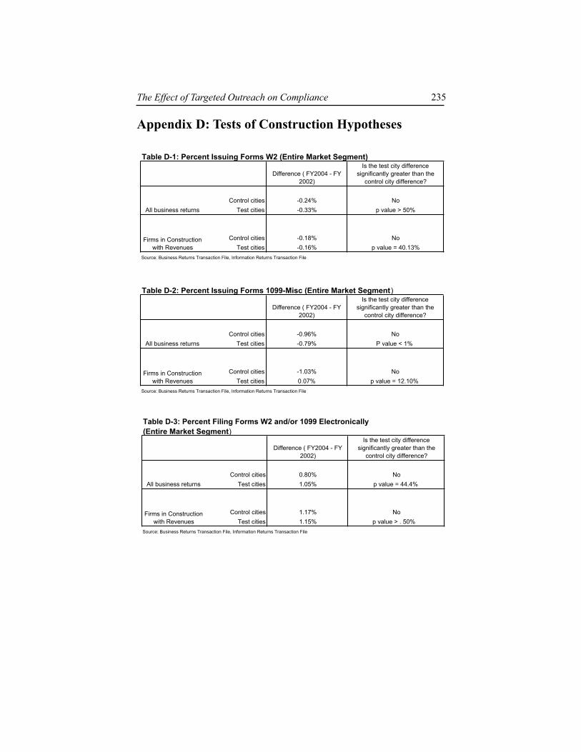
The Effect of Targeted Outreach on Compliance 235
Appendix D: Tests of Construction Hypotheses
Difference ( FY2004 - FY 2002)
Is the test city difference significantly greater than the
control city difference?
Control cities -0.24% NoTest cities -0.33% p value > 50%
Control cities -0.18% NoTest cities -0.16% p value = 40.13%
Table D-1: Percent Issuing Forms W2 (Entire Market Segment)
All business returns
Firms in Construction with Revenues
Source: Business Returns Transaction File, Information Returns Transaction File
Difference ( FY2004 - FY 2002)
Is the test city difference significantly greater than the
control city difference?
Control cities -0.96% NoTest cities -0.79% P value < 1%
Control cities -1.03% NoTest cities 0.07% p value = 12.10%
Table D-2: Percent Issuing Forms 1099-Misc (Entire Market Segment)
All business returns
Firms in Construction with Revenues
Source: Business Returns Transaction File, Information Returns Transaction File
Difference ( FY2004 - FY 2002)
Is the test city difference significantly greater than the
control city difference?
Control cities 0.80% NoTest cities 1.05% p value = 44.4%
Control cities 1.17% NoTest cities 1.15% p value > . 50%
Table D-3: Percent Filing Forms W2 and/or 1099 Electronically(Entire Market Segment)
All business returns
Firms in Construction with Revenues
Source: Business Returns Transaction File, Information Returns Transaction File

Adelsheim and Zanetti236
Difference ( FY2004 - FY 2002)
Is the test city difference significantly greater than the
control city difference?
Control cities -3.69% NoTest cities -2.58% p value = 48.0%
Control cities -0.91% NoTest cities -0.20% p value = 48.8%
Table D-4: Percent Issuing Forms W2 (Panel)
All business returns
Firms in Construction with Revenues
Source: Business Returns Transactions File, Information Returns Transactions File
Difference ( FY2004 - FY 2002)
Is the test city difference significantly greater than the
control city difference?
Control cities -1.05% NoTest cities -2.39% p value > 50%
Control cities -0.91% NoTest cities -0.34% p value = 49.2%
Table D-6 Percent Filing Forms W2 and/or 1099 Electronically (Panel)
All business returns
Firms in Construction with Revenues
Source: Business Returns Transactions File, Information Returns Transactions File
Difference ( FY2004 - FY 2002)
Is the test city difference significantly greater than the
control city difference?
Control cities -3.49% NoTest cities -2.52% p value = 48.8%
Control cities -0.92% NoTest cities -0.28% p value = 47.6%
Table D-5 Percent Issuing Forms 1099-Misc (Panel)
All business returns
Firms in Construction with Revenues
Source: Business Returns Transactions File, Information Returns Transactions File

The Effect of Targeted Outreach on Compliance 237
Did the Firm Issue Forms W2 in
FY2002?% Issuing Forms w2 in
FY2004Are the test cities significantly greater than the control cities?
Control cities 1.01% NoTest cities 0.67% p value > 50%
Control cities 87.95% NoTest cities 87.29% p value > 50%
Control cities 0.31% NoTest cities 0.13% p value > 50%
Control cities 90.55% NoTest cities 85.33% p value > 50%
Table D- 7: Percent Filing Forms W2 by Filing Behavior in FY2002 (Panel)
All business return - No
All business return - Yes
Firms in Construction with Revenues - No
Firms in Construction with Revenues - Yes
Source: Business Returns Transactions File, Information Returns Transactions File
Did the Firm Issue Forms 1099-Misc in
FY2002?% Issuing Forms 1099 in
FY2004Are the test cities significantly greater than the control cities?
Control cities 3.29% NoTest cities 3.26%
Control cities 72.28% YesTest cities 73.58% p value = .0324
Control cities 6.47% NoTest cities 6.28%
Control cities 68.52% NoTest cities 71.44%
Source: Business Returns Transactions File, Information Returns Transactions File
Table D-8: Percent Filing Forms 1099 in FY 2004 by Filing Behavior in FY2002 (Panel)
All business returns - No
All business returns - Yes
Firms in Construction with Revenues - No
Firms in Construction with Revenues - Yes

Adelsheim and Zanetti238
Did the Firm File Electronically in
FY2002?% Filing Electronically in
FY2004Are the test cities significantly greater than the control cities?
Control cities 1.55% NoTest cities 1.21% p value > 50%
Control cities 55.38% NoTest cities 59.33% p value = 26.2%
Control cities 0.96% NoTest cities 1.18% p value = 49.4%
Control cities 72.73% NoTest cities 48.15% p value > 50%
Table D-9: Percent Filing Forms W2 or 1099 Electronically by Filing Behavior in FY2002 (Panel)
All business return - No
All business return - Yes
Firms in Construction with Revenues - No
Firms in Construction with Revenues - Yes
Source: Business Returns Transactions File, Information Returns Transactions File

The Effect of Targeted Outreach on Compliance 239
Tabl
e D
-10:
New
Tax
paye
rs in
the
Con
stru
ctio
n Ex
perim
ent Diff
eren
ce (
FY20
04 -
FY 2
002)
Is th
e te
st c
ity
diffe
renc
e si
gnifi
cant
ly
grea
ter t
han
the
cont
rol c
ity d
iffer
ence
?
0.86
%N
o0.
77%
p va
lue
> 50
%
All
busi
ness
retu
rns
Con
trol c
ities
Yes
Test
citi
es(p
val
ue<
.01)
Con
trol c
ities
No
Test
citi
esp
valu
e >
. 50%
All
busi
ness
retu
rns
Con
trol c
ities
No
Test
citi
esp
valu
e >
50%
Con
trol c
ities
Test
citi
esPerc
ent o
f New
Bus
ines
ses
Issu
ing
Form
s W
2
All
busi
ness
retu
rns
Con
trol c
ities
Test
citi
es
Firm
s in
Con
stru
ctio
n w
ith R
even
ues
Con
trol c
ities
Num
bers
too
smal
l for
ana
lysi
sTe
st c
ities
Perc
ent o
f New
Bus
ines
ses
Issu
ing
Form
s 10
99 -
MIS
C1.
85%
2.05
%
Firm
s in
Con
stru
ctio
n w
ith R
even
ues
3.23
%3.
00%
Sou
rce:
Bus
ines
s R
etur
ns T
rans
actio
ns F
ile, I
nfor
mat
ion
Ret
urns
Tra
nsac
tions
File
% o
f New
Bus
ines
ses
Issu
ing
Form
s W
2 or
109
9_M
ISC
that
file
d th
em e
lect
roni
cally
0.09
%0.
08%
Firm
s in
Con
stru
ctio
n w
ith R
even
ues
Num
bers
too
smal
l for
ana
lysi
s

A New Era of Tax Enforcement: From ‘Big Stick’ to Responsive
RegulationSagit Leviner* **
The operation of the Federal Government is heavily dependent on income taxes; in 2005, about 43 percent of Federal tax revenue in the United States came from individual income taxes and another 13
percent from corporate income taxes.1 This amounts to $927 billion and $278 billion, respectively2 and, compared with Fiscal Year 2004, an increase of 14.6 percent in individual income taxes and 46.9 percent in corporate income taxes.3 Every year, however, the Government collects billions of dollars less in tax money than it believes is owed. This difference between taxes owed and taxes collected--otherwise known as the “tax gap”4--is substantial and has nearly tripled over the past 2 decades.5 Estimates released in February 2006 indicate that the U.S. tax gap for the 2001 tax year stands at approximately $345 billion dollars,6 corresponding to a noncompliance rate of 16.3 percent of taxes owed.7 Both of these numbers fall at the high end of the range of estimates provided by the IRS in the spring of 2005.8 Through enforcement activities and collection of other late payments, the IRS intends to eventually close some of this gap, still leaving an enormous net deficit of approximately $290 billion for the 2001 tax year.9
Noncompliance with the tax law may occur in various ways, including taxpayers’ failure to accurately report their tax bases, to correctly assess tax liability, to timely file tax returns, or to promptly pay taxes due.10 However, more than 80 percent of the tax gap comes from underreporting of taxes--mostly of income tax11--meaning that many taxpayers either provide a partial report of their tax bases or completely fail to acknowledge an existing liability. Noncompliance may not be exclusively intentional and can stem from a wide range of causes, including “lack of knowledge, confusion, [or] poor record keeping.”12 These problems may arise because “the taxpayer is ignorant, lazy, careless…following common practices in occupational groups or workplaces, heeding incorrect advice from the IRS…, taking the advice of a tax professional who recommended strategies that shade into illegality, or many other reasons.”13
Actions that challenge the integrity of the tax system can be categorized into three broad groups. On either end of the spectrum are tax evasion and

Leviner242
tax avoidance, while a third group, aggressive tax planning, is somewhere in between. Despite the fact that evasion and avoidance have much in common in the economic realm, from a legal standpoint, evasion differs significantly from avoidance in that evasion is unlawful and hence subject to legal punishment. Indeed, tax evasion is commonly defined as a deliberate failure to comply with one’s tax obligation in a manner which clearly violates the law.14 This could include, for example, failure to submit tax returns or to report income that is received in cash. In comparison, tax avoidance (also known as “tax reduction”) occurs when the taxpayer intentionally reduces her tax liability in a way that may be unintended by the legislator but is permissible by law.15 Avoidance may be accomplished by constructing business transactions such that tax liability is minimized, often through exhausting favorable tax treatments, including any of the deductions or credits available in the Tax Code.16 The third form of tax noncompliance is a specific--more extreme--type of tax avoidance commonly referred to as “aggressive tax planning” (sometimes known as “abusive tax shelters”). Taxpayers in this group seek to exploit deficiencies or uncertainty in the law in order to comply (only) with the letter of the law while ultimately undermining the policy intent or rationale behind it.17
Maintaining the integrity of the tax system is a difficult task in all societies.18 Tax noncompliance or, at times, creative compliance, furthers a climate of disrespect, antagonism, and selfishness in the relationship among citizens and between them and the Government.19 Moreover, when taxes are compromised, the tax system becomes a deficient means for raising money to pursue and implement Government goals, and actual tax collection fails to reflect the statutorily intended taxation plan.20 This creates disturbing results such as upsetting the distribution of tax burdens and, more generally, wealth in society.21 For instance, when wealthy citizens have better opportunities and means to reduce their tax liabilities compared with other less well-off citizens, the taxes collected are likely to result in a more regressive and less equitable system than the legislative intention.22 Abusive tax practices also jeopardize horizontal equity when there exists an unequal distribution of opportunity to reduce or eliminate tax liability.23 Furthermore, in a country with fixed revenue requirements, reducing the tax liability for any given sector of taxpayers, in effect, means that higher and more distortionary taxes are levied on others.24 All of this, in turn, produces inefficiencies as market competition is affected by the unequal distribution of the tax burden and by economic practices motivated by tax abuse,25 creating a deadweight loss to society.26
Despite the benefits entailed in improving compliance, the complexity of the Tax Code and the magnitude and persistent levels of noncompliance make it so that no tax system can achieve perfect compliance.27 Still, due to the size of the tax gap, even a small or moderate reduction in existing

A New Era of Tax Enforcement 243
noncompliance could yield substantial returns and improve the Government’s ability to pursue its goals. According to a 2004 Government Accountability Office report, each 1 percent reduction in the net tax gap in the United States would likely yield more than $2.5 billion annually.28 Thus, a 10-to 20-/percent reduction of the net tax gap could translate into $25 billion to $50 billion or more in additional revenue annually.29
In recent years, the IRS has taken a number of steps to bolster enforcement and ease the tax gap. The IRS budget request for Fiscal Year 2005 was $10.674 billion, $490 million more than the amount proposed in Fiscal Year 2004.30 Three hundred million dollars of this increase were allocated for enforcement.31 The enforcement budget was used to raise the audits of high-income taxpayers who are earning $100,000 or more to 221,000 reviews in Fiscal Year 2005, the highest number of reviews in the past 10 years.32 Similarly, the number of audits of all taxpayers increased to 1.2 million in 2004, a 20-percent increase from the year before.33 As a result of these steps and others, the IRS reported an increase in its enforcement revenue of nearly 40 percent from a total of $33.8 billion in 2001 to $47.3 billion in 2005.34 Unfortunately, despite these recent increases in enforcement and revenue, the difference between taxes owed and taxes collected remains considerable, begging the question of whether there is something else that can be done to alleviate the problem of tax noncompliance.
This paper suggests that expansion of the traditional tax compliance analysis to include responsive elements of regulation, as illustrated in the Australian approach to tax enforcement, will lead to a more credible, effective, and forward-looking model of tax compliance and enforcement than available under alternative models. Given that responsive regulation was first introduced in the Australian tax administration during the late 1990s and has yet to produce an appreciable amount of verifiable information, compliance improvement data on this approach to tax are currently limited. This paper therefore focuses on fleshing out the underlying principles and rationales of the Australian approach to tax enforcement. In a few years, the Australian model can be evaluated against more comprehensive data and empirical work. In the meantime, interest of countries such as the United Kingdom and Canada in the Australian model and the implementation of this model in New Zealand may indicate that the responsive approach to tax enforcement is more than a passing phase.
The first part of this paper discusses the main reasons tax compliance is a challenge for tax administrations and the manner in which economic analysis can offer important insights into and methodological guidance for understanding noncompliance and improving compliance. The second part reviews the origins of the economic analysis of compliance, explains how the economic model was introduced into the area of tax enforcement, and

Leviner244
explores more recent developments in the economic model. The third part discusses key advantages and disadvantages of the economic approach to tax compliance, concluding that the economic model is persuasive in many respects yet flawed in others. The fourth part introduces the Australian approach to tax enforcement, explaining that this approach draws heavily on the economics of crime and compliance, yet it moves beyond the economic realm to rely on other theories and, as a result, has the potential to capture the strengths of the economic model while also addressing some of its drawbacks. The fifth part summarizes and concludes the paper, suggesting that the Australian approach to tax compliance may mark the beginning of a new era of tax enforcement. The main focus of this paper is personal income tax compliance although much of the discussion can also be applied to other areas of tax compliance. Regrettably, there are many important issues that fall outside the scope of this paper. Most notably, this paper does not examine the literature on the underground economy, or on the difficulties with collecting taxes internationally, nor does it consider the relative advantages and/or disadvantages of sales taxes or Value Added Tax (VAT) compared with income taxation in terms of their ease of enforcement. These issues, although important, are left for future inquiries.
The Problem and Modeling of Tax ComplianceThe difficulties of tax enforcement emerge, to a great extent, because the variables that define the tax base are usually not observable.35 That is, without detailed information about the taxpayer’s various financial transactions and her overall financial (and other tax-related) standing, no one but the taxpayer can know her true tax liability and, therefore, whether she is truthful and accurate in her report to the tax authorities. To a certain degree, verifying information may be obtained by means of costly audits or third-party reporting, such as by banks and employers.36 Assuming that this information can be acquired in a timely and cost-efficient manner and is found to be accurate and coherent, the tax base becomes verifiable.37 In other cases, however, as when the taxpayer is involved in transactions that are beyond the reach of the tax authority and official statistics, including when income is received by way of cash transactions, the tax base is almost impossible to verify.38
The taxpayer is able to use the unobservable nature of the tax base to her advantage or, in other cases, to make innocent mistakes by reporting a partial or otherwise incorrect figure on her tax return in a manner that is difficult to detect. At times, it can also be difficult for the tax administration to clearly

A New Era of Tax Enforcement 245
identify which taxpayer is most likely to be noncompliant. Some of the key influences for whether a taxpayer will comply, such as the perceived probability of detection and opportunities for evasion, can be rather tricky to capture and to compute. All these shortcomings make it extremely complicated to not only detect or correct noncompliant behavior but also to study and better understand its possible causes and facilitators. Amidst these difficulties, economic analysis can intervene and offer methodological guidance.
Over the past three decades, economic analysis of tax compliance has played an important role in elucidating the issue of compliance and, specifically, pinpointing those factors involved in the (lack of) compliance of taxpayers. As compliance issues are examined, analysts simplify the many complexities involved in order to produce a coherent framework that draws attention to the essential questions.39 Modeling tax compliance further facilitates an important process in policymaking: examining and comparing the possible consequences of establishing alternative enforcement strategies.40 This, in turn, allows policymakers to deliberate on and offer various policy alternatives to pursue.
Although valuable information may become available through economic analysis, economic models provide, at best, “a tentative guidance in well-defined circumstances.”41 Models simplify a much more complex reality, making them, almost by definition, unrealistic and, therefore, subject to criticism.42 To a certain extent, improvements in data and in methodology may help bring models closer to real-life scenarios. All models, however, have their shortcomings, and these must be recognized when models are implemented to generate policy recommendations. It is therefore not surprising that researchers generally agree that no one model can offer a complete picture of the tax compliance phenomenon but rather that each may illuminate a certain, or a few, aspects of the problem.43 With these limitations in mind, the next part of this paper will introduce the basic elements of the economic model of compliance with the law.
Originating in the utilitarian paradigm, the economic model of compliance dates back to Jeremy Bentham and Cesare Beccaria and remains very influential to this day. This model suggests that criminal behavior is the result of a rational calculation of the costs and benefits of compliant versus noncompliant behavior, implying that compliance can be improved by policymakers tweaking these costs and benefits such that compliance becomes the beneficial or rational behavior to pursue. After introducing the economic model, the paper will move to explore its application to tax compliance and to discuss some of the later developments and challenges in that area.

Leviner246
Economic Analysis and Tax Enforcement Becker’s Approach to Criminal Law Enforcement and the Deterrence Hypothesis
“The profit of the crime is the force which urges man to delinquency: the pain of the punishment is the force employed to restrain him from it. If the first of these forces be the greater, the crime will be committed; if the second, the crime will not be committed.”44
The principal model for analyzing compliance with the law is drawn from the classic work in utilitarianism by Jeremy Bentham and Cesare Beccaria who laid the foundation for a framework of economic analysis that is relatively simple and that generally fits with human and market behavior in useful ways.45 The basic premise of the utilitarian framework is that people behave rationally in order to maximize their expected utility.46 In the context of compliance, the assumption is that, facing a feasible set of possible courses of action, some of which are legal while others are not, individuals choose whether to commit a crime or not based on whether the one option or the other has the better prospect of increasing their well-being.47 The economic approach to compliance, although influential at the time it was first developed, received very little attention from later theorists and policymakers until it reappeared and was modernized in Gary Becker’s pathbreaking article entitled Crime and Punishment.48
In the decades prior to the publication of Becker’s paper on crime and punishment, discussions of crime were dominated by the opinion that criminal behavior is caused by mental illness and social oppression and that criminals are no more than victims of their life circumstances.49 According to Becker, these attitudes began to have a major influence on social policy, as laws were enacted to expand the rights of those who were lawbreakers.50 Becker not only rejected the presumption that criminals were helpless victims of their situations but also took issue with the associated policy implications, which, according to him, ultimately “reduced the apprehension and conviction of criminals and provided less protection to the law-abiding population.”51 Instead of adhering to theories of mental illness and social oppression, Becker’s analysis explored the possibility that criminal behavior is in fact rational and that it should be handled as such by policymakers.52
In a recent article, Becker explains that he first began to think about crime in the late 1960s after driving to Columbia University for an oral examination of a student in economic theory.53 Becker was late and had to decide quickly whether to take the extra time to put his car in a parking lot or risk getting a ticket for parking illegally on the street.54 Confronted with this dilemma,

A New Era of Tax Enforcement 247
Becker contemplated the faster solution of parking on the street and assessed the likelihood and severity of getting a ticket for violating the city parking regulations.55 Based on this assessment, Becker reached the conclusion that it was worth it to take the risk and park on the street.56 As he was walking away from his car to the examination room, it occurred to Becker that “the city authority had probably gone through a similar analysis”57 and that “the frequency of their inspection of parked vehicles and the size of the penalty imposed on violators should depend on their estimates of the type of [rational] calculations potential violators like me would work.”58
Becker clarifies: “[T]heories about the determinants of the number of offenses differ greatly, from emphasis on skull types and biological inheritance to family upbringing and disenchantment with society. Practically all the diverse theories agree, however, that when other variables are held constant, an increase in a person’s probability of conviction or punishment if convicted would generally decrease, perhaps substantially, perhaps negligibly, the number of offences he commits.”59 Broadly stated, according to Becker, what ultimately governs the decision of individuals whether to commit an offense or not is their reasoned calculations of the costs and benefits they may face by committing a crime as opposed to obeying the law. Since the final consequences of criminal behavior are generally uncertain, Becker employs the common assumption that people act as if they are maximizing their expected utility and that utility is a positive function of income. In Becker’s words: “[A] person commits an offense if the expected utility to him exceeds the utility he could get by using his time and other resources at other activities. Some persons become ‘criminals,’ therefore, not because their basic motivations differ from that of other persons, but because their benefits and costs [resulting from compliance and noncompliance with the law] differ.”60
Focusing on the costs and benefits entailed in human behavior, the “deterrence hypothesis” emerges suggesting that, if individuals are rational decisionmakers whose aim is to maximize their expected utility, then the way for the authorities to ensure compliance with the law is to deter individuals from acts of noncompliance by making the expected utility of noncompliance lower (i.e., less beneficial) compared with the expected utility of compliance.61 In particular, Becker advances the argument that public resources ought to be allocated to policy measures of two kinds: one aimed at detecting noncompliers (i.e., increasing the probability of enforcement) and the other designed to ensure devastating consequences for offenders (i.e., inflicting legal sanctions). He argues that finding the right (optimal) balance between the two measures can effectively deter offenders and make compliance the rational choice for individuals.62

Leviner248
The Allingham-Sandmo Model of Tax EvasionCompared with the general economic theory of crime, its tax noncompliance counterpart is a relatively recent development, dating back to a little over 30 years ago and, particularly, to the much cited article, Income Tax Evasion: A Theoretical Analysis, by Michael Allingham and Agnar Sandmo.63 Allingham and Sandmo extended Gary Becker’s work on the economics of crime to taxation using modern risk theory, and their 1972 publication serves as a cornerstone, leading to a large number of scholarly contributions either commenting or expanding on their insightful essay.64
Like previous research in crime, Allingham and Sandmo build their analysis around the individual, this time the taxpayer, who becomes the potential criminal.65 Their model explores the decision to evade at the moment when the taxpayer is filling in her tax return. The issue of compliance is presented as a portfolio allocation problem in which the taxpayer must decide what portion of her income to allocate to various activities, some of which are legal (i.e., income declared on the tax return), while others are illegal (i.e., income not reported).66 Specifically, the model, which I will call the A-S model or framework, examines the way the decision whether to evade or comply relates to the manner in which the taxpayer perceives her economic opportunities and well-being to be affected by enforcement measures (i.e., audit probability and the severity of sanctions) as well as by the Tax Code (i.e., the tax rate).
Allingham and Sandmo begin their analysis by considering a basic model in which the authorities decide on the Tax Code and the enforcement mechanisms, while each taxpayer acts as if her actions do not influence these decisions.67 The taxpayer is taken to be familiar with the tax legislation, the probability of an audit, the taxes she is liable for, and the penalty for failing to pay that amount in the event that she is caught and convicted.68 Other important simplifications of the analysis include the assumption that the taxpayer is risk-averse,69 that the tax system is income-based, and that the taxpayer’s actual income is exogenously given and is known to the taxpayer but not to the Government’s tax collector.70 Tax is assumed to be levied at a proportional rate on declared income which represents the taxpayer’s decision variable.71 With some constant probability, the taxpayer is subjected to investigation by the tax authority that may then reveal the actual amount of her income.72 If this happens, the taxpayer would have to pay tax on the undeclared income at a penalty rate which is higher than the tax rate.73 Finally, the decision whether to evade or comply is analyzed as if it is the only dilemma with which the taxpayer is concerned,74 and the analysis ignores possible interrelationships between this decision and other economic choices the taxpayer may face including, for example, decisions concerning labor

A New Era of Tax Enforcement 249
supply or tax avoidance (rather than evasion).75 The basic A-S analysis also assumes that time is composed of a single period76 and that only one form of evasion is available.77
Patterned after the utilitarian paradigm, the taxpayer is assumed to follow expected utility theory and to make compliance decisions based solely on the consequences for her net income.78 The A-S framework accordingly implies that the taxpayer is tempted to seize the opportunity of cheating on her taxes whenever it is worth the chance of being caught and bearing the associated penalties.79 The taxpayer is therefore confronted by a classic dilemma of choice under uncertainty or what has also been described as a “lottery calculation” or a “gamble.”80 This lottery calculation, or gamble, requires the rational, utility-maximizing taxpayer to ask herself whether given what she knows about her economic situation, her tax obligation, and the enforcement mechanisms, the likely rewards gained from evasion are worth bearing the risk of being caught and penalized.81 The taxpayer has a choice between two main strategies: She may declare her income in full or she may declare less than that amount, and, in that case, the taxpayer must decide what portion of her income to declare and what portion to conceal.82 If the taxpayer chooses to conceal some (or all) of her income, her payoff will depend not only on her decision regarding whether to evade (and to what extent) but also on whether she is investigated by the tax authorities and becomes subject to some (or all) of the associated penalties.83 To decide which strategy to choose, the taxpayer must compare the expected utility gained from evasion--the taxes she will not pay--with the expected cost of the penalty--the nominal penalty discounted by the probability that this penalty will be imposed.84 If caught, the taxpayer will need to pay not only the penalty for evasion but also the tax shortfall. When the expected value of evasion is positive, the taxpayer will evade, and, when it is negative, she will comply.85
An illustration may be helpful. Consider an example given by John Carroll where a taxpayer contemplates an illegal deduction that reduces the tax she must pay by $100 and where the probability of an audit is estimated to be 5 percent.86 If audited, the taxpayer would have to pay the $100 plus a penalty of 50 percent of the income owed ($50).87 To simplify the example, Carroll ignores interest rates and treats the taxpayer as risk-neutral.88 According to this scenario, the analysis would involve two main alternatives: (1) not taking the deduction, in which case the result is some initial amount of income, W, and (2) taking the deduction. There are two possible outcomes to taking the deduction: (1) W plus $100 if the taxpayer is not audited, and (2) W minus $50 if she is audited.89 The expected utility of being honest is U(W), and the expected utility of cheating is .95[U(W+100)]+.05[U(W-50)].90 As a point of reference for a risk-neutral taxpayer, Carroll conveniently assumes that U(W)=0 and that U(W+X)=X, so that the expected utility of being honest

Leviner250
is 0 compared to 92.5 for cheating (.95*100 – .05*50).91 With the expected utility for cheating significantly higher for noncompliance compared with compliance, Carroll concludes that the taxpayer in this example will cheat.92
Examining the relationship among (1) actual income, (2) the tax rate, (3) the penalty rate, (4) the probability of detection, and (5) tax evasion, the analysis of Allingham and Sandmo leads to results that partly contradict available compliance data in that it suggests that there is no clear relationship among actual income, the tax rate, and evasion.93 However, the results for the penalty rate for evasion and the probability of detection are unambiguous, and the A-S model confirms Becker’s analysis concluding that a higher penalty rate and/or probability of detection tends to discourage tax evasion.94 Allingham and Sandmo clarify that, while the expected tax yield would fall with a decrease in the probability of detection, the loss of tax revenue could be compensated by an increase in penalty rate,95 such that the two enforcement alternatives are substitutes for one another.96
The Economic Analysis of Tax EvasionBeyond the Allingham-Sandmo ModelThe economic approach to tax compliance, as it appears in the A-S framework, reduces enforcement to two key considerations: the penalty rate and the probability of detection. In other words, the A-S analysis suggests that, in order to control evasion, either detection has to be stepped up and/or penalties need to be increased. While this conclusion generally provides an intuitively appealing and straightforward description of the tax evasion phenomena, real-world tax compliance and enforcement are much more complex than this analysis suggests.97 Efforts to add the necessary depth and realism to the study of tax compliance have resulted in the A-S framework being the subject of considerable research over the past three decades. This research has included attempts to endogenize various critical parameters involved in compliance and to incorporate additional and more diverse variables relating to taxpaying behavior.
Early attempts to add credibility to the A-S analysis are evident already in the original 1972 article where Allingham and Sandmo briefly analyze a dynamic case of tax evasion incorporating an element of time.98 These attempts continued with later works of scholars such as Michael Landsberger, Isaac Melijson, Josef Greenberg, Eduardo Engel, and James Hines.99 Advocating a departure from the static framework in which the taxpayer makes only one tax report independent from past or future tax filings, these scholars consider a more general and realistic framework whereby the taxpayer makes a sequence

A New Era of Tax Enforcement 251
of tax filings that become interdependent.100 This modification of the basic A-S model of evasion was necessary, as recognized by Allingham and Sandmo, because, in real life, enforcement decisions are not made independently of one another. For instance, once a taxpayer is discovered to have cheated, the authorities are likely to investigate her honesty for other periods.101 Similarly, because income tax reporting is normally an annual event, it is possible that the taxpayer makes a decision regarding her present and future reports based on what she learns from her past reports and audit experience.102
Another important development in the A-S framework involves efforts to further endogenize the probability of detection. Allingham and Sandmo originally assumed the probability of detection to be exogenous to the taxpayer.103 However, as suggested above, actual audit probability is not random or fixed and generally depends on the particular characteristics of taxpayers. To give one obvious example, in the United States, the IRS developed formulas for selecting returns to audit based on their likelihood to contain suspicious items, and the tax administration also often focuses on the potential to maximize enforcement revenue through audit adjustments.104 For these reasons, audit rates vary across taxpayers. Returns of high-income individuals are generally examined more frequently compared to those with lower incomes, and larger corporations are examined more often than smaller ones.105 Based on the relationship evident in real-world enforcement between taxpayers’ income levels and their audit probability, commentators on the A-S analysis suggested modifying the analysis so that the probability of audit would not be fixed but rather become a function of reported income and evasion.106 The resulting analysis relaxes the unrealistic assumption that taxpayers and the tax administration ignore each other’s actions and treats the interaction between them more as a strategic game--where each party makes the best response to the other’s strategy in light of available information--rather than a static gamble.107
Another variation of the A-S model worth noting incorporates labor-supply decisions as endogenous to the taxpayer’s gross income.108 This type of model recognizes that “it is unreasonable to believe that the taxpayer has not thought about the possibility of evading taxes before he sits down to fill out his income tax return”109 and that “more probably, he has thought about this [matter] before making decisions about the allocation of his work and leisure hours or about the composition of his investment portfolio.”110 Accordingly, models that incorporate labor-supply decisions look beyond the fairly simple A-S framework which offers only two behavioral responses on the part of the taxpayer--evasion or compliance--and consider that the taxpayer may respond to taxation in other ways. These responses generally include changing work effort, altering decisions about consumption and savings, and choosing legal (compared to illegal) tax reduction strategies.111 Models in this group usually

Leviner252
focus on how variables such as the tax and wage rates affect the taxpayer’s responses and the manner in which any one response affect the others.112
Unfortunately, although this type of model adds realism to the analysis of tax compliance, incorporating labor supply considerations make uncertain the effect of changing the enforcement variables, thus eliminating the relatively simple computations of the original A-S framework such that “depending on the taxpayer’s marginal disutility from labor and her risk attitudes, all predictions become possible.”113
In an effort to obtain a more thorough understanding of tax compliance, researchers continue to develop more credible models of tax compliance that, among other things, introduce complex forms of evasion; include detailed tax penalty structures; account for imperfect information and randomness in the audit rate and in taxpayers’ true tax liabilities; examine the role tax practitioners play in compliance; extend the number of items on which taxpayers report; and also address the possible impact of tax morale, justice, and fairness considerations on tax compliance. Although the traditional economic analysis of tax compliance has been expanded to include these and other more detailed and realistic explanatory variables, its focus on only two key enforcement tools, punishment and detection, remains unsatisfactory and does not reflect real-world enforcement practices or needs. Furthermore, the underlying assumption of the economics of compliance--that every person is engaged in some type of rational calculation where the taxpayer conceals income as long as the return on noncompliance is positive--does not always coincide with taxpaying behavior.114 According to survey information, the majority of people consider themselves to be honest in their tax reporting,115 and presumably they are, if the estimated noncompliance rate of 16.3 percent is accurate.116 In fact, it has repeatedly been suggested in tax compliance literature that “given the current mild sanctions and low probability of detection … [one] would predict that virtually everyone should be evading tax.” In other words, instead of asking “Why do people evade taxes?” we should be asking, “Why do people pay them?.”117 The next section of the paper will explore the strengths and shortcomings of the economics of crime view of compliance, especially as it relates to enforcement, and will make a case for taking the necessary steps toward developing a more comprehensive interpretation of taxpaying behavior in order to better understand tax compliance and address noncompliance.

A New Era of Tax Enforcement 253
An Expanded View of Taxpaying Behavior A Look at Enforcement Strategies: Deterrence and General Prevention “If we put more police into a neighborhood, we are just as likely to
increase the crime rate as to reduce it. The reason is that … police do a lot of things that make crime worse (as well as a lot that makes it better).”118
As evident from the above discussion, to a considerable degree, the standard analysis of tax compliance continues to rely on conventional modern economic theory that views tax evasion as a special case of crime.119 According to this line of thinking, tax noncompliance is the result of a careful calculation in which the taxpayer chooses to cheat on her taxes when that course of behavior best satisfies her preferences (i.e., maximizes her expected utility or favorability of outcomes). This analysis generally presumes that the taxpayer is rational, pursues her self-interest, and possesses the same structure of stable preferences as other taxpayers represented by an expected utility function. Utility is assumed to increase with an increase in disposable income but at a decreasing rate. Working from these assumptions, it becomes relatively easy to test the effect of changing variables in the economic framework, particularly whether a change in enforcement efforts affects the level and extent of noncompliance with the tax law.
Empirical and experimental studies tend to support the economic model of compliance to the extent that they generally indicate a negative relationship between the probability and severity of punishment and the rate of crime. In other words, an increase in either the probability or the severity of punishment can change the expected utility of noncompliance from positive to negative, thereby deterring potential offenders and, overall, decreasing the level of crime.120 This effect has also been identified in the area of tax compliance.121 The correlation between increased enforcement and compliance appears to be stronger when the probability of punishment is increased than when the punishment is more severe. In either case, however, enforcement efforts relying only on punitive strategies do not always alleviate the problem of noncompliance and, at times, might even worsen the situation.
More specifically, data on tax enforcement generally support the conclusion that taxpayers are responsive to perceived or actual risk of detection in their compliance decisions. According to the IRS’s estimations, compliance is most likely where the risk of detection is significant, such as when there is third-party reporting or withholding. Approximately 1 percent of all wage, salary, and tip income is misreported, contributing about $10 billion to the tax gap.122 In contrast, nonfarm sole proprietor income, which is subject to

Leviner254
little third-party reporting or withholding, has a significantly higher rate of misreporting at approximately 57 percent, which contributes about $68 billion to the tax gap.123 In terms of the punishment parameter, fines and other types of penalties also generally improve compliance. Studies, however, indicate that, when it comes to real-life behavior, small changes in penalties are easily overlooked and unlikely to affect compliance.124 Some researchers go as far as to argue that heavy penalties do not always produce more compliance compared to lighter ones, especially when detection probability is high.125 In certain studies, the effect of an increase in the severity of punishment was not statistically significant, and a statistically significant positive effect on criminal behavior was also occasionally identified.126 Ultimately, it is generally the case that penalties serve as less of a deterrent for committing crimes than the probability of detection.127 Edward Cheng summarizes this point nicely, reporting that the effect of deterrence decreases rapidly (and nonlinearly) with lower probabilities of enforcement, and tougher punishments are often unable to offset these losses.128
Despite the heightened deterrent effect achieved through detection compared with punishment, a concern for low-cost tax administration may lead policymakers to favor raising penalties over increasing costly detection in order to improve compliance. In other words, given a fixed enforcement budget, efforts to maximize deterrence and raise the most revenue at minimal cost might dictate extreme but rare punishments.129 One might especially endorse fines and monetary sanctions rather than other more resource-intensive forms of punishment, such as imprisonment and probation.130 Unfortunately, however, an enforcement strategy of extreme and rare penalties may be a poor strategic choice because of the repercussions it will have outside of its ability to achieve compliance. For example, rare and extreme punishments can provoke community outrage. The idea that the Government doles out just punishment is undermined when extreme sanctions are disproportionably imposed on lesser offenses.131 Even when it comes to serious crimes, inflicting heavy penalties on a rare few is arbitrary, draconic, and highly discriminatory, especially when many individuals are undertaking similar acts of noncompliance but only a few are caught and punished.132 Such an approach may lead to underenforcement as tax administrators become conflicted between their legal obligations and moral judgments.133 Imposing rare but severe sanctions may also lead to an increase in the severity of crimes committed as offenders realize that the sanctions imposed will be extreme regardless of the actual offence committed and attempt to maximize their gains from crime.134 With extreme consequences for noncompliance, erroneous penalties and the punishment of those who violate the law because of ignorance or honest mistake also become particularly disturbing.

A New Era of Tax Enforcement 255
To be sure, taking any form of punitive enforcement to an extreme threatens the democratic nature of society and carries a risk of inflaming a broader conflict between citizens and the Government. Such an approach to tax enforcement can ultimately backlash by creating what Bruno Frey describes as a “crowding out effect” of whatever intrinsic motivations taxpayers have to comply and setting the tone for a taxpayer-tax authority relationship that is dominated by feelings of antagonism and distrust.135 Ultimately, this type of interaction is likely to diminish taxpayers’ willingness to comply with their tax obligations and might also lead them to actively resist paying their taxes, either legally or illegally.136 From an economic perspective, even where an increase in enforcement is feasible, conducive to democracy, and results in an increase in compliance, it might still not be optimal to raise these efforts to the maximum.137 Enforcement expenditures are a real cost to the economy, while the revenue collected can be viewed as a mere transfer from the private to the public sector.138 Furthermore, increased enforcement of the tax system can also have disincentive effects similar to an increase in tax rates and base and should thus be handled with caution and restraint.139
In addition to the considerations that counsel against extreme enforcement measures, empirical evidence suggests that moderate means of enforcement may also fail to promote compliance. When researchers tested the rate and probability of punishment at moderate (compared to extreme) levels--consistent with those observed in actual tax enforcement practices--the deterrent effect was found to be quite small.140 Taken as a whole, the findings suggest that a broad enforcement approach, where detection and punishment are complementary strategies (rather than extreme substitutions) for one another and, more importantly, where nonpunitive enforcement mechanisms are also considered, might be a superior alternative to relying only on authoritarian deterrence.
In fact, enforcement efforts that rely exclusively on punitive measures and the severity and probability of punishment are likely to be short-sighted at best and counterproductive at worst. In the area of tax, such attempts at shaping behavior often lead to “…a never ending process since each piece of legislation brings new opportunities for avoidance.”141 As John Carroll observed: People adapt, take up new strategies of noncompliance, and become increasingly sophisticated in their risk assessment of getting caught and penalized for wrongdoing.142 A broader, more constructive definition of deterrence than the one adopted by the traditional economic analysis of tax compliance should look beyond the use of threat and legal authority to encompass “any factor that exerts a preventive force against crime.”143 This “general prevention” approach has been understood in the literature of crime to take into consideration not only the direct monetary costs and benefits of compliant and noncompliant behavior but also the external conditions that

Leviner256
affect the fostering of law-abiding norms and morals.144 Such an expansive characterization of deterrence would seek to improve tax compliance not only by means of curbing illegal activity but also by encouraging legal behavior, such as by balancing authoritarian deterrence with positive encouragement and assistance. This balanced approach is a familiar practice in regulatory programs generally and it is considered a particularly appropriate technique in areas where, like taxation, compliance is difficult and is not always in the short-term self-interest of the regulated and where the detection of noncompliance is challenging as well.145
The economic analysis of tax compliance has just recently begun to explore the practical needs and constraints of real-life tax enforcement, and it has more to do in order to stay aligned with the developments in the regulatory literature. If we wish to take the study and enforcement of tax compliance to the next level, it may be time for further research and modeling efforts. This could be done, first and foremost, by developing a broader, more detailed understanding of the many aspects of taxpaying behavior and the manner in which these may correspond with the idea of general prevention. This deeper understanding can then be incorporated into a more inclusive and realistic theory of tax compliance and enforcement than presently available under the economics of crime and compliance.
The Multiplicity of Taxpaying Behavior“Common sense and everyday observations tell us that people refrain from tax evasion--as well as from speeding, shoplifting, and polluting the environment--not only because of their estimates of the expected penalty, but for reasons that have to do with social and moral considerations.”146
The analysis of compliance that is patterned after the economics of crime theory provides an important starting point for thinking about tax compliance. However, although there is evidence to support this framework, it nonetheless represents only one piece of the tax compliance phenomenon. The focus of the economics of crime theory has traditionally been on the effect of enforcement variables on the actions of individual actors, and, especially, on illegal behavior (i.e., evasion compared with avoidance or aggressive tax planning). This analysis emphasizes deterrence and the severity and certainty of punishment as the most important aspects of achieving compliance. It therefore interprets the causes for compliant and noncompliant behavior very narrowly. Behavior, however, is multifaceted and is influenced by many different factors, including taxpayer disposition toward public institutions, ethics, morals, norms, and the perceived fairness of the tax system.147 Moreover, enforcement policies

A New Era of Tax Enforcement 257
themselves are more complex than any combination of penalties and audit probabilities. Institutional and procedural factors, such as tax administrators, tax courts, and tax advisors, as well as the manner in which these bodies interact with the taxpaying community, affect the behavior of the taxpayer.148 The standard economic analysis does not normally account for the effect of these various determinants of compliance. However, increasingly, scholars have been collecting empirical evidence about the role of nonmonetary parameters in impacting taxpaying behavior generally and in improving tax compliance and constraining noncompliance, in particular. At the same time, there have been growing attempts to incorporate these parameters into the more formal economic analysis.
The traditional economic literature on tax compliance examines taxpaying behavior through the decisions of a single individual.149 Set in this way, the analysis fails to put the issue of tax compliance in its broader social setting and, consequently, misses important explanatory opportunities.150 One example of this oversight is the limited range of goods examined in the standard analysis, which tends to portray individuals as concerned only with their private consumption while displaying total disregard for public goods and services.151 Evidence, however, shows that taxpaying behavior depends not only on private consumption capacity but also on what taxpayers believe they obtain from public goods and services. Taxpayers expect to receive some return on the taxes they pay, and, not only do they care about these returns, but they also evaluate whether the tradeoff is equitable compared to what other taxpayers appear to receive.152 James Alm, Betty Jackson, and Michael McKee, for example, find a greater willingness to comply with the tax law among taxpayers who believe that they benefit from public goods.153 Michael Spicer and Lee Becker find that individuals who are told their taxes are heavier than others, evade by relatively high amounts, while those who are told their taxes are lower than others, evade by relatively small amounts.154
One study that compared the impact of various information sources on taxpayers found that social influence and, specifically, perceived attitudes toward noncompliance of those people with whom taxpayers discuss taxes had the strongest impact on taxpayers’ commitment to comply with their tax obligations.155 That is, taxpayers’ commitment to paying taxes is affected not only by what they believe they receive for paying taxes and by their relative gain or loss in consumption compared to that of others, but it may mostly rely on social interaction and the extent to which noncompliance is perceived to be prevalent in the taxpayers’ social environment. When taxpayers believe that people around them generally cheat, they are more likely to cheat themselves, and, when taxpayers believe others are generally honest, they are more willing to pay their own taxes honestly.156 As explained by James Andreoni, Brian Erard, and Jonathan Feinstein, when taxpayers notice that others disregard

Leviner258
statutory taxes, creating an unjust disparity in the allocation of the tax burden or leading to a reduction in the quality or quantity of public goods and services, they may rationalize resisting payment of their own taxes.157 It becomes clear, therefore, that taxpaying behavior is not only the result of isolated calculations of the immediate monetary costs and benefits the taxpayer may incur from compliance versus noncompliance. Taxpaying behavior is also a social process where information, experience, attitudes, and patterns of behavior are shared among taxpayers, impacting their assessments of costs and benefits and, consequently, their actual compliance with the tax law.
Some scholars have gone as far as to argue that moral, ethical, and social factors play a role in compliance that may be more important than the threat of legal punishment.158 Harold Grasmick and Scott Wilbur find, for example, that, while the relationship between the threat of legal punishment and intention to evade taxes is statistically significant, anticipated feelings of guilt and social stigma attached to tax evasion are more strongly associated with deterrence.159 Similarly, Laurie Mason and Robert Mason argue that an appeal to taxpayer conscience or civic virtue can improve tax compliance more than the threat of sanctions.160 Other scholars, such as Marsha Blumental, Charles Christian, Joel Slemrod, and Leandra Lederman, clarify that detection and punishment could be complementary strategies to moral, ethical, and social appeals, especially if they are applied to different groups of taxpayers.161 Regardless of the weight placed on particular enforcement considerations, incorporating nonmonetary parameters and influencers into the traditional economic analysis of tax compliance often results in a better description of real-world taxpaying behavior than a theory built only on selfish monetary assumptions.162 Staying within the economic paradigm, the rationality proposition no longer implies narrow materialism or pure self-interest. Instead, rationality now reflects the reality that most people are constrained by a range of considerations and that these considerations lead them to obey the law when the sum of all potential costs of noncompliance, including likely moral, ethical, and/or social sanctions, outweigh the expected gain.163
In sum, although the standard economic approach to compliance serves as a useful starting point for understanding taxpaying behavior, the narrowness of this framework is restrictive and may lead policymakers to reach misguided conclusions that require enforcement that is too punitive and that might ultimately be counterproductive. When it comes to the behavior of the taxpayer, motives other than the desire to increase one’s net income must be considered. Extending the analysis of tax compliance requires continuing efforts to gain a better understanding of the many influencers on taxpaying behavior and the manner in which enforcement efforts can properly and effectively address them. This process mandates incorporating into the

A New Era of Tax Enforcement 259
theory of tax compliance a much richer category of influencers than currently available and, accordingly, reassessing the role that enforcement policy should play in compliance. It is in this particular line of investigation that researchers in Australia have been involved during the past decade, with results that have important implications for the enforcement of tax compliance in Australia, as well as in other industrialized countries, including the United States. The next portion of the paper will review the research in motivations and, particularly, those motivational influencers that have been identified as commonly associated with taxpaying behavior. The paper will then introduce the concept of responsive regulation and explore the manner in which this approach to regulation may be utilized to bring key elements of tax enforcement together and effectively foster tax compliance.
The Australian Approach to Tax EnforcementMotivational Postures: Attitudes, Behavior, and Service
“Regulating people through understanding the simultaneous emergence and retreat of various postures means that, at the most fundamental level, regulation rests on the art of managing relationships.”164
Innovative research in regulation has identified a group of motivational influencers--best known today as “motivational postures”--that capture the way regulated entities position and think about themselves in relation to the regulatory authority.165 The basic principle behind the concept of motivational postures is that the beliefs, values, and attitudes of regulated actors lead them to adopt a particular posture (or stance) toward the regulator.166 In the context of compliance with tax law, motivational postures capture the manner in which taxpayers see themselves as they relate to the tax system and administration and, particularly, the amount of (social) distance they wish to place between themselves and the latter two.167 This distance indicates the taxpayers’ degree of acceptance or rejection of the tax authority and, accordingly, the extent to which these taxpayers are open to the authority’s influence.168
Strategies for inducing compliance are likely to vary in their effectiveness depending on the motivational posture of the targeted taxpayers. In other words, different regulatory and enforcement measures can be successful when dealing with taxpayers who see themselves as law-abiding citizens versus with taxpayers who see themselves as opportunistic. Moreover, taxpayers who feel insulted or treated disrespectfully by the tax authority may respond better to particular enforcement mechanisms than taxpayers who feel that they have been treated with dignity by an authority that acts with integrity

Leviner260
and legitimacy.169 For this reason, tax administrations that seek to understand taxpayers’ full range of motivational influencers may be better situated to effectively target and encourage taxpayers to “do the right thing” and comply with their tax obligations while, at the same time, monitor and constrain those motivations that may lead taxpayers to noncompliance.170
The business, industry, sociological, economic, and psychological (BISEP) characteristics of taxpayers shed important light on the reasons that taxpayers hold the motivational postures they do and the possible causes for their compliant or noncompliant behavior including (but not limited to) issues of opportunity, ignorance, business norms, and compliance costs.171 By continually exploring the BISEP characteristics through empirical and experimental work and outreach to the taxpaying community, the tax authority can gain insight into how to improve tax compliance in a well-informed and comprehensive manner.172 Ongoing consideration of taxpayers’ BISEP characteristics may also enhance the tax administration’s understanding of the structural and environmental facilitators of noncompliance, and this increased understanding should allow tax administrators to deal with issues of noncompliance at the source. In other words, by investigating taxpayers’ BISEP characteristics, the tax administration may obtain the knowledge necessary to tailor enforcement and regulation to meet particular compliance needs (in some cases) even before taxpayer defiance actually occurs.173 This, in turn, can lead to the development of more effective enforcement strategies in the long run.
Five key motivational postures have been identified as relevant to the realm of tax compliance. They are: (a) commitment, (b) capitulation, (c) resistance, (d) disengagement, and (e) game playing.174 The first two postures, commitment and capitulation, are compliant in nature, the former more than the latter. They suggest cooperative interaction with and acceptance of the tax system and authority by the taxpayer.175 The latter three postures, resistance, disengagement, and game playing, represent an increasingly defiant state of mind with growing distance and dislike on the part of the taxpayer toward the tax authority, system of taxation, and what the taxpayer perceives they stand for.176
When commitment and capitulation are high, the tax administration is more likely to gain taxpayer compliance. The posture of commitment expresses the taxpayer’s understanding that the tax administration is a necessary institution for democracy and suggests a feeling of moral obligation to advance the common good and pay one’s taxes voluntarily.177 Capitulation reflects acceptance of the tax authority and its officials as legitimate and the belief that they are positively responsive to the taxpayer as long as the taxpayer behaves according to the law and obeys the authorities.178 However, when

A New Era of Tax Enforcement 261
the defiant postures of resistance, disengagement, and game playing are high, things are rather different. As eloquently explained by Valerie Braithwaite, a leading scholar in the field of motivational postures, defiant postures are likely to coincide with feelings of being threatened by the tax system or administration, low satisfaction with democracy, antigovernment and pro market attitudes, relatively weak identification with being a citizen and an honest taxpayer, higher than average investment in aggressive tax planning, and a desire to abolish the tax system.179 The defiant postures are also more likely to be unaffected by persuasion, as well as by the traditional punitive measures of being caught and punished for noncompliance.180
Resistance, which is the first posture categorized as defiant, reflects doubts about the intentions of the tax office to cooperate with and be respectful of the taxpayer.181 It represents a state of mind in which the taxpayer is watchful and may feel the need to fight for her rights or to curb the power of the tax authority.182 The second defiant posture, disengagement, is an even more extreme attitude in that it results from a deep disenchantment with the tax system and the tax office.183 The disengaged taxpayer does not see a point in challenging the tax authority, which leaves withdrawal from any interaction with the administration as her main objective.184 Research indicates that disengagement is generally the posture most difficult for authorities to manage.185 As demonstrated in the work of Valerie Braithwaite, John Braithwaite, Diane Gobson, and Tom Makkai on compliance in nursing homes, by mentally positioning themselves outside the regulatory reach, the disengaged can cut themselves off from attempts at persuasion and influence.186 For similar reasons, disengaged taxpayers make it extremely difficult for the tax administration to gain compliance.187 The third and final defiant posture is game playing. With a game playing posture, the taxpayer views the law as something to be respected or ignored based on what advances her interests.188 Unlike disengagement, game playing takes place within the reach of the regulatory authority, but rather than comply with the spirit of the law, the player uses the letter of the law to undermine the law’s intention.189 This posture has traditionally been pervasive in elite groups.190 However, as aggressive tax avoidance strategies become increasingly available to and acceptable by the general public, the game playing mindset is expected to spread and to become a more serious problem for enforcement.191 This posture is a reminder that compliance itself could become a major problem when it is defined as compliance with rules as written.192 In an area as dynamic, complex, and fundamental to society as taxation, the goal for tax enforcement might be better defined as securing long-term compliance with the intent--rather than with the black letter--of the law.193

Leviner262
The more committed people are to paying taxes, the less likely they are to put effort into tax avoidance strategies.194 The postures that have been found to be most strongly associated with aggressive forms of tax avoidance are game-playing and resistance, while evasion has been found to be a more likely option for those who are resistant or disengaged.195 However, being committed or capitulated does not necessarily prevent taxpayers from misconduct.196 Behavior is the result of a variety of inputs, only some of which are related to beliefs and attitudes, and so, consistency between taxpayers’ mental states and behavior should not automatically be assumed.197 The tax administration must acknowledge the disparity between motivational postures and behavior and be cognizant and responsive to both in order to effectively manage compliance. Crucially, the administration does not only serve as a passive observer of the behavior and attitudes of taxpayers, but it also affects them considerably.
In keeping with the influential work in compliance and procedural justice of Tom Tyler, Allan Lind, and others, it is well understood today that the perceptions taxpayers have of the procedural justice of the tax system--how the tax administration treats them and other similarly situated taxpayers--affect the legitimacy taxpayers attribute to the administration and the extent to which they accept its authority.198 This, in turn, impacts taxpayers’ levels of compliance. Taxpayers who believe that the tax administration and its officials make an effort to be fair and respectful are more likely than those with more negative perceptions to assign greater legitimacy to the tax system and administration, align with the administration, and, consequently, be more compliant with their tax obligations.199 In addition, according to the reciprocity rule or norm, positive behavior by the tax administration increases the likelihood of compliance because of the tendency for people to try to treat others in the same manner others treat them.200 Helpful and respectful service may also, therefore, coax a broader normative commitment of compliance among taxpayers when taxpayers believe that the tax administration acts positively toward them as a general (ongoing) practice.201
The result of taxpayer/tax-authority interaction may be different, however, for taxpayers who do not trust or respect the tax authority or for those who feel deeply threatened by it.202 When the taxpayer feels uneasy with the tax authority, such as when the taxpayer anticipates or experiences an unpleasant interaction with tax officials or when she perceives that her self-interested goals are undermined by the administration or the rules it imposes, this taxpayer might adopt a coping mechanism to protect herself against the tax administration’s disapproval.203 This coping mechanism often includes

A New Era of Tax Enforcement 263
interpreting the differences between the taxpayer and the administration as conflicts between “I” (or “us” when the taxpayer identifies herself as part of a group) and “them” (i.e., the tax authority and/or the government).204 To sustain this defensive response, the rift (social distance) between the tax administration and the taxpayer must grow.205 Under these circumstances, gaining compliance from the taxpayer can be difficult. When the tax administration employs punitive strategies that communicate disapproval, the distance and tension between the taxpayer and the administration are likely to increase with the rise in perceived disapproval, reinforcing and exacerbating any existing state of taxpayer defiance.206 The challenge for tax officials in this situation revolves around changing the motivational posture held by the taxpayer.207 Tax officials may be able do this by offering the taxpayer cooperation, positive and helpful service, and open dialogue as a first response to conflicts.208 Importantly, when the offer of cooperation from the tax administration is met with compliance by the taxpayer, toxic feelings such as antagonism, resentment, and distrust between the two can be diffused, such that the ability of the tax authority to (re)connect with the taxpayer on a positive level, and to eventually elicit voluntary compliance, may be restored.209
In cases where the offer of cooperation from the tax administration is not met with compliance by the taxpayer, the tax administration must be firm, but also fair, in bringing to account those who are not compliant. Whatever steps the tax administration takes must not, as much as possible, adversely affect compliant taxpayers or escalate existing conflicts beyond what is necessary in order to gain compliance.210 Maintaining open communication and positive and professional service, even through the toughest encounters with taxpayers, is important for the tax authority not only to preserve its integrity in the eyes of the defiant taxpayer and the broader taxpaying community but also because, in most cases, even when resentment, anger, and disobedience are present on the part of the taxpayer, there is also goodwill and, therefore, an opportunity to draw out the more cooperative motivational postures.211 The question therefore is not whether the tax authority should punish taxpayers who are noncompliant but how the tax authority should do so in a manner that prevents the emergence of widespread taxpayer resistance and fosters goodwill and cooperation.212 The next portion of the paper will draw on the Australian experience beginning in the late 1990s to suggest that an effective approach to achieving taxpayer compliance, mutual respect, and cooperation includes employing a hierarchy of lesser sanctions and regulatory interventions, the possibility of severe and certain sanctions for noncompliance, and the development of a broad understanding of taxpayers’ motivational postures and BISEP profiles.

Leviner264
Responsive Regulation and the Australian Compliance Pyramid
“Through incentives and threats and public statements of what the community considers proper and improper, the law is used as an instrument to shape and maintain behavior.” 213 “The model of the regulatory pyramid suggests regulatory strategies, while the social rift model describes the posturing of those subject to regulation. The ATO Compliance Model brings these different sides of the regulatory relationship together to summarize the process of conflict escalation, not with the intention of avoiding conflict so much as managing it.”214
Until the mid-1990s, the regulatory style of the Australian Tax Office (ATO), like the regulatory approach of most tax administrations in the industrial world, was authoritarian.215 This regulatory method, commonly referred to as “enforced compliance” or “command and control regulation,” developed out of the economics of crime and compliance paradigm. It called for the establishment of clear-cut rules for taxpayers to follow and the enforcement of these rules through threat of detection and legal punishment.216 Despite its widespread dominance, opponents of command and control often argued that this strategy misinterprets human behavior and the meaning of noncompliance and that its one-solution-fits-all approach is poorly suited for regulating compliance.217 The many complexities of the tax compliance problem suggest the need for a comprehensive strategy of enforcement that fosters long-term compliance. Yet “an approach which relies heavily on detecting noncompliance and imposing sanctions on identified offenders tends to be short-term in its effect and increasingly resource-intensive.”218 Eventually, criticisms of the command and control method were taken to heart by the Australian tax administration where, starting with the release of the 1998 Cash Economy Task Force Report,219 a new regulatory approach was taking form--one that moved from authoritarian deterrence to a method of “responsive regulation.”220
In their 1992 book entitled Responsive Regulation: Transcending the Deregulation Debate, Ian Ayres and John Braithwaite conceptualize responsive regulation as a form of regulation that is “responsive to industry structure in that different structures are subject to different degrees and forms of regulation.”221 Responsive regulation is not “a clearly defined program or a set of perceptions concerning the best way to regulate”222 but rather a method that advances the proposition that regulation should be context-dependent.223 In other words, “[f]or the responsive regulator, there are no optimal or best regulatory solutions, just solutions that respond better than others to the plural

A New Era of Tax Enforcement 265
THE AUSTRALIAN COMPLIANCE PYRAMID
Source: Adapted from the 1998 Australian Cash Economy Tax Force Report
MAKE IT EASY
Education/ Record Keeping/ Service Delivery
HELP TO COMPLY
Real Time Examinations/ Record Keeping Review
DETER BY DETECTION
Audit with/ without
penalty
DisengagementCommand Regulation Nondiscretionary
FULL FORCE OF THE LAW
Prosecution & Incapacitation
Commitment
Capitulation
Resistance
Game Playing
MOTIVATIONAL POSTURES
ENFORCEMENT STRATEGIES
REGULATORY STRATEGIES
SelfRegulation
Enforced Self Regulation
Command Regulation Discretionary
configurations of support and opposition that exist at a particular moment in history.”224 An administration that adopts responsive regulation commits itself to investigating and taking into consideration the problems, motivations, and circumstances of the regulated parties. It is an administration that emphasizes dynamic operation, is committed to assisting the regulated actors in their particular compliance efforts, and strives to enforce compliance across the board, even when the regulated are highly resistant.225 At the same time, there is less reliance on strategies that are based only on threat of detection and legal penalties.226
Ayres and Braithwaite utilized the principles of responsive regulation to construct a holistic model for regulating compliance.227 An expanded version of their model was endorsed in the 1998 report of the Australian Cash Economy Tax Force, after which it was adopted across the board for regulating tax compliance in Australia.228 The Australian compliance model is represented graphically by a pyramid with each of its three faces addressing one key aspect of compliance.229 The three faces of the model are: (1) the range of

Leviner266
motivational postures taxpayers are most likely to display in their interactions with the tax administration;230 (2) the range of enforcement strategies available to the tax administration; and (3) the range of corresponding regulatory tools.231 In this model, the motivational postures, regulatory measures, and enforcement strategies have a range of severity. The cooperative postures, lenient enforcement strategies, and less intrusive regulatory styles are set closer to the bottom of the pyramid, while the areas higher on the model are reserved for defiant taxpayers and for harsher, more punitive and authoritarian enforcement and regulatory practices.232
Ayres and Braithwaite introduced the strategy of tit-for-tat (TFT) into the compliance model as a means by which the administration can responsively manage the interaction with the taxpayer.233 In adopting the TFT approach, the Australian compliance model rejects a passive deterrence style where enforcement is grounded in a static calculation of the probability of compliance based on the expected size and risk of punishment.234 Instead, TFT prescribes that the tax administration balance positive persuasion and encouragement with punitive deterrence and incapacitation in a dynamic fashion. The Australian approach, modeled after the TFT strategy, embraces the understanding that people care about different things in different contexts and that they often possess multiple and contradictory selves.235 Most people have a caring, socially responsible self as well as an opportunistic self; they may be motivated by money considerations at one point and by a sense of social responsibility at another.236 Accordingly, an enforcement strategy based only on punishment or persuasion will ultimately fail. Ayres and Braithwaite eloquently explain: “People will exploit a strategy of persuasion and self-regulation when they are motivated by economic rationality. But a strategy based mostly on punishment will undermine the goodwill of actors when they are motivated by a sense of responsibility.”237 Both persuasion and punishment have strengths and shortcomings in delivering compliance, and the key to successful regulation is not to decide between one approach or the other but to establish a workable compromise between the two such that these strategies complement each other.238
When utilizing the TFT methodology, the tax administration balances encouragement and persuasion with punitive deterrence through three stages of communication with the taxpayer: cooperation, toughness, and forgiveness.239 At the heart of this approach is the understanding that the tax office and the taxpayer are interrelated such that they impact and affect one another.240 Accordingly, the TFT strategy commands, among other things, that there be an open communication channel between the tax authority and the taxpayer in which the tax authority explains the legal obligations of the taxpayer and the consequences for noncompliance, and that the imposition

A New Era of Tax Enforcement 267
of these consequences depends on the behavior of the taxpayer.241 The tax administration always starts at the bottom of the compliance pyramid by persuading and encouraging the taxpayer to cooperate.242 If the taxpayer chooses to cooperate, tax officials must respond with cooperation.243 If the taxpayer decides not to cooperate, the compliance pyramid instructs the tax administration to gradually move to a higher level of enforcement and regulation.244 In other words, as conflicts between the tax office and the taxpayer emerge and escalate, the communication between them moves up the pyramid to a higher level of severity, mandating a transfer of power from the taxpayer to the tax office. As the tax authority reverts to a more authoritarian approach of command and control, the taxpayer looses her ability to affect the interaction with the tax office.245 However, the TFT strategy, by being both tough and forgiving, allows the tax administration to not only escalate enforcement and regulation in response--and in proportion--to taxpayer defiance but also to dynamically manage the relationship and conflict with the taxpayer in that it leaves the option of cooperation always within reach.246 As soon as the taxpayer chooses cooperation, the TFT strategy instructs the tax administration to “reward” cooperative behavior by responding with a gradual move down the pyramid and with de-escalation of enforcement and regulation.247
Crucially, with persuasion and encouragement at the bottom of the compliance pyramid, the tax administration must first appeal to the social responsibility of the taxpayer in order to foster compliance. In this way, the administration aims to cultivate relationships of trust and alliance, while avoiding the use of unnecessary punitive measures that might undermine the goodwill and intrinsic motivations of taxpayers to comply.248 By emphasizing measures such as education, good service delivery, and an open dialogue, the tax administration targets the taxpayer’s sense of social responsibility and seeks to bolster the prevention of noncompliance in the enforcement process, taking first steps towards establishing broad political and social support for voluntary compliance as a mainstream option.249 At the same time, by getting tough with cheaters, the tax administration taps into the economics of crime and compliance in that it encourages the taxpayer to choose her socially responsible, law-abiding selves over her opportunistic selves, increasing the effectiveness of persuasion and encouragement at the bottom of the pyramid.250
One important feature of the compliance pyramid is that--on its face--its application does not require the identification of the exact motives behind taxpayer behaviors.251 The tax administration is simply required to look for cooperation from the taxpayer and, where the taxpayer fails to cooperate, escalate enforcement and regulation until compliance is achieved.252 In doing

Leviner268
so, however, the compliance pyramid suggests only as much intervention by the tax administration as needed in order to deliver compliance.253 At this point, an assessment of the taxpayer’s motivational postures and BISEP profile provides important insight about how much intervention is needed. The degree and nature of the regulatory intervention will ultimately depend on the level of resistance the taxpayer exhibits and on what the tax administration knows about the taxpayer given available BISEP information and the process of conflict escalation.254 As a result, while not explicitly required in the application of the compliance pyramid, information about taxpayer motivations plays an important role in determining the tax authority’s range of appropriate responses.
In situations where persuasion fails, for example, examining the taxpayer’s motivations may reveal that the taxpayer is being a rational calculator about the expected costs of law enforcement compared with the gains from breaking the law. At this point, progressive escalation of penalties can take the cost of noncompliance up to the point where it becomes rational to comply.255 In fact, in targeting the self-interested motivations involved in tax transactions, the escalating cost of sanctions and interventions is designed to encourage both the taxpayer and the tax administration to cooperate early in the regulatory conflict rather than opt for the more expensive option of escalation.256 On a broad scale, by engaging in less severe sanctions and interventions, the tax administration may save on costly enforcement and ensure that available resources are reserved for inducing compliance from the most defiant taxpayers.257 This, in turn, could assist in the prevention of a spread of uncontrollable crime and--by so doing--strengthen the legitimacy of the administration and increase the integrity of the tax system.258 When deterrence fails, such as when the taxpayer “irrationally” ignores the escalating costs of noncompliance or when she puts the credibility of the enforcement escalation threat to the test, the Australian compliance pyramid advises that the tax administration shift to incapacitation and hinder or remove the ability of the taxpayer to offend, such as through prosecution and imprisonment.259
The triangular structure of the Australian model with its wide base and pointy top implies that a substantial proportion of individual taxpayers are positioned closer to the bottom of the pyramid, or, in other words, that most people generally want to comply with their legal obligations.260 Fewer taxpayers are assumed to be involved in more serious forms of noncompliance and, therefore, located at the top of the pyramid.261 Evidence on individual tax compliance suggests that these predictions are generally accurate. Survey information from the U.S. and Australia indicates, for example, that about two-thirds of individual taxpayers intend to pay their taxes in full,262 results that appear to be supported by the current level of tax compliance, standing

A New Era of Tax Enforcement 269
as high as 83.7 percent.263 At the same time, however, this evidence suggests that approximately one-third of taxpayers do not necessarily plan to comply. For these taxpayers, as well as for the purpose of safeguarding a culture of obedience to the law, sanctions for noncompliance must be severe and certain.
The Australian model is designed to first and foremost promote voluntary compliance through self-regulation at the bottom of the pyramid.264 When the taxpayer is willing to meet her tax obligations with minimum interference by the tax administration, the Australian model instructs that she be left alone to do so. Under such conditions, educating the taxpayer, ensuring adequate recordkeeping, and providing good service become the main strategy for the tax office.265 When the relationship between the tax administration and the taxpayer becomes adversarial--such as when the taxpayer displays resistance, disengagement, or game playing, the motivational postures that reflect an interaction that is increasingly noncooperative--other strategies may be employed. Real-time business examination with record review and auditing with or without penalties may be applied.266 Ultimately, the tax office will use punitive enforcement and incapacitation if necessary to gain compliance.267 Initially, the tax office exercises discretion around using punishment to improve compliance.268 A stricter approach, including automatic sanctions, may follow when noncompliance continues, escalating to prosecution and incarceration.269 At the same time, however, dialogue and persuasion must be pursued by the tax administration to draw out the more cooperative postures so that--once possible--negotiations can be resumed at the bottom of the pyramid.270
Although the Australian approach emphasizes voluntary compliance, persuasion, encouragement, and the idea of self-regulation, adoption of the compliance model does not suggest that the tax administration is reluctant to identify and punish noncompliance. On the contrary, the height of the pyramid and the range of regulatory and enforcement measures demonstrate the ability and willingness of the tax administration to escalate enforcement and regulation as much as needed in order to induce compliance and signal a commitment of the administration “never to give in.”271 With this commitment, the tax authority communicates to taxpayers that it will be cooperative as its first choice but that, if the taxpayer resists cooperation, it will use its heaviest punishment until compliance is gained.272 By first offering cooperation rather than disciplinary sanctions, tough enforcement is expected to be considered more (procedurally) fair by taxpayers, and this sense of fairness may better promote alignment and cooperation with the tax administration.273 Often, the mere knowledge of the tax administration’s willingness and capacity to execute severe punishments will foster taxpayer confidence in the tax administration

Leviner270
and serve as a powerful form of persuasion that furthers a climate of voluntary compliance.274 In the words of Ayres and Braithwaite: “[R]egulators will be more able to speak softly when they carry big sticks (and, crucially, a hierarchy of lesser sanctions). Paradoxically, the bigger and more various are the sticks, the greater the success regulators will achieve by speaking softly. ”275
Summary and Conclusions “My work may have sometimes assumed too much rationality, but I believe it has been an antidote to the extensive research that does not credit people with enough rationality.”276
Over the past three decades, understanding the causes and facilitators of taxpayer compliance and noncompliance has been the focus of much analysis in tax administration research. These research efforts have been taken in the hope of gaining a better handle on how to foster tax compliance and minimize the tax gap. In this ever-expanding area of research, important advances have been made in modeling the taxpaying decisionmaking process and, more recently, exploring the relationship between the taxpayer and the tax authority and how this relationship shapes compliance. These developments were accomplished against the backdrop of a growing body of survey information, as well as empirical and experimental work. More than anything, the extensive research has demonstrated that tax noncompliance is a serious and complex problem, subject to a wide range of causes and influences.
To a great extent, efforts to enforce tax compliance are dictated by the economic paradigm. The economic model emphasizes the consequences of behavior and the extent to which these consequences serve people’s self-interest as the most important determinants for compliance. According to this model, taxpayers who fail to comply with their tax obligations are not people (or entities) with antisocial or deviant characteristics but rather rational actors who seek to maximize their expected utility given the costs and benefits attached to the courses of action available to them. Enforcement techniques drawing on the economic model, therefore, look to decrease the expected utility of noncompliance by increasing the probability and/or severity of punishment for offenders, thereby deterring potential lawbreakers and making tax compliance the “rational” (i.e., beneficial) choice of behavior.
While the research in compliance is far from conclusive, it does appear to support the economic model to the extent that taxpayers are generally sensitive to the expected payoffs of compliant and noncompliant behavior. Increasingly, however, there is a growing understanding among tax researchers and administrators that there is more to compliance than the probability and

A New Era of Tax Enforcement 271
severity of punishment. Taxpayers are influenced by a host of considerations, including the desire to comply with social norms, to be honest citizens, to avoid psychological stress or enjoy the thrill attached to the pursuit of illegal behavior, to correct perceived injustices in the tax system, and/or to maximize monetary gains.
Understanding the reasons for and influences on taxpaying behaviors has a direct impact on the design of enforcement policies and their potential to improve compliance. If taxpayers care about matters beyond narrowly defined self-interest, applying enforcement strategies that rely exclusively on monetary considerations--particularly through authoritarian deterrence of detection and punishment--might not only be ineffective but may also backfire by undermining the goodwill and the intrinsic motivations of taxpayers to comply, generating distrust and antagonism, and ultimately exacerbating rather than easing the problem of noncompliance. Instead of abandoning enforcement policies based on detection and punishment, these enforcement mechanisms should be balanced against other measures that will complement punitive deterrence and offset its negative repercussions. This paper advanced the argument that this balance can be achieved by broadening the definition of deterrence to include measures that nurture the social responsibility and ethics of taxpayers and that aim to encourage tax compliance as well as discourage noncompliance.
The Australian compliance model offers a framework that incorporates a balanced and broad approach in the enforcement of taxes such as just described. Drawing on the principles of responsive regulation and the motivational posture doctrine, the Australian model conceptualizes behavior not only as a result of the needs, desires, and constraints of an autonomous taxpayer but also considers that the taxpayer is heavily influenced by environmental conditions, including social norms, values, and habits, and by the nature of the taxpayer/tax-authority interaction. By focusing on the role which the taxpayer/tax-authority relationship plays in shaping taxpaying behaviors, the tax administration is empowered to own up to its administrative responsibilities and explore different ways that it can manage this relationship. The idea here is not only to enforce compliance where none is present but also to strengthen and manage compliance fairly and efficiently, such that voluntary reporting may improve. This emphasis on voluntary reporting is especially important in taxation given that the tax law is constantly changing and is often complex and filled with loopholes. Instead of putting endless effort into enforcing what is many times (realistically) unenforceable, enforcement policies might be more effective if they start with encouragement and persuasion.
The Australian compliance model makes a case for the superiority of an enforcement strategy that is gradual and proportional in its capacity

Leviner272
and willingness to apply sanctions. It represents a move away from static deterrence advocated by early economic theorists and embraces a dynamic framework that reflects the interplay of the taxpayer/tax-authority interaction. Accordingly, instead of looking for a particular formula of optimal deterrence, the regulatory goal is to find an optimal way to play “the enforcement game.”277 An administration that endorses the Australian approach plays the enforcement game responsively, using the TFT methodology. By implementing TFT, the tax administration works to protect the taxpaying community against lawbreakers while leaving room for fostering tax morale.
With growing interest around the world in tax administration that focuses on “customer” service and on embracing a dynamic approach to the study and enforcement of compliance, the Australian compliance model has the potential to generate different--possibly more effective--conclusions regarding tax enforcement than what we have seen thus far from the economic analysis of compliance. In fact, the Australian model can be viewed as yet another advancement of the economic paradigm to the extent that it draws on the principles of rational behavior. The Australian approach takes a step further, however, and supplements the economic paradigm with other theories, particularly those that involve identity, conflict escalation, and procedural justice. The extent to which the Australian approach yields different enforcement dynamics or better compliance results than the economic paradigm is, however, yet to be determined. The essence of the Australian pyramid lies in its underlying principles and dynamic methodology rather than in any specific enforcement and regulatory tools or mechanisms. And, while its flexibility is a key advantage of the Australian model, it might also become its main weakness.
The Australian model, by relying on a method that emphasizes the process of enforcement (“managing relationships”) rather than on any one defined regulatory or enforcement mechanism, presents challenges in its practical application; a considerable amount of resources (including time and effort) is needed to develop the range of regulatory and enforcement measures required for different industries, to test the effectiveness of each measure, and to fit the various measures into the model as a whole. It is unclear, for example, which regulatory and enforcement tools best encourage voluntary compliance at the bottom of the pyramid, how the tax administration can effectively (and efficiently) present the downsides of noncompliance to taxpayers such that they are encouraged to comply early in the regulatory process, which deterrent measures can be carried out (and to what extent) without alienating taxpayers to a greater extent than necessary, and how incapacitation can be achieved in taxation through measures other than prosecution and incarceration. In addition, to generalize the Australian model to tax administrations in other

A New Era of Tax Enforcement 273
countries, more work is needed to identify relevant compliance problems, to understand the characteristics of local taxpayers and industries, and to explore the existing and potential political and social support for different enforcement and regulatory strategies. All these issues and more may be addressed partly through the trial and error of enforcement efforts and partly through empirical and experimental work. The flexibility of the Australian model may become especially problematic, however, if tax agents and administrators execute the model in ways that are inappropriate or otherwise unintended by the supporting enforcement policy. This is a risk inherent in administrative practices generally, but the combination of an escalating range of enforcement and regulation, the complex and fluid nature of motivational postures, and the extent of discretion in a dynamic administrative interaction might increase the risk of imposing enforcement that is too lenient or too harsh compared to a more conventional enforcement approach.
At the end of the day, the main advantage of the Australian model may be its ability to offer tax administrators and researchers a broad, even if incomplete, road map for tax enforcement that incorporates a set of checks and balances on punitive deterrence. Furthermore, the Australian model touches on critical issues in compliance and regulation that are well deserving of policy attention and debate. The fact that this model does not come with a self-explanatory guide may not necessarily be a disadvantage, as it forces tax administrators and policymakers to debate and reach decisions in a deliberate and intentional manner. In a matter of a few years, as the Australian tax administration releases more compliance improvement data and different prototypes of the original compliance model, we may be in a better position to evaluate whether the responsive approach adopted in Australia actually increases the integrity of its tax system and to better assess the advantages and disadvantages of this method. In the meantime, more comparative work can be undertaken to investigate the relevance of the Australian model to the United States, to test the hypotheses of this model, and to generate important insights and advances in both the theoretical analysis and the empirical research of compliance. Until we have more data, we should be careful not to dismiss what could be the promising beginning of a new era of tax enforcement.
Endnotes* Doctor of the Science of Law (S.J.D.) Candidate, University of Michigan
Law School; Master of Laws (LL.M.), University of Michigan Law School; Bachelor of Laws (LL.B.), University of Haifa Law School.

Leviner274
** The author of this paper is grateful for the generous financial support provided by The Center for International and Comparative Law of the University of Michigan Law School and the Ann Arbor John M. Olin Center for Law and Economics. Helpful comments on earlier drafts were offered by Kyle Logue, Joel Slemrod, Leandra Lederman, James Sebastian, and Kim Brooks, as well as by the participants of the 2006 National Tax Association Annual Conference, the 2006 Critical Tax Annual Conference, the 2006 Internal Revenue Research Annual Conference, and the Obedience to Law and the Administration of Taxes panel of the 2006 Law & Society Association Annual Conference. Excellent editorial assistance was provided by University of Michigan Law student Jessica Berry.
1 US TreaSUry DeparTmenT, CombineD STaTemenT of reCeipTS, oUTlayS, anD balanCeS (2005), available at http://www.fms.treas.gov/annualreport/cs2005/receipt.pdf.
2 Id.3 Id.4 According to the IRS the tax gap is “the difference between what
taxpayers timely and voluntarily should have paid and what they did pay.” inTernal revenUe ServiCe, Dep’T of TreaSUry, irS UpDaTeS Tax Gap eSTimaTeS, IR-2006-28 (2006) available at http://www.irs.gov/newsroom/article/0,,id=154496,00.html [hereinafter irS UpDaTeS]. See also inTernal revenUe ServiCe, Dep’T of TreaSUry, UnDerSTanDinG The Tax Gap, FS-2005-14 (2005) (“The tax gap measures the extent to which taxpayers do not file their tax returns and pay the correct tax on time.”), available at http://www.irs.gov/newsroom/article/0,,id=137246,00.html. Others clarify that the tax gap is not equal to the amount of additional revenue that would be collected by stricter enforcement. See Luigi Alberto Franzoni, Tax Evasion and Tax Compliance, in 6 enCyClopeDia of law anD eConomiCS 52 (Boudewijn Bouckaert & Gerrit De Geest eds., 2000).
5 Alex Raskolnikov, Crime and Punishment in Taxation: Deceit, Deterrence, and the Self-Adjustment Penalty, 106 ColUm. l. rev. 569, 574 (2006) (citations omitted).
6 irS UpDaTeS, supra note 4.7 The Tax Gap and How to Solve It, Written testimony of Mark Everson,
Commissioner, Internal Revenue Service Before the S. Comm. on the

A New Era of Tax Enforcement 275
Budget (2006), available at http://www.senate.gov/~budget/democratic/testimony/2006/everson_taxgap021506.pdf#search=%22%22The%20Tax%20Gap%20and%20How%20to%20Solve%20It%22%22 [hereinafter The Tax Gap].
8 irS UpDaTeS, supra note 4.9 Id. Notice, however, the statement of the Commissioner of the Internal
Revenue Service, Mark W. Everson, that “the vast majority of Americans pay their taxes accurately and are shortchanged by those who don’t pay their fair share.” The Tax Gap, supra note 7.
10 For example, a taxpayer could fail to file a tax return, underreport legal or illegal income, overstate deductions, report the wrong type of deduction, or refuse to pay the amount of tax owed. See John S. Carroll, A Cognitive-Process Analysis of Taxpayer Compliance, in 2 Taxpayer ComplianCe 228 (Jeffrey A. Roth & John T. Scholz eds., 1989). See also Leandra Lederman, Tax Compliance and the Reformed IRS, 51 KanSaS l. rev. 971, 971-72 (2003); The Tax Gap, supra note 7, at 3.
11 irS UpDaTeS, supra note 4.12 inTernal revenUe ServiCe, Dep’T of TreaSUry, pUbl’n no. 3744, irS
STraTeGiC plan 2005-2009, at 18 (2004), available at http://www.irs.gov.13 John S. Carroll, How Taxpayers Think about Their Taxes: Frames and
Values, in why people pay TaxeS 43, 43-44 (Joel Slemrod ed., 1992).14 Franzoni, supra note 4, at 52; Agnar Sandmo, The Theory of Tax Evasion:
A Retrospective View, 58 naT’l Tax J. 643, 647 (2005).15 Franzoni, supra note 4, at 54.16 E.g., Raskolnikov, supra note 5, at 599-600 (explaining that avoidance
gives taxpayers more leverage to vary their compliance strategy than evasion).
17 See e.g., Kristina Murphy, Regulating More Effectively: The Relationship between Procedural Justice, Legitimacy, and Tax Non-compliance, 32 J.l. & SoC’y 562, 562-63 (2005). See also Joseph Banckman, The Tax Shelter Problem, 57 naT’l Tax J. 925, 925 (2004); Michael L. Schler, Ten More Truths About Tax Shelters: The Problems, Possible Solutions, and a Reply to Professor Weisbach, 55 Tax. l. rev. 325, 384 (2002); and, generally, David Weisbach, Ten Truths About Tax Shelters, 55 Tax l. rev. 215.
18 Joel Slemrod, Why People Pay Taxes: Introduction, in why people pay TaxeS 1, 1 (Joel Slemrod ed., 1992).

Leviner276
19 Carroll, supra note 10, at 228. See also franK a. Cowell, CheaTinG The GovernmenT: The eConomiCS of Tax evaSion 101-24 (1990) (claiming that existing levels of noncompliance and/or creative compliance may generate resentment, eventually escalating to taxpayers undertaking more acts of noncompliance as a form of protest against the government and the tax administration or as a means of equalizing the tax burden) [hereinafter CheaTinG The GovernmenT].
20 E.g., Slemrod, supra note 18, at 1 (“it is impossible to understand the true impact of a county’s tax system by looking only at the tax base and the tax rates applied to that base. A critical intermediating factor is how the tax law is administrated and enforced. What is apparently a highly progressive tax rate structure may, in fact, be proportional, or even regressive, if taxes levied on the wealthy are not collected. What is apparently a tax base finely tuned to reflect individual differences in ability to pay may, in fact, produce a capricious distribution of tax liabilities if the tax law is selectively enforced.”).
21 Louis Kaplow, How Tax Complexity and Enforcement Affect the Equity and Efficiency of the Income Tax, 49 naT’l Tax J. 135, 135 (1996).
22 James Andreoni, Brian Erard & Jonathan Feinstein, Tax Compliance, 36 J. eCon. liT. 818, 818 (1998).
23 Franzoni, supra note 4, at 55.24 Andreoni, Erard & Feinstein, supra note 22, at 818. 25 Franzoni, supra note 4, at 55.26 See e.g., Andreoni, Erard & Feinstein, supra note 22, at 818.27 irS UpDaTeS, supra note 4.28 U.S. Gov’T aCCoUnTabiliTy offiCe, pUbl’n no. CAO-05-527T,
Tax ComplianCe: reDUCinG The Tax Gap Can ConTribUTe To fiSCal SUSTainabiliTy bUT will reqUire a varieTy of STraTeGieS 3,16 (2004), available at http://www.gao.gov/new.items/d05527t.pdf.
29 Id. (adding that a significant reduction of the tax gap is likely to depend on improvement in the level of tax compliance).
30 inTernal revenUe ServiCe, U.S. Dep’T of TreaSUry, pUbl’n no. 9940, bUDGeT in brief, fiSCal year 2005, at 4 (2004), available at http://www.irs.gov.

A New Era of Tax Enforcement 277
31 The remainder of the increase, $190 million, was intended to be used for reinvestments in consumer service, maintenance of existing levels of performances, and physical infrastructure consolidation. See id.
32 irS UpDaTeS, supra note 4.33 Id.34 The increase in revenue between 2001 and 2005 due to examination
measures is $9.8 million and from document matching $1.5 million, amounting to a total of $11.3 million of additional tax money collected. This is compared with an increase in revenue of $2.2 million due to other forms of collection during that time. See id. (enforcement revenue tbl.).
35 Robert A. Kagan, On the Visibility of Income Tax Law Violations, in 2 Taxpayer ComplianCe 76 (Jeffrey A. Roth and John T. Scholz eds., 1989). See also Franzoni, supra note 4, at 54-55 (adding that tax evasion and avoidance and their harmful consequences may in fact be worsened by laws or even constitutions when they are drafted as if the tax base is observable because this limits the corrective instruments available to the government, such as setting tax rates according to their degree of enforceability).
36 Kagan, supra note 35, at 79.37 Franzoni, supra note 4, at 54.38 Id.; Kagan, supra note 35, at 88.39 John Creedy, Tax Modelling, in 1 TaxaTion anD eConomiC behavior:
inTroDUCTory SUrveyS in eConomiCS 133, 135-36 (John Creedy ed., 2001).
40 Id.41 Id. See also Frank Cowell, Carrots and Sticks in Enforcement, in The
CriSiS in Tax aDminiSTraTion 230, 231 (Henry J. Aaron & Joel Slemrod eds., 2004) [hereinafter Carrots & Sticks].
42 Allingham and Sandmo have stated: “Even though we ignore these points, we hope to have retained enough of the structure of the problem to make the theoretical analysis worthwhile.” See Michael G. Allingham & Angar Sandmo, Income tax Evasion: A theoretical analysis, 1 J. pUb. eCon. 323, 325 (1972).
43 Carrots & Sticks, supra note 41, at 231; Creedy, supra note 39, at 156-57.

Leviner278
44 Jeremy benTham, prinCipleS of penal law (1788), reprinted in The worKS of Jeremy benTham 399 (John Hill Burton ed., 1843).
45 Id. See also Jeremy benTham, Theory of leGiSlaTion (Harcourt, Brace 1931); CeSare beCCaria, marchese di. on CrimeS anD pUniShmenTS (translated from Italian, Hackett Pub. Co. 1986) (1797); Gary S. Becker, Nobel Lecture: The Economic Way of Looking at Behavior, 101 J. pol. eCon. 385, 391 (1993) (“one reason why the economic approach to crime became so influential is that the same analytical apparatus can be used to study enforcement of all laws, including minimum wage legislation, clean air acts, insider trade and other violations of security laws, and income tax evasions.”).
46 See, e.g., Marco R. Steenbergen, Kathleen M. McGraw & John T. Scholz, Taxpayer Adaptation to the 1986 Tax Reform Act: Do New Tax Laws Affect the Way Taxpayers Think About Tax? in why people pay TaxeS 9, 14 (Joel Slemrod ed., 1992) (suggesting a dominance of self-interest that is particularly pervasive in public choice theories of economics, as well as in motivational theories in psychology) [hereinafter Taxpayer Adaptation]. More broadly, according to the utilitarian model, people have preferences and choose among different alternatives in a manner that maximizes the likelihood of obtaining their preferred outcomes. The expected utility of any decision alternative is assessed by identifying the possible consequences or outcomes, assigning a desirability or utility to each outcome, and attaching likelihoods to the different outcomes. Each outcome is multiplied by its likelihood, and the discounted outcomes, or weight, are summed to “create” the expected utility of that alternative. The alternative with the most favorable expected utility is then selected and implemented. See Carroll, supra note 10, at 229.
47 See, generally, benTham, supra note 44 & 45; beCCaria, supra note 45.48 Gary S. Becker, Crime and Punishment: An Econometric Approach, 76 J.
pol. eCon. 169 (1968).49 Becker, supra note 45, at 390.50 Id.51 Id.52 Id. Despite Becker’s approach to crime, concepts like depravity,
insanity, abnormality, deviance, and deprivation are still very much used to characterize those who commit crimes outside of the realm of the economic analysis, especially for hate crimes and crimes of passion. See Erling Eide, Economics of Criminal Behavior, in 5 enCyClopeDia of

A New Era of Tax Enforcement 279
law anD eConomiCS 345, 345 (Boudewijn Bouckaert & Gerrit De Geest eds., 2000). For that matter, criminologists have generally been more interested in rehabilitation and treatment, and many are reluctant to accept studies of deterrence in general and models of criminal behavior based on rational choice in particular. However, these scholars still take interest in the empirical studies in the economics of crime literature, and sociologists have in recent years been inspired to carry out similar research. See id. at 346; Becker, supra note 45, at 391 (citing literature).
53 Becker, supra note 45, at 389.54 Id.55 Id.56 It is interesting to note that Becker did not get a ticket for his parking
violation that day. See id. at 389.57 Id. at 390.58 Id. (italic and bold added).59 Becker, supra note 48, at 176 (italic and bold added).60 Id.61 Id. at 176-79.62 See, e.g., id. at 208 (“The conclusion that ‘crime would not pay’ is
an optimality condition and not an implication about the efficiency of the police or courts; indeed, it holds for any level of efficiency, as long as optimal values of p and f [i.e., the probability and severity of punishment] appropriate to each level are chosen.”); Id. at 209 (“The main contribution of this essay, as I see it, is to demonstrate that optimal policies to combat illegal behavior are part of an optimal allocation of resources. Since economics has been developed to handle resource allocation, an “economic” framework becomes applicable to, and helps enrich, the analysis of illegal behavior.”).
63 Allingham & Sandmo, supra note 42. Other early attempts to model tax evasion after the economics of crime include, for example, Serge-Christophe Kolm, A Note on Optimum Tax Evasion, 2 J. pUb. eCon. 265 (1973), and Balbir Singh, Making Honesty the Best Policy, 2 J. pUb. eCon. 257 (1973).
64 Note that from the outset Becker’s intent was to offer a theory broadly applicable to compliance including compliance in the context of tax reporting. Becker, supra note 48, 170 (“[A]lthough the word “crime” is

Leviner280
used in the title to minimize terminological innovations, the analysis is intended to be sufficiently general to cover all violations, not just felonies – like murder, robbery, and assault, which receive so much newspaper coverage – but also tax evasion ...”) (italic added). See also Allingham & Sandmo, supra note 42, at 323 (“On the one hand our approach is related to the studies of economics of criminal activities, as e.g. in the papers by Becker (1968) and by Tulkend and Jaquemin (1971). On the other hand it is related to the analysis of optimal portfolio and insurance policies in the economics of uncertainty, as in the work by Arrow (1970), Mossin (1968a) and several others.”).
65 See, e.g., Allingham & Sandmo, supra note 42, at 323 (“Our objective in this paper is … analyzing the individual taxpayer’s decision on whether and to what extent to avoid taxes by deliberate underreporting.”).
66 Allingham & Sandmo, supra note 42, at 323. Unlike Becker’s model of compliance where the income of crime is a variable separate from other -legal- income, in the A-S framework the income of criminal activity is a function of the exogenous income not reported. That is, the value of taxpayer’s initial income becomes a point of reference where tax evasion will be undertaken if the expected utility from evasion is higher than the utility of the initial income. See Eide, supra note 52, at 347. A somewhat similar analysis to the portfolio allocation framework was construed such that a person allocates her time (compared with income or wealth) between legal and illegal activities. See, e.g., Kenneth I. Wolpin, An Economic Analysis of Crime and Punishment in England and Wales 1984-1976, 86 J. pol. eCon. 815 (1978); peTer SChmiDT & ann D. wiTTe, an eConomiC analySiS of Crime anD JUSTiCe: Theory, meThoDS, anD appliCaTionS (1984).
67 Allingham and Sandmo label this framework as “the static analysis.” See Allingham & Sandmo, supra note 42, at 324-30.
68 Id. at 324. For a useful review of these assumptions see e.g., Brian Erard, The Influence of Tax Audits on Reporting Behavior, in why people pay TaxeS 95, 96 (Joel Slemrod ed., 1992) (“[I]n these models, taxpayers are already aware of the (exogenous) probability of audit and detection; they know their true taxable incomes; and they are familiar with the penalties for noncompliance.”).
69 In their analysis of compliance, Allingham and Sandmo take the common assumption that taxpayers’ behavior conforms to the Von Neumann-Morgenstern axioms for behavior under uncertainty where individuals’ cardinal utility function is increasing and concave, featuring income

A New Era of Tax Enforcement 281
as its only parameter. Accordingly, marginal utility is assumed to be positive and decreasing, so that taxpayers are generally risk averse. In other words, at some point, the taxpayer would not opt for evasion despite likely increases in expected utility because the risk would be too high for her taste. See Allingham & Sandmo, supra note 42, at 324.
70 Id. at 324. According to Allingham and Sandmo, the analysis would not change much if we assume (more realistically) that a part of the actual income is known to the government because it would never pay to try to avoid taxes on that part. Accordingly, the analysis would then apply on that part of the income which remains unknown to the government. See id. n. 1.
71 Id. at 324.72 Id.73 Id. at 324. But see Shlomo Yitzhaki, A Note on Income Tax Evasion: A
Theoretical Analysis, 3 J. pUb. eCon. 201 (1974) (modifying the analysis such that the taxpayer pays penalty on the amount of tax missing due to evasion rather than on undeclared income, a practice that is common in countries such as United States and Israel).
74 Allingham & Sandmo, supra note 42, at 324-32.75 Id. at 323.76 Cf. id. at 332-37 (laying out the dynamic case). See also Carrots &
Sticks, supra note 41, at 240 (stating that with regards to the basic A-S model, one can imagine that each year essentially the same gamble takes place without there being any “memory” in the system).
77 Allingham & Sandmo, supra note 42, at 324.78 E.g., id.79 Id.80 See, e.g., Carrots & Sticks, supra note 41, at 231-33.81 The decision whether to evade or comply is therefore a lottery calculation
or gamble in that a failure on the part of the taxpayer to report her true income to the authorities may not necessarily lead her to be subject to the full extent of the law in a way that would always make evasion an irrational course of action in terms of utility considerations. See, e.g., Allingham & Sandmo, supra note 42, at 324. In this context, an audit, for example, “is simply an instance of a taxpayer losing the “tax lottery.”” Erard, supra note 68, at 96.

Leviner282
82 Allingham & Sandmo, supra note 42, at 324.83 If the taxpayer is not investigated, she is better off when evading than
when being honest. If she is investigated and penalized, she might be worse off – depending on the severity of the penalty imposed. See id.
84 See, e.g., Joel Slemrod & Shlomo Yitzhaki, Tax Avoidance, Evasion, and Administration, in hanDbooK of pUbliC eConomiCS 1423, 1451-52 (Alan J. Auerback & Martin Feldstein eds., 2002); Becker, supra note 48, at 176 (arguing the point that taxpayers consider expected penalties rather than nominal ones). See also Raskolnikov, supra note 5, at 576.
85 Slemrod & Yitzhaki, supra note 84, 1432.86 Carroll, supra note 10, at 229.87 Id.88 Id.89 Id.90 Id.91 Id. at 229-30.92 Id. at 230.93 Allingham & Sandmo, supra note 42, at 329-30. As Sandmo explains,
in the original A-S model an increase of the tax rate has an ambiguous effect on tax evasion because there is an income effect which is negative; higher taxes make the taxpayer poorer and, therefore, less willing to take risks. But there is also a substitution effect that works in the direction of increased evasion. The substitution effect on evasion in the A-S model occurs because the net penalty (i.e., the difference between the penalty rate and the regular tax rate) goes down when the tax rate increases due to the fact that the penalty rate is held fixed when the regular tax rate increases. The decrease in the net penalty in effect increases the incentive to underreport income. This substitution effect would be present under the more general but weaker assumption that the penalty rate increases less than proportionally with the tax rate. See Sandmo, supra note 14, at 647-48. However, if the fine is imposed on the evaded tax (instead of on the evaded income) the substitution effect disappears because the penalty increases with the tax rates. In this case, there remains only an income effect, which establishes a negative relationship between the tax rate and the amount of evasion. Yitzhaki, supra note 73. In other words, if absolute risk aversion decreases as income increases, higher

A New Era of Tax Enforcement 283
tax rates should lead to greater income declarations and a reduction in evasion. Unfortunately, this result goes against common intuition about the relationship between the marginal tax rate and evasion according to which an increase in tax rate provides a greater incentive to evade and also against much empirical evidence indicating a strong positive association between marginal tax rates and the amount of evasion. For surveys of empirical work in this area see Sandmo, supra note 14, at 647 n. 8. Similarly, when it comes to the relationship between actual income and evasion, “[i]t seems reasonable to assume that a higher gross income will increase evasion if one believes that people become more willing to engage in risky activities as they get richer. This is also predicted by the model if one makes the additional and common assumption that the measure of absolute risk aversion is decreasing.” Id. at 647. According to Erling Eide “[t]he reason why increases in various incomes and gains increases crime is that punishment in the case of decreasing absolute risk aversion produces a smaller reduction in expected (total) income. For risk-neutral people an increase in the probability or severity of punishment and a decrease in the gains to crime will reduce the supply of crime, whereas changes in exogenous income, and in the pay off of legal activity have no effect. Here, changes in the latter income components do not change the bite of punishment.” Eide, supra note 52, at 350-51. But see id. at 348 (“For the common assumption of decreasing absolute risk aversion an individual will allocate a larger proportion of his income to tax cheating the higher his exogenous income and the higher the gains from crime.”).
94 Allingham & Sandmo, supra note 42, at 330. These two variables are of particular interest for policy purposes since “[t]he former is a parameter over which the tax authority exercises direct control; [while] the latter it may be assumed to control indirectly through the amount and efficiency of resources spent on detecting tax evasion.” See id. at 324, 332.
95 Id. at 330. This result coincides with the gambling analogy where rational gamblers take fewer risks if the odds are worsened suggesting that adjustments to either the detection or punishment parameter can have a restraining impact on evasion.
96 Id.97 See, e.g., id. at 324-25 (“The static model of the taxpayer’s choice
situation is in some ways a significant simplification of the real world situation; in particular, the present formulation ignores some of the uncertainty elements. [For example] it abstracts from the fact that the tax

Leviner284
laws to some extent leave it to the discretion of the courts to determine the type of penalty levied and even that the penalty rate itself may be uncertain from the point of view of the taxpayer.”). Cf. Dick J. Hessing, Henk Elffers, Henry S. J. Robben & Paul Webley, Does Deterrence Deter? Measuring the Effect of Deterrence on Tax Compliance in Field Studies and Experimental Studies, in why people pay TaxeS 291, 291 (Joel Slemrod ed., 1992) (referring to Allingham and Sandmo’s effort to incorporate risk aversion, reputation, and time into their analysis and stating that “the [A-S] model is not quite as simple as has sometimes been claimed.”).
98 Allingham & Sandmo, supra note 42, at 333 (“The purpose … is to investigate the dynamic rather than the comparative static aspects of his declarations: for example whether for fixed parameters (tax rates, etc.) his declarations will increase or decrease over time, rather than whether in a fixed period the declaration will increase or decrease if a parameter changed.”). For more information on Allingham and Sandmo’s dynamic analysis see Allingham & Sandmo, supra note 42, at 332-37.
99 Eduardo M.R.A. Engel & James R. Jr. Hines, Understanding Tax Evasion Dynamics (NBER, Working Paper No. 6903, 1999), available at http://www.nber.org/papers/W6903; Josef Greenberg, Avoiding Tax Avoidance: A (Repeated) Game-Theoretic Approach, 32 J. eCon. Theory 1 (1984); Michael Landsberger & Isaac Meilijson, Incentive Generating State Dependent Penalty System, 19 J. pUb. eCon.eCon. 333 (1982).
100 See id. See also Allingham & Sandmo, supra note 42, at 332.101 Allingham & Sandmo, supra note 42, at 333.102 Andreoni, Erard & Feinstein, supra note 22, at 824.103 Allingham & Sandmo, supra note 42, at 331. Note the dissatisfaction
that Allingham and Sandmo expressed with respect to this feature of their 1972 analysis. See id. (“[T]his may not be entirely satisfactory, but a natural hypothesis on the nature of the dependence does not immediately suggest itself.”).
104 Andreoni, Erard & Feinstein, supra note 22, at 819-20. See also Robert E. Brown & Mark J. Mazur, The National Research Program: Measuring Taxpayer Compliance Comprehensively, 51 Kan. l. rev. 1255, 1262-64, 1267 (2002).
105 See id. See also Allen Kenney, Everson Touts Increased IRS Enforcement in Fiscal 2004, 105 Tax noTeS 1071, 1071 (2004).

A New Era of Tax Enforcement 285
106 See, e.g., Jennifer F. Reinganum & Louise L. Wilde, Income Tax Compliance in Principal-Agent Framework, 26 J. pUb. eCon. 1 (1985); Jennifer F. Reinganum & Louise L. Wilde, Equilibrium Verification and Reporting Policies in a Model of Tax Compliance, 23 inT. eCon. rev. 739 (1986); Michael J. Greatz, Jennifer F. Reinganum & Louis L. Wilde, The Tax Compliance Game: Toward an Interactive Theory of Law Enforcement, 2 J. l. eCon. & orG. 1 (1986).
107 In this game, the IRS’ aim is to maximize revenue collected while the taxpayer responds by deciding how much of her income to report. This approach to modeling compliance results in two basic classes of models according to the timing in which the tax authority can credibly commit to an audit strategy. In the first group of models, the tax agency announces and commits to an audit strategy using a cut-off rule before the taxpayers file their returns. All returns reporting an income below the cut-off point are audited with probability one, whereas those who report a higher income are not audited at all. In the second group of models, the tax agency does not commit to an audit strategy prior to the filing session, but instead decides which taxpayers to audit after all returns have been filed and based on the information that they reveal. This class of models takes the form of a sequential-move game with a number of possible equilibriums. See supra note 106. For a useful review of these models see Andreono, Erard & Feinstein, supra note 22, 827-831.
108 E.g., John H. Pencavel, A Note on Income Tax Evasion, Labor Supply, and Nonlinear Tax Schedules, 12 J. pUb. eCon. 115 (1979); Frank Cowell, Taxation and Labour Supply with Risky Activities, 48 eConomiCa 365 (1981).
109 Sandmo, supra note 14, at 651.110 Id.111 Slemrod & Yitzhaki, supra note 84, at 1436.112 Id.113 Franzoni, supra note 4, at 58.114 See, e.g., Michael J. Graetz & Louise L. Wilde, The Economics of
Tax Compliance: Fact and Fantasy, 38 naT’l Tax J. 355, 358 (1985) (“Application of the standard economic theory of crime to tax avoidance cases … produces an unambiguous prediction: throughout the 1970s no one should have paid the taxes they owed.”). See also Jonathan Skinner & Joel Slemrod, An Economic Perspective on Tax Evasion, 38 naT’l

Leviner286
Tax J. 345 (1985); Kent W. Smith & Karyl A. Kinsey, Understanding Taxpaying Behavior: A Conceptual Framework with Implications for Research, 21 law & SoC. rev. 639 (1987); Blumstein, Model for Structuring Taxpayer Compliance, in inCome Tax ComplianCe: a reporT of The aba SeCTion on TaxaTion, inviTaTional ConferenCe on inCome Tax ComplianCe 159 (1983) (making the point that the penalties for overstating deductions or failing to report income are too low to deter potential evaders). It is important, however, to distinguish between different types of income that, if underreported, are subject to different probabilities of detection. For example, wage income is typically reported by the employer, and an attempt to underreport it by the taxpayer would, therefore, be detected with high probability. In that case the economic model predicts that there will be no attempt at evasion, a prediction that is generally supported by available compliance data. See infra note 122 and accompanying text. Moreover, a taxpayer’s subjective assessment of the probability of audit is not necessary equal to the actual audit rate. In fact, studies indicate that people tend to overestimate the probability of detection, and this could go some way towards explaining non-evading behavior. See, e.g., James Alm, Gary H. McClelland & William D. Schulze, Why do people pay taxes?, 48 J. pUb. eCon. 21 (1992).
115 Michael Wenzel, Misperceptions of Social Norms about Tax Compliance (1): A Prestudy (Ctr. for Tax Sys. Integrity, Res. Sch. Of Soc. Sci., Austl. Nat’l Univ., Working Paper, 2001), available at: http://eprints.anu.edu.au/archive/00000550/.
116 See The Tax Gap, supra note 7.117 Hessing, Elffers, Robben & Webley, supra note 97, at 292 (citations
omitted). 118 John braiThwaiTe, reSToraTive JUSTiCe anD reSponSive reGUlaTion 186
(2003) [hereinafter reSToraTive JUSTiCe].119 See Allingham & Sandmo, supra note 42. 120 See Eide, supra note 52, at 355-60 (reviewing empirical studies).121 See, e.g., Mehemiah Friedland, Shlomo Maital & Aryen Rutenberg, A
Simulation Study of Income Tax Evasion, 10 J. pUb. eCon. 107 (1978); Charles T. Clotfelter, Tax Evasion and the Tax Rates: An Analysis of Individual Returns, 65 rev. eCon. STaT. 363 (1983); Ann D. Witte & Diane F. Woodbury, The Effect of Tax Laws and Tax Administration on Tax Compliance: The Case of the U.S. Individual Income Tax, 38

A New Era of Tax Enforcement 287
naT’l Tax. J. 1 (1985); Paul J. Beck, Jon S. Davis & Woonoh Jung, Experimental Evidence on Taxpayer Reporting under Uncertainty, 66 aCC. rev. 535 (1991). These findings are not entirely conclusive. For a review of additional studies and some contradictory results see Hessing, Elffers, Robben & Webley, supra note 97.
122 irS UpDaTeS, supra note 4.123 Id. See also, e.g., Kagan, supra note 35 (finding that compliance with
the tax law is high for items that are most visible such as interest income and salary subject to withholding, but low for items that have little or no “paper trail” such as cash transactions, different types of business expenses, or charitable contributions).
124 Edward K. Cheng, Structural Laws and the Puzzle of Regulating Behavior, 100 nw. U.l. rev. 655, 659 (2006) (citations omitted).
125 See, e.g., Nehemiah Friedland, A Note on Tax Evasion as a Function of the Quality of Information about the Magnitude and Credibility of Threatened Fines: Some Preliminary Research, 12 J. applieD SoC. pSyChol. 311 (1982).
126 See Eide, supra note 52, at 358-60 (reviewing literature). 127 See, e.g., Becker, supra note 48, at 176 (“[A] change in the probability
has a greater effect on the number of offences than a change in the punishment”) (citing Lord Shawness (1965) (“Some judges preoccupy themselves with methods of punishment. This is their job. But in preventing crime it is of less significance than they like to think. Certainty of detection is far more important than severity of punishment.”)). See also Dan M. Kahan, Social Influence, Social Meaning, and Deterrence, 83 va. l. rev. 349, 380 (1997).
128 Cheng, supra note 124, at 659.129 See e.g., Becker, supra note 48, at 180-81. See also Sandmo, supra
note 14, at 648 (arguing in a different context that in modeling literature concerning policy optimization, it is usually assumed that the collection agency’s objective is to maximize expected tax revenue).
130 See, e.g., Becker, supra note 45, at 391 (“Fines are preferable to imprisonment and other types of punishment because they can deter crimes effectively if criminals have sufficient financial resources. Moreover, fines are more efficient than other methods because the cost to offenders is also revenue to the state.”). Note that the underlying assumption here is that if extreme punishment would be effective in

Leviner288
terms of creating a deterrence force, there will be no actual need to impose penalties because people will not commit crimes. This, however, does not mean that such an approach would be politically or socially acceptable, feasible, or credible.
131 E.g., Sandmo, supra note 14, at 660 (“for penalties to be socially acceptable, they probably must be set so that in the eyes of the general public, they ‘fit the crime.’”).
132 Cheng, supra note 124, at 659.133 See, e.g., Dan M. Kahan, Gentle Nudges vs. Hard Shoves: Solving the
Sticky Norm Problem, 67 U. Chi. l. rev. 607, 608 (2000).134 Carrots & Sticks, supra note 41, at 249-50.135 brUno S. frey, noT JUST for The money: an eConomiC Theory of
perSonal moTivaTionS (1997); Bruno S. Frey, A Constitution for Knaves Crowds out Civic Virtue, 107 eCon. J. 1043 (1997). See Also Lars P. Fled & Bruno S. Frey Ayres, Deterrence and Morale in Taxation: An Empirical Analysis (CESifo, Working Paper No. 760, 2002), available at http://www.cesifo-group.de/portal/page?_pageid=36,1&_dad=portal&_schema=PORTAL; Lars P. Fled & Bruno S. Frey Ayres, Tax Evasion in Switzerland: The Role of Deterrence and Tax Morale (CREMA Working Paper Series No. 284, 2006), available at http://www.crema-research.ch/papers/papers.htm.
136 See id. In this context, noncompliance is particularly likely when the use of threat and legal authority is perceived by taxpayers to be illegitimate or unreasonable. Unreasonableness on the part of the regulator may involve disrespect for citizens or an arbitrary refusal to take their concerns into account in the enforcement process. See eUGene barDaCh & roberT a. KaGan, The problem of reGUlaTory UnreaSonablneSS: GoinG by The booK (1982). See also Robert A. Kagan & John T. Scholz, The Criminology of Corporation and Regulatory Enforcement Strategies, in enforCinG reGUlaTion (Keith Hawkins & John M. Thomas eds.,1984); ian ayreS & John braiThwaiTe, reSponSive reGUlaTion: TranSCenDinG The De-reGUlaTion DebaTe (1992); Tom r. Tyler, why people obey The law (1990); allan e. linD & Tom r. Tyler, The SoCial pSyCholoGy of proCeDUral JUSTiCe (1988). Several authors have written on the possibility of harmful effects of punitive enforcement more generally. See, e.g., Carroll, supra note 10, at 234 (“Audits, withholding, and reporting requirements, and “Big Brother” data files that cross-check taxpayers with reports of income sources, charities, utility companies,

A New Era of Tax Enforcement 289
and so forth seem necessary to increase the risk of detection. However, such tactics may only create a larger under-ground economy and less visible ways to cheat.”); Karyl A. Kinsey, Theories and Models of Tax Cheating, in 3 Criminal JUSTiCe abSTraCTS 402, 416 (1986) (arguing that deterrence based tools like tax audits frequently backfire by teaching tax cheaters how much is being overlooked by the tax administration); Valerie Braithwaite & John Braithwaite, An Evolving Compliance Model for Tax Enforcement, in CrimeS of privileGe: reaDinGS in whiTe-Collar Crime 405, 406 (Neal Shover & John Paul Wright eds., 2001) (“tax enforcement is an area where the effects of deterrence and compliance approaches are unknown. When taxpayers are audited, for example, and a penalty is imposed, it is unclear whether they learn that they got away with a lot of things that the audit did not detect….Sometimes an audit succeeds in deterring cheating in the long run, but in the year or two after audit taxpayers believe they are unlikely to be audited, and this has a dramatic negative effect on compliance in those two years.”).
137 In this context, raising enforcement to the maximum means increasing enforcement until one dollar spent yields one dollar in revenue. See Slemrod, supra note 18, at 1-2.
138 Id.139 Id. Cf. Franzoni, supra note 4, at 62 (suggesting that it is not obvious
that curbing or eliminating evasion is necessarily a desirable goal since such efforts might be economically unsound in terms of shutting down beneficial economic activities which cannot bear the cost of taxation).
140 James Alm, Betty R. Jackson & Michael Mckee, Deterrence and Beyond: Toward a Kinder, Gentler IRS, in why people pay TaxeS 311, 322-23 (Joel Slemrod ed., 1992).
141 Valerie Braithwaite, Dancing with Tax Authorities, in TaxinG DemoCraCy: UnDerSTanDinG Tax avoiDanCe anD evaSion 15, 15 (Valerie Braithwaite ed., 2003). See also, generally, Doreen McBarnet, When Compliance is not the Solution but the Problem: From Changes in Law to Changes in Attitude, in TaxinG DemoCraCy: UnDerSTanDinG Tax avoiDanCe anD evaSion 229 (Valerie Braithwaite ed., 2003); Braithwaite & Braithwaite, supra note 136, at 406-07.
142 Carroll, supra note 10, at 258 (adding that this has been the case for efforts to regulate behavior in diverse areas such as shoplifting, drunk driving, and family violence). But see Cheng, supra note 124, at 668 (“[W]hen searching for solutions to undesirable conduct, legislatures

Leviner290
naturally incline toward establishing new rules that prohibit and punish the conduct. The machinery -- police, prosecutors, courts, prisons -- are already in place; the legislature might as well use it.”).
143 Eide, supra note 52, at 353.144 Id. (citations omitted).(citations omitted).145 Kent W. Smith, Reciprocity and Fairness: Positive Incentives for Tax
Compliance, in why people pay TaxeS 223, 223 (Joel Slemrod, ed., 1992) (stating that deterrence based on the detection and punishment of offenses is only one aspect of most enforcement and regulatory programs and that a mix of strategies has been found in several studies of regulatory agencies and the police).
146 Sandmo, supra note 14, at 649-50.147 Some academics suggest, for example, that taxpayers may not process
personal consequences, but, instead, focus on doing the “right thing” -- determined from legal, moral, social, utilitarian, or personal consequence viewpoints -- leading to a “norm-processing” rather than an “outcome-processing” model of decision making. See, e.g., Carroll, supra note 13, at 47 (citations omitted).
148 For example, when people are asked to justify their tax evasion, they commonly respond by saying that they have been treated unfairly by the tax system. Although this answer can be regarded as a mere defense of one’s own self-interested behavior, it may also indicate that taxpayers take into account institutional and environmental factors that go beyond the probability and severity of punishment. See Sandmo, supra note 14, at 651. See also Alm, Jackson & McKee, supra note 140, at 313 (“[D]etection and punishment cannot explain the compliance behavior of all individuals. The percentage of tax returns that are subject to detailed audit is quite small in most countries, and penalties are seldom more than a fraction of unpaid taxes…. However, compliance in many counties remains relatively high. Additional factors must play a role-perhaps a dominant one-in tax compliance.”); see also supra note 114 and accompanying text.
149 See, e.g., supra note 65 and accompanying text. 150 See, e.g., Sandmo, supra note 14, at 656 (suggesting that a careful
analysis of evasion should take the social dimension of compliance more seriously and base policy predictions on a model that incorporates many

A New Era of Tax Enforcement 291
taxpayers and the interaction between them rather than the decision of only a single individual).
151 Carrots & Sticks, supra note 41, at 240.152 In fact, it has been reported that perceptions of individual outcomes
may play less of a role than perceptions of fairness and social outcomes associated with the tax law. See, e.g., Taxpayer Adaptation, supra note 46.
153 James Alm, Betty R. Jackson & Michael McKee, Estimating the Determinants of Taxpayer Compliance with Experimental Date, 45 naT’l Tax J. 107 (1992).
154 Michael Spicer & Lee A. Becker, Fiscal Inequality and Tax Evasion: An Experimental Approach, 33 naT’l Tax J. 17 (1980). Even though there is evidence that perceived inequalities in the tax system are related to noncompliance, the evidence is not entirely conclusive. For example, paUl webley eT al., Tax evaSion: an experimenTal approaCh (1991) reached an opposite conclusion from Spicer and Becker. However, Robert Mason & Lyle D. Calvin, Public Confidence and Admitted Tax Evasion, 37 naT’l Tax J. 489 (1984) found that dissatisfaction with the tax system is not directly related to reported noncompliance but that it changes other attitudes and beliefs that may impact compliance. For more information see CheaTinG The GovernmenT, supra note 19, at 219-20; Andreoni, Erard & Feinstein, supra note 22, at 851.
155 Kathleen M. McGraw, John T. Scholz, & Marco R. Steenbergen, Will Taxpayers Ever Like Taxes, 13 J. eCon. pSyCh. 625 (1992) [hereinafter Will Taxpayers Ever Like Taxes]. See also Taxpayer Adaptation, supra note 46.
156 See id. See also, e.g., CheaTinG The GovernmenT, supra note 19; John T. Scholz, Trust, Taxes and Compliance, in TrUST anD GovernanCe 135 (Valerie Braithwaite & Margaret Levi eds., 1998).
157 Andreoni, Erard & Feinstein, supra note 22, at 851. According to Wenzel supra note 115, at 42-3, individual taxpayers may choose to evade taxes in order to maximize their personal outcomes and still enjoy a share of the public goods, which is not affected by any one defective choice. If many taxpayers evade or minimize their taxes, however, revenue would fall to a level where certain public goods might no longer be affordable and everyone’s outcomes could be reduced. Taxpayers share a function of their combined behavioral choices (whether compliant or not) rather than being independent from one another. It is therefore rational for

Leviner292
taxpayers to evaluate what would be fair for them to pay in tax money not only based on their private consumption or relative share in the public goods and services but also in relation to their perception of other taxpayers’ level of compliance.
158 See, e.g., Dan M. Kahan, Trust, Collective Action and Law, 81 b.U.l. rev. 333 (2001). See also Taxpayer Adaptation, supra note 46, at 32 (concluding that perceptions of individual outcomes played less of a role than perceptions of individual fairness and social outcome associated with the 1986 Tax Reform Act).
159 Harold G. Grasmick & Scott J. Wilbur, Tax Evasion and Mechanisms of Social Control: A Comparison with Grand Petty Theft, 2 J. J. eCon. pSyChol.213 (1982) (suggesting that policies increasing the sense of moral duty to obey the law among taxpayers may significantly improve compliance).
160 Laurie Mason & Robert L. Mason, A Moral Appeal for Taxpayer Compliance: The Case for a Mass Media Campaign, 14 l. & pol’y 381 (1992).
161 See Marsha Blumenthal, Charles Christian & Joel Slemrod, The Determinants of Income Tax Compliance: Evidence from a controlled experiment in Minnesota, 79 J. pUb. eCon. 455 (2001); Marsha Blumenthal, Charles Christian & Joel Slemrod, Do Normative Appeals Affect Tax Compliance? Evidence from a Controlled Experiment in Minnesota, 54 naT’l Tax J. 125 (2001); Leandra Lederman, The Interplay Between Norms and Enforcement in Tax Compliance, 64 ohio ST. l.J. 1453 (2003). See also Kristina Murphy & Karen Byng, Preliminary Finding From the Australian Tax System Survey of Scheme Investors (Ctr. For Tax Sys. Integrity, Res. Sch. Of Soc. Sci., Austl. Nat’l Univ., Working Paper, 2002), available at http://ctsi.anu.edu.au/publications/WP/WPlist.html.
162 Note, for example, the incorporation of reputation already in the A-S analysis. Allingham & Sandmo, supra note 42, at 332-37. See also, e.g., Brian Erard & Jonathan S. Feinstein, The Role of Moral Sentiments and Audit Perceptions in Tax Compliance, 49 pUb. fin. pUbliqUeS 70 (1994) (adding guilt and shame into the analysis of evasion).
163 Cf. Becker, supra note 45, at 358-59 (“[T]he economic approach I refer to does not assume that individuals are motivated solely by selfishness or material gain. It is a method of analysis, not an assumption about

A New Era of Tax Enforcement 293
particular motivations. Along with others, I have tried to pry economists away from narrow assumptions about self-interest. Behavior is driven by a much richer set of values and preferences. The analysis assumes that individuals maximize welfare as they conceive it, whether they be selfish, altruistic, loyal, spiteful, or masochistic.”).
164 Braithwaite, supra note 141, at 21.165 See, particularly, Valerie Braithwaite, Games of Engagement: Postures
within the Regulatory Community, 17 l. & pol’y 225 (1995); Valerie Braithwaite, John Braithwaite, Diane Gibson & Toni Makkai, Regulatory Styles, Motivational Postures and Nursing Home Compliance, 16 l. & pol’y 363 (1994). People possess many beliefs, values, and attitudes that are often multi-dimensional, difficult to identify, and may appear to be inherently contradictory, especially when they translate to behavior. When it comes to strategic planning of enforcement, what was found to be helpful in understanding and determining the motivational influencers for taxpaying behavior was looking at motivations not in the abstract but in relation to adherence to the regulatory authority. See CaSh eConomy TaSK forCe, aUSTralian TaxaTion offiCe, improvinG Tax ComplianCe in The CaSh eConomy 1, 22-24, 61-62 app.1 (1998); see also Braithwaite, supra note 141, at 24 (“motivational postures are proving to be useful markets of degree of consent, cooperation and commitment that underlies the human system as it comes into contact with the administrative/technical tax system.”).
166 E.g., Braithwaite, supra note 141, at 17-18 (explaining that individuals and groups regularly evaluate authorities in terms of what they stand for and how they perform). Over time, beliefs and attitudes for the authority are developed; they are socially shared and challenged. Individuals then develop rationalizations for their feelings and use values and ideologies to justify the motivational posture they possess. Braithwaite & Braithwaite, supra note 136, at 410 (“Motives shape the values and attitudes we publicly espouse to defend our position to ourselves and others. We all approach regulators with our own world view of how we want to and ought to engage with the regulatory system.”).
167 Bogardus uses the term “social distance” to refer to the degree to which individuals (or groups) have positive feelings toward other ethnic groups and attribute status to them. See emory S. boGarDUS, immiGraTion anD raCe aTTiTUDeS (1928). The contemporary work in motivational postures, however, examines the concept of social distance in the context of the regulator-regulated relationship. See supra note 165.

Leviner294
168 Motivational postures can be viewed as indicators for the degree to which the taxpayer is giving consent to the tax authority to consider her as a participant in the tax system and to regulate her. Accordingly, a taxpayer’s susceptibility to the influence of the administration means that she will not only be inclined to comply with the rules and regulations of the authority but also will cooperate once these are reformed. Braithwaite, supra note 141, at 18. See also Valerie Braithwaite & Jenny Job, The Theoretical Base for the ATO Compliance Model 1, 10 (Ctr. for Tax Sys. Integrity, Res. Sch. Of Soc. Sci., Austl. Nat’l Univ., Research Note 5), available at http://ctsi.anu.edu.au/publications/researchnotes.html.
169 See, e.g., CaSh eConomy TaSK forCe, supra note 165, at 61-62 app.1. Cf. Carroll, supra note 13, at 48.
170 CaSh eConomy TaSK forCe, supra note 165, at 23, 62 app.1.171 Braithwaite & Job, supra note 168, at 4 (explaining that BISEP
characteristics represent what tax researchers and administrators know about those who engage in acts of noncompliance and those who do not ). See also CaSh eConomy TaSK forCe, supra note 165, at 20-22; Braithwaite & Braithwaite, supra note 136, at 414.
172 Id.173 Id.174 CaSh eConomy TaSK forCe, supra note 165, at 22-24 (discussing only
the first four postures). For complementary reviews see Braithwaite, supra note 141, at 18; Braithwaite & Braithwaite, supra note 136, at 410-11, and, more generally, supra note 165, and infra note 176.
175 See id.176 See id. Taxpayers usually have a basic “comfort zone” that reflects their
general stance toward the tax administration and the law. However, motivational postures are the result of a dynamic interaction between the taxpayer and the administration. Accordingly, the taxpayer can demonstrate more than one posture in any specific encounter, and she may also vary her attitude depending on the nature of a given interaction. There is some compatibility among the postures. Commitment and capitulation are generally compatible postures. Where these postures exist, disengagement and resistance are unlikely to be present. Disengagement is a posture that is compatible with resistance and also with game playing. According to Valerie Braithwaite, none of these correlations, however, is sufficiently high to conclude that taxpayers

A New Era of Tax Enforcement 295
can be placed on a simple adversarial-cooperative dimension. See Braithwaite, supra note 141, at 22-24. See also Valerie Braithwaite & Monika Reinhart, The Taxpayers’ Charter: Does the Australian Tax Office comply and who benefits? (Ctr. for Tax Sys. Integrity, Res. Sch. Of Soc. Sci., Austl. Nat’l Univ., Working Paper, 2000), available at http://ctsi.anu.edu.au/publications/WP/WPlist.html; Valerie Braithwaite, The Community Hopes, Fears and Actions Survey: Goals and Measures (Ctr. for Tax Sys. Integrity, Res. Sch. Of Soc. Sci , Austl. Nat’l Univ., Working Paper, 2001), available at http://ctsi.anu.edu.au/publications/WP/WPlist.html; Valerie Braithwaite, Monika Reinhart, Malcolm Mearns & Rachelle Graham, Preliminary findings from the Community Hopes, Fears and Actions Survey (Ctr. for Tax Sys. Integrity, Res. Sch. Of Soc. Sci., Austl. Nat’l Univ., Working Paper, 2001), available at http://ctsi.anu.edu.au/publications/WP/WPlist.html.
177 See supra note 165.178 Id.179 Braithwaite, supra note 141, at 24.180 Id. (explaining that persuasion measures may include, for example,
education and open dialogue).181 See supra note 165.182 Id.183 Id.184 Id.185 Braithwaite, Braithwaite, Gibson & Makkai, supra note 165. 186 Id.187 See Braithwaite & Job, supra note 168, at 11 (making the point that
when the taxpayer cuts himself off completely from the authority, the only regulatory option left to the authority is to make non-compliance impossible).
188 McBarnet, supra note 141, at 229-33. The game playing posture emerged from discussions with tax officials and taxpayers over matters of compliance. Although this type of behavior has been previously studied in the context of economic regulation, it has yet to be extensively examined in other regulatory contexts, especially by social scientists. See Braithwaite, supra note 141, at 18-19; Valerie Braithwaite, Monika Reinhart & Jason McCrae, Game Playing with Tax Law (Ctr. for Tax Sys.

Leviner296
Integrity, Res. Sch. Of Soc. Sci , Austl. Nat’l Univ., Research Note 8), available at http://ctsi.anu.edu.au/publications/researchnotes.html.
189 McBarnet, supra note 141, at 229-33. “With disengagement and game playing, citizens see the power of government as irrelevant to their lives. The question is whether they acknowledge the authority or step outside its reach.” See Braithwaite & Job, supra note 168, at 10.
190 Braithwaite, supra note 141, at 23. Thirteen percent of the recipients of the 2000 national survey conducted by the Centre for Tax System Integrity at the Australian National University were identified as game players. On the other hand, approximately 92 percent of the survey respondents indicated the posture of commitment and 73 percent recognized themselves in the posture of capitulation. Fifty-five percent of the respondents reported holding a resistance posture. Least pervasive was disengagement with only 7 percent of respondents identifying themselves that way. See supra note 176.
191 Braithwaite & Braithwaite, supra note 136, at 406-07 (“increasingly, the problem for large business firms is not tax evasion, but adoption of sophisticated strategies for circumventing tax laws…. [W]hat is true for tax avoidance is also true for the wealthiest individuals.”). Braithwaite & Braithwaite report that the Big Five accounting firms in the United States have been able to increase their profits substantially through offering their clients more aggressive tax minimization strategies. Ernst & Young and Deloitte & Touche, for example, reported a 29 percent jump in their profits from tax service in the United States in 1997 and, overall, since 1993, tax revenue for the Big Five has grown at twice the pace of audit revenue. The worry with these recent expansions is that they will trigger a race to the bottom where lesser players will assume that adopting aggressive tax practices is the only way to stay competitive. Id.; see also Braithwaite & Job, supra note 168, at 10 (arguing that “the public response of dissociation [of taxpayer from the tax authority and their tax obligations] has the potential for posing a major threat to the regulatory effectiveness of tax authorities, and more broadly democratic government.”).
192 One option is to regulate through laws that allow wide discretion to impose compliance with policy, such as by deeming activities that comply only in form but not in substance as illegitimate. See Doreen McBarnet, The Construction of Compliance and the Challenge for Control: The Limits of Noncompliance Research, in why people pay TaxeS 333 (Joel Slemrod ed., 1992).

A New Era of Tax Enforcement 297
193 Id.; see also Murphy, supra note 17, at 564.194 Braithwaite, supra note 141, at 33 (discussing the findings from the
Australian 2000 Community, Hopes, Fears and Actions Survey). Cf. paUl webley eT al, supra note 154 (finding that taxpayers who indicate alienation from or negative attitudes toward laws and the government are considerably more likely to engage in evasion). On the relationship between attitudes and behavior more generally see also infra notes 198 & 199.
195 Braithwaite, supra note 141, at 33. 196 Id. 197 Id. at 35 (“All too often, authorities make the assumption of consistency
between attitude and behavior: People who do the wrong thing are bound to be nasty pieces of work, and need to be treated like the villains they are.”). In fact, empirical evidence indicates that the relationship between motivational postures and behavior is empirically weak in that motivational postures do not, necessarily, lead to acts of obedience or disobedience. According to Valerie Braithwaite, disparities between motivational postures that taxpayers hold and the compliance related actions they take are likely to reflect the taxpayers’ responsiveness to different environmental conditions such as their reference group and/or the nature of their interaction with the tax administration. Braithwaite adds that the conceptualization of attitudes and behavior as distinct is in keeping with empirical findings in the area of tax enforcement and the broader realm of human behavior, demonstrating that people do not always obey the law, even when they believe in it. See id. at 16-17, 33 (commenting that this inconsistency goes against the expectation that attitudes and behavior be related and consistent and that such an expectation implies rationality, comprehension, and thought that are not always present in human behavior).
198 See, e.g., linD & Tyler, supra note 136; Tyler, supra note 136; Tom R. Tyler & Kathleen M. McGraw, Ideology and the Interpretation of Personal Experience: Procedural Justice and Political Quiescence, 42 J. SoCial iSSUeS 115 (1986); Tom R. Tyler, Justice, Self-Interest, and the Legitimacy of Legal and Political Authority, in beyonD Self-inTereST 171 (Jane J. Mansbridge ed., 1990).
199 See id.; see also CheaTinG The GovernmenT, supra note 19 (reviewing the attitudinal and experimental literatures and finding that individual attitudes and perceptions of the tax system are generally related

Leviner298
to compliance behavior). For findings supporting the claim that procedurally just administrative practices positively affect compliance among taxpayers see Murphy & Byng, supra note 161, and Kristina Murphy, Turning Resistance into Compliance: Evidence from a Longitudinal Study of Tax Scheme Investors (Ctr. For Tax Sys. Integrity, Res. Sch. Of Soc. Sci., Austl. Nat’l Univ., Working Paper, 2005), available at http://ctsi.anu.edu.au/publications/WP/WPlist.html.
200 Smith, supra note 145, at 225 (citations omitted); see also CaSh eConomy TaSK forCe, supra note 165, at 62 app.1 (indicating that, ideally, if the tax authority treats the taxpayer with fairness and respect, the taxpayer will try to comply because it is “the right thing to do”).
201 Smith, supra note 145, at 227. For a good discussion of the role that administrative practices play in affecting taxpayer compliance see also Lederman, supra note 10.
202 Taxpayer distrust or hostility toward the tax administration could be the result of experiences taxpayers had directly with the tax administration or due to other, indirect interactions, such as what taxpayers observe from the experiences of others or based on norms and habits of a reference group. Direct contact with the tax administration can be gained, for example, while the taxpayer is being audited and resenting the intrusive treatment or even the failure to be audited when such failure is viewed as a weakness on the part of the administration. Note, for example, that there is evidence to suggest that personal experience with audits might increase tax resistance. Michael W. Spicer & Lundstedt, Understanding Tax Evasion-An Experimental Approach, 33 naT’l Tax J. 171 (1976).
203 See Braithwaite & Job, supra note 168, at 8, 11.204 Braithwaite & Braithwaite, supra note 136, at 411-12 (advancing the
argument that the way to understand the interaction between the taxpayer and the tax administration as well as the taxpayer need for a coping mechanism in certain circumstances is through theories of shame and identity). For a useful review of some of the theories relevant to the regulator-regulated relationship, in a different context, see reSToraTive JUSTiCe, supra note 118, at 79-90.
205 Braithwaite & Braithwaite, supra note 136, at 411.206 Id. at 412.207 Id. at 411.

A New Era of Tax Enforcement 299
208 Id. at 412 (explaining that trying cooperation remains the best first choice for achieving the goal of changing motivational postures to more compliant ones but adding that offering cooperation to non-compliers may not always be the response that regulators want to make). See also the literature on reciprocity supra notes 200 & 201 and accompanying text.
209 Braithwaite & Braithwaite, supra note 136, at 412.210 CaSh eConomy TaSK forCe, supra note 165, at 57.211 Braithwaite, supra note 141, at 35.212 See, generally, John braiThwaiTe, To pUniSh or perSUaDe (1985). See
also Braithwaite & Braithwaite, supra note 136, at 405 (“decades of research on regulatory rule enforcement prompted a battle of sorts between those who favor a deterrence approach and those who promote compliance approaches, between punishment and persuasion. Now the debate has changed focus to ‘how to get the right mix of the two.’”); Murphy, supra note 17, at 564, 589.
213 Carroll, supra note 13, at 44.214 Braithwaite & Braithwaite, supra note 136, at 413.215 Valerie Braithwaite, Tax Compliance, in TaxinG DemoCraCy,
UnDerSTanDinG Tax avoiDanCe anD evaSion 1, 1 (Valerie Braithwaite ed., 2003) [hereinafter Tax Compliance]; Jenny Job & David Honaker, Short Term Experience with Responsive Regulation in the Australian Taxation Office, in TaxinG DemoCraCy, UnDerSTanDinG Tax avoiDanCe anD evaSion 111, 111-13 (Valerie Braithwaite ed., 2003).
216 Job & Honaker, supra note 215, at 112. 217 See, e.g., eUGene barDaCh & roberT a. KaGan, GoinG by The booK: The
problem of reGUlaTory UnreaSonableneSS (1982); neil GUnninGham & peTer GraboSKy, SmarT reGUlaTion: DeSiGninG environmenTal poliCy (1998); malColm K. Sparrow, The reGUlaTory CrafT (2000); ayreS & braiThwaiTe, supra note 136; reSToraTive JUSTiCe, supra note 118.
218 CaSh eConomy TaSK forCe, supra note 165, at 57.219 See, generally, id. The ATO started by examining enforcement in the
building and construction industries where evidence suggested a high level of cash transactions. See Neal Shover, Jenny Job & Anne Carroll, The ATO Compliance Model in Action: A Case Study of Building and

Leviner300
Construction, in TaxinG DemoCraCy, UnDerSTanDinG Tax avoiDanCe anD evaSion 159 (Valerie Braithwaite ed., 2003); Job & Honaker, supra note 215.
220 See, generally, ayreS & braiThwaiTe, supra note 136. 221 Id. at 4.222 Id. at 5.223 Id. 224 Id.225 Id. at 35-40, 47-51.226 Id. at 4-5.227 See, e.g., id. at 35-40.228 CaSh eConomy TaSK forCe, supra note 165, at 22-26.229 Id.230 These postures are discussed in pages 261-65 of this paper.231 See supra note 228. But see ayreS & braiThwaiTe, supra note 136, at
36; John Braithwaite, Large Businesses and the Compliance Model, in TaxinG DemoCraCy, UnDerSTanDinG Tax avoiDanCe anD evaSion 177, 178 (Valerie Braithwaite ed., 2003) (explaining that the idea behind the compliance model is to offer strategies and knowledge as to how to go about enhancing tax compliance. It is not a recipe but a model to guide strategic thinking) [hereinafter Large Businesses]. See also Braithwaite & Braithwaite, supra note 136, at 408-09 (“[what is important] is not the content of the enforcement pyramid but its form. Different kinds of sanctions are appropriate to different regulatory arenas.”).
232 CaSh eConomy TaSK forCe, supra note 165, at 24-26; see also ayreS & braiThwaiTe, supra note 136, at 35-40.
233 See, generally, ayreS & braiThwaiTe, supra note 136, at 19-53.234 E.g., id., at 51.235 Id. at 30-35.236 Id. See also Braithwaite, Braithwaite, Gibson & Makkai, supra note 165;
supra note 176.237 ayreS & braiThwaiTe, supra note 136, at 24 (citing John braiThwaiTe,
To pUniSh or perSUaDe (1985)).

A New Era of Tax Enforcement 301
238 Id. Cf. Smith, supra note 145, at 229 (“if a balance of strategies emphasizing both positive incentives and the detection and punishment of non-compliance is to be effective, then the two strategies must symbiotically reinforce each other, rather than detract from each other.”).
239 ayreS & braiThwaiTe, supra note 136, at 21. Note that the method of balancing positive service with punitive deterrence coincides quite nicely with the general prevention approach discussed in supra notes 143 & 144 and accompanying text.
240 Cf. CaSh eConomy TaSK forCe, supra note 165, at 57.241 ayreS & braiThwaiTe, supra note 136, at 38-39.242 Id. at 21; see also reSToraTive JUSTiCe, supra note 118, at 30.243 ayreS & braiThwaiTe, supra note 136, at 21.244 Id.245 Tax Compliance, supra note 215, at 5.246 ayreS & braiThwaiTe, supra note 136, at 21.247 Id.; see also reSToraTive JUSTiCe, supra note 118, at 30-31.248 ayreS & braiThwaiTe, supra note 136, at 26-27.249 Id. (explaining that compared with punitive deterrence persuasion is less
likely to generate taxpayer resentment and a “cat-and-mouse” quality of relationship where the taxpayer seeks to exploit loopholes and the tax administration needs to apply more and more specific regulation to close them).
250 Id.251 Braithwaite & Braithwaite, supra note 136, at 410.252 Id.253 ayreS & braiThwaiTe, supra note 136, at 49-50.254 CaSh eConomy TaSK forCe, supra note 165, at 58 (indicating that the
range of regulatory and enforcement strategies and the pace of their escalation depend on the particular circumstances and characteristics of the taxpayers and industries involved).
255 ayreS & braiThwaiTe, supra note 136, at 27, 29-30; reSToraTive JUSTiCe, supra note 118, at 32 (suggesting that defiance by the regulatee will often occur when the regulatee is being a rational actor, aiming to maximize her gain from noncompliance).

Leviner302
256 ayreS & braiThwaiTe, supra note 136, at 38-39. Here, the ATO Compliance Model captures the importance of building a broad base to the pyramid “where there is considerable consensus on what compliance means, strong commitment to doing the right thing, and communication networks that reinforce the importance of law abiding behavior.” Braithwaite & Braithwaite, supra note 136, at 414. See also Braithwaite & Job, supra note 168, at 2-3.
257 reSToraTive JUSTiCe, supra note 118, at 33, 39-40.258 Id.259 CaSh eConomy TaSK forCe, supra note 165, at 22-26; ayreS &
braiThwaiTe, supra note 136, at 35-40.260 Braithwaite & Job, supra note 168, at 2; Tax Compliance, supra note
215, at 5.261 Id.262 Large Businesses, supra note 231, at 179 (citation omitted).263 See supra note 7 and accompanying text. Interestingly, the current rate
of compliance remains consistent with the rate estimated almost twenty years ago. See, e.g., Leandra, supra note 10, at 1009 (indicating that, using TCMP data, the rate of tax compliance in the United States in 1988 was 83 percent).
264 The Compliance model recognizes that encouraging voluntary compliance via self-regulation is the most effective regulatory strategy in most cases. See ayreS & braiThwaiTe, supra note 136, at 38.
265 CaSh eConomy TaSK forCe, supra note 165, at 58.266 Id.267 Id.; see also Tax Compliance, supra note 215, at 3-4 (explaining, for
example, that when it comes to disengagement, and sometimes game-playing, the taxpayer holds such distrust and dislike for the system that the chances of persuasion or other cooperative strategies being effective are low).
268 CaSh eConomy TaSK forCe, supra note 165, at 58.269 Id.270 Braithwaite & Braithwaite explain, for example, that for a taxpayer
showing the posture of disengagement, a strategy that results in a move to resistance would improve the tax office’s prospects for gaining

A New Era of Tax Enforcement 303
compliance. A further improvement would be achieved through inducing the motivational postures of capture or accommodation. See Braithwaite & Braithwaite, supra note 136, at 414. Braithwaite & Job, supra note 168, at 2 (“as regulatees resist compliance and move up the regulatory pyramid, a regulatory agency will use persuasion, moral appeal and deterrence to talk them down to bottom again.”).
271 ayreS & braiThwaiTe, supra note 136, at 40-41 (adding that “the greater the heights of punitiveness to which an agency can escalate, the greater its capacity to push regulation down to the cooperative base of the pyramid.”). According to Ayres and Braithwaite, the most severe enforcement and regulatory strategies should be visible so that taxpayers will perceive the tax administration as having an “aura” of power. Id. at 44-47. See also CaSh eConomy TaSK forCe, supra note 165, at 24-25.
272 See, e.g., CaSh eConomy TaSK forCe, supra note 165, at 26, 63 app.1 (suggesting that individual personalities matter less when everyone knows that the role of the regulator is to be cooperative first and then to introduce sanctions only when there is no cooperation).
273 Braithwaite & Braithwaite, supra note 136, at 409; see also supra note 198.
274 ayreS & braiThwaiTe, supra note 136, at 40-51; CaSh eConomy TaSK forCe, supra note 165, at 25. Cf. Steven M. Sheffrin & Robert K. Triest, Can Brut Deterrence Backfire? Perceptions and Attitudes in Taxpayer Compliance, in why people pay TaxeS 193 (Joel Slemrod ed., 1992) (suggesting the importance of effective enforcement that is visible to the taxpaying community).
275 ayreS & braiThwaiTe, supra note 136, at 19.276 Becker, supra note 45, at 402.277 ayreS & braiThwaiTe, supra note 136, at 51.

Appendix
Conference ProgramList of Attendees
D

Conference Program 307
2006 IRS Research Conference ProgramJune 14–15, Georgetown University Law School
McDonough Hall, Hart Auditorium
DAY ONE: Wednesday, June 14
8:00–8:45 Registration
8:45–9:00 Welcome: Janice Hedemann, IRS, Director, Office of Research
9:00–9:30 Keynote Address: Mark Matthews, IRS Deputy Commissioner for Services and Enforcement9:30–10:45 Panel Discussion: Compliance and Administrative Considerations for Tax Reform Moderator: Mark Mazur, IRS, Director, Research, Analysis and Statistics Participants:
Leonard Burman, Urban InstituteJane Gravelle, Congressional Research ServicePamela Olson, Skadden, Arps LLPRonald Pearlman, Georgetown University School of Law
10:45–11:00 Break
11:00–12:30 Session 1: Corporate Tax Administration and Compliance Moderator: David Stanley, IRS, Large and Midsize Business Division

Conference Program308
Papers:● Corporate Tax Avoidance and Firm Value,
Mihir Desai, Harvard University and Dhammika Dharmapala, University of Michigan and University of Connecticut
● Do Auditor-provided Tax Services Compromise Auditor Independence with Respect to Tax Expense? Lillian Mills, University of Texas and U.S. Department of the Treasury; and Cristi Gleason, University of Iowa
● A First Look at the 2004 Schedule M-3 Reporting by Large Corporations, Charles Boynton, IRS, Large and Midsize Business Division; Portia DeFilippes, U.S. Department of the Treasury; and Ellen Legel, IRS, Statistics of Income Division
Discussant: George Plesko, University of Connecticut
12:30–2:00 Lunch
2:00–3:30 Session 2: Individual Compliance Analysis and Modeling Moderator: Alan Plumley, IRS, National Headquarters Office of Research Papers:
● Understanding Taxpayer Behavior and Assessing Potential IRS Interventions Using Multi-Agent Simulation, Kathleen M. Carley, Carnegie Mellon University, and Daniel T. Maxwell, Innovative Decisions Inc.
● The General Deterrent Effect of Tax Audits: An Econometric Framework for Analysis, Edward Emblom, IRS, National Headquarters Office of Research; Brian Erard, B. Erard and Associates; and Chih-Chin Ho, National Taiwan University
● Longitudinal Study of EITC Claimants, Karen Masken, IRS, National Headquarters Office of Research

Conference Program 309
Discussant: Eric Toder, Urban Institute
3:30–3:45 Break*
3:45–5:15 Session 3: Uses of Tax Data Moderator: Janet McCubbin, IRS, Statistics of Income Division Papers:
● The Importance of Administrative Data in the Survey of Consumer Finances, Arthur Kennickell, Federal Reserve Board
● Using the SOI Public Use File and CBO’s Baseline Forecast for Tax Modeling, Ralph Rector and Tracy Foertsch, The Heritage Foundation
● Tax Variable Imputation in the Current Population Survey, Amy O’Hara, U.S. Department of Commerce, Bureau of the Census
Discussant:Rosemary Marcuss, Bureau of Economic Analysis
DAY TWO: Thursday, June 15
8:30–10:00 Session 4: The Role of Third Parties in Tax Administration and
Compliance Moderator: Curt Hopkins, IRS, Small Business/Self- Employed Division Papers:
● Avoidance Policies – A New Conceptual Framework, David Ulph, HM Revenue and Customs
● Instance-based Classifiers for Tax Agent Modelling, Fuchun Luan and Warwick Graco, Australian Taxation Office and Mark Norrie, Crackerjack Consulting, Canberra
● Tax Preparation Services for Low- and Moderate- Income Households: Preliminary Evidence from a

Conference Program310
New Survey, Michael Barr and Jane Dokko, University of Michigan
Discussant: Anne Steuer, IRS, Small Business/Self- Employed Division
10:00–10:15 Break*
10:15–11:45 Session 5: New Approaches to Compliance and Administration Moderator: Elizabeth Kruse, IRS, Office of Program Evaluation and Risk Analysis Papers:
● The Effect of Targeted Outreach on Compliance, Peter Adelsheim, Curt Hopkins and Marlene Le, IRS, Small Business/Self-Employed Division
● Evaluating Working for Families: A Multi-Agency Income Support Program, Prue Oxley, Valmai Copeland and April Bennett, Inland Revenue, New Zealand
● A New Era of Tax Enforcement Policy: From 'Big Stick' to Responsive Regulation, Sagit Leviner, University of Michigan
Discussant: Janet Holtzblatt, U.S. Department of the Treasury
11:45–12:00 Closing Remarks: Janet McCubbin, IRS, Statistics of Income Division

Peter Adelsheim IRS - Small Business/Self-Employed
Ivette Alamo-Tirado IRS - Small Business/Self-Employed
Donald Alexander Akin Gump Strauss Hauer & Feld LLP
Raquel Alexander University of Kansas
Betty Alleyne District of Columbia Government
Kay Anderson IRS - Wage & Investment
Aviva Aron-Dine Center on Budget and Policy Priorities
Laura Baek IRS - Taxpayer Advocate Service
Dean Bakeris Detica
Blaine Barkley IRS - Small Business/Self-Employed
Michael Barr University of Michigan
Daniel Beckerle IRS - Wage & Investment
Thomas Beers IRS - Taxpayer Advocate Service
James Bellefeuille IRS - Tax Exempt/Government Entities
Philip Beram U.S. Chamber of Commerce
Kim Bloomquist IRS - Research, Analysis, and Statistics
Chantel Boyens Office of Management and Budget
Charles Boynton IRS - Large and Mid-Size Businesses
Ike Brannon Senator Orrin G. Hatch, U.S. Senate
Spencer Brien IRS - Research, Analysis, and Statistics
Michael Brostek U.S. Government Accountability Office
Edward Brzezinski IRS - Small Business/Self-Employed
Frank Bugg Booz Allen Hamilton
Charles Burk IRS - Small Business/Self-Employed
Leonard Burman The Urban Institute
Jeff Butler IRS - Research, Analysis, and Statistics
Wanda Canada IRS - Small Business/Self-Employed
Kathleen Carley Carnegie Mellon University
List of AttendeesIRS Research Conference
Georgetown University Law Center June 14-15, 2006

List of Attendees312
May Carpio IRS - Large and Mid-Size Businesses
Meichi Chan IRS - Wage & Investment
Donise Cheeks IRS - Research, Analysis, and Statistics
Helen Choi IRS - Large and Mid-Size Businesses
Michelle Chu IRS - Research, Analysis, and Statistics
Paul Cinquemani National Association of Tax Professionals
James Clarkson IRS - Large and Mid-Size Businesses
Thomas Colaiezzi IRS - Small Business/Self-Employed
George Contos IRS - Research, Analysis, and Statistics
Andy Cook IRS - Large and Mid-Size Businesses
Valmai Copeland Inland Revenue, New Zealand
Debbie Cortez IRS - Small Business/Self-Employed
Candice Cromling IRS - National Public Liaison
Deborah Cunningham District of Columbia Government
Charlie Daniel U.S. Government Accountability Office
Ebenezer Daniels IRS - Wage & Investment
Estelle Dauchy University of Michigan
John Davidson IRS - Large and Mid-Size Businesses
Bruce Davis IRS - Wage & Investment
Marcy Defiel IRS - Small Business/Self-Employed
Portia DeFilippes U.S. Department of the Treasury
Cait DeStefano IRS - Small Business/Self-Employed
Dan Devlin Treasury Inspector General - Taxpayer Advocate
John DeWald IRS - Small Business/Self-Employed
Nirmail Dhaliwal District of Columbia Government
Dhammika Dharmapala University of Connecticut
Greg Dillard IRS - Small Business/Self-Employed
Carol Dille IRS - Taxpayer Advocate Service
Kelly Dinkins District of Columbia Government
Jane Dokko University of Michigan
Stewart Donaldson New Zealand Inland Revenue
Elliott Dubin Multistate Tax Commission

List of Attendees 313
Louise Duhamel IRS - Wage & Investment
Carl Durant IRS - Research, Analysis, and Statistics
Ronald Edgerton IRS - Wage & Investment
Ed Emblom IRS - Research, Analysis, and Statistics
Brian Erard B. Erard & Associates
Dennis Estep IRS - Small Business/Self-Employed
Donald Evans IRS - Tax Exempt/Government Entities
Janette Farrell Australian Taxation Office
Nick Ferens Detica, Inc.
Terence Fitzpatrick SAIC, Inc.
Tracy Foertsch The Heritage Foundation
Laura Forest IRS - Small Business/Self-Employed
Katie Fox IRS - Small Business/Self Employed
Javier Framinan IRS - Wage & Investment
M.C. Fusco IRS - Small Business/Self-Employed
William Gammon IRS - Research, Analysis, and Statistics
Russell Geiman U.S. Department of the Treasury
Gerry Gerardi U.S. Department of the Treasury
J. Fred Giertz National Tax Association
Tom Gilbert U.S. Government Accountability Office
Evan Gilman U.S. Government Accountability Office
Walter Goetz District of Columbia Government
Eric Gorman U.S. Government Accountability Office
Warwick Graco Australian Taxation Office
Cheryl Gramalia Systemic Advocacy
Jane Gravelle Congressional Research Service
Leon Green U.S. Government Accountability Office
Arnie Greenland MITRE
Stanley Griffin IRS - Wage & Investment
Tami Gurley-Calvez U.S. Government Accountability Office
George Guttman U.S. Government Accountability Office
Therese Hahn IRS - Large and Mid-Size Businesses

List of Attendees314
Frances (Terry) Hallihan District of Columbia Government
Cynthia Hamill IRS - Tax Exempt/Government Entities
Wendy Handin IRS - Small Business/Self-Employed
Becky Hanson IRS - Large and Mid-Size Businesses
Kate Harper U.S. Government Accountability Office
David Harris IRS - Taxpayer Advocate Service
Maury Harwood IRS - Research, Analysis, and Statistics
Michael Hayes IRS - Research, Analysis, and Statistics
Janice Hedemann IRS - Research, Analysis, and Statistics
Mary Henry IRS - Tax Exempt/Government Entities
Eric Henry IRS - Research, Analysis, and Statistics
Tom Herman The Wall Street Journal
Chih-Chin Ho National Taiwan University
Cindy Hockenberry National Association of Tax Professionals
Derek Hodgson Her Majesty’s Revenue and Customs
Janet Holtzblatt U.S. Department of the Treasury
Curt Hopkins IRS - Small Business/Self-Employed
Sydney Hosten District of Columbia Government
Janice Hu IRS - Small Business/Self-Employed
Taukir Hussain IRS - Research, Analysis, and Statistics
Amy Ibbotson IRS - Taxpayer Advocate Service
Wallace Jones Booz Allen Hamilton
Cliff Jones IRS - Research, Analysis, and Statistics
Andrew Jones IRS - Research, Analysis, and Statistics
David Jordan IRS - Research, Analysis, and Statistics
Laura Kalambokidis University of Minnesota
James Kelly IRS - W&I, Research
Arthur Kennickell Federal Reserve Board
Dan Killingsworth IRS - Research, Analysis, and Statistics
Beth Kilss IRS - Research, Analysis, and Statistics
Mark Kirbabas IRS - National Public Liaison
Lawrence Korb U.S. Government Accountability Office

List of Attendees 315
Melissa Kovalick IRS - Research, Analysis, and Statistics
Elizabeth Kruse IRS - Research, Analysis, and Statistics
Clarence Kyle District of Columbia Government
Charles Lacijan U.S. Department of the Treasury
Loan Le IRS - Research, Analysis, and Statistics
Wu-Lang Lee IRS - Research, Analysis, and Statistics
Christopher Lee IRS - Small Business/Self-Employed
Jean Lee Deloitte Tax LLP
Dong Seong Lee Georgetown Public Policy Institute
Fitzroy Lee District of Columbia Government
Ellen Legel IRS - Research, Analysis, and Statistics
Allen Lerman U.S. Department of the Treasury
Sagit Leviner University of Michigan, School of Law
David Lewis U.S. Government Accountability Office
Geoff Lloyd Her Majesty’s Revenue and Customs
Adam Looney Federal Reserve Board
Jose Lopez IRS - Large and Mid-Size Businesses
Eric LoPresti IRS - Taxpayer Advocate Service
Thomas Louthan U.S. Senate Finance Committee
Fuchan Luan Australian Taxation Office
Dave Ludlum IRS - Research, Analysis, and Statistics
Melissa Ludlum IRS - Research, Analysis, and Statistics
Andrew Lyon PricewaterhouseCoopers, LLP
Bryan Maculloch EP DAU
Robert Mahaffie Office of Management and Budget
Mike Mandeville IRS - Research, Analysis, and Statistics
Rosemary Marcuss Bureau of Economic Analysis
Nicholas Marino IRS - Large and Mid-Size Businesses
Donald Marples U.S. Government Accountability Office
Bunn Martin IRS - Large and Mid-Size Businesses
Claudia Martinez University of Michigan
Ruth Martinez IRS - Small Business/Self-Employed

List of Attendees316
Karen Masken IRS - Research, Analysis, and Statistics
Jeff Matsuo IRS - Research, Analysis, and Statistics
Daniel Maxwell Innovative Decisions, Inc.
Veronica Mayhand U.S. Government Accountability Office
Signora Mayhand U.S. Government Accountability Office
Mark Mazur IRS - Research, Analysis, and Statistics
Michael McCall IRS - Small Business/Self-Employed
Janet McCubbin IRS - Research, Analysis, and Statistics
Patricia McGuire IRS - Research, Analysis, and Statistics
Michael McKenney Treasury Inspector General - Taxpayer Advocate
Howard McMillan IRS - Wage & Investment
Don McPartland IRS - Large and Mid-Size Businesses
Joann Meikle IRS - Research, Analysis, and Statistics
Stacie Meredith IRS - Small Business/Self-Employed
Tracy Miller IRS - Wage & Investment
Erik Miller IRS - Small Business/Self-Employed
John Miller IRS - Large and Mid-Size Businesses
Lillian Mills University of Texas / U.S. Department of Treasury
Libby Mixon U.S. Government Accountability Office
Tri Mobley IRS - Tax Exempt/Government Entities
Debbie Moore IRS - Small Business/Self-Employed
Vergie Mose IRS - Research, Analysis, and Statistics
Kevin Mullen IRS - Small Business/Self-Employed
Daniel Mullins SAIC, Inc.
Maryamm Muzikir IRS - Small Business/Self-Employed
Deborah Myers IRS - Large and Mid-Size Businesses
Ed Nannenhorn U.S. Government Accountability Office
Marsha Napper District of Columbia Government
Kathleen Nedwick IRS - Large and Mid-Size Businesses
Susan Nelson U.S. Department of the Treasury
Mike Nestor IRS - Taxpayer Advocate Service
Thomas Neubig Ernst & Young LLP

List of Attendees 317
Farhad Niami District of Columbia Government
Michael Novak IRS - Research, Analysis, and Statistics
Terry Nurridin IRS - Research, Analysis, and Statistics
Sarah Nutter George Mason University
Brian Oatley IRS - Small Business/Self-Employed
Karen O’Conor U.S. Government Accountability Office
James O’Donnell IRS - Research, Analysis, and Statistics
Amy O’Hara U.S. Census Bureau
Pamela Olson Skadden, Arps LLP
Dan Opitz IRS - Research, Analysis, and Statistics
Jose Oyola U.S. Government Accountability Office
Mary Anne Parfitt IRS - Small Business/Self-Employed
Anne Parker IRS - Small Business/Self-Employed
Debbie Paul IRS - Research, Analysis, and Statistics
Ronald Pearlman Georgetown University Law Center
Michelle Pendzick IRS - Tax Exempt/Government Entities
Portia Perry District of Columbia Government
Thomas Petska IRS - Research, Analysis, and Statistics
Lois Petzing IRS - Large and Mid-Size Businesses
David Pickersgill IRS - Research, Analysis, and Statistics
Niel Pinney U.S. Government Accountability Office
George Plesko University of Connecticut
Dean Plueger IRS - Wage & Investment
Alan Plumley IRS - Research, Analysis, and Statistics
Shelley Pope IRS - Tax Exempt/Government Entities
Gerald Prante Tax Foundation
Robin Rappaport IRS - Research, Analysis, and Statistics
Ralph Rector Heritage Foundation
Mary Lane Renninger IRS - Research, Analysis, and Statistics
Tamara Rib IRS - Research, Analysis, and Statistics
Craig Richardson Her Majesty’s Revenue and Customs
Sue Riddle IRS - Wage & Investment

List of Attendees318
Mary-Helen Risler IRS - Research, Analysis, and Statistics
Reuben Robinson IRS - Small Business/Self-Employed
Peter Rogers Data Analysis Unit (DAU)
Peter Sailer IRS - Research, Analysis, and Statistics
Joseph Sanchez IRS - Office of Appeals
Lou Ann Sandoval IRS - Small Business/Self-Employed
Jana Scali IRS - Research, Analysis, and Statistics
Debbie Schmidt IRS - Small Business/Self-Employed
Jay Schnapp IRS - Wage & Investment
Christine Scott Congressional Research Service
Michael Sebastiani IRS - Research, Analysis, and Statistics
MaryLynn Sergent U.S. Government Accountability Office
Doug Shearer IRS - Research, Analysis, and Statistics
Thomas Short U.S. Government Accountability Office
Peter Short Her Majesty’s Treasury
Phil Shropshire Treasury Inspector General - Taxpayer Advocate
Christine Smith IRS - Research, Analysis, and Statistics
Woody Smith Detica Inc
Tommy Smith IRS - Small Business/Self-Employed
Tiffany Smith Senate Finance Committee
Sue Sottile IRS - Media and Publications
James Spisak IRS - Small Business/Self-Employed
Joanna Stamatiades U.S. Government Accountability Office
David Stanley IRS - Large and Mid-Size Businesses
Richard Stephenson IRS - Small Business/Self-Employed
Michael Strudler IRS - Research, Analysis, and Statistics
Jason Suber Booz Allen Hamilton
Craig Swinford IRS - Research, Analysis, and Statistics
Keith Taylor IRS - Small Business/Self-Employed
Valerie Testa IRS - Research, Analysis, and Statistics
Jacob Thadathil IRS - Wage & Investment
Dennis Thomas U.S. Department of the Treasury

List of Attendees 319
Eric Toder The Urban Institute
William Trautman IRS - Large and Mid-Size Businesses
Patrick Travers IRS - Criminal Investigation
Caroline Trinkwalder IRS - Small Business/Self-Employed
Nancy Tucker District of Columbia Government
Alex Turk IRS - Small Business/Self-Employed
Mary Turville U.S. Department of the Treasury
Philip Ufholz National Society of Accountants
David Ulph Her Majesty’s Revenue
Ann Underland IRS - Taxpayer Advocate Service
Jim Ungvarsky U.S. General Accountability Office
Barbara Vaira IRS - Research, Analysis, and Statistics
Patricia Wagner IRS - Wage & Investment
Kathleen Walker IRS - Research, Analysis, and Statistics
Michael Weber IRS - Research, Analysis, and Statistics
Kathy Wheeler IRS - Small Business/Self-Employed
Elwood White U.S. Government Accountability Office
James Wilhelm IRS - Large and Mid-Size Businesses
Dwayne Williams IRS - Wage & Investment
David Wilson District of Columbia Government
Jeff Wilson IRS - Taxpayer Advocate Service
Sandra Wilson IRS - Wage & Investment
Don Wilt IRS - Small Business/Self-Employed
Neena Winn IRS - Research, Analysis, and Statistics
James Wozny U.S. Government Accountability Office
Cindy Wright IRS - Small Business/Self-Employed
Libin Xu IRS - Research, Analysis, and Statistics
William Zanieski IRS - Wage & Investment
Jing Zhang IRS - Small Business/Self-Employed
Jian Zhou IRS - Research, Analysis, and Statistics
Robert Zuraski District of Columbia Government

![DEPARTMENT OF THE TREASURY - Internal Revenue Service · 08/12/2006 · [4830-01-P] Published December 8, 2006 DEPARTMENT OF THE TREASURY Internal Revenue Service 26 CFR Parts 1 ,](https://img.dokumen.tips/doc/110x75/5ace9a8c7f8b9a6c6c8c0bfd/department-of-the-treasury-internal-revenue-service-4830-01-p-published-december.jpg)


![[4830-01-p] DEPARTMENT OF THE TREASURY Internal Revenue Service · 2018-05-20 · DEPARTMENT OF THE TREASURY Internal Revenue Service 26 CFR Part 1 [TD 9657] ... Section 1.1471-3](https://img.dokumen.tips/doc/110x75/5b1b5b167f8b9a3c258e8e61/4830-01-p-department-of-the-treasury-internal-revenue-service-2018-05-20.jpg)
![DEPARTMENT OF TREASURY Internal Revenue Service [REG ...€¦ · DEPARTMENT OF TREASURY Internal Revenue Service 26 CFR Part 1 [REG-109755-19] RIN 1545-BP31 Certain Medical Care Arrangements](https://img.dokumen.tips/doc/110x75/5f20ad7d14003d1a36485bd8/department-of-treasury-internal-revenue-service-reg-department-of-treasury.jpg)


![[4830-01-u] DEPARTMENT OF THE TREASURY Internal Revenue ... · DEPARTMENT OF THE TREASURY Internal Revenue Service 26 CFR Part 1 ... Regulations (26 CFR part 1) to ... on January](https://img.dokumen.tips/doc/110x75/5af713417f8b9a9e59903e35/4830-01-u-department-of-the-treasury-internal-revenue-of-the-treasury-internal.jpg)