Embed Size (px)
Citation preview

Electronic copy available at: https://ssrn.com/abstract=3162292
Demand for Information, MacroeconomicUncertainty, and the Response of U.S.
Treasury Securities to News∗
Hedi Benamar Thierry Foucault Clara Vega†
April 13, 2018
Abstract
We measure demand for information prior to nonfarm payroll announcements using anovel dataset consisting of clicks on news articles. We find that when information demandis high shortly before the release of the nonfarm payroll announcement, the price responseof U.S. Treasury note futures to nonfarm payroll news surprises doubles. We argue thatthis relationship stems from the fact that market participants have more incentive to collectinformation when uncertainty about asset payoffs is higher, as implied by Bayesian learningmodels. Thus, high information demand about macroeconomic news is a proxy for highmacroeconomic uncertainty.
Keywords : Public information, Macroeconomic News, Uncertainty, U.S. Treasury futures,Investors’ Attention, Information Demand, Bitly, Media Coverage.JEL Classifications : G12, G14, D83
∗Benamar and Vega are with the Federal Reserve Board of Governors, and Foucault is with HEC Paris.The authors can be reached via email at [email protected], [email protected], and [email protected] are grateful to Bitly for providing us with the clicks on news articles data, to Ravenpack for providing uswith their news dataset and to seminar participants at 5th Annual RavenPack Research Symposium and theHEC Paris Big Data day. We also thank Mark Berry and Avery Dao for their excellent research assistance.The opinions expressed here are our own, and do not reflect the views of the Board of Governors or its staff.†Vega: Corresponding author.

Electronic copy available at: https://ssrn.com/abstract=3162292
1 Introduction
Understanding how news affect asset prices is important for various areas of financial eco-
nomics (see, for instance, Tetlock, 2014, for a survey). Such understanding requires studying
how investors behave around news arrival. For instance, limited attention to news can lead
to delayed price adjustment to new information (see, e.g., Hirshleifer, Lim, and Teoh, 2008;
Dellavigna and Pollet, 2009). In this paper, we provide evidence that investors demand more
information ahead of scheduled macroeconomic announcements when the effect of these an-
nouncements on treasury prices is more uncertain, consistent with rational models of demand
for information (e.g., Grossman and Stiglitz, 1980; Veldkamp, 2006). Thus, a high demand
for information ahead of a macroeconomic announcement predicts a stronger reaction of
treasury prices to the announcement because both information demand and price reaction
are positively related to macroeconomic uncertainty.
We measure investors’ demand for information about forthcoming macroeconomic an-
nouncements by the number of clicks on internet links referring to news articles about these
announcements. Our data are provided by Bitly, a service that shortens long internet ad-
dresses, and allows people (e.g., journalists in news agencies such as Bloomberg) to track
readership and share information on social medias (e.g., Facebook) or micro-blogging plat-
forms (e.g.,Twitter or Google+). We focus on clicks on links referring to news about nonfarm
payrolls because they have the highest impact on U.S. Treasury yields.1 Specifically, we con-
sider all nonfarm payroll releases from 2011 to 2016 (66 overall) and we use the number of
clicks on links pointing to news containing the word “payroll” in their headlines in the two
hours preceding nonfarm payroll releases as a measure of investors’ demand for information
related to nonfarm payroll figures.2
1The nonfarm payroll is among the most significant of the announcements for all of the markets, and it isoften referred to as the “king” of announcements by market participants; see, e.g., Andersen and Bollerslev(1998) or Gilbert, Scotti, Strasser, and Vega (2017).
2Of course, investors have many other ways to collect information about nonfarm payroll figures than byclicking on links pointing to news about nonfarm payroll. Our premiss is that an increase in clicks on theselinks is symptomatic of a more general increase in investors’ effort in information collection.
1

There is a large literature documenting a strong reaction of U.S. Treasury prices to non-
farm payroll announcements (see, for instance, Balduzzi, Elton, and Green, 2001; Andersen,
Bollerslev, Diebold, and Vega, 2003; Hautsch and Hess, 2007; Swanson and Williams, 2014).
Positive surprises in these announcements (higher nonfarm payrolls than expected) lead to
a significant drop in U.S. Treasury prices as market participants expect monetary policy
to become less accommodating (interest rates to rise). We show that this impact is sub-
stantially amplified when investors demand more information related to nonfarm payroll
shortly before the release of official nonfarm payroll figures. Specifically, on days in which
this demand for information is abnormally high, the response of treasury prices to nonfarm
payroll announcements increases by 6 basis points (bps) for two-year U.S. Treasuries, 20 bps
for five-year U.S. Treasuries, and 26 bps for ten-years U.S. Treasuries (after controlling for
many known determinants of the reaction of Treasury prices to macroeconomic news). This
amplification is strong given the unconditional sensitivity of U.S. Treasury prices to surprises
in nonfarm payroll announcements.3 Moreover, during our sample period, our proxy for the
demand of information ahead of macroeconomic announcements is one the very few signif-
icant predictors of the strength of the response of U.S. Treasury prices to nonfarm payroll
announcements and its effect does not vanish when we control for media coverage about
forthcoming nonfarm payroll announcements.
The richness of our data allows us to measure demand for information shortly before
nonfarm payroll announcements. Thus, our main finding cannot be explained by reverse
causality, i.e., a strong investor interest in news about nonfarm payrolls after abnormally
large price reactions to nonfarm payroll announcements. However, this does not mean that
one can give a causal interpretation to our findings. In fact, Bayesian learning models
implies that reaction to news about an asset should be weaker if investors have collected
more information about this payoff before news arrivals. We find exactly the opposite. We
3For instance, during our sample period, the sensitivity of two-year treasury prices to surprises in nonfarmpayroll announcements is 6.61 bps, which is of the order of magnitude of the increase in this sensitivity ondays in which the demand for information about nonfarm payroll is high.
2

argue that the reason is that demand for information is endogenous : investors have more
incentive to acquire information about asset payoffs when these payoffs are more uncertain in
the first place. The net effect is that both the demand for information ahead of news and the
price reaction to news are high when uncertainty is high. Thus, the demand for information
ahead of news appears positively correlated with price reaction to news (as we find in the
data), even though the true causal effect of the demand for information ahead of news on
price reaction is negative. We illustrate this point using a simple rational expectations model
of trading ahead of public news arrival with endogenous information acquisition based on
Vives (1995).
We further validate our interpretation in two ways. First, we show that our measure of the
demand for information is positively correlated with proxies for macroeconomic uncertainty.
In particular, it is significantly higher when the implied volatility of options on one year swap
rates (a measure of uncertainty on monetary policy; see Carlston and Ochoa, 2017; Husted,
Rogers, and Sun, 2017)) is higher. Second, we show that trades are more informative (move
treasury prices more) on announcement days in which our proxy for information demand is
abnormally high, both before and after the release of nonfarm payroll figures.
Our findings contribute to three distinct strands of literature. First, we contribute to the
literature on the effect of investor’s attention to asset prices since information demand about
an asset (or news affecting the value of this asset) is a form of attention. Da, Engelberg, and
Gao (2011) find that greater attention to a stock, proxied by google search data, is associated
with retail buying pressure and predicts short run price increases and long run price reversals
for this stock. Other papers suggest that lack of attention lead to underreaction to news, such
as earnings announcements (e.g., Hirshleifer, Lim, and Teoh, 2008; Dellavigna and Pollet,
2009). Using data on news reading activity by institutional investors, Ben-Rephael, Da, and
3

Israelsen (2017) show that greater attention by institutional investors accelerate the speed
at which information get impounded into prices (reduces the post earnings drift).4
Our analysis differs in several ways. First, we consider a macroeconomic announcement
that attracts a lot of attention from sophisticated investors in the first place (i.e., does not
compete for attention with other contemporaneous news events or activities). Second, we do
not focus on whether a high or a low demand of information about a news affects the speed
at which prices react to the news after they arrived. In fact, in treasury markets, there is
no under or overreaction to macroeconomic announcements and prices adjust extremely fast
to these announcements. We show that this is the case in our data whether our proxy for
demand of information is high or low. Instead, we analyze how the size of the immediate
price reaction to news depends on prior information demand related to the news itself.5
This approach gives us the possibility to test whether the correlation observed between prior
information demand (“attention”) and the price reaction is consistent or not with rational
models of information demand. We find it is if information demand is endogenous. Overall,
our findings illustrate the importance of accounting for the endogeneity of attention for
interpreting relationships between attention, news and prices.
Second, we contribute to the literature analyzing the sensitivity of U.S. Treasury prices
to macroeconomic announcements and in particular to nonfarm payroll announcements.6
Recent papers in this literature have highlighted that the response of U.S. Treasury prices to
macroeconomic announcements varies over time (e.g., Swanson and Williams, 2014; Goldberg
and Grisse, 2013) and across announcements (e.g., Gilbert, Scotti, Strasser, and Vega, 2017).
It is well understood in this literature that time-variations in uncertainty about macroeco-
nomic fundamentals might trigger variations in the strength of U.S. Treasury price reactions
4Engelberg and Parsons (2011) and Peress (2014) show that media coverage affect stock prices and tradingvolume, possibly because they bring stock specific news to investors’ attention. Peress and Schmidt (2018)show that market liquidity goes down when retail investors are distracted.
5We are not aware of other papers doing so.6For example, Fleming and Remolona (1997, 1999); Balduzzi, Elton, and Green (2001); Goldberg and
Leonard (2003); Gurkaynak, Sack, and Swanson (2005); Beechey and Wright (2009); Swanson and Williams(2014).
4

to macroeconomic announcements (see, in particular, Goldberg and Grisse, 2013). However,
finding a good proxy for uncertainty about the fundamentals underlying macroeconomic an-
nouncements has proved difficult. Our findings suggest that the extent to which investors
consume news about forthcoming announcements shortly before they occur is informative
about macroeconomic uncertainty because the former drives the later. Interestingly, the
positive relationship between our measure of demand for information prior to nonfarm pay-
roll announcements and price reactions persists even after controlling for various news-based
measures of macroeconomic and monetary policy uncertainty and media coverage. This sug-
gests that data on news consumption contain information distinct from that in news supply
about macroeconomic uncertainty.
Last, there is some evidence of informed trading prior to influential macroeconomic an-
nouncements in treasury markets (see, Kurov, Sancetta, Strasser, and Wolfe, 2016; Bernile,
Hu, and Tang, 2016). This evidence has raised concerns about possible leakages of informa-
tion ahead of macroeconomic announcements.7 As noted by Kurov, Sancetta, Strasser, and
Wolfe (2016), a more benign explanation might be that some market participants actively
engage in collecting private information ahead of macroeconomic announcements. Our find-
ings that demand for information increases with macroeconomic uncertainty is consistent
with this possibility.
We proceed as follows. In Section 2, we describe our measure of information demand
and compare it to measures based on google trend search data and news supply. In Section
3, as a benchmark, we measure the response of U.S. Treasury prices to nonfarm payroll
surprises during our sample period and we study how this response varies with various
known determinants of treasury price reactions to macroeconomic announcements. Then, in
Section 4, we show that prior demand for information about nonfarm payrolls is a strong
predictor of this response, even after controlling for variables considered in Section 3. In
7see, for instance, “Labor Department Panel Calls for Ending Lockup for Jobs Data”, Wall Street Journal,Jan.2, 2014.
5

Section 5, we show that this finding is consistent with rational demand for information and
we perform additional tests supporting this interpretation. Section 6 concludes.
2 Measuring information demand
This section describes the data used in our paper to measure investors’ demand for informa-
tion ahead of scheduled macroeconomic announcements.
2.1 Bitly
Bitly (https://bitly.com/) provides short-URL-links (henceforth SURLs) and a readership
tracking system since 2008. Short-URL links allow individuals (e.g., journalists) to shorten
“Uniform Resource Locator” (URL) addresses to refer others to news articles (that they
wrote or find of interest) and track the readership of the articles.
For example, consider the following Wall Street Journal (WSJ) article entitled “Why De-
cember Private Payrolls Aren’t a Great Predictor of the Jobs Report,” published in December
2015 prior to the release of the nonfarm payroll announcement in this month. The original
URL for this article is https://blogs.wsj.com/economics/2016/01/07/why-december-
private-payrolls-arent-a-great-predictor-of-the-jobs-report/ and the URL-shortened
by Bitly is http://on.wsj.com/2oJQ2py. These two URL addresses point to the original
WSJ news article. However, the URL-shortened link has several advantages for users. First,
Bitly provides statistics (e.g., number of clicks, geographical location, devices used to ac-
cess the shortened link etc.) about short-link clickers (henceforth “clickers”). This feature
allows short-links’ creators (e.g., journalists) to keep track of the popularity of the articles
that they share. In fact, several news companies such as Bloomberg, Wall Street Journal,
buy URL-shortened custom links from Bitly (such as http://on.wsj.com/2oJQ2py in the
previous example) to track readership more easily. Second, SURLs help users to disseminate
information through micro-blogging sites, such as Twitter, or messaging technologies, as
6

these medias often constrain the number of characters that users can post or send.8 Third,
SURLs are often much easier to manipulate and share than the original URL address.
As for now, Bitly is the most popular provider of SURLs.9 In a July 12, 2017 press release,
Bitly described itself as the “world’s first and leading Link Management Platform.”10 In the
same press release, Bitly reported that they have millions of customers, including close to
three quarters of Fortune 500 firms. Its website indicates that Bitly’s clients have created
more than 38 billion links since 2008.
2.2 Measuring information demand with Bitly data
We use data provided by Bitly from January 2011 to June 2016. Specifically, we asked Bitly
to provide us with every single Bitly SURLs pointing to articles from 59 major online news
providers. Out of these 59 news providers, 9 are traditional news providers (as used by Chan
(2003)), 30 belong to the top online news providers according to the 2015 Pew Research
Center ranking, and 20 belong to Alexa’s top business news rankings.11 The complete list
of news sources we use is available in the online Appendix.
The unit of observation in the data is a single click on a Bitly SURL, and each click
comes with a rich array of additional information such as the original URL link, the login
of the creator of that link, a time stamp (with second precision time) for both the creation
of the shortened-URL link and each new click on the Bitly SURL, the geographical origin of
each click (based on the IP address of the click), and (whenever possible) whether the Bitly
SURL was accessed, directly or through a social media platform. The final dataset contains
8The incentive to post shortened links in Twitter weakened in September 2015, when Twitter announcedthat all URL-links will count as 22 or 23 characters long regardless of the actual length of the URL.
9One of its early competitor was TinyURL. However, in May 2009, Twitter changed its default linkshortener from TinyURL to Bitly giving a marked advantage to Bitly (see “Bit.ly Eclipses TineyURL onTwitter.” The New York Times, May 7, 2009.). Given the popularity of Bitly, many companies (e.g.,Facebook and Tweeter) started their own URL-shortening services. Nevertheless, Bitly remains the mostpopular URL-shortening providers because it provides users with summary statistics on clickers.
10“Bitly Receives $63 million growth investment from Spectrum equity.” Business Wire, July 12, 2017.11The top online news entities according to Pew Research Center as of 2015 are listed here http://www.
journalism.org/media-indicators/digital-top-50-online-news-entities-2015/ and Alexa’s topbusiness news sources are listed here https://www.alexa.com/topsites/category/Top/Business/News_
and_Media/Newspapers.
7

about ten billion clicks distributed over more than 70 million unique Bitly links, generated
by about 700,000 different user logins.
Among these clicks, we focus on those pointing to articles related to nonfarm payroll em-
ployment announcements. The main reason is due to data processing constraints: the large
size of our dataset (ten billion clicks, about 10 Terabytes) makes it computationally difficult
to implement the algorithm that we use to identify news related to a particular macroeco-
nomic announcement (see below) for all these announcements (e.g., Gilbert, Scotti, Strasser,
and Vega (2017) identifies 30 macroeconomic announcements that are released monthly).
Hence, we must necessarily restrict attention to only a few macroeconomic announcements.
Among these announcements, nonfarm payroll employment is a natural candidate since the
literature has shown that, among all macroeconomic announcements, these announcements
have the biggest impact on U.S. Treasury prices (see, for instance, Gilbert, Scotti, Strasser,
and Vega, 2017). This finding suggests that market participants pay close attention to non-
farm payroll announcements. Thus, considering nonfarm payroll announcements seem to be
a good starting point to analyze whether investors’ demand for information ahead of macroe-
conomic announcements reflect macroeconomic uncertainty. Our sample period features 66
nonfarm payroll announcements (one per month).
To identify Bitly SURLs that point to news articles related to nonfarm payroll announce-
ments, we proceed as follows. We first select all Bitly SURLs that refer to an original URL
link that contains the keyword “payroll”. Using this method, we identify 40, 000 clicks on
Bitly SURLs pointing to news articles related to nonfarm payroll announcements from Jan-
uary 2011 to June 2016. We checked that using different keyword combinations (among
“payroll”, “nonfarm”, or “employment”) does not significantly change the set of news iden-
tified with our method. We refer to these 40, 000 as “nonfarm payroll clicks”.
Using this method, Figure 1 shows the intra announcement day evolution of the number
of nonfarm payroll clicks from 4:00 am to 5:00 pm ET. The figure shows that there is a
sharp increase in the number of nonfarm payroll clicks right after the nonfarm payroll an-
8

nouncement and this number remains elevated related to its value before the announcement
for about thirty minutes.
[Insert Figure 1 here]
In our analysis, we focus on information demand shortly before the release of the nonfarm
payroll numbers. To this end, on each announcement day, we measure the number of nonfarm
payroll clicks from 6:25 am to 8:25 am ET on this day. Then, we use this number as a
proxy for prior information demand about the nonfarm payroll figure released on this day
or, alternatively, an indicator variable (called “High Bitly Count”) equal to one when the
number of nonfarm payroll clicks from 6:25 am to 8:25 am ET is above its median value
in the sample and zero otherwise. As our findings are very similar with both measures, we
just report those obtained with High Bitly Count as a proxy for the demand for information
about forthcoming nonfarm payroll announcements. Overall, we observe 4, 685 clicks in total
in the two hours preceding all announcements in our sample (about 10% of all clicks related
to nonfarm payroll in each announcement day and 52 per announcement day on average).
[Insert Table 1, 2, 3 here]
Tables 1, 2, 3, provide a breakdown of nonfarm payroll clicks before (Panel A) and
after (Panel B) nonfarm payroll announcements according to (i) the news providers, (ii)
the creator of the nonfarm payroll Bitly link, and (iii) the geographical location of users.
Table 1 shows that news’ sources are concentrated among 6 providers (accounting for 95%
of all news). Among these 6 news providers, Bloomberg is by far the most popular. Table
2 shows that Bitly links to popular news articles are often created by journalists from the
main financial news providers and seven influential individuals (30% of clicks on Bitly links
related to nonfarm payroll news). Table 3 provides information regarding the country where
clickers’ IP address is located. A majority of these addresses (48% to 53%) are located in the
United States. However, a significant fraction of clickers are also located in Great Britain,
Japan, and Canada.
9

Finally, in Table 4, we show through which media (Twitter, SMS, e.mails, Facebook,
Google etc.) clickers access the Bitly links. About 50% of the clicks come from Twitter
and 41% of the clicks are direct clicks (SMS, e.mail, newspaper alerts). The rest are clicks
on Facebook pages and to a lesser extent they come from a Google search. Untabulated
statistics show that almost all the Bitly links accessed through Facebook are links shared
by individuals. Journalists are equally likely to share links directly or through Twitter.
Specifically, 54 (41) percent of the articles shared by Bloomberg journalists prior to (during
and after) nonfarm payroll announcements are accessed through Twitter compared to 40
(46) percent that are accessed directly.
2.3 Advantages of Bitly data for measuring information demand
The literature has considered various ways to measure information demand for stocks around
informational events (e.g., earnings announcements), namely historical search data about a
stock ticker from Google trends (see, Da, Engelberg, and Gao, 2011; Vlastakis and Markellos,
2012) and historical readership data from Bloomberg collected via a Bloomberg terminal, as
in Ben-Rephael, Da, and Israelsen (2017). However, so far, existing data of this type have
been available to researchers only at low frequency (daily, weekly etc.).12 Thus, researchers
have not been able to accurately separate the demand for information about a stock occurring
prior to the event of interest from that occurring after this event. As observed by Ben-
Rephael, Da, and Israelsen (2017), this problem prevents researchers from studying whether
information demand is driven by price reactions to the event itself or vice versa.13 One
way to circumvent this problem is to measure information on days preceding the event day.
However, this raises an “attribution problem,” in the sense that information demand far
ahead of the event of interest might be due to other preceding events.
12Hourly frequency is available for Google trends, but only over the last 24 hours.13The large number of clicks on Bitly links after nonfarm payroll announcements in our data shows that
this is a serious problem. Demand for information is definitely higher after nonfarm payroll announcementsthan before. Our goal however is to analyze the role of demand for information prior to the event.
10

[Insert Figure 2 here]
To illustrate the importance of the attribution problem, Figure 2 shows the daily number
of clicks on news related to nonfarm payroll using news articles from Bloomberg (95% of all
clicks in our sample). The vertical black lines are the days of nonfarm payroll announcements.
As expected, the number of clicks on nonfarm payroll related news substantially increases on
nonfarm payroll announcement days. However, the number of Bitly clicks on links referring
to articles containing the word “payroll” can also be high on other days. These articles
are less likely to be about the next nonfarm payroll announcements. For instance, the red
(dotted) vertical line on Figure 2 is the day on which President Obama announced a $447
billion jobs plan (September 8, 2011). On this day, there were 1,212 clicks on articles that
contained the keyword “payroll” but the articles were not related to the past nonfarm payroll
announcement on September 2, 2011, nor to the upcoming nonfarm payroll announcement
on October 7, 2011. In sum, low frequency measures of demand for information about the
next nonfarm payroll announcement (e.g., the weekly number of nonfarm payroll Bitly clicks
ahead of the next announcement) are more prone to type I errors (false positives) than
our high frequency measure (the number of nonfarm payroll Bitly clicks in the two hours
preceding the announcement itself).
2.4 Relationship between Bitly data and Google trend data
Da, Engelberg, and Gao (2011)) use search data from Google trend to measure investors’
attention to a particular stock. It is therefore interesting to study how our measure of
information demand relates to a measure of attention to nonfarm payroll announcements
built using Google trend, as in Da, Engelberg, and Gao (2011)). To this end, Panel A of
Figure 3 shows the weekly number of clicks on Bitly links referring to articles containing the
word “payroll” (red line) and the Google Trends search index for the topic nonfarm payroll
(black dotted line), from Sunday to Saturday to match Google’s aggregation procedure. We
11

do not specify a location, so our google index captures global searches. By construction, the
Google trend index takes values from 0 to 100.14
[Insert Figure 3 here]
As can be seen from 3, the Google trend index and Bitly counts are correlated with
a correlation of 0.64. In Panel B of Figure 3, we only consider weeks with a nonfarm
payroll announcements. The correlation between the Google trend index and Bitly counts
drop significantly to 0.38. Overall, our measure of information demand about forthcoming
nonfarm payroll announcements based on Bitly counts is distinct from a measure based on
Google trends.
2.5 Information demand vs. information supply
Our goal is to measure demand for information (actual consumption of news about forth-
coming nonfarm payroll announcements) rather than information supply (volume of news
available about forthcoming nonfarm payroll announcements). Intuitively, a high supply of
information does not mean that demand is high as investors might choose not to read the
news. Yet, news supply and news demand should be correlated. To control for information
supply, we use data from Ravenpack’s Story dataset. Ravenpack is one of the major news
analytics provider (alongside with Thomson Reuters and Bloomberg). It uses advanced text
analytics techniques to classify news from Dow Jones Newswire and, among other metrics,
assign a score to each news indicating whether it is positive or negative. The Ravenpack’s
14According to Stephens-Davidowitz (2013) the Google trend index is constructed by first dividing thetotal number of searches over a given period τ (e.g., weekly), including keywords for a topic, by the totalnumber of searches in Google over this period, and then dividing this ratio by the maximum of the ratioover a time period (6 years for weekly windows of observation). This ratio is multiplied by one 100. Henceby construction, the value 100 indicates which week in the 6 year period resulted in the largest number ofsearches of the topic nonfarm payroll. Kearney and Levine (2015) provide a detailed description of the googletrends data and their drawbacks. In particular, Google’s approach in constructing the index generates resultsthat are strictly ordinal within a location/time period. One cannot concatenate index values to obtain alonger time-series than what Google provides you with, unless the partially overlapping time-series shares thesame maximum value. In our case, we extend the time series with 22 additional observations by downloadingGoogle Trends data from January 2011 to January 2016, and from July 2011 to July 2016. During these twotime-series the maximum value of the data occurred on July 31, 2011.
12

Story dataset contains the headline of every news covered by Ravenpack and a news release
time stamp (rounded to the nearest second).15 We identify news related to nonfarm payroll
in the Ravenpack data set the same way we identify them in the Bitly data set, namely
we search for the keyword “payroll” in the headline of the news. In Panel A of Figure 4,
we plot the daily number of nonfarm payroll Bitly clicks along with the daily number of
headlines that contain the keyword payroll in the Ravenpack’s Story dataset (our measure of
information supply). The two series are highly correlated, with a correlation of 0.67. Panel
B of Figure 4 shows that this correlation drops to only 0.13 if we restrict our attention to
nonfarm payroll announcements days. Thus, high demand for information on days of non-
farm payroll announcements is distinct from high supply on these days. For our tests, we
use the number of Ravenpack nonfarm payroll news in the two hours preceding a nonfarm
payroll announcement as a proxy for the supply of information about these announcements
shortly before their occurrence.
3 Benchmark: The response of U.S. Treasury note fu-
tures to nonfarm payroll announcements
As explained in the Introduction, an extensive literature has studied the response of U.S.
Treasury prices to macroeconomic news announcements. In this section, we first confirm that,
as found in other studies, U.S. Treasury futures strongly respond to surprises in nonfarm
payroll. We also show that there is significant time variation in this response. This analysis
serves as a benchmark to assess (in the next section) the explanatory power of our proxy for
demand of information ahead of nonfarm payroll announcements, relative to other variables
that have been considered to explain variation in the price response of U.S. Treasury note
prices to macroeconomic announcements.
15Sources for Ravenpack include Dow Jones Newswires, the Wall Street Journal, Marketwatch, Barron’s,and other traditional news sources. Hence, this data is well suited to capture the supply of information.
13

To estimate the response of U.S. Treasury prices to nonfarm payroll announcements, we
use intra-day data on prices of futures on U.S. Treasury notes from Reuters Tick History.
There is a new U.S. Treasury note futures contract issued every three-months, in March,
June, September, and December. The most recently issued (“front-month”) contract, is the
most heavily traded contract and is a close substitute for the underlying spot instrument, so
our results should carry over to the spot rates.16 Accordingly, we focus on the front-month
futures contract on the two-year, five-year and ten-year Treasury notes.
Let t be a day with a nonfarm payroll announcement. We denote by pmt the price of
the futures on a U.S. Treasury note with maturity m (2, 5, 10) on this day just before 8:35
am ET and by pmt−1 the price on this day just before 8:25 am ET.17 We measure the price
reaction of U.S. Treasuries with maturity m to the nonfarm payroll announcement (at 8:30
am) on day t by regressing TenMinuteReturnt = 10000 × (ln(pmt ) − ln(pmt−1)) on nonfarm
payroll surprises:
TenMinuteReturnt = α + βSSurpriset + εt, (1)
where surprise is defined as the difference between the actual release of the nonfarm pay-
roll figure on day t minus the median forecast about this figure submitted to Bloomberg
by professional forecasters prior to the announcement (available from Bloomberg real-time
data). Our main focus is on the sensitivity, βS, of Treasury prices to the surprise in non-
farm payroll announcements. For ease of interpretation of the coefficient estimates in the
regression analysis, we standardize the surprise by its standard deviation estimated using
our full sample period, from January 2004 to June 2016. We estimate eq.(1) for two different
samples period: (a) January 2004 to June 2016 (similar to that used in prior studies) and
16When a new contract is issued there are a few days when the recently issued contract is slightly lessliquid than the previously issued contract, we switch contracts when the trading volume of the recentlyissued contract is bigger than that of the previously issued contract. Once we switch contracts we do notswitch back.
17The futures market is closed on certain U.S. holidays. Rather than keep track of holidays, we only keepdays when there is at least one transaction every 30-minutes from 3:00 am to 5:00 pm ET. If no transactionoccurs in a particular second we copy down the previous price as long as the previous price was quoted inthe last half-hour within the same day (the day starts at 3:00 am ET and ends at 5:00 pm ET).
14
(b) January 2011 to June 2016 (during which our Bitly data is available). Table 6 report
estimates of βS in eq.(1).
[Insert Table 6 about here]
The sensitivity of Treasury prices to nonfarm payroll surprises for the longer sample
period, from January 2004 to June 2016, is similar to that in Balduzzi, Elton, and Green
(2001), who consider a different sample period (1991 to 1995) and use 35-minutes returns
(rather than 10 minutes returns as we do). Specifically, the first column of Table 6 shows
that a one-standard deviation increase in the nonfarm payroll surprise decreases the two-
year U.S. Treasury note futures price by 11 basis point and the ten-year U.S. Treasury note
futures price by 41 basis point (compared to 16 basis points and 41 basis points in Balduzzi,
Elton, and Green (2001)). Column 2 shows that the impact of the nonfarm payroll surprise
on the two-year U.S. Treasury note futures is much smaller in the 2011-2016 sample (6 bps
vs. 11 bps). This finding is consistent with Swanson and Williams (2014), who show that the
impact of macroeconomic news announcements on two-year U.S. Treasuries becomes smaller
from August 2011 onward, due to federal fund rates being close to the zero lower bound.18
Accordingly, we exclude in column 3 what we label the Swanson-Williams zero lower bound
period (“Swanson-Williams ZLB period”), from August 2011 to December 2012, and find
that the impact of nonfarm payroll announcement on two-year U.S. Treasury note futures
increases when we exclude this period.19
18The federal funds target rate was essentially zero starting in December 2008. However Swanson andWilliams (2014) find that two-year U.S. Treasury yields started being constrained in August 2011. Theauthors propose two reasons for this. First, until August 2011, market participants expected the zero lowerbound to constrain monetary policy for only a few quarters, minimizing the zero bound’s effects on mediumand longer-term yields. In August 2011, the Federal Open Market Committee (FOMC) provided a specificdate in the forward guidance, “the Committee currently anticipates that economic conditions, including lowrates of resource utilization and a subdued outlook for inflation over the medium run, are likely to warrantexceptionally low levels for the federal funds rate at least through mid-2013.” Second, the Federal Reserve’slarge-scale purchases of long-term bonds and management of monetary policy expectations may have helpedoffset the effects of the zero bound on medium- and longer-term interest rates.
19We end the Swanson-Williams zero lower bound period on December 2012 for two reasons. First, onDecember 2012 the FOMC committee ends the “qualitative” and “calendar-based” forward guidance periodand starts a data-dependent or “threshold based” forward guidance period based on particular unemploymentand inflation thresholds (Femia, Friedman, and Sack, 2013). Second Swanson and Williams (2014)’s sampleends in December 2012.
15

We next consider how the sensitivity of the price reaction to the nonfarm payroll surprise
depends on various variables already considered in the literature. Specifically, we enrich our
baseline specification as follows:
TenMinuteReturnt = α + βSSurpriset + βSXSurpriset ×Xt + βXXt + εt (2)
where Xt are additional control variables (discussed below) that may affect the response of
U.S. Treasury note futures to surprises in macroeconomic announcements. We first describe
these variables before reporting estimates of eq.(2). We group them in four categories: (1)
monetary policy, (2) risk, (3) information environment, and (4) trading environment:
1. As previously discussed Swanson and Williams (2014) find that U.S. Treasury prices
are less responsive to macroeconomic news announcements during the ZLB period.
We thus include a dummy variable that captures the Swanson-Williams ZLB period.
More generally, we also allow the response of U.S. Treasury prices to macroeconomic
news announcements to depend on the level of the federal funds target rate (FFTR).
Indeed, Goldberg and Grisse (2013) argue that the Federal Open Market Committee
(FOMC) is less likely to raise interest rates in response to positive nonfarm payroll
surprises when the FFTR is already high. Thus, in this situation, positive nonfarm
payroll surprises should have a smaller impact on U.S. Treasury note futures. We
also consider two monetary policy uncertainty measures. The first measure is the
implied volatility of options on one-year swap rates (swaptions).20 This measure is
used by Carlston and Ochoa (2017) and Husted, Rogers, and Sun (2017) as a market-
based measure of monetary policy uncertainty. The second measure is a news-based
monetary policy uncertainty measure. Baker, Bloom, and Davis (2016) and Husted,
Rogers, and Sun (2017) have developed two news-based monetary policy uncertainty
20We thank Marcelo Ochoa for giving us the data. Carlston and Ochoa (2017) use swaption prices toestimate the conditional volatility of one-year swap rate at different horizons. We use one-year horizon, butour results are qualitatively similar when we use horizons from 1 month to up to two years.
16

measures that are highly correlated (0.62 correlation). For brevity we only report
results with the Baker, Bloom, and Davis (2016) major news paper monetary policy
uncertainty index, but our results are qualitatively similar when we use the Husted,
Rogers, and Sun (2017) monetary policy uncertainty index. The model we sketch in
section 5 and Bayesian learning models in general predict that high uncertainty about
the value of the assets (high monetary policy uncertainty) is associated with a higher
impact of macroeconomic news surprises on U.S. Treasury prices.
2. Goldberg and Grisse (2013) also argue that U.S. Treasury note futures should react
less to macroeconomic news announcements in times of increased market volatility, as
measured by the CBOE equity volatility index (VIX).21 First, during times of increased
financial turmoil, the Federal Reserve Board of Governors is less likely to increase the
federal funds rate, perhaps because of the financial stability mandate. Second, markets
might place less weight on news announcements when the relationship between the
news and the economic outlook is more uncertain, consistent with the predictions of a
standard Bayesian learning models (see Section 5).
3. The model we sketch in Section 5 and Bayesian learning models in general predict
that the information environment should affect the response of asset prices to macroe-
conomic news. Specifically, according to these models the response of asset prices to
macroeconomic news surprises should increase in the ratio of the precision of the sig-
nals conveyed by macroeconomic news to investors to the precision of signals available
to investors prior to the announcement. One proxy for the noise in macroeconomic an-
nouncements (the inverse of their precision) is the extent to which these announcements
are subsequently revised (see Hautsch and Hess (2007) and Gilbert (2011) among oth-
ers). Hence, in month t, we use the absolute value of the nonfarm payroll announcement
in month (t− 1) minus the revision of this announcement in this month as a proxy for
21In our regressions, we use the value of the VIX index at the close of the day preceding the nonfarmpayroll announcement because options used to construct the index trade from 9:15 am to 4:15 pm ET.
17

the noise in nonfarm payroll announcement in month t (we call this variable “revision
noise”). Eugene A. Imhoff and Lobo (1992), among others, show that higher dispersion
in analysts’ earnings forecasts are associated with a smaller response of stock market
prices to earnings announcements. This suggests that the dispersion of professional
forecasters’ forecasts prior to nonfarm payroll announcement is another possible proxy
for the noise in this announcement. We measure this dispersion by the ratio of the
standard deviation across professional forecasters to the absolute value of the median
forecast (times 100).22 To proxy for investors’ uncertainty prior to the announcement,
we follow Scotti (2016) and use past forecast errors (defined as the absolute value of
past NFP surprise) as a proxy for investor’s uncertainty prior to the announcement.
4. Finally, we control for measures of trading activity, namely trading volume and asset
price volatility in the day before the announcement. We compute realized daily volatil-
ity in the two-year, five-year and ten-year Treasury notes futures market by summing
the squared 1-minute returns over the day (from 3:00 am ET to 5:00 pm ET), taking
the squared root and multiplying by the squared root of 250, to annualize the volatility.
We also compute daily trading volume by summing the number of contracts traded
during the day (from 3:00 am ET to 5:00 pm ET) divided by one million.
[Insert Table 5 about here]
Table 5 provides summary statistics for all the variables used in the rest of our analysis.
In Panel A, we show summary statistics for the January 2004 to June 2016 sample period
and in Panel B, we show summary statistics for the January 2011 to June 2016 sample
period. Comparing the standard deviation of the variables across samples, we note that the
longer sample period, Panel A, is the period with the most variation in the variables. For
example, the level of the federal funds target rate ranges from 5.25 percent to 25 basis points.
Similarly, the VIX index ranges from 10% to 60%. In contrast, for the shorter sample period
22 We scale by the median forecasts to control for the magnitude of the forecast.
18

(Panel B), the standard deviation of these variables is relatively small. The level of the
federal funds target rate ranges from 25 basis points to 50 basis points, and the VIX index
only ranges from 10% to 36%. The lack of variation in some of these variables in the shorter
sample period, Panel B, makes it more difficult to identify their impact on the sensitivity of
U.S. Treasury note futures to nonfarm payroll surprises.
[Insert Table 7]
Table 7 shows estimates of eq.(2) for the two-year U.S. Treasury note (we obtain similar
results for other maturities and thus omit them for brevity). In this table (and all subsequent
tables), we just report the coefficients on interaction terms and the surprise for expositional
clarity, we do not report (but include in the regression) main effects (the coefficient esti-
mates of βX). The results of Table 7 are largely consistent with the previous literature. As
previously discussed, the impact of nonfarm payroll surprises on Treasury prices is smaller
during the Swanson-Williams ZLB period, from August 2011 to December 2012.
Moreover, in line with Bayesian learning models (and the model in Section 5), high un-
certainty about the value of the assets, as measured by high market-based uncertainty about
short-term interest rates (Carlston and Ochoa, 2017) and/or past forecast errors (Scotti,
2016), is associated with a higher impact of nonfarm payroll surprises on U.S. Treasury
prices. However, the news-based policy uncertainty measure does not have a statistically
significant impact on the response to nonfarm payroll surprises. Husted, Rogers, and Sun
(2017) point out the market-based and news-based monetary policy uncertainty measures
are not highly correlated during our sample period, which contains the zero lower bound
period because, by construction, the market-based uncertainty measures was low during the
zero lower bound period, when interest rate volatility was extremely low, while the news-
based monetary policy uncertainty measure was high because it captured other dimensions
of monetary policy uncertainty, not only interest rate volatility, but uncertainty regarding
the timing and pace of policy rate normalization. Our results suggest that the impact of
19

nonfarm payroll news is more closely related to short-term interest rate volatility than to
news-based monetary policy uncertainty.
Consistent with Goldberg and Grisse (2013), we also find that in times of increased finan-
cial turmoil, as measured by a high VIX index, U.S. Treasury notes react less to macroeco-
nomic news announcements. Consistent with Hautsch and Hess (2007) and Gilbert (2011),
among others, and the model we sketch in section 5, we find that the announcement noise,
measured by past revision noise, in nonfarm payroll announcements dampens the response
of U.S. Treasury prices to these announcements. However, the effect is not statistically sig-
nificant. Finally, past trading volume is associated with a smaller response of U.S. Treasury
prices to nonfarm payroll announcements. To the extent that past trading volume is as-
sociated with informed trading the day before, these results are consistent with the model
sketched in 5. In Column 6 of Table 7, we observe that market-based uncertainty about
short-term interest rates and the VIX index have the strongest impact on the response of
U.S. Treasury note futures to surprises in macroeconomic announcements.
4 The role of the demand of information prior to non-
farm payroll announcements
We now present our main and novel empirical finding, namely the strong positive association
between the strength of the response of Treasury prices to nonfarm payroll announcements
and the demand for information about nonfarm payroll prior to these announcement. To
this end, we add our proxies for the demand and supply of information as control variables
in eq.(2).23 We also control for Google trend searches for forthcoming nonfarm payroll
announcements. As our the Bitly data are available only from January 2011 to June 2016,
we can estimate eq.(2) for this period only.
23As explained previously, these proxies are dummy variables equal to one when the number of nonfarmpayroll clicks (demand) or the number of Ravenpack news containing the word payroll in the two hourspreceding a nonfarm payroll announcement are higher than their median value over the sample period.
20

[Insert Table 8]
Table 8 shows the findings for the two-year Treasury notes futures. The first four columns
show that during the 2011-2016 period, among the previous variables considered in Table
7, only the Swanson-Williams indicator variable has a statistically significant impact on
the response coefficient, βS. As explained previously, this variable significantly dampens the
response of Treasury prices to nonfarm payroll announcements. The lack of significance of the
VIX index, market-based uncertainty about short-term interest rates, and the information
environment variables in Table 8 might be due to the lack of variations in these variables
during the 2011-2016 period as shown in Table 5.
In contrast, columns (5) and (6) show that our proxy for information demand is signif-
icantly and positively related to the absolute value of the response of Treasury prices to
surprises in nonfarm payroll announcements. The size of the effect is economically signif-
icant. Indeed, in days in which the demand for information just prior to nonfarm payroll
announcements is abnormally high (Bitly clicks are above their median value), the sensitivity
of the two-year Treasury notes futures prices to surprises in these announcements increases by
about 5 bps (the unconditional sensitivity during the 2011-2016 period is 6.6bps in absolute
value; see Table 6).
In Tables 9 and 10 we show estimates of eq.(2) for the five-year and ten-year U.S. Treasury
notes, respectively. The results in these two tables are consistent with those for the two-year
Treasury note. In particular, we find a strong and statistically significant positive association
between the strength of the sensitivity of Treasury prices to nonfarm payroll announcements
and our proxy for the demand of information about these announcements prior to their
occurrence.
21

5 Interpretation and additional tests
In the previous section, we have shown that there is a strong positive association between
nonfarm payroll Bitly clicks and the sensitivity of Treasury prices to surprises in nonfarm
payroll announcements. In this section, we show that this association is consistent with a
model in which investors react to greater uncertainty about macroeconomic variables such
as nonfarm payroll announcements and their effect on asset prices by demanding more in-
formation. We then test additional predictions of the model.
5.1 Equilibrium Demand for Information and macroeconomic Un-
certainty
The model has four dates t ∈ {0, 1, 2, 3} and features one risky asset whose payoff F is
realized at date 4. We assume that:
F = µ+ αAr, (3)
where Ar has a normal distribution with mean 0 and precision (inverse of the variance) τAr .
The lower is τAr , the higher is the uncertainty about the value of the asset. We interpret
Ar as the realization of a macroeconomic variable (e.g., nonfarm payroll) that influences the
payoff of the risky asset. Parameter α measures the sensitivity of the asset value to this
variable. For instance, in reality, investors expect the FED to raise interest rates following
an increase in nonfarm payroll figures, which decreases the value of Treasury notes. Thus,
in this case α < 0 and |α| can be interpreted as the sensitivity (or perceived sensitivity) of
monetary policy to the macroeconomic variable, Ar. As pointed out by Goldberg and Grisse
(2013), this sensitivity might vary over time (e.g., it might be low during our sample for
reasons discussed in Swanson and Williams (2014)).
22

At date 2, a public signal Ae is released about Ar. This signal is:
Ae = Ar + ε, (4)
where ε is normally distributed with mean 0 and precision τε. We interpret this public signal
as the macroeconomic announcement (nonfarm payroll) considered in our data. In reality,
macroeconomic announcements are preliminary estimates of actual figures and are subse-
quently revised by statistical agencies providing these figures, sometimes very significantly
(see Gilbert (2011)). Thus, ε represents the size of the revision and τε the accuracy of the
initial announcement.
At date 0, a continuum of investors privately collect information about Ar.24 Specifically,
at date 0, each investor i ∈ [0, 1] pays a cost c(τηi) to obtain a signal si about Ar such that:
si = Ar + ηi, (5)
where ηi is normally distributed with mean zero and precision τηi . Thus, τηi is the precision
of the signal received by investor i about the “underlying” of the forthcoming announce-
ment. We assume that c(τηi) is increasing and convex with c(0) = 0. Thus, not collecting
information is equivalent to ηi = 0. Moreover, ηis are independent across agents.
Investors receive their signal between dates 0 and 1 and can use it to trade the risky
asset before the announcement at date 1. We interpret τηi as the demand for information
by investor i prior to the announcement. The signals obtained by investors are positively
correlated (since cov(si, sj) = (τAr)−1 > 0). However, investors possibly differ in the intensity
in which they search for information (τηi might not be the same for all investors) and in their
interpretation of the information they receive (the ηis are independent across agents). We
define investors’ aggregate demand for information before the announcement at date 2 as
24As shown by Gilbert (2011), investors care about the final revised value of a macroeconomic series, notpreliminary announcements about this value per se. They just use these announcements as an additionalsource of information to refine their estimates of the final revised value.
23

the average precision of all investors’ private signals:
τ η =
∫τηidi. (6)
We interpret the number of nonfarm payroll Bitly clicks as a proxy for investors’ aggregate
demand for information, τ η.
Investors have a CARA utility function with a risk aversion coefficient γ and trade only
at date 1 to simplify (i.e., they hold their initial position until date 3). We denote by pt the
price of the risky asset at date t. This price is set by risk neutral market makers conditional
on the information available to them at date t (see below). We model trading at date 1
as in Vives (1995). Namely, each investor submits a demand function d(si, p1). Moreover,
a continuum of noise traders submit buy or sell market orders (i.e., orders inelastic to the
price at date 1). Noise traders’ aggregate demand at date 1 is denoted u1. It is normally
distributed with mean zero and precision τu1 . Market makers in the risky asset observe the
aggregate demand D(p1) =∫idi(si, p2) + u1 and set a price p1 at which they absorb this
demand. Competition between market makers and their risk neutrality implies that p1 is
equal to their expectation of F conditional on D(p1):
p1 = E(F |D(p1)) . (7)
At date 2, dealers update their quotes based on the announcement Ae and the asset price
becomes:
p2 = E(F |D(p1), Ae) . (8)
Proceeding as in Vives (1995), it is easily shown (see the appendix) that investors’ equi-
librium demands at date 1 is:
di(si, p1) = ai(µ+ αsi − p1), (9)
24

where ai = (γα)−2τηi . Thus, in equilibrium, investors aggregate demand conveys a signal
z1 = Ar + (γα)τ−1η u1 about the asset payoff.25 It follows that the equilibrium price at date
1 is:
p1 = E(F |D(p1)) = E(F |z1) = µ+ αλz1, (10)
where λ = Cov(Ar,z1)V ar(z1)
=(γα)−2τητu1
τAr+ (γα)−2τητu1.
After observing the aggregate demand at date 1, all market participants face less uncer-
tainty about the actual realization of Ar. Specifically, their uncertainty on Ar drops from
V ar(Ar) to V ar(Ar |z1) or, equivalently the precision of their forecast of Ar increases from
τAr = V ar(Ar)−1 to τ1 = V ar(Ar |z1)−1. Using the definition of z1, we obtain:
τ1 = τAr + (γα)−2τ ητu1 . (11)
Thus, the aggregate demand at date 1 is more informative (τ1 − τAr is high) when (i) the
variance of noise traders’ demand is low (τu1 is high), (ii) investors’ are less risk averse (γ is
low) or (iii) the average precision of investors’ private signals (τ η) is high. Thus, the stronger
is information demand before the announcement date, the more informative is the price of
the asset before this date (and the better informed are all participants about Ar prior to the
announcement).
Now consider the equilibrium price at date 2. We have:
p2 = E(F |D(p1), Ae) = E(F |z1, Ae) = p1 + β(Ae − E(Ae |z1)) , (12)
with β = αE(ArAe|z1)V ar(Ae|z1)
= αV ar(Ar|z1)V ar(Ae|z1)
. The last term in eq.(12) is the unexpected component of
the announcement at date 2. It corresponds to the “surprise” in nonfarm payroll announce-
25Indeed, D(p1) = (γα)−2τη(µ − p1) + (γ)−2(α)−1τηAr + u1. Thus, observing D(p1) is observationallyequivalent to observe z1.
25

ments in our empirical analysis.26 Thus, the response of the price to the surprise in the
announcement at date 2 is measured by β. Its sign is the same as that of α. Using eq.(4),
we can rewrite |β| as:
|β| = |α| V ar(Ar |z1)
V ar(Ae |z1)= |α| V ar(Ar |z1)
V ar(Ar |z1) + V ar(ε |z1)=|α| τετε + τ1
. (13)
Thus, in absolute value, the sensitivity of the price to the surprise in the announcement
(|β|) is stronger when (i) the announcement Ae about Ar is more accurate (τε is higher)
and (ii) market participants are more uncertain about Ar prior to the announcement (τ1 is
smaller). These are standard implications of rational bayesian learning model like ours (see,
for instance, Kim and Verrecchia (1991b) or Hautsch and Hess (2007)).
Other things equal, the causal effect of an increase in the aggregate demand for infor-
mation about Ar prior to public news arrival about Ar is to reduce the sensitivity of the
asset price to the news ((∂|β|∂τη
< 0) because it reduces uncertainty about Ar prior to the
news ( ∂τ1∂τη
= (γα)−1τ ητu1 > 0). Empirically, we find a positive association between our
proxy for information demand and the sensitivity of treasury prices to the news. We believe
that the reason is that information demand is endogenous: it is higher in equilibrium when
macroeconomic uncertainty is high (τAr is high). As controlling properly for macroeconomic
uncertainty is difficult, we find empirically a positive association between demand for in-
formation ahead of nonfarm payroll announcements and treasury price reactions to these
announcements.
To show this point formally, we endogenize the aggregate demand for information by
solving for each investor’s demand for information at date 0. Standard calculations (see the
appendix) show that the certainty equivalent of investor i ’s expected utility at date 0 when
26In our empirical analysis, we proxy for this surprise by the difference between the actual announcementand the median forecast of professional forecasters about this announcement. This approach should yield anunbiased estimate of β provided that the median forecast is itself an unbiased estimate of E(Ae |z1).
26
acquires a signal of precision τηi at date 0 is:
Π(τηi , τ η) =1
2γln(
V ar(Ar |z1)
V ar(Ar |z1, si)) =
1
2γ(ln(1 + α2 τηi
τ1
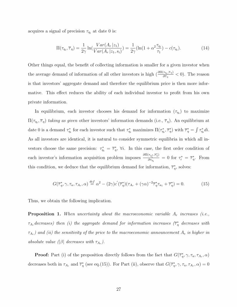
)− c(τηi). (14)
Other things equal, the benefit of collecting information is smaller for a given investor when
the average demand of information of all other investors is high (∂Π(τηi ,τη)
∂τη< 0). The reason
is that investors’ aggregate demand and therefore the equilibrium price is then more infor-
mative. This effect reduces the ability of each individual investor to profit from his own
private information.
In equilibrium, each investor chooses his demand for information (τηi) to maximize
Π(τηi , τ η) taking as given other investors’ information demands (i.e., τ η). An equilibrium at
date 0 is a demand τ ∗ηi for each investor such that τ ∗ηi maximizes Π(τ ∗ηi , τ∗η) with τ ∗η =
∫τ ∗ηidi.
As all investors are identical, it is natural to consider symmetric equilibria in which all in-
vestors choose the same precision: τ ∗ηi = τ ∗η, ∀i. In this case, the first order condition of
each investor’s information acquisition problem imposes∂Π(τη∗
i,τ∗η)
∂τηi= 0 for τ ∗i = τ ∗η. From
this condition, we deduce that the equilibrium demand for information, τ ∗η, solves:
G(τ ∗η, γ, τu, τAr , α)def= α2 − (2γ)c
′(τ ∗η)(τAr + (γα)−2τ ∗ητu1 + τ ∗η) = 0. (15)
Thus, we obtain the following implication.
Proposition 1. When uncertainty about the macroeconomic variable Ar increases (i.e.,
τArdecreases) then (i) the aggregate demand for information increases (τ ∗η decreases with
τAr) and (ii) the sensitivity of the price to the macroeconomic announcement Ae is higher in
absolute value (|β| decreases with τAr).
Proof: Part (i) of the proposition directly follows from the fact that G(τ ∗η, γ, τu, τAr , α)
decreases both in τAr and τ ∗η (see eq.(15)). For Part (ii), observe that G(τ ∗η, γ, τu, τAr , α) = 0
27

implies:
τ ∗1 = (τAr + (γα)−2τ ∗η(τAr)τu1) =α2
2γc′(τ ∗η(τAr))− α2τ ∗η(τAr). (16)
It follows from the second equality and the fact that τ ∗η(τAr) decreases with τAr that τ ∗1
increases with τAr . Thus, as |β| = |α|τετε+τ∗1
(see eq.(13)), we deduce that |β| decreases with τAr
as well.�
In sum, when market participants are more uncertain about the actual value of the
macroeconomic variable Ar, both the demand for information and the sensitivity of prices
to macroeconomic announcements about Ar increases. The true effect of the increase in
information demand is to dampen the effect of uncertainty on the sensitivity of the price
response to macroeconomic announcements. However, in equilibrium, this effect does not
fully offset the direct positive effect of an increase in uncertainty about Ar on |β|. As
a result, empirically, |β| and the aggregate demand for information before macroeconomic
announcements appear positively correlated, as we find in the data. This positive correlation
would disappear (and become negative) if one could control for investors’ prior uncertainty
about Ar. However, this is notoriously difficult. In fact, our results suggest that investors’
demand for information ahead of macroeconomic announcements, as proxied by clicks on
links to news referring to these announcements, can serve as a proxy for this uncertainty.
Kim and Verrecchia (1991a) develop a model of trading ahead of public news arrivals
in which investors’ information acquisition is endogenous. However, they do analyze the
effect of an increase in prior uncertainty about the asset payoff on the price reaction to
public news arrival. It can be checked that their model predicts no effect of such an increase
because of the particular specification of the cost of acquiring information in their model.
Our model is very similar to theirs but simpler and predicts that when uncertainty increases,
both information demand and the reaction of prices to public news arrival should increase.
28

5.2 Does demand for information increase with macroeconomic
uncertainty?
According to the model, the positive correlation between the strength of treasury price
reactions to surprises in nonfarm payroll announcements and information demand reflects
the fact that information demand is high when macroeconomic uncertainty is high. Thus, if
our interpretation is correct, we should observe a positive correlation between measures of
macroeconomic uncertainty and our proxy for information demand ahead of nonfarm payroll
announcements. To study this point, we estimate following equation:
AbnormalInformationDemandt = α + βXXt + εt, (17)
where the dependent variable, AbnormalInformationDemandt, is the ratio of the num-
ber of nonfarm payroll clicks on day t to the average of the variable in the last 40-business
days, so that the last nonfarm payroll announcement is included in the calculation. The
vector of explanatory variables, Xt, include all variables used as explanatory variables in our
price reaction regressions with three differences. First, we do not control for nonfarm payroll
surprises. Second, we include a dummy variable equal to 1 on nonfarm payroll announcement
days. last, we control for daily abnormal trading volume and realized volatility (defined as
the ratio of each variable on day t divided by their average value of the 40 last days).
[Insert Table 11 about Here]
Table 11 reports estimates of eq.(17). We find that information demand about nonfarm
payroll is significantly positively correlated with our market-based measure of macroeconomic
uncertainty. It is also positively correlated with the news-based measure but the correlation
is not significantly different from zero. Other variables are in general not significant, except
the supply of news related to nonfarm payroll. Not surprisingly, the supply and demand
of information about nonfarm payroll figures are positively related. Prior literature has
29

shown that investor attention is related to information supply, trading volume and asset
price volatility, but we are the first to show that it is also correlated with macroeconomic
uncertainty.
5.3 Investors’ sentiment or rational information demand?
Researchers have often used search data on the internet as a proxy for investors’ sentiment
rather than a proxy for information demand.27 In line with this interpretation, researchers
show that high search intensity for a given stock predict price reversals in this stock (see
Da, Engelberg, and Gao, 2011). In contrast to this literature, we use readership data,
not search data, and we argue that these data are associated with rational information
demand rather than investor sentiment. If our interpretation is correct, a high demand for
nonfarm payroll information on the day of nonfarm payroll announcements should not predict
subsequent price reversals (i.e., be positively associated with overreaction to macroeconomic
announcements).
[Insert Figure 5 about Here]
To give a first look at this issue, we plot in Figure 5, cumulative returns on nonfarm
payroll announcement days from two hours before the announcement up to 5 hours after the
announcement, separately for days with (i) positive or negative surprises) and (ii) a high
number of nonfarm payroll clicks (higher than the median) or a low number of nonfarm
payroll clicks. The figure shows three things. First, it confirms visually our main finding:
nonfarm payroll announcements have a much larger impact on treasury prices when the
number of nonfarm payroll clicks is high than on days in which this number is low. Second,
there is no sign of under or overreaction of treasury prices to nonfarm payroll announcements
after the announcement, whether the number of nonfarm payroll clicks is high or low. Last,
there is small price drift before the announcement, in the direction of the price jump at
27Investor sentiment, defined as in Baker and Wurgler (2007), is a belief about future cash flows andinvestment risks that is not justified by the facts at hand.
30

the announcement, especially for positive surprises when nonfarm payroll clicks is high.28
These two last observations are consistent with the view that these clicks proxy for rational
information demand rather than investors’ sentiment.
We now examine the preliminary evidence provided by Figure 5 more formally. First, to
estimate whether there is a post-announcement reversal we estimate the following equation:
DailyReturnt = α+30∑
i=−30
βSiSurpriset−i +30∑
i=−30
βBSiSurpriset−i×HighBitlyCountt−i + εt,
(18)
This specification is similar to that of Lucca and Moench (2015) except that we interact leads
and lags of the surprise variable by our proxy for information demand (HighBitlyCount).
results are reported in Table 12.
[Insert Table 12]
We find no evidence of post announcement drift for nonfarm payroll announcements: the
first lead coefficient on the surprise (βS−1) and the sum of the 30 lead coefficients are not
statistically significant. This conclusion is unchanged for the coefficients on the interaction
terms with the number of nonfarm payroll Bitly clicks. Similarly, we find no evidence of
pre announcement drift for nonfarm payroll announcements, at least at the daily frequency.
However, (Figure 5 suggests that one must zoom on minutes before the announcement to
detect the drift).
We next consider whether the response to the nonfarm payroll announcement persists
after one-week of the release and whether the persistence of the impact is related to high
Bitly counts. We estimate the equation:
WeeklyReturnt = α + βSSurpriset + βSBSurpriset ×HighBitlyCountt + εt, (19)
28This finding is consistent with Kurov, Sancetta, Strasser, and Wolfe (2016), who find evidence of preannouncement price drift ahead of various macroeconomic announcements. They argue that this drift reflectstrading on private information, which is consistent with our interpretation.
31

where WeeklyReturnt is estimated from the close of Thursday before the announcement
to the following Thursday. We drop 3 announcements out of the 66 because they were not
released on a Friday. The results are reported in Table 13. The coefficient on nonfarm
payroll surprises is statistically not significant for all maturities. Intuitively, over one week,
the flow of news affecting treasury prices is so intense that the effect of macroeconomic
announcements on price changes cannot be detected at this frequency. This highlights the
importance of estimating the effect of macro news on treasury prices using very narrow time
intervals around the arrival of news (see Andersen, Bollerslev, Diebold, and Vega (2003) and
Andersen, Bollerslev, Diebold, and Vega (2007)). However, the coefficient on the interaction
with Bitly is negative and statistically significant for all maturities. This finding shows, in
another way, that a high number of Bitly nonfarm payroll clicks has a strong effect on the
reaction of treasury prices to nonfarm payroll announcements, so large that the price reaction
to the announcement can still be statistically detected one week after the announcement.
Overall, the findings in Tables 12 and 13 do not suggest that there is systematic over
or under reaction of treasury prices to nonfarm payroll announcements or that overreaction
occurs when the number of Bitly nonfarm payroll clicks. Overall, this suggests that this
number is not a proxy for investors’ sentiment.
Next, we investigate more formally our conjecture that the number of Bitly nonfarm
payroll clicks is a proxy for the acquisition of private information about the effect of nonfarm
payroll figures on treasury prices. If this is the case then the model implies that the price
impact of trades before nonfarm payroll announcements should be higher on days in which
the number of Bitly nonfarm payroll clicks is high. Indeed, in the model, this impact is
measured by αλ. From the expression for lambda, we deduce that the price impact of
the order flow at date 1 (i.e., D(p1∗)) increases with (i) macroeconomic uncertainty (τ−1Ar
)
and (ii) information demand (τη), other things equal. As an increase in macro-uncertainty
itself foster information demand, the combination of these two effects implies that the price
32

impact of trades before nonfarm payroll announcements should be higher on days in which
the number of Bitly nonfarm payroll clicks is high.
To study whether this is the case, we define OrderF lowτt as the order flow imbalance
(the difference between buy and sell market orders, signed using the Lee and Ready (1991)
algorithm) over interval [τ, τ+1] on day t, where each interval has a one minute duration and
τ = 0 is the time at which the announcement takes place. We then estimate the following
equation:
OneMinuteReturnτt = α+βSSurpriset+IB(λBOrderF lowτt+κBHighBitlyCountt×OrderF lowt)+
IA(λAOrderF lowτt + κAHighBitlyCountt ×OrderF lowt) + εt, (20)
where IB is a dummy variable equal to one if τ < 0 (before the announcement) and IA is a
dummy variable equal to one if τ ≥ 0 (after the announcement). Thus, λB and λA measure,
respectively, the price impact of trades before and after nonfarm payroll releases while κB
and κA measures the effect of the number of Bitly clicks on the price impact of trades before
and after nonfarm payroll releases, respectively. Our specification for measuring the price
impact of trades around nonfarm payroll announcements is similar to that used in Brandt
and Kavajecz (2004) and Pasquariello and Vega (2007). We report estimates of eq.(20) in
Table 14.
[Insert Table 14]
We find that the impact of trades is significant both before and after nonfarm payroll re-
leases for all maturities, suggesting that trades contain information both before and after
these releases. However, trades are more informative after nonfarm payroll announcements
than before. Overall these findings are consistent with Brandt and Kavajecz (2004) and
Pasquariello and Vega (2007), who find evidence of informed trading in treasury markets
on macroeconomic announcement days. More importantly for our purpose, we find that the
33

impact of order flow is significantly stronger when the number of Bitly clicks is high. This ef-
fect is always statistically significant after nonfarm payroll announcements. It is statistically
significant before nonfarm payroll announcements only for two year and ten year treasuries.
Overall these findings are consistent with the view that (i) there is informed trading around
macroeconomic announcements in treasury markets and (ii) the number of Bitly clicks is a
proxy for private information acquisition by investors.
6 Conclusion
We measure demand for information prior to nonfarm payroll announcements using a novel
dataset consisting of clicks on news articles. We find that when information demand is high
shortly before the release of nonfarm payroll announcements, the price response of U.S. Trea-
sury note futures to nonfarm payroll news surprises doubles. We show that this relationship
is consistent with Bayesian learning models of information acquisition. Namely, market par-
ticipants collect more information about macroeconomic variables affecting treasury prices
when uncertainty about these variables is higher. As treasury prices respond more strongly
to news when macroeconomic uncertainty is high, this behavior leads to a positive corre-
lation between measures of information demand and treasuries price responses to nonfarm
payroll announcements.
Overall, this finding suggest that greater investor attention (demand for information) can
affect not only price discovery after news arrival (as found in the literature) but also before
news arrival. Moreover, shifts in this attention prior to macroeconomic news release might
be used to measure shifts in market participants perception of economic uncertainty. One
possible venue for future research is to check the external validity of our findings (i.e., that
they are valid for other types of scheduled news).
34

References
Andersen, T., and T. Bollerslev (1998): “Deutsche mark-dollar volatility: intra-dayactivity patterns, macroeconomic announcements, and longer run dependencies,” Journalof Finance, 53, 219–265.
Andersen, T. G., T. Bollerslev, F. X. Diebold, and C. Vega (2003): “Microeffects of macro announcements: Real-time price discovery in foreign exchange,” AmericanEconomic Review, 93(1), 38–62.
(2007): “Real-Time Price Discovery in Global Stock, Bond and Foreign ExchangeMarkets,” Journal of International Economics, 73, 251–277.
Baker, M., and J. Wurgler (2007): “Investor Sentiment in the Stock Market,” Journalof Economic Perspectives, 21, 129–157.
Baker, S., N. Bloom, and S. J. Davis (2016): “Measuring Economic Policy Uncer-tainty,” Quaterly Journal of Economics, 131, 1593–1636.
Balduzzi, P., E. J. Elton, and T. C. Green (2001): “Economic News and BondPrices: Evidence From the U.S. Treasury Market,” Journal of Financial and QuantitativeAnalysis, 36(4), 523–543.
Beechey, M. J., and J. H. Wright (2009): “The High-Frequency Impact of News onLong-Term Yields and Forward Rates: Is It Real?,” Journal of Monetary Economics,56(4), 535–544.
Ben-Rephael, A., Z. Da, and R. D. Israelsen (2017): “It Depends on Where YouSearch: Institutional Investor Attention and Underreaction to News,” Review of FinancialStudies, 30(9), 3009–3047.
Bernile, G., J. Hu, and Y. Tang (2016): “Can information be locked up? Informedtrading ahead of macro-news announcements,” Journal of Financial Economics.
Brandt, M., and K. Kavajecz (2004): “Price Discovery in the U.S. Treasury Market:The Impact of Orderflow and Liquidity on the Yield Curve,” Journal of Finance, 59,2623–2654.
Carlston, B., and M. Ochoa (2017): “Macroeconomic Announcements and InvestorBeliefs at the Zero Lower Bound,” Discussion paper, Working Paper.
Chan, W. S. (2003): “Stock price reaction to news and no-news: drit and reversal afterheadlines,” Journal of Financial Economics, 70, 223–260.
Da, Z., J. Engelberg, and P. Gao (2011): “In search of attention,” Journal of Finance,66(5), 1461–1499.
Dellavigna, S., and J. M. Pollet (2009): “Investor Inattention and Friday EarningsAnnouncements,” Journal of Finance, 64, 709–749.
35

Engelberg, J. E., and C. A. Parsons (2011): “The Causal Impact of Media in FinancialMarkets,” Journal of Finance, 66, 67–97.
Eugene A. Imhoff, J., and G. J. Lobo (1992): “The effect of ex ante earnings uncer-tainty on earnings response coefficients,” The Accounting Review, 67, 427–439.
Femia, K., S. Friedman, and B. Sack (2013): “The Effects of Policy Guidance onPerceptions of the Fed’s Reaction Function,” Discussion paper, Federal Reserve Bank ofNew York, Staff Report No. 652.
Fleming, M. J., and E. M. Remolona (1997): “What Moves the Bond Market?,”Economic Policy Review, 3(4), 31–50.
(1999): “Price Formation and Liquidity in the U.S. Treasury Market: The Responseto Public Information,” Journal of Finance, 54(5), 1901–1915.
Gilbert, T. (2011): “Information aggregation around macroeconomic announcements: Re-visions matter,” Journal of Financial Economics, 101, 114–131.
Gilbert, T., C. Scotti, G. Strasser, and C. Vega (2017): “Is the Intrinsic Value ofa Macroeconomic News Announcement Related to Its Price Impact,” Journal of MonetaryEconomics.
Goldberg, L., and D. Leonard (2003): “What Moves Sovereign Bond Markets? TheEffects of Economic News on U.S. and German Yields,” Current Issues in Economics andFinance, 9(9).
Goldberg, L. S., and C. Grisse (2013): “Time variation in asset price responses tomacro announcements,” Discussion paper, National Bureau of Economic Research.
Grossman, S., and J. Stiglitz (1980): “On the Impossibility of Informationally EfficientMarkets,” American Economic Review, 70, 393–408.
Gurkaynak, R. S., B. P. Sack, and E. T. Swanson (2005): “The Excess Sensitivityof Long-Term Interest Rates to Economic News: Evidence and Implications for Macroe-conomic Models,” American Economic Review, 95(1), 425–436.
Hautsch, N., and D. Hess (2007): “Bayesian learning in financial markets: testing forthe relevance of information precision in price discovery,” Journal of Financial and Quan-titative Analysis, 42, 189–208.
Hirshleifer, D., S. S. Lim, and S. H. Teoh (2008): “Driven to distraction: Extranousevents and underreaction to earnings news,” Journal of Finance, 64(5), 2289–2325.
Husted, L., J. Rogers, and B. Sun (2017): “Monetary Policy Uncertainty,” Discussionpaper, International Finance Discussion Papers No. 1215.
Kearney, M. S., and P. B. Levine (2015): “Media Influences on Social Outcomes: TheImpact of MTV’s 16 and Pregnant on Teen Childbearing,” American Economic Review,105, 3597–3632.
36

Kim, O., and R. E. Verrecchia (1991a): “Market reaction to anticipated announce-ments,” Journal of Financial Economics, 30, 273–309.
(1991b): “Trading Volume and Price Reactions to Public Announcements,” Journalof Accounting Research, 29, 302–321.
Kurov, A., A. Sancetta, G. Strasser, and M. H. Wolfe (2016): “Price drift beforeU.S. macroeconomic news: private information about public announcements?,” Discussionpaper, European Central Bank Working Paper Series No. 1901.
Lee, C. M. C., and M. J. Ready (1991): “Inferring Trade Direction from Intraday Data,”Journal of Finance, 46, 733–746.
Lucca, D. O., and E. Moench (2015): “The Pre-FOMC Announcement Drift,” Journalof Finance, 70, 329–371.
Pasquariello, P., and C. Vega (2007): “Informed and Strategic Order Flow in theBond Markets,” Review of Financial Studies, 20, 1975–2019.
Peress, J. (2014): “The media and the diffusion of information in financial markets: Evi-dence from newspaper strikes,” The Journal of Finance, 69(5), 2007–2043.
Peress, J., and D. Schmidt (2018): “Glued to the TV: Distracted Noise Traders andStock Market Liquidity,” Discussion paper, INSEAD.
Scotti, C. (2016): “Surprise and uncertainty indexes: Real-time aggregation of real-activity macro-surprises,” Journal of Monetary Economics, 82, 1–19.
Stephens-Davidowitz, S. (2013): “The Cost of Racial Animus on a Black PresidentialCandidate: Using Google Search Data to Find What Surveys Miss,” Discussion paper,Harvard University.
Swanson, E. T., and J. C. Williams (2014): “Measuring the Effect of the ZeroLower Bound on Medium-and Longer-Term Interest Rates,” American Economic Review,104(10), 3154–3185.
Tetlock, P. C. (2014): “Information Transmission in Finance,” Annual Review of Finan-cial Economics, 6, 365–348.
Veldkamp, L. L. (2006): “Media Frenzies in Markets for Financial Information,” AmericanEconomic Review, 96, 577–601.
Vives, X. (1995): “The Speed of Information Revelation in a Financial Maket Mechanism,”Journal of Economic Theory, 67, 178–204.
Vlastakis, N., and R. N. Markellos (2012): “Information Demand and Stock MarketVolatility,” Journal of Banking and Finance, 36(6), 1808–1821.
37

7 Appendix
Appendix A
In this appendix, we complete the derivations of the results obtained in Section 5.
Derivation of informed investors’ demand
Using the fact that investors have a CARA utility function, we deduce that the demand
of investor i is:
di(si, p1) =E(F |si, p1)− p1
γVar(F |si, p1)=
(E(Ar |si, z1)− E(Ar |z1))
γαVar(Ar |si, p1), (21)
where the second equality follows from the fact that (i) p1 = µ+ αE(Ar |si, z1) and (ii) z1 is
a sufficient statistics for p1. Moreover:
E(Ar |si, z1) = E(Ar |z1) +τηi
τηi + τ1
(si − E(Ar |z1)), (22)
and
Var(Ar |si, z1) =1
τηi + τ1
, (23)
where τ1 is defined in eq.( 11). Substituting eq.(22) and eq.(23) in eq.(21) and using the fact
that E(Ar |si, z1) = α−1(p1 − µ), we deduce that:
di(si, p1) = ai(αsi + µ− p1),
where ai is defined as in the text.
Derivation of the certainty equivalent of investor i’s expected utility at date 0.
Investors’ final wealth at date 3 is:
Wi3 = (F − p1)di(si, p1)− c(τηi). (24)
38

Conditional on p1 and si, Wi3 has anormal distribution. Thus:
E(− exp(−γWi3) |si, p1) = − exp(−γ(E(Wi3 |si, p1)− γ
2Var(Wi3 |si, p1))).
Using eq.(24), we obtain:
E(− exp(−γWi3) |si, p1) = − exp(−0.5γ2d2iVar(F |si, p1)− c(τηi).
Using the expression for di(si, p1) in eq.(21), we deduce that:
E(− exp(−γWi3)) = E(E(− exp(−γWi3) |si, p1))
= − exp(γc(τηi)
(1 + γ2Var(F |si, p1) Var(di))12
,
= − exp(γci(ηi))
(1 + Var(E(F |si,p1)−p1)Var(F |si,p1)
)12
.
Thus, the certainty equivalent of investor i’s expected utility is:
Πi(τηi , τ η) =1
2γln(1 +
Var(E(F |si, p1)− p1)
Var(F |si, p1))− c(τηi).
Now,
Var(E(F |si, p1)− p1)
Var(F |si, p1)=
α2τ 2ηi
(τηi + τ1)2
Var(si − E(Ar |p1) )
(τηi + τ1)−1
=α2τ 2
ηi
(τηi + τ1)Var(Ar − E(Ar |p1) + ηi)
=α2τ 2
ηi
(τηi + τ1)(τ−1ηi
+ τ−11 )
=α2τηiτ1
.
where the penultimate equality folllows from the fact that (i) Var(Ar−E(Ar |p1)) =Var(Ar |p1) =
τ−11 and (ii) Ar−E(Ar |p1) is independent from ηi.
39

Appendix B: Figures and Tables
Figure 1: Intra Day Bitly Counts on Nonfarm Payroll Announcement Days
04:00
05:00
06:00
07:00
08:00
09:00
10:00
11:00
12:00
13:00
14:00
15:00
16:00
17:00
time
0
200
400
600
800
1000
Bitly
cou
nts
Notes: The figure shows the per minute number of nonfarm payroll Bitly clicks from 4:00 am ET to 5:00 pm
ET, across all nonfarm payroll announcement days from January 2011 to June 2016 (66 days). The vertical
red line identifies the release time of nonfarm payroll, 8:30 am ET.
40

Figure 2: Bitly Daily Counts
2011 2012 2013 2014 2015 2016time
0
500
1000
1500
2000
2500
Bitly
cou
nts
Notes: The figure shows the number of daily clicks in the Bitly dataset on headlines containing the word
payroll for all days in our sample. The vertical black lines identify nonfarm payroll event days. the vertical
red line identifies September 8, 2011, when President Obama announced a $447 billion jobs plan.

Figure 3: Comparing Different Measures of Information Demand: Bitly Counts and GoogleTrend Index
(a) Weekly Frequency
2011-01 2012-01 2013-01 2014-01 2015-01 2016-01time
0
20
40
60
80
100
Goog
le in
dex
correlation = 0.68
0
500
1000
1500
2000
2500
3000
Bitly
cou
nts
Google indexBitly counts
(b) Weeks with a Nonfarm Payroll Announcement Release
2011-01 2012-01 2013-01 2014-01 2015-01 2016-01time
30
40
50
60
70
80
90
100
Goog
le in
dex
correlation = 0.38
0
500
1000
1500
2000
2500
3000
Bitly
cou
nts
Google indexBitly counts
Notes: Panel a shows weekly Bitly counts and Google Trend Index for all the weeks in our sample from
January 2011 to June 2016. Panel b shows weekly Bitly counts and Google Trend index for weeks when
there was a nonfarm payroll release (a total of 66 weeks). The Bitly counts are based on headlines containing
the word payroll, and the Google Trend Index is for the topic nonfarm payroll.
42

Figure 4: Information Demand and Supply: Bitly Counts and Ravenpack News Counts
(a) Daily Frequency
2011-01 2012-01 2013-01 2014-01 2015-01 2016-01time
0
10
20
30
40
50
60
70
80
Rave
npac
k co
unts
correlation = 0.67
0
500
1000
1500
2000
2500
Bitly
cou
nts
Ravenpack countsBitly counts
(b) Days with a Nonfarm Payroll Announcement Release
2011-01 2012-01 2013-01 2014-01 2015-01 2016-01time
0
10
20
30
40
50
60
70
80
Rave
npac
k co
unts
correlation = 0.13
0
500
1000
1500
2000
2500
Bitly
cou
nts
Ravenpack countsBitly counts
Notes: Panel a shows daily Bitly counts and Ravenpack news counts for all the days in our sample from
January 2011 to June 2016. Panel b shows daily Bitly counts and Ravenpack news counts on days with
a nonfarm payroll release (66 days). The Bitly counts and Ravenpack news counts are based on headlines
containing the word payroll.

Figure 5: Intra Day Treasury Price Reaction and Bitly Nonfarm Payroll Clicks
−8
−6
−4
−2
0
2
4
6
8
−120 −100 −80 −60 −40 −20 0 20 40 60 80 100 120 140 160 180 200 220 240 260 280 300 320 340 360event time (minutes)
cum
ulat
ive
retu
rn (
bps)
CategoryNeg Surprise−Low Bitly Neg Surprise−High BitlyPos Surprise−Low Bitly Pos Surprise−High Bitly
Notes: The figure shows the intraday reaction of the two-year U.S. Treasury futures prices to nonfarm payroll
surprises from January 2011 to June 2016 (a total of 66 days). We perform a dependent sort on surprise and
Bitly counts. Time 0 on the x-axis indicates the release time of nonfarm payroll, at 8:30 am ET.
44

Tab
le1:
Pop
ula
rN
ews
Sou
rces
ofA
rtic
les
Shar
edusi
ng
Bit
ly
New
sSou
rce
UR
LN
um
ber
ofC
lick
sP
erce
nt
ofT
otal
Num
ber
ofC
lick
sC
um
ula
tive
Per
cent
Pan
elA
:P
rior
tonon
farm
pay
roll
rele
ase,
from
6:25
amto
8:25
amB
loom
ber
gw
ww
.blo
omb
erg.
com
3,43
873
73M
arke
twat
chw
ww
.mar
ketw
atch
.com
340
780
Wal
lStr
eet
Jou
rnal
ww
w.w
sj.c
om27
76
86F
inan
cial
Tim
esw
ww
.ft.
com
221
591
USA
Today
ww
w.u
sato
day
.com
173
495
CN
BC
ww
w.c
nb
c.co
m15
33
98
Pan
elB
:D
uri
ng
and
afte
rnon
farm
pay
roll
rele
ase,
from
8:26
amto
10:2
6am
Blo
omb
erg
ww
w.b
loom
ber
g.co
m26
,235
6767
CN
BC
ww
w.c
nb
c.co
m5,
769
1582
Reu
ters
ww
w.r
eute
rs.c
om1,
860
587
Mar
ketw
atch
ww
w.m
arke
twat
ch.c
om1,
265
390
Wal
lStr
eet
Jou
rnal
ww
w.w
sj.c
om1,
173
393
USA
Today
ww
w.u
sato
day
.com
772
295
Not
es:
Ou
rsa
mp
lep
erio
dis
from
Jan
uar
y20
11to
Ju
ne
2016,
wh
ich
incl
ud
esa
tota
lof
66
non
farm
pay
roll
an
nou
nce
men
ts.
InP
an
elA
,w
eco
nsi
der
clic
ks
two
hou
rsp
rior
toth
ere
leas
eof
the
non
farm
pay
roll
an
nou
nce
men
t,fr
om
6:2
5am
to8:2
5am
ET
.T
her
eare
ato
tal
of
4,6
85
clic
ks
du
rin
g
this
per
iod
acro
ssth
e66
ann
oun
cem
ents
.In
Pan
elB
,w
eco
nsi
der
clic
ks
du
rin
gan
daft
erth
ean
nou
nce
men
t,fr
om
8:2
6am
to10:2
6am
ET
.T
her
e
are
ato
tal
of38
,963
clic
ks
du
rin
gth
isp
erio
dac
ross
the
66
an
nou
nce
men
ts.
Th
en
on
farm
pay
roll
an
nou
nce
men
tis
rele
ase
dby
the
Bu
reau
of
Lab
or
Sta
tist
ics
at8:
30am
ET
onth
efi
rst
Fri
day
ofth
em
onth
.
45

Tab
le2:
Who
Shar
esB
itly
Lin
ks
Bit
lyU
ser
Typ
eN
um
ber
ofC
lick
sP
erce
nt
ofT
otal
Num
ber
ofC
lick
sC
um
mula
tive
Per
cent
Pan
elA
:P
rior
tonon
farm
pay
roll
rele
ase,
from
6:25
amto
8:25
amO
ffici
alB
loom
ber
gU
sers
2,50
854
54Sev
enIn
div
idual
Use
rs1,
349
2983
Offi
cial
WSJ
Use
rs20
14
87O
ffici
alU
SA
Today
Use
rs17
34
91O
ffici
alM
arke
twat
chU
sers
148
394
Offi
cial
CN
BC
Use
rs74
296
Offi
cial
FT
Use
rs57
197
Offi
cial
Reu
ters
Use
rs8
0.2
96.2
Pan
elB
:D
uri
ng
and
afte
rnon
farm
pay
roll
rele
ase,
from
8:26
amto
10:2
6am
Offi
cial
Blo
omb
erg
Use
rs18
,228
4747
Sev
enIn
div
idual
Use
rs10
,485
2774
Offi
cial
CN
BC
Use
rs3,
914
1084
Offi
cial
Reu
ters
Use
rs1,
528
488
Offi
cial
WSJ
Use
rs1,
031
394
Offi
cial
USA
Today
Use
rs66
92
96O
ffici
alN
PR
Use
rs63
52
97O
ffici
alM
arke
twat
chU
sers
257
198
Not
es:
Ou
rsa
mp
lep
erio
dis
from
Jan
uar
y20
11to
Ju
ne
2016,
wh
ich
incl
ud
esa
tota
lof
66
non
farm
pay
roll
an
nou
nce
men
ts.
InP
an
elA
,w
eco
nsi
der
clic
ks
two
hou
rsp
rior
toth
ere
leas
eof
the
non
farm
pay
roll
an
nou
nce
men
t,fr
om
6:2
5am
to8:2
5am
ET
.T
her
eare
ato
tal
of
4,6
85
clic
ks
du
rin
g
this
per
iod
acro
ssth
e66
ann
oun
cem
ents
.In
Pan
elB
,w
eco
nsi
der
clic
ks
du
rin
gan
daft
erth
ean
nou
nce
men
t,fr
om
8:2
6am
to10:2
6am
ET
.T
her
e
are
ato
tal
of38
,963
clic
ks
du
rin
gth
isp
erio
dac
ross
the
66
an
nou
nce
men
ts.
Th
en
on
farm
pay
roll
an
nou
nce
men
tis
rele
ase
dby
the
Bu
reau
of
Lab
or
Sta
tist
ics
at8:
30am
ET
onth
efi
rst
Fri
day
ofth
em
onth
.W
eaggre
gate
clic
ks
on
lin
ks
share
dby
seve
ndiff
eren
tin
div
idu
al
use
rs.
New
sse
rvic
esoft
en
hav
em
ore
than
one
Bit
lyu
ser
acco
unt.
Inge
ner
al,
on
eB
itly
use
racc
ou
nts
for
the
majo
rity
of
the
clic
ks,
bu
tw
eaggre
gate
acr
oss
offi
cial
use
rsw
ith
in
an
ews
serv
ices
.T
he
list
ofoffi
cial
use
rnam
esp
ern
ews
serv
ice
was
pro
vid
edto
us
by
Bit
ly.
46

Tab
le3:
Cou
ntr
yof
IPA
ddre
ssof
the
Rea
der
ofB
itly
Lin
ks
Cou
ntr
yof
IPA
ddre
ssN
um
ber
ofC
lick
sP
erce
nt
ofT
otal
Num
ber
ofC
lick
sC
um
mula
tive
Per
cent
Pan
elA
:P
rior
tonon
farm
pay
roll
rele
ase,
from
6:25
amto
8:25
amU
nit
edSta
tes
2,25
148
48U
nknow
n53
211
59G
reat
Bri
tain
271
665
Can
ada
155
368
Jap
an13
13
71G
erm
any
912
73In
dia
882
75Spai
n81
277
Pan
elB
:D
uri
ng
and
afte
rnon
farm
pay
roll
rele
ase,
from
8:26
amto
10:2
6am
Unit
edSta
tes
20,7
2953
53U
nknow
n2,
676
760
Jap
an2,
668
773
Gre
atB
rita
in1,
190
363
Can
ada
1,03
33
66Sin
gap
ore
829
22
India
730
276
Ger
man
y67
42
74
Not
es:
Ou
rsa
mp
lep
erio
dis
from
Jan
uar
y20
11to
Ju
ne
2016,
wh
ich
incl
ud
esa
tota
lof
66
non
farm
pay
roll
an
nou
nce
men
ts.
InP
an
elA
,w
eco
nsi
der
clic
ks
two
hou
rsp
rior
toth
ere
leas
eof
the
non
farm
pay
roll
an
nou
nce
men
t,fr
om
6:2
5am
to8:2
5am
ET
.T
her
eare
ato
tal
of
4,6
85
clic
ks
du
rin
g
this
per
iod
acro
ssth
e66
ann
oun
cem
ents
.In
Pan
elB
,w
eco
nsi
der
clic
ks
du
rin
gan
daft
erth
ean
nou
nce
men
t,fr
om
8:2
6am
to10:2
6am
ET
.T
her
e
are
ato
tal
of38
,963
clic
ks
du
rin
gth
isp
erio
dac
ross
the
66
an
nou
nce
men
ts.
Th
en
on
farm
pay
roll
an
nou
nce
men
tis
rele
ase
dby
the
Bu
reau
of
Lab
or
Sta
tist
ics
at8:
30am
ET
onth
efi
rst
Fri
day
ofth
em
onth
.T
he
acc
ura
cyof
the
geo
loca
tion
of
IPad
dre
sses
isfa
irly
acc
ura
te,
bu
tn
ot
per
fect
.
47

Tab
le4:
How
are
Bit
lyL
inks
Acc
esse
d
How
are
links
acce
ssed
Num
ber
ofC
lick
sP
erce
nt
ofT
otal
Num
ber
ofC
lick
sC
um
mula
tive
Per
cent
Pan
elA
:P
rior
tonon
farm
pay
roll
rele
ase,
from
6:25
amto
8:25
amT
wit
ter
2,33
850
50D
irec
tly
1,92
841
91F
aceb
ook
261
697
Goog
le29
198
Fin
anci
alT
imes
160.
398
.3Sto
ckT
wit
s16
0.3
98.6
Mar
ket
Ear
lyB
ird
110.
298
.8
Pan
elB
:D
uri
ng
and
afte
rnon
farm
pay
roll
rele
ase,
from
8:26
amto
10:2
6am
Tw
itte
r17
,690
4545
Dir
ectl
y16
,046
4186
Fac
ebook
3,81
910
96G
oog
le50
81
97D
aily
FX
880.
297
.2H
oot
Suit
e56
0.1
97.3
Mar
ket
Ear
lyB
ird
420.
197
.4
Not
es:
Ou
rsa
mp
lep
erio
dis
from
Jan
uar
y20
11to
Ju
ne
2016,
wh
ich
incl
ud
esa
tota
lof
66
non
farm
pay
roll
an
nou
nce
men
ts.
InP
an
elA
,w
eco
nsi
der
clic
ks
two
hou
rsp
rior
toth
ere
leas
eof
the
non
farm
pay
roll
an
nou
nce
men
t,fr
om
6:2
5am
to8:2
5am
ET
.T
her
eare
ato
tal
of
4,6
85
clic
ks
du
rin
g
this
per
iod
acro
ssth
e66
ann
oun
cem
ents
.In
Pan
elB
,w
eco
nsi
der
clic
ks
du
rin
gan
daft
erth
ean
nou
nce
men
t,fr
om
8:2
6am
to10:2
6am
ET
.T
her
e
are
ato
tal
of38
,963
clic
ks
du
rin
gth
isp
erio
dac
ross
the
66
an
nou
nce
men
ts.
Th
en
on
farm
pay
roll
an
nou
nce
men
tis
rele
ase
dby
the
Bu
reau
of
Lab
or
Sta
tist
ics
at8:
30am
ET
onth
efi
rst
Fri
day
ofth
em
onth
.L
inks
that
are
acc
esse
dd
irec
tly
are
lin
ks
that
are
cop
ied
an
dp
ast
edby
the
ind
ivid
ual
into
the
bro
wse
r.T
hey
cou
ldh
ave
rece
ived
the
lin
kvia
SM
Ste
xt,
e-m
ail
or
saw
the
lin
kon
Tw
itte
r,b
ut
rath
erth
an
clic
kon
itu
sin
gT
wit
ter,
cop
ied
an
d
pas
ted
the
lin
kin
toa
bro
wse
r.
48

Table 5: Summary Statistics
Obs. Mean Std. Deviation Min. Max.
Panel A: January 2004 to June 2016
Monetary Policy Variables
Federal Funds Rate 150 1.49 1.81 0.25 5.25
Swanso-Williams ZLB 150 0.11 0.32 0 1
Market-based Policy Uncertainty 150 85.67 30.53 32.05 158.97
News-based Policy Uncertainty 150 139.73 71.02 30.8 377.41
Risk
VIX Index 150 19.08 8.91 10.08 59.93
Information Environment
Nonfarm Payroll Surprise 150 -10.22 69.71 -208 188
Revision Noise 150 27.61 22.68 0 125
Forecast Error 150 55.10 43.68 1 208
Analyst Forecast Dispersion 150 0.26 0.49 0.07 5.33
Trading Volume and VolatilityTwo-Year US Treasury Trading Volume 150 0.21 0.12 0.01 0.50
Two-Year US Treasury Realized Volatility 150 2.39 1.53 0.39 10.02
Panel B: January 2011 to June 2016
Monetary Policy Variables
Federal Funds Rate 66 0.27 0.07 0.25 0.5
Swanso-Williams ZLB 66 0.26 0.44 0 1
Market-based Policy Uncertainty 66 60.85 16.70 32.05 105.74
News-based Policy Uncertainty 66 169.31 74.58 57.45 377.41
Risk
VIX Index 66 17.04 5.59 10.32 36.2
Information Environment
Nonfarm Payroll Surprise 66 -3.48 58.65 -123 103
Revision Noise 66 24.35 16.27 1 77
Forecast Error 66 46.91 34.90 1 123
Analyst Forecast Dispersion 66 0.16 0.08 0.09 0.51
Trading Volume and Volatility
Two-Year US Treasury Trading Volume 66 0.25 0.10 0.08 0.50
Two-Year US Treasury Realized Volatility 66 1.50 0.78 0.39 3.82
Information Demand and Supply
Intraday Bitly Counts (Before Announcement) 66 52 85 0 413
Intraday Bitly Counts (During Announcement) 66 398 311 1 1385
Weekly Google Trend Index 66 57 13 31 100
Ravenpack News Count 66 22 11 3 79
Notes: In Panel A our sample period is from January 2004 to June 2016 during non-farm payroll announce-
ment days. In Panel A our sample period is from January 2011 to June 2016 during nonfarm payroll
announcement days. The units of trading volume are million of contracts.
49

Tab
le6:
U.S
.T
reas
ury
Futu
res
Res
pon
seto
Non
farm
Pay
roll
Surp
rise
s
(1)
(2)
(3)
Jan
.20
04-
Jun.
2016
Jan
.20
11-
Jun.
2016
Jan
.20
11-
Jun.
2016
(excl
ud.
SW
ZL
Bp
erio
d)
Res
pon
seof
the
Tw
o-Y
ear
U.S
.T
reas
ury
Not
eF
utu
res
Non
farm
Pay
roll
Surp
rise
-11.
00**
*-6
.613
***
-8.0
20**
*(0
.904
)(0
.964
)(1
.183
)C
onst
ant
-0.7
860.
255
0.07
05(0
.745
)(0
.660
)(0
.833
)N
um
ber
ofO
bse
rvat
ions
150
6649
Adju
sted
R-s
quar
ed0.
500
0.42
40.
494
Res
pon
seof
the
Fiv
e-Y
ear
U.S
.T
reas
ury
Not
eF
utu
res
Non
farm
Pay
roll
Surp
rise
-29.
81**
*-2
8.17
***
-30.
92**
*(2
.135
)(3
.220
)(4
.013
)C
onst
ant
-1.6
510.
759
0.21
6(1
.759
)(2
.203
)(2
.826
)N
um
ber
ofO
bse
rvat
ions
150
6649
Adju
sted
R-s
quar
ed0.
568
0.54
50.
558
Res
pon
seof
the
Ten
-Yea
rU
.S.
Tre
asury
Not
eF
utu
res
Non
farm
Pay
roll
Surp
rise
-41.
58**
*-4
3.93
***
-44.
93**
*(2
.938
)(4
.728
)(5
.854
)C
onst
ant
-3.6
29-0
.449
-0.9
90(2
.421
)(3
.234
)(4
.123
)N
um
ber
ofO
bse
rvat
ions
150
6649
Adju
sted
R-s
quar
ed0.
575
0.57
40.
556
Not
es:
We
show
esti
mat
esof
equ
atio
n1
usi
ng
thre
ed
iffer
ent
sam
ple
s.In
colu
mn
1,
the
sam
ple
isfr
om
Janu
ary
2004
toJu
ne
2016.
Inco
lum
n2,
the
sam
ple
isfr
omJan
uar
y20
11to
Ju
ne
2016
,th
esa
mp
lefo
rw
hic
hw
eh
ave
Bit
lyd
ata
.In
colu
mn
3,
we
use
the
short
ersa
mp
le,
from
Janu
ary
2011
to
Ju
ne
2016
,an
dex
clu
de
the
Sw
anso
n-W
illi
ams
per
iod
wh
entw
o-y
ear
U.S
.T
reasu
ryn
ote
yie
lds
resp
ond
edle
ssto
macr
oec
on
om
icn
ews
an
nou
nce
men
ts
bec
ause
ofth
eZ
ero
Low
erB
oun
d.
50

Table 7: Response of the Two-Year US Treasury Futures to Nonfarm Payroll Surprises: LongSample Period
(1) (2) (3) (4) (5) (6)
NFP Surprise -10.73*** -1.646 -16.03*** -7.711*** -14.34*** -1.345
(1.230) (4.293) (1.760) (1.907) (2.926) (4.607)
Monetary Policy Variables
NFP Surprise x FFR Level -0.798 -0.0496
(0.631) (0.631)
NFP Surprise x Swanson-Williams Period 9.419** 0.624
(3.621) (3.752)
NFP Surprise x Market-implied Uncertainty -0.112*** -0.179***
(0.0302) (0.0477)
NFP Surprise x News-based Uncertainty 0.0129 -0.0116
(0.0161) (0.0172)
Risk
NFP Surprise x VIX Index 0.241*** 0.403***
(0.0730) (0.139)
Information Environment
NFP Surprise x Past Revision Noise 0.0432 -0.0330
(0.0306) (0.0411)
NFP Surprise x Past Forecast Errors -6.695*** -1.357
(1.618) (1.928)
NFP Surprise x Past Forecast Dispersion -0.679 -1.891
(3.035) (3.047)
Trading Volume and Volatility
NFP Surprise x Past Trading Volume 32.36*** 5.006
(10.18) (13.71)
NFP Surprise x Past Realized Volatility -0.614 1.273
(1.692) (2.714)
Constant -0.217 -0.803 -0.658 0.835 -1.375 -1.412
(1.029) (2.957) (0.722) (1.518) (2.521) (3.352)
Number of observations 150 150 150 150 150 150
R-squared 0.537 0.568 0.534 0.583 0.546 0.676
Notes: We estimate the response of U.S. Treasury futures on two-year notes to nonfarm payroll surprises
using data from January 2004 to June 2016. The dependent variable is a 10-minute U.S. Treasury futures
return using the prevailing futures price as of five minutes before the announcement to five minutes after the
announcement. The estimation also includes main effects, but we do not report these coefficients. Standard
errors are in parentheses. ***, **, * denote statistical significance at the 1%, 5%, and 10% level, respectively.
51

Table 8: Response of the Two-Year US Treasury Futures to Nonfarm Payroll Surprises
(1) (2) (3) (4) (5) (6)
NFP Surprise -3.401 -8.281** -9.970*** -9.985 -0.956 -2.817
(6.328) (3.814) (2.763) (9.312) (1.955) (13.40)
Monetary Policy Variables
NFP Surprise x FFR Level -0.362 -9.528
(15.61) (20.49)
NFP Surprise x Swanson-Williams Period 5.727* 4.052
(2.941) (4.822)
NFP Surprise x Market-implied Uncertainty -0.0387 -0.0812
(0.0694) (0.114)
NFP Surprise x News-based Uncertainty -0.0115 -0.000145
(0.0177) (0.0233)
Risk
NFP Surprise x VIX Index 0.0997 -0.383
(0.220) (0.373)
Information Environment
NFP Surprise x Past Revision Noise 0.0704 0.00710
(0.0616) (0.0826)
NFP Surprise x Past Forecast Errors -2.370 -3.105
(3.040) (4.003)
NFP Surprise x Past Forecast Dispersion 23.53 15.17
(15.64) (26.77)
Trading Volume and Volatility
NFP Surprise x Past Trading Volume 4.749 8.833
(6.702) (10.23)
NFP Surprise x Past Realized Volatility -23.64 -6.211
(20.07) (26.08)
Information Demand and Supply
NFP Surprise x High Bitly Count -5.335*** -4.125*
(1.872) (2.433)
NFP Surprise x High Media Coverage Count -3.508* -2.765
(1.969) (3.008)
NFP Surprise x High Google Index -1.196 -2.102
(1.894) (2.543)
Constant -0.0656 0.271 -0.0266 -4.800 1.170 0.516
(4.480) (0.665) (1.815) (6.193) (1.327) (8.998)
Number of observations 66 66 66 66 66 66
R-squared 0.511 0.426 0.506 0.445 0.576 0.659
Notes: We estimate the response of U.S. Treasury futures on two-year notes to nonfarm payroll announce-
ments using data from January 2011 to June 2016. The dependent variable is a 10-minute U.S. Treasury
futures returns using the prevailing futures price as of five minutes before the announcement to five minutes
after the announcement. The estimation also includes main effects, but we do not report these coefficients.
Standard errors are in parentheses. ***, **, * denote statistical significance at the 1%, 5%, and 10% level,
respectively.52

Table 9: Response of the Five-Year US Treasury Futures to Nonfarm Payroll Surprises
(1) (2) (3) (4) (5) (6)
NFP Surprise -50.17** -30.15** -28.84*** -14.80 -13.15* -47.32
(22.05) (12.76) (9.674) (16.66) (6.862) (36.17)
Monetary Policy Variables
NFP Surprise x FFR Level 62.45 90.94
(54.40) (59.44)
NFP Surprise x Swanson-Williams Period 17.25* 28.61
(10.25) (18.05)
NFP Surprise x Market-implied Uncertainty 0.102 0.643
(0.242) (0.449)
NFP Surprise x News-based Uncertainty -0.0315 -0.000489
(0.0616) (0.0808)
Risk
NFP Surprise x VIX Index 0.118 -1.390
(0.737) (1.234)
Information Environment
NFP Surprise x Past Revision Noise 0.0516 0.114
(0.216) (0.274)
NFP Surprise x Past Forecast Errors -9.149 -15.22
(10.64) (13.70)
NFP Surprise x Past Forecast Dispersion 34.42 104.8
(54.76) (106.4)
Trading Volume and Volatility
NFP Surprise x Past Trading Volume -0.865 -16.68
(5.089) (10.95)
NFP Surprise x Past Realized Volatility -18.77 59.25
(29.93) (43.72)
Information Demand and Supply
NFP Surprise x High Bitly Count -16.56** -16.64**
(6.570) (7.892)
NFP Surprise x High Media Coverage Count -4.589 -6.992
(6.910) (9.888)
NFP Surprise x High Google Index -6.918 -7.926
(6.648) (8.938)
Constant 1.322 0.779 2.240 -8.376 3.236 1.477
(15.61) (2.223) (6.356) (9.916) (4.657) (22.42)
Number of observations 66 66 66 66 66 66
R-squared 0.579 0.545 0.571 0.567 0.630 0.735
Notes: We estimate the response of U.S. Treasury futures on five-year notes to nonfarm payroll announce-
ments using data from January 2011 to June 2016. The dependent variable is a 10-minute U.S. Treasury
futures returns using the prevailing futures price as of five minutes before the announcement to five minutes
after the announcement. The estimation also includes main effects, but we do not report these coefficients.
Standard errors are in parentheses. ***, **, * denote statistical significance at the 1%, 5%, and 10% level,
respectively.53

Table 10: Response of the Ten-Year US Treasury Futures to Nonfarm Payroll Surprises
(1) (2) (3) (4) (5) (6)
NFP Surprise -65.95*** -35.73* -40.33** -57.93* -27.41** -34.69
(17.62) (18.70) (19.38) (29.22) (10.31) (48.96)
Monetary Policy Variables
NFP Surprise x FFR Level 72.54 90.76
(57.74) (60.48)
NFP Surprise x Swanson-Williams Period 7.304 15.15
(11.82) (15.20)
Risk
NFP Surprise x VIX Index -0.490 -1.625
(1.080) (1.633)
Information Environment
NFP Surprise x Past Revision Noise -0.182 -0.262
(0.318) (0.364)
NFP Surprise x Past Forecast Errors -2.297 -9.910
(17.12) (23.60)
NFP Surprise x Past Forecast Dispersion 16.15 26.84
(77.25) (135.0)
Trading Volume and Volatility
NFP Surprise x Past Trading Volume 1.268 -1.545
(5.570) (8.300)
NFP Surprise x Past Realized Volatility 5.525 26.62
(24.79) (29.87)
Information Demand and Supply
NFP Surprise x High Bitly Count -17.96* -20.37*
(9.578) (10.47)
NFP Surprise x High Media Coverage Count -2.922 -4.017
(10.18) (12.48)
NFP Surprise x High Google Index -10.05 -13.26
(9.599) (10.56)
Constant -0.513 -0.531 -0.286 -0.282 -0.0654 -0.0367
(3.249) (3.260) (3.337) (3.297) (3.182) (3.364)
Number of observations 66 66 66 66 66 66
R-squared 0.586 0.576 0.577 0.576 0.614 0.649
Notes: We estimate the response of U.S. Treasury futures on ten-year notes to nonfarm payroll announce-
ments using data from January 2011 to June 2016. The dependent variable is a 10-minute U.S. Treasury
futures returns using the prevailing futures price as of five minutes before the announcement to five minutes
after the announcement. The estimation also includes main effects, but we do not report these coefficients.
Standard errors are in parentheses. ***, **, * denote statistical significance at the 1%, 5%, and 10% level,
respectively.
54

Table 11: Contemporaneous Relation between Abnormal Information Demand, MonetaryPolicy Variables, Information Environment Variables, Trading Volume, Return Volatilityand Information Supply
(1) (2) (3) (4) (5) (6) (7)
NFP Announcement Day Dummy 25.22*** 25.24*** 16.03*** 25.19*** 20.49*** 22.81*** 13.38***
(0.778) (0.779) (1.767) (0.807) (1.112) (0.588) (1.825)
Monetary Policy Variables
FFR Level -1.782 -1.071
(2.285) (2.280)
Swanson-Williams Period 0.0583 0.129
(0.432) (0.530)
Market-implied Policy Uncertainty 0.0302** 0.0308**
(0.0118) (0.0127)
News-based Policy Uncertainty 0.00166 0.00242
(0.00227) (0.00240)
Risk
VIX Index 0.00264 -0.0470
(0.0288) (0.0432)
Information Environment
Revision Noise 0.0682 0.0310
(0.0458) (0.0462)
Forecast Error 13.80*** 12.93***
(1.856) (1.849)
Forecast Dispersion 2.001 3.708
(1.910) (2.544)
Trading Volume and Volatility
Abnormal Trading Volume 0.424 0.448
(0.341) (0.334)
Abnormal Realized Volatility -0.347 -1.349
(1.206) (1.185)
Information Demand and Supply
Media Coverage Count 0.243*** 0.211***
(0.0411) (0.0413)
Weekly Google Index 0.146
(0.119)
Constant -1.134 0.457 0.185 0.419 0.377** 0.310* -0.509
(1.109) (0.527) (0.345) (1.096) (0.167) (0.169) (1.493)
Number of Observations 1,417 1,417 1,417 1,417 1,417 1,381 1,417
R-squared 0.429 0.426 0.448 0.427 0.440 0.555 0.463
Notes: We estimate the contemporaneous relation between abnormal information demand, monetary policy
variables, information environment variables, trading volume, return volatility and information supply using
data from January 2011 to June 2016. Standard errors are in parentheses. ***, **, * denote statistical
significance at the 1%, 5%, and 10% level, respectively.
55

Tab
le12
:P
re-
and
Pos
t-A
nnou
nce
men
tR
eact
ion
(1)
(2)
(3)
(4)
(5)
(6)
Tw
o-Y
ear
Fiv
e-Y
ear
Ten
-Yea
r
Non
farm
Pay
roll
Su
rpri
se(t
-1)
1.7
47*
1.2
71
4.7
00
3.1
78
7.1
92
4.5
25
(1.0
16)
(1.4
97)
(3.7
96)
(5.5
87)
(6.2
95)
(9.3
14)
Su
mof
30L
agge
dN
FP
Surp
rise
Coeffi
cien
ts-4
.82
-1.9
0-1
9.9
17.0
6-3
7.1
0-3
.19
F-s
tati
stic
0.7
50.0
50.9
10.0
51.1
50
Non
farm
Pay
roll
Su
rpri
se(t
-1)
xH
igh
Bit
lyC
ou
nt(
t-1)
1.1
40
4.1
43
6.8
02
(2.0
51)
(7.6
58)
(12.7
7)
Su
mof
30L
agge
dN
FP
Surp
rise
xH
igh
Bit
lyC
ou
nt
Coeffi
cien
ts-4
.37
-43.0
8-5
0.1
0
F-s
tati
stic
0.1
71.1
50.5
6
Non
farm
Pay
roll
Su
rpri
se(t
)-6
.627***
-4.8
08***
-28.3
0***
-21.8
6***
-48.2
1***
-42.4
0***
(1.0
16)
(1.4
97)
(3.7
96)
(5.5
87)
(6.2
95)
(9.3
14)
Non
farm
Pay
roll
Su
rpri
se(t
)x
Hig
hB
itly
Cou
nt
-3.9
04*
-12.8
6*
-11.7
9
(2.0
51)
(7.6
58)
(12.7
7)
Non
farm
Pay
roll
Su
rpri
se(t
+1)
0.5
34
0.6
21
1.9
48
4.5
97
2.7
09
8.6
95
(1.0
16)
(1.4
97)
(3.7
96)
(5.5
87)
(6.2
95)
(9.3
14)
Su
mof
30L
ead
NF
PS
urp
rise
Coeffi
cien
ts1.6
01.8
61.7
65.6
65.1
826.5
6
F-s
tati
stic
0.0
80.0
60.0
10.0
40.0
20.2
9
Non
farm
Pay
roll
Su
rpri
se(t
+1)
xH
igh
Bit
lyC
ou
nt
0.0
301
-5.2
14
-11.8
5
(2.0
51)
(7.6
58)
(12.7
7)
Su
mof
30L
ead
NF
PS
urp
rise
xH
igh
Bit
lyC
ou
nt
Coeffi
cien
ts-0
.23
-11.3
0-4
8.6
3
F-s
tati
stic
00.0
80.5
3
Con
stan
t0.0
0246
0.2
36
0.2
66
0.6
43
0.7
29
(0.1
42)
(0.5
32)
(0.5
32)
(0.8
82)
(0.8
86)
Nu
mb
erof
Ob
serv
atio
ns
1,3
59
1,3
59
1,3
59
1,3
59
1,3
59
1,3
59
Ad
just
edR
-squ
ared
0.0
77
0.1
25
0.0
86
0.1
36
0.0
85
0.1
26
Not
es:
We
esti
mat
eth
ere
spon
seof
U.S
.T
reas
ury
futu
res
pri
ces
ton
on
farm
pay
roll
an
nou
nce
men
tsu
sin
gd
ata
from
Janu
ary
2011
toJu
ne
2016.
Th
e
dep
end
ent
vari
able
ison
e-d
ayU
.S.
Tre
asu
ryfu
ture
sre
turn
su
sin
gth
ep
reva
ilin
gfu
ture
sp
rice
as
of
5:0
0p
mE
T.
Sta
nd
ard
erro
rsare
inp
are
nth
eses
.
***,
**,
*d
enot
est
atis
tica
lsi
gnifi
can
ceat
the
1%
,5%
,an
d10%
leve
l,re
spec
tivel
y.
57

Tab
le13
:W
eekly
Res
pon
se
(1)
(2)
(3)
(4)
(5)
(6)
Tw
o-Y
ear
Fiv
e-Y
ear
Ten
-Yea
r
Non
farm
Pay
roll
Su
rpri
se(t
)-4
.169**
0.5
32
-15.8
7*
1.2
26
-26.6
4*
-3.1
47
(2.0
23)
(2.7
92)
(8.0
85)
(11.2
5)
(13.4
8)
(18.9
7)
Non
farm
Pay
roll
Su
rpri
se(t
)x
Hig
hB
itly
Cou
nt
-9.1
75**
-33.3
6**
-45.8
4*
(3.8
96)
(15.6
9)
(26.4
8)
Con
stan
t3.4
56**
3.5
44**
11.1
2*
11.4
4**
16.9
8*
17.4
2*
(1.3
96)
(1.3
47)
(5.5
79)
(5.4
27)
(9.3
01)
(9.1
56)
Nu
mb
erof
Ob
serv
atio
ns
63
63
63
63
63
63
Ad
just
edR
-squ
ared
0.0
65
0.1
44
0.0
59
0.1
25
0.0
60
0.1
05
Not
es:
We
esti
mat
eth
ere
spon
seof
US
Tre
asu
ryfu
ture
sp
rice
sto
non
farm
pay
roll
ann
ou
nce
men
tsu
sin
gd
ata
from
Janu
ary
2011
toJu
ne
2016.
Th
e
dep
end
ent
vari
able
ison
e-w
eek
U.S
.T
reas
ury
futu
res
retu
rns
usi
ng
the
pre
vail
ing
futu
res
pri
ceas
of
5:0
0p
mE
Ton
Thu
rsd
ay.
We
on
lyu
sew
eeks
wh
enth
ere
isa
non
farm
pay
roll
ann
oun
cem
ent.
Sta
nd
ard
erro
rsare
inp
are
nth
eses
.***,
**,
*d
enote
stati
stic
al
sign
ifica
nce
at
the
1%
,5%
,an
d10%
leve
l,re
spec
tivel
y.
58

Tab
le14
:O
rder
Flo
wIm
pac
t
(1)
(2)
(3)
(4)
(5)
(6)
Tw
o-Y
ear
Fiv
e-Y
ear
Ten
-Yea
r
Non
farm
Pay
roll
Su
rpri
se-5
.715***
-5.7
08***
-22.8
2***
-22.7
6***
-27.5
6***
-27.4
7***
(0.1
03)
(0.1
03)
(0.2
99)
(0.2
98)
(0.4
66)
(0.4
65)
Ord
erF
low
xT
wo
Hou
rsB
efor
e0.1
04***
0.0
797***
0.5
15***
0.5
73***
0.6
98***
0.6
30***
(0.0
124)
(0.0
139)
(0.0
421)
(0.0
639)
(0.0
407)
(0.0
565)
Ord
erF
low
xT
wo
Hou
rsB
efor
ex
Hig
hB
itly
Cou
nt
0.1
22***
-0.1
04
0.1
41*
(0.0
308)
(0.0
849)
(0.0
812)
Ord
erF
low
xT
wo
Hou
rsA
fter
0.2
03***
0.1
85***
0.9
99***
0.8
88***
1.0
71***
0.9
42***
(0.0
0605)
(0.0
0851)
(0.0
186)
(0.0
269)
(0.0
144)
(0.0
198)
Ord
erF
low
xT
wo
Hou
rsA
fter
xH
igh
Bit
lyC
ou
nt
0.0
362***
0.2
06***
0.2
47***
(0.0
120)
(0.0
362)
(0.0
262)
Con
stan
t0.0
0225
0.0
0236
0.0
0342
0.0
0292
0.0
00976
0.0
00715
(0.0
0449)
(0.0
0449)
(0.0
128)
(0.0
128)
(0.0
187)
(0.0
187)
Nu
mb
erof
Ob
serv
atio
ns
15,8
40
15,8
40
15,8
40
15,8
40
15,8
40
15,8
40
Ad
just
edR
-squ
ared
0.2
37
0.2
38
0.4
24
0.4
25
0.4
96
0.4
99
Not
es:
We
esti
mat
eth
ere
spon
seof
U.S
.T
reas
ury
futu
res
ton
on
farm
pay
roll
an
nou
nce
men
tsan
dord
erflow
usi
ng
data
from
Janu
ary
2011
toJu
ne
2016
.T
he
dep
end
ent
vari
able
ison
e-m
inu
teU
.S.
Tre
asu
ryfu
ture
sre
turn
su
sin
gth
ep
reva
ilin
gfu
ture
sp
rice
as
of
the
end
of
the
min
ute
.O
rder
flow
ises
tim
ated
usi
ng
the
Lee
and
Rea
dy
(199
1)al
gori
thm
.W
eon
lyu
sed
ata
two-h
ours
bef
ore
an
dtw
o-h
ou
rsaft
erth
en
on
farm
pay
roll
an
nou
nce
men
t.
Sta
nd
ard
erro
rsar
ein
par
enth
eses
.**
*,**
,*
den
ote
stati
stic
al
sign
ifica
nce
at
the
1%
,5%
,an
d10%
leve
l,re
spec
tivel
y.
59