ISS

N 0

249-

6399

appor t de r ech er ch e

Theme SYM

INSTITUT NATIONAL DE RECHERCHE EN INFORMATIQUE ET EN AUTOMATIQUE

Delaunay Triangulation Based SurfaceReconstruction: Ideas and Algorithms

Frederic Cazals — Joachim Giesen

N° 5393

November 2004

Unite de recherche INRIA Sophia Antipolis2004, route des Lucioles, BP 93, 06902 Sophia Antipolis Cedex (France)

Telephone : +33 4 92 38 77 77 — Telecopie : +33 4 92 38 77 65

Delaunay Triangulation Based Surface Reconstruction:Ideas and Algorithms

Frederic Cazals ∗ , Joachim Giesen †

Theme SYM — Systemes symboliquesProjet Geometrica

Rapport de recherche n° 5393 — November 2004 — 42 pages

Abstract: Given a finite sampling P ⊂ Rd of an unknown surface S, surface reconstructionis concerned with the calculation of a model of S from P . The model can be representedas a smooth or a triangulated surface, and is expected to match S from a topological andgeometric standpoints.

In this survey, we focus on the recent developments of Delaunay based surface recon-struction methods, which were the first methods (and in a sense still the only ones) for whichone can precisely state properties of the reconstructed surface. We outline the foundationsof these methods from a geometric and algorithmic standpoints. In particular, a careful pre-sentation of the hypothesis used by these algorithms sheds light on the intrinsic difficultiesof the surface reconstruction problem —faced by any method, Delaunay based or not.

Key-words: Reverse engineering, Shape approximation, Surface reconstruction, Delaunay,Voronoı

∗ Project Geometrica, INRIA Sophia† Departement Informatik, ETH Zurich, Switzerland

Reconstruction de surfaces avec la triangulation deDelaunay: idees forces et algorithmes

Resume : Etant donne un ensemble de points P ⊂ Rd echantillonnes sur une surface(inconnue) S, la reconstruction de surface a pour objet le calcul d’un modele de S a partirde P . Ce modele peut etre represente par surface triangulee ou une surface lisse, et doitrespecter les proprietes geometriques et topologiques de S.

Ce survey a pour objet une presentation des methodes recentes de reconstruction utilisantla triangulation de Delaunay, methodes qui ont ete les premieres pour lesquelles des preuvessur les qualites de la surface reconstruite ont ete donnees. Nous examinons les fondementsgeometriques mais aussi algorithmiques de ces methodes. En particulier, un examen minu-tieux des hypotheses utilisees par ces algorithmes met en evidence les difficultes intrinsequesde la reconstruction de surface, difficultes auxquelles doivent faire face tous les algorithmes—utilisant la triangulation de Delaunay ou pas.

Mots-cles : Ingenierie inverse, Approximation de formes, Reconstruction de surface,Delaunay, Voronoı

Delaunay Triangulation Based Surface Reconstruction 3

1 Introduction

1.1 Surface reconstruction

The surfaces considered in surface reconstruction are two-manifolds that might have bound-aries and are embedded in some Euclidean space Rd. In the surface reconstruction problemwe are given only a finite sampling P ⊂ Rd of an unknown surface S. The task is to computea model of S from P . This model is referred to as the reconstruction of S from P . It isgenerally represented as a triangulated surface that can be directly used by downstreamcomputer programs for further processing. The reconstruction should match the originalsurface in terms of geometric and topological properties. In general surface reconstruc-tion is an ill-posed problem since there are several triangulated surfaces that might fulfillthese criteria. Note, that this is in contrast to the curve reconstruction problem where theoptimal reconstruction is a polygon that connects the sample points in exactly the sameway as they are connected along the original curve. The difficulty of meeting geometric ortopological criteria depends on properties of the sampling and on properties of the sampledsurface. In particular, sparsity, redundancy, noisiness of the sampling or non-smoothnessand boundaries of the surface make surface reconstruction a challenging problem.

Notation. The surface that has to be reconstructed is always denoted by S and a finitesampling of S is denoted by P . The size of P is denoted by n, i.e. n = |P |.

1.2 Applications

The surface reconstruction problem naturally arises in computer aided geometric designwhere it is often referred to as reverse engineering. Typically, the surface of some solid,e.g., a clay mock-up of a new car, has to be turned into a computer model. This model-ing stage consists of (i) acquiring data points on the surface of the solid using a scanner(ii) reconstructing the surface from these points. Notice that the previous step is usuallydecomposed into two stages. First a piece-wise linear surface is reconstructed, and second,piecewise-smooth surface is built upon the mesh.

Surface reconstruction is also ubiquitous in medical applications and natural sciences,e.g., geology. In most of these applications the embedding space of the original surface is R3.That is why we restrict ourselves in the following to the reconstruction of surfaces embeddedin R3.

1.3 Reconstruction using the Delaunay triangulation

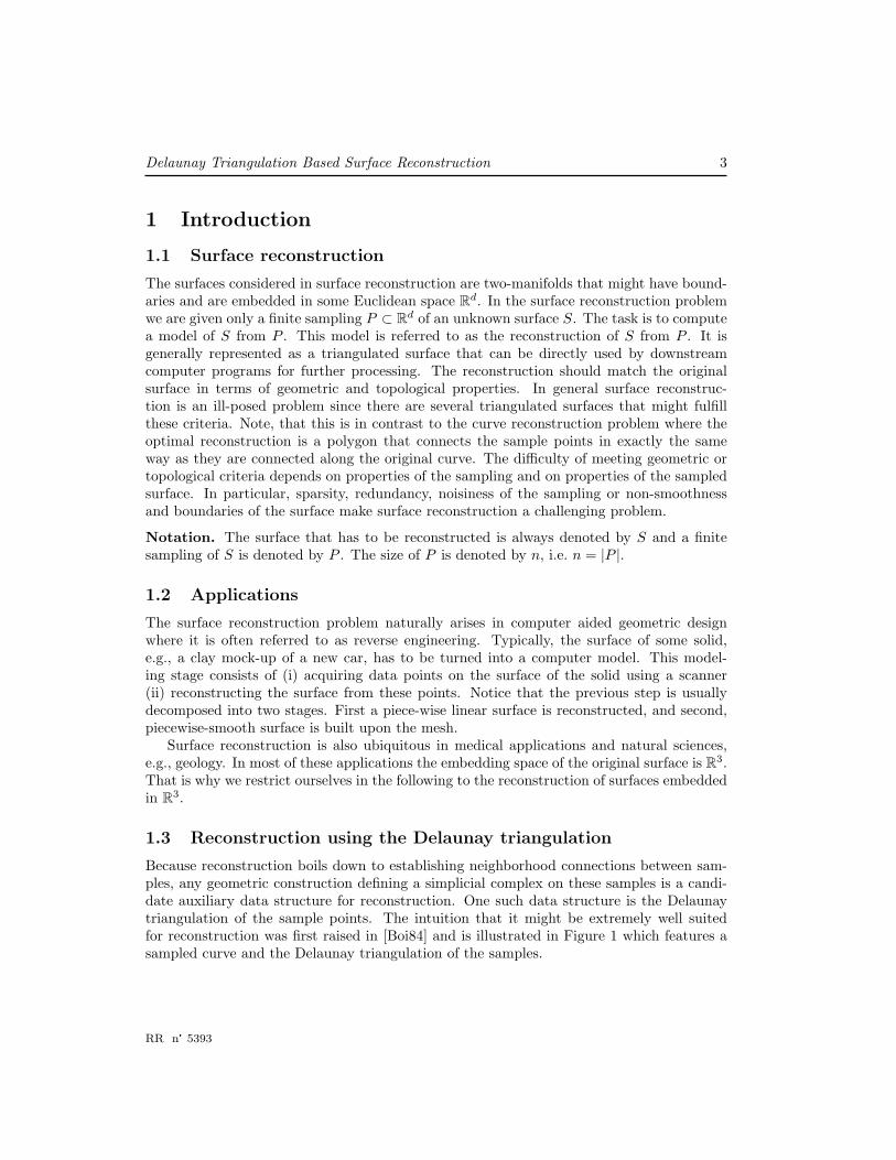
Because reconstruction boils down to establishing neighborhood connections between sam-ples, any geometric construction defining a simplicial complex on these samples is a candi-date auxiliary data structure for reconstruction. One such data structure is the Delaunaytriangulation of the sample points. The intuition that it might be extremely well suitedfor reconstruction was first raised in [Boi84] and is illustrated in Figure 1 which features asampled curve and the Delaunay triangulation of the samples.

RR n° 5393

4 Cazals & Giesen

Figure 1: Left: a sampled curve. Right: Delaunay contains a piece-wise linear approximationof the curve. Notice the Delaunay triangulation captures neighbors in all directions, nomatter how non-uniform the sampling.

The Delaunay triangulation is a cell complex that subdivides the convex hull of thesampling. If the sampling fulfills certain non-degeneracy conditions then all faces in theDelaunay triangulation are simplices and the Delaunay triangulation is unique. The combi-natorial and algorithmic complexity of the Delaunay triangulation grow exponentially withthe dimension of the embedding space of the original surface. In R3 the combinatorial as wellas the algorithmic complexity of the Delaunay triangulation is Θ(n2), where n = |P | is thesize of the sampling. However, it has been shown [ABL03] that the Delaunay triangulationof points that are well distributed on a smooth surface has complexity O(n log n). Robustand efficient methods to compute the Delaunay triangulation in R3 exist [cga]. Also impor-tant for the reconstruction problem is the Voronoi diagram which is dual to the Delaunaytriangulation. The Voronoi diagram subdivides the whole space into convex cells where eachcell is associated with exactly one sample point.

It seems that the Delaunay triangulation explores the neighborhood of a sample pointin all relevant directions in a way that even accommodates non-uniform samplings, see alsoFigure 1 for a two dimensional example.

There also approaches toward the surface reconstruction problem that are not based onthe Delaunay triangulation, e.g., level set methods [HOF01], radial basis function basedmethods [CBC+01] and moving least squares methods [ABCO+01]. That we do not coverthese approaches in this chapter does not mean that they are less suited or worse. Onthe practical side, many of them are very successfully applied in daily practice. On thetheoretical side though, these algorithms often involve non-local constructions making atheoretical analysis difficult. As opposed to these, algorithms elaborating upon Delaunayare more prone to such an analysis, and one of the goals of this survey is to outline the keygeometric features involved in these analysis.

INRIA

Delaunay Triangulation Based Surface Reconstruction 5

1.4 A classification of Delaunay based surface reconstruction meth-ods

Using the Delaunay triangulation still leaves room for quite different approaches to solvethe reconstruction problem. But all these approaches, that we sketch below, benefit fromthe structure of the Delaunay triangulation and the Voronoi diagram, respectively, of thesample points. We should note already here that many of the algorithms combine featuresof different approaches and as such are not easy to classify. We did the classification bywhat we consider the dominant idea behind a specific algorithm.

Tangent plane methods. If one considers a smooth surface with a sufficiently densesampling, the neighbors of a point in the point cloud should not deviate too much from thetangent plane of the surface at that point. It turns out that this tangent plane can be wellapproximated by exploiting the fact that under the condition of sufficiently dense samplingthe Voronoi cell of the sample point is elongated in the direction of the surface normal atthe sample point. This normal or tangent plane information, respectively, can be used toderive a local triangulation around each point.

Restricted Delaunay based methods. It is possible to define subcomplexes of theDelaunay triangulation by restricting it to some given subset of R3. Restricted Delaunaybased methods compute such a subset from the sampling. This subset should contain theunknown surface S provided the sampling is dense enough. The reconstruction basically isthe Delaunay triangulation of P restricted to the computed subset.

Inside / outside labeling. Given a closed surface S one can attempt to classify thetetrahedrons in the Delaunay triangulation as either inside or outside with respect to S. Theinterface between the inside and outside tetrahedrons should provide a good reconstructionof S. Algorithms that follow the inside / outside labeling paradigm often shell simplicesfrom the outside of the Delaunay triangulation of the sample points in order to discoverthe surface to be reconstructed. A subclass of the shelling algorithms guide the shelling bytopological information like the critical points of some function which can be derived fromthe sampling.

Empty balls methods. When reconstructing a surface, the simplices reported should belocal according to some definition. One such definition consists of requiring the existenceof a sphere that circumscribes the simplex and does not contain any sample point on itsbounded side. The ball bounded by such a sphere is called an empty ball. All Delaunaysimplices are local in this sense. This property can be used to filter simplices from theDelaunay triangulation, e.g., by considering the radii of the empty balls.

1.5 Organization of the chapter

The rest of this chapter is subdivided into two sections. Section 2 contains mathematical pre-requisites that are necessary to understand the ideas and guarantees behind the algorithmsthat are detailed in section 3.

RR n° 5393

6 Cazals & Giesen

2 Pre-requisites

2.1 Delaunay triangulations, Voronoi diagrams and related con-cepts

General position.

The sampling P is said to be in general position if there are no degeneracies of the followingkind: no three points on a common line, no four points on a common circle or hyperplaneand no five points on a common sphere. In the following we always assume that the samplingP is in general position. But note that the case that P is not in general position can also bedealt with algorithmically [EM90]. We make the general position assumption only to keepthe exposition simple.

Voronoi diagram.

The Voronoi diagram V (P ) of P is a cell decomposition of R3 in convex polyhedrons. EveryVoronoi cell corresponds to exactly one sample point and contains all points of R3 that donot have a smaller distance to any other sample point, i.e. the Voronoi cell correspondingto p ∈ P is given as follows

Vp = {x ∈ R3 : ∀q ∈ P ‖x− p‖ ≤ ‖x− q‖}.

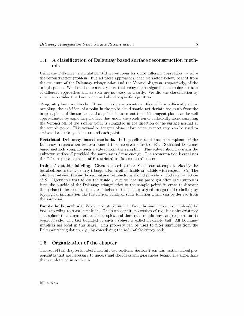
Closed facets shared by two Voronoi cells are called Voronoi facets, closed edges shared bythree Voronoi cells are called Voronoi edges and the points shared by four Voronoi cells arecalled Voronoi vertices. The term Voronoi object can denote either a Voronoi cell, facet,edge or vertex. The Voronoi diagram is the collection of all Voronoi objects. See Figure 2for a two-dimensional example of a Voronoi diagram.

Delaunay triangulation.

The Delaunay triangulation D(P ) of P is the dual of the Voronoi diagram, in the followingsense. Whenever a collection V1, . . . , Vk of Voronoi cells corresponding to point p1, . . . , pk

have a non-empty intersection, the simplex whose vertices are p1, . . . , pk belongs to theDelaunay triangulation. It is a simplicial complex that decomposes the convex hull of thepoints in P . That is, the convex hull of four points in P defines a Delaunay cell (tetrahedron)if the common intersection of the corresponding Voronoi cells is not empty. Analogously, theconvex hull of three or two points defines a Delaunay face or Delaunay edge, respectively,if the intersection of their corresponding Voronoi cells is not empty. Every point in P is aDelaunay vertex. The termDelaunay simplex can denote either a Delaunay cell, face, edgeor vertex. See Figure 2 for a two-dimensional example of a Delaunay triangulation.

INRIA

Delaunay Triangulation Based Surface Reconstruction 7

Figure 2: Voronoi and Delaunay diagrams in the plane

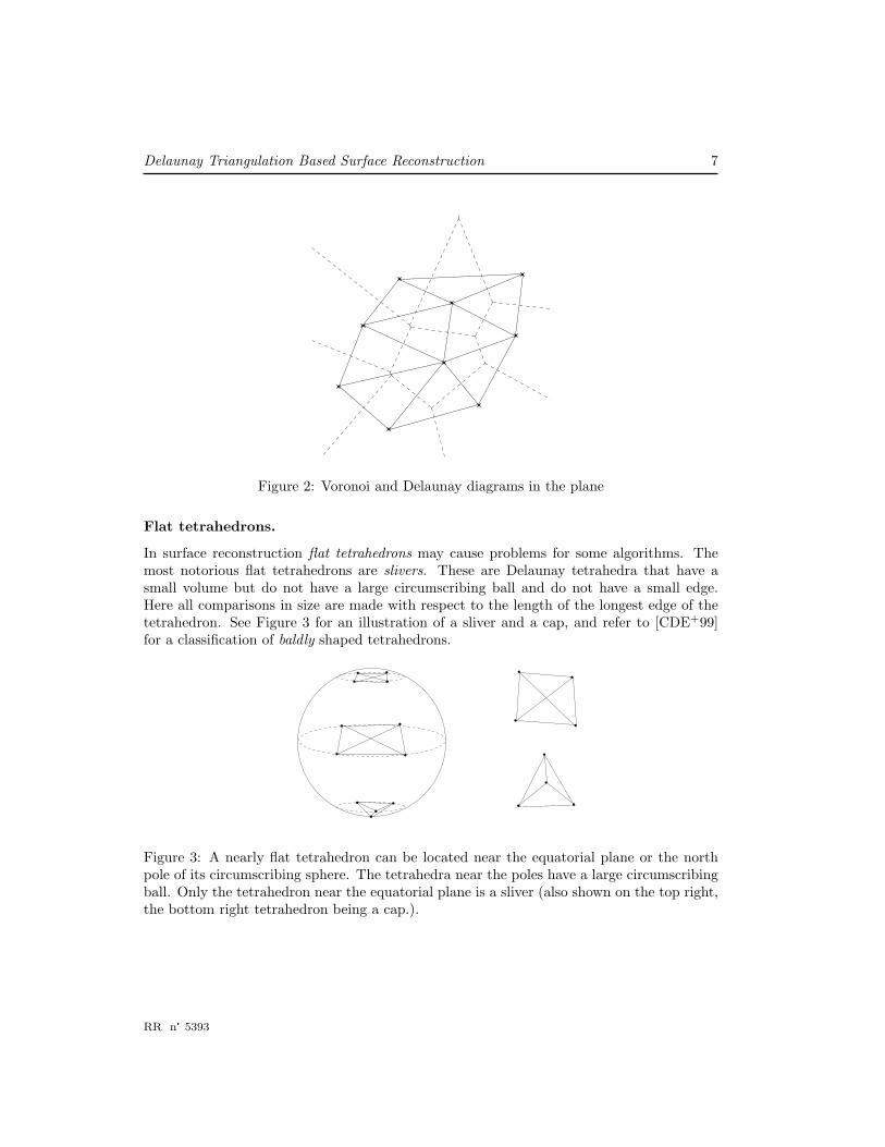
Flat tetrahedrons.

In surface reconstruction flat tetrahedrons may cause problems for some algorithms. Themost notorious flat tetrahedrons are slivers. These are Delaunay tetrahedra that have asmall volume but do not have a large circumscribing ball and do not have a small edge.Here all comparisons in size are made with respect to the length of the longest edge of thetetrahedron. See Figure 3 for an illustration of a sliver and a cap, and refer to [CDE+99]for a classification of baldly shaped tetrahedrons.

Figure 3: A nearly flat tetrahedron can be located near the equatorial plane or the northpole of its circumscribing sphere. The tetrahedra near the poles have a large circumscribingball. Only the tetrahedron near the equatorial plane is a sliver (also shown on the top right,the bottom right tetrahedron being a cap.).

RR n° 5393

8 Cazals & Giesen

Pole.

There are positive and negative poles associated with a Voronoi cell Vp. If Vp is bounded thenthe positive pole is the Voronoi vertex in Vp with the largest distance to the sample point p.Let u be the vector from p to the positive pole. If Vp is unbounded then there is no positivepole. In this case let u be a vector in the average direction of all unbounded Voronoi edgesincident to Vp. The negative pole is the Voronoi vertex v in Vp with the largest distance top such that the vector u and the vector from p to v make an angle larger than π/2.

Empty-ball property.

It follows from the definitions of Voronoi diagrams and Delaunay triangulations that therelative interior of a Voronoi object of dimension k, which is dual to a Delaunay object ofdimension 3 − k, consists of the set of points having exactly 3 − k + 1 nearest neighbors.Therefore, for any point in such a Voronoi object, there exists a ball empty of sample pointscontaining the vertices of the dual simplex on its boundary. The simplex is said to havethe empty ball property. See also Figure 4 for a two-dimensional example. For Delaunaytetrahedrons there is only one empty ball whereas there is a continuum of empty balls forDelaunay triangles and edges.

The empty ball property can be used to define sub-complexes of the Delaunay trian-gulation by imposing additional constraints on the empty balls. Here we discuss two suchrestrictions that lead to Gabriel simplices and α-shapes, respectively.

Gabriel simplex.

A simplex is called Gabriel if its smallest circumscribing ball is empty. Obviously all Gabrielsimplices are contained in the Delaunay triangulation. Gabriel simplices also have a dualcharacterization: a Delaunay simplex is Gabriel iff its dual Voronoi object intersects theaffine hull of the simplex.

Well known and heavily used is the Gabriel graph which is the geometric graph thatcontains all one dimensional Gabriel simplices.

α-shape.

Following the previous discussion, one can attach to each simplex of a Delaunay triangulationan interval of positive real numbers corresponding to the radii of empty balls centered on theVoronoi object dual of the simplex. We refer to this interval as the interval of the simplex.Given a positive real number α, a simplex of dimension k < 3 is called α-exposed if itsinterval contains α. The set of α-exposed simplices defines the α-shape of the point set. Anα-shape usually contains simplices of dimensions between zero and two.

INRIA

Delaunay Triangulation Based Surface Reconstruction 9

� �� �

� �

� �

� �

� �

Figure 4: Empty balls centered on Voronoi objects

�

�

�

�

�

Figure 5: All edges but edge ab are Gabriel edges

RR n° 5393

10 Cazals & Giesen

If we let α grow starting from 0, every Delaunay simplex of dimension smaller than threeappears in the evolving α-shape at the lower end of its interval and eventually disappears atthe upper end of its interval. Another geometric characterization of the points of appearanceand disappearance is as follows: Let balls grow at the sample points with uniform speed. Asimplex appears in the α-shape, where α is the evolving radius of the growing balls, whenthe balls corresponding to the vertices of the simplex intersect for the first time. Note thatthis intersection happens on the dual Voronoi object of this simplex. It disappears whenthe common intersection of the balls corresponding to the vertices of the simplex completelycontains the dual Voronoi object of the simplex. This growing process is illustrated inFigure 6

Note that α can be interpreted as a spatial scale parameter. If P is a uniform samplingof the surface S then there exist α-values such that the corresponding α-shapes of P providea reasonable reconstruction of S.

One can also use restricted diagrams that we are going to introduce now to describe anevolving sub-complex of the Delaunay triangulation very similar to α-shapes. Actually thesimilarity is such that one also refers to these sub-complexes as α-shapes.

Restricted Voronoi diagram and restricted Delaunay triangulation.

Given a subset X ⊂ R3. We can restrict the Voronoi diagram of P to to X by replacing ev-ery Voronoi object with its intersection with X. The restricted Voronoi diagram is denotedas VX(P ). The Delaunay triangulation DX(P ) of P restricted to X is defined similarly asthe Delaunay triangulation of P . The only difference is that instead of taking the com-mon intersection of Voronoi cells now the common intersection of restricted Voronoi cells istaken. That is, whenever a collection V1 ∩X, . . . , Vk ∩X of Voronoi cells corresponding topoint p1, . . . , pk restricted to X have a non-empty intersection, the simplex whose verticesare p1, . . . , pk belongs to the restricted Delaunay triangulation. The restricted Delaunaytriangulation of a plane curve is illustrated in Figure 7.

The Delaunay triangulation restricted to a set of balls with radius α centered at thesample points is called the α-complex. The boundary of the α-complex is the α-shape, andthe α value of appearance of Delaunay simplices (of dimension 0 to d − 1) is the same asfor α-shapes. Phrased differently, the differences between the α-complex and the α-shapeare twofold: first, once a simplex appears in the α-complex, it stays forever; second, theα-complex also contains Delaunay tetrahedra.

Closed ball property.

The restricted Voronoi diagram VS(P ) of a sampling P of a surface S has the closed ballproperty if the intersection of S with every Voronoi object in V (P ) is homeomorphic to aclosed ball whose dimension one smaller then that of the Voronoi object. (Notice that the

INRIA

Delaunay Triangulation Based Surface Reconstruction 11

Figure 6: α-complex and α-shapes at two successive times. for each Fig.: the main Fig. andthe reduced Fig. feature the α-complex and α-shape

Figure 7: Diagrams restricted to a curve

Figure 8: Triangulation restricted to a surface

RR n° 5393

12 Cazals & Giesen

transverse intersection of a Voronoi cell of dimension k with a manifold of dimension d− 1has dimension equal to k + (d − 1) − d = k − 1.) Edelsbrunner and Shah [ES97] were ableto relate the topology of the restricted Delaunay triangulation DS(P ) to the topology of S.

Theorem 1 Let S be a surface and P be a sampling of S such that VS(P ) has the closedall property. Then DS(P ) and S are homeomorphic.

Power diagram and regular triangulation.

The concepts of Voronoi- and Delaunay diagrams are easily generalized to sets of weightedpoints. A weighted point p in R3 is a tuple (z, r) where z ∈ R3 denotes the point itself andr ∈ R its weight. Every weighted point gives rise to a distance function, namely the powerdistance function,

πp : R3 → R, x 7→ ‖x− z‖2 − r.

Let P now be a set of weighted point in R3. The power diagram of P is a decompositionof R3 into the power cells of the points in P . The power cell of p ∈ P is given as

Vp = {x ∈ R3 : ∀q ∈ P, πp(x) ≤ πq(x)}.

The points that have the same power distance from two weighted points in P form a hy-perplane. Thus Vp is either a convex polyhedron or empty. Closed facets shared by twopower cells are called power facets, closed edges shared by three power cells are called poweredges and the points shared by four power cells are called power vertices. The term powerobject can denote either a power cell, facet, edge or vertex. The power diagram of P is thecollection of all power objects.

The dual of the power diagram of P is called the regular triangulation of P . The dualityis defined in exactly the same way as for Voronoi diagrams and Delaunay triangulations.That is why regular triangulations are also referred to as weighted Delaunay triangulations.

Natural Neighbors.

Given a Delaunay triangulation, it is natural to define the neighborhood of a vertex as theset of vertices this vertex is connected to. This information is of combinatorial nature andcan be made quantitative using the so-called natural coordinates which were introduced bySibson [Sib81].

Given a point x ∈ R3 which is not a sample point, define V +(P ) = V (P ∪{x}), D+(P ) =D(P ∪ {x}), and denote by V +

x the Voronoi cell of x in V +(P ). In addition, for any samplepoint p ∈ P define V(x,p) = V +

x ∩ Vp and denote by wp(x) the volume of V(x,p). The naturalneighbors of a point x are the the sample points in P that are connected to x in D+(P ).Equivalently, these are the points p ∈ P for which V(x,p) 6= ∅. The natural coordinate

INRIA

Delaunay Triangulation Based Surface Reconstruction 13

� �

� �

� �

� �

� �

� �

�

Figure 9: Point x has six natural neighbors

a

b

c

d

x1x2

x3

Figure 10: Critical points of the distance function. Points x1, x2 are regular, but point x3

is critical.

associated with a natural neighbor is the quantity

λp(x) =wp(x)w(x)

, with w(x) =∑p∈P

wp(x). (1)

For an illustration of these definitions see Figure 9.

The term coordinate is clearly evocative of barycentric coordinates. Recall that in anythree-dimensional affine space, a set of four linearly independent points pi, i = 1, . . . , 4define a basis of the affine space. Moreover, every point x decomposes uniquely as x =∑

i=1,...,4 λpi(x)pi, with λpi

(x) the barycentric coordinate of x wrt pi. Natural coordinatesprovide an elegant extension of barycentric coordinates to the case where one has more than

RR n° 5393

14 Cazals & Giesen

four linearly points. The following results have been proven in a number of ways [Sib81,Aur88, Bro97, HS02].

Theorem 2 The natural coordinates satisfy the requirements of a coordinate system, namely,

(1) for any p ∈ P , λp(q) = δpq where δpq is the Kronecker symbol and

(2) the point x is the weighted center of mass of its neighbors. That is,

x =∑p∈P

λp(x) p, with∑p∈P

λp(x) = 1. (2)

Induced distance function.

Voronoi diagrams of a sampling P are closely related to the distance function

h : R3 → R, x 7→ minp∈P

‖x− p‖

induced by the set of sample points. This distance function is smooth everywhere besidesat the points in P and on the lower dimensional Voronoi objects, i.e. on the facets, edgesand vertices.

At every point x inside a Voronoi region, the gradient of h is the unit vector pointedaway from the center of the region. Interestingly, for points x on lower dimensional Voronoiobjects, one can in general define a generalized gradient, as depicted on Fig. 10. Let xbe a point and denote C(x) the nearest points of x —C(x) consists of the vertices dual ofthe Voronoi object containing x. If x does not belong to the convex hull of C(x), then thegeneralized gradient of x points away from the affine hull of C(x). On the other hand, if xbelongs to C(x), it is locally impossible to move x so as to increase h, and point x is calleda critical point.

It was was observed by Edelsbrunner [Ede04] and later proved by Giesen and John [GJ03]that the critical points of the distance function, i.e., the local extrema and the saddle points,can be characterized in terms of Delaunay simplices and Voronoi objects.

Theorem 3 The critical points of h are the intersection points of Voronoi objects and theirdual Delaunay simplices. The local maxima are Voronoi vertices contained in their dualDelaunay cell. The saddle points are intersection points of Voronoi facets and their dualDelaunay edges and intersection points of Voronoi edges and their dual Delaunay triangles.All sample points are minima.

The index of a critical point is the dimension of the Delaunay simplex involved in itsdefinition. See Figure 2.1 for an example in two dimensions.

INRIA

Delaunay Triangulation Based Surface Reconstruction 15

Induced flow and stable manifolds.

As in the case of smooth functions there is a unique direction of steepest ascent of h at everynon-critical point of h. Assigning to the critical points of h the zero vector and to everyother point in R3 the unique unit vector of steepest ascent defines a vector field on R3. Thisvector field is non smooth but nevertheless gives rise to a flow on R3, i.e., a mapping

φ : [0,∞)× R3 → R3,

such that at every point (t, x) ∈ [0,∞)× R3 the right derivative

limt←t′

φ(t, x)− φ(t′, x)t− t′

exists and is equal to the unique unit vector of steepest ascent at x. The flow basically tellshow a point would move if it would always follow the steepest ascent of the distance functionh. The curve that a point x follows is given by φx : R → R3, t 7→ φ(t, x) and called the orbitof x. See Figure 2.1 for some example orbits in two dimensions.

Given a critical point x of h the set of all points whose orbit ends in x, i.e. the set ofall points that flow into x, is called the stable manifold of x. The collection of all stablemanifolds forms a cell complex which is called flow complex. See Figure 2.1 for examples ofstable manifolds in two dimensions.

2.2 Medial axis and derived concepts

Medial axis.

The medial axis M(S) of a closed subset S ⊂ R3 consists of all points in R3\S havingtwo or more nearest points on S. In a way the medial axis generalizes the concept of theVoronoi diagram of a point set. We have seen when discussing the empty ball property thatthe Voronoi objects of dimension k with k = 0, . . . , 2 consist of all points equidistant from3− k + 1 sample points.

Smooth surfaces S play a special role in reconstruction since for their reconstructionseveral guarantees can be provided under a certain sampling condition. This samplingcondition is based on the medial axis of S that is why we here provide some more details onthe structure of the medial axis of a smooth surface S.

Structure of the medial axis of a smooth surface.

The medial axis of a smooth surface S shares another structural property with the Voronoidiagram of a finite point set, namely, it has a stratified structure. For Voronoi diagram thisstructure means that a Voronoi facet is the common intersection of two Voronoi regions, aVoronoi edge is the common intersection of three Voronoi facets and a Voronoi vertex is thecommon intersection of four Voronoi edges. To precisely describe the stratified structure of

RR n° 5393

16 Cazals & Giesen

Figure 11: From the left: 1) The local minima , saddle points � and local maxima ⊕ ofthe distance function induced by the sample points (local minima). 2) Some orbits of theflow induced by the sample points. 3) The stable manifolds of the saddle points. 4) Thestable manifolds of the local maxima.

INRIA

Delaunay Triangulation Based Surface Reconstruction 17

M(S), one needs the notion of contact between a sphere and the surface. Informally, thecontact of a sphere at a point p of S tells how much the sphere and the surface agree at p.More precisely, an A1 contact means that the tangent plane to the sphere and to S agree atp; an A2 contact point has the property of an A1 point with the additional property that theradius of the sphere is the inverse of a principal curvature of S at p; at last, an A3 contactis like an A2 contact with the additional property that the curvature involved is an extremealong the corresponding line of curvature. Focusing on the centers of the contact spheresrather than the contact points themselves, and denoting Ak

1 a set of k ≥ 1 simultaneous A1

contacts between a sphere and the surface, the structure of the M(S) is described by thefollowing theorem [Yom81, GK00] which is illustrated by an example in Figure 12.

Theorem 4 The medial axis of a smooth surface S in R3 is a stratified variety containingsheets, curves and points. The sheets correspond to A2

1 contacts, the curves to A31 and

A3 contacts, and the points to A41 and A3A1 contacts. Moreover, one has the following

incidences. At an A41 point, six A1

2 sheets and four A31 curves meet. Along an A3

1 curve,three A2

1 sheets meet. A3 curves bound A21 sheets. At last, the point where an A2

1 sheetvanishes is an A3A1 point.

Medial axis transform.

A concept closely related to the medial axis of a closed subset S ⊂ R3 is the skeleton ofR3\S, which consists of the centers of maximal spheres included in R3\S. Here maximal ismeant with respect to inclusion among spheres. For a smooth surface S the closure of themedial axis is actually equal to the skeleton of R3\S. The medial axis transform builds onthe close relationship of the skeleton and the medial axis, namely, the medial axis transformis the collection of maximal empty balls centered at the medial axis of S. It can be shownthat a smooth surface S can be recovered as the envelope of its medial axis transform.

Tubular neighborhoods.

A natural tool involved in the analysis of several reconstruction algorithms is that of tubularneighborhood or tube of a surface S. As subsumed by the name, a tube of a surface is athickening of the surface such that within the volume of the thickening, the projection of apoint x to the nearest point π(x) on S remains well defined. Following our discussion of themedial axis, a surface can always be thickened provided the thickening avoids the medialaxis. Moreover, it is easily checked that the projection onto S proceeds along the normalat the projection point. This property provides a way to retract the neighborhood onto thesurface.

Feature size.

The feature size is a function f : S → R on the surface S that assigns to each point in S itsleast distance to the medial axis of S. An immediate consequence of the triangle inequality is

RR n° 5393

18 Cazals & Giesen

� ��

� ��

� ��

� �

��

� �

� ��� �

� ��

� ��

�� � ��

� ��

��

�

Figure 12: The stratified structure of the medial axis of a smooth surface

INRIA

Delaunay Triangulation Based Surface Reconstruction 19

�

� �

�

� �

� � � � � � � � � � � � � � � � � � � � � � � � � � � � � � � � � � � � � � � � �

Figure 13: The feature size is 1-Lipschitz

�� �

� �

� � �

Figure 14: For a non-smooth curve, some Voronoi centers may not converge to the medialaxis.

that the feature size of smooth surface is Lipschitz continuous with Lipschitz constant 1, seeFigure 13 for an illustration. The feature size can be used to establish another quantitativeconnection of a surface and its medial axis [BC01b] by using the following theorem.

Theorem 5 Let B be a ball centered at x ∈ R3 with radius r that intersects the surface S.If this intersection is not a topological ball then B contains a point of the medial axis of S.

¿From this theorem we can conclude that any ball centered at any point p ∈ S whoseradius is smaller then the feature size f(p) at p intersects S in a topological disk.

ε-sampling.

Amenta and Bern [ABE98, AB99] introduced a non-uniform measure of sampling densityusing the feature size. For ε > 0 a sampling P of a surface S is called an ε-sampling of S ifevery point x on S has a point of P in distance at most εf(x).

We next provide three theorems that involve ε-samples. The first theorem is concernedwith the topological equivalence of the restricted Delaunay triangulation DS(P ) and a sur-face S for an ε-sample P . The second theorem is concerned with the convergence of Voronoi

RR n° 5393

20 Cazals & Giesen

vertices of the Voronoi diagram of an ε-sample of a smooth surface S towards the medialaxis M(S) of S. The last theorem provides a good approximation of the normal of S atsome sample point in an ε-sample P .

Amenta and Bern [AB99] proved the following theorem, which provides a topologicalguarantee for a value of ε less than ∼ 0.3. In the context of surface reconstruction, thisTheorem should be put in perspective wrt Theorem 1:

Theorem 6 If P is an ε-sample of S such that ε satisfies

cos(

arcsin(

2ε

1− ε

)+

ε

1− 3ε

)>

ε

1− ε

then VS(P ) has the closed ball property.

It can be shown that the Voronoi vertices of a dense sampling of a planar smooth curvelie close to the medial axis of the curve. This result is false in general for non smooth curves,as illustrated in Figure 14. It is also false in general for dense samplings of smooth surfaces.In fact for any point x ∈ R3\S, there exists an arbitrarily dense sampling P of S such thatx is a Voronoi vertex of V (P ) provided some non-degeneracy holds. To see this grow a ballaround x until it touches S. Now grow it a little bit further and put four sample points onthe intersection of S with the boundary of the ball. Then x is shared by the Voronoi cellsof the four points, i.e., it is a Voronoi vertex if the four points are in general position.

Fortunately, it was observed by Amenta and Bern [AB99] that the poles of the Voronoidiagram of a sampling of a smooth surface converge to the medial axis.

Theorem 7 Let P be an ε-sample of a smooth surface S the poles of the Voronoi diagramV (P ) converge to the medial axis M(S) of S as ε goes to zero.

Finally, also the following theorem is due to Amenta and Bern [AB99]. It follows fromTheorem 7.

Theorem 8 Let P be an ε-sample of a smooth surface S. For any sample point p ∈ P letp+ be the pole of the Voronoi cell Vp. The angle between the normal of S at p and the the

vector p− p+ if oriented properly can be bounded by arcsin(

2ε1−ε

).

2.3 Topological and geometric equivalences

To assess the quality of a reconstruction we need topological and geometric concepts.

Topological concepts.

Homeomorphy. Two surfaces are called homeomorphic if there is a homeomorphism be-tween them. A homeomorphism is a continuous bijection of one surface onto the other, suchthat the inverse is also continuous. Two homeomorphic surfaces have the same properties

INRIA

Delaunay Triangulation Based Surface Reconstruction 21

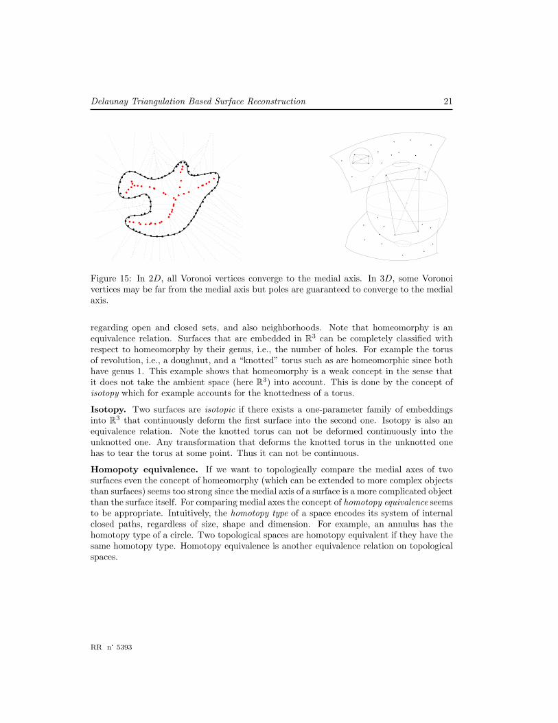
Figure 15: In 2D, all Voronoi vertices converge to the medial axis. In 3D, some Voronoivertices may be far from the medial axis but poles are guaranteed to converge to the medialaxis.

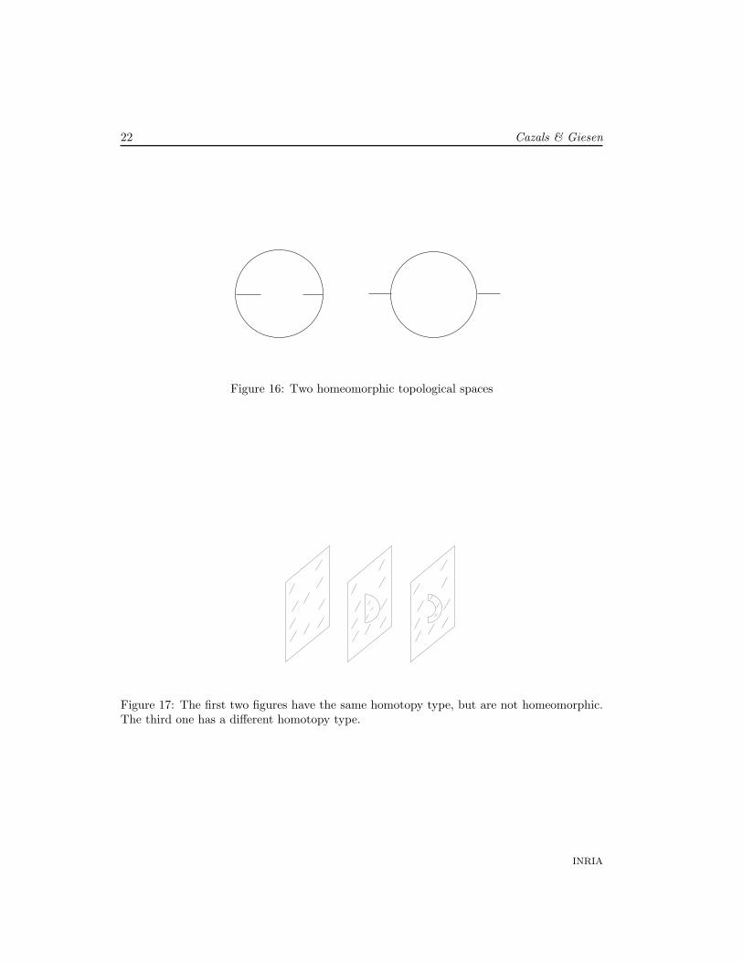
regarding open and closed sets, and also neighborhoods. Note that homeomorphy is anequivalence relation. Surfaces that are embedded in R3 can be completely classified withrespect to homeomorphy by their genus, i.e., the number of holes. For example the torusof revolution, i.e., a doughnut, and a “knotted” torus such as are homeomorphic since bothhave genus 1. This example shows that homeomorphy is a weak concept in the sense thatit does not take the ambient space (here R3) into account. This is done by the concept ofisotopy which for example accounts for the knottedness of a torus.

Isotopy. Two surfaces are isotopic if there exists a one-parameter family of embeddingsinto R3 that continuously deform the first surface into the second one. Isotopy is also anequivalence relation. Note the knotted torus can not be deformed continuously into theunknotted one. Any transformation that deforms the knotted torus in the unknotted onehas to tear the torus at some point. Thus it can not be continuous.

Homopoty equivalence. If we want to topologically compare the medial axes of twosurfaces even the concept of homeomorphy (which can be extended to more complex objectsthan surfaces) seems too strong since the medial axis of a surface is a more complicated objectthan the surface itself. For comparing medial axes the concept of homotopy equivalence seemsto be appropriate. Intuitively, the homotopy type of a space encodes its system of internalclosed paths, regardless of size, shape and dimension. For example, an annulus has thehomotopy type of a circle. Two topological spaces are homotopy equivalent if they have thesame homotopy type. Homotopy equivalence is another equivalence relation on topologicalspaces.

RR n° 5393

22 Cazals & Giesen

Figure 16: Two homeomorphic topological spaces

Figure 17: The first two figures have the same homotopy type, but are not homeomorphic.The third one has a different homotopy type.

INRIA

Delaunay Triangulation Based Surface Reconstruction 23

��

�

� �

�

� � � � � � � � �� � � � � � � �

Figure 18: The one-sided Hausdorff distance is not symmetric

Geometric concepts.

Hausdorff distance. The Hausdorff distance is a measure for the distance of two subsetsof some metric space. We are interested in the case where these subsets are surfaces ormedial axes of surfaces in R3.

Given two closed subsets X, Y of R3, define the one-sided Hausdorff distance h(X, Y )as h(X, Y ) = maxx∈X miny∈Y ‖x − y‖. The one-sided Hausdorff distance is not a distancemeasure since in general it is not symmetric. Symmetrizing h yields the Hausdorff distancedefined by H(X, Y ) = max{h(X, Y ), h(Y, X)}. See also Figure 18.Normals and tangent planes. Given two surfaces, their Hausdorff distance just takes intoaccount their relative positions. In the context of surface reconstruction, we shall also beinterested in differential properties of the reconstructed surface with respect to the sampledsurface. At the first order, such a measure is provided by the tangent planes (or the normals)to the surfaces, a quantity known to play a key role in the definition of metric properties ofsurfaces [MT02].

3 Overview of the algorithms

3.1 Tangent plane based methods

We assume the the sampled surface S is smooth, i.e. there exists a well defined tangentplane at each point of the surface. Since we only deal with surfaces of co-dimension one,i.e. surfaces embedded in R3, approximating the tangent plane at some point of the surfaceis equivalent to approximating the normal at this point. Thus here tangent plane basedmethods include normal based methods. The first algorithm based on the tangent planes atthe sample points is Boissonnat’s [Boi84] algorithm. It probably is the first algorithm at alldesigned to solve the surface reconstruction problem. Simply put, this algorithm reduces thereconstruction problem to the computation of local reconstructions in the tangent planes atthe sample points. These local reconstructions have to be pasted together in the end.

RR n° 5393

24 Cazals & Giesen

Lower Dimensional Localized Delaunay Triangulation.

Gopi, Krishan and Silva [GKS00] designed an algorithm that is very similar in nature toBoissonnat’s early algorithm.

. Bottom-line. This algorithm has three major steps. First, normal and tangent planeapproximation at the sample points. Second, selection of a neighborhood of sample pointsfor each sample point. Third, projection of the neighborhood of a sample point on its tangentplane and computation of the Delaunay neighborhood of the sample point in its projectedneighborhood. Sample points p, q, r ∈ P form a triangle in the reconstruction if they all aremutually contained in their Delaunay neighborhoods.

. Algorithm. The normal and tangent plane approximation at the sample points is doneusing the eigenvectors of the covariance matrix of the k nearest neighbors of the samplepoint p. The covariance matrix is the 3× 3 matrix

C =∑

i

(qi − p)(qi − p)T

where the sum is taken over the k nearest neighbors of p in P and p is the centroid ofthe k nearest neighbors of p. The eigenvector corresponding to the smallest eigenvalue ofthe positive definite, symmetric matrix C is taken as the approximate normal at p. Theremaining two eigenvectors span an approximate tangent plane at p. The approximatenormals at the sample points are consistently oriented by propagating the orientation atsome seed sample point along the edges of the Euclidean minimum spanning tree of P .

¿From the approximated normals at the sample points the directional normal variationsand even the principal curvatures at the sample points can be estimated using again the knearest neighbors of the sample points. The approximated principal curvatures kmin(p) andkmax(p) at a sample point p are used to locally approximate the unknown surface S by aheight function

h(r, θ) =r2

2(kmin(p) cos2 θ + kmax(p) sin2 θ)

parameterized by polar coordinates r and θ over the approximated tangent plane at p.The neighborhood of a sample point p contains all sample points in P at distance at most2kmax(p)/kmin(p) from p whose height value is bounded by some function of kmin(p).

The neighbors of a sample point p are projected onto the approximated tangent planeat p by rotating the vector from p to its neighbor into the tangent plane. In the tangentplane the Delaunay neighbors of p are determined by computing a two dimensional Delaunaytriangulation of p and its projected neighbors. The output of the algorithm consists of alltriangles with vertices in P whose vertices are mutual Delaunay neighbors.

. Complexity. The complexity of the algorithm was not theoretically analyzed. But isseems reasonable to assume that the local operations at each sample point can be done inconstant time each which would amount to a linear time complexity in total. But thereare also the global operations of determining the neighborhoods of the sample points and of

INRIA

Delaunay Triangulation Based Surface Reconstruction 25

consistently orienting the normals. Though the latter operation is not really needed for thealgorithm to work.

. Guarantees. The triangles output by the algorithm form surface homeomorphic toS provided a curvature based, locally uniform sampling condition holds. This samplingcondition also takes care of different parts of S coming close together.

. Extensions. Some heuristics are given to deal with samplings that do not fulfill thesampling condition. Especially the case of under-sampling is dealt with, though even theextensions do not make sure that the output is topological surface in practice. Of coursealso oversampling can cause problems since at some points of the algorithm the k nearestneighbors of a sample point are used. This k neighborhood can be spatially biased in thecase of oversampling. This bias can invalidate the geometric approximations of normals,tangent planes and curvatures.

Greedy algorithm.

The Greedy algorithm was introduced by Cohen-Steiner and Da in [CSD04]. It incrementallygrows a surface from a seed triangle guided by the intuition that the normals vary smoothlyover the surface S.

. Bottom-line. The greedy algorithm incrementally reconstructs an oriented surface S byselecting triangles out of the Delaunay triangulation D(P ) of P and stitching them to S.The guideline for the selection is straightforward: the incremental construction should makeeasy decisions first by stitching triangles which do not yield ambiguities.

. Algorithm. When extending the surface, a valid triangle is a triangle whose stitchingdoes not create a topological singularity, and admissible glue operations are of four typesextension, gluing, hole filing, ear filling.

Let e be a boundary edge of S. Out of all the valid triangles t incident to e, one of themis chosen as candidate for the surface extension. To define the candidate, denote rt theradius of the smallest empty ball circumscribing a triangle t. Among all the triangles whosedihedral angle βt across e is less than some threshold αs (an angle near π), the candidate isthe triangle with least rt. Since a greedy approach is used, one needs to grade the differentcandidates. To do so, each triangle is assigned a grade which is 1/rt if βt is less than athreshold β, and −βt otherwise.The threshold αs prevents from considering facets whose stitching would cause a fold-overabout a large dihedral angle. Notice also the grading strategy favors small triangles providedthe dihedral angle is less than the threshold β.

Equipped with these notions, the algorithm consists of the initialization and extensionstages. First, the triangle with least circumradius is chosen as a seed, and its edges arepushed into a priority queue Q. Next, the algorithm iterates over Q and processes trianglesin order of decreasing confidence. Once a candidate triangle has been popped, a checkis performed to see whether a possible extension is possible. This might not be the case

RR n° 5393

26 Cazals & Giesen

anymore due to potential changes in the environment of the triangle. In any case, thepriority queue and the surface are updated.

By construction, the output of the Greedy algorithm is a triangulated and orientedsurface, which may not interpolate all the samples since the used thresholds might leavesome sample points without incident triangle.

. Complexity. The algorithm uses the Delaunay triangulation of the samples togetherwith the priority queue. Both data structures determine the complexity of the algorithm.

. Guarantees. No guarantee can be provided on the quality of the reconstruction due to thedifficulty of handling clusters of flat tetrahedrons. As the surface extension is incremental,such clusters can be approached in various manners from different directions, thus makingit impossible to close the surface.

. Extensions. Two heuristics are used to accommodate boundaries as well as sharp fea-tures. For boundaries, a candidate triangle is discarded as soon as the radius of its emptyball is significantly larger than that of the triangle it would be stitched to. Sharp edgesare detected and removed through the removal of samples which are not part of the outputsurface.

3.2 Restricted Delaunay based methods

Since all Delaunay based surface reconstruction algorithms filter out a subset of the Delau-nay triangulation D(P ) of the sampling P it seems natural and very appealing to choose justthese simplices from D(P ) that are restricted to some subset of R3 that is a good approxi-mation of the unknown surface S and can be computed efficiently from P . This paradigm ismotivated by the fact that if we could directly compute the Delaunay triangulation DS(P )of P restricted to S we would be done since due to the theorems of Edelsbrunner andShah (Theorem 1) and Amenta and Bern (Theorem 6), respectively, for sufficiently denseε-samples DS(P ) is homeomorphic to S.

Crust.

The Crust algorithm was designed by Bern and Amenta [AB99] who also were the first toprovide detailed guarantees for the reconstruction provided some ε-sampling condition isfulfilled.

. Bottom-line. The Crust is based on the Delaunay triangulation D(P ∪Q) of P and theset Q of poles of the Voronoi diagram V (P ). Let V be the union of the Voronoi cells ofthe points in P in the Voronoi diagram V (P ∪Q) of P ∪Q. In a nutshell the Crust is theDelaunay triangulation of P restricted to V . The rationale behind this is that R3 \V shouldcover the medial axis M(S) of the surface S. Thus restricting the Delaunay triangulationof P to V should remove all simplices from D(P ) that cross the medial axis M(S) ofS. On the other hand V should provide a thickened version of S and thus the restricted

INRIA

Delaunay Triangulation Based Surface Reconstruction 27

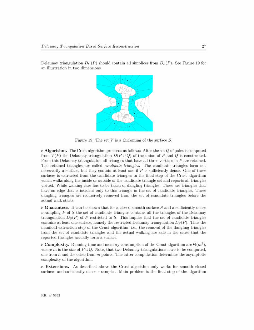
Delaunay triangulation DV (P ) should contain all simplices from DS(P ). See Figure 19 foran illustration in two dimensions.

Figure 19: The set V is a thickening of the surface S.

. Algorithm. The Crust algorithm proceeds as follows: After the set Q of poles is computedfrom V (P ) the Delaunay triangulation D(P ∪ Q) of the union of P and Q is constructed.From this Delaunay triangulation all triangles that have all three vertices in P are retained.The retained triangles are called candidate triangles. The candidate triangles form notnecessarily a surface, but they contain at least one if P is sufficiently dense. One of thesesurfaces is extracted from the candidate triangles in the final step of the Crust algorithmwhich walks along the inside or outside of the candidate triangle set and reports all trianglesvisited. While walking care has to be taken of dangling triangles. These are triangles thathave an edge that is incident only to this triangle in the set of candidate triangles. Thesedangling triangles are recursively removed from the set of candidate triangles before theactual walk starts.

. Guarantees. It can be shown that for a closed smooth surface S and a sufficiently denseε-sampling P of S the set of candidate triangles contains all the triangles of the Delaunaytriangulation DS(P ) of P restricted to S. This implies that the set of candidate trianglescontains at least one surface, namely the restricted Delaunay triangulation DS(P ). Thus themanifold extraction step of the Crust algorithm, i.e., the removal of the dangling trianglesfrom the set of candidate triangles and the actual walking are safe in the sense that thereported triangles actually form a surface.

. Complexity. Running time and memory consumption of the Crust algorithm are Θ(m2),where m is the size of P ∪Q. Note, that two Delaunay triangulations have to be computed,one from n and the other from m points. The latter computation determines the asymptoticcomplexity of the algorithm.

. Extensions. As described above the Crust algorithm only works for smooth closedsurfaces and sufficiently dense ε-samples. Main problem is the final step of the algorithm

RR n° 5393

28 Cazals & Giesen

that extracts a surfaces from the set of candidate triangles. For practical data sets thatdo not fulfill the requirements of the algorithm it can happen that this last step removesalmost all candidate triangles since dangling triangles are removed recursively. This can beprevented if the removal of the dangling triangles is implemented in a more conservativefashion. This done the Crust algorithm can also cope with surfaces with boundaries and a“certain amount of non-smoothness” in practice.

Cocone.

The Cocone algorithm was designed by Amenta et al. [ACDL00] as a successor and improve-ment of the Crust algorithm.

. Bottom-line. The Cocone algorithm builds as the Crust algorithm on the idea of ap-proximating the Delaunay triangulation DS(P ) of P restricted to S by computing a subsetC ⊂ R3 from P which is a thickened version of S such that the Delaunay triangulationDC(P ) of P restricted to C can computed. The subset C is defined as follows: For everysample point p ∈ P approximate the normal of S at p using the pole of the Voronoi cell Vp

in V (P ), see Theorem 8. The co-cone at p is now defined as the intersection of Vp with thecomplement of a double cone with apex p and fixed opening angle around the approximatenormal at p, see Figure 20 for a two dimensional example. The set C is the union of all suchco-cones. Note, that C can be computed just from P . Theorem 7 implies that the localthickening of S using co-cones is small compared to the local feature size and thus C is areasonable approximation of S.

Figure 20: The co-cone of a sample on a curve together with the Voronoi cell of the samplepoint and its pole.

INRIA

Delaunay Triangulation Based Surface Reconstruction 29

Figure 21: Balls of opposite (the same) color intersect shallowly (deeply)

. Algorithm. As the Crust algorithm the Cocone algorithm first computes a subset ofcandidate triangles from the triangles in D(P ). A triangle t in D(P ) is a candidate triangleif its dual Voronoi edge e intersects any of the co-cones. This intersection test boils down togo through the vertices of t and check if e intersects the co-cone of one of the vertices whichis checking the angles the of vectors from a vertex v incident to t to the endpoints of e withthe approximate normal at v. As for the Crust algorithm the candidate triangles form notnecessarily a surface, but they contain at least one if P is sufficiently dense. Finally, the laststep of the Crust algorithm is used to extract one of these surfaces.

. Guarantees. The same guarantees as for the Crust algorithm hold under the sameconditions.

. Complexity. The running time and memory consumption of the Cocone algorithm isΘ(n2) where n is the size of P . This complexity is determined by the computation of D(P ).In practice one does not observe the quadratic but a slightly super linear behavior of therunning time.

. Extensions. As described above the Cocone algorithm has the same restrictions as theCrust algorithm which also can be mitigated in the same way. But for the Cocone algorithmthere exist a couple of more extensions.

The complexity of the algorithm was reduced by Funke and Ramos to Θ(n log n) byavoiding the computation of D(P ). They use a data-structure called well separated pairdecomposition that allows to compute efficiently nearest neighbors of any sample point p ∈ Pin all spatial directions. These neighbors approximate the Voronoi neighbors of p, i.e., thesample points connected to p with an edge in D(P ). From these neighbors the normal of Sat p can be approximated, and candidate triangles incident to p and two of the approximateVoronoi neighbors can be computed as in the Cocone algorithm.

The output of the Cocone algorithm after making the manifold extraction step robust isa surface with boundary. This surface might contain small unpleasant holes. An extension

RR n° 5393

30 Cazals & Giesen

called Tight Cocone removes these unpleasant holes provided the surface S is closed. TheTight Cocone algorithms falls in the class of inside / outside labeling algorithms, i.e., itremoves tetrahedrons from the outside of the Delaunay triangulation D(P ). The stoppingcriterion for the tetrahedron removal is based on the triangles computed by the Coconealgorithm. The latter triangles have to be contained in the reconstruction. The TightCocone algorithm was designed by Dey and Goswami [DG03] and got its name from thefact that its output is a watertight surface, i.e., a surface that bounds a solid which mightbe pinched together at some points.

The Tight Cocone algorithm was even further extended to deal with a noisy sampling P .This extension called Robust Cocone was also developed by Dey and Goswami [DG04]. TheRobust Cocone algorithm employs a fact that was first used in the Power Crust algorithm ofAmenta and Choi [ACK01b, ACK01a], namely, the balls circumscribing adjacent Delaunaytetrahedrons intersect deeply if both tetrahedrons belong to the same component, i.e., eitheroutside or inside. The tetrahedrons only have a shallow intersection if they belong to differentcomponents. Dey and Goswami observed that this might not be true for tetrahedrons inthe noisy regions around the surface S. But these tetrahedrons have comparatively smallcircumscribing balls and thus can be detected. In the Robust Cocone algorithm only thesample points on the boundary of the noise layer either facing the outside or the inside areretained. Finally the Tight Cocone algorithm is run on the retained subset of the samplepoints.

3.3 Inside / outside labeling

The common ancestor of all algorithms that are based on an approximate inside / outsidelabeling of the Delaunay tetrahedrons with respect to the unknown closed surface S is thealgorithm by Boissonnat [Boi84] which probably is the first algorithm at all that addressesthe surface reconstruction problem. In his seminal paper Boissonnat uses a sculpturingtechnique, i.e. removing tetrahedron from the Delaunay triangulation from the outside inorder to sculpture a solid whose boundary is the reconstruction. Boissonnat uses a priorityqueue and weights on the tetrahedrons still present in the shape to decide which tetrahedronto remove next. The tetrahedron removal is controlled by topological constraints, i.e., byprescribing the genus of the surface of the resulting solid.

As depicted on 22, surfaces with boundary do not define an inside and an outside, sothat the methods described in this section may not work for such surfaces.

INRIA

Delaunay Triangulation Based Surface Reconstruction 31

� � � �

� �

�

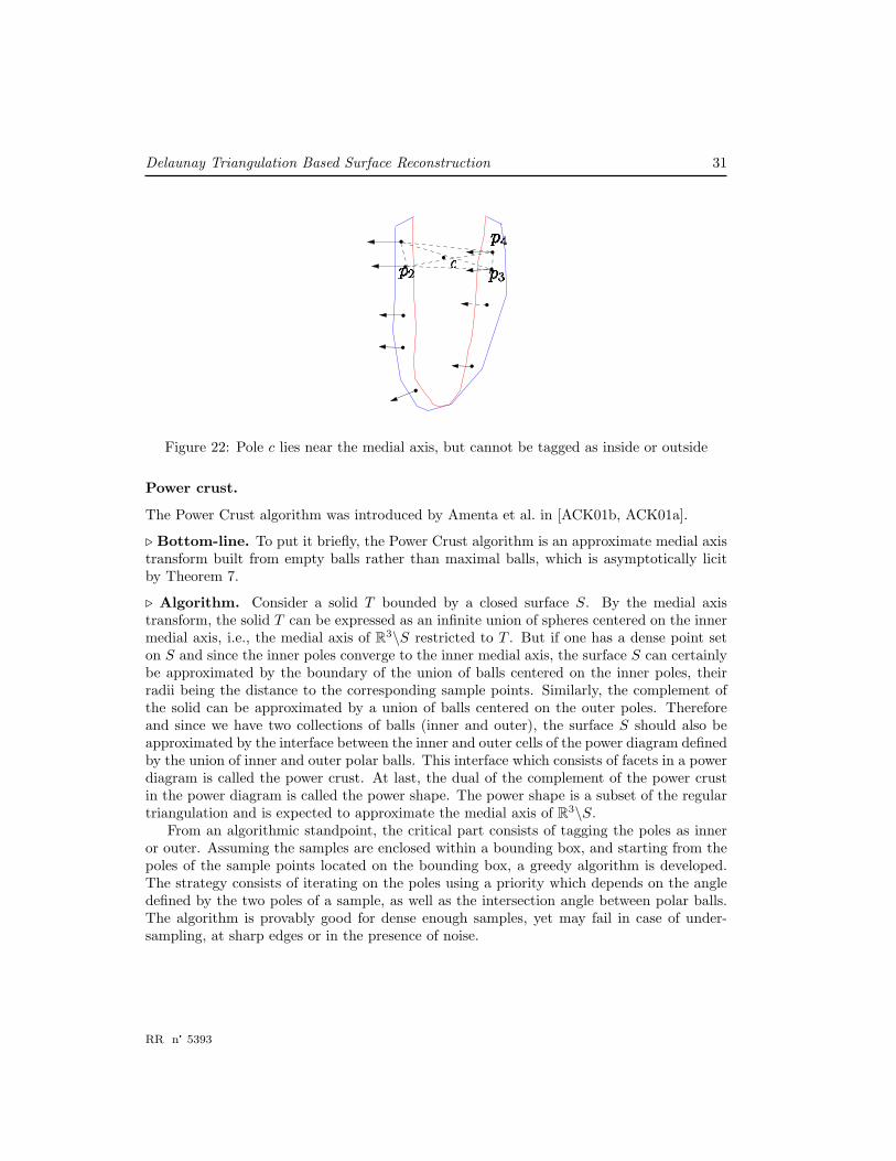
Figure 22: Pole c lies near the medial axis, but cannot be tagged as inside or outside

Power crust.

The Power Crust algorithm was introduced by Amenta et al. in [ACK01b, ACK01a].

. Bottom-line. To put it briefly, the Power Crust algorithm is an approximate medial axistransform built from empty balls rather than maximal balls, which is asymptotically licitby Theorem 7.

. Algorithm. Consider a solid T bounded by a closed surface S. By the medial axistransform, the solid T can be expressed as an infinite union of spheres centered on the innermedial axis, i.e., the medial axis of R3\S restricted to T . But if one has a dense point seton S and since the inner poles converge to the inner medial axis, the surface S can certainlybe approximated by the boundary of the union of balls centered on the inner poles, theirradii being the distance to the corresponding sample points. Similarly, the complement ofthe solid can be approximated by a union of balls centered on the outer poles. Thereforeand since we have two collections of balls (inner and outer), the surface S should also beapproximated by the interface between the inner and outer cells of the power diagram definedby the union of inner and outer polar balls. This interface which consists of facets in a powerdiagram is called the power crust. At last, the dual of the complement of the power crustin the power diagram is called the power shape. The power shape is a subset of the regulartriangulation and is expected to approximate the medial axis of R3\S.

From an algorithmic standpoint, the critical part consists of tagging the poles as inneror outer. Assuming the samples are enclosed within a bounding box, and starting from thepoles of the sample points located on the bounding box, a greedy algorithm is developed.The strategy consists of iterating on the poles using a priority which depends on the angledefined by the two poles of a sample, as well as the intersection angle between polar balls.The algorithm is provably good for dense enough samples, yet may fail in case of under-sampling, at sharp edges or in the presence of noise.

RR n° 5393

32 Cazals & Giesen

The surface reported is a watertight, i.e., a closed, piecewise linear surface consisting ofof power facets, yet possibly pinched at some points. All the sample points are interpolated,yet the result contains additional vertices.

. Complexity. Three data structures are used: the Delaunay triangulation of the originalsamples, the power diagram of the poles, and the the priority queue of the tagging algorithm.

. Guarantees. It is first proved that an inner and an outer ball intersect shallowly —seeFig. 21 for an illustration. This result was already present in [Att98] for the two-dimensionalcase.

Denoting UI (UO) the boundary of the union of inner (outer) balls, the following proper-ties are proved. The one-sided Hausdorff distance between UI and S is small, and so is thedistance between UO and S, as well as between the power-crust and S. The angle betweenthe normal at a point of UI or UO (where it is defined, i.e. on the interior of the sphericalcaps of UI and UO) and the normal at the nearest point on S is also small. This geometricproperty can be used to show that the projection of UI (or UO) to the nearest point on Sdefines a homeomorphism. Using a similar construction, it is also proved that the powercrust and the surface are homeomorphic. At last, the power shape is homotopy equivalentto the complement of the surface. Notice that providing more accurate guarantees on thepower shape is significantly more difficult due to the intricate structure of the medial axis,and also due to the fact that the power shape may contain flat tetrahedrons.

. Extensions. Noise and under-sampling are detected by analyzing the roundness ofVoronoi cells. Badly shaped cells and the corresponding poles are discarded. Discardingboth poles of a sample which fails the skinniness test allows to accommodate sharp edges asthe intersection of two facets of the power diagram. At last, large facets of the power crustwitnessed by an inner and an outer ball intersecting deeply can be removed, thus leaving asurface with boundary.

Natural Neighbors.

Natural neighbors were first used for reconstruction in [BC00, BC01a]. A reconstructionmethod based on these algorithms was integrated to CATIA version 5 in 2001.

. Bottom-line. It is well known by a theorem of Whitney that any smooth surface occursas the solution set f−1(0) for some smooth function f : R3 7→ R. The Natural Neighborsreconstruction method is based on the definition of such a function based on two ingredients:an estimate of the tangent plane based on the poles, and the natural coordinates definedwith respect to the Voronoi diagram of the samples.

. Algorithm. For the sake of clarity, first assume that each sample point is given withits normal vector ni. Denoting NNs(p) the natural neighbors of a point p and λi(p) thenatural coordinate of p with respect to pi, the method is based upon the following implicit

INRIA

Delaunay Triangulation Based Surface Reconstruction 33

function f : R3 7→ R:f(x) =

∑pi∈NNs(p)

λi 〈pix, ni〉.

The inner product 〈pix, ni〉 measures the signed distance from x to the tangent plane atpi, and the function f therefore averages the signed distances to the tangent planes ofthe natural neighbors of the point x. A direct consequence of the properties of naturalcoordinates is that the function f interpolates the point cloud, so that the reconstructedsurface S is naturally defined as f−1(0). It has been conjectured that S is a smooth surface,yet it remains to show that 0 is a regular value of f .

Since the natural coordinates have an involved expression, a triangulated approximationof S can be obtained as a subset of the Delaunay triangulation of the samples, namely asthe restricted Delaunay triangulation Df−1(0)(P ). This triangulation is easily computed asfollows. Denote by c1c2 the dual Voronoi edge of a triangle t. If f(c1)f(c2) < 0, then trianglet belongs to the restricted Delaunay. Such triangles are also called bipolar in this case.

If the normals are unknown, they can be estimated using the poles. Orienting thenormals is also possible using a greedy algorithm similar to the one used in [ACK01b] forthe Power-Crust algorithm.

. Complexity. Apart from the Delaunay triangulation, a priority queue is required to signthe poles and orient the normals if the normals are not provided.

. Guarantees. It can be shown that the Hausdorff distance between f−1(0) and S tendsto zero when the sampling density goes to infinity. There is no guarantee on the topologicalcoherence between the bipolar facets that make up the reconstruction since non manifoldedges may be encountered in case of boundaries, noise, or under-sampling. possible.

Topologically guided methods for the inside / outside labeling make use of the distancefunction induced by the sampling P . In section 2 we have already summarized some proper-ties of this function. In topological guided methods one wants to exploit the critical pointsof the distance function and their stable manifolds for reconstruction.

Wrap.

The Wrap algorithm was designed by Edelsbrunner [Ede04] already in 1995 and since thenmarketed by his company.

. Bottom-line. The Wrap algorithm is based on the concepts of flow and stable manifolds.But instead of building directly on the flow induced by the sample points a flow relation isdefined on the set of simplices of the Delaunay triangulation D(P ) of the sample points P .The critical points are defined exactly as for the distance function induced by P , i.e. as theintersection points of Delaunay- and their dual Voronoi objects. But their stable manifoldsare now approximated by subcomplexes of D(P ). The reconstruction produced by the Wrapalgorithm is the boundary of the union of stable manifolds of a subset of the maxima of theflow relation. As the boundary of a solid it is a surface.

RR n° 5393

34 Cazals & Giesen

. More details.The flow relation / ⊂ D × D on the set D of Delaunay simplices is defined as follows:

τ / ν/ σ if ν is a face of τ and σ and there exists a point x in the interior of ν such that there isan orbit φy that is passing from the interior of τ through x to σ. τ is called a predecessor andσ is called a successor of ν. The relation / is acyclic. A sink is a Delaunay tetrahedron thatcontains a maximum of the flow, i.e. its dual Voronoi vertex. The set of sinks is augmentedby an artificial sink at infinity. The flow relation can be used to define the ancestor andconservative ancestor sets of a set B of sinks. These sets consist of Delaunay simplices thatare that linked to a tetrahedron in B by a chain in the flow relation. The wrapping surfaceof the point set P is the boundary of the union of the ancestor sets of all finite sinks orequivalently it consists of the complement in the the Delaunay triangulation D(P ) of theconservative ancestor set of the sink at infinity. The wrapping surface is unique. It can becomputed by collapsing certain simplices. The collapse operation removes simplices that arethe unique proper coface of one of their faces. A collapse does not change the homotopytype of the complex since it can be seen as a deformation retraction which always retains thehomotopy type. Thus the complex bounded by the wrapping surface is homotopy equivalentto a point, i.e. the wrapping surface cannot be a torus for example. The latter disadvantageis bypassed by allowing a simplex removing operation that changes the homotopy type. Thedeletion is similar to the original definition of the wrapping surface. Instead of removing fromthe Delaunay triangulation D(P ) only the conservative ancestor set of the sink at infinity,the conservative ancestor sets of a set of sinks is removed. Consequently the wrappingsurface is now the boundary of the union of the ancestor sets of the remaining sinks. Thelatter union need not be homotopy equivalent to a point, i.e. the wrapping surface can betopologically more complicated.

. Guarantees. No reconstruction guarantees are given besides the fact that the wrappingsurface always is the boundary of a solid.

. Complexity. The running time of the Wrap algorithm is dominated by the time neededto compute the Delaunay triangulation D(P ), i.e., it is Θ(n2) where n is the size of P .

. Extensions. No extensions to the Wrap algorithm are known.

Flow complex.

The flow complex is very much related to the Wrap algorithm.

. Bottom-line. It was observed by Giesen and John [GJ02] that a reconstruction similarto the one obtained by the Wrap algorithm can be derived from the flow complex. The flowcomplex has a recursive structure, i.e., the stable manifolds of a critical point is boundedby stable manifolds of critical points of lower index. The reconstruction is the boundary ofthe union of all stable manifolds of the local maxima of the induced distance function. Thestable manifold of an index 2 saddle point can be either in the boundary of either one ortwo stable manifolds of local maxima. As in the Wrap algorithm one can recursively use

INRIA

Delaunay Triangulation Based Surface Reconstruction 35

stable manifolds of index 2 saddles which are in the boundary of only one stable manifold ofa local maximum to push the reconstruction further to interior of the complex. The pushingis guided by considering the difference in value of the height function at the local maximumand the index 2 saddle point.

. Algorithm. The flow complex is not a subcomplex of the Delaunay triangulation D(P )though D(P ) can be used to compute the flow complex. This computation is quite involvedand makes use of the recursive structure of the stable manifolds. Here we want to refer thereader to [GJ03] for a detailed description.

. Guarantees. No reconstruction guarantees are given besides the fact that the wrappingsurface always is the boundary of a solid.

. Complexity. The combinatorial and algorithmic complexities of the flow complex are notknown yet. The reconstruction has roughly three times as many triangles as other Delaunaybased reconstruction algorithms.

. Extensions. No extensions are known.

Convection algorithm.

The convection algorithm was designed by Chaine [Cha03].

. Bottom-line. The Convection algorithm is the geometric implementation of the convec-tion model introduced by Zhao, Osher and Fedkiw []. In this model it is proposed to use asurface S as the reconstruction of S from P that minimizes the following energy functional

E(S′) =(∫

x∈S′hp(x) dx

)1/p

, 1 ≤ p ≤ ∞,

where the integral is taken over the closed surface S′ and h is the distance function inducedby the sampling P . Zhao et al. propose an evolution equation to construct the surface thatminimizes the energy functional by deforming a good initial enclosing approximation of thesurface. The evolution follows the gradient descent of the energy functional. Every point xof the surface S′ evolves towards the interior of the surface along the normal direction n ofS′ at x with speed proportional to −∇h(x) · n + t(x), where t(x) is the surface tension ofS′ at x. To compute an initial approximation of S Zhao et al. change the evolution in thesense the the velocity field at each point x ∈ S′ is replaced by −∇h(x). Chaine proves thefollowing theorem for this approximation approach.

Theorem 9 Given a closed surface S′ enclosing the point set P then S′ evolves under theconvection −∇h(x) to a set of closed, piecewise linear pseudo-surfaces. All the facets of thesepseudo-surfaces are Delaunay triangles that have the oriented Gabriel property where thetriangles are oriented such that their normal points to the inside of the bounded componentenclosed by the pseudo-surface.

RR n° 5393

36 Cazals & Giesen

A pseudo surface can be pinched together along some of its subsets. To define the orientedGabriel property let t be a Delaunay triangle with oriented normal n. Let s be the half-sphereof the minimum enclosing sphere of t that is contained in half space bounded by the affinehull of t and pointed into by n. The triangle t has the oriented Gabriel property if the halfsphere s does not contain any point from P in its interior. Chaine observed that Theorem 9can be turned into an algorithm based on the Delaunay triangulation D(P ) of the samplepoints P . In this algorithm the evolving pseudo surface is initialized with the boundaryof the convex hull of P and all the triangles on this boundary are oriented to point insidethe convex hull. The pseudo surface evolves by pushing into Delaunay tetrahedrons. Thepushing operations are determined by the vector field −∇h(x) and topological constraints.

. Algorithm. The algorithm basically works as follows: As long as there is a facet f in theevolving, oriented, pseudo surface S′ that does not have the oriented Gabriel property do thefollowing. If the facet f with the inverse orientation also belongs to S′ then remove f fromS′. Otherwise replace f by the three Delaunay facets incident to the Delaunay tetrahedronwhich is incident to f and on the positive side of f with respect to the orientation of f .Orient the three new facets in S′ properly such that their normals point into the interior ofthe evolving pseudo surface.

. Guarantees. No reconstruction guarantees are given.

. Complexity. The running time of the Convection algorithm is dominated by the timeneeded to compute the Delaunay triangulation D(P ), i.e., it is Θ(n2) where n is the size ofP .

. Extensions. One modification of the Convection algorithm is to keep an oriented facet fin S′ if the same facet with the inverse orientation is also in S′. In doing so the convectionalgorithm can also reconstruct surfaces with boundaries.

Sometimes the Convection algorithm stops too early, i.e., one would like to push theevolving surface even further. A heuristic to do so is provided.. Comments. The Convection algorithm is dual to the Wrap algorithm (and the Flowcomplex) in the sense that the direction of “flow” is reversed. The Wrap algorithm retains thepart of the Delaunay triangulation that does not “flow” to infinity whereas the Convectionalgorithm lets the convex hull of P “flow” towards the shape.

3.4 Empty balls methods

A triangle reported in a reconstructed surface should be local in some sense. One way tospecify locality is to use the empty ball property.

Ball pivoting algorithm

Bernardini et al. designed the ball pivoting algorithm to compute a surface subset of anα-shape of a sampling P in linear time and space [].

INRIA

Delaunay Triangulation Based Surface Reconstruction 37

. Bottom-line and algorithm. Like in the definition of α-shapes a triangle pqr withvertices p, q, r ∈ P forms a triangle in the reconstruction if there is a ball of radius α thatcontains p, q and r in its boundary and no point from P in its interior. Starting with an α-exposed seed triangle the ball pivoting algorithm pivots around an edge of the seed triangle,i.e., it revolves around an edge while keeping the edge’s endpoints on its boundary, untilit touches another point from P , forming another triangle. This process continues until allreachable edges have been processed. Then the process continues with a new seed triangleuntil all points in P have been considered.

. Guarantees. No guarantees are given.

. Complexity. Time and space complexity of the ball pivoting algorithm are linear, i.e., itis asymptotically faster than computing the Delaunay triangulation D(P ) of P .

. Extensions. To accommodate non-uniform sampling the pivoting process can be repeatedwith a larger value for α.

Regular interpolant

The regular interpolant was introduced in [PB01] by Petitjean and Boyer. Their workstresses the importance of Gabriel triangles for surface reconstruction, an observation alsoraised in [AS00].

. Bottom-line. The framework of ε-samples might not be the definitive set-up for solvingpractical problems. To bypass this difficulty, Petitjean and Boyer address the issue of findingan interpolant encoding the properties of the sampling P rather than those of an hypotheticalsmooth surface S. To see how, we first introduce the relevant notions.

An interpolant O in R3 is a 2-simplicial complex having P as vertex set. The interpolantis closed if each simplex bounds two distinct connected components of the ambient space.Notice that this definition does not subsume any manifoldness property.

Given a sample point p ∈ P , its granularity g(p) is defined as the radius of the largestball circumscribing a triangle incident to p.

Now, given an interpolant, its associated discrete medial axis is the Voronoi diagramfrom which one removes the Voronoi cells dual to simplices of the interpolant. Notice thatthe process leaves Voronoi cells of dimensions from two to zero, and in particular all theVoronoi vertices.

The discrete feature size or local thickness t(p) at a sample point p is its least distance tothe discrete medial axis with the convention t(p) = 0 if p is on the boundary of a connectedcomponent of R3\O which does not contain any piece of the discrete medial axis.

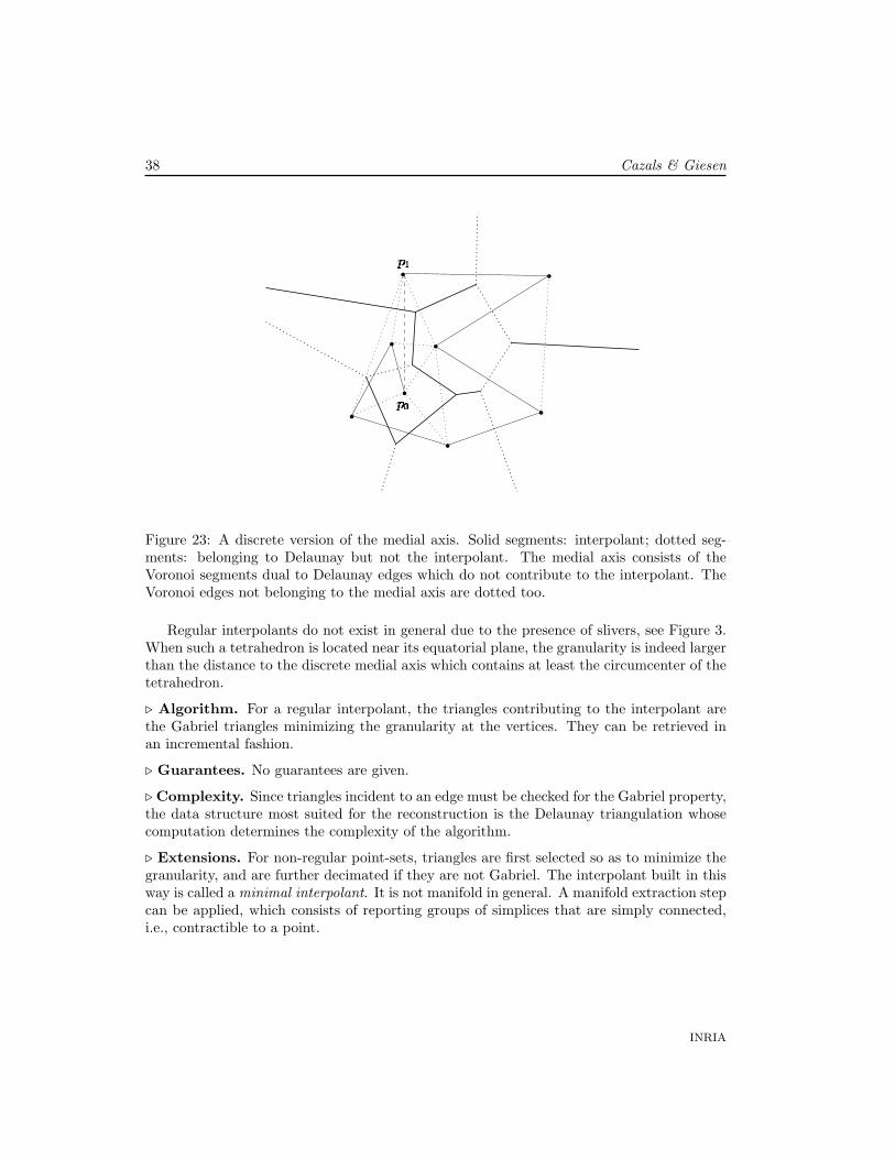
Equipped with these notions, an interpolant is called regular is g(p) < t(p) for all samplepoints p. Getting back to the point cloud, P is said to be regular if it admits at least oneregular interpolant. These notions are depicted in Figure 23.

RR n° 5393

38 Cazals & Giesen

� �

� �

Figure 23: A discrete version of the medial axis. Solid segments: interpolant; dotted seg-ments: belonging to Delaunay but not the interpolant. The medial axis consists of theVoronoi segments dual to Delaunay edges which do not contribute to the interpolant. TheVoronoi edges not belonging to the medial axis are dotted too.

Regular interpolants do not exist in general due to the presence of slivers, see Figure 3.When such a tetrahedron is located near its equatorial plane, the granularity is indeed largerthan the distance to the discrete medial axis which contains at least the circumcenter of thetetrahedron.

. Algorithm. For a regular interpolant, the triangles contributing to the interpolant arethe Gabriel triangles minimizing the granularity at the vertices. They can be retrieved inan incremental fashion.

. Guarantees. No guarantees are given.

. Complexity. Since triangles incident to an edge must be checked for the Gabriel property,the data structure most suited for the reconstruction is the Delaunay triangulation whosecomputation determines the complexity of the algorithm.

. Extensions. For non-regular point-sets, triangles are first selected so as to minimize thegranularity, and are further decimated if they are not Gabriel. The interpolant built in thisway is called a minimal interpolant. It is not manifold in general. A manifold extraction stepcan be applied, which consists of reporting groups of simplices that are simply connected,i.e., contractible to a point.

INRIA

Delaunay Triangulation Based Surface Reconstruction 39

4 Evaluating surface reconstruction algorithms

Evaluating surface reconstruction algorithms is a difficult task. A prominent feature of someof the algorithms presented in this chapter is that these algorithms come with theoreticalguarantees under certain conditions. But if these conditions are not met, their behavioris not specified. Thus it is an interesting question how reconstruction algorithms performon “real data”. In order to assess the performance of different algorithms on real data twosurface reconstruction challenges have been organized. One challenge was organized withinthe Effective Computational Geometry project, a project funded by the European Union.The other challenge was organized within a DIMACS Workshop. For both challenges severaldata sets featuring the following difficulties were selected: undersampling, sharp features,thin parts, boundaries, high genus, noise.

The reader is referred to www-sop.inria.fr/prisme/manifestations/ECG02/SurfReconsTestbed.html

and www.cse.ohio-state.edu/dimacs-sr-challenge where the data sets usded in the chal-lenges are available.

References

[AB99] Nina Amenta and Marshall Bern. Surface reconstruction by Voronoi filtering.Discrete Comput. Geom., 22(4):481–504, 1999.

[ABCO+01] M. Alexa, J. Behr, D. Cohen-Or, S. Fleishman, D. Levin, and C. Silva. Pointset surfaces. In IEEE, editor, Visualization, 2001.

[ABE98] Nina Amenta, Marshall Bern, and David Eppstein. The crust and the β-skeleton: Combinatorial curve reconstruction. Graphical Models and ImageProcessing, 60:125–135, 1998.

[ABL03] D. Attali, J.-D. Boissonnat, and A. Lieutier. Complexity of the delaunay tri-angulation of points on surfaces the smooth case. In ACM SoCG, San Diego,2003.

[ACDL00] N. Amenta, S. Choi, T. K. Dey, and N. Leekha. A simple algorithm for home-omorphic surface reconstruction. In Proc. 16th Annu. ACM Sympos. Comput.Geom., pages 213–222, 2000.

[ACK01a] N. Amenta, S. Choi, and R. Kolluri. The power crust. In ACM Solid Modeling,2001.

[ACK01b] N. Amenta, S. Choi, and R. K. Kolluri. The power crust, unions of balls, andthe medial axis transform. Comput. Geom. Theory Appl., 19:127–153, 2001.

[AS00] M. Attene and M. Spagnuolo. Automatic surface reconstruction from pointsets in space. In Eurographics, 2000.

RR n° 5393

40 Cazals & Giesen

[Att98] D. Attali. r-regular shape reconstruction from unorganized points. Comput.Geom. Theory Appl., 10:239–247, 1998.

[Aur88] F. Aurenhammer. Linear combinations from power domains. Geom. Dedicata,28:45–52, 1988.

[BC00] Jean-Daniel Boissonnat and Frederic Cazals. Smooth surface reconstructionvia natural neighbour interpolation of distance functions. In Proc. 16th Annu.ACM Sympos. Comput. Geom., pages 223–232, 2000.

[BC01a] Jean-Daniel Boissonnat and Frederic Cazals. Coarse-to-fine surface simplifi-cation with geometric guarantees. In A. Chalmers and T.-M. Rhyne, editors,Eurographics’01, Manchester, 2001. Blackwell.

[BC01b] Jean-Daniel Boissonnat and Frederic Cazals. Natural coordinates of points ona surface. Comput. Geom. Theory Appl., 19:155–173, 2001.

[Boi84] Jean-Daniel Boissonnat. Geometric structures for three-dimensional shape rep-resentation. ACM Trans. Graph., 3(4):266–286, 1984.

[Bro97] J. L. Brown. Systems of coordinates associated with points scattered in theplane. Comput. Aided Design, 14:547–559, 1997.

[CBC+01] J. Carr, R. Beatson, J. Cherrie, T. Mitchell, T. Fright, B. McCallum, andT. Evans. Reconstruction and representation of 3d objects with radial basisfunctions. In Siggraph. ACM, 2001.

[CDE+99] Siu-Wing Cheng, Tamal K. Dey, Herbert Edelsbrunner, Michael A. Facello,and Shang-Hua Teng. Sliver exudation. In Proc. 15th Annu. ACM Sympos.Comput. Geom., pages 1–13, 1999.

[cga] The cgal library.

[Cha03] R. Chaine. A convection geometric-based approach to surface reconstruction.In Symp. Geometry Processing, 2003.

[CSD04] D. Cohen-Steiner and F. Da. A greedy delaunay based surface reconstructionalgorithm. The Visual Computer, 2004. To appear.

[DG03] T. K. Dey and S. Goswami. Tight cocone: A water-tight surface reconstruc-tor. Journal of Computing and Information Science in Engineering, 3:302–307,2003.

[DG04] T.K. Dey and S. Goswami. Provable surface reconstruction from noisy samples.In ACM SoCG, 2004.

INRIA

Delaunay Triangulation Based Surface Reconstruction 41

[Ede04] H. Edelsbrunner. Surface reconstruction by wrapping finite point sets in space.In B. Aronov, S. Basu, J. Pach, and M. Sharir, editors, Ricky Pollack and EliGoodman Festschrift, pages 379–404. Springer-Verlag, 2004(?).

[EM90] H. Edelsbrunner and E. P. Mucke. Simulation of simplicity: A technique to copewith degenerate cases in geometric algorithms. ACM Trans. Graph., 9(1):66–104, 1990.

[ES97] H. Edelsbrunner and N. R. Shah. Triangulating topological spaces. Int. J. onComp. Geom., 7:365–378, 1997.

[GJ02] J. Giesen and M. John. Surface reconstruction based on a dynamical system.In Proceedings of the 23rd Annual Conference of the European Association forComputer Graphics (Eurographics), Computer Graphics Forum 21, pages 363–371, 2002.

[GJ03] J. Giesen and M. John. The flow complex: A data structure for geometricmodeling. In ACM SODA, 2003.

[GK00] P. Giblin and B. Kimia. A formal classification of 3d medial axis points andtheir local geometry. In Computer Vision and Pattern Recognition, HiltonHead, South Carolina, USA, 2000.

[GKS00] M. Gopi, S. Krishnan, and C.T. Silva. Surface reconstruction based on lowerdimensional localized delaunay triangulation. In Eurographics, 2000.

[HOF01] H.K.Zhao, S. Osher, and R. Fedkiw. Fast surface reconstruction using the levelset method. In IEEE, editor, IWorkshop on Variational and Level Set Methods,2001.

[HS02] H. Hiyoshi and K. Sugihara. Improving continuity of voronoi-based interpola-tion over delaunay spheres. Comput. Geom., 22(1-3), 2002.

[MT02] J-M. Morvan and B. Thibert. Smooth surface and triangular mesh : Compar-ison of the area, the normals and the unfolding. In ACM Symposium on SolidModeling and Applications, 2002.

[PB01] S. Petitjean and E. Boyer. Regular and non-regular point sets: Properties andreconstruction. Comput. Geom. Theory Appl., 19:101–126, 2001.

[Sib81] R. Sibson. A brief description of natural neighbour interpolation. In Vic Bar-net, editor, Interpreting Multivariate Data, pages 21–36. John Wiley & Sons,Chichester, 1981.

[Yom81] Y. Yomdin. On the general structure of a generic central set. Compositio Math,43, 1981.

RR n° 5393

42 Cazals & Giesen

Contents

1 Introduction 31.1 Surface reconstruction . . . . . . . . . . . . . . . . . . . . . . . . . . . . . . . 31.2 Applications . . . . . . . . . . . . . . . . . . . . . . . . . . . . . . . . . . . . . 31.3 Reconstruction using the Delaunay triangulation . . . . . . . . . . . . . . . . 31.4 A classification of Delaunay based surface reconstruction methods . . . . . . 51.5 Organization of the chapter . . . . . . . . . . . . . . . . . . . . . . . . . . . . 5

2 Pre-requisites 62.1 Delaunay triangulations, Voronoi diagrams and related concepts . . . . . . . 62.2 Medial axis and derived concepts . . . . . . . . . . . . . . . . . . . . . . . . . 152.3 Topological and geometric equivalences . . . . . . . . . . . . . . . . . . . . . . 20

3 Overview of the algorithms 233.1 Tangent plane based methods . . . . . . . . . . . . . . . . . . . . . . . . . . . 233.2 Restricted Delaunay based methods . . . . . . . . . . . . . . . . . . . . . . . 263.3 Inside / outside labeling . . . . . . . . . . . . . . . . . . . . . . . . . . . . . . 303.4 Empty balls methods . . . . . . . . . . . . . . . . . . . . . . . . . . . . . . . . 36

4 Evaluating surface reconstruction algorithms 39

INRIA

Unite de recherche INRIA Sophia Antipolis2004, route des Lucioles - BP 93 - 06902 Sophia Antipolis Cedex (France)

Unite de recherche INRIA Futurs : Parc Club Orsay Universite - ZAC des Vignes4, rue Jacques Monod - 91893 ORSAY Cedex (France)

Unite de recherche INRIA Lorraine : LORIA, Technopole de Nancy-Brabois - Campus scientifique615, rue du Jardin Botanique - BP 101 - 54602 Villers-les-Nancy Cedex (France)

Unite de recherche INRIA Rennes : IRISA, Campus universitaire de Beaulieu - 35042 Rennes Cedex (France)Unite de recherche INRIA Rhone-Alpes : 655, avenue de l’Europe - 38334 Montbonnot Saint-Ismier (France)

Unite de recherche INRIA Rocquencourt : Domaine de Voluceau - Rocquencourt - BP 105 - 78153 Le Chesnay Cedex (France)

EditeurINRIA - Domaine de Voluceau - Rocquencourt, BP 105 - 78153 Le Chesnay Cedex (France)

http://www.inria.fr

ISSN 0249-6399