Degenerated Four Nodes Shell Element with Drilling …iosrjen.org/Papers/vol3_issue8 (part-3)/B03831020.pdf · combining the constant strain triangle (CST) element for membrane stiffness

IOSR Journal of Engineering (IOSRJEN)

e-ISSN: 2250-3021, p-ISSN: 2278-8719 Vol. 3, Issue 8 (August. 2013), ||V3 || PP 10-20

www.iosrjen.org 10 | P a g e

Degenerated Four Nodes Shell Element with Drilling Degree of

Freedom

Fathelrahman. M. Adam1, Abdelrahman. E. Mohamed

2, A. E. Hassaballa

3

1Dept. of Civil Engineering, Jazan University, Kingdom of Saudi Arabia 2Dept. of Civil Engineering, Sudan University of Science and Technology, Sudan.

3Dept. of Civil Engineering, Jazan University, Kingdom of Saudi Arabia

Abstract: - A four node degenerated shell element with drilling degree of freedom is presented in this paper.

The problem of zero stiffness that appears with using the drilling degree of freedom and causes singularity in the

structure stiffness matrix is solved by employing, one of the recommended remedies. That is, adding a fictitious

rotational stiffness using a penalty parameter (torsional constant) to control the solution to insure good element

performance. Examples are presented including comparisons of torsional constant with the maximum

displacements by using different mesh sizes, which results on selecting a value equal to one for the torsional

constant is suitable value used to insure rapid convergence to true solution.

Keywords: - Degenerated shell, drilling degree of freedom, fictitious rotational stiffness, Tensional constant.

I. INTRODUCTION Drilling or in-plane rotational, degrees of freedom have been introduced with various meanings and

purposes to model displacements in planar finite elements. The need for membrane elements with drilling

degrees of freedom arises in many practical engineering problems such as in-filled frames and folded plates.

This special practice is frequently used in the analysis of thin shells by the finite element method. It is, basically,

to allow correct modeling of the junction between angles of shell elements and to simplify the modeling of

connections between plates, shells and beams, as well as the treatment of the junctions of the shells and box

girders. Several work was initiated since 1964 for developing membrane finite elements with drilling degrees of

freedom (Djermane (2006) [1] and Allman (1988) [2]). The assembly of the stiffness matrices of membrane and

bending components at each node will result in a zero value on the diagonal corresponding to the drilling degree

of freedom since this is not considered in the membrane or bending element as stated by Zeinkiewicz and Taylor (2000) [3], Alvin et al. (1992) [4], Felippa and Militello (1992) [5] and Felippa and Scot (1992) [6]. This zero

stiffness for the drilling degree of freedom causes singularity in the structure stiffness matrix when all the

elements are coplanar and there is no coupling between the membrane and bending stiffness of the element.

Several methods have been suggested by various authors for removing the singularity in the stiffness

matrix based on variational principles such as those formulated by Gruttmann et al. (1992) [7]. These elements

are stable and perform very well in non-linear problems. Knight (1997) [8] suggested that a very small value be

specified for the stiffness of the drilling degrees of freedom so that the contribution to the strain energy equation

from this term will be zero. Bathe and Ho (1981) [9] approximated the stiffness for drilling degrees of freedom

by using a small approximate value. Batoz and Dhatt (1972) [10] presented the formulation of a triangular shell

element named KLI element with 15 degrees of freedom and a quadrilateral shell element named KQT element

with 20 degrees of freedom using the discrete Kirchoff formulation of plate bending element. The KQT element was developed by combining four triangular elements with the mid-nodes on the sides. The KQT element was

found to be more effective among the two. Bathe and Ho (1981) [9] developed a flat shell triangular element by

combining the constant strain triangle (CST) element for membrane stiffness and the plate bending element

using the Mindlin theory of plates for the bending stiffness. They introduced a fictitious stiffness for the drilling

degrees of freedom in the development of the element stiffness matrix for the triangular flat shell element. This

element was found to be very effective for the analysis of shell structures. McNeal (1978) [11] developed the

quadrilateral shell element QUAD4, by considering two in-plane displacements that represent membrane

properties and one out-of-plane displacement and two rotations, which represent the bending properties. He

included modifications in terms of a reduced order integration scheme for shear terms. He also included

curvature and transverse shear flexibility to deal with the deficiency in the bending strain energy. The first

successful triangles with drilling freedoms were presented by Allman in (1984) [12] and Bergan and Felippa in

(1985) [13]. A degenerated shell element with drilling degrees of freedom was developed recently by Djermane et al. (2006) [1] for application in linear and nonlinear analysis of thin shell structures for isotropic or

anisotropic materials with using the assumed natural strains technique to alleviate locking phenomenon. The

Degenerated Four Nodes Shell Element with Drilling Degree of Freedom


same authors extended the formulation by using the same techniques to study the dynamic responses of thick

and thin nonlinear shells (Djermane et al. (2007) [14]).

Thus, the simplest method adopted to remove the rotational singularity is to add a fictitious rotational stiffness. However, Yang (2000) [15] suggested that, although the method solves the problem of singularity it

creates a convergence problem that sometimes leads to poor results. A number of alternatives have been

proposed by Adam and Mohamed (2013) [16] for avoiding the presence of this singular behavior. One of the

remedies is to utilize the original penalty approach of Kanok–Kanukulchai (1979) [17], by introducing a

constraint equation which “links” the drilling rotations in the fiber coordinate system to the in-plane twisting

mode of the mid-surface. An additional energy functional can be then defined in the standard manner, to allow

the application of the penalty method giving the preceding definition of the drilling degree of freedom with the

fictitious torsional coefficient serving as a penalty parameter. Numerical experiments showed that the element

performance is very sensitive to penalty parameter value as stated by Guttal and Fish (1999) [18].

In this paper a bilinear degenerated four nodes shell elements is developed. Five numerical examples

are used to examine the element performance with respect to sensitivity to the value of penalty parameter and to evaluate the suitable value.

II. DEGENERATED FOUR NODES SHELL ELEMENT FORMULATION This element was presented by Kanock-Nukulchai (1979) [17] under the following assumptions:

1. Normal to the mid-surface remains straight after deformation.

2. Stresses normal to the mid-surface are zero.

2.1 Geometric shape:

A four nodes element is obtained by degenerating the eight nodes solid element as shown in Fig. (2.1).

Fig. (2.1): Four nodes shell element degenerated from eight nodes solid element

Fig. (2.2): Four nodes shell element

The midsurface shown in Fig. (2.2) is defined by natural coordinates (r, s, t). The displacements u, v

and w are the displacements in global Cartesian coordinates x, y and z respectively. θx, θy, and θz are rotations about the x, y and z respectively. The rotations αx, αy and αz are about local coordinates x', y', and z' respectively.

r

s

t

x'

y' z'

z(w) y(v)

θy

θz

αy

αx

αz

θx

1

2

3

4

x(u)

1

5 2

3

4 6

7

8 3

4

1

2



The shape functions to describe the midsurface in terms of natural coordinates are:

Ni (r,s) = ¼(1 + ri r) (1 + si s) (2.1)

The thickness at each node hi is computed in the direction normal to the midsurface.

Fig.(2.3): Node director

From Fig.(2.3) vector V3i is called node director and defined by:

V3i

bottomitopi

bottomitopi

bottomitopi

zz

yy

xx

(2.2)

The coordinates of any point in the element can be derived from the 8-nodes solid element to 4-nodes element

as:

bottomi

i

i

i ii

topi

i

i

i

z

y

x

Nt

z

y

x

Nt

z

y

x

4

1

4

1

)1(2

1)1(

2

1 (2.3)

Since )1(2

1t is the part of shape function in 8-nodes solid element in direction of the thickness.

and xi, yi and zi are the global coordinates of the midpoint i

2.2 Displacement field:

The displacement variation in the element can be expressed as:

4

1 *

*

*

i

i

i

i

i

i

i

i

w

v

u

w

v

u

N

w

v

u

(2.4)

Where ui, vi and wi are the displacements at mid point i along global direction, and ***, iii wandvu are

the relative nodal displacements along global direction produced by rotation of the normal at node i and can be expressed in terms of rotations θxi, θyi, and θzi at each node i about global axes. Using the assumption that

straight normal to the midsurface remains straight after deformation, the displacements produced by the

rotations αxi , αyi can be found as shown in Fig.(2.4) as:

02'

'

'

xi

yi

i

i

i

i

ht

w

v

u

(2.5)

where ''' , iii wandvu are the displacements components along local axes at node i. To transform these

displacements to global axes, transformation matrix T (Eqn.(2.6)) can be used.

Fig. (2.4): Rotation of normal due to αx and αy

αy

h/2

h/2αy

h/2αyt

t h/2

x'

z'

αx

h/2αx

h/2αxt

y'

z'

Bottom

node

Top node

i

V3i



T =

321

321

321

nnn

mmm

lll

(2.6)

where l1, m1 and n1 (the direction cosines) are components of unit vector v1, and l2, m2 and n2 are components of unit vector v2 , and l3, m3 and n3 are components of unit vector v3, then

*

*

*

i

i

i

w

v

u

Ti

0

'

'

i

i

v

u

=

xi

yi

ii

ii

ii

i

nn

mm

ll

ht

21

21

21

2 (2.7)

αxi and αyi are expressed in terms of global rotations θxi, θyi, and θzi by using transformation matrix Ti as:

xi

yi

=

zi

yi

xi

iii

iii

nml

nml

111

222 (2.8)

Substituting Eqn.(2.8) in Eqn.(2.7) gives:

*

*

*

i

i

i

w

v

u

zi

yi

xi

ii

ii

ii

i

lm

ln

mn

ht

0

0

0

233

33

33

(2.9)

And Substituting this in Eqn.(2.4), gives:

4

1

33

33

33

2i

yiixii

xiizii

ziiyii

i

i

i

i

i

lm

nl

mn

ht

w

v

u

N

w

v

u

(2.10)

2.3 Strain-displacement relation: By assuming that the strain normal to midsurface εz' = 0, the strains components along the local axes are given

by:

''

''

''

'

'

zy

zx

yx

y

x

=

'

'

'

'

'

'

'

'

'

'

'

'

'

'

'

'

y

w

z

v

x

w

z

u

x

v

y

u

y

v

x

u

(2.11)

By splitting Eqn. (2.11) to two components, membrane component and shear component it can be rewritten as:

''

'

'

yx

y

x

= (Bm1 + t Bm2) u (2.12)

''

''

xy

zx

= (Bs1 + t Bs2) u (2.13)

The matrices Bm1, Bm2, Bs1 and Bs2 can be derived by using Eqn. (2.14).

',','

',','

zyx

wvu

= Tu

zyx

wvu

,,

,,

(2.14)



Where Tu is the transformation matrix needed to transform the derivatives of Eqn. (2.14).

2.4 Stress-strain relation: The stress-strain relation can be stated after imposing σz' = 0 as:

''

''

''

'

'

zy

zx

yx

y

x

=

2

)1(0000

02

)1(000

002

)1(00

0001

0001

1

'2

E

''

''

''

'

'

zy

zx

yx

y

x

(2.15)

where = 5/6 is a factor that accounts for the thickness-direction variation of transverse shear strain, E' is the

modulus of elasticity and is Poisson's ratio. The constitutive matrix in Eqn. (2.15) is split into Cm and Cs as follows:

Cm =

2

100

01

01

1 2

E, Cs =

10

01

)1(2

E (2.16)

2.5 Element stiffness matrix:

The stiffness matrix can be split into two matrices, membrane and bending effects and transverse shear effects and can be written as:

Km =

1

1-

1

1

1

1

(Bm1 + t Bm2)T Cm (Bm1 + t Bm2) det J dr ds dt (2.17)a

Ks =

1

1-

1

1

1

1

(Bs1 + t Bs2)T Cs (Bs1 + t Bs2) det J dr ds dt (2.17)b

Integrating Eqn. (2.17)a and Eqn. (2.17)b directly across the thickness with respect to t, gives:

Km =

1

1-

1

1

2211 )(3

2)(2 mm

Tmmm

Tm BCBBCB det J dr ds (2.18)a

Ks =

1

1-

1

1

2211 )(3

2)(2 ss

Tsss

Ts BCBBCB det J dr ds (2.18)b

2.6 Torsional stiffness matrix

In a degenerated shell, the rotation of the normal and the mid-surface displacement field are independent. The

idea then is to derive an additional constraint between the torsional rotation of the normal, αz, and the rotation of

the mid-surface,

'

'

'

'

2

1

y

u

x

v [17].

Fig. (2.5) Torsional rotation of the normal and midsurface

The derivation of the torsional rotation of the normal from that of the midsurface is assumed to have governing

strain energy [4] and [17] as:

αz

'

'

'

'

2

1

y

u

x

v



Ut = αt G dAy

u

x

v

sr

A z

2

)0,,('

'

'

'

2

1

= uT Kt u (2.19)

where αt is the torsional constant and it is problem dependent, G is the shear modulus, and '

'

x

v

and

'

'

y

u

can be

calculated from Eqn. (2.14).

The matrix B3 can be written after extracting the vector of nodal displacements u from the relation

'

'

'

'

2

1

y

u

x

vz , then the torsional stiffness matrix is given by:

Kt = αt G

1

1

1

1

33 BBT dA (2.20)

αt is a penalty parameter and must be determined to insure good convergence.

III. NUMERICAL EXAMPLES To examine the effects of torsional constant (αt ) in the solution, a program was developed for the

degenerated shell element formulation and five numerical examples with different geometric shapes and

different support conditions were employed using different values for αt ranging from 1E-5 to 1E+5, with

different mesh sizes and the resulting maximum displacements were recorded.

By plotting the displacements versus αt using these meshes for the five Examples, the effect of αt value,

the rate of convergence and the suitable mesh size that gives a displacement value close to the exact value are

determined.

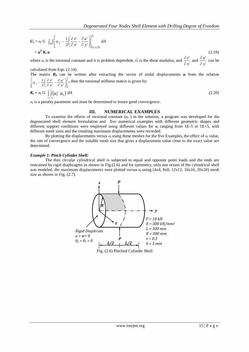
Example 1: Pinch Cylinder Shell:

The thin circular cylindrical shell is subjected to equal and opposite point loads and the ends are

restrained by rigid diaphragms as shown in Fig.(2.6) and for symmetry, only one octant of the cylindrical shell

was modeled. the maximum displacements were plotted versus αt using (4x4, 8x8, 12x12, 16x16, 20x20) mesh size as shown in Fig. (2.7).

Fig. (2.6) Pinched Cylinder Shell

x

R

L/2 L/2

y

P

P z

P = 10 kN E = 300 kN/mm2 L = 300 mm R = 300 mm ν = 0.3 h = 3 mm

Rigid Diaphram u = w= 0 θy = θz = 0



Fig. (2.7) Tensional Constant versus Maximum Displacement with Different Mesh Size for Example 1

Example 2: Scordelis-Lo roof:

The shell is supported on rigid diaphragms at the curved edge and free at straight edges and is loaded

by its own weight and for symmetry, only one quarter of the roof shown in Fig. (2.8) was analyzed using (4x4,

8x8, 12x12, 16x16 and 20x20) meshes. The maximum displacements were plotted versus αt for the different

mesh sizes as shown in Fig. (2.9).

Fig. (2.8) Scordelis-Lo roof


Example 3: Short Cantilever Beam under End Shear Load:

A shear-loaded cantilever beam, as shown in Figure (2.10) was idealized using 4x2, 8x2, 16x4 and 32x8 element

meshes. The maximum displacements were plotted versus αt for the different mesh sizes as shown in Fig. (2.11).

40° R = 25 ft

25 ft

x

Rigid Diaphram

Free Edge

Self Weight = 90 lb/ft2 E = 4.32 x108lb/ft2 ν = 0.0 h = 0.25 ft

z

y



Fig. (2.10) Short Cantilever Beam


Example 4: Folded plate simply supported on two opposite sides

The folded plate is simply supported on two opposite sides and is loaded by uniformly distributed load

along the ridge. For symmetry, only one quarter of the shell was analyzed using (4x4, 8x8, 12x12, 16x16 and 20x20) meshes. The maximum displacements were plotted versus αt for the different mesh sizes as shown in Fig.

(2.13).

Fig. (2.12) Folded plate simply supported on two opposite sides

x

h

L b

z

y

w

L = 50 in, b = 50 in, h = 25 in w = 4000 lb/in E = 1.0 x107 lb/in2 ν = 0.3 t = 0.1 in

h = 12 in

Total Shear Load = 40,000 lb

x

z

L = 48 in

Width = 1 in

E = 30000 lb/in2 ν = 0.25




Example 5: Clamped Hyperbolic Paraboloid Shell

The shell shown in Fig. (2.14) is the hyperbolic paraboloid shell and is clamped on four edges and

subjected to a uniform normal pressure. For symmetry, only one quarter of the shell was modeled using (4x4,

8x8, 12x12, 16x16 and 20x20) meshes. The maximum displacements were plotted versus αt for the different

mesh sizes as shown in Fig. (2.15).


x

50 in

50 in

10 in

z

Normal Pressure = 0.01 lb/in2 E = 28,500lb/in2 ν = 0.4 t = 0.8 in

y



IV. DISCUSSION As can be seen from the plottings of the torsional constants versus maximum displacements using

different mesh sizes for the five examples (figures 2.7, 2.9, 2.11, 2.13 and 2.15), using a small value, from 1 to

1E-5, for the torsional constant gives a high and constant value of maximum displacement which leads to rapid

convergence. The displacement variation lines for the different meshes tend to be straight and parallel to the line

of exact displacements starting from αt equal to one. For values of αt close to zero, while the displacements tend

to close to the exact values, the values of rotations become very large instead of being close to zero which in

turn affects the convergence of the solution. For larger values of torsional constant, greater than 1 and up to

1E+5, the value of maximum displacement decreases with increasing value of torsional constant which indicates

poor convergence and results in wrong values of displacement. Thus, a value of 1 for the torsional constant is

suitable for the degenerated four nodes shell finite element with six degrees of freedom and results in good

convergence to the true solution.

V. CONCLUSION This paper presents a formulation of the degenerated four nodes shell finite element with six degrees of

freedom per node and drilling degree of freedom. A finite element program was developed and five examples

were analyzed using the developed program. Solutions were obtained with different mesh sizes and variable

torsional constant values in order to determine a suitable value for the torsional constant that can be used with

torsional stiffness matrix. It can be concluded from the results obtained that:

1- The developed degenerated four nodes element with drilling degree of freedom resolves the stiffness

singularity problem, provided the suitable value of torsional constant is used. 2- Values of torsional constants greater than one indicate poor convergence and lead to wrong results.

3- Small values, less than one, of the torsional constants, while resulting in displacement values close to the

exact with rapid convergence, result in large rotation values instead of being close to zero, which in turn

affects the convergence of the solution.

4- A torsional constant equal to one is the suitable value for good convergence to the true solution of results

obtained using the four nodes degenerated shell element with drilling degree of freedom.

REFERENCES [1]. Djermane, M., Chelghoum, A., Amieur, B. and Labbaci, B. (2006), Linear and Nonlinear Thin Shell

Analysis Using A Mixed Finite Element with Drilling Degrees of Freedom, International Journal of

Applied Engineering Research, Volume 1 Number 2 (2006) pp. 217-236

[2]. Allman, D.J. (1988), A quadrilateral finite element iaeluding vertex rotations for plane elasticity

analysis, Internat. J. Numer. Meths. Engrg. 26 (1988) 717-730.

[3]. Zienkiewicz, O. C. and Taylor R.L. (2000), The Finite Element Method, Vol. 2, fifth edn., Butterworth-

Heinemann, 2000.

[4]. Alvin K., de la Fuente H. M., Haugen B. and Felippa C. A. (1992), Membrane Triangles with Corner

Drilling Freedoms Part I: The EFF Element, Finite Elements Anal. Des. 12, 163–187, 1992.

[5]. Felippa C. A. and Militello C. (1992), Membrane Triangles with Corner Drilling Freedoms Part II:

The ANDES Element, Finite Elements Anal. Des. 12, 189–201, 1992.

[6]. Felippa C. A. and Scott A. (1992), Membrane Triangles with Corner Drilling Freedoms Part III: Implementation and Performance Evaluation, Finite Elements Anal. Des. 12, 203–235, 1992.

[7]. Gruttmann, F., Wagner, W. and Wriggers, P. (1992), Nonlinear quadrilateral shells with drilling

degrees of freedom, Archive of Applied Mechanics 62, 1–13.

[8]. Knight Jr. N. F. (1997), The Raasch Challenge for Shell Elements, AIAAJ, Vol. 35, 1997, pp.375-388.

[9]. Bathe, K. J., and Ho, L. W. (1981), A Simple and Effective Element for Analysis of General Shell

Structures, Computers and Structures, Vol. 13, pp. 673-681, 1981.

[10]. Batoz J. L. and Dhatt G. (1972), Development of Two Simple Shell Elements, AIAAJ, Vol. 10, No. 2,

1972, pp. 237-238.

[11]. McNeal R. H. (1978), A Simple Quadrilateral Shell Element, Computers and Structures, Vol. 8, 1978,

pp. 175-183.

[12]. Providas E., Kattis M. A. (2000), An assessment of two fundamental flat triangular shell elements with

drilling rotations, Computers and Structures 77, 129-139, 2000. [13]. Felippa C. A. (2002), A Study of Optimal Membrane Triangles with Drilling Freedoms, Report CU-

CAS-03-02, 2002.

[14]. Djermane M., Chelghoum A., Amieur B. and Labbaci B. (2007), Nonlinear Dynamic Analysis of Thin

Shells Using a Finite Element With Drilling Degrees of Freedom, International Journal of Applied

Engineering Research Vol. 2, No.1 pp. 97–108, 2007.



[15]. Yang H. T., Saigal S., Masud A., Kapania R. (2000), A Survey of Recent Shell Finite Elements,

International Journal of Numerical Methods in Engineering, 2000, pp. 101-127.

[16]. Adam, F. M. and Mohamed, A. E. (2013), Finite Element Analysis of Shell structures, LAP LAMBERT Academic Publishing, 2013

[17]. Kanok-Nukulchai, W. (1979), A Simple and Efficient Finite Element for General Shell Analysis, Int. J.

Num. Meth. Engng, 14 ,pp. 179-200

[18]. Guttal, R. and Fish, J. (1999), Hierarchical assumed strain-vorticity shell element with drilling degrees

of freedom, Finite Elements in Analysis and Design 33 (1999) 61-70

[19]. Jensen, L. R., Rauhe, J. C. and Stegmann, J. (2002), Finite Element for Geometric Nonlinear Analysis

of Composite Laminates and Sandwich Structures, Master’s Thesis, Institute of Mechanical

Engineering Aalborg University, 2002.

[20]. Kansara, K. (2004), Development of Membrane, Plate and Flat Shell Elements in Java, M.sc. Thesis,

Faculty of the Virginia Polytechnic Institute & State University, 2004.

Documents

Degenerated Four Nodes Shell Element with Drilling …iosrjen.org/Papers/vol3_issue8 (part-3)/B03831020.pdf · combining the constant strain triangle (CST) element for membrane stiffness