Deferred Shading Tutorial

Deferred Shading Tutorial

Fabio Policarpo1

[email protected] Fonseca2

[email protected]

CheckMate Games1,2

Pontifical Catholic University of Rio de Janeiro2

ICAD/Igames/VisionLab

1. Introduction

Techniques usually consider non-interactive a few years ago are now possible in real-time using the flexibility and speed of new programmable graphics hardware. An example of that is the deferred shading technique, which is an approach that postpones shading calculations for a fragment1 until the visibility of that fragment is completely determined. In other words, it implies that only fragments that really contribute to the resultant image are shaded.

Although deferred shading has become practical for real-time applications in recent years, this technique was firstly published in 1988 by Michael Deering et al. [Deering88]. In that work, the authors proposed a VLSI system where a pipeline of triangle processors rasterizes the geometry, and then a pipeline of shading processors applies Phong shading [Phong75] with multiple light sources to such geometry.

After the initial research performed by Deering et al., the next relevant work involving deferred shading was developed by Saito and Takahashi [Saito90] in 1990. The authors of this article proposed a rendering technique that produces 3D images that favor the recognition of shapes and patterns, since shapes can be readily understood if certain geometric properties are enhanced. In order to optimize the enhancement process, geometric properties of the surfaces are preserved as Geometric-Buffers (G-buffers). So, by using G-buffers as intermediate results, artificial enhancement processes are separated from geometric processes (projection and hidden surface removal) and physical processes (shading and texture mapping), and performed as a post-processing pass.

Another research related with deferred shading was developed by Ellsworth [Ellsworth91] in 1991, who investigated parallel architectures and algorithms for real-time synthesis of high-quality images using deferred shading. A little later, in 1992, the UNC computer graphics research group proposed the PixelFlow architecture for high-speed image generation, that overcomes transformation and frame buffer access bottlenecks of conventional hardware rendering architectures. In that article, Molnar et al. [Molnar92] used deferred shading in order to reduce the calculations required for complex shading models by factorizing them out of the rasterization step in their image-composition architecture.

1 A fragment is a candidate to become a pixel on the screen. A fragment is promoted to a pixel if and only if it passes all frame buffer tests (e.g. scissors test, alpha test, depth test and others).

After these articles, several other research and development attempts have been made using deferred shading techniques [Rhoades92] [Lastra95] [Eyles97] [Olano97] [Olano98] [Zwicker01] [Dachsbacher05] [Kontkanen05]. Recently, Oles Shishkovtsov produced a chapter in the “GPU Gems 2” book [Pharr05] dealing with deferred shading; more precisely, chapter 9 describes the deferred shading renderer used in the soon-to-be-released computer game S.T.A.L.K.E.R.

In the following sections, the motivations that lead to the use of the deferred shading technique, as well as how this technique may be implemented using the C++ programming language [Stroustrup97], the OpenGL API [Shreiner03] and the Cg NVidia shading language [Fernando03] will be presented with greater detail. Section 2 presents an overview about lighting models, where features and limitations related to lighting on the fixed function and programmable pipelines are explained. Section 3 describes the deferred shading technique itself where, firstly, a summarized architecture is explained followed by the presentation of a more detailed architecture with implementation tips and tricks. Finally, Section 4 provides some conclusions and discusses the final considerations.

2. Lighting and Shading Overview

According to Akenine-Möller & Haines [Möller02], humans can see an object because photons bounce off (or are emitted from) the surface of the object and reach the eyes of the viewer. In order to describe the way light interacts with a surface, a great amount of research has already been performed. Among these studies, the one that best approximates the physical world light interactions is the Bidirectional Surface Scattering Reflectance Distribution Function (BSSRDF) [Nicodemus77]. However, because of the inherent complexity in this function, it cannot be computed in real time. In order to simulate the way light interacts with a surface in real time, concepts of physics and measurement must be usually ignored, leading to a very simplified lighting model.

In order to define a lighting model, it is necessary to consider three aspects: light sources, materials and the way in which light sources interact with material as well as their interaction with the geometry of the object to be rendered. In the following sections, the lighting model used in this tutorial, that is a summarized version of the most used lighting model in graphics accelerators and APIs (such as OpenGL [Shreiner03] and DirectX [DirectX05]), will be presented in a progressive way, i.e.; firstly, the types of light sources will be described; next, the most common types of materials will be considered and, finally, a lighting equation that determines how light sources interact with material parameters of an object will be explained.

2.1. Light Sources and Materials

There are three different types of light sources: directional lights, point lights and spotlights. A directional light is considered to be positioned infinitely far away from the objects that are being lit and the most common example of such a light is the sun. Conversely, point lights and spotlights each have a location in space. A point light can be thought of as a single point that emits photons in all directions while a spotlight is a single point that emits photons in a particular direction.

All three light source types have an intensity parameter that can be subdivided into three components: ambient, diffuse and specular. Furthermore, each of these components is represented as the amount of red, green and blue light they emit. That kind of division is not physically accurate, but it gives the user of a real-time graphics application more control over scene appearance.

The ambient component is the light that has been scattered so much by the environment that it seems to come from all directions. Its purpose is to attempt to simulate indirect light in a simple way, without considering the complexities involved in calculating lights that bounce off an object and then reach another one. The diffuse component is the light that comes from one direction and once it hits a surface, it is scattered equally in all directions, so it appears equally bright, no matter where the viewer is located. Finally, the specular light comes from a particular direction and it tends to bounce off the surface in a preferred direction. Generally, the specular component may be thought as shininess.

Besides those components, in particular, a spotlight has a few more parameters, for instance; it has a direction vector, it has a cut-off angle, and others. In this tutorial, the light source considered on the implementation examples is the point light one, so, if the reader is interested in obtaining more information on spotlight, one may consult [Möller02].

In a virtual scene represented in a computer, light sources interact with objects through their materials. Like light sources, a material is represented as a set of components, namely ambient, diffuse, specular and shininess. However, while the light source components represent the amount of emitted light, the material components determine the amount of reflected light. The most common light source and material properties are summarized in Table 1.

Notation DescriptionSamb Ambient intensity color of the light sourceSdiff Diffuse intensity color of the light sourceSspec Specular intensity color of the light sourceSpos Light source position

Mamb Ambient material colorMdiff Diffuse material colorMspec Specular material colorMshi Shininess parameter

Table 1: Table of common light parameters for light sources and material constants.

2.2. Lighting Equation

In this section, the total lighting equation used in this tutorial will be described. This equation determines how light sources interact with material parameters of an object, and thus, it also determines the colors of the pixels that a particular object occupies on the screen, as shown in Equation 1.

Itot = Iamb + att(Idiff + Ispec) (1)

In the real world, light intensity is inversely proportional to the square of the distance from the light source and this kind of attenuation is taken into account by the

variable att in Equation 1. That attenuation holds only for light sources that have a location in space, and only the diffuse and specular components are affected by it. There are several ways of calculating the attenuation of a light source, in this tutorial it will be performed through the following equation:

att=MAX 0 ,1−∥S pos− p∥

S radius , (2)

where ∥S pos− p∥ is the distance from the light source position Spos to the point p that is to be shaded, Sradius is the radius of the light source's influence region and the function MAX(a,b) returns the maximum value between a and b.

The diffuse term Idiff , that considers both the diffuse component of light sources and materials, may be computed as follows:

I diff=MAX 0,l⋅n M diff⊗S diff , (3)

where the operator ⊗ performs component wise multiplication, l is the unit vector from Spos to p and n is the surface normal on p. The Equation 3 is based on Lambert's Law, which states that for surfaces that are ideally diffuse, the reflected light is determined by the cosine between the surface normal n and the light vectorl . Typically, the diffuse material Mdiff of an object is represented as a texture map

and the diffuse and specular components of a light source are represented as a unique color, the light color, what implies that Sdiff = Sspec. These considerations are used in this tutorial.

The specular term Ispec, that considers both the specular component of light sources and materials, may be computed as follows:

I spec=MAX 0,h⋅nM shi M spec⊗S spec , (4)

where, h is the unit half vector between l and v :

h=lv∥lv∥

, (5)

where v is the view vector from the point p to the viewer.

Finally, the ambient term Iamb is the most simple and, in this tutorial, it is represented as the following equation:

I amb=M diff⊗Factor amb , (6)

where Factoramb has the purpose of modulating the value of Mdiff so that all objects in the scene reflect a small part of their diffuse contribution. For instance, if the scene has an ambient factor equals to Factoramb=0.2,0 .2,0 .2 and if an object has a diffuse material equals to M diff=0,0,1 , so its ambient term will be equals to

I amb=0,0,0.2 , i.e., a blue color darker than its diffuse material.

2.3. Shading

Shading is the process of performing lighting computations and determining pixels' colors from them. There are three main types of shading: flat, Gouraud, and Phong. These correspond to computing the light per polygon, per vertex and per pixel.

In flat shading, a color is computed for a triangle and the triangle is filled with that color. In Gouraud shading [Gouraud71], the lighting at each vertex of a triangle is determined and these computed colors are interpolated over the surface of the triangle. In Phong shading [Phong75], the surface normals stored at the vertices are used to interpolate the surface normal at each pixel in the triangle. That normal is then used to compute the lighting's effect on that pixel.

The most common shading technique is the Gouraud one that is implemented in almost all graphics cards. However, the last generation of graphics cards are now programmable and support vertex shading, the ability of incorporating per-vertex calculations, and pixel shading, the ability to incorporate per-pixel calculations. That programmability make Phong shading technique feasible to be used during lighting computations. In this tutorial, Phong shading is the technique used to determine pixels' color.

2.4. Implementation of the Lighting Equation

In this section, the implementation of the lighting equation used in this tutorial (see Equation 1) will be presented. In order to implement that equation, the OpenGL API and the Cg NVidia shading language will be used.

The implementation of Equation 1 is divided into two parts. In the first part, the ambient term is computed through the fixed function pipeline functionality available on OpenGL API. The remaining terms; i.e., diffuse and specular ones, are calculated through the programmable pipeline functionality available on current graphics cards so that a per-pixel shading can be performed. The OpenGL code in order to calculate the ambient term is as follows:

00 // set ambient color to be modulated with diffuse material01 glColor3f(amb_factor.x,amb_factor.y,amb_factor.z);0203 // draw scene geometry with diffuse material04 drawSceneGeometryWithDiffuseMaterial();0506 // set additive blend mode07 glBlendFunc(GL_ONE,GL_ONE);08 glEnable(GL_BLEND);

Listing 1: OpenGL code for the ambient term calculation.

In line 1, Factoramb from Equation 6 (represented in the code as the variable amb_factor) is defined as the current color in the OpenGL render state. By default, that current color is modulated by the current texture map, which is configured as the diffuse material of the current object to be rendered when the function at line 4 is called. In lines 7 and 8, the additive blend mode is activated in order to possibility the

addition of the ambient term to the diffuse and specular ones (whose implementation is shown below).

The attenuation as well as the diffuse and specular terms are computed by a pixel shader, thus, the Cg shading language is used in order to implement the lighting function as follows:

00 float3 lighting(float3 Scolor,float3 Spos,float Sradius,01 float3 p,float3 n,float3 Mdiff,float3 Mspec,02 float Mshi)03 {04 float3 l = Spos – p; // light vector05 float3 v = normalize(p); // view vector06 float3 h = normalize(v + l); // half vector07 08 // attenuation (equation 2)09 float att = saturate(1.0 – length(l)/Sradius);10 l = normalize(l);1112 // diffuse and specular terms (equations 3 and 4)13 float Idiff = saturate(dot(l,n))*Mdiff*Scolor;14 float Ispec = pow(saturate(dot(h,n)),Mshi)*Mspec*Scolor;1516 // final color (part of equation 1)17 return att*(Idiff + Ispec);18 }

Listing 2: Cg code for diffuse and specular terms considering attenuation. All calculations are performed in view space.

The lighting function is a translation of Equation 1 into the Cg shading language. That function receives as input all parameters necessary to calculate the lighting equation explained in Section 2.2. The three first parameters are, respectively, the light color Sdiff = Sspec, the light position Spos, and the light radius Sradius. Next, the point to be shaded p and the surface normal n on this point are passed. Finally, material properties of the object to be rendered; such as diffuse (Mdiff), specular (Mspec) and shininess (Mshi), are passed.

In order to compute the lighting equation, some vectors need to be calculated, thus, at lines 4 as far as 6 the light vector l , the view vector v and the half vectorh are calculated, respectively. At line 9 the attenuation factor is computed

according to Equation 2. In the lines 13 and 14 the diffuse and specular terms are calculated according to equations 3 and 4, respectively. Finally, at line 17 part of the resultant color is calculated and returned. An important observation at this point is that in order to ensure that the lighting calculation yields a correct result, it is necessary that all vectors belong to the same geometric space. The lighting may be performed in more than one geometric space, in this tutorial all lighting calculations occur in view space.

2.4.1. Lighting Passes

Until the moment, all considerations about lighting implementation were related with calculating the lighting equation for one pixel. In this section, the use of the lighting model in a higher level context, such as the way lighting algorithms are organized in order to illuminate a virtual scene, will be considered.

The best example of applications that require lighting algorithms are computer games. Modern games have been using many lights on many objects in order to obtain more realistic and sophisticated views. Moreover, in applications like games, it is necessary that these lighting effects are performed in real time. Typically, two major options for real time lighting are used: a single pass with multiple lights and multiple passes with multiple lights.

In the first option, a single render pass per object is used in order to calculate the contributions of all lights that affect this object. A pseudo code that illustrates this approach is presented as follows:

00 for each object do01 for each light do02 framebuffer = light_model(object,light);

Listing 3: Pseudo code to illustrate a single pass with multiple lights lighting approach.

Although it is a simple approach it has some problems and limitations. Since lighting is performed per object it is possible that a previous rendered and shaded object is substituted by a more recently processed object, in other words, hidden surfaces may cause wasted shading. Another problem is to manage multiple lights situations in one single shader when programmable pipeline functionality is used. Moreover, that approach is very hard to integrate with shadow algorithms.

The second option, multiple passes with multiple lights, is characterized by performing all lighting in a per-light base. So, for each light, all objects that are influenced by this light are shaded. A pseudo code that illustrates this approach is presented as follows:

00 for each light do01 for each object affected by light do02 framebuffer += light_model(object,light);

Listing 4: Pseudo code to illustrate multiple passes with multiple lights lighting approach.

Like in the first approach, hidden surfaces may cause wasted shading. Moreover, since lighting is performed firstly per light and then per object, it is possible that some calculations (for example, vertex transform and setup triangle [Möller02]) are repeated because a same object may be processed again for another light that affects it. Finally, since sorting by light and by object is mutually exclusive it is hard to take advantage of batching.

In the next sections, the deferred shading technique will be presented as well as all its advantages in relation to these two previous techniques will be described and explained with greater details.

3. Deferred Shading

The two most common approaches to light a virtual scene in real time, described in Section 2.4.1, present a serious problem: their worst case computational complexity is on the order of the number of objects times the number of lights, in other words, it is O(number_of_objects x number_of_lights). Hence, these approaches present some limitations, mainly in virtue of calculations that must be repeated.

Moreover, complex shading effects with the use of these techniques require multiple render passes to produce the final pixel color, with the geometry submitted every pass.

Unlike traditional rendering algorithms that submit geometry and immediately apply shading effects to the rasterized primitives, the deferred shading technique submits the scene geometry only once, storing per-pixel attributes into local video memory (called G-buffer) to be used in the subsequent render passes. So, in these later passes, screen-aligned quadrilaterals are rendered and the per-pixel attributes contained in the G-buffer are retrieved at a 1:1 mapping ratio so that each pixel is shaded individually. Thus, the great advantage of deferred shading in comparison with traditional rendering algorithms is that it has a worst case computational complexity O(number_of_objects + number_of_lights). A pseudo code that illustrates this approach is presented in Listing 5.

00 for each object do01 G-buffer = lighting properties of object;02 for each light do03 framebuffer += light_model(G-buffer,light);

Listing 5: Pseudo code to illustrate the deferred shading technique.

Deferred shading possesses other advantages. For example, once that the geometry processing is decoupled from the lighting processing, it is natural to take advantage of batching. Moreover, once that deferred shading postpones shading calculations for a fragment until the visibility of that fragment is completely determined, it thus presents a perfect O(1) depth complexity for lighting.

3.1. General Architecture

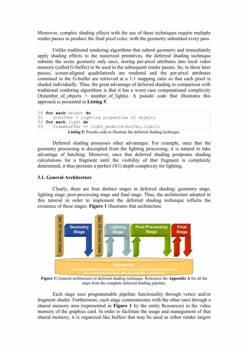
Clearly, there are four distinct stages in deferred shading: geometry stage, lighting stage, post-processing stage and final stage. Thus, the architecture adopted in this tutorial in order to implement the deferred shading technique reflects the existence of these stages. Figure 1 illustrates that architecture.

ResourcesMain frame buffer (color only), G-buffer (color, depth, aux0 and aux1) and

four color only P-buffers (two full and two ¼ resolution)

GeometryStage

LightingStage

Post-ProcessingStage

Final Stage

Set 3D

Render S

tate

Set 2D

Render S

tate





GeometryStage

LightingStage


Final Stage

Set 3D

Render S

tate

Set 2D

Render S

tate

GeometryStage

LightingStage


Final Stage

Set 3D

Render S

tate

Set 2D

Render S

tate

Figure 1: General architecture of deferred shading technique. Reference the Appendix A for all the steps from the complete deferred shading pipeline.

Each stage uses programmable pipeline functionality through vertex and/or fragment shader. Furthermore, each stage communicates with the other ones through a shared memory area (represented in Figure 1 by the entity Resources) in the video memory of the graphics card. In order to facilitate the usage and management of that shared memory, it is organized like buffers that may be used as either render targets

(when a stage writes information into the video memory) or textures (when a stage reads information from the video memory).

The geometry stage implements a perspective projection camera, in three-dimensional space, and it is responsible for feeding the G-buffer with information to be used in the next stages. All subsequent stages operate in image-space and work with an orthographic projection camera using screen resolution dimensions. The lighting stage receives as input the contents of the G-buffer as well as light sources information and it accumulates lighting into a full resolution P-buffer (defined in Section 3.2). In the next stage, some post-processing passes are performed in order to enhance the image generated in the previous stage. Finally, the enhanced image is transferred to the main frame buffer in order to be displayed on the screen.

In the following sections, each of these stages as well as all resources required to accomplish the deferred shading technique will be presented in more detail.

3.2. Resources

As described in Section 3.1, the exchange of information among the deferred shading stages involves the ability to render information into the graphics card's video memory and later to use it as a texture. Moreover, that kind of task must be executed as efficiently as possible in order to maintain all processing real time. Thus, it is extremely important to render to the graphics card's video memory directly and use the resulting image as a texture without requiring a buffer to texture copy. It may be done through the use of a special off-screen buffer, also called pixel buffer (P-buffer for short), available in OpenGL through the extensions WGL_ARB_render_texture [Poddar01] and WGL_ARB_pbuffer [Kirkland02].

All P-buffers referenced in this tutorial can be used as render targets or textures, but they cannot be used as both types at the same time (i.e., cannot be read from and write to at the same time). The G-buffer is a special P-buffer containing not only color, but depth and two extra auxiliary buffers. In order to write to all its buffers, it would require rendering one pass per buffer. However, if the current graphics card supports Multiple Render Targets (MRT) capability, it is possible to write to all buffers in a single pass. In OpenGL, it may be performed through the extension GL_ATI_draw_buffers [Mace02], that supports writing to up to four render targets simultaneously.

In order to exemplify the implementation of the deferred shading technique, the general architecture illustrated in Figure 1 will be represented by the class pDeferredShader. The first attributes of that class are the G-buffer and the four P-buffers, each represented by the class pPBuffer available through the middle-ware P3D [Policarpo05]; and the first methods of that class allow the management of these buffers as render targets or textures as shown at Listing 6.

00 class pDeferredShader01 {02 pPBuffer *m_mrt; // G-buffer03 unsigned int m_mrttex[4]; // G-buffer texture ids04 05 pPBuffer *m_fb[4]; // P-buffers06 unsigned int m_fbtex[4]; // P-buffers texture ids

07 08 // G-buffer management09 void mrt_bind_render();10 void mrt_unbind_render();11 void mrt_bind_texture(int target);12 void mrt_unbind_texture(int target);13 14 // P-buffer management15 void fb_bind_render(int buffer);16 void fb_unbind_render(int buffer);17 void fb_bind_texture(int buffer,int texunit);18 void fb_unbind_texture(int buffer,int texunit);19 ...20 };

Listing 6: Attributes and methods used to manage the G-buffer and the four P-buffers.

In order to use a P-buffer as an off-screen render target, one of the available “bind_render” methods must be called. Once that the P-buffer was filled in with some information it may be released through one of the available “unbind_render” methods.Similarly, to use a P-buffer as a texture, one of the available “bind_texture” methods must be called and after its usage one of the available “unbind_texture” methods must be called. It is important to remember that it is not allowed to bind a buffer as texture if it is already bound as a render target and vice-versa.

3.3. Geometry Stage

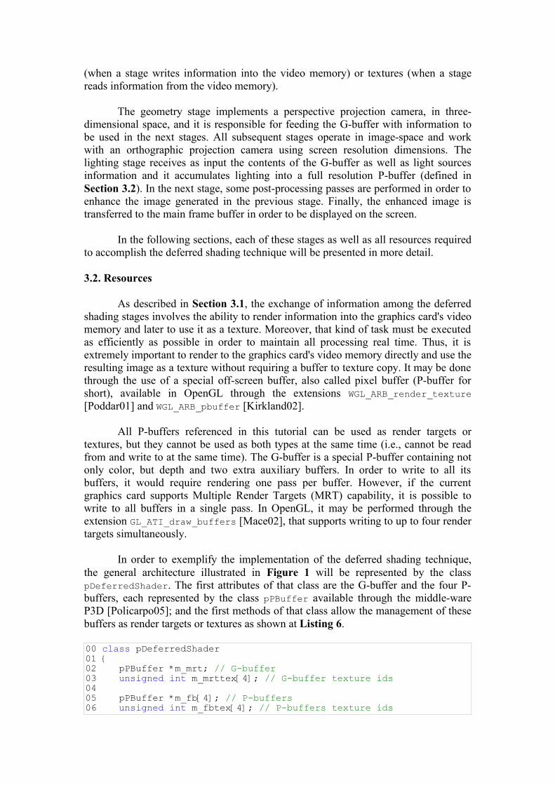
The geometry stage is the only stage that actually uses 3D geometric data. Thus, the input of that stage is the mesh of the scene to be rendered and the output is the G-buffer filled in with information required to shade all pixels that contribute to the final image. Figure 2 illustrates the process and necessary resources to perform it.

Geometry Stage

Bind G-buffer for Rendering

Draw Depth Pass

Draw Material Pass

Unbind G-buffer

G-bufferdepthcolor aux0 aux1

normal depth diffuse specular

Geometry Stage


Draw Depth Pass

Draw Material Pass

Unbind G-buffer

Geometry Stage


Draw Depth Pass

Draw Material Pass

Unbind G-buffer



G-bufferdepthdepthcolorcolor aux0aux0 aux1aux1


Figure 2: Geometry stage of deferred shading general architecture.

In order to fill the G-buffer with the required information, it is necessary to set the G-buffer as the current render target. It may be performed through the method mrt_bind_render(), available in the class pDeferredShader (see Listing 6). Once that the G-buffer is ready to receive data, the scene may be rendered. Firstly, raw geometry information (only vertices without normals, texture coordinates and materials) is sent to the graphics card using the fixed function pipeline which only updates the G-buffer's depth buffer. Next, material and geometric information of the scene are sent to the graphics card and a fragment shader is responsible for filling the

rest of the G-buffer's data. Finally, the G-buffer can be unbound calling the method mrt_unbind_render(). The method that implements the geometry stage in shown at Listing 7.

00 void pDeferredShader::geometry_stage(pMesh *scene)01 {02 // bind G-buffer for rendering03 mrt_bind_render();04 // perspective camera model05 set_perspective_camera();06 // OpenGL render states configuration07 glCullFace(GL_BACK);08 glEnable(GL_CULL_FACE);09 glDisable(GL_BLEND);10 glDepthFunc(GL_LEQUAL);11 glEnable(GL_DEPTH_TEST);12 glDisable(GL_TEXTURE_2D);13 glColor4f(1.0f,1.0f,1.0f,1.0f);14 glClearColor(bgcolor.x,bgcolor.y,bgcolor.z,1.0);15 glClearDepth(1.0);16 glColorMask(true,true,true,true);17 glDepthMask(true);18 glClear(GL_DEPTH_BUFFER_BIT|GL_COLOR_BUFFER_BIT);19 // send raw scene geometry that updates the depth buffer20 draw_depth(scene);21 // fill the G-buffer with lighting attributes and materials 22 draw_material(scene);23 // unbind the G-buffer24 mrt_unbind_render();25 }

Listing 7: Code to implement the geometry stage of the deferred shading technique.

At line 3 the G-buffer is set as the current render target. So, at line 5 a perspective camera model is defined according to the current viewer. From line 7 to 18 some render states are defined and the color and depth buffers are cleared. Next, at line 20 the raw scene geometry updates the depth buffer and at line 22 material information about the scene is sent to the G-buffer. Finally, at line 24, the main frame buffer becomes the current render target again.

3.3.1. Depth Pass

The approach of using a depth only phase first in order to optimize the next phases was used in Doom3 [Carmack]. The idea is to use the depth buffer to determine the closest surface at each pixel and then only executes more complex processing from the material shader for pixels passing the depth test. That approach is called early Z culling and all pixels failing the depth test will be discarded before their material shader is executed. The depth only pass is shown at Listing 8.

00 void pDeferredShader::draw_depth(pMesh *scene)01 {02 glColorMask(false,false,false,false);03 glDepthMask(true);0405 // draw raw scene geometry06 scene->array_lock(VERTICES);07 scene->array_draw();08 scene->array_unlock();09 10 glColorMask(true,true,true,true);

11 glDepthMask(false);12 }

Listing 8: Code to implement a depth only phase during the execution of the deferred shading technique.

3.3.2. Material Pass

The objective of the material pass is to fill the G-buffer with all necessary per-pixel lighting terms in order to evaluate the Equation 1. Thus, the G-buffer must contain information like position, surface normal, diffuse color, specular color and shininess. However, once that the G-buffer is represented as a P-buffer with multiple render targets capability, it is necessary to specify a way to organize all these information together.

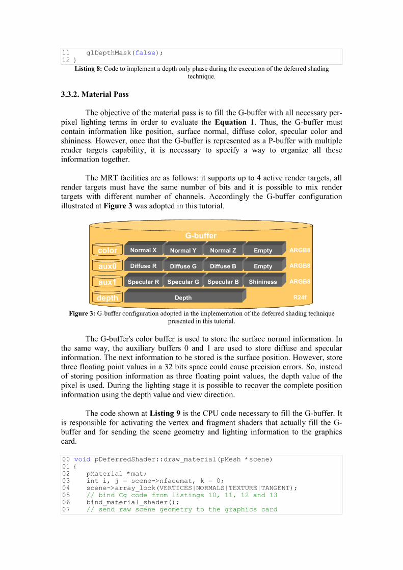
The MRT facilities are as follows: it supports up to 4 active render targets, all render targets must have the same number of bits and it is possible to mix render targets with different number of channels. Accordingly the G-buffer configuration illustrated at Figure 3 was adopted in this tutorial.

G-buffer

Specular R

Depth

ARGB8

ARGB8

ARGB8

R24fdepth

color

aux0

aux1 Specular G Specular B Shininess

Diffuse R Diffuse G Diffuse B Empty

Normal X Normal Y Normal Z Empty

G-bufferG-buffer

Specular R

Depth

ARGB8

ARGB8

ARGB8

R24fdepthdepth

colorcolor

aux0aux0

aux1aux1 Specular G Specular B Shininess

Diffuse R Diffuse G Diffuse B Empty

Normal X Normal Y Normal Z Empty

Figure 3: G-buffer configuration adopted in the implementation of the deferred shading technique presented in this tutorial.

The G-buffer's color buffer is used to store the surface normal information. In the same way, the auxiliary buffers 0 and 1 are used to store diffuse and specular information. The next information to be stored is the surface position. However, store three floating point values in a 32 bits space could cause precision errors. So, instead of storing position information as three floating point values, the depth value of the pixel is used. During the lighting stage it is possible to recover the complete position information using the depth value and view direction.

The code shown at Listing 9 is the CPU code necessary to fill the G-buffer. It is responsible for activating the vertex and fragment shaders that actually fill the G-buffer and for sending the scene geometry and lighting information to the graphics card.

00 void pDeferredShader::draw_material(pMesh *scene)01 {02 pMaterial *mat;03 int i, j = scene->nfacemat, k = 0;04 scene->array_lock(VERTICES|NORMALS|TEXTURE|TANGENT); 05 // bind Cg code from listings 10, 11, 12 and 1306 bind_material_shader();07 // send raw scene geometry to the graphics card

08 for( i=0;i<j;i++ )09 {10 mat = &scene->mat[scene->face[k].material];11 if (mat->bump == 0 || mat->texnormalid == -1)12 {13 set_material_shader_params(mat->diffuse,mat->specular,1,14 mat->texid,mat->texnormalid);15 glDrawElements(GL_TRIANGLES,3*m->facemat[i],16 GL_UNSIGNED_INT,(void *)(k*3*sizeof(unsigned int)));17 }18 k += m->facemat[i];19 }20 // unbind Cg code from listings 10, 11, 12 and 1321 unbind_material_shader();22 scene->array_unlock();23 }

Listing 9: Code to implement the material pass of the geometry stage.

The vertex shader of the material pass is used to transform all geometric information to view space and to output it to the fragment shader as shown at Listing 10.

00 // application to vertex shader01 struct a2v 02 {03 float4 pos : POSITION; // position (object space)04 float3 normal : NORMAL; // normal (object space)05 float2 texcoord : TEXCOORD0; // texture coordinates06 float3 tangent : TEXCOORD1; // tangent vector07 float3 binormal : TEXCOORD2; // binormal vector08 };0910 // vertex shader to fragment shader11 struct v2f12 {13 float4 hpos : POSITION; // position (clip space)14 float2 texcoord : TEXCOORD0; // texture coordinate15 float3 vpos : TEXCOORD1; // position (view space)16 float3 normal : TEXCOORD2; // surface normal (view space)17 float3 tangent : TEXCOORD3; // tangent vector (view space)18 float3 binormal : TEXCOORD4; // binormal vector (view space)19 };2021 // vertex shader22 v2f view_space(a2v IN)23 {24 v2f OUT;25 // vertex position in object space26 float4 pos = float4(IN.pos.x,IN.pos.y,IN.pos.z,1.0);27 // vertex position in clip space28 OUT.hpos = mul(glstate.matrix.mvp,pos);29 // copy texture coordinates30 OUT.texcoord = IN.texcoord.xy;31 // compute modelview rotation only part32 float3x3 modelviewrot = float3x3(glstate.matrix.modelview[0]);33 // vertex position in view space (with model transformations)34 OUT.vpos = mul(glstate.matrix.modelview[0],pos).xyz;35 // tangent space vectors in view space (with model 36 // transformations)37 OUT.normal = mul(modelviewrot,IN.normal);38 OUT.tangent = mul(modelviewrot,IN.tangent);39 OUT.binormal = mul(modelviewrot,IN.binormal);40 return OUT;

41 }Listing 10: Vertex shader of the material pass in order to transform all geometric information to view

space and to output it to the fragment shader.

As described previously, instead of storing position information as three floating point values, the normalized depth value of the pixel in the range [0,1] is stored. So, it is necessary to bind the depth buffer as a texture. Graphics cards that support the OpenGL extension WGL_NV_render_depth_texture [Brown03] may use this capability allowing the depth buffer to be used for both rendering and texturing. On graphics cards that do not support that extension, it is necessary to calculate the depth value in the fragment shader and to convert it to a color (3 times 8 bits integer). It may be done with the following helper function as shown in Listing 11.

00 float3 float_to_color(in float f)01 {02 float3 color;03 f *= 256;04 color.x = floor(f);05 f = (f-color.x)*256;06 color.y = floor(f);07 color.z = f-color.y;08 color.xy *= 0.00390625; // *= 1.0/25609 return color;10 }

Listing 11: Helper function that converts depth information to a color (3x8 bits integer).

The fragment shader of the material pass is the function that really stores all lighting information into the G-buffer. It is performed through the filling of the structure f2s_mrt that represents a cell in the G-buffer as shown at Listing 12.

00 struct f2s_mrt01 {02 float3 color0 : COLOR0; // normal (color buffer)03 float3 color1 : COLOR1; // diffuse (auxiliary buffer 0)04 float4 color2 : COLOR2; // specular (auxiliary buffer 1)05 #ifndef NV_RENDER_DEPTH_TEXTURE06 float3 color3 : COLOR3; // depth (auxiliary buffer 2)07 #endif08 };

Listing 12: Output structure from fragment shader of the material pass to the G-buffer.

Finally, in Listing 13, the fragment shader that fills the structure f2s_mrt is presented.

00 f2s_mrt mrt_normal(01 v2f IN, // input from the vertex shader02 uniform sampler2D normaltex : TEXUNIT0, // normal texture map 03 uniform sampler2D colortex : TEXUNIT1, // color texture map 04 uniform float4 diffuse, // diffuse color05 uniform float4 specular, // specular color06 uniform float2 planes, // near and far plane information07 uniform float tile) // tile factor08 {09 f2s_mrt OUT;1011 float2 txcoord = IN.texcoord*tile;12 // normal map13 float3 normal = f3tex2D(normaltex,txcoord);

14 // color map15 float3 color = f3tex2D(colortex,txcoord);16 // transform normal to view space17 normal -= 0.5;18 normal = normalize(normal.x*IN.tangent + normal.y*IN.binormal 19 + normal.z*IN.normal);20 // convert normal back to [0,1] color space21 normal = normal*0.5+0.5;22 // fill G-buffer23 OUT.color0 = normal;24 OUT.color1 = color*diffuse.xyz;25 OUT.color2 = specular;26 #ifndef NV_RENDER_DEPTH_TEXTURE27 float d=((planes.x*IN.vpos.z+planes.y)/-IN.vpos.z); // detph28 OUT.color3 = float_to_color(d);29 #endif30 return OUT;31 }

Listing 13: Fragment shader of the material pass in order to fill the G-buffer.

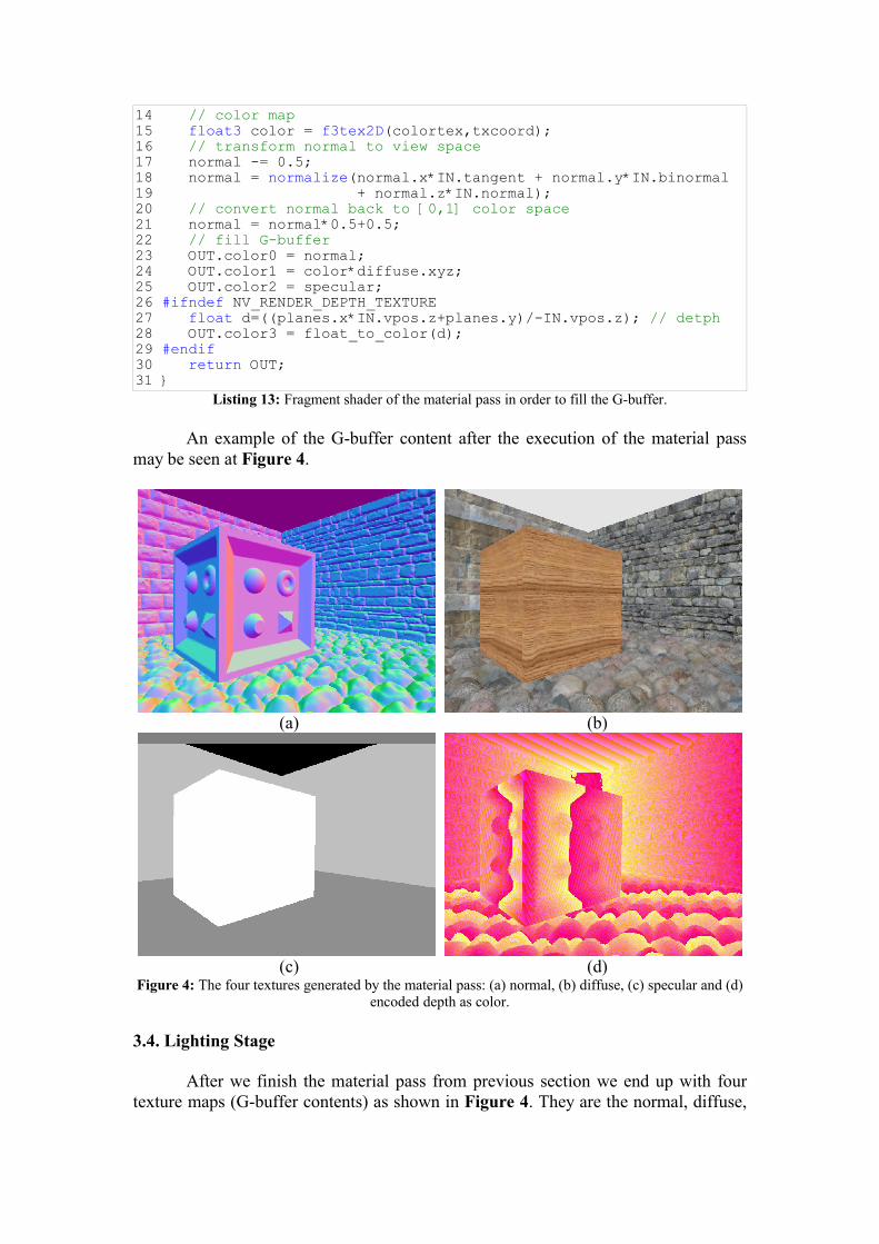
An example of the G-buffer content after the execution of the material pass may be seen at Figure 4.

(a) (b)

(c) (d)Figure 4: The four textures generated by the material pass: (a) normal, (b) diffuse, (c) specular and (d)

encoded depth as color.

3.4. Lighting Stage

After we finish the material pass from previous section we end up with four texture maps (G-buffer contents) as shown in Figure 4. They are the normal, diffuse,

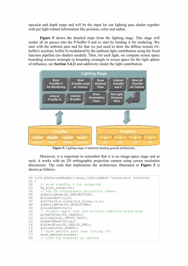
specular and depth maps and will be the input for our lighting pass shader together with per light related information like position, color and radius.

Figure 5 shows the detailed steps from the lighting stage. This stage will render all its passes into the P-buffer 0 and so start by binding it for rendering. We start with the ambient pass and for that we just need to draw the diffuse texture (G-buffer's auxiliary buffer 0) modulated by the ambient light contribution using the fixed function pipeline (no shaders needed). Then, for each light, we compute screen space bounding scissors rectangle (a bounding rectangle in screen space for the light sphere of influence, see Section 3.4.2) and additively render the light contribution.

Lighting Stage

Bind P-buffer 0

for Rendering

Bind G-buffer aux0

as Texture

Draw Ambient

Pass

UnbindG-buffer aux 0

Bind allG-buffer

as Texture

Set LightScissors

Rect

DrawIllumination

Pass

UnbindG-buffer

Unbind P-buffer 0



P-buffers

10 2 3full full 1/4 1/4

Lighting Stage

Bind P-buffer 0

for Rendering

Bind G-buffer aux0

as Texture

Draw Ambient

Pass


Bind allG-buffer

as Texture

Set LightScissors

Rect

DrawIllumination

Pass

UnbindG-buffer

Unbind P-buffer 0

Lighting Stage

Bind P-buffer 0

for Rendering

Bind G-buffer aux0

as Texture

Draw Ambient

Pass


Bind allG-buffer

as Texture

Set LightScissors

Rect

DrawIllumination

Pass

UnbindG-buffer

Unbind P-buffer 0



P-buffers

10 2 3full full 1/4 1/4





G-bufferdepthdepthcolorcolor aux0aux0 aux1aux1


P-buffers

10 2 3full full 1/4 1/4

P-buffers

10 2 3full full 1/4 1/4

P-buffers

1100 22 33full full 1/4 1/4

Figure 5: Lighting stage of deferred shading general architecture.

Moreover, it is important to remember that it is an image-space stage and as such, it works with an 2D orthographic projection camera using screen resolution dimensions. The code that implements the architecture illustrated at Figure 5 is shown as follows.

00 void pDeferredShader::draw_lights(pMesh *scene,bool scissors)01 {02 // bind P-buffer 0 for rendering03 fb_bind_render(0);04 // set 2D orthographic projection camera05 glMatrixMode(GL_PROJECTION);06 glLoadIdentity();07 glOrtho(0,m_sizex,0,m_sizey,-1,1);08 glMatrixMode(GL_MODELVIEW);09 glLoadIdentity();10 // disable depth test and activate additive blend mode11 glDepthFunc(GL_LEQUAL);12 glDisable(GL_DEPTH_TEST);13 glDepthMask(false);14 glBlendFunc(GL_ONE,GL_ONE);15 glDisable(GL_BLEND);16 // draw ambient pass (see listing 15)17 draw_ambient(scene);18 // bind the G-buffer as texture

19 mrt_bind_texture(ALL);20 // draw lighting pass (see listing 17)21 draw_lighting(scene,scissors);22 // unbind the G-buffer23 mrt_unbind_texture(ALL);24 // unbind the P-buffer 025 fb_unbind_render(0);26 }

Listing 14: Code to implement the lighting stage of the deferred shading technique.

In this way, we achieve the main advantage of the deferred shading technique - we totally separate lighting from geometry. A complicated feature of most direct rendering engines is how to compute the geometry sets associated to each light. For dynamic lights and dynamic geometry this computation can be complex and require testing all geometry for containment by the light volumes (sphere, bounding box or frustum containment tests). This requires more elaborate geometry organization like hierarchical representations or tree structures in order to make such dynamic sets real-time.

When using deferred shading we do not need to know what geometry is illuminated by what light and could just process all lights we find visible to the viewer. While we traverse the scene for visible geometry we simply store the lights we find on the way (so lights do NOT need to know which geometry they will influence). We can also use view culling applied to the light volumes and some type of occlusion culling to try to reduce the number of lights we need to render.

As with direct rendering, we can add together the contribution for each light executing one pass per light source or have a more complex shader handling multiple lights at once. Using one pass per light allow us to do shadows (based on stencil or shadow map) but will be less efficient than processing multiple lights in a single pass. Another thing we must consider is the scissors optimization possible with the one pass per light approach (explained in Section 3.4.2). For example in a scene with many small lights, each taking a small area of the screen pixels, scissors optimization would work optimally and would be as efficient as processing all lights in a single pass.

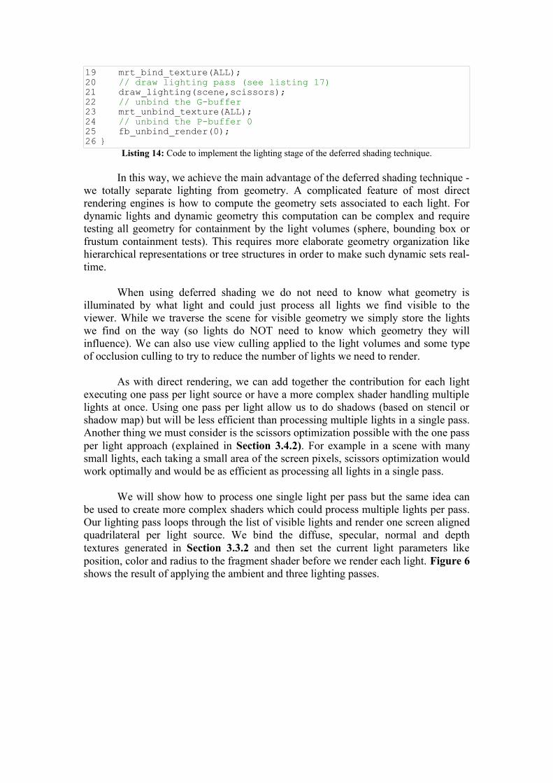
We will show how to process one single light per pass but the same idea can be used to create more complex shaders which could process multiple lights per pass. Our lighting pass loops through the list of visible lights and render one screen aligned quadrilateral per light source. We bind the diffuse, specular, normal and depth textures generated in Section 3.3.2 and then set the current light parameters like position, color and radius to the fragment shader before we render each light. Figure 6 shows the result of applying the ambient and three lighting passes.

Figure 6: Final image generated from textures in Figure 4 after the lighting and post-processing passes.

3.4.1. Ambient Pass

The ambient pass initializes all the pixels in the buffer we are going to use to accumulate lighting (P-buffer 0 from Figure 5). This way, pixels without any illumination will have only the ambient contribution. For that, all we need to do is to render the diffuse texture (from Figure 4b) modulated by the current ambient light factor. The code for the ambient pass is shown at Listing 15.

00 void pDeferredShader::draw_ambient(pMesh *scene)01 {02 // set ambient color to be modulated with diffuse material03 glColor4fv(&scene->ambient.x);04 // bind diffuse G-buffer's auxiliary 005 mrt_bind_texture(AUX0);06 // draw screen-aligned quadrilateral07 draw_rect(0,0,m_sizex,m_sizey);08 // unbind diffuse G-buffer's auxiliary 009 mrt_unbind_texture(AUX0);10 }

Listing 15: Code to implement the ambient pass.

3.4.2. Light Scissors Optimization

When rendering the lighting pass for a single light, a good optimization to use is the scissors rectangle. Rendering a full screen quadrilateral polygon to perform lighting will execute the lighting shader for all pixels in the buffer, but depending on the light illumination radius, some pixels might be outside of light sphere of influence thus receiving no light contribution. We can save a lot of computation by calculating the bounding rectangle in screen space for the light sphere of influence and enabling the scissors test. When enabled, all fragments outside the scissors rectangle will be discarded before the fragment shader is executed saving a lot of processing.

In our test scene we have three light sources but depending on the viewer position some of them can project to a small area in screen. For example, using a 512x512 buffer (256M pixels) we would need to execute the fragment shader 768M times to process three lights without scissors optimization. But using scissors optimization we reduce the number of pixels processed per light and on average save

50% of the fragments. Of course this will depend on the light positions and radius and in some cases we might have all lights taking all screen space.

The scissors rectangle computation is done on the CPU before we render each light source. One possible simple solution to compute the scissors rectangle would be to project each of the eight light bounding box vertices into screen space and finding the enclosing 2D rectangle for those points. But this will generate a larger rectangle than needed and might fail in cases where some of the vertices are behind the viewer.

A better solution is to find the planes parallel to the view frustum which are tangent to the light's sphere of influence. Listing 16 shows the full source code for calculating the scissors rectangle for a given light with position and radius (stored in light position W component). More details about how this is achived can be found on [Lengyel03] or at http://www.gamasutra.com/features/20021011/lengyel_06.htm.

000 int pDeferredShader::set_light_scissor(const pVector& lightpos, 000 int sx,int sy)001 {002 int rect[4]={ 0,0,sx,sy };003 float d;004005 float r=lightpos.w;006 float r2=r*r;007008 pVector l=lightpos;009 pVector l2=lightpos*lightpos;010011 float e1=1.2f;012 float e2=1.2f*g_render->aspect;013014 d=r2*l2.x - (l2.x+l2.z)*(r2-l2.z);015 if (d>=0)016 {017 d=sqrtf(d);018019 float nx1=(r*l.x + d)/(l2.x+l2.z);020 float nx2=(r*l.x - d)/(l2.x+l2.z);021022 float nz1=(r-nx1*l.x)/l.z;023 float nz2=(r-nx2*l.x)/l.z;024025 float e=1.25f;026 float a=g_render->aspect;027028 float pz1=(l2.x+l2.z-r2)/(l.z-(nz1/nx1)*l.x);029 float pz2=(l2.x+l2.z-r2)/(l.z-(nz2/nx2)*l.x);030031 if (pz1<0)032 {033 float fx=nz1*e1/nx1;034 int ix=(int)((fx+1.0f)*sx*0.5f);035036 float px=-pz1*nz1/nx1;037 if (px<l.x)038 rect[0]=max(rect[0],ix);039 else040 rect[2]=min(rect[2],ix);041 }042043 if (pz2<0)044 {

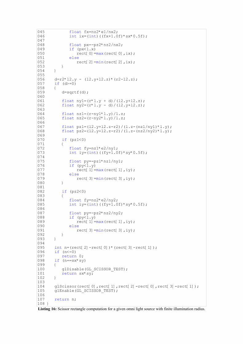
045 float fx=nz2*e1/nx2;046 int ix=(int)((fx+1.0f)*sx*0.5f);047048 float px=-pz2*nz2/nx2;049 if (px<l.x)050 rect[0]=max(rect[0],ix);051 else052 rect[2]=min(rect[2],ix);053 }054 }055056 d=r2*l2.y - (l2.y+l2.z)*(r2-l2.z);057 if (d>=0)058 {059 d=sqrtf(d);060061 float ny1=(r*l.y + d)/(l2.y+l2.z);062 float ny2=(r*l.y - d)/(l2.y+l2.z);063064 float nz1=(r-ny1*l.y)/l.z;065 float nz2=(r-ny2*l.y)/l.z;066067 float pz1=(l2.y+l2.z-r2)/(l.z-(nz1/ny1)*l.y);068 float pz2=(l2.y+l2.z-r2)/(l.z-(nz2/ny2)*l.y);069070 if (pz1<0)071 {072 float fy=nz1*e2/ny1;073 int iy=(int)((fy+1.0f)*sy*0.5f);074075 float py=-pz1*nz1/ny1;076 if (py<l.y)077 rect[1]=max(rect[1],iy);078 else079 rect[3]=min(rect[3],iy);080 }081082 if (pz2<0)083 {084 float fy=nz2*e2/ny2;085 int iy=(int)((fy+1.0f)*sy*0.5f);086087 float py=-pz2*nz2/ny2;088 if (py<l.y)089 rect[1]=max(rect[1],iy);090 else091 rect[3]=min(rect[3],iy);092 }093 }094095 int n=(rect[2]-rect[0])*(rect[3]-rect[1]);096 if (n<=0)097 return 0;098 if (n==sx*sy)099 {100 glDisable(GL_SCISSOR_TEST);101 return sx*sy;102 }103104 glScissor(rect[0],rect[1],rect[2]-rect[0],rect[3]-rect[1]);105 glEnable(GL_SCISSOR_TEST);106107 return n;108 }Listing 16: Scissor rectangle computation for a given omni light source with finite illumination radius.

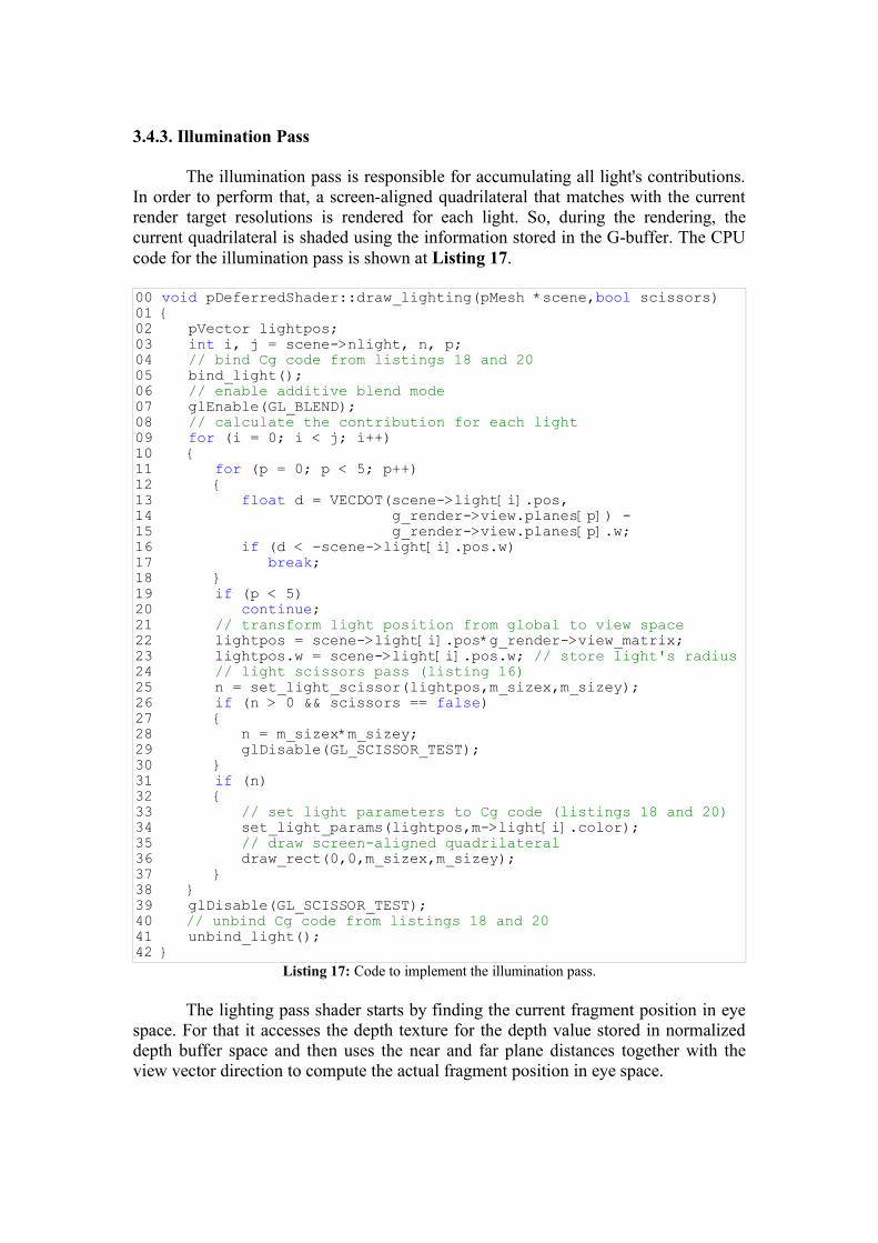
3.4.3. Illumination Pass

The illumination pass is responsible for accumulating all light's contributions. In order to perform that, a screen-aligned quadrilateral that matches with the current render target resolutions is rendered for each light. So, during the rendering, the current quadrilateral is shaded using the information stored in the G-buffer. The CPU code for the illumination pass is shown at Listing 17.

00 void pDeferredShader::draw_lighting(pMesh *scene,bool scissors)01 {02 pVector lightpos;03 int i, j = scene->nlight, n, p;04 // bind Cg code from listings 18 and 2005 bind_light();06 // enable additive blend mode07 glEnable(GL_BLEND);08 // calculate the contribution for each light09 for (i = 0; i < j; i++)10 {11 for (p = 0; p < 5; p++)12 {13 float d = VECDOT(scene->light[i].pos,14 g_render->view.planes[p]) -15 g_render->view.planes[p].w;16 if (d < -scene->light[i].pos.w)17 break;18 }19 if (p < 5)20 continue;21 // transform light position from global to view space22 lightpos = scene->light[i].pos*g_render->view_matrix;23 lightpos.w = scene->light[i].pos.w; // store light's radius24 // light scissors pass (listing 16)25 n = set_light_scissor(lightpos,m_sizex,m_sizey);26 if (n > 0 && scissors == false)27 {28 n = m_sizex*m_sizey;29 glDisable(GL_SCISSOR_TEST);30 }31 if (n)32 {33 // set light parameters to Cg code (listings 18 and 20)34 set_light_params(lightpos,m->light[i].color);35 // draw screen-aligned quadrilateral36 draw_rect(0,0,m_sizex,m_sizey);37 }38 }39 glDisable(GL_SCISSOR_TEST);40 // unbind Cg code from listings 18 and 2041 unbind_light();42 }

Listing 17: Code to implement the illumination pass.

The lighting pass shader starts by finding the current fragment position in eye space. For that it accesses the depth texture for the depth value stored in normalized depth buffer space and then uses the near and far plane distances together with the view vector direction to compute the actual fragment position in eye space.

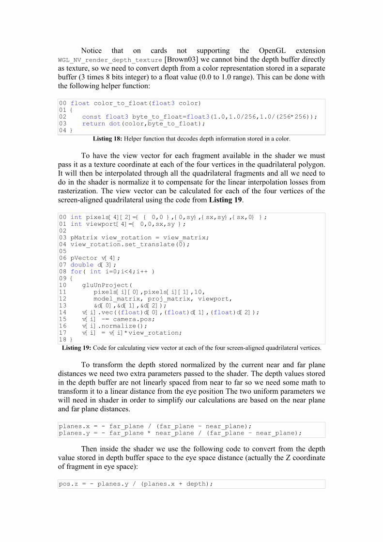
Notice that on cards not supporting the OpenGL extension WGL_NV_render_depth_texture [Brown03] we cannot bind the depth buffer directly as texture, so we need to convert depth from a color representation stored in a separate buffer (3 times 8 bits integer) to a float value (0.0 to 1.0 range). This can be done with the following helper function:

00 float color_to_float(float3 color)01 {02 const float3 byte_to_float=float3(1.0,1.0/256,1.0/(256*256));03 return dot(color,byte_to_float);04 }

Listing 18: Helper function that decodes depth information stored in a color.

To have the view vector for each fragment available in the shader we must pass it as a texture coordinate at each of the four vertices in the quadrilateral polygon. It will then be interpolated through all the quadrilateral fragments and all we need to do in the shader is normalize it to compensate for the linear interpolation losses from rasterization. The view vector can be calculated for each of the four vertices of the screen-aligned quadrilateral using the code from Listing 19.

00 int pixels[4][2]={ { 0,0 },{0,sy},{sx,sy},{sx,0} };01 int viewport[4]={ 0,0,sx,sy };0203 pMatrix view_rotation = view_matrix;04 view_rotation.set_translate(0);0506 pVector v[4];07 double d[3];08 for( int i=0;i<4;i++ )09 {10 gluUnProject(11 pixels[i][0],pixels[i][1],10,12 model_matrix, proj_matrix, viewport,13 &d[0],&d[1],&d[2]);14 v[i].vec((float)d[0],(float)d[1],(float)d[2]);15 v[i] -= camera.pos;16 v[i].normalize();17 v[i] = v[i]*view_rotation;18 }Listing 19: Code for calculating view vector at each of the four screen-aligned quadrilateral vertices.

To transform the depth stored normalized by the current near and far plane distances we need two extra parameters passed to the shader. The depth values stored in the depth buffer are not linearly spaced from near to far so we need some math to transform it to a linear distance from the eye position The two uniform parameters we will need in shader in order to simplify our calculations are based on the near plane and far plane distances.

planes.x = - far_plane / (far_plane – near_plane);planes.y = - far_plane * near_plane / (far_plane – near_plane);

Then inside the shader we use the following code to convert from the depth value stored in depth buffer space to the eye space distance (actually the Z coordinate of fragment in eye space):

pos.z = - planes.y / (planes.x + depth);

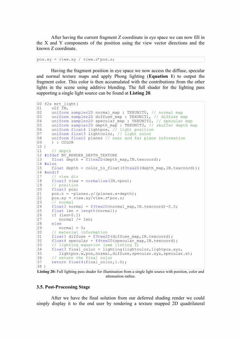
After having the current fragment Z coordinate in eye space we can now fill in the X and Y components of the position using the view vector directions and the known Z coordinate.

pos.xy = view.xy / view.z*pos.z;

Having the fragment position in eye space we now access the diffuse, specular and normal texture maps and apply Phong lighting (Equation 1) to output the fragment color. This color is then accumulated with the contributions from the other lights in the scene using additive blending. The full shader for the lighting pass supporting a single light source can be found at Listing 20.

00 f2s mrt_light(01 v2f IN,02 uniform sampler2D normal_map : TEXUNIT0, // normal map 03 uniform sampler2D diffuse_map : TEXUNIT1, // diffuse map 04 uniform sampler2D specular_map : TEXUNIT2, // specular map 05 uniform sampler2D depth_map : TEXUNIT3, // zbuffer depth map06 uniform float4 lightpos, // light position07 uniform float3 lightcolor, // light color08 uniform float2 planes // near and far plane information09 ) : COLOR10 {11 // depth12 #ifdef NV_RENDER_DEPTH_TEXTURE13 float depth = f1tex2D(depth_map,IN.texcoord);14 #else15 float depth = color_to_float(f3tex2D(depth_map,IN.texcoord));16 #endif17 // view dir18 float3 view = normalize(IN.vpos);19 // position20 float3 pos;21 pos.z = -planes.y/(planes.x+depth);22 pos.xy = view.xy/view.z*pos.z;23 // normal24 float3 normal = f3tex2D(normal_map,IN.texcoord)-0.5;25 float len = length(normal);26 if (len>0.1)27 normal /= len;28 else29 normal = 0;30 // material information31 float3 diffuse = f3tex2D(diffuse_map,IN.texcoord);32 float4 specular = f4tex2D(specular_map,IN.texcoord);33 // lighting equation (see listing 2)34 float3 final_color = lighting(lightcolor,lightpos.xyz,35 lightpos.w,pos,normal,diffuse,specular.xyz,specular.w);36 // return the final color37 return float4(final_color,1.0);38 }Listing 20: Full lighting pass shader for illumination from a single light source with position, color and

attenuation radius.

3.5. Post-Processing Stage

After we have the final solution from our deferred shading render we could simply display it to the end user by rendering a texture mapped 2D quadrilateral

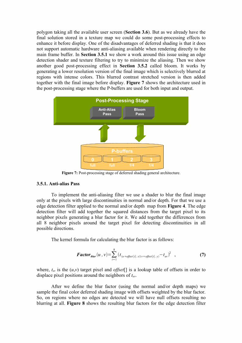
polygon taking all the available user screen (Section 3.6). But as we already have the final solution stored in a texture map we could do some post-processing effects to enhance it before display. One of the disadvantages of deferred shading is that it does not support automatic hardware anti-aliasing available when rendering directly to the main frame buffer. In Section 3.5.1 we show a work around this issue using an edge detection shader and texture filtering to try to minimize the aliasing. Then we show another good post-processing effect in Section 3.5.2 called bloom. It works by generating a lower resolution version of the final image which is selectively blurred at regions with intense colors. This blurred contrast stretched version is then added together with the final image before display. Figure 7 shows the architecture used in the post-processing stage where the P-buffers are used for both input and output.

Post-Processing Stage

Anti-Alias Pass

Bloom Pass

P-buffers

10 2 3full full 1/4 1/4


Anti-Alias Pass

Bloom Pass


Anti-Alias Pass

Bloom Pass

P-buffers

10 2 3full full 1/4 1/4

P-buffers

1100 22 33full full 1/4 1/4

Figure 7: Post-processing stage of deferred shading general architecture.

3.5.1. Anti-alias Pass

To implement the anti-aliasing filter we use a shader to blur the final image only at the pixels with large discontinuities in normal and/or depth. For that we use a edge detection filter applied to the normal and/or depth map from Figure 4. The edge detection filter will add together the squared distances from the target pixel to its neighbor pixels generating a blur factor for it. We add together the differences from all 8 neighbor pixels around the target pixel for detecting discontinuities in all possible directions.

The kernel formula for calculating the blur factor is as follows:

Factorblur u ,v=∑i=1

8

t uoffset [i] . xvoffset [i] . y−tuv 2 , (7)

where, tuv is the (u,v) target pixel and offset[] is a lookup table of offsets in order to displace pixel positions around the neighbors of tuv.

After we define the blur factor (using the normal and/or depth maps) we sample the final color deferred shading image with offsets weighted by the blur factor. So, on regions where no edges are detected we will have null offsets resulting no blurring at all. Figure 8 shows the resulting blur factors for the edge detection filter

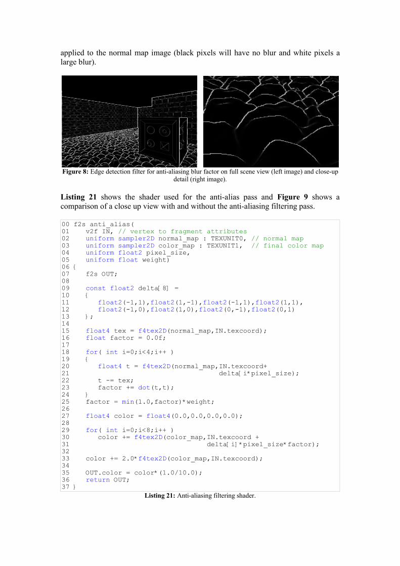
applied to the normal map image (black pixels will have no blur and white pixels a large blur).

Figure 8: Edge detection filter for anti-aliasing blur factor on full scene view (left image) and close-up detail (right image).

Listing 21 shows the shader used for the anti-alias pass and Figure 9 shows a comparison of a close up view with and without the anti-aliasing filtering pass.

00 f2s anti_alias(01 v2f IN, // vertex to fragment attributes02 uniform sampler2D normal_map : TEXUNIT0, // normal map03 uniform sampler2D color_map : TEXUNIT1, // final color map04 uniform float2 pixel_size,05 uniform float weight)06 {07 f2s OUT;0809 const float2 delta[8] =10 { 11 float2(-1,1),float2(1,-1),float2(-1,1),float2(1,1), 12 float2(-1,0),float2(1,0),float2(0,-1),float2(0,1)13 };1415 float4 tex = f4tex2D(normal_map,IN.texcoord);16 float factor = 0.0f;1718 for( int i=0;i<4;i++ )19 {20 float4 t = f4tex2D(normal_map,IN.texcoord+21 delta[i*pixel_size);22 t -= tex;23 factor += dot(t,t);24 }25 factor = min(1.0,factor)*weight;2627 float4 color = float4(0.0,0.0,0.0,0.0);2829 for( int i=0;i<8;i++ )30 color += f4tex2D(color_map,IN.texcoord +31 delta[i]*pixel_size*factor);3233 color += 2.0*f4tex2D(color_map,IN.texcoord);3435 OUT.color = color*(1.0/10.0);36 return OUT;37 }

Listing 21: Anti-aliasing filtering shader.

Figure 9: Close up view comparison (left) without anti-alias filtering, (right) with anti-alias filtering.

3.5.2. Bloom Pass

Bloom is caused by scattering in the lens and other parts of the eye, creating a glow around bright regions and dimming contrast elsewhere in the scene. The bloom effect requires two passes but because it uses a lower resolution version of the final image (usually ½ or ¼ of the original image size) it is still an efficient technique. In order to implement a localized blur effect with a large kernel we separate the process into an horizontal and a vertical pass. For example, we can implement a 7x7 blur filter (would require 49 samples if implemented in single pass) using a 7 samples horizontal pass followed by a 7 samples vertical pass (only 14 samples at total and the complexity scales linearly with kernel size).

The same shader is used for the horizontal and vertical passes as it receives the offsets as a shader parameter (for horizontal pass the offsets Y component is set to zero where for the vertical pass the offsets X component is set to zero). For the first pass we draw a 2D quadrilateral polygon into a lower resolution buffer (P-buffer 2 from Figure 7) using the final deferred shading image as texture (P-buffer 0) and the horizontal blur shader. Then we use this horizontally blurred lower resolution image we just created (P-buffer 2) as texture for the second pass using the vertical blur shader and writing to P-buffer 3. The blurred result (with the horizontal and vertical blur) is then blended additively to the final image (P-buffer 0) before it is displayed to the user and this will make bright areas of the original image glow and bleed to neighbor pixels.

The Figure 11 shows a comparison for the same image with and without bloom. Notice how the bright areas (specially specular highlights) glow and affect the color of neighbor pixels (even for neighbor pixels at different depth levels). Figure 10 shows the blur steps (horizontal, vertical and composed) and Listing 22 shows the blur shader used to generate the horizontal and vertical blurred images.

Figure 10: Bloom intermediate images: (a) horizontal blur, (b) vertical blur, (c) composed final blurred

image to be added to final scene for bloom effect.

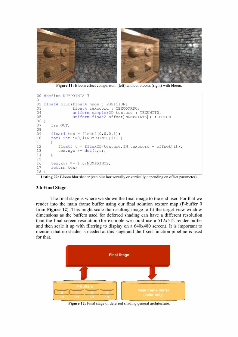
Figure 11: Bloom effect comparison: (left) without bloom, (right) with bloom.

00 #define NUMPOINTS 70102 float4 blur(float4 hpos : POSITION;03 float4 texcoord : TEXCOORD0;04 uniform sampler2D texture : TEXUNIT0,05 uniform float2 offset[NUMPOINTS]) : COLOR06 {07 f2s OUT;0809 float4 tex = float4(0,0,0,1);10 for( int i=0;i<NUMPOINTS;i++ )11 {12 float3 t = f3tex2D(texture,IN.texcoord + offset[i]);13 tex.xyz += dot(t,t);14 }1516 tex.xyz *= 1.0/NUMPOINTS;17 return tex;18 }

Listing 22: Bloom blur shader (can blur horizontally or vertically depending on offset parameter).

3.6 Final Stage

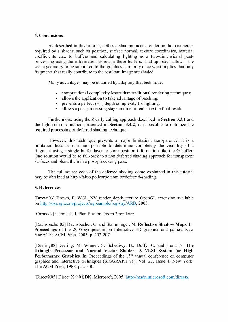
The final stage is where we shown the final image to the end user. For that we render into the main frame buffer using our final solution texture map (P-buffer 0 from Figure 12). This might scale the resulting image to fit the target view window dimensions as the buffers used for deferred shading can have a different resolution than the final screen resolution (for example we could use a 512x512 render buffer and then scale it up with filtering to display on a 640x480 screen). It is important to mention that no shader is needed at this stage and the fixed function pipeline is used for that.

Final Stage

Main frame buffer(color only)

P-buffers

10 2 3full full 1/4 1/4

Final Stage


P-buffers

10 2 3full full 1/4 1/4




P-buffers

10 2 3full full 1/4 1/4

P-buffers

10 2 3full full 1/4 1/4

P-buffers

1100 22 33full full 1/4 1/4

Figure 12: Final stage of deferred shading general architecture.

4. Conclusions

As described in this tutorial, deferred shading means rendering the parameters required by a shader, such as position, surface normal, texture coordinates, material coefficients etc., to buffers and calculating lighting as a two-dimensional post-processing using the information stored in these buffers. That approach allows the scene geometry to be submitted to the graphics card only once what implies that only fragments that really contribute to the resultant image are shaded.

Many advantages may be obtained by adopting that technique:

• computational complexity lesser than traditional rendering techniques;• allows the application to take advantage of batching;• presents a perfect O(1) depth complexity for lighting;• allows a post-processing stage in order to enhance the final result.

Furthermore, using the Z early culling approach described in Section 3.3.1 and the light scissors method presented in Section 3.4.2, it is possible to optimize the required processing of deferred shading technique.

However, this technique presents a major limitation: transparency. It is a limitation because it is not possible to determine completely the visibility of a fragment using a single buffer layer to store position information like the G-buffer. One solution would be to fall-back to a non deferred shading approach for transparent surfaces and blend them in a post-processing pass.

The full source code of the deferred shading demo explained in this tutorial may be obtained at http://fabio.policarpo.nom.br/deferred-shading.

5. References

[Brown03] Brown, P. WGL_NV_render_depth_texture OpenGL extension available on http://oss.sgi.com/projects/ogl-sample/registry/ARB, 2003.

[Carmack] Carmack, J. Plan files on Doom 3 renderer.

[Dachsbacher05] Dachsbacher, C. and Stamminger, M. Reflective Shadow Maps. In: Proceedings of the 2005 symposium on Interactive 3D graphics and games. New York: The ACM Press, 2005. p. 203-207.

[Deering88] Deering, M; Winner, S; Schediwy, B.; Duffy, C. and Hunt, N. The Triangle Processor and Normal Vector Shader: A VLSI System for High Performance Graphics. In: Proceedings of the 15th annual conference on computer graphics and interactive techniques (SIGGRAPH 88). Vol. 22, Issue 4. New York: The ACM Press, 1988. p. 21-30.

[DirectX05] Direct X 9.0 SDK, Microsoft, 2005. http://msdn.microsoft.com/directx

http://oss.sgi.com/projects/ogl-sample/registry/ARB

http://msdn.microsoft.com/directx

[Ellsworth91] Ellsworth, D. E. Parallel Architectures and Algorithms for Real-time Synthesis of High-quality Images using Deferred Shading. In: Workshop on Algorithms and Parallel VLSI Architectures. Pont-a-Mousson, France, June 12, 1991.

[Eyles97] Eyles, J.; Molnar, S.; Poulton, J.; Greer, T.; Lastra, A.; England, N. and Westover, Lee. PixelFlow: The Realization. In: Proceedings of the ACM SIGGRAPH / EUROGRAPHICS workshop on Graphics Hardware. New York: The ACM Press, 1997. p. 57-68.

[Fernando03] Fernando, R. and Kilgard, M. The Cg Tutorial: The Definitive Guide to Programmable Real-Time Graphics. Addison-Wesley. NVidia, 2003. p. 384.

[Gouraud71] Gouraud, H. Continuous shading of curved surfaces. IEEE Transactions on Computers. Vol. C-20. 1971. p. 623-629.

[Kirkland02] Kirkland, D.; Poddar, B. and Urquhart, S. WGL_ARB_pbuffer OpenGL extension available on http://oss.sgi.com/projects/ogl-sample/registry/ARB, 2002.

[Kontkanen05] Kontkanen, J. and Laine, S. Ambient Occlusion Fields. In: Proceedings of the 2005 symposium on Interactive 3D graphics and games. New York: The ACM Press, 2005. p. 41-48.

[Lastra95] Lastra, A.; Molnar, S.; Olano, M. and Wang, Y. Real-Time Programmable Shading. In: Proceedings of the 1995 Symposium on Interactive 3D graphics. New York: The ACM Press, 1995. p. 59-66.

[Lengyel03] Lengyel, E. Mathematics for 3D Game Programming and Computer Graphics. 2nd edition. Delmar Thomson Learning, 2003. p. 551.

[Mace02] Mace, R. GL_ATI_draw_buffers OpenGL extension available on http://oss.sgi.com/projects/ogl-sample/registry/ARB, 2002.

[Möller02] Akenine-Möller, T. and Haines, E. Real-Time Rendering. 2nd edition. A K Peters, 2002. p. 835.

[Molnar92] Molnar, S.; Eyles, J. and Poulton, J. PixelFlow: high-speed rendering using image composition. In: Proceedings of the 19th annual conference on computer graphics and interactive techniques (SIGGRAPH 92). Vol. 26, Issue 2. New York: The ACM Press, 1992. p. 231-240.

[Nicodemus77] Nicodemus, F. E.; Richmond, J. C.; Hsia, J. J.; Ginsberg, I. W. and Limperis, T. Geometric Considerations and Nomenclature for Reflectance. National Bureau of Standards (US), October 1977.

[Olano97] Olano, M. and Greer, T. Triangle Scan Conversion using 2D Homogeneous Coordinates. In: Proceedings of the ACM SIGGRAPH / EUROGRAPHICS workshop on Graphics Hardware. New York: The ACM Press, 1997. p. 89-95.



[Olano98] Olano, M. and Lastra, A. A Shading Language on Graphics Hardware: The PixelFlow Shading System. In: Proceedings of the 25th annual conference on computer graphics and interactive techniques (SIGGRAPH 98). New York: The ACM Press, 1998. p. 159-168.

[Pharr05] Pharr, M. and Fernando, R. GPU Gems 2: Programming Techniques for High-Performance Graphics and General-Purpose Computation. Addison-Wesley. NVidia, 2005. p. 880.

[Phong75] Phong, B. T. Illumination for Computer Generated Pictures. Communications of the ACM. Vol. 18, No. 6. 1975. p. 311-317.

[Poddar01] Poddar, B. and Womack, P. WGL_ARB_render_texture OpenGL extension available on http://oss.sgi.com/projects/ogl-sample/registry/ARB, 2001.

[Policarpo05] Policarpo, F.; Lopes, G. and Fonseca F. P3D Render Library. http://www.fabio.policarpo.nom.br/p3d/index.htm, 2005.

[Rhoades92] Rhoades, J.; Turk, G.; Bell, A.; State, A.; Neumann, U. and Varshney, A. Real-time procedural textures. In: Proceedings of the 1992 Symposium on Interactive 3D graphics. New York: The ACM Press, 1992. p. 95-100.

[Saito90] Saito, T. and Takahashi, T. Comprehensible rendering of 3-D shapes. In: Proceedings of the 17th annual conference on computer graphics and interactive techniques (SIGGRAPH 90). Vol. 24, Issue 4. New York: The ACM Press, 1990. p. 197-206.

[Shreiner03] Shreiner, D.; Woo, M.; Neider, J. and Davis, T. OpenGL Programming Guide: The Official Guide to Learning OpenGL, Version 1.4. Addison-Wesley, 2003. p. 800.

[Stroustrup97] Stroustrup, B. The C++ Programming Language. 3rd edition. Addison-Wesley, 1997. p. 911.

[Zwicker01] Zwicker, M.; Pfister, H.; Baar, J. and Gross, M. Surface Splatting. In: Proceedings of the 28th annual conference on computer graphics and interactive techniques (SIGGRAPH 01). New York: The ACM Press, 2001. p. 371-378.

6. Appendix A

Below, all steps from the complete deferred shading pipeline are shown.

1. Geometry stage (3D) - render depth pass to G-buffer depth buffer (no shader needed) - render geometry with materials to G-buffer color, aux0 and aux1 buffers (normal, diffuse and specular)2. Ligthing stage (2D) - render ambient pass into P-buffer 0 using diffuse G-buffer texture modulated by ambient color (no shader needed) - render lighting passes with additive blending into P-buffer 03. Post-processing stage (2D) - if bloom enabled

http://www.fabio.policarpo.nom.br/p3d/index.htm


- render bloom horizontal blur into P-buffer 2 using P-buffer 0 as texture - render bloom vertical blur into P-buffer 3 using P-buffer 2 as texture - add final bloom texture to P-buffer 0 using P-buffer 3 as texture (no shader needed) - if anti-aliasing enabled - render anti-aliasing into P-buffer 1 using P-buffer 0 as texture - swap P-buffer 0 and 1 so that P-buffer 0 holds final image4. Final stage (2D) - render final image into main frame buffer using P-buffer 0 as texture (no shader needed)

Documents

Deferred Shading Tutorial