1

Decrease axial vibration generator with balancing

Guillaume Christin1, Nicolas Péton

2

1GE Measurement & Control, 68 chemin des Ormeaux, 69760 Limonest, France

2GE Measurement & Control, 14 rue de la Haltinière, 44303 Nantes, France

Abstract GE’s Machinery Diagnostic Services team was invited to investigate vibration issue on generator installed on

a power plant. Machine train consists of a generator and a gas turbine. The unit was under commissioning

since 2 years and there was not any vibration issue until axial vibration was measured with a temporary

accelerometer at NDE generator bearing. The axial vibrations at the bearing location were not monitored for

this machine. Vibration testing was carried out using ADRE 408 DSPi (Dynamic Signal Processing

Instrument) to hook up vibration data from the existing Bently Nevada’s 3500 Series vibration monitor

system. Relative vibration data were collected from the Bently Nevada’s Rack 3500 monitor buffered

outputs. Each of the Machine Train’s bearings is monitored by Bently Nevada XY proximity probe pair and

one vertical absolute velocity transducer fixed on the bearing housing. Absolute vibration data were collected

from the velocity transducer buffered outputs in the Mark VI cabinet. Moreover, a temporary axial

accelerometer was installed on the NDE generator bearing housing. The shaft rotates counter clockwise,

when viewed from the driver (Gas Turbine) to the driven (Generator).

A periodic vibration measurement, on a route based monitoring schedule, allowed the customer to observe an

increasing trend of casing vibration in the radial and axial directions on both of generator bearings. There

was a significant increase in vibration amplitudes in the axial direction of generator NDE bearing in

situations similar to a full load conditions (i.e. base load of 75 MW) during the months of July, August and

September. A first axial vibration analysis was carried out in order to characterize the phenomenon. An axial

structural resonance of the NDE generator bearing housing was highlighted. An inspection of the NDE

generator bearing support and pedestal inspection was done. Everything was correct and respects the

specifications. From experience, the fact to balance a unit with radial vibration measurement can decrease

the axial vibration because of the cross effect between radial and axial dynamic stiffness. The generator

disposed of two balancing planes. First, the balance trim was carried out following the method of the

influence vectors. In order to optimize the balancing and since the vibration were mainly out of phase

between both bearings, the influence vector method was linked to the couple-static method. The axial

vibrations were decreased by more than 60%

1 Discusion

1.1 Machine train

Machine train as shown in Fig. 1 consists of a gas turbine driven a Generator via a gear. Each of the

machine train’s bearing is monitored by one vertical seismic probe and displacement transducers mounted on

the machine casing in a plane (XY) perpendicular to the rotor axis of the machine to observe radial motion of

the shaft. The XY pairs of non-contacting proximity probes are mounted at 45-degrees left (Y-probe) and 45-

degree right (X-probe). One axial seismic probe was temporary mounted on NDE generator bearing support.

The machine train diagram is shown in Fig 1. The shaft rotates counter clockwise, when viewed from the

driver to the driven.

2

Figure 1: Machine train layout

1.2 Description of the issue

The unit had been under commissioning for 2 years and there was no vibration issue until axial vibration

was measured with a temporary accelerometer at NDE generator bearing. The axial vibration at bearing

location was not monitored for this machine. There is no limitation and obligation in any of the international

standard to take care of the axial vibration.

A periodic vibration measurement was carried out by the customer to monitor the casing vibration in

radial and axial directions on both of generator bearings. There was significant increase in vibration

amplitude in axial direction of generator NDE bearing in similar load conditions i.e. base load i.e. 75 MW in

the months of July, August and September. The level of axial vibration reached around 0.4 in/s rms. An

inspection of the NDE generator bearing support and pedestal inspection was done. Everything was correct

and as per the specifications. Consequently, it was decided to carry on a first axial vibration analyzed to

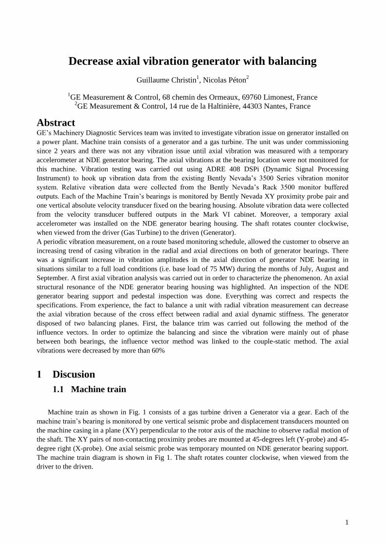
characterize the axial vibration behavior on the NDE generator bearing support. The machine was run at full

speed and steady state condition. An axial accelerometer was fitted with magnetic support at different

locations (See Fig2) on the NDE generator bearing support while the machine was running at identical

condition. From this test, an axial structural resonance of the NDE generator bearing housing was

highlighted. The fact that the vibration level was decreasing from 12 mm/s rms to 2 mm/s rms by reduction

of only 300 rpm, confirmed the presence of a resonance in axial direction

Axial (on bearing support)

NDE generator bearing

3

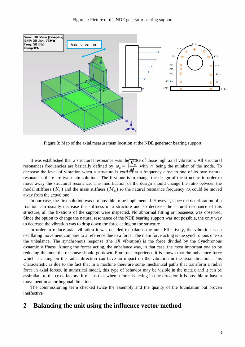
Figure 2: Picture of the NDE generator bearing support

Figure 3: Map of the axial measurement location at the NDE generator bearing support

It was established that a structural resonance was the cause of those high axial vibration. All structural

resonances frequencies are basically defined by n

nn

M

K .with n being the number of the mode. To

decrease the level of vibration when a structure is excited at a frequency close to one of its own natural

resonances there are two main solutions. The first one is to change the design of the structure in order to

move away the structural resonance. The modification of the design should change the ratio between the

modal stiffness ( nK ) and the mass stiffness ( nM ) so the natural resonance frequency n could be moved

away from the actual one

In our case, the first solution was not possible to be implemented. However, since the deterioration of a

fixation can usually decrease the stiffness of a structure and so decrease the natural resonance of this

structure, all the fixations of the support were inspected. No abnormal fitting or looseness was observed.

Since the option to change the natural resonance of the NDE bearing support was not possible, the only way

to decrease the vibration was to drop down the force acting on the structure

In order to reduce axial vibration it was decided to balance the unit. Effectively, the vibration is an

oscillating movement compare to a reference due to a force. The main force acting is the synchronous one so

the unbalance. The synchronous response (the 1X vibration) is the force divided by the Synchronous

dynamic stiffness. Among the forces acting, the unbalance was, in that case, the most important one so by

reducing this one, the response should go down. From our experience it is known that the unbalance force

which is acting on the radial direction can have an impact on the vibration in the axial direction. This

characteristic is due to the fact that in a machine there are some mechanical paths that transform a radial

force in axial forces. In numerical model, this type of behavior may be visible in the matrix and it can be

assimilate to the cross-factors. It means that when a force is acting in one direction it is possible to have a

movement in an orthogonal direction

The commissioning team checked twice the assembly and the quality of the foundation but proven

ineffective

2 Balancing the unit using the influence vector method

Axial vibration

4

The vibration signal was mainly due to synchronous component (1X) and the 1X component was

increasing with the speed. The behaviour of the machine was the same during start up and shutdown which

means that the behaviour of this phenomenon was repeatable. The behaviour of the machine seemed to be

repeatable between a startup and the shutdown associated. It was observed that the orbit shape was elliptical

with a forward precession. Since the unbalance is a forward force the fact to reduce this force should

decrease the forward vibration. From all the previous observations, it was decided to try to balance the unit

Selecting a trial weight can be a dangerous proposition. In many cases, the vibration on the machine is

already high, and adding an excessive trial weight could increase the vibration amplitudes. So a good

practice is to at least get a correct trial weight location to be opposite at the actual residual unbalance location

and add enough weight to get some response. This selection is not easy unless a reasonable amount of

information is known about the machine. Adequate trial weight would be considered to be enough weight to

produce a 10% change in vibration vector based on the original vibration

Before presenting the trim balance of this unit, it is important to review the influence vectors method.

Basically, this method consists in installing a trial weight in a balance plane and in observing what is the

influence of this mass on all the vibration response. This action has to be repeated for all the balance planes

available on the machine. Then software like Bently Balance will propose an optimal solution to install one

correction weight in one location for each balance plane

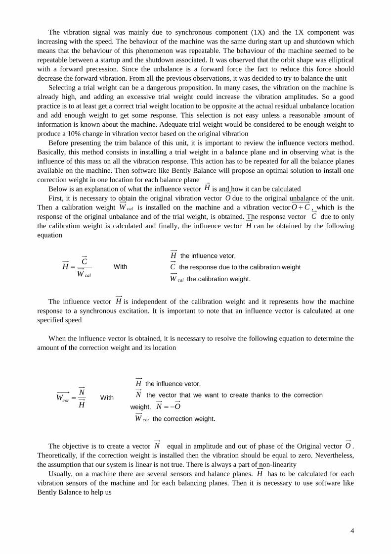
Below is an explanation of what the influence vector H

is and how it can be calculated

First, it is necessary to obtain the original vibration vector O due to the original unbalance of the unit.

Then a calibration weight calW is installed on the machine and a vibration vector CO , which is the

response of the original unbalance and of the trial weight, is obtained. The response vector C due to only

the calibration weight is calculated and finally, the influence vector H can be obtained by the following

equation

calW

CH With

The influence vector H is independent of the calibration weight and it represents how the machine

response to a synchronous excitation. It is important to note that an influence vector is calculated at one

specified speed

When the influence vector is obtained, it is necessary to resolve the following equation to determine the

amount of the correction weight and its location

H

NWcor With

The objective is to create a vector N equal in amplitude and out of phase of the Original vector O .

Theoretically, if the correction weight is installed then the vibration should be equal to zero. Nevertheless,

the assumption that our system is linear is not true. There is always a part of non-linearity

Usually, on a machine there are several sensors and balance planes. H has to be calculated for each

vibration sensors of the machine and for each balancing planes. Then it is necessary to use software like

Bently Balance to help us

H the influence vetor,

C the response due to the calibration weight

calW the calibration weight.

H the influence vetor,

N the vector that we want to create thanks to the correction

weight. ON

corW the correction weight.

5

When a trim balance is carrying out with the support of a software like Bently Balance, the number of

influence vector ( ijH ) is equal to ji with i the number of sensors and j the number of balancing planes.

In this case, the following system has to be solved

0 jiji WcorHO

The above equation is an over determined systems of linear equations since there are more equations than

variables. In order to solve this equation system, the software uses a least mean square method to decrease

the level of vibration for all the sensors. Effectively there is not one perfect solution to solve this system

The trim balance of this generator unit was done using this influence vector methodology and Bently

Balance software

A first run, named the REF RUN, was done in order to get cold reference data (One start up (SU) and

one run at Full Speed No Load (FSNL) during 2-5 minutes and then a shutdown (SD)). Then another run

(RUN1) was done at Full Speed Full Load (FSFL) during 1 hours in order to check if any thermal

phenomenon had an influence on the vibration behavior. No influence was observed between FSFL and

FSNL

Since the vibration behaviour of the generator was similar between FSFL and FSNL it was decided to

balance the unit at FSNL. This method saved time and cost to balance the unit. The generator was balanced

using the influence vector method

Two balance planes were available on the generator. It is important to remember that even if there are

two or more planes available it is not necessary to use all of them. The more the number of used balance

plane is important the more the price of the trim balance will be expensive (time cost, gas cost, loss of

production…etc. ...). The fact to use one more balance plane is equivalent to do one more run. This need has

to be justified to the customer

In order to determine if two planes are needed, the first thing to do is to compare the phase relationship

between DE 1X vectors and NDE 1X vectors. Obviously, this comparison has to be done for probes which

are installed in the same angular position. The objective is to understand which lateral rotor mode dominates

the dynamic behaviour of the rotor

If a machine is mainly influenced by its first mode then the 1X vectors should be in phase. So, wherever

the weight is installed along the rotor (in opposite position of the heavy spot) the vibration should decrease.

This last sentence is true only if the second mode of the rotor is far from the operating speed and do not have

any influence at the operating speed

From our data, it appears that the generator was mainly influenced by its second mode since the 1X

vectors were out of phase from one bearing (DE) to another bearing (NDE). It was then decided to use both

balance planes

2.1 First trial run

A first trial weight of 392g was installed at 30° CCW from the keyphasor notch (when looking from the

generator to the turbine) on the balance plane at NDE generator side. and the machine was run to FSNL

during 2 minutes

6

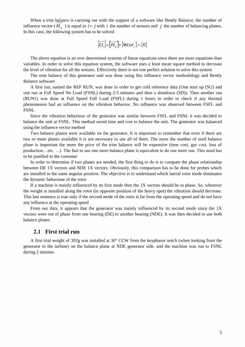
Figure 4: Details of the bearing #8 balance plane and picture of the installed trial weights

The polar plots (Fig 5 & Fig 6) show that the weight had an influence on the vibration since the 1X

amplitude and the 1X angle changed for all the probes. The vibration units (in/s pk) are from the American

system. Since the goal of this balance activity was to reduce the (axial) seismic vibration at NDE end, the

plots of the velocity probes will be presented in this article

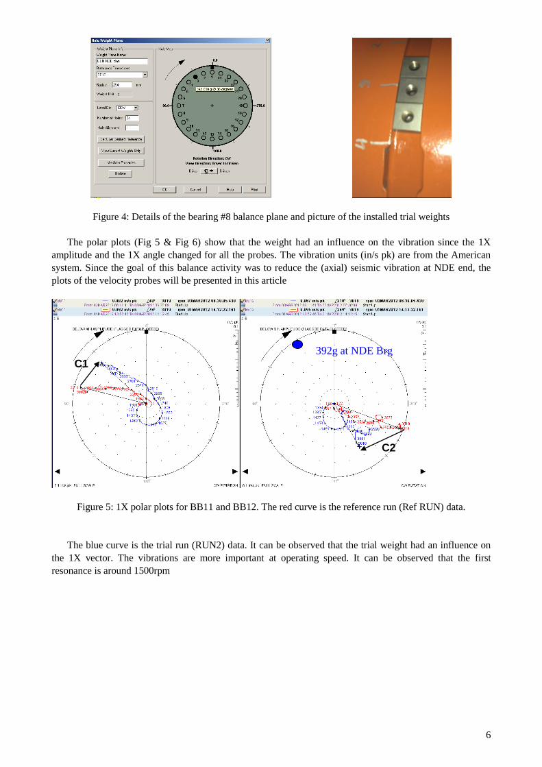
Figure 5: 1X polar plots for BB11 and BB12. The red curve is the reference run (Ref RUN) data.

The blue curve is the trial run (RUN2) data. It can be observed that the trial weight had an influence on

the 1X vector. The vibrations are more important at operating speed. It can be observed that the first

resonance is around 1500rpm

C1

C2

392g at NDE Brg

7

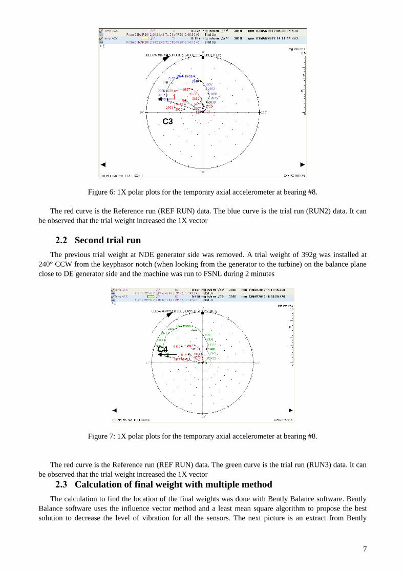
Figure 6: 1X polar plots for the temporary axial accelerometer at bearing #8.

The red curve is the Reference run (REF RUN) data. The blue curve is the trial run (RUN2) data. It can

be observed that the trial weight increased the 1X vector

2.2 Second trial run

The previous trial weight at NDE generator side was removed. A trial weight of 392g was installed at

240° CCW from the keyphasor notch (when looking from the generator to the turbine) on the balance plane

close to DE generator side and the machine was run to FSNL during 2 minutes

Figure 7: 1X polar plots for the temporary axial accelerometer at bearing #8.

The red curve is the Reference run (REF RUN) data. The green curve is the trial run (RUN3) data. It can

be observed that the trial weight increased the 1X vector

2.3 Calculation of final weight with multiple method

The calculation to find the location of the final weights was done with Bently Balance software. Bently

Balance software uses the influence vector method and a least mean square algorithm to propose the best

solution to decrease the level of vibration for all the sensors. The next picture is an extract from Bently

C3

C4

8

Balance software. In the green area, Bently Balance advices to add one mass of 899g@322° in NDE GEN

plane and another mass of 205g@252° in DE GEN plane. In the blue area, predicted results of the final

vibration are shown if the proposed solution is applied. In the orange area, the original vibration vectors are

shown

Figure 8: Results extracted from Bently Balance software. Multi plane method results.

The solution proposed by the software was not possible to implement since the weight was too heavy.

The maximum weight available was around 330g. The algorithm used in Bently Balance doesn’t have any

weight limitation. It proposes a solution to obtain the best result

The next step could be to use BentlyBalance and simulate several solutions. A first solution that could be

tested is to replace the maximum solution weight (840g) by the maximum available weight (330g). The value

of the second weight (205g) was changed to 75g (205x330/899) in order to keep the proportionality with the

first solution. The next table shows that the predicted results are not really good compare to the original

solution

Figure 9: Results extracted from Bently Balance software. Alternative calculation.

9

Infinity of other solutions could be tested but it is not really scientific. So it was decided to associate the

influence vector method and the Static-Couple method in order to guide us to the best final solution

3 Optimise the trim balance with Static/Couple method

3.1 Static/Couple method review

Let’s review first the static-couple method. In this method, vectors at two planes are decomposed into in-

phase (static) and out-of-phase (couple) components. The static component can be due to the first mode or

third mode. The couple component is typically due to the second mode. Static weight is defined as the

weights placed at two ends with the same orientation (in-phase), whereas couple weight is defined as the

weights placed at two ends with the opposite orientation (out-of-phase)

.

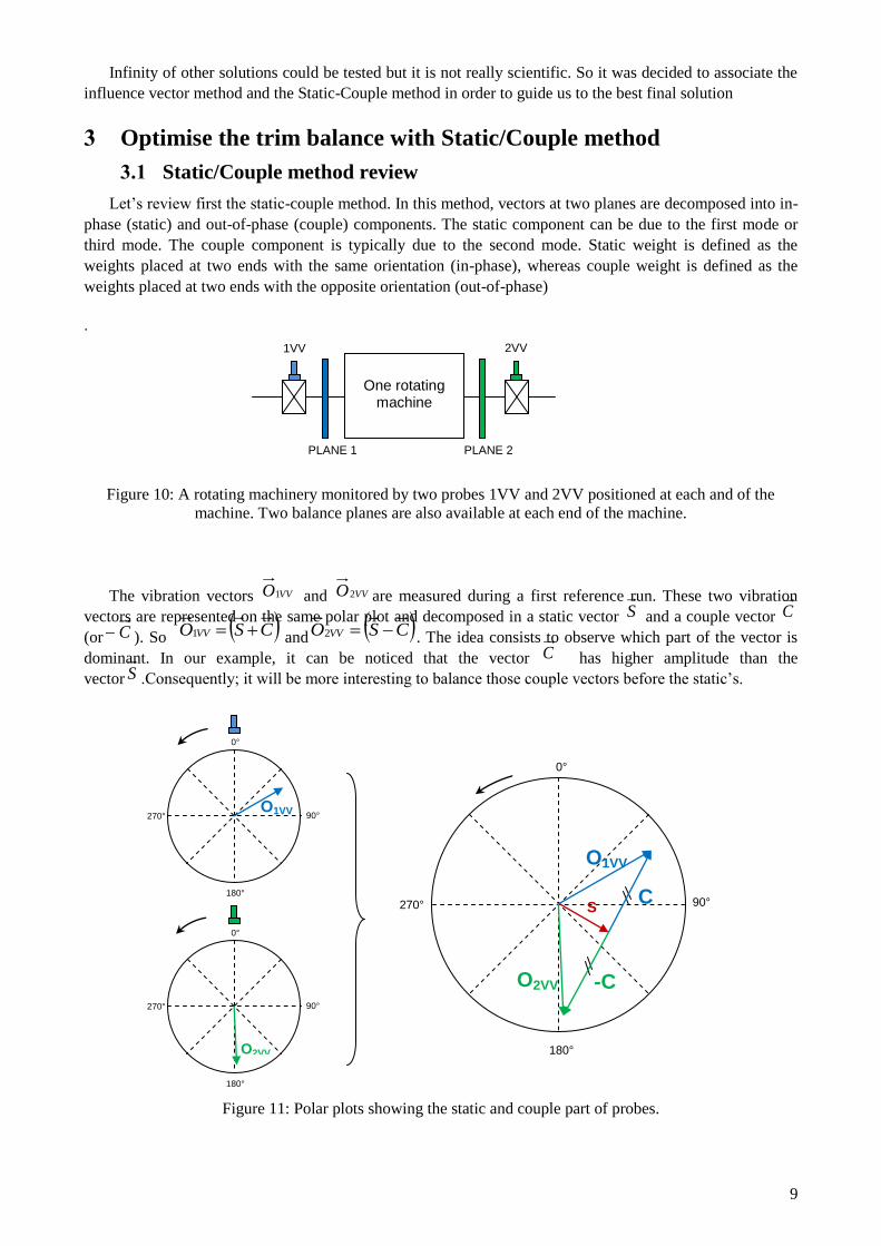
Figure 10: A rotating machinery monitored by two probes 1VV and 2VV positioned at each and of the

machine. Two balance planes are also available at each end of the machine.

The vibration vectors VVO1 and VVO2 are measured during a first reference run. These two vibration

vectors are represented on the same polar plot and decomposed in a static vector S and a couple vector C

(or C ). So CSO VV 1 and CSO VV 2 . The idea consists to observe which part of the vector is

dominant. In our example, it can be noticed that the vector C has higher amplitude than the

vector S .Consequently; it will be more interesting to balance those couple vectors before the static’s.

Figure 11: Polar plots showing the static and couple part of probes.

One rotating

machine

2VV 1VV

PLANE 1 PLANE 2

0°

90°

180°

270° O1VV

0°

90°

180°

270°

O2VV

O1VV

O2VV

C

-C

S

0°

90° 270°

180°

10

The trial weights should be installed in opposition of phase in each plane as illustrated in the following

picture. The new vibrations vectors should be measured and the influence vectors calculated for both sensors

To balance the static vector, two trial weights have to be installed at the same angular orientation in each

plan. The new vibration vectors should be measured and the influence vectors calculated for both sensors

This method can be really efficient on symmetrical machine like generator and allows balancing

separately the first mode and the second mode. The influence vector obtained for this example are

named SSH , SCH CSH and CCH .

Then, the following system has to be solved to determine Ws (the static weight) and Wc (the couple weight).

0

0

Wc

Ws

HH

scHH

C

S

CCCS

SS

The influence vectors obtained for the static-couple method are different from the influence vectors use

with the multi plane method. However, it is proven that the influence vectors of one method can be used to

calculate the influence vectors of the other method

Sometimes for an asymmetric rotor, or due to influence via couplings from adjacent rotors, the first/third

mode shape (in-phase) may not be very symmetric and the second mode shape (out-of-phase) may not be

very anti-symmetric. In this case, cross-effects may need to be included

If both direct and cross-effect influence coefficients are included, then theoretically the rotor can be

balanced perfectly. The new format of influence data for the static-couple model is comparable to that for the

multi-plane balance model

Sometimes one needs to know individual probe influence due to static or couple weights only. The static

weight influence to probes near planes 1 and 2 can be given by h1,S and h2,S , while the couple weight

influence to probes near planes 1 and 2 can be given by h1,C and h2,C

Conversion equations can be developed to obtain direct and cross-effect static-couple influence

coefficients from the four influence coefficients of the multi-plane balance model or to obtain the four

influence coefficients of the multi-plane balance model from direct and cross-effect static-couple influence

coefficients

Concerning our historical case, direct and cross-effect static-couple influence coefficients were

calculated from the four influence coefficients of the multi-plane balance model. The next formula developed

in the literature [1] was used

21122211

2

1hhhhH SS

90°

180°

0°

270°

0°

270°

180°

90°

PLAN 1

TRIAL Weights locations (out of phase)

to balance Couple part

TRIAL Weights locations (In phase)

to balance Static part

90°

180°

0°

270° 90°

11

21122211

2

1hhhhH CS

21122211

2

1hhhhH SC

21122211

2

1hhhhH CC

3.2 Balance the generator using both method static/couple and multi plane

A complete excel file was developed to easily obtained the Static-Couple influence vector from the

multi-plane influence vector method. Using this tools all the static-couple influence vectors were obtained

for the generator

In order to details the procedure, the example for proximity probes 39VS91, 39VS92, 39VS101 and

39VS102 will be presented. First it is necessary to come back to the values of the original vectors

DE Plane NDE Plane

O vectors O vectors

39VS91 45°R 0.38@137° 39VS101 45°R 0.309@306°

39VS92 45°L 2.25@23° 39VS102 45°L 1.298@192°

Then, in order to eliminate the effect of the anisotropic stiffness, the forward and reverse component for

both pair of probes 39VS91/92 and 39VS101 /102 were calculated

DE Plane NDE Plane 39VS91/92 39VS101/102

Forward

1.30@116° Forward 0.79@287°

Reverse

0.95@288°

Reverse 0.51@95°

It can be observed that the reverse component was not negligible compare to the forward component.

Then the static and couple components were calculated for this pair of 1X forward vector

Static 0.27@129° Couple 1.04@113°

The couple component is much more import than the static. So it was decided to balance only the couple

component. To do it, it is necessary to have the CCH influence vector and the original couple part vector

that was calculated above (1.04@113°).

After using the previous equation, the following Static-Couple influence vectors matrix was obtained

7@1120,003135885@1390,00034782

1@1750,000179059@330,00042923

CCCS

SS

HH

scHHmil pp /g

The influence vector for the couple part CCH is equal to 7@1120,00313588 . The next equation has to

be solved to obtain the amount and the locations of the couple weights to balance the unit

CC

corH

NWc With

CCH the influence vector of the couple component,

N the vector that we want to create thanks to the correction

weight. CN (with C the couple component).

corcW the Couple correction weight.

12

Finally, this calculation proposed a solution of 331g@0° on NDE generator and 331°@180° on DE

generator. The amount of weight proposed by this solution was possible to implement on the generator.

Before to implement this solution, this result was tested in Bently Balance to check the predicted results

Figure 12: Results extracted from Bently Balance software. Alternative calculation for static/couple method.

In the blue area, it can see that this alternative solution works but could be better. Several other

alternative simulations were tested in Bently Balance close to this one. The best and final results were

obtained for one weight of 331g@330°CCW at NDE generator and one weight of 331g@150°CCW at

DE generator. The fact to shift the solution of 30° increases a lot the predictive results (see next table)

Figure 13: Results extracted from Bently Balance software. Alternative calculation for final solution

obtained with the combination of multi plan method and the static couple method.

3.3 Final run with solution from static/couple method & multiplane

method

13

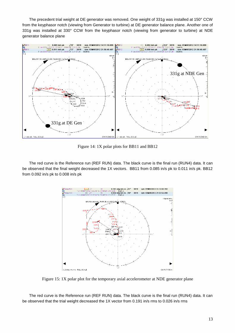
The precedent trial weight at DE generator was removed. One weight of 331g was installed at 150° CCW

from the keyphasor notch (viewing from Generator to turbine) at DE generator balance plane. Another one of

331g was installed at 330° CCW from the keyphasor notch (viewing from generator to turbine) at NDE

generator balance plane

Figure 14: 1X polar plots for BB11 and BB12

The red curve is the Reference run (REF RUN) data. The black curve is the final run (RUN4) data. It can

be observed that the final weight decreased the 1X vectors. BB11 from 0.085 in/s pk to 0.011 in/s pk. BB12

from 0.092 in/s pk to 0.008 in/s pk

Figure 15: 1X polar plot for the temporary axial accelerometer at NDE generator plane

The red curve is the Reference run (REF RUN) data. The black curve is the final run (RUN4) data. It can

be observed that the trial weight decreased the 1X vector from 0.191 in/s rms to 0.026 in/s rms

331g at DE Gen

331g at NDE Gen

14

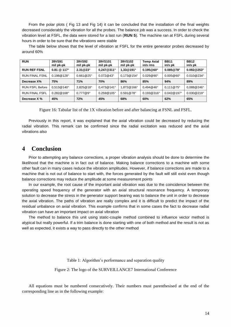
From the polar plots ( Fig 13 and Fig 14) it can be concluded that the installation of the final weights

decreased considerably the vibration for all the probes. The balance job was a success. In order to check the

vibration level at FSFL, the data were stored for a last run (RUN 5). The machine ran at FSFL during several

hours in order to be sure that the vibrations were stable

The table below shows that the level of vibration at FSFL for the entire generator probes decreased by

around 60%

RUN 39VS91

mil pk-pk 39VS92 mil pk-pk

39VS101 mil pk-pk

39VS102 mil pk-pk

Temp Axial in/s rms

BB11 in/s pk

BB12 in/s pk

RUN REF FSNL 0.81 @ 117° 2.31@23° 0,247@311° 1,33@191° 0.195@60° 0.085@78° 0.092@253°

RUN FINAL FSNL 0.198@128° 0.661@25° 0.072@43° 0,173@154° 0.029@90° 0.005@60° 0.010@234°

Decrease X% 75% 71% 70% 86% 85% 94% 89%

RUN FSFL Before 0,513@140° 2,825@18° 0,473@141° 1,872@166° 0,494@46° 0,111@75° 0,088@246°

RUN FINAL FSFL 0.282@168° 0.777@9° 0.259@105° 0.591@78° 0.193@316° 0.042@197° 0.030@219°

Decrease X % 45% 72% 45% 68% 60% 62% 65%

Figure 16: Tabular list of the 1X vibration before and after balancing at FSNL and FSFL.

Previously in this report, it was explained that the axial vibration could be decreased by reducing the

radial vibration. This remark can be confirmed since the radial excitation was reduced and the axial

vibrations also

4 Conclusion

Prior to attempting any balance corrections, a proper vibration analysis should be done to determine the

likelihood that the machine is in fact out of balance. Making balance corrections to a machine with some

other fault can in many cases reduce the vibration amplitudes. However, if balance corrections are made to a

machine that is not out of balance to start with, the forces generated by the fault will still exist even though

balance corrections may reduce the amplitude at some measurement points

In our example, the root cause of the important axial vibration was due to the coincidence between the

operating speed frequency of the generator with an axial structural resonance frequency. A temporary

solution to decrease the stress in the generator support bearing was to balance the unit in order to decrease

the axial vibration. The paths of vibration are really complex and it is difficult to predict the impact of the

residual unbalance on axial vibration. This example confirms that in some cases the fact to decrease radial

vibration can have an important impact on axial vibration

The method to balance this unit using static-couple method combined to influence vector method is

atypical but really powerful. If a trim balance is done starting with one of both method and the result is not as

well as expected, it exists a way to pass directly to the other method

Table 1: Algorithm’s performance and separation quality

Figure 2: The logo of the SURVEILLANCE7 International Conference

All equations must be numbered consecutively. Their numbers must parenthesised at the end of the

corresponding line as in the following example:

15

nAx (1)

References

[1] John J Yu. (2009) Relationship of influence coefficients between Static-Couple and Multiplane Methods

on two plane balancing. Volume 29 N°1 ORBIT.

[2] Donald E.Bently with Charles T.Hatch. Fundamentals of Rotating Machinery Diagnostics Edited by Bob

Grissom.