Deconstructing a Real Option Problem

8/2/2019 Deconstructing a Real Option Problem

http://slidepdf.com/reader/full/deconstructing-a-real-option-problem 1/5

Deconstructing a Real Option Problem by Shane A. Van Dalsem, PhD

What does Real Option mean? (from Investopedia.com)

An alternative or choice that becomes available with a business investment opportunity.

Note that this kind of option is not a derivative instrument, but an actual option (in the sense of "choice") that a business may gain by undertaking certain endeavors. For

example, by investing in a particular project, a company may have the real option

of expanding, downsizing, or abandoning other projects in the future. Other examples of

real options may be opportunities for R&D, M&A, and licensing.

They are referred to as "real" because they usually pertain to tangible assets, such as

capital equipment, rather than financial instruments. Taking into account real options can

greatly affect the valuation of potential investments. Oftentimes, however, valuation

methods, such as NPV, do not include the benefits that real options provide.

How do we value real options?

There are three general methods used to value real options: 1. discounted cash flows, 2. use of

the Black-Scholes option pricing model, and 3. financial engineering. In this tutorial, we’ll focus

on the first two methods.

The Problem

Toto Motors has developed a car that can run on natural gas and has patented the new type of

engine. If Toto begins manufacturing the car today, there is 30% chance that gas prices will

increase significantly and the demand for the car will be high, 50% chance that gas prices will

remain stable and demand for the car will be medium, and a 20% change that gas prices willdrop, and demand for the car will be low. These scenarios are shown in the following table.

The NPV is the present value of future cash inflows less the initial investment. If the company

waits for one year, the cash flows will remain the same for each scenario, but the firm will be

able to gauge whether demand will by high, medium, or low. If the demand is low, the firm will

not invest in one year. The risk-free rate is 6% and the WACC for the firm is 15%.

(Dollars in Millions)

Demand Prob.

Initial

Investment

Net Cash Flow for

Each of the 5

Following YearsHigh 0.3 $20 $12.0

Medium 0.5 $20 $8.5

Low 0.2 $20 $2.0

The above example is known as an investment timing option, because it gives the firm the ability

to wait to see what the demand will be like after some uncertainty is removed.



Discounted Cash Flow Method

The discounted cash flow method estimates the value of the option by determining the

expected increase in the present value of future cash flows by taking the option. In this case,

we’ll determine the NPV of the project if the project is taken today and the NPV of the project if

the firm waits a year to decide whether to invest in the project.


Demand Prob.

Initial

Investment

Net Cash Flow for

Each of the 5

Following Years NPV Prob. x NPV

High 0.3 $20 $12.0 $20.23 $6.07

Medium 0.5 $20 $8.5 $8.49 $4.25

Low 0.2 $20 $2.0 ($13.30) ($2.66)

Expected NPV $7.66

The firm can wait and see what demand will be. This will move out the decision to invest for

one year. In this case, the patent that the firm has provides for this option, as another firm will

not be able to come in and easily duplicate the process. A timeline of the cash flows, under High

demand, is as follows.

($20) $12 $12 $12 $12 $12

It would be entirely inappropriate to discount all of these cash flows back at the WACC. Why?

Because the initial investment is not a risky cash flow. Either the firm will choose to invest or

will choose not to invest. As a result, we will discount the initial investment, to occur in one

year, back to the present using the risk free rate. The other cash flows are risky cash flows and

should be discounted back at the WACC. Using different discount rates for different cash flows

based on the riskiness of the individual cash flow is known as the certainty equivalent approach.

The following table represents the expected outcomes if the firm decides to wait a year to

invest.

0 1 2 3 4 5 6




Demand Prob.

Initial

Investment

Net Cash Flow for

Each of the 5

Following Years NPV Prob. x NPV

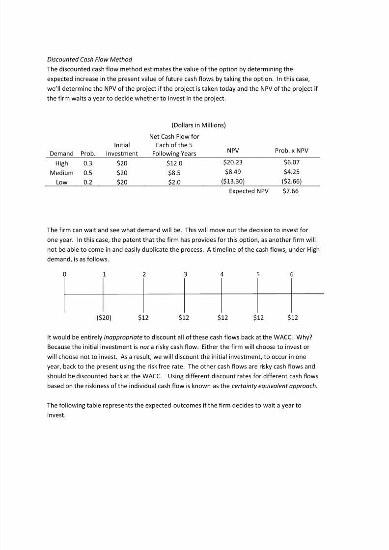
High 0.3 $20 $12.0 $16.11 $4.83

Medium 0.5 $20 $8.5 $5.91 $2.95

Low 0.2 $20 $2.0 Will not invest

Expected NPV $7.79

The firm will not invest if in one year, the demand for the car is low. The expected outcome

from making the decision to invest in a year is $7.79 million. The value of the option, using the

discounted cash flow method, is then $7.79 million less $7.66 million, or $0.13 million.

Black-Scholes Option Pricing Method

Another popular method used to determine the value of the real options is using the Black-

Scholes Option pricing model. The decision to delay is similar to a call option on a stock. That is,

if the value of project increases (if the demand in a year is High or Medium rather than Low),

then the firm will want to exercise the option to invest. The inputs for the Black-Scholes model

are as follows:

S=Present value of the project if undertaken in a year. We will calculate this value as $24.05.

X=Exercise price of the project. This is the initial investment into the project.For this project it is $20 million.r=Risk-free rate. In this case it would be the yield on the 1 year t-bill or 6%.

t=The time that the firm has until the option has to be exercised. In this case it is 1 year.

σ=Volatility of the underlying cash flows.We will calculate this based on the expected cash flows of the project as 0.4039.

To calculate the present value of the future expected cash flows of the project if the project

begins in one year. The trick here is that, much like a pricing a call option on a stock, is that we

estimate the present value even if the project is not undertaken. That is, we will include the PV

of the project even if the demand is low. Additionally, the initial investment is not included in

the PV calculation. Based on this, timelines to represent the cash flows to be discounted back at

the WACC are as follows.



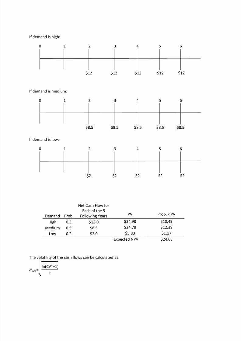
If demand is high:

$12 $12 $12 $12 $12

If demand is medium:

$8.5 $8.5 $8.5 $8.5 $8.5

If demand is low:

$2 $2 $2 $2 $2

Demand Prob.

Net Cash Flow for

Each of the 5

Following Years PV Prob. x PV

High 0.3 $12.0 $34.98 $10.49

Medium 0.5 $8.5 $24.78 $12.39

Low 0.2 $2.0 $5.83 $1.17

Expected NPV $24.05

The volatility of the cash flows can be calculated as:

= ln(CV2+1)

t

0 1 2 3 4 5 6

0 1 2 3 4 5 6

0 1 2 3 4 5 6



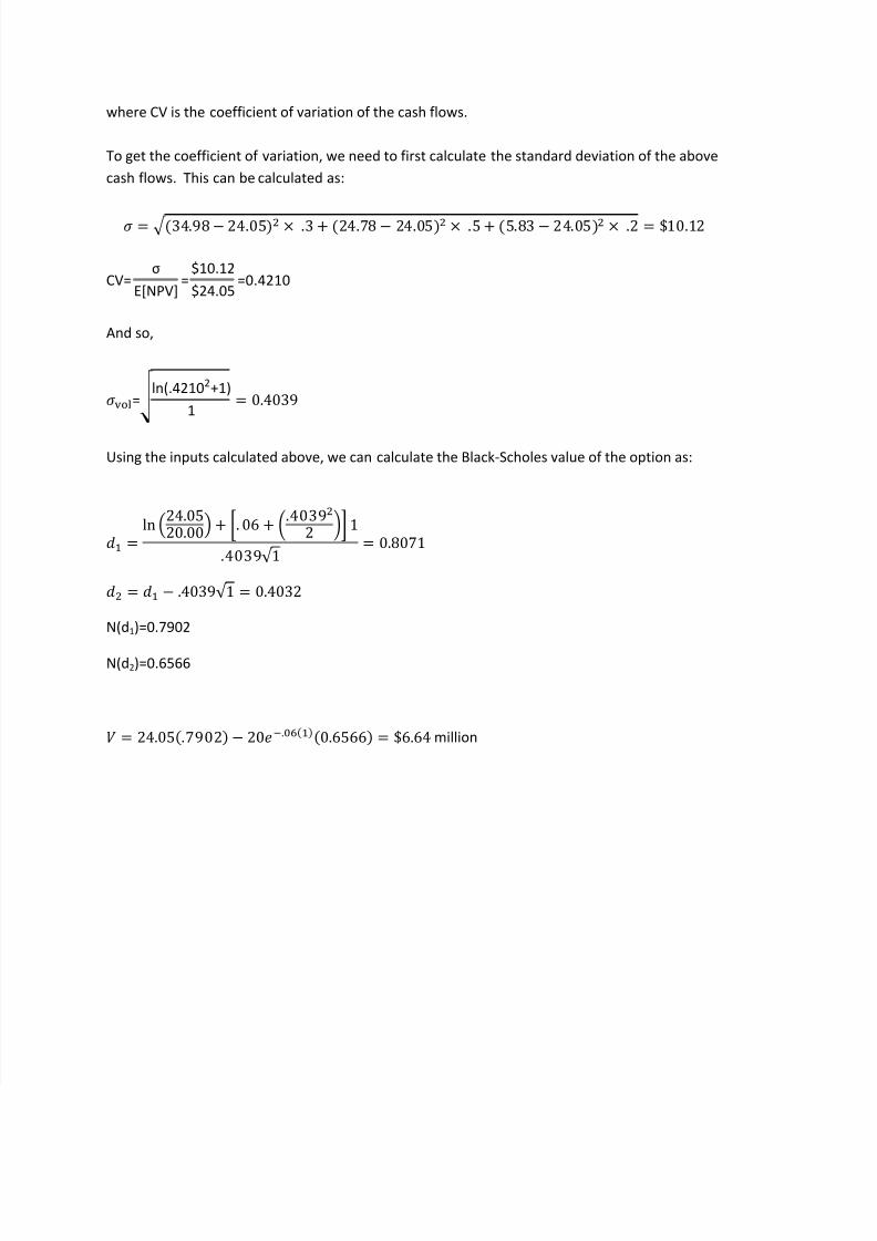
where CV is the coefficient of variation of the cash flows.

To get the coefficient of variation, we need to first calculate the standard deviation of the above

cash flows. This can be calculated as:

= (34.98− 24.05) × .3 + (24.78 − 24.05) × .5+ (5.83 − 24.05) × .2 = $10.12

CV=σ

E[NPV]=

$10.12

$24.05=0.4210

And so,

= ln(.42102+1)

1= 0.4039

Using the inputs calculated above, we can calculate the Black-Scholes value of the option as:

= ln !24.0520.00" + #. 06 + %.40392 &' 1.4039√ 1 = 0.8071

= − .4039√ 1 = 0.4032

N(d1)=0.7902

N(d2)=0.6566

= 24.05(.7902) − 20*.,-()(0.6566) = $6.64million

Documents

Deconstructing a Real Option Problem