Decomposing the stock market intraday dynamics

Physica A 309 (2002) 171–182www.elsevier.com/locate/physa

Decomposing the stock market intraday dynamicsJ. Kwapie%na, S. Drozdza;b;∗, F. Gr-ummerc, F. Rufd, J. Spethc

aInstitute of Nuclear Physics, PL-31-342 Krak�ow, PolandbInstitute of Physics, University of Rzesz�ow, PL-35-310, Poland

cInstitut f$ur Kernphysik, Forschungszentrum J$ulich, D-52425 J$ulich, GermanydWest LB International S.A., 32-34 bd Grande-Duchesse Charlotte, L-2014 Luxembourg

Received 25 September 2001

Abstract

The correlation matrix formalism is used to study temporal aspects of the stock marketevolution. This formalism allows to decompose the 4nancial dynamics into noise as well as intosome coherent repeatable intraday structures. The present study is based on the high-frequencyDeutsche Aktienindex (DAX) data over the time period between November 1997 and Septem-ber 1999, and makes use of both the corresponding returns as well as volatility variations. Oneprincipal conclusion is that a bulk of the stock market dynamics is governed by the uncorre-lated noise-like processes. There exists, however, a small number of components of coherentshort-term repeatable structures in :uctuations that may generate some memory e;ects seen inthe standard autocorrelation function analysis. Laws that govern :uctuations associated with thosevarious components are di;erent, which indicates an extremely complex character of the 4nancial:uctuations. c© 2002 Elsevier Science B.V. All rights reserved.

1. Introduction

One of the great challenges of econophysics is to properly quantify and, followingthis, to explain the nature of 4nancial correlations and :uctuations. The e@cient markethypothesis [1] implies that they are dominated by noise. Indeed, the spectrum of thecorrelation matrix accounting for correlations among the stock market companies agreesvery well [2–4] with the universal predictions of random matrix theory [5,6]. Locationsof extreme eigenvalues di;er, however, from these predictions and thus identify certainsystem-speci4c, non-random properties such as collectivity. In addition, these former

∗ Corresponding author.E-mail address: [email protected] (S. Drozdz).

0378-4371/02/$ - see front matter c© 2002 Elsevier Science B.V. All rights reserved.PII: S 0378 -4371(02)00613 -1

172 J. Kwapie�n et al. / Physica A 309 (2002) 171–182

1998.0 1998.5 1999.0 1999.5

time [y]

4000

5000

6000

7000

DA

X

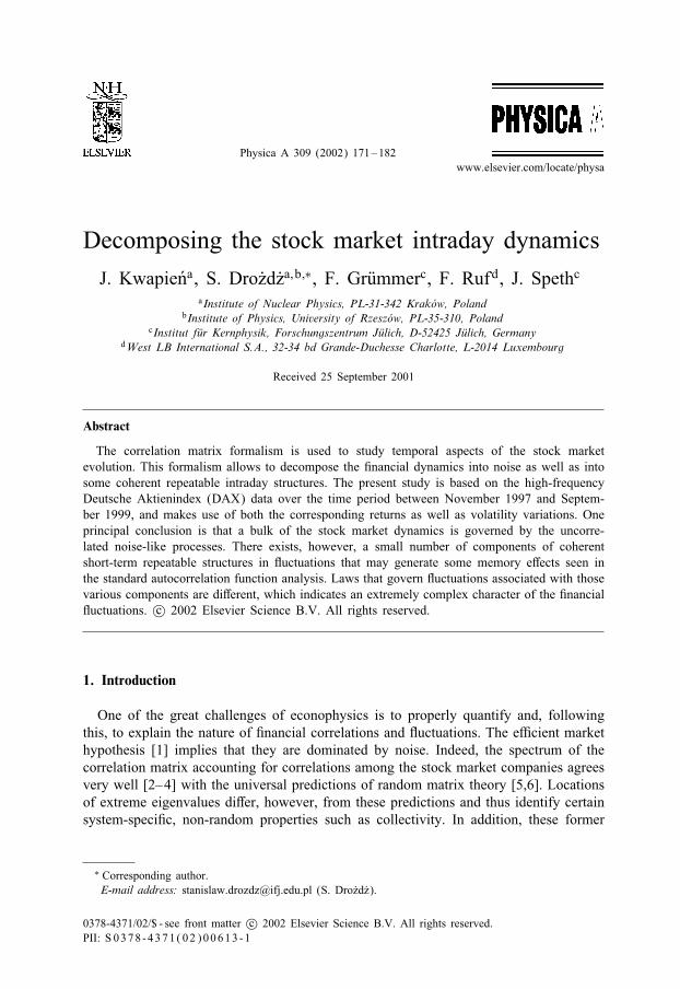
Fig. 1. The DAX in the calendar period November 28, 1997–September 17, 1999.

properties turn out [4,7] to depend on time re:ecting a competitive character of the4nancial dynamics.The character of the 4nancial time correlations is, however, very complex, still poorly

understood and many related issues remain puzzling. The autocorrelation function ofthe 4nancial time series, for instance, drops down to zero within few minutes whichis interpreted as a time horizon of the market ine@ciency [8]. At the same time,however, the correlations in volatility are signi4cantly positive over the time intervalslonger by many orders of magnitude. The fat-tailed return distributions seem to be notL%evy stable [9] on short time scales, but on longer time scales it appears di@cult toidentify their convergence to a Gaussian as expected from the central limit theorem.In addressing this sort of issues below we use the concept of the correlation matrixwhose entries are constructed from the time series of price changes representing theconsecutive trading days. The method focuses then entirely on the time correlations andtheir potential existence can parallelly be detected on various time scales. Analogousmethodology has already been successfully applied [10] to extract from noise somerepeatable structures in the brain sensory response, and its somewhat similar variant,the correlation matrix of the delay matrix, to study the business cycles of economics[11]. The present study is an extension of our recent work [12] and is based on anexample of high-frequency (15 s) recordings [13]. As it can be seen from Fig. 1,this is an interesting period which comprises the whole richness of the stock marketdynamics like strong increases and decreases, and even a clearly identi4able hierarchyof the log-periodic structures [14].

J. Kwapie�n et al. / Physica A 309 (2002) 171–182 173

2. De�niton of correlations

In the present application the entries of the correlation matrix are constructed fromthe time-series g�(ti) of normalized price returns representing the consecutive tradingdays labelled by �. Starting from the original price time-series x�(t) these are de4nedas

g�(ti) =G�(ti)− 〈G�(ti)〉t

�(G�); �(G�) =

√〈G2

�(t)〉t − 〈G�(t)〉2t (1)

with

G�(ti) = ln x�(ti + )− ln x�(ti) � x�(ti + )− x�(ti)x�(ti)

; (2)

where is the time-lag and 〈: : :〉t denotes averaging over time.The result is N time series g�(ti) of length T (the number of records during the

day), i.e. an N × T matrix M. The correlation matrix can then be de4ned as

C = (1=T )MMT : (3)

Its entries C�;�′ are thus labelled by the pairs of di;erent days. By diagonalizing C,

Cvk = �kvk ; (4)

one obtains the eigenvalues �k (k = 1; : : : ; N ) and the corresponding eigenvectorsvk = {vk�}.A useful null hypothesis is provided by the limiting case of entirely random

correlations. In this case the density of eigenvalues �C(�) de4ned as

�C(�) =1N

dn(�)d�

; (5)

where n(�) is the number of eigenvalues of C less than �, is known analytically [15],and reads

�C(�) =Q

2��2

√(�max − �)(�− �min)

�;

�maxmin = �2(1 + 1=Q ± 2

√1=Q) (6)

with �min6 �6 �max, Q=T=N¿ 1, and where �2 is equal to the variance of the timeseries which in our case equals unity.

3. Deutsche Aktienindex (DAX) time correlations

As mentioned above our related study is based on the DAX recordings with thefrequency of 15 s during the period between November 28, 1997 and September 17,1999. After this last date the DAX was traded signi4cantly longer during the tradingday. By taking the DAX intraday 15 s variation between the trading time 9:03 and 17:10which corresponds to T =1948, and rejecting several days with incomplete recordings,one then obtains N = 451 complete and equivalent time series representing di;erent


0 5 10 150

0.3

0.6

0.9

λ

ρ C (λ

)

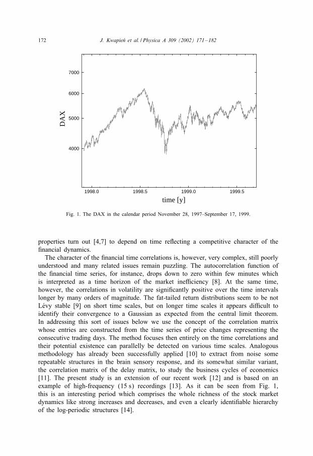
Fig. 2. The probability density (histogram) of the eigenvalues of the correlation matrix C calculated fromthe DAX time series of 15 s returns during the calendar period November 28, 1997–September 17, 1999.The null hypothesis of purely random correlations formulated in terms of Eq. (6) is indicated by the dashedline.

trading days during this calendar period. Using this set of data we then construct the451× 451 matrix C.One characteristic which is of interest is the structure of the eigenspectrum. The

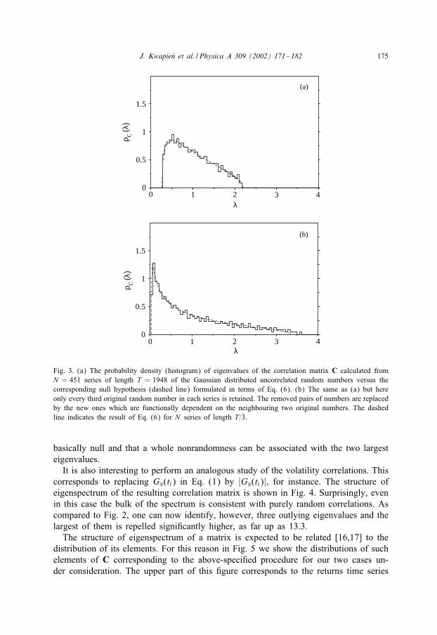
resulting probability density of eigenvalues, shown in Fig. 2, displays a very interest-ing structure. There exist two almost degenerate eigenvalues visibly repelled from thebulk of the spectrum, i.e., well above �max (for Q = 1948=451; �max ≈ 2:19) whichindicates that the dynamics develops certain time-speci4c repeatable structures in theintraday trading. The bulk of the spectrum, however, agrees remarkably well withthe bounds prescribed by purely random correlations. This indicates that the statisticalneighbouring recordings in our time series of 15 s DAX returns share essentially nocommon information.A signi4cance of this result can be evaluated by the following numerical experi-

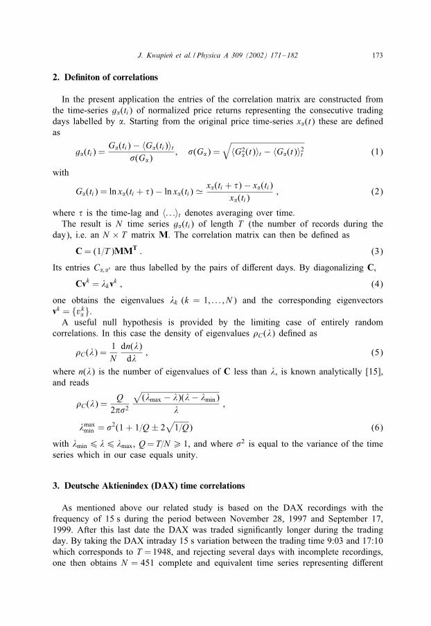
ment. From a Gaussian distribution we draw N = 451 series xn(i) (n = 1; : : : ; N ) ofrandom numbers of length T = 1948 (i = 1; : : : ; T ) and determine the spectrum of theresulting correlation matrix. The result (histogram) versus the corresponding theoret-ical result expressed by Eq. (6) is shown in the upper part of Fig. 3. As expected,the agreement is unqestionable. In the second step, in each previous series we retainonly every third number, e.g., xn(1); xn(4); : : : . This omission is compensated by in-sertion between every two remaining original numbers, say xn(i) and xn(i + 3), thetwo new xn(i + 1); xn(i + 2) numbers such that they are functionally (here linearly)dependent on xn(i) and xn(i + 3). The net result is the same number of N series ofthe same length T as before, thus Q = T=N formally remains unchanged. The struc-ture of eigenspectrum of the corresponding correlation matrix, which is shown in thelower part of Fig. 3, changes, however, completely. In fact, it now perfectly agreeswith the theoretical formula of Eq. (6) but for the three times shorter (T=3) series,i.e., it nicely re:ects a real information content. From this we can conclude thata common information shared by neighbouring events in our DAX time series is


λ

ρ C (λ

)

00

0.5

1

1.5

(a)

1 2 3 4

0

0.5

1

1.5

(b)

0 1 2 3 4λ

ρ C (λ

)

Fig. 3. (a) The probability density (histogram) of eigenvalues of the correlation matrix C calculated fromN = 451 series of length T = 1948 of the Gaussian distributed uncorrelated random numbers versus thecorresponding null hypothesis (dashed line) formulated in terms of Eq. (6). (b) The same as (a) but hereonly every third original random number in each series is retained. The removed pairs of numbers are replacedby the new ones which are functionally dependent on the neighbouring two original numbers. The dashedline indicates the result of Eq. (6) for N series of length T=3.

basically null and that a whole nonrandomness can be associated with the two largesteigenvalues.It is also interesting to perform an analogous study of the volatility correlations. This

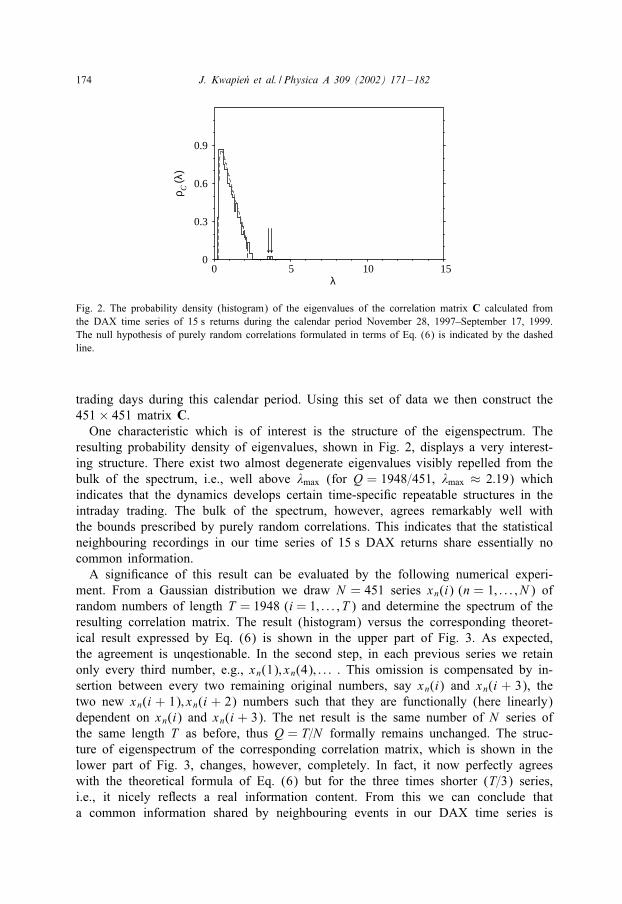
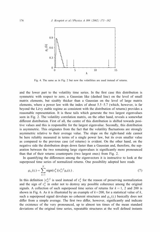
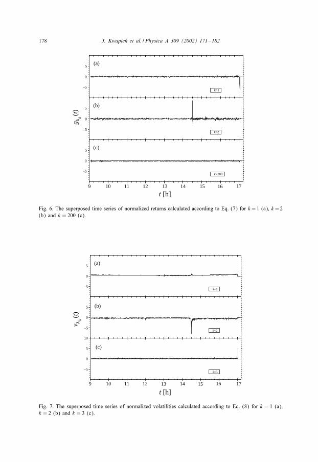
corresponds to replacing G�(ti) in Eq. (1) by |G�(ti)|, for instance. The structure ofeigenspectrum of the resulting correlation matrix is shown in Fig. 4. Surprisingly, evenin this case the bulk of the spectrum is consistent with purely random correlations. Ascompared to Fig. 2, one can now identify, however, three outlying eigenvalues and thelargest of them is repelled signi4cantly higher, as far up as 13.3.The structure of eigenspectrum of a matrix is expected to be related [16,17] to the

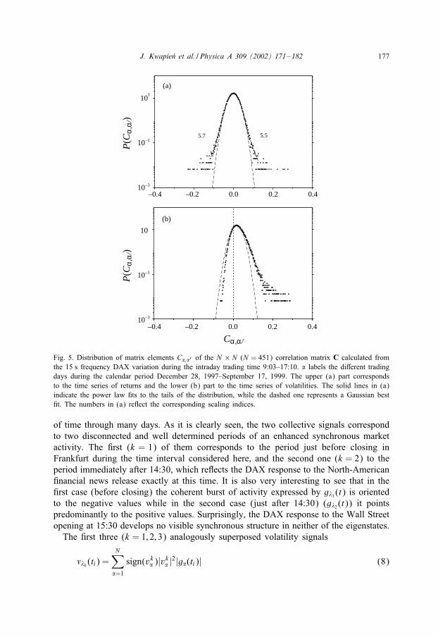
distribution of its elements. For this reason in Fig. 5 we show the distributions of suchelements of C corresponding to the above-speci4ed procedure for our two cases un-der consideration. The upper part of this 4gure corresponds to the returns time series


0 5 10 150

0.3

0.6

0.9

λ

ρ C (λ

)

Fig. 4. The same as in Fig. 2 but now the volatilities are used instead of returns.

and the lower part to the volatility time series. In the 4rst case this distribution issymmetric with respect to zero, a Gaussian like (dashed line) on the level of smallmatrix elements, but sizably thicker than a Gaussian on the level of large matrixelements, where a power law with the index of about 5.5–5.7 (which, however, is farbeyond the L%evy stable regime as consistent with the distribution of returns) provides areasonable representation. It is these tails which generate the two largest eigenvaluesseen in Fig. 2. The volatility correlation matrix, on the other hand, reveals a somewhatdi;erent distribution. First of all, the centre of this distribution is shifted towards posi-tive values and this is responsible for the largest eigenvalue. Secondly, this distributionis asymmetric. This originates from the fact that the volatility :uctuations are stronglyasymmetric relative to their average value. The slope on the right-hand side cannotbe here reliably measured in terms of a single power law, but its even smaller valueas compared to the previous case (of returns) is evident. On the other hand, on thenegative side the distribution drops down faster than a Gaussian and, therefore, the sep-aration between the two remaining large eigenvalues is signi4cantly more pronouncedthan that of their returns counterparts (two largest ones) from Fig. 2.In quantifying the di;erences among the eigenvectors it is instructive to look at the

superposed time series of normalized returns. One possibility adopted here reads

g�k (ti) =N∑�=1

sign(vk� )|vk� |2g�(ti) : (7)

In this de4nition |vk� |2 is used instead of vk� for the reason of preserving normalizationand the sign of vk� in order not to destroy any possible coherence among the originalsignals. A collection of such superposed time series of returns for k = 1, 2 and 200 isshown in Fig. 6. As it is illustrated by an example of k=200, for a statistical value of k,such a superposed signal develops no coherent structures and g�k (ti) basically does notdi;er from a simple average. The 4rst two di;er, however, signi4cantly and indicatethe existence of the very pronounced, up to almost ten times of the mean standarddeviations of the original time series, repeatable structures at the well de4ned instants


–0.4 –0.2 0.0 0.2 0.410 –3

–1

101

5.7 5.5

(a)

10P(C

α,α

/)

(b)

10 –3

–1

10

10P(C

α,α

/)

–0.4 –0.2 0.0 0.2 0.4

Cα,α/

Fig. 5. Distribution of matrix elements C�;�′ of the N × N (N = 451) correlation matrix C calculated fromthe 15 s frequency DAX variation during the intraday trading time 9:03–17:10. � labels the di;erent tradingdays during the calendar period December 28, 1997–September 17, 1999. The upper (a) part correspondsto the time series of returns and the lower (b) part to the time series of volatilities. The solid lines in (a)indicate the power law 4ts to the tails of the distribution, while the dashed one represents a Gaussian best4t. The numbers in (a) re:ect the corresponding scaling indices.

of time through many days. As it is clearly seen, the two collective signals correspondto two disconnected and well determined periods of an enhanced synchronous marketactivity. The 4rst (k = 1) of them corresponds to the period just before closing inFrankfurt during the time interval considered here, and the second one (k = 2) to theperiod immediately after 14:30, which re:ects the DAX response to the North-American4nancial news release exactly at this time. It is also very interesting to see that in the4rst case (before closing) the coherent burst of activity expressed by g�1 (t) is orientedto the negative values while in the second case (just after 14:30) (g�2 (t)) it pointspredominantly to the positive values. Surprisingly, the DAX response to the Wall Streetopening at 15:30 develops no visible synchronous structure in neither of the eigenstates.The 4rst three (k = 1; 2; 3) analogously superposed volatility signals

��k (ti) =N∑�=1

sign(vk� )|vk� |2|g�(ti)| (8)


9 10 11 12 13 14 15

–5

0

5

k=200

–5

0

5

k=2

–5

0

5

k=1

t [h]

(a)

(b)

(c)

g λ k(t

)

16 17

Fig. 6. The superposed time series of normalized returns calculated according to Eq. (7) for k=1 (a), k=2(b) and k = 200 (c).

9 10 11 12 13 14 15 16 17

–5

0

5

10

k=3

–5

0

5

k=2

–5

0

5

k=1

t [h]

(a)

(b)

(c)

v λ k(t

)

Fig. 7. The superposed time series of normalized volatilities calculated according to Eq. (8) for k = 1 (a),k = 2 (b) and k = 3 (c).


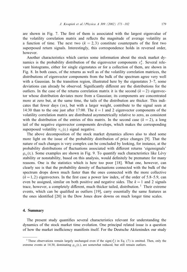
are shown in Fig. 7. The 4rst of them is associated with the largest eigenvalue ofthe volatility correlation matrix and re:ects the magnitude of average volatility asa function of time. The next two (k = 2; 3) constitute counterparts of the 4rst twosuperposed return signals. Interestingly, this correspondence holds in reversed order,however.Another characteristics which carries some information about the stock market dy-

namics is the probability distribution of the eigenvector components vk� . Several rele-vant histograms, either for single eigenstates or for a collection of them, are shown inFig. 8. In both cases, of the returns as well as of the volatility correlation matrices, thedistributions of eigenvector components from the bulk of the spectrum agree very wellwith a Gaussian. In the transition region, illustrated here by the eigenstates 3–7, somedeviations can already be observed. Signi4cantly di;erent are the distributions for theoutliers. In the case of the returns correlation matrix it is the second (k =2) eigenvec-tor whose distribution deviates more from a Gaussian; its components are concentratedmore at zero but, at the same time, the tails of the distribution are thicker. This indi-cates that fewer days (�s), but with a larger weight, contribute to the signal seen at14:30 than to the one just after 17:00. The k =1 and 2 eigenvector components of thevolatility correlation matrix are distributed asymmetrically relative to zero, as consistentwith the distribution of the entries of this matrix. In the second case (k = 2), a longtail of the negative eigenvector components develops, which makes the correspondingsuperposed volatility ��2 (ti) signal negative.The above decomposition of the stock market dynamics allows also to shed some

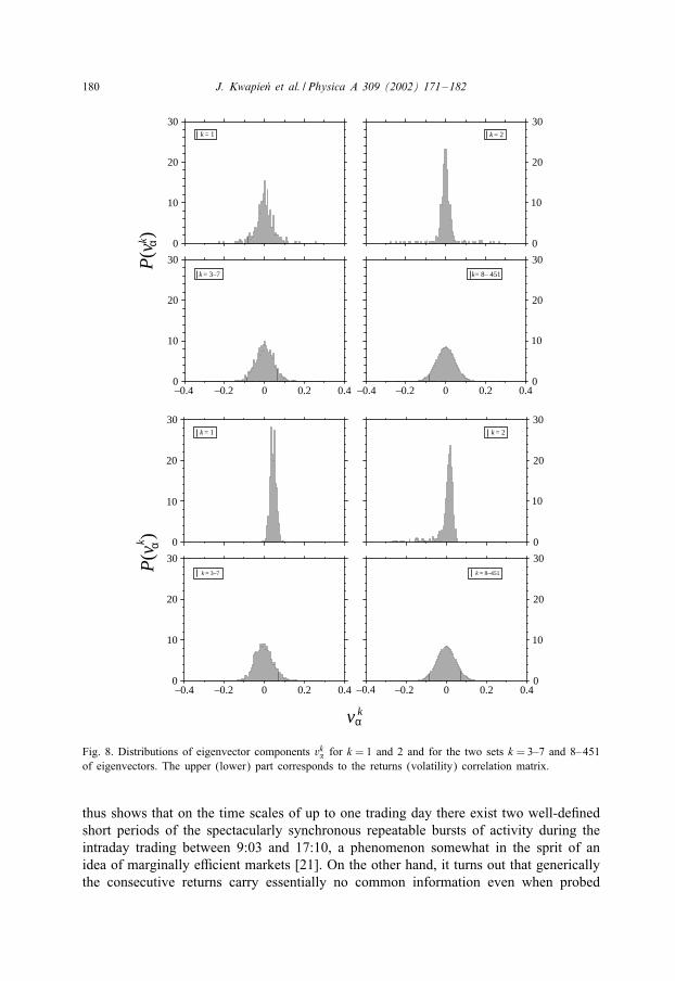
more light on the issue of the probability distribution of price changes [9]. That thenature of such changes is very complex can be concluded by looking, for instance, at theprobability distributions of :uctuations associated with di;erent returns ‘eigensignals’g�k (ti). Some examples are shown in Fig. 9. To quantify such characteristics like L%evystability or nonstability, based on this analysis, would de4nitely be premature for manyreasons. One is the statistics which is here too poor [18]. What one, however, canclearly see is that the probability density of :uctuations connected with the bulk of thespectrum drops down much faster than the ones connected with the more collective(k=1; 2) eigenvectors. In the 4rst case a power law index, of the order of 5.8–5.9, caneven be assigned, similar on both positive and negative sides. The k =1 and 2 signalstrace, however, a completely di;erent, much thicker tailed, distribution. 1 Their extremeevents, which can be quali4ed as outliers [19], carry essentially the same features asthe ones identi4ed [20] in the Dow Jones draw downs on much longer time scales.

4. Summary

The present study quanti4es several characteristics relevant for understanding thedynamics of the stock market time evolution. One principal related issue is a questionof how the market ine@ciency manifests itself. For the Deutsche Aktienindex our study

1 These observations remain largely unchanged even if the sign(vk�) in Eq. (7) is omitted. Then, only theextreme events at 14:30, dominating g�2 (ti), are somewhat reduced, but still remain outliers.


–0.4 –0.2 0 0.2 0.40

10

20

30k = 3–7

0

10

20

30k = 1

–0.4 –0.2 0 0.2 0.40

10

20

30k = 8– 451

0

10

20

30k = 2

P(v

k α )

–0.4 –0.2 0 0.2 0.40

10

20

30k = 3–7

0

10

20

30k = 1

–0.4 –0.2 0 0.2 0.40

10

20

30k = 8–451

0

10

20

30k = 2

vα

P(v

k α)

k

Fig. 8. Distributions of eigenvector components vk� for k = 1 and 2 and for the two sets k = 3–7 and 8–451of eigenvectors. The upper (lower) part corresponds to the returns (volatility) correlation matrix.

thus shows that on the time scales of up to one trading day there exist two well-de4nedshort periods of the spectacularly synchronous repeatable bursts of activity during theintraday trading between 9:03 and 17:10, a phenomenon somewhat in the sprit of anidea of marginally e@cient markets [21]. On the other hand, it turns out that genericallythe consecutive returns carry essentially no common information even when probed


10 –2 10 –1 10 0 10 110

–5

10 –3

10 –1

101

k = 11– 451k = 2k = 1

5.8

(+)

gλ k

P(g

λ k)

10 –2 10 –1 100

10110

–5

10 –3

10 –1

10 1

k = 11– 451k = 2k = 1

5.9

(–)

P(g

λ k)

gλ k

Fig. 9. Probability density functions of :uctuations of the superposed returns as expressed by Eq. (7). Squarescorrespond to k = 1, triangles to k = 2 and the circles to the average of k = 11–451. Both positive (upperpart) and negative (lower part) sides of those distributions are shown.

with the frequency of 15 s. The :uctuations associated with the so identi4ed distinctcomponents are governed by the di;erent laws which re:ects an extreme complexityof the stock market dynamics.

References

[1] P.A. Samuelson, Ind. Manage. Rev. 6 (1965) 41.[2] L. Laloux, P. Cizeau, J.-.P. Bouchaud, M. Potters, Phys. Rev. Lett. 83 (1999) 1467.


[3] V. Plerou, P. Gopikrishnan, B. Rosenow, L.A.N. Amaral, H.E. Stanley, Phys. Rev. Lett. 83 (1999)1471.

[4] S. Drozdz, F. Gr-ummer, A.Z. G%orski, F. Ruf, J. Speth, Physica A 287 (2000) 440.[5] E.P. Wigner, Ann. Math. 53 (1951) 36.[6] M.L. Mehta, Random Matrices, Academic Press, Boston, 1999.[7] S. Drozdz, F. Gr-ummer, F. Ruf, J. Speth, Physica A 294 (2001) 226.[8] J.Y. Campbell, A.W. Lo, A. Craig MacKinley, The Econometrics of Financial Markets, Princeton

University Press, Princeton, NJ, 1997.[9] R.N. Mantegna, H. Eugene Stanley, An Introduction to Econophysics: Correlations and Complexity in

Finance, University Press, Cambridge, 2000.[10] J. Kwapie%n, S. Drozdz, A.A. Ioannides, Phys. Rev. E 62 (2000) 5557.[11] P. Ormerod, C. Moun4eld, Physica A 280 (2000) 497.[12] S. Drozdz, J. Kwapie%n, F. Gr-ummer, F. Ruf, J. Speth, Quantifying the dynamics of 4nancial correlations,

cond-mat=0102402, Physica A 299 (2001) 144.[13] H. Goeppl, Data from Karlsruher Kapitalmarktdatenbank (KKMDB), Institut f-ur Entscheidungstheorie

u. Unternehmensforschung, Universit-at Karlsruhe (TH).[14] S. Drozdz, F. Ruf, J. Speth, M. W%ojcik, Eur. Phys. J. B 10 (1999) 589.[15] A. Edelman, SIAM J. Matrix Anal. Appl. 9 (1988) 543;

A.M. Sengupta, P.P. Mitra, Phys. Rev. E 60 (1999) 3389.[16] S. Drozdz, S. Nishizaki, J. Speth, M. W%ojcik, Phys. Rev. E 57 (1998) 4016.[17] S. Drozdz, F. Gr-ummer, F. Ruf, J. Speth, Dynamics of correlations in the stock market, in: H. Takayasu

(Ed.), Empirical Science of Financial Fluctuations, Springer, Tokyo, 2002, pp. 41–50;S. Drozdz, F. Gr-ummer, F. Ruf, J. Speth, in: H. Takayasu (Ed.), Empirical Science of FinancialFluctuations, Springer, Tokyo, 2001, in press.

[18] R. Weron, Int. J. Modern Phys. C 12 (2001) 206.[19] V.S. Lvov, A. Pomyalov, I. Procaccia, Phys. Rev. E 63 (2001) 056118.[20] A. Johansen, D. Sornette, Eur. Phys. J. B 9 (1999) 167.[21] Y.-C. Zhang, Physica A 269 (1999) 30.

Documents

Decomposing the stock market intraday dynamics