Decision and Regression Tree Learning

CS 586Prepared by Jugal Kalita

With help from Tom Mitchell’s Machine Learning, Chapter 3Alpaydin’s Ethem Introduction to Machine Learning, Chapter 9Jang, Sun and Mizutani’s Neuro-Fuzzy and Soft Computing,

Chapter 14Dan Steinberg, CART: Classification and Regression Trees,

2009

Training Examples

Suppose we are given a table of training examples. HerePlayTennis is the concept to be learned.

Day Outlook Temperature Humidity Wind PlayTennisD1 Sunny Hot High Weak NoD2 Sunny Hot High Strong NoD3 Overcast Hot High Weak YesD4 Rain Mild High Weak YesD5 Rain Cool Normal Weak YesD6 Rain Cool Normal Strong NoD7 Overcast Cool Normal Strong YesD8 Sunny Mild High Weak NoD9 Sunny Cool Normal Weak Yes

D10 Rain Mild Normal Weak YesD11 Sunny Mild Normal Strong YesD12 Overcast Mild High Strong YesD13 Overcast Hot Normal Weak YesD14 Rain Mild High Strong No

1

A Possible Decision Tree for P layTennis

Outlook

Overcast

Humidity

NormalHigh

No Yes

Wind

Strong Weak

No Yes

Yes

RainSunny

From Page 53 of Mitchell

2

Decision or Regression Trees

• A decision tree solves a classification problem based onlabeled examples. It is a supervised learning technique.

• Each internal node tests an attribute.• Each branch corresponds to attribute value.• Each leaf node assigns a classification.• Although in this example, all attribute values are discrete,

the values can be continuous as well.• If the target attribute (i.e., the attribute to be learned, here

P layTennis) is continuous, the tree that results is called aregression tree. Otherwise, it is a decision tree.

• In a regression tree, the leaf nodes may have specific val-ues for the concept or a function to compute the value ofthe target attribute.

3

What does a Decision or Regression Tree Represent?

• We can traverse the decision or regression tree from rootdown to classify an unseen example.

• A decision or regression tree represents a disjunct of con-juncts. The decision tree given earlier corresponds to theexpression(Outlook = Sunny ^Humidity = Normal)

_ (Outlook = Overcast)

_ (Outlook = Rain ^Wind = Weak)

• A decision or regression tree can be expressed in terms ofsimple rules as well.

4

Representing a Decision or RegressionTree in Rules

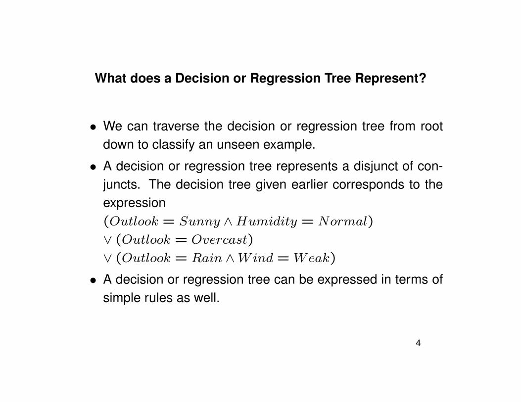
• We can express the example decision tree in terms of rules.• The last or default rule may or may not be necessary, de-

pending on how rules are processed.• Representing knowledge in readable rules is convenient.

If (Outlook = Sunny ^ Humidity = Normal), thenP layTennisIf (Outlook = Overcast), then P layTennisIf (Outlook = Rain^Wind = Weak), then P layTennisOtherwise, ¬P layTennis

• The conclusion of each rule obtained from a decision treeis a value of the target attribute from a small set of pos-sible values. The conclusion of each rule obtained from aregression tree is a value of the target attribute or a functionto compute the value of the target attribute.

5

Basic Issues in Decision or Regression Tree Learning

• Under what situations can we use a decision tree for classi-fication? Or a regression tree for regression?

• How do we build a decision or regression tree from thedata?

• Which one of the many possible decision (or, regression)trees do we build and why?

6

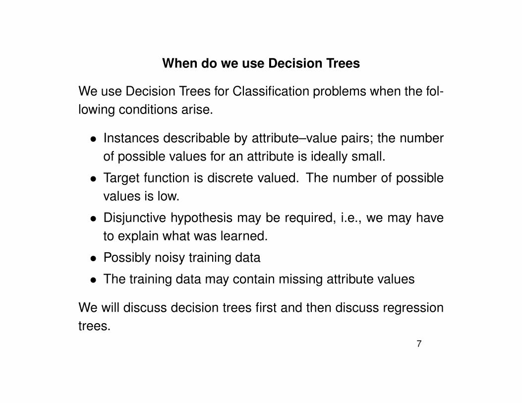
When do we use Decision Trees

We use Decision Trees for Classification problems when the fol-lowing conditions arise.

• Instances describable by attribute–value pairs; the numberof possible values for an attribute is ideally small.

• Target function is discrete valued. The number of possiblevalues is low.

• Disjunctive hypothesis may be required, i.e., we may haveto explain what was learned.

• Possibly noisy training data

• The training data may contain missing attribute values

We will discuss decision trees first and then discuss regressiontrees.

7

Examples of usage of Decision Trees

• Equipment or medical diagnosis

• Credit risk analysis

• Classifying living species based on characterisitics

• Stock trading

• Intrusion Detection

• Speech Processing

• Classifying Mammography data, etc.

8

Entropy in Data: A Measure of Impurity of a Set of Data

• Entropy in a collection of data samples represents the amountof impurity or chaos in the data.

• We will measure entropy by considering the classes datasamples in a set belong to.

• Entropy in a set of data items should be 0 if there is nochaos or impurity in the data. In other words, if all items inthe set belong to the same class, entropy should be 0.

• Entropy in a set of data belonging to several classes shouldbe 1 if the data is equally divided into several classes. Forexamples, if we have two classes and our samples in a setare equally distributed in the two classes, entropy is 1.

9

Computing Entropy in Data

Entropy(S)

1.0

0.5

0.0 0.5 1.0

p+

• Let T be a set of training examples belonging to two classes,+ and �.

• p� is the proportion of positive examples in T

• p is the proportion of negative examples in T

• Entropy measures the impurity of T

Entropy(T ) = �p� log

2

p� � p log

2

p 10

Entropy in Information Theory

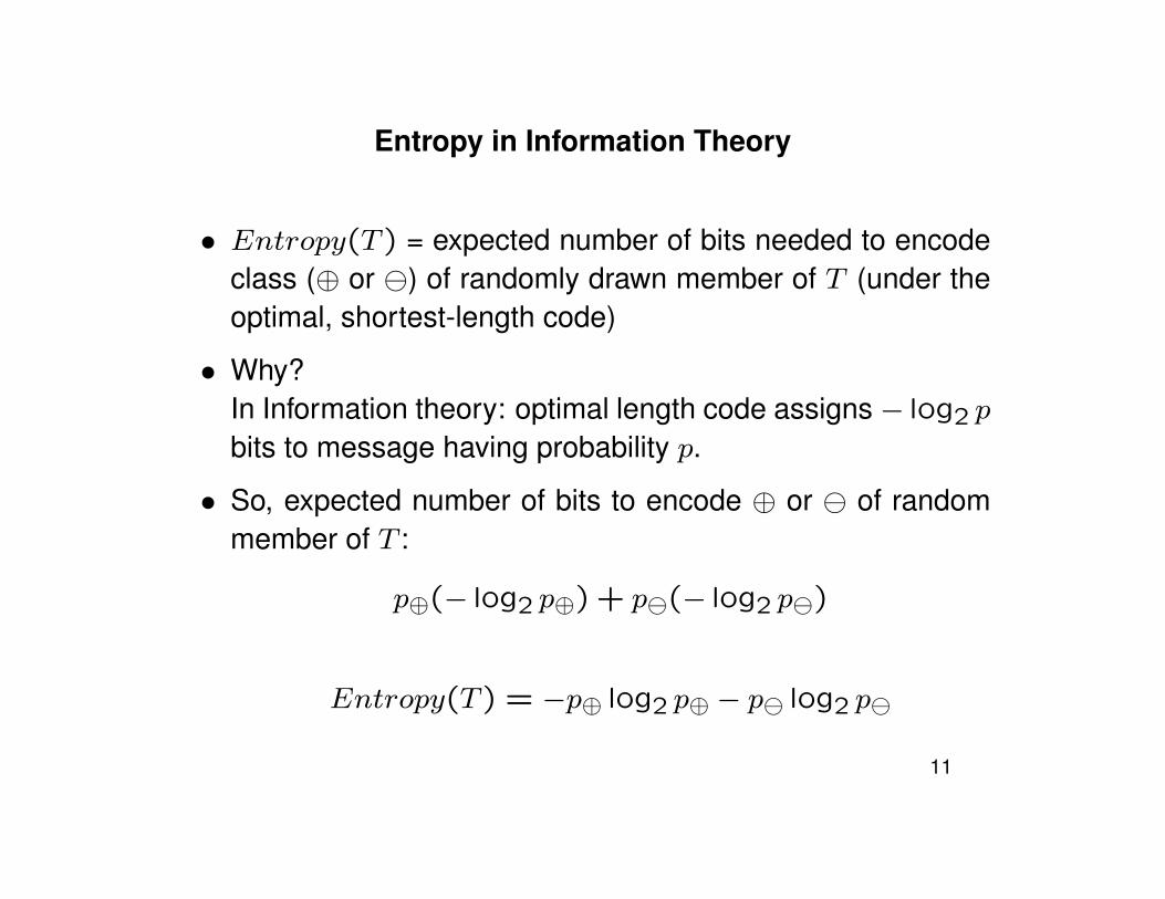
• Entropy(T ) = expected number of bits needed to encodeclass (� or ) of randomly drawn member of T (under theoptimal, shortest-length code)

• Why?In Information theory: optimal length code assigns � log

2

pbits to message having probability p.

• So, expected number of bits to encode � or of randommember of T :

p�(� log

2

p�) + p (� log

2

p )

Entropy(T ) = �p� log

2

p� � p log

2

p

11

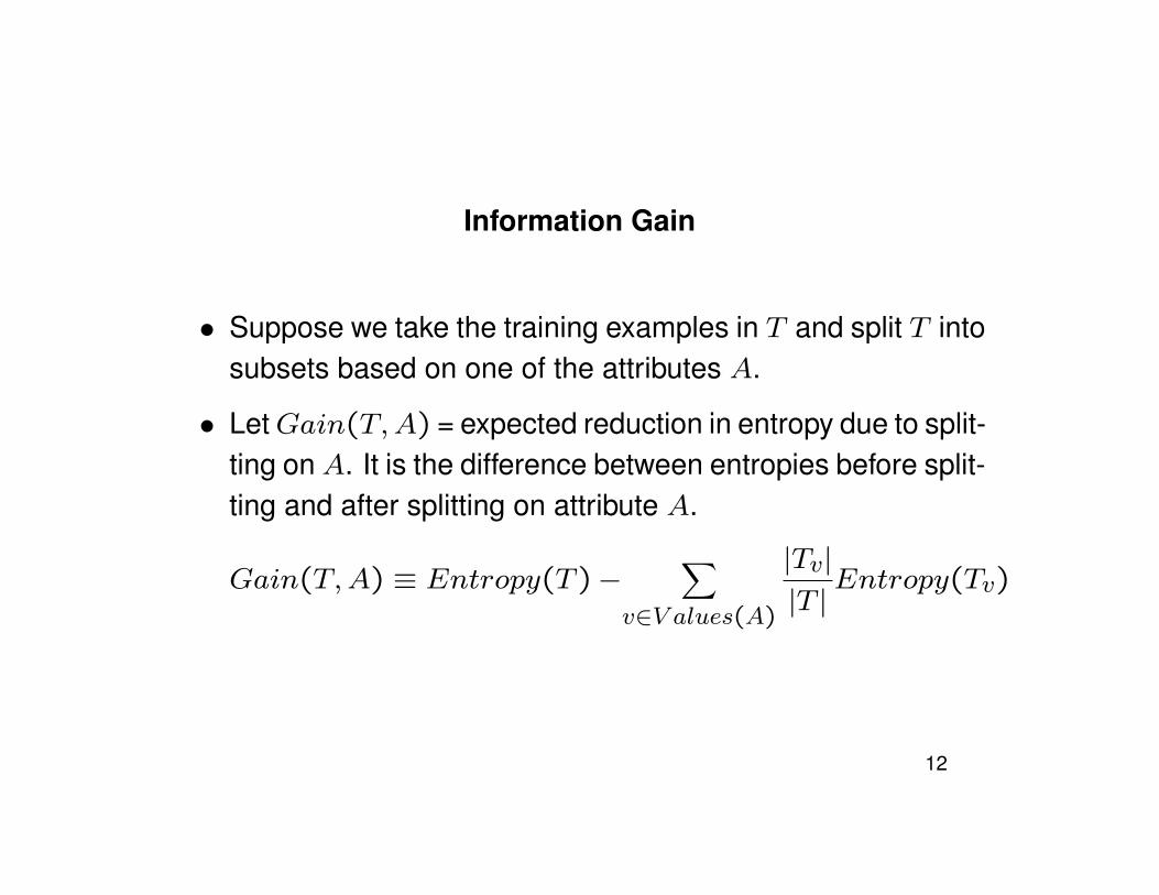
Information Gain

• Suppose we take the training examples in T and split T intosubsets based on one of the attributes A.

• Let Gain(T,A) = expected reduction in entropy due to split-ting on A. It is the difference between entropies before split-ting and after splitting on attribute A.

Gain(T,A) ⌘ Entropy(T )�X

v2V alues(A)

|Tv||T |

Entropy(Tv)

12

Selecting the First Attribute

Which attribute is the best classifier?

High Normal

Humidity

[3+,4-] [6+,1-]

Wind

Weak Strong

[6+,2-] [3+,3-]

= .940 - (7/14).985 - (7/14).592 = .151

= .940 - (8/14).811 - (6/14)1.0 = .048

Gain (S, Humidity ) Gain (S, )Wind

=0.940E =0.940E

=0.811E=0.592E=0.985E =1.00E

[9+,5-]S:[9+,5-]S:

13

Selecting the First Attribute

Gain(T,Outlook) = 0.246

Gain(T,Humidity) = 0.151

Gain(T,Wind) = 0.048

Gain(T, Temperature) = 0.029

Choose Outlook as the root attribute since it gives the mostinformation gain.

14

Selecting the Next Attribute

TSunny = {D1, D2, D8, D9, D11}Gain(Tsunny,Humidity) = .970� (3/5)0.0� (2/5)0.0 = .970

Gain(Tsunny, T emperature) = .970� (2/5)0.0� (1/5)0.0 = .570Gain(Tsunny,Wind) = .970� (2/5)1.0� (3/5)0.918 = .019

Choose Humidity as next attribute under Sunny because it gives most information gain.

From Page 61 of Mitchell.

15

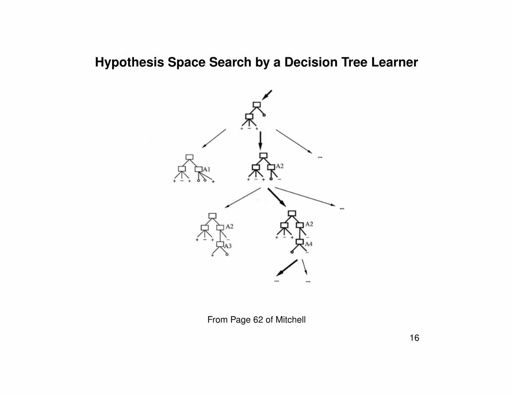
Hypothesis Space Search by a Decision Tree Learner

From Page 62 of Mitchell

16

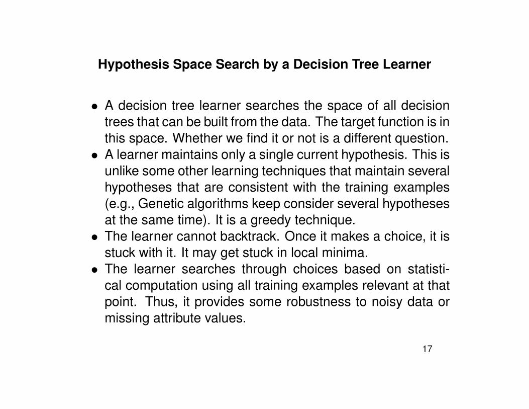
Hypothesis Space Search by a Decision Tree Learner

• A decision tree learner searches the space of all decisiontrees that can be built from the data. The target function is inthis space. Whether we find it or not is a different question.

• A learner maintains only a single current hypothesis. This isunlike some other learning techniques that maintain severalhypotheses that are consistent with the training examples(e.g., Genetic algorithms keep consider several hypothesesat the same time). It is a greedy technique.

• The learner cannot backtrack. Once it makes a choice, it isstuck with it. It may get stuck in local minima.

• The learner searches through choices based on statisti-cal computation using all training examples relevant at thatpoint. Thus, it provides some robustness to noisy data ormissing attribute values.

17

Inductive Bias in Decision Tree Learning

• Inductive Bias: We are searching in the space of trees orequivalently logical formulas that are disjuncts of conjuncts

• Preference for short trees, and for those with high informa-tion gain attributes near the root.

• Occam’s razor: prefer the shortest hypothesis that fits thedata. Why prefer short hypotheses?

– Fewer short hypotheses than long hypotheses.– A short hypothesis that fits data unlikely to be coinci-

dence.– A long hypothesis that fits data might be coincidence.

18

Some Issues in Decision and Regression Tree Learning

• Avoid overfitting the data.• Incorporate continuous-valued attributes.• Other measures for selecting attributes.• Handle training examples with missing attributes.• Handle attributes with different costs.• Univariate, multivariate, or omnivariate trees.• Regression trees. These are like decision trees, but the

target attribute is continuous.• Balancing subtrees.• Testing the hypothesis obtained.

19

Overfitting the training examples

• Consider error of hypothesis h over– training data: errortrain(h)– entire distribution D of data: errorD(h)

• Hypothesis h 2 H overfits training data if there is an alter-native hypothesis h0 2 H such that

errortrain(h) < errortrain(h0)

but

errorD(h) > errorD(h0)

• In other words, h fits the training data better than h0, but hdoes worse on the entire distribution of the data.

20

Overfitting in Decision Tree Learning

0.5

0.55

0.6

0.65

0.7

0.75

0.8

0.85

0.9

0 10 20 30 40 50 60 70 80 90 100

Acc

ura

cy

Size of tree (number of nodes)

On training dataOn test data

As new nodes are added to the decision tree, the accu-racy of the tree over the training examples increased mono-tonically. However, measured over an independent set oftraining examples, the accuracy first increases and then de-creases. From Page 67 of Mitchell.

21

How to Avoid Overfitting

Two possible approaches:

• Stop growing the tree before the tree fits the data perfectly.It is difficult to figure out when to stop.

• Grow full tree, then post-prune. This is the method normallyused.

22

How to select “best” tree

• Use a separate set of examples, distinct from the trainingexamples, to evaluate how post-pruning of nodes from thetree is working. This set is called the validation set.

• Use all the available data for training, but apply a statisti-cal test to estimate whether expanding or pruning a par-ticular node is likely to produce improvement beyond thetraining set. Quinlan (1986) uses a chi-square test to esti-mate whether further expanding a node is likely to improveperformance over the entire distribution, not just the trainingexamples.

• Use an explicit measure of complexity for encoding trainingexamples and the decision tree, halting growth when thisencoding size is minimized. It uses the so-called Minimum

Description Length principle.

23

Reduced-Error Pruning

• It is one of the most common ways to prune a fully growndecision tree.

• Split data into training and validation set

• Do until further pruning is harmful:

– Evaluate impact on validation set of pruning each pos-sible node (plus those below it); i.e., pick a node (insome traversal order, e.g., reverse depth-first order) andremove it with all branches below it, and examine howwell the new tree classifies examples in the validationset.

– Greedily remove the one that most improves validation

set accuracy24

• produces smallest version of most accurate subtree

Note: Some people use three independent sets of data: training set for train-

ing the decision tree, validation set for pruning, and test set for testing on a

pruned tree. Assuming the data elements are randomly distributed, the same

regularities do not occur in the three sets.

Effect of Reduced-Error Pruning

0.5

0.55

0.6

0.65

0.7

0.75

0.8

0.85

0.9

0 10 20 30 40 50 60 70 80 90 100

Acc

ura

cy

Size of tree (number of nodes)

On training dataOn test data

On test data (during pruning)

From Page 70 of Mitchell.

25

Rule Post-Pruning

• Grow the tree till overfitting occurs.

• Convert tree to equivalent set of rules by creating one rulefor each path from root to a leaf.

• Prune i.e., generalize each rule independently of others byremoving any precondition that results in improving esti-mated accuracy over a test/validation set. Accuracy is mea-sured by what proportion of examples in the test/validationset does the rule cover.

• Sort final rules by estimated accuracy; consider the rules inthis sequence.

26

Pruning Rules

Suppose we have the rule:IF (Outlook = Sunny) and (Humidity = High)THEN P layTennis = No.

• We can consider dropping one antecedent, and then thesecond to see if the accuracy doesn’t become worse.

• In this simple case, dropping an antecedent may not behelpful, but if we have many antecedents (say 5-10 or more),dropping one or more may not affect performance.

• When we evaluate the performance of a rule, we can bepessimistic; it will perform worse with real data than withthe training/test/validation data. We can assume that thedata and thus the rule’s accuracy will be distributed accord-ing to a certain distribution and we assume that the rule’saccuracy will be within a certain confidence level (say 95%).

27

Why Convert Decision Tree to Rules before Pruning?

• Converting to rules allows distinguishing among the differ-ent contexts in which a decision node occurs. Pruning deci-sion regarding an attribute can be made differently for eachpath (or equivalently, rule). In contrast, if the tree itself ispruned, the only two choices are to remove the node or notremove it.

• Converting to rules removes the distinction between attributetests that occur near the root of the tree and those that oc-cur near the leaves. In contrast, if we prune nodes in a tree,we have to make a decision regarding reorganizing the treeif a non-leaf node is pruned and nodes below are kept.

• Rules are easy for people to understand. When rule pre-conditions are pruned, people understand what is actuallybeing pruned better.

28

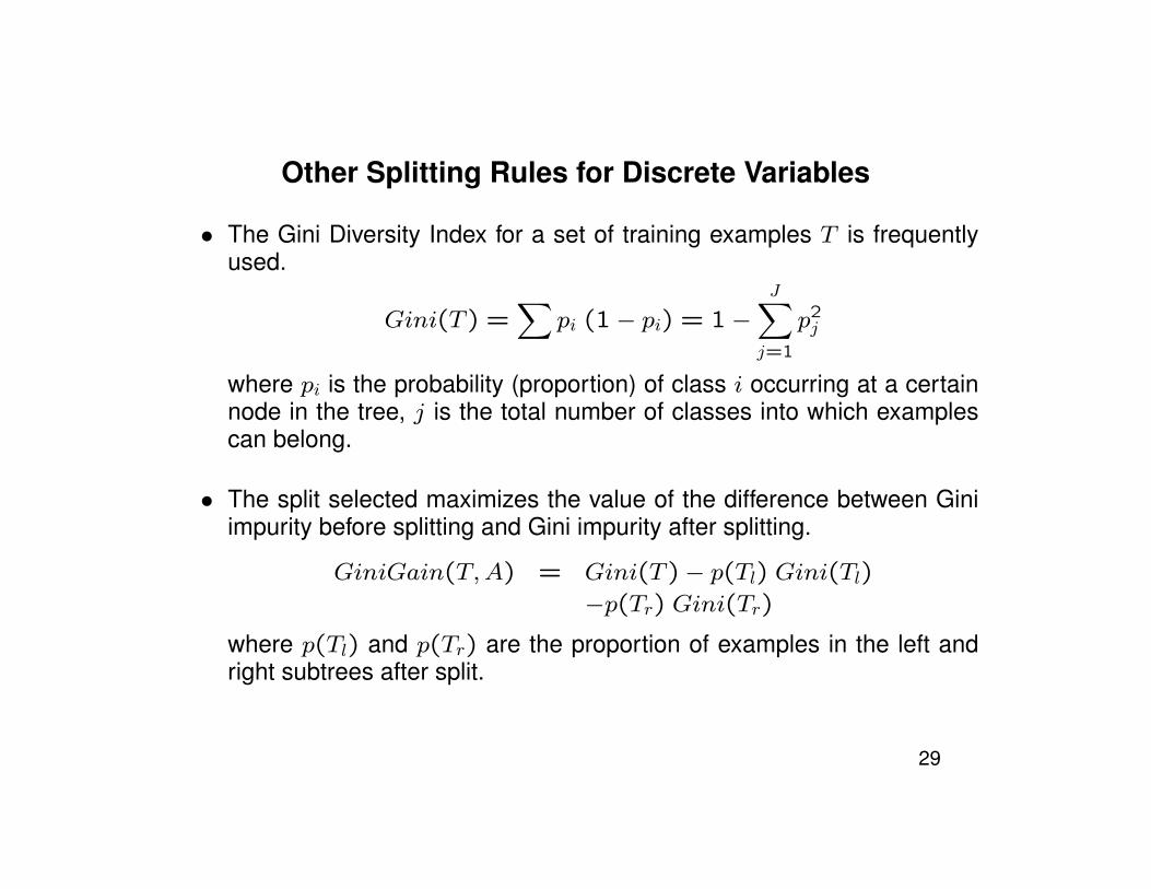
Other Splitting Rules for Discrete Variables

• The Gini Diversity Index for a set of training examples T is frequentlyused.

Gini(T ) =

Xpi (1� pi) = 1�

JX

j=1

p2j

where pi is the probability (proportion) of class i occurring at a certainnode in the tree, j is the total number of classes into which examplescan belong.

• The split selected maximizes the value of the difference between Giniimpurity before splitting and Gini impurity after splitting.

GiniGain(T,A) = Gini(T )� p(Tl) Gini(Tl)

�p(Tr) Gini(Tr)

where p(Tl) and p(Tr) are the proportion of examples in the left andright subtrees after split.

29

Comparing Entropy and Gini Index of Diversity

As we can see, the two functions are not very different. Here J is the total number of

classes. From Page 409 of Jang et al.

30

Other Splitting Rules for Discrete Variables

• This page contains a bunch of diversity indices: http://en.wikipedia.org/wiki/Diversity_index

• True diversity (The effective number of types), Richness, Shannon in-dex, Simpson index, Inverse Simpson index, Gini-Simpson index, Berger-Parker index, Renyi entropy

31

Continuous Valued Attributes

We need to have a method to convert continuous values to dis-crete values. Once we have done that, there are at least twochoices.

• The same entropy reduction computation can be used fornode splitting.

• Use a different splitting rule for continuous attributes. Sucha splitting rule can use the idea of variance.

• Both methods have their adherents. There must be somepaper comparing performance somewhere.

32

Discretizing a Continuous Valued Attribute

Consider independent attribute temperature and the target at-tribute PlayTennis in the table below.

Temperature: 40 48 60 72 80 90PlayTennis: No No Yes Yes Yes No

• We may consider creating discrete variables consideringwhere the target variable changes value: between 48 and60, and between 80 and 90.

• For example, we can create a discrete variable that corre-spond to Temperature > 40 and Temperature 48+60

2

• This variable takes true or false values.• One can use other methods: binary search type, statistical

searches.

33

Continuous Valued Attribute and Space Partitioning

From Page 409 of Jang et al.

• It is easy to see that discretizing a continuous valued itemand creating a decision tree using such a discretized at-tributes in a decision tree leads to partitioning of the searchspace as we go down the tree.

34

Alternative Splitting Rule for Continuous Attribute

• Assume we are allowed to create only binary splits for con-tinuous attributes.

• Let the variance of the target variable at the root node beV ar(T ). Let the variance of the target variable at the pro-posed left and right subtrees be V ar(Tl) and V ar(Tr).

• Let the proportion of samples in the left and right subtreesbe p(Tl) and p(Tr)

• One splitting rule can be: Choose the split that makes thereduction in variance the most, i.e., makes the value ofV ar(T )� p(Tl) V ar(Tl)� p(Tr) V ar(Tr) the highest.

35

Attributes with Many Values

• If attribute has many values, the approach where we reduceentropy the most in a split, will select such an attribute.

• Imagine using Date = Jun 3 1996 or SSN = 111223333

as attribute.

• Assume each row has a unique attribute value for this at-tribute.

• Then splitting n samples into n branches below the parentwill make each branch pure, but containing only one samplein each split. This is not a good way to branch.

36

Attributes with Many Values

• Use a measure for splitting different from information gain.• One approach: use GainRatio instead

GainRatio(T,A) ⌘Gain(T,A)

SplitInformation(T,A)

SplitInformation(T,A) ⌘ �cX

i=1

|Ti||T |

log

2

|Ti||T |

where Ti is subset of T for which A has value vi.

• GainRatio(T,A) is the gain in entropy due to splitting us-ing attribute A: We used this before.

• SplitInformation(T,A) is the sum of the entropy of thenodes after splitting on attribute A.

37

• The value of the denominator is high for attributes such asDate and SSN .

• If an attribute is like Date, where each date is unique foreach row of data, then SplitInformation(T,A) = log

2

n

if there are n attributes.

• If an attribute is boolean and divides the set exactly in half,the value of SplitInformation = 1.

• Use attributes which have high gain ratio. It makes gainratio low for attributes like Date.

Unknown Attribute Values

• What if some examples missing values of A?

• When computing Gain(T,A) at a certain attribute,

– Assign most common value of A among other examplessorted to node n

– Or, Assign most common value of A among other ex-amples with same target value

– There are other more complex methods using probabil-ity and statistics.

• Classify new examples in same fashion

38

Attributes with Differing Costs

• There may be differing costs associated with attributes. E.g.,in medical diagnosis, attributes such as Age, Race, BloodTest.XRay, Temperature, BiopsyResult, etc., may not havethe same costs. The costs may be monetary, or to patientcomfort.

• We want to decision trees that use low-cost attributes whenpossible, using high-cost attributes only when needed.

• A simple approach: Divide the Gain value by the cost ofthe attributes, i.e., compute Gain(T,A)

Cost(A)

when deciding whichattribute to choose to make a split in the tree.

• Others have used formulas such as Gain2(T,A)

Cost(A)

or 2

Gain(T,A)�1(Cost(A)+1)

w

where w 2 {0,1} in various situations to account for vary-ing costs of attributes.

39

Regression Trees

• In a regression tree, the target attribute has a continuousvalue.

• If all the independent attributes have continuous values,then a regression tree does what least-squares or othertypes of regression do. Instead of approximating the datapoints by a single function as in regression, a regressiontree does it in steps.

• The leaf nodes of a regression tree can be constants orfunctions of the independent (non-target) attributes.

40

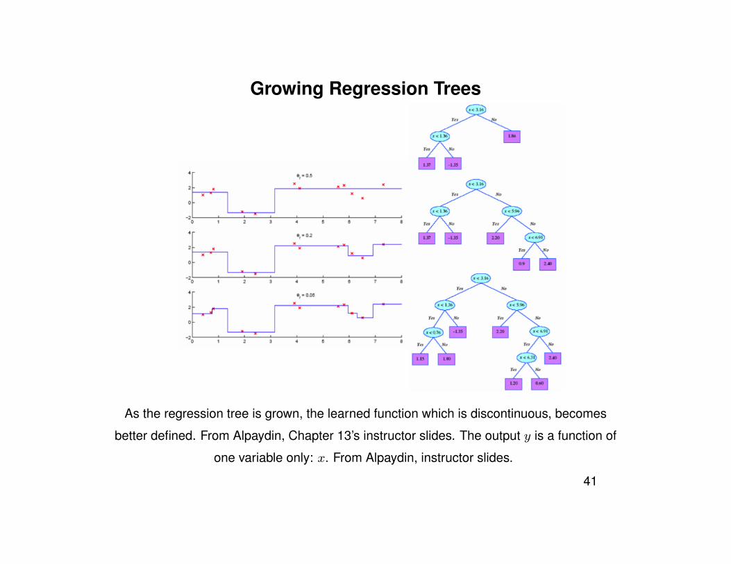
Growing Regression Trees

As the regression tree is grown, the learned function which is discontinuous, becomes

better defined. From Alpaydin, Chapter 13’s instructor slides. The output y is a function of

one variable only: x. From Alpaydin, instructor slides.

41

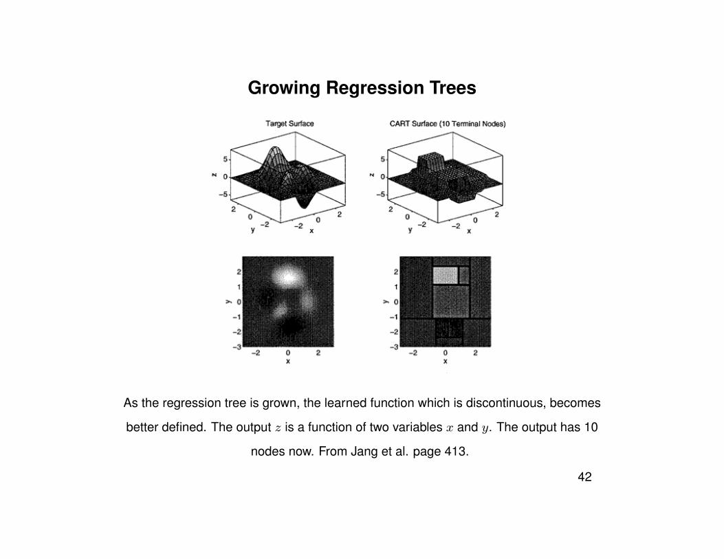
Growing Regression Trees

As the regression tree is grown, the learned function which is discontinuous, becomes

better defined. The output z is a function of two variables x and y. The output has 10

nodes now. From Jang et al. page 413.

42

Growing Regression Trees

As the regression tree is grown, the learned function which is discontinuous, becomes

better defined. The output z is a function of two variables x and y. The tree has 20 nodes

now. From Jang et al. page 414.

43

Pruning Regression Trees

• A regression tree is grown to an overfitted size just like adecision tree.

• The tree is then pruned. First prune any node whose re-moval doesn’t reduce performance of the tree on a test orvalidation set. Rearrange the tree if necessary. Repeat thepruning process till the tree’s performance doesn’t deterio-rate.

• As a tree is pruned, the output regression function becomesless smooth (opposite of what we see in the regression treegrowing examples).

44

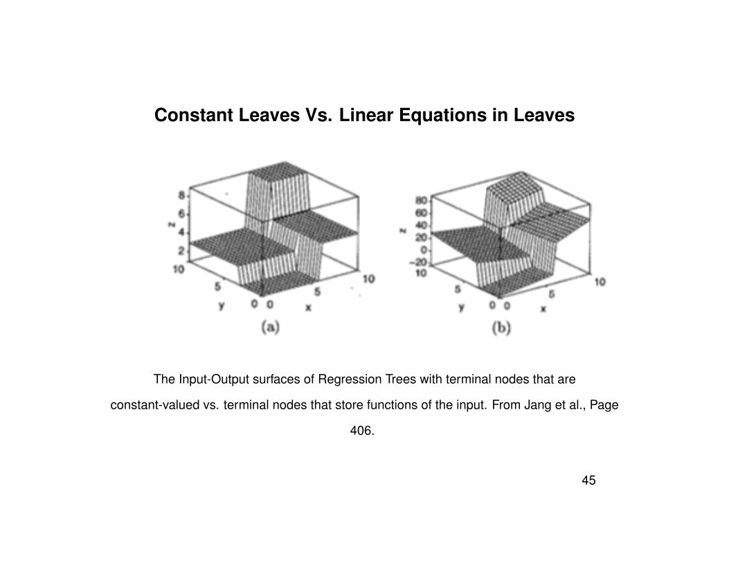
Constant Leaves Vs. Linear Equations in Leaves

The Input-Output surfaces of Regression Trees with terminal nodes that are

constant-valued vs. terminal nodes that store functions of the input. From Jang et al., Page

406.

45

Mutlivariate Decision/Regression Trees

• A node can have a condition composed of more than onefeature in linear or non-linear combination. From Alpaydin,instructor slides.

• Having very complex conditions defeats the one purpose ofbuilding a decision tree which is creating classification rulesthat can be explained.

46

Omnivariate Decision/Regression Trees

• An omnivariate tree allows both univariate or multivariatenodes, both linear and non-linear.

• Different types of nodes are compared with statistical testsand the best one chosen.

• A simpler node is chosen unless a complex one gives muchbetter accuracy.

• Usually more complex nodes occur near root when we havemore data and simpler nodes occur near leaves when wehave less data to work with.

47

Balancing subtrees

• Many machine learning algorithms do not perform well if thetraining data is unbalanced in class sizes.

• However, in real life, unbalanced classes are common. Oneneeds a way not to be biased by the bigger classes.

• The CART program uses some techniques to keep the classesbalanced as much as possible.

48