"Decessit sine prole" Childlessness, Celibacy, and Survival of the Richest in Pre-Industrial England

D. de la Croix, E.B. Schneider and J. Weisdorf

Discussion Paper 2017-1

“Decessit sine prole” –Childlessness, Celibacy, and Survival of the Richest

in Pre-Industrial England

David de la Croix1 Eric B. Schneider2 Jacob Weisdorf3

January 5, 2017

Abstract

Previous work has shown that England’s pre-industrial elites had more surviving off-spring than their lower-class counterparts. This evidence was used to argue that the spreadof upper-class values via downward social mobility helped England grow rich. We contestthis view, showing that the lower classes outperformed the rich in terms of reproductiononce singleness and childlessness are accounted for. Indeed, Merchants, Professionals andGentry married less, and their marriages were more often childless. Many died without de-scendants (decessit sine prole). We also establish that the most prosperous socio-economicgroup in terms of reproduction was the middle class, which we argue was instrumental toEngland’s economic success because most of its new industrialists originated from middle-class families.

1IRES and CORE, UCLouvain. Email: david.delacroix@uclouvain.be.2London School of Economics and CEPR. Email: e.b.schneider@lse.ac.uk.3University of Southern Denmark and CEPR. Email: jacobw@sam.sdu.dk.

Acknowledgements: David de la Croix acknowledges the financial support of the project ARC 15/19-063 ofthe Belgian French speaking Community. We thank Gregory Clark, Neil Cummins, and participants to theworkshop on “The importance of Elites and their demography for Knowledge and Development” (UCLouvain,2016) for comments on an earlier draft.

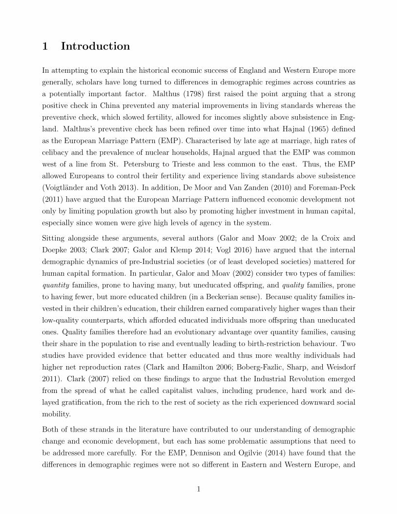
1 Introduction

In attempting to explain the historical economic success of England and Western Europe more

generally, scholars have long turned to differences in demographic regimes across countries as

a potentially important factor. Malthus (1798) first raised the point arguing that a strong

positive check in China prevented any material improvements in living standards whereas the

preventive check, which slowed fertility, allowed for incomes slightly above subsistence in Eng-

land. Malthus’s preventive check has been refined over time into what Hajnal (1965) defined

as the European Marriage Pattern (EMP). Characterised by late age at marriage, high rates of

celibacy and the prevalence of nuclear households, Hajnal argued that the EMP was common

west of a line from St. Petersburg to Trieste and less common to the east. Thus, the EMP

allowed Europeans to control their fertility and experience living standards above subsistence

(Voigtlander and Voth 2013). In addition, De Moor and Van Zanden (2010) and Foreman-Peck

(2011) have argued that the European Marriage Pattern influenced economic development not

only by limiting population growth but also by promoting higher investment in human capital,

especially since women were give high levels of agency in the system.

Sitting alongside these arguments, several authors (Galor and Moav 2002; de la Croix and

Doepke 2003; Clark 2007; Galor and Klemp 2014; Vogl 2016) have argued that the internal

demographic dynamics of pre-Industrial societies (or of least developed societies) mattered for

human capital formation. In particular, Galor and Moav (2002) consider two types of families:

quantity families, prone to having many, but uneducated offspring, and quality families, prone

to having fewer, but more educated children (in a Beckerian sense). Because quality families in-

vested in their children’s education, their children earned comparatively higher wages than their

low-quality counterparts, which afforded educated individuals more offspring than uneducated

ones. Quality families therefore had an evolutionary advantage over quantity families, causing

their share in the population to rise and eventually leading to birth-restriction behaviour. Two

studies have provided evidence that better educated and thus more wealthy individuals had

higher net reproduction rates (Clark and Hamilton 2006; Boberg-Fazlic, Sharp, and Weisdorf

2011). Clark (2007) relied on these findings to argue that the Industrial Revolution emerged

from the spread of what he called capitalist values, including prudence, hard work and de-

layed gratification, from the rich to the rest of society as the rich experienced downward social

mobility.

Both of these strands in the literature have contributed to our understanding of demographic

change and economic development, but each has some problematic assumptions that need to

be addressed more carefully. For the EMP, Dennison and Ogilvie (2014) have found that the

differences in demographic regimes were not so different in Eastern and Western Europe, and

1

all studies of the EMP tend to assume a homogenous demographic regime within a country. At

the same time, the survival of the richest literature has not properly accounted for differential

rates of celibacy and childlessness across classes when computing the reproductive success of

each group (Boberg-Fazlic, Sharp, and Weisdorf 2011).

This paper addresses these earlier shortcomings by analysing the internal fertility dynamics of

pre-Industrial England. We use the family reconstitution data collected from English parish

registers and assembled by the Cambridge Group (Wrigley et al. 1997) to estimate the reproduc-

tive success of different wealth groups. Compared to previous attempts to measure reproductive

success in historical England, which calculate reproductive rates conditional on giving birth,

our study considers both the intensive margin, i.e. an individual’s number of surviving off-

spring, and the extensive margin, i.e. whether or not an individual married or had children at

all (Aaronson, Lange, and Mazumder 2014 and Baudin, de la Croix, and Gobbi 2015). Thus,

we explore reproductive success across four margins: two extensive margins - the choice to

marry and the choice to have children - and two intensive margins - the number of children

born and the child death rate. By accounting for the four margins of reproduction we are able

to map out class-specific historical demography in England. Our findings dispute the previous

view that the upper classes had more surviving offspring than the lower classes. We show that

the middle classes were the most successful socio-economic group in terms of reproduction once

taking account of the extensive margin of fertility. Merchants, professionals and gentry, the

upper classes, had high rates of celibacy and childlessness driving down their overall reproduc-

tive success, whereas labourers, servants and husbandmen had much lower rates of celibacy and

childlessness but limited their fertility within marriage likely through birth spacing. Thus, the

middle classes combined high fertility and low celibacy and childlessness and therefore had the

highest net reproduction rates.

We argue that this demographic regime provides a more intuitive explanation for historical Eng-

land’s economic success than those put forth in the previous work highlighted above. Middle

class families were more likely to invest in apprenticeships for their children (Minns and Wallis

2012) and according to Crouzet (1985) more than 85 per cent of England’s early industrialists

came from a middle-class background. This practical education led to a build-up of upper-tail

human capital that Mokyr (2005) argued and Squicciarini and Voigtlander (2015) found was

more important for industrialisation than general levels of literacy. Thus, the reproductive ad-

vantage of middle class English families in the pre-Industrial era helped to create preconditions

necessary for the Industrial Revolution.

Our findings also challenge simple models of the EMP that treat countries as internally homoge-

nous. We show that demographic behaviour varied substantially by class and that different

groups in society used different forms of fertility limitation. This raises questions about the

2

dynamic processes underlying the EMP. For example, if celibacy were more common among

the wealthy, then celibacy is unlikely to have been responsive to economic conditions in the

way that Malthus (1798) and Voigtlander and Voth (2013) thought. Thus, more dynamic and

flexible models of the EMP need to be developed to better understand this important historical

institution.

The paper unfolds as follows. Section 2 illustrates the different margins through which social

status affects reproduction and reviews the literature on celibacy, childlessness and the Euro-

pean Marriage Pattern. Section 3 describes the data used for the analysis and how we define

social classes. In Section 4 we calculate the class-specific rates of celibacy, childlessness, marital

fertility and child mortality and translate these rates into class-specific net rates of reproduc-

tion. Section 5 argues that our results are not driven by selective migration. Finally, section 6

discusses the implications of the results and Section 7 concludes.

2 Theoretical and Historiographical Underpinnings

Before proceeding to the analysis, it is first necessary to describe the theoretical and histori-

ographical underpinnings of our study. We first provide a theoretical approach to calculating

the four margins of fertility. Then we provide a brief summary of celibacy, childlessness and

the EMP explaining how our study intervenes in the existing literature.

2.1 Theory

As mentioned above, our paper considers two neglected aspects of overall fertility: celibacy

and childlessness. We present differences in the four margins of fertility by social group using

the following framework (extending the approach in Baudin, de la Croix, and Gobbi (2016)).

Households are heterogenous by social class c. We consider two types of marital status: married

and singles. The marriage rate depends on c: m(c). We assume singles do not have children.

Net reproduction n(·) as a function of social class c is:

n(c) = m(c) (1− z(c)) b(c) (1− d(c)) (1)

where z(c) is the fraction of childless married women, b(c) is the number of births conditional

on being married and having children, and d(c) is the mortality rate of children aged 0 to

15. Usually, the literature finds that in pre-industrial societies the social gradient of births is

positive (Skirbekk et al. 2008), b′(c) ≥ 0, and the social gradient in mortality is negative or

nil, d′(c) ≤ 0, i.e. wealthier households have larger families and experience lower rates of child

3

mortality.

In most of the literature, one considers marital fertility, implying that the marriage margin is

constant (Wrigley et al. 1997, p. 428), and in some cases the extensive margin of fertility is

constant too (Boberg-Fazlic, Sharp, and Weisdorf 2011), m(c) = m and z(c) = z, implying that

the effect of social class on fertility is positive,

n′(c) = m(1− z) ((1− d(c))b′(c)− b(c)d′(c)) > 0,

as b′(c) ≥ 0 and d′(c) < 0.

In general though, the effect of social class on reproduction n is the sum of four effects:

n′(c) = (1− z(c))b(c)(1− d(c)) m′(c)︸ ︷︷ ︸marriage margin

−m(c)b(c)(1− d(c)) z′(c)︸ ︷︷ ︸childlessness margin︸ ︷︷ ︸

Extensive margins of fertility

+ m(c)(1− z(c)) ((1− d(c)) b′(c) − b(c) d′(c))︸ ︷︷ ︸intensive margin of fertility

.

If marriage rates decrease with social class and/or childlessness rates increase with social class,

it is possible that the rich would not be so reproductively successful after all. Formally, this

happens when

b(c)(1− d(c))(m(c)z′(c)− (1− z(c))m′(c) > m(c)(1− z(c))((1− d(c))b′(c)− b(c)d′(c)). (2)

If marriage rates and/or childlessness rates are non-monotonic functions of social class, the

pattern of reproductive success can become more complicated. To know whether condition (2)

holds in reality, one needs to estimate z(c), m(c), b(c) and d(c) from data.

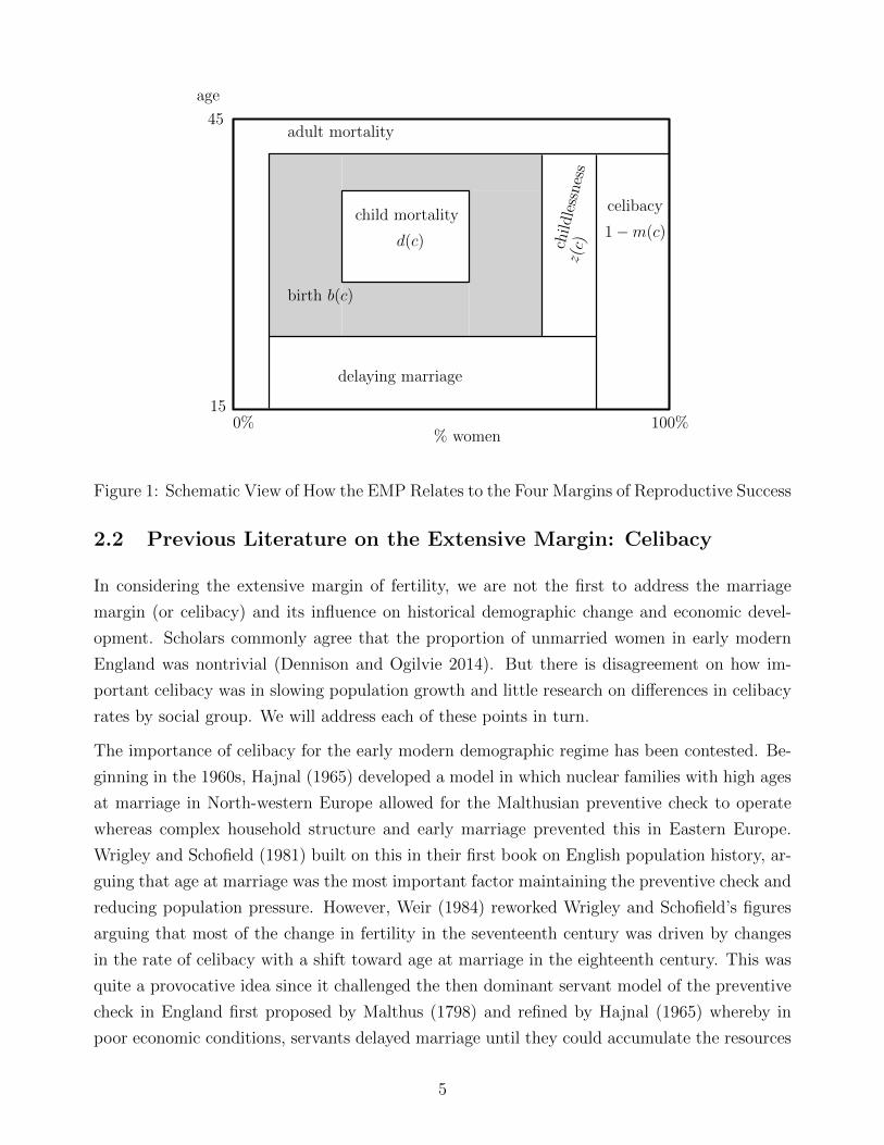
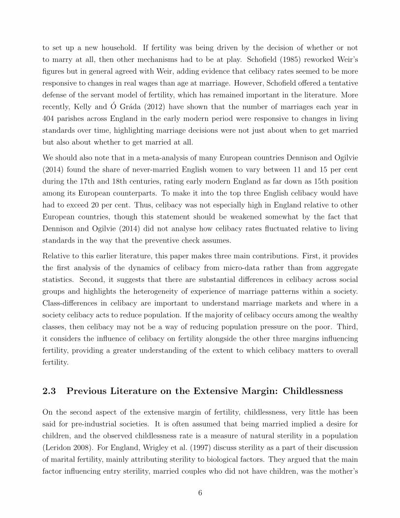
The relation between our decomposition (1) and the so-called European Marriage Pattern

(EMP) is explained in Figure 1. The bigger rectangle represents the maximum reproduction

obtained when 100 per cent of women (horizontal axis) marry at age 15 (vertical axis). The

usual representation of the European Marriage Pattern argues that by delaying marriage and

having some dose of celibacy, the span of reproduction is reduced. In this paper, we consider the

vertical line 1−m(c) as dependent on social class. We add a second vertical line, representing

childless couples. Taking into account child mortality, represented by the inner rectangle, we

are left with the grey area representing reproduction. Thus, our paper calculates the size of the

shaded box for different social groups to understand the social gradient in reproductive success.

4

age

45

15

% women0% 100%

child mortality

delaying marriage

celibacy

childlessness

birth b(c)

d(c)

z(c)

1−m(c)

adult mortality

Figure 1: Schematic View of How the EMP Relates to the Four Margins of Reproductive Success

2.2 Previous Literature on the Extensive Margin: Celibacy

In considering the extensive margin of fertility, we are not the first to address the marriage

margin (or celibacy) and its influence on historical demographic change and economic devel-

opment. Scholars commonly agree that the proportion of unmarried women in early modern

England was nontrivial (Dennison and Ogilvie 2014). But there is disagreement on how im-

portant celibacy was in slowing population growth and little research on differences in celibacy

rates by social group. We will address each of these points in turn.

The importance of celibacy for the early modern demographic regime has been contested. Be-

ginning in the 1960s, Hajnal (1965) developed a model in which nuclear families with high ages

at marriage in North-western Europe allowed for the Malthusian preventive check to operate

whereas complex household structure and early marriage prevented this in Eastern Europe.

Wrigley and Schofield (1981) built on this in their first book on English population history, ar-

guing that age at marriage was the most important factor maintaining the preventive check and

reducing population pressure. However, Weir (1984) reworked Wrigley and Schofield’s figures

arguing that most of the change in fertility in the seventeenth century was driven by changes

in the rate of celibacy with a shift toward age at marriage in the eighteenth century. This was

quite a provocative idea since it challenged the then dominant servant model of the preventive

check in England first proposed by Malthus (1798) and refined by Hajnal (1965) whereby in

poor economic conditions, servants delayed marriage until they could accumulate the resources

5

to set up a new household. If fertility was being driven by the decision of whether or not

to marry at all, then other mechanisms had to be at play. Schofield (1985) reworked Weir’s

figures but in general agreed with Weir, adding evidence that celibacy rates seemed to be more

responsive to changes in real wages than age at marriage. However, Schofield offered a tentative

defense of the servant model of fertility, which has remained important in the literature. More

recently, Kelly and O Grada (2012) have shown that the number of marriages each year in

404 parishes across England in the early modern period were responsive to changes in living

standards over time, highlighting marriage decisions were not just about when to get married

but also about whether to get married at all.

We should also note that in a meta-analysis of many European countries Dennison and Ogilvie

(2014) found the share of never-married English women to vary between 11 and 15 per cent

during the 17th and 18th centuries, rating early modern England as far down as 15th position

among its European counterparts. To make it into the top three English celibacy would have

had to exceed 20 per cent. Thus, celibacy was not especially high in England relative to other

European countries, though this statement should be weakened somewhat by the fact that

Dennison and Ogilvie (2014) did not analyse how celibacy rates fluctuated relative to living

standards in the way that the preventive check assumes.

Relative to this earlier literature, this paper makes three main contributions. First, it provides

the first analysis of the dynamics of celibacy from micro-data rather than from aggregate

statistics. Second, it suggests that there are substantial differences in celibacy across social

groups and highlights the heterogeneity of experience of marriage patterns within a society.

Class-differences in celibacy are important to understand marriage markets and where in a

society celibacy acts to reduce population. If the majority of celibacy occurs among the wealthy

classes, then celibacy may not be a way of reducing population pressure on the poor. Third,

it considers the influence of celibacy on fertility alongside the other three margins influencing

fertility, providing a greater understanding of the extent to which celibacy matters to overall

fertility.

2.3 Previous Literature on the Extensive Margin: Childlessness

On the second aspect of the extensive margin of fertility, childlessness, very little has been

said for pre-industrial societies. It is often assumed that being married implied a desire for

children, and the observed childlessness rate is a measure of natural sterility in a population

(Leridon 2008). For England, Wrigley et al. (1997) discuss sterility as a part of their discussion

of marital fertility, mainly attributing sterility to biological factors. They argued that the main

factor influencing entry sterility, married couples who did not have children, was the mother’s

6

age at marriage since only 2.6 and 3.8 per cent of women who married at ages 15-19 or 20-24

respectively never bore children whereas 69.3 per cent of women who were first married at the

age of 40-44 never bore children. Across all ages entry sterility varied between 8.3 and 11.5

per cent across the early modern period generally following overall trends in fertility (p. 403).

Hollingsworth (1965), who studied the demographics of British nobles based on genealogical

records, finds an average rate of childlessness at 24 per cent, based on all persons ever married,

a surprisingly high rate compared with other populations and the average entry sterility rates

for English provincial parishes (Wrigley et al. 1997, pp. 395-397).

In France, scholars have explored childlessness and sterility by social class more directly. Bardet

(1983), who reconstituted 5889 complete family histories over the seventeenth and eighteenth

centuries, shows a table (p. 300) with the percentage of childless women by year at marriage

and social class. The childlessness rate is computed based on women who married before 30

years old, and for whom we have a complete record of life events. The social gradient was

positive, i.e. childlessness was more widespread among nobles and shopkeepers than among

workers, and there was a positive time trend in the data. On the whole, Bardet’s figures are

above the natural sterility rate estimated elsewhere (Leridon 2008).

Beyond biological factors, there might also be economic determinants of childlessness. Three

recent papers stress those determinants for US data in a historical perspective. Gobbi (2013)

shows how childlessness rates and fertility rates co-move over time as a function of shocks to the

gender gap and to the cost of having children. Aaronson, Lange, and Mazumder (2014) focus

on a quantity-quality trade-off faced by parents and look at how the Rosenwald Rural Schools

Initiative in the early twentieth century affected fertility along both the extensive and intensive

margins. They show that the expansion of schooling opportunities decreased the price of child

quality. This reduction in the price of child quality decreased the proportion of women with

the highest fertility rates as expected, but it also led to a decrease in childlessness rates as more

women entered on the extensive margin. In addition, Baudin, de la Croix, and Gobbi (2015)

provide a framework to understand the deep causes of childlessness and how their importance

has changed over time. Using US census data, they find that the main causes of childlessness

across the past 100 years have changed from poverty-induced necessity to a choice driven by

higher levels of income and education among women.

By treating the childlessness margin separately, we also contribute to this literature providing

figures for England similar to Bardet (1983). We also find evidence that childlessness was

not entirely involuntary since there were significant class differences in childlessness of women

within marriage. This finding contributes to the erosion of the simple version of the Malthusian

preventive check based solely on celibacy and age at marriage.

7

2.4 The European Marriage Pattern

Finally, linking the extensive and intensive margins together is one of the strongest models

for how economic behaviour influenced economic development in the pre-Industrial era: the

European Marriage Pattern (EMP). This pattern of high rates of celibacy, late ages of mar-

riage and the formation of new, nuclear households at marriage was first described by Hajnal

(1965) and has been expanded since then. There are two explanations of the origins of the

EMP. De Moor and Van Zanden (2010) argue that norms of consent among marriage partners

which emerged in Catholic doctrine in the ninth century led to more respect for and empow-

erment of women, producing the EMP, whereas Voigtlander and Voth (2013) argue that the

population shock of the Black Death and women’s comparative advantage in the pastoral sec-

tor improved women’s labour market opportunities and led to later marriage. In the more

traditional argument, the EMP influenced economic development by reducing fertility and pre-

venting population growth from capturing all of the growth achieved through improvements in

technology or extensive expansion in the area under agriculture (Voigtlander and Voth 2013).

However, more recent studies have also highlighted the important benefits that the EMP had

on human capital formation. Since family income was above subsistence, more resources could

be invested in acquiring knowledge and skills. In addition, by giving women time to acquire

formal and informal skills before childbearing, women were able to gain further agency and eco-

nomic power. Women’s labour participation and the formation of human capital helped keep

wages high and rising and eventually produced further economic success (De Moor and Van

Zanden 2010; Foreman-Peck 2011). Carmichael et al. (2016) have highlighted that the success

of the EMP relied on non-demographic factors as well such as consensus surrounding marriage

and neo-locality in household formation: newly married couples formed their own household

directly after marriage.

However, this schematic and somewhat simplified view of the EMP in England has recently

been challenged on a number of fronts. First, Dennison and Ogilvie (2014) have conducted a

meta-analysis of the demographic characteristics of a number of European countries on both

sides of Hajnal’s line. They collected systematic information on female age at first marriage,

celibacy rates and household complexity and found no correlation between key elements of

Hajnal’s European Marriage Pattern and economic development. In addition, two other papers

have shown that people living in early modern England may have had a larger degree of fertility

control than had been assumed, a fundamental breach of the traditional Malthusian population

model. Kelly and O Grada (2012), studying counts of births in 404 English parishes, found

evidence that births responded to economic conditions in early modern England with parishes

having fewer births when economic conditions were bad. Cinnirella, Klemp, and Weisdorf

8

(2017) also found that the risk of having a child was lower when conditions were bad analysing

the individual-level family reconstitution data employed in this paper. If families were able to

limit their fertility within marriage, then the rates of celibacy and age at marriage might have

been less important than the proponents of the EMP have thought.

Our contribution to this literature is to analyse the workings of the EMP within wealth groups

of one country to give an idea of how the EMP was practiced within pre-Industrial English

society. This analysis will reveal the extent to which the EMP factors were heterogeneous

across groups.

3 Database

3.1 Data Quality

Having presented the theoretical and historical background, we now turn to the data. We use

the family reconstitution data collected by the Cambridge Group for the History of Population

and Social Structure and described in detail by Wrigley et al. (1997). The full dataset includes

over 300,000 individuals recorded in registers coming from a total of 26 provincial, English

parishes. The data are drawn from baptism, marriage and burial registers kept by the local

parish priest, which have been systematically linked so that individuals can be tracked across

their lifetime from birth, to marriage, to the birth (and potentially burial) of their children, to

their own burial (Wrigley 1966). In addition to the demographic events present in the registers,

male occupations were often recorded upon a man’s marriage or burial or when his child was

baptised. It is from these occupations that we construct our social groups.

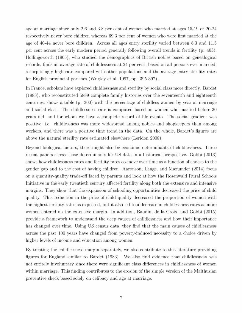
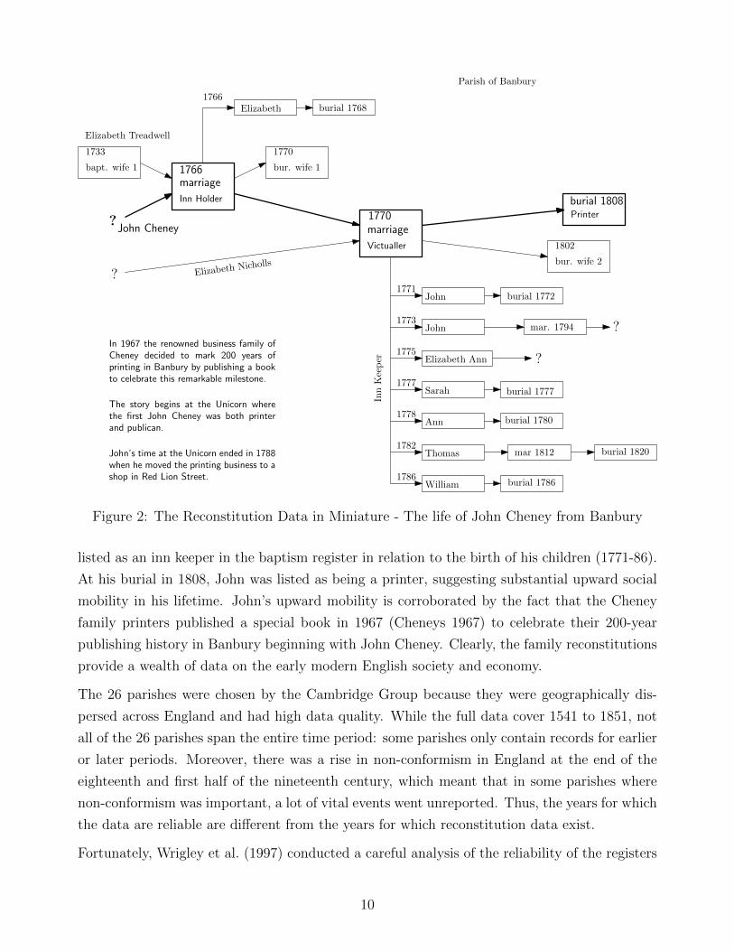
To provide an idea of how the reconstitution data work, Figure 2 shows the example of John

Cheney from the parish of Banbury. John was born outside the parish, so we do not observe

his birth date in the baptism register. He appears in our dataset when he marries Elizabeth

Treadwell in Banbury in 1766. Unfortunately, Elizabeth and their only child died by 1770,

so in the same year, John married Elizabeth Nicholls, with whom he went on to have seven

children. Among the children from his second marriage, four died within two years of birth.

The youngest child, Thomas, married and died at age 38 in the parish. We assume Elizabeth

Ann migrated out of the parish since we do not observe her marriage or burial. Finally, John’s

son John (the surviving one) married in the parish and then migrated since we do not observe

his burial. John’s second wife died in 1802, and he passed away in 1808. We can also track John

(the father)’s occupation over time. His occupation is initially recorded at his first marriage

as inn holder. Then, by his second marriage in 1770 he has become a victualler, though he is

9

1733

bapt. wife 1 1766marriage

Inn Holder

1770

bur. wife 1

1766Elizabeth burial 1768

1770marriage

Victualler

burial 1808Printer

1802

bur. wife 2

1771

1773

1775

1777

1778

1782

1786

John

John

Elizabeth Ann

Sarah

Ann

Thomas

William

?

?

?

?

burial 1772

mar. 1794

burial 1777

burial 1780

mar 1812 burial 1820

burial 1786

InnKeeper

ElizabethNicholls

Elizabeth Treadwell

John Cheney

Parish of Banbury

In 1967 the renowned business family ofCheney decided to mark 200 years ofprinting in Banbury by publishing a bookto celebrate this remarkable milestone.

The story begins at the Unicorn wherethe first John Cheney was both printerand publican.

John’s time at the Unicorn ended in 1788when he moved the printing business to ashop in Red Lion Street.

Figure 2: The Reconstitution Data in Miniature - The life of John Cheney from Banbury

listed as an inn keeper in the baptism register in relation to the birth of his children (1771-86).

At his burial in 1808, John was listed as being a printer, suggesting substantial upward social

mobility in his lifetime. John’s upward mobility is corroborated by the fact that the Cheney

family printers published a special book in 1967 (Cheneys 1967) to celebrate their 200-year

publishing history in Banbury beginning with John Cheney. Clearly, the family reconstitutions

provide a wealth of data on the early modern English society and economy.

The 26 parishes were chosen by the Cambridge Group because they were geographically dis-

persed across England and had high data quality. While the full data cover 1541 to 1851, not

all of the 26 parishes span the entire time period: some parishes only contain records for earlier

or later periods. Moreover, there was a rise in non-conformism in England at the end of the

eighteenth and first half of the nineteenth century, which meant that in some parishes where

non-conformism was important, a lot of vital events went unreported. Thus, the years for which

the data are reliable are different from the years for which reconstitution data exist.

Fortunately, Wrigley et al. (1997) conducted a careful analysis of the reliability of the registers

10

and report the corresponding dates for each parish (p. 22-23). We accordingly introduce our

own censoring dates at the reliable start and stop year for each parish. However, we could choose

to be more or less dogmatic about this. On the more dogmatic side, we could require all of the

births, marriages and deaths that we count to be within the reliable dates for the data, reducing

our sample size substantially. On the less dogmatic side, which we will adopt, we could require

the marriage date to be 15 years before the end of the reliable period. This strategy ensures

that we observe nearly all of a woman’s potential children, but we would not lose observations

because we did not observe the mother’s death date until after the records became less reliable.

This way of censoring the data may lead to slight problems with the absolute level of fertility

that we predict but would not influence the relative fertility of different groups. The censoring

leads to a loss of individual observations of 21.6 per cent.

3.2 Social Groups

In order to measure the four margins of fertility across a social gradient, we must first sort

occupations in our dataset into meaningful social groups. There are a number of ways that

we could sort the occupations, including by HISCLASS (Van Leeuwen and Maas 2011) or the

nineteenth-century British professional groups (Armstrong, 1972, Long, 2013), but we have

opted to follow the previous literature and use Clark and Hamilton (2006)’s wealth categories

which were also employed by Boberg-Fazlic, Sharp, and Weisdorf (2011) and Clark and Cum-

mins (2015). These reflect occupations that were frequently recorded in wills by wealth and

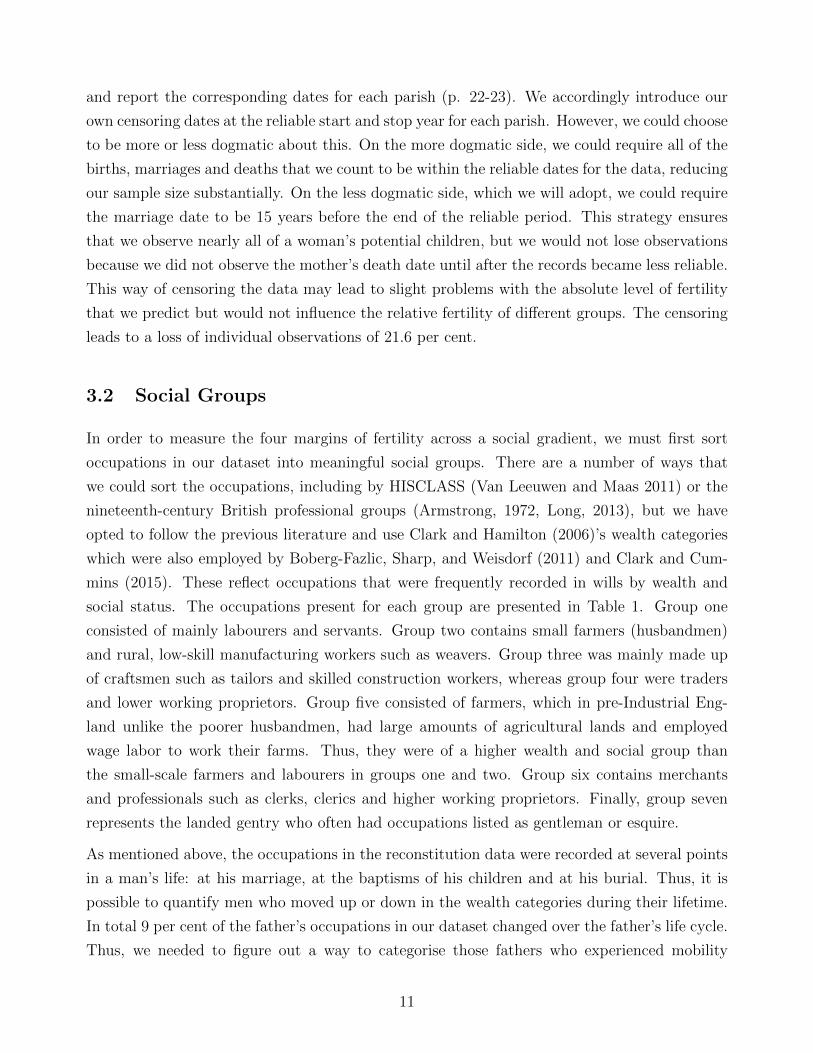
social status. The occupations present for each group are presented in Table 1. Group one

consisted of mainly labourers and servants. Group two contains small farmers (husbandmen)

and rural, low-skill manufacturing workers such as weavers. Group three was mainly made up

of craftsmen such as tailors and skilled construction workers, whereas group four were traders

and lower working proprietors. Group five consisted of farmers, which in pre-Industrial Eng-

land unlike the poorer husbandmen, had large amounts of agricultural lands and employed

wage labor to work their farms. Thus, they were of a higher wealth and social group than

the small-scale farmers and labourers in groups one and two. Group six contains merchants

and professionals such as clerks, clerics and higher working proprietors. Finally, group seven

represents the landed gentry who often had occupations listed as gentleman or esquire.

As mentioned above, the occupations in the reconstitution data were recorded at several points

in a man’s life: at his marriage, at the baptisms of his children and at his burial. Thus, it is

possible to quantify men who moved up or down in the wealth categories during their lifetime.

In total 9 per cent of the father’s occupations in our dataset changed over the father’s life cycle.

Thus, we needed to figure out a way to categorise those fathers who experienced mobility

11

1 Labourers/Servants incl. seamen

2 Husbandmen small farmers, weavers

3 Craftsmen tailors, carpenters

4 Traders innkeepers, butchers, bakers

5 Farmers

6 Merchants/Professionals clerks, medical

7 Gentry gentlemen, esquire

Table 1: Social Groups Employed in the Analysis

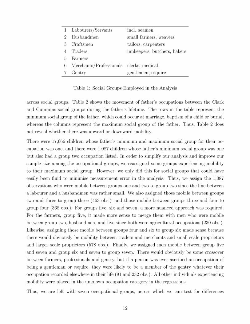
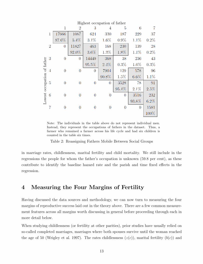
across social groups. Table 2 shows the movement of father’s occupations between the Clark

and Cummins social groups during the father’s lifetime. The rows in the table represent the

minimum social group of the father, which could occur at marriage, baptism of a child or burial,

whereas the columns represent the maximum social group of the father. Thus, Table 2 does

not reveal whether there was upward or downward mobility.

There were 17,666 children whose father’s minimum and maximum social group for their oc-

cupation was one, and there were 1,087 children whose father’s minimum social group was one

but also had a group two occupation listed. In order to simplify our analysis and improve our

sample size among the occupational groups, we reassigned some groups experiencing mobility

to their maximum social group. However, we only did this for social groups that could have

easily been fluid to minimise measurement error in the analysis. Thus, we assign the 1,087

observations who were mobile between groups one and two to group two since the line between

a labourer and a husbandmen was rather small. We also assigned those mobile between groups

two and three to group three (463 obs.) and those mobile between groups three and four to

group four (368 obs.). For groups five, six and seven, a more nuanced approach was required.

For the farmers, group five, it made more sense to merge them with men who were mobile

between group two, husbandmen, and five since both were agricultural occupations (230 obs.).

Likewise, assigning those mobile between groups four and six to group six made sense because

there would obviously be mobility between traders and merchants and small scale proprietors

and larger scale proprietors (578 obs.). Finally, we assigned men mobile between group five

and seven and group six and seven to group seven. There would obviously be some crossover

between farmers, professionals and gentry, but if a person was ever ascribed an occupation of

being a gentleman or esquire, they were likely to be a member of the gentry whatever their

occupation recorded elsewhere in their life (91 and 232 obs.). All other individuals experiencing

mobility were placed in the unknown occupation category in the regressions.

Thus, we are left with seven occupational groups, across which we can test for differences

12

Highest occupation of father

Low

est

occ

upat

ion

offa

ther

Note: The individuals in the table above do not represent individual men.Instead, they represent the occupations of fathers in the dataset. Thus, afarmer who remained a farmer across his life cycle and had six children iscounted in the table six times.

Table 2: Reassigning Fathers Mobile Between Social Groups

in marriage rates, childlessness, marital fertility and child mortality. We still include in the

regressions the people for whom the father’s occupation is unknown (59.8 per cent), as these

contribute to identify the baseline hazard rate and the parish and time fixed effects in the

regression.

4 Measuring the Four Margins of Fertility

Having discussed the data sources and methodology, we can now turn to measuring the four

margins of reproductive success laid out in the theory above. There are a few common measure-

ment features across all margins worth discussing in general before proceeding through each in

more detail below.

When studying childlessness (or fertility at other parities), prior studies have usually relied on

so-called completed marriages, marriages where both spouses survive until the woman reached

the age of 50 (Wrigley et al. 1997). The rates childlessness (z(c)), marital fertility (b(c)) and

13

child mortality (d(c)) can then be estimated using a sample of women who reached the end

of their reproductive period, say aged 50+. However, as we are interested in the reproductive

success of different social groups, we should not neglect the contribution of women who died

prematurely, i.e. before age 50, to reproduction. Although these women will have fewer children

than those with completed fertility, their children still contribute to reproductive success. We

therefore use Cox Proportional Hazard models for censored data to estimate the four margins,

m(c), z(c), b(c) and d(c). As regressors we use the seven occupational dummies defined above

plus a dummy for individuals of unknown occupation, and we control for parish and time fixed

effects by including twenty-six parish dummies and four time dummies (one for each quartile

of the data ranked by year of marriage: 1538-1649, 1650-1718, 1719-1769, 1769-1836) in the

regressions. The reference category is a Labourer/Servant married in 1650-1718 in the parish of

Alcester. Although previous studies have split the data into various periods, we are reluctant

to do this because it would reduce our sample size for some of the estimations to a very low

level and exacerbate compositional effects of parishes and the small number of individuals in

certain groups. This section describes the subset of data that corresponds to each calculation,

discusses how each of the components is estimated and analyses the difference across social

groups in each of the four margins.

4.1 Marriage Rate m(c)

Although family reconstitution data, which are centred around marriages, may seem at first to

be less than ideal for analysing people who never married, we can study lifetime celibacy by

analysing the life courses of the children from each marriage. By looking at cohorts of births,

we are able to compute the share of unmarried individuals by their age of death, providing a

full picture of celibacy across the entire lifecycle.

Rather than following the literature so far by measuring celibacy among women surviving past

a certain age (say 40 or 50), we use Cox proportional hazard models to measure the risk

of marriage across the life course. This method will produce higher rates of celibacy than

other studies because we account for women who married and/or died before the cut off age.

Women’s risk of marriage begins when they turn 16, the age at which women were allowed

to marry according to Anglican tradition, and was only censored at the upper end when the

woman died. Thus, we exclude women who died below the age of 16 and were never at risk of

marriage.

To compute our indicator of celibacy, we take the predicted marriage rate from the survival

curves at the age of 45, which is m(c). We choose age 45 because very few marriages occurred

after age 45 and very few women were able to have children after the age of 45, so marriages

14

beyond 45 were unlikely to influence net fertility across social groups. In addition, we impose

the following requirements on the data to construct the sample used to predict the survival

curves: we count women in the data as married if they (i) were baptised and buried in the

sampled parish; (ii) survived beyond the age of 16 as mentioned above; and (iii) were registered

as being married or having baptised a child in the parish. Lifetime celibate women satisfied

conditions (i) and (ii) but were not registered as married or baptising children in the parish.

The first condition is necessary because it restricts the sample to individuals who were born in

the parish and never migrated permanently. This is especially important for observing lifetime

celibate women because if an individual came from an unobserved parish (i.e. has a missing

baptism date) or moved to an unobserved parish (i.e. has a missing burial date), we cannot be

sure that she did not get married in an unobserved parish either before entering or after leaving

the observed parish.

Table A.8 in Appendix A provides information on the sample of women for whom we calculate

the marriage rate. There are a total of 8,611 women satisfying (i) and (ii), and 58.6 per cent

of them are registered as married, hence satisfying (i), (ii), and (iii).

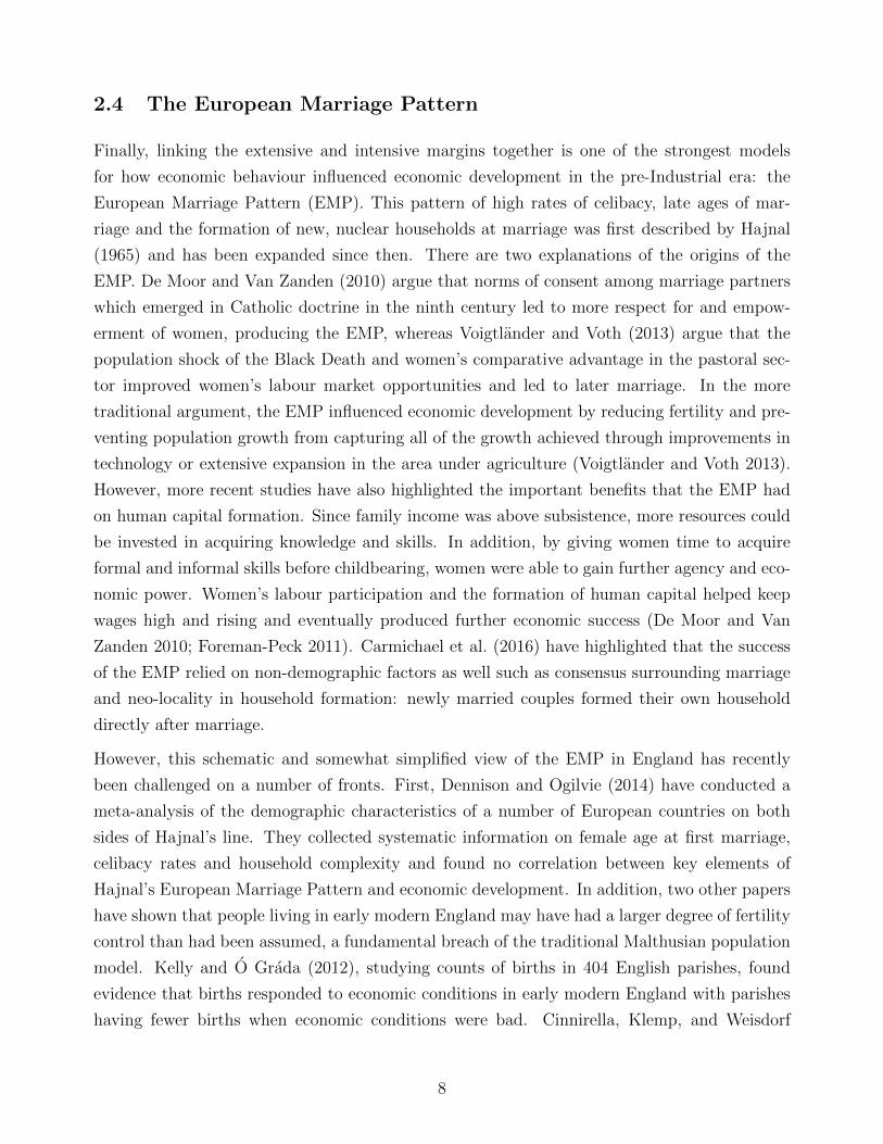
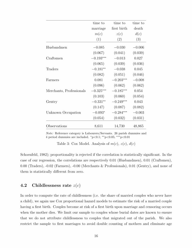
Column (1) in Table 3 shows the results from the Cox proportional hazard model estimating

the risk of marriage. Daughters of merchants/professionals and gentry had substantially lower

risks of marriage, but daughters of craftsmen, traders and the unknown occupations were also

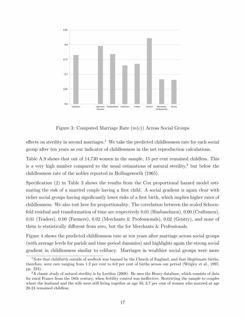
less likely to marry than the reference category, daughters of laborers and servants. Figure 3

shows the marriage rate across the social groups predicted from the survival curve from the Cox

model at age 45 with average levels imputed for all parish and time dummies. As was clear from

the regressions, there is a social gradient in marriage rates. Poorer social groups were much

more likely to marry with marriage rates around 77 per cent, but the merchants/professionals

and gentry had much lower rates of marriage around 68 per cent. The farmers were a bit of

an outlier (as they are in some of the other calculations as well). The celibacy rate can be

computed as 1−m(c) and is much higher than those estimated for other populations. However,

as mentioned above, our method will produce higher rates of celibacy because it takes account

of women who died unmarried before the age cut off, which other scholars have ignored. Thus,

we observe a strong social gradient in celibacy with the richest experiencing much higher rates

than the poorest.

The Cox proportional hazard model assumes, as its name indicates, that the hazard rate is

shifted proportionately by the control variables. It implies that the survival functions for

different social classes are required to change proportionately and do not, for instance, cross

each other. One test of the proportionality assumption proposed by Grambsch and Therneau

(1994) is obtained by computing, for each control variable, the scaled Schoenfeld residual, and

by correlating it with a transformation of time (Hosmer Jr and Lemeshow, 1999, pp. 197-205;

15

time to time to time to

marriage first birth death

m(c) z(c) d(c)

(1) (2) (3)

Husbandmen −0.085 −0.030 −0.006

(0.067) (0.041) (0.039)

Craftsmen −0.193∗∗∗ −0.013 0.027

(0.065) (0.039) (0.036)

Traders −0.181∗∗ −0.038 0.045

(0.082) (0.051) (0.046)

Farmers 0.081 −0.203∗∗∗ −0.008

(0.096) (0.062) (0.062)

Merchants, Professionals −0.325∗∗∗ −0.185∗∗∗ 0.054

(0.103) (0.060) (0.054)

Gentry −0.331∗∗ −0.249∗∗∗ 0.043

(0.147) (0.087) (0.082)

Unknown Occupation −0.093∗ −0.284∗∗∗ −0.003

(0.054) (0.032) (0.031)

Observations 8,611 14,730 48,865

Note: Reference category is Labourers/Servants. 26 parish dummies and4 period dummies are included. ∗p<0.1; ∗∗p<0.05; ∗∗∗p<0.01

Table 3: Cox Model. Analysis of m(c), z(c), d(c)

Schoenfeld, 1982); proportionality is rejected if the correlation is statistically significant. In the

case of our regression, the correlations are respectively 0.01 (Husbandmen), 0.01 (Craftsmen),

0.00 (Traders), -0.02 (Farmers), -0.00 (Merchants & Professionals), 0.01 (Gentry), and none of

them is statistically different from zero.

4.2 Childlessness rate z(c)

In order to compute the rate of childlessness (i.e. the share of married couples who never have

a child), we again use Cox proportional hazard models to estimate the risk of a married couple

having a first birth. Couples become at risk of a first birth upon marriage and censoring occurs

when the mother dies. We limit our sample to couples whose burial dates are known to ensure

that we do not attribute childlessness to couples that migrated out of the parish. We also

restrict the sample to first marriages to avoid double counting of mothers and eliminate age

16

0.6

0.65

0.7

0.75

0.8

0.85

Unknown Labourers,Servants

Husbandmen Craftsmen Traders Farmers Merchants,Professionals

Gentry

Figure 3: Computed Marriage Rate (m(c)) Across Social Groups

effects on sterility in second marriages.1 We take the predicted childlessness rate for each social

group after ten years as our indicator of childlessness in the net reproduction calculations.

Table A.9 shows that out of 14,730 women in the sample, 15 per cent remained childless. This

is a very high number compared to the usual estimations of natural sterility,2 but below the

childlessness rate of the nobles reported in Hollingsworth (1965).

Specification (2) in Table 3 shows the results from the Cox proportional hazard model esti-

mating the risk of a married couple having a first child. A social gradient is again clear with

richer social groups having significantly lower risks of a first birth, which implies higher rates of

childlessness. We also test here for proportionality. The correlation between the scaled Schoen-

feld residual and transformation of time are respectively 0.01 (Husbandmen), 0.00 (Craftsmen),

0.01 (Traders), 0.00 (Farmers), 0.02 (Merchants & Professionals), 0.02 (Gentry), and none of

them is statistically different from zero, but the for Merchants & Professionals.

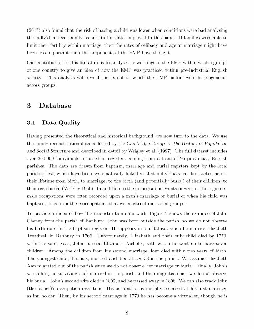
Figure 4 shows the predicted childlessness rate at ten years after marriage across social groups

(with average levels for parish and time period dummies) and highlights again the strong social

gradient in childlessness similar to celibacy. Marriages in wealthier social groups were more

1Note that childbirth outside of wedlock was banned by the Church of England, and that illegitimate births,therefore, were rare ranging from 1.2 per cent to 6.0 per cent of births across our period (Wrigley et al., 1997,pp. 224).

2A classic study of natural sterility is by Leridon (2008). He uses the Henry database, which consists of datafor rural France from the 18th century, when fertility control was ineffective. Restricting the sample to coupleswhere the husband and the wife were still living together at age 50, 3.7 per cent of women who married at age20-24 remained childless.

17

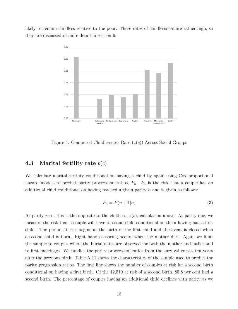
likely to remain childless relative to the poor. These rates of childlessness are rather high, so

they are discussed in more detail in section 6.

0.05

0.07

0.09

0.11

0.13

0.15

0.17

Unknown Labourers,Servants

Husbandmen Craftsmen Traders Farmers Merchants,Professionals

Gentry

Figure 4: Computed Childlessness Rate (z(c)) Across Social Groups

4.3 Marital fertility rate b(c)

We calculate marital fertility conditional on having a child by again using Cox proportional

hazard models to predict parity progression ratios, Pn. Pn is the risk that a couple has an

additional child conditional on having reached a given parity n and is given as follows:

Pn = P (n + 1|n) (3)

At parity zero, this is the opposite to the childless, z(c), calculation above. At parity one, we

measure the risk that a couple will have a second child conditional on them having had a first

child. The period at risk begins at the birth of the first child and the event is closed when

a second child is born. Right hand censoring occurs when the mother dies. Again we limit

the sample to couples where the burial dates are observed for both the mother and father and

to first marriages. We predict the parity progression ratios from the survival curves ten years

after the previous birth. Table A.11 shows the characteristics of the sample used to predict the

parity progression ratios. The first line shows the number of couples at risk for a second birth

conditional on having a first birth. Of the 12,519 at risk of a second birth, 85.8 per cent had a

second birth. The percentage of couples having an additional child declines with parity as we

18

would expect.

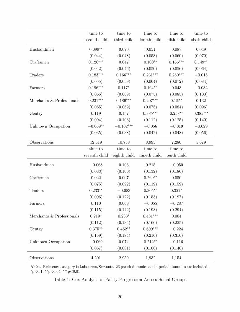
Table 4 shows the coefficients of Cox regressions modelling the probability to move to the next

parity conditionally on having one to nine children. We stop the estimation at P (10|9) because

after parity ten the sample size becomes too small. Here we see that the Gentry, and to a lesser

extent, the Merchants and Professionals, have higher probabilities to have an additional child,

in particular when they already have three.

The proportionality of the hazard rates is less clearly supported for the birth estimations than

for the two extensive margins. Among the 63 coefficients in Table 4, proportionality is rejected

in 26 cases (at the 5% level). However, this non-proportionality is not overly concerning because

we are estimating the parity progression ratios over a short period of time (the cumulated hazard

over ten years rather than 30 years for marriage rates), and non-proportionality is less likely to

be an issue on short time intervals (Bellera et al. 2010).

Table 5 shows the predicted parity progression ratios for various social groups from the re-

gressions of Table 4 assuming average levels for parish and time period dummies. Lower parity

progression ratios across the parities will produce a lower gross fertility rate for the social group.

Thus, at first glance there appears to be a social gradient with richer groups having higher fer-

tility. Following Henry(1953, chapter 14) and Feeney (1986), these parity progression ratios

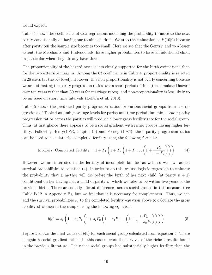
can be used to calculate the completed fertility using the following formula:

Mothers’ Completed Fertility = 1 + P1

(1 + P2

(1 + P3 . . .

(1 +

Pn

1− Pn

)))(4)

However, we are interested in the fertility of incomplete families as well, so we have added

survival probabilities to equation (4). In order to do this, we use logistic regression to estimate

the probability that a mother will die before the birth of her next child (at parity n + 1)

conditional on her having had a child of parity n, which we take to be within five years of the

previous birth. There are not significant differences across social groups in this measure (see

Table B.12 in Appendix B), but we feel that it is necessary for completeness. Thus, we can

add the survival probabilities sn to the completed fertility equation above to calculate the gross

fertility of women in the sample using the following equation:

b(c) = s0

(1 + s1P1

(1 + s2P2

(1 + s3P3 . . .

(1 +

snPn

1− snPn

))))(5)

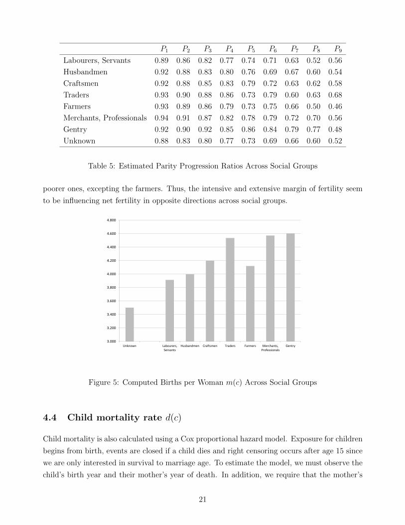
Figure 5 shows the final values of b(c) for each social group calculated from equation 5. There

is again a social gradient, which in this case mirrors the survival of the richest results found

in the previous literature. The richer social groups had substantially higher fertility than the

19

time to time to time to time to time to

second child third child fourth child fifth child sixth child

Husbandmen 0.099∗∗ 0.070 0.051 0.087 0.049

(0.044) (0.048) (0.053) (0.060) (0.070)

Craftsmen 0.126∗∗∗ 0.047 0.100∗∗ 0.166∗∗∗ 0.149∗∗

(0.042) (0.046) (0.050) (0.056) (0.064)

Traders 0.183∗∗∗ 0.166∗∗∗ 0.231∗∗∗ 0.280∗∗∗ −0.015

(0.055) (0.059) (0.064) (0.072) (0.084)

Farmers 0.196∗∗∗ 0.117∗ 0.164∗∗ 0.043 −0.032

(0.065) (0.069) (0.075) (0.085) (0.100)

Merchants & Professionals 0.231∗∗∗ 0.189∗∗∗ 0.207∗∗∗ 0.155∗ 0.132

(0.065) (0.069) (0.075) (0.084) (0.096)

Gentry 0.119 0.157 0.385∗∗∗ 0.258∗∗ 0.385∗∗∗

(0.094) (0.103) (0.112) (0.125) (0.140)

Unknown Occupation −0.069∗∗ −0.102∗∗∗ −0.056 −0.019 −0.029

(0.035) (0.038) (0.042) (0.048) (0.056)

Observations 12,519 10,738 8,993 7,280 5,679

time to time to time to time to

seventh child eighth child nineth child tenth child

Husbandmen −0.068 0.103 0.215 −0.050

(0.083) (0.100) (0.132) (0.186)

Craftsmen 0.022 0.007 0.269∗∗ 0.050

(0.075) (0.092) (0.119) (0.159)

Traders 0.233∗∗ −0.083 0.305∗∗ 0.327∗

(0.096) (0.122) (0.153) (0.197)

Farmers 0.110 0.069 −0.055 −0.287

(0.115) (0.142) (0.198) (0.294)

Merchants & Professionals 0.219∗ 0.233∗ 0.481∗∗∗ 0.004

(0.112) (0.134) (0.166) (0.225)

Gentry 0.375∗∗ 0.462∗∗ 0.699∗∗∗ −0.224

(0.159) (0.184) (0.216) (0.316)

Unknown Occupation −0.069 0.074 0.212∗∗ −0.116

(0.067) (0.081) (0.106) (0.146)

Observations 4,201 2,959 1,932 1,154

Notes: Reference category is Labourers/Servants. 26 parish dummies and 4 period dummies are included.∗p<0.1; ∗∗p<0.05; ∗∗∗p<0.01

Table 4: Cox Analysis of Parity Progression Across Social Groups

20

P1 P2 P3 P4 P5 P6 P7 P8 P9

Labourers, Servants 0.89 0.86 0.82 0.77 0.74 0.71 0.63 0.52 0.56

Husbandmen 0.92 0.88 0.83 0.80 0.76 0.69 0.67 0.60 0.54

Craftsmen 0.92 0.88 0.85 0.83 0.79 0.72 0.63 0.62 0.58

Traders 0.93 0.90 0.88 0.86 0.73 0.79 0.60 0.63 0.68

Farmers 0.93 0.89 0.86 0.79 0.73 0.75 0.66 0.50 0.46

Merchants, Professionals 0.94 0.91 0.87 0.82 0.78 0.79 0.72 0.70 0.56

Gentry 0.92 0.90 0.92 0.85 0.86 0.84 0.79 0.77 0.48

Unknown 0.88 0.83 0.80 0.77 0.73 0.69 0.66 0.60 0.52

Table 5: Estimated Parity Progression Ratios Across Social Groups

poorer ones, excepting the farmers. Thus, the intensive and extensive margin of fertility seem

to be influencing net fertility in opposite directions across social groups.

3.000

3.200

3.400

3.600

3.800

4.000

4.200

4.400

4.600

4.800

Unknown Labourers,Servants

Husbandmen Craftsmen Traders Farmers Merchants,Professionals

Gentry

Figure 5: Computed Births per Woman m(c) Across Social Groups

4.4 Child mortality rate d(c)

Child mortality is also calculated using a Cox proportional hazard model. Exposure for children

begins from birth, events are closed if a child dies and right censoring occurs after age 15 since

we are only interested in survival to marriage age. To estimate the model, we must observe the

child’s birth year and their mother’s year of death. In addition, we require that the mother’s

21

year of death is 15 years after the child’s birth. This requirement ensures that all of the child’s

mortality exposure was in the observed parish since the father may have moved the family after

the mother’s death. Children who we do not observe dying are assumed to have survived to

age 15. We take the predicted mortality rate from the survival curve at age 15. Table A.10

shows the characteristics of the sample used to estimate child deaths. Of the 48,865 children

at risk in the sample, we have a death rate of 26.0 per cent.

Specification (3) in Table 3 shows that there is no significant social gradient in child mortality.

All of the coefficients are insignificant and very close to zero. Moreover, the proportionality

of hazards is never rejected. Thus, differences in net fertility across groups do not seem to be

related to differences in relative survival of the rich and poor.

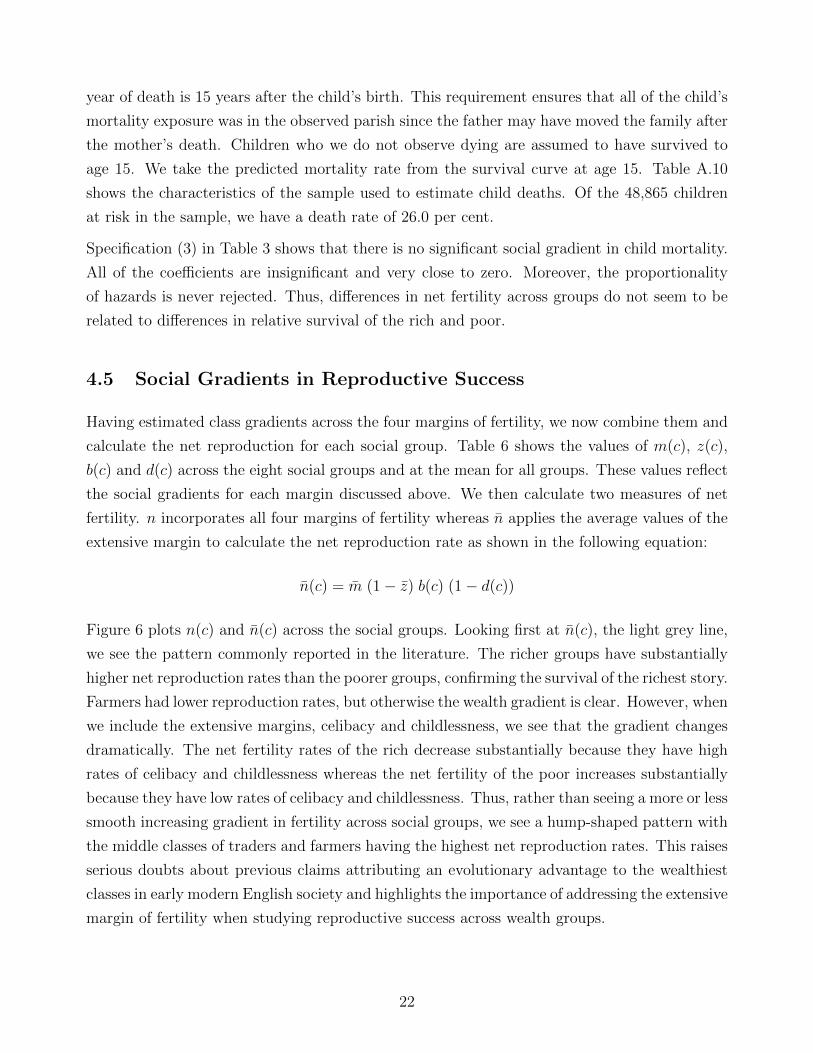
4.5 Social Gradients in Reproductive Success

Having estimated class gradients across the four margins of fertility, we now combine them and

calculate the net reproduction for each social group. Table 6 shows the values of m(c), z(c),

b(c) and d(c) across the eight social groups and at the mean for all groups. These values reflect

the social gradients for each margin discussed above. We then calculate two measures of net

fertility. n incorporates all four margins of fertility whereas n applies the average values of the

extensive margin to calculate the net reproduction rate as shown in the following equation:

n(c) = m (1− z) b(c) (1− d(c))

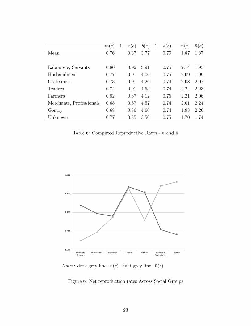
Figure 6 plots n(c) and n(c) across the social groups. Looking first at n(c), the light grey line,

we see the pattern commonly reported in the literature. The richer groups have substantially

higher net reproduction rates than the poorer groups, confirming the survival of the richest story.

Farmers had lower reproduction rates, but otherwise the wealth gradient is clear. However, when

we include the extensive margins, celibacy and childlessness, we see that the gradient changes

dramatically. The net fertility rates of the rich decrease substantially because they have high

rates of celibacy and childlessness whereas the net fertility of the poor increases substantially

because they have low rates of celibacy and childlessness. Thus, rather than seeing a more or less

smooth increasing gradient in fertility across social groups, we see a hump-shaped pattern with

the middle classes of traders and farmers having the highest net reproduction rates. This raises

serious doubts about previous claims attributing an evolutionary advantage to the wealthiest

classes in early modern English society and highlights the importance of addressing the extensive

margin of fertility when studying reproductive success across wealth groups.

22

m(c) 1− z(c) b(c) 1− d(c) n(c) n(c)

Mean 0.76 0.87 3.77 0.75 1.87 1.87

Labourers, Servants 0.80 0.92 3.91 0.75 2.14 1.95

Husbandmen 0.77 0.91 4.00 0.75 2.09 1.99

Craftsmen 0.73 0.91 4.20 0.74 2.08 2.07

Traders 0.74 0.91 4.53 0.74 2.24 2.23

Farmers 0.82 0.87 4.12 0.75 2.21 2.06

Merchants, Professionals 0.68 0.87 4.57 0.74 2.01 2.24

Gentry 0.68 0.86 4.60 0.74 1.98 2.26

Unknown 0.77 0.85 3.50 0.75 1.70 1.74

Table 6: Computed Reproductive Rates - n and n

1.900

2.000

2.100

2.200

2.300

Labourers,Servants

Husbandmen Craftsmen Traders Farmers Merchants,Professionals

Gentry

Notes: dark grey line: n(c). light grey line: n(c)

Figure 6: Net reproduction rates Across Social Groups

23

5 Migration and Selection

Any analysis of family reconstitution data faces the problem that people who migrate to or

from observed parishes are censored with regards to certain information. In the English data

there is no foolproof way of measuring migration since the English parish register system did

not include migration lists like the ones kept in Sweden (Jeub 1993). This makes it difficult to

calculate precise periods of exposure for each individual in the parish and is a limitation that

applies equally to the fertility and mortality calculations in Wrigley et al. (1997).3 However,

we do observe migration of a type because we know whether someone was baptised, married or

buried in the parish. Thus, we might not observe the baptism date of in-migrants, but we are

likely to observe their marriage, the baptism of their children or their burial. For out-migrants,

we would observe their baptism and/or marriage but not their burial. These three vital events

provide important information that can be incorporated in defining exposure periods. For

instance, there is no problem in measuring marital fertility if we observe a woman’s marriage

date, the baptism dates of her children and her burial date since she is very likely to have spent

her reproductive years in the parish. Childlessness and child mortality are similarly easy to

measure. However, it is important to note that we can only calculate these figures for non-

migrants and in-migrants and must exclude out-migrants since we cannot be sure they baptised

all of their children in the parish.

We run into more trouble when trying to measure celibacy rates in the data. As mentioned

above, we observe never-married (celibate) individuals based on three criteria: they were bap-

tised and buried in the parish; they survived past the age of 15; and they never married nor

baptised or buried any children in the parish. These three components ensure that we have

identified someone who never married and did not have any illegitimate children. Because we

need to observe both the baptism and burial date of an individual, to measure celibacy we have

to exclude both out-migrants and in-migrants from the calculations. Thus, because we must

exclude some form of migrants from all of the calculations, it is important to try to establish

that the selection bias of migrants is not driving our primary results, i.e. class-gradients in the

four margins.

Before conducting some empirical tests, it might be helpful to describe who the out- and in-

migrants were. Migrants in early modern England could have been one of three types. The

first type were people who did not move very far, for instance to a nearby parish, but fell

out of observation because their vital events were no longer being recorded in an observed

parish. These migrants were likely taking advantage of new economic opportunities such as

3Ruggles (1992) and Wrigley (1994) have also discussed potential migration biases to mean ages at marriageand death in reconstitution studies. These are discussed in more detail in Appendix C.

24

employment as a servant in a different parish but did not substantially vary their cultural

practices (Anderson, 1990, p. 11). These migrants were not insubstantial. Clark (1979) studied

the migration patterns of rural witnesses in diocesan courts between 1660 and 1730 finding that

70 per cent had moved at least once in their life. However, only 14 per cent had moved beyond

their county of origin. Likewise, Anderson (1990) found that two-thirds of rural migrants in

1851 moved less than 25 km. This evidence from 1851 is especially striking since migration had

increased substantially by this period driven by the growth of industrial cities (Shaw-Taylor

and Wrigley 2014). In our data, we can capture the demographic behaviour of this type of

migrant by looking at in-migrants to our own parishes, who are likely similar to out-migrants

from our parishes who also moved to similar parishes.

The second type of migrants were people who left home to become apprentices and learn a

trade. Minns and Wallis (2012) estimate that in 1700 around 9 per cent of English young

men were apprenticed in London alone and 60 per cent of these apprentices were in-migrants

to London. There were also opportunities for apprenticeship outside of London in provincial

towns and other larger cities such as Bristol, but these were small relative to the market in

London (Minns and Wallis 2012). The London apprenticeship market was remarkably open with

the majority of apprentices being unrelated to their master by kinship or place of origin and

drawn from nearly all of England, though with a clear gradient based on distance to London.

Apprentices came from all social backgrounds but the sons of gentlemen, professionals, traders

and craftsmen were over-represented among London apprentices relative to labourers, servants,

husbandmen and farmers (Leunig, Minns, and Wallis 2011). Thus, apprentices may account for

more migration among the higher and middle classes compared to the lower classes, excluding

farmers. There were also different social practices in choosing which sons were apprenticed.

Gentry rarely apprenticed their first son because in a system of primogeniture he was needed to

inherit the family’s estate and conduct its business. However, the further down the birth order

one traveled, the more gentry sons were apprenticed (Wallis and Webb 2011). Apprenticeship

among the middle classes was more likely to be based on merit and ability because there was

not a strong bias against apprenticing first-born sons. The poor on the other hand may have

favoured first born sons (Klemp et al. 2013). One should also note that a large minority of

these apprentices returned to their original parish after their apprenticeship, so not all of these

migrants were lost from observation forever (Klemp et al. 2013).

The third type of migrants were people who moved from our provincial parishes to towns or

larger population centres, London being the largest draw, but did not take part in formal ap-

prenticeships. Unfortunately, it is difficult to measure migration systematically in the early

modern period, but as mentioned above there is substantial evidence that migration was com-

mon (Schofield, 1970; Clark and Souden, 1988). We do not have precise information on rural

25

to urban migration until the mid-nineteenth century with the census of 1851. This data is an

imperfect proxy for our earlier period because of the enormous population growth and urban-

isation that occurred in England along with the Industrial Revolution, so we must interpret

the findings cautiously. According to a national sample analysed by Anderson (1990), 54 per

cent of the population lived more than 2 km from their place of birth. While two-thirds of

rural migrants moved less than 25 km, the percentages urban migrants moving less than 25

km were much lower: around 40 per cent of urban migrants to provincial cities and 20 per

cent of migrants to London (Anderson, 1990, pp. 11-12). Thus, as expected urban migrants

travelled longer distances than rural migrants, though this is for a much later period. Another

long-standing feature of urban migration was the extremely high death rates of migrants in

their new urban environment. Death rates in London were astoundingly high in the seven-

teenth century even as the population of London doubled across the century (Landers, 1993,

pp. 193-195; Shaw-Taylor and Wrigley, 2014, p. 76). High mortality meant that many of the

urban migrants would not have survived to reproduce anyway.

Keeping these three types of migrants in mind, we can now discuss how selective migration

might influence our results. We will begin by discussing our celibacy calculation from which we

have to exclude both in- and out-migrants. It is highly possible that some women permanently

left their parish of origin and never married or had children. However, this would only distort

our estimation of the celibacy margin across social groups if there were (i) different migration

rates for women across the social groups or if (ii) the women migrating from a particular social

group were more likely to remain celibate than women migrating from another group. On the

first point, we test whether there were significant differences in out-migration rates by class.

To do this, we have to categorise individuals by their father’s occupation since we are unable

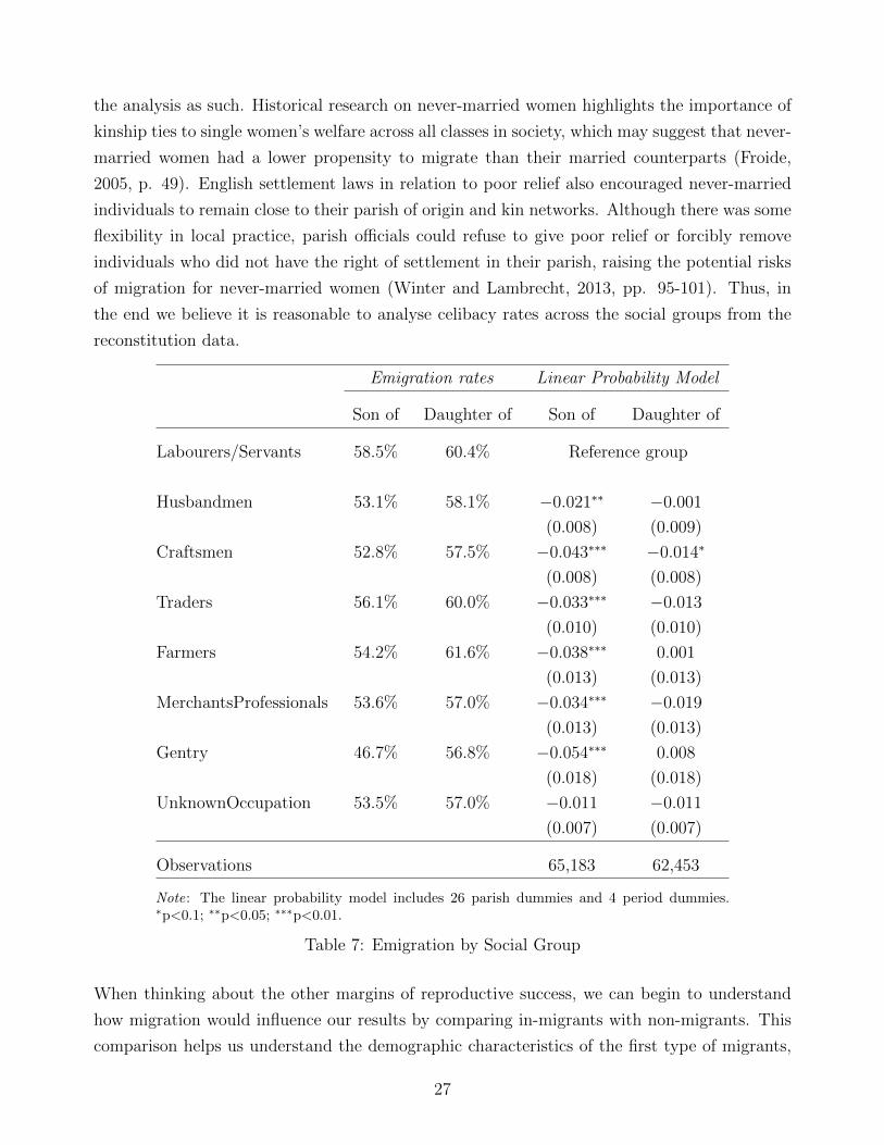
to observe the occupation of out-migrants at marriage. Table 7 illustrates two main features

of early modern migration: women were slightly more likely to emigrate than men and the

social gradient was largely flat for women and slightly decreasing for men. These gradients

are confirmed by linear probability models reported in the last two columns of Table 7. The

results suggest that the propensity to emigrate was statistically higher for male offspring born to

labourers and servants than for offspring of more well-off families, but there were no statistically

significant differences in emigration rates of female offspring (with the exception of the less

mobile daughters of craftsmen). This conclusion is reassuring for our analysis of fertility, which

mainly relied on information about women.

Unfortunately, it is much more difficult to deal with the second issue above. We have no way

of formally testing whether migrant women from different classes had the same or different

propensities to be celibate. We simply have to assume that celibate women’s propensity to

migrate was equal (or proportionally equal) to the propensities of non-migrants and conduct

26

the analysis as such. Historical research on never-married women highlights the importance of

kinship ties to single women’s welfare across all classes in society, which may suggest that never-

married women had a lower propensity to migrate than their married counterparts (Froide,

2005, p. 49). English settlement laws in relation to poor relief also encouraged never-married

individuals to remain close to their parish of origin and kin networks. Although there was some

flexibility in local practice, parish officials could refuse to give poor relief or forcibly remove

individuals who did not have the right of settlement in their parish, raising the potential risks

of migration for never-married women (Winter and Lambrecht, 2013, pp. 95-101). Thus, in

the end we believe it is reasonable to analyse celibacy rates across the social groups from the

reconstitution data.

Emigration rates Linear Probability Model

Son of Daughter of Son of Daughter of

Labourers/Servants 58.5% 60.4% Reference group

Husbandmen 53.1% 58.1% −0.021∗∗ −0.001

(0.008) (0.009)

Craftsmen 52.8% 57.5% −0.043∗∗∗ −0.014∗

(0.008) (0.008)

Traders 56.1% 60.0% −0.033∗∗∗ −0.013

(0.010) (0.010)

Farmers 54.2% 61.6% −0.038∗∗∗ 0.001

(0.013) (0.013)

MerchantsProfessionals 53.6% 57.0% −0.034∗∗∗ −0.019

(0.013) (0.013)

Gentry 46.7% 56.8% −0.054∗∗∗ 0.008

(0.018) (0.018)

UnknownOccupation 53.5% 57.0% −0.011 −0.011

(0.007) (0.007)

Observations 65,183 62,453

Note: The linear probability model includes 26 parish dummies and 4 period dummies.∗p<0.1; ∗∗p<0.05; ∗∗∗p<0.01.

Table 7: Emigration by Social Group

When thinking about the other margins of reproductive success, we can begin to understand

how migration would influence our results by comparing in-migrants with non-migrants. This

comparison helps us understand the demographic characteristics of the first type of migrants,

27

migrants who did not move very far, highlighted above. Appendix C provides the details of

these calculations, which follow a similar format to the general estimations conducted above.

We find that in-migrants had a higher propensity to be childless, but this did not vary across

the social groups. When looking at the number of children born to married women, we again

find that the gradient across social groups is more or less the same between in-migrants and

non-migrants even if in-migrants had slightly lower fertility. The wealth gradient of mortality

under the age of 15 was also the same, though migrants had a slightly higher propensity for

child deaths. Thus, it is likely that in-migrants had somewhat lower net reproduction than

non-migrants, but this did not vary across the wealth groups and therefore does not influence

our main results.

Clearly, migration could pose a potential threat to inference using reconstitution data, but

examining the historical record and conducting some substantial robustness checks leads us to

believe that migration would not strongly influence the social gradient in the four margins of

reproductive success. In the end, this reconstitution data is the only source available that can

be used to calculate the four margins of fertility in early modern England, so these relatively

minor assumptions seem reasonable.

6 Discussion of the results

As was reported earlier, we find that incorporating the extensive margins of fertility shifts our

understanding of the reproductive success of different socio-economic groups significantly. To

simplify the interpretations, we collapse our seven social groups into three classes: the lower

classes made up of labourers, husbandman, and craftsmen; the middle classes consisting of

traders and farmers; and the upper classes comprising the gentry and the merchants. Our

analyses above showed that these three social classes operated by means of distinctly different

demographic regimes. Although the families of all three classes married comparatively late

in life on average (Table B.13 in Appendix B), the upper classes were more often unmarried

or childless than the rest (Figures 3 and 4). This resulted in comparatively modest rates of

reproduction among the upper classes (Figure 6). Similarly, the lower classes had lower rates of

reproduction than their middle-class counterparts, but their lower net reproduction was caused

by fewer births within marriage rather than fertility control on the extensive margin (Figure 5).

Among middle-class families, however, birth limitation did not occur to the same extent as

in upper- and lower-class families. Farmers, although they had fewer births on average than

the upper classes, tended to marry comparatively more often. Traders had as many births

on average as the upper classes, but had lower rates of childlessness. These socio-specific

28

combinations gave the middle class the upper hand in the grand scheme of reproductive success

(Figure 6).

This general overview raises two sets of questions about our findings. First, what explains

class differentials in childlessness? For many of the social gradients above, it is fairly easy

to understand how they could emerge across the different groups. Marriage rates could be

influenced by cultural practices and requirements to save enough resources before marriage.

Sibship size could be influenced by differing mean ages at marriage and birth spacing across

the groups. However, it is slightly more difficult to explain variations in childlessness across

groups. In a time before effective contraception, it was difficult for couples who were sexually

active to avoid pregnancy over a long marriage. Thus, we will look at potential mechanisms

behind our childlessness findings to help explain variations in this margin. Second, how do these

findings relate to earlier studies attributing pre-Industrial economic development in North-West

Europe to the European Marriage Pattern? Dennison and Ogilvie (2014) have argued that the

differences in demographic behaviour and household structure were not as strong across Europe

as Hajnal (1965) and later authors have suggested. However, our study allows us to look at

differences in these structures within a society and speculate on how they may have influenced

economic growth.

6.1 Possible Reasons for High Childlessness

One of the more puzzling findings presented above was the strong variations in childlessness by

social group. Thus, in this section we will consider a number of potential explanations for the

social gradient in childlessness in turn, though our analysis does not allow us to fully identify

the causal pathway running from higher social status to higher childlessness.

Before considering potential mechanisms, we must first show that that our rates of childlessness

are not a product of potential measurement error in our data. The childlessness rates could be

skewed if the sources of occupations, from marriages, baptisms, or deaths, were significantly

different across social groups. In fact, a large proportion of our occupational data comes from

baptism records, which would only be recorded for individuals who were not childless. This may

explain the significantly higher rate of childlessness among those with an unknown occupation.

In order to test whether this was the case, we restricted our analysis to father’s occupations

that were drawn from marriage or burial registers and moved those from baptism registers into

the unknown occupation category. The results for childlessness are reported in Appendix D,

Table D.19. Removing the baptism occupations, reduces the slope of the gradient of childless-

ness across social groups and some of the differences between groups become insignificant, but

the result for the gentry remains. Importantly, the coefficient for the unknown occupations is

29

no longer significant and is substantially below that of the gentry. Thus, we believe that our

result of higher childlessness for the upper classes is a real difference in the childlessness rate.

The high level of childlessness that we measure is also similar (if slightly lower) to the child-

lessness observed for the British peerage in the pre-Industrial period where childlessness rates

could reach 24 per cent (Hollingsworth, 1965, p. 46). We perform a similar robustness check

for marital fertility rates and find that the slightly lower fertility of the unknown occupation

group was also partly a product of the greater propensity to observe a father’s occupation if he

had more children (see Figure D.8).

Having shown that the social gradient in childlessness is not an artefact of the way occupations

were recorded in the data, we now turn to other alternative mechanisms. First, Wrigley et al.

(1997, pp. 394-8) argue that the most important variable influencing entry sterility (or the

inability to produce any child in a marriage) was the mother’s age at marriage. Thus, if women

in higher social groups married systematically later than their lower social group peers, then

we would expect to see a higher rate of childlessness. However, this cannot explain the higher

childlessness rates among merchants and professionals and the gentry since they had similar

mean ages of marriage to some of the other social groups (Table B.13).

Second, Gobbi and Goni (2016) suggest that inheritance practices may have influenced whether

couples remained childless. Before the twentieth century, the English nobility used marriage

settlements to pass land and wealth to their heir. Marriage settlements set up a trust where the

bride and groom were only life tenants to their estate and the estate was passed on unbroken

to the heir of their marriage. Marriage settlements were instigated at the marriage of an heir

(alternatively, settlements could be signed when the heir turn 21) and provided for the heir’s

younger brothers and sisters, effectively preventing the estate from being broken apart. They

had to be renewed every generation. Studying the British peerage between 1603 and 1938,

Gobbi and Goni found that the rates of childlessness among heirs without marriage settlements

were 8 to 13 per cent higher than rates among heirs with marriage settlements. Because the

estates of heirs without marriage settlements could be sold on the market, these heirs chose to

remain childless rather than pass on a smaller estate to their son and heir. An heir would not

have a marriage settlement if his father died before his marriage, which occurred in 23.6 per

cent of cases in Gobbi and Goni’s dataset. Thus, this inheritance structure, which would have

influenced the gentry most strongly, could have contributed to higher childlessness rates among

higher wealth groups in our data.

It is also possible that higher rates of venereal diseases such as gonorrhoea, chlamydia and

syphilis among the upper classes led to higher rates of sterility. Gonorrhoea and chlamydia lead

to infertility by preventing conception since both diseases if untreated lead to blockages of the

Fallopian tubes and abnormal sperm, whereas syphilis causes higher rates of miscarriages and

30

stillbirths (Belsey, 1976, pp. 327-29). There is anecdotal evidence that some of these diseases

were prevalent among the gentry and aristocracy, e.g. Henry VIII had syphilis (Parascandola

2008) and James Boswell, a high-born Scottish lawyer, had at least 17 infections of gonorrhoea

in his life (Stone, 1979, p. 350). However, it is much more difficult to find prevalence estimates

for the general population. Szreter (2017) found that in the 1770s 8 per cent of residents in

Cheshire had contracted syphilis by the age of 35, but the prevalence rate was much lower at

1 per cent in Cheshire’s rural hinterlands similar to most of the parishes in the reconstitution

dataset. There is no systematic information about class gradients in syphilis prevalence until

the early twentieth century when syphilis was most common among unskilled working-class men

(Szreter, 2014) and therefore would not explain higher rates of childlessness among the upper

classes. Prevalence rates of gonorrhoea and chlamydia were likely higher than for syphilis, but

again we have no way of knowing whether these also produced a class gradient.

Goni (2015) has also argued that consanguinity could have influenced childlessness. Again,

studying the British peerage, now in the nineteenth century, he found that children of con-

sanguineous marriages (between second cousins or closer) were 50 per cent more likely to be

childless than children of peers who did not marry in the same family. Thus, if members of the

gentry were more likely to marry individuals closely related to them, this could explain part of

the difference in childlessness that we observe.

Finally, it is possible that the unique cultural context of marriage among the gentry led to higher

levels of childlessness. Since members of the wealthier classes had less control over who they

married, they may have ended up in loveless marriages at a higher rate than their counterparts

down the social ladder (Stone, 1979, p. 308). Thus, if their rates of sexual activity were lower

and they stopped having sexual intercourse at an earlier point in the marriage, then this might

increase rates of childlessness enough to reflect the differences we have observed. Another

potential explanation has to do with the amount of time that husbands and wives were living

apart. If the husband were constantly traveling to oversee estates or conduct business across his

wide holdings, this could also reduce the frequency of sexual intercourse. However, this would

also affect agricultural labourers who may have travelled at harvest time in search of work.

In addition, it is possible that the more educated women of the higher wealth groups could have

been partially responsible for childlessness. Bree and de la Croix (2016) argue that the rise of

childlessness observed in Rouen might have been driven by wives who did not want to deform

their bodies or have the burden of a pregnant belly. The risk of maternal mortality could also

have led some women from the upper class to fear childbearing.

In the end, the increased childlessness among the gentry is likely caused by a number of these

factors combined. Thus, the 5 percentage point difference in childlessness rates between the

31

wealthy and poor could have been driven by slight differences in marriage age, inheritance

patterns, venereal infections, consanguinity and sexual activity that accumulated to the final

effect.

6.2 The European Marriage Pattern and Economic Growth

In addition our study makes two important contributions to the debate on the foundations of

North-West European economic success. First, it suggests that the different features of the

European Marriage Pattern were used differently by different social groups even within the

boundaries of a single economy such as England’s. Thus, the previous literature’s analysis at

national borders may not be helpful in examining how family formation and structure influ-

enced economic development. Second, we argue that the class-specific demographic patterns

in England were particularly conducive to its industrial development shortly after our period.

Rather than survival of the richest, the higher reproductive success of the middle classes ensured

that those most likely to invest in the human capital of their children outgrew other groups.

Previous studies have considered these questions in the context of a Malthusian model (e.g.

Voigtlander and Voth 2013; Sharp, Strulik, and Weisdorf 2012). Technological innovations or

extensive expansion of land under production could lead to temporary increases in income,

but rising birth rates (and survival rates of children) eventually led the population to increase

driving wages back down to subsistence. Thus, if the population is able to limit its births at any

wage rate in this Malthusian equilibrium, then the equilibrium wage rate will rise, consistent

with economic growth. Traditionally, scholars held that births could only be limited by raising

the age of marriage or increasing the celibacy rate (Wrigley and Schofield, 1981; Weir, 1984).

We depart from the view inherent in these previous approaches that families were more or

less homogenous or at least demographically similar. The substantially different demographic

behaviour of the various wealth groups produced different equilibria for various social groups

in the economy. Each would respond differently to changes in economic conditions which

might accentuate or diminish the influence of one particular mechanism in limiting fertility. By

our estimation, celibacy and childlessness were concentrated at the upper echelons of society

with fewer people in the lower classes using these as a fertility limitation strategy. Toward

the bottom of the social ladder birth limitation took place through a reduction in marital

fertility. These findings correspond well to several recent papers which showed that birth

spacing only responded to real wages and prices among lower class families in pre-Industrial

England and Sweden (Cinnirella, Klemp, and Weisdorf 2017; Bengtsson and Dribe 2006). Thus,

we do not argue that the aggregate accounting exercises, on celibacy for instance (Weir 1984;

Schofield 1985), are incorrect. Instead, there needs to be more care taken in how these different

32

fertility limitation mechanisms influence the general economic development in the pre-Industrial

era. Thus, future studies on the European Marriage Pattern should focus more carefully on

establishing a more dynamic model for the marriage pattern that allows for variation within

countries and change in the intensity and consequences of the pattern over time.

Our results also highlight how the class-specific demographic patterns - with middle-class fam-

ilies being more successful in terms of reproduction than their upper and lower counterparts

- would be helpful for England’s economic growth. If middle-class families were the most re-

productively successful and also more prone to invest in growth-promoting education of their

offspring, then their reproductive success could create a growing pool of human capital in a

society. Lower-class families were rarely able to afford primary education let alone advanced

education such as apprenticeships (Minns and Wallis, 2012). On the other hand, while upper-

class families were able to afford to pay for growth-enhancing education and sent some of their

younger sons into apprenticeships, elder sons were mainly trained to take over their family’s

estates and did not need growth-promoting educational training: they relied on the rental in-

come of their estates and had no incentive to participate in activities that fostered economic

growth (Doepke and Zilibotti 2008; Wallis and Webb 2011). Crouzet’s famous study of the

social background of the emerging class of English industrialists confirms this view, showing

that less than three per cent of the new industrialists had an upper-class origin (Crouzet 1985).

Rather, 85 per cent of industrialists came from a middle-class background. More than 40 per

cent were involved in an industrial trade that was similar to that of their father and 22 per

cent had a father who was a farmer. It was the children of the middle-classes that helped drive

England’s industrial development, not those of the upper or lower classes.

This pattern of human capital investment emphasises how Hajnal’s European Marriage Pattern

might have been conducive to economic growth in the case of England: not because all English

families universally strove to limit births, but because those classes that invested comparatively

little in growth-promoting education were more inclined to engage in birth restricting practises.

In the English case, the survival of the richest was therefore not a growth-promoting strategy:

the survival of the middle-classes was. This support the hypothesis set forth by Galor and

Moav (2002) that quality-orientated families represent the leading trait in a society of economic

growth.

7 Conclusion

This paper has shown that when accounting for both the extensive and intensive margins of fer-

tility, the previous findings that the rich in early modern England had the highest reproductive

33

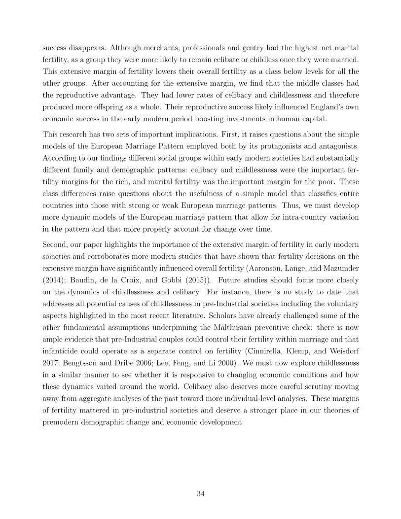
success disappears. Although merchants, professionals and gentry had the highest net marital

fertility, as a group they were more likely to remain celibate or childless once they were married.

This extensive margin of fertility lowers their overall fertility as a class below levels for all the

other groups. After accounting for the extensive margin, we find that the middle classes had

the reproductive advantage. They had lower rates of celibacy and childlessness and therefore

produced more offspring as a whole. Their reproductive success likely influenced England’s own

economic success in the early modern period boosting investments in human capital.

This research has two sets of important implications. First, it raises questions about the simple

models of the European Marriage Pattern employed both by its protagonists and antagonists.

According to our findings different social groups within early modern societies had substantially

different family and demographic patterns: celibacy and childlessness were the important fer-

tility margins for the rich, and marital fertility was the important margin for the poor. These

class differences raise questions about the usefulness of a simple model that classifies entire

countries into those with strong or weak European marriage patterns. Thus, we must develop

more dynamic models of the European marriage pattern that allow for intra-country variation

in the pattern and that more properly account for change over time.

Second, our paper highlights the importance of the extensive margin of fertility in early modern

societies and corroborates more modern studies that have shown that fertility decisions on the

extensive margin have significantly influenced overall fertility (Aaronson, Lange, and Mazumder

(2014); Baudin, de la Croix, and Gobbi (2015)). Future studies should focus more closely

on the dynamics of childlessness and celibacy. For instance, there is no study to date that

addresses all potential causes of childlessness in pre-Industrial societies including the voluntary

aspects highlighted in the most recent literature. Scholars have already challenged some of the

other fundamental assumptions underpinning the Malthusian preventive check: there is now

ample evidence that pre-Industrial couples could control their fertility within marriage and that

infanticide could operate as a separate control on fertility (Cinnirella, Klemp, and Weisdorf

2017; Bengtsson and Dribe 2006; Lee, Feng, and Li 2000). We must now explore childlessness

in a similar manner to see whether it is responsive to changing economic conditions and how

these dynamics varied around the world. Celibacy also deserves more careful scrutiny moving

away from aggregate analyses of the past toward more individual-level analyses. These margins

of fertility mattered in pre-industrial societies and deserve a stronger place in our theories of

premodern demographic change and economic development.

34

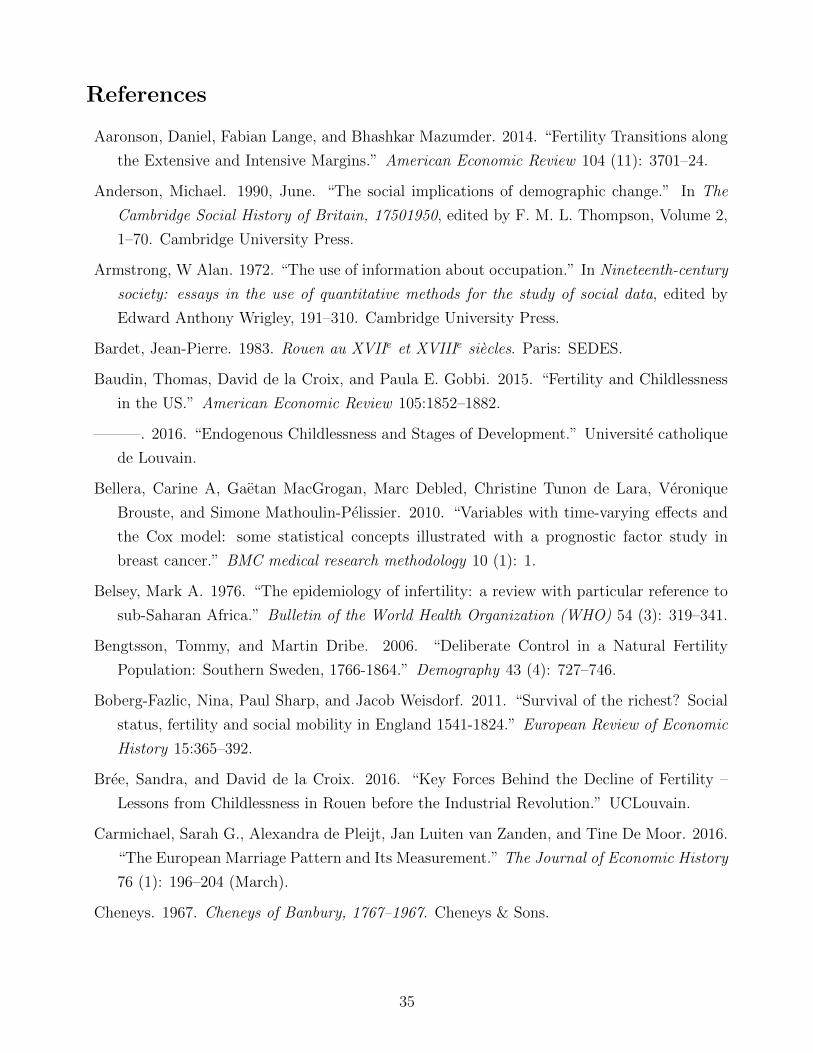
References

Aaronson, Daniel, Fabian Lange, and Bhashkar Mazumder. 2014. “Fertility Transitions along

the Extensive and Intensive Margins.” American Economic Review 104 (11): 3701–24.

Anderson, Michael. 1990, June. “The social implications of demographic change.” In The

Cambridge Social History of Britain, 17501950, edited by F. M. L. Thompson, Volume 2,

1–70. Cambridge University Press.

Armstrong, W Alan. 1972. “The use of information about occupation.” In Nineteenth-century

society: essays in the use of quantitative methods for the study of social data, edited by

Edward Anthony Wrigley, 191–310. Cambridge University Press.

Bardet, Jean-Pierre. 1983. Rouen au XVIIe et XVIIIe siecles. Paris: SEDES.

Baudin, Thomas, David de la Croix, and Paula E. Gobbi. 2015. “Fertility and Childlessness

in the US.” American Economic Review 105:1852–1882.

. 2016. “Endogenous Childlessness and Stages of Development.” Universite catholique

de Louvain.

Bellera, Carine A, Gaetan MacGrogan, Marc Debled, Christine Tunon de Lara, Veronique

Brouste, and Simone Mathoulin-Pelissier. 2010. “Variables with time-varying effects and

the Cox model: some statistical concepts illustrated with a prognostic factor study in

breast cancer.” BMC medical research methodology 10 (1): 1.

Belsey, Mark A. 1976. “The epidemiology of infertility: a review with particular reference to

sub-Saharan Africa.” Bulletin of the World Health Organization (WHO) 54 (3): 319–341.

Bengtsson, Tommy, and Martin Dribe. 2006. “Deliberate Control in a Natural Fertility

Population: Southern Sweden, 1766-1864.” Demography 43 (4): 727–746.

Boberg-Fazlic, Nina, Paul Sharp, and Jacob Weisdorf. 2011. “Survival of the richest? Social

status, fertility and social mobility in England 1541-1824.” European Review of Economic

History 15:365–392.

Bree, Sandra, and David de la Croix. 2016. “Key Forces Behind the Decline of Fertility –

Lessons from Childlessness in Rouen before the Industrial Revolution.” UCLouvain.

Carmichael, Sarah G., Alexandra de Pleijt, Jan Luiten van Zanden, and Tine De Moor. 2016.

“The European Marriage Pattern and Its Measurement.” The Journal of Economic History

76 (1): 196–204 (March).

Cheneys. 1967. Cheneys of Banbury, 1767–1967. Cheneys & Sons.

35

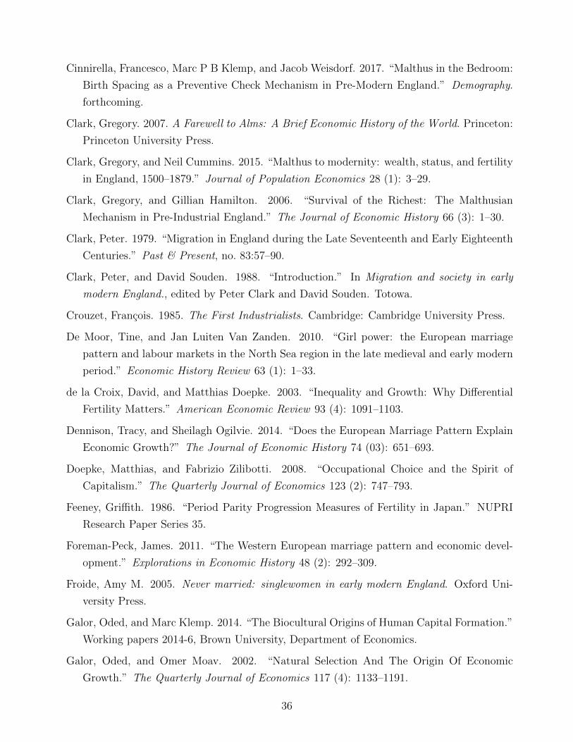
Cinnirella, Francesco, Marc P B Klemp, and Jacob Weisdorf. 2017. “Malthus in the Bedroom:

Birth Spacing as a Preventive Check Mechanism in Pre-Modern England.” Demography.

forthcoming.

Clark, Gregory. 2007. A Farewell to Alms: A Brief Economic History of the World. Princeton:

Princeton University Press.

Clark, Gregory, and Neil Cummins. 2015. “Malthus to modernity: wealth, status, and fertility

in England, 1500–1879.” Journal of Population Economics 28 (1): 3–29.

Clark, Gregory, and Gillian Hamilton. 2006. “Survival of the Richest: The Malthusian

Mechanism in Pre-Industrial England.” The Journal of Economic History 66 (3): 1–30.

Clark, Peter. 1979. “Migration in England during the Late Seventeenth and Early Eighteenth

Centuries.” Past & Present, no. 83:57–90.

Clark, Peter, and David Souden. 1988. “Introduction.” In Migration and society in early

modern England., edited by Peter Clark and David Souden. Totowa.

Crouzet, Francois. 1985. The First Industrialists. Cambridge: Cambridge University Press.

De Moor, Tine, and Jan Luiten Van Zanden. 2010. “Girl power: the European marriage

pattern and labour markets in the North Sea region in the late medieval and early modern

period.” Economic History Review 63 (1): 1–33.

de la Croix, David, and Matthias Doepke. 2003. “Inequality and Growth: Why Differential

Fertility Matters.” American Economic Review 93 (4): 1091–1103.

Dennison, Tracy, and Sheilagh Ogilvie. 2014. “Does the European Marriage Pattern Explain

Economic Growth?” The Journal of Economic History 74 (03): 651–693.

Doepke, Matthias, and Fabrizio Zilibotti. 2008. “Occupational Choice and the Spirit of

Capitalism.” The Quarterly Journal of Economics 123 (2): 747–793.

Feeney, Griffith. 1986. “Period Parity Progression Measures of Fertility in Japan.” NUPRI

Research Paper Series 35.

Foreman-Peck, James. 2011. “The Western European marriage pattern and economic devel-

opment.” Explorations in Economic History 48 (2): 292–309.

Froide, Amy M. 2005. Never married: singlewomen in early modern England. Oxford Uni-

versity Press.

Galor, Oded, and Marc Klemp. 2014. “The Biocultural Origins of Human Capital Formation.”

Working papers 2014-6, Brown University, Department of Economics.

Galor, Oded, and Omer Moav. 2002. “Natural Selection And The Origin Of Economic

Growth.” The Quarterly Journal of Economics 117 (4): 1133–1191.

36

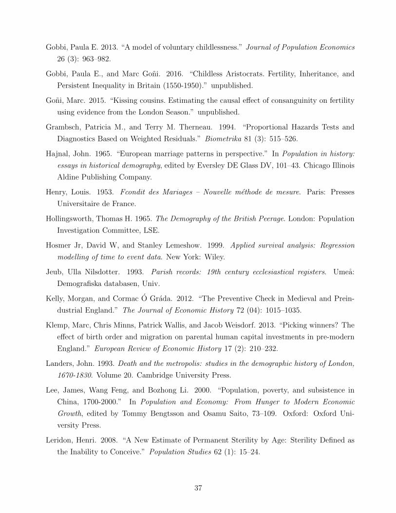
Gobbi, Paula E. 2013. “A model of voluntary childlessness.” Journal of Population Economics

26 (3): 963–982.

Gobbi, Paula E., and Marc Goni. 2016. “Childless Aristocrats. Fertility, Inheritance, and

Persistent Inequality in Britain (1550-1950).” unpublished.

Goni, Marc. 2015. “Kissing cousins. Estimating the causal effect of consanguinity on fertility

using evidence from the London Season.” unpublished.

Grambsch, Patricia M., and Terry M. Therneau. 1994. “Proportional Hazards Tests and

Diagnostics Based on Weighted Residuals.” Biometrika 81 (3): 515–526.

Hajnal, John. 1965. “European marriage patterns in perspective.” In Population in history:

essays in historical demography, edited by Eversley DE Glass DV, 101–43. Chicago Illinois

Aldine Publishing Company.

Henry, Louis. 1953. Fcondit des Mariages – Nouvelle methode de mesure. Paris: Presses

Universitaire de France.

Hollingsworth, Thomas H. 1965. The Demography of the British Peerage. London: Population

Investigation Committee, LSE.

Hosmer Jr, David W, and Stanley Lemeshow. 1999. Applied survival analysis: Regression

modelling of time to event data. New York: Wiley.

Jeub, Ulla Nilsdotter. 1993. Parish records: 19th century ecclesiastical registers. Umea:

Demografiska databasen, Univ.

Kelly, Morgan, and Cormac O Grada. 2012. “The Preventive Check in Medieval and Prein-

dustrial England.” The Journal of Economic History 72 (04): 1015–1035.

Klemp, Marc, Chris Minns, Patrick Wallis, and Jacob Weisdorf. 2013. “Picking winners? The

effect of birth order and migration on parental human capital investments in pre-modern

England.” European Review of Economic History 17 (2): 210–232.

Landers, John. 1993. Death and the metropolis: studies in the demographic history of London,

1670-1830. Volume 20. Cambridge University Press.

Lee, James, Wang Feng, and Bozhong Li. 2000. “Population, poverty, and subsistence in

China, 1700-2000.” In Population and Economy: From Hunger to Modern Economic

Growth, edited by Tommy Bengtsson and Osamu Saito, 73–109. Oxford: Oxford Uni-

versity Press.

Leridon, Henri. 2008. “A New Estimate of Permanent Sterility by Age: Sterility Defined as

the Inability to Conceive.” Population Studies 62 (1): 15–24.

37

Leunig, Tim, Chris Minns, and Patrick Wallis. 2011. “Networks in the Premodern Economy:

The Market for London Apprenticeships, 16001749.” The Journal of Economic History 71

(2): 413–443 (June).

Long, Jason. 2013. “The surprising social mobility of Victorian Britain.” European Review of

Economic History 17 (1): 1–23.

Malthus, Thomas. 1798. An Essay on the Principle of Population. London: Johnson.

Minns, Chris, and Patrick Wallis. 2012. “Rules and reality: quantifying the practice of

apprenticeship in early modern England.” The Economic History Review 65 (2): 556–579.

Mokyr, Joel. 2005. “Long-term economic growth and the history of technology.” In Handbook

of economic growth, edited by Philippe Aghion and Steven N. Durlauf, Volume 1, 1113–

1180. Elsevier.

Parascandola, John. 2008. Sex, sin, and science: a history of syphilis in America. Greenwood

Publishing Group.

Ruggles, Steven. 1992. “Migration, Marriage, and Mortality: Correcting Sources of Bias in

English Family Reconstitutions.” Population Studies 46 (3): 507–522.

Schoenfeld, David. 1982. “Partial Residuals for The Proportional Hazards Regression Model.”

Biometrika 69 (1): 239–241.

Schofield, Roger. 1971. “Age-specific mobility in an eighteenth century rural english parish.”

Annales de demographie historique 1970 (1): 261–274.

. 1985. “English marriage patterns revisited.” Journal of Family History 10:2–20.

Sharp, Paul, Holger Strulik, and Jacob Weisdorf. 2012. “The determinants of income in a

Malthusian equilibrium.” Journal of Development Economics 97 (1): 112–117.

Shaw-Taylor, Leigh, and Edward Anthony Wrigley. 2014. “Occupational structure and pop-

ulation change.” In The Cambridge Economic History of Modern Britain: Volume 1, In-

dustrialisation, 1700–1870, edited by Jane Humphries Roderick Floud and Paul Johnson,

53–88. Cambridge University Press.

Skirbekk, Vegard, et al. 2008. “Fertility trends by social status.” Demographic Research 18

(5): 145–180.

Squicciarini, Mara P., and Nico Voigtlander. 2015. “Human Capital and Industrialization:

Evidence from the Age of Enlightenment.” The Quarterly Journal of Economics 130 (4):

1825–1883.

Stone, Lawrence. 1979. The family sex and marriage: in England 1500-1800. New York:

Harper and Row.

38

Szreter, Simon. 2014. “The Prevalence of Syphilis in England and Wales on the Eve of

the Great War: Re-visiting the Estimates of the Royal Commission on Venereal Diseases

19131916.” Social History of Medicine 27 (3): 508–529.

. 2017. “Treatment Rates for the Pox in early modern England: a comparative estimate

of the prevalence of syphilis in the city of Chester and its rural vicinity in the 1770s.”

Continuity and Change. forthcoming.

Van Leeuwen, Marco HD, and Ineke Maas. 2011. HISCLASS: A historical international social

class scheme. Universitaire Pers Leuven.

Vogl, Tom. 2016. “Differential Fertility, Human Capital, and Development.” Review of

Economic Studies 83 (January): 365–401.

Voigtlander, Nico, and Hans-Joachim Voth. 2013. “The Three Horsemen of Riches: Plague,

War, and Urbanization in Early Modern Europe.” Review of Economic Studies 80 (2):

774–811.

Wallis, Patrick, and Cliff Webb. 2011. “The education and training of gentry sons in early

modern England.” Social History 36 (1): 36–53.

Weir, David R. 1984. “Rather never than late: celibacy and age at marriage in English cohort

fertility, 1541-1871.” Journal of Family History 9 (04): 340–54.

Winter, Anne, and Thijs Lambrecht. 2013. “Migration, Poor Relief and Local Autonomy: Set-

tlement Policies in England and the Southern Low Countries in the Eighteenth Century*.”

Past & Present 218 (1): 91–126.

Wrigley, Edward Anthony. 1966. “Family reconstitution.” In An Introduction to English

Historical Demography: From the Sixteenth to the Nineteenth Century, edited by David

Edward Charles Eversley, Peter Laslett, and Edward Anthony Wrigley, 96–159. London:

Weidenfeld and Nicolson.

. 1994. “The Effect of Migration on the Estimation of Marriage Age in Family Recon-

stitution Studies.” Population Studies 48 (1): 81–97.

Wrigley, Edward Anthony, R S Davies, James Oeppen, and Roger Schofield. 1997. English

Population History from Family Reconstitution: 1580–1837. Cambridge: Cambridge Uni-

versity Press.

Wrigley, Edward Anthony, and Roger Schofield. 1981. The population history of England

1541-1871: A Reconstruction. Cambridge University Press.

39

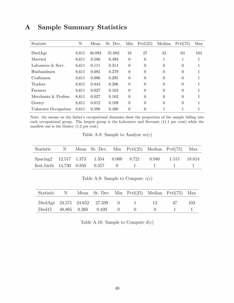
A Sample Summary Statistics

Statistic N Mean St. Dev. Min Pctl(25) Median Pctl(75) Max

DiedAge 8,611 46.093 21.082 16 27 43 64 104

Married 8,611 0.586 0.493 0 0 1 1 1

Labourers & Serv. 8,611 0.111 0.314 0 0 0 0 1

Husbandmen 8,611 0.085 0.279 0 0 0 0 1

Craftsmen 8,611 0.096 0.295 0 0 0 0 1

Traders 8,611 0.044 0.206 0 0 0 0 1

Farmers 8,611 0.027 0.163 0 0 0 0 1

Merchants & Profess. 8,611 0.027 0.162 0 0 0 0 1

Gentry 8,611 0.012 0.109 0 0 0 0 1

Unknown Occupation 8,611 0.598 0.490 0 0 1 1 1

Note: the means on the father’s occupational dummies show the proportion of the sample falling intoeach occupational group. The largest group is the Labourers and Servants (11.1 per cent) while thesmallest one is the Gentry (1.2 per cent).

Table A.8: Sample to Analyze m(c)

Statistic N Mean St. Dev. Min Pctl(25) Median Pctl(75) Max

Spacing2 12,517 1.373 1.354 0.000 0.721 0.940 1.515 18.014

first birth 14,730 0.850 0.357 0 1 1 1 1

Table A.9: Sample to Compute z(c)

Statistic N Mean St. Dev. Min Pctl(25) Median Pctl(75) Max

DiedAge 24,571 24.652 27.339 0 1 12 47 103

Died15 48,865 0.260 0.439 0 0 0 1 1

Table A.10: Sample to Compute d(c)

40

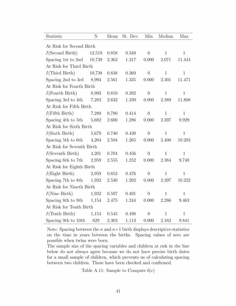
Statistic N Mean St. Dev. Min Median Max

At Risk for Second Birth

I(Second Birth) 12,519 0.858 0.349 0 1 1

Spacing 1st to 2nd 10,739 2.362 1.317 0.000 2.071 11.444

At Risk for Third Birth

I(Third Birth) 10,738 0.838 0.369 0 1 1

Spacing 2nd to 3rd 8,994 2.561 1.335 0.000 2.301 11.471

At Risk for Fourth Birth

I(Fourth Birth) 8,993 0.810 0.392 0 1 1

Spacing 3rd to 4th 7,283 2.632 1.339 0.000 2.389 11.808

At Risk for Fifth Birth

I(Fifth Birth) 7,280 0.780 0.414 0 1 1

Spacing 4th to 5th 5,682 2.600 1.286 0.000 2.397 9.929

At Risk for Sixth Birth

I(Sixth Birth) 5,679 0.740 0.439 0 1 1

Spacing 5th to 6th 4,204 2.594 1.265 0.000 2.400 10.203

At Risk for Seventh Birth

I(Seventh Birth) 4,201 0.704 0.456 0 1 1

Spacing 6th to 7th 2,959 2.555 1.252 0.000 2.384 9.748

At Risk for Eighth Birth

I(Eight Birth) 2,959 0.653 0.476 0 1 1

Spacing 7th to 8th 1,932 2.530 1.202 0.000 2.397 10.222

At Risk for Nineth Birth

I(Nine Birth) 1,932 0.597 0.491 0 1 1

Spacing 8th to 9th 1,154 2.475 1.244 0.000 2.286 9.463

At Risk for Tenth Birth

I(Tenth Birth) 1,154 0.545 0.498 0 1 1

Spacing 9th to 10th 629 2.303 1.113 0.000 2.162 9.841

Note: Spacing between the n and n+1 birth displays descriptive statisticson the time in years between the births. Spacing values of zero arepossible when twins were born.The sample size of the spacing variables and children at risk in the linebelow do not always agree because we do not have precise birth datesfor a small sample of children, which prevents us of calculating spacingbetween two children. These have been checked and confirmed.

Table A.11: Sample to Compute b(c)

41

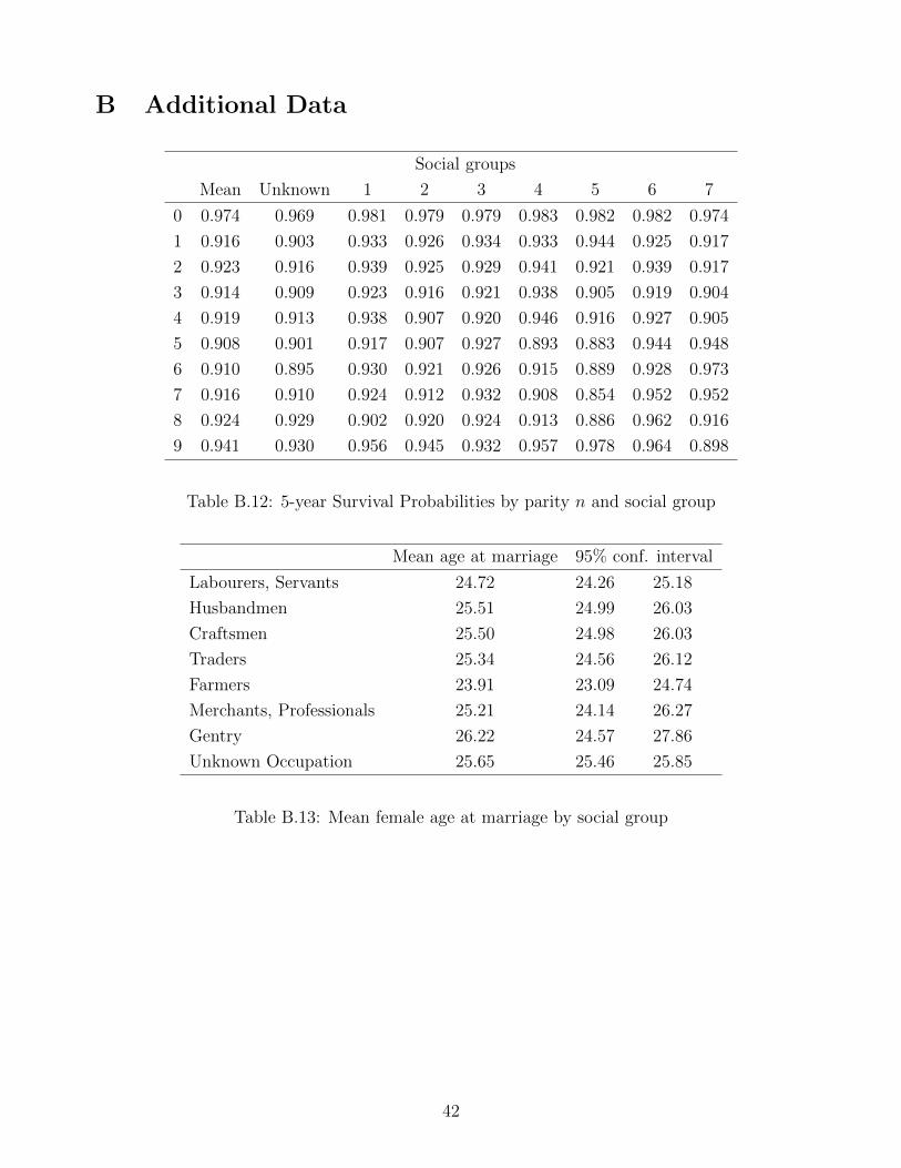
B Additional Data

Social groups

Mean Unknown 1 2 3 4 5 6 7

0 0.974 0.969 0.981 0.979 0.979 0.983 0.982 0.982 0.974

1 0.916 0.903 0.933 0.926 0.934 0.933 0.944 0.925 0.917

2 0.923 0.916 0.939 0.925 0.929 0.941 0.921 0.939 0.917

3 0.914 0.909 0.923 0.916 0.921 0.938 0.905 0.919 0.904

4 0.919 0.913 0.938 0.907 0.920 0.946 0.916 0.927 0.905

5 0.908 0.901 0.917 0.907 0.927 0.893 0.883 0.944 0.948

6 0.910 0.895 0.930 0.921 0.926 0.915 0.889 0.928 0.973

7 0.916 0.910 0.924 0.912 0.932 0.908 0.854 0.952 0.952

8 0.924 0.929 0.902 0.920 0.924 0.913 0.886 0.962 0.916

9 0.941 0.930 0.956 0.945 0.932 0.957 0.978 0.964 0.898

Table B.12: 5-year Survival Probabilities by parity n and social group

Mean age at marriage 95% conf. interval

Labourers, Servants 24.72 24.26 25.18

Husbandmen 25.51 24.99 26.03

Craftsmen 25.50 24.98 26.03

Traders 25.34 24.56 26.12

Farmers 23.91 23.09 24.74

Merchants, Professionals 25.21 24.14 26.27

Gentry 26.22 24.57 27.86

Unknown Occupation 25.65 25.46 25.85

Table B.13: Mean female age at marriage by social group

42

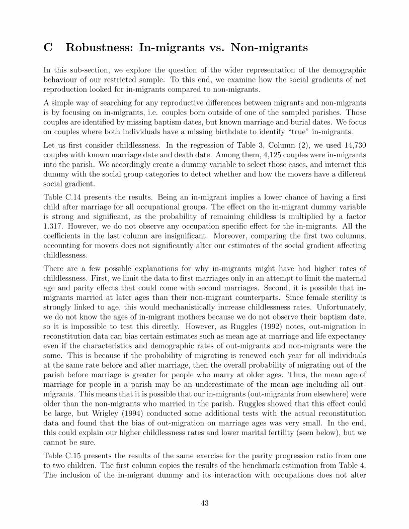
C Robustness: In-migrants vs. Non-migrants

In this sub-section, we explore the question of the wider representation of the demographicbehaviour of our restricted sample. To this end, we examine how the social gradients of netreproduction looked for in-migrants compared to non-migrants.

A simple way of searching for any reproductive differences between migrants and non-migrantsis by focusing on in-migrants, i.e. couples born outside of one of the sampled parishes. Thosecouples are identified by missing baptism dates, but known marriage and burial dates. We focuson couples where both individuals have a missing birthdate to identify “true” in-migrants.

Let us first consider childlessness. In the regression of Table 3, Column (2), we used 14,730couples with known marriage date and death date. Among them, 4,125 couples were in-migrantsinto the parish. We accordingly create a dummy variable to select those cases, and interact thisdummy with the social group categories to detect whether and how the movers have a differentsocial gradient.

Table C.14 presents the results. Being an in-migrant implies a lower chance of having a firstchild after marriage for all occupational groups. The effect on the in-migrant dummy variableis strong and significant, as the probability of remaining childless is multiplied by a factor1.317. However, we do not observe any occupation specific effect for the in-migrants. All thecoefficients in the last column are insignificant. Moreover, comparing the first two columns,accounting for movers does not significantly alter our estimates of the social gradient affectingchildlessness.

There are a few possible explanations for why in-migrants might have had higher rates ofchildlessness. First, we limit the data to first marriages only in an attempt to limit the maternalage and parity effects that could come with second marriages. Second, it is possible that in-migrants married at later ages than their non-migrant counterparts. Since female sterility isstrongly linked to age, this would mechanistically increase childlessness rates. Unfortunately,we do not know the ages of in-migrant mothers because we do not observe their baptism date,so it is impossible to test this directly. However, as Ruggles (1992) notes, out-migration inreconstitution data can bias certain estimates such as mean age at marriage and life expectancyeven if the characteristics and demographic rates of out-migrants and non-migrants were thesame. This is because if the probability of migrating is renewed each year for all individualsat the same rate before and after marriage, then the overall probability of migrating out of theparish before marriage is greater for people who marry at older ages. Thus, the mean age ofmarriage for people in a parish may be an underestimate of the mean age including all out-migrants. This means that it is possible that our in-migrants (out-migrants from elsewhere) wereolder than the non-migrants who married in the parish. Ruggles showed that this effect couldbe large, but Wrigley (1994) conducted some additional tests with the actual reconstitutiondata and found that the bias of out-migration on marriage ages was very small. In the end,this could explain our higher childlessness rates and lower marital fertility (seen below), but wecannot be sure.

Table C.15 presents the results of the same exercise for the parity progression ratio from oneto two children. The first column copies the results of the benchmark estimation from Table 4.The inclusion of the in-migrant dummy and its interaction with occupations does not alter

43

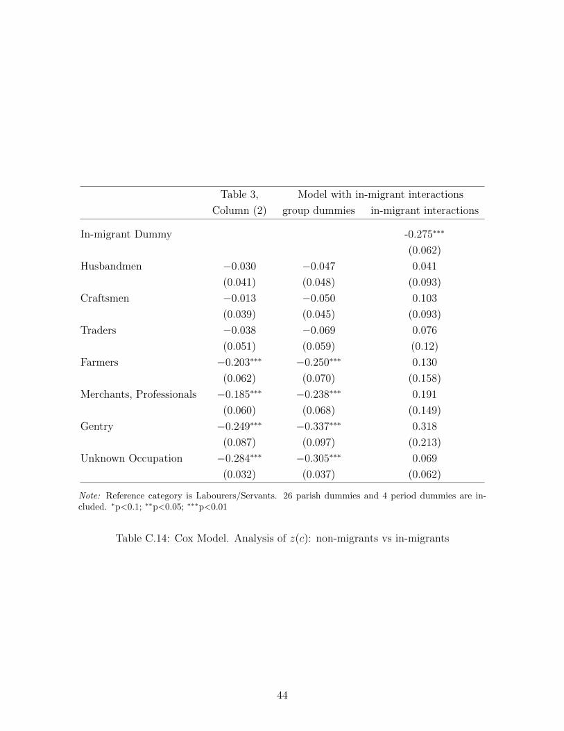
Table 3, Model with in-migrant interactions

Column (2) group dummies in-migrant interactions

In-migrant Dummy -0.275∗∗∗

(0.062)

Husbandmen −0.030 −0.047 0.041

(0.041) (0.048) (0.093)

Craftsmen −0.013 −0.050 0.103

(0.039) (0.045) (0.093)

Traders −0.038 −0.069 0.076

(0.051) (0.059) (0.12)

Farmers −0.203∗∗∗ −0.250∗∗∗ 0.130

(0.062) (0.070) (0.158)

Merchants, Professionals −0.185∗∗∗ −0.238∗∗∗ 0.191

(0.060) (0.068) (0.149)

Gentry −0.249∗∗∗ −0.337∗∗∗ 0.318

(0.087) (0.097) (0.213)

Unknown Occupation −0.284∗∗∗ −0.305∗∗∗ 0.069

(0.032) (0.037) (0.062)

Note: Reference category is Labourers/Servants. 26 parish dummies and 4 period dummies are in-cluded. ∗p<0.1; ∗∗p<0.05; ∗∗∗p<0.01

Table C.14: Cox Model. Analysis of z(c): non-migrants vs in-migrants

44

the estimation of the parity progression ratio for the non-migrants, as the results displayedthe second column are very close to those of the first column. However, in-migrants belongingto the gentry did experience a higher parity progression ratio than gentry non-migrants. Thecoefficient is strong and significant, but it is based on only 30 couples out of 151 belonging tothe Gentry who were in-migrants. Thus, it does not explain away our gradient.

The results for the progression to the next parity are presented in Table C.16. Here, in-migrantshave a lower chance of having a third child; their probability of having a third child is 83 percent of the one of the non-migrants. However, this does not depend on their occupation becauseall of the interaction terms are insignificant.

Table C.17 presents the results for the mortality rate of children under the age of 15. In-migrantshad moderately higher mortality levels for children, but there were no statistically significantdifferences between non-migrants and in-migrants of each specific social group. Thus, our socialgradient remain intact.

In conclusion, in-migrants were different from non-migrants as they were more likely to bechildless, had lower parity progression rates, and higher child mortality. This means that theiroverall net fertility was slightly lower than non-migrants. However, there is no significant socialgradient to these effects, so not accounting for migration does not seem to strongly influenceat least these three margins of reproductive success.

45

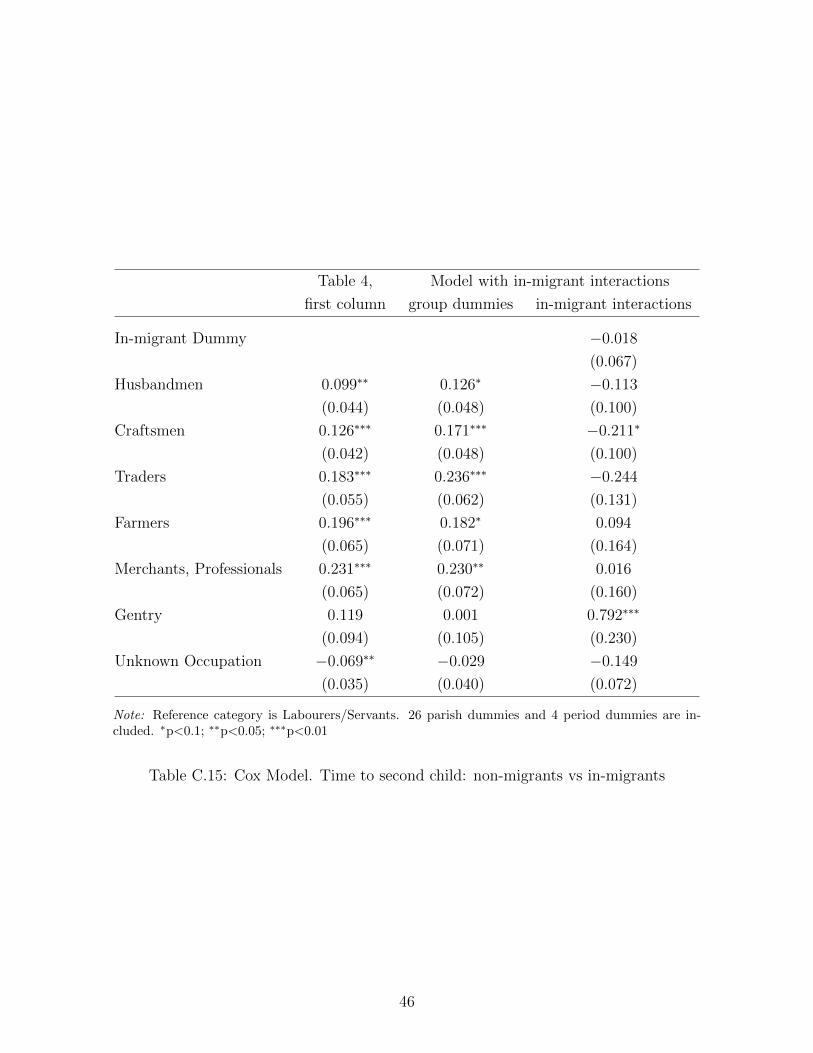
Table 4, Model with in-migrant interactions

first column group dummies in-migrant interactions

In-migrant Dummy −0.018

(0.067)

Husbandmen 0.099∗∗ 0.126∗ −0.113

(0.044) (0.048) (0.100)

Craftsmen 0.126∗∗∗ 0.171∗∗∗ −0.211∗

(0.042) (0.048) (0.100)

Traders 0.183∗∗∗ 0.236∗∗∗ −0.244

(0.055) (0.062) (0.131)

Farmers 0.196∗∗∗ 0.182∗ 0.094

(0.065) (0.071) (0.164)

Merchants, Professionals 0.231∗∗∗ 0.230∗∗ 0.016

(0.065) (0.072) (0.160)

Gentry 0.119 0.001 0.792∗∗∗

(0.094) (0.105) (0.230)

Unknown Occupation −0.069∗∗ −0.029 −0.149

(0.035) (0.040) (0.072)

Note: Reference category is Labourers/Servants. 26 parish dummies and 4 period dummies are in-cluded. ∗p<0.1; ∗∗p<0.05; ∗∗∗p<0.01

Table C.15: Cox Model. Time to second child: non-migrants vs in-migrants

46

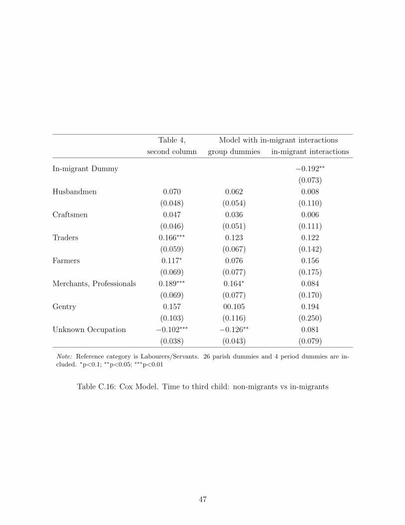
Table 4, Model with in-migrant interactions

second column group dummies in-migrant interactions

In-migrant Dummy −0.192∗∗

(0.073)

Husbandmen 0.070 0.062 0.008

(0.048) (0.054) (0.110)

Craftsmen 0.047 0.036 0.006

(0.046) (0.051) (0.111)

Traders 0.166∗∗∗ 0.123 0.122

(0.059) (0.067) (0.142)

Farmers 0.117∗ 0.076 0.156

(0.069) (0.077) (0.175)

Merchants, Professionals 0.189∗∗∗ 0.164∗ 0.084

(0.069) (0.077) (0.170)

Gentry 0.157 00.105 0.194

(0.103) (0.116) (0.250)

Unknown Occupation −0.102∗∗∗ −0.126∗∗ 0.081

(0.038) (0.043) (0.079)

Note: Reference category is Labourers/Servants. 26 parish dummies and 4 period dummies are in-cluded. ∗p<0.1; ∗∗p<0.05; ∗∗∗p<0.01

Table C.16: Cox Model. Time to third child: non-migrants vs in-migrants

47

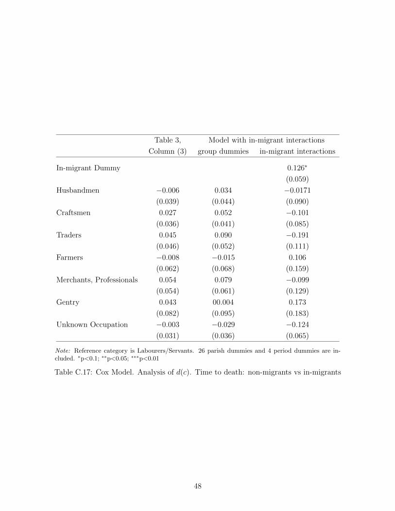
Table 3, Model with in-migrant interactions

Column (3) group dummies in-migrant interactions

In-migrant Dummy 0.126∗

(0.059)

Husbandmen −0.006 0.034 −0.0171

(0.039) (0.044) (0.090)

Craftsmen 0.027 0.052 −0.101

(0.036) (0.041) (0.085)

Traders 0.045 0.090 −0.191

(0.046) (0.052) (0.111)

Farmers −0.008 −0.015 0.106

(0.062) (0.068) (0.159)

Merchants, Professionals 0.054 0.079 −0.099

(0.054) (0.061) (0.129)

Gentry 0.043 00.004 0.173

(0.082) (0.095) (0.183)

Unknown Occupation −0.003 −0.029 −0.124

(0.031) (0.036) (0.065)

Note: Reference category is Labourers/Servants. 26 parish dummies and 4 period dummies are in-cluded. ∗p<0.1; ∗∗p<0.05; ∗∗∗p<0.01

Table C.17: Cox Model. Analysis of d(c). Time to death: non-migrants vs in-migrants

48

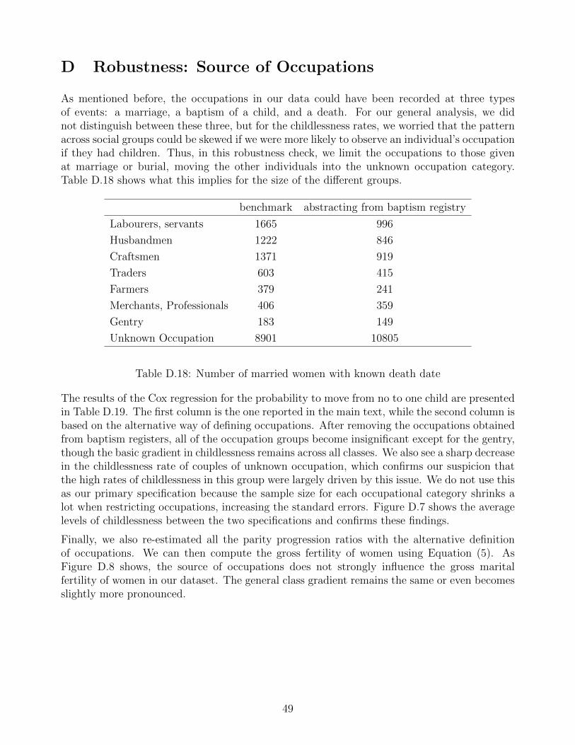
D Robustness: Source of Occupations

As mentioned before, the occupations in our data could have been recorded at three typesof events: a marriage, a baptism of a child, and a death. For our general analysis, we didnot distinguish between these three, but for the childlessness rates, we worried that the patternacross social groups could be skewed if we were more likely to observe an individual’s occupationif they had children. Thus, in this robustness check, we limit the occupations to those givenat marriage or burial, moving the other individuals into the unknown occupation category.Table D.18 shows what this implies for the size of the different groups.

benchmark abstracting from baptism registry

Labourers, servants 1665 996

Husbandmen 1222 846

Craftsmen 1371 919

Traders 603 415

Farmers 379 241

Merchants, Professionals 406 359

Gentry 183 149

Unknown Occupation 8901 10805

Table D.18: Number of married women with known death date

The results of the Cox regression for the probability to move from no to one child are presentedin Table D.19. The first column is the one reported in the main text, while the second column isbased on the alternative way of defining occupations. After removing the occupations obtainedfrom baptism registers, all of the occupation groups become insignificant except for the gentry,though the basic gradient in childlessness remains across all classes. We also see a sharp decreasein the childlessness rate of couples of unknown occupation, which confirms our suspicion thatthe high rates of childlessness in this group were largely driven by this issue. We do not use thisas our primary specification because the sample size for each occupational category shrinks alot when restricting occupations, increasing the standard errors. Figure D.7 shows the averagelevels of childlessness between the two specifications and confirms these findings.

Finally, we also re-estimated all the parity progression ratios with the alternative definitionof occupations. We can then compute the gross fertility of women using Equation (5). AsFigure D.8 shows, the source of occupations does not strongly influence the gross maritalfertility of women in our dataset. The general class gradient remains the same or even becomesslightly more pronounced.

49

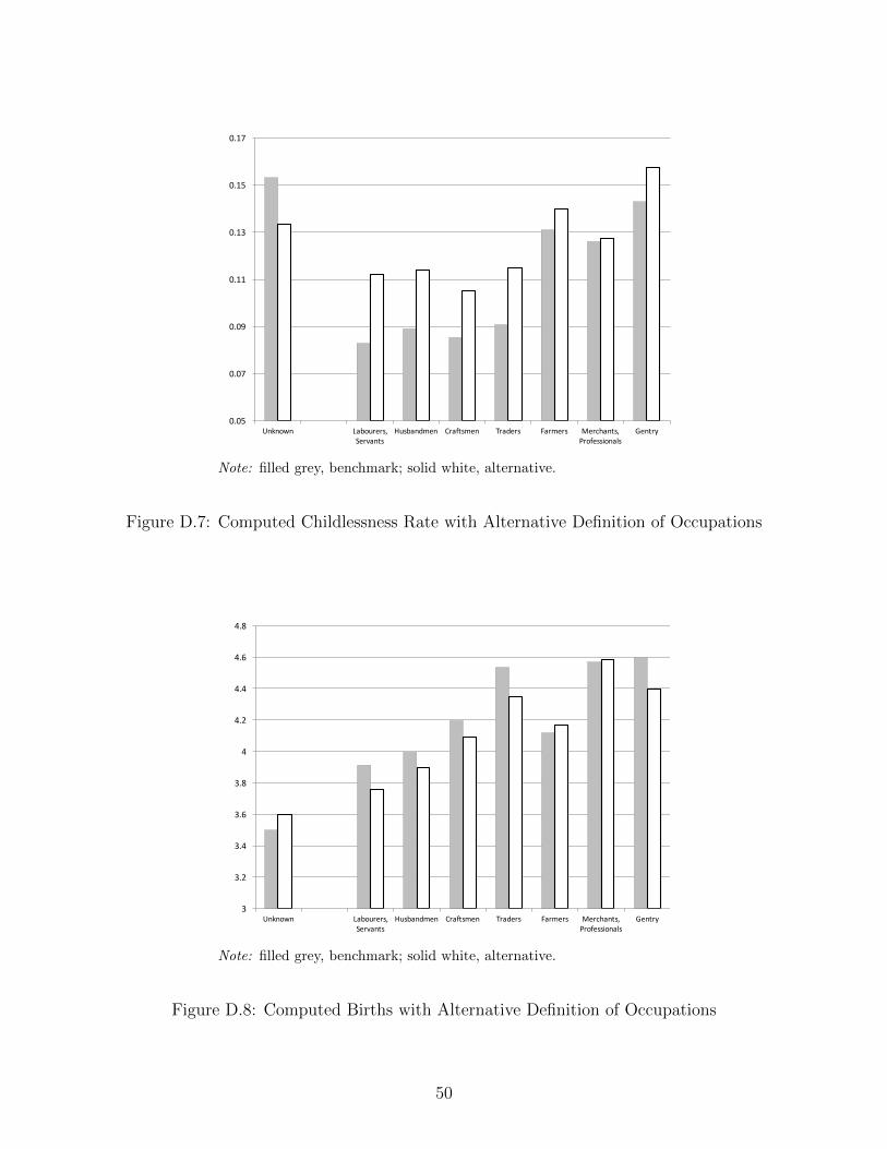
0.05

0.07

0.09

0.11

0.13

0.15

0.17

Unknown Labourers,Servants

Husbandmen Craftsmen Traders Farmers Merchants,Professionals

Gentry

Note: filled grey, benchmark; solid white, alternative.

Figure D.7: Computed Childlessness Rate with Alternative Definition of Occupations

3

3.2

3.4

3.6

3.8

4

4.2

4.4

4.6

4.8

Unknown Labourers,Servants

Husbandmen Craftsmen Traders Farmers Merchants,Professionals

Gentry

Note: filled grey, benchmark; solid white, alternative.

Figure D.8: Computed Births with Alternative Definition of Occupations

50

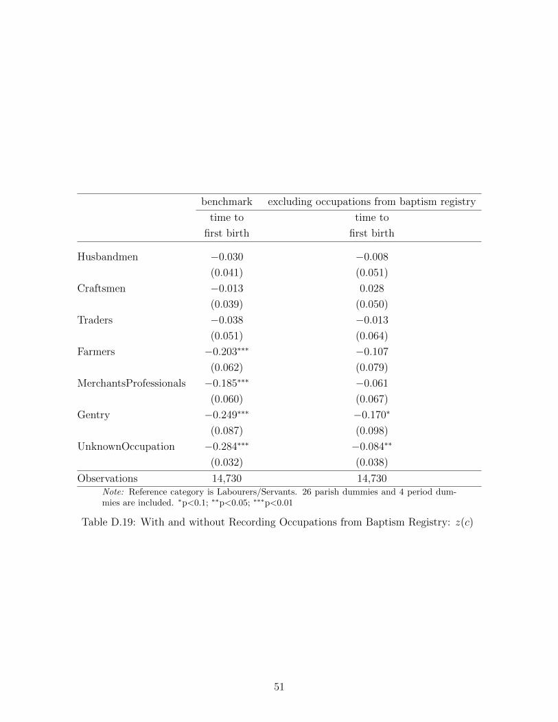
benchmark excluding occupations from baptism registry

time to time to

first birth first birth

Husbandmen −0.030 −0.008

(0.041) (0.051)

Craftsmen −0.013 0.028

(0.039) (0.050)

Traders −0.038 −0.013

(0.051) (0.064)

Farmers −0.203∗∗∗ −0.107

(0.062) (0.079)

MerchantsProfessionals −0.185∗∗∗ −0.061

(0.060) (0.067)

Gentry −0.249∗∗∗ −0.170∗

(0.087) (0.098)

UnknownOccupation −0.284∗∗∗ −0.084∗∗

(0.032) (0.038)

Observations 14,730 14,730Note: Reference category is Labourers/Servants. 26 parish dummies and 4 period dum-mies are included. ∗p<0.1; ∗∗p<0.05; ∗∗∗p<0.01

Table D.19: With and without Recording Occupations from Baptism Registry: z(c)

51

ISSN 1379-244X D/2017/3082/1