Data Structures and Graph Algorithms Weighted Matchingsmehlhorn/ftp/WeightedMatchings.pdf · MPI Informatik 1 Kurt Mehlhorn Data Structures and Graph Algorithms Weighted Matchings

MPI Informatik 1 Kurt Mehlhorn

Data Structures and Graph Algorithms

Weighted Matchings

Kurt Mehlhorn and Guido Schafer

Max-Planck-Institut fur Informatik

K. Mehlhorn and G. Schafer: Implementation of O nmlogn Weighted Matchings in General

Graphs: The Power of Data Structures, Workshop on Algorithm Engineering (WAE), LNCS 1982,

23–38, full version to appear in Journal of Experimental Algorithmics

K. Mehlhorn and G. Schafer: A Heuristic for Dijkstra’s Algorithm with Many Targets and its Use

in Weighted Matching Algorithms, ESA 2001, LNCS 2161, 242–253,


Contents

1. the worst case running time of many graph algorithms can be considerably improved

by clever data structures (n number of nodes, m number of edges)

priority queues for shortest paths O n2 O m n logn

dynamic trees for maximum flows O n2 m O nm

mergeable p-queues for weighted matchings O n3 O nm logn

2. do these asymptotic improvements lead to improved “actual” running times ?

priority queues for Dijkstra’s shortest path algorithm

dynamic trees for maximum flow algorithms

mergeable priority queues for general weighted matchings ???

3. can we explain our experimental findings ???

4. today’s talk is an engineering talk and not a theory talk


Worst Case Analysis of Graph Algorithms vs Actual Running Times view execution as a sequence of basic operations, for example

– scan all edges incident to a node

– find a node with with minimal priority

derive an upper bound ai on the number of operations of type i

argue how operations of type i can be implemented and derive a time bound Ti

state ∑i aiTi as an upper bound on the running time

ai and Ti are stated as functions of n and m (number of nodes and edges, resp.) and

we are interested in the asymptotics

theoretical bottlenecks = the i’s such that aiTi determines the asymptotics

ai and Ti are upper bounds

ti = typical number of operations of type i

actual bottleneck = the i’s such that tiTi determines the running time


The Weighted Matching Problem G V E graph, W : E , edge costs

matching M = set of edges no two of which share an endpoint

M is perfect iff every node of G is matched

weight of a matching w M ∑e M w e

weighted matching problem

– compute perfect M with maximum (minimum) weight

– compute M with maximum (minimum) weight

– problems are reducible to each other (but it is better to solve them directly)

3 8

7 0

0 7

7 0

5

7

14

5

7

14


Algorithms Edmonds (65) gave blossom-shrinking alg, running time O n2m

Lawler (76) and Gabow (74) improved time to O n3

Galil, Micali, and Gabow (86) improved further to O nm logn

Gabow (90) improved further to O nm n2 logn .

underlying strategy is the same, algs use different data structures

– Edmonds, Lawler, Gabow only require arrays and lists

– Galil, Micali, and Gabow require mergeable and splitable priority queues

– Gabow (90) requires even more sophisticated data structures

Question: Is is worth using sophisticated data structures?


Implementations Applegate/Cook (93) and Cook/Rohe (97): Blossom IV

– implement O n3 algorithm

– refined by several powerful heuristics: jump start, multiple trees, variable δ,

pricing for complete geometric instances

– argue convincingly that their implementation is best

Mehlhorn/Schafer (00 + 01)

– implement variant of O nm logn algorithm

– use mergeable and splitable priority queue

– refined by some heuristics: multiple trees and improved jump start

– weighted matchings or weighted perfect matchings

– is usually faster than Blossom IV (except for dense geometric instances)

data structures make the worst case and the common case faster

– available as part of LEDA and built on top of LEDA


Some Timings

Delaunay Graphs

n B4 MS

10000 2.69 4.88

40000 17.60 21.68

160000 138.29 98.13

Sweep Triangulations

n B4 MS

10000 9.89 5.16

40000 95.96 24.09

160000 2373.18 121.99

Delaunay graphs and sweep triangulations are planar graphs

Delaunay Graphs are simpler than general triangulations

MS seems to have better asymptotics on these examples

– quadrupling n increases running time by factor 5 for MS

– and by factor 7 and more for B4.


More Timings random graphs, n 104, m 4n, random edge weights in 1 b

b B4 MS

1 3.99 0.85

100 3.10 2.58

10000 11.91 2.78

running time of MS depends less on range of edge weights and is faster in the

unweighted case

random graphs , n 4 104, m 6n

n B4 MS

best ave worst best ave worst

40000 49.02 55.15 60.74 9.93 10.30 11.09

running time of MS shows less variance


More Timings a chain with 2n vertices and 2n 1 edges. Edge weights are alternately 0 and 2 with

the extreme edges having weight 0.

heuristics construct matching consisting of the weight 2 edges,

one augmentation is needed to change the matching into a max-weight perfect

matching

n B4 MS

10000 94.75 0.25

20000 466.86 0.64

40000 2151.33 2.08

– running time of B4 grows quadratically

– running time of MS slightly more than

linearly

a graph provided to us by Cook and Rohe: n 151780 m 881317

B4 MS

200810.35 5993.61


Optimality Condition: The Bipartite Case

Lemma 1 A perfect matching M is optimal iff there are node potentials yu u V with

yu yv wuv for all uv E

yu yv wuv for all uv M

Let N be any other perfect matching. Then

w N ∑e N

we ∑u A

yu ∑v B

yv ∑e M

we w M

reduced cost of edge uv πuv yu yv wuv

an edge is called tight, if its reduced cost is equal to 0.

A High-Level View of Edmonds’ Algorithm maintains a matching M and node potentials yu u V

– reduced edge costs are non-negative: πuv yu yv wuv 0

– edges in M are tight: πuv 0 for uv M

operates in phases; in each phase M is increased by one

a phase consists of subphases

– trees of tight edges rooted at free nodes are grown with the goal of finding an

augmenting path connecting two free nodes 0 2 0 2 020 0 2 0 2

– (subphase) when tree growing process stops, dual variables are changed to make

more edges tight and hence to allow further growth

– when augmenting path is found, M is increased and phase ends.

tree growing process may stop Ω n times and dual variable update may require to

change Ω n potentials with primitive data structures: time Ω n2 per phase

priority queues reduce cost of dual update to O logn time O m logn per phase


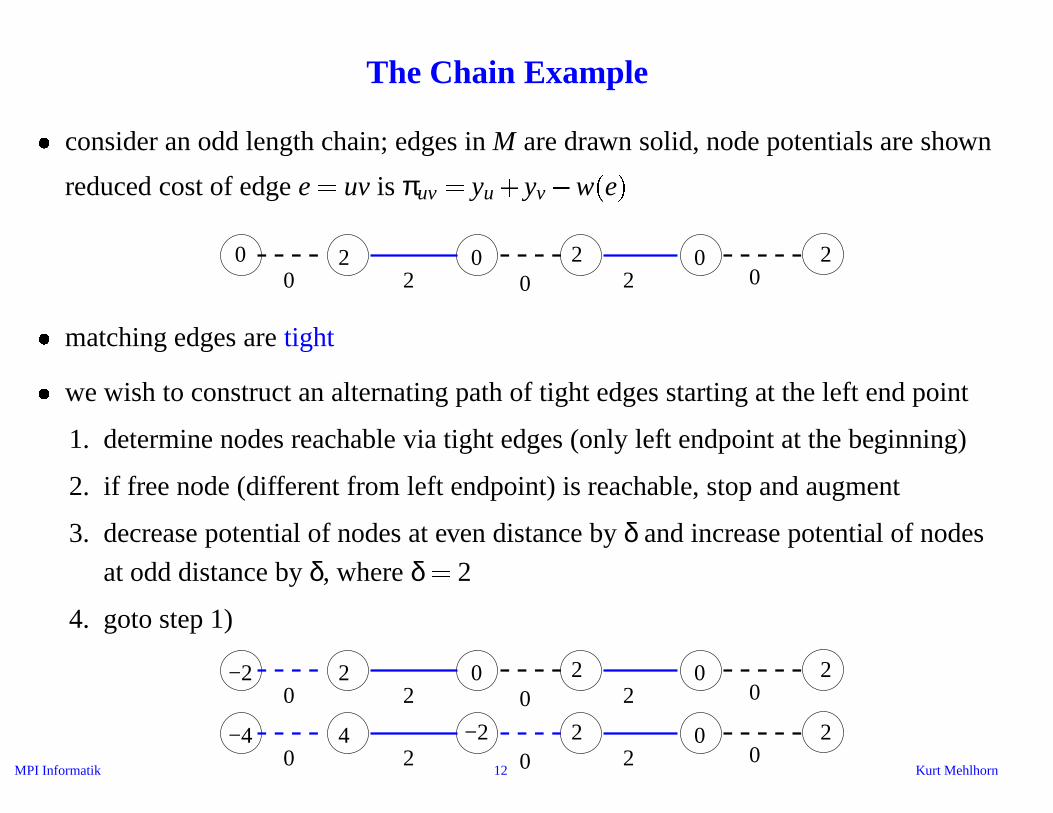
The Chain Example consider an odd length chain; edges in M are drawn solid, node potentials are shown

reduced cost of edge e uv is πuv yu yv w e

0 2 0 2 020 0 2 0 2

matching edges are tight

we wish to construct an alternating path of tight edges starting at the left end point

1. determine nodes reachable via tight edges (only left endpoint at the beginning)

2. if free node (different from left endpoint) is reachable, stop and augment

3. decrease potential of nodes at even distance by δ and increase potential of nodes

at odd distance by δ, where δ 2

4. goto step 1)

0 2 0 2 02 0 2 0 2−2

0 2 0 2 02 0 2−4 4 −2


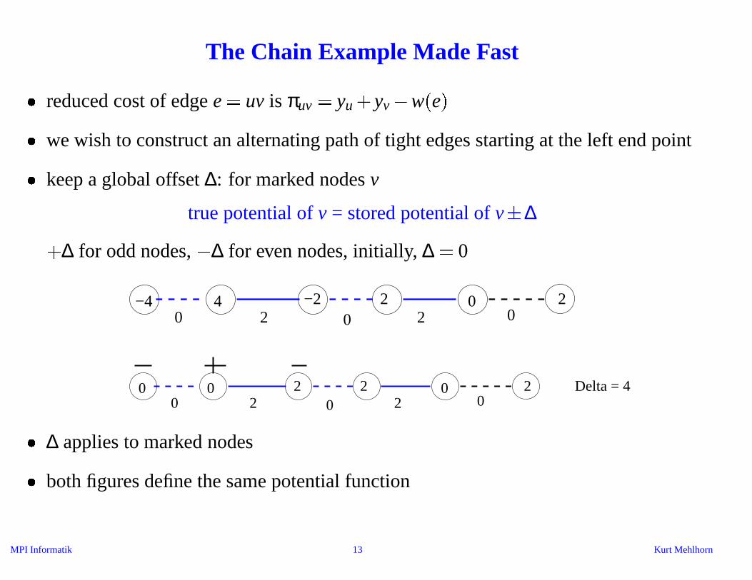
The Chain Example Made Fast reduced cost of edge e uv is πuv yu yv w e

we wish to construct an alternating path of tight edges starting at the left end point

keep a global offset ∆: for marked nodes v

true potential of v = stored potential of v ∆

∆ for odd nodes, ∆ for even nodes, initially, ∆ 0

0 2 0 2 02 0 2−4 4 −2

0 2 0 2 02 0 2 Delta = 4 0 0 2

∆ applies to marked nodes

both figures define the same potential function

The Chain Example Made Fast II keep a global offset ∆: for a node v reachable from left endpoint via tight edges

true potential of v = stored potential of v ∆

∆ for odd nodes, ∆ for even nodes, initially, ∆ 0

0 2 0 2 02 0 2 Delta = 4 0 0 2

∆ applies to marked nodes

new nodes are reachable via tight edges, we set their stored potential and mark them

0 2 0 2 0 0 0 2 4 2 Delta = 4−2

we change ∆ so as to make one more edge tight: ∆ ∆ δ, where δ 2

0 2 0 2 0 0 0 2 4 2−2 Delta = 6

potential update in time O 1


Profiling Data B4 spends most of its time in potential updates and work triggered by it

potential updates are not only theoretical bottleneck, they are the actual bottleneck

for the n3 algorithms

offset trick allows us to change the potential of many nodes with a few instructions

data structures keep the cost of other basic operations low

– determining δ and determining new tight edges

the following table gives numbers for sweep-triangulations, n 40000

dual adjustments node updates shrinks expands time

B4 12466 1179070 4913 433 23.41

MS 15812 7058 1766 21.98

B4 22488 11353087 10585 967 278.25

MS 24505 12140 2573 26.05

we cannot use the variable δ-heuristic of BIV


More Details: Alternating Trees in Bipartite Case trees are rooted at free nodes and tree edges are tight

vertices on even levels are reached via matching

edges, vertices on odd levels are reached via non-

matching edges

action if there is tight edge v w with v even

– w is in no tree grow tree, i.e.,

add w and its mate to the tree

– w is even and in different tree: breakthrough

– w is odd: do nothing

$v$

O E O EE

$v$ $w$ $\mathitmate(w)$

E O E O E

if there is no such edge: potential change by δ, where

δ min reduced cost of any edge connecting a non-tree node with an even tree node


Priority Queues

maintain a set of priorities, under the following operations

create an empty priority queue

insert a priority

delete a priority (given by a pointer to its position in the data structures)

extract minimum priority

decrease a priority (given by a pointer to its position in the data structures)

there are priority queue implementations supporting all operations in logarithmic

time

even time O 1 for decrease p


Usage of Priority Queues: Bipartite Case δ min reduced cost of any edge connecting a non-tree node with an even tree node

for every non-tree node v keep

min cost v = minimum reduced cost of any edge connecting v to an even tree node

keep all min cost-values in a priority queue

tree growing and dual updates

– extract min determines δ and the node to be added to the tree

– delete new tree nodes from the priority queue

– update priorities of remaining non-tree nodes by scanning the edges incident to

the new even tree node u

– for every such edge uv check min cost v and decrase if necessary

– after dual update, tree will grow by at least two nodes and hence there are at most

n 2 dual updates per phase

– cost of one dual update = 1 extract min + deg u decrease p

– total cost of dual updates per phase = O n logn m


An Optimization (ESA 01) grow a single tree

“conceptually” combine all free non-tree nodes into a single node and use them to

derive a threshold for pq-operations

three additional lines of code

considerably reduces number of queue operations

about halves the running time

Lemma 2 (MS, ESA 01) On random graphs with average outdegree c the fraction of

saved queue operations is at least

1 2 lncc

For example, for c 8, at least 49% of the queue operations are saved, and

for c 16, at least 70% are saved.


Lemma 3 (Optimality Conditions for the General Case)A perfect matching M is optimal iff there are node potentials yu u V and odd set

potentials zB B O with

zB 0 for all B O,

πuv yu yv wuv ∑uv B zB 0 for all uv E

πuv 0 for all uv M (matching edges are tight)

sets B with zB 0 form a nested family and are full, i.e., exactly one node has mate

outside B and there are B 2 matching edges inside.

Let N be any other perfect matching. Then

w M ∑e M

we ∑u V

yu ∑uv M

∑B ;uv B

zB

∑u V

yu ∑B ;zB 0

zB B 2

∑u V

yu ∑uv N

∑B ;uv B

zB ∑e N

we w N


Edmonds’ Algorithm: More Details alg maintains a matching M and dual variables yv, zB

all edges have non-negative reduced cost

matching edges are tight

init: M /0, zB 0 for all B , yv maxe E we

sets B with zB 0 are called blossoms and form a

nested family of full sets

surface blossom = maximal blossom

vertices of current graph =– nodes of original graph outside blossoms

– surface blossoms

surface blossoms are matched in current graph

free vertices are original nodes

alg grows alternating trees rooted at free vertices


Alternating Trees all edges in the tree are tight

vertices on even levels are reached via matching

edges, vertices on odd levels are reached via non-

matching edges

actions if there is tight edge v w with v even

– w is in no tree: add w and its mate

w and/or its mate may be surface blossoms

– w is even and in different tree: breakthrough

– w is even and in same tree: new even blossom

– w is odd: do nothing

$v$

O E O EE

$v$ $w$ $\mathitmate(w)$

E O E O E

$v$ $w$$w$

$b$ $v$$u$


Dual Updates I when tree growing process stops without a breakthrough, update the duals

goal is to make edges tight that connect non-tree nodes with even tree nodes

yv yv δ for even nodes, yv yv δ for odd nodes

zB zB 2δ for even surface blossoms, zB zB 2δ for odd surface blossoms

does not change the reduced cost of any edge

– inside a blossom or in alternating trees

decreases the reduced cost of edges between non-tree nodes and even tree nodes, and

between even tree nodes and the potential of odd surface blossoms

constraints on δ– δ δ1 min πuv ; u even, v non-tree !

– δ δ2 min πuv 2 ; u and v even !

– δ δ3 min zB 2 ; B is an odd surface blossom !– choose δ min δ1 δ2 δ3 .


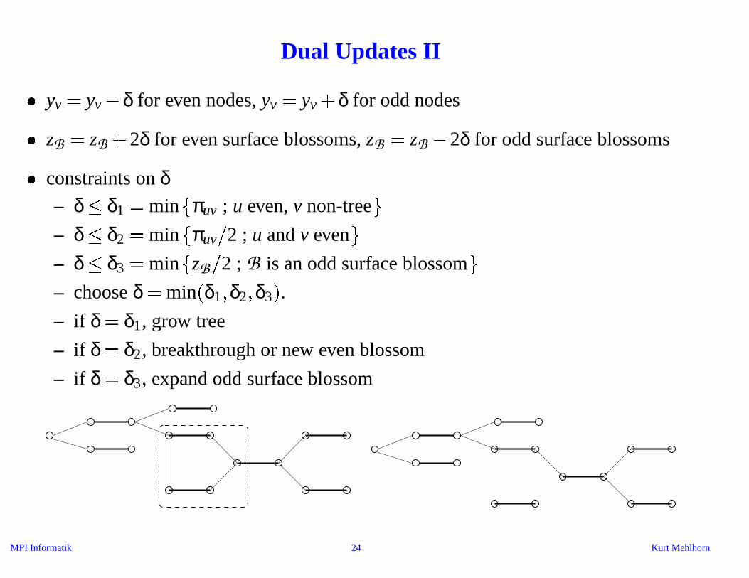
Dual Updates II yv yv δ for even nodes, yv yv δ for odd nodes

zB zB 2δ for even surface blossoms, zB zB 2δ for odd surface blossoms

constraints on δ– δ δ1 min πuv ; u even, v non-tree !

– δ δ2 min πuv 2 ; u and v even !

– δ δ3 min zB 2 ; B is an odd surface blossom !

– choose δ min δ1 δ2 δ3 .

– if δ δ1, grow tree

– if δ δ2, breakthrough or new even blossom

– if δ δ3, expand odd surface blossom


Mergeable and Splitable Priority Queues priority queues are needed to keep track of various δ’s

mergeable and splitable priority queues

– priorities are associated with elements of sequences

– have a priority queue for each sequence

– sequences can be concatenated and split

edges from A to even tree nodes must be considered in first and last figure, but not in

the middle figure

two non−tree blossoms

grow treeodd even

expand odd blossom

two non−tree blossomsA

A

A


Summary and Open Problems have carefully implemented variant of O nm logn algorithm

a significant practical contribution, a small theoretical advance

– first implementation of the algorithm

– simplified treatment of reduced costs

– optimization for bipartite graphs, analysis thereof

new impl is superior to previous ones

impl is based on LEDA and would have been impossible without

how about Gabow’s O nm n2 logn alg?

design families of problem instances which force algs into their worst case

transfer optimization from bipartite graphs to general graphs

explain asymptotic behavior on Delaunay graphs, sparse random graph

Documents

Data Structures and Graph Algorithms Weighted Matchingsmehlhorn/ftp/WeightedMatchings.pdf · MPI Informatik 1 Kurt Mehlhorn Data Structures and Graph Algorithms Weighted Matchings