Data-parallel numerical methods in a weather forecast model

ELSEVIER Applied Numerical Mathematics 19 (1995) 159-171 MATHEMATICS

Data-parallel numerical methods in a weather forecast model

Lex Wolters a,*,l, Gera rd Cats b,l,2, Nils Gus ta f sson c'l'3, Tomas Wi lhe lmsson d,4

a High Performance Computing Division, Department of Computer Science, Leiden University, P.O. Box 9512, 2300 RA Leiden, Netherlands

Royal Netherlands Meteorological Institute, P.O. Box 201, 3730 AE De Bilt, Netherlands c Swedish Meteorological and Hydrological Institute, S-60176 Norrk~ping, Sweden

d NADA, Royal Institute o f Technology, Stockholm, Sweden

Abstract

The results presented in this paper are part of a research project to investigate the possibilities to apply massively parallel architectures for numerical weather forecasting. Within numerical weather forecasting several numerical techniques are used to solve the model equations. This paper compares the performance of implementations on a MasPar system of two techniques, finite difference and spectral, that are adopted in the numerical weather forecasting model HIRLAM. The operational HIRLAM model is based on finite difference methods, while the spectral model is still in a research phase. Also the differences in relative performance of these methods on the MasPar and vector architectures will be discussed.

1. Introduction

The HIRLAM (High Resolution Limited Area Modeling) forecasting system has been developed within a common research project among the weather services of Denmark, Finland, Iceland, Ireland, the Netherlands, Norway, and Sweden [12,6]. The application of this forecasting system requires significant computing power. Present operational applications of the HIRLAM system are using super- or minisuper-computers including vector processors and a moderate degree of parallelism (2-8 processors). The forecasting model has also been applied in research mode on high end workstations.

* Corresponding author. Support was provided by the Esprit Agency EC-DGIII under Grant No. APPARC 6634 BRA Ill. E-mail: [email protected].

J Support was provided through the Human Capital and Mobility Programme of the European Community. 2 E-mail: [email protected]. 3 E-mail: [email protected]. 4 E-mail: [email protected].

0168-9274/95/$09.50 (~ 1995 Elsevier Science B.V. All rights reserved SSDI 01 68-9274( 95)00023-2

160 L. Wolters et al./Applied Numerical Mathematics 19 (1995) 159-171

To be able to simulate and forecast weather developments with more details, it is of general interest to apply the model with increased spatial resolutions. Present operational implementations can describe scales of motion of the order of 50-100 km while there is a need to move towards descriptions of spatial scales of the order of a few kilometers. The needed computer power for such resolutions, together with the general parallel structure of the weather prediction problem, makes it interesting to apply the HIRLAM model on massively parallel architectures.

In this paper the performances of different numerical methods within the HIRLAM forecast model on a massively parallel platform are compared. Also the performance differences compared to a vector architecture are discussed. In Section 2 a short overview of the HIRLAM model and its equations is given. Section 3 describes the numerical methods and their impact on the parallelization of the model. The MasPar hardware and software are presented in Section 4. The parallelization strategy is briefly outlined in Section 5. Performance results are shown and discussed in Section 6. Section 7 finishes with some concluding remarks.

2. HIRLAM

A modem atmospheric model such as HIRLAM, consists of two main parts. The first is called the "dynamics"; its task is to solve the basic model equations. The second part is called the "physics"; it describes the aggregate effect of the physical processes with scales smaller than the model resolution, on the larger, resolved, scales. Some physical processes like radiation, not directly described by the basic model equations, are also parameterized.

The basic set of equations in a atmospheric circulation model consists of a set of three-dimensional coupled nonlinear hyperbolic partial differential equations (PDEs). They are solved in the dynamics part of the model. The equations are known as the Primitive Equations, and can be derived from the Navier-Stokes equations (see e.g. [7] ). The equations describe five prognostic variables: two horizontal wind components u and v, the temperature T, the specific humidity q, and the surface pressure Ps.

In the HIRLAM forecast model [10] the prognostic variables are computed on a spherical horizontal coordinate system with longitude A and latitude 0. The vertical coordinate r/(p, Ps) is hybrid between pressure based and terrain following coordinates with r/(0, p.,) --0 and r/(ps, ps) = 1.

Within this coordinate system the primitive equations can be expressed as • two horizontal momentum equations:

au au RdTv 0 lnp 1 0 -~ ( f + ( ) v - " (1 = ~a~ acosO Oa acosOOa ( ¢ + E ) + P " + K ~ " )

ego OV RdTv 0 lnp 1 0 - - -- - ( f + sC)u - / / (~b + E) + Pv + Kv; (2) at Or/ a O0 a 00

• the hydrostatic equation (which is basically an approximated form of the vertical momentum equation):

R Lap. (3) O~ p 0~'

L. Wolters et al. /Applied Numerical Mathematics 19 (1995) 159-171 161

• the thermodynamic equation:

3T u 37"

?t a cos 0 3A

• the moisture equation:

3q u 3q

3t a cos 0 3/l

• the continuity equation:

v 3T

a 30

3T xTjo

//3-~ + (1 + ( 8 - 1 ) q ) p + Pr + KT; (4)

v aq .3q aOO ~7--~ -4- Pq A- Kq; (5)

3---~ ot + V " v h + ~-~ ¢! =0. (6)

In these equations we have the geopotential & (= gz) , the Coriolis parameter f - - 2 ~ s i n 0 , the earth angular velocity .O, the earth radius a, and the virtual temperature Tv = (1 + (e -1 - l )q )T . In this last formula e = Ra/Rv, where Rd is the gas constant for dry air and Rv is the gas constant for water vapor. Furthermore, K -- Ra/Cpd with Cad the specific heat for dry air at constant pressure, and to is the pressure vertical velocity (dp /d t ) , which is evaluated by vertical integration of the continuity equation (see [10] ). The symbol 8 denotes Cp~/Cpd with C w, the specific heat for moist air at constant pressure. Also

acosO 3A [cosOu] and E = ~ ( u 2 + v 2).

Finally, Px is the tendency for variable X from (vertical) parameterized processes calculated by the physics part of the model, and the term Kx describes the tendency for variable X from horizontal turbulent mixing, which is called horizontal diffusion (see Section 3).

3. Numerical methods

As mentioned in Section 2 the dynamics part of HIRLAM solves Eqs. ( 1 ) - ( 6 ) . The solution can be obtained by several numerical methods. Firstly, it is possible to choose between a gridpoint (finite difference) method or a spectral method. These methods will be discussed in Sections 3.1 and 3.2. A second option is based on the difference in numerical stability between explicit and implicit methods. This will be discussed in Section 3.3. The third option describes the atmosphere in a semi-Lagrangian formulation instead of an Eulerian representation. It is still in a research phase, and will not be addressed in this paper.

The terms Px in Eqs. ( 1 ) - ( 6 ) are calculated by the physics part of HIRLAM. It contains routines for integration and filtering algorithms, etc. Almost all physical processes take place in the vertical direction without any horizontal dependencies. Therefore the parallelization of this part of the model is trivial, if the required data in the vertical column of each horizontal datapoint are stored in the memory of one processor.

Horizontal diffusion is considered to be part of the dynamics (the terms Kx in Eqs. ( 1 ) - ( 6 ) ) . Due to horizontal advection and physical parameterization schemes aliasing effects have a tendency to accumulate energy on the shortest resolvable wave lengths. In numerical forecast models this effect

162 L. Wolters et al. / Applied Numerical Mathematics 19 (1995) 159-171

is called nonlinear instability and it must be controlled by the so-called horizontal diffusion (or filtering) that removes energy from the shortest wave lengths.

An important and critical part of any limited area model is the adoption of the model variables along the horizontal boundaries to externally given boundary conditions provided by e.g. a global forecast model. In the present HIRLAM model this adoption is carried out by relaxation towards the boundary conditions in a boundary relaxation zone [9]. Full weights (-- 1.0) are given to the external boundary values along the outer boundary of the boundary relaxation zone. Zero weights (-- 0) are given along the inner boundary of the boundary relaxation zone.

In the following subsections we will describe each numerical method within the HIRLAM dynamics in more detail. In particular the resulting type of communication on a parallel system will be presented. The flow of computations for each method is also shown.

3.1. Gridpoint version

The gridpoint version [10] of HIRLAM is used operationally by several weather services. It is based on finite difference methods. As an illustration we consider the simple example of the one-dimensional advection of temperature. In analytic form one has

aT aT -- u-:- (7) a--~

dX

with temperature T and wind component u in the x-direction at time t. In the most simple form (a nonstaggered horizontal grid) the discrete gridpoint version with a leap-frog time-stepping results in

At T ( x , t q- At) ~- T ( x , t - At) q- --;--u(x, t) ( T ( x -t- Ax, t) - T ( x - Ax, t) ) ,

lAX (8)

where T ( x , t) is the temperature in gridpoint x at time t, u(x , t) is the wind component in the x-direction in gridpoint x at time t, At is the time step, and Ax is the grid distance in the x-direction.

In the HIRLAM model a more complex discretization is implemented. The variables are defined and calculated on a staggered grid. In the horizontal plane this is the so-called Arakawa C-grid [2], which is shown in Fig. 1 (a). In Fig. 1 (b) the vertical structure is presented. As time discretization the well-known leap-frog method is implemented in the HIRLAM model.

In the fully explicit gridpoint version of HIRLAM the following calculations are carried out during one time step with the assumption that the values of the variables at time t and t - At are available:

(1) Compute the explicit dynamical tendencies at time t. (2) Compute the physical tendencies at time t - At. Some of the parameterization schemes also

use dynamical tendencies to derive values valid at time t + At. (3) Compute the horizontal diffusion tendencies at time t - At. (4) Perform a leap-frog time step and apply a time filter to obtain new values at time t + At and

t. The time filter suppresses any discrepancies between odd and even time steps due to the leap-frog scheme.

Concerning the parallelization of the example given by Eq. (8) it can be seen that only nearest neighbor communications are required, since the new value of the variable T depends only on values of neighboring gridpoints. This holds also for the gridpoint version of HIRLAM in general.

L. Wolters et al./ Applied Numerical Mathematics 19 (1995) 159-171 163

Ps T

q t I

v _ _ +

I

P.~ T lu q': i

I U - - - - - J [ -

I P., T l u

• A X ,

u Ps T u Ps T I q I

- I - - - - -

I

lu Ps I q

I

I lu Ps

q

U

Ps T q

U

P.~ 7" T q q q

(a)

T Ay

B-value Level number Model variables i ~ - - 0 - 0 . 0

- 1 T , q , u , v I - 1~ il

- 2 T , q , u , v

- 2½ i 7

1 - NLEV 2 ~/

- NLEV T, q, u, v I ~, 1.0 NLEV + g ~/= 0, p.~

, 7 / / / / / / / / / / / / / / / / / / / / / / / / / / / / / / / /

(b) Fig. 1. The horizontal (a) and vertical (b) discrete grid in the HIRLAM model.

3.2. Spectral version

The spectral version is based on solving the primitive equations by a spectral transform technique [4,15]. These transforms require periodic boundary conditions. This is straightforward for a global geometry, since this geometry allows for a natural periodic variation of all variables in both directions. To introduce this technique in a limited area model initial steps were taken by Haugen and Machenhauer [ 8 ], who developed a spectral limited area shallow water model based on the idea of extending the limited area in the two horizontal dimensions in order to obtain periodicity in these two dimensions and to permit the use of efficient fast Fourier transforms. The same idea has been implemented by Gustafsson [ 5 ] into the full multi-level HIRLAM framework. The geometry of using an extension zone to obtain periodic variations in both horizontal dimensions of the forecast model variables is illustrated in Fig. 2.

To apply the spectral transform technique for Eq. (7) one will start the integrations from spectral coefficients 7~ and 12, defined by e.g.

T ( x , t ) = 1 ~-~7"(k,t) exp( ikx) , (9)

T(k , t) = ~v /~ ~x T ( x , t) exp( - ikx) , (10)

where k is the wave number. The computation of nonlinear terms is carried out in gridpoint space and the gridpoint values of the fields and their derivatives are obtained by inverse transforms, e.g.,

37" 1 a---x = x ~ ~-'~ ikT( k, t) exp(ikx). (11)

k


Extension Zone Boundary Relaxat ion Zone

r -I

Integration Area

L J

Fig. 2. Inner integration area, boundary relaxation zone, and extension zone as used by the spectral HIRLAM model.

Once the gridpoint values of u and a'T/ax have been obtained in gridpoint space, it is easy to carry out the multiplication and then to do a transform back to spectral space for dT/dt.

In the present formulation, the following steps of computation are carried out during each time step of the model integration. At the start of the time step the dynamical variables in spectral space and the physical variables in gridpoint space are assumed to be available at time steps t and t - At.

(1) Carry out inverse Fourier transforms to obtain gridpoint values of model state variables and their horizontal derivatives in the transform grid at time t.

(2) Compute the explicit dynamical tendencies at time t. (3) Carry out inverse Fourier transforms to obtain gridpoint values of the model state variables in

the transform grid at time t - At. (4) Compute the physical tendencies at time t - At. Some of the parameterization schemes also

use dynamical tendencies to derive values valid at time t + At. (5) Extend the tendency fields from the inner integration area to the extension zone by boundary

relaxation towards the area extended geostrophical tendencies of the lateral boundary fields. (6) Fourier transform of the sum of dynamical and physical tendency fields to spectral space. (7) Compute horizontal diffusion tendencies at time t - At. (8) Time stepping and time filtering to obtain new (preliminary) values at time t + At and t. (9) Carry out boundary relaxation by inverse Fourier transforms to gridpoint space, relaxation

towards the area extended lateral boundary fields and Fourier transforms back to spectral space of all model state variables at time t + At.

As can be seen from e.g. Eq. ( 11 ) the performance of the spectral HIRLAM is crucially depending on the availability of efficient FFT subroutines, which result in global communications on a parallel system. For the current implementation we used the package for "Super-Parallel" FFTs of Munthe- Kaas [ 14], which was designed and developed for applications on SIMD computers. For details concerning these "Super-Parallel" FFTs the reader is referred to [ 14].

L. Wolters et al./Applied Numerical Mathematics 19 (1995) 159-171 165

3.3. Semi-implicit time stepping

An other option within the HIRLAM model concerns the fully explicit or semi-implicit time- integration of the dynamics. Eq. (8) is an example of an explicit scheme. Finite difference schemes have to fulfill the CFL-criterion, which limits the ratio between the spatial discretization size and the time step with respect to some characteristic velocity within the model. The primitive equation model describes both fast (gravity) waves and slow meteorological (Rossby) waves. One is mainly interested in the last type. However, the time step in an explicit scheme is limited by the higher velocity of the gravity waves. The semi-implicit method makes it possible to "slow down" the gravity waves and therefore results in a longer time step up to a factor five. On the other hand, the calculation of the semi-implicit corrections requires the solution of a set of Helmholtz equations. In the spectral formulation, there are almost no costs associated with such Helmholtz solver, because the spectral components are the eigenfunctions of the Helmholtz operator. But in gridpoint models the additional costs can be substantial, since a Helmholtz solver requires global communication on distributed memory machines. On vector machines with shared memory it has been shown that these costs are relatively small.

3.4. Comparison between the gridpoint and spectral versions

There is no clear answer yet to the question whether it is preferable to apply the spectral or the gridpoint technique for a particular model configuration and for a particular computer architecture it requires. From a meteorological point of view the comparison of the gridpoint and spectral methods should be based on physical considerations. However, a discussion of these considerations (see e.g. [8] ) falls outside the scope of this paper.

With regard to computational efficiency of the spectral HIRLAM versus the gridpoint HIRLAM, one has to take into account the following observations. First of all, the spectral model requires an extension zone to obtain double periodicity. Ideally, the number of gridpoints in the extended area should be about 25% larger than in the inner computational area (10% in each direction). On a parallel architecture this may result in the fact that an equal percentage of processors have to be applied to perform the extra calculations in this "artificial" area.

Secondly, it is generally agreed that for a gridpoint model based on a second order horizontal difference scheme, the shortest waves that can be forecasted with a similar accuracy as in a spectral model are the four grid distance waves. The shortest wave in a spectral model generally corresponds to three grid distances in the transform grid. Thus, the number of horizontal gridpoints in a gridpoint model should be roughly twice (..~ (4 /3 ) 2) the number of transform gridpoints in a spectral model to obtain a similar accuracy.

The third observation deals with the required time steps in both versions. They are dictated by the stability of horizontal and vertical advection. In [ 11 ] it has been shown that in case of an identical grid geometry, the spectral model is expected to require a shorter time step due to the inherent higher order accuracy of the computation of horizontal derivatives. However, it has often been possible (see e.g. [ 16] ) to apply spectral models with time steps similar to those of gridpoint models.

As a result of these observations we have taken in our performance comparisons the conservative approach of assuming the same time step for the spectral model with a 70 km transform grid as for the semi-implicit gridpoint model with a 55 km grid. Furthermore, the positive effect of the improved

! 6 6 L. Wolters et al./Applied Numerical Mathematics 19 (1995) 159-171

accuracy of the spectral model is assumed to be equal to the negative effect of the need for an extension zone. Both versions produce a forecast for the same physical area.

4. MasPar hardware and software

The parallel platform used in this investigation is a MasPar MP-2 system. It has a SIMD architecture with from 1,024 (1K) up to 16,384 (16K) processors. These processors are called processing elements (PEs) and are organized in a two-dimensional mesh (the PE-array). A full 16K system has a peak performance of 68,000 Mips and 2,400 Mflop/s (64 bits) or 6,300 Mflop/s (32 bits). The PE-array is controlled by the Array Control Unit (ACU), which is responsible for the instruction decode and broadcast of instructions and data. The PE-array and ACU form the Data Parallel Unit (DPU). A MasPar system needs a front-end, that serves as an interface to the DPU and is host for tools and compilers. For a more detailed description of MasPar systems the reader is referred to e.g. [13].

The programming model on the MasPar system is data parallelism. For Fortran programs the MasPar Fortran (MPF) compiler is provided. This compiler is an implementation of Fortran 90. Operations on Fortran arrays expressed by Fortran 90 array syntax will be executed in parallel, and the arrays involved will be distributed over the PEs. Operations with Fortran 77 syntax will be executed sequentially. It should be mentioned that this model does not contain any explicit message passing primitives. The compiler generates communication operations if necessary.

The details concerning the hardware and software in this investigation are: the MasPar MP-2 system was a MasPar DPU Model MP-2216 (128 rows, 128 columns) with a DEC 5000/240 front-end. All tests were performed with system release 3.2.0 of the MasPar software, which included the Vast-II (version 3.06), and the MPF compiler (version 2.2.7). In all cases the -nodebug and -Omax compiler options were specified, which prevents the inclusion of extra code for debug purposes, and performs the highest degree of optimization possible on a MasPar system.

5. Implementation issues

In this section only a few important issues concerning the implementation of HIRLAM on a MasPar system are addressed. A complete list of implementation issues can be found in [18], in which the issues mentioned here are also discussed in more detail.

To minimize the number of communications a data distribution has been applied where the data are mapped on the two-dimensional processor array by projection of the vertical dimension onto the horizontal plane. This type of data distribution has become very common for this kind of application. The reason is the fact that the dependencies, that could result in communications between the processors, in the physics part of a forecast model are almost exclusively in the vertical direction, in contrast to those in the dynamics, which are mainly in the horizontal directions (see for HIRLAM: Section 3). The number of dependencies in the physics is much larger than in the dynamics. Therefore, to minimize the number of communications the given data distribution is applied in most cases.


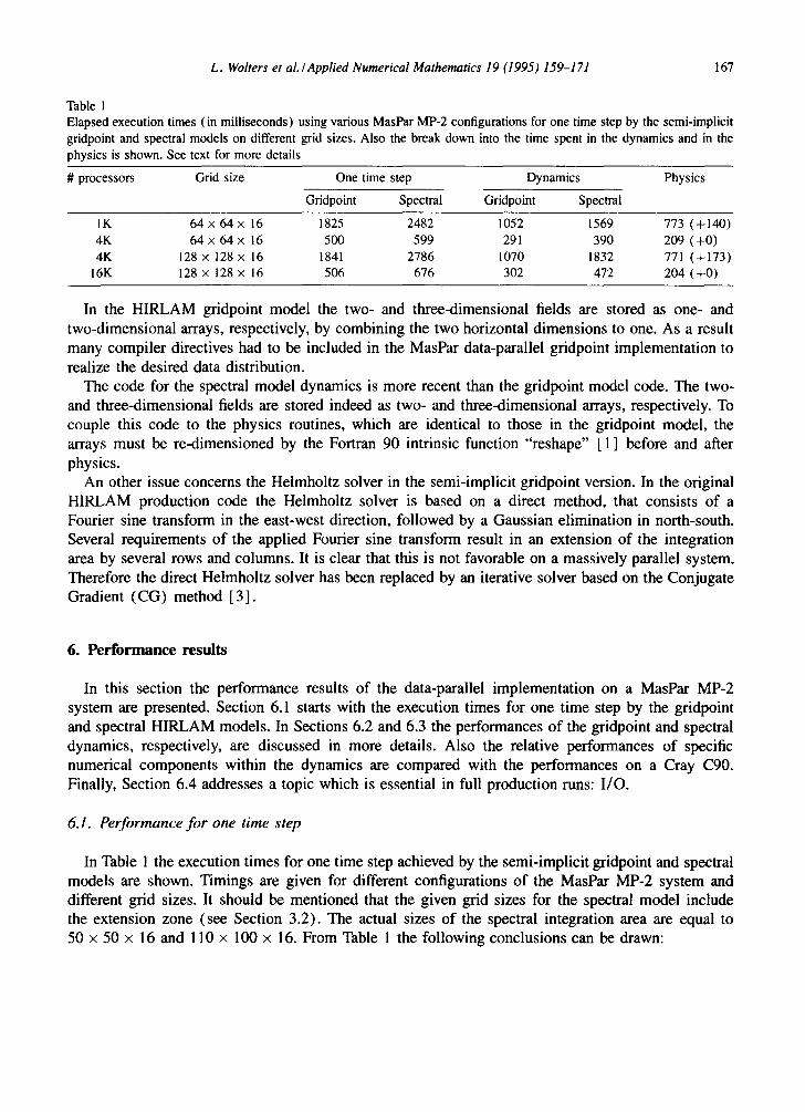
Table 1 Elapsed execution times (in milliseconds) using various MasPar MP-2 configurations for one time step by the semi-implicit gridpoint and spectral models on different grid sizes. Also the break down into the time spent in the dynamics and in the physics is shown. See text for more details

# processors Grid size One time step Dynamics Physics

Gridpoint Spectral Gridpoint Spectral

IK 64 × 64 × 16 1825 2482 1052 1569 773 (+140) 4K 64 x 64 x 16 500 599 291 390 209 (+0) 4K 128 x 128 × 16 1841 2786 1070 1832 771 (+173)

16K 128 × 128 × 16 506 676 302 472 204 (+0)

In the HIRLAM gridpoint model the two- and three-dimensional fields are stored as one- and two-dimensional arrays, respectively, by combining the two horizontal dimensions to one. As a result many compiler directives had to be included in the MasPar data-parallel gridpoint implementation to realize the desired data distribution.

The code for the spectral model dynamics is more recent than the gridpoint model code. The two- and three-dimensional fields are stored indeed as two- and three-dimensional arrays, respectively. To couple this code to the physics routines, which are identical to those in the gridpoint model, the arrays must be re-dimensioned by the Fortran 90 intrinsic function "reshape" [1] before and after physics.

An other issue concerns the Helmholtz solver in the semi-implicit gridpoint version. In the original HIRLAM production code the Helmholtz solver is based on a direct method, that consists of a Fourier sine transform in the east-west direction, followed by a Gaussian elimination in north-south. Several requirements of the applied Fourier sine transform result in an extension of the integration area by several rows and columns. It is clear that this is not favorable on a massively parallel system. Therefore the direct Helmholtz solver has been replaced by an iterative solver based on the Conjugate Gradient (CG) method [ 3 ].

6. Performance results

In this section the performance results of the data-parallel implementation on a MasPar MP-2 system are presented. Section 6.1 starts with the execution times for one time step by the gridpoint and spectral HIRLAM models. In Sections 6.2 and 6.3 the performances of the gridpoint and spectral dynamics, respectively, are discussed in more details. Also the relative performances of specific numerical components within the dynamics are compared with the performances on a Cray C90. Finally, Section 6.4 addresses a topic which is essential in full production runs: I/O.

6.1. Performance for one time step

In Table 1 the execution times for one time step achieved by the semi-implicit gridpoint and spectral models are shown. Timings are given for different configurations of the MasPar MP-2 system and different grid sizes. It should be mentioned that the given grid sizes for the spectral model include the extension zone (see Section 3.2). The actual sizes of the spectral integration area are equal to 50 x 50 × 16 and 110 x 100 × 16. From Table 1 the following conclusions can be drawn:


Table 2 Elapsed execution times (in milliseconds) using various MasPar MP-2 configurations split into the different components of the gridpoint dynamics. See text for details

# processors Grid size Dynamical Horizontal Semi-implicit Others

tendencies diffusion Total CG

IK 64 × 64 x 16 243 118 409 184 282 4K 64 × 64 x 16 44 22 149 84 76 4K 128 x 128 x 16 242 119 430 204 279

16K 128 x 128 x 16 44 22 163 97 73

- The elapsed times for one time step show that the spectral model takes 20-50% more time than the gridpoint model. Limited to the essential difference between the two models, which is the dynamics, one sees a 30-70% increase in execution time.

- Since the physics code is the same for both models, the timings for the physics should be equal. However, the necessary "reshaping" of the data structures in the spectral model (see Section 5) requires extra time, which is given in parentheses in the "physics" column. In case the number of datapoints is larger than the number of processors this time becomes substantial.

In the next sections the achieved times for both models will be investigated in more detail.

6.2. Gridpoint model profile

Table 2 shows an execution profile for the semi-implicit gridpoint dynamics. The different components within one time step were discussed in Sections 3.1 and 3.3. The elapsed time for one time step is divided into the time for calculating the explicit dynamical tendencies, the time to carry out the horizontal diffusion, the total costs for the semi-implicit corrections, and the time for other routines. These routines are e.g. the time filter, time stepping, boundary relaxation, extension of fields. The execution time for the CG algorithm is presented separately. Based on Table 2 the following observations can be made:

- Four times as many processors allows four times more gridpoints. It results in the same elapsed time for each components except for CG. To obtain the same accuracy the number of iterations in CG is increased by approximately 10% for the larger grid compared to the smaller one.

- The calculations of the dynamical tendencies and the horizontal diffusion show a superlinear behavior with respect to an increase in the number of processors. This does not hold for the semi-implicit costs, in particular again for CG.

- The execution time for a fully explicit version can also be derived from this table: the time spent in the semi-implicit part should be subtracted from the total time, but the time step for the dynamics should be five time smaller. It is clear that these two changes do not compensate; the total execution time for a fully explicit version is approximately 2-3 times larger than for the semi-implicit model.

Comparing this implementation with an implementation on a vector architecture shows also some interesting differences. On a one-processor Cray C90 the following numbers can be measured for the HIRLAM reference code: during one time step ( ~ 3.5 s for a 128 x 128 x 16 grid) 40% of the total time is spent in the dynamics, of which 17% in calculating the dynamical tendencies, 5% in the horizontal diffusion, 11% in the semi-implicit calculations, and 7% in other routines. The


physics takes 60%. Before discussing the differences with the MasPar implementation, some remarks concerning the Cray profile should be made: ( 1 ) this relative profile is almost independent of the grid size; (2) it is based on an implementation of the HIRLAM reference code, and therefore contains the original Helmholtz solver (see Section 5); (3) the calculations on the Cray are in 64 bits, while they are in 32 bits on the MasPar. The reason is that we have not seen that 32 bits is insufficient for the HIRLAM model at the resolution studied here. Therefore the best comparison should be between a 32-bits MasPar and 32-bits Cray. However, this last machine is not available, so the Cray is too expensive for its purpose.

Concerning the differences between the MasPar and Cray results the following observations can be made:

- The ratio between execution times for the dynamics and the physics is significantly different; on the MP-2 60% and 40% for the dynamics and the physics, respectively, while for the C90 these numbers are 40% and 60%.

- The time for the semi-implicit corrections is significantly smaller on the C90 compared to the results on the MP-2.

- On the MasPar the "other" routines contribute considerably more to the total elapsed time than on the Cray (15% versus 7%).

6.3. Spectral model profile

Profiling the spectral model on the MP-2 and the C90 results in the following observations: - The most important factor in the total execution time is determined by the FFTs. For a 128 ×

128 x 16 grid the FFTs contribute for 75% to the dynamics on the MP-2. On the C90 this number is 65%.

- The spectral version is not scalable with respect to number of datapoints. This can also be seen from Table 1. The reason for this fact are the b-TTs.

- The ratio's between the execution times of the dynamics and of the physics on the MP-2 and C90 are again significantly different: on the MP-2 65-70% for the dynamics and 30-35% for the physics, and on the C90 one observes 45% for the dynamics and 55% for the physics.

6.4. Full production runs

Full production runs of a numerical forecast model contain two aspects that have not been addressed yet: I /O and pre/post-processing. Examples of input are the initial and lateral boundary data. The output consists for instance of the calculated fields. All these data are given as binary packed records, with the number of bits for each value in a particular field determined from the required accuracy and the actual range of variation for that particular field. This GRIB (gridded binary) format is a standard for storage and exchange of processed data within the meteorological community. The pre/post-processing routines transform these GRIB files into internal computer words and vice versa.

We have demonstrated [ 17,18] that I /O and pre/post-processing should be considered as important issues on a massively parallel system like MasPar. The time spent in these parts of a full production run could easily double the total execution time. This was mainly due to the fact that these routines were not parallelized and therefore were executed on the front-end.

170 L. Wohers et al./ Applied Numerical Mathematics 19 (1995) 159-171

Table 3 Profiling of pre/post-processing versus model integration

Stage in forecast MasPar MP-2, 16K Convex C-3840, 4 proc.

Input, unpacking, and pre-processing 8.7% 3.7% Time integration 83.1% 92.9% Post-processing, packing, and output 8.2% 3.4%

Table 3 shows some results if one makes the effort to parallelize the routines involved with I /O and pre/post-processing. A comparison with a four-processor Convex C-3840 is also presented. From this table is can be concluded that contrary to what previously pessimistically has been estimated [ 17] the MasPar MP-2 shows to be capable of handling the I /O needed for a full operational forecast run. Compared to the results on the Convex the MP-2 percentages are still high.

It should be noticed that these percentages are strongly dependent on the amount of data, in which the modeller is interested. This can be specified by the user. In particular the frequency by which calculated field should be stored on disk, will influence the total post-processing and I /O time significantly with respect to the model integration time. Therefore the role of these issues on the performance of full production runs on parallel systems should not be underestimated.

7. Concluding remarks

This investigation has resulted in a detailed performance comparison of different numerical methods applied in the operational HIRLAM weather forecast model. The conclusions are listed and discussed in Section 6. The fact that nonnumerical aspects within such a model are also important, has been demonstrated in Section 6.4.

It is not clear yet, whether massively parallel computer systems will be applied for numerical weather forecasting in the near future. It requires more research, in particular other parallel architectures should be investigated. Furthermore, not only the forecast model should run efficiently, but also the other important part of a forecast system, namely the analysis part dealing with the observations, has to be implemented on such an architecture. However, the experiments in this investigation demonstrate at least that a MasPar massively parallel system can provide an interesting alternative to vector architectures, since scalability of the numerical algorithms in the HIRLAM forecast model varies from reasonable to very good.

References

[ 1 ] J.C. Adams, W.S. Brainerd, S. Walter and J.T. Martin, Fortran 90 Handbook (Intertext, New York, 1992). [2] A. Arakawa and V.R. Lamb, Computational design of the basic dynamical processes of the ULCA general circulation

model, Report, Department of Meteorology, University of California, Los Angeles, CA (1976). [3] J.W. Demmel, M.T. Heath and H.A. van der Vorst, Parallel numerical linear algebra, Acta Numerica 2 (1993) I 11-197. [4] E. Eliassen, B. Machenhauer and E. Rasmussen, On a numerical method for integration of the hydrodynamical

equations with a spectral representation of the horizontal fields, Report No. 2, Institute for Theoretical Meteorology, University of Copenhagen, Copenhagen (1970).

[5 ] N. Gustafsson, The HIRLAM model, in: Proceedings Seminar on Numerical Methods in Atmospheric Models, Reading ( 1991 ).

L. Wolters et al. / Applied Numerical Mathematics 19 (1995) 159-171 171

[6] N. Gustafsson, ed., The HIRLAM 2 Final Report, HIRLAM Tech. Rept. 9 (1993) (available from SMHI, S-60176 NorrkOping, Sweden).

[7] G.J. Haltiner and R.T. Williams, Numerical Prediction and Dynamic Meteorology (Wiley, New York, 2nd ed., 1980). [ 8 ] J.E. Haugen and B. Machenhauer, A spectral limited-area model formulation with time-dependent boundary conditions

applied to the shallow-water equations, Mon. Wea. Rev. 121 (1993) 2631-2636. [9] P. K~tliberg and R. Gibson, Lateral boundary conditions for a limited area version of the ECMWF model, WGNE

Progress Report No. 14., WMO, Geneva (1977). [ 10] P. Kftllberg, ed., Documentation Manual of the Hirlam Level 1 Analysis-Forecast System (1990). [ 11 ] B. Machenhauer, The spectral method, in: Numerical Methods used in Atmospheric Models Vol. II, GARP Publication

Series 17 (1979) 124-277. [ 12] B. Machenhauer, ed., The HIRLAM Final Report, HIRLAM Tech. Rept. 5, DMI, Copenhagen (1988). [ 13] MasPar, MasPar MP-I Hardware Manuals (1992). [ 14] H. Munthe-Kaas, Super parallel FFFs, SlAM J. Sci. Statist. Comput. 14 (1993) 349-367. [ 15] S.A. Orzag, Transform method for calculation of vector-coupled sums; application to the spectral form of the vorticity

equation, J. Atmospheric Sci. 27 (1970) 890-895. [ 16] A.J. Simmons, Some aspects of the design and performance of the global ECMWF spectral model, in: Proceedings

Workshop on Techniques for Horizontal Discretization in Numerical Weather Prediction Models, ECMWF, Reading (1987) 249-304.

[ 17] L. Wolters, G. Cats and N. Gustafsson, Limited area numerical weather forecasting on a massively parallel computer, in: Proceedings 8th ACM International Conference on Supercomputing, Manchester (ACM, New York, 1994) 289-296.

[ 18] L. Wolters, G. Cats and N. Gustafsson, Data-parallel numerical weather forecasting, Sci. Programming 4 (1995) 141-153.

Documents

Data-parallel numerical methods in a weather forecast model